Embed Size (px)
Citation preview
This is page iPrinter: Opaque this
Contents
A Linear algebra basics 1A.1 Basic operations . . . . . . . . . . . . . . . . . . . . . . . . 1A.2 Fundamental theorem of linear algebra . . . . . . . . . . . . 4
A.2.1 Part one . . . . . . . . . . . . . . . . . . . . . . . . . 4A.2.2 Part two . . . . . . . . . . . . . . . . . . . . . . . . . 5
A.3 Nature of the solution . . . . . . . . . . . . . . . . . . . . . 7A.3.1 Exactly-identified . . . . . . . . . . . . . . . . . . . . 7A.3.2 Under-identified . . . . . . . . . . . . . . . . . . . . 8A.3.3 Over-identified . . . . . . . . . . . . . . . . . . . . . 11
A.4 Matrix decomposition and inverse operations . . . . . . . . 13A.4.1 LU factorization . . . . . . . . . . . . . . . . . . . . 13A.4.2 Cholesky decomposition . . . . . . . . . . . . . . . . 17A.4.3 Eigenvalues and eigenvectors . . . . . . . . . . . . . 18A.4.4 Singular value decomposition . . . . . . . . . . . . . 24A.4.5 Spectral decomposition . . . . . . . . . . . . . . . . 29A.4.6 quadratic forms, eigenvalues, and positive definiteness 30A.4.7 similar matrices, Jordan form, and generalized eigen-
vectors . . . . . . . . . . . . . . . . . . . . . . . . . . 30A.5 Gram-Schmidt construction of an orthogonal matrix . . . . 33
A.5.1 QR decomposition . . . . . . . . . . . . . . . . . . . 35A.5.2 Gram-Schmidt QR algorithm . . . . . . . . . . . . . 35A.5.3 Accounting example . . . . . . . . . . . . . . . . . . 36A.5.4 The Householder QR algorithm . . . . . . . . . . . . 37A.5.5 Accounting example . . . . . . . . . . . . . . . . . . 37
ii Contents
A.6 Computing eigenvalues . . . . . . . . . . . . . . . . . . . . . 40A.6.1 Schur’s lemma . . . . . . . . . . . . . . . . . . . . . 40A.6.2 Power algorithm . . . . . . . . . . . . . . . . . . . . 41A.6.3 QR algorithm . . . . . . . . . . . . . . . . . . . . . . 42A.6.4 Schur decomposition . . . . . . . . . . . . . . . . . . 44
A.7 Some determinant identities . . . . . . . . . . . . . . . . . . 47A.7.1 Determinant of a square matrix . . . . . . . . . . . . 47A.7.2 Identities . . . . . . . . . . . . . . . . . . . . . . . . 48
A.8 Matrix exponentials and logarithms . . . . . . . . . . . . . 50
B Iterated expectations 53B.1 Decomposition of variance . . . . . . . . . . . . . . . . . . . 55B.2 Jensen’s inequality . . . . . . . . . . . . . . . . . . . . . . . 56
C Multivariate normal theory 57C.1 Conditional distribution . . . . . . . . . . . . . . . . . . . . 59C.2 Special case of precision . . . . . . . . . . . . . . . . . . . . 63C.3 Truncated normal distribution . . . . . . . . . . . . . . . . 65
D Projections and conditional expectations 73D.1 Gauss-Markov theorem . . . . . . . . . . . . . . . . . . . . . 73D.2 Generalized least squares (GLS) . . . . . . . . . . . . . . . . 76D.3 Recursive least squares . . . . . . . . . . . . . . . . . . . . . 78
E Two stage least squares IV (2SLS-IV) 81E.1 General case . . . . . . . . . . . . . . . . . . . . . . . . . . . 81E.2 Special case . . . . . . . . . . . . . . . . . . . . . . . . . . . 83
F Seemingly unrelated regression (SUR) 85F.1 Classical . . . . . . . . . . . . . . . . . . . . . . . . . . . . . 86F.2 Bayesian . . . . . . . . . . . . . . . . . . . . . . . . . . . . . 86F.3 Bayesian treatment effect application . . . . . . . . . . . . . 87
G Maximum likelihood estimation of discrete choice models 89
H Optimization 91H.1 Linear programming . . . . . . . . . . . . . . . . . . . . . . 91
H.1.1 basic solutions or extreme points . . . . . . . . . . . 92H.1.2 fundamental theorem of linear programming . . . . . 93H.1.3 duality theorems . . . . . . . . . . . . . . . . . . . . 93H.1.4 example . . . . . . . . . . . . . . . . . . . . . . . . . 94H.1.5 complementary slackness . . . . . . . . . . . . . . . 94
H.2 Nonlinear programming . . . . . . . . . . . . . . . . . . . . 95H.2.1 unconstrained . . . . . . . . . . . . . . . . . . . . . . 95H.2.2 convexity and global minima . . . . . . . . . . . . . 95H.2.3 example . . . . . . . . . . . . . . . . . . . . . . . . . 96
Contents iii
H.2.4 constrained – the Lagrangian . . . . . . . . . . . . 96H.2.5 Karash-Kuhn-Tucker conditions . . . . . . . . . . . . 97H.2.6 example . . . . . . . . . . . . . . . . . . . . . . . . . 98
H.3 Theorem of the separating hyperplane . . . . . . . . . . . . 99
I Quantum information 101I.1 Quantum information axioms . . . . . . . . . . . . . . . . . 101
I.1.1 The superposition axiom . . . . . . . . . . . . . . . . 101I.1.2 The transformation axiom . . . . . . . . . . . . . . . 102I.1.3 The measurement axiom . . . . . . . . . . . . . . . . 102I.1.4 The combination axiom . . . . . . . . . . . . . . . . 103
I.2 Summary of quantum "rules" . . . . . . . . . . . . . . . . . 105I.3 Observables and expected payoffs . . . . . . . . . . . . . . . 106I.4 Density operators and quantum entropy . . . . . . . . . . . 107
I.4.1 Quantum entropy . . . . . . . . . . . . . . . . . . . 110I.5 Some trigonometric identities . . . . . . . . . . . . . . . . . 110
J Common distributions 113

iv Contents
This is page 1Printer: Opaque this
Appendix ALinear algebra basics
A.1 Basic operations
We frequently envision or frame problems as linear systems of equations.1
It is useful to write this compactly in matrix notation, say
Ay = x
where A is an m × n (rows × columns) matrix (a rectangular array ofelements), y is an n-element vector, and x is an m-element vector. Thisstatement compares the result on the left with that on the right, element-by-element. The operation on the left is matrix multiplication or each ele-ment is recovered by a vector inner product of the corresponding row fromA with the vector y. That is, the first element of the product vector Ay isthe vector inner product of the first row A with y, the second element ofthe product vector is the inner product of the second row A with y, andso on. A vector inner product multiplies the same position element of theleading row and trailing column and sums over the products. Of course, thismeans that the operation is only well-defined if the number of columns inthe leading matrix, A, equals the number of rows of the trailing, y. Further,the product matrix has the same number of rows as the leading matrix and
1G. Strang, Linear Algebra and its Applications, Harcourt Brace Jovanovich Col-lege Publishers, or Introduction to Linear Algebra, Wellesley-Cambridge Press offers amesmerizing discourse on linear algebra.
2 Appendix A. Linear algebra basics
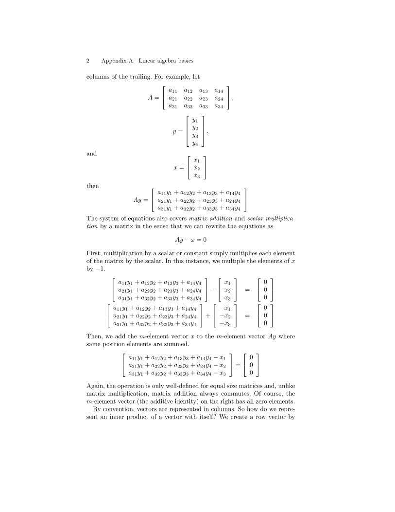
columns of the trailing. For example, let
A =
a11 a12 a13 a14
a21 a22 a23 a24
a31 a32 a33 a34
,
y =
y1
y2
y3
y4
,and
x =
x1
x2
x3
then
Ay =
a11y1 + a12y2 + a13y3 + a14y4
a21y1 + a22y2 + a23y3 + a24y4
a31y1 + a32y2 + a33y3 + a34y4
The system of equations also covers matrix addition and scalar multiplica-tion by a matrix in the sense that we can rewrite the equations as
Ay − x = 0
First, multiplication by a scalar or constant simply multiplies each elementof the matrix by the scalar. In this instance, we multiple the elements of xby −1. a11y1 + a12y2 + a13y3 + a14y4
a21y1 + a22y2 + a23y3 + a24y4
a31y1 + a32y2 + a33y3 + a34y4
− x1
x2
x3
=
000
a11y1 + a12y2 + a13y3 + a14y4
a21y1 + a22y2 + a23y3 + a24y4
a31y1 + a32y2 + a33y3 + a34y4
+
−x1
−x2
−x3
=
000
Then, we add the m-element vector x to the m-element vector Ay wheresame position elements are summed. a11y1 + a12y2 + a13y3 + a14y4 − x1
a21y1 + a22y2 + a23y3 + a24y4 − x2
a31y1 + a32y2 + a33y3 + a34y4 − x3
=
000
Again, the operation is only well-defined for equal size matrices and, unlikematrix multiplication, matrix addition always commutes. Of course, them-element vector (the additive identity) on the right has all zero elements.By convention, vectors are represented in columns. So how do we repre-
sent an inner product of a vector with itself? We create a row vector by
A.1 Basic operations 3
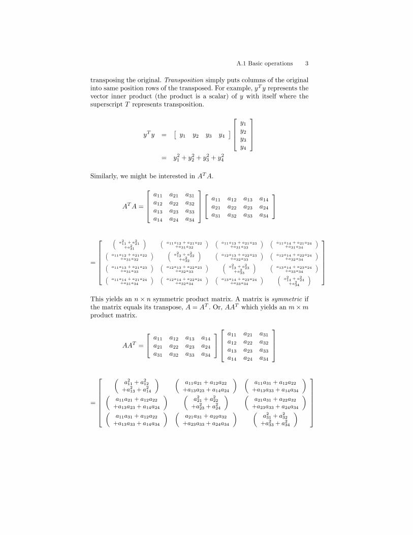
transposing the original. Transposition simply puts columns of the originalinto same position rows of the transposed. For example, yT y represents thevector inner product (the product is a scalar) of y with itself where thesuperscript T represents transposition.
yT y =[y1 y2 y3 y4
] y1
y2
y3
y4
= y2
1 + y22 + y2
3 + y24
Similarly, we might be interested in ATA.
ATA =
a11 a21 a31
a12 a22 a32
a13 a23 a33
a14 a24 a34
a11 a12 a13 a14
a21 a22 a23 a24
a31 a32 a33 a34
=
(a211 + a221+a231
) (a11a12 + a21a22
+a31a32
) (a11a13 + a21a23
+a31a33
) (a11a14 + a21a24
+a31a34
)(a11a12 + a21a22
+a31a32
) (a212 + a222+a232
) (a12a13 + a22a23
+a32a33
) (a12a14 + a22a24
+a32a34
)(a11a13 + a21a23
+a31a33
) (a12a13 + a22a23
+a32a33
) (a213 + a223+a233
) (a13a14 + a23a24
+a33a34
)(a11a14 + a21a24
+a31a34
) (a12a14 + a22a24
+a32a34
) (a13a14 + a23a24
+a33a34
) (a214 + a224+a234
)
This yields an n× n symmetric product matrix. A matrix is symmetric ifthe matrix equals its transpose, A = AT . Or, AAT which yields an m×mproduct matrix.
AAT =
a11 a12 a13 a14
a21 a22 a23 a24
a31 a32 a33 a34
a11 a21 a31
a12 a22 a32
a13 a23 a33
a14 a24 a34
=
(a211 + a
212
+a213 + a214
) (a11a21 + a12a22+a13a23 + a14a24
) (a11a31 + a12a22+a13a33 + a14a34
)(
a11a21 + a12a22+a13a23 + a14a24
) (a221 + a
222
+a223 + a224
) (a21a31 + a22a32+a23a33 + a24a34
)(
a11a31 + a12a22+a13a33 + a14a34
) (a21a31 + a22a32+a23a33 + a24a34
) (a231 + a
232
+a233 + a234
)
4 Appendix A. Linear algebra basics
A.2 Fundamental theorem of linear algebra
With these basic operations in hand, return to
Ay = x
When is there a unique solution, y? The answer lies in the fundamentaltheorem of linear algebra. The theorem has two parts.
A.2.1 Part one
First, the theorem says that for every matrix the number of linearly inde-pendent rows equals the number of linearly independent columns. Linearlyindependent vectors are the set of vectors such that no one of them can beduplicated by a linear combination of the other vectors in the set. A lin-ear combination of vectors is the sum of scalar-vector products where eachvector may have a different scalar multiplier. For example, Ay is a linearcombination of the columns of A with the scalars in y. Therefore, if there ex-ists some (n− 1)-element vector, w, when multiplied by an (m× (n− 1))submatrix of A, call it B, such that Bw produces the dropped columnfrom A then the dropped column is not linearly independent of the othercolumns. To reiterate, if the matrix A has r linearly independent columns italso has r linearly independent rows. r is referred to as the rank of the ma-trix and dimension of the rowspace and columnspace (the spaces spannedby all possible linear combination of the rows and columns, respectively).Further, r linearly independent rows of A form a basis for its rowspace andr linearly independent columns of A form a basis for its columnspace.
Accounting example
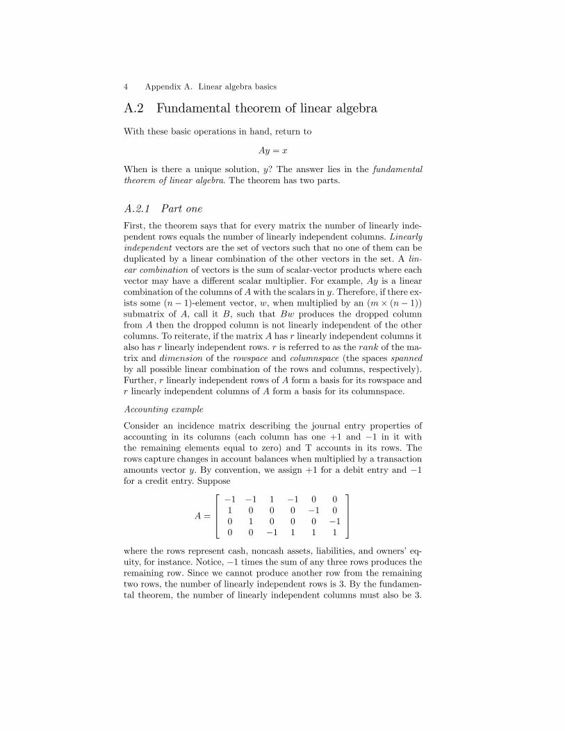
Consider an incidence matrix describing the journal entry properties ofaccounting in its columns (each column has one +1 and −1 in it withthe remaining elements equal to zero) and T accounts in its rows. Therows capture changes in account balances when multiplied by a transactionamounts vector y. By convention, we assign +1 for a debit entry and −1for a credit entry. Suppose
A =
−1 −1 1 −1 0 01 0 0 0 −1 00 1 0 0 0 −10 0 −1 1 1 1
where the rows represent cash, noncash assets, liabilities, and owners’eq-uity, for instance. Notice, −1 times the sum of any three rows produces theremaining row. Since we cannot produce another row from the remainingtwo rows, the number of linearly independent rows is 3. By the fundamen-tal theorem, the number of linearly independent columns must also be 3.
A.2 Fundamental theorem of linear algebra 5
Let’s check. Suppose the first three columns is a basis for the columnspace.Column 4 is the negative of column 3, column 5 is the negative of the sumof columns 1 and 3, and column 6 is the negative of the sum of columns 2and 3. Can any of columns 1, 2 and 3 be produced as a linearly combinationof the remaining two columns? No, the zeroes in rows 2 through 4 rule itout. For this matrix, we’ve confirmed the number of linearly independentrows and columns is the same.
A.2.2 Part two
The second part of the fundamental theorem describes the orthogonal com-plements to the rowspace and columnspace. Two vectors are orthogonal ifthey are perpendicular to one another. As their vector inner product isproportional to the cosine of the angle between them, if their vector innerproduct is zero they are orthogonal.2 n-space is spanned by the rowspace(with dimension r) plus the n − r dimension orthogonal complement, thenullspace where
ANT = 0
N is an (n− r)×n matrix whose rows are orthogonal to the rows of A and0 is an m× (n− r) matrix of zeroes.
Accounting example continued
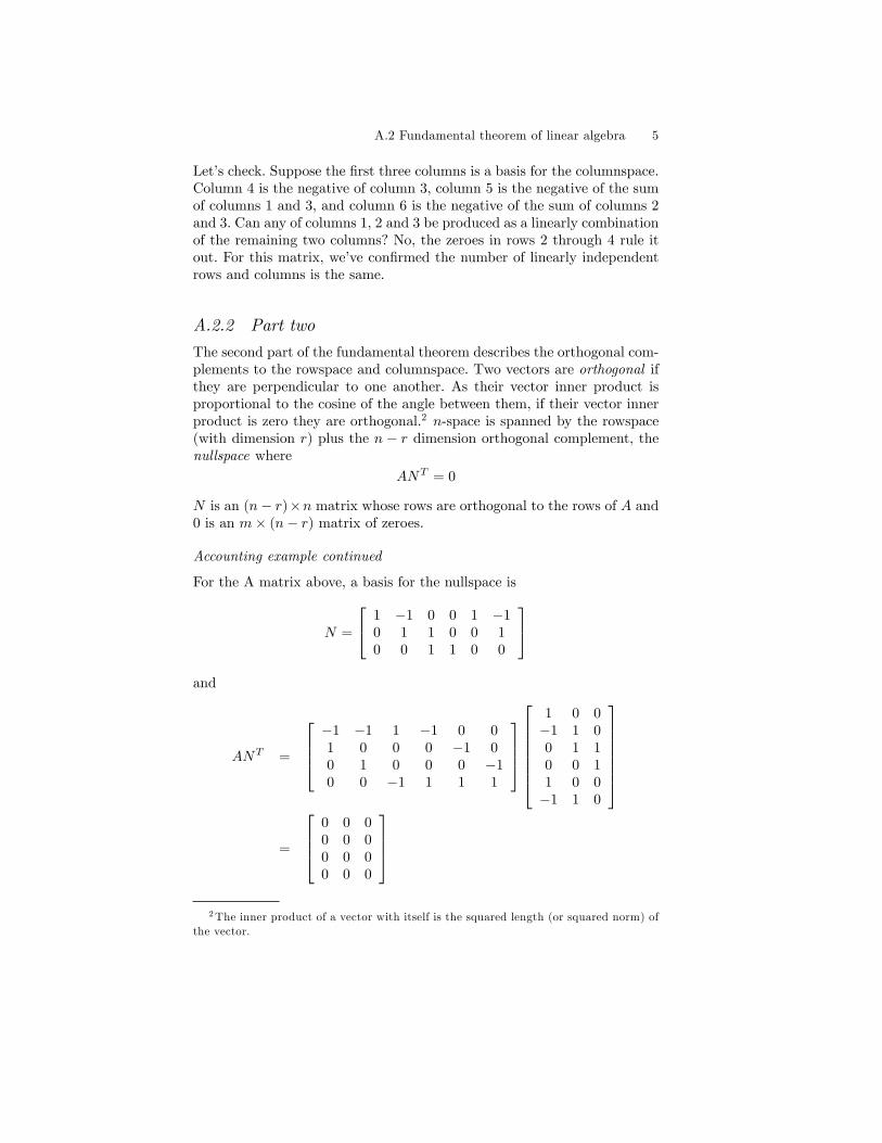
For the A matrix above, a basis for the nullspace is
N =
1 −1 0 0 1 −10 1 1 0 0 10 0 1 1 0 0
and
ANT =
−1 −1 1 −1 0 01 0 0 0 −1 00 1 0 0 0 −10 0 −1 1 1 1
1 0 0−1 1 00 1 10 0 11 0 0−1 1 0
=
0 0 00 0 00 0 00 0 0
2The inner product of a vector with itself is the squared length (or squared norm) of
the vector.
6 Appendix A. Linear algebra basics
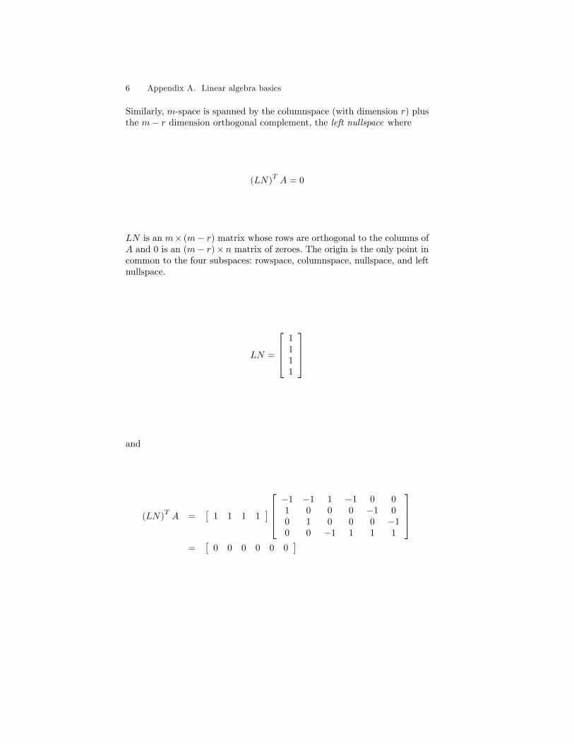
Similarly, m-space is spanned by the columnspace (with dimension r) plusthe m− r dimension orthogonal complement, the left nullspace where
(LN)TA = 0
LN is an m× (m− r) matrix whose rows are orthogonal to the columns ofA and 0 is an (m− r)× n matrix of zeroes. The origin is the only point incommon to the four subspaces: rowspace, columnspace, nullspace, and leftnullspace.
LN =
1111
and
(LN)TA =
[1 1 1 1
] −1 −1 1 −1 0 01 0 0 0 −1 00 1 0 0 0 −10 0 −1 1 1 1
=
[0 0 0 0 0 0
]
A.3 Nature of the solution 7
A.3 Nature of the solution
A.3.1 Exactly-identified
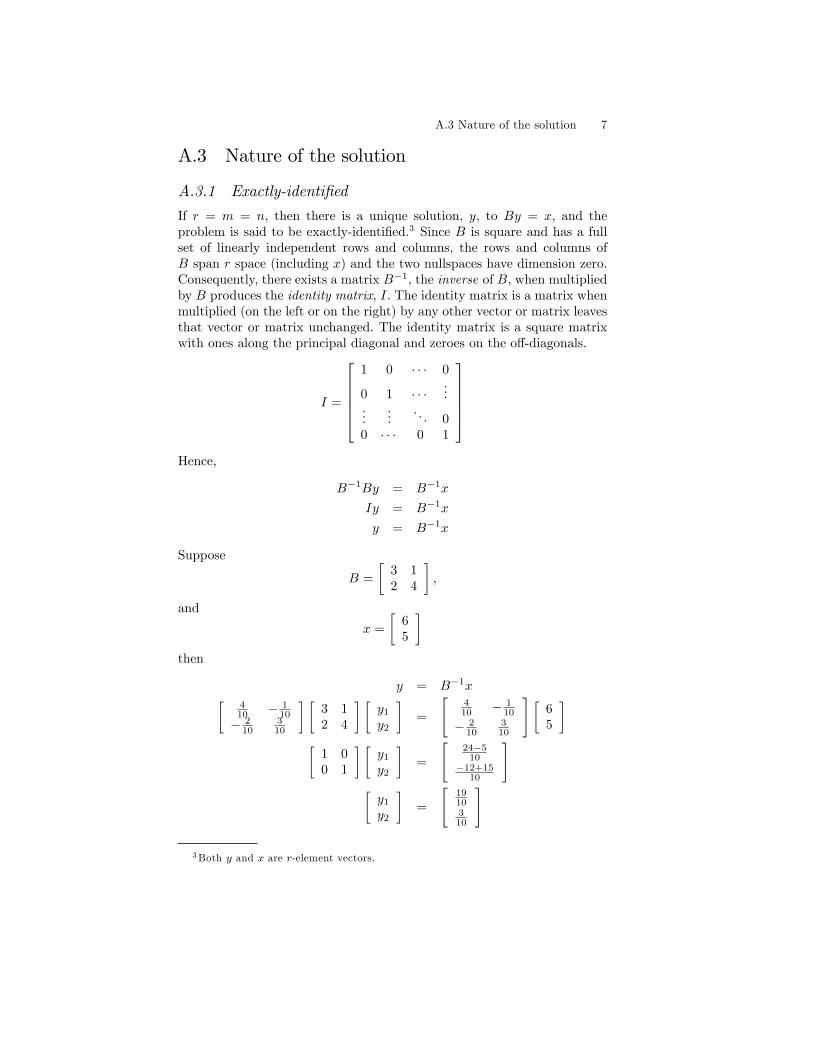
If r = m = n, then there is a unique solution, y, to By = x, and theproblem is said to be exactly-identified.3 Since B is square and has a fullset of linearly independent rows and columns, the rows and columns ofB span r space (including x) and the two nullspaces have dimension zero.Consequently, there exists a matrix B−1, the inverse of B, when multipliedby B produces the identity matrix, I. The identity matrix is a matrix whenmultiplied (on the left or on the right) by any other vector or matrix leavesthat vector or matrix unchanged. The identity matrix is a square matrixwith ones along the principal diagonal and zeroes on the off-diagonals.
I =
1 0 · · · 0
0 1 · · ·...
......
. . . 00 · · · 0 1
Hence,
B−1By = B−1x
Iy = B−1x
y = B−1x
Suppose
B =
[3 12 4
],
and
x =
[65
]then
y = B−1x[410 − 1
10− 2
10310
] [3 12 4
] [y1
y2
]=
[410 − 1
10
− 210
310
] [65
][
1 00 1
] [y1
y2
]=
[24−5
10−12+15
10
][y1
y2
]=
[1910310
]
3Both y and x are r-element vectors.
8 Appendix A. Linear algebra basics
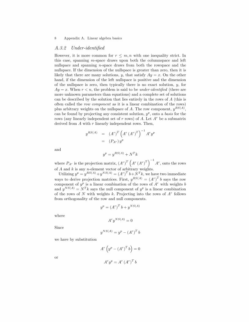
A.3.2 Under-identified
However, it is more common for r ≤ m,n with one inequality strict. Inthis case, spanning m-space draws upon both the columnspace and leftnullspace and spanning n-space draws from both the rowspace and thenullspace. If the dimension of the nullspace is greater than zero, then it islikely that there are many solutions, y, that satisfy Ay = x. On the otherhand, if the dimension of the left nullspace is positive and the dimensionof the nullspace is zero, then typically there is no exact solution, y, forAy = x. When r < n, the problem is said to be under-identified (there aremore unknown parameters than equations) and a complete set of solutionscan be described by the solution that lies entirely in the rows of A (this isoften called the row component as it is a linear combination of the rows)plus arbitrary weights on the nullspace of A. The row component, yRS(A),can be found by projecting any consistent solution, yp, onto a basis for therows (any linearly independent set of r rows) of A. Let Ar be a submatrixderived from A with r linearly independent rows. Then,
yRS(A) = (Ar)T(Ar (Ar)
T)−1
Aryp
= (PAr ) yp
andyp = yRS(A) +NT k
where PAr is the projection matrix, (Ar)T(Ar (Ar)
T)−1
Ar, onto the rows
of A and k is any n-element vector of arbitrary weights.Utilizing yp = yRS(A) +yNS(A) = (Ar)
Tb+NT k, we have two immediate
ways to derive projection matrices. First, yRS(A) = (Ar)Tb says the row
component of yp is a linear combination of the rows of Ar with weights band yNS(A) = NT k says the null component of yp is a linear combinationof the rows of N with weights k. Projecting into the rows of Ar followsfrom orthogonality of the row and null components.
yp = (Ar)Tb+ yNS(A)
whereAryNS(A) = 0
SinceyNS(A) = yp − (Ar)
Tb
we have by substitution
Ar(yp − (Ar)
Tb)
= 0
orAryp = Ar (Ar)
Tb
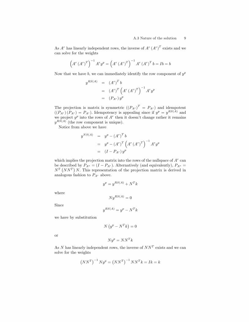
A.3 Nature of the solution 9
As Ar has linearly independent rows, the inverse of Ar (Ar)T exists and we
can solve for the weights(Ar (Ar)
T)−1
Aryp =(Ar (Ar)
T)−1
Ar (Ar)Tb = Ib = b
Now that we have b, we can immediately identify the row component of yp
yRS(A) = (Ar)Tb
= (Ar)T(Ar (Ar)
T)−1
Aryp
= (PAr ) yp
The projection is matrix is symmetric ((PAr )T
= PAr ) and idempotent((PAr ) (PAr ) = PAr ). Idempotency is appealing since if yp = yRS(A) andwe project yp into the rows of Ar then it doesn’t change rather it remainsyRS(A) (the row component is unique).Notice from above we have
yNS(A) = yp − (Ar)Tb
= yp − (Ar)T(Ar (Ar)
T)−1
Aryp
= (I − PAr ) yp
which implies the projection matrix into the rows of the nullspace of Ar canbe described by PAn = (I − PAr ). Alternatively (and equivalently), PAn =NT
(NNT
)N . This representation of the projection matrix is derived in
analogous fashion to PAr above.
yp = yRS(A) +NT k
whereNyRS(A) = 0
SinceyRS(A) = yp −NT k
we have by substitution
N(yp −NT k
)= 0
orNyp = NNT k
As N has linearly independent rows, the inverse of NNT exists and we cansolve for the weights(
NNT)−1
Nyp =(NNT
)−1NNT k = Ik = k
10 Appendix A. Linear algebra basics
Now that we have k, we can immediately identify the null component of yp
yNS(A) = NT k
= NT(NNT
)−1Nyp
= (PAn) yp
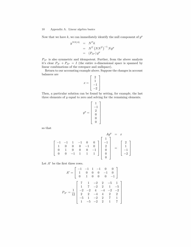
PAn is also symmetric and idempotent. Further, from the above analysisit’s clear PAr + PAn = I (the entire n-dimensional space is spanned bylinear combinations of the rowspace and nullspace).Return to our accounting example above. Suppose the changes in account
balances are
x =
21−1−2
Then, a particular solution can be found by setting, for example, the lastthree elements of y equal to zero and solving for the remaining elements.
yp =
1−12000
so that
Ayp = x−1 −1 1 −1 0 01 0 0 0 −1 00 1 0 0 0 −10 0 −1 1 1 1
1−12000
=
21−1−2
Let Ar be the first three rows.
Ar =
−1 −1 1 −1 0 01 0 0 0 −1 00 1 0 0 0 −1
PAr =1
12
7 1 −2 2 −5 11 7 −2 2 1 −5−2 −2 4 −4 −2 −22 2 −4 4 2 2−5 1 −2 2 7 11 −5 −2 2 1 7
A.3 Nature of the solution 11
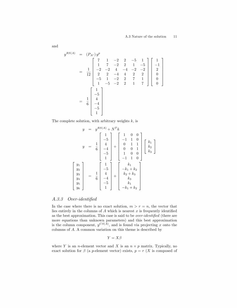
and
yRS(A) = (PAr ) yp
=1
12
7 1 −2 2 −5 11 7 −2 2 1 −5−2 −2 4 −4 −2 −22 2 −4 4 2 2−5 1 −2 2 7 11 −5 −2 2 1 7
1−12000
=1
6
1−54−4−51
The complete solution, with arbitrary weights k, is
y = yRS(A) +NT k
y =1
6
1−54−4−51
+
1 0 0−1 1 00 1 10 0 11 0 0−1 1 0
k1
k2
k3
y1
y2
y3
y4
y5
y6
=1
6
1−54−4−51
+
k1
−k1 + k2
k2 + k3
k3
k1
−k1 + k2
A.3.3 Over-identified
In the case where there is no exact solution, m > r = n, the vector thatlies entirely in the columns of A which is nearest x is frequently identifiedas the best approximation. This case is said to be over-identified (there aremore equations than unknown parameters) and this best approximationis the column component, yCS(A), and is found via projecting x onto thecolumns of A. A common variation on this theme is described by
Y = Xβ
where Y is an n-element vector and X is an n × p matrix. Typically, noexact solution for β (a p-element vector) exists, p = r (X is composed of
12 Appendix A. Linear algebra basics
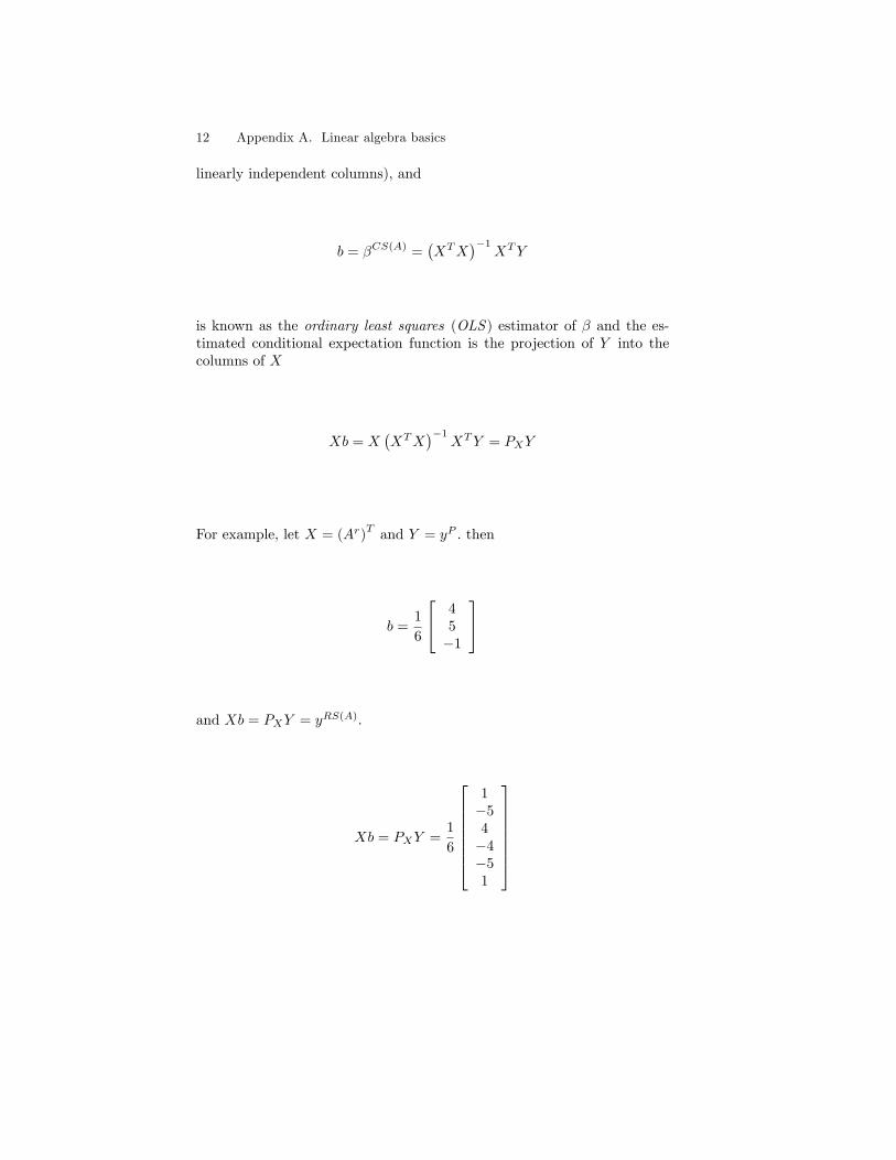
linearly independent columns), and
b = βCS(A) =(XTX
)−1XTY
is known as the ordinary least squares (OLS ) estimator of β and the es-timated conditional expectation function is the projection of Y into thecolumns of X
Xb = X(XTX
)−1XTY = PXY
For example, let X = (Ar)T and Y = yP . then
b =1
6
45−1
and Xb = PXY = yRS(A).
Xb = PXY =1
6
1−54−4−51
A.4 Matrix decomposition and inverse operations 13
A.4 Matrix decomposition and inverse operations
Inverse operations are inherently related to the fundamental theorem andmatrix decomposition. There are a number of important decompositions,we’ll focus on four: LU factorization, Cholesky decomposition, singularvalue decomposition, and spectral decomposition.
A.4.1 LU factorization
Gaussian elimination is the key to solving systems of linear equations andgives us LU decomposition.
Nonsingular case
Any square, nonsingular matrix A (has linearly independent rows andcolumns) can be written as the product of a lower triangular matrix, L,times an upper triangular matrix, U .4
A = LU
where L is lower triangular meaning that it has all zero elements abovethe main diagonal and U is upper triangular meaning that it has all zeroelements below the main diagonal. Gaussian elimination says we can writeany system of linear equations in triangular form so that by backwardrecursion we solve a series of one equation, one variable problems. This isaccomplished by row operations: row eliminations and row exchanges. Roweliminations involve a series of operations where a scalar multiple of onerow is added to a target row so that a revised target row is produced untila triangular matrix, L or U , is generated. As the same operation is appliedto both sides (the same row(s) of A and x) equality is maintained. Rowexchanges simply revise the order of both sides (rows of A and elementsof x) to preserve the equality. Of course, the order in which equations arewritten is flexible.In principle then, Gaussian elimination on
Ay = x
involves, for instance, multiplication of both sides by the inverse of L,provided the inverse exists (m = r),
L−1Ay = L−1x
L−1LUy = L−1x
Uy = L−1x
4The general case, A is a m× n matrix, is discussed below.
14 Appendix A. Linear algebra basics
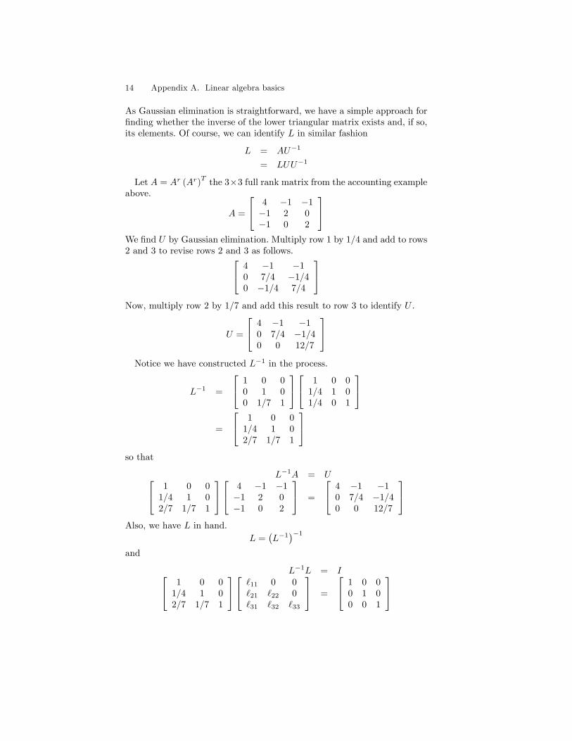
As Gaussian elimination is straightforward, we have a simple approach forfinding whether the inverse of the lower triangular matrix exists and, if so,its elements. Of course, we can identify L in similar fashion
L = AU−1
= LUU−1
Let A = Ar (Ar)T the 3×3 full rank matrix from the accounting example
above.
A =
4 −1 −1−1 2 0−1 0 2
We find U by Gaussian elimination. Multiply row 1 by 1/4 and add to rows2 and 3 to revise rows 2 and 3 as follows. 4 −1 −1
0 7/4 −1/40 −1/4 7/4
Now, multiply row 2 by 1/7 and add this result to row 3 to identify U .
U =
4 −1 −10 7/4 −1/40 0 12/7
Notice we have constructed L−1 in the process.
L−1 =
1 0 00 1 00 1/7 1
1 0 01/4 1 01/4 0 1
=
1 0 01/4 1 02/7 1/7 1
so that
L−1A = U 1 0 01/4 1 02/7 1/7 1
4 −1 −1−1 2 0−1 0 2
=
4 −1 −10 7/4 −1/40 0 12/7
Also, we have L in hand.
L =(L−1
)−1
and
L−1L = I 1 0 01/4 1 02/7 1/7 1
`11 0 0`21 `22 0`31 `32 `33
=
1 0 00 1 00 0 1
A.4 Matrix decomposition and inverse operations 15
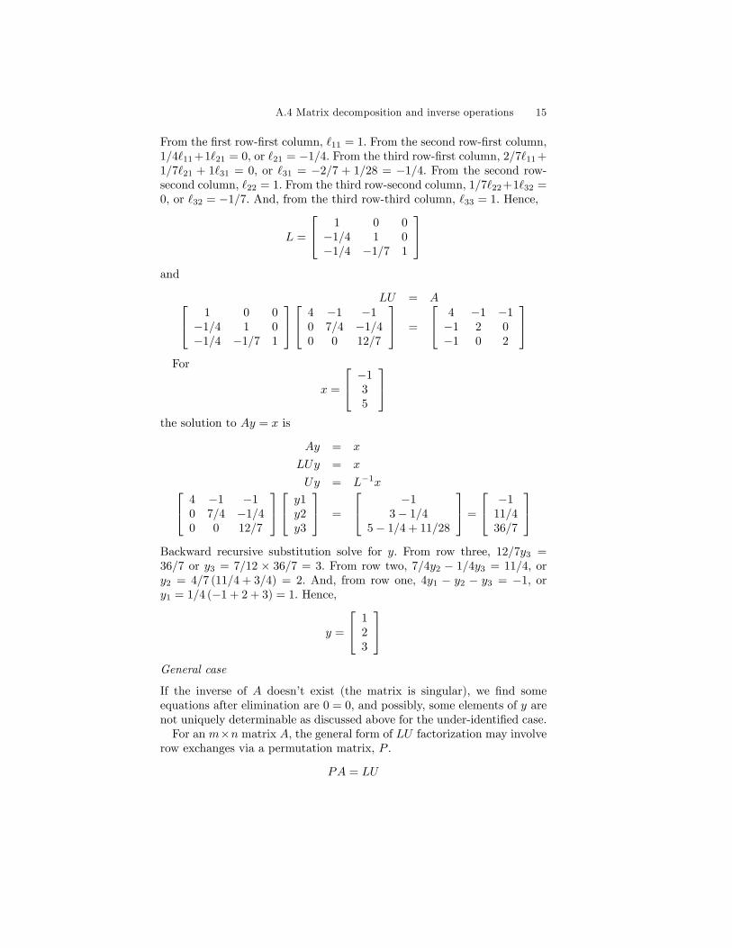
From the first row-first column, `11 = 1. From the second row-first column,1/4`11 +1`21 = 0, or `21 = −1/4. From the third row-first column, 2/7`11 +1/7`21 + 1`31 = 0, or `31 = −2/7 + 1/28 = −1/4. From the second row-second column, `22 = 1. From the third row-second column, 1/7`22+1`32 =0, or `32 = −1/7. And, from the third row-third column, `33 = 1. Hence,
L =
1 0 0−1/4 1 0−1/4 −1/7 1
and
LU = A 1 0 0−1/4 1 0−1/4 −1/7 1
4 −1 −10 7/4 −1/40 0 12/7
=
4 −1 −1−1 2 0−1 0 2
For
x =
−135
the solution to Ay = x is
Ay = x
LUy = x
Uy = L−1x 4 −1 −10 7/4 −1/40 0 12/7
y1y2y3
=
−13− 1/4
5− 1/4 + 11/28
=
−111/436/7
Backward recursive substitution solve for y. From row three, 12/7y3 =36/7 or y3 = 7/12 × 36/7 = 3. From row two, 7/4y2 − 1/4y3 = 11/4, ory2 = 4/7 (11/4 + 3/4) = 2. And, from row one, 4y1 − y2 − y3 = −1, ory1 = 1/4 (−1 + 2 + 3) = 1. Hence,
y =
123
General case
If the inverse of A doesn’t exist (the matrix is singular), we find someequations after elimination are 0 = 0, and possibly, some elements of y arenot uniquely determinable as discussed above for the under-identified case.For an m×n matrix A, the general form of LU factorization may involve
row exchanges via a permutation matrix, P .
PA = LU
16 Appendix A. Linear algebra basics
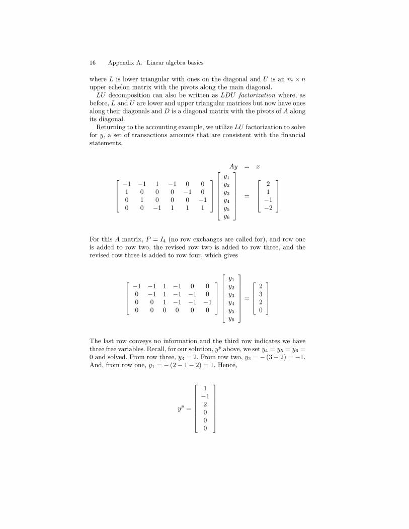
where L is lower triangular with ones on the diagonal and U is an m × nupper echelon matrix with the pivots along the main diagonal.LU decomposition can also be written as LDU factorization where, as
before, L and U are lower and upper triangular matrices but now have onesalong their diagonals and D is a diagonal matrix with the pivots of A alongits diagonal.Returning to the accounting example, we utilize LU factorization to solve
for y, a set of transactions amounts that are consistent with the financialstatements.
Ay = x−1 −1 1 −1 0 01 0 0 0 −1 00 1 0 0 0 −10 0 −1 1 1 1
y1
y2
y3
y4
y5
y6
=
21−1−2
For this A matrix, P = I4 (no row exchanges are called for), and row oneis added to row two, the revised row two is added to row three, and therevised row three is added to row four, which gives
−1 −1 1 −1 0 00 −1 1 −1 −1 00 0 1 −1 −1 −10 0 0 0 0 0
y1
y2
y3
y4
y5
y6
=
2320
The last row conveys no information and the third row indicates we havethree free variables. Recall, for our solution, yp above, we set y4 = y5 = y6 =0 and solved. From row three, y3 = 2. From row two, y2 = − (3− 2) = −1.And, from row one, y1 = − (2− 1− 2) = 1. Hence,
yp =
1−12000
A.4 Matrix decomposition and inverse operations 17
A.4.2 Cholesky decomposition
If the matrix A is symmetric, positive definite5 as well as nonsingular, thenwe have A = LDLT as U = LT . In this symmetric case, we identify an-other useful factorization, Cholesky decomposition. Cholesky decompositionwrites
A = ΓΓT
where Γ = LD12 and D
12 has the square root of the pivots on the diagonal.
Since A is positive definite, all of its pivots are positive and their squareroot is real so, in turn, Γ is real. Of course, we now have
Γ−1A = Γ−1ΓΓT
= ΓT
or
A(ΓT)−1
= ΓΓT(ΓT)−1
= Γ
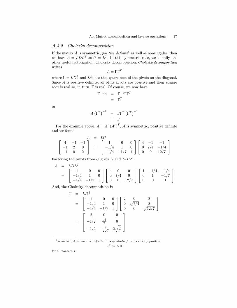
For the example above, A = Ar (Ar)T , A is symmetric, positive definite
and we found
A = LU 4 −1 −1−1 2 0−1 0 2
=
1 0 0−1/4 1 0−1/4 −1/7 1
4 −1 −10 7/4 −1/40 0 12/7
Factoring the pivots from U gives D and LDLT .
A = LDLT
=
1 0 0−1/4 1 0−1/4 −1/7 1
4 0 00 7/4 00 0 12/7
1 −1/4 −1/40 1 −1/70 0 1
And, the Cholesky decomposition is
Γ = LD12
=
1 0 0−1/4 1 0−1/4 −1/7 1
2 0 0
0√
7/4 0
0 0√
12/7
=
2 0 0
−1/2√
72 0
−1/2 − 12√
72√
37
5A matrix, A, is positive definite if its quadratic form is strictly positive
xTAx > 0
for all nonzero x.
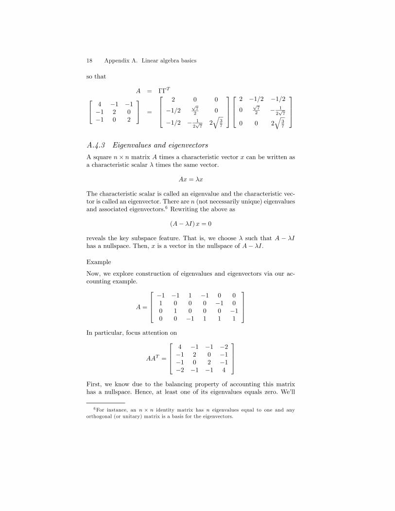
18 Appendix A. Linear algebra basics
so that
A = ΓΓT 4 −1 −1−1 2 0−1 0 2
=
2 0 0
−1/2√
72 0
−1/2 − 12√
72√
37
2 −1/2 −1/2
0√
72 − 1
2√
7
0 0 2√
37
A.4.3 Eigenvalues and eigenvectors
A square n× n matrix A times a characteristic vector x can be written asa characteristic scalar λ times the same vector.
Ax = λx
The characteristic scalar is called an eigenvalue and the characteristic vec-tor is called an eigenvector. There are n (not necessarily unique) eigenvaluesand associated eigenvectors.6 Rewriting the above as
(A− λI)x = 0
reveals the key subspace feature. That is, we choose λ such that A − λIhas a nullspace. Then, x is a vector in the nullspace of A− λI.
Example
Now, we explore construction of eigenvalues and eigenvectors via our ac-counting example.
A =
−1 −1 1 −1 0 01 0 0 0 −1 00 1 0 0 0 −10 0 −1 1 1 1
In particular, focus attention on
AAT =
4 −1 −1 −2−1 2 0 −1−1 0 2 −1−2 −1 −1 4
First, we know due to the balancing property of accounting this matrixhas a nullspace. Hence, at least one of its eigenvalues equals zero. We’ll
6For instance, an n × n identity matrix has n eigenvalues equal to one and anyorthogonal (or unitary) matrix is a basis for the eigenvectors.
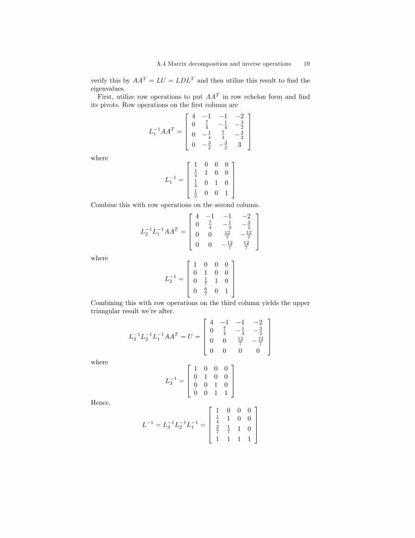
A.4 Matrix decomposition and inverse operations 19
verify this by AAT = LU = LDLT and then utilize this result to find theeigenvalues.First, utilize row operations to put AAT in row echelon form and find
its pivots. Row operations on the first column are
L−11 AAT =
4 −1 −1 −20 7
4 − 14 − 3
2
0 − 14
74 − 3
2
0 − 32 − 3
2 3
where
L−11 =
1 0 0 014 1 0 014 0 1 012 0 0 1
Combine this with row operations on the second column.
L−12 L−1
1 AAT =
4 −1 −1 −20 7
4 − 14 − 3
2
0 0 127 − 12
7
0 0 − 127
127
where
L−12 =
1 0 0 00 1 0 00 1
7 1 0
0 67 0 1
Combining this with row operations on the third column yields the uppertriangular result we’re after.
L−13 L−1
2 L−11 AAT = U =
4 −1 −1 −20 7
4 − 14 − 3
2
0 0 127 − 12
7
0 0 0 0
where
L−13 =
1 0 0 00 1 0 00 0 1 00 0 1 1
Hence,
L−1 = L−13 L−1
2 L−11 =
1 0 0 014 1 0 027
17 1 0
1 1 1 1
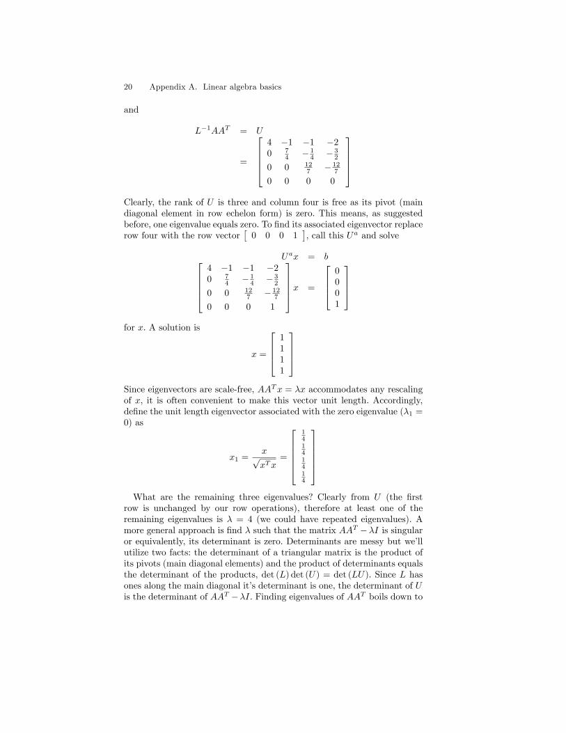
20 Appendix A. Linear algebra basics
and
L−1AAT = U
=
4 −1 −1 −20 7
4 − 14 − 3
2
0 0 127 − 12
7
0 0 0 0
Clearly, the rank of U is three and column four is free as its pivot (maindiagonal element in row echelon form) is zero. This means, as suggestedbefore, one eigenvalue equals zero. To find its associated eigenvector replacerow four with the row vector
[0 0 0 1
], call this Ua and solve
Uax = b4 −1 −1 −20 7
4 − 14 − 3
2
0 0 127 − 12
7
0 0 0 1
x =
0001
for x. A solution is
x =
1111
Since eigenvectors are scale-free, AATx = λx accommodates any rescalingof x, it is often convenient to make this vector unit length. Accordingly,define the unit length eigenvector associated with the zero eigenvalue (λ1 =0) as
x1 =x√xTx
=
14141414
What are the remaining three eigenvalues? Clearly from U (the first
row is unchanged by our row operations), therefore at least one of theremaining eigenvalues is λ = 4 (we could have repeated eigenvalues). Amore general approach is find λ such that the matrix AAT −λI is singularor equivalently, its determinant is zero. Determinants are messy but we’llutilize two facts: the determinant of a triangular matrix is the product ofits pivots (main diagonal elements) and the product of determinants equalsthe determinant of the products, det (L) det (U) = det (LU). Since L hasones along the main diagonal it’s determinant is one, the determinant of Uis the determinant of AAT −λI. Finding eigenvalues of AAT boils down to
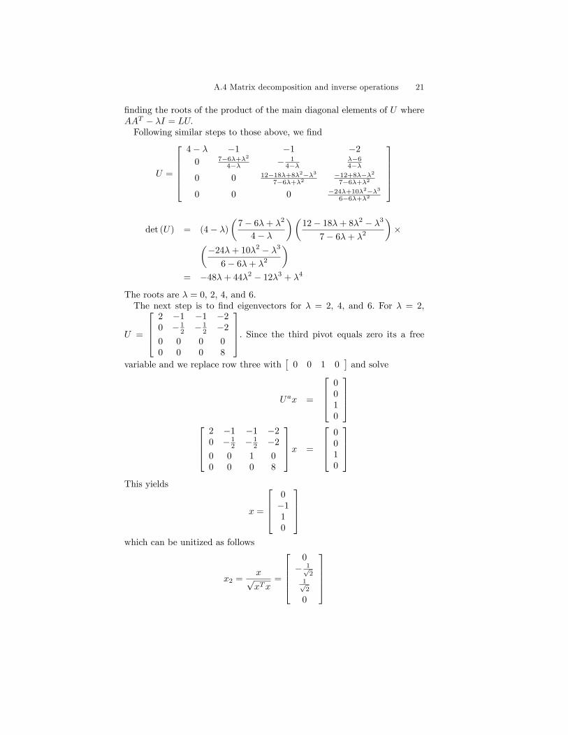
A.4 Matrix decomposition and inverse operations 21
finding the roots of the product of the main diagonal elements of U whereAAT − λI = LU.Following similar steps to those above, we find
U =
4− λ −1 −1 −2
0 7−6λ+λ2
4−λ − 14−λ
λ−64−λ
0 0 12−18λ+8λ2−λ37−6λ+λ2
−12+8λ−λ27−6λ+λ2
0 0 0 −24λ+10λ2−λ36−6λ+λ2
det (U) = (4− λ)
(7− 6λ+ λ2
4− λ
)(12− 18λ+ 8λ2 − λ3
7− 6λ+ λ2
)×(
−24λ+ 10λ2 − λ3
6− 6λ+ λ2
)= −48λ+ 44λ2 − 12λ3 + λ4
The roots are λ = 0, 2, 4, and 6.The next step is to find eigenvectors for λ = 2, 4, and 6. For λ = 2,
U =
2 −1 −1 −20 − 1
2 − 12 −2
0 0 0 00 0 0 8
. Since the third pivot equals zero its a freevariable and we replace row three with
[0 0 1 0
]and solve
Uax =
0010
2 −1 −1 −20 − 1
2 − 12 −2
0 0 1 00 0 0 8
x =
0010
This yields
x =
0−110
which can be unitized as follows
x2 =x√xTx
=
0− 1√
21√2
0
22 Appendix A. Linear algebra basics
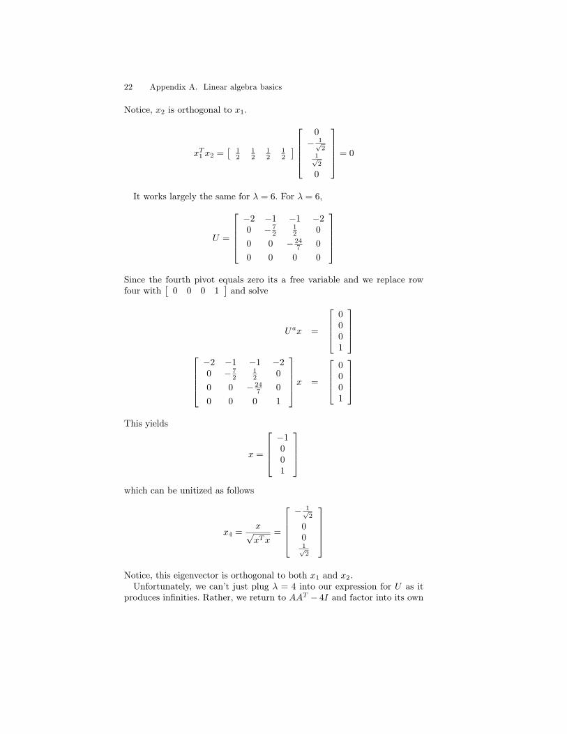
Notice, x2 is orthogonal to x1.
xT1 x2 =[
12
12
12
12
]
0− 1√
21√2
0
= 0
It works largely the same for λ = 6. For λ = 6,
U =
−2 −1 −1 −20 − 7
212 0
0 0 − 247 0
0 0 0 0
Since the fourth pivot equals zero its a free variable and we replace rowfour with
[0 0 0 1
]and solve
Uax =
0001
−2 −1 −1 −20 − 7
212 0
0 0 − 247 0
0 0 0 1
x =
0001
This yields
x =
−1001
which can be unitized as follows
x4 =x√xTx
=
− 1√
2
001√2
Notice, this eigenvector is orthogonal to both x1 and x2.Unfortunately, we can’t just plug λ = 4 into our expression for U as it
produces infinities. Rather, we return to AAT − 4I and factor into its own
A.4 Matrix decomposition and inverse operations 23
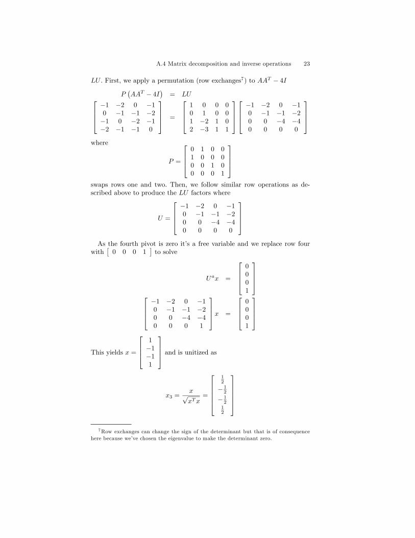
LU . First, we apply a permutation (row exchanges7) to AAT − 4I
P(AAT − 4I
)= LU
−1 −2 0 −10 −1 −1 −2−1 0 −2 −1−2 −1 −1 0
=
1 0 0 00 1 0 01 −2 1 02 −3 1 1
−1 −2 0 −10 −1 −1 −20 0 −4 −40 0 0 0
where
P =
0 1 0 01 0 0 00 0 1 00 0 0 1
swaps rows one and two. Then, we follow similar row operations as de-scribed above to produce the LU factors where
U =
−1 −2 0 −10 −1 −1 −20 0 −4 −40 0 0 0
As the fourth pivot is zero it’s a free variable and we replace row four
with[
0 0 0 1]to solve
Uax =
0001
−1 −2 0 −10 −1 −1 −20 0 −4 −40 0 0 1
x =
0001
This yields x =
1−1−11
and is unitized as
x3 =x√xTx
=
12
− 12
− 12
12
7Row exchanges can change the sign of the determinant but that is of consequence
here because we’ve chosen the eigenvalue to make the determinant zero.
24 Appendix A. Linear algebra basics
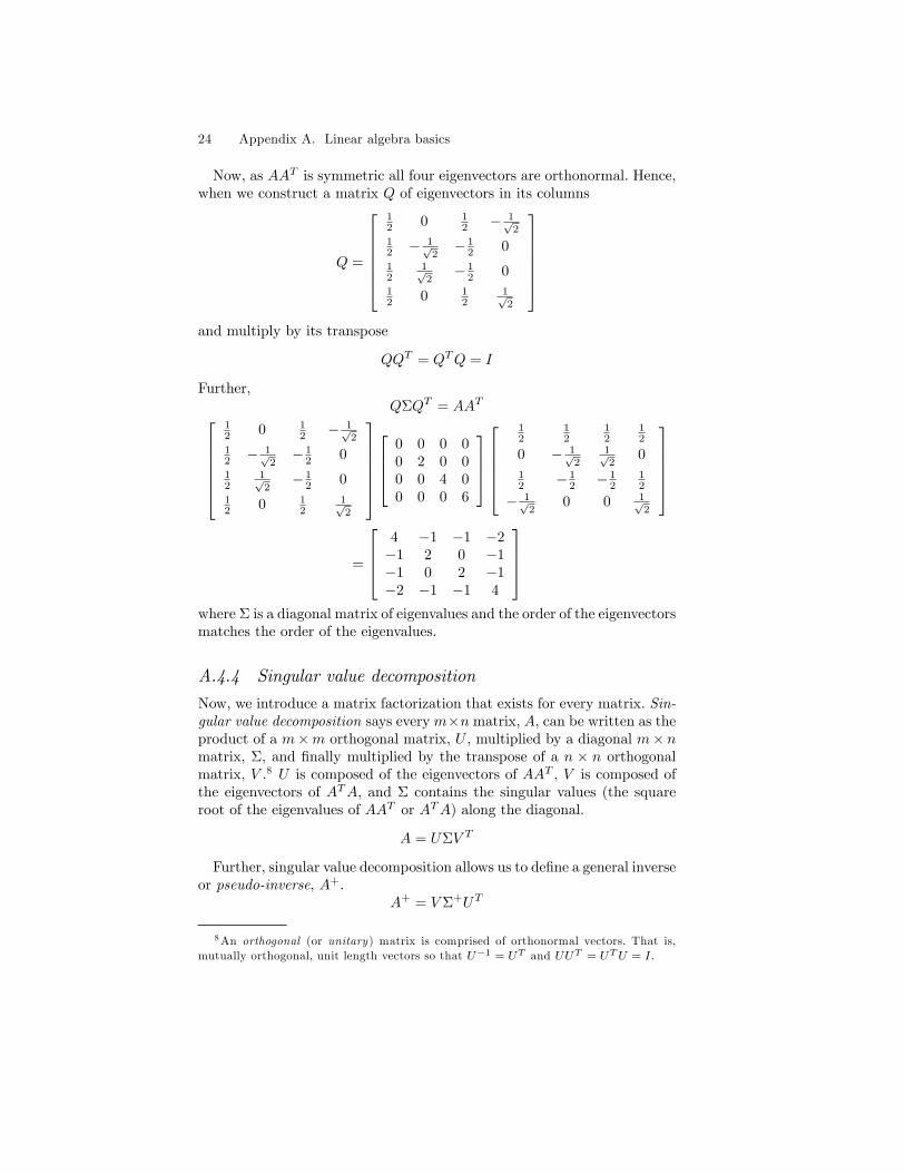
Now, as AAT is symmetric all four eigenvectors are orthonormal. Hence,when we construct a matrix Q of eigenvectors in its columns
Q =
12 0 1
2 − 1√2
12 − 1√
2− 1
2 0
12
1√2− 1
2 0
12 0 1
21√2
and multiply by its transpose
QQT = QTQ = I
Further,QΣQT = AAT
12 0 1
2 − 1√2
12 − 1√
2− 1
2 0
12
1√2− 1
2 0
12 0 1
21√2
0 0 0 00 2 0 00 0 4 00 0 0 6
12
12
12
12
0 − 1√2
1√2
0
12 − 1
2 − 12
12
− 1√2
0 0 1√2
=
4 −1 −1 −2−1 2 0 −1−1 0 2 −1−2 −1 −1 4
where Σ is a diagonal matrix of eigenvalues and the order of the eigenvectorsmatches the order of the eigenvalues.
A.4.4 Singular value decomposition
Now, we introduce a matrix factorization that exists for every matrix. Sin-gular value decomposition says everym×n matrix, A, can be written as theproduct of a m×m orthogonal matrix, U , multiplied by a diagonal m× nmatrix, Σ, and finally multiplied by the transpose of a n × n orthogonalmatrix, V .8 U is composed of the eigenvectors of AAT , V is composed ofthe eigenvectors of ATA, and Σ contains the singular values (the squareroot of the eigenvalues of AAT or ATA) along the diagonal.
A = UΣV T
Further, singular value decomposition allows us to define a general inverseor pseudo-inverse, A+.
A+ = V Σ+UT
8An orthogonal (or unitary ) matrix is comprised of orthonormal vectors. That is,mutually orthogonal, unit length vectors so that U−1 = UT and UUT = UTU = I.

A.4 Matrix decomposition and inverse operations 25
where Σ+ is an n×m diagonal matrix with nonzero elements equal to thereciprocal of those for Σ. This implies
AA+A = A
A+AA+ = A+
(A+A
)T= A+A
and (AA+
)T= AA+
Also, for the system of equations
Ay = x
the least squares solution is
yCS(A) = A+x
and AA+ is always the projection onto the columns of A. Hence,
AA+ = PA = A(ATA
)−1AT
if A has linearly independent columns. Or,
AT(AT)+
=(A+A
)T=
(V Σ+UTUΣV T
)T= V ΣTUTU
(Σ+)TV T
= A+A
= PAT = AT(AAT
)−1A
ifA has linearly independent rows (ifAT has linearly independent columns).For the accounting example, recall the row component is the consistent
solution to Ay = x that is only a linearly combination of the rows of A;that is, it is orthogonal to the nullspace. Utilizing the pseudo-inverse wehave
yRS(A) = AT(AT)+yp
= PAT yp
= (Ar)T(Ar (Ar)
T)−1
Aryp
= A+Ayp
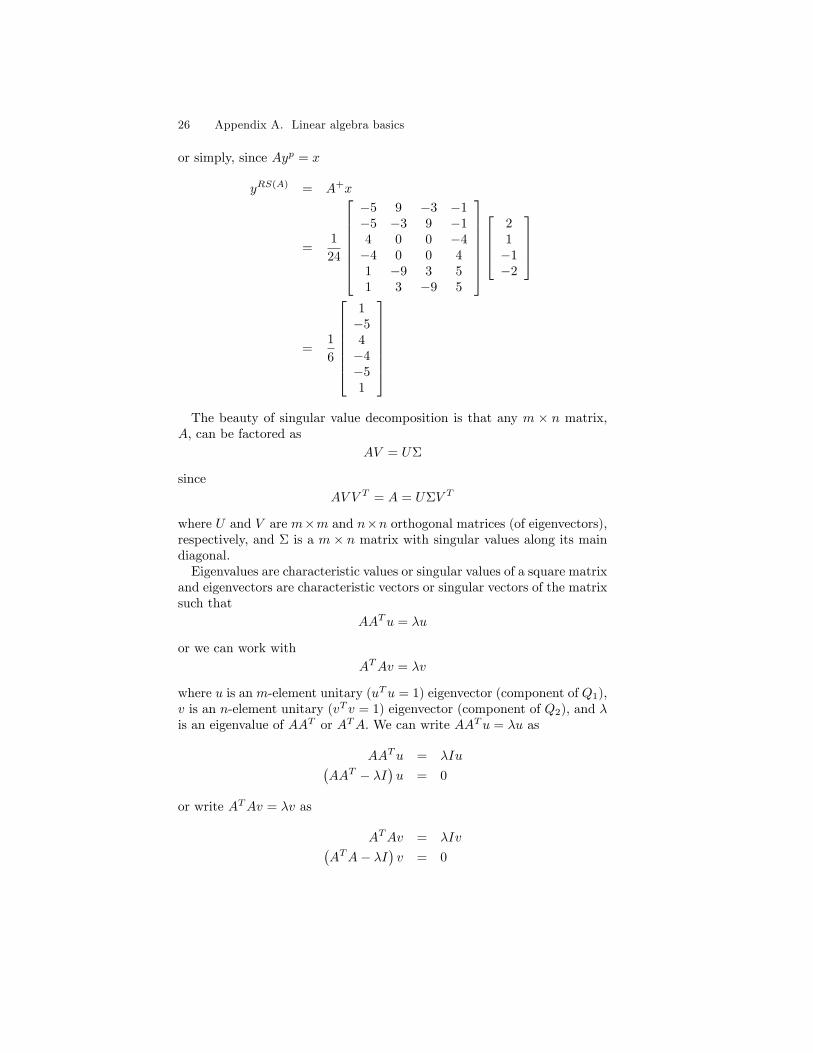
26 Appendix A. Linear algebra basics
or simply, since Ayp = x
yRS(A) = A+x
=1
24
−5 9 −3 −1−5 −3 9 −14 0 0 −4−4 0 0 41 −9 3 51 3 −9 5
21−1−2
=1
6
1−54−4−51
The beauty of singular value decomposition is that any m × n matrix,
A, can be factored asAV = UΣ
sinceAV V T = A = UΣV T
where U and V are m×m and n×n orthogonal matrices (of eigenvectors),respectively, and Σ is a m × n matrix with singular values along its maindiagonal.Eigenvalues are characteristic values or singular values of a square matrix
and eigenvectors are characteristic vectors or singular vectors of the matrixsuch that
AATu = λu
or we can work withATAv = λv
where u is an m-element unitary (uTu = 1) eigenvector (component of Q1),v is an n-element unitary (vT v = 1) eigenvector (component of Q2), and λis an eigenvalue of AAT or ATA. We can write AATu = λu as
AATu = λIu(AAT − λI
)u = 0
or write ATAv = λv as
ATAv = λIv(ATA− λI
)v = 0
A.4 Matrix decomposition and inverse operations 27
then solve for unitary vectors u, v, and and roots λ. For instance, once wehave λi and ui in hand. We find vi by
uTi A = λivi
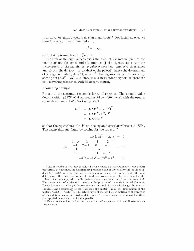
such that vi is unit length, vTi vi = 1.The sum of the eigenvalues equals the trace of the matrix (sum of the
main diagonal elements) and the product of the eigenvalues equals thedeterminant of the matrix. A singular matrix has some zero eigenvaluesand pivots (the det (A) = ±[product of the pivots]), hence the determinantof a singular matrix, det (A), is zero.9 The eigenvalues can be found bysolving det
(AAT − λI
)= 0. Since this is an m order polynomial, there are
m eigenvalues associated with an m×m matrix.
Accounting example
Return to the accounting example for an illustration. The singular valuedecomposition (SVD) of A proceeds as follows. We’ll work with the square,symmetric matrix AAT . Notice, by SVD,
AAT = UΣV T(UΣV T
)T= UΣV TV ΣTUT
= UΣΣTUT
so that the eigenvalues of AAT are the squared singular values of A, ΣΣT .The eigenvalues are found by solving for the roots of10
det(AAT − λIm
)= 0
det
4− λ −1 −1 −2−1 2− λ 0 −1−1 0 2− λ −1−2 −1 −1 4− λ
= 0
−48λ+ 44λ2 − 12λ3 + λ4 = 0
9The determinant is a value associated with a square matrix with many (some useful)properties. For instance, the determinant provides a test of invertibility (linear indepen-dence). If det (A) = 0, then the matrix is singular and the inverse doesn’t exist; otherwisedet (A) 6= 0, the matrix is nonsingular and the inverse exists. The determinant is thevolume of a parallelpiped in n-dimensions where the edges come from the rows of A.The determinant of a triangular matrix is the product of the main diagonal elements.Determinants are unchanged by row eliminations and their sign is changed by row ex-changes. The determinant of the transpose of a matrix equals the determinant of thematrix, det (A) = det
(AT
). The determinant of the product of matrices is the product
of their determinants, det (AB) = det (A) det (B). Some useful determinant identitiesare reported in section five of the appendix.10Below we show how to find the determinant of a square matrix and illustrate with
this example.
28 Appendix A. Linear algebra basics
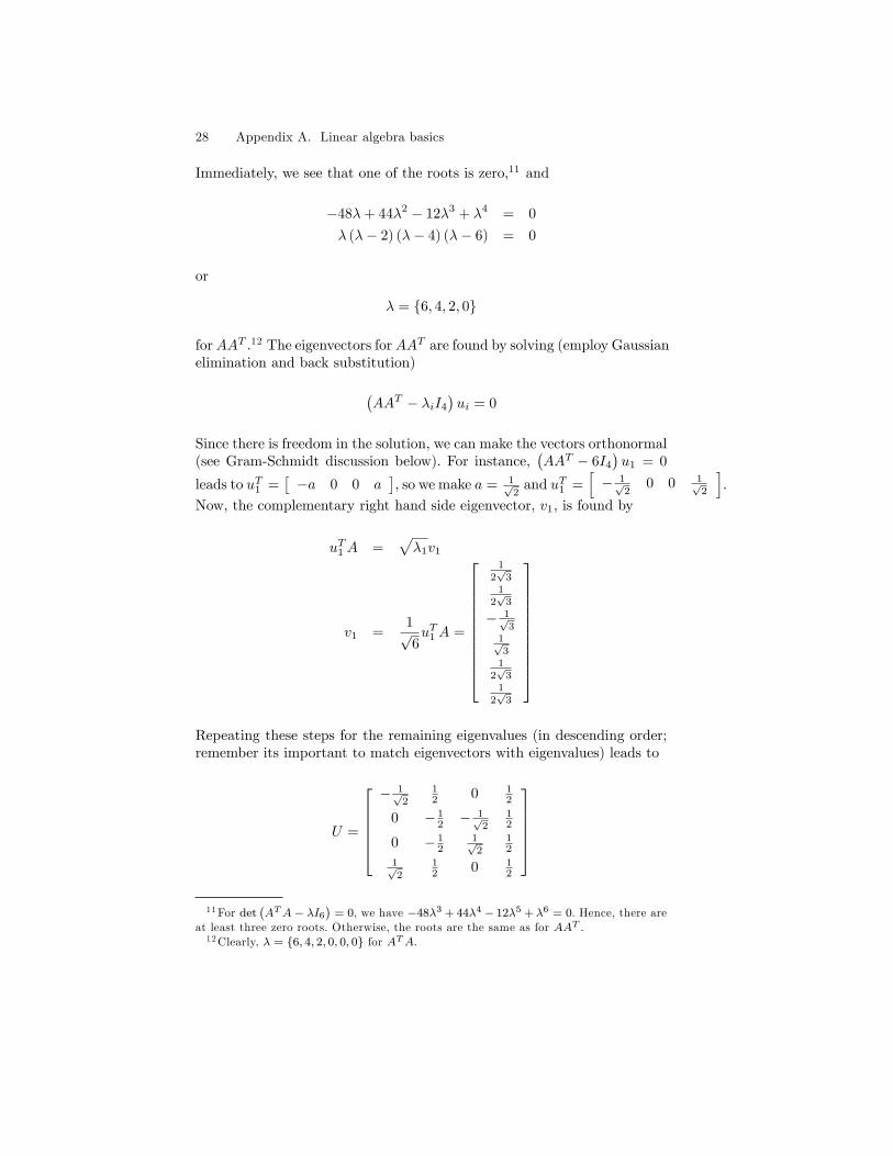
Immediately, we see that one of the roots is zero,11 and
−48λ+ 44λ2 − 12λ3 + λ4 = 0
λ (λ− 2) (λ− 4) (λ− 6) = 0
or
λ = {6, 4, 2, 0}
forAAT .12 The eigenvectors forAAT are found by solving (employ Gaussianelimination and back substitution)
(AAT − λiI4
)ui = 0
Since there is freedom in the solution, we can make the vectors orthonormal(see Gram-Schmidt discussion below). For instance,
(AAT − 6I4
)u1 = 0
leads to uT1 =[−a 0 0 a
], so we make a = 1√
2and uT1 =
[− 1√
20 0 1√
2
].
Now, the complementary right hand side eigenvector, v1, is found by
uT1 A =√λ1v1
v1 =1√6uT1 A =
12√
31
2√
3
− 1√3
1√3
12√
31
2√
3
Repeating these steps for the remaining eigenvalues (in descending order;remember its important to match eigenvectors with eigenvalues) leads to
U =
− 1√
212 0 1
2
0 − 12 − 1√
212
0 − 12
1√2
12
1√2
12 0 1
2
11For det
(ATA− λI6
)= 0, we have −48λ3 +44λ4 − 12λ5 + λ6 = 0. Hence, there are
at least three zero roots. Otherwise, the roots are the same as for AAT .12Clearly, λ = {6, 4, 2, 0, 0, 0} for ATA.
A.4 Matrix decomposition and inverse operations 29
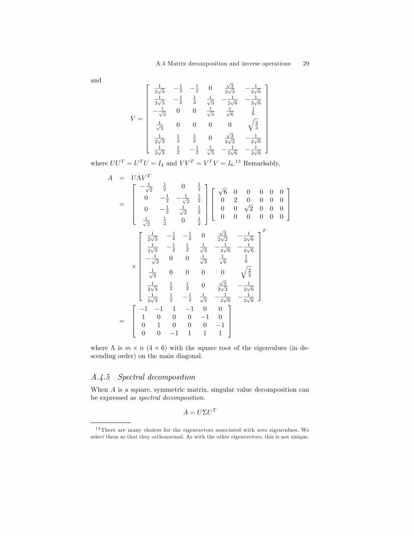
and
V =
12√
3− 1
2 − 12 0
√3
2√
2− 1
2√
61
2√
3− 1
212
1√3− 1
2√
6− 1
2√
6
− 1√3
0 0 1√3
1√6
16
1√3
0 0 0 0√
23
12√
312
12 0
√3
2√
2− 1
2√
61
2√
312 − 1
21√3− 1
2√
6− 1
2√
6
where UUT = UTU = I4 and V V T = V TV = I6.13 Remarkably,
A = UΛV T
=
− 1√
212 0 1
2
0 − 12 − 1√
212
0 − 12
1√2
12
1√2
12 0 1
2
√
6 0 0 0 0 00 2 0 0 0 0
0 0√
2 0 0 00 0 0 0 0 0
×
12√
3− 1
2 − 12 0
√3
2√
2− 1
2√
61
2√
3− 1
212
1√3− 1
2√
6− 1
2√
6
− 1√3
0 0 1√3
1√6
16
1√3
0 0 0 0√
23
12√
312
12 0
√3
2√
2− 1
2√
61
2√
312 − 1
21√3− 1
2√
6− 1
2√
6
T
=
−1 −1 1 −1 0 01 0 0 0 −1 00 1 0 0 0 −10 0 −1 1 1 1
where Λ is m × n (4 × 6) with the square root of the eigenvalues (in de-scending order) on the main diagonal.
A.4.5 Spectral decomposition
When A is a square, symmetric matrix, singular value decomposition canbe expressed as spectral decomposition.
A = UΣUT
13There are many choices for the eigenvectors associated with zero eigenvalues. Weselect them so that they orthonormal. As with the other eigenvectors, this is not unique.
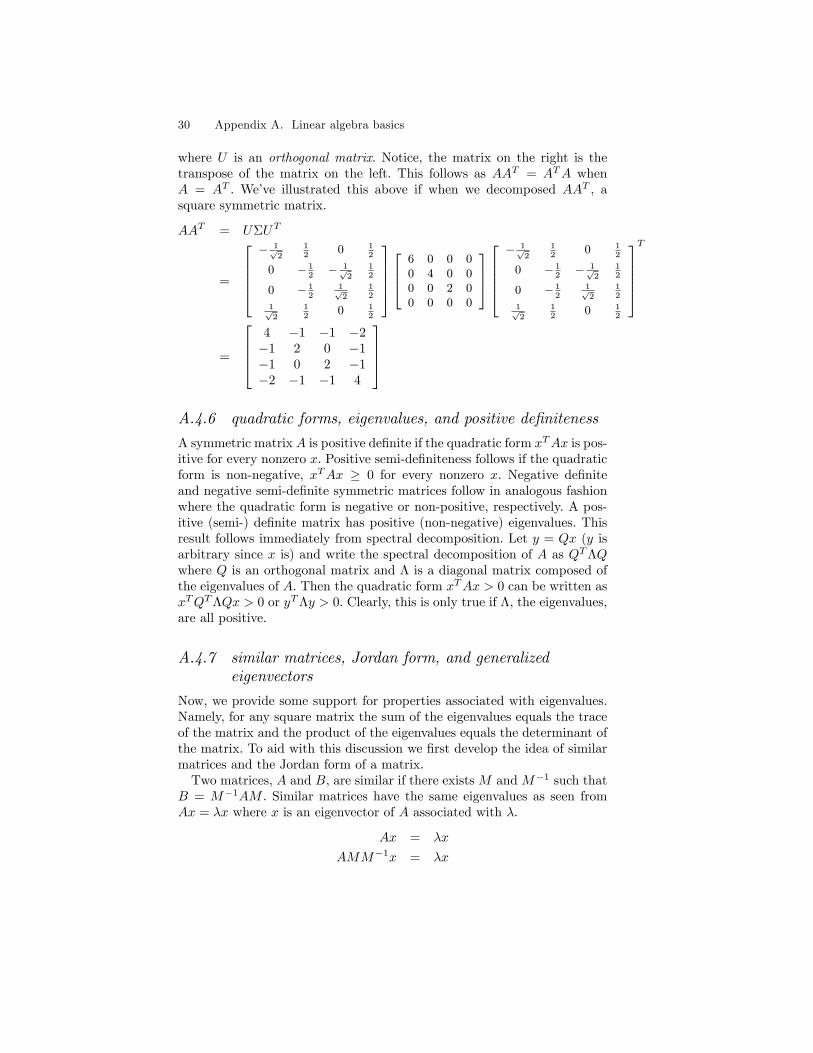
30 Appendix A. Linear algebra basics
where U is an orthogonal matrix. Notice, the matrix on the right is thetranspose of the matrix on the left. This follows as AAT = ATA whenA = AT . We’ve illustrated this above if when we decomposed AAT , asquare symmetric matrix.
AAT = UΣUT
=
− 1√
2
12
0 12
0 − 12
− 1√2
12
0 − 12
1√2
12
1√2
12
0 12
6 0 0 00 4 0 00 0 2 00 0 0 0
− 1√
2
12
0 12
0 − 12
− 1√2
12
0 − 12
1√2
12
1√2
12
0 12
T
=
4 −1 −1 −2−1 2 0 −1−1 0 2 −1−2 −1 −1 4
A.4.6 quadratic forms, eigenvalues, and positive definiteness
A symmetric matrix A is positive definite if the quadratic form xTAx is pos-itive for every nonzero x. Positive semi-definiteness follows if the quadraticform is non-negative, xTAx ≥ 0 for every nonzero x. Negative definiteand negative semi-definite symmetric matrices follow in analogous fashionwhere the quadratic form is negative or non-positive, respectively. A pos-itive (semi-) definite matrix has positive (non-negative) eigenvalues. Thisresult follows immediately from spectral decomposition. Let y = Qx (y isarbitrary since x is) and write the spectral decomposition of A as QTΛQwhere Q is an orthogonal matrix and Λ is a diagonal matrix composed ofthe eigenvalues of A. Then the quadratic form xTAx > 0 can be written asxTQTΛQx > 0 or yTΛy > 0. Clearly, this is only true if Λ, the eigenvalues,are all positive.
A.4.7 similar matrices, Jordan form, and generalizedeigenvectors
Now, we provide some support for properties associated with eigenvalues.Namely, for any square matrix the sum of the eigenvalues equals the traceof the matrix and the product of the eigenvalues equals the determinant ofthe matrix. To aid with this discussion we first develop the idea of similarmatrices and the Jordan form of a matrix.Two matrices, A and B, are similar if there existsM andM−1 such that
B = M−1AM . Similar matrices have the same eigenvalues as seen fromAx = λx where x is an eigenvector of A associated with λ.
Ax = λx
AMM−1x = λx
A.4 Matrix decomposition and inverse operations 31
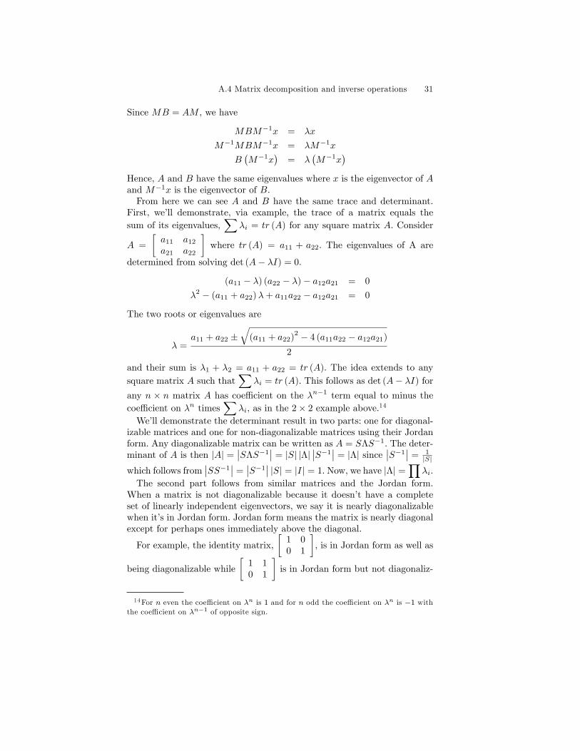
Since MB = AM , we have
MBM−1x = λx
M−1MBM−1x = λM−1x
B(M−1x
)= λ
(M−1x
)Hence, A and B have the same eigenvalues where x is the eigenvector of Aand M−1x is the eigenvector of B.From here we can see A and B have the same trace and determinant.
First, we’ll demonstrate, via example, the trace of a matrix equals thesum of its eigenvalues,
∑λi = tr (A) for any square matrix A. Consider
A =
[a11 a12
a21 a22
]where tr (A) = a11 + a22. The eigenvalues of A are
determined from solving det (A− λI) = 0.
(a11 − λ) (a22 − λ)− a12a21 = 0
λ2 − (a11 + a22)λ+ a11a22 − a12a21 = 0
The two roots or eigenvalues are
λ =a11 + a22 ±
√(a11 + a22)
2 − 4 (a11a22 − a12a21)
2
and their sum is λ1 + λ2 = a11 + a22 = tr (A). The idea extends to anysquare matrix A such that
∑λi = tr (A). This follows as det (A− λI) for
any n × n matrix A has coeffi cient on the λn−1 term equal to minus thecoeffi cient on λn times
∑λi, as in the 2× 2 example above.14
We’ll demonstrate the determinant result in two parts: one for diagonal-izable matrices and one for non-diagonalizable matrices using their Jordanform. Any diagonalizable matrix can be written as A = SΛS−1. The deter-minant of A is then |A| =
∣∣SΛS−1∣∣ = |S| |Λ|
∣∣S−1∣∣ = |Λ| since
∣∣S−1∣∣ = 1
|S|
which follows from∣∣SS−1
∣∣ =∣∣S−1
∣∣ |S| = |I| = 1. Now, we have |Λ| =∏
λi.The second part follows from similar matrices and the Jordan form.
When a matrix is not diagonalizable because it doesn’t have a completeset of linearly independent eigenvectors, we say it is nearly diagonalizablewhen it’s in Jordan form. Jordan form means the matrix is nearly diagonalexcept for perhaps ones immediately above the diagonal.
For example, the identity matrix,[
1 00 1
], is in Jordan form as well as
being diagonalizable while[
1 10 1
]is in Jordan form but not diagonaliz-
14For n even the coeffi cient on λn is 1 and for n odd the coeffi cient on λn is −1 withthe coeffi cient on λn−1 of opposite sign.
32 Appendix A. Linear algebra basics
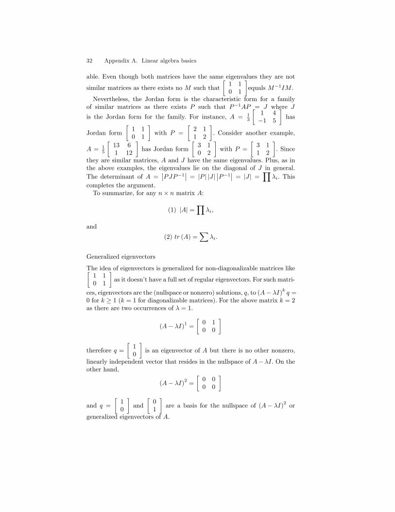
able. Even though both matrices have the same eigenvalues they are not
similar matrices as there exists no M such that[
1 10 1
]equals M−1IM .
Nevertheless, the Jordan form is the characteristic form for a familyof similar matrices as there exists P such that P−1AP = J where J
is the Jordan form for the family. For instance, A = 13
[1 4−1 5
]has
Jordan form[
1 10 1
]with P =
[2 11 2
]. Consider another example,
A = 15
[13 61 12
]has Jordan form
[3 10 2
]with P =
[3 11 2
]. Since
they are similar matrices, A and J have the same eigenvalues. Plus, as inthe above examples, the eigenvalues lie on the diagonal of J in general.The determinant of A =
∣∣PJP−1∣∣ = |P | |J |
∣∣P−1∣∣ = |J | =
∏λi. This
completes the argument.To summarize, for any n× n matrix A:
(1) |A| =∏
λi,
and
(2) tr (A) =∑
λi.
Generalized eigenvectors
The idea of eigenvectors is generalized for non-diagonalizable matrices like[1 10 1
]as it doesn’t have a full set of regular eigenvectors. For such matri-
ces, eigenvectors are the (nullspace or nonzero) solutions, q, to (A− λI)kq =
0 for k ≥ 1 (k = 1 for diagonalizable matrices). For the above matrix k = 2as there are two occurrences of λ = 1.
(A− λI)1
=
[0 10 0
]
therefore q =
[10
]is an eigenvector of A but there is no other nonzero,
linearly independent vector that resides in the nullspace of A− λI. On theother hand,
(A− λI)2
=
[0 00 0
]
and q =
[10
]and
[01
]are a basis for the nullspace of (A− λI)
2 or
generalized eigenvectors of A.
A.5 Gram-Schmidt construction of an orthogonal matrix 33
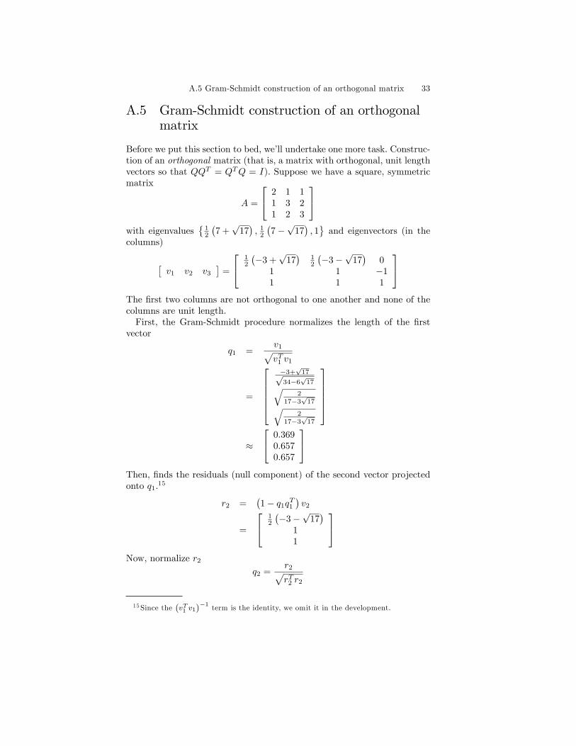
A.5 Gram-Schmidt construction of an orthogonalmatrix
Before we put this section to bed, we’ll undertake one more task. Construc-tion of an orthogonal matrix (that is, a matrix with orthogonal, unit lengthvectors so that QQT = QTQ = I). Suppose we have a square, symmetricmatrix
A =
2 1 11 3 21 2 3
with eigenvalues
{12
(7 +√
17), 1
2
(7−√
17), 1}and eigenvectors (in the
columns)
[v1 v2 v3
]=
12
(−3 +
√17)
12
(−3−
√17)
01 1 −11 1 1
The first two columns are not orthogonal to one another and none of thecolumns are unit length.First, the Gram-Schmidt procedure normalizes the length of the first
vector
q1 =v1√vT1 v1
=
−3+
√17√
34−6√
17√2
17−3√
17√2
17−3√
17
≈
0.3690.6570.657
Then, finds the residuals (null component) of the second vector projectedonto q1.15
r2 =(1− q1q
T1
)v2
=
12
(−3−
√17)
11
Now, normalize r2
q2 =r2√rT2 r2
15Since the(vT1 v1
)−1 term is the identity, we omit it in the development.
34 Appendix A. Linear algebra basics
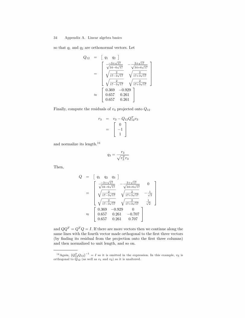
so that q1 and q2 are orthonormal vectors. Let
Q12 =[q1 q2
]
=
−3+
√17√
34−6√
17− 3+
√17√
34+6√
17√2
17−3√
17
√2
17+3√
17√2
17−3√
17
√2
17+3√
17
≈
0.369 −0.9290.657 0.2610.657 0.261
Finally, compute the residuals of v3 projected onto Q12
r3 = v3 −Q12QT12v3
=
0−11
and normalize its length.16
q3 =r3√rT3 r3
Then,
Q =[q1 q2 q3
]
=
−3+
√17√
34−6√
17− 3+
√17√
34+6√
170√
217−3
√17
√2
17+3√
17− 1√
2√2
17−3√
17
√2
17+3√
171√2
≈
0.369 −0.929 00.657 0.261 −0.7070.657 0.261 0.707
and QQT = QTQ = I. If there are more vectors then we continue along thesame lines with the fourth vector made orthogonal to the first three vectors(by finding its residual from the projection onto the first three columns)and then normalized to unit length, and so on.
16Again,(QT12Q12
)−1= I so it is omitted in the expression. In this example, v3 is
orthogonal to Q12 (as well as v1 and v2) so it is unaltered.
A.5 Gram-Schmidt construction of an orthogonal matrix 35
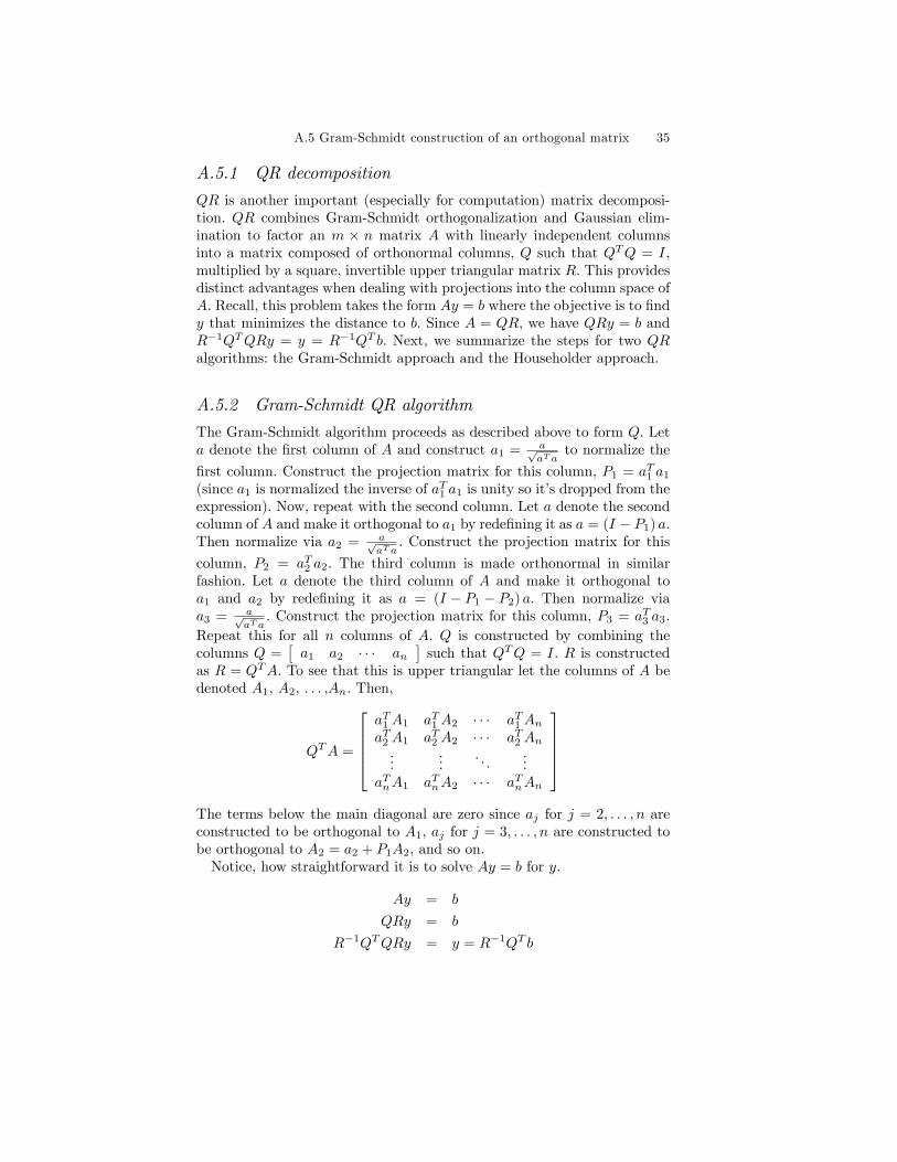
A.5.1 QR decomposition
QR is another important (especially for computation) matrix decomposi-tion. QR combines Gram-Schmidt orthogonalization and Gaussian elim-ination to factor an m × n matrix A with linearly independent columnsinto a matrix composed of orthonormal columns, Q such that QTQ = I,multiplied by a square, invertible upper triangular matrix R. This providesdistinct advantages when dealing with projections into the column space ofA. Recall, this problem takes the form Ay = b where the objective is to findy that minimizes the distance to b. Since A = QR, we have QRy = b andR−1QTQRy = y = R−1QT b. Next, we summarize the steps for two QRalgorithms: the Gram-Schmidt approach and the Householder approach.
A.5.2 Gram-Schmidt QR algorithm
The Gram-Schmidt algorithm proceeds as described above to form Q. Leta denote the first column of A and construct a1 = a√
aT ato normalize the
first column. Construct the projection matrix for this column, P1 = aT1 a1
(since a1 is normalized the inverse of aT1 a1 is unity so it’s dropped from theexpression). Now, repeat with the second column. Let a denote the secondcolumn of A and make it orthogonal to a1 by redefining it as a = (I − P1) a.Then normalize via a2 = a√
aT a. Construct the projection matrix for this
column, P2 = aT2 a2. The third column is made orthonormal in similarfashion. Let a denote the third column of A and make it orthogonal toa1 and a2 by redefining it as a = (I − P1 − P2) a. Then normalize viaa3 = a√
aT a. Construct the projection matrix for this column, P3 = aT3 a3.
Repeat this for all n columns of A. Q is constructed by combining thecolumns Q =
[a1 a2 · · · an
]such that QTQ = I. R is constructed
as R = QTA. To see that this is upper triangular let the columns of A bedenoted A1, A2, . . . ,An. Then,
QTA =
aT1 A1 aT1 A2 · · · aT1 AnaT2 A1 aT2 A2 · · · aT2 An...
.... . .
...aTnA1 aTnA2 · · · aTnAn
The terms below the main diagonal are zero since aj for j = 2, . . . , n areconstructed to be orthogonal to A1, aj for j = 3, . . . , n are constructed tobe orthogonal to A2 = a2 + P1A2, and so on.Notice, how straightforward it is to solve Ay = b for y.
Ay = b
QRy = b
R−1QTQRy = y = R−1QT b
36 Appendix A. Linear algebra basics
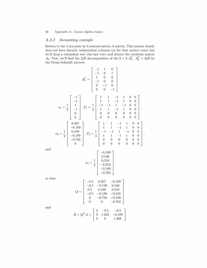
A.5.3 Accounting example
Return to the 4 accounts by 6 journal entries A matrix. This matrix clearlydoes not have linearly independent columns (or for that matter rows) butwe’ll drop a redundant row (the last row) and denote the resultant matrixA0. Now, we’ll find the QR decomposition of the 6 × 3 AT0 , A
T0 = QR by
the Gram-Schmidt process.
AT0 =
−1 1 0−1 0 11 0 0−1 0 00 −1 00 0 −1
a1 =1
2
−1−11−100
, P1 =1
4
1 1 −1 1 0 01 1 −1 1 0 0−1 −1 1 −1 0 01 1 −1 1 0 00 0 0 0 0 00 0 0 0 0 0
,
a2 =1
2
0.567−0.1890.189−0.189−0.756
0
, P2 =1
4
1 1 −1 1 0 01 1 −1 1 0 0−1 −1 1 −1 0 01 1 −1 1 0 00 0 0 0 0 00 0 0 0 0 0
,
and
a3 =1
2
−0.1090.5460.218−0.218−0.109−0.764
so that
Q =
−0.5 0.567 −0.109−0.5 −0.189 0.5460.5 0.189 0.218−0.5 −0.189 −0.218
0 −0.756 −0.1090 0 −0.764
and
R = QTA =
2 −0.5 −0.50 1.323 −0.1890 0 1.309
A.5 Gram-Schmidt construction of an orthogonal matrix 37
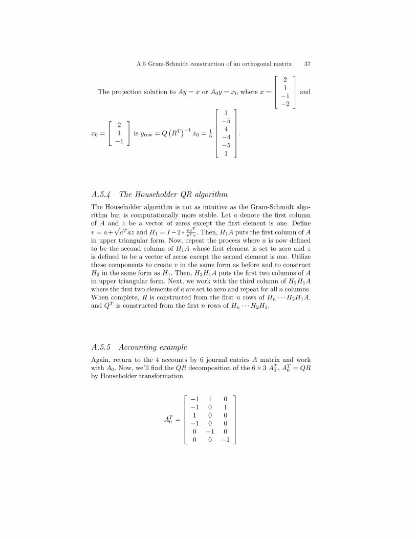
The projection solution to Ay = x or A0y = x0 where x =
21−1−2
and
x0 =
21−1
is yrow = Q(RT)−1
x0 = 16
1−54−4−51
.
A.5.4 The Householder QR algorithm
The Householder algorithm is not as intuitive as the Gram-Schmidt algo-rithm but is computationally more stable. Let a denote the first columnof A and z be a vector of zeros except the first element is one. Definev = a+
√aTaz and H1 = I−2∗ vvT
vT v. Then, H1A puts the first column of A
in upper triangular form. Now, repeat the process where a is now definedto be the second column of H1A whose first element is set to zero and zis defined to be a vector of zeros except the second element is one. Utilizethese components to create v in the same form as before and to constructH2 in the same form as H1. Then, H2H1A puts the first two columns of Ain upper triangular form. Next, we work with the third column of H2H1Awhere the first two elements of a are set to zero and repeat for all n columns.When complete, R is constructed from the first n rows of Hn · · ·H2H1A.and QT is constructed from the first n rows of Hn · · ·H2H1.
A.5.5 Accounting example
Again, return to the 4 accounts by 6 journal entries A matrix and workwith A0. Now, we’ll find the QR decomposition of the 6× 3 AT0 , A
T0 = QR
by Householder transformation.
AT0 =
−1 1 0−1 0 11 0 0−1 0 00 −1 00 0 −1
38 Appendix A. Linear algebra basics
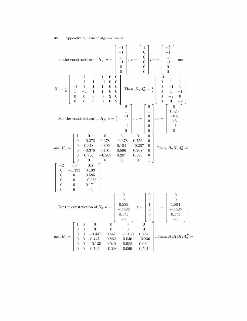
In the construction of H1, a =
−1−11−100
, z =
100000
, v =
− 1
2−11−100
, and
H1 = 12
1 1 −1 1 0 01 1 1 −1 0 0−1 1 1 1 0 01 −1 1 1 0 00 0 0 0 2 00 0 0 0 0 2
. Then,H1AT0 = 1
2
−4 1 10 1 10 −1 10 1 −10 −2 00 0 −2
.
For the construction of H2, a = 12
01−11−20
, z =
010000
, v =
0
1.823−0.50.5−10
,
andH2 =
1 0 0 0 0 00 −0.378 0.378 −0.378 0.756 00 0.378 0.896 0.104 −0.207 00 −0.378 0.104 0.896 0.207 00 0.756 −0.207 0.207 0.585 00 0 0 0 0 1
. Then,H2H1AT0 =
−2 0.5 0.50 −1.323 0.1890 0 0.5850 0 −0.5850 0 0.1710 0 −1
.
For the construction ofH3, a =
00
0.585−0.5850.171−1
, z =
001000
, v =
00
1.894−0.5850.171−1
,
andH3 =
1 0 0 0 0 00 0 0 0 0 00 0 −0.447 0.447 −0.130 0.7640 0 0.447 0.862 0.040 −0.2360 0 −0.130 0.040 0.988 0.0690 0 0.764 −0.236 0.069 0.597
. Then,H3H2H1AT0 =
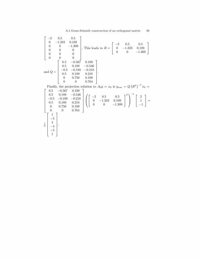
A.5 Gram-Schmidt construction of an orthogonal matrix 39−2 0.5 0.50 −1.323 0.1890 0 −1.3090 0 00 0 00 0 0
. This leads to R =
−2 0.5 0.50 −1.323 0.1890 0 −1.309
and Q =
0.5 −0.567 0.1090.5 0.189 −0.546−0.5 −0.189 −0.2180.5 0.189 0.2180 0.756 0.1090 0 0.764
.Finally, the projection solution to A0y = x0 is yrow = Q
(RT)−1
x0 =0.5 −0.567 0.1090.5 0.189 −0.546−0.5 −0.189 −0.2180.5 0.189 0.2180 0.756 0.1090 0 0.764
−2 0.5 0.5
0 −1.323 0.1890 0 −1.309
T−1 2
1−1
=
16
1−54−4−51
.
40 Appendix A. Linear algebra basics
A.6 Computing eigenvalues
As discussed above, eigenvalues are the characteristic values that ensure(A− λI) has a nullspace for square matrix A. That is, (A− λI)x = 0where x is an eigenvector. If an eigenvector can be identified such thatAx = λx then the constant, λ, is an associated eigenvalue. For instance,if the rows of A have the same sum then x = ι (a vector of ones) and λequals the sum of any row of A.Further, since the sum of the eigenvalues equals the trace of the matrix
and the product of the eigenvalues equals the determinant of the matrix,finding the eigenvalues for small matrices is relatively simple. For instance,eigenvalues of a 2× 2 matrix can be found by solving
λ1 + λ2 = tr (A)
λ1λ2 = det (A)
Alternatively, we can solve the roots or zeroes of the characteristic polyno-mial. That is, det (A− λI) = 0.
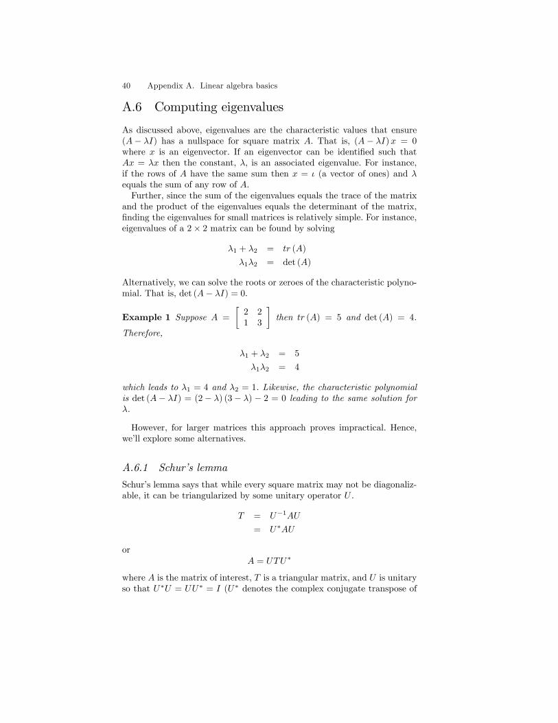
Example 1 Suppose A =
[2 21 3
]then tr (A) = 5 and det (A) = 4.
Therefore,
λ1 + λ2 = 5
λ1λ2 = 4
which leads to λ1 = 4 and λ2 = 1. Likewise, the characteristic polynomialis det (A− λI) = (2− λ) (3− λ) − 2 = 0 leading to the same solution forλ.
However, for larger matrices this approach proves impractical. Hence,we’ll explore some alternatives.
A.6.1 Schur’s lemma
Schur’s lemma says that while every square matrix may not be diagonaliz-able, it can be triangularized by some unitary operator U .
T = U−1AU
= U∗AU
orA = UTU∗
where A is the matrix of interest, T is a triangular matrix, and U is unitaryso that U∗U = UU∗ = I (U∗ denotes the complex conjugate transpose of
A.6 Computing eigenvalues 41
U). Further, since T and A are similar matrices they have the same eigen-values and the eigenvalues reside on the main diagonal of T . To see they aresimilar matrices recognize they have the same characteristic polynomial.
det(A− λI) = det (T − λI)
= det (U∗AU − λI)
= det (U∗AU − λU∗IU)
= det (U∗(A− λI)U)
= det (U∗) det (A− λI) det (U)
= 1 det (A− λI) 1
= det (A− λI)
Before discussing construction of T , we introduce some eigenvalue construc-tion algorithms.
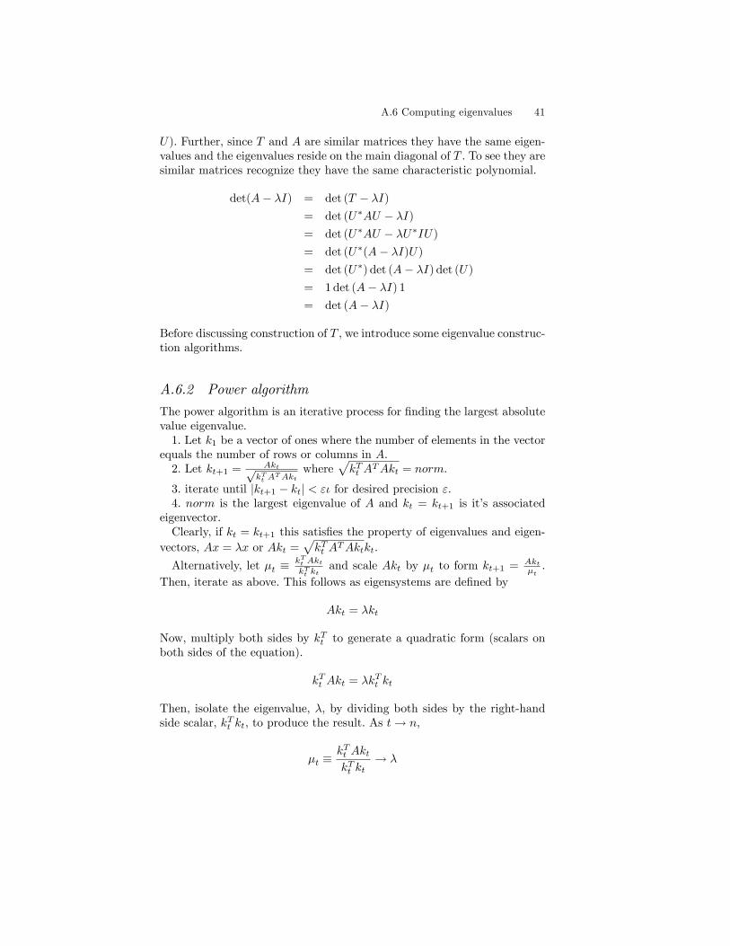
A.6.2 Power algorithm
The power algorithm is an iterative process for finding the largest absolutevalue eigenvalue.1. Let k1 be a vector of ones where the number of elements in the vector
equals the number of rows or columns in A.2. Let kt+1 = Akt√
kTt ATAkt
where√kTt A
TAkt = norm.
3. iterate until |kt+1 − kt| < ει for desired precision ε.4. norm is the largest eigenvalue of A and kt = kt+1 is it’s associated
eigenvector.Clearly, if kt = kt+1 this satisfies the property of eigenvalues and eigen-
vectors, Ax = λx or Akt =√kTt A
TAktkt.
Alternatively, let µt ≡kTt AktkTt kt
and scale Akt by µt to form kt+1 = Aktµt.
Then, iterate as above. This follows as eigensystems are defined by
Akt = λkt
Now, multiply both sides by kTt to generate a quadratic form (scalars onboth sides of the equation).
kTt Akt = λkTt kt
Then, isolate the eigenvalue, λ, by dividing both sides by the right-handside scalar, kTt kt, to produce the result. As t→ n,
µt ≡kTt AktkTt kt
→ λ
42 Appendix A. Linear algebra basics
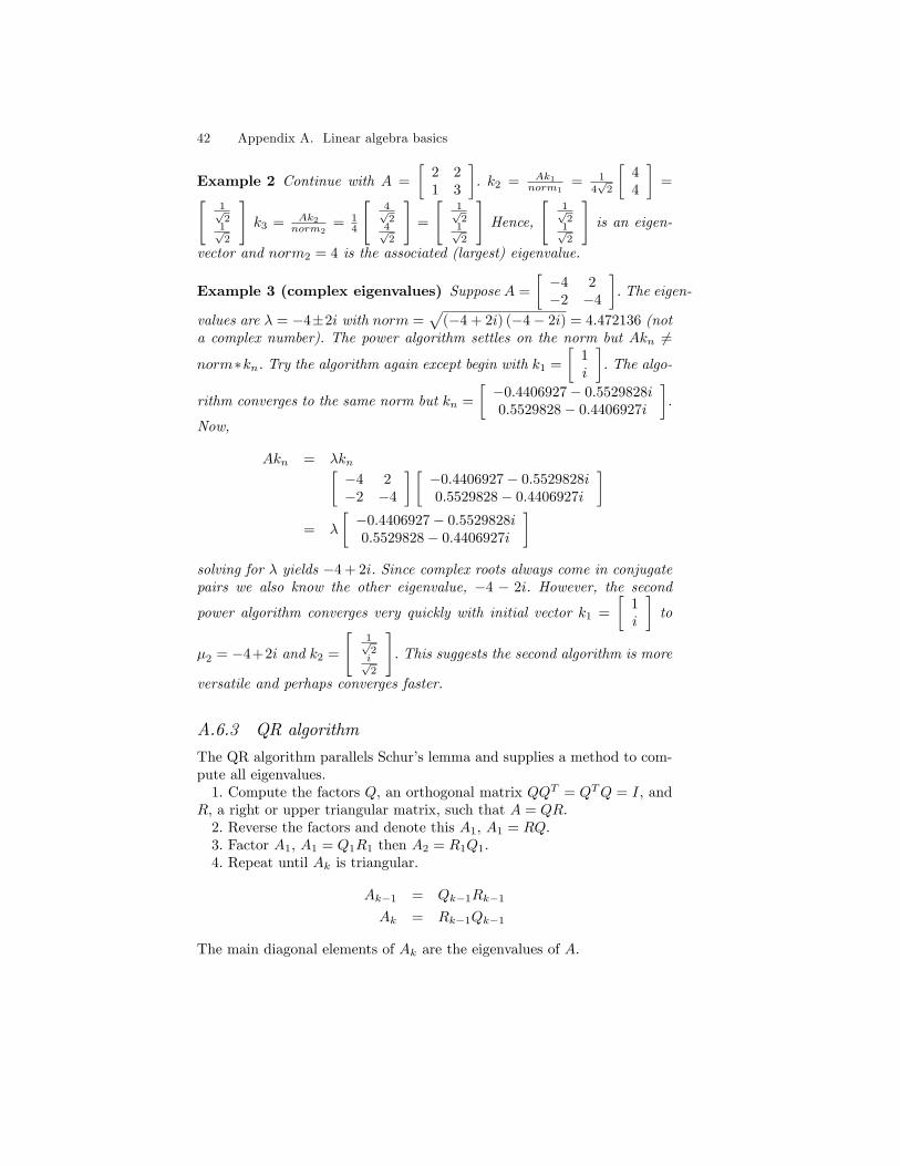
Example 2 Continue with A =
[2 21 3
]. k2 = Ak1
norm1= 1
4√
2
[44
]=[
1√2
1√2
]k3 = Ak2
norm2= 1
4
[4√2
4√2
]=
[1√2
1√2
]Hence,
[1√2
1√2
]is an eigen-
vector and norm2 = 4 is the associated (largest) eigenvalue.
Example 3 (complex eigenvalues) Suppose A =
[−4 2−2 −4
]. The eigen-
values are λ = −4±2i with norm =√
(−4 + 2i) (−4− 2i) = 4.472136 (nota complex number). The power algorithm settles on the norm but Akn 6=
norm∗kn. Try the algorithm again except begin with k1 =
[1i
]. The algo-
rithm converges to the same norm but kn =
[−0.4406927− 0.5529828i0.5529828− 0.4406927i
].
Now,
Akn = λkn[−4 2−2 −4
] [−0.4406927− 0.5529828i0.5529828− 0.4406927i
]= λ
[−0.4406927− 0.5529828i0.5529828− 0.4406927i
]solving for λ yields −4 + 2i. Since complex roots always come in conjugatepairs we also know the other eigenvalue, −4 − 2i. However, the second
power algorithm converges very quickly with initial vector k1 =
[1i
]to
µ2 = −4+2i and k2 =
[1√2i√2
]. This suggests the second algorithm is more
versatile and perhaps converges faster.
A.6.3 QR algorithm
The QR algorithm parallels Schur’s lemma and supplies a method to com-pute all eigenvalues.1. Compute the factors Q, an orthogonal matrix QQT = QTQ = I, and
R, a right or upper triangular matrix, such that A = QR.2. Reverse the factors and denote this A1, A1 = RQ.3. Factor A1, A1 = Q1R1 then A2 = R1Q1.4. Repeat until Ak is triangular.
Ak−1 = Qk−1Rk−1
Ak = Rk−1Qk−1
The main diagonal elements of Ak are the eigenvalues of A.
A.6 Computing eigenvalues 43
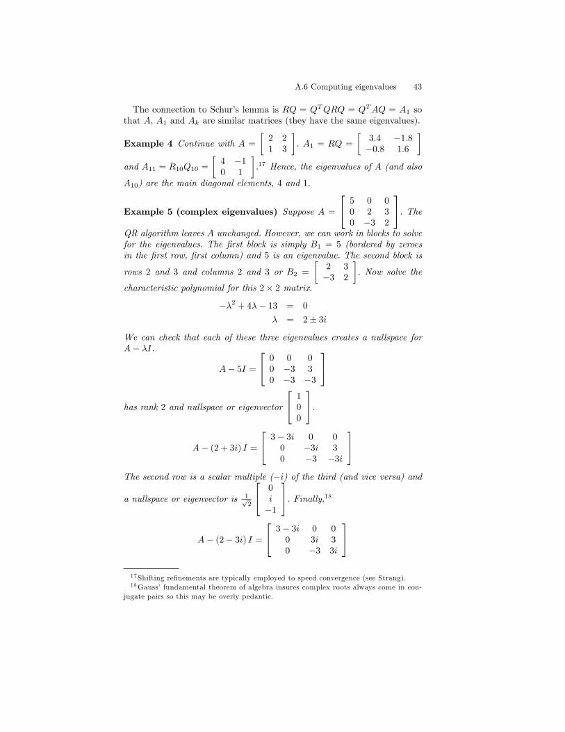
The connection to Schur’s lemma is RQ = QTQRQ = QTAQ = A1 sothat A, A1 and Ak are similar matrices (they have the same eigenvalues).
Example 4 Continue with A =
[2 21 3
]. A1 = RQ =
[3.4 −1.8−0.8 1.6
]and A11 = R10Q10 =
[4 −10 1
].17 Hence, the eigenvalues of A (and also
A10) are the main diagonal elements, 4 and 1.
Example 5 (complex eigenvalues) Suppose A =
5 0 00 2 30 −3 2
. TheQR algorithm leaves A unchanged. However, we can work in blocks to solvefor the eigenvalues. The first block is simply B1 = 5 (bordered by zeroesin the first row, first column) and 5 is an eigenvalue. The second block is
rows 2 and 3 and columns 2 and 3 or B2 =
[2 3−3 2
]. Now solve the
characteristic polynomial for this 2× 2 matrix.
−λ2 + 4λ− 13 = 0
λ = 2± 3i
We can check that each of these three eigenvalues creates a nullspace forA− λI.
A− 5I =
0 0 00 −3 30 −3 −3
has rank 2 and nullspace or eigenvector
100
.A− (2 + 3i) I =
3− 3i 0 00 −3i 30 −3 −3i
The second row is a scalar multiple (−i) of the third (and vice versa) and
a nullspace or eigenvector is 1√2
0i−1
. Finally,18
A− (2− 3i) I =
3− 3i 0 00 3i 30 −3 3i
17Shifting refinements are typically employed to speed convergence (see Strang).18Gauss’fundamental theorem of algebra insures complex roots always come in con-
jugate pairs so this may be overly pedantic.
44 Appendix A. Linear algebra basics
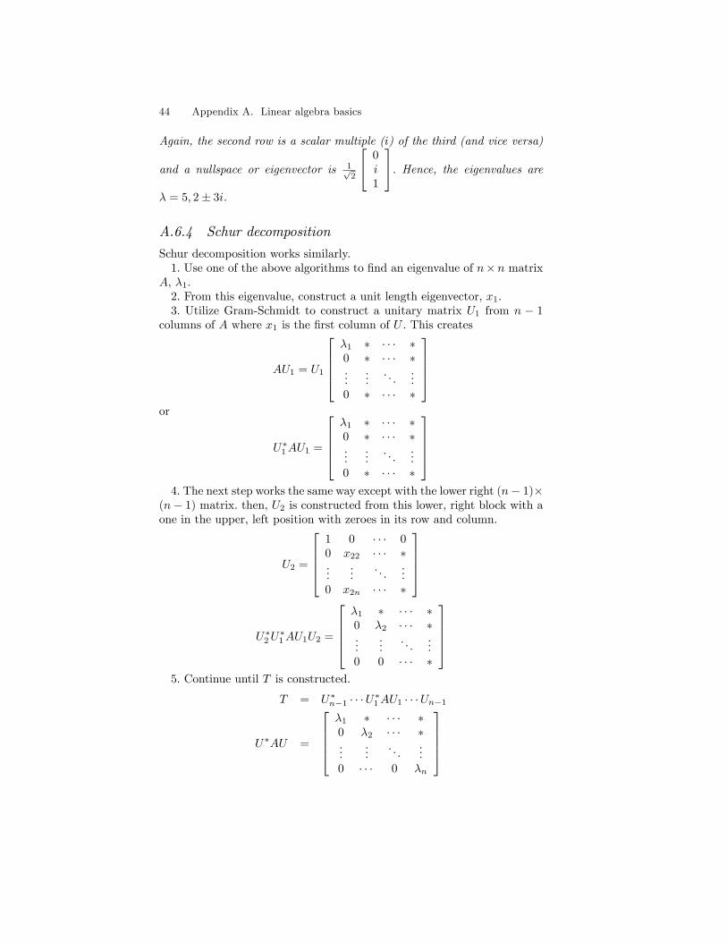
Again, the second row is a scalar multiple (i) of the third (and vice versa)
and a nullspace or eigenvector is 1√2
0i1
. Hence, the eigenvalues areλ = 5, 2± 3i.
A.6.4 Schur decomposition
Schur decomposition works similarly.1. Use one of the above algorithms to find an eigenvalue of n× n matrix
A, λ1.2. From this eigenvalue, construct a unit length eigenvector, x1.3. Utilize Gram-Schmidt to construct a unitary matrix U1 from n − 1
columns of A where x1 is the first column of U . This creates
AU1 = U1
λ1 ∗ · · · ∗0 ∗ · · · ∗...
.... . .
...0 ∗ · · · ∗
or
U∗1AU1 =
λ1 ∗ · · · ∗0 ∗ · · · ∗...
.... . .
...0 ∗ · · · ∗
4. The next step works the same way except with the lower right (n− 1)×
(n− 1) matrix. then, U2 is constructed from this lower, right block with aone in the upper, left position with zeroes in its row and column.
U2 =
1 0 · · · 00 x22 · · · ∗...
.... . .
...0 x2n · · · ∗
U∗2U∗1AU1U2 =
λ1 ∗ · · · ∗0 λ2 · · · ∗...
.... . .
...0 0 · · · ∗
5. Continue until T is constructed.
T = U∗n−1 · · ·U∗1AU1 · · ·Un−1
U∗AU =
λ1 ∗ · · · ∗0 λ2 · · · ∗...
.... . .
...0 · · · 0 λn
A.6 Computing eigenvalues 45
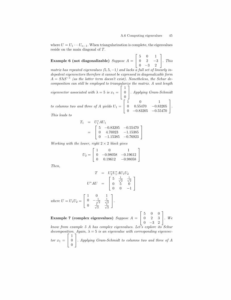
where U = U1 · · ·Un−1. When triangularization is complete, the eigenvaluesreside on the main diagonal of T .
Example 6 (not diagonalizable) Suppose A =
5 0 10 2 −30 −3 2
. Thismatrix has repeated eigenvalues (5, 5,−1) and lacks a full set of linearly in-depedent eigenvectors therefore it cannot be expressed in diagonalizable formA = SΛS−1 (as the latter term doesn’t exist). Nonetheless, the Schur de-composition can still be employed to triangularize the matrix. A unit length
eigenvector associated with λ = 5 is x1 =
100
. Applying Gram-Schmidtto columns two and three of A yields U1 =
1 0 10 0.55470 −0.832050 −0.83205 −0.55470
.This leads to
T1 = U∗1AU1
=
5 −0.83205 −0.554700 4.76923 −1.153850 −1.15385 −0.76923
Working with the lower, right 2× 2 block gives
U2 =
1 0 10 −0.98058 −0.196120 0.19612 −0.98058
Then,
T = U∗2U∗1AU1U2
U∗AU =
5 1√2
1√2
0 5 00 0 −1
where U = U1U2 =
1 0 10 − 1√
21√2
0 1√2
1√2
.Example 7 (complex eigenvalues) Suppose A =
5 0 00 2 30 −3 2
. Weknow from example 5 A has complex eigenvalues. Let’s explore its Schurdecomposition. Again, λ = 5 is an eigenvalue with corresponding eigenvec-
tor x1 =
100
. Applying Gram-Schmidt to columns two and three of A
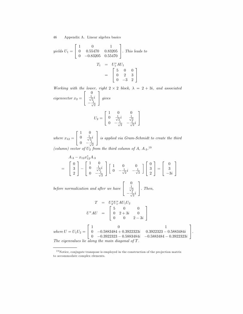
46 Appendix A. Linear algebra basics
yields U1 =
1 0 10 0.55470 0.832050 −0.83205 0.55470
. This leads toT1 = U∗1AU1
=
5 0 00 2 30 −3 2
Working with the lower, right 2 × 2 block, λ = 2 + 3i, and associated
eigenvector x2 =
01√2i
− 1√2
gives
U2 =
1 0 00 1√
2i 1√
2
0 − 1√2− 1√
2i
where x12 =
1 00 1√
2i
0 − 1√2
is applied via Gram-Schmidt to create the third(column) vector of U2 from the third column of A, A·3.19
A·3 − x12x∗12A·3
=
032
− 1 0
0 1√2i
0 − 1√2
[ 1 0 00 − 1√
2i − 1√
2
] 032
=
03−3i
before normalization and after we have
01√2
− 1√2i
. Then,T = U∗2U
∗1AU1U2
U∗AU =
5 0 00 2 + 3i 00 0 2− 3i
where U = U1U2 =
1 0 10 −0.5883484 + 0.3922323i 0.3922323− 0.5883484i0 −0.3922323− 0.5883484i −0.5883484− 0.3922323i
.The eigenvalues lie along the main diagonal of T .
19Notice, conjugate transpose is employed in the construction of the projection matrixto accommodate complex elements.
A.7 Some determinant identities 47
A.7 Some determinant identities
A.7.1 Determinant of a square matrix
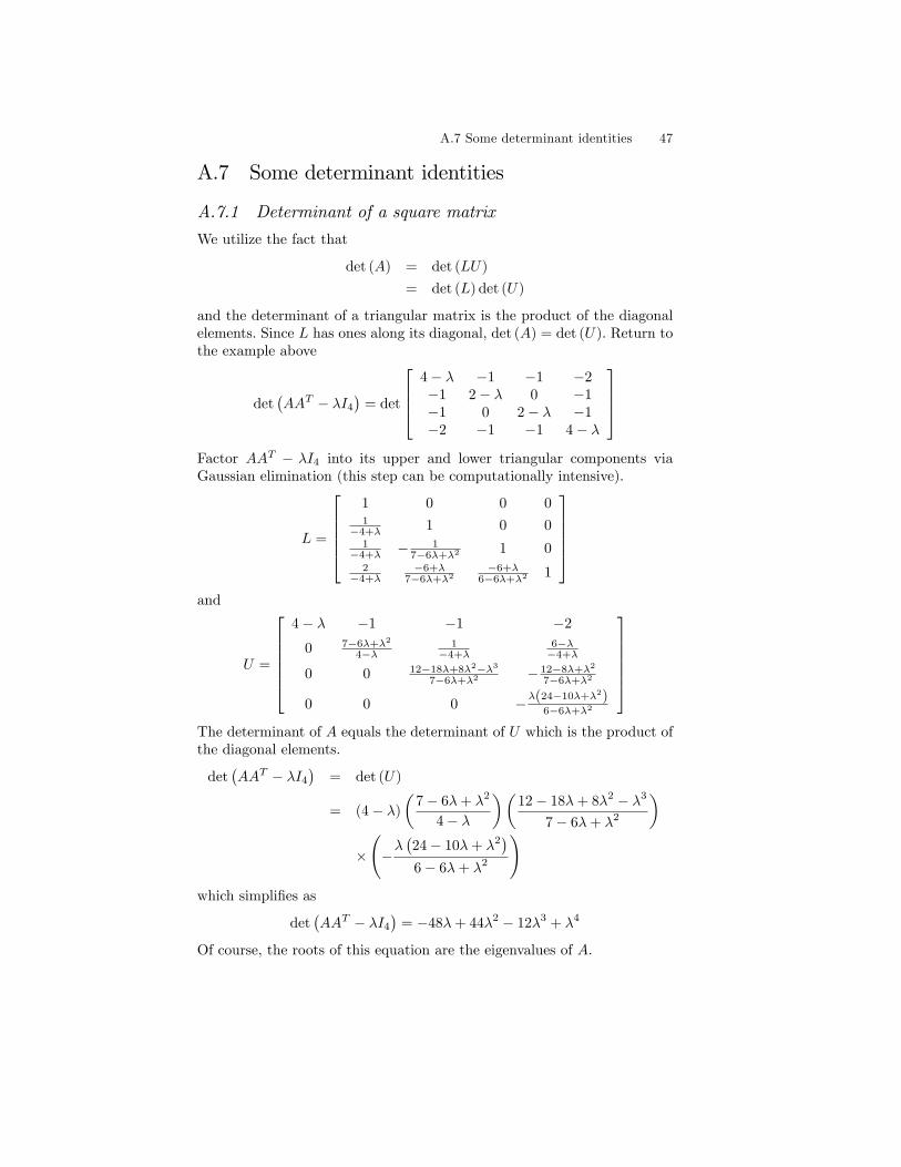
We utilize the fact that
det (A) = det (LU)
= det (L) det (U)
and the determinant of a triangular matrix is the product of the diagonalelements. Since L has ones along its diagonal, det (A) = det (U). Return tothe example above
det(AAT − λI4
)= det
4− λ −1 −1 −2−1 2− λ 0 −1−1 0 2− λ −1−2 −1 −1 4− λ
Factor AAT − λI4 into its upper and lower triangular components viaGaussian elimination (this step can be computationally intensive).
L =
1 0 0 01
−4+λ 1 0 01
−4+λ − 17−6λ+λ2
1 02
−4+λ−6+λ
7−6λ+λ2−6+λ
6−6λ+λ21
and
U =
4− λ −1 −1 −2
0 7−6λ+λ2
4−λ1
−4+λ6−λ−4+λ
0 0 12−18λ+8λ2−λ37−6λ+λ2
− 12−8λ+λ2
7−6λ+λ2
0 0 0 −λ(24−10λ+λ2)6−6λ+λ2
The determinant of A equals the determinant of U which is the product ofthe diagonal elements.
det(AAT − λI4
)= det (U)
= (4− λ)
(7− 6λ+ λ2
4− λ
)(12− 18λ+ 8λ2 − λ3
7− 6λ+ λ2
)×(−λ(24− 10λ+ λ2
)6− 6λ+ λ2
)which simplifies as
det(AAT − λI4
)= −48λ+ 44λ2 − 12λ3 + λ4
Of course, the roots of this equation are the eigenvalues of A.
48 Appendix A. Linear algebra basics
A.7.2 Identities
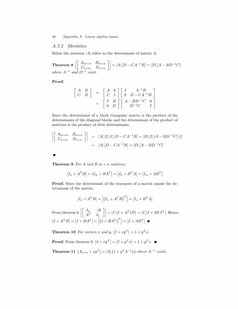
Below the notation |A| refers to the determinant of matrix A.
Theorem 8∣∣∣∣[ Am×m Bm×n
Cn×m Dn×n
]∣∣∣∣ = |A|∣∣D − CA−1B
∣∣ = |D|∣∣A−BD−1C
∣∣where A−1 and D−1 exist.
Proof. [A BC D
]=
[A 0C I
] [I A−1B0 D − CA−1B
]=
[I B0 D
] [A−BD−1C 0
D−1C I
]Since the determinant of a block triangular matrix is the product of thedeterminants of the diagonal blocks and the determinant of the product ofmatrices is the product of their determinants,∣∣∣∣[ Am×m Bm×n
Cn×m Dn×n
]∣∣∣∣ = |A| |I| |I|∣∣D − CA−1B
∣∣ = |D| |I|∣∣A−BD−1C
∣∣ |I|= |A|
∣∣D − CA−1B∣∣ = |D|
∣∣A−BD−1C∣∣
Theorem 9 For A and B m× n matrices,∣∣In +ATB∣∣ =
∣∣Im +BAT∣∣ =
∣∣In +BTA∣∣ =
∣∣Im +ABT∣∣
Proof. Since the determinant of the transpose of a matrix equals the de-terminant of the matrix,
∣∣In +ATB∣∣ =
∣∣∣(In +ATB)T ∣∣∣ =
∣∣In +BTA∣∣
From theorem 8,
∣∣∣∣[ Im −BAT In
]∣∣∣∣ = |I|∣∣I +AT IB
∣∣ = |I|∣∣I +BIAT
∣∣. Hence,∣∣I +ATB∣∣ =
∣∣I +BAT∣∣ =
∣∣∣(I +BAT)T ∣∣∣ =
∣∣I +ABT∣∣
Theorem 10 For vectors x and y,∣∣I + xyT
∣∣ = 1 + yTx.
Proof. From theorem 9,∣∣I + xyT
∣∣ =∣∣I + yTx
∣∣ = 1 + yTx.
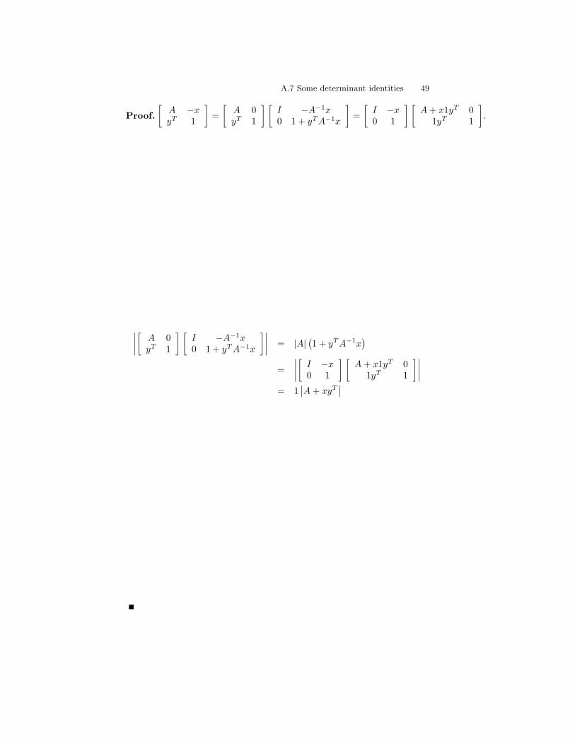
Theorem 11∣∣An×n + xyT
∣∣ = |A|(1 + yTA−1x
)where A−1 exists.
A.7 Some determinant identities 49
Proof.[A −xyT 1
]=
[A 0yT 1
] [I −A−1x0 1 + yTA−1x
]=
[I −x0 1
] [A+ x1yT 0
1yT 1
].
∣∣∣∣[ A 0yT 1
] [I −A−1x0 1 + yTA−1x
]∣∣∣∣ = |A|(1 + yTA−1x
)=
∣∣∣∣[ I −x0 1
] [A+ x1yT 0
1yT 1
]∣∣∣∣= 1
∣∣A+ xyT∣∣
50 Appendix A. Linear algebra basics
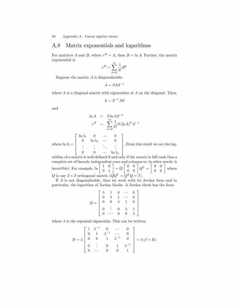
A.8 Matrix exponentials and logarithms
For matrices A and B, where eB = A, then B = lnA. Further, the matrixexponential is
eB =
∞∑k=0
1
k!Bk
Suppose the matrix A is diagonalizable.
A = SΛS−1
where Λ is a diagonal matrix with eigenvalues of A on the diagonal. Then,
Λ = S−1AS
and
lnA = S ln ΛS−1
eB =
∞∑k=0
1
k!S (ln Λ)
kS−1
where ln Λ =
lnλ1 0 · · · 0
0 lnλ2 · · · 0...
.... . .
...0 0 · · · lnλn
. From this result we see the log-arithm of a matrix is well-defined if and only if the matrix is full rank (has acomplete set of linearly independent rows and columns or, in other words, is
invertible). For example, ln
[1 00 1
]= Q
[0 00 0
]QT =
[0 00 0
]where
Q is any 2× 2 orthogonal matrix (QQT = QTQ = I).If A is not diagonalizable, then we work with its Jordan form and in
particular, the logarithm of Jordan blocks. A Jordan block has the form
B =
λ 1 0 · · · 00 λ 1 · · · 00 0 λ 1 0
0... 0 λ 1
0 · · · 0 0 λ
where λ is the repeated eigenvalue. This can be written
B = λ
1 λ−1 0 · · · 0
0 1 λ−1 · · · 0
0 0 1 λ−1 0
0... 0 1 λ−1
0 · · · 0 0 1
= λ (I +K)
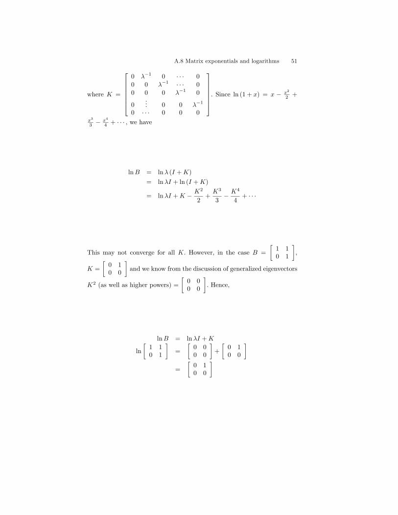
A.8 Matrix exponentials and logarithms 51
where K =
0 λ−1 0 · · · 0
0 0 λ−1 · · · 0
0 0 0 λ−1 0
0... 0 0 λ−1
0 · · · 0 0 0
. Since ln (1 + x) = x − x2
2 +
x3
3 −x4
4 + · · · , we have
lnB = lnλ (I +K)
= lnλI + ln (I +K)
= lnλI +K − K2
2+K3
3− K4
4+ · · ·
This may not converge for all K. However, in the case B =
[1 10 1
],
K =
[0 10 0
]and we know from the discussion of generalized eigenvectors
K2 (as well as higher powers) =
[0 00 0
]. Hence,
lnB = lnλI +K
ln
[1 10 1
]=
[0 00 0
]+
[0 10 0
]=
[0 10 0
]

52 Appendix A. Linear algebra basics
This is page 53Printer: Opaque this
Appendix BIterated expectations
Along with Bayes’ theorem (the glue holding consistent probability as-sessment together), iterated expectations is extensively employed for con-necting conditional expectation (regression) results with causal effects ofinterest.
Theorem 12 Law of iterated expectations
E [Y ] = EX [E [Y | X]]
Proof.
EX [E [Y | X]] =
∫ x
x
E [Y | X] f (x) dx
=
∫ x
x
[∫ y
y
yf (y | x) dy
]f (x) dx
By Fubini’s theorem, we can change the order of integration∫ x
x
[∫ y
y
yf (y | x) dy
]f (x) dx =
∫ y
y
y
[∫ x
x
f (y | x) f (x) dx
]dy
The product rule of Bayes’theorem, f (y | x) f (x) = f (y, x), implies iter-ated expectations can be rewritten as
EX [E [Y | X]] =
∫ y
y
y
[∫ x
x
f (y, x) dx
]dy

54 Appendix B. Iterated expectations
Finally, the summation rule integrates out X,∫ xxf (y, x) dx = f (y), and
produces the result.
EX [E [Y | X]] =
∫ y
y
yf (y) dy = E [Y ]
B.1 Decomposition of variance 55
B.1 Decomposition of variance
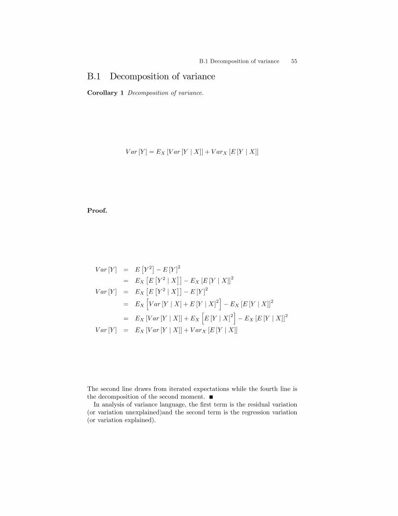
Corollary 1 Decomposition of variance.
V ar [Y ] = EX [V ar [Y | X]] + V arX [E [Y | X]]
Proof.
V ar [Y ] = E[Y 2]− E [Y ]
2
= EX[E[Y 2 | X
]]− EX [E [Y | X]]
2
V ar [Y ] = EX[E[Y 2 | X
]]− E [Y ]
2
= EX
[V ar [Y | X] + E [Y | X]
2]− EX [E [Y | X]]
2
= EX [V ar [Y | X]] + EX
[E [Y | X]
2]− EX [E [Y | X]]
2
V ar [Y ] = EX [V ar [Y | X]] + V arX [E [Y | X]]
The second line draws from iterated expectations while the fourth line isthe decomposition of the second moment.In analysis of variance language, the first term is the residual variation
(or variation unexplained)and the second term is the regression variation(or variation explained).
56 Appendix B. Iterated expectations
B.2 Jensen’s inequality
For any concave function g (x), E [g (x)] ≤ g (E [x]). Likewise, for any con-vex function h (x), E [h (x)] ≥ h (E [x]). Hence, utility functions exhibitingconcavity characterize risk aversion or positive risk premia while utilityfunctions exhibiting convexity characterize risk-seeking preferences or neg-ative risk premia.Further, Jensen’s inequality tells us the geometric mean, G (x), is less
than or equal to the arithmetic mean, A (x), with equality only when alloutcomes are the same.
G (x) ≡n∏i=1
xpii ≤ A (x) ≡n∑i=1
pixi
To see this result, let g (·) be the logarithm (a monotone increasing, concavefunction) for x nonnegative (if any xi = 0 then the inequality is triviallysatisfied as the geometric mean is zero if any xi = 0)
E [g (x)] =
n∑i=1
pi lnxi ≤ g (E [x]) = ln
n∑i=1
pixi
Let pi = wiw where w =
∑ni=1 wi, then
n∑i=1
wiw
lnxi ≤ ln
n∑i=1
wiwxi
To recover geometric and arithmetic means exponentiate (a monotone in-creasing function) both sides
w
√n∏i=1
xwii = G (x) ≤n∑i=1
wiwxi = A (x)
This is page 57Printer: Opaque this
Appendix CMultivariate normal theory
The Gaussian or normal probability distribution is ubiquitous when thedata have continuous support as seen in the Central Limit theorems andthe resilience to transformation of Gaussian random variables. When con-fronted with a vector of variables (multivariate), it often is sensible to thinkof a joint normal probability assignment to describe their stochastic prop-
erties. Let W =
[XZ
]be an m-element vector (X has m1 elements and
Z has m2 variables such that m1 +m2 = m) with joint normal probability,then the density function is
fW (w) =1
(2π)m/2 |Σ|1/2
exp
[−1
2(w − µ)
TΣ−1 (w − µ)
]where
µ =
[µXµZ
]is the m-element vector of means for W and
Σ =
[ΣXX ΣXZΣZX ΣZZ
]is them×m variance-covariance matrix forW withm linearly independentrows and columns.Of course, the density integrates to unity,
∫X
∫ZfW (w) dzdx = 1. And,
the marginal densities are found by integrating out the other variables, forexample, fX (x) =
∫ZfW (w) dz and fZ (z) =
∫XfW (w) dx.
58 Appendix C. Multivariate normal theory
Importantly, as it unifies linear regression, the conditional distributionsare also Gaussian.
fX (x | Z = z) =fW (w)
fZ (z)
∼ N (E [X | Z = z] , V ar [X | Z])
where
E [X | Z = z] = µX + ΣXZΣ−1ZZ (z − µZ)
and
V ar [X | Z] = ΣXX − ΣXZΣ−1ZZΣZX
Also,
fZ (z | X = x) ∼ N (E [Z | X = x] , V ar [Z | X])
where
E [Z | X = x] = µZ + ΣZXΣ−1XX (x− µX)
and
V ar [Z | X] = ΣZZ − ΣZXΣ−1XXΣXZ
From the conditional expectation (or regression) function we see when thedata are Gaussian, linearity imposes no restriction.
E [Z | X = x] = µZ + ΣZXΣ−1XX (x− µX)
is often written
E [Z | X = x] =(I − ΣZXΣ−1
XX
)µZ + ΣZXΣ−1
XXx
= α+ βTx
where α corresponds to an intercept (or vector of intercepts) and βTxcorresponds to weighted regressors. Applied linear regression estimates thesample analogs to the above parameters, α and β.
C.1 Conditional distribution 59
C.1 Conditional distribution
Next, we develop more carefully the result for fX (x | Z = z); the result forfZ (z | X = x) follows in analogous fashion.
fX (x | Z) =fW (w)
fZ (z)
=
1(2π)m/2|Σ|1/2 exp
[− 1
2 (w − µ)T
Σ−1 (w − µ)]
1(2π)m2/2|ΣZZ |1/2
exp[− 1
2 (z − µZ)T
Σ−1ZZ (z − µz)
]=
1
(2π)m1/2 |V ar [X | Z]|1/2
× exp
[−1
2(x− E [X | Z])
TV ar [X | Z]
−1(x− E [X | Z])
]The normalizing constants are identified almost immediately since
(2π)m/2
(2π)m2/2
=(2π)
(m1+m2)/2
(2π)m2/2
= (2π)m1/2
for the leading term and by theorem 1 in section A.6.2 we have
|Σ| = |ΣZZ |∣∣ΣXX − ΣXZΣ−1
ZZΣZX∣∣
since ΣXX , ΣZZ , and Σ are positive definite, their determinants are positiveand their square roots are real. Hence,
|Σ|12
|ΣZZ |12
=|ΣZZ |
12∣∣ΣXX − ΣXZΣ−1
ZZΣZX∣∣ 12
|ΣZZ |12
=∣∣ΣXX − ΣXZΣ−1
ZZΣZX∣∣ 12
= |V ar [X | Z]|12
This leaves the exponential terms
exp[− 1
2 (w − µ)T
Σ−1 (w − µ)]
exp[− 1
2 (z − µZ)T
Σ−1ZZ (z − µz)
]= exp
[−1
2(w − µ)
TΣ−1 (w − µ) +
1
2(z − µZ)
TΣ−1ZZ (z − µz)
]which require a bit more foundation. We begin with a lemma for the inverseof a partitioned matrix.
60 Appendix C. Multivariate normal theory
Lemma 1 Let a symmetric, positive definite matrix H be partitioned as[A BT
B C
]where A and C are square n1×n1 and n2×n2 positive definite
matrices (their inverses exist). Then,
H−1 =
[ (A−BTC−1B
)−1 −A−1BT(C −BA−1BT
)−1
−C−1B(A−BTC−1B
)−1 (C −BA−1BT
)−1
]
=
[ (A−BTC−1B
)−1 −(A−BTC−1B
)−1BTC−1
−C−1B(A−BTC−1B
)−1 (C −BA−1BT
)−1
]
=
[ (A−BTC−1B
)−1 −A−1BT(C −BA−1BT
)−1
−(C −BA−1BT
)−1BA−1
(C −BA−1BT
)−1
]Proof. H is symmetric and the inverse of a symmetric matrix is also sym-metric. Hence, the second and third lines follow from symmetry and thefirst line. Since H is symmetric, positive definite,
H = LDLT
=
[I 0
BA−1 I
] [A 00 C −BA−1BT
] [I A−1BT
0 I
]and
H−1 =(LT)−1
D−1L−1
=
[I −A−1BT
0 I
] [A−1 0
0(C −BA−1BT
)−1
] [I 0
−BA−1 I
]Expanding gives
H−1 =
[X −A−1BT
(C −BA−1BT
)−1
−(C −BA−1BT
)−1BA−1
(C −BA−1BT
)−1
]where
X = A−1 +A−1BT(C −BA−1BT
)−1BA−1 =
(A−BTC−1B
)−1
The latter equality follows from some linear algebra. Suppose it’s true(A−BTC−1B
)−1= A−1 +A−1BT
(C −BA−1BT
)−1BA−1
pre- and post-multiply both sides by A
A(A−BTC−1B
)−1A = A+BT
(C −BA−1BT
)−1B
post multiply both sides by A−1(A−BTC−1B
)A =
(A−BTC−1B
)+BT
(C −BA−1BT
)−1BA−1
(A−BTC−1B
)0 = −BTC−1B +BT
(C −BA−1BT
)−1BA−1
(A−BTC−1B
)
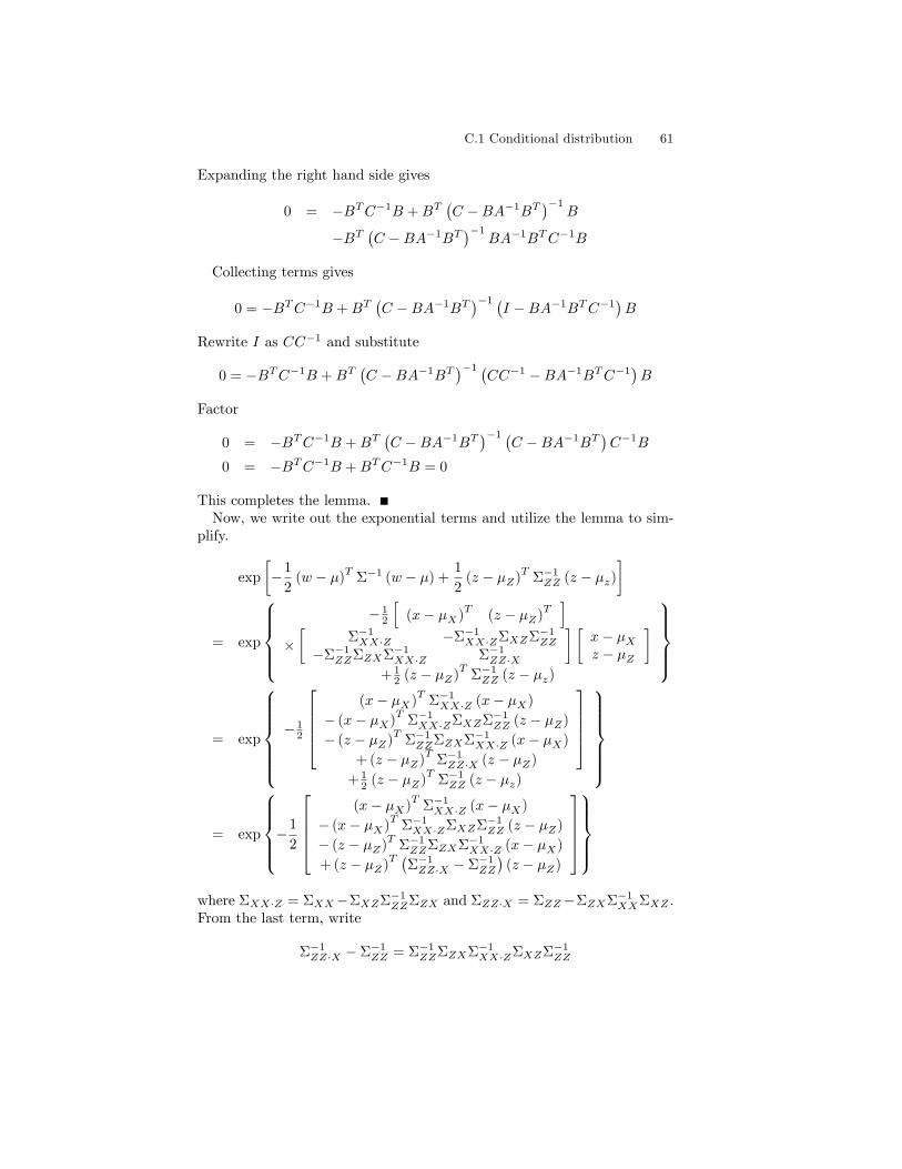
C.1 Conditional distribution 61
Expanding the right hand side gives
0 = −BTC−1B +BT(C −BA−1BT
)−1B
−BT(C −BA−1BT
)−1BA−1BTC−1B
Collecting terms gives
0 = −BTC−1B +BT(C −BA−1BT
)−1 (I −BA−1BTC−1
)B
Rewrite I as CC−1 and substitute
0 = −BTC−1B +BT(C −BA−1BT
)−1 (CC−1 −BA−1BTC−1
)B
Factor
0 = −BTC−1B +BT(C −BA−1BT
)−1 (C −BA−1BT
)C−1B
0 = −BTC−1B +BTC−1B = 0
This completes the lemma.Now, we write out the exponential terms and utilize the lemma to sim-
plify.
exp
[−1
2(w − µ)
TΣ−1 (w − µ) +
1
2(z − µZ)
TΣ−1ZZ (z − µz)
]
= exp
− 1
2
[(x− µX)
T(z − µZ)
T]
×[
Σ−1XX·Z −Σ−1
XX·ZΣXZΣ−1ZZ
−Σ−1ZZΣZXΣ−1
XX·Z Σ−1ZZ·X
] [x− µXz − µZ
]+ 1
2 (z − µZ)T
Σ−1ZZ (z − µz)
= exp
− 1
2
(x− µX)
TΣ−1XX·Z (x− µX)
− (x− µX)T
Σ−1XX·ZΣXZΣ−1
ZZ (z − µZ)
− (z − µZ)T
Σ−1ZZΣZXΣ−1
XX·Z (x− µX)
+ (z − µZ)T
Σ−1ZZ·X (z − µZ)
+ 1
2 (z − µZ)T
Σ−1ZZ (z − µz)
= exp
−1
2
(x− µX)
TΣ−1XX·Z (x− µX)
− (x− µX)T
Σ−1XX·ZΣXZΣ−1
ZZ (z − µZ)
− (z − µZ)T
Σ−1ZZΣZXΣ−1
XX·Z (x− µX)
+ (z − µZ)T (
Σ−1ZZ·X − Σ−1
ZZ
)(z − µZ)
where ΣXX·Z = ΣXX−ΣXZΣ−1ZZΣZX and ΣZZ·X = ΣZZ−ΣZXΣ−1
XXΣXZ .From the last term, write
Σ−1ZZ·X − Σ−1
ZZ = Σ−1ZZΣZXΣ−1
XX·ZΣXZΣ−1ZZ
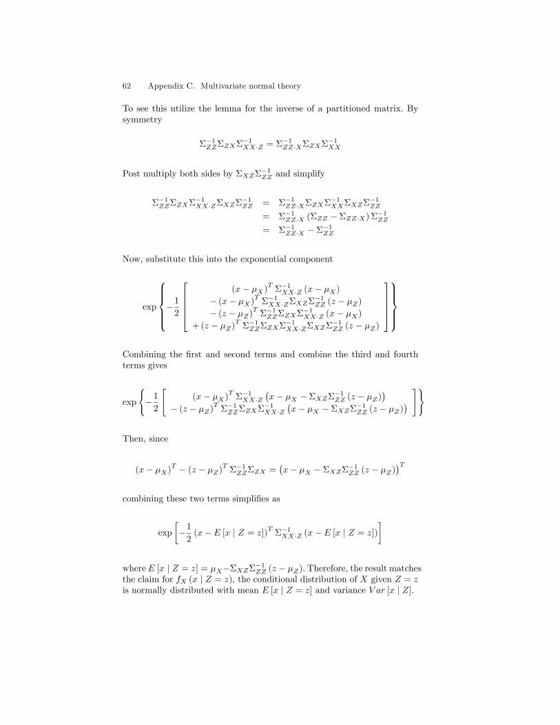
62 Appendix C. Multivariate normal theory
To see this utilize the lemma for the inverse of a partitioned matrix. Bysymmetry
Σ−1ZZΣZXΣ−1
XX·Z = Σ−1ZZ·XΣZXΣ−1
XX
Post multiply both sides by ΣXZΣ−1ZZ and simplify
Σ−1ZZΣZXΣ−1
XX·ZΣXZΣ−1ZZ = Σ−1
ZZ·XΣZXΣ−1XXΣXZΣ−1
ZZ
= Σ−1ZZ·X (ΣZZ − ΣZZ·X) Σ−1
ZZ
= Σ−1ZZ·X − Σ−1
ZZ
Now, substitute this into the exponential component
exp
−1
2
(x− µX)
TΣ−1XX·Z (x− µX)
− (x− µX)T
Σ−1XX·ZΣXZΣ−1
ZZ (z − µZ)
− (z − µZ)T
Σ−1ZZΣZXΣ−1
XX·Z (x− µX)
+ (z − µZ)T
Σ−1ZZΣZXΣ−1
XX·ZΣXZΣ−1ZZ (z − µZ)
Combining the first and second terms and combine the third and fourthterms gives
exp
{−1
2
[(x− µX)
TΣ−1XX·Z
(x− µX − ΣXZΣ−1
ZZ (z − µZ))
− (z − µZ)T
Σ−1ZZΣZXΣ−1
XX·Z(x− µX − ΣXZΣ−1
ZZ (z − µZ)) ]}
Then, since
(x− µX)T − (z − µZ)
TΣ−1ZZΣZX =
(x− µX − ΣXZΣ−1
ZZ (z − µZ))T
combining these two terms simplifies as
exp
[−1
2(x− E [x | Z = z])
TΣ−1XX·Z (x− E [x | Z = z])
]
where E [x | Z = z] = µX−ΣXZΣ−1ZZ (z − µZ). Therefore, the result matches
the claim for fX (x | Z = z), the conditional distribution of X given Z = zis normally distributed with mean E [x | Z = z] and variance V ar [x | Z].
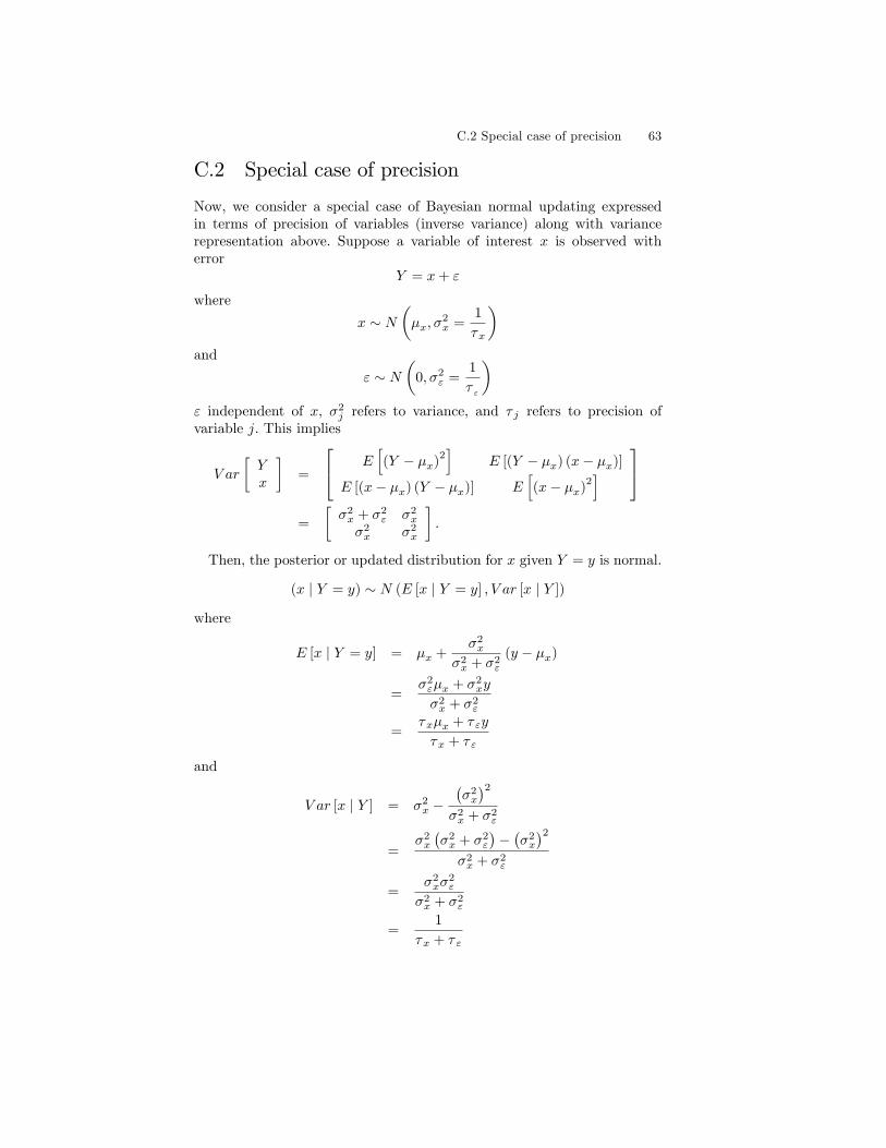
C.2 Special case of precision 63
C.2 Special case of precision
Now, we consider a special case of Bayesian normal updating expressedin terms of precision of variables (inverse variance) along with variancerepresentation above. Suppose a variable of interest x is observed witherror
Y = x+ ε
where
x ∼ N(µx, σ
2x =
1
τx
)and
ε ∼ N(
0, σ2ε =
1
τ ε
)ε independent of x, σ2
j refers to variance, and τ j refers to precision ofvariable j. This implies
V ar
[Yx
]=
E[(Y − µx)
2]
E [(Y − µx) (x− µx)]
E [(x− µx) (Y − µx)] E[(x− µx)
2]
=
[σ2x + σ2
ε σ2x
σ2x σ2
x
].
Then, the posterior or updated distribution for x given Y = y is normal.
(x | Y = y) ∼ N (E [x | Y = y] , V ar [x | Y ])
where
E [x | Y = y] = µx +σ2x
σ2x + σ2
ε
(y − µx)
=σ2εµx + σ2
xy
σ2x + σ2
ε
=τxµx + τεy
τx + τε
and
V ar [x | Y ] = σ2x −
(σ2x
)2σ2x + σ2
ε
=σ2x
(σ2x + σ2
ε
)−(σ2x
)2σ2x + σ2
ε
=σ2xσ
2ε
σ2x + σ2
ε
=1
τx + τε

64 Appendix C. Multivariate normal theory
For both the conditional expectation and variance, the penultimate lineexpresses the quantity in terms of variance and the last line expresses thesame quantity in terms of precision. The precision of x given Y is τx|Y =τx + τε.
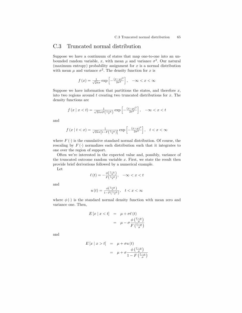
C.3 Truncated normal distribution 65
C.3 Truncated normal distribution
Suppose we have a continuum of states that map one-to-one into an un-bounded random variable, x, with mean µ and variance σ2. Our natural(maximum entropy) probability assignment for x is a normal distributionwith mean µ and variance σ2. The density function for x is
f (x) = 1√2πσ
exp[− (x−µ)2
2σ2
], −∞ < x <∞
Suppose we have information that partitions the states, and therefore x,into two regions around t creating two truncated distributions for x. Thedensity functions are
f (x | x < t) = 1√2πσF( t−µσ )
exp[− (x−µ)2
2σ2
], −∞ < x < t
and
f (x | t < x) = 1√2πσ[1−F( t−µσ )]
exp[− (x−µ)2
2σ2
], t < x <∞
where F (·) is the cumulative standard normal distribution. Of course, therescaling by F (·) normalizes each distribution such that it integrates toone over the region of support.Often we’re interested in the expected value and, possibly, variance of
the truncated outcome random variable x. First, we state the result thenprovide brief derivations followed by a numerical example.Let
` (t) = − φ( t−µσ )F( t−µσ )
, −∞ < x < t
and
u (t) =φ( t−µσ )
1−F( t−µσ ), t < x <∞
where φ (·) is the standard normal density function with mean zero andvariance one. Then,
E [x | x < t] = µ+ σ` (t)
= µ− σφ(t−µσ
)F(t−µσ
)and
E [x | x > t] = µ+ σu (t)
= µ+ σφ(t−µσ
)1− F
(t−µσ
)
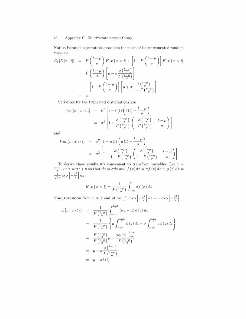
66 Appendix C. Multivariate normal theory
Notice, iterated expectations produces the mean of the untruncated randomvariable.
Et [E [x | t]] = F
(t− µσ
)E [x | x < t] +
[1− F
(t− µσ
)]E [x | x > t]
= F
(t− µσ
)[µ− σ
φ(t−µσ
)F(t−µσ
)]
+
[1− F
(t− µσ
)][µ+ σ
φ(t−µσ
)1− F
(t−µσ
)]= µ
Variances for the truncated distributions are
V ar [x | x < t] = σ2
[1− ` (t)
(` (t)− t− µ
σ
)]= σ2
[1 +
φ(t−µσ
)F(t−µσ
) (− φ ( t−µσ )F(t−µσ
) − t− µσ
)]and
V ar [x | x > t] = σ2
[1− u (t)
(u (t)− t− µ
σ
)]= σ2
[1−
φ(t−µσ
)1− F
(t−µσ
) ( φ(t−µσ
)1− F
(t−µσ
) − t− µσ
)]To derive these results it’s convenient to transform variables. Let z =
x−µσ , or x = σz+µ so that dx = σdz and f (x) dx = σf (z) dz ≡ φ (z) dz =1√2π
exp[− z22
]dz.
E [x | x < t] =1
F(t−µσ
) ∫ t
−∞xf (x) dx
Now, transform from x to z and utilize∫z exp
[− z22
]dz = − exp
[− z22
].
E [x | x < t] =1
F(t−µσ
) ∫ t−µσ
−∞(σz + µ)φ (z) dz
=1
F(t−µσ
) {µ∫ t−µσ
−∞φ (z) dz + σ
∫ t−µσ
−∞zφ (z) dz
}
=F(t−µσ
)F(t−µσ
)µ− σφ (z) |t−µσ−∞
F(t−µσ
)= µ− σ
φ(t−µσ
)F(t−µσ
)= µ− σ` (t)
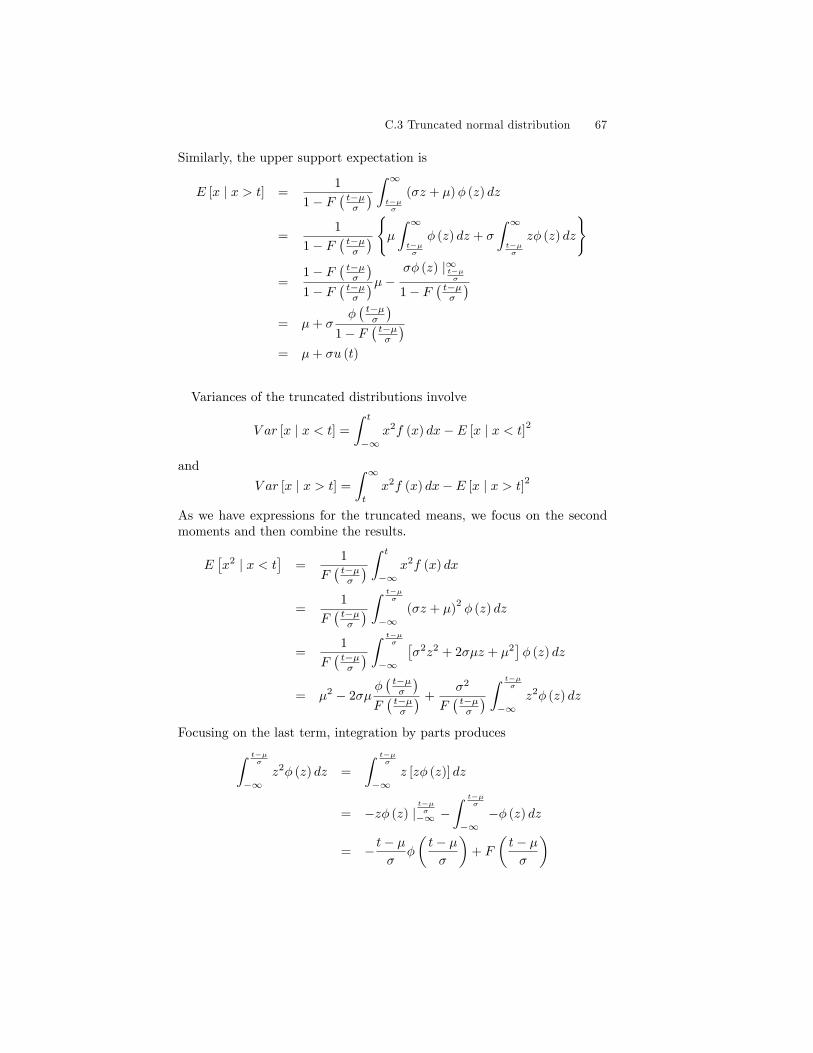
C.3 Truncated normal distribution 67
Similarly, the upper support expectation is
E [x | x > t] =1
1− F(t−µσ
) ∫ ∞t−µσ
(σz + µ)φ (z) dz
=1
1− F(t−µσ
) {µ∫ ∞t−µσ
φ (z) dz + σ
∫ ∞t−µσ
zφ (z) dz
}
=1− F
(t−µσ
)1− F
(t−µσ
)µ− σφ (z) |∞t−µσ
1− F(t−µσ
)= µ+ σ
φ(t−µσ
)1− F
(t−µσ
)= µ+ σu (t)
Variances of the truncated distributions involve
V ar [x | x < t] =
∫ t
−∞x2f (x) dx− E [x | x < t]
2
and
V ar [x | x > t] =
∫ ∞t
x2f (x) dx− E [x | x > t]2
As we have expressions for the truncated means, we focus on the secondmoments and then combine the results.
E[x2 | x < t
]=
1
F(t−µσ
) ∫ t
−∞x2f (x) dx
=1
F(t−µσ
) ∫ t−µσ
−∞(σz + µ)
2φ (z) dz
=1
F(t−µσ
) ∫ t−µσ
−∞
[σ2z2 + 2σµz + µ2
]φ (z) dz
= µ2 − 2σµφ(t−µσ
)F(t−µσ
) +σ2
F(t−µσ
) ∫ t−µσ
−∞z2φ (z) dz
Focusing on the last term, integration by parts produces∫ t−µσ
−∞z2φ (z) dz =
∫ t−µσ
−∞z [zφ (z)] dz
= −zφ (z) |t−µσ−∞ −
∫ t−µσ
−∞−φ (z) dz
= − t− µσ
φ
(t− µσ
)+ F
(t− µσ
)
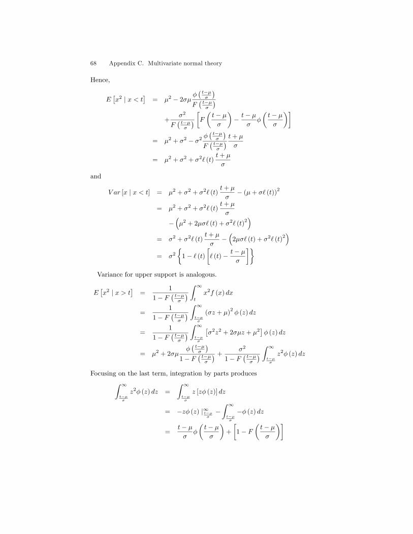
68 Appendix C. Multivariate normal theory
Hence,
E[x2 | x < t
]= µ2 − 2σµ
φ(t−µσ
)F(t−µσ
)+
σ2
F(t−µσ
) [F ( t− µσ
)− t− µ
σφ
(t− µσ
)]= µ2 + σ2 − σ2 φ
(t−µσ
)F(t−µσ
) t+ µ
σ
= µ2 + σ2 + σ2` (t)t+ µ
σ
and
V ar [x | x < t] = µ2 + σ2 + σ2` (t)t+ µ
σ− (µ+ σ` (t))
2
= µ2 + σ2 + σ2` (t)t+ µ
σ
−(µ2 + 2µσ` (t) + σ2` (t)
2)
= σ2 + σ2` (t)t+ µ
σ−(
2µσ` (t) + σ2` (t)2)
= σ2
{1− ` (t)
[` (t)− t− µ
σ
]}Variance for upper support is analogous.
E[x2 | x > t
]=
1
1− F(t−µσ
) ∫ ∞t
x2f (x) dx
=1
1− F(t−µσ
) ∫ ∞t−µσ
(σz + µ)2φ (z) dz
=1
1− F(t−µσ
) ∫ ∞t−µσ
[σ2z2 + 2σµz + µ2
]φ (z) dz
= µ2 + 2σµφ(t−µσ
)1− F
(t−µσ
) +σ2
1− F(t−µσ
) ∫ ∞t−µσ
z2φ (z) dz
Focusing on the last term, integration by parts produces∫ ∞t−µσ
z2φ (z) dz =
∫ ∞t−µσ
z [zφ (z)] dz
= −zφ (z) |∞t−µσ
−∫ ∞t−µσ
−φ (z) dz
=t− µσ
φ
(t− µσ
)+
[1− F
(t− µσ
)]
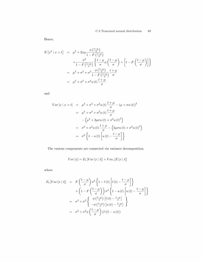
C.3 Truncated normal distribution 69
Hence,
E[x2 | x > t
]= µ2 + 2σµ
φ(t−µσ
)1− F
(t−µσ
)+
σ2
1− F(t−µσ
) { t− µσ
φ
(t− µσ
)+
[1− F
(t− µσ
)]}= µ2 + σ2 + σ2 φ
(t−µσ
)1− F
(t−µσ
) t+ µ
σ
= µ2 + σ2 + σ2u (t)t+ µ
σ
and
V ar [x | x > t] = µ2 + σ2 + σ2u (t)t+ µ
σ− (µ+ σu (t))
2
= µ2 + σ2 + σ2u (t)t+ µ
σ
−(µ2 + 2µσu (t) + σ2u (t)
2)
= σ2 + σ2u (t)t+ µ
σ−(
2µσu (t) + σ2u (t)2)
= σ2
{1− u (t)
[u (t)− t− µ
σ
]}
The various components are connected via variance decomposition.
V ar [x] = Et [V ar [x | t]] + V art [E [x | t]]
where
Et [V ar [x | t]] = F
(t− µσ
)σ2
{1− ` (t)
[` (t)− t− µ
σ
]}+
(1− F
(t− µσ
))σ2
{1− u (t)
[u (t)− t− µ
σ
]}= σ2 + σ2
{φ(t−µσ
) [` (t)− t−µ
σ
]−φ(t−µσ
) [u (t)− t−µ
σ
] }
= σ2 + σ2φ
(t− µσ
)(` (t)− u (t))
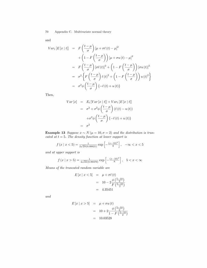
70 Appendix C. Multivariate normal theory
and
V art [E [x | t]] = F
(t− µσ
)[µ+ σ` (t)− µ]
2
+
(1− F
(t− µσ
))[µ+ σu (t)− µ]
2
= F
(t− µσ
)[σ` (t)]
2+
(1− F
(t− µσ
))[σu (t)]
2
= σ2
{F
(t− µσ
)` (t)
2+
(1− F
(t− µσ
))u (t)
2
}= σ2φ
(t− µσ
){−` (t) + u (t)}
Then,
V ar [x] = Et [V ar [x | t]] + V art [E [x | t]]
= σ2 + σ2φ
(t− µσ
)(` (t)− u (t))
+σ2φ
(t− µσ
){−` (t) + u (t)}
= σ2
Example 13 Suppose x ∼ N (µ = 10, σ = 2) and the distribution is trun-cated at t = 5. The density function at lower support is
f (x | x < 5) = 12√
2π(0.00621)exp
[− (x−10)2
8
], −∞ < x < 5
and at upper support is
f (x | x > 5) = 12√
2π(0.99379)exp
[− (x−10)2
8
], 5 < x <∞
Means of the truncated random variable are
E [x | x < 5] = µ+ σ` (t)
= 10− 2φ(
5−102
)F(
5−102
)= 4.35451
and
E [x | x > 5] = µ+ σu (t)
= 10 + 2φ(
5−102
)1− F
(5−10
2
)= 10.03528
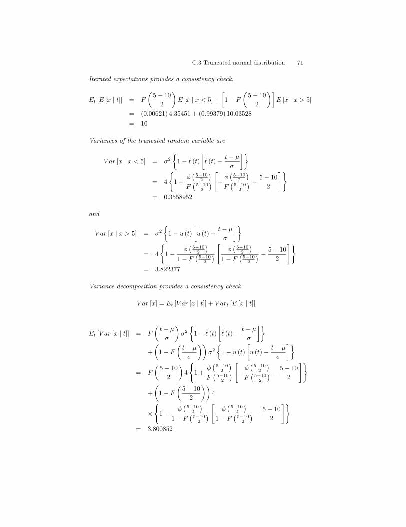
C.3 Truncated normal distribution 71
Iterated expectations provides a consistency check.
Et [E [x | t]] = F
(5− 10
2
)E [x | x < 5] +
[1− F
(5− 10
2
)]E [x | x > 5]
= (0.00621) 4.35451 + (0.99379) 10.03528
= 10
Variances of the truncated random variable are
V ar [x | x < 5] = σ2
{1− ` (t)
[` (t)− t− µ
σ
]}= 4
{1 +
φ(
5−102
)F(
5−102
) [− φ ( 5−102
)F(
5−102
) − 5− 10
2
]}= 0.3558952
and
V ar [x | x > 5] = σ2
{1− u (t)
[u (t)− t− µ
σ
]}= 4
{1−
φ(
5−102
)1− F
(5−10
2
) [ φ(
5−102
)1− F
(5−10
2
) − 5− 10
2
]}= 3.822377
Variance decomposition provides a consistency check.
V ar [x] = Et [V ar [x | t]] + V art [E [x | t]]
Et [V ar [x | t]] = F
(t− µσ
)σ2
{1− ` (t)
[` (t)− t− µ
σ
]}+
(1− F
(t− µσ
))σ2
{1− u (t)
[u (t)− t− µ
σ
]}= F
(5− 10
2
)4
{1 +
φ(
5−102
)F(
5−102
) [− φ ( 5−102
)F(
5−102
) − 5− 10
2
]}
+
(1− F
(5− 10
2
))4
×{
1−φ(
5−102
)1− F
(5−10
2
) [ φ(
5−102
)1− F
(5−10
2
) − 5− 10
2
]}= 3.800852
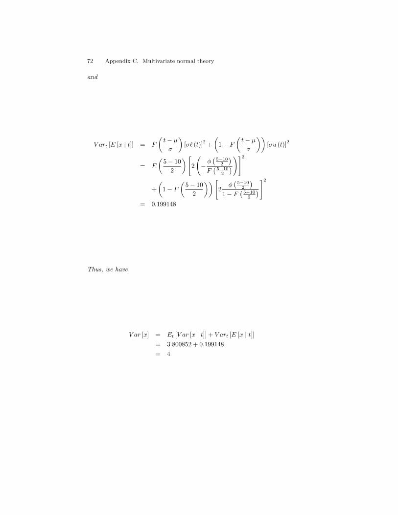
72 Appendix C. Multivariate normal theory
and
V art [E [x | t]] = F
(t− µσ
)[σ` (t)]
2+
(1− F
(t− µσ
))[σu (t)]
2
= F
(5− 10
2
)[2
(−φ(
5−102
)F(
5−102
))]2
+
(1− F
(5− 10
2
))[2
φ(
5−102
)1− F
(5−10
2
)]2
= 0.199148
Thus, we have
V ar [x] = Et [V ar [x | t]] + V art [E [x | t]]= 3.800852 + 0.199148
= 4
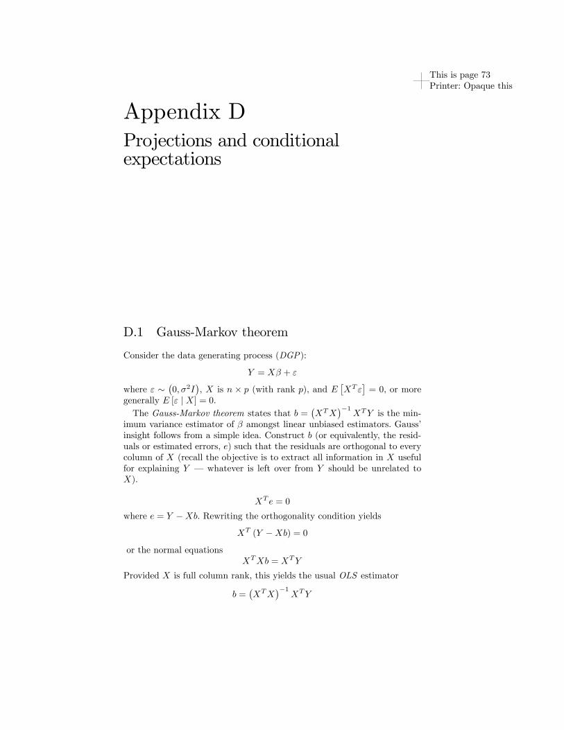
This is page 73Printer: Opaque this
Appendix DProjections and conditionalexpectations
D.1 Gauss-Markov theorem
Consider the data generating process (DGP):
Y = Xβ + ε
where ε ∼(0, σ2I
), X is n × p (with rank p), and E
[XT ε
]= 0, or more
generally E [ε | X] = 0.The Gauss-Markov theorem states that b =
(XTX
)−1XTY is the min-
imum variance estimator of β amongst linear unbiased estimators. Gauss’insight follows from a simple idea. Construct b (or equivalently, the resid-uals or estimated errors, e) such that the residuals are orthogonal to everycolumn of X (recall the objective is to extract all information in X usefulfor explaining Y – whatever is left over from Y should be unrelated toX).
XT e = 0
where e = Y −Xb. Rewriting the orthogonality condition yields
XT (Y −Xb) = 0
or the normal equationsXTXb = XTY
Provided X is full column rank, this yields the usual OLS estimator
b =(XTX
)−1XTY
74 Appendix D. Projections and conditional expectations
It is straightforward to show that b is unbiased (conditional on the dataX).
E [b | X] = E[(XTX
)−1XTY | X
]= E
[(XTX
)−1XT (Xβ + ε) | X
]= β +
(XTX
)−1XTE [ε | X] = β + 0 = β
Iterated expectations yields E [b] = EX [E [b | X]] = EX [β] = β. Hence,unbiasedness applies unconditionally as well.
V ar [b | X] = V ar[(XTX
)−1XTY | X
]= V ar
[(XTX
)−1XT (Xβ + ε) | X
]= E
[{β +
(XTX
)−1XT ε− β
}{(XTX
)−1XT ε
}T| X]
=(XTX
)−1XTE
[εεT]X(XTX
)−1
= σ2(XTX
)−1XT IX
(XTX
)−1
= σ2(XTX
)−1
Now, consider the stochastic regressors case,
V ar [b] = V arX [E [b | X]] + EX [V ar [b | X]]
The first term is zero since E [b | X] = β for all X. Hence,
V ar [b] = EX [V ar [b | X]] = σ2E[(XTX
)−1]
the unconditional variance of b can only be described in terms of the averagebehavior of X.To show that OLS yields the minimum variance linear unbiased esti-
mator consider another linear unbiased estimator b0 = LY (L replaces(XTX
)−1XT ). Since E [LY ] = E [LXβ + Lε] = β, LX = I.
Let D = L−(XTX
)−1XT so that DY = b0 − b.
V ar [b0 | X] = σ2[D +
(XTX
)−1XT] [D +
(XTX
)−1XT]T
= σ2
(DDT +
(XTX
)−1XTDT +DX
(XTX
)−1
+(XTX
)−1XTX
(XTX
)−1
)
SinceLX = I = DX +
(XTX
)−1XTX,DX = 0
D.1 Gauss-Markov theorem 75
and
V ar [b0 | X] = σ2(DDT +
(XTX
)−1)
As DDT is positive semidefinite, V ar [b] (and V ar [b | X]) is at least assmall as any other V ar [b0] (V ar [b0 | X]). Hence, the Gauss-Markov theo-rem applies to both nonstochastic and stochastic regressors.
Theorem 14 Rao-Blackwell theorem. If ε ∼ N(0, σ2I
)for the above DGP,
b has minimum variance of all unbiased estimators.
Finite sample inferences typically derive from normally distributed errorsand t (individual parameters) and F (joint parameters) statistics. Someasymptotic results related to the Rao-Blackwell theorem are as follows.For the Rao-Blackwell DGP , OLS is consistent and asymptotic normally(CAN ) distributed. Since MLE yields b for the above DGP with normallydistributed errors, OLS is asymptotically effi cient amongst all CAN esti-mators. Asymptotic inferences allow relaxation of the error distribution andrely on variations of the laws of large numbers and central limit theorems.
76 Appendix D. Projections and conditional expectations
D.2 Generalized least squares (GLS)
For the DGP,Y = Xβ + ε
where ε ∼ N (0,Σ) and Σ is some general n×n variance-covariance matrix,then the linear least squares estimator or generalized least squares (GLS )estimator is
bGLS =(XTΣ−1X
)−1XTΣ−1Y
withV ar [bGLS | X] =
(XTΣ−1X
)−1
If Σ is known, this can be computed by ordinary least squares (OLS )following transformation of the variables Y and X via Γ−1 where Γ is atriangular matrix such that Σ = ΓΓT , say via Cholesky decomposition.Then, the transformed DGP is
Γ−1Y = Γ−1Xβ + Γ−1ε
y = xβ + ε
where y = Γ−1Y , x = Γ−1X, and ε = Γ−1ε ∼ N (0, I). To see where theidentity variance matrix comes from, consider
V ar[Γ−1ε
]= Γ−1V ar [ε]
(Γ−1
)T= Γ−1Σ
(Γ−1
)T= Γ−1ΓΓT
(Γ−1
)T= Γ−1ΓΓT
(ΓT)−1
= I
Hence, estimation involves projection of y onto x
E [y | x] = xb
where
b =(xTx
)−1xT y
=(XT
(Γ−1
)TΓ−1X
)−1
XT(Γ−1
)TΓ−1Y
Since Σ−1 =(ΓΓT
)−1=(Γ−1
)TΓ−1, we can rewrite
b =(XTΣ−1X
)−1XTΣ−1Y

D.2 Generalized least squares (GLS) 77
which is theGLS estimator for β. Further, V ar [b | X] = E[(b− β) (b− β)
T].
Since
b− β =(XTΣ−1X
)−1XTΣ−1Y − β
=(XTΣ−1X
)−1XTΣ−1 (Xβ + ε)− β
=(XTΣ−1X
)−1XTΣ−1Xβ − β
+(XTΣ−1X
)−1XTΣ−1ε− β
= β +(XTΣ−1X
)−1XTΣ−1ε− β
=(XTΣ−1X
)−1XTΣ−1ε
V ar [b | X] = E[(b− β) (b− β)
T]
= E[(XTΣ−1X
)−1XTΣ−1εεTΣ−1X
(XTΣ−1X
)−1 | X]
=(XTΣ−1X
)−1XTΣ−1E
[εεT | X
]Σ−1X
(XTΣ−1X
)−1
=(XTΣ−1X
)−1XTΣ−1ΣΣ−1X
(XTΣ−1X
)=
(XTΣ−1X
)−1
as indicated above.
78 Appendix D. Projections and conditional expectations
D.3 Recursive least squares
Suppose the analyst expects a series of noisy signals that require filteringto uncover the signals of interest, β, where the DGP is
Y = Xβ + ε, ε | X ∼ (0, V )
Instead of recalculating everything with each sample, the analyst can em-ploy recursive least squares to achieve the same results. The idea revolvesaround the design matrix, Xt, Fisher’s information matrix, =t, and weightsfrom the variance-covariance matrix, Vt, for the period t draw.
=t = =t−1 +XTt V−1t Xt
where the components may be augmented with zeroes so that the matricesconform.
=t =
[=t−1 0
0 0
]+
[0 00 XT
t V−1t Xt
]Let Kt = =−1
t XTt V−1t represent the gain, Yt−Xtbt−1 be the innovation,
and b1 = =−11 XT
1 V−11 Y1 =
(XT
1 V−11 X1
)−1XT
1 V−11 Y1 be the first sample
least squares estimate.1 Then, the recursive least squares estimate is
bt = bt−1 +Kt (Yt −Xtbt−1)
where again bt−1 may be augmented with zeroes to conform.
Example 15 (smooth accruals) Suppose the DGP for cash flows is
cft = mt + et
mt = g mt−1 + εt
the variance-covariance matrix, V , is diagonal, and ν = σeσε, m0 and g
are known. Then, accrualst−1 and cft are, collectively, suffi cient statis-tics for the mean of cash flows mt based on the history of cash flows andgt−1accrualst is an effi cient statistic for mt
[m̂t|cf1, ..., cft] = gt−1accrualst
=1
dent
{numt
g2cft + gt−1ν2dent−1accrualst−1
}
where accruals0 = m0,[dentnumt
]= Bt
[den0
num0
]= SΛtS−1
[10
], B =[
1 + ν2 ν2
g2 g2ν2
], Λ is diagonal matrix with the eigenvalues of B, and S is
1 If prior beliefs regarding β are informed then b0 representing priors is included toconstruct b1 in analogous fashion to other samples.
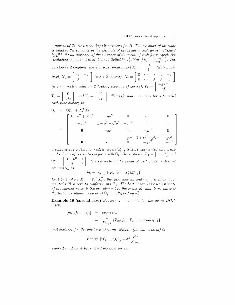
D.3 Recursive least squares 79
a matrix of the corresponding eigenvectors for B. The variance of accrualsis equal to the variance of the estimate of the mean of cash flows multipliedby g2(t−1); the variance of the estimate of the mean of cash flows equals thecoeffi cient on current cash flow multiplied by σ2
e, V ar [m̂t] = numtdentg2
σ2e. The
development employs recursive least squares. Let X1 =
[−ν1
](a 2×1 ma-
trix), X2 =
[gν −ν0 1
](a 2 × 2 matrix), Xt =
[0 · · · 0 gν −ν0 · · · 0 0 1
](a 2 × t matrix with t − 2 leading columns of zeroes), Y1 =
[−gνm0
cf1
],
Y2 =
[0cf2
], and Yt =
[0cft
]. The information matrix for a t-period
cash flow history is
=t = =at−1 +XTt Xt
=
1 + ν2 + g2ν2 −gν2 0 · · · 0
−gν2 1 + ν2 + g2ν2 −gν2 . . ....
0 −gν2 . . . −gν2 0...
. . . −gν2 1 + ν2 + g2ν2 −gν2
0 · · · 0 −gν2 1 + ν2
,
a symmetric tri-diagonal matrix, where =at−1 is =t−1 augmented with a rowand column of zeroes to conform with =t. For instance, =1 =
[1 + ν2
]and
=a1 =
[1 + ν2 0
0 0
]. The estimate of the mean of cash flows is derived
recursively asm̂t = m̂a
t−1 +Kt
(zt −Xa
t m̂at−1
)for t > 1 where Kt = =−1
t XTt , the gain matrix, and m̂
at−1 is m̂t−1 aug-
mented with a zero to conform with m̂t. The best linear unbiased estimateof the current mean is the last element in the vector m̂t and its variance isthe last row-column element of =−1
t multiplied by σ2e.
Example 16 (special case) Suppose g = ν = 1 for the above DGP.Then,
[m̂t|cf1, ..., cft] = accrualst
=1
F2t+1{F2tcft + F2t−1accrualst−1}
and variance for the most recent mean estimate (the tth element) is
V ar [m̂t|cf1, ..., cft]tt = σ2 F2t
F2t+1
where Ft = Ft−1 + Ft−2, the Fibonacci series.

80 Appendix D. Projections and conditional expectations
This is page 81Printer: Opaque this
Appendix E
Two stage least squares IV (2SLS-IV)
In this appendix we develop two stage least squares instrumental variable(2SLS-IV ) estimation more generally. Instrumental variables are attractivestrategies whenever the fundamental condition for regression, E [ε | X] = 0,is violated but we can identify instruments such that E [ε | Z] = 0.
E.1 General case
For the data generating process
Y = Xβ + ε
the IV estimator projects X onto Z (if X includes an intercept so doesZ), X̂ = Z
(ZTZ
)−1ZTX, where X is a matrix of regressors, and Z is a
matrix of instruments. Then, the IV estimator for β is
bIV =(X̂T X̂
)−1
X̂Y
Provided E [ε | Z] = 0 and V ar [ε] = σ2I, bIV is unbiased, E[bIV]
= β,
and has variance V ar[bIV | X,Z
]= σ2
(X̂T X̂
)−1
.
82 Appendix E. Two stage least squares IV (2SLS-IV)
Unbiasedness is demonstrated as follows.
bIV =(X̂T X̂
)−1
X̂Y
=(X̂T X̂
)−1
X̂T (Xβ + ε)
=(XTZ
(ZTZ
)−1ZTZ
(ZTZ
)−1ZTX
)−1
XTZ(ZTZ
)−1ZT (Xβ + ε)
=(XTZ
(ZTZ
)−1ZTX
)−1 (XTZ
(ZTZ
)−1ZTX
)β
+(X̂T X̂
)−1
X̂T ε
= β +(X̂T X̂
)−1
X̂T ε
Then,
E[bIV | X,Z
]= E
[β +
(X̂T X̂
)−1
X̂T ε | X,Z]
= β +(X̂T X̂
)−1
X̂TE [ε | X,Z]
= β + 0 = β
By iterated expectations,
E[bIV]
= EX,Z[E[bIV | X,Z
]]= β
Variance of the IV estimator follows similarly.
V ar[bIV | X,Z
]= E
[(bIV − β
) (bIV − β
)T | X,Z]From the above development,
bIV − β =(X̂T X̂
)−1
X̂T ε
Hence,
V ar[bIV | X,Z
]= E
[(X̂T X̂
)−1
X̂T εεT X̂(X̂T X̂
)−1
| X,Z]
= σ2(X̂T X̂
)−1
X̂T X̂(X̂T X̂
)−1
= σ2(X̂T X̂
)−1
E.2 Special case 83
E.2 Special case
In the special case where both X and Z have the same number of columnsthe estimator can be further simplified,
bIV =(ZTX
)−1ZTY
To see this, write out the estimator
bIV =(X̂T X̂
)−1
X̂Y
=(XTZ
(ZTZ
)−1ZTX
)−1
XTZ(ZTZ
)−1ZTY
Since XTZ and ZTX have linearly independent columns, we can inverteach square term
bIV =(ZTX
)−1ZTZ
(XTZ
)−1XTZ
(ZTZ
)−1ZTY
=(ZTX
)−1ZTY
Of course, the estimator is unbiased, E[bIV]
= β, and the variance of theestimator is
V ar[bIV | X,Z
]= σ2
(X̂T X̂
)−1
which can be written
V ar[bIV | X,Z
]= σ2
(ZTX
)−1ZTZ
(XTZ
)−1
in this special case where X and Z have the same number of columns.

84 Appendix E. Two stage least squares IV (2SLS-IV)
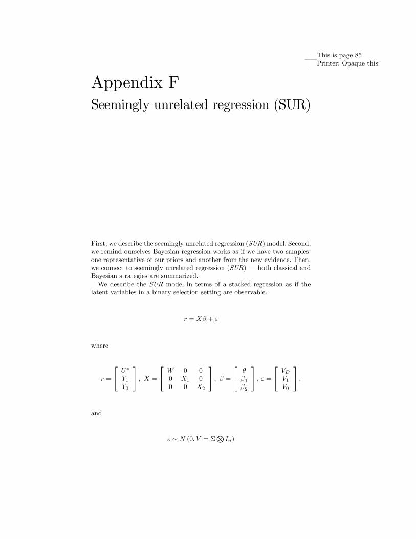
This is page 85Printer: Opaque this
Appendix F
Seemingly unrelated regression (SUR)
First, we describe the seemingly unrelated regression (SUR) model. Second,we remind ourselves Bayesian regression works as if we have two samples:one representative of our priors and another from the new evidence. Then,we connect to seemingly unrelated regression (SUR) – both classical andBayesian strategies are summarized.We describe the SUR model in terms of a stacked regression as if the
latent variables in a binary selection setting are observable.
r = Xβ + ε
where
r =
U∗
Y1
Y0
, X =
W 0 00 X1 00 0 X2
, β =
θβ1
β2
, ε =
VDV1
V0
,
and
ε ∼ N (0, V = Σ⊗In)
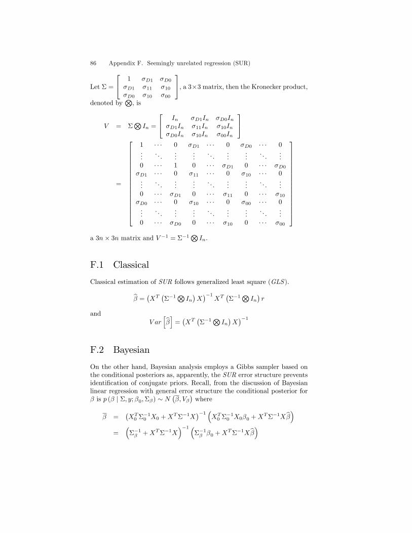
86 Appendix F. Seemingly unrelated regression (SUR)
Let Σ =
1 σD1 σD0
σD1 σ11 σ10
σD0 σ10 σ00
, a 3×3 matrix, then the Kronecker product,
denoted by⊗, is
V = Σ⊗In =
In σD1In σD0InσD1In σ11In σ10InσD0In σ10In σ00In
=
1 · · · 0 σD1 · · · 0 σD0 · · · 0...
. . ....
.... . .
......
. . ....
0 · · · 1 0 · · · σD1 0 · · · σD0
σD1 · · · 0 σ11 · · · 0 σ10 · · · 0...
. . ....
.... . .
......
. . ....
0 · · · σD1 0 · · · σ11 0 · · · σ10
σD0 · · · 0 σ10 · · · 0 σ00 · · · 0...
. . ....
.... . .
......
. . ....
0 · · · σD0 0 · · · σ10 0 · · · σ00
a 3n× 3n matrix and V −1 = Σ−1
⊗In.
F.1 Classical
Classical estimation of SUR follows generalized least square (GLS ).
β̂ =(XT
(Σ−1⊗ In
)X)−1
XT(Σ−1⊗ In
)r
andV ar
[β̂]
=(XT
(Σ−1⊗ In
)X)−1
F.2 Bayesian
On the other hand, Bayesian analysis employs a Gibbs sampler based onthe conditional posteriors as, apparently, the SUR error structure preventsidentification of conjugate priors. Recall, from the discussion of Bayesianlinear regression with general error structure the conditional posterior forβ is p (β | Σ, y;β0,Σβ) ∼ N
(β, Vβ
)where
β =(XT
0 Σ−10 X0 +XTΣ−1X
)−1(XT
0 Σ−10 X0β0 +XTΣ−1Xβ̂
)=
(Σ−1β +XTΣ−1X
)−1 (Σ−1β β0 +XTΣ−1Xβ̂
)
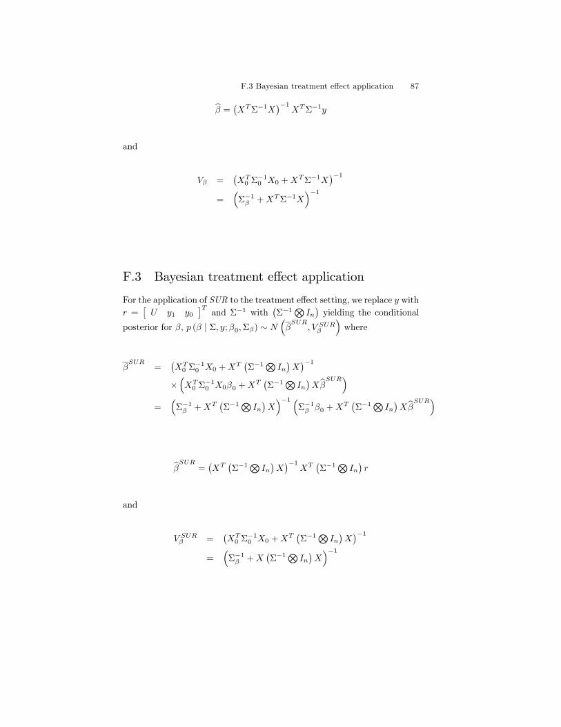
F.3 Bayesian treatment effect application 87
β̂ =(XTΣ−1X
)−1XTΣ−1y
and
Vβ =(XT
0 Σ−10 X0 +XTΣ−1X
)−1
=(
Σ−1β +XTΣ−1X
)−1
F.3 Bayesian treatment effect application
For the application of SUR to the treatment effect setting, we replace y withr =
[U y1 y0
]Tand Σ−1 with
(Σ−1
⊗In)yielding the conditional
posterior for β, p (β | Σ, y;β0,Σβ) ∼ N(βSUR
, V SURβ
)where
βSUR
=(XT
0 Σ−10 X0 +XT
(Σ−1⊗ In
)X)−1
×(XT
0 Σ−10 X0β0 +XT
(Σ−1⊗ In
)Xβ̂
SUR)
=(
Σ−1β +XT
(Σ−1⊗ In
)X)−1 (
Σ−1β β0 +XT
(Σ−1⊗ In
)Xβ̂
SUR)
β̂SUR
=(XT
(Σ−1⊗ In
)X)−1
XT(Σ−1⊗ In
)r
and
V SURβ =(XT
0 Σ−10 X0 +XT
(Σ−1⊗ In
)X)−1
=(
Σ−1β +X
(Σ−1⊗ In
)X)−1

88 Appendix F. Seemingly unrelated regression (SUR)
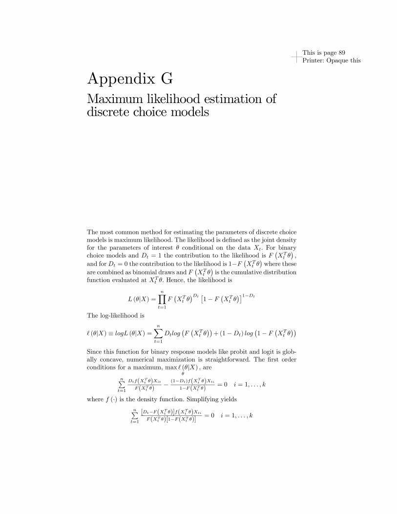
This is page 89Printer: Opaque this
Appendix GMaximum likelihood estimation ofdiscrete choice models
The most common method for estimating the parameters of discrete choicemodels is maximum likelihood. The likelihood is defined as the joint densityfor the parameters of interest θ conditional on the data Xt. For binarychoice models and Dt = 1 the contribution to the likelihood is F
(XTt θ),
and forDt = 0 the contribution to the likelihood is 1−F(XTt θ)where these
are combined as binomial draws and F(XTt θ)is the cumulative distribution
function evaluated at XTt θ. Hence, the likelihood is
L (θ|X) =
n∏t=1
F(XTt θ)Dt [
1− F(XTt θ)]1−Dt
The log-likelihood is
` (θ|X) ≡ logL (θ|X) =
n∑t=1
Dtlog(F(XTt θ))
+ (1−Dt) log(1− F
(XTt θ))
Since this function for binary response models like probit and logit is glob-ally concave, numerical maximization is straightforward. The first orderconditions for a maximum, max ` (θ|X) ,
θ
are
n∑t=1
Dtf(XTt θ)XitF(XTt θ)
− (1−Dt)f(XTt θ)Xti1−F(XTt θ)
= 0 i = 1, . . . , k
where f (·) is the density function. Simplifying yieldsn∑t=1
[Dt−F(XTt θ)]f(XTt θ)Xti
F(XTt θ)[1−F(XTt θ)]= 0 i = 1, . . . , k

90 Appendix G. Maximum likelihood estimation of discrete choice models
Estimates of θ are found by solving these first order conditions iterativelyor, in other words, numerically.A common estimator for the variance of θ̂MLE is the negative inverse of
the Hessian matrix evaluated at θ̂MLE ,[−H
(D, θ̂
)]−1
. Let H (D, θ) be
the Hessian matrix for the log-likelihood with typical element Hij (D, θ) ≡∂2`t(D,θ)∂θi∂θj
.1
1Details can be found in numerous econometrics references and chapter 4 of Account-ing and Causal Eff ects: Econometric Challenges.
This is page 91Printer: Opaque this
Appendix HOptimization
In this appendix, we briefly review optimization. First, we’ll take up linearprogramming then we’ll review nonlinear programming.1
H.1 Linear programming
A linear program (LP) is any optimization frame which can be describedby a linear objective function and linear constraints. Linear refers to choicevariables, say x, of no greater than first degree (affi ne transformations whichallow for parallel lines are included). Prototypical examples are
maxx≥0
πTx
s.t. Ax ≤ r
or
minx≥0
πTx
s.t. Ax ≥ r
1For additional details, consult, for instance, Luenberger and Ye, 2010, Linear andNonlinear Programming, Springer, or Luenberger, 1997 Optimization by Vector SpaceMethods, Wiley.
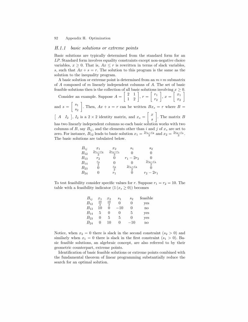
92 Appendix H. Optimization
H.1.1 basic solutions or extreme points
Basic solutions are typically determined from the standard form for anLP. Standard form involves equality constraints except non-negative choicevariables, x ≥ 0. That is, Ax ≤ r is rewritten in terms of slack variables,s, such that Ax + s = r. The solution to this program is the same as thesolution to the inequality program.A basic solution or extreme point is determined from anm×m submatrix
of A composed of m linearly independent columns of A. The set of basicfeasible solutions then is the collection of all basic solutions involving x ≥ 0.
Consider an example. Suppose A =
[2 11 2
], r =
[r1
r2
], x =
[x1
x2
]and s =
[s1
s2
]. Then, Ax + s = r can be written Bxs = r where B =[
A I2], I2 is a 2 × 2 identity matrix, and xs =
[xs
]. The matrix B
has two linearly independent columns so each basic solution works with twocolumns of B, say Bij , and the elements other than i and j of xs are set tozero. For instance, B12 leads to basic solution x1 = 2r1−r2
3 and x2 = 2r2−r13 .
The basic solutions are tabulated below.
Bij x1 x2 s1 s2
B122r1−r2
32r2−r1
3 0 0B13 r2 0 r1 − 2r2 0B14
r12 0 0 2r2−r1
2
B23 0 r22
2r1−r22 0
B24 0 r1 0 r2 − 2r1
To test feasibility consider specific values for r. Suppose r1 = r2 = 10. Thetable with a feasibility indicator (1 (xs ≥ 0)) becomes
Bij x1 x2 s1 s2 feasibleB12
103
103 0 0 yes
B13 10 0 −10 0 noB14 5 0 0 5 yesB23 0 5 5 0 yesB24 0 10 0 −10 no
Notice, when x2 = 0 there is slack in the second constraint (s2 > 0) andsimilarly when x1 = 0 there is slack in the first constraint (s1 > 0). Ba-sic feasible solutions, an algebraic concept, are also referred to by theirgeometric counterpart, extreme points.Identification of basic feasible solutions or extreme points combined with
the fundamental theorem of linear programming substantially reduce thesearch for an optimal solution.
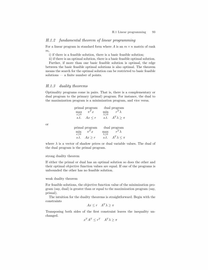
H.1 Linear programming 93
H.1.2 fundamental theorem of linear programming
For a linear program in standard form where A is an m×n matrix of rankm,i) if there is a feasible solution, there is a basic feasible solution;ii) if there is an optimal solution, there is a basic feasible optimal solution.Further, if more than one basic feasible solution is optimal, the edge
between the basic feasible optimal solutions is also optimal. The theoremmeans the search for the optimal solution can be restricted to basic feasiblesolutions – a finite number of points.
H.1.3 duality theorems
Optimality programs come in pairs. That is, there is a complementary ordual program to the primary (primal) program. For instance, the dual tothe maximization program is a minimization program, and vice versa.
primal program dual programmaxx≥0
πTx
s.t. Ax ≤ rminλ≥0
rTλ
s.t. ATλ ≥ π
orprimal program dual programminx≥0
πTx
s.t. Ax ≥ rmaxλ≥0
rTλ
s.t. ATλ ≤ π
where λ is a vector of shadow prices or dual variable values. The dual ofthe dual program is the primal program.
strong duality theorem
If either the primal or dual has an optimal solution so does the other andtheir optimal objective function values are equal. If one of the programs isunbounded the other has no feasible solution.
weak duality theorem
For feasible solutions, the objective function value of the minimization pro-gram (say, dual) is greater than or equal to the maximization program (say,primal).The intuition for the duality theorems is straightforward. Begin with the
constraintsAx ≤ r ATλ ≥ π
Transposing both sides of the first constraint leaves the inequality un-changed.
xTAT ≤ rT ATλ ≥ π
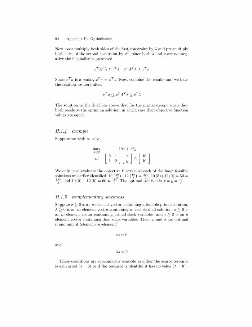
94 Appendix H. Optimization
Now, post-multiply both sides of the first constraint by λ and pre-multiplyboth sides of the second constraint by xT , since both λ and x are nonneg-ative the inequality is preserved.
xTATλ ≤ rTλ xTATλ ≥ xTπ
Since xTπ is a scalar, xTπ = πTx. Now, combine the results and we havethe relation we were after.
πTx ≤ xTATλ ≤ rTλ
The solution to the dual lies above that for the primal except when theyboth reside at the optimum solution, in which case their objective functionvalues are equal.
H.1.4 example
Suppose we wish to solve
maxx≥0
10x+ 12y
s.t
[2 11 2
] [xy
]≤[
1010
]We only need evaluate the objective function at each of the basic feasiblesolutions we earlier identified: 10
(103
)+12
(103
)= 220
3 , 10 (5)+12 (0) = 50 =1503 , and 10 (0) + 12 (5) = 60 = 180
3 . The optimal solution is x = y = 103 .
H.1.5 complementary slackness
Suppose x ≥ 0 is an n element vector containing a feasible primal solution,λ ≥ 0 is an m element vector containing a feasible dual solution, s ≥ 0 isan m element vector containing primal slack variables, and t ≥ 0 is an nelement vector containing dual slack variables. Then, x and λ are optimalif and only if (element-by-element)
xt = 0
and
λs = 0
These conditions are economically sensible as either the scarce resourceis exhausted (s = 0) or if the resource is plentiful it has no value (λ = 0).
H.2 Nonlinear programming 95
H.2 Nonlinear programming
H.2.1 unconstrained
Nonlinear programs involve nonlinear objective functions. For instance,
maxx
f (x)
If the function is continuously differentiable, then a local optimum can befound by the first order approach. That is, equate the gradient (a vector ofpartial derivatives composed of terms, ∂f(x)
∂xi, i = 1, . . . , n where there are
n choice variables, x).
∇f (x∗) = 0∂f(x)∂x1...
∂f(x)∂xn
=
0...0
Second order (suffi cient) conditions involve the Hessian, a matrix of secondpartial derivatives.
H (x∗) =
∂2f(x)∂x1∂x1
· · · ∂2f(x)∂x1∂xn
.... . .
...∂2f(x)∂xn∂x1
· · · ∂2f(x)∂xn∂xn
For a local minimum, the Hessian is positive definite (the eigenvalues of Hare positive). While for a local maximum, the Hessian is negative definite(the eigenvalues of H are negative).
H.2.2 convexity and global minima
If f is a convex function (defined below), then the set where f achieves itslocal minimum is convex and any local minimum is a global minimum. Afunction f is convex if for every x1, x2, and α , 0 ≤ α ≤ 1,
f (αx1 + (1− α)x2) ≤ αf (x1) + (1− α) f (x2)
If x1 6= x2, and 0 < α < 1,
f (αx1 + (1− α)x2) < αf (x1) + (1− α) f (x2)
then f is strictly convex. If g = −f and f is (strictly) convex, then g is(strictly) concave.
96 Appendix H. Optimization
H.2.3 example
Suppose we face the problem
minx,y
f (x, y) = x2 − 10x+ y2 − 10y + xy
The first order conditions are
∇f (x, y) = 0
or
∂f
∂x= 2x− 10 + y = 0
∂f
∂y= 2y − 10 + x = 0
Since the problem is quadratic and the gradient is composed of linearlyindependent equations, a unique solution is immediately identifiable.[
2 11 2
] [xy
]=
[1010
]or x = y = 10
3 with objective function value −1003 . As the Hessian is positive
definite, this solution is a minimum.
H =
[2 11 2
]Positive definiteness of the Hessian follows as the eigenvalues of H arepositive. To see this, recall the sum of the eigenvalues equals the trace ofthe matrix and the product of the eigenvalues equals the determinant ofthe matrix. The eigenvalues of H are 1 and 3, both positive.
H.2.4 constrained – the Lagrangian
Nonlinear programs involve either nonlinear objective functions, constraints,or both. For instance,
maxx≥0
f (x)
s.t. G (x) ≤ rSuppose the objective function and constraints are continuously differ-
entiable concave and an optimal solution exists, then the optimal solutioncan be found via the Lagrangian. The Lagrangian writes the objective func-tion less a Lagrange multiplier times each of the constraints. As either themultiplier is zero or the constraint is binding, each constraint term equalszero.
L = f (x)− λ1 [g1 (x)− r1]− · · · − λn [gn (x)− rn]
H.2 Nonlinear programming 97
where G (x) involves n functions, gi (x), i = 1, . . . , n. Suppose x involvesm choice variables. Then, there are m Lagrange equations plus the n con-straints that determine the optimal solution.
∂L∂x1
= 0
...∂L∂xm
= 0
λ1 [g1 (x)− r1] = 0
...
λn [gn (x)− rn] = 0
The Lagrange multipliers (shadow prices or dual variable values) repre-sent the rate of change in the optimal objective function for each of theconstraints.
λi =∂f (r∗)
∂ri
where r∗ refers to rewriting the optimal solution x∗ in terms of the con-straint values, r. If a constraint is not binding, it’s multiplier is zero as ithas no impact on the optimal objective function value.2
H.2.5 Karash-Kuhn-Tucker conditions
Originally, the Lagrangian only allowed for equality constraints. This wasgeneralized to include inequality constraints by Karash and separatelyKuhn and Tucker. Of course, some regularity conditions are needed toensure optimality. Various necessary and suffi cient conditions have beenproposed to deal with the most general settings. The Karash-Kuhn-Tuckertheorem supplies first order necessary conditions for a local optimum (gra-dient of the Lagrangian and the Lagrange multiplier times the inequalityconstraint equal zero when the Lagrange multipliers on the inequality con-straints are non-negative evaluated at x∗). Second order necessary (positivesemi-definite Hessian for the Lagrangian at x∗) and suffi cient (positive def-inite Hessian for the Lagrangian at x∗) conditions are roughly akin to thosefor unconstrained local minima.
2Of course, these ideas regarding the multipliers apply to the shadow prices of linearprograms as well.
98 Appendix H. Optimization
H.2.6 example
Continue with the unconstrained example above with an added constraint.
minx,y
f (x, y) = x2 − 10x+ y2 − 10y + xy
s.t. xy ≥ 10
Since the unconstrained solution satisfies this constraint, xy = 1009 > 10,
the solution remains x = y = 103 .
However, suppose the problem is
minx,y
f (x, y) = x2 − 10x+ y2 − 10y + xy
s.t. xy ≥ 20
The constraint is now active. The Lagrangian is
L = x2 − 10x+ y2 − 10y + xy − λ (xy − 20)
and the first order conditions are
∇L = 0
or
∂L∂x
= 2x− 10 + y − λy = 0
∂L∂y
= 2y − 10 + x− λx = 0
and constraint equation
λ (xy − 20) = 0
A solution to these nonlinear equations is
x = y = 2√
5
λ = 3−√
5
The objective function value is −29.4427 which, of course, is greater thanthe objective function value for the unconstrained problem, −33.3333. TheHessian is
H =
[2 1− λ
1− λ 2
]with eigenvalues evaluated at the solution, 3−λ =
√5 and 1 +λ = 4−
√5,
both positive. Hence, the solution is a minimum.
H.3 Theorem of the separating hyperplane 99
H.3 Theorem of the separating hyperplane
The theorem of the separating hyperplane states either there exists a non-negative y such that Ay = x or there exists λ such that ATλ ≥ 0 andλTx < 0. The theorem is about mutual exclusivity – one or the other istrue not both. This is similar to the way in which orthogonal complementsare mutually exclusive. If one subspace contains all positive vectors theorthogonal complement cannot contain positive vectors. Otherwise, theirinner products would be positive and inner products of orthogonal sub-spaces are zero.The intuition follows from the idea that vector inner products are pro-
portional to the cosine of the angle between them; if the angle is less(greater) than 90 degrees the cosine is positive (negative). ATλ ≥ 0 meansthe columns of A are less than or equal to 90 degrees relative a fixed vectorλ while λTx < 0 implies the angle between x and λ exceeds 90 degrees. Theseparating hyperplane (hyper simply refers to high dimension) is composedof all vectors orthogonal to a fixed vector λ.Consider a simple example.
Example 17 (simple example) Suppose A = I and x =
[23
], then
y = 2
[10
]+ 3
[01
]and there exists no λ from which to form a plane
separating the positive quadrant from x. On the other hand, suppose x =[−23
]– x lies outside the positive quadrant and λ =
[10
]satisfies the
theorem’s alternative, ATλ =
[10
]≥ 0 and λTx = −2 < 0.
Next, consider a simple accounting (incidence matrix) example. That is,a case in which A has a nullspace and a left nullspace.
Example 18 (simple accounting example) If A =
−1 0 11 −1 00 1 −1
and x =
12−3
, then y =
203
+ k
111
and any k ≥ 0 satisfies
Ay = x and y ≥ 0. Hence, there exists no separating plane based on λ.
On the other hand, suppose A =
−1 0 −11 −1 00 1 1
. Now, y =
20−3
+
k
11−1
and no k satisfies Ay = x and y ≥ 0. Any number of λs exist.
100 Appendix H. Optimization
For example, λ =
001
produces ATλ =
011
≥ 0 and λTx = −3 < 0.
Hence, any λ =
001
+k
111
(drawing on the left nullspace of A) wherek > −1 satisfies the theorem’s alternative.
This is page 101Printer: Opaque this
Appendix IQuantum information
Quantum information follows from physical theory and experiments. Un-like classical information which is framed in the language and algebra ofset theory, quantum information is framed in the language and algebra ofvector spaces. To begin to appreciate the difference, consider a set versusa tuple (or vector). For example, the tuple
[1 1
]is different than the
tuple[
1 1 1]but the sets, {1, 1} and {1, 1, 1} are the same as set {1}.
Quantum information is axiomatic. Its richness and elegance is demon-strated in that only four axioms make it complete.1
I.1 Quantum information axioms
I.1.1 The superposition axiom
A quantum unit (qubit) is specified by a two element vector, say[αβ
],
with |α|2 + |β|2 = 1.
1Some argue that the measurement axiom is contained in the transformation ax-iom, hence requiring only three axioms. Even though we appreciate the merits of theargument, we’ll proceed with four axioms. Feel free to count them as only three if youprefer.
102 Appendix I. Quantum information
Let |ψ〉 ≡[αβ
]= α |0〉 + β |1〉,2 〈ψ| =
[αβ
]†where † is the adjoint
(conjugate transpose) operation.
I.1.2 The transformation axiom
A transformation of a quantum unit is accomplished by unitary (length-preserving) matrix multiplication. The Pauli matrices provide a basis ofunitary operators.
I =
[1 00 1
]X =
[0 11 0
]Y =
[0 −ii 0
]Z =
[1 00 −1
]
where i =√−1. The operations work as follows: I
[αβ
]=
[αβ
],X[αβ
]=[
βα
], Y
[αβ
]= −
[βiαi
], and Z
[αβ
]= −
[αβ
]. Other useful sin-
gle qubit transformations are H = 1√2
[1 11 −1
]and Θ =
[eiθ 00 1
].
Examples of these transformations in Dirac notation are3
H |0〉 =|0〉+ |1〉√
2; H |1〉 =
|0〉 − |1〉√2
Θ |0〉 = eiθ |0〉 ; Θ |1〉 = |1〉
I.1.3 The measurement axiom
Measurement occurs via interaction with the quantum state as if a linearprojection is applied to the quantum state.4 The set of projection matrices
2Dirac notation is a useful descriptor, as |0〉 =[10
]and |1〉 =
[01
].
3A summary table for common quantum operators expressed in Dirac notation isprovided in section I.2.
4This is a compact way of describing measurement. However, conservation of infor-mation (a principle of quantum information) demands that operations be reversible.In other words, all transformations (including interactions to measure) be unitary –projections are not unitary. However, there always exist unitary operators that pro-duce the same post-measurement state as that indicated via projection. Hence, we treatprojections as an expedient for describing measurement.
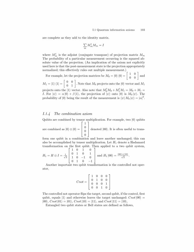
I.1 Quantum information axioms 103
are complete as they add to the identity matrix.∑mM†mMm = I
where M†m is the adjoint (conjugate transpose) of projection matrix Mm
The probability of a particular measurement occurring is the squared ab-solute value of the projection. (An implication of the axiom not explicitlyused here is that the post-measurement state is the projection appropriatelynormalized; this effectively rules out multiple measurement.)
For example, let the projection matrices beM0 = |0〉 〈0| =[
1 00 0
]and
M1 = |1〉 〈1| =[
0 00 1
]. Note thatM0 projects onto the |0〉 vector andM1
projects onto the |1〉 vector. Also note that M†0M0 +M†1M1 = M0 +M1 =I. For |ψ〉 = α |0〉 + β |1〉, the projection of |ψ〉 onto |0〉 is M0 |ψ〉. Theprobability of |0〉 being the result of the measurement is 〈ψ|M0 |ψ〉 = |α|2.
I.1.4 The combination axiom
Qubits are combined by tensor multiplication. For example, two |0〉 qubits
are combined as |0〉 ⊗ |0〉 =
1000
denoted |00〉. It is often useful to trans-
form one qubit in a combination and leave another unchanged; this canalso be accomplished by tensor multiplication. Let H1 denote a Hadamardtransformation on the first qubit. Then applied to a two qubit system,
H1 = H ⊗ I = 1√2
1 0 1 00 1 0 11 0 −1 00 1 0 −1
and H1 |00〉 = |00〉+|10〉√2
.
Another important two qubit transformation is the controlled not oper-ator,
Cnot =
1 0 0 00 1 0 00 0 0 10 0 1 0
The controlled not operator flips the target, second qubit, if the control, firstqubit, equals |1〉 and otherwise leaves the target unchanged: Cnot |00〉 =|00〉, Cnot |01〉 = |01〉, Cnot |10〉 = |11〉, and Cnot |11〉 = |10〉,Entangled two qubit states or Bell states are defined as follows,

104 Appendix I. Quantum information
|β00〉 = Cnot H1 |00〉 =|00〉+ |11〉√
2
and more generally,
∣∣βij⟩ = Cnot H1 |ij〉 for i, j = 0, 1
The four two qubit Bell states form an orthonormal basis.
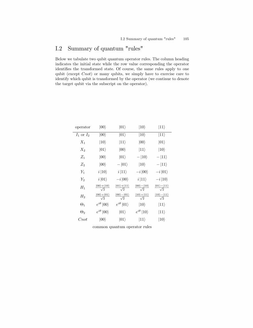
I.2 Summary of quantum "rules" 105
I.2 Summary of quantum "rules"
Below we tabulate two qubit quantum operator rules. The column headingindicates the initial state while the row value corresponding the operatoridentifies the transformed state. Of course, the same rules apply to onequbit (except Cnot) or many qubits, we simply have to exercise care toidentify which qubit is transformed by the operator (we continue to denotethe target qubit via the subscript on the operator).
operator |00〉 |01〉 |10〉 |11〉
I1 or I2 |00〉 |01〉 |10〉 |11〉
X1 |10〉 |11〉 |00〉 |01〉
X2 |01〉 |00〉 |11〉 |10〉
Z1 |00〉 |01〉 − |10〉 − |11〉
Z2 |00〉 − |01〉 |10〉 − |11〉
Y1 i |10〉 i |11〉 −i |00〉 −i |01〉
Y2 i |01〉 −i |00〉 i |11〉 −i |10〉
H1|00〉+|10〉√
2
|01〉+|11〉√2
|00〉−|10〉√2
|01〉−|11〉√2
H2|00〉+|01〉√
2
|00〉−|01〉√2
|10〉+|11〉√2
|10〉−|11〉√2
Θ1 eiθ |00〉 eiθ |01〉 |10〉 |11〉
Θ2 eiθ |00〉 |01〉 eiθ |10〉 |11〉
Cnot |00〉 |01〉 |11〉 |10〉
common quantum operator rules
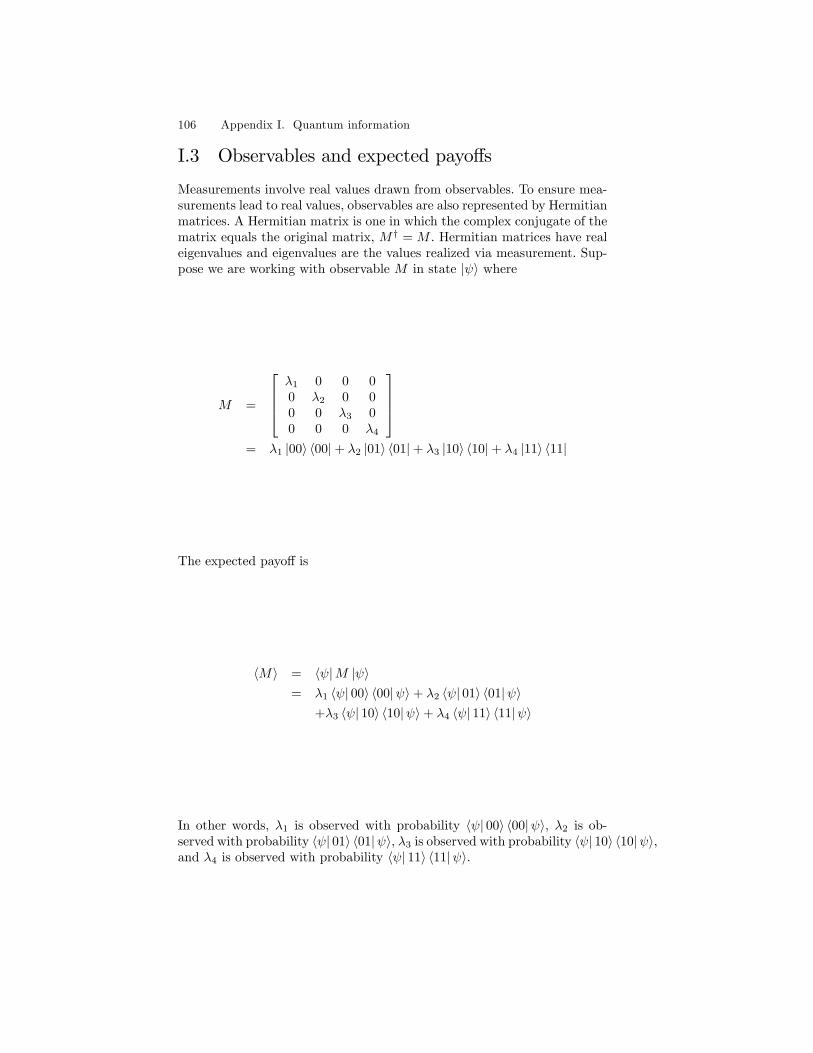
106 Appendix I. Quantum information
I.3 Observables and expected payoffs
Measurements involve real values drawn from observables. To ensure mea-surements lead to real values, observables are also represented by Hermitianmatrices. A Hermitian matrix is one in which the complex conjugate of thematrix equals the original matrix, M† = M . Hermitian matrices have realeigenvalues and eigenvalues are the values realized via measurement. Sup-pose we are working with observable M in state |ψ〉 where
M =
λ1 0 0 00 λ2 0 00 0 λ3 00 0 0 λ4
= λ1 |00〉 〈00|+ λ2 |01〉 〈01|+ λ3 |10〉 〈10|+ λ4 |11〉 〈11|
The expected payoff is
〈M〉 = 〈ψ|M |ψ〉= λ1 〈ψ| 00〉 〈00|ψ〉+ λ2 〈ψ| 01〉 〈01|ψ〉
+λ3 〈ψ| 10〉 〈10|ψ〉+ λ4 〈ψ| 11〉 〈11|ψ〉
In other words, λ1 is observed with probability 〈ψ| 00〉 〈00|ψ〉, λ2 is ob-served with probability 〈ψ| 01〉 〈01|ψ〉, λ3 is observed with probability 〈ψ| 10〉 〈10|ψ〉,and λ4 is observed with probability 〈ψ| 11〉 〈11|ψ〉.
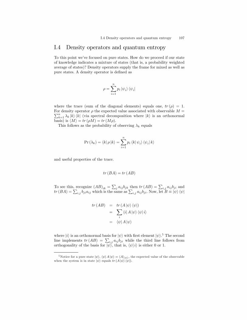
I.4 Density operators and quantum entropy 107
I.4 Density operators and quantum entropy
To this point we’ve focused on pure states. How do we proceed if our stateof knowledge indicates a mixture of states (that is, a probability weightedaverage of states)? Density operators supply the frame for mixed as well aspure states. A density operator is defined as
ρ =
n∑i=1
pi |ψi〉 〈ψi|
where the trace (sum of the diagonal elements) equals one, tr (ρ) = 1.For density operator ρ the expected value associated with observable M =∑nk=1 λk |k〉 〈k| (via spectral decomposition where |k〉 is an orthonormal
basis) is 〈M〉 = tr (ρM) = tr (Mρ).This follows as the probability of observing λk equals
Pr (λk) = 〈k| ρ |k〉 =
n∑i=1
pi 〈k|ψi〉 〈ψi| k〉
and useful properties of the trace.
tr (BA) = tr (AB)
To see this, recognize (AB)ik =∑j aijbjk then tr (AB) =
∑i,j aijbji and
tr (BA) =∑i,j bjiaij which is the same as
∑i,j aijbji. Now, let B ≡ |ψ〉 〈ψ|
tr (AB) = tr (A |ψ〉 〈ψ|)=
∑i
〈i|A |ψ〉 〈ψ| i〉
= 〈ψ|A |ψ〉
where |i〉 is an orthonormal basis for |ψ〉 with first element |ψ〉.5 The secondline implements tr (AB) =
∑i,j aijbji while the third line follows from
orthogonality of the basis for |ψ〉, that is, 〈ψ| i〉 is either 0 or 1.
5Notice for a pure state |ψ〉, 〈ψ|A |ψ〉 = 〈A〉|ψ〉, the expected value of the observablewhen the system is in state |ψ〉 equals tr (A |ψ〉 〈ψ|).
108 Appendix I. Quantum information
Then, applying the first result followed by the third result in reverse andrepeating based on the second result we have
〈M〉 =
n∑k=1
Pr (λk)λk
=
n∑k=1
n∑i=1
pi 〈k|ψi〉 〈ψi| k〉λk
=
n∑k=1
〈k| ρ |k〉λk
= tr (Mρ)
=n∑k=1
n∑i=1
pi 〈ψi| k〉 〈k|ψi〉λk
=
n∑i=1
pi 〈ψi|M |ψi〉
= tr (ρM)
Consider an example. Suppose
ρ =
[0.4 00 0.6
]= 0.4
[10
] [1 0
]+ 0.6
[01
] [0 1
]and
M =
[1 −2−2 1
]= 3
[1√2
− 1√2
] [1√2− 1√
2
]− 1
[1√2
1√2
] [1√2
1√2
]
Then,
Pr (λ = 3) =[
1√2− 1√
2
] [0.4 00 0.6
] [ 1√2
− 1√2
]
= 0.4[
1√2− 1√
2
] [10
] [1 0
] [ 1√2
− 1√2
]
+0.6[
1√2− 1√
2
] [ 01
] [0 1
] [ 1√2
− 1√2
]
=1
2
I.4 Density operators and quantum entropy 109
and
Pr (λ = −1) =[
1√2
1√2
] [ 0.4 00 0.6
][ 1√2
1√2
]
= 0.4[
1√2
1√2
] [10
] [1 0
] [ 1√2
1√2
]
+0.6[
1√2
1√2
] [ 01
] [0 1
] [ 1√2
1√2
]
=1
2
Hence, the expected value for the observable M is
〈M〉 =
2∑k=1
Pr (λk)λk
=1
23 +
1
2(−1) = 1
= tr (ρM) = tr (Mρ)
=
[0.4 −0.8−1.2 0.6
]=
[0.4 −1.2−0.8 0.6
]= 1
or
〈M〉 =∑i,j
pj 〈i|M |ψ〉 〈ψ| i〉
= 0.4[
1 0] [ 1 −2−2 1
] [10
] [1 0
] [ 10
]+0.4
[0 1
] [ 1 −2−2 1
] [10
] [1 0
] [ 01
]0.6[
1 0] [ 1 −2−2 1
] [01
] [0 1
] [ 10
]+0.6
[0 1
] [ 1 −2−2 1
] [01
] [0 1
] [ 01
]=
∑j
pj 〈ψ|M |ψ〉
= 0.4[
1 0] [ 1 −2−2 1
] [10
]+0.6
[0 1
] [ 1 −2−2 1
] [01
]= 0.4 + 0.6 = 1
110 Appendix I. Quantum information
I.4.1 Quantum entropy
von Neumann defines quantum entropy as
S = −tr (ρ log ρ)
For pure states, ρ is a Hermitian matrix whose logarithm (discussed earlier)involves its spectral decomposition ρ = QΛQT where Λ has one eigenvalueequal to unity and the remainder equal to zero. Hence, log ρ = Q log ΛQT =0 (by convention, 0 log 0 = 0) so that von Neumann entropy is zero for purestates.On the other hand, for mixed states spectral decomposition of ρ is∑nj=1 λj |j〉 〈j|. This involves nonzero eigenvalues so that
S = −tr (ρ log ρ)
= −tr
n∑j=1
λj |j〉 〈j|n∑j=1
log (λj) |j〉 〈j|
= −tr
n∑j=1
λj log (λj) |j〉 〈j| |j〉 〈j|
= −tr
n∑j=1
λj log (λj) |j〉 〈j|
= −
n∑i=1
λi log λi
The latter result follows from equality of the sum of the eigenvalues andthe trace of a matrix.
I.5 Some trigonometric identities
Most trigonometric identities follow directly from Euler’s equation:
e±iθ = cos θ ± i sin θ
Remark 1 cos2 θ + sin2 θ = 1
Proof.
eiθe−iθ = e0 = 1
(cos θ + i sin θ) (cos θ − i sin θ) = cos2 θ + i cos θ sin θ − i cos θ sin θ + sin2 θ
= cos2 θ + sin2 θ
I.5 Some trigonometric identities 111
Remark 2 1−cos θ2 = sin2 θ
2
Proof.
2−(eiθ + e−iθ
)4
=2− 2 cos θ
4=
1− cos θ
2
2−[(eiθ2
)2
+(e−
iθ2
)2]
4=
2−[2− 4 sin2 θ
2
]4
= sin2 θ
2
Details related to the second line are below.
(eiθ2
)2
=
(cos
θ
2+ i sin
θ
2
)2
= cos2 θ
2− sin2 θ
2+ 2i cos
θ
2sin
θ
2
(e−
iθ2
)2
=
(cos
θ
2− i sin
θ
2
)2
= cos2 θ
2− sin2 θ
2− 2i cos
θ
2sin
θ
2
(eiθ2
)2
+(e−
iθ2
)2
= 2 cos2 θ
2− 2 sin2 θ
2
= 2− 4 sin2 θ
2
Remark 3 1−cos θ1 cos θ22 = cos2 θ1
2 sin2 θ22 + sin2 θ1
2 cos2 θ22
Proof. From the two preceding identities
1− cos θ
2= sin2 θ
2= 1− cos2 θ
2
and
cos θ = 1− 2 sin2 θ
2
= 2 cos2 θ
2− 1
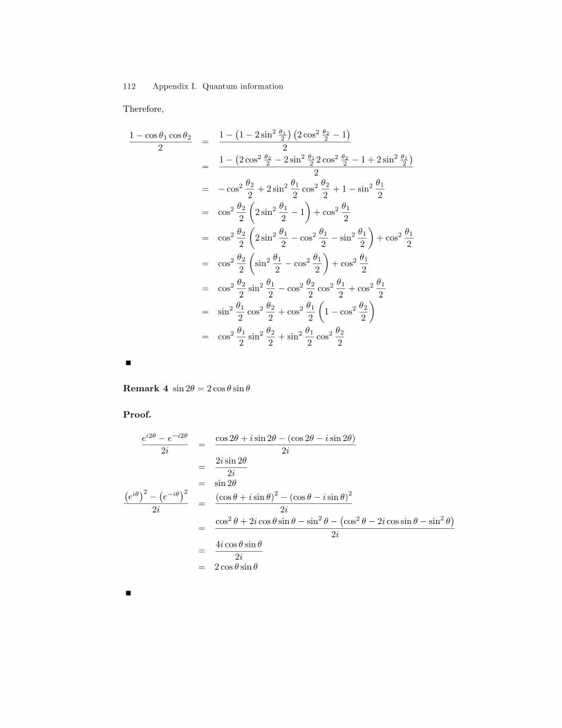
112 Appendix I. Quantum information
Therefore,
1− cos θ1 cos θ2
2=
1−(1− 2 sin2 θ1
2
) (2 cos2 θ2
2 − 1)
2
=1−
(2 cos2 θ2
2 − 2 sin2 θ12 2 cos2 θ2
2 − 1 + 2 sin2 θ12
)2
= − cos2 θ2
2+ 2 sin2 θ1
2cos2 θ2
2+ 1− sin2 θ1
2
= cos2 θ2
2
(2 sin2 θ1
2− 1
)+ cos2 θ1
2
= cos2 θ2
2
(2 sin2 θ1
2− cos2 θ1
2− sin2 θ1
2
)+ cos2 θ1
2
= cos2 θ2
2
(sin2 θ1
2− cos2 θ1
2
)+ cos2 θ1
2
= cos2 θ2
2sin2 θ1
2− cos2 θ2
2cos2 θ1
2+ cos2 θ1
2
= sin2 θ1
2cos2 θ2
2+ cos2 θ1
2
(1− cos2 θ2
2
)= cos2 θ1
2sin2 θ2
2+ sin2 θ1
2cos2 θ2
2
Remark 4 sin 2θ = 2 cos θ sin θ
Proof.
ei2θ − e−i2θ2i
=cos 2θ + i sin 2θ − (cos 2θ − i sin 2θ)
2i
=2i sin 2θ
2i= sin 2θ(
eiθ)2 − (e−iθ)2
2i=
(cos θ + i sin θ)2 − (cos θ − i sin θ)
2
2i
=cos2 θ + 2i cos θ sin θ − sin2 θ −
(cos2 θ − 2i cos sin θ − sin2 θ
)2i
=4i cos θ sin θ
2i= 2 cos θ sin θ

This is page 113Printer: Opaque this
Appendix JCommon distributions
To try to avoid confusion, we list our descriptions of common multivariateand univariate distributions and their kernels. Others may employ varia-tions on these definitions.
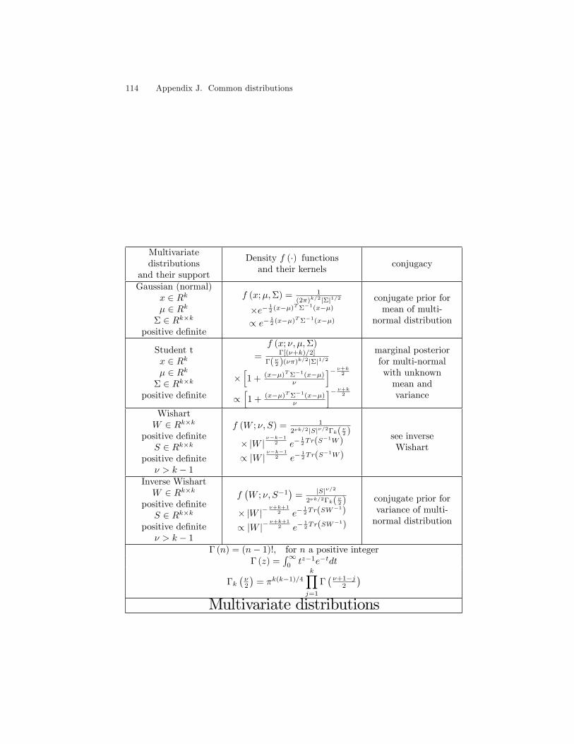
114 Appendix J. Common distributions
Multivariatedistributions
and their support
Density f (·) functionsand their kernels
conjugacy
Gaussian (normal)x ∈ Rkµ ∈ Rk
Σ ∈ Rk×kpositive definite
f (x;µ,Σ) = 1(2π)k/2|Σ|1/2
×e− 12 (x−µ)TΣ−1(x−µ)
∝ e− 12 (x−µ)TΣ−1(x−µ)
conjugate prior formean of multi-
normal distribution
Student tx ∈ Rkµ ∈ Rk
Σ ∈ Rk×kpositive definite
f (x; ν, µ,Σ)
= Γ[(ν+k)/2]
Γ( ν2 )(νπ)k/2|Σ|1/2
×[1 + (x−µ)TΣ−1(x−µ)
ν
]− ν+k2∝[1 + (x−µ)TΣ−1(x−µ)
ν
]− ν+k2marginal posteriorfor multi-normalwith unknownmean andvariance
WishartW ∈ Rk×k
positive definiteS ∈ Rk×k
positive definiteν > k − 1
f (W ; ν, S) = 1
2νk/2|S|ν/2Γk( ν2 )
× |W |ν−k−1
2 e−12Tr(S
−1W)
∝ |W |ν−k−1
2 e−12Tr(S
−1W)
see inverseWishart
Inverse WishartW ∈ Rk×k
positive definiteS ∈ Rk×k
positive definiteν > k − 1
f(W ; ν, S−1
)= |S|ν/2
2νk/2Γk( ν2 )
× |W |−ν+k+1
2 e−12Tr(SW
−1)
∝ |W |−ν+k+1
2 e−12Tr(SW
−1)
conjugate prior forvariance of multi-normal distribution
Γ (n) = (n− 1)!, for n a positive integerΓ (z) =
∫∞0tz−1e−tdt
Γk(ν2
)= πk(k−1)/4
k∏j=1
Γ(ν+1−j
2
)Multivariate distributions
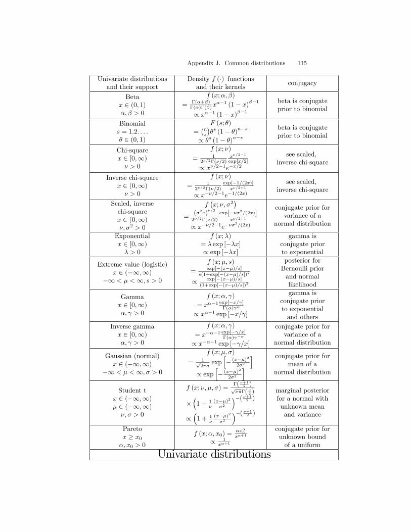
Appendix J. Common distributions 115
Univariate distributionsand their support
Density f (·) functionsand their kernels
conjugacy
Betax ∈ (0, 1)α, β > 0
f (x;α, β)
= Γ(α+β)Γ(α)Γ(β)x
α−1 (1− x)β−1
∝ xα−1 (1− x)β−1
beta is conjugateprior to binomial
Binomials = 1.2. . . .θ ∈ (0, 1)
F (s; θ)
=(ns
)θs (1− θ)n−s
∝ θs (1− θ)n−sbeta is conjugateprior to binomial
Chi-squarex ∈ [0,∞)ν > 0
f (x; ν)
= 12ν/2Γ(ν/2)
xν/2−1
exp[x/2]
∝ xν/2−1e−x/2
see scaled,inverse chi-square
Inverse chi-squarex ∈ (0,∞)ν > 0
f (x; ν)
= 12ν/2Γ(ν/2)
exp[−1/(2x)]xν/2+1
∝ x−ν/2−1e−1/(2x)
see scaled,inverse chi-square
Scaled, inversechi-squarex ∈ (0,∞)ν, σ2 > 0
f(x; ν, σ2
)=
(σ2ν)ν/2
2ν/2Γ(ν/2)
exp[−νσ2/(2x)]xν/2+1
∝ x−ν/2−1e−νσ2/(2x)
conjugate prior forvariance of a
normal distribution
Exponentialx ∈ [0,∞)λ > 0
f (x;λ)= λ exp [−λx]∝ exp [−λx]
gamma isconjugate priorto exponential
Extreme value (logistic)x ∈ (−∞,∞)
−∞ < µ <∞, s > 0
f (x;µ, s)
= exp[−(x−µ)/s]
s(1+exp[−(x−µ)/s])2
∝ exp[−(x−µ)/s]
(1+exp[−(x−µ)/s])2
posterior forBernoulli priorand normallikelihood
Gammax ∈ [0,∞)α, γ > 0
f (x;α, γ)
= xα−1 exp[−x/γ]Γ(α)γα
∝ xα−1 exp [−x/γ]
gamma isconjugate priorto exponentialand others
Inverse gammax ∈ [0,∞)α, γ > 0
f (x;α, γ)
= x−α−1 exp[−γ/x]Γ(α)γ−α
∝ x−α−1 exp [−γ/x]
conjugate prior forvariance of a
normal distribution
Gaussian (normal)x ∈ (−∞,∞)
−∞ < µ <∞, σ > 0
f (x;µ, σ)
= 1√2πσ
exp[− (x−µ)2
2σ2
]∝ exp
[− (x−µ)2
2σ2
] conjugate prior formean of a
normal distribution
Student tx ∈ (−∞,∞)µ ∈ (−∞,∞)ν, σ > 0
f (x; ν, µ, σ) =Γ( ν+12 )√νπΓ( ν2 )
×(
1 + 1ν
(x−µ)2
σ2
)−( ν+12 )
∝(
1 + 1ν
(x−µ)2
σ2
)−( ν+12 )
marginal posteriorfor a normal withunknown meanand variance
Paretox ≥ x0
α, x0 > 0
f (x;α, x0) =αxα0xα+1
∝ 1xα+1
conjugate prior forunknown boundof a uniform
Univariate distributions