Content and task-based view selection from multiple video ...andrea/papers/2009_MTA_SelectionMultipleVideo... · Content and task-based view selection from multiple video streams

Content and task-based view selection from multiple videostreams

Fahad Daniyal · Murtaza Taj · Andrea Cavallaro

Received: date / Accepted: date

Abstract We present a content-aware multi-camera selection technique that uses object-and frame-level features. First objects are detected using a color-based change detector.Next trajectory information for each object is generated using multi-frame graph matching.Finally, multiple features including size and location are used to generate an object score.At frame-level, we consider total activity, event score, number of objects and cumulativeobject score. These features are used to generate score information using a multivariateGaussian distribution. The algorithm. The best view is selected using a Dynamic BayesianNetwork (DBN), which utilizes camera network information. DBN employs previous viewinformation to select the current view thus increasing resilience to frequent switching. Theperformance of the proposed approach is demonstrated on three multi-camera setups withsemi-overlapping fields of view: a basketball game, an indoor airport surveillance scenarioand a synthetic outdoor pedestrian dataset. We compare the proposed view selection ap-proach with a maximum score based camera selection criterion and demonstrate a significantdecrease in camera flickering. The performance of the proposed approach is also validatedthrough subjective testing.

Keywords Content scoring · information ranking · feature analysis · camera selection ·content analysis · autonomous video production

1 Introduction

Multi-camera settings are becoming increasingly common in scenarios ranging from sportsto surveillance and smart meeting rooms. An important task is the quantification of viewquality to help select a single camera or a subset of cameras for optimal observability. The

F. DaniyalMultimedia and Vision Group - Queen Mary University of London, United Kingdom, E1 4NS, UKTel.: +44-20-7882-5259E-mail: [email protected]

M. TajE-mail: [email protected]

A. CavallaroE-mail: [email protected]

MULTIMEDIA TOOLS AND APPLICATIONS, ARTICLE ID 5872291, SEPTEMBER 2009

2

contextualco te tuainformation

featureextraction

contentscoring1C

camera selection

g

contentscoring2C feature

extractionC~

contentscoring

featureextractionNC

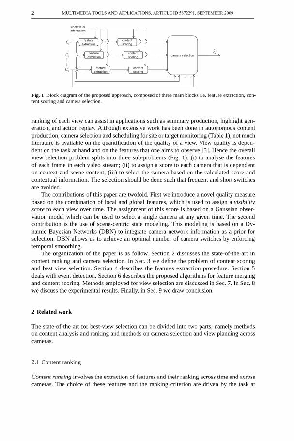
Fig. 1 Block diagram of the proposed approach, composed of three main blocks i.e. feature extraction, con-tent scoring and camera selection.

ranking of each view can assist in applications such as summary production, highlight gen-eration, and action replay. Although extensive work has been done in autonomous contentproduction, camera selection and scheduling for site or target monitoring (Table 1), not muchliterature is available on the quantification of the quality of a view. View quality is depen-dent on the task at hand and on the features that one aims to observe [5]. Hence the overallview selection problem splits into three sub-problems (Fig. 1): (i) to analyse the featuresof each frame in each video stream; (ii) to assign a score to each camera that is dependenton context and scene content; (iii) to select the camera based on the calculated score andcontextual information. The selection should be done such that frequent and short switchesare avoided.

The contributions of this paper are twofold. First we introduce a novel quality measurebased on the combination of local and global features, which is used to assign a visibilityscore to each view over time. The assignment of this score is based on a Gaussian obser-vation model which can be used to select a single camera at any given time. The secondcontribution is the use of scene-centric state modeling. This modeling is based on a Dy-namic Bayesian Networks (DBN) to integrate camera network information as a prior forselection. DBN allows us to achieve an optimal number of camera switches by enforcingtemporal smoothing.

The organization of the paper is as follow. Section 2 discusses the state-of-the-art incontent ranking and camera selection. In Sec. 3 we define the problem of content scoringand best view selection. Section 4 describes the features extraction procedure. Section 5deals with event detection. Section 6 describes the proposed algorithms for feature mergingand content scoring. Methods employed for view selection are discussed in Sec. 7. In Sec. 8we discuss the experimental results. Finally, in Sec. 9 we draw conclusion.

2 Related work

The state-of-the-art for best-view selection can be divided into two parts, namely methodson content analysis and ranking and methods on camera selection and view planning acrosscameras.

2.1 Content ranking

Content ranking involves the extraction of features and their ranking across time and acrosscameras. The choice of these features and the ranking criterion are driven by the task at


3

C1C2

C3

C5C4

(a) (b) (c)

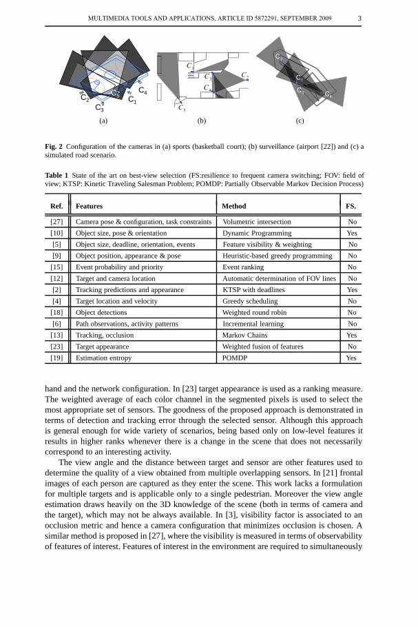
Fig. 2 Configuration of the cameras in (a) sports (basketball court); (b) surveillance (airport [22]) and (c) asimulated road scenario.

Table 1 State of the art on best-view selection (FS:resilience to frequent camera switching; FOV: field ofview; KTSP: Kinetic Traveling Salesman Problem; POMDP: Partially Observable Markov Decision Process)

Ref. Features Method FS.

[27] Camera pose & configuration, task constraints Volumetric intersection No

[10] Object size, pose & orientation Dynamic Programming Yes

[5] Object size, deadline, orientation, events Feature visibility & weighting No

[9] Object position, appearance & pose Heuristic-based greedy programming No

[15] Event probability and priority Event ranking No

[12] Target and camera location Automatic determination of FOV lines No

[2] Tracking predictions and appearance KTSP with deadlines Yes

[4] Target location and velocity Greedy scheduling No

[18] Object detections Weighted round robin No

[6] Path observations, activity patterns Incremental learning No

[13] Tracking, occlusion Markov Chains Yes

[23] Target appearance Weighted fusion of features No

[19] Estimation entropy POMDP Yes

hand and the network configuration. In [23] target appearance is used as a ranking measure.The weighted average of each color channel in the segmented pixels is used to select themost appropriate set of sensors. The goodness of the proposed approach is demonstrated interms of detection and tracking error through the selected sensor. Although this approachis general enough for wide variety of scenarios, being based only on low-level features itresults in higher ranks whenever there is a change in the scene that does not necessarilycorrespond to an interesting activity.

The view angle and the distance between target and sensor are other features used todetermine the quality of a view obtained from multiple overlapping sensors. In [21] frontalimages of each person are captured as they enter the scene. This work lacks a formulationfor multiple targets and is applicable only to a single pedestrian. Moreover the view angleestimation draws heavily on the 3D knowledge of the scene (both in terms of camera andthe target), which may not be always available. In [3], visibility factor is associated to anocclusion metric and hence a camera configuration that minimizes occlusion is chosen. Asimilar method is proposed in [27], where the visibility is measured in terms of observabilityof features of interest. Features of interest in the environment are required to simultaneously


4

be visible, inside the field of view, in focus, and magnified as per the specification of thetask at hand. Features extracted from the track information are fused to obtain a global scoreto mark regions as interesting on the basis of the quality of view.

In [7] the rank for each sensor is estimated as a weighted sum of individual featuresof each target. The combination of features (blob area, detection of face, its size and thedirection of motion of the target) is used to rank individual object features. Since this ap-proach does not incorporate high-level scene analysis (e.g., event detection), it is very likelythat the highest rank may be given to the sensor with the largest number of targets, whereassensors with fewer targets but containing interesting or abnormal behaviors may be ignored.Similarly the problem of content ranking is considered in [5] as an observation on multiplefeatures. Ranking is performed on the basis of the features and events associated to eachobject. The overall approach in this work is deadline driven and based on a constant direc-tion motion model. The work in [15] uses event information as a cue to select the best viewwhere the event recognition probability and the information about its importance are usedas selection criterion.

In [16] a dual camera system is proposed for indoor scenarios with walking people. Tar-gets are repeatedly zoomed in to acquire facial images using a supervised learning approachdriven by skin, motion and detectability of features. Priors such as size (height) and themotion path of the target are set to narrow the choice in selection of targets in the scene.However this work lacks a formulation for target scheduling and its performance degradesin crowded scenes. In [2, 18], target features such as gaze direction and motion dynamicsare used to compute the minimum time that the target will remain in the monitored area(deadline). This deadline can be used to assign weights to active cameras in order to decidewhich sensor can attend to the target with minimum adjustment cost [18].

In [29] the occupancy map of the objects is constructed and used as shape approxima-tion. Several features are then extracted from the occupancy map (distance covered, speed,direction, distance from the camera center, visibility and face visibility). The construction ofthe occupancy map reduces the amount of noise due to spurious detections. A similar voxelrepresentation is used for different body parts in [9] to determine pose of the target in orderto obtain its probability of visibility.

2.2 Camera selection

Camera selection takes into account physical constraints such as the scheduling interval,orientation speed (in case of an active camera) and location of sensors in the network. In [2]Time Dependent Orienteering (TDO), target motion, position, target birth and deadline areused to trigger a PTZ camera that capture targets in the scene. To minimize the number ofswitches a scheduling interval is used. The cost of the system is associated to the numberof targets not captured. The scheduling strategy used is Kinetic Traveling Salesperson Prob-lem with deadlines. A schedule to observe targets is chosen which minimizes the path costin term of TDO. This work does not consider target occlusions and does not provide anyformulation for the prediction of the best time intervals to capture images. In [10] a costfunction is proposed that depends on the view quality measures using features such as ob-ject size, pose and orientation. This cost function also includes a penalizing factor to avoidfrequent switches.

In [31] a single person is tracked by an active camera and when there is more then oneperson in the view of the static camera, the active camera focuses on the closest target. Theperformance of the system degrades in case of crowded scenes as the camera switches from


5

target to target. In [17], a surveillance system is proposed, comprising of passive cameraswith wide field-of-view and an active camera which automatically captures and labels high-resolution videos of pedestrians. A Weighted Round Robin technique is used for schedulingeach target that enters the monitored area. The approach is scalable both in terms of numberof cameras and targets.

The work in [4] uses greedy scheduling policies to observe people where targets aretreated as network packets and a routing approach based on techniques such as First ComeFirst Served (FCFS), Earliest Deadline First (EDF) and Current Minloss Throughput Opti-mal (CMTO). However these approaches do not include the transition cost for the camerathat is associated with target swaps. A system for automatically acquiring high-resolutionimages by steering a pan-tilt-zoom (PTZ) camera is described in [20]. The system uses cali-brated master cameras to steer slave cameras. However, in case of multiple targets, the slavePTZ cameras focuses on the target which was detected first in the scene and then basedon the arrival time of the targets subsequent scheduling of targets is done. In [8] a ceilingmounted omni-directional camera provides input for a PTZ camera mounted at head heightto capture facial images of the targets moving in the scene. No formulation is provided totackle lost objects and for cluttered scenes there is significat degradation in the performanceof the system. In addition there needs to be accurate calibration between the master andslave cameras.

The work in [1] concentrates on active tracking: a simple behavior (a policy) with afinite state machine is defined in order to give some form of continuity when the currentlytracked target is changed. Authors in [19] propose the use of Partially Observable MarkovDecision Processes (POMDP) to estimate the state of the target at any time and select acamera configuration so that estimation error in detecting the state of the target is minimized.Scheduling interval is used to observe targets for a duration of time. However they do nottake into account target interactions with the environment and no formulation is providedfor multiple targets.

3 Problem formulation

Let a set of N cameras C = {C1, . . . ,CN}, with camera Ci at time t observe a set of Ji(t)targets Oi(t) = {Oi1(t), . . . ,OiJi(t)}. The problem of view selection consists in deciding thebest view C(t) at any time t such that features of interest are visible [27] and/or maxi-mized [3]. Such a view is likely to contain information about the scene which is of mostinterest, given the site contextual information and camera network information. Let us de-fine the set of features observed by each camera Ci as ψi(t). Based on these features, ascore ρi(t) = f (ϑi,ψi(t)) is assigned to it, where ϑi is a set of parameters for camera Ci

that encode the contextual information regarding the site. This score helps selecting cameraC(t) ∈C at each time instant t. In order to avoid frequent switches and generate a pleasantview, let us consider the cameras as a set of states of the system. Then the problem is to findthe most likely state based on a observations vector ρ(t) = (ρ1(t), . . . ,ρN(t)), where ρi(t) isthe score for camera Ci at time t.

The problem of camera selection can thus be regarded as a three-tier system (Fig. 1). Inthe first stage, the extraction of a feature set ψi(t) at time t for each object in each cameraCi, ∀ i = 1, . . . ,N is performed. In the second stage, the features are used to generate acamera score ρ(t). In the final stage, a selection mechanism is constructed as a function oftime t and the rank ρ(t) to select C(t).


6

(a) (b) (c)

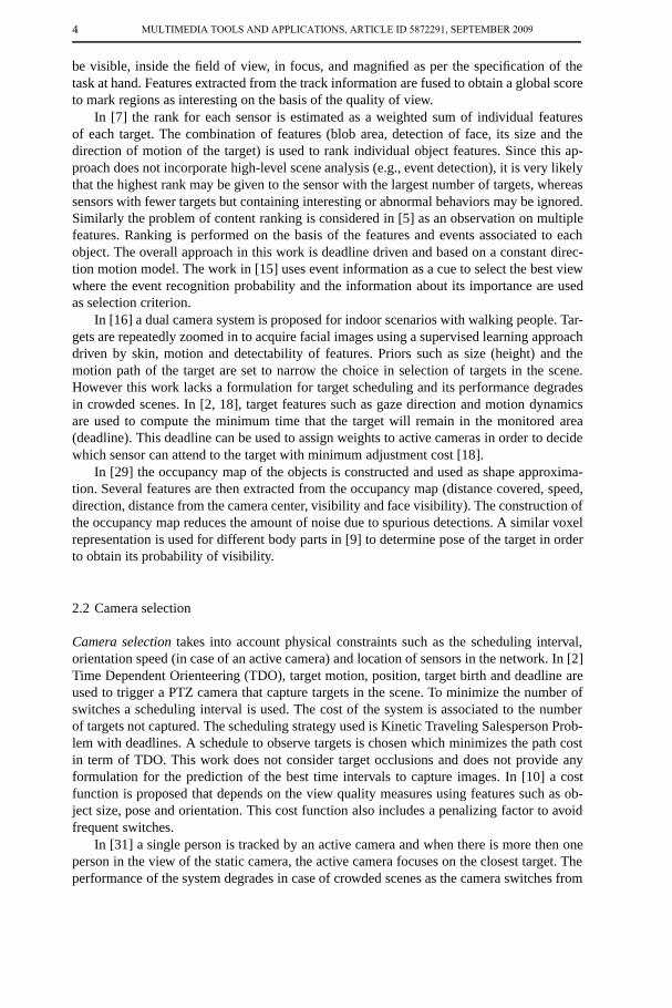
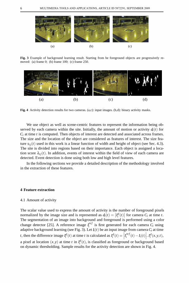
Fig. 3 Example of background learning result. Starting from he foreground objects are progressively re-moved: (a) frame 0; (b) frame 100; (c) frame 250.

(a) (b) (c) (d)

Fig. 4 Activity detection results for two cameras. (a,c): input images. (b,d): binary activity masks.

We use object as well as scene-centric features to represent the information being ob-served by each camera within the site. Initially, the amount of motion or activity di(t) forCi at time t is computed. Then objects of interest are detected and associated across frames.The size and the location of the object are considered as features of interest. The size fea-ture si j(t) used in this work is a linear function of width and height of object (see Sec. 4.3).The site is divided into regions based on their importance. Each object is assigned a loca-tion score λi j(t). In addition, events of interest within the field of view of each camera aredetected. Event detection is done using both low and high level features.

In the following sections we provide a detailed description of the methodology involvedin the extraction of these features.

4 Feature extraction

4.1 Amount of activity

The scalar value used to express the amount of activity is the number of foreground pixelsnormalized by the image size and is represented as di(t) =

∣∣Idi (t)

∣∣ for camera Ci at time t.The segmentation of an image into background and foreground is performed using a colorchange detector [25]. A reference image Ire f

i is first generated for each camera Ci usingadaptive background learning (see Fig. 3). Let Ii(t) be an input image from camera Ci at time

t, then the difference image Idi (t) at time t is calculated as Id

i (t) =∣∣∣Ire f

i (t)− Ii(t)∣∣∣. Id

i (x,y, t),

a pixel at location (x,y) at time t in Idi (t), is classified as foreground or background based

on dynamic thresholding. Sample results for the activity detection are shown in Fig. 4.


7

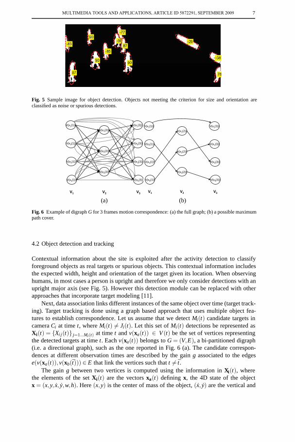
Fig. 5 Sample image for object detection. Objects not meeting the criterion for size and orientation areclassified as noise or spurious detections.

V(x1(1))

V(x2(1))

V(x3(1))

V(x4(1))

V(x1(2))

V(x2(2))

V(x3(2))

V(x1(3))

V(x2(3))

V(x3(3))

V(x4(3))

V1 V2 V3

V(x1(1))

V(x2(1))

V(x3(1))

V(x4(1))

V(x1(2))

V(x2(2))

V(x3(2))

V(x1(3))

V(x2(3))

V(x3(3))

V(x4(3))

V1 V2 V3

(a) (b)

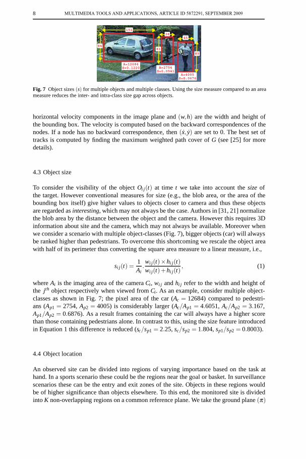
Fig. 6 Example of digraph G for 3 frames motion correspondence: (a) the full graph; (b) a possible maximumpath cover.

4.2 Object detection and tracking

Contextual information about the site is exploited after the activity detection to classifyforeground objects as real targets or spurious objects. This contextual information includesthe expected width, height and orientation of the target given its location. When observinghumans, in most cases a person is upright and therefore we only consider detections with anupright major axis (see Fig. 5). However this detection module can be replaced with otherapproaches that incorporate target modeling [11].

Next, data association links different instances of the same object over time (target track-ing). Target tracking is done using a graph based approach that uses multiple object fea-tures to establish correspondence. Let us assume that we detect Mi(t) candidate targets incamera Ci at time t, where Mi(t) �= Ji(t). Let this set of Mi(t) detections be represented asXi(t) = {Xi j(t)} j=1...Mi(t) at time t and v(xa(t)) ∈ V (t) be the set of vertices representingthe detected targets at time t. Each v(xa(t)) belongs to G = (V,E), a bi-partitioned digraph(i.e. a directional graph), such as the one reported in Fig. 6 (a). The candidate correspon-dences at different observation times are described by the gain g associated to the edgese(v(xa(t)),v(xb(t))) ∈ E that link the vertices such that t �= t .

The gain g between two vertices is computed using the information in Xi(t), wherethe elements of the set Xi(t) are the vectors xa(t) defining x, the 4D state of the objectx = (x,y, x, y,w,h). Here (x,y) is the center of mass of the object, (x, y) are the vertical and


8

34

8184

89

151

45

A=12684S=0.1220 A=2754

S=0.0541A=4005S=0.0676

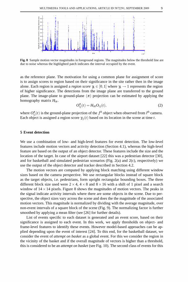
Fig. 7 Object sizes (s) for multiple objects and multiple classes. Using the size measure compared to an areameasure reduces the inter- and intra-class size gap across objects.

horizontal velocity components in the image plane and (w,h) are the width and height ofthe bounding box. The velocity is computed based on the backward correspondences of thenodes. If a node has no backward correspondence, then (x, y) are set to 0. The best set oftracks is computed by finding the maximum weighted path cover of G (see [25] for moredetails).

4.3 Object size

To consider the visibility of the object Oi j(t) at time t we take into account the size ofthe target. However conventional measures for size (e.g., the blob area, or the area of thebounding box itself) give higher values to objects closer to camera and thus these objectsare regarded as interesting, which may not always be the case. Authors in [31, 21] normalizethe blob area by the distance between the object and the camera. However this requires 3Dinformation about site and the camera, which may not always be available. Moreover whenwe consider a scenario with multiple object-classes (Fig. 7), bigger objects (car) will alwaysbe ranked higher than pedestrians. To overcome this shortcoming we rescale the object areawith half of its perimeter thus converting the square area measure to a linear measure, i.e.,

si j(t) =1Ai

.wi j(t)×hi j(t)wi j(t)+hi j(t)

, (1)

where Ai is the imaging area of the camera Ci, wi j and hi j refer to the width and height ofthe jth object respectively when viewed from Ci. As an example, consider multiple object-classes as shown in Fig. 7; the pixel area of the car (Ac = 12684) compared to pedestri-ans (Ap1 = 2754, Ap2 = 4005) is considerably larger (Ac/Ap1 = 4.6051, Ac/Ap2 = 3.167,Ap1/Ap2 = 0.6876). As a result frames containing the car will always have a higher scorethan those containing pedestrians alone. In contrast to this, using the size feature introducedin Equation 1 this difference is reduced (sc/sp1 = 2.25, sc/sp2 = 1.804, sp1/sp2 = 0.8003).

4.4 Object location

An observed site can be divided into regions of varying importance based on the task athand. In a sports scenario these could be the regions near the goal or basket. In surveillancescenarios these can be the entry and exit zones of the site. Objects in these regions wouldbe of higher significance than objects elsewhere. To this end, the monitored site is dividedinto K non-overlapping regions on a common reference plane. We take the ground plane (π)


9

0 1 2 3 4 5 6 7 8 9

x 104

0

0.1

0.2

0.3

0.4

0.5

0.6

0.7

0.8

0.9

1

time

Mag

nitu

de o

f mot

ion

vect

ors

x ch

ange

det

ectio

n ar

ea

Fig. 8 Sample motion vector magnitudes in foreground regions. The magnitudes below the threshold line aredue to noise whereas the highlighted patch indicates the interval occupied by the event.

as the reference plane. The motivation for using a common plane for assignment of scoreis to assign scores to region based on their significance in the site rather then in the imagealone. Each region is assigned a region score γk ∈ [0,1] where γk → 1 represents the regionof higher significance. The detections from the image plane are transferred to the groundplane. The image-plane to ground-plane (π) projection can be estimated by applying thehomography matrix Hiπ .

Oπi j(t) = HiπOi j(t), (2)

where Oπi j(t) is the ground-plane projection of the jth object when observed from ith camera.

Each object is assigned a region score γi j(t) based on its location in the scene at time t.

5 Event detection

We use a combination of low- and high-level features for event detection. The low-levelfeatures include motion vectors and activity detection (Section 4.1), whereas the high-levelfeature are based on the output of an object detector. These features include the size and thelocation of the target. In case of the airport dataset [22] this was a pedestrian detector [30],and for basketball and simulated pedestrian scenarios (Fig. 2(a) and 2(c), respectively) weuse the output of the object detector and tracker described in Section 4.2.

The motion vectors are computed by applying block matching using different windowsizes based on the camera perspective. We use rectangular blocks instead of square blockas the target objects, i.e. pedestrians, form upright rectangular bounding boxes. The threedifferent block size used were 2× 4, 4× 8 and 8× 16 with a shift of 1 pixel and a searchwindow of 14×14 pixels. Figure 8 shows the magnitudes of motion vectors. The peaks inthe signal indicate activity intervals where there are some objects in the scene. Due to per-spective, the object sizes vary across the scene and does the the magnitude of the associatedmotion vectors. This magnitude is normalized by dividing with the average magnitude, overnon-event intervals of a square block of the scene (Fig. 9). The normalizing factor is furthersmoothed by applying a mean filter (see [26] for further details).

List of events specific to each dataset is generated and an event score, based on theirsignificance is assigned to each event. In this work, we apply thresholds on object- andframe-level features to identify these events. However model-based approaches can be ap-plied depending upon the event of interest [24]. To this end, for the basketball dataset, weconsider the event of attempt on basket as a global event. For this we consider the region inthe vicinity of the basket and if the overall magnitude of vectors is higher than a threshold,this is considered to be an attempt on basket (see Fig. 10). The second class of events for this


10

0

10

20

30

40

50

010

2030

40

0

5

10

15

20

x

y

aver

age

spee

d

Fig. 9 Sample normalization factor to compensate for changes in perspective due to object size, computedfor each 16×16 region of the image.

Fig. 10 An example frame for attempt on basket event.

data set is the high activity event. This event is directly related to the amount of motion vec-tors in the scene and the amount of activity di(t) associated to the frame. The event consid-ered for the pedestrian dataset was the event of an object being on the road (marked by greenlines for visualization in Fig. 13) for a duration longer then β time instances (pedestrian-on-road event). For this we consider the location score γi j(t) associated to each object Oi j

being observed from camera Ci at time t. In these set of experiments we use a value of β ≥ 15frames. In the airport surveillance dataset we performed the detection of three events namelyperson runs (total magnitude of motion vectors normalized with average magnitude of mo-tion vectors within a region), elevator no entry (when an object does not enter the elevatorwith elevator door open) and opposing flow (a person walking in a direction opposite to theallowed direction).

Assume that there are Ls possible events which can happen for a multi-camera setupand this set is represented as Γ = {λ1, . . . ,λLs}. Based on the importance of each event, itis assigned a score θ l |l=1,...,Ls . If a set λ l

i (t)l=1,...,Li ∈ Γ of Li events are detected in cameraCi at time t, the total event score Θi(t) for each camera at time t is given as Θi(t) = ∑Li

l θ li ,

where θ li for l = 1, . . . ,Li is the list of event scores seen by camera Ci at time t.


11

contextualinformation

i

)(tijklocation

)...1|( Kkk

iC

objectdetection& tracking )(tsij

objectscore

)(tk

size score

locationscore

)(,...,1|)( tJjt iijiA

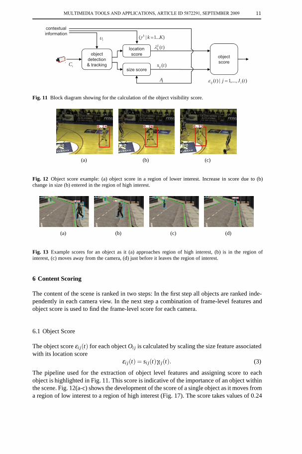
Fig. 11 Block diagram showing for the calculation of the object visibility score.

(a) (b) (c)

Fig. 12 Object score example: (a) object score in a region of lower interest. Increase in score due to (b)change in size (b) entered in the region of high interest.

(a) (b) (c) (d)

Fig. 13 Example scores for an object as it (a) approaches region of high interest, (b) is in the region ofinterest, (c) moves away from the camera, (d) just before it leaves the region of interest.

6 Content Scoring

The content of the scene is ranked in two steps: In the first step all objects are ranked inde-pendently in each camera view. In the next step a combination of frame-level features andobject score is used to find the frame-level score for each camera.

6.1 Object Score

The object score εi j(t) for each object Oi j is calculated by scaling the size feature associatedwith its location score

εi j(t) = si j(t)γi j(t). (3)

The pipeline used for the extraction of object level features and assigning score to eachobject is highlighted in Fig. 11. This score is indicative of the importance of an object withinthe scene. Fig. 12(a-c) shows the development of the score of a single object as it moves froma region of low interest to a region of high interest (Fig. 17). The score takes values of 0.24


12

0 200 400 600 800 1000 12001

2

3

4

5

frames

sele

cted

cam

era

id

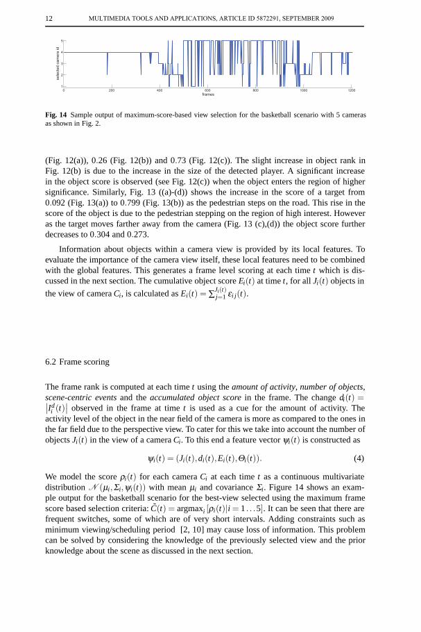
Fig. 14 Sample output of maximum-score-based view selection for the basketball scenario with 5 camerasas shown in Fig. 2.

(Fig. 12(a)), 0.26 (Fig. 12(b)) and 0.73 (Fig. 12(c)). The slight increase in object rank inFig. 12(b) is due to the increase in the size of the detected player. A significant increasein the object score is observed (see Fig. 12(c)) when the object enters the region of highersignificance. Similarly, Fig. 13 ((a)-(d)) shows the increase in the score of a target from0.092 (Fig. 13(a)) to 0.799 (Fig. 13(b)) as the pedestrian steps on the road. This rise in thescore of the object is due to the pedestrian stepping on the region of high interest. Howeveras the target moves farther away from the camera (Fig. 13 (c),(d)) the object score furtherdecreases to 0.304 and 0.273.

Information about objects within a camera view is provided by its local features. Toevaluate the importance of the camera view itself, these local features need to be combinedwith the global features. This generates a frame level scoring at each time t which is dis-cussed in the next section. The cumulative object score Ei(t) at time t, for all Ji(t) objects in

the view of camera Ci, is calculated as Ei(t) = ∑Ji(t)j=1 εi j(t).

6.2 Frame scoring

The frame rank is computed at each time t using the amount of activity, number of objects,scene-centric events and the accumulated object score in the frame. The change di(t) =∣∣Id

i (t)∣∣ observed in the frame at time t is used as a cue for the amount of activity. The

activity level of the object in the near field of the camera is more as compared to the ones inthe far field due to the perspective view. To cater for this we take into account the number ofobjects Ji(t) in the view of a camera Ci. To this end a feature vector ψi(t) is constructed as

ψi(t) = (Ji(t),di(t),Ei(t),Θi(t)). (4)

We model the score ρi(t) for each camera Ci at each time t as a continuous multivariatedistribution N (μi,Σi,ψi(t)) with mean μi and covariance Σi. Figure 14 shows an exam-ple output for the basketball scenario for the best-view selected using the maximum framescore based selection criteria: C(t) = argmaxi [ρi(t)|i = 1 . . .5]. It can be seen that there arefrequent switches, some of which are of very short intervals. Adding constraints such asminimum viewing/scheduling period [2, 10] may cause loss of information. This problemcan be solved by considering the knowledge of the previously selected view and the priorknowledge about the scene as discussed in the next section.


13

C1P(C3|C1)P(C1) P(C5|C1)P(C1)

C2P(C2|C1)P(C1) P(C2|C1)P(C1)

C3

C2

P(C4|C2)P(C2| (C2)) P(C5|C2)P(C2| (C3))

C CP(C4|C3)P(C3| (C3)) P(C5|C3)P(C3| (C3))

C4 C5

(a)

Ci(1) Ci(2) Ci(3)Ci(1) Ci(2) Ci(3)

i(1) i(2) i(3)

(b)

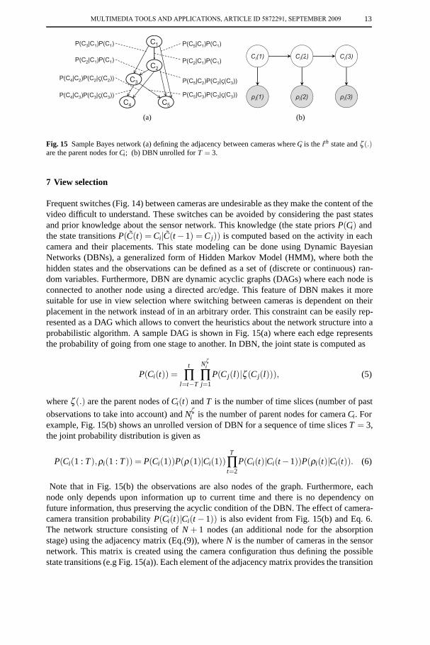
Fig. 15 Sample Bayes network (a) defining the adjacency between cameras where Ci is the ith state and ζ (.)are the parent nodes for Ci; (b) DBN unrolled for T = 3.

7 View selection

Frequent switches (Fig. 14) between cameras are undesirable as they make the content of thevideo difficult to understand. These switches can be avoided by considering the past statesand prior knowledge about the sensor network. This knowledge (the state priors P(Ci) andthe state transitions P(C(t) = Ci|C(t −1) = Cj)) is computed based on the activity in eachcamera and their placements. This state modeling can be done using Dynamic BayesianNetworks (DBNs), a generalized form of Hidden Markov Model (HMM), where both thehidden states and the observations can be defined as a set of (discrete or continuous) ran-dom variables. Furthermore, DBN are dynamic acyclic graphs (DAGs) where each node isconnected to another node using a directed arc/edge. This feature of DBN makes it moresuitable for use in view selection where switching between cameras is dependent on theirplacement in the network instead of in an arbitrary order. This constraint can be easily rep-resented as a DAG which allows to convert the heuristics about the network structure into aprobabilistic algorithm. A sample DAG is shown in Fig. 15(a) where each edge representsthe probability of going from one stage to another. In DBN, the joint state is computed as

P(Ci(t)) =t

∏l=t−T

Nζi

∏j=1

P(Cj(l)|ζ (Cj(l))), (5)

where ζ (.) are the parent nodes of Ci(t) and T is the number of time slices (number of past

observations to take into account) and Nζi is the number of parent nodes for camera Ci. For

example, Fig. 15(b) shows an unrolled version of DBN for a sequence of time slices T = 3,the joint probability distribution is given as

P(Ci(1 : T),ρi(1 : T )) = P(Ci(1))P(ρ(1)|Ci(1))T

∏t=2

P(Ci(t)|Ci(t−1))P(ρi(t)|Ci(t)). (6)

Note that in Fig. 15(b) the observations are also nodes of the graph. Furthermore, eachnode only depends upon information up to current time and there is no dependency onfuture information, thus preserving the acyclic condition of the DBN. The effect of camera-camera transition probability P(Ci(t)|Ci(t − 1)) is also evident from Fig. 15(b) and Eq. 6.The network structure consisting of N + 1 nodes (an additional node for the absorptionstage) using the adjacency matrix (Eq.(9)), where N is the number of cameras in the sensornetwork. This matrix is created using the camera configuration thus defining the possiblestate transitions (e.g Fig. 15(a)). Each element of the adjacency matrix provides the transition


14

probability of selecting a view given the current view. Formally, the probability of observingstate Ci given the current state is Cj can be computed as

P(Ci(t)|Cj(t −1)) = P(Ci(t)|Cj(t−1))P(Ci(t)|ζ (Cj(t −1))). (7)

In this computation we assume the model to be first order Markov and the transition andobservation functions are time-invariant i.e. P(Ci(t)|Cj(1 : t −1)) = P(Ci(t)|Cj(t −1)). Tofacilitate transitions after the system is in the absorbing state, a auxiliary node is introducedwhich allows transition to the parent nodes. The scores ρi for each camera Ci are used asobservation for the Bayesian network. The observation is an N-dimensional feature vectordefined as ρ(t) = {ρ1(t), · · · ,ρN(t)}. The states are modeled using binomial distribution.The choice of binomial distribution is because in this distribution each trial results in exactlyone of some fixed finite number k of possible outcomes, with probabilities (p1, · · · , pk) suchthat ∑k

i=1 pi = 1, and there are ntr independent trials. The parameter learning for each node isbased on Expectation Maximization [14] algorithm. The training is performed for each stateup to n iterations or until the change in log likelihood is less then a threshold η = 10−100.The likelihood for each state is calculated by applying marginalization. The final cameraselection C(t) is then computed as

C(t) = argmaxi

[ϒ (ρi(t −T : t)|P(Ci(t)))P(Ci(t))] , (8)

where ϒ (.) is assumed to be Gaussian and P(Ci) is the prior on the state.

8 Results

To evaluate the performance of the proposed approach we show two different types of ex-periments. The first set of experiments regards the content scoring and camera selection.The second experiment focuses on the evaluation of the system in terms of selection ofthe best-view while minimizing the number of view switches. In both sets of experimentswe demonstrate the effectiveness of the proposed approach by comparing it with manuallygenerated ground-truth. The ground-truth was done manually by 11 non-professional users.Each user was asked to select a camera view at each time instant. Then the view selected bymajority of the users was chosen as the best-view at that time instant.

8.1 Experimental setup

We demonstrate the performance of the proposed approach on three scenarios, namely abasketball game, an indoor airport surveillance and an outdoor scene. The basketball game(Fig. 2(a)) is monitored by 5 cameras with partially overlapping fields of view. The data con-sists of a total of 17960 frames, out of which 500 were used for training the DBN and theremaining were used for testing. Contextual information is composed of the expected sizeand orientation of the players in each camera view. The regions of the video outside the fieldare not considered, and any features of interest observed in these regions are ignored. Thecamera network configuration is encoded in the form of Bayes net as shown in Fig. 15(a).The indoor airport surveillance dataset was also acquired using 5 partially overlapping cam-eras (Fig. 2(b)). The section of data on which we demonstrate the proposed approach con-tains 180006 frames for each camera, out of which 1000 were used for training the DBNand remaining for testing the algorithm. Contextual information in this case is composed of


15

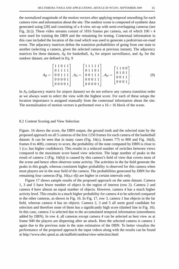
the normalized magnitude of the motion vectors after applying temporal smoothing for eachcamera view and information about the site. The outdoor scene is composed of synthetic datagenerated using [28] and consisting of a 4-view set-up with semi-overlapping cameras (seeFig. 2(c)). These video streams consist of 1816 frames per camera, out of which 100× 4were used for training the DBN and the remaining for testing. Contextual information inthis case included the location of the road which was used to generate a pedestrian-on-roadevent. The adjacency matrices define the transition probabilities of going from one state toanother (selecting a camera, given the selected camera at previous instant). The adjacencymatrices for these datasets, AB for basketball, AA for airport surveillance, and AH for theoutdoor dataset, are defined in Eq. 9

AB =

⎡⎢⎢⎢⎢⎣

1 1 0 1 10 1 1 1 10 0 1 1 10 0 0 0 10 0 0 0 1

⎤⎥⎥⎥⎥⎦

,AA =

⎡⎢⎢⎢⎢⎣

1 1 1 1 10 1 1 0 10 0 1 1 10 0 0 1 10 0 0 0 1

⎤⎥⎥⎥⎥⎦

,AH =

⎡⎢⎢⎣

1 1 0 00 1 0 10 0 1 10 0 0 1

⎤⎥⎥⎦ . (9)

In AA (adjacency matrix for airport dataset) we do not enforce any camera transition orderas we always want to select the view with the highest score. For each of these setups thelocation importance is assigned manually from the contextual information about the site.The normalization of motion vectors is performed over a 16×16 block of the scene.

8.2 Content Scoring and View Selection

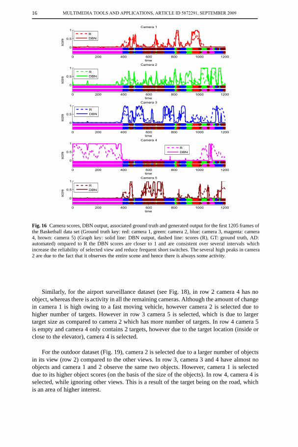
Figure. 16 shows the score, the DBN output, the ground truth and the selected state by theproposed approach on all 5 cameras of the first 1250 frames for each camera of the basketballdataset. It can be seen that in many cases (Fig. 16(c), frames 775 to 800 and Fig. 16(d),frames 0 to 400), contrary to score, the probability of the state computed by DBN is close to1 (i.e. has higher confidence). This results in a reduced number of switches between viewscompared to the maximum score based view selection. The large number of peaks in theresult of camera 2 (Fig. 16(b)) is caused by this camera’s field of view that covers most ofthe scene and hence often observes some activity. The activities in the far field generate thepeaks in this graph, whereas consistent higher probability is observed for this camera whenmost players are in the near field of the camera. The probabilities generated by DBN for theremaining four cameras (Fig. 16(a,c-d)) are higher in certain intervals only.

Figure 17 shows sample results of the proposed approach on the same dataset. Camera1, 3 and 5 have fewer number of object in the region of interest (row 2). Camera 2 andcamera 4 have almost an equal number of objects. However, camera 4 has a much higheractivity level. This results in a much higher probability for camera 4 to be selected comparedto the other cameras, as shown in Fig. 16. In Fig. 17, row 3, camera 1 has objects in the farfield, whereas camera 4 has no objects. Camera 2, 3 and 5 all seem good candidate forselection and therefore none of them has a significantly high score (dashed line in Fig. 16).In this case, camera 3 is selected due to the accumulated temporal information (smoothnessadded by DBN). In row 4, all cameras except camera 4 can be selected as best view as atframe 940 the players are dispersing after an attack. Here the selected camera is camera 1again due to the previous state in the state estimation of the DBN. To better visualize theperformance of the proposed approach the input videos along with the results can be foundat http://www.elec.qmul.ac.uk/staffinfo/andrea/view-selection.html


16

0 200 400 600 800 1000 1200

0

0.5

1

timesc

ore

Camera 1

RDBN

0 200 400 600 800 1000 1200

0

0.5

1

time

scor

eCamera 2

RDBN

0 200 400 600 800 1000 1200

0

0.5

1

time

scor

e

Camera 3

RDBN

0 200 400 600 800 1000 1200

0

0.5

1

time

scor

e

Camera 4

RDBN

0 200 400 600 800 1000 1200

0

0.5

1

time

scor

e

Camera 5

RDBN

Fig. 16 Camera scores, DBN output, associated ground truth and generated output for the first 1205 frames ofthe Basketball data set (Ground truth key: red: camera 1, green: camera 2, blue: camera 3, magenta: camera4, brown: camera 5) (Graph key: solid line: DBN output, dashed line: scores (R), GT: ground truth, AD:automated) ompared to R the DBN scores are closer to 1 and are consistent over several intervals whichincrease the reliability of selected view and reduce frequent short switches. The several high peaks in camera2 are due to the fact that it observes the entire scene and hence there is always some activity.

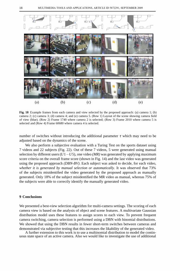
Similarly, for the airport surveillance dataset (see Fig. 18), in row 2 camera 4 has noobject, whereas there is activity in all the remaining cameras. Although the amount of changein camera 1 is high owing to a fast moving vehicle, however camera 2 is selected due tohigher number of targets. However in row 3 camera 5 is selected, which is due to largertarget size as compared to camera 2 which has more number of targets. In row 4 camera 5is empty and camera 4 only contains 2 targets, however due to the target location (inside orclose to the elevator), camera 4 is selected.

For the outdoor dataset (Fig. 19), camera 2 is selected due to a larger number of objectsin its view (row 2) compared to the other views. In row 3, camera 3 and 4 have almost noobjects and camera 1 and 2 observe the same two objects. However, camera 1 is selecteddue to its higher object scores (on the basis of the size of the objects). In row 4, camera 4 isselected, while ignoring other views. This is a result of the target being on the road, whichis an area of higher interest.


17

(a) (b) (c) (d) (e)

Fig. 17 Example frames from each camera and view selected by the proposed approach: (a) camera 1; (b)camera 2; (c) camera 3; (d) camera 4; and (e) camera 5. (Row 1) Layout of the scene showing camera fieldof view (blue) and regions of high interest (green). (Row 2) Frame 255 where camera 4 is selected; (Row 3)Frame 540 where camera 3 is selected and (Row 4) Frame 940 where camera 1 is selected.

8.3 Complexity

To compute the computational cost of the entire algorithm, we consider the three stagesoutlined in Fig. 1. Each stage further contains sub-processes as highlighted in Fig. 20. Thestated percentage average times were calculated on an Intel 3.2 GHz Pentium dual core usingnon-optimized implementation. The detection and tracking was done using visual C++ andremaining modules were implemented using Matlab. It can be seen in Fig. 20 that the detec-tion and tracking module contributes to 61.53% of the total computational cost. The frameranking (5.95%) and the view selection (11.22%) on the other hand, takes only 17.15% ofthe total time. This shows that the bulk of the time (82.85%) is consumed in object detec-tion and tracking and feature extraction (stage one of Fig. 1). This indicates that given anefficient implementation for detection, tracking and feature extraction the proposed viewselection can be easily performed in short time duration.

8.4 Evaluation

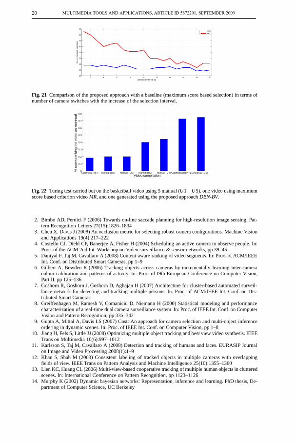
To evaluate the effectiveness of the smoothing introduced by the proposed approach (DBN-BV) we compare it with a maximum score (MR) based approach. In this approach we in-troduce the selection interval τ and the decision is taken at the beginning of each selectioninterval. This results in reducing the number of switches as the change of view is only al-lowed after τ frames. Figure 21 shows the result where the number of switches reducesfrom 53 to 26 as τ increases from 1 to 20 when using MR. In case of DBN, the number ofswitches decreases from 24 to 20 only. This shows that by using DBN we can reduce the


18

(a) (b) (c) (d) (e)

Fig. 18 Example frames from each camera and view selected by the proposed approach: (a) camera 1; (b)camera 2; (c) camera 3; (d) camera 4; and (e) camera 5. (Row 1) Layout of the scene showing camera fieldof view (blue). (Row 2) Frame 1740 where camera 2 is selected; (Row 3) Frame 2010 where camera 5 isselected and (Row 4) Frame 60680 where camera 4 is selected.

number of switches without introducing the additional parameter τ which may need to beadjusted based on the dynamics of the scene.

We also perform a subjective evaluation with a Turing Test on the sports dataset using7 videos and 22 subjects (Fig. 22). Out of these 7 videos, 5 were generated using manualselection by different users (U1−U5), one video (MR) was generated by applying maximumscore criteria on the overall frame score (shown in Fig. 14) and the last video was generatedusing the proposed approach (DBN-BV). Each subject was asked to decide, for each video,whether it is generated by manual selection or automatically. It was observed that 73%of the subjects misidentified the video generated by the proposed approach as manuallygenerated. Only 18% of the subject misidentified the MR video as manual, whereas 75% ofthe subjects were able to correctly identify the manually generated video.

9 Conclusions

We presented a best-view selection algorithm for multi-camera settings. The scoring of eachcamera view is based on the analysis of object and scene features. A multivariate Gaussiandistribution model uses these features to assign scores to each view. To prevent frequentcamera switching, camera selection is performed using a DBN with binomial distributions.We showed that using the DBN results in fewer short-term switches between cameras anddemonstrated via subjective testing that this increases the likability of the generated video.

A further extension to this work is to use a multinomial distribution to model the contin-uous state space of an active camera. Also we would like to investigate the use of additional


19

(a) (b) (c) (d)

Fig. 19 Example frames from each camera and view selected by the proposed approach: (a) camera 1; (b)camera 2; (c) camera 3 and (e) camera 4. (Row 1) Layout of the scene showing camera field of view (blue).(Row 2) Frame 184 where camera 2 is selected; (Row 3) Frame 476 where camera 1 is selected and (Row 4)Frame 1627 where camera 4 is selected.

61.53%

19.11%

2.21%5.93%

11.22%

Object detection & tracking

Feature extraction

Event detection

Frame score computation

61.53%

19.11%

2.21%5.93%

11.22%

Object detection & tracking

Feature extraction

Event detection

Frame score computation

View selection

Fig. 20 Percentage average time for each module of the proposed approach.

features such as object tracking and motion models to enable the system to predict the nextbest view.

References

1. Batista J, Peixoto P, Araujo H (1998) Real-time active visual surveillance by integrating peripheral mo-tion detection with foveated tracking. In: Proc. of IEEE Workshop on Visual Surveillance, pp 18–25


20

2 4 6 8 10 12 14 16 18 2015

20

25

30

35

40

45

50

55

selection interval (τ)

No.

of c

amer

a sw

itche

s

DBNMR

Fig. 21 Comparison of the proposed approach with a baseline (maximum score based selection) in terms ofnumber of camera switches with the increase of the selection interval.

Automatic (MR) Manual (U3) Manual (U5) Manual (U2) Manual (U4)Automatic (DBN−BV)Manual (U1)0

0.1

0.2

0.3

0.4

0.5

0.6

0.7

0.8

Video compilation

% u

sers

ran

king

the

vide

o as

man

nual

Fig. 22 Turing test carried out on the basketball video using 5 manual (U1−U5), one video using maximumscore based criterion video MR, and one generated using the proposed approach DBN-BV.

2. Bimbo AD, Pernici F (2006) Towards on-line saccade planning for high-resolution image sensing. Pat-tern Recognition Letters 27(15):1826–1834

3. Chen X, Davis J (2008) An occlusion metric for selecting robust camera configurations. Machine Visionand Applications 19(4):217–222

4. Costello CJ, Diehl CP, Banerjee A, Fisher H (2004) Scheduling an active camera to observe people. In:Proc. of the ACM 2nd Int. Workshop on Video surveillance & sensor networks, pp 39–45

5. Daniyal F, Taj M, Cavallaro A (2008) Content-aware ranking of video segments. In: Proc. of ACM/IEEEInt. Conf. on Distributed Smart Cameras, pp 1–9

6. Gilbert A, Bowden R (2006) Tracking objects across cameras by incrementally learning inter-cameracolour calibration and patterns of activity. In: Proc. of I9th European Conference on Computer Vision,Part II, pp 125–136

7. Goshorn R, Goshorn J, Goshorn D, Aghajan H (2007) Architecture for cluster-based automated surveil-lance network for detecting and tracking multiple persons. In: Proc. of ACM/IEEE Int. Conf. on Dis-tributed Smart Cameras

8. Greiffenhagen M, Ramesh V, Comaniciu D, Niemann H (2000) Statistical modeling and performancecharacterization of a real-time dual camera surveillance system. In: Proc. of IEEE Int. Conf. on ComputerVision and Pattern Recognition, pp 335–342

9. Gupta A, Mittal A, Davis LS (2007) Cost: An approach for camera selection and multi-object inferenceordering in dynamic scenes. In: Proc. of IEEE Int. Conf. on Computer Vision, pp 1–8

10. Jiang H, Fels S, Little JJ (2008) Optimizing multiple object tracking and best view video synthesis. IEEETrans on Multimedia 10(6):997–1012

11. Karlsson S, Taj M, Cavallaro A (2008) Detection and tracking of humans and faces. EURASIP Journalon Image and Video Processing 2008(1):1–9

12. Khan S, Shah M (2003) Consistent labeling of tracked objects in multiple cameras with overlappingfields of view. IEEE Trans on Pattern Analysis and Machine Intelligence 25(10):1355–1360

13. Lien KC, Huang CL (2006) Multi-view-based cooperative tracking of multiple human objects in clutteredscenes. In: International Conference on Pattern Recognition, pp 1123–1126

14. Murphy K (2002) Dynamic bayesian networks: Representation, inference and learning. PhD thesis, De-partment of Computer Science, UC Berkeley


21

15. Park HS, Lim S, Min JK, Cho SB (2008) Optimal view selection and event retrieval in multi-cameraoffice environment. In: Proc. of IEEE Int. Conf. on Multisensor Fusion and Integration for IntelligentSystems, pp 106–110

16. Prince SJD, Elder JH, Hou Y, Sizinstev M (2005) Pre-attentive face detection for foveated wide-fieldsurveillance. In: Proc. of IEEE Workshop on Application of Computer Vision, Vol. 1, pp 439–446

17. Qureshi FZ, Terzopoulos D (2005) Surveillance camera scheduling: a virtual vision approach. In: Proc.of the ACM Int. Workshop on Video surveillance & sensor networks, pp 131–140

18. Qureshi FZ, Terzopoulos D (2007) Surveillance in virtual reality: System design and multi-camera con-trol. In: Proc. of IEEE Int. Conf. on Computer Vision and Pattern Recognition

19. Rezaeian M (2007) Sensor scheduling for optimal observability using estimation entropy. In: IEEE Int.Workshop on Pervasive Computing and Communications, pp 307–312

20. Senior A, Hampapur A, Lu M (2005) Acquiring multi-scale images by pan-tilt-zoom control and auto-matic multi-camera calibration. In: Proc. of IEEE Workshop on Application of Computer Vision, Vol. 1,pp 433–438

21. Shen C, Zhang C, Fels S (2007) A multi-camera surveillance system that estimates quality-of-viewmeasurement. In: Proc. of IEEE Int. Conf. on Image Processing, pp 193–196

22. Smeaton AF, Over P, Kraaij W (2006) Evaluation campaigns and trecvid. In: Proc. ACM Int. Workshopon Multimedia Information Retrieval, pp 321–330

23. Snidaro L, Niu R, Varshney P, Foresti G (2003) Automatic camera selection and fusion for outdoorsurveillance under changing weather conditions. In: Proc. of IEEE Int. Conf. on Advanced Video andSignal Based Surveillance, pp 364–369

24. Taj M, Cavallaro A (2008) Object and scene-centric activity detection using state occupancy durationmodeling. In: Proc. of IEEE Int. Conf. on Advanced Video and Signal Based Surveillance

25. Taj M, Maggio E, Cavallaro A (2006) Multi-feature graph-based object tracking. In: Proc. of Classifica-tion of Events, Activities and Relationships (CLEAR) Workshop, pp 190–199

26. Taj M, Daniyal F, Cavallaro A (2008) Event analysis on trecvid 2008 london gatwick dataset. In: OnlineProc. of TREC Video Retrieval Workshop

27. Tarabanis K, Tsai R, Allen P (1995) The MVP sensor planning system for robotic vision tasks. IEEETrans on Robotics and Automation 11(1):72–85

28. Taylor G, Chosak A, Brewer P (2007) OVVV: Using virtual worlds to design and evaluate surveillancesystems. In: Proc. of IEEE Int. Conf. on Computer Vision and Pattern Recognition

29. Tessens L, Morbee M, Lee H, Philips W, Aghajan H (2008) Principal view determination for cameraselection in distributed smart camera networks. In: Proc. of ACM/IEEE Int. Conf. on Distributed SmartCameras, pp 1–10

30. Viola P, Jones M, Snow D (2003) Detecting pedestrians using patterns of motion and appearance. In:Proc. of IEEE Int. Conf. on Computer Vision, pp 734–741

31. Zhou X, Collins RT, Kanade T, Metes P (2003) A master-slave system to acquire biometric imagery ofhumans at distance. In: Proc. of ACM SIGMM Int. Workshop on Video surveillance, pp 113–120


Documents

Content and task-based view selection from multiple video ...andrea/papers/2009_MTA_SelectionMultipleVideo... · Content and task-based view selection from multiple video streams