Embed Size (px)
Citation preview
NIST Technical Note 1887
CONTAM User Guide and
Program Documentation
Version 3.2
W. Stuart Dols
Brian J. Polidoro
This publication is available free of charge from:
http://dx.doi.org/10.6028/NIST.TN.1887

NIST Technical Note 1887
CONTAM User Guide and
Program Documentation
Version 3.2
W. Stuart Dols
Brian J. Polidoro
Engineering Laboratory
This publication is available free of charge from:
http://dx.doi.org/10.6028/NIST.TN.1887
September 2015
U.S. Department of Commerce
Penny Pritzker, Secretary
National Institute of Standards and Technology
Willie May, Under Secretary of Commerce for Standards and Technology and Director

iii
ABSTRACT
This manual describes the computer program CONTAM version 3.2, developed by NIST.
CONTAM is a multizone indoor air quality and ventilation analysis program designed to help
determine airflows, contaminant concentrations, and personal exposure in buildings. Airflows
include infiltration, exfiltration, and room-to-room airflow rates and pressure differences in
building systems, and can be driven by mechanical means, wind pressures acting on the exterior
of the building, and buoyancy effects induced by temperature differences between zones,
including the outdoors. Contaminant concentrations include the transport and fate of airborne
contaminants, due to airflow, chemical and radio-chemical transformation, adsorption and
desorption to building materials, filtration, and deposition to and resuspension from building
surfaces. Personal exposure includes the exposure of building occupants to airborne
contaminants, for eventual risk assessment.
CONTAM can be useful in a variety of applications. Its ability to calculate building airflow rates
and relative pressures between zones of the building is useful for assessing the adequacy of
ventilation rates in a building, for determining the variation in ventilation rates over time, for
determining the distribution of ventilation air within a building, for estimating the impact of
envelope air-tightening efforts on infiltration rates, and for evaluating the energy impacts of
building airflows. The program has also been used extensively for the design and analysis of
smoke management systems. The prediction of contaminant concentrations can be used to
determine the indoor air quality performance of buildings before they are constructed and
occupied, to investigate the impacts of various design decisions related to ventilation system
design and building material selection, to evaluate indoor air quality control technologies, and to
assess the indoor air quality performance of existing buildings. Predicted contaminant
concentrations can also be used to estimate personal exposure based on occupancy patterns.
Version 2.0 contained several new features including: non-trace contaminants, practically
unlimited number of contaminants, contaminant-related libraries, separate weather and ambient
contaminant files, building controls, scheduled zone temperatures, improved solver to reduce
simulation times and several user interface related features to improve usability. Version 2.1
introduced more new features including the ability to account for spatially varying external
contaminants and wind pressures at the building envelope, more new control elements, particle-
specific contaminant properties, total mass released calculations and detailed program
documentation. Version 2.4 introduced two new deposition sink models, a one-dimensional
convection/diffusion contaminant model for ducts and user-selectable zones, new contaminant
filter models, control super nodes, super filters, a duct balancing tool, building pressurization and
model validity tests and several other usability enhancements.
Version 3.0 added a deposition with resuspension source/sink model, a self-regulating vent
airflow model, and integrated coupling between Computational Fluid Dynamics (CFD) and
multizone modeling. Version 3.1 introduced a variable time step ordinary differential equation
solver (VODE) for solving the contaminant equations and coupling between the TRNSYS
energy simulation program and CONTAM to enable combined energy, airflow and contaminant
transport analysis. Version 3.2 added an ultra-violet germicidal irradiation (UVGI) filter model,
contaminant exfiltration result files, a SQLite database result file, and co-simulation between the
EnergyPlus whole building energy analysis program and CONTAM.
Key Words: airflow analysis; building controls; building technology; co-simulation; computer
program; contaminant dispersal; controls; energy use; indoor air quality; multizone analysis;
smoke control; smoke management; ventilation

iv
DISCLAIMER
CONTAM
This software was developed at the National Institute of Standards and Technology by
employees of the Federal Government in the course of their official duties. Pursuant to title 17
Section 105 of the United States Code this software is not subject to copyright protection and is
in the public domain. CONTAM is an experimental system. NIST assumes no responsibility
whatsoever for its use by other parties, and makes no guarantees, expressed or implied, about its
quality, reliability, or any other characteristic. We would appreciate acknowledgement if the
software is used. This software can be redistributed and/or modified freely provided that any
derivative works bear some notice that they are derived from it, and any modified versions bear
some notice that they have been modified.
Users are warned that CONTAM is intended for use only by persons competent in the field of
airflow and contaminant dispersal in buildings and is intended only to supplement the judgement
of the qualified user. The computer program described in this report is a prototype methodology
for computing the airflows and contaminant migration in a building. The calculations are based
upon a simplified model of the complexity of real buildings. These simplifications must be
understood and considered by the user.
Certain trade names and company products are mentioned in the text or identified in an
illustration in order to adequately specify the equipment used. In no case does such an
identification imply recommendation or endorsement by the National Institute of Standards and
Technology, nor does it imply that the products are necessarily the best available for the purpose.
SUNDIALS (CVODE Solver)
Copyright © 2002-2014, Lawrence Livermore National Security.
Produced at the Lawrence Livermore National Laboratory.
All rights reserved.
This file is part of SUNDIALS.
Redistribution and use in source and binary forms, with or without modification, are permitted
provided that the following conditions are met:
1. Redistributions of source code must retain the above copyright notice, this list of
conditions, and the disclaimer below.
2. Redistributions in binary form must reproduce the above copyright notice, this list of
conditions, and the disclaimer (as noted below) in the documentation and/or other
materials provided with the distribution.
3. Neither the name of the LLNS/LLNL nor the names of its contributors may be used to
endorse or promote products derived from this software without specific prior written
permission.
DISCLAIMER: THIS SOFTWARE IS PROVIDED BY THE COPYRIGHT HOLDERS AND
CONTRIBUTORS "AS IS" AND ANY EXPRESS OR IMPLIED WARRANTIES,
INCLUDING, BUT NOT LIMITED TO, THE IMPLIED WARRANTIES OF
MERCHANTABILITY AND FITNESS FOR A PARTICULAR PURPOSE ARE
DISCLAIMED. IN NO EVENT SHALL LAWRENCE LIVERMORE NATIONAL
SECURITY, LLC, THE U.S. DEPARTMENT OF ENERGY, OR ITS CONTRIBUTORS BE

v
LIABLE FOR ANY DIRECT, INDIRECT, INCIDENTAL, SPECIAL, EXEMPLARY, OR
CONSEQUENTIAL DAMAGES (INCLUDING, BUT NOT LIMITED TO, PROCUREMENT
OF SUBSTITUTE GOODS OR SERVICES; LOSS OF USE, DATA, OR PROFITS; OR
BUSINESS INTERRUPTION) HOWEVER CAUSED AND ON ANY THEORY OF
LIABILITY, WHETHER IN CONTRACT, STRICT LIABILITY, OR TORT (INCLUDING
NEGLIGENCE OR OTHERWISE) ARISING IN ANY WAY OUT OF THE USE OF THIS
SOFTWARE, EVEN IF ADVISED OF THE POSSIBILITY OF SUCH DAMAGE.
Additional BSD Notice
1. This notice is required to be provided under our contract with the U.S. Department of
Energy (DOE). This work was produced at Lawrence Livermore National Laboratory
under Contract No. DE-AC52-07NA27344 with the DOE.
2. Neither the United States Government nor Lawrence Livermore National Security, LLC,
nor any of their employees, makes any warranty, express or implied, or assumes any
liability or responsibility for the accuracy, completeness, or usefulness of any information,
apparatus, product, or process disclosed, or represents that its use would not infringe
privately-owned rights.
3. Also, reference herein to any specific commercial products, process, or services by trade
name, trademark, manufacturer or otherwise does not necessarily constitute or imply its
endorsement, recommendation, or favoring by the United States Government or Lawrence
Livermore National Security, LLC. The views and opinions of authors expressed herein do
not necessarily state or reflect those of the United States Government or Lawrence
Livermore National Security, LLC, and shall not be used for advertising or product
endorsement purposes.
National Institute of Standards and Technology Technical Note 1887
Natl. Inst. Stand. Technol. Tech. Note 1887 (August 2015)
CODEN: NSPUE2
vi
ACKNOWLEDGEMENTS
The authors would like to acknowledge the development of the original CONTAM program by
George N. Walton (retired) and James W. Axley during their time at NIST. The Computational
Fluid Dynamics capabilities were developed by Liangzhu (Leon) Wang of Concordia University
while he was a graduate student at Purdue University and a guest researcher at NIST. The
CVODE solver was integrated into CONTAM by David Lorenzetti of the Lawrence Berkeley
National Laboratory, who also developed the simple trust region method of the Newton-Raphson
non-linear airflow solver during his time as a postdoctoral research associate at NIST.
Some of the features of the program were sponsored by other agencies including the following:
Version 2.4. Development of many features were sponsored by the Naval Surface Warfare
Center (NSWC) Dahlgren Division under Military Interdepartmental Purchase Request
(MIPR) N00178-05-MP-00139. The authors appreciate the input of the Kathrina Urann
and Matthew Wolski of NSWC. John Goforth of the Lawrence Livermore National
Laboratory provided input on developing the socket communications capability of
ContamX to enable co-simulation with the Analytical Conflict and Tactical Simulation
tool.
Version 3.1. The Defense Threat Reduction Agency (DTRA) sponsored LBNL’s work on
the VODE solver that was performed under U.S. Department of Energy contract number
DE-AC02-05CH11231. NIST was supported by the NSWC Dahlgren Division under
MIPRs N0017810MP00069 and N0017810MP00160. We would like to acknowledge
Matthew Wolski of NSWC for his continued interest and direction in furthering the
capabilities of the CONTAM program.
Version 3.2. UVGI filters, SQLite database output and direct scheduling via continuous
value and discrete value files was sponsored by the Pennsylvania State University under
agreement number E12-072071. NSWC, under the direction of Matthew Wolski, also
supported the development of the contaminant exfiltration tracking capabilities and
finalization of the release of this version under MIPR N0017814MP00108.
vii
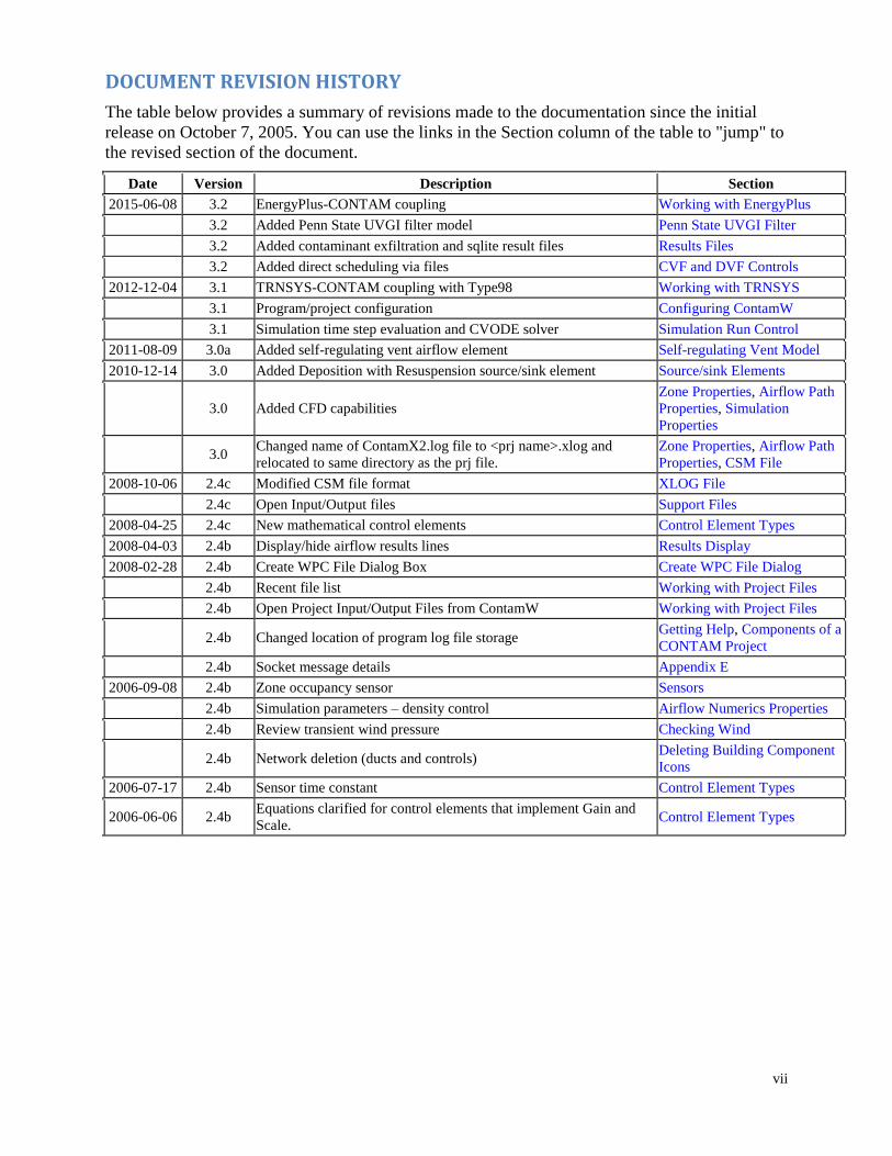
DOCUMENT REVISION HISTORY
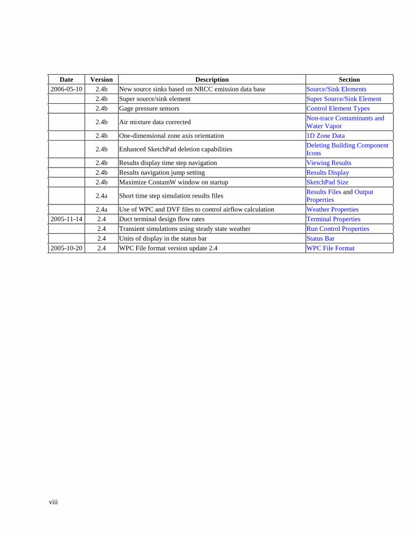
The table below provides a summary of revisions made to the documentation since the initial
release on October 7, 2005. You can use the links in the Section column of the table to "jump" to
the revised section of the document.
Date Version Description Section
2015-06-08 3.2 EnergyPlus-CONTAM coupling Working with EnergyPlus
3.2 Added Penn State UVGI filter model Penn State UVGI Filter
3.2 Added contaminant exfiltration and sqlite result files Results Files
3.2 Added direct scheduling via files CVF and DVF Controls
2012-12-04 3.1 TRNSYS-CONTAM coupling with Type98 Working with TRNSYS
3.1 Program/project configuration Configuring ContamW
3.1 Simulation time step evaluation and CVODE solver Simulation Run Control
2011-08-09 3.0a Added self-regulating vent airflow element Self-regulating Vent Model
2010-12-14 3.0 Added Deposition with Resuspension source/sink element Source/sink Elements
3.0 Added CFD capabilities
Zone Properties, Airflow Path
Properties, Simulation
Properties
3.0 Changed name of ContamX2.log file to <prj name>.xlog and
relocated to same directory as the prj file.
Zone Properties, Airflow Path
Properties, CSM File
2008-10-06 2.4c Modified CSM file format XLOG File
2.4c Open Input/Output files Support Files
2008-04-25 2.4c New mathematical control elements Control Element Types
2008-04-03 2.4b Display/hide airflow results lines Results Display
2008-02-28 2.4b Create WPC File Dialog Box Create WPC File Dialog
2.4b Recent file list Working with Project Files
2.4b Open Project Input/Output Files from ContamW Working with Project Files
2.4b Changed location of program log file storage Getting Help, Components of a
CONTAM Project
2.4b Socket message details Appendix E
2006-09-08 2.4b Zone occupancy sensor Sensors
2.4b Simulation parameters – density control Airflow Numerics Properties
2.4b Review transient wind pressure Checking Wind
2.4b Network deletion (ducts and controls) Deleting Building Component
Icons
2006-07-17 2.4b Sensor time constant Control Element Types
2006-06-06 2.4b Equations clarified for control elements that implement Gain and
Scale. Control Element Types
viii
Date Version Description Section
2006-05-10 2.4b New source sinks based on NRCC emission data base Source/Sink Elements
2.4b Super source/sink element Super Source/Sink Element
2.4b Gage pressure sensors Control Element Types
2.4b Air mixture data corrected Non-trace Contaminants and
Water Vapor
2.4b One-dimensional zone axis orientation 1D Zone Data
2.4b Enhanced SketchPad deletion capabilities Deleting Building Component
Icons
2.4b Results display time step navigation Viewing Results
2.4b Results navigation jump setting Results Display
2.4b Maximize ContamW window on startup SketchPad Size
2.4a Short time step simulation results files Results Files and Output
Properties
2.4a Use of WPC and DVF files to control airflow calculation Weather Properties
2005-11-14 2.4 Duct terminal design flow rates Terminal Properties
2.4 Transient simulations using steady state weather Run Control Properties
2.4 Units of display in the status bar Status Bar
2005-10-20 2.4 WPC File format version update 2.4 WPC File Format
ix
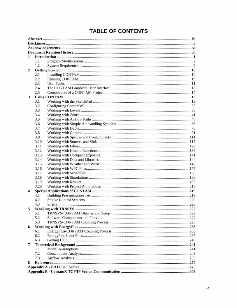
TABLE OF CONTENTS
Abstract ........................................................................................................................................................ iii Disclaimer ..................................................................................................................................................... iv Acknowledgements ...................................................................................................................................... vi Document Revision History ....................................................................................................................... vii 1 Introduction ............................................................................................................................................1
1.1 Program Modifications ................................................................................................................2 1.2 System Requirements ..................................................................................................................9
2 Getting Started ..................................................................................................................................... 10 2.1 Installing CONTAM .................................................................................................................. 10 2.2 Running CONTAM ................................................................................................................... 10 2.3 User Tasks ................................................................................................................................. 11 2.4 The CONTAM Graphical User Interface................................................................................... 13 2.5 Components of a CONTAM Project.......................................................................................... 15
3 Using CONTAM ................................................................................................................................... 19 3.1 Working with the SketchPad ..................................................................................................... 19 3.2 Configuring ContamW .............................................................................................................. 33 3.3 Working with Levels ................................................................................................................. 38 3.4 Working with Zones .................................................................................................................. 41 3.5 Working with Airflow Paths ...................................................................................................... 46 3.6 Working with Simple Air-handling Systems ............................................................................. 66 3.7 Working with Ducts ................................................................................................................... 73 3.8 Working with Controls .............................................................................................................. 91 3.9 Working with Species and Contaminants ................................................................................ 111 3.10 Working with Sources and Sinks ............................................................................................. 117 3.11 Working with Filters ................................................................................................................ 129 3.12 Working with Kinetic Reactions .............................................................................................. 137 3.13 Working with Occupant Exposure ........................................................................................... 141 3.14 Working with Data and Libraries ............................................................................................ 144 3.15 Working with Weather and Wind ............................................................................................ 149 3.16 Working with WPC Files ......................................................................................................... 157 3.17 Working with Schedules .......................................................................................................... 165 3.18 Working with Simulations ....................................................................................................... 169 3.19 Working with Results .............................................................................................................. 185 3.20 Working with Project Annotations .......................................................................................... 218
4 Special Applications of CONTAM .................................................................................................... 219 4.1 Building Pressurization Test .................................................................................................... 219 4.2 Smoke Control Systems ........................................................................................................... 220 4.3 Shafts ....................................................................................................................................... 220
5 Working with TRNSYS ..................................................................................................................... 222 5.1 TRNSYS-CONTAM Utilities and Setup ................................................................................. 222 5.2 Software Components and Files .............................................................................................. 222 5.3 TRNSYS-CONTAM Coupling Process .................................................................................. 223
6 Working with EnergyPlus ................................................................................................................. 233 6.1 EnergyPlus-CONTAM Coupling Process ............................................................................... 235 6.2 EnergyPlus Input Files ............................................................................................................. 238 6.3 Getting Help ............................................................................................................................ 240
7 Theoretical Background .................................................................................................................... 241 7.1 Model Assumptions ................................................................................................................. 241 7.2 Contaminant Analysis .............................................................................................................. 243 7.3 Airflow Analysis ...................................................................................................................... 253
8 References ........................................................................................................................................... 270 Appendix A - PRJ File Format ................................................................................................................. 275 Appendix B - ContamX TCP/IP Socket Communication ...................................................................... 309

x

Introduction – Program Modifications
1
1 INTRODUCTION
CONTAM is a multizone indoor air quality and ventilation analysis computer program designed
to help you determine:
Airflow Rates: infiltration, exfiltration, and room-to-room airflow rates in building
systems driven by mechanical means, wind pressures acting on the exterior of the building,
and buoyancy effects induced by the indoor and outdoor air temperature difference.
Contaminant Concentrations: the dispersal of airborne contaminants transported by these
airflows; transformed by a variety of processes including chemical and radio-chemical
transformation, adsorption and desorption to building materials, filtration, and deposition
and resuspension to and from building surfaces, etc.; and generated by a variety of source
mechanisms.
Personal Exposure: the prediction of exposure of occupants to airborne contaminants for
eventual risk assessment.
CONTAM can be useful in a variety of applications. Its ability to calculate building airflow rates
and relative pressures between zones of the building is useful for assessing the adequacy of
ventilation rates in a building, for determining the variation in ventilation rates over time, for
determining the distribution of ventilation air within a building, and for estimating the impact of
envelope air-tightening efforts on infiltration rates, and for evaluating the energy impacts of
building airflows. The program has also been used extensively for the design and analysis of
smoke management systems [Klote, et al. 2012]. The prediction of contaminant concentrations
can be used to determine the indoor air quality performance of buildings before they are
constructed and occupied, to investigate the impacts of various design decisions related to
ventilation systems and building material selection, to evaluate indoor air quality control
technologies, and to assess the indoor air quality performance of existing buildings. Predicted
contaminant concentrations can also be used to estimate personal exposure based on occupancy
patterns.
This document addresses both the graphical user interface (referred to herein as ContamW) and
the numerical solver (referred to herein as ContamX) of the program, collectively referred to as
CONTAM.

Introduction – Program Modifications
2
1.1 PROGRAM MODIFICATIONS
Program Enhancements CONTAM 3.2 is the latest version in the line of CONTAM programs. The history of major
enhancements is provided below. The latest version of CONTAM is backwards compatible with
previous versions, meaning you can open existing project files created with previous versions.
Once updated to the latest version of the program, project files can not be saved as or opened
with previous versions. Therefore, you should maintain older copies of your existing project
files.
Throughout this manual you will find new features (latest revision) of the program highlighted as
illustrated by this paragraph.
Version 3.2 EnergyPlus-CONTAM Multizone Airflow, Heat Transfer and Contaminant Analysis - This
capability includes modifications to ContamX and the creation of a new dynamic link library
(DLL) that implements co-simulation between EnergyPlus and ContamX via the Functional
Mockup Interface (FMI). This includes the development of ContamFMU.dll and enhancing
CONTAM3DExport.exe to enable the creation of EnergyPlus input files for the purposes of
performing co-simulation.
Contaminant Exfiltration Result Files - Added the ability to create result files that provide the
mass of contaminants that are transported to ambient.
SQLite Database Result Files - Added the ability to create a SQLite database file (.sqlite3) that
contains the same results as the simulation results file (.sim).
UVGI Filter - Added an ultra-violet germicidal irradiation filter element.
Direct Scheduling via CVF and DVF Controls - Added the ability to directly schedule items,
e.g., source/sinks and airflow paths, via external files without an associated controls networks
drawn on the SketchPad.
Version 3.1 TRNSYS-CONTAM Multizone Airflow, Heat Transfer and Contaminant Analysis - This
capability includes modifications to ContamW and ContamX and the creation of a new TRNSYS
Type and the software utilities to provide a new coupling process that enables ContamX to be
more directly coupled with TRNSYS Type56.
ContamW Pseudo-geometry - Provide ability to define scaling factor for drawing on the
ContamW SketchPad and view wall dimensions on the SketchPad. This feature is an aid to
utilities provided for the TRNSYS-CONTAM coupling that create three-dimensional
representations for TRNSYS Type56 multizone heat transfer calculation.
ContamW Temperature Plots - Provide ability to plot temperatures in ContamW.
ContamX - Added socket communication messages that provide for the transfer of
temperatures and airflow to/from ContamX.
Type98 - Acts as a bridge between ContamX and Type56 for TRNSYS simulations.
Introduction – Program Modifications
3
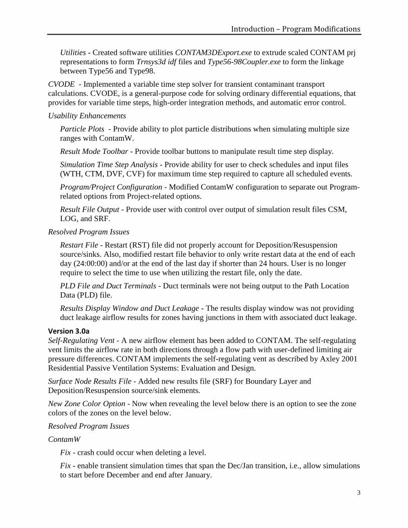
Utilities - Created software utilities CONTAM3DExport.exe to extrude scaled CONTAM prj
representations to form Trnsys3d idf files and Type56-98Coupler.exe to form the linkage
between Type56 and Type98.
CVODE - Implemented a variable time step solver for transient contaminant transport
calculations. CVODE, is a general-purpose code for solving ordinary differential equations, that
provides for variable time steps, high-order integration methods, and automatic error control.
Usability Enhancements
Particle Plots - Provide ability to plot particle distributions when simulating multiple size
ranges with ContamW.
Result Mode Toolbar - Provide toolbar buttons to manipulate result time step display.
Simulation Time Step Analysis - Provide ability for user to check schedules and input files
(WTH, CTM, DVF, CVF) for maximum time step required to capture all scheduled events.
Program/Project Configuration - Modified ContamW configuration to separate out Program-
related options from Project-related options.
Result File Output - Provide user with control over output of simulation result files CSM,
LOG, and SRF.
Resolved Program Issues
Restart File - Restart (RST) file did not properly account for Deposition/Resuspension
source/sinks. Also, modified restart file behavior to only write restart data at the end of each
day (24:00:00) and/or at the end of the last day if shorter than 24 hours. User is no longer
require to select the time to use when utilizing the restart file, only the date.
PLD File and Duct Terminals - Duct terminals were not being output to the Path Location
Data (PLD) file.
Results Display Window and Duct Leakage - The results display window was not providing
duct leakage airflow results for zones having junctions in them with associated duct leakage.
Version 3.0a Self-Regulating Vent - A new airflow element has been added to CONTAM. The self-regulating
vent limits the airflow rate in both directions through a flow path with user-defined limiting air
pressure differences. CONTAM implements the self-regulating vent as described by Axley 2001
Residential Passive Ventilation Systems: Evaluation and Design.
Surface Node Results File - Added new results file (SRF) for Boundary Layer and
Deposition/Resuspension source/sink elements.
New Zone Color Option - Now when revealing the level below there is an option to see the zone
colors of the zones on the level below.
Resolved Program Issues
ContamW
Fix - crash could occur when deleting a level.
Fix - enable transient simulation times that span the Dec/Jan transition, i.e., allow simulations
to start before December and end after January.

Introduction – Program Modifications
4
Fix - when replacing a wind pressure profile with the Find & Replace dialog the wall azimuth
and wind speed modifier should be set to the defaults.
Fix - allow plotting of results for a simulation that spans the Dec/Jan transition.
Fix - crash occurred when deleting zones having occupancy schedules that referenced them.
Fix - incorrect painting of the toolbar for some Windows themes.
Fix - cubic spline airflow element curves were not plotted correctly if their curves were
invalid.
Modification - consolidated variable density airflow calculation parameters.
ContamX
Fix - Matrix reordering issue when very large project files encountered fatal errors when
matrix reordering was attempted due to size of index parameter.
Fix - Prevent intermittent program crash when running under Windows 7 64 bit OS.
Fix - Contaminant summary file (CSM) issues: values when working with non-trace
boundary layer diffusion and deposition/resuspension source sinks were likely too high due
to summation of the source contributions over multiple iterations of the variable density
iterations within each time step; combinations of non-trace and trace contaminants could
result in trace contaminant-related summations not being accounted for. However, these issue
did not affect sim file results.
Fix - Issue related to non-trace contaminant calculations involving Boundary Layer Diffusion
and Deposition/Resuspension sources whereby the contribution of mass added to the zone in
which these source/sinks were located was incorrectly calculated.
Fix - Issues related to Deposition with Resuspension source/sink element when performing
variable density calculations.
Fix - Power Law source/sink model was not utilizing the correct source/sink element
function.
Fix - Enable DVF files to handle Dec/Jan transition.
Fix - Issues related to Decaying (exponential decay) source elements: generation rate was not
reset when scheduling the source on/off, and the generation rate was being compounded
when multiple Decaying sources were being used.
Modification - Improved variable density calculations.
Version 3.0 Coupled Multizone/CFD - Implemented the ability to simulate an internal zone using
computational fluid dynamics (CFD). Details of this capability are provided via the NIST
Multizone Modeling website.
Deposition/Resuspension Source/Sink Element - Added a new source/sink element that accounts
for both deposition and resuspension of particle contaminants to/from a surface.
Windows 7 64-bit - ContamX crashed intermittently due to data copy error.
Usability Enhancements
Introduction – Program Modifications
5
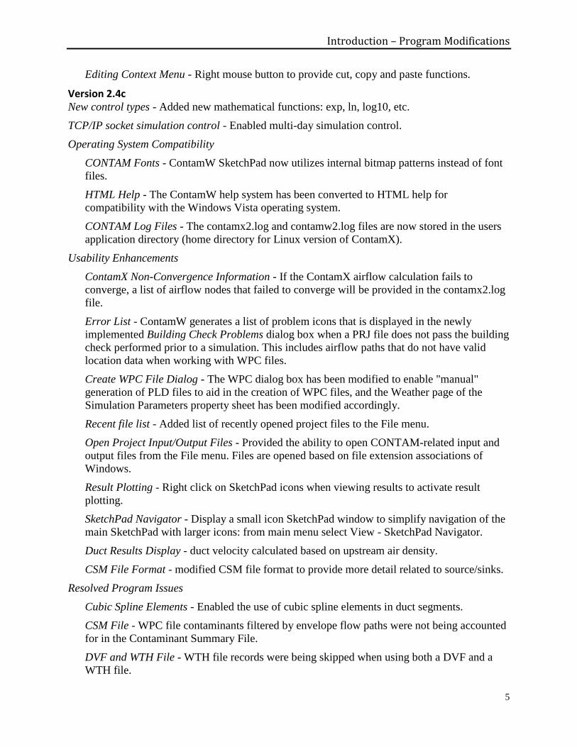
Editing Context Menu - Right mouse button to provide cut, copy and paste functions.
Version 2.4c New control types - Added new mathematical functions: exp, ln, log10, etc.
TCP/IP socket simulation control - Enabled multi-day simulation control.
Operating System Compatibility
CONTAM Fonts - ContamW SketchPad now utilizes internal bitmap patterns instead of font
files.
HTML Help - The ContamW help system has been converted to HTML help for
compatibility with the Windows Vista operating system.
CONTAM Log Files - The contamx2.log and contamw2.log files are now stored in the users
application directory (home directory for Linux version of ContamX).
Usability Enhancements
ContamX Non-Convergence Information - If the ContamX airflow calculation fails to
converge, a list of airflow nodes that failed to converge will be provided in the contamx2.log
file.
Error List - ContamW generates a list of problem icons that is displayed in the newly
implemented Building Check Problems dialog box when a PRJ file does not pass the building
check performed prior to a simulation. This includes airflow paths that do not have valid
location data when working with WPC files.
Create WPC File Dialog - The WPC dialog box has been modified to enable "manual"
generation of PLD files to aid in the creation of WPC files, and the Weather page of the
Simulation Parameters property sheet has been modified accordingly.
Recent file list - Added list of recently opened project files to the File menu.
Open Project Input/Output Files - Provided the ability to open CONTAM-related input and
output files from the File menu. Files are opened based on file extension associations of
Windows.
Result Plotting - Right click on SketchPad icons when viewing results to activate result
plotting.
SketchPad Navigator - Display a small icon SketchPad window to simplify navigation of the
main SketchPad with larger icons: from main menu select View - SketchPad Navigator.
Duct Results Display - duct velocity calculated based on upstream air density.
CSM File Format - modified CSM file format to provide more detail related to source/sinks.
Resolved Program Issues
Cubic Spline Elements - Enabled the use of cubic spline elements in duct segments.
CSM File - WPC file contaminants filtered by envelope flow paths were not being accounted
for in the Contaminant Summary File.
DVF and WTH File - WTH file records were being skipped when using both a DVF and a
WTH file.
Introduction – Program Modifications
6
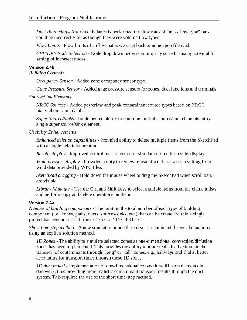
Duct Balancing - After duct balance is performed the flow rates of "mass flow type" fans
could be incorrectly set as though they were volume flow types.
Flow Limits - Flow limits of airflow paths were set back to none upon file read.
CVF/DVF Node Selection - Node drop down list was improperly sorted causing potential for
setting of incorrect nodes.
Version 2.4b Building Controls
Occupancy Sensor - Added zone occupancy sensor type.
Gage Pressure Sensor - Added gage pressure sensors for zones, duct junctions and terminals.
Source/Sink Elements
NRCC Sources - Added powerlaw and peak contaminant source types based on NRCC
material emission database.
Super Source/Sinks - Implemented ability to combine multiple source/sink elements into a
single super source/sink element.
Usability Enhancements
Enhanced deletion capabilities - Provided ability to delete multiple items from the SketchPad
with a single deletion operation.
Results display - Improved control over selection of simulation time for results display.
Wind pressure display - Provided ability to review transient wind pressures resulting from
wind data provided by WPC files.
SketchPad dragging - Hold down the mouse wheel to drag the SketchPad when scroll bars
are visible.
Library Manager - Use the Ctrl and Shift keys to select multiple items from the element lists
and perform copy and delete operations on them.
Version 2.4a Number of building components - The limit on the total number of each type of building
component (i.e., zones, paths, ducts, sources/sinks, etc.) that can be created within a single
project has been increased from 32 767 to 2 147 483 647.
Short time-step method - A new simulation mode that solves contaminant dispersal equations
using an explicit solution method.
1D Zones - The ability to simulate selected zones as one-dimensional convection/diffusion
zones has been implemented. This provides the ability to more realistically simulate the
transport of contaminants through "long" or "tall" zones, e.g., hallways and shafts, better
accounting for transport times through these 1D zones.
1D duct model - Implementation of one-dimensional convection/diffusion elements in
ductwork, thus providing more realistic contaminant transport results through the duct
system. This requires the use of the short time-step method.

Introduction – Program Modifications
7
Duct temperature calculations - When simulating 1D ducts in the short time-step mode,
CONTAM can now calculate duct temperatures based on the "mixing" of air streams at the
duct junctions and the source (zone) air temperatures from which air is introduced into the
duct system.
Simulation results data - Modified the zone and junction pressures as reported to the simulation
results file to more closely resemble gage pressures. Zone pressures are now referenced to the
ambient pressure at the level on which the zone is located. Junction static pressure is now
referenced to the zone in which the junction is located at the height of the junction within the
zone.
Automated duct balancing - Added simulation option to automatically balance duct systems.
This will greatly simplify the task of defining detailed duct systems in CONTAM.
Building model verification tests
Building pressurization test - Simulation option to automatically determine building envelope
airtightness based on a simulated fan pressurization test.
Building airflow test - Simulation option that generates a set of data, mostly related to
building ventilation, that can be used to gauge the reasonableness of model inputs before
beginning analysis of a building.
Cubic spline airflow elements
Contaminant Filters
New filter models - CONTAM has added particle and gaseous filter models that greatly
increases the user-s flexibility to create models based on measured filter performance data,
e.g., MERV and breakthrough curves.
Filter super elements - enables multiple filter models to be combined into a single filter
element, e.g., a particle pre-filter combined with a gaseous filter.
Contaminant summary file - This file is generated when simulating contaminants to provide
information related to source/sink contaminant generation and removal, filter loading and
breakthrough, and contaminant transport between building zones and ambient.
Deposition sink models - Added Deposition Velocity and Deposition Rate sink models to
simplify the definition of sinks based on more familiar deposition terminology.
Control super elements - The task of creating building control systems has been improved by
reducing the amount of user input required, increasing the amount of flexibility in defining
control systems and enabling the sharing of control elements, e.g., sensors, within and between
projects.
TCP/IP socket simulation control - ContamX can be controlled via the TCP/IP Socket
communication protocol based on a pre-defined set of messages that include control commands
and data exchange. ContamX can also be compiled and run under Linux based operating
systems, and a Linux-compatible executable is now available on the NIST web site.
Usability enhancements
Find - search for items on SketchPad by Name and Number
Find-and-replace - search for and replace properties of building components within a project
Introduction – Program Modifications
8
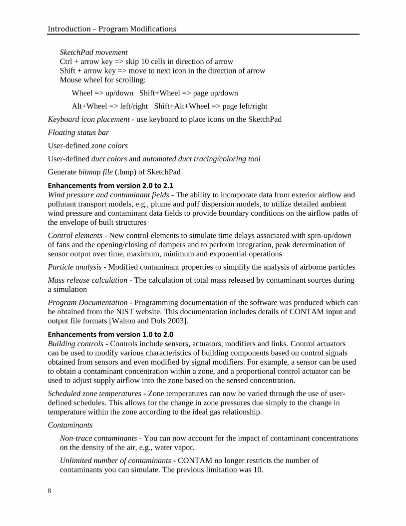
SketchPad movement
Ctrl + arrow key => skip 10 cells in direction of arrow
Shift + arrow key => move to next icon in the direction of arrow
Mouse wheel for scrolling:
Wheel => up/down Shift+Wheel => page up/down
Alt+Wheel => left/right Shift+Alt+Wheel => page left/right
Keyboard icon placement - use keyboard to place icons on the SketchPad
Floating status bar
User-defined zone colors
User-defined duct colors and automated duct tracing/coloring tool
Generate bitmap file (.bmp) of SketchPad
Enhancements from version 2.0 to 2.1 Wind pressure and contaminant fields - The ability to incorporate data from exterior airflow and
pollutant transport models, e.g., plume and puff dispersion models, to utilize detailed ambient
wind pressure and contaminant data fields to provide boundary conditions on the airflow paths of
the envelope of built structures
Control elements - New control elements to simulate time delays associated with spin-up/down
of fans and the opening/closing of dampers and to perform integration, peak determination of
sensor output over time, maximum, minimum and exponential operations
Particle analysis - Modified contaminant properties to simplify the analysis of airborne particles
Mass release calculation - The calculation of total mass released by contaminant sources during
a simulation
Program Documentation - Programming documentation of the software was produced which can
be obtained from the NIST website. This documentation includes details of CONTAM input and
output file formats [Walton and Dols 2003].
Enhancements from version 1.0 to 2.0 Building controls - Controls include sensors, actuators, modifiers and links. Control actuators
can be used to modify various characteristics of building components based on control signals
obtained from sensors and even modified by signal modifiers. For example, a sensor can be used
to obtain a contaminant concentration within a zone, and a proportional control actuator can be
used to adjust supply airflow into the zone based on the sensed concentration.
Scheduled zone temperatures - Zone temperatures can now be varied through the use of user-
defined schedules. This allows for the change in zone pressures due simply to the change in
temperature within the zone according to the ideal gas relationship.
Contaminants
Non-trace contaminants - You can now account for the impact of contaminant concentrations
on the density of the air, e.g., water vapor.
Unlimited number of contaminants - CONTAM no longer restricts the number of
contaminants you can simulate. The previous limitation was 10.
Introduction – System Requirements
9
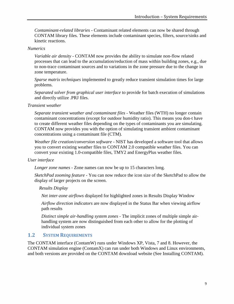
Contaminant-related libraries - Contaminant related elements can now be shared through
CONTAM library files. These elements include contaminant species, filters, source/sinks and
kinetic reactions.
Numerics
Variable air density - CONTAM now provides the ability to simulate non-flow related
processes that can lead to the accumulation/reduction of mass within building zones, e.g., due
to non-trace contaminant sources and to variations in the zone pressure due to the change in
zone temperature.
Sparse matrix techniques implemented to greatly reduce transient simulation times for large
problems.
Separated solver from graphical user interface to provide for batch execution of simulations
and directly utilize .PRJ files.
Transient weather
Separate transient weather and contaminant files - Weather files (WTH) no longer contain
contaminant concentrations (except for outdoor humidity ratio). This means you don-t have
to create different weather files depending on the types of contaminants you are simulating.
CONTAM now provides you with the option of simulating transient ambient contaminant
concentrations using a contaminant file (CTM).
Weather file creation/conversion software - NIST has developed a software tool that allows
you to convert existing weather files to CONTAM 2.0 compatible weather files. You can
convert your existing 1.0-compatible files, TMY2 and EnergyPlus weather files.
User interface
Longer zone names - Zone names can now be up to 15 characters long.
SketchPad zooming feature - You can now reduce the icon size of the SketchPad to allow the
display of larger projects on the screen.
Results Display
Net inter-zone airflows displayed for highlighted zones in Results Display Window
Airflow direction indicators are now displayed in the Status Bar when viewing airflow
path results
Distinct simple air-handling system zones - The implicit zones of multiple simple air-
handling system are now distinguished from each other to allow for the plotting of
individual system zones
1.2 SYSTEM REQUIREMENTS
The CONTAM interface (ContamW) runs under Windows XP, Vista, 7 and 8. However, the
CONTAM simulation engine (ContamX) can run under both Windows and Linux environments,
and both versions are provided on the CONTAM download website (See Installing CONTAM).
Getting Started – Installing CONTAM
10
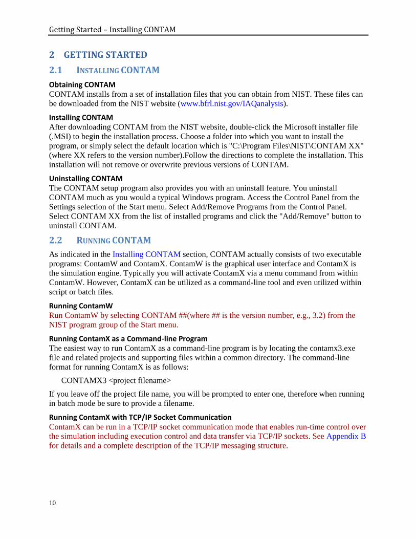
2 GETTING STARTED
2.1 INSTALLING CONTAM
Obtaining CONTAM CONTAM installs from a set of installation files that you can obtain from NIST. These files can
be downloaded from the NIST website (www.bfrl.nist.gov/IAQanalysis).
Installing CONTAM After downloading CONTAM from the NIST website, double-click the Microsoft installer file
(.MSI) to begin the installation process. Choose a folder into which you want to install the
program, or simply select the default location which is "C:\Program Files\NIST\CONTAM XX"
(where XX refers to the version number).Follow the directions to complete the installation. This
installation will not remove or overwrite previous versions of CONTAM.
Uninstalling CONTAM The CONTAM setup program also provides you with an uninstall feature. You uninstall
CONTAM much as you would a typical Windows program. Access the Control Panel from the
Settings selection of the Start menu. Select Add/Remove Programs from the Control Panel.
Select CONTAM XX from the list of installed programs and click the "Add/Remove" button to
uninstall CONTAM.
2.2 RUNNING CONTAM
As indicated in the Installing CONTAM section, CONTAM actually consists of two executable
programs: ContamW and ContamX. ContamW is the graphical user interface and ContamX is
the simulation engine. Typically you will activate ContamX via a menu command from within
ContamW. However, ContamX can be utilized as a command-line tool and even utilized within
script or batch files.
Running ContamW Run ContamW by selecting CONTAM ##(where ## is the version number, e.g., 3.2) from the
NIST program group of the Start menu.
Running ContamX as a Command-line Program The easiest way to run ContamX as a command-line program is by locating the contamx3.exe
file and related projects and supporting files within a common directory. The command-line
format for running ContamX is as follows:
CONTAMX3 <project filename>
If you leave off the project file name, you will be prompted to enter one, therefore when running
in batch mode be sure to provide a filename.
Running ContamX with TCP/IP Socket Communication ContamX can be run in a TCP/IP socket communication mode that enables run-time control over
the simulation including execution control and data transfer via TCP/IP sockets. See Appendix B
for details and a complete description of the TCP/IP messaging structure.
Getting Started – User Tasks
11
2.3 USER TASKS
The use of CONTAM to analyze airflow or contaminant migration in a building involves five
distinct tasks:
1. Building Idealization: Form an idealization or specific model of the building being
considered,
2. Schematic Representation: Develop a schematic representation of the idealized building
using the ContamW SketchPad to draw the building components,
3. Define Building Components: Collect and input data associated with each of the building
components represented on the SketchPad,
4. Simulation: Select the type of analysis you wish to conduct, set simulation parameters, and
execute the simulation,
5. Review & Record Results: Review the results of your simulation and record selected
portions of the results.
Task 1 - Building Idealization Building idealization refers to the simplification of a building into a set of zones that are relevant
to the user's goal in performing an analysis. A building can be idealized in a number of ways
depending on the building layout, the ventilation system configuration and the problem of
interest. This idealization phase of analysis requires some engineering knowledge on the part of
the user and is an acquired skill that you can develop through experience in airflow and indoor
air quality analysis and by becoming familiar with the theoretical principles and details upon
which indoor air quality analysis is based.
It is important to note that CONTAM provides a macroscopic model of a building. In this
macroscopic view, each zone is considered to be well-mixed. Well-mixed means that a zone is
characterized by a discrete set of state variables, i.e., temperature, pressure and contaminant
concentrations. Temperature and contaminant concentration do not vary spatially within a zone,
and contaminants mix instantly throughout well-mixed zones. However, pressure does vary
hydrostatically within all zones.
Beginning with CONTAM version 2.4, one-dimensional convection/diffusion zones can be
implemented within CONTAM. This feature can be useful in simulating contaminant transport
through long or tall zones that are characterized by a single, dominant flow direction. One
dimensional convection/diffusion duct models can also be implemented to more realistically
capture contaminant transport within entire duct systems.
CONTAM is well suited for analyzing the interaction between the zones of a building on a
macroscopic or whole-building level. Computational Fluid Dynamics (CFD) analysis is well-
suited for analyzing the airflow and contaminant transport characteristics on a microscopic level,
i.e., within a single zone of a building. However, the computational resources required to
perform a CFD analysis for an entire building is currently prohibitive. Beginning with CONTAM
version 3.0, a zero-order turbulence CFD model has been directly integrated with CONTAM to
enable consideration of a single, CFD zone in conjunction with the rest of a building that is being
analyzed on a macroscopic level, i.e., coupled multizone/CFD analysis.
Getting Started – User Tasks
12
Task 2 - SketchPad Representation Developing the SketchPad representation will be the focus of your interaction with ContamW.
With ContamW's SketchPad you will be able to draw a diagram – a SketchPad diagram – of
your building idealization using drawing tools and sets of icons to represent components of the
building system. CONTAM translates your diagram into a system of equations that will than be
used to model the behavior of the building when you perform a simulation.
See Working with the SketchPad in the Using CONTAMW section.
Task 3 Data Entry Data entry can be one of the more time-consuming parts of the process of using ContamW. It
involves the determination and input of the numerical values of the parameters associated with
each of the SketchPad icons. These icons represent the elements of the building model and
include air leakage paths (windows, doors, cracks), ventilation system elements (fans, ducts,
vents), contaminant sources, filters, and sinks and control network components. Each of these
elements is associated with a number of parameters, and you must obtain the values of these
parameters for entry into the model. Depending on the element and the application, these values
can be obtained from building-specific data, engineering handbooks, and product literature. In
many cases, a degree of engineering judgement will be involved. ContamW allows you to create
libraries of these elements that you can use in current and future modeling efforts.
Detailed information is provided for the various components throughout the Using CONTAMW
section.
Task 4 Simulation Simulation is the use of CONTAM to solve the system of equations assembled from your
SketchPad representation of a building to predict the airflow and contaminant concentrations of
interest. This step involves determining the type of analysis that is needed; steady state, transient
or cyclical, and a number of other simulation parameters. These parameters depend on the type
of analysis you wish to perform (steady state or transient), and include convergence criteria and
in the case of a transient analysis, time steps and the duration of the analysis.
See Working with Simulations in the Using CONTAMW section.
Task 5 Review & Record Results ContamW allows you to view the simulation results on the screen and to output them to a file for
input to a spreadsheet program or other data analysis programs including those developed by
NIST and available on the CONTAM website (e.g., SimRead2 and ContamRV). Airflows and
pressure differences at each flow element can be viewed directly on the SketchPad. Contaminant
concentrations for a zone can also be plotted as a function of time directly from the SketchPad.
You can then decide which data you wish to examine more closely and export these to a tab-
delimited text file that can then be imported into a spreadsheet for further analysis. There is also
a controls-related feature that provide the ability to report the values of user-selected control
nodes to a control "log" file for each time step of a transient simulation.
See Working with Results in the Using CONTAMW section.
Getting Started – The CONTAM Graphical User Interface
13
2.4 THE CONTAM GRAPHICAL USER INTERFACE
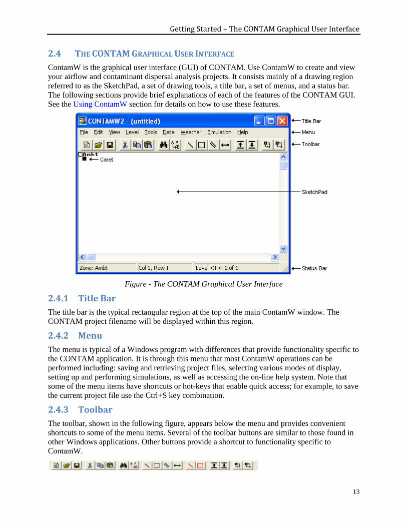
ContamW is the graphical user interface (GUI) of CONTAM. Use ContamW to create and view
your airflow and contaminant dispersal analysis projects. It consists mainly of a drawing region
referred to as the SketchPad, a set of drawing tools, a title bar, a set of menus, and a status bar.
The following sections provide brief explanations of each of the features of the CONTAM GUI.
See the Using ContamW section for details on how to use these features.
Figure - The CONTAM Graphical User Interface
2.4.1 Title Bar
The title bar is the typical rectangular region at the top of the main ContamW window. The
CONTAM project filename will be displayed within this region.
2.4.2 Menu
The menu is typical of a Windows program with differences that provide functionality specific to
the CONTAM application. It is through this menu that most ContamW operations can be
performed including: saving and retrieving project files, selecting various modes of display,
setting up and performing simulations, as well as accessing the on-line help system. Note that
some of the menu items have shortcuts or hot-keys that enable quick access; for example, to save
the current project file use the Ctrl+S key combination.
2.4.3 Toolbar
The toolbar, shown in the following figure, appears below the menu and provides convenient
shortcuts to some of the menu items. Several of the toolbar buttons are similar to those found in
other Windows applications. Other buttons provide a shortcut to functionality specific to
ContamW.
Getting Started – The CONTAM Graphical User Interface
14
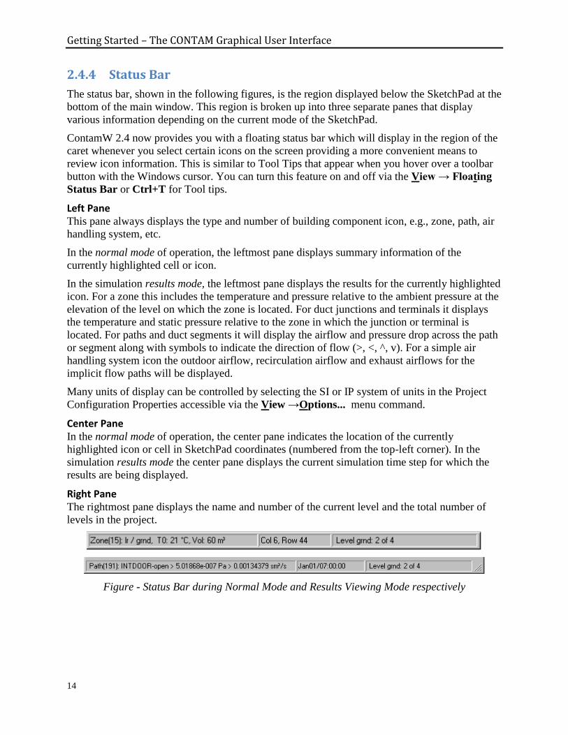
2.4.4 Status Bar
The status bar, shown in the following figures, is the region displayed below the SketchPad at the
bottom of the main window. This region is broken up into three separate panes that display
various information depending on the current mode of the SketchPad.
ContamW 2.4 now provides you with a floating status bar which will display in the region of the
caret whenever you select certain icons on the screen providing a more convenient means to
review icon information. This is similar to Tool Tips that appear when you hover over a toolbar
button with the Windows cursor. You can turn this feature on and off via the View → Floating
Status Bar or Ctrl+T for Tool tips.
Left Pane This pane always displays the type and number of building component icon, e.g., zone, path, air
handling system, etc.
In the normal mode of operation, the leftmost pane displays summary information of the
currently highlighted cell or icon.
In the simulation results mode, the leftmost pane displays the results for the currently highlighted
icon. For a zone this includes the temperature and pressure relative to the ambient pressure at the
elevation of the level on which the zone is located. For duct junctions and terminals it displays
the temperature and static pressure relative to the zone in which the junction or terminal is
located. For paths and duct segments it will display the airflow and pressure drop across the path
or segment along with symbols to indicate the direction of flow (>, <, ^, v). For a simple air
handling system icon the outdoor airflow, recirculation airflow and exhaust airflows for the
implicit flow paths will be displayed.
Many units of display can be controlled by selecting the SI or IP system of units in the Project
Configuration Properties accessible via the View →Options... menu command.
Center Pane In the normal mode of operation, the center pane indicates the location of the currently
highlighted icon or cell in SketchPad coordinates (numbered from the top-left corner). In the
simulation results mode the center pane displays the current simulation time step for which the
results are being displayed.
Right Pane The rightmost pane displays the name and number of the current level and the total number of
levels in the project.
Figure - Status Bar during Normal Mode and Results Viewing Mode respectively
Getting Started – Components of a CONTAM Project
15
2.5 COMPONENTS OF A CONTAM PROJECT
2.5.1 Project Files
All data related to the characteristics of the projects you work with are stored in a "project" file
having a "PRJ" extension (See Working with Project Files). This is an ASCII file, which is
intended to be "viewed" only by the ContamW program. You should keep careful records of
your project files and establish a naming convention that is meaningful to you for the various
versions of a project that you may wish to save. There are other files utilized by CONTAM
including: simulation results files, ambient files, library files, log files and other support files.
Results Files Simulation results are stored in files created automatically by ContamX with the same name as
the PRJ file except that the "PRJ" extension is replaced by extensions that depend on the type of
results generated by the simulation (see Working with Simulation Results).
Ambient Files Ambient files include weather (WTH extension), contaminant (CTM extension) and wind
pressure and contaminant files (WPC extension). Ambient files may contain up to a years worth
of data and are used when performing transient simulations (see Working with Weather). These
are ASCII files, but the formats are unique to CONTAM.
Library Files Library files are the means by which you can share various types of data between CONTAM
projects (see Working with Data and Libraries).
Support Files Support files include log files, backup files and a configuration file. ContamW support files are
created in the user's application directory - c:\Documents and Settings\<user>\Application
Data\NIST\ContamW\. The ContamX log file is created in c:\Documents and
Settings\<user>\Application Data\NIST\ContamX\. The Linux version of ContamX stores the
ContamX log file in the user's home directory. Log files contain information about the execution
of the respectful programs and are useful in the event that you require technical support from the
program developers (see Getting Help). ContamW creates a backup (BKP extension) file every
time a PRJ file is successfully opened. The configuration file (CFG extension) and the BKP file
are also stored in the ContamW application directory.
2.5.2 Building Components
Building components are the items that characterize the physical makeup of a building that you
define using ContamW. This section briefly describes these components.
Levels CONTAM represents buildings in terms of multiple levels, accounting for the communication of
air and contaminants between these levels. Levels typically correspond to floors of a building,
but a suspended ceiling acting as a return air plenum or a raised floor acting as a supply plenum
may also be treated as a level.
Getting Started – Components of a CONTAM Project
16
Walls Walls are used to designate zones which are regions surrounded by walls, floor and ceiling.
These walls include the building envelope and internal partitions with a significant resistance to
airflow.
Floors and Ceilings Floors and ceilings are included implicitly by ContamW for building zones. When you draw a
zone on the SketchPad, ContamW automatically includes the floor of the zone. To create a roof
with penetrations into the floor below requires a blank level above the top floor. It is also
possible to create a phantom zone with no floor or ceiling as might be required to create an
atrium that spans multiple levels (see Working with Zones).
Zones In CONTAM, a zone typically refers to a volume of air having a uniform temperature and
contaminant concentration. However, beginning with version 2.4, zones can now be configured
as one-dimensional convection/diffusion zones in which contaminant concentrations are allowed
to vary along a user-specified axis. Beginning with version 3.0 a single zone or region of a
building can be defined as a CFD zone.
There are three types of zones in CONTAM: normal, phantom and ambient. Normal zones are
separated from the zone below by a floor. The ambient zone, which surrounds the building is
implicitly defined and is identified by the symbol at the upper-left corner of the SketchPad. You
can also use an ambient zone icon to define a courtyard. Phantom zones indicate that the area on
the current level is actually part of the normal zone on the level immediately below. There is no
floor between a phantom zone and the normal zone below. You could use phantom zones to
define building features such as atriums. Only normal zones can be configured to be
convection/diffusion zones, however, these zones can still be referenced by phantom zones.
Airflow Paths An airflow path indicates some building feature by which air can move from one zone to
another. Such features include cracks in the building envelope, open doorways, and fans. Path
symbols placed on the walls are used to represent openings between zones or to ambient; any
other placement represents an opening in the floor to the zone on the level below. CONTAM can
implement several different models or airflow elements to define airflow paths. The basic
categories of airflow elements or models are as follows: small and large crack/openings
represented by power-law and quadratic pressure relationships, small and large doorways
elements, and fan/forced airflow elements. (See Working with Airflow Paths)
Simple Air-handling Systems The simple air-handling system (AHS) provides a simple means of introducing an air-handling
system into a building without having to draw a duct system. It provides a reasonable model of
an air-handling system that delivers user-specified flows where the system is properly balanced
and the fan is not impacted by any other pressurizing effects in the building. The AHS consists of
two implicit airflow nodes (return and supply), three implicit flow paths (recirculation, outdoor,
and exhaust air), and multiple supply and return points that you place within the zones of the
building. You can set the air flows of the AHS to vary according to a schedule.
Getting Started – Components of a CONTAM Project
17
Ducts You can use ducts to implement a more detailed model of an air-handling system that handles a
broader range of conditions. For example, when an air handler is off, the ductwork may provide
flow paths between zones which are significant in relation to the normal construction cracks or
openings. Ductwork consists of duct segments (paths) and junctions or terminal points (nodes).
CONTAM can implement several different duct segment models or duct flow elements to define
duct segments. The basic categories of duct flow elements are as follows: resistance models, fan
performance curves, and back-draft dampers. (See Working with Ducts)
Contaminants, Sources and Sinks You can define an unlimited number of contaminants within a single project with a practically
limitless number of sources associated with the contaminants. CONTAM can simulate
contaminant transport via airflow between zones, removal by filtration mechanisms associated
with flow paths, and removal and addition by chemical reaction. CONTAM can also implement
several source and sink models to generate contaminants within or remove contaminants from a
zone. These models include: constant generation, pressure driven, decaying source, cutoff
concentration, reversible boundary layer diffusion, and burst models. (See Working with
Contaminants and Working with Sources and Sinks)
Schedules Schedules are used to control or modify various properties of building components as a function
of time. You can set schedules for airflow paths, duct flow paths; contaminant sources and sinks;
and inlets, outlets and outdoor air delivery of simple air-handling systems. The effect of setting a
schedule on a building component varies depending on the properties of the component. For
example, you can set a schedule to adjust the airflow delivered to a zone by an inlet of a simple
air-handling system. (See Working with Simple Air Handling Systems) CONTAM also provides
the ability to schedule zone temperatures.
Controls Controls include sensors, actuators, modifiers and links. Control actuators can be used to modify
various characteristics of building components based on control signals obtained from sensors
and even modified by signal modifiers. For example, a sensor can be used to obtain a
contaminant concentration within a zone, and a proportional control actuator can be used to
adjust supply airflow into the zone based on the sensed concentration.
Occupants Occupants can be used to determine the amount of contaminant exposure a person would be
subjected to within a building. Occupants can also generate contaminants. You can set a schedule
to establish each occupant's movement within a building. Occupant schedules can also be used to
define periods of times when occupants are not in the building. (See Working with Occupant
Exposure)
2.5.3 Weather
CONTAM enables you to account for either steady-state or varying weather conditions. Weather
conditions consist of ambient temperature, barometric pressure, humidity ratio, wind speed and
direction, as well as ambient contaminant concentrations.

Getting Started – Components of a CONTAM Project
18
2.5.4 Simulation
In CONTAM, simulation is the process of forming a set of simultaneous equations based upon
the information stored in the project file, performing the numerical analysis to solve the set of
nodal equations according to user-defined specifications, and creating simulation results files that
can be viewed using the ContamW interface. There are three basic types of simulations that you
can perform for airflow and contaminant analysis using CONTAM: steady state, transient and
cyclical. (see Working with Simulations)
Using CONTAM – Working with the SketchPad
19
3 USING CONTAM
This section provides detailed information on how to use the features of the CONTAM program
as well as a detailed explanations of the terminology of the user interface.
3.1 WORKING WITH THE SKETCHPAD
The SketchPad is the region of the ContamW screen where you draw the schematic
representation of a building you wish to analyze. This representation is in the form of a set of
simplified floor plans that represent the levels of a building. The SketchPad consists of an
invisible array of cells into which you place various icons to form your schematics of a building.
The SketchPad is used to establish the geometric relationships of the relevant building features
and is not necessarily intended to produce a scaled representation of a building. It should be used
to create a simplified model where the walls, zones, and airflow paths are topologically similar to
the actual building.
Pseudo-Geometry While ContamW does not require you to draw building floor plans to scale, the SketchPad does
provide the ability to assign a scale value to the SketchPad cells. You can choose to display this
so-called pseudo-geometry via the Project Options of the ContamW Configuration. This will
provide dimensions in the status bar as you draw on the SketchPad. It will also provide you with
scaled information for walls, zones and ducts. It will provide wall areas when you highlight wall
icons, which can be useful when defining multipliers of airflow path icons associated with the
wall. When the pseudo-geometry mode is activated, default values will be provided for zone
volume (based on scaled floor area) and duct lengths. In order to distinguish between pseudo-
geometry values and actual values as saved in the prj file, scaled values will be enclosed in "{}"
when presented in the SketchPad Status Bar. This feature is intended to simplify the coupling
with energy analysis software, e.g., TRNSYS and EnergyPlus, which require geometric
information in order to perform energy related calculations (See Working with TRNSYS).
The Caret When working with ContamW you will notice a blinking square on the SketchPad. This is
known as the system caret, and it is the size of a single SketchPad cell. This caret is the same
thing as the blinking vertical bar that is common to many word processing applications. The
caret indicates the currently selected cell of the SketchPad. Any icon-related information that
appears in the status bar is associated with the location of the caret.
Moving the Caret To move the caret around the SketchPad you can use the keyboard arrow keys or you can move
the system cursor with the mouse and click the left mouse button to set the caret position. You
can also use the arrow keys in conjunction with the Shift and Ctrl keys to move the caret more
quickly.
Shift + Arrow Key moves the caret 10 cells in the direction of the arrow. The number of cells to
move can be modified within the ContamW Configuration (See Cell/Icon Size in the
Configuring ContamW section).
Ctrl + Arrow Key moves the caret to the next icon in the direction of the arrow
SketchPad Operations The specific operations that you will perform using the SketchPad are as follows:
Using CONTAM – Working with the SketchPad
20
1. Drawing Walls, Ducts and Controls
2. Drawing building component icons
3. Defining building component icons
4. Viewing results
5. Viewing envelope pressure differentials due to wind effects
SketchPad Modes There are three basic modes of the SketchPad: normal, results and wind pressure. The
SketchPad mode basically refers to the type of information that is displayed upon the SketchPad.
You can tell what mode the program is in by looking at the items in the View menu to see which
one has a mark next to it.
In the normal mode ContamW displays only the building component icons. In this mode
you can add, delete, copy, and move icons.
In the results mode, ContamW displays simulation results upon the SketchPad. In this
mode you will not be allowed to add, delete, copy and move icons upon the SketchPad (See Viewing Results).
The wind pressure mode is provided to verify wind speed and direction information
visually on the SketchPad (See Checking Wind Pressure Data).
Control Super Element / Super Node SketchPad With the advent of the new control super element, comes another use of the SketchPad to create
and edit super elements and super nodes (See Control Super Elements in the Working with
Controls section). When working with super elements only the controls drawing tool is enabled,
along with the ability to define the control network icons. This SketchPad is activated via the
Data→Controls→Super Elements… menu item. When the Super Element SketchPad is active,
the upper left corner of the SketchPad will display "Super Element:" followed by the name of the
super element currently displayed on the SketchPad. When working with super elements the
"Control Super Elements" dialog box will also be displayed. The Super Node SketchPad enables
only the modification of existing control sub-node icons, so the control drawing tool will be
disabled as will be the ability to delete control network icons. The Super Node SketchPad is
activated by instantiating an existing control super element or double-clicking on a Super Node
icon. When the Super Node SketchPad is active, the upper left corner of the SketchPad will
display "Super Node:" followed by the name of the super node currently displayed on the
SketchPad. When working with super nodes the "Super Node Data" dialog box will also be
displayed (See Control Super Nodes).
Zooming the SketchPad You can change the size of the cells in which icons appear on the SketchPad in order to zoom the
floor plan in and out on the SketchPad. The amount of information that will appear on your
screen is dependent on the resolution and the cell size. Zooming can be accomplished using the
two zoom buttons on the toolbar and their associated keyboard shortcuts shown below or
changing the Current Cell/Icon Size on the Cell/Icon Size page of the Project Configuration
Properties dialog box accessible via the View→Options... menu selection (see Cell/Icon Size).
Using CONTAM – Working with the SketchPad
21
Keyboard Shortcuts:
Ctrl + PageUp to increase cell size
Ctrl + PageDown to decrease cell size
Printing SketchPad Images You can obtain images of your SketchPad drawings to print or edit using the Windows print
screen feature. To do this, size the ContamW window and press Alt+PrintScrn on the keyboard
to copy the current window to the Windows clipboard. Then you can immediately paste the
image into the desired program. For example, you can paste the image into the Windows Paint
program for editing or directly into a word processing program. You can then print the image
from either of these programs.
Exporting .BMP SketchPad Files You can save a SketchPad image of the currently displayed level to a Windows bitmap (.BMP)
file using the File→Save SketchPad to .BMP File... menu item. The Save As dialog box will
appear allowing you to name the file. The file will contain the entire SketchPad based on the
current cell/icon size and color settings.
3.1.1 Drawing Walls, Ducts and Controls
You use various tools to draw the physical features of the building such as walls and ducts. All
drawing can be accomplished with either the mouse or the keyboard. When drawing, the
following mouse and keyboard keys produce common behavior. The left mouse button (LMB)
corresponds to the , or Enter key; the right mouse button (RMB) to the Esc key. Vertical
motion of the cursor corresponds to the and cursor keys, and horizontal motion corresponds
to the and → cursor keys.
The basic steps for drawing walls and ducts are as follows:
1. Activate drawing tool,
2. Set the initial location of the object,
3. Draw the object,
4. Undo current drawing,
5. Finalize drawing the object, and
6. Deactivate drawing tool.
Activating a Drawing Tool There are four drawing tools available, two for drawing walls, one for drawing ducts and one for
drawing control networks. To activate a drawing tool either select it from the toolbar, select it
from the "Tools" menu, or use the shortcut associated with the menu item. The toolbar button of
a selected drawing tool will remain depressed as long as that tool is active. The toolbar buttons
and associated menu shortcuts are shown here.
rectangle (or box) drawing tool (Ctrl+B)
free-form wall drawing tool (Ctrl+W)
duct drawing tool (Ctrl+D)
Using CONTAM – Working with the SketchPad
22
controls drawing tool (Ctrl+L)
Once you have selected the tool, the drawing cursor will be displayed. The drawing cursor is a
pink square the size of a single SketchPad cell. Initially, the cursor appears with a transparent
center.
Setting the Initial Location of the Object To begin drawing the object, you set the initial location by first moving the drawing cursor either
with the mouse or the keyboard arrow keys and then you either click the LMB or press on the
keyboard. This will anchor the beginning of the object at the nearest valid SketchPad cell for the
type of object you are drawing. When you select a valid beginning location, the drawing cursor
will become solid and you can begin drawing your object.
Drawing the Object After you anchor the beginning of the object, you simply use the mouse and/or keyboard arrow
keys to draw the desired shape. While you are drawing, the cursor will be restricted to the
SketchPad region and constrained to specific movements in order to maintain drawing within
valid cells of the SketchPad. As you move the cursor, a dark line will appear on the SketchPad
representing the shape of the object you are drawing.
You can also move more quickly using the Shift + Arrow Key and Ctrl + Arrow Key keyboard
combinations.
Shift + Arrow Key moves the drawing cursor 10 cells in the direction of the arrow. The number
of cells to move can be modified within the ContamW Configuration (See Cell/Icon Size in the
Configuring ContamW section).
Ctrl + Arrow Key moves the drawing cursor to the next icon in the direction of the arrow,
which may be a wall, duct or control.
Undoing the Current Drawing Prior to finalizing the drawing of the object, you can undo your drawing. To undo what you have
drawn, either single-click the RMB or press the Esc key. This will erase the thick dark line, but
you will still be in the drawing mode. To begin drawing again, set the initial location again and
continue drawing another object.
Finalizing the Drawing Object Once you are satisfied with your drawing, you finalize the object by either single-clicking the
LMB or pressing the key. This will replace the cells that had the thick dark line with the icons
appropriate for completing the type of object you are drawing. If you have attempted to draw an
invalid object, you will be prompted with a dialog box containing a message indicating the type
of error, and then you will be allowed to repair the drawn object.
Deactivating Drawing Tools When you are finished using a drawing tool you click the RMB or press Esc until your system
cursor reappears. Also, selecting a different drawing tool will automatically deactivate the
current tool if you do not currently have an object anchored.
3.1.2 Drawing Building Component Icons
A set of icons is used to represent various building components such as airflow paths
(representing doors, windows, cracks, etc.), contaminant sources and sinks, occupants and air-
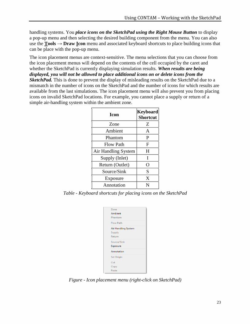
Using CONTAM – Working with the SketchPad
23
handling systems. You place icons on the SketchPad using the Right Mouse Button to display
a pop-up menu and then selecting the desired building component from the menu. You can also
use the Tools → Draw Icon menu and associated keyboard shortcuts to place building icons that
can be place with the pop-up menu.
The icon placement menus are context-sensitive. The menu selections that you can choose from
the icon placement menus will depend on the contents of the cell occupied by the caret and
whether the SketchPad is currently displaying simulation results. When results are being
displayed, you will not be allowed to place additional icons on or delete icons from the
SketchPad. This is done to prevent the display of misleading results on the SketchPad due to a
mismatch in the number of icons on the SketchPad and the number of icons for which results are
available from the last simulations. The icon placement menu will also prevent you from placing
icons on invalid SketchPad locations. For example, you cannot place a supply or return of a
simple air-handling system within the ambient zone.
Icon Keyboard
Shortcut
Zone Z
Ambient A
Phantom P
Flow Path F
Air Handling System H
Supply (Inlet) I
Return (Outlet) O
Source/Sink S
Exposure X
Annotation N
Table - Keyboard shortcuts for placing icons on the SketchPad
Figure - Icon placement menu (right-click on SketchPad)
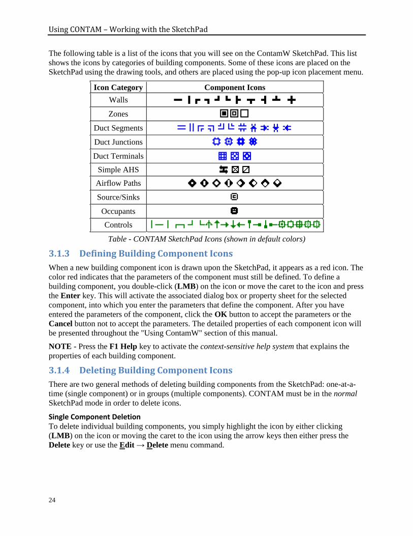
Using CONTAM – Working with the SketchPad
24
The following table is a list of the icons that you will see on the ContamW SketchPad. This list
shows the icons by categories of building components. Some of these icons are placed on the
SketchPad using the drawing tools, and others are placed using the pop-up icon placement menu.
Icon Category Component Icons
Walls
Zones
Duct Segments
Duct Junctions
Duct Terminals
Simple AHS
Airflow Paths
Source/Sinks
Occupants
Controls
Table - CONTAM SketchPad Icons (shown in default colors)
3.1.3 Defining Building Component Icons
When a new building component icon is drawn upon the SketchPad, it appears as a red icon. The
color red indicates that the parameters of the component must still be defined. To define a
building component, you double-click (LMB) on the icon or move the caret to the icon and press
the Enter key. This will activate the associated dialog box or property sheet for the selected
component, into which you enter the parameters that define the component. After you have
entered the parameters of the component, click the OK button to accept the parameters or the
Cancel button not to accept the parameters. The detailed properties of each component icon will
be presented throughout the "Using ContamW" section of this manual.
NOTE - Press the F1 Help key to activate the context-sensitive help system that explains the
properties of each building component.
3.1.4 Deleting Building Component Icons
There are two general methods of deleting building components from the SketchPad: one-at-a-
time (single component) or in groups (multiple components). CONTAM must be in the normal
SketchPad mode in order to delete icons.
Single Component Deletion To delete individual building components, you simply highlight the icon by either clicking
(LMB) on the icon or moving the caret to the icon using the arrow keys then either press the
Delete key or use the Edit → Delete menu command.
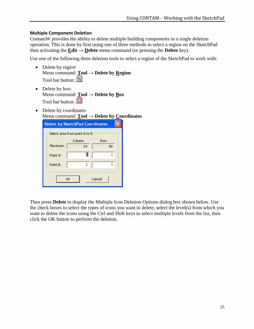
Using CONTAM – Working with the SketchPad
25
Multiple Component Deletion ContamW provides the ability to delete multiple building components in a single deletion
operation. This is done by first using one of three methods to select a region on the SketchPad
then activating the Edit → Delete menu command (or pressing the Delete key).
Use one of the following three deletion tools to select a region of the SketchPad to work with:
Delete by region
Menu command: Tool → Delete by Region
Tool bar button:
Delete by box:
Menu command: Tool → Delete by Box
Tool bar button:
Delete by coordinates
Menu command: Tool → Delete by Coordinates
Then press Delete to display the Multiple Icon Deletion Options dialog box shown below. Use
the check boxes to select the types of icons you want to delete, select the level(s) from which you
want to delete the icons using the Ctrl and Shift keys to select multiple levels from the list, then
click the OK button to perform the deletion.

Using CONTAM – Working with the SketchPad
26
Figure - Multiple Icon Deletion Options dialog box
NOTE: Some deletion operations will invalidate existing relationships between items in the
project file. This can lead to the inability of ContamW to save the project file and/or ContamX to
perform a simulation on the project file. For example, deleting a zone that is referenced by an
occupant schedule will prevent ContamW from saving the project file. However, an error
message will be provided to notify you when you attempt to save. For this reason, you should
always create a backup copy prior to performing major deletion operations.
Network Deletion (Ducts and Controls) You can delete a set of connected ducts or controls using a single command. Highlight any icon
within the network you wish to delete and select Edit → Delete Network from the menu or use
the Ctrl+Delete keyboard shortcut. If deleting a control network, you may be prompted whether
to delete or undefine phantom nodes that reference the network being deleted.
3.1.5 Find and Replace Building Component Data
ContamW provides the ability to perform both simple searches for building components and to
perform find-and-replace operations. Both features involve the use of a dialog box that can be
displayed simultaneously with the SketchPad to allow interaction between both the SketchPad
and the dialog boxes.
Find Use the Find feature to locate various building component icons on the SketchPad by either their
Number or Name properties. Be aware that numbers may change whenever the total number of
each type of component is modified by either adding or deleting components. Whenever the
project file is saved, the components will be renumbered based on their SketchPad position
starting from the top level and working from left to right then top to bottom on the SketchPad
down through the building levels.

Using CONTAM – Working with the SketchPad
27
Menu Command: Edit → Find…
Keyboard Shortcut: Ctrl+F
Figure – Find dialog box
Simply select the type of component icon you wish to locate, select either a number or name
from the lists provided and click the Find button. The icon will be located and highlighted on the
SketchPad. If there are no components of a given type, the search controls will be disabled.
Searchable items:
Air Handling Systems
Airflow Paths - including Supplies and Returns of Simple Air Handling Systems
Control Nodes - sub-nodes of super nodes will defer to the super node
Duct Junctions
Duct Segments
Occupants
Source/Sinks
Zones - including implicit supply and return zones of simple air handling systems
Find and Replace The Find and Replace feature consists of a more advanced find feature that enables you to
generate lists of items based on user-selected ranges of property values. You can then replace
parameters of the items in the list of items found.
Menu Command: Edit → Replace…
Keyboard Shortcut: Ctrl+R
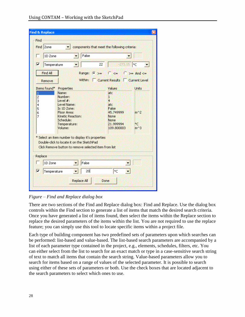
Using CONTAM – Working with the SketchPad
28
Figure – Find and Replace dialog box
There are two sections of the Find and Replace dialog box: Find and Replace. Use the dialog box
controls within the Find section to generate a list of items that match the desired search criteria.
Once you have generated a list of items found, then select the items within the Replace section to
replace the desired parameters of the items within the list. You are not required to use the replace
feature; you can simply use this tool to locate specific items within a project file.
Each type of building component has two predefined sets of parameters upon which searches can
be performed: list-based and value-based. The list-based search parameters are accompanied by a
list of each parameter type contained in the project, e.g., elements, schedules, filters, etc. You
can either select from the list to search for an exact match or type in a case-sensitive search string
of text to match all items that contain the search string. Value-based parameters allow you to
search for items based on a range of values of the selected parameter. It is possible to search
using either of these sets of parameters or both. Use the check boxes that are located adjacent to
the search parameters to select which ones to use.
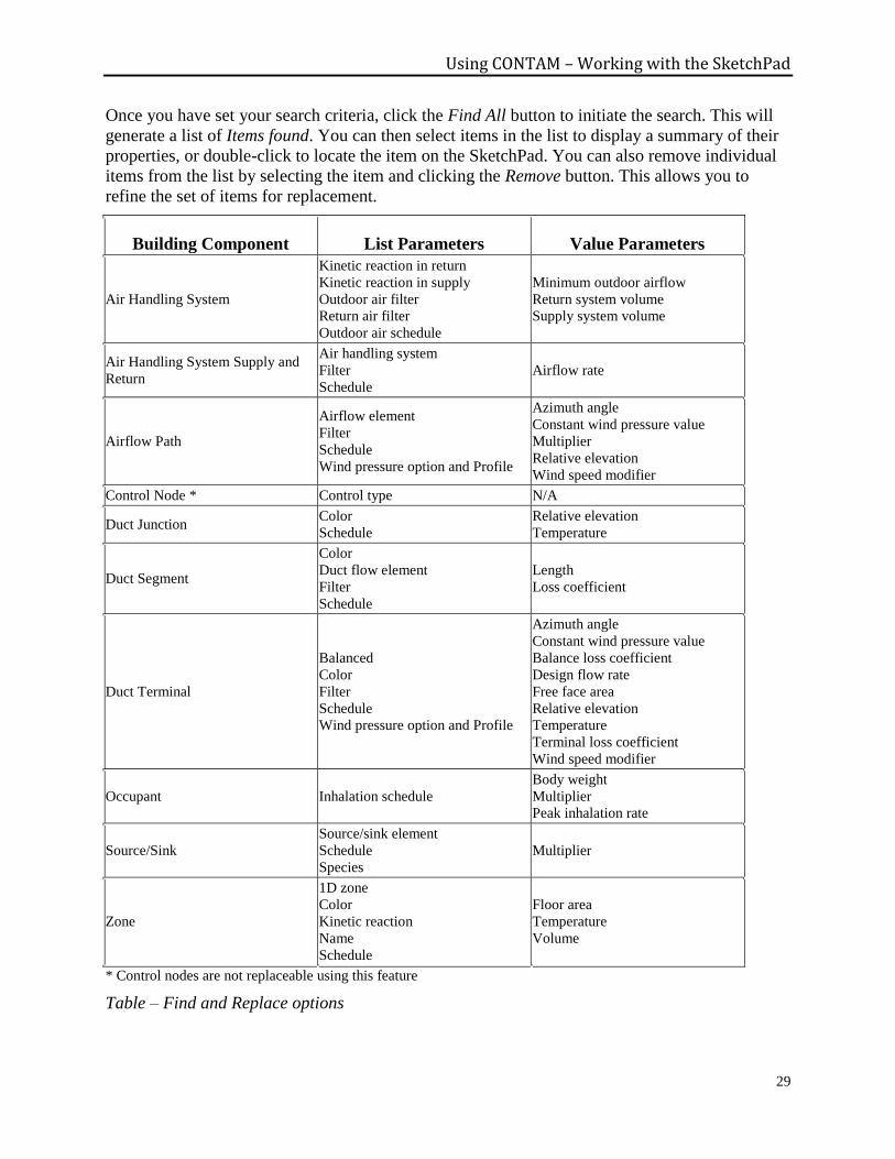
Using CONTAM – Working with the SketchPad
29
Once you have set your search criteria, click the Find All button to initiate the search. This will
generate a list of Items found. You can then select items in the list to display a summary of their
properties, or double-click to locate the item on the SketchPad. You can also remove individual
items from the list by selecting the item and clicking the Remove button. This allows you to
refine the set of items for replacement.
Building Component List Parameters Value Parameters
Air Handling System
Kinetic reaction in return
Kinetic reaction in supply
Outdoor air filter
Return air filter
Outdoor air schedule
Minimum outdoor airflow
Return system volume
Supply system volume
Air Handling System Supply and
Return
Air handling system
Filter
Schedule
Airflow rate
Airflow Path
Airflow element
Filter
Schedule
Wind pressure option and Profile
Azimuth angle
Constant wind pressure value
Multiplier
Relative elevation
Wind speed modifier
Control Node * Control type N/A
Duct Junction Color
Schedule
Relative elevation
Temperature
Duct Segment
Color
Duct flow element
Filter
Schedule
Length
Loss coefficient
Duct Terminal
Balanced
Color
Filter
Schedule
Wind pressure option and Profile
Azimuth angle
Constant wind pressure value
Balance loss coefficient
Design flow rate
Free face area
Relative elevation
Temperature
Terminal loss coefficient
Wind speed modifier
Occupant Inhalation schedule
Body weight
Multiplier
Peak inhalation rate
Source/Sink
Source/sink element
Schedule
Species
Multiplier
Zone
1D zone
Color
Kinetic reaction
Name
Schedule
Floor area
Temperature
Volume
* Control nodes are not replaceable using this feature
Table – Find and Replace options

Using CONTAM – Working with the SketchPad
30
3.1.6 Viewing Results on the SketchPad
ContamW provides some graphical displays of simulation results upon the SketchPad. You can
display airflow rates and pressure differences across airflow paths on the SketchPad if a
simulation has been performed and results of the simulation are available (see Viewing Results
in the Working with Results section of the manual).
3.1.7 Viewing Envelope Wind Pressure Differentials
ContamW provides a feature that allows you to visualize the effects of wind upon a building
envelope. A graphical display of wind pressures at each of the flow paths that are adjacent to the
ambient zone can be viewed on the SketchPad (see Checking Wind Pressure Data in the
Defining Steady State Weather and Wind section). This feature enables you to verify input of
wind speed and direction data with respect to the orientation of the building envelope to the
wind.
3.1.8 Working with Project Files
All information related to the layout, building components, and occupant information of your
CONTAM project are stored in a "project" file. When you save the project file, it will be stored
with the ".PRJ" extension. CONTAM project file names must conform to the file naming
conventions of the Windows operating system. This project name is displayed in the Title bar of
the ContamW application window.
All project file operations are contained under the File menu. These operations include: New
Project, Open Project…, Save Project, and Save Project As… Note that some of these file
operations have keyboard short-cuts and/or tool bar buttons associated with them.
Creating a New Project Menu Command: File → New Project
Keyboard Shortcut: None
Toolbar Button:
Use this command if you are currently working on a project and you wish to create a new one.
This command will clear the SketchPad and all data related to the current project from
ContamW's program memory. If your current project has not been saved prior to executing this
command, you will be asked whether or not you wish to save it prior to clearing it.
A dialog box will appear enabling you to enter a project description (See Editing the Project
File Description below )
Opening an Existing Project Menu Command: File → Open Project…
Keyboard Shortcut: Ctrl+O
Toolbar Button:
OR
Menu Command: File → Recent Projects
Use these menu items to open and existing CONTAM project file. This command will display
the File Open dialog box typical of Windows applications. This dialog box is set to display only

Using CONTAM – Working with the SketchPad
31
those files having the ".PRJ" extension in order to simplify your search for CONTAM project
files. Follow the typical procedure for opening a file using the Windows operating system.
The Open dialog box provides you with both the Version and Description of the highlighted
project file. You can edit the project file description via the File → Project Description… menu
item.
When a project file is successfully read by ContamW, a backup copy of the project file is created
with the name CONTAM.BKP in the program directory.
Opening Project Support Files You can now open input and output files related to the current project, including the ContamW
and ContamX log files, via the File → Open Project Input Files and File → Open Project
Output Files menu commands. The files will open according to the Windows file extension
associations.
Converting Projects from Previous Versions Menu Command: File → Open Project…
Keyboard Shortcut: Ctrl+O
This is the same as opening an existing project. However, after you open a project of an earlier
version it will be untitled, so you must give the project a name when saving it. Once you save a
project with the most recent format, you will no longer be able to open it using an earlier version
of CONTAM.
A utility is also provided on the NIST website that will enable you to quickly update a set of
project files to the current version. For example PrjUp24.exe will upgrade to the CONTAM 2.4
format. To utilize this utility, copy prjup24.exe and the desired project file(s) to a new directory,
select the projects to update and drag and drop them onto the prjup24.exe file. This will replace
the existing files with updated versions.
Editing the Project File Description Menu Command: File → Project Description…
Use this feature to enter a project file description which is provided to help you manage your
project files. This description will be available when you are opening project files from within
ContamW.
Saving a Project Menu Command: File → Save Project
Keyboard Shortcut: Ctrl+S
Toolbar Button:
This option saves the building description to the project file under its current name.
Renaming a Project Menu Command: File → Save Project As…
Keyboard Shortcut: None
Toolbar Button: None
Use this command to save a copy of the current project file under a new name. This will display
the Windows "Save As" dialog box and allow you to specify both a storage location and a file
name for the project file. ContamW will automatically append the ".prj" extension to the
Using CONTAM – Working with the SketchPad
32
filename, so you do not have to give the file an extension. If you do give the file an extension,
".prj" will be appended as well as the extension you provide. If you specify the name of an
existing file, you will be warned that saving the file will overwrite the existing file. If you try to
save an untitled or new project file prior to giving it a name, the "Save As" dialog box will be
displayed.
Exiting ContamW Menu Command: File → Exit
Keyboard Shortcut: None
Toolbar Button: None
You can also exit the program using the standard window-closing button located in the upper
right-hand corner of the program window.
Using CONTAM – Configuring ContamW
33
3.2 CONFIGURING CONTAMW
The Program and Project options of ContamW are available from the View menu. Program
options can be saved to the CONTAM.CFG file located in the CONTAM Program Directory.
Upon startup, ContamW looks for this file and loads the saved settings if the file exists. This way
you can set ContamW to start with the same default settings each time you run the program.
Project options are saved with the current project file.
NOTE: The path name of the EWC-to-WPC file converter does not appear in the configuration
dialog boxes; however, if a converter is selected when you click the Save button it will be saved
to the CONTAM.CFG file. The value saved will be that which you have set in the WPC File…
selection of the Weather menu. To reset the converter name back to "null," you must edit the
configuration file manually.
3.2.1 Project Configuration Properties
All of these settings are saved within the CONTAM project file.
Units
The following parameters define the units and temperature that will be used by default
throughout the project when you are providing input to the program. You do not have to use
these units throughout the project; however, you should select the primary set of units for
convenience when entering data throughout a project. You can change these defaults at any time
while working with a project, and you can select different units for individual parameters as you
enter them.
System of Units: You can select the appropriate radio button to set the system of units that
you would like the program to use. You can either select the International System of Units
(SI) or the Inch-Pound (IP) system of units.
Units of Flow: You can select the appropriate radio button for the most commonly used units
of flow in the current project. These are the units in which airflow simulation results will be
displayed within the status bar. ContamW converts all airflow rates to and performs all
calculations in mass flow units of kg/s. Note that all volumetric airflow rate units are at
standard temperature and pressure.
Default Zone and Junction Temperature: This value will be the default temperature used
whenever you create a new zone, duct junction or terminal within the current project. If you
change this value, you will be prompted as to whether or not you would like to update the
temperatures of all existing zones, junctions and terminals.
SketchPad Dimensions
Size: This is the width and height of the SketchPad. These dimensions are presented in both
cell units and units of length as defined by the Scaling Factor below. The SketchPad is made
up of square cells that represent each space wherein an icon may be placed. The default (and
minimum) values are 66 cells wide and 58 cells high.
Scaling Factor: Sets the dimension of a cell in order to calculate SketchPad locations and
wall dimensions in the units provided when displaying pseudo-geometry on the SketchPad.
Using CONTAM – Configuring ContamW
34
Show Pseudo-Geometry: The pseudo-geometry drawing mode uses the Scaling Factor to
present location and wall dimensions on the SketchPad in the Status Bar. This feature can be
useful when working with the TRNSYS-CONTAM coupling capability that requires
geometrical data for the TRNSYS building representation used by TRNSYS Type56.
Pseudo-geometry can also be useful when setting airflow path multipliers because wall areas
can be displayed. The extents of items (dx and dy) will be displayed in the Status Bar as you
draw them.
Origin: Sets the location (column and row) of the origin to be used when calculating the
position of items on the SketchPad. A special icon will appear on the SketchPad at the
specified location. By default the origin represents the bottom-left of the SketchPad grid
(column 1, row 56) and y-values are positive above the origin. You can invert the y-axis so
that y-values are negative above the origin.
NOTE: You can also set the origin by right-clicking on the SketchPad and selecting "Set
Origin" from the context menu.
3.2.2 Program Configuration Properties
Use the Save button at the bottom of this dialog box to save the CONTAM.CFG file.
Units
The Program units define the units and temperature that will used to populate the Project units
(presented above) when you create a new project file.
SketchPad Display
Show Floating Status: Check this box to display the Floating Status box on the SketchPad.
You can also turn the floating status box on and off via the View → Floating Status (Ctrl+T)
menu command.
Show Zone Colors: Check this box to display zone fill colors on the SketchPad. If this box
is not checked, then all zones will be filled using the "Background" palette color. You can
also turn the color zones option on and off via the View → Color Zones (Ctrl+Z) menu
command.
Show Duct Colors: Check this box to display duct colors on the SketchPad. If this box is not
checked, then all ducts will be displayed using the "Ducts" palette color. You can also turn
the color ducts option on and off via the View → ColorZones (Ctrl+Z) menu command.
Maximize ContamW at startup: Check this box to maximize the ContamW window when
the you start the program.
Cell/Icon Size
Current Cell/Icon Size: There are seven options for displaying icons on the SketchPad (1x1,
2x2, 3x3, 4x4, 5x5, 8x8, and 16x16). The default option is 8x8. This is a "zooming" feature
that provides a visual aid to enable you to view sketches in more detail or to fit larger
sketches within the program window. The cell size has no effect on the project simulation.
There are two "zooming" buttons provided on the toolbar to quickly increase and decrease
the cell size according to the available cell sizes below.
Using CONTAM – Configuring ContamW
35
Available Cell Sizes: Use these check boxes to select which sizes you want available. The
1x1 size causes problems with some versions of the Window 98 operating system. If this is
the case for you, then deselect the 1x1 check box and click the "Save Configuration" button.
Cell Jump: Use this to set the number of SketchPad cells the cursor will jump when you use
the Shift + Arrow Keys to maneuver around the SketchPad.
Colors
Palettes: ContamW provides the ability to modify the color of items displayed on the
SketchPad. You can select one of four available palettes. You can not modify the colors of
the "Default" palette, but you can modify the other three "User Palettes." Select a palette to
display the colors of the palette in the Palette Colors section below.
Palette Colors: These are the colors use to display items on the SketchPad. Click the color
box to change the color used to display each type of item. Only the colors of the User
Palettes can be changed. The following is a brief description of each category.
Foreground - Defined icons including walls
Background - Background of SketchPad cells, default zone fill and fill of all zones when
Color Zones option is not active.
Flow Results - Lines displaying scaled flow results for airflow paths and duct terminals
Pres Results - Lines displaying scaled pressure difference results across airflow paths in
the Results and Wind Pressure view modes
Drawing Line - Cell highlight when drawing on the SketchPad
Undefined - Undefined icons
Controls - Defined control icons
Ducts - Default color of defined ducts and color of all defined ducts when Color Ducts
view option is not active
Errors - Background color of cells when an error condition is being highlighted on the
SketchPad. Errors are indicated when a building check fails. Building checks are
performed when you choose Run Simulation or Create ContamX Input File from the
Simulation menu.
Cursor - SketchPad drawing and icon selection cursor
Highlight - Icon highlighting color for find operation
Sub Level - All icons on sub-level when sub-level display option is activated via the
Level → Reveal Level Below (Ctrl+Shift+B) menu command.
Results Display
Results Lines: You can select whether or not to display the airflow rates and pressure
differences across airflow paths on the SketchPad when in the Results Display Mode.
Both Pressure and Flow: Display both the airflow rates (green lines) and pressure
differences (red lines).
Pressure Only: Display only the pressure difference lines.
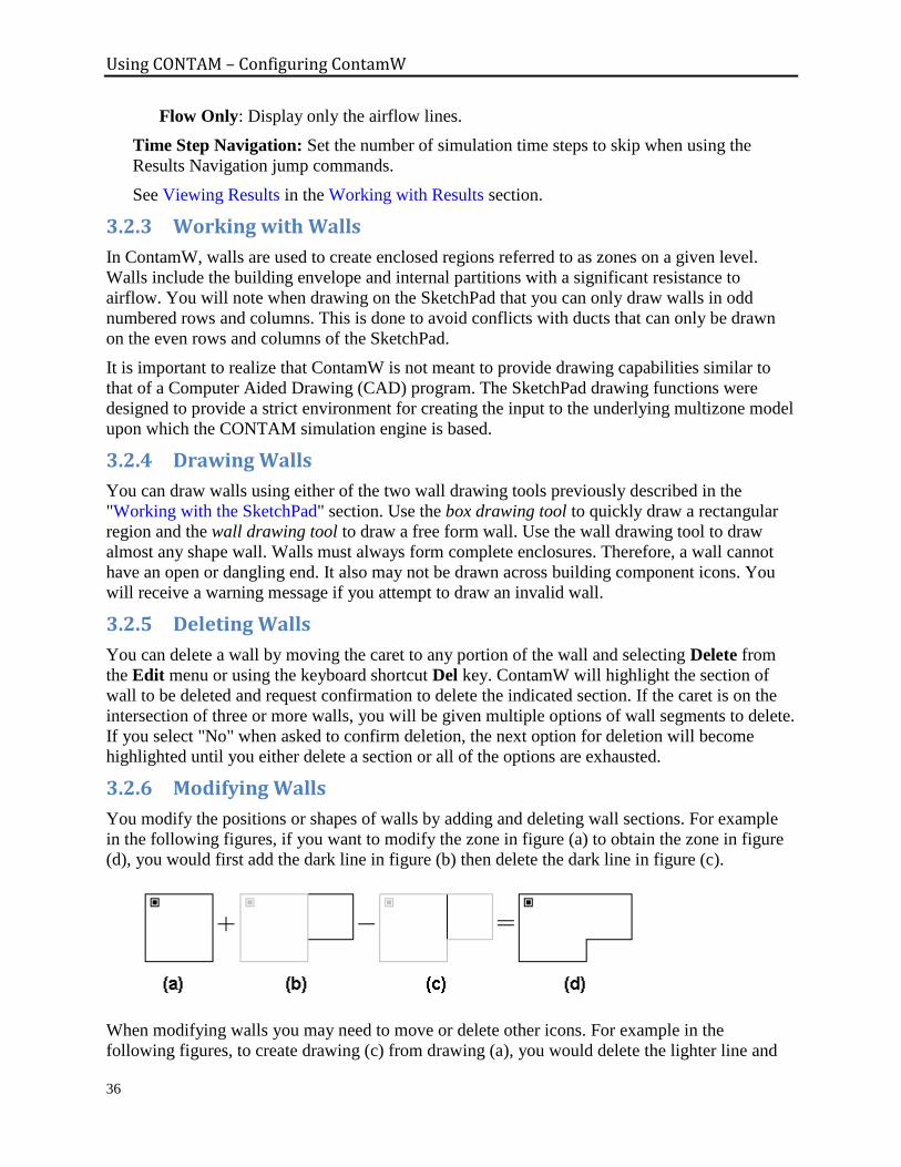
Using CONTAM – Configuring ContamW
36
Flow Only: Display only the airflow lines.
Time Step Navigation: Set the number of simulation time steps to skip when using the
Results Navigation jump commands.
See Viewing Results in the Working with Results section.
3.2.3 Working with Walls
In ContamW, walls are used to create enclosed regions referred to as zones on a given level.
Walls include the building envelope and internal partitions with a significant resistance to
airflow. You will note when drawing on the SketchPad that you can only draw walls in odd
numbered rows and columns. This is done to avoid conflicts with ducts that can only be drawn
on the even rows and columns of the SketchPad.
It is important to realize that ContamW is not meant to provide drawing capabilities similar to
that of a Computer Aided Drawing (CAD) program. The SketchPad drawing functions were
designed to provide a strict environment for creating the input to the underlying multizone model
upon which the CONTAM simulation engine is based.
3.2.4 Drawing Walls
You can draw walls using either of the two wall drawing tools previously described in the
"Working with the SketchPad" section. Use the box drawing tool to quickly draw a rectangular
region and the wall drawing tool to draw a free form wall. Use the wall drawing tool to draw
almost any shape wall. Walls must always form complete enclosures. Therefore, a wall cannot
have an open or dangling end. It also may not be drawn across building component icons. You
will receive a warning message if you attempt to draw an invalid wall.
3.2.5 Deleting Walls
You can delete a wall by moving the caret to any portion of the wall and selecting Delete from
the Edit menu or using the keyboard shortcut Del key. ContamW will highlight the section of
wall to be deleted and request confirmation to delete the indicated section. If the caret is on the
intersection of three or more walls, you will be given multiple options of wall segments to delete.
If you select "No" when asked to confirm deletion, the next option for deletion will become
highlighted until you either delete a section or all of the options are exhausted.
3.2.6 Modifying Walls
You modify the positions or shapes of walls by adding and deleting wall sections. For example
in the following figures, if you want to modify the zone in figure (a) to obtain the zone in figure
(d), you would first add the dark line in figure (b) then delete the dark line in figure (c).
When modifying walls you may need to move or delete other icons. For example in the
following figures, to create drawing (c) from drawing (a), you would delete the lighter line and
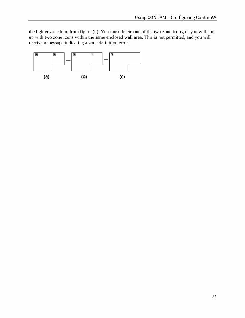
Using CONTAM – Configuring ContamW
37
the lighter zone icon from figure (b). You must delete one of the two zone icons, or you will end
up with two zone icons within the same enclosed wall area. This is not permitted, and you will
receive a message indicating a zone definition error.
Using CONTAM – Working with Levels
38
3.3 WORKING WITH LEVELS
CONTAM projects are organized by levels. Each level of a CONTAM project contains a plan
view drawing. Typically, each level of a CONTAM project corresponds to a floor of a building.
Depending on the detail required for your modeling purposes, you could represent a building
floor using multiple levels. For example, a level could be used to represent a ceiling or floor
plenum.
3.3.1 Creating Levels
When you first start ContamW, a default level is created so that you can begin working on a
drawing right away without having to create a new level. There are three commands in the Level
menu that you use when creating new levels. These are the Copy Level, Paste Level, and Insert
Blank Level commands. Whenever you create a new level, whether it is blank or a copy of
another level, ContamW will give it a default name that will consist of a number enclosed within
the "<" and ">" characters. You can modify this name later by editing the data associated with a
level.
You must be careful when copying levels within ContamW. For example, you might have an air
handler defined within a duct system on a level and then copy it to another level. This would
create another air handler on the new level. If the ductwork is connected between the two levels,
the two air handlers may act against each other. You must be careful to make connections
between building levels in a manner that makes sense for your purposes.
Creating Blank Levels Menu Command: Level → Insert Blank Level (Above/Below Current Level)
Keyboard Shortcut: None
Toolbar Button: None
Use these commands to create a blank level. When you create a blank level, you must select
whether you want it created above or below the current level.
Copying and Pasting levels Menu Command: Level → Copy Level along with
Level → Paste Level (Above/Below Current Level)
Keyboard Shortcut: None
Toolbar Button: None
With ContamW you can copy an entire level and insert it as an entire level anywhere within the
current project. Use the Copy Level command to copy the level currently displayed on the
SketchPad; move to either the level above or below where you wish to insert the copied level and
use one of the Paste Level commands to insert the copied level.
3.3.2 Viewing Levels
If a project has more than one level, you can specify the level that you want to view or modify on
the SketchPad by using the level commands. All level-related commands are located under the
Level menu. There are also some shortcut keys and toolbar buttons provided for your
convenience.

Using CONTAM – Working with Levels
39
Moving Up/Down a Level Menu Command: Level → Go to (Level Above/Below)
Keyboard Shortcut: Page Up, Page Down
Toolbar Button:
Use this command to change which level you want the SketchPad to display.
Changing the Currently Active Level Menu Command: Level → Go to (Level Above/Below)
Keyboard Shortcut: Page Up, Page Down
Toolbar Button:
Use this command to change which level you want the SketchPad to display.
Displaying Multiple Levels Menu Command: Level → Reveal Level Below
Keyboard Shortcut: Ctrl+Shift+B
Toolbar Button: None
Use this command to see both the current level and the level below the current level at the same
time. ContamW will display the walls and building component icons of the level below in gray.
This feature is useful for aligning building features between adjacent levels.
3.3.3 Deleting Levels
Menu Command: Level → Delete Level
Keyboard Shortcut: None
Toolbar Button: None
Use this command to delete an entire level. Once you have deleted a level, you cannot undo the
deletion. You may want to save a copy of the file prior to deleting a level; this is the only way to
prevent losing your work.
3.3.4 Modifying Levels
To modify level data, you access the Level Data dialog box using the Edit Level Data…
command of the Level menu. You can also use the keyboard shortcut F8 to display the dialog
box. The following section shows the information contained on the "Level Data" dialog box.
3.3.5 Level Data
This is the information associated with each level that you create. ContamW will provide default
values for this data, but you can modify it as required for your particular building.
Name: Name to identify the level. All level names must be unique.
Elevation of this level: The elevation of the base of the level above ground.
Distance to level above: This is the height of the level from floor to ceiling. ContamW will use
this value to calculate zone volumes based on the floor area of each zone. If you change this
value, a dialog box will appear asking if you would like ContamW to adjust the volumes of the
zones on the level based on the new level height. If you select Yes, then the zone volumes will
Using CONTAM – Working with Levels
40
be adjusted by Vnew = Vold * Hnew / Hold. If there are phantom zones on the level, you will be
advised that their volumes were not adjusted, so you should handle those zones individually.
3.3.6 Checking Levels
Menu Command: Level → Check Current Level
Keyboard Shortcut: None
Toolbar Button: None
Use this feature to check the data for the currently displayed level and make sure the building
components are defined. Errors will be highlighted in red on the SketchPad.

Using CONTAM – Working with Zones
41
3.4 WORKING WITH ZONES
A zone is a volume of air separated from other volumes of air by walls, floor and ceiling.
Generally, zones are characterized by having a uniform temperature and pressure (that varies
hydrostatically) and contaminant concentration. However, the concentration within user-selected
zones can be allowed to vary in one dimension (See 1D Zone Data Properties within this section)
via the 1D convection/diffusion model (See the Theoretical Background section). In addition,
there are three different types of zone icons: normal, phantom and ambient. A normal zone icon
represents a zone that is separated by a floor from the zone below. A phantom zone is used to
indicate that there is no floor below the enclosed region on a given level. That is, the region on
this level is actually part of the zone below and has the same temperature and contaminant
concentration. An ambient zone icon represents the outdoor air. The ambient zone, which
surrounds the building, is already identified by default by the icon at the upper-left corner of the
SketchPad.
You create zones on the SketchPad by first drawing walls that enclose a region, placing a single
zone icon within the enclosed region, and then defining the zone icon. Eventually, every zone
must be connected to either the ambient zone or a constant pressure zone either directly or
indirectly via any set of paths that prevents the zone from being isolated from a zone of "known"
pressure.
3.4.1 Creating Zones
You create zones by drawing walls upon the SketchPad. The wall drawing operations are
described in the Drawing Walls section of this manual. The shape and size of zones as drawn
upon the SketchPad do not provide the underlying model with any scaling information.
However, the manner in which the enclosed regions border each other is significant. Any zones
between which you wish to provide a direct connection (via an airflow path) must share a
common wall. Therefore, when drawing a building floor plan, you should try to maintain the
general topology of the actual floor plan. While scale is not significant, ContamW does provide
you with the SketchPad coordinates that may help you when laying out your project.
The dimensions of your zones are determined when you define them. If you change the shape or
size of a region on the SketchPad that contains a zone icon, the dimensions do not change
according to the model unless you actually modify the properties of the associated zone icon.
3.4.2 Deleting Zones
You delete a zone by first deleting the zone icon. After you delete the zone icon, delete the wall
or walls necessary to eliminate the enclosed region that is left behind. You must avoid the
existence of an enclosed region without a zone icon; CONTAM will not perform a simulation
with an undefined zone icon in a project.
3.4.3 Modifying Zones
You modify the SketchPad representation of a zone by adding and removing walls. This
procedure is described in the Modifying Walls section of this manual. To modify the parameters
of a zone, you use the icon definition procedure (See Defining Building Component Icons) to
display its properties and make the desired changes.
Using CONTAM – Working with Zones
42
Once you define a zone, you can move the zone icon anywhere within the zone using the Cut
and Paste functions of the Edit menu. These commands will only allow you to paste the icon
into the zone in which it is currently located.
3.4.4 Defining Zones
After you draw the enclosed region of a zone, you must define the zone. To define a zone you
must first draw a zone icon within the enclosed region (See Drawing Building Component Icons)
and then use the icon definition procedure (See Defining Building Component Icons) to display
and edit the properties of the zone.
The properties of each zone include a name, temperature (constant or scheduled), pressure
(variable or constant), volume, information describing contaminant behavior within the zone, and
1D zone information. You must provide each zone with a name that is unique to each level of a
project. For this reason, you cannot copy zone data within a level. However, you can copy entire
levels of data, including zone data, from one level to another (See Creating Levels). Detailed
descriptions of zone properties are given under Zone Properties below.
Only normal zones require definition. Ambient and phantom zone icons appear as defined icons
as soon as you place them onto the SketchPad. However, you must include the volume of
phantom zones in the volume of the associated normal zone below it.
3.4.5 Zone Properties
This section provides detailed descriptions of the specific zone properties. The following
sections are the context-sensitive help topics that you can access by pressing F1 when working
with property pages of the "Zone Properties" property sheet.
Zone – Zone Data Properties
These are the basic properties that describe a zone.
Zone Name: This is the symbolic name of the zone. Enter a name up to 15 characters in length.
Zone names must be unique within each level of a building.
Dimensions
Volume: Zone volume is used in the dynamic contaminant calculations. For phantom zones,
the zone volume is set at the standard zone icon on the lowest level for the entire height of
the zone and includes the volume of the phantom zones on the levels above.
Floor Area: Instead of the volume, you may enter a floor area. Floor area is then multiplied
by the height of the current building level to compute a volume. This area is not used for any
other purpose by CONTAM.
Color: Select a zone fill color to help you distinguish zones on the SketchPad. You must
activate the Color Zones option from the View menu in order to display zone colors on the
SketchPad.
Include in Building Volume: This refers to the calculation of whole building air change
rates that you can now have CONTAM perform during simulation. The associated check box
is checked by default, so if you do not want the zone to be included in the whole building
volume you should uncheck this box. The air change rate and building pressurization
calculations will calculate the total rate of airflow from ambient into all of the zones having
Using CONTAM – Working with Zones
43
this box checked. Typically, you would include all conditioned space in the building volume;
for example, you might not want to include an attic or crawl space.
Temperature & Pressure
Temperature: Set the value you want to use as the constant temperature of the zone.
Whenever you create a new zone, ContamW will use the default value, which you can
override by entering another value. You can set the default zone temperature via the
Options… command of the View menu. Optionally, you can define a Schedule for the zone
temperature via the Schedule properties (See Schedule Properties for zone temperature).
Pressure: The zone air pressure relative to ambient can be specified as either variable or
constant. Typically you would set the zone pressure to be variable and allow it to be
calculated during the simulation. However, you might set the pressure to be constant if you
want to simulate a fan pressurization (blower door) test of a building (see Building
Pressurization Test in the Applications section of the manual) or to perform analytic test
cases of CONTAM.
Zone – Contaminant Properties
These are the contaminant-related properties of a zone. Contaminants must be defined prior to
defining contaminant data for a zone. To define contaminants, select Data then Contaminants…
from the main program menu.
Zone Name: This is the symbolic name of the zone as entered on the Zone Data property page.
Contaminant Concentrations: Select variable or constant. Typically you would set this to
variable and allow ContamX to calculate the contaminant concentration within the zone during
simulation. However, you may wish to set this to constant as a simple means of creating a simple
contaminant source within a zone. If you set this to constant, the contaminant concentrations in
this zone will begin and remain at the values you set for the initial concentrations.
Initial Concentration: Select a contaminant from the list and enter the initial contaminant
concentrations for dynamic (transient) simulations. Note that only those species you’ve selected
to be contaminants (to use during simulation) appear in the list. If a species for which you wish
to set an initial concentration does not appear in the list you must set "Use in simulation"
property of the corresponding species to be true (See Creating Species and Contaminants). You
can reset these initial values through the Run Control Properties of the Simulation Parameters.
IMPORTANT: Changing the number of contaminants, i.e. those species used in the simulation,
will reset the initial concentrations of all zones to the default contaminant concentrations. You
can reset all of these concentrations via the Run Control Properties as indicated above or
individually here.
Sum of Non-trace Initial Concentrations: This value is provided as a check for you to insure
that you input a reasonable set of initial values when using non-trace contaminants. This value
should be very close to 1.0.
Kinetic Reactions: If there are previously defined kinetic reactions within the current project,
you may select one from the list of names. Click the "New Reaction" button to define a new
kinetic reaction. To view or modify existing kinetic reaction data click the "Edit Reaction"
button. Setting this field to <none> indicates no reactions in the zone. You can also import
kinetic reactions from a contaminant-related library file (See Working with Data and Libraries).
Using CONTAM – Working with Zones
44
Zone – Detailed Zone Properties
These are the properties used to define 1D convection/diffusion zones, in which contaminant
concentrations can vary along a user-specified axis. This option is provided for cases in which
you need to account for the delay in contaminant transport within long or tall zones. If this
feature is enabled, ContamX will subdivide this zone along the specified axis into multiple cells
or sub-nodes for the purposes of contaminant transport calculations.
Zone Name: This is the symbolic name of the zone as entered on the Zone Data property page.
Zone Type
Normal Zone: well-mixed zone
1D Zone: 1D convection/diffusion zone
CFD Zone: Only one CFD zone is allowed per CONTAM project. Use the CFD0 Editor
(available via the NIST IAQanalysis website) to define the CFD properties of the zone,
e.g., zone mesh and boundaries.
1D Zone Data
Axial Dispersion Coef: Enter the axial dispersion coefficient and units for the zone. Note
that the zone dispersion coefficient is zone specific and is not necessarily the molecular
diffusion properties of the defined contaminants. This coefficient is empirically based and
should account for turbulent mixing as well.
Axis End Point Coordinates: Define the end points, Point 1 and Point 2, of the axis of the
1D zone. These coordinates will define the direction along which contaminant transport will
be calculated when treating this zone as a 1D convection diffusion zone. These values are
required to establish the relationship of other building components with respect to this zone,
i.e., flow paths, duct junctions and terminals, simple air-handling unit supply and return
points, contaminant source/sinks, sensors and occupants.
While the coordinate system is user-defined, ContamW will verify the relationship of 1D
zones to associated building components prior to running a simulation to insure that the
coordinates "match up." This verification is performed automatically when you select either
the Run Simulation or Create a ContamX Input File command from the Simulation
menu. If there are discrepancies, messages will be displayed notifying you of the nature of
the discrepancies.
X and Y: The X and Y values are in absolute coordinates. These values can be based on
scale drawings and/or a user-defined coordinate system. Unlike walls on the SketchPad,
axes are not required to be rectilinear, i.e., you may specify axes that are not horizontal or
vertical in the x-y plane.
Rel Elevation: Enter the Z-coordinate as the height relative to the base of the zone.
Cell Size: This is the cell size into which ContamX will sub-divide the zone during
simulation if the zone is to be treated as a 1D convection/diffusion zone. If the axis length
is not evenly divisible by the cell size, then the cell size will be adjusted as needed. While
there is no strict guidance on the selection of cell size, it should generally be on the order
of the flow velocity along the axis times the simulation time step.

Using CONTAM – Working with Zones
45
Units: Set the units of the above items.
Axis Orientation on the SketchPad: The orientation of the axis on the SketchPad is useful
when using a results viewing tool such as ContamRV. ContamRV can display the variation
of concentration within 1D zones if the simulation output options are set to write to the 1D
results files (See Simulation - Output Properties in the Simulation Parameters section). Mass
fractions of 1D zone cells are written to the 1D results file in the order from Point 1 to Point
2 of the Axis End Points. The "Axis Orientation" enables ContamRV to color the rectilinear
region of the zone on the SketchPad even if the axis endpoints specify an axis that is not
actually horizontal or vertical in the plan view, e.g., a slanted hallway.
CFD Zone Data
CFD Zone ID: This identifier is used to name the CFD files associated with this project.
These files will be generated by the CFD0 Editor and ContamX. For example, using the
CFD0 Editor you import a PRJ file that contains a CFD Zone. Once you have used the CFD0
Editor to define the CFD domain, you will use the CFD0 Editor to generate a CFD file
having the same name as the PRJ file but with the CFD Zone ID appended to it, e.g.,
MyProject_CfdZone.cfd. Running a coupled simulation will generate more similarly named
files having various extensions.
Zone – Schedule Properties
These are the properties used to define a temperature schedule for the zone. If a temperature
schedule is associated with the zone then the constant value will be overridden and the
simulation run control should be set to vary the density within building zones during simulation
(See Airflow Numerics Properties in the Working with Simulations section).
Zone Name: This is the symbolic name of the zone as entered on the Zone Data property page.
Temperature Schedule: Select the temperature schedule you want to associate with this zone.
(See Working with Schedules).
CVF/DVF Control: Values from either a CVF or DVF file can be used in place of the above
Schedule (read about CVF and DVF controls in the Control Element Types section). This
enables using these control element types without having to draw/define an associated control
network. The associated radio buttons "Use Neither", "Use CVF" and "Use DVF" are used to
select the desired control method. Select the heading name from the associated "Name" drop
down box that will display the headings of either the CVF or DVF file as per the aforementioned
radio button selection.
Control Status: This will display the current method of control: Schedule, direct CVF, direct
DVF or Control Network. If an actuator of a control network on the SketchPad is associated with
the scheduled item then it will take precedence over the Schedule and CVF/DVF Control. If
either the "Use CVF" or "Use DVF" radio button is selected then CVF or DVF will take
precedence over an associated schedule.
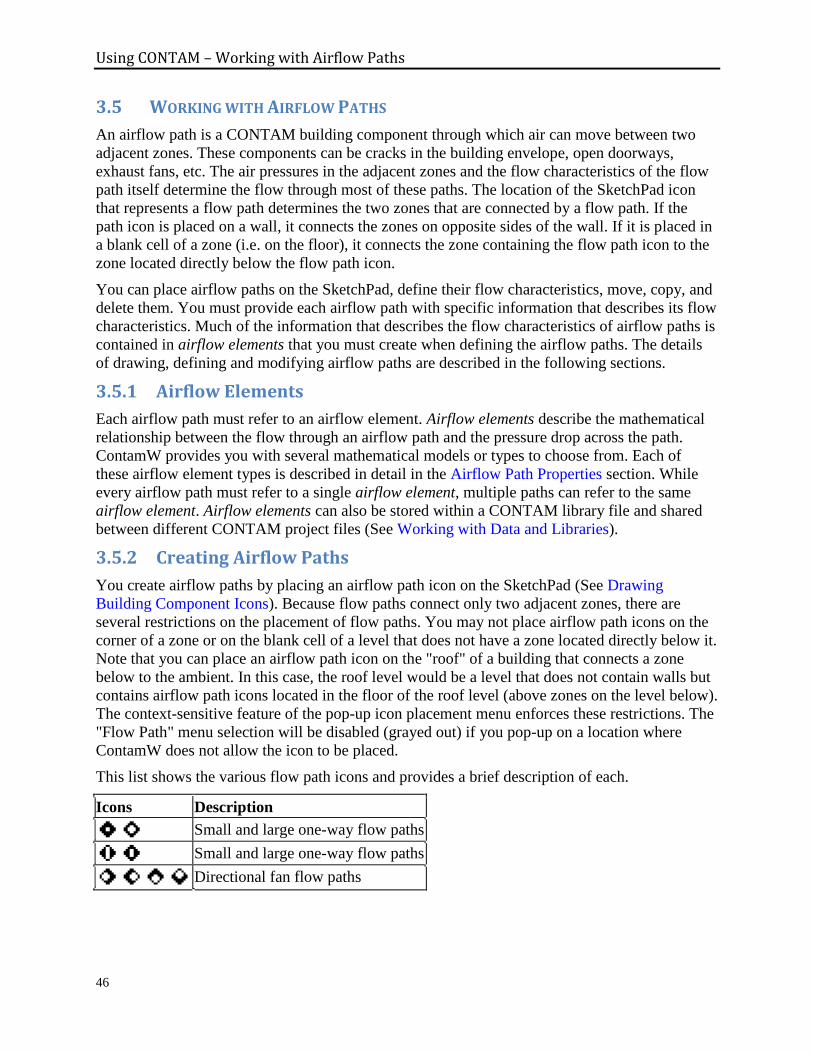
Using CONTAM – Working with Airflow Paths
46
3.5 WORKING WITH AIRFLOW PATHS
An airflow path is a CONTAM building component through which air can move between two
adjacent zones. These components can be cracks in the building envelope, open doorways,
exhaust fans, etc. The air pressures in the adjacent zones and the flow characteristics of the flow
path itself determine the flow through most of these paths. The location of the SketchPad icon
that represents a flow path determines the two zones that are connected by a flow path. If the
path icon is placed on a wall, it connects the zones on opposite sides of the wall. If it is placed in
a blank cell of a zone (i.e. on the floor), it connects the zone containing the flow path icon to the
zone located directly below the flow path icon.
You can place airflow paths on the SketchPad, define their flow characteristics, move, copy, and
delete them. You must provide each airflow path with specific information that describes its flow
characteristics. Much of the information that describes the flow characteristics of airflow paths is
contained in airflow elements that you must create when defining the airflow paths. The details
of drawing, defining and modifying airflow paths are described in the following sections.
3.5.1 Airflow Elements
Each airflow path must refer to an airflow element. Airflow elements describe the mathematical
relationship between the flow through an airflow path and the pressure drop across the path.
ContamW provides you with several mathematical models or types to choose from. Each of
these airflow element types is described in detail in the Airflow Path Properties section. While
every airflow path must refer to a single airflow element, multiple paths can refer to the same
airflow element. Airflow elements can also be stored within a CONTAM library file and shared
between different CONTAM project files (See Working with Data and Libraries).
3.5.2 Creating Airflow Paths
You create airflow paths by placing an airflow path icon on the SketchPad (See Drawing
Building Component Icons). Because flow paths connect only two adjacent zones, there are
several restrictions on the placement of flow paths. You may not place airflow path icons on the
corner of a zone or on the blank cell of a level that does not have a zone located directly below it.
Note that you can place an airflow path icon on the "roof" of a building that connects a zone
below to the ambient. In this case, the roof level would be a level that does not contain walls but
contains airflow path icons located in the floor of the roof level (above zones on the level below).
The context-sensitive feature of the pop-up icon placement menu enforces these restrictions. The
"Flow Path" menu selection will be disabled (grayed out) if you pop-up on a location where
ContamW does not allow the icon to be placed.
This list shows the various flow path icons and provides a brief description of each.
Icons Description
Small and large one-way flow paths
Small and large one-way flow paths
Directional fan flow paths
Using CONTAM – Working with Airflow Paths
47
3.5.3 Deleting Airflow Paths
You delete airflow path icons using the icon deletion procedure (See Deleting Building
Component Icons). Deleting airflow path icons from the SketchPad does not delete any airflow
elements that you may have defined. These flow elements can only be deleted using the
CONTAM Library Manager, accessible through the Data menu for each type of data element.
3.5.4 Modifying Airflow Paths
To modify the parameters of an airflow path, you use the icon definition procedure (See Defining
Building Component Icons) to display its properties and make the desired changes. You can also
move and copy airflow paths.
Moving Airflow Path Icons Once you define an airflow path, you can move the path icon using the Cut and Paste functions
of the Edit menu. ContamW will constrain the movement of path icons according to the
following rules. You can only move a flow path through a wall onto a wall, not onto the floor of
a zone. You can only move a flow path through a floor to another location on the floor, not onto
a wall. You can only move a path icon within the same level upon which it is located.
Copying Airflow Path Icons Once you define an airflow path, you can copy the path icon using the Copy and Paste functions
of the Edit menu. ContamW will constrain the copying of path icons according to the following
rules. You can only copy a flow path through a wall onto a wall, not onto the floor of a zone.
You can only copy a flow path through a floor to another location on the floor, not onto a wall.
You may copy a path icon from one level to another.
3.5.5 Defining Airflow Paths
After you draw a Flow Path icon on the SketchPad you must define it using the icon definition
procedure (See Defining Building Component Icons) to display and edit the properties of the
airflow path. This will display the "Airflow Path Properties" property sheet. Detailed
descriptions of all airflow path properties are given in the Airflow Path Properties section of this
manual. Once you have defined the properties of an airflow path, the icon will be displayed in
black. The icon representing the defined airflow path may be slightly different from the original
undefined icon depending on the type of airflow element you associate with the path (See the list
below). From now on, you use this icon to access the properties of the airflow path.
Some of the properties associated with an airflow path are optional: contaminant filtration,
schedule, wind pressure and pressure limit. You can associate contaminant filters with any flow
path, and you can define a filter for each contaminant contained in your CONTAM project. A
filter could be used, for example, to simulate the penetration of particles through a wall cavity.
You can use a schedule to vary the flow through a path as a function of time. For example, you
could use a schedule to open and close a path that represents a window. CONTAM allows you to
account for the direct effects of wind pressure on the envelope of a building. The envelope is
considered to be any wall that is adjacent to the ambient zone. If an airflow path is directly
connected to the ambient zone, a "Wind Pressure" property page will be displayed to allow you
to account for the effects of wind pressure on the path through the building envelope. Pressure
limits are useful when you are using CONTAM to design a smoke control system. For example,
you could set pressure limits (maximum and minimum) for stairwell doors so that those

Using CONTAM – Working with Airflow Paths
48
doorways for which the pressure limits are violated will be highlighted upon the SketchPad when
you view simulation results.
Airflow Path Properties
This section provides detailed descriptions of the specific airflow path properties. Each of the
following subsections are the context-sensitive help topics that you can access by pressing F1
when working with property pages of the "Airflow Path Properties" property sheet.
Airflow Path – Airflow Element Properties
Path Number: This is the number that appears in the status bar when you highlight a path icon.
ContamW automatically assigns this number to each airflow path once they are defined. This
number could change as you add and remove paths to or from a project. Each time you save a
project, the path numbers are reassigned. Numbers are assigned beginning on the top level,
starting from the upper-left corner of the SketchPad, moving left-to-right and top-to-bottom of
the SketchPad. Paths include supplies and returns of simple air handling systems.
Airflow Element Name: <required> You may select a previously defined airflow element from
those contained in the Name list. Click the "New Element" button to define a new airflow
element. To view or modify airflow element data click the "Edit Element" button. You can also
access the CONTAM Library Manager to import airflow elements from library files by clicking
the "Library" button (See Working with Data and Libraries). Every airflow path must have an
airflow element associated with it. This field may not be left blank.
Model Summary: This summarizes the information associated with the airflow element whose
name is currently displayed in the Name field.
Airflow Path – Flow Path Properties
Relative Elevation: The elevation of the path will determine how it responds to, and influences,
the building stack effect. Enter the elevation of the flow path relative to the elevation of the
building level on which it is located.
For most flow paths (those not associated with a two-way flow model) enter the elevation of the
mid-height of the flow path. Enter the elevation of the bottom of the opening for flow paths
associated with a two-way flow element (See Airflow Element Types).
Multiplier: The multiplier is a constant value allowing you, for example, to use a flow element
description of one window and a multiplier of 5 to describe 5 windows in a particular wall. If
you have specified a "leakage area" flow element, complete the description here by giving the
reference area, length, or number of units.
Positive Flow Direction: In the cases of fans and flow/pressure limits (see below) it is necessary
to know which direction is defined as positive. The arrows indicate the positive direction for
flow of fans (forced flow element types) and flow and pressure drop for flow/pressure limits.
Limits: In the design of smoke control systems there are often limits on the maximum and
minimum pressure or flow on a path. For example, a stairwell door can require a minimum
pressure drop from the stairwell to the zone to prevent smoke entering the evacuation route, but
there is also a maximum pressure drop above which some people may not be able to open the
door. You may specify either type of limits (default: no limits) and set the values. When you

Using CONTAM – Working with Airflow Paths
49
display the results of a simulation, those paths with pressures or flows outside the limits will be
highlighted.
Location: These are the absolute X and Y coordinates and units for the selected airflow path.
The Z coordinate will be taken as the Relative Elevation of the airflow path with respect to the
building level on which the path is located.
These values are required for flow paths through the building envelope when using a Wind
Pressure and Contaminant (WPC) file (see Wind Pressure and Ambient Contaminant Files) or
for any path that connects to a 1D convection/diffusion zone (see 1D Zone Data). These
coordinates will be verified by ContamW against a WPC file or the axis of the 1D zones to
which the path connects. This verification is performed automatically when you select either the
Run Simulation or Create a ContamX Input File command from the Simulation menu.
Airflow Path – Schedule Properties
The schedule value operates proportionally on the multiplier of the airflow path.
Schedule: If there are previously defined schedules within the current project, you may select
one from the Name list. Click the "New Schedule" button to define a new schedule. To view or
modify an existing schedule click the "Edit Schedule" button. Setting this field to <none>
indicates no schedule. (See Working with Schedules)
CVF/DVF Control: Values from either a CVF or DVF file can be used in place of the above
Schedule (read about CVF and DVF controls in the Control Element Types section). This
enables using these control element types without having to draw/define an associated control
network. The associated radio buttons "Use Neither", "Use CVF" and "Use DVF" are used to
select the desired control method. Select the heading name from the associated "Name" drop
down box that will display the headings of either the CVF or DVF file as per the aforementioned
radio button selection.
Control Status: This will display the current method of control: Schedule, direct CVF, direct
DVF or Control Network. If an actuator of a control network on the SketchPad is associated with
the scheduled item then it will take precedence over the Schedule and CVF/DVF Control. If
either the "Use CVF" or "Use DVF" radio button is selected then CVF or DVF will take
precedence over an associated schedule.
Airflow Path – Filter Properties
Filter: You may either create, edit or delete the filter associated with this flow path. Creating a
new filter or modifying an existing one will display the Filter Properties dialog box. Use this
dialog box to create and edit filter elements as needed. For an explanation of contaminant filters
see Contaminant Filters in the Using CONTAMW section of the manual.
Airflow Path – CFD Properties
Airflow paths connecting CFD zones to non-CFD zones are referred to as interface paths whose
properties are defined by the following parameters.
CFD Path ID: Each interface path must be given a unique identifier. This identifier will be used
to identify each interface path within the CFD0 Editor that is used to define the size and location
of the interface paths with respect to the CFD zone.
Using CONTAM – Working with Airflow Paths
50
Boundary Condition - CONTAM to CFD: Select the type of boundary condition to pass from
the multizone to the CFD calculation for this path. These options will be enabled/disabled
depending on the multizone-to-CFD coupling method selected (see CFD Numerics) and the type
of airflow element of the interface path. The “CONTAM <-> CFD” and the “CONTAM -> CFD-
>CONTAM” coupling methods will set all boundary conditions to their default values to provide
the pressure-pressure boundary condition exchange method, which is the most stable of the three
(pressure-pressure, pressure-flow, flow-pressure).
Mass Flow Rate: CONTAM provides a mass flow rate boundary condition to CFD.
Pressure: CONTAM provides a pressure boundary condition to CFD.
Pressure Boundary Condition Type
Linear: When a pressure boundary condition is provided by CONTAM to CFD, the linear
coefficient (C = 1.0) and exponent (Exp = 1.0) will be used for each interface cell in the CFD
zone. This simple model should be used for large openings with potential two-way flow
(recirculation) across the openings, where the “Stagnation and Static Pressure Model”
normally cause numerical issues. This is the default model.
Stagnation and Static Pressure: When a pressure boundary condition is provided by
CONTAM to CFD, a stagnation pressure is imposed for inflows of the CFD zone, and a
static pressure is imposed for outflows of the CFD zone. Numerically, a static pressure is set
for CFD outflows as follows: a linear coefficient with the order of 103 is used so that the
CFD local pressure can be maintained as a difference of 10-3
from the external boundary
pressure. This may cause numerical issues for large openings with two-way flows, where a
slight change of dynamic pressure head could cause a huge airflow at the boundary. In such
cases, a linear model should be used. When comparing a coupled simulation to CFD-only
simulation (all zones simulated by CFD), the flow coefficients and exponents in a coupled
simulation are very important, which are normally unknown. Above all, a linear model brings
more numerical stability while a stagnation and static pressure model is a means of setting
CFD pressure boundary conditions.
Airflow Path – Wind Properties
Wind Pressure Option: There are three wind pressure options for openings in the building
envelope:
1. No wind pressure
2. Constant pressure
3. Pressure dependent on wind speed and direction
When you select one of the above options, the following data entry options that correspond to the
wind pressure option that you selected will be made available for your input.
Constant Pressure Data: Enter a constant wind pressure (wind speed and direction
independent).
Variable Pressure Data: Variable wind pressures are computed from the product of the
following three parameters:
Using CONTAM – Working with Airflow Paths
51
1. The dynamic pressure of the wind at some reference height. ContamX will determine this
pressure based on either the steady state wind data (see Wind Properties) or the transient
wind data from a weather file (see Defining Transient Weather and Wind).
2. A coefficient accounting for local terrain effects (Wind Pressure Modifier).
3. A pressure coefficient accounting for relative wind direction (Wind Pressure Profile).
Wind Pressure Modifier: CONTAM uses this value to account for differences between
wind velocity profiles at the building site and that at a measurement location, e.g. an airport
weather station (See Working with Weather and Wind). CONTAM only requires this value if
you are implementing Variable Wind Pressure for an airflow path. CONTAMW will provide
a default value for this based on the data entered via the Weather and Wind Parameters
Property Page or you can override the default value for a particular airflow path.
Wall Azimuth Angle: Enter the direction the wall faces (clockwise from north).
Profile: The wind pressure profile accounts for the wind direction effects. You may select a
previously defined wind pressure profile from those contained in the Name list. Click the
"New Profile" button to define a new wind pressure profile. To view or modify wind pressure
profile data, click the "Edit Profile" button. After you press the "New Profile" or "Edit
Profile" button, the Wind Pressure Profile page will be displayed with a graphical
representation of the profile.
Wind Pressure Profile
Wind Pressure Profiles are used to account for the wind direction effects in flow elements.
CONTAM refers to the function relating the average wind pressure coefficient for the face of a
building to the angle of incidence of the wind on the face of the building as the wind pressure
profile or f(). A more detailed explanation of this function is given in the Working with
Weather and Wind section. The profile is displayed graphically at the bottom of the screen for a
visual review of the data.
Name: This is the name you give to the wind pressure profile. Wind profile names must be
unique within a project.
Description: Field for entering a more detailed description of the specific wind pressure profile.
Data Points: You may enter up to 16 angle/pressure coefficient pairs. Pressure coefficients are
in the range -1 to 1. The first value must be at a wind direction of zero degrees. The angle zero
indicates a wind blowing directly toward the surface in which the opening lies. An identical
value at angle 360º is automatically assumed. 90º indicates a wind blowing parallel to the wall
from the right, and 270º is from the left. By making these angles relative to the wall, the same
profile might be used on different walls around the building without modification depending on
building geometry.
To update entered data points on the graph press the "Redraw" button in the curve fit frame.
Pressing this button will re-plot the data on the graph and will sort the data points by angle.
Select Curve Fit:
Curve Fit 1: This curve fit simply connects the data points and linearly interpolates between
the data points.
Using CONTAM – Working with Airflow Paths
52
Curve Fit 2: This curve fit connects all the user data points using a nonlinear curve fit
between the points (cubic spline).
Curve Fit 3: This curve fit requires five data points – one for each wind direction angle 0º,
90º, 180º, 270º and 360º. The curve fits a trend line to these five data points (ignoring any
others) according to the following equation developed by Walker and Wilson [Walker and
Wilson 1994 and ASHRAE 2005 p 27.6].
Airflow Element Types
This is a list of available airflow elements or mathematical models that provide the relationship
between airflow and pressure difference for airflow paths. See Airflow Analysis in the
Theoretical Background section of the manual for mathematical details.
One-way Flow using Powerlaw Models These one way flow models permit flow in the direction of the pressure drop. CONTAM
provides you with the following powerlaw flow models.
1. Q = C(P)^n: This is the general form of the powerlaw model in volumetric flow form that
allows you to directly input the coefficient, C, and exponent, n.
2. F = C(P)^n: This is the general form of the powerlaw model in mass flow form that
allows you to directly input the coefficient, C, and exponent, n.
3. Leakage Area Data: This model refers to effective leakage areas as described in Chapter
26 of the 2001 ASHRAE Handbook of Fundamentals.
4. Connection (ASCOS) Data: Refers to the airflow description used in the ASCOS program
[Klote 1982].
5. Orifice Area Data: Relates the opening description to the orifice area data.
6. Crack Description: A narrow opening described by its length and width.
7. Test Data (1-point): Uses a single flow rate and pressure drop along with an estimate for
the pressure exponent, n.
8. Test Data (2-points): Uses two flow rates with their corresponding pressure drops to define
the flow using the powerlaw model.
9. Stairwell: Data corresponding to a stairwell is fit to the powerlaw model.
10. Shaft: Describes the flow in a large shaft.
One-way Flow using Quadratic Models These models permit flow in only one direction through the path based on the pressure drop.
1. P = aQ + bQ^2 and P = aF + bF^2: These models allow you to directly input the "a"
and "b" coefficients for the Quadratic models.
2. Crack Description: This model describes a narrow opening in greater detail than the
powerlaw version of the crack model.
Using CONTAM – Working with Airflow Paths
53
3. Test Data (2- point): This model uses two flow rates and their corresponding pressure
drops to define the flow using the quadratic model.
Two-way Flow Models These models are used to represent tall openings where temperature differences across the
opening may cause two-way flow across the opening, e.g., doorways.
1. Single Opening Model with 2-way Flow: This models the flow through a path as a single
large opening.
2. Two-opening Model: This model divides an opening vertically and models the flow using
two powerlaw models, one for each opening. Results are obtained in the form of the net
flow rate in each direction.
Backdraft Damper Flow Models The models allow you to model a feature that has different resistances depending on the direction
of the pressure drop, e.g., a smoke control damper. CONTAM implements both a volume flow
and a mass flow version of the backdraft damper model, both of which are based on the
powerlaw model.
1. Backdraft Damper Model: F = C(P)^n: This is the volumetric flow form of the Backdraft
Damper model. You input separate values of C and n depending on the sign of the pressure
drop across the damper.
2. Backdraft Damper Model: Q = C(dP)^n: This is the mass flow form of the Backdraft
Damper model. You input separate values of C and n depending on the sign of the pressure
drop across the damper.
3. Self-regulating Vent: This element limits the airflow rate in both directions through a flow
path with user-defined limiting air pressure differences. CONTAM implements the self-
regulating vent as described in [Axley 2001].
Fan and Forced Flow Models These models allow you to create airflow paths that represent fans or other paths for which you
want to designate a flow rate.
1. Constant Mass Flow Fan: This model provides for a constant mass flow rate.
2. Constant Volume Flow Fan: This model provides for a constant volumetric flow rate, but
the mass flow will vary based on the actual density.
3. Cubic Polynomial Fan Model: This model implements a user-defined fan performance
curve to relate pressure vs. flow rate.
Cubic Spline Flow Models These models provide the ability to create user-defined airflow elements based on a set of data
points to which a cubic spline curve is fit. There are four versions that relate either mass flow or
volume flow to pressure difference across the flow element (or vice versa). The cubic spline
curve fit insures that the relationship between flow and pressure is differentiable as required by
the CONTAM airflow solver.
1. F vs P: Mass flow rate as a function of Pressure difference
2. Q vs P: Volume flow rate as a function of Pressure difference
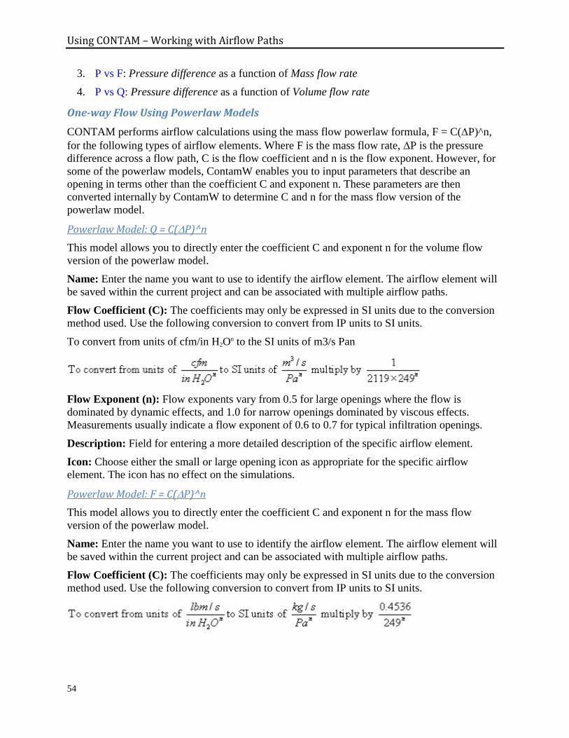
Using CONTAM – Working with Airflow Paths
54
3. P vs F: Pressure difference as a function of Mass flow rate
4. P vs Q: Pressure difference as a function of Volume flow rate
One-way Flow Using Powerlaw Models
CONTAM performs airflow calculations using the mass flow powerlaw formula, F = C(P)^n,
for the following types of airflow elements. Where F is the mass flow rate, P is the pressure
difference across a flow path, C is the flow coefficient and n is the flow exponent. However, for
some of the powerlaw models, ContamW enables you to input parameters that describe an
opening in terms other than the coefficient C and exponent n. These parameters are then
converted internally by ContamW to determine C and n for the mass flow version of the
powerlaw model.
Powerlaw Model: Q = C(P)^n
This model allows you to directly enter the coefficient C and exponent n for the volume flow
version of the powerlaw model.
Name: Enter the name you want to use to identify the airflow element. The airflow element will
be saved within the current project and can be associated with multiple airflow paths.
Flow Coefficient (C): The coefficients may only be expressed in SI units due to the conversion
method used. Use the following conversion to convert from IP units to SI units.
To convert from units of cfm/in H2On to the SI units of m3/s Pan
Flow Exponent (n): Flow exponents vary from 0.5 for large openings where the flow is
dominated by dynamic effects, and 1.0 for narrow openings dominated by viscous effects.
Measurements usually indicate a flow exponent of 0.6 to 0.7 for typical infiltration openings.
Description: Field for entering a more detailed description of the specific airflow element.
Icon: Choose either the small or large opening icon as appropriate for the specific airflow
element. The icon has no effect on the simulations.
Powerlaw Model: F = C(P)^n
This model allows you to directly enter the coefficient C and exponent n for the mass flow
version of the powerlaw model.
Name: Enter the name you want to use to identify the airflow element. The airflow element will
be saved within the current project and can be associated with multiple airflow paths.
Flow Coefficient (C): The coefficients may only be expressed in SI units due to the conversion
method used. Use the following conversion to convert from IP units to SI units.
Using CONTAM – Working with Airflow Paths
55
Flow Exponent (n): Flow exponents vary from 0.5 for large openings where the flow is
dominated by dynamic effects, and 1.0 for narrow openings dominated by viscous effects.
Measurements usually indicate a flow exponent of 0.6 to 0.7 for typical infiltration openings.
Description: Field for entering a more detailed description of the specific airflow element.
Icon: Choose either the small or large opening icon as appropriate for the specific airflow
element. The icon has no effect on the simulations.
Powerlaw Model: Leakage Area
Leakage area refers to a description of airflow features given in Chapter 26 of the 2001
ASHRAE Handbook of Fundamentals [ASHRAE 2001]. Table 1 of this reference provides
typical leakage areas for residential buildings.
Name: Enter the name you want to use to identify the airflow element. The airflow element will
be saved within the current project and can be associated with multiple airflow paths.
Leakage Area: There are three possible ways to enter the leakage area: per item, per unit length,
and per area. Select the radio button for the type of leakage area to be described, then enter the
appropriate value for the type of leakage selected.
Per Item: Enter a total leakage value for an item, this is usually used for a doorway or window -
something that can be classified as an item.
Per Unit Length: Commonly used to describe an interface such as a wall/ceiling junction.
Per Unit Area: Used to describe an area such as a wall or floor.
Reference Conditions: Be sure to check the reference condition for the reported leakage areas.
Two sets of reference conditions are common [ASHRAE 2005 p 27.13]:
Discharge coefficient of 1.00 at a reference pressure difference of 4.0 Pa and
Discharge coefficient of 0.611 at a reference pressure difference of 10 Pa.
Discharge Coefficient: Enter the discharge coefficient for the leakage area at the reference
pressure difference.
Flow Exponent: Enter the flow coefficient for the leakage area at the reference pressure
difference. The flow exponent is not reported and therefore must be estimated. For openings
associated with infiltration, measurements usually indicate an exponent between 0.6 and 0.7.
Pressure Difference: Enter the reference pressure difference for the associated leakage rating.
Description: Field for entering a more detailed description of the specific airflow element.
Icon: Choose either the small or large opening icon as appropriate for the specific airflow
element. The icon has no effect on the simulations.
Powerlaw Model: Connection (ASCOS)
The ASCOS connection element is provided for compatibility with the ASCOS program [Klote
1982]. It is an implementation of the more general orifice flow element based upon the orifice
equation.
Q = K Ao (2 P / )
Using CONTAM – Working with Airflow Paths
56
The inputs for the ASCOS connection are the opening area, Ao, and the dimensionless flow
coefficient, K. Data describing a connection are reduced to the powerlaw model with an
exponent of 0.5. The orifice flow element (see Powerlaw Model: Orifice Area) provides a more
general implementation.
Name: Enter the name you want to use to identify the airflow element. The airflow element will
be saved within the current project and can be associated with multiple airflow paths.
Flow Coefficient: The flow coefficient K is related to the dynamic effects and is typically close
to 0.6 for an orifice and slightly higher for other openings in buildings.
Flow Area: Ao, refers to the observable area of the opening.
Description: Field for entering a more detailed description of the specific airflow element.
Icon: Choose either the small or large opening icon as appropriate for the specific airflow
element. The icon has no effect on the simulations.
Powerlaw Model: Orifice Area
This airflow element allows you to input the description of an orifice.
Name: Enter the name you want to use to identify the airflow element. The airflow element will
be saved within the current project and can be associated with multiple airflow paths.
Cross-sectional Area: This refers to the observable area of the opening.
Flow Exponent (n): Flow exponents vary from 0.5 for large openings where the flow is
dominated by dynamic effects, and 1.0 for narrow openings dominated by viscous effects.
Measurements usually indicate a flow exponent of 0.6 to 0.7 for typical infiltration openings.
Discharge Coefficient: The discharge coefficient, C, is related to the dynamic effects and is
typically close to 0.6 for a sharp-edged orifice and slightly higher for other openings in
buildings.
Hydraulic Diameter: The hydraulic diameter is equal to (4 Area / Perimeter). For square
openings this equals the square root of the area, and for long thin openings it is two times the
width.
Reynolds Number: The transition from laminar flow to turbulent flow occurs over a very broad
range of Reynolds numbers with the flow being fully laminar approximately below 100.
Note: The hydraulic diameter and Reynolds number have little impact on the calculations.
Generally you should use the default values except for special circumstances where you need
them to be modified. The parameters above describe the flow characteristics of an orifice in
typical operation. At extremely low pressure drops the use of the powerlaw model leads to a
division by zero during the network solution process. ContamX avoids this problem by changing
to a linear model in this region. The model is based conceptually on the flow changing from
turbulent to laminar at very low pressures. The Hydraulic diameter and Reynolds number are
used to determine a point where the model changes from the powerlaw to linear.
Description: Field for entering a more detailed description of the specific airflow element.
Icon: Choose either the small or large opening icon as appropriate for the specific airflow
element. The icon has no effect on the simulations.
Using CONTAM – Working with Airflow Paths
57
Powerlaw Model: Crack Description
This airflow element allows you to enter the description of a crack and is based upon the
relationships developed between flow through cracks and the powerlaw model [Clark 1985].
Name: Enter the name you want to use to identify the airflow element. The airflow element will
be saved within the current project and can be associated with multiple airflow paths.
Crack Length/Width: Enter the length and width of the crack.
Description: Field for entering a more detailed description of the specific airflow element.
Note: ContamW automatically uses the icon for a small opening for the powerlaw model crack
description.
Powerlaw Model: Test Data (1 point)
This airflow element allows you to provide a single test data point that ContamW reduces to the
powerlaw model by calculating the flow coefficient based on input values (See Fitting Powerlaw
Coefficients in the Theoretical Background section).
Name: Enter the name you want to use to identify the airflow element. The airflow element will
be saved within the current project and can be associated with multiple airflow paths.
Pressure Difference (P): Enter the pressure difference for the data point.
Flow Rate (F): Enter the flow rate for the data point.
Pressure Exponent (n): The flow exponent is a guess used to fit the single point to the
powerlaw model. A value of 0.6 to 0.7 is typical for an infiltration element. A value of 0.5 is
more appropriate for large openings.
Description: Field for entering a more detailed description of the specific airflow element.
Icon: Choose either the small or large opening icon as appropriate for the specific airflow
element. The icon has no effect on the simulations.
Powerlaw Model: Test Data (2 points)
This airflow element allows you to provide two test data points that ContamW reduces to the
powerlaw model by calculating the flow coefficient based on input values (See Fitting Powerlaw
Coefficients in the Theoretical Background section).
Name: Enter the name you want to use to identify the airflow element. The airflow element will
be saved within the current project and can be associated with multiple airflow paths.
Pressure Difference (P): Enter the pressure difference for each of the two data points.
Flow Rate (F): Enter the flow rate for each data point.
Description: Field for entering a more detailed description of the specific airflow element.
Icon: Choose either the small or large opening icon as appropriate for the specific airflow
element. The icon has no effect on the simulations.
Powerlaw Model: Stairwell
This airflow element allows you to enter a description of a stairway, which ContamW converts to
a powerlaw relationship assuming a pressure exponent of 0.5. A stairwell will normally be
Using CONTAM – Working with Airflow Paths
58
modeled as a vertical series of zones connected by low resistance openings (this stairwell flow
element) through the floors. The resistance is based on a fit to experimental data [Achakji &
Tamura 1998]. This model should only be used between zones on different levels of a building
(paths through floors), not between zones on the same level (paths through walls).
Name: Enter the name you want to use to identify the airflow element. The airflow element will
be saved within the current project and can be associated with multiple airflow paths.
Distance Between Levels: The vertical distance between doorways of the stairwell. This is
typically equal to the "Distance to level above" of the level below the path with which this
element is to be associated.
Cross-sectional area: This is the horizontal, cross-sectional, area of the shaft.
Density of People: A large number of people in the stairwell influences the flow resistance of
the stairwell. The experiment used densities of 1, 2, and 3 people per square meter. These are the
only units available in ContamW. The following conversion is provided for your convenience.
1 m2 = 10.76 ft2
Stair Treads: There are two options for this field: open tread and closed tread. This refers to the
front of the tread whether or not the tread is open effects flow.
Description: Field for entering a more detailed description of the specific airflow element.
Icon: Choose either the small or large opening icon as appropriate for the specific airflow
element. The icon has no effect on the simulations.
Powerlaw Model: Shaft
This airflow element allows you to enter a description of a shaft, and ContamW converts the
information to a powerlaw relationship assuming a pressure exponent of 0.5. A shaft will
normally be modeled as a vertical series of zones connected by low resistance openings (this
shaft airflow element) through the floors. The resistance is based on a conduit friction model
using the Darcy-Weisbach relation and Colebrook’s equation for the friction factor [ASHRAE
2005, p2.7].
Name: Enter the name you want to use to identify the airflow element. The airflow element will
be saved within the current project and can be associated with multiple airflow paths.
Distance Between Levels: This is the distance between openings for the stairwell.
Cross-sectional area: This is the horizontal, cross-sectional, area of the shaft, not the opening.
Perimeter: The perimeter of the horizontal cross-section of the shaft. This number is used in
conjunction with the area to create the hydraulic diameter.
Roughness: This refers to the average size of the protrusions from the shaft wall into the airflow.
Description: Field for entering a more detailed description of the specific airflow element.
Icon: Choose either the small or large opening icon as appropriate for the specific airflow
element. The icon has no effect on the simulations.
Using CONTAM – Working with Airflow Paths
59
One-way Flow Using Quadratic Flow Models
ContamX performs airflow calculations using the mass flow quadratic relationship
(P = aF + bF²) between mass flow rate and pressure difference across a flow path for the
following types of airflow elements. Where F is the mass flow rate, P is the pressure difference
across a flow path, and a and b are flow coefficients.
Quadratic Model: P = aQ + bQ²
This model allows you to directly enter the coefficients, a and b, into the volume flow version of
the quadratic flow model. Where P is the pressure drop and Q is the volumetric flow rate.
Name: Enter the name you want to use to identify the airflow element. The airflow element will
be saved within the current project and can be associated with multiple airflow paths.
Coefficients: The coefficients must be expressed in SI units because of the way ContamW
handles unit conversions. The units of the coefficients at standard conditions, i.e., sm3/s, are as
follows:
a [Pa • s/sm3]
b [Pa • (s/sm3)2]
To convert from volume flow Q in units of m3/s at density to sm
3/s at density s, multiply Q
by /s, where s equals 1.2041 kg/m3 at 20 °C.
Description: Field for entering a more detailed description of the specific airflow element.
Icon: Choose either the small or large opening icon as appropriate for the specific airflow
element. The icon has no effect on the simulations.
Quadratic Model: P = aF + bF²
This model allows you to directly enter the coefficients, a and b, into the mass flow version of
the quadratic flow model. Where P is the pressure drop and F is the mass flow rate.
Name: Enter the name you want to use to identify the airflow element. The airflow element will
be saved within the current project and can be associated with multiple airflow paths.
Coefficients: The coefficients must be expressed in SI units because of the way ContamW
handles unit conversions. The units of the coefficients are as follows:
Description: Field for entering a more detailed description of the specific airflow element.
Icon: Choose either the small or large opening icon as appropriate for the specific airflow
element. The icon has no effect on the simulations.
Quadratic Model: Crack Description
This model employs a quadratic relationship of the form P = aQ + bQ² where Q is the volume
flow rate [Baker, Sharples, and Ward 1987]. CONTAM uses the mass flow version of that
formula: P = aF + bF² where P is the pressure drop and F is the mass flow rate.

Using CONTAM – Working with Airflow Paths
60
Name: Enter the name you want to use to identify the airflow element. The airflow element will
be saved within the current project and can be associated with multiple airflow paths.
Crack Dimensions:
Length: The overall length of the crack
Width: Width of the crack
Depth: The distance along the direction of airflow
Number of Bends: The number of bends in the flow path.
Description: Field for entering a more detailed description of the specific airflow element.
Quadratic Model: Test Data (2 points)
Measured data (2 points) is reduced to the mass flow version of the quadratic model.
Name: Enter the name you want to use to identify the airflow element. The airflow element will
be saved within the current project and can be associated with multiple airflow paths.
Data: Data consists of two sets of pressure drops and corresponding flow rates.
Description: Field for entering a more detailed description of the specific airflow element.
Icon: Choose either the small or large opening icon as appropriate for the specific airflow
element. The icon has no effect on the simulations.
Two-way Flow Models
These models enable you to simulate openings through which two-way airflow might occur (e.g.
doorways and open windows). When viewing results of these models, the bidirectional flow will
be indicated on the SketchPad if it occurs. You can also use ContamW’s airflow plotting feature
to plot both airflows or to simply plot the net airflow. There must be a density difference across
the associated airflow path in order for bidirectional flow to occur across these types of airflow
elements. See Doorways (Large Openings) in the Theory section for a more detailed explanation.
The Relative Elevation of flow paths that implement these models should be set to the bottom of
the flow path as opposed to the mid-height used for other element types.
Two-way Flow Model: Single Opening
This is a model for flow through large openings such as doorways through which air can flow in
two directions simultaneously throughout the opening.
Name: Enter the name you want to use to identify the airflow element. The airflow element will
be saved within the current project and can be associated with multiple airflow paths.
Height: The overall height of the opening, not to be confused with the Relative Elevation of flow
paths with which the element is associated.
Width: The width of the opening. Again, before entering the dimension make sure to select the
proper units from the drop down menu.
Flow Coefficient: An experimentally determined value. Experiments by Weber and Kearney
[Weber and Kearney 1989] have shown the default value of 0.78 to work well for most
applications.
Using CONTAM – Working with Airflow Paths
61
Minimum Temperature Difference for Two-Way Flow: A two-way flow is driven by the
temperature (actually air density) difference between the two zones. When this temperature
difference approaches zero the algorithm used for solving the flow tends towards a division by
zero problem. To avoid this undefined situation the two-way model reverts to a one-way power
law model at this "minimum temperature difference" using the opening size to define the orifice
at T set in this field. ContamW uses a default value of 0.01 C.
Description: Field for entering a more detailed description of the specific airflow element.
Icon: Choose either the small or large opening icon as appropriate for the specific airflow
element. The icon has no effect on the simulations.
Two-way Flow Model: Two-opening
This model accounts for two-way flow due to the stack effect acting over the height of a tall
opening. It uses two power law flow models at different heights to approximate a single tall
opening.
Name: Enter the name you want to use to identify the airflow element. The airflow element will
be saved within the current project and can be associated with multiple airflow paths.
Height: The overall height of the opening, not to be confused with the Relative Elevation of flow
paths with which the element is associated.
Width: The width of the opening.
Flow Coefficient: This is an experimentally determined value. Experiments by Weber and
Kearney have shown the default value of 0.78 to work well for most applications.
Description: Field for entering a more detailed description of the specific airflow element.
Icon: Choose either the small or large opening icon as appropriate for the specific airflow
element. The icon has no effect on the simulations.
Backdraft Damper Models
The Backdraft Damper models make it possible to model a feature that has different flow
resistances depending on the direction of the pressure drop, with greatly reduced (or zero) flow
in one direction. Note that there are similar models available for duct flow elements.
Backdraft Damper Model: Q = C(P)^n
This is the volumetric flow form of the backdraft damper airflow model.
Name: Enter the name you want to use to identify the airflow element. The airflow element will
be saved within the current project and can be associated with multiple airflow paths.
Pressure Difference: Enter a flow coefficient and exponent for both the positive and negative
flow directions of the flow path. P>0 refers to the pressure difference across the flow element
that would lead to an airflow in the positive flow direction (See Airflow Path Properties) and
P<0 would lead to a flow in the opposite direction.
Flow Coefficients: The coefficients may only be expressed in SI units due to the conversion
method used. Use the following conversion to convert from IP units to SI units.
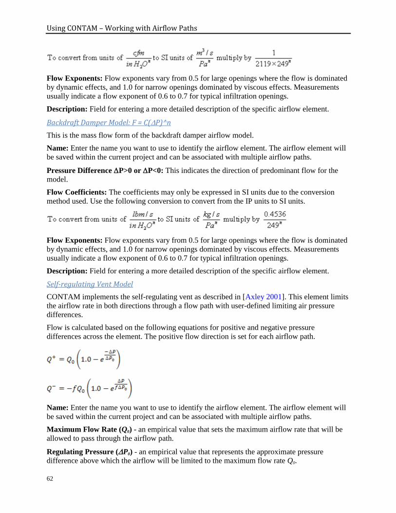
Using CONTAM – Working with Airflow Paths
62
Flow Exponents: Flow exponents vary from 0.5 for large openings where the flow is dominated
by dynamic effects, and 1.0 for narrow openings dominated by viscous effects. Measurements
usually indicate a flow exponent of 0.6 to 0.7 for typical infiltration openings.
Description: Field for entering a more detailed description of the specific airflow element.
Backdraft Damper Model: F = C(P)^n
This is the mass flow form of the backdraft damper airflow model.
Name: Enter the name you want to use to identify the airflow element. The airflow element will
be saved within the current project and can be associated with multiple airflow paths.
Pressure Difference P>0 or P<0: This indicates the direction of predominant flow for the
model.
Flow Coefficients: The coefficients may only be expressed in SI units due to the conversion
method used. Use the following conversion to convert from the IP units to SI units.
Flow Exponents: Flow exponents vary from 0.5 for large openings where the flow is dominated
by dynamic effects, and 1.0 for narrow openings dominated by viscous effects. Measurements
usually indicate a flow exponent of 0.6 to 0.7 for typical infiltration openings.
Description: Field for entering a more detailed description of the specific airflow element.
Self-regulating Vent Model
CONTAM implements the self-regulating vent as described in [Axley 2001]. This element limits
the airflow rate in both directions through a flow path with user-defined limiting air pressure
differences.
Flow is calculated based on the following equations for positive and negative pressure
differences across the element. The positive flow direction is set for each airflow path.
Name: Enter the name you want to use to identify the airflow element. The airflow element will
be saved within the current project and can be associated with multiple airflow paths.
Maximum Flow Rate (Q0) - an empirical value that sets the maximum airflow rate that will be
allowed to pass through the airflow path.
Regulating Pressure (P0) - an empirical value that represents the approximate pressure
difference above which the airflow will be limited to the maximum flow rate Q0.
Using CONTAM – Working with Airflow Paths
63
Reverse Flow Fraction (f) - the fraction of the Maximum Flow Rate to which the airflow
through this element will be limited when the pressure difference is negative across the airflow
path.
Description - You can provide a more detailed note to describe this airflow element.
Fan and Forced Flow Models
These airflow element models enable you to easily create forced airflow elements as airflow
paths between two zones, as opposed to implementing a duct model or simple air handling
system. There are three types of fan models to choose from: constant mass flow rate, constant
volumetric flow rate, and fan performance curve.
Fan Model: Constant Mass Flow Fan
This model describes an airflow element having a constant mass flow rate. This airflow element
will provide the specified constant mass flow rate regardless of the density of the air being
delivered by the fan.
Name: Enter the name you want to use to identify the airflow element. The airflow element will
be saved within the current project and can be associated with multiple airflow paths.
Design (maximum) Flow: Enter the maximum mass flow rate. This value can be modified by
the path schedule.
Description: Field for entering a more detailed description of the specific airflow element.
Fan Model: Constant Volume Flow Fan
This model describes an airflow element having a constant volume flow rate. The design flow
rate you specify is in terms of standard air. CONTAM uses a density of 1.204 kg/m3 based on
conditions specified by ASHRAE for dry air: 101.325 kPa and 20 ºC (ASHRAE 2004, p 18.4).
Therefore, if actual conditions during simulation do not match these standard conditions, the
results will differ from specified flow due to differences in air density.
Name: Enter the name you want to use to identify the airflow element. The airflow element will
be saved within the current project and can be associated with multiple airflow paths.
Design (maximum) Flow: Enter the maximum volume flow rate. This value can be modified by
the path schedule.
Description: Field for entering a more detailed description of the specific airflow element.
Fan Model: Fan Performance Curve
This airflow element allows you to create a fan based on a fan performance curve. You provide
ContamW with a set of pressure rise and airflow rate data points, and ContamW performs a
polynomial curve fit to the data. Airflow rates are specified in mass flow units for standard air.
Name: Enter the name you want to use to identify the airflow element. The airflow element will
be saved within the current project and can be associated with multiple airflow paths.
Fan off conditions: These values specify how the fan is modeled when the speed of the fan is
insufficient to provide a flow.
Cut-off Ratio: The fan speed ratio is the actual speed (RPM) of the fan divided by the rated
speed of the fan (fan is defined for a speed ratio of 1.0). When this ratio is below the
Using CONTAM – Working with Airflow Paths
64
specified cut-off limit the fan is modeled as a simple orifice based on the "equivalent orifice"
defined for this fan element. During a simulation, ContamX obtains the actual ratio from the
control value being applied (in the form of a schedule or control signal) to the airflow path
with which this fan element is associated and compares it to the cut-off ratio. See Chapter 18
Fans in [ASHRAE 2004].
Equivalent Orifice: The size of the orifice used to model the fan opening when the control
value drops below the specified limit.
Description: Field for entering a more detailed description of the specific airflow element.
Fan Performance Data: Click the "Edit Fan Curve Data" to input/modify the fan curve for this
airflow element. A detailed explanation of this data is given in the next section, Fan Performance
Data.
Fan Performance Data
Between four and ten data points are required for ContamW to fit a cubic polynomial to create a
performance curve for the fan. The fitted curve may not contain a point of contraflecture; if it
does an error message will be displayed. If this error message is displayed the pressure rise data
must then be modified to eliminate the point of contraflecture.
Entering Fan Curve Data Points You only need to fill in the "Flow rate" and "Pressure rise" data entry when entering fan curve
data. When adding a new data point, the flow rate must be entered in the "Flow rate" edit box
and the pressure rise must be entered in the "Pressure rise" edit box. Use the "Revised dP" box
when making changes to a pressure rise that has already been entered. This will preserve the
original data point but use the revised value when performing the curve fit. After entering the
flow rate and the pressure rise into the appropriate edit boxes, the next step is to press the "<<
Insert <<" button. Once you have entered four data points a cubic fit will automatically be
generated and displayed as a line on the graph.
Revising Fan Curve Data Points To edit existing data points, highlight the line of data to revise in the list of Fan Curve Data to
the left of the Insert, Replace and Delete buttons. The values from that data set will then appear
in the edit boxes to the right of the buttons.
If you need to modify the flow rate, enter the new flow rate in the "Flow rate" edit box and then
press the "<< Replace <<" button. The new data will now replace the old data.
If the Pressure Rise needs to be modified there are two available options:
1. Replace the data point completely. To overwrite an existing pressure rise and refit the fan
curve, select the data set to be modified by highlighting it in the data list and then type the
new pressure rise in the "Pressure rise" edit box then press the "<< Replace <<" button.
2. Change the point used to fit the cubic polynomial but leave the marker for the original data
point intact. With this option you may "tweak" the curve in the event there is some issue
with the originally entered fan curve, such as a point of contraflecture.
Using CONTAM – Working with Airflow Paths
65
Cubic Spline Models
Cubic spline models enable you to create airflow elements based on a curve fit to a user-defined
set of data points. The cubic spline fit used to generate the curve guarantees a first-order
differentiable relationship between flow and pressure as required by the CONTAM solver.
During simulation, the sign of the pressure difference will be based on the Positive Flow
Direction defined for the flow paths with which the spline elements are associated. For example,
a drop in pressure in the direction of positive flow (i.e. Pressure in from zone – Pressure in to
zone > 0) will utilize a positive pressure from the spline data.
There are some basic requirements for each of these elements. They require a minimum of four
data points, so a curve will not be displayed until the minimum number of points is entered. All
models require that the slope be greater than zero for all segments of the curve fit. If there is an
error in the curve fit when you click the OK button, an error message will be displayed indicating
the offending segments of the curve and a reason for the error. Segments are numbered from zero
to the number of data points minus one. For example – "seg 0: y’ <= 0" will be displayed if
the segment between the first two data points has a slope less than or equal to zero.
Name: Enter the name you want to use to identify the airflow element.
Description: Field for entering a more detailed description of the specific airflow element.
Curve Data: Create and edit the list of data points to define the curve for the airflow element.
The type of cubic spline element you are editing determines the independent and dependent
variables for the curve. The labels of the list, data entry fields and associated units will change
accordingly, as will the axes of the plot. Use the data entry fields along with the "Add" button to
create new and edit existing data points. Use the "Delete" button to remove the currently selected
data point from the list.
Icon: Choose either the small or large opening icon as appropriate for the specific airflow
element. The icon has no effect on the simulations.
Cubic Spline: F vs P
Mass flow as a function of Pressure drop across the element.
Cubic Spline: Q vs P
Volume flow as a function of Pressure drop across the element.
Cubic Spline: P vs F
Pressure drop as a function of Mass flow through the element.
Cubic Spline: P vs Q
Pressure drop as a function of Volume flow through the element.

Using CONTAM – Working with Simple Air-handling Systems
66
3.6 WORKING WITH SIMPLE AIR-HANDLING SYSTEMS
The simple air-handling system (AHS) provides a convenient means of incorporating an air-
handling system into a building without having to draw and define an entire duct system. Each
simple air-handling system consists of two implicit airflow nodes or zones (supply and return
sub-systems), three implicit flow paths (recirculation, outdoor, and exhaust), and multiple zone
supplies (inlets to zones) and zone returns (outlets from zones) that you can place within zones
throughout the building. You specify the airflow rates of each supply and return point. Simple
air-handling systems do not require you to associate both zone supplies and zone returns with
them. You may use the simple air-handling system to only supply outdoor (ambient) air to a
building or to only exhaust air from the building. The following figure shows a schematic
representation of a simple air-handling system.
Determination of System Airflows ContamX determines the airflows rates associated with each air-handling system according to the
following algorithm. More detailed explanations for the values that you must input for this
algorithm are explained in the Defining Air-handling Systems section that follows.
First, all of the user-defined supply (supply air to the zones) and return (return air from the
zones) airflow (mass) rates are summed.
Ws the sum of all supplies
Wret the sum of all returns
The amount of outdoor air that the system requires is then determined by
W'o = max( fo·Ws, min(Ws, Wo_min ) ),
where, fo the fraction outdoor air = Wo/Ws
Using CONTAM – Working with Simple Air-handling Systems
67
You input this parameter as the Outside Air Schedule of a simple air handling system (See Air
Handling System – AHS Properties), and
Wo_min the "minimum outdoor airflow" parameter that you input.
The rate at which air is recirculated via the implicit recirculation flow path, Wrec, is determined
by
Wrec = min(Wret, Ws - W'o ).
The rate at which outdoor air is brought in by the system via the implicit outdoor airflow path,
Wo, is determined by
Wo = Ws - Wrec.
And the rate at which exhaust airflows to the ambient via the implicit exhaust flow path, Wex, is
determined by
Wex = Wret - Wrec.
Based on this algorithm the amount of outdoor air the system will provide, Wo, will be between
Wo_min and fo·Ws as long as the demand for supply air, Ws, is sufficient to provide this value.
Otherwise the system will provide Ws. When the sum of the supply flows, Ws, exceeds the
sum of the return flows, Wret, the balance is made up of outdoor air. Any excess return air is
exhausted via the implicit exhaust flow path.
3.6.1 Creating Simple Air-handling Systems
You create simple air-handling systems by placing an Air-handling System (AHS) icon on the
SketchPad along with some combination of supply and/or return icons (See Drawing Building
Component Icons). You may place an AHS icon on any blank cell of the SketchPad on any level.
You do not have to place it within a zone. However, you must place Supply icons and Return
icons within a zone. The pop-up menu selections will be disabled (grayed out) if you pop-up on a
location where ContamW does not allow these icons to be placed.
3.6.2 Deleting Air-handling Systems
You delete icons related to simple air-handling systems using the icon deletion procedure (See
Deleting Building Component Icons). If you delete an AHS icon, , all of the supplies and
returns associated with that system will be deleted. You will be warned of this when you attempt
to delete the icon. However, you can delete individual supplies and returns without affecting any
other icons. Deleting any AHS-related icons from the SketchPad does not delete any filter,
schedule, or kinetic reaction elements that you may have defined for the AHS. These flow
elements can only be deleted using the CONTAM Library Manager, accessible through the Data
menu for each type of data element.
3.6.3 Modifying Air-handling Systems
To modify the parameters of a simple air-handling system, you use the icon definition procedure
(See Defining Building Component Icons) to display its properties and make the desired
changes. You can move air-handling system icons and move and copy supply and return icons;
however, you cannot copy air-handling system icons.
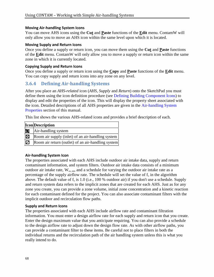
Using CONTAM – Working with Simple Air-handling Systems
68
Moving Air-handling System Icons You can move AHS icons using the Cut and Paste functions of the Edit menu. ContamW will
only allow you to move an AHS icon within the same level upon which it is located.
Moving Supply and Return Icons Once you define a supply or return icon, you can move them using the Cut and Paste functions
of the Edit menu. ContamW will only allow you to move a supply or return icon within the same
zone in which it is currently located.
Copying Supply and Return Icons Once you define a supply or return icon using the Copy and Paste functions of the Edit menu.
You can copy supply and return icons into any zone on any level.
3.6.4 Defining Air-handling Systems
After you place an AHS-related icon (AHS, Supply and Return) onto the SketchPad you must
define them using the icon definition procedure (see Defining Building Component Icons) to
display and edit the properties of the icon. This will display the property sheet associated with
the icon. Detailed descriptions of all AHS properties are given in the Air-handling System
Properties section of this manual.
This list shows the various AHS-related icons and provides a brief description of each.
Icon Description
Air-handling system
Room air supply (inlet) of an air-handling system
Room air return (outlet) of an air-handling system
Air-handling System Icon The properties associated with each AHS include outdoor air intake data, supply and return
contaminant information, and system filters. Outdoor air intake data consists of a minimum
outdoor air intake rate, Woa_min and a schedule for varying the outdoor air intake rate as a
percentage of the supply airflow rate. The schedule will set the value of fo in the algorithm
above. The default value of fo is 1.0 (i.e., 100 % outdoor air) if you don't use a schedule. Supply
and return system data refers to the implicit zones that are created for each AHS. Just as for any
zone you create, you can provide a zone volume, initial zone concentration and a kinetic reaction
for each contaminant defined for the project. You can also associate contaminant filters with the
implicit outdoor and recirculation flow paths.
Supply and Return Icons The properties associated with each AHS include airflow rate and contaminant filtration
information. You must enter a design airflow rate for each supply and return icon that you create.
Enter the design maximum value that you anticipate requiring. You can also provide a schedule
to the design airflow rate to adjust down the design flow rate. As with other airflow paths, you
can provide a contaminant filter to these items. Be careful not to place filters in both the
individual returns and the recirculation path of the air handling system unless this is what you
really intend to do.
Using CONTAM – Working with Simple Air-handling Systems
69
3.6.5 Air-handling System Properties
This section provides detailed descriptions of the specific properties of simple air-handling
systems. Each of the following subsections are the context-sensitive help topics that you can
access by pressing F1 when working with property pages of the "Simple Air-handling System
Properties," "Supply Point Properties," and "Return Point Properties" property sheets.
Air-handling System - AHS Properties
System Name: The name used to identify the Air-handling System. Air-handling system names
must be unique.
Minimum OA Flow: This is the minimum outdoor air introduced into the AHS supply flow. If
the sum of the return flows plus the minimum outside airflow exceeds the total supply flow then
the excess return air is exhausted. Similarly if the return flow plus the minimum outdoor airflow
do not sum to the supply flow then outdoor air is brought in to make up the difference.
Outdoor Air Schedule: This is a schedule of the fraction of outdoor air, fo, to be introduced to
the simple air handling system. If the schedule is set to "<none>", then the fraction of outdoor air
defaults to 100 % (100 %outdoor air, 100 % exhaust and no recirculation). You define a new
Outdoor Air schedule by pressing the "New Schedule" button and following the procedure for
editing a Week Schedule.
Name: This drop down box contains the names of all previously defined schedules within the
current project. You can select an existing schedule from the list and use the "Edit Schedule"
button to view and modify its properties, create a "New Schedule" and even select a schedule
from a CONTAM Library via the "Library..." button. You can also choose to not apply a
schedule by selecting "<none>" from the list.
Description: Displays the detailed description of the selected outdoor air schedule.
CVF/DVF Control: Values from either a CVF or DVF file can be used in place of the above
Schedule (read about CVF and DVF controls in the Control Element Types section). This
enables using these control element types without having to draw/define an associated control
network. The associated radio buttons "Use Neither", "Use CVF" and "Use DVF" are used to
select the desired control method. Select the heading name from the associated "Name" drop
down box that will display the headings of either the CVF or DVF file as per the aforementioned
radio button selection.
Control Status: This will display the current method of control: Schedule, direct CVF, direct
DVF or Control Network. If an actuator of a control network on the SketchPad is associated with
the scheduled item then it will take precedence over the Schedule and CVF/DVF Control. If
either the "Use CVF" or "Use DVF" radio button is selected then CVF or DVF will take
precedence over an associated schedule.
Outdoor Air Intake Location: These are the absolute X, Y and Z coordinates and units that
define the location of the outdoor air intake of the selected air handling system. These values are
required when using a Wind Pressure and Contaminant (WPC) file (see Working with WPC
Files).
Using CONTAM – Working with Simple Air-handling Systems
70
NOTE: You must first check either the Wind Pressures or Contaminant Concentrations check
boxes on the Wind Pressure and Contaminants (WPC) File Parameters dialog box to be able to
access these coordinate input fields (see Create WPC File Dialog).
Air-handling System - Supply System Properties
System Volume: Enter a value for the supply sub-system (implicit supply zone) of the simple air
handler (e.g., supply-side duct work etc.). This volume is very similar to a zone volume and will
be used in the simulation of contaminant transport.
Contaminant Data: All of the defined contaminants in the project will be displayed in this list
box.
Initial Concentration: Select a contaminant from the list and enter the initial contaminant
concentrations for the supply air sub-system of this simple air handling system. Note that only
those species you have selected to be contaminants (to use during simulation) appear in the list.
If a species for which you wish to set an initial concentration does not appear in the list you must
set the "Use in simulation" property of the corresponding species to be true (See Creating
Species and Contaminants). You can reset these initial values through the Run Control Properties
of the Simulation Parameters.
NOTE: Changing the number of contaminants, i.e. those species used in the simulation, will
reset the initial concentrations of all zones to the default contaminant concentrations. You can
reset all of these concentrations via the Run Control Properties as indicated above or individually
here.
Sum of Non-trace Initial Concentrations: This value is provided as a check for you to insure
that you input a reasonable set of initial values when using non-trace contaminants. This value
should be very close to 1.0.
Kinetic Reaction: You define a new kinetic reaction by pressing the "New Reaction" button and
then completing the kinetic reaction matrix. You can edit an existing matrix by selecting the
proper matrix from the drop down box and pressing the "Edit Reaction" button. You must have
previously defined contaminants in order to implement a kinetic reaction.
Description: Field that shows a more detailed description of the specific reaction if entered
by the user. This description can be modified by pressing the "Edit Reaction" button next to
the description field and then changing the description field for the reaction.
Name: This contains a list of names of all previously created reactions. The reaction selected
from this box will define the behavior of the specific supply system being modified.
Air-handling System - Return System Properties
System Volume: Enter a value for the return sub-system (implicit return zone) of the simple air
handler (e.g., return-side duct work etc.). This volume is very similar to a zone volume and will
be used in the simulation of contaminant transport.
Contaminant Data: All of the defined contaminants in the project will be displayed in this list
box.
Initial Concentration: Select a contaminant from the list and enter the initial contaminant
concentrations for the return air sub-system of this simple air handling system. Note that only
those species you have selected to be contaminants (to use during simulation) appear in the list.
Using CONTAM – Working with Simple Air-handling Systems
71
If a species for which you wish to set an initial concentration does not appear in the list you must
set the "Use in simulation" property of the corresponding species to be true (see Creating Species
and Contaminants). You can reset these initial values through the Run Control Properties of the
Simulation Parameters.
NOTE: Changing the number of contaminants, i.e. those species used in the simulation, will
reset the initial concentrations of all zones to the default contaminant concentrations. You can
reset all of these concentrations via the Run Control Properties as indicated above or individually
here.
Sum of Non-trace Initial Concentrations: This value is provided as a check for you to insure
that you input a reasonable set of initial values when using non-trace contaminants. This value
should be very close to 1.0.
Kinetic Reaction: You define a new kinetic reaction by pressing the "New Reaction" button and
then completing the kinetic reaction matrix. You can edit an existing matrix by selecting the
proper matrix from the drop down box and pressing the "Edit Reaction" button. You must have
previously defined contaminants in order to implement a kinetic reaction.
Description: Field that shows a more detailed description of the specific reaction if entered
by the user. This description can be modified by pressing the "Edit Reaction" button next to
the description field and then changing the description field for the reaction.
Name: This contains a list of names of all previously created reactions. The reaction selected
from this box will define the behavior of the specific return system being modified.
Air-handling System - Filter Properties
As the names suggest, outdoor air filters affect the air brought in by the simple air-handling
system from outside the building, while recirculation air filters affect the return air being
circulated back through the air handler. You may either create, edit or delete the filters associated
with the implicit outdoor air and recirculation flow paths of the simple air-handler. Creating a
new filter or modifying an existing one will display the Filter dialog box. For an explanation of
contaminant filters see Working with Filters in the Using CONTAM section of the manual.
Supply and Return Point - System Properties
Design Flow Rate: Enter the design maximum airflow rate for the supply or return.
AHS: You must associate each supply and return point with an existing simple air-handling
system.
Name: This drop down box contains the names of all previously created Air-handling
Systems. The AHS selected from this box will define the behavior of the specific
supply/return system being modified. Once an existing AHS is selected it may be edited by
pressing the "Edit AHS" button.
Description: Displays the description of the currently selected Simple AHS.
Location: These are the X, Y and RelHeight (Z) coordinates and units for the selected
supply/return point. X and Y are absolute coordinates and RelHeight is relative to the level on
which the supply/return point is located.
Using CONTAM – Working with Simple Air-handling Systems
72
These values are required for any supply/return point that is located within a 1D
convection/diffusion zone (see 1D Zone Data). These coordinates will be verified by ContamW
against the axis of the 1D zone in which it is located. This verification will be performed
automatically when you select either the Run Simulation or Create a ContamX Input File
command from the Simulation menu.
Supply and Return Point - Schedule Properties
Schedule: You can associate a schedule with the supply/return point to control the fraction of the
design airflow rate that flows to/from the zone in which the supply/return point is located
according to the time of day and day of the week.
Description: Field that shows a more detailed description of the specific schedule if entered
by the user. You can modify this description by pressing the "Edit Schedule" button next to
the description field and then changing the description field for the schedule.
Name: This drop down box contains the names of all previously created schedules. The
schedule selected from this box will define the behavior of the specific supply/return system
being modified.
CVF/DVF Control: Values from either a CVF or DVF file can be used in place of the above
Schedule (read about CVF and DVF controls in the Control Element Types section). This
enables using these control element types without having to draw/define an associated control
network. The associated radio buttons "Use Neither", "Use CVF" and "Use DVF" are used to
select the desired control method. Select the heading name from the associated "Name" drop
down box that will display the headings of either the CVF or DVF file as per the aforementioned
radio button selection.
Control Status: This will display the current method of control: Schedule, direct CVF, direct
DVF or Control Network. If an actuator of a control network on the SketchPad is associated with
the scheduled item then it will take precedence over the Schedule and CVF/DVF Control. If
either the "Use CVF" or "Use DVF" radio button is selected then CVF or DVF will take
precedence over an associated schedule.
Supply and Return Point - Filter Properties
Filter: You may select a previously defined filter from those contained in the associated Name
list. Click the "New Filter" button to define a new filter. Click the "Edit Filter" button to view or
modify existing filter data. Setting this field to <none> indicates no filter for this airflow path.
(See Contaminant Filters under Working with Contaminants)
Using CONTAM – Working with Ducts
73
3.7 WORKING WITH DUCTS
As an alternative to the simple air-handling system, CONTAM allows you to model HVAC
systems using detailed duct systems. Duct systems are made up of duct segments, junctions,
terminal points, and forced air components. A duct segment is a section of a duct between any
two junctions, terminal points or combination of the two. A terminal point is an endpoint of a
duct segment, and a junction is the connection between two to four duct segments. Only
horizontal segments can be displayed on the ContamW SketchPad, but vertical segments can be
implemented as well. Vertical segments are connected with special junctions and terminal points
that reveal the location of the vertical segments on the SketchPad.
You draw the layout of the duct system, and ContamW will insert junctions and terminal points
where appropriate. Once you have drawn a duct system, you must define the drawing by
providing detailed segment, junction and terminal point information. You must provide each duct
segment with specific information that describes the flow characteristics and physical
dimensions of that segment. Much of this information is in the form of duct flow elements that
you create when defining the duct segments. Definition of duct segments, junctions and
terminals can be simplified using the copy and paste commands. The details of drawing and
defining a duct system are described in the following sections.
3.7.1 Duct Flow Elements
Each duct segment must refer to a duct flow element. Duct flow elements describe the
mathematical relationship between flow through and pressure drop along the duct, the flow
resistance or forced flow characteristics, cross-sectional geometry, and optional leakage per unit
length of a duct. ContamW provides you with several different mathematical models or element
types to choose from. Each of these duct flow element types is described in detail in the Duct
Segment Properties section. While every duct segment must refer to a single duct flow element,
multiple duct segments can refer to the same duct flow element. Duct flow elements can also be
stored within a CONTAM library file and shared between different CONTAM project files.
3.7.2 Drawing Ducts
You draw ducts using the duct drawing tool previously described in the Working with the
SketchPad section. After you complete the "finalize drawing object" stage of duct drawing, the
completed duct will appear as an undefined set of red duct icons. The color red indicates that the
duct is not yet defined. Once you have defined the duct components, they will be displayed in
blue. A directional duct segment icon will be displayed within each duct segment, and each
junction and terminal point will be replaced with an icon indicating the type of junction or
terminal point you have defined.
Drawing Duct Segments ContamW provides certain constraints when drawing ducts to insure that a valid duct system will
be drawn that conforms to the underlying model of nodal equations upon which CONTAM is
based. When drawing a duct, you cannot cross over a line that you are currently drawing. Ducts
can cross over walls, but you cannot draw ducts over any other building component icons. After
each duct segment is drawn, the ends of the segment will be automatically replaced by either an
undefined terminal point or junction icon. You can only begin or end a duct segment drawing in
an unoccupied SketchPad cell or on an undefined duct icon. For this reason, you are advised to
draw the entire duct system, on a given level, before you define the individual duct segments. If
Using CONTAM – Working with Ducts
74
you cross over a previously drawn duct segment, either defined or undefined, while drawing a
new duct segment, no junction will be placed where the two segments cross.
Vertical duct segments do not appear directly on the SketchPad, because the SketchPad displays
only plan-view drawings. Vertical duct segments are associated with vertically connected
junctions or terminal points. These vertical junction and terminal icons provide access to the
properties of the vertical segments that are located below the level upon which the vertical
junction or terminal appears.
Drawing Duct Junctions Undefined horizontal duct junction icons are drawn automatically at the intersections of the ducts
after you finalize drawing a duct. Each time you begin or end drawing a duct segment upon an
undefined duct segment, junction or terminal point, ContamW will automatically provide an
undefined junction icon if there is not yet one at the junction location.
All vertical junctions are connected to vertical duct segments that are located below the level
upon which the vertical junction appears. You can create a vertical junction that is isolated from
other ducts on a level that is connected either up, down or both up and down to ductwork on
adjacent levels. To do this, finalize the drawing object immediately after setting the initial
location of the duct object. To do this, you simple press LMB (double click) or twice at the
desired location on the SketchPad when you have the duct drawing tool selected. This will place
a single undefined terminal point icon within the SketchPad cell. You can later define this
undefined terminal point icon as the specific type of junction that you need and associate it with
a vertical duct segment.
Drawing Duct Terminal Points Undefined horizontal terminal point icons are automatically drawn by ContamW at the end of
each duct segment that does not end on another previously drawn duct icon.
You can also create terminal points that are isolated from other ducts on a level but connected
either up or down to ductwork on an adjacent level by finalizing the drawing object immediately
after setting the initial location of the duct object. To do this, you simply press LMB (double
click) or twice at the desired location on the SketchPad when you have the duct drawing tool
selected. This will place a single undefined terminal point icon within the SketchPad cell. You
can later define this terminal point as the specific type that you need and associate it with a
vertical duct segment.
Coloring Duct Systems You can use the Duct System Coloring Tool to automatically color sections of the duct system
that are associated with fans (forced flow elements) within the duct. You access the Duct System
Coloring Tool via the ViewDuct Coloring... menu command. This will display the Duct
System Coloring dialog box that contains a list of all duct segments that contain fans (forced
flow elements). Select the fan whose ducts you wish to color. Set the inlet side, outlet side and
fan segment colors, then click the Set Colors button to have ContamW trace the duct system on
the inlet and outlet sides of the fan segment and set the colors.
Use the ViewColor Ducts menu command to toggle the colors in which ducts are displayed
on the SketchPad between the custom duct colors and the default color.

Using CONTAM – Working with Ducts
75
3.7.3 Deleting Ducts
Deleting currently defined ducts is a two-step process. That is, if you want to delete a duct
segment, junction or terminal, you must first undefine the item. To undefine a duct segment you
must highlight the special duct segment icon (that indicates the positive flow direction) and press
the Delete key or select Delete from the Edit menu. This will highlight the entire duct segment
from its two end-points and prompt you to confirm the undefine operation by displaying a
message box. Once you undefine a duct segment, it will again be displayed in red and the special
duct segment icon will be converted back to a straight segment icon. To delete the duct segment
you highlight any portion of the undefined segment or associated undefined terminal and
perform the deletion. The entire segment to be deleted will be highlighted, and you will be asked
to confirm the deletion.
There are several items you should consider when deleting ducts. You cannot delete an
undefined junction that is still connected to a defined duct segment. If you delete a junction that
is between two undefined segments, the junction will be removed to form a single segment. You
cannot delete a terminal without deleting its associated segment.
Deleting the ducts defined on the SketchPad does not delete any duct flow elements that you may
have defined. These flow elements can only be deleted using the CONTAM Library Manager,
accessible through the Data menu for each type of data element.
3.7.4 Modifying Ducts
In order to modify the layout of a duct system, you must undefine any portions to which you
want to connect a new duct (i.e. form a junction). To modify the parameters of a duct segment,
junction or terminal, you use the icon definition method to display its properties and make the
desired changes. You do not have to undefine the item to change its properties, only to change
the physical layout.
To remove a junction from between two segments, you should first undefine the two duct
segments, remove the junction and then redefine the newly formed longer segment. To split a
segment into two segments, double-click the LMB with the duct drawing tool on the undefined
segment where you wish to place the junction.
3.7.5 Defining Ducts
After you draw a duct, you must define each duct segment, junction, and terminal point. Each of
these duct components is defined using the icon definition procedure (See Defining Building
Component Icons) to display and edit the properties of the component.
Defining Duct Segments You define each duct segment by using the icon definition procedure on any portion of an
undefined duct segment. This will display the "Duct Segment Properties" property sheet.
Detailed descriptions of all duct segment properties are given in the Duct Segment Properties
section of this manual. Once you have defined the properties of a duct segment, a special icon
will be displayed indicating the positive flow direction of the duct segment (see Directional Duct
Segment Icons). From now on, you use this icon to access the properties of the duct segment.
When defining a duct segment, you must associate the segment with a duct flow element.
CONTAM combines duct flow element data with segment specific data such as length and
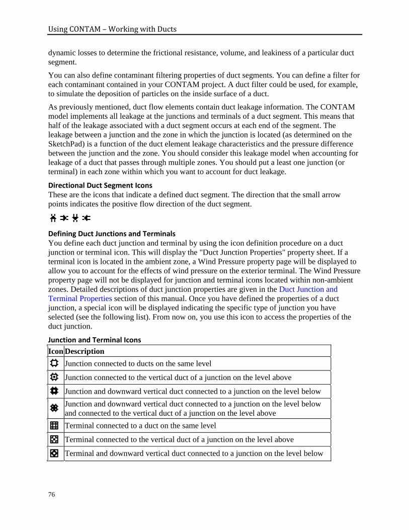
Using CONTAM – Working with Ducts
76
dynamic losses to determine the frictional resistance, volume, and leakiness of a particular duct
segment.
You can also define contaminant filtering properties of duct segments. You can define a filter for
each contaminant contained in your CONTAM project. A duct filter could be used, for example,
to simulate the deposition of particles on the inside surface of a duct.
As previously mentioned, duct flow elements contain duct leakage information. The CONTAM
model implements all leakage at the junctions and terminals of a duct segment. This means that
half of the leakage associated with a duct segment occurs at each end of the segment. The
leakage between a junction and the zone in which the junction is located (as determined on the
SketchPad) is a function of the duct element leakage characteristics and the pressure difference
between the junction and the zone. You should consider this leakage model when accounting for
leakage of a duct that passes through multiple zones. You should put a least one junction (or
terminal) in each zone within which you want to account for duct leakage.
Directional Duct Segment Icons These are the icons that indicate a defined duct segment. The direction that the small arrow
points indicates the positive flow direction of the duct segment.
Defining Duct Junctions and Terminals You define each duct junction and terminal by using the icon definition procedure on a duct
junction or terminal icon. This will display the "Duct Junction Properties" property sheet. If a
terminal icon is located in the ambient zone, a Wind Pressure property page will be displayed to
allow you to account for the effects of wind pressure on the exterior terminal. The Wind Pressure
property page will not be displayed for junction and terminal icons located within non-ambient
zones. Detailed descriptions of duct junction properties are given in the Duct Junction and
Terminal Properties section of this manual. Once you have defined the properties of a duct
junction, a special icon will be displayed indicating the specific type of junction you have
selected (see the following list). From now on, you use this icon to access the properties of the
duct junction.
Junction and Terminal Icons
Icon Description
Junction connected to ducts on the same level
Junction connected to the vertical duct of a junction on the level above
Junction and downward vertical duct connected to a junction on the level below
Junction and downward vertical duct connected to a junction on the level below
and connected to the vertical duct of a junction on the level above
Terminal connected to a duct on the same level
Terminal connected to the vertical duct of a junction on the level above
Terminal and downward vertical duct connected to a junction on the level below
Using CONTAM – Working with Ducts
77
3.7.6 Duct Segment Properties
This section provides detailed descriptions of the specific duct segment properties. Each of the
following subsections are the context-sensitive help topics that you can access by pressing F1
when working with property pages of the "Duct Segment Properties" property sheet.
Duct Segment - Flow Element Properties
Duct Segment Number: This is the number that appears in the status bar when you highlight a
duct segment icon. ContamW automatically assigns this number to each duct segment once they
are defined. This number could change as you add and remove duct segments to or from a
project. Each time you save a project, the duct segment numbers are reassigned. Numbers are
assigned beginning on the top level, starting from the upper-left corner of the SketchPad, moving
left-to-right and top-to-bottom of the SketchPad.
Duct Flow Element Name: You may select a previously defined airflow element from those
contained in the Name list. Click the "New Element" button to define a new airflow element. To
view or modify airflow element data click the "Edit Element" button. Every duct segment must
have an airflow element associated with it. This field may not be left blank.
Model Summary: This summarizes the information associated with the duct flow element
currently displayed in the Name field.
Duct Segment - Segment Properties
Segment Data:
Duct segment length: Enter the length of the duct segment. This will be used along with the
cross-sectional area to determine the volume of the duct segment.
Sum of loss coefficients: This is the sum of all dynamic loss coefficients due to junction
losses and all fittings in the segment. This term only applies to the Darcy-Colebrook duct
flow element model (see Ducts in the Airflow Analysis section).
Positive Flow Direction: In the case of fans and backdraft dampers it is necessary to know
which direction is defined as positive. The arrows represent the positive direction for
pressure drop and airflow.
Color: You can set the color of each segment individually here, or you can use the automated
Duct System Coloring Tool to color sections of ducts related to forced flow elements within the
duct system. You access the Duct System Coloring Toolvia the ViewDuct Coloring... menu
command (See Drawing Ducts).
Segment Summary Information: This field displays information about the selected duct flow
element.
Duct Segment - Schedule Properties
The schedule value will operate proportionally on various items depending on the type of flow
element associated with the duct segment. For most flow elements, it will operate directly on the
flow rate. For the fan performance curve element it will act as the ratio of the fan operating speed
to the fan off operating speed. The schedule can not be applied to the Darcy-Colebrook element,
and the schedule properties will be disabled in the ContamW interface for this type of flow
element.
Using CONTAM – Working with Ducts
78
Schedule: If there are previously defined schedules within the current project, you may select
one from the Name list. Click the "New Schedule" button to define a new schedule. To view or
modify an existing schedule click the "Edit Schedule" button. Setting this field to <none>
indicates no schedule. (See Working with Schedules)
CVF/DVF Control: Values from either a CVF or DVF file can be used in place of the above
Schedule (read about CVF and DVF controls in the Control Element Types section). This
enables using these control element types without having to draw/define an associated control
network. The associated radio buttons "Use Neither", "Use CVF" and "Use DVF" are used to
select the desired control method. Select the heading name from the associated "Name" drop
down box that will display the headings of either the CVF or DVF file as per the aforementioned
radio button selection.
Control Status: This will display the current method of control: Schedule, direct CVF, direct
DVF or Control Network. If an actuator of a control network on the SketchPad is associated with
the scheduled item then it will take precedence over the Schedule and CVF/DVF Control. If
either the "Use CVF" or "Use DVF" radio button is selected then CVF or DVF will take
precedence over an associated schedule.
Duct Segment - Filter Properties
Filter: You may select a previously defined filter from those contained in the associated Name
list. Click the "New Filter" button to define a new filter. Click the "Edit Filter" button to view or
modify existing filter data. Setting this field to <none> indicates no filter for this airflow path.
(See Contaminant Filters under Working with Contaminants)
Duct Flow Element - Shape, Size and Leakage
Duct Shape: You can implement several different shapes of ducts including: round, rectangular,
oval or other. Select the shape you want and the appropriate dimensions will be made available
for you to enter under the Duct Dimension parameters.
Duct Dimensions: The data entered here is dependent on the duct shape. For circular ducts, the
diameter is the only parameter needed. Rectangular ducts require you to enter the width and
height, and oval ducts require you to input the major and minor dimensions. The other option
allows you to enter a perimeter and a flow area to define the dimensions for a duct of any other
shape.
Leakage: Leakage of air between the duct and the surrounding zone may be described in terms
of a leakage rate (per unit surface area of duct segment) at a given pressure or by use of the
leakage classification. If you enter a leakage rate and a pressure difference, the value for the
leakage class is automatically calculated by ContamW and placed in the "Leakage Class" field.
Similarly, if you input a leakage class, a default value of 250 Pa is used for the pressure
difference, and a leakage rate will be calculated based on the pressure difference and the leakage
class you entered. See [ASHRAE 2005 Chapter 35]

Using CONTAM – Working with Ducts
79
Duct Flow Element Types
This is a list of available duct flow elements or mathematical models that provide the
relationship between airflow and pressure difference for duct segments. See Airflow Analysis in
the Theoretical Background section of the manual for mathematical details.
Darcy-Colebrook Model The most common model to use for CONTAM duct systems is the Darcy-Weisbach relation and
Colebrook's natural roughness function.
Darcy-Colebrook Model
Powerlaw Models Three versions of the powerlaw model are included:
1. Orifice resistance model
2. Resistance: F = C(P)^n (mass flow)
3. Resistance: Q = C(P)^n (volume flow)
Forced Flow Models Three types of forced flow models are included:
1. Fan - performance curve
2. Constant mass flow
3. Constant volume flow
Backdraft Damper Models The Backdraft Damper models make it possible to model a feature (e.g. a smoke control damper)
that has different flow resistances depending on the direction of the pressure drop, with greatly
reduced (or zero) flow in one direction.
1. Backdraft Damper: F = C(P)^n (mass flow)
2. Backdraft Damper: Q = C(P)^n (volume flow)
Cubic Spline Flow Models These models provide the ability to create user-defined duct flow elements based on a set of data
points to which a cubic spline curve is fit. There are four versions that relate either mass flow or
volume flow to pressure difference across the flow element (or vice versa). The cubic spline
curve fit insures that the relationship between flow and pressure is differentiable as required by
the CONTAM airflow solver.
1. F vs P: Mass flow rate as a function of Pressure difference
2. Q vs P: Volume flow rate as a function of Pressure difference
3. P vs F: Pressure difference as a function of Mass flow rate
4. P vs Q: Pressure difference as a function of Volume flow rate
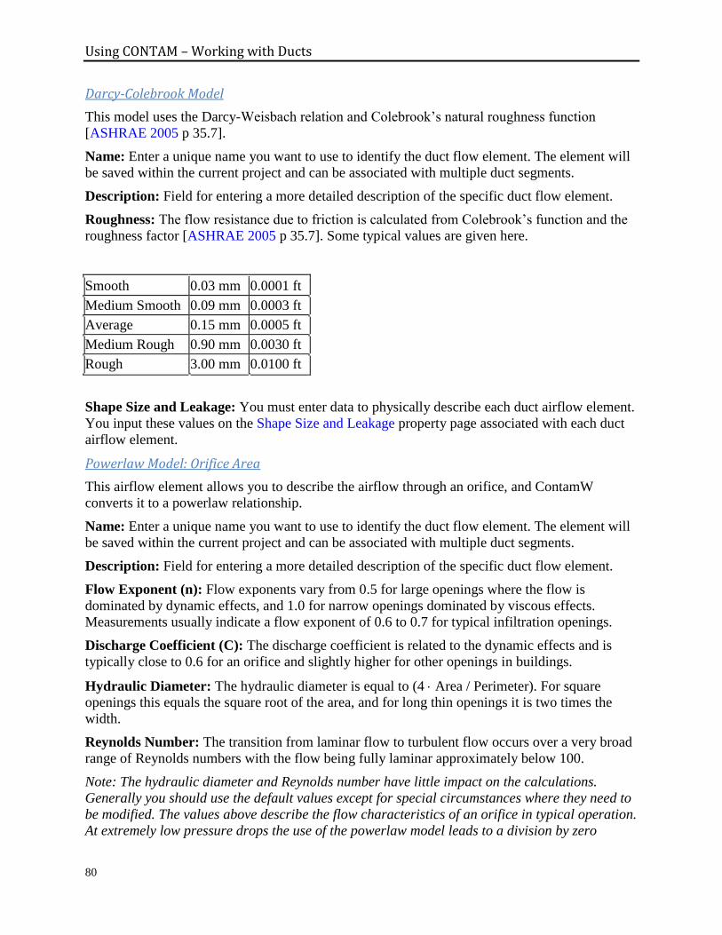
Using CONTAM – Working with Ducts
80
Darcy-Colebrook Model
This model uses the Darcy-Weisbach relation and Colebrook’s natural roughness function
[ASHRAE 2005 p 35.7].
Name: Enter a unique name you want to use to identify the duct flow element. The element will
be saved within the current project and can be associated with multiple duct segments.
Description: Field for entering a more detailed description of the specific duct flow element.
Roughness: The flow resistance due to friction is calculated from Colebrook’s function and the
roughness factor [ASHRAE 2005 p 35.7]. Some typical values are given here.
Smooth 0.03 mm 0.0001 ft
Medium Smooth 0.09 mm 0.0003 ft
Average 0.15 mm 0.0005 ft
Medium Rough 0.90 mm 0.0030 ft
Rough 3.00 mm 0.0100 ft
Shape Size and Leakage: You must enter data to physically describe each duct airflow element.
You input these values on the Shape Size and Leakage property page associated with each duct
airflow element.
Powerlaw Model: Orifice Area
This airflow element allows you to describe the airflow through an orifice, and ContamW
converts it to a powerlaw relationship.
Name: Enter a unique name you want to use to identify the duct flow element. The element will
be saved within the current project and can be associated with multiple duct segments.
Description: Field for entering a more detailed description of the specific duct flow element.
Flow Exponent (n): Flow exponents vary from 0.5 for large openings where the flow is
dominated by dynamic effects, and 1.0 for narrow openings dominated by viscous effects.
Measurements usually indicate a flow exponent of 0.6 to 0.7 for typical infiltration openings.
Discharge Coefficient (C): The discharge coefficient is related to the dynamic effects and is
typically close to 0.6 for an orifice and slightly higher for other openings in buildings.
Hydraulic Diameter: The hydraulic diameter is equal to (4 Area / Perimeter). For square
openings this equals the square root of the area, and for long thin openings it is two times the
width.
Reynolds Number: The transition from laminar flow to turbulent flow occurs over a very broad
range of Reynolds numbers with the flow being fully laminar approximately below 100.
Note: The hydraulic diameter and Reynolds number have little impact on the calculations.
Generally you should use the default values except for special circumstances where they need to
be modified. The values above describe the flow characteristics of an orifice in typical operation.
At extremely low pressure drops the use of the powerlaw model leads to a division by zero
Using CONTAM – Working with Ducts
81
during the network solution process. ContamX avoids this problem by changing to a linear
model in this region. The model is based conceptually on the flow changing from turbulent to
laminar at very low pressures. The Hydraulic diameter and Reynolds number are used to
determine a point where the model changes from the powerlaw to linear.
Shape Size and Leakage: You must enter data to physically describe each duct airflow element.
You input these values on the Shape Size and Leakage property page associated with each duct
airflow element.
Powerlaw Model: F=C(P)^n
This airflow element allows you to directly enter the coefficients C and n for the mass flow
version of the powerlaw model.
Name: Enter a unique name you want to use to identify the duct flow element. The element will
be saved within the current project and can be associated with multiple duct segments.
Description: Field for entering a more detailed description of the specific duct flow element.
Flow Coefficient (C): The coefficients may only be expressed in SI units due to the conversion
method used. Use the following conversion to convert from IP units to SI units.
Flow Exponent (n): Flow exponents vary from 0.5 for large openings where the flow is
dominated by dynamic effects, and 1.0 for narrow openings dominated by viscous effects.
Measurements usually indicate a flow exponent of 0.6 to 0.7 for typical infiltration openings.
Shape Size and Leakage: You must enter data to physically describe each duct airflow element.
You input these values on the Shape Size and Leakage property page associated with each duct
airflow element.
Powerlaw Model: Q=C(P)^n
This airflow element allows you to directly enter the coefficients C and n for the volumetric flow
version of the powerlaw model.
Name: This is the name you give to this airflow element. This name must be unique within a
project.
Description: Field for entering a more detailed description of the specific duct flow element.
Flow Coefficient (C): The coefficients may only be expressed in SI units due to the conversion
method used. Use the following conversion to convert from IP units to SI units.
Flow Exponent (n): Flow exponents vary from 0.5 for large openings where the flow is
dominated by dynamic effects, and 1.0 for narrow openings dominated by viscous effects.
Measurements usually indicate a flow exponent of 0.6 to 0.7 for typical infiltration openings.
Using CONTAM – Working with Ducts
82
Shape Size and Leakage: You must enter data to physically describe each duct airflow element.
You input these values on the Shape Size and Leakage property page associated with each duct
airflow element.
Fan Model: Performance Curve
This airflow element allows you to create a fan based on a fan performance curve. You provide
ContamW with a set of pressure rise and airflow rate data points, and ContamW performs a
polynomial curve fit to the data point.
Name: Enter a unique name you want to use to identify the duct flow element. The element will
be saved within the current project and can be associated with multiple duct segments.
Fan off conditions: These values specifies how the fan is modeled when the speed of the fan is
insufficient to provide a flow.
Cut-off Ratio: The fan speed ratio is the actual speed (RPM) of the fan divided by the rated
speed of the fan (fan is defined for a speed ratio of 1.0). When the fan speed ratio is below the
specified cut-off ratio the fan is modeled as a simple orifice based on the "equivalent orifice"
defined for this fan element. During a simulation, ContamX obtains the actual ratio from the
control value being applied (in the form of a schedule or control signal) to the airflow path with
which this fan element is associated and compares it to the cut-off ratio. See Chapter 18 Fans in
[ASHRAE 2004].
Equivalent Orifice: The size of the orifice used to model the fan opening when the schedule
or control value drops below the specified cut-off ratio.
Description: Field for entering a more detailed description of the specific airflow element.
Fan Performance Data: Click the "Edit Fan Curve Data" to input/modify the fan curve for this
duct flow element. A detailed explanation of this data is given in the Fan Performance Data
section under Working with Airflow Paths.
Shape Size and Leakage: You must enter data to physically describe each duct airflow element.
You input these values on the Shape Size and Leakage property page associated with each duct
airflow element.
Fan Model: Constant Mass Flow
This airflow element allows you to describe the airflow through a duct as a constant mass airflow
rate.
Name: Enter a unique name you want to use to identify the duct flow element. The element will
be saved within the current project and can be associated with multiple duct segments.
Description: Field for entering a more detailed description of the specific duct flow element.
Design (max) Flow: Enter the maximum mass flow rate. You can use the duct segment schedule
to modify this value.
Shape Size and Leakage: You must enter data to physically describe each duct airflow element.
You input these values on the Shape Size and Leakage property page associated with each duct
airflow element.
Using CONTAM – Working with Ducts
83
Fan Model: Constant Volume Flow
This duct flow element allows you to describe the airflow through a duct as a constant
volumetric flow rate. The design flow rate you specify is in terms of standard air. CONTAM
uses a value of 1.204 kg/m3 based on conditions specified by ASHRAE for dry air: 101.325 kPa
and 20ºC [Chapter 18 of ASHRAE 2004]. Therefore, if actual conditions during simulation do
not match these standard conditions, the results will differ from specified flow due to differences
in air density.
Name: Enter a unique name you want to use to identify the duct flow element. The element will
be saved within the current project and can be associated with multiple duct segments.
Description: Field for entering a more detailed description of the specific duct flow element.
Design (max) Flow: Enter the maximum volume flow rate. You can use the duct segment
schedule to modify this value.
Shape Size and Leakage: You must enter data to physically describe each duct airflow element.
You input these values on the Shape Size and Leakage property page associated with each duct
airflow element.
Backdraft Damper: Q=C(P)^n
This is the volumetric flow version of the Backdraft Damper duct flow element. The Backdraft
Damper models make it possible to model a feature (e.g. a smoke control damper) that has
different flow resistances depending on the direction of the pressure drop, with greatly reduced
(or zero) flow in one direction.
Name: Enter a unique name you want to use to identify the duct flow element. The element will
be saved within the current project and can be associated with multiple duct segments.
Description: Field for entering a more detailed description of the specific duct flow element.
Pressure Difference: Enter a flow coefficient and exponent for both the positive and negative
flow directions of the duct segment. P>0 refers to the pressure difference across the flow
element that would lead to an airflow in the positive flow direction (See Duct Segment
Properties ) and P<0 would lead to a flow in the opposite direction.
Flow Coefficients: The coefficients may only be expressed in SI units due to the conversion
method used. Use the following conversion to convert from IP units to SI units.
Flow Exponents: Flow exponents vary from 0.5 for large openings where the flow is
dominated by dynamic effects, and 1.0 for narrow openings dominated by viscous effects.
Measurements usually indicate a flow exponent of 0.6 to 0.7 for typical infiltration openings.
Shape Size and Leakage: You must enter data to physically describe each duct airflow element.
You input these values on the Shape Size and Leakage property page associated with each duct
airflow element.
Using CONTAM – Working with Ducts
84
Backdraft Damper: F=C(P)^n
This is the mass flow version of the Backdraft Damper duct flow element. The Backdraft
Damper models make it possible to model a feature (e.g. a smoke control damper) that has
different flow resistances depending on the direction of the pressure drop, with greatly reduced
(or zero) flow in one direction.
Name: Enter a unique name you want to use to identify the duct flow element. The element will
be saved within the current project and can be associated with multiple duct segments.
Description: Field for entering a more detailed description of the specific duct flow element.
Pressure Difference: Enter a flow coefficient and exponent for both the positive and negative
flow directions of the duct segment. P>0 refers to the pressure difference across the flow
element that would lead to an airflow in the positive flow direction (See Duct Segment
Properties ) and P<0 would lead to a flow in the opposite direction.
Flow Coefficients: The coefficients may only be expressed in SI units due to the conversion
method used. Use the following conversion to convert from the IP units to SI units.
Flow Exponents: Flow exponents vary from 0.5 for large openings where the flow is
dominated by dynamic effects, and 1.0 for narrow openings dominated by viscous effects.
Measurements usually indicate a flow exponent of 0.6 to 0.7 for typical infiltration openings.
Shape Size and Leakage: You must enter data to physically describe each duct airflow element.
You input these values on the Shape Size and Leakage property page associated with each duct
airflow element.
Duct Junction and Terminal Properties
This section provides detailed descriptions of the specific duct junction and terminal properties.
The following sections are the context-sensitive help topics that you can access by pressing F1
when working with property pages of the "Duct Junction Properties" property sheet.
Duct Junction and Terminal - Junction Properties
Junction Number: This number is automatically generated by ContamW for identification
purposes and is unique to each junction. ContamW will renumber junctions and terminals when
saving a project if you have added or removed any junctions or terminals. These icons are
numbered starting at the top level in the upper left hand corner of the SketchPad moving left to
right and down the SketchPad then proceeding down through each level in the same manner.
Relative Elevation & Temperature: The elevation and temperature of the junction are used to
determine how the duct flow responds to and influences the building stack effect. Enter the
height of the midpoint of the junction or terminal point relative to the current building level.
Enter the temperature you wish the junction or terminal to use during simulation.
Note that you can have ContamX calculate duct temperatures when performing simulations using
the 1D Duct Model with the Short Time Step Method. See Contaminant Numerics Properties in
the Working with Simulations section.
Using CONTAM – Working with Ducts
85
Junction: If you are creating a junction that connects two duct segments, then select the type of
connection to create here. Items will be enabled/disabled depending on the valid connection
types.
Define Downward Duct: You define vertical duct segments as downward running ducts
accessed via the duct junction at the top of the downward segment. Press the "Define
Downward Duct" button to define vertical segments. The SketchPad duct icons that are
connected to the defined vertical duct will change to indicate the type of vertical connections
associated with the junction, i.e., connected downward, upward or both (see Junction and
Terminal Icons).
Terminal: If you are creating a terminal at the end of a duct segment, then select the type of
connection to create here. Items will be enabled/disabled depending on the valid connection
types.
Location: Enter the absolute X and Y coordinates and units for the selected junction. The Z
coordinate will be taken as the Relative Height of the junction with respect to the building level
on which the junction is located.
These values are required for terminals located in the Ambient zone when using a Wind Pressure
and Contaminant (WPC) file (see Working with WPC Files) or for junctions and terminals
located within a 1D convection/diffusion zone (see 1D Zone Data). These coordinates will be
verified by ContamW against a WPC file or the axis of the 1D zone in which the junction or
terminal is located. This verification will be performed automatically when you select either the
Run Simulation or Create a ContamX Input File command from the Simulation menu.
Duct Junction and Terminal - Wind Pressure Properties
This set of properties is available only for those terminals that are located in the ambient zone
and thus potentially subject to wind effects.
Wind Pressure Option: There are three wind pressure options for duct terminals located in an
ambient zone:
1. No wind pressure
2. Constant pressure
3. Pressure dependent on wind speed and direction
When you select one of the above options, the following data entry options that correspond to the
wind pressure option that you selected will be made available for your input.
Constant Pressure Data: Enter a constant wind pressure (wind speed and direction
independent).
Variable Pressure Data: Variable wind pressures are computed from the product of the
following three parameters:
1. The dynamic pressure of the wind at some reference height.
ContamX will determine this pressure based on either the steady state wind data (See
Wind Properties) or the transient wind data from a weather file (See Defining Transient
Weather and Wind).
2. A coefficient accounting for local terrain effects (Wind Pressure Modifier).
Using CONTAM – Working with Ducts
86
3. A pressure coefficient accounting for relative wind direction (Wind Pressure Profile).
Wind Pressure Modifier: CONTAM uses this value to account for differences between
wind velocity profiles at the building site and that at a measurement location, e.g. an airport
weather station (See Working with Weather and Wind). CONTAM only requires this value if
you are implementing Variable Wind Pressure for an airflow path. ContamW will provide a
default value for this based on the data entered via the Weather and Wind Parameters
Property Page or you can override the default value for a particular airflow path.
Wall Azimuth Angle: Enter the direction the wall faces (clockwise from north).
Profile: The wind pressure profile accounts for the wind direction effects. You may select a
previously defined wind pressure profile from those contained in the Name list. Click the
"New Profile" button to define a new wind pressure profile. To view or modify wind pressure
profile data, click the "Edit Profile" button. After you press the "New Profile" or "Edit
Profile" button, the Wind Pressure Profile page will be displayed with a graphical
representation of the profile.
Duct Junction and Terminal - Terminal Properties
Prior to CONTAM 2.4, duct terminals merely provided connectivity of the duct network to zones
and did not have user-defined properties associated with them. Beginning with CONTAM 2.4,
duct terminals have been revised to be more like duct flow segments, having geometric
properties, loss coefficients and flow balancing capabilities.
Terminal flow is determined by the effective loss coefficient (Ce) of the terminal. Ce is determined
during simulation by the combination of the Terminal Loss Coefficient (Ct), Balance Coefficient
(Cb) and schedule value or control signal (Sc). As implied here, terminals can now be acted upon
via the control network or scheduled to allow Ce to range between (Ct + Cb) for a control signal
of 1.0 and a very large loss coefficient that essentially reduces the flow to zero for a control
signal of 0.0. (See Ducts in the Airflow Analysis section of the Theoretical Background).
You can use the terminal properties to define the loss characteristics of a duct terminal to be used
during simulation; to provide geometric data that will enable ContamW to provide you with
more meaningful flow velocities at the terminal; and to define duct balancing properties that
CONTAM can use to establish user-defined design airflow rates at the duct terminals. After
setting the design conditions below, you can have CONTAM perform the duct balancing by
selecting the Duct Balance airflow simulation method of the Run Control Properties.
Junction Number: This number is automatically generated by ContamW for identification
purposes and is unique to each junction. ContamW will renumber junctions and terminals when
saving a project if you have added or removed any junctions or terminals. These icons are
numbered starting at the top level in the upper left hand corner of the SketchPad moving left to
right and down the SketchPad then proceeding down through each level in the same manner.
Terminal Data: These properties are the characteristic data that describe the terminal itself
regardless of whether it is balanced or not.
Terminal Loss Coefficient: Characteristic loss coefficient of the terminal. The default value
is 0.125. See chapter 35 of [ASHRAE 2005] and the Duct Fitting Database [ASHRAE 2002]
for data on dynamic losses in duct fittings.
Using CONTAM – Working with Ducts
87
NOTE: Earlier versions of CONTAM (version 2.2 and earlier) did not implement loss
coefficients at the terminals. When updating these earlier versions of CONTAM PRJ files,
terminal loss coefficients will be applied to all terminals. For those terminals whose adjacent
duct segments had loss coefficients associated with them, half of the segment loss coefficient
will be applied to the terminal and half to the adjacent segment. All other terminals will be
provided with a minimum allowable value of 0.001, thus effecting a very small loss at the
terminal to provide consistency with terminal flow results prior to the conversion.
Free Face Area: This is the total minimum area of the openings in the air outlet or inlet
through which air can pass. This area will be used to calculate the velocity from the airflow
rate at the terminal when displaying simulation results on the SketchPad.
Duct Area: The area of the duct to which the terminal is connected. Typically, this would be
the same area as the duct segment just downstream/upstream from the supply/return air
terminal. This value is used during simulation to determine the airflow rate through the
terminal.
Balancing Data: These properties are used for the automated duct balancing capabilities
implemented in CONTAM version 2.4. This feature will enable you to select a set of duct
terminals for which you provide design airflow rates and have ContamX calculate loss
coefficients that will enable the associated supply fan to provide the design flow rate.
Balance Terminal: Check this box if you would like ContamX to include this terminal in the
duct balancing procedure.
Design Flow Rate: Provide the design airflow rate for which you want ContamX to
determine a Balance Loss Coefficient. Specify positive values for supply flow terminals, i.e.
airflow from the duct system to the zone in which the terminal is located, and negative values
for return air terminals.
Max Balance Coefficient: Provide a maximum value for the Balance Loss Coefficient
below. This will be used to provide warning information if the Balance Loss Coefficient
determined by the automated balancing procedure of ContamX exceeds this value.
Balance Loss Coefficient: This is the loss coefficient determined via the automated
balancing procedure of ContamX. You can also modify it "manually." As noted above, this
value will be used to determine the effective loss coefficient (Ce) for the terminal.
Filter and Schedule
Junctions and terminals differ with respect to Filters and Schedules. Junctions can not have
filters associated with them and only the temperature of the junction can be scheduled or
controlled. Beginning with CONTAM version 2.4, terminals can be both filtered and scheduled.
The terminal temperature and loss coefficient can be scheduled (or controlled), although only
one type of schedule can be applied at a time.
Filter: You may either create, edit or delete the filter associated with this terminal. Creating a
new filter or modifying an existing one will display the Filter Properties dialog box. Use this
dialog box to create and edit filter elements as needed. For an explanation of contaminant filters
see Contaminant Filters in the Using CONTAM section of the manual.
Schedule: As of CONTAM version 2.4, terminals consist of both a duct segment and a terminal
junction during simulation. Each of these are schedulable items. You can select to schedule
Using CONTAM – Working with Ducts
88
either the Loss coefficient of the segment or the Temperature of the junction. The list of
schedules will contain those types (unitless or temperature) of schedules that exist in the project.
If there are previously defined schedules within the current project, you may select one from the
Name list. Click the "New Schedule" button to define a new schedule. To view or modify an
existing schedule click the "Edit Schedule" button. Setting this field to <none> indicates no
schedule. (See Working with Schedules)
CVF/DVF Control: Values from either a CVF or DVF file can be used in place of the above
Schedule (read about CVF and DVF controls in the Control Element Types section). This
enables using these control element types without having to draw/define an associated control
network. The associated radio buttons "Use Neither", "Use CVF" and "Use DVF" are used to
select the desired control method. Select the heading name from the associated "Name" drop
down box that will display the headings of either the CVF or DVF file as per the aforementioned
radio button selection.
Control Status: This will display the current method of control: Schedule, direct CVF, direct
DVF or Control Network. If an actuator of a control network on the SketchPad is associated with
the scheduled item then it will take precedence over the Schedule and CVF/DVF Control. If
either the "Use CVF" or "Use DVF" radio button is selected then CVF or DVF will take
precedence over an associated schedule.
Balancing Duct Systems
In CONTAM you can balance duct systems yourself by providing balance points, e.g., orifice
flow elements, at desired locations, or you can have CONTAM balance the system for you.
Versions of CONTAM prior to version 2.4 required you to balance the system manually by
adjusting the resistance of duct flow elements or local loss coefficients at desired balancing
points. Beginning with version 2.4, CONTAM provides the ability to automatically balance duct
systems using CONTAM duct terminals. See Duct Junction and Terminal - Terminal Properties
and Working with Simulations.
Automated Duct Balancing Procedure Automated duct balancing is another mode of simulation in ContamX. When you initiate a
balance, ContamW will perform a pre-simulation check on the PRJ file and, if the check is
successful, save the PRJ file and execute ContamX. ContamX will perform its own set of pre-
balance checks to determine if a valid set of conditions has been defined. If this check is
successful, then the automated balancing mode of ContamX will be initiated. If the pre-check of
ContamX is unsuccessful, an error message will be displayed indicating the nature of the pre-
check failure.
The automated procedure establishes relationships between fan elements and duct terminals by
first performing a steady state airflow simulation for the entire building system as defined, i.e.,
duct balance coefficients having not yet been modified. If there are no errors in the system
configuration, it then replaces fan elements with constant flow balancing fans, initializes fan
flow rates to the summation of design flows of associated terminals (the minimum flow required
for balancing), performs an airflow simulation, and checks for convergence of the duct balance
by comparing calculated airflows with design airflows for all balance terminals. If convergence
is not met, then the balance coefficients are adjusted (only increased) and the procedure is
repeated until either convergence or the maximum number of iterations are performed. Upon
Using CONTAM – Working with Ducts
89
completion of the balancing, ContamX will create a simulation results file (SIM file) that
contains the calculated airflow results of the balanced system (see items 0 and 1 below).
The automated balance procedure generates a duct balance result file which has the same name
as the project file but having the BAL extension. The contents of the balance report file will vary
depending on the results of the automated balance procedure (See Results Files in the Working
with Results section).
The basic steps to use the duct balancing feature are outlined below:
Draw duct system – define segments, terminals and fans. Be sure to use separate fan flow
elements for each fan, as the balance procedure may need to adjust the flow rates
individually to achieve desired results. In order to obtain as realistic and reasonable results
as possible, you should provide known loss coefficients at each terminal and junction
throughout the system. Otherwise, the balancing procedure might not produce desired
static pressures within the system – although design flows will be achieved.
Designate balancing terminals and set design airflow rates for each.
Select airflow simulation balance procedure and run simulation.
Observe feedback from balance procedure. There are six possible results. If the one of the
first two results (Success or Non-convergence) is obtained, a simulation results file will be
created that contains the airflow rates calculated based on the calculated balance
coefficients. If one of the four error results is obtained, then the simulation results are for
the pre-balance steady state calculation of the system as defined. The following list
provides the six different outcomes of the balance and their associated completion code as
it will appear in the first line of the duct balance results file.
0. Success: The balance procedure completed successfully. You will be prompted to copy
balance coefficients to terminals and balance flow rates to constant flow fan elements when
using such elements to model the fan. Once you have responded to the prompts, you can
review the results of the balance on the SketchPad. Airflow rates from the terminals will be
displayed via the SketchPad results display method. Balance coefficients will not be saved
until you save the project, so you can maintain the original pre-balance file by saving the
post-balance file under a new name.
Performance curve fan elements are treated differently from constant flow fan elements,
because they can not be directly modified to provide the balance flow rates. If using fan
curve elements, consult the balance report file for setting the fan speed ratio to provide
design flow rates. Use the value reported to provide a speed ratio via a control signal or
schedule value to achieve the balance flow with the fan. If a value of 0.0 is reported, then the
fan curve is not capable of providing the desired flow via a reasonable fan speed ratio and
pressure rise. In this case it is likely that a different fan should be used.
1. Non-convergence: The balance procedure was not able to obtain the desired balance flow
rates for all of the terminals within the preset number of iterations. You can choose to accept
the calculated balance coefficients and run the balance procedure again with the modified
coefficients as initial values. The balance report file will provide a relative flow coefficient
equal to the calculated flow rate divided by the design flow rate.
Using CONTAM – Working with Ducts
90
2. Error: No terminals to balance: There are no terminals having the Balance Terminal
option selected. Be sure to check the Balance Terminal check box to designate terminals to
be balanced.
3. Error: Invalid flow direction(s): This error occurs when the balance terminals associated
with a single fan have opposing design flow directions. Be sure the design flow direction of
all terminals matches that of the associated fan: positive design flow rates are out of the
terminal into the zone in which the terminal is located, and negative design flow rates are
into the terminal from the zone. The fan flow direction is user-selectable via the duct segment
icon of the associated fan.
4. Error: Failed to terminate link(s) at a fan: This error occurs when one or more balance
terminals can not be traced back through the duct system (links) to a forced flow element
(fan) within the duct system.
5. Error: Fan system includes supply and return terminal: This error occurs when a given fan
has balance terminals both upstream and downstream of the fan. Be sure to only attempt to
balance terminals on either the upstream or downstream side of a fan.
DUCT BALANCING NOTES: Duct balancing is performed under consideration of the entire building system. When the
airflow calculation is performed during each iteration of the balancing procedure, the
resistances between zones are included. Interzone resistances that are relatively high can
impact the balancing results.
During duct balancing, all junction temperatures are set to 20 ºC. Ambient conditions are
established by the steady state weather data with the exception that wind is set to 0 m/s.

Using CONTAM – Working with Controls
91
3.8 WORKING WITH CONTROLS
Controls allow the characteristics of one building element to be modified during transient
simulations in response to a change in characteristics of another building element. You can also
use controls to simply monitor building performance by polling building components for values
and logging them to a control log file during a simulation.
Controls include sensors, links, modifiers and actuators. Sensors are control elements that are
used to obtain a value, calculated during simulation, of a building component and then provide it
to a control network. You can use sensors to obtain contaminant concentrations and temperatures
of zones, duct junctions and duct terminals and to obtain pressure differences and airflow rates of
airflow paths, duct segments and duct terminals. You can use actuators to control schedulable
items including airflow paths, duct segments, junctions and terminals, simple air-handling
systems, and contaminant source/sinks. Note that actuator input to a controlled building
component overrides schedules associated with the component.
The connection between sensors and other nodes in a control network are made up of control
links. Control modifiers are nodes within the control network that are used to change or modify
their input signals. Control actuators are used to modify various characteristics of building
components based on control signals obtained from sensors and even modified by signal
modifiers. For example, a sensor can be used to obtain a contaminant concentration within a
zone, and a proportional control actuator can be used to adjust supply airflow through a supply
airflow path into the zone based on the sensed concentration.
3.8.1 Control Elements
A control network can consist of many different control nodes, each of which is defined by a
control element. There are several different types of control elements provided, such as a report
element, that can be used to convert dimensionless sensor values to engineering units;
mathematical elements to perform simple mathematical and logical operations on input signals;
and classical control elements such as proportional/integral, band and limit controls. There is a
phantom control element that can be used to reference an existing control node, which is
convenient for linking nodes that may be on different levels of a building or simply too far apart
to conveniently draw a physical link. Each of these element types is described in detail in the
Control Element Types section. While every node in the control network must refer to a single
control element, multiple nodes can refer to the same control element using the phantom
node/control element.
Collections of control elements can be grouped into Control Super Elements, which can be
stored in CONTAM Library files and shared within and between projects. Super elements can
reduce the amount of drawing of repetitive control logic and enable the creation of custom
reusable sensors and control algorithms.
3.8.2 Drawing Controls
You draw controls using the links drawing tools previously described in the "Working with the
SketchPad" section. When you finalize the drawing of a set of control links, the appropriate icons
will be placed upon the SketchPad depending on where the link originates and where it
terminates. For example, if you begin drawing a control link directly on a zone icon, a sensor
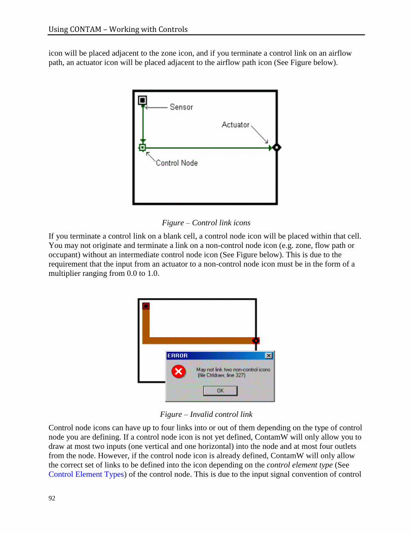
Using CONTAM – Working with Controls
92
icon will be placed adjacent to the zone icon, and if you terminate a control link on an airflow
path, an actuator icon will be placed adjacent to the airflow path icon (See Figure below).
Figure – Control link icons
If you terminate a control link on a blank cell, a control node icon will be placed within that cell.
You may not originate and terminate a link on a non-control node icon (e.g. zone, flow path or
occupant) without an intermediate control node icon (See Figure below). This is due to the
requirement that the input from an actuator to a non-control node icon must be in the form of a
multiplier ranging from 0.0 to 1.0.
Figure – Invalid control link
Control node icons can have up to four links into or out of them depending on the type of control
node you are defining. If a control node icon is not yet defined, ContamW will only allow you to
draw at most two inputs (one vertical and one horizontal) into the node and at most four outlets
from the node. However, if the control node icon is already defined, ContamW will only allow
the correct set of links to be defined into the icon depending on the control element type (See
Control Element Types) of the control node. This is due to the input signal convention of control
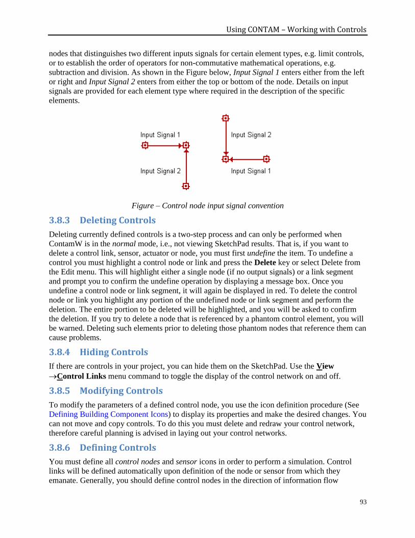
Using CONTAM – Working with Controls
93
nodes that distinguishes two different inputs signals for certain element types, e.g. limit controls,
or to establish the order of operators for non-commutative mathematical operations, e.g.
subtraction and division. As shown in the Figure below, Input Signal 1 enters either from the left
or right and Input Signal 2 enters from either the top or bottom of the node. Details on input
signals are provided for each element type where required in the description of the specific
elements.
Figure – Control node input signal convention
3.8.3 Deleting Controls
Deleting currently defined controls is a two-step process and can only be performed when
ContamW is in the normal mode, i.e., not viewing SketchPad results. That is, if you want to
delete a control link, sensor, actuator or node, you must first undefine the item. To undefine a
control you must highlight a control node or link and press the Delete key or select Delete from
the Edit menu. This will highlight either a single node (if no output signals) or a link segment
and prompt you to confirm the undefine operation by displaying a message box. Once you
undefine a control node or link segment, it will again be displayed in red. To delete the control
node or link you highlight any portion of the undefined node or link segment and perform the
deletion. The entire portion to be deleted will be highlighted, and you will be asked to confirm
the deletion. If you try to delete a node that is referenced by a phantom control element, you will
be warned. Deleting such elements prior to deleting those phantom nodes that reference them can
cause problems.
3.8.4 Hiding Controls
If there are controls in your project, you can hide them on the SketchPad. Use the View
Control Links menu command to toggle the display of the control network on and off.
3.8.5 Modifying Controls
To modify the parameters of a defined control node, you use the icon definition procedure (See
Defining Building Component Icons) to display its properties and make the desired changes. You
can not move and copy controls. To do this you must delete and redraw your control network,
therefore careful planning is advised in laying out your control networks.
3.8.6 Defining Controls
You must define all control nodes and sensor icons in order to perform a simulation. Control
links will be defined automatically upon definition of the node or sensor from which they
emanate. Generally, you should define control nodes in the direction of information flow
Using CONTAM – Working with Controls
94
indicated by the link arrows. Define control nodes and sensors using the icon definition
procedure (See Defining Building Component Icons) to display and edit their properties.
Sensors When you double-click an undefined sensor icon, the Control Sensor definition dialog box will
appear. The parameters will either be those for a zone sensor or flow path sensor depending on
the building component with which the sensor is associated.
As noted in the Drawing Controls section above, sensor icons can be placed automatically when
you begin drawing a control link on a sensible icon, e.g., zone or flow path. With CONTAM
version 2.4, you can now define zone sensors within any blank cell inside of a zone. This
increases the previous limit of four zone sensors per zone and is done by selecting the "Sensor"
control element type when defining a control node as presented in the following sub-section.
Control Nodes Double-clicking on an undefined control node icon will display the Control Element Types
dialog box from which you select the type of control element you wish to define. Control
elements can be categorized by the number of inputs that can be associated with them: unary,
binary and multiple. Therefore, when the Control Element Types dialog is displayed, various
types will be enabled/disabled for selection depending on the number of inputs that you have
drawn into the currently selected node.
Once you select the type of element you want to create, you assign values to the parameters of
the control elements. All control elements have an optional Name parameter with the exception
of the phantom for which the Name parameter will be used to reference the name of another
existing element. The name parameter is only required if you want to reference the element with
a phantom node.
Each element also has an optional Description field, which is filled in with a default value when
you create an element, but you may change the description. The description will be displayed in
the status bar when you highlight the control node on the SketchPad. Many of the elements do
not have any parameters other than the Name and Description, because they simply perform a
predetermined operation on the input(s) to the node, e.g., the "+ Add" element simply takes two
inputs, adds them and provides the results as an output signal. Other control elements have
additional parameters required to define their behavior, e.g., the "Constant" element has a value
parameter use to specify the constant value of the output signal from the control node.

Using CONTAM – Working with Controls
95
3.8.7 Control Element Types
There are a number of control element types that you can associate with an undefined control
node. Detailed descriptions and properties of these control elements are provided in the
following sections.
Sensor
There are two types of sensors that can be created depending on the type of icon with which the
sensor is associated: Zone or Junction Sensor and Path or Duct Sensor. The Sensor definition
dialog box will provide you with the properties available for the type of sensor being created.
Zone or Junction Sensor
Sensed Value: Select the property of the zone or junction that you would like the sensor to
provide as output: Temperature, Contaminant mass fraction, Gage pressure or Occupancy.
Path or Duct Sensor
Sensed Value: Select the property of the path or duct that you would like the sensor to provide
as output: Flow rate through the path or Pressure drop across the path.
Sensor Output: Sensor output defaults to the base units of CONTAM, but you can modify this
by changing the Gain and Offset values provided. However, the Report a Value control element
(described below) automatically provides values to convert from the base units to the default
units of your project or of the particular contaminant which you are sensing.
Out = (Sensor Challenge Value – Offset) * Gain
Gain: a multiplier used to convert the Sensor Challenge Value to the Out value
Offset: an offset value used to convert the Sensed Value to the Output value
Time Constant: sensor response time constant in units of seconds. ContamX will use this to
calculate a delay factor.
Delay = e-t/
The sensor output is calculated from the converted Sensor Challenge Value for the current
time step t (Out), the output from the previous time step t-t, and the Delay value as follows:
Output(t) = Out + [Output(t-t) – Out] * Delay
Location: These parameters only apply to Mass fraction sensors associated with 1D zones.
Select whether you want the sensor to provide the Zone Average concentration of a 1D zone or
the value within a single 1D Cell of a 1D zone. The 1D cell option is only effective when
performing a simulation using the short time step method otherwise the sensor will provide a
value based on the zone average.
X, Y and Rel Elevation (Z) are the coordinates and units for the selected sensor. X and Y are
absolute coordinates and Rel Elevation is relative to the level on which the sensor is located.
These values are required for any sensor that is located within a cell of a 1D convection/diffusion
zone (see 1D Zone Data). If the sensor is to be located within a particular cell of a 1D zone, then
these coordinates will be verified by ContamW against the axis of the 1D zone in which it is
located. This verification will be performed automatically when you select either the Run
Simulation or Create a ContamX Input File command from the Simulation menu.
Using CONTAM – Working with Controls
96
Description: Use this to describe the sensor in detail. This description will be displayed in the
status bar when you highlight the sensor icon. The description defaults to either "zone sensor" or
"path sensor."
Phantom control
Use this control element to reference a named control element that already exists elsewhere
within your project. Phantom nodes are useful when you need a control signal from a node that is
located remotely upon the SketchPad or when you are implementing one of the multiple-input
elements. This is useful in referencing a node on another level of a building, because ContamW
does not allow you to draw links between building levels. This can also be used to "cascade"
inputs into the multiple-input sum and average controls when you want to sum or average more
than three inputs or remotely located, named inputs.
Schedule
Use this control element to apply a schedule via the control network. A schedule can be applied
to airflow paths, simple air handling systems, inlets and outlets of simple air handling systems
and source/sinks. Control schedules will override schedules that are defined as a parameter of an
element. You can select an existing schedule or create a new one (See Creating Schedules).
Constant
Use this control element to define a simple constant. The constant is useful as input to other
control elements such as the mathematical, limit and switch controls.
Modifier
Use this control element to modify an input signal by providing a Gain and Offset parameter.
The input signal will be modified according to the following equation.
output = (input – Offset) * Gain
The parameters for the Modifier control are:
Gain - a multiplier used to convert the input signal
Offset - an offset value used to convert the input signal
Hysteresis
Use this control element to simulate hysteresis of a control actuator. Hysteresis is characterized
by the Slack parameter where Slack is the fraction of the input signal’s range over which the
output signal remains constant when the input signal changes direction. The relationship of the
output signal to the input signal is shown in the following figure. This plot shows the signal
increasing from 0 to 1 and back down to 0 again. The increasing and decreasing signals are
characterized by the following equations respectively.
Increasing: output = maximum( 0.0, input * Slope + Int )
Decreasing: output = minimum( 1.0, input * Slope )
Where
Slope = 1 / (1.0 – Slack)
Int = output – Slope * input
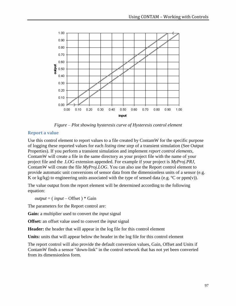
Using CONTAM – Working with Controls
97
Figure – Plot showing hysteresis curve of Hysteresis control element
Report a value
Use this control element to report values to a file created by ContamW for the specific purpose
of logging these reported values for each listing time step of a transient simulation (See Output
Properties). If you perform a transient simulation and implement report control elements,
ContamW will create a file in the same directory as your project file with the name of your
project file and the .LOG extension appended. For example if your project is MyProj.PRJ,
ContamW will create the file MyProj.LOG. You can also use the Report control element to
provide automatic unit conversions of sensor data from the dimensionless units of a sensor (e.g.
K or kg/kg) to engineering units associated with the type of sensed data (e.g. ºC or ppm(v)).
The value output from the report element will be determined according to the following
equation:
output = ( input – Offset ) * Gain
The parameters for the Report control are:
Gain: a multiplier used to convert the input signal
Offset: an offset value used to convert the input signal
Header: the header that will appear in the log file for this control element
Units: units that will appear below the header in the log file for this control element
The report control will also provide the default conversion values, Gain, Offset and Units if
ContamW finds a sensor "down-link" in the control network that has not yet been converted
from its dimensionless form.
Using CONTAM – Working with Controls
98
Signal split
Use this to split a signal, so the same signal can be directly linked to multiple nodes in the
control network.
Logical
Use these controls to provide logical operations including:
Binary – convert input signal to binary 0 or 1,
NOT – negate single input value and provide binary output 0 or 1,
AND – perform AND operation on two input values and provide binary output 0 or 1.
output = 1 IF (input1 > 0) AND (input2 > 0)
output = 0 otherwise
OR – perform OR operation on two input values and provide binary output 0 or 1.
output = 1 IF (input1 > 0) OR (input2 > 0)
output = 0 otherwise
XOR – perform XOR operation on two input values and provide binary output 0 or 1.
output = 1 IF (input1 > 0) AND (input2 <= 0)
output = 1 IF (input2 > 0) AND (input1 <= 0)
output = 0 otherwise
Mathematical
Use these controls to provide mathematical operations including:
Absolute value – provide absolute value of input signal
Add, Subtract, Multiply, and Divide – perform operation on two input signals and provide
result as output.
Note the order of operation is important for Subtract and Divide.
Subtract: output = input1 – input2
Divide: output = input1 / input2
Sum and Average – Sum or average multiple input signals and provide result as output
signal. Three signals can be directly input to using links drawn into the control node icon,
and more can be cascaded through the use of phantom nodes.
EXP(x) – raise e to the power of x.
LN(x) – calculate natural logarithm of x.
LOG10(x) – calculate log base 10 of x.
POW(x,y) – raise x to the power of y where x is input1 and y is input2.
SQRT(x) – calculate the square root of x.
Polynomial(x) – calculate polynomial of x based on user-defined polynomial coefficients.
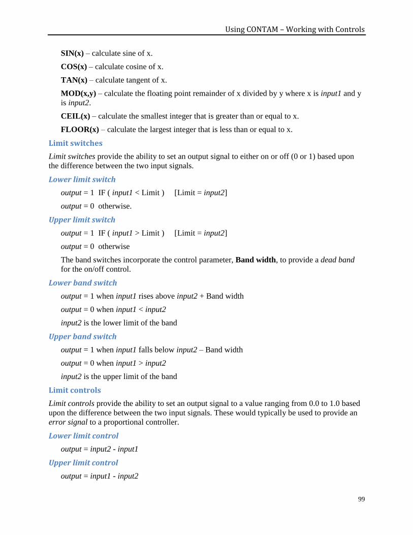
Using CONTAM – Working with Controls
99
SIN(x) – calculate sine of x.
COS(x) – calculate cosine of x.
TAN(x) – calculate tangent of x.
MOD(x,y) – calculate the floating point remainder of x divided by y where x is input1 and y
is input2.
CEIL(x) – calculate the smallest integer that is greater than or equal to x.
FLOOR(x) – calculate the largest integer that is less than or equal to x.
Limit switches
Limit switches provide the ability to set an output signal to either on or off (0 or 1) based upon
the difference between the two input signals.
Lower limit switch
output = 1 IF ( input1 < Limit ) [Limit = input2]
output = 0 otherwise.
Upper limit switch
output = 1 IF ( input1 > Limit ) [Limit = input2]
output = 0 otherwise
The band switches incorporate the control parameter, Band width, to provide a dead band
for the on/off control.
Lower band switch
output = 1 when input1 rises above input2 + Band width
output = 0 when input1 < input2
input2 is the lower limit of the band
Upper band switch
output = 1 when input1 falls below input2 – Band width
output = 0 when input1 > input2
input2 is the upper limit of the band
Limit controls
Limit controls provide the ability to set an output signal to a value ranging from 0.0 to 1.0 based
upon the difference between the two input signals. These would typically be used to provide an
error signal to a proportional controller.
Lower limit control
output = input2 - input1
Upper limit control
output = input1 - input2
Using CONTAM – Working with Controls
100
The upper and lower limit controls can be used to prepare an error signal for the proportional
controls. If the input signal to an upper limit control is greater than the limit value, a positive
output results; e.g., if a contaminant concentration is too high, the positive signal could activate
an airflow device. If the input signal to a lower limit control is lower than the limit value, a
positive output results; e.g., if the air flow through an opening is too low, a positive signal could
activate a fan to provide the required flow.
Proportional and Proportional–Integral
Proportional control
This is a model of a simple proportional controller where the input signal is an error signal that is
typically a sensed value minus a set-point value which is obtained by using other control
functions, e.g. the constant control. The input signal is multiplied by the proportionality constant
parameter of the control, Kp. The output signal is limited to values between 0 and 1, so you
should set the proportionality constant accordingly. The output signal could then be modified as
required using other control elements.
output = input Kp
Proportional-Integral control
This is a model of a simple P-I controller where the input signal is an error signal. The output
signal is limited to values between 0 and 1 and is modified by the control parameters Kp and Ki
according to the following equation.
output = output* + Kp (input - input*) + Ki (input + input*)
where output* and input* are the values of output and input at the previous time step. The Kp
and Ki factors must be tuned for the specific problem and time step. This is similar to an
"incremental" P-I algorithm described in equations (17-37) and (18-3) of [Stoecker and Stoecker
1989].
Scheduled Delay
This control element provides the ability to simulate time delays associated with the ramping
up/down of system components changing between states, e.g., the spin down of a fan or the
opening/closing of a damper. The scheduled delay element allows you to define a schedule
according to which the change of state occurs. The output will change according to this schedule
when the input changes.
Node Name: This is an optional name you can provide for this control node. This name can be
used to reference this node with a Phantom control node.
Schedule - Signal Increasing: Select/enter a day schedule that characterizes the delay in an
increasing signal. The schedule must be trapezoidal beginning with a value of 0.0 at time
00:00:00 and increase to a value of 1.0 before 24:00:00. Only one increasing time period per
schedule will be allowed.
Schedule - Signal Decreasing: Select/enter a day schedule that characterizes the delay in a
decreasing signal. The schedule must be trapezoidal beginning with a value of 1.0 at time
00:00:00 and decrease to a value of 0.0 before 24:00:00. Only one decreasing time period per
schedule will be allowed.
Using CONTAM – Working with Controls
101
Description: Enter an optional description for this control element.
Exponential Delay
This control element provides the ability to simulate time delays associated with the ramping
up/down of system components changing between states, e.g., the spin down of a fan or the
opening/closing of a damper. The exponential delay element allows you to define an exponential
delay based on a time constant.
Node Name: This is an optional name you can provide for this control node. This name can be
used to reference this node with a Phantom control node.
Time Constants:
Increase: Enter the amount of time it should take for the output signal to exponentially
increase by (1 – 1/e) % of the total change in the input signal when it rises from one state to
the next. The format is hh:mm:ss.
Decrease: Enter the amount of time it should take for the output signal to exponentially
decrease by (1 – 1/e) % of the total change in the input signal when it falls from one state to
the next. The format is hh:mm:ss.
NOTE: An amount of time of about 4.6 times the value entered above is required for the
output signal to increase/decrease by 99 % of the total change in the input signal.
Description: Enter an optional description for this control element.
Maximum and Minimum
The output will be the maximum or minimum of all input signals to the control node each time
step. Once a node is defined to be of this type, up to three input signals can be drawn directly
into it. More signals can be cascaded through the use of phantom control elements.
Node Name: This is an optional name you can provide for this control node. This name can be
used to reference this node with a Phantom control node.
Description: Enter an optional description for this control element.
Integrate over time
The output will be the integration over time of input signal 1 (horizontal) controlled by input
signal 2 (vertical). Integration occurs when input signal 2 > 0; there is no integration when input
signal 2 = 0; the integral is reinitialized to zero when input signal 2 < 0. A simple trapezoidal
integration method is used.
Running average
The output will be the average of the input signal integrated over the Time Span, tint:
out = ∫in dt / tint
At the start of simulation, when the simulated time is less than the time span, the output will be
the average of the input up to that time.
Node Name: This is an optional name you can provide for this control node. This name can be
used to reference this node with a Phantom control node.
Using CONTAM – Working with Controls
102
Time Span: Enter the amount of time included in the running average, tint. The format is
hh:mm:ss.
Description: Enter an optional description for this control element.
Continuous Value File and Discrete Value File (CVF/DVF)
These control elements allow you to implement general schedules by obtaining input values from
a file. This allows you to create schedules that are not restricted by the 12-day schedule limit of
CONTAM week schedules. These are text files that you create according to the format specified
in the CVF Format and DVF Format sections of this document. You can only use one of each
file per simulation, but the file may contain multiple lists of values. Value lists are referenced by
Value name, which are column headings in the files.
CVF and DVF files differ not only in format but also in behavior. During a simulation,
CONTAM will interpolate between the CVF values but not so for DVF values, i.e., they will
remain constant until a new value is encountered within the file.
Beginning with CONTAM version 3.2, these files can now be utilized without the use of an
associated control node/network, i.e., building components that may be associated with a
schedule can do so by directly associating them with a value name of a CVF/DVF file. This is
now apparent in the Schedule properties of each component within ContamW.
Value Name: Select the name of a set of values from the list of headings as they appear in the
CVF/DVF file.
File Name: This field displays the CVF/DVF file that contains the data that will be used by the
control node during simulation. You must use the DataControlsContinuous Values File…
and DataControlsDiscrete Values File… menu items to select the files you want to use
prior to creating the CVF/DVF control nodes.
Node Name: This is an optional name you can provide for this control node. This name can be
used to reference this node with a Phantom control node.
Continuous Values File (CVF) Format
You can use CVF files to implement schedules that are not limited to the twelve day types as are
CONTAM schedules. CVF values are made available to ContamX through the continuous values
file which has a .CVF file name extension. During simulation, ContamX will linearly interpolate
between the values provided in the CVF file. You create the text file according to the following
format using an external program.
The first line of the CVF is used to identify the type of file. It is exactly:
ContinuousValuesFile ContamW 2.1
The second line is a description of the file entered by the user:
desc[] // file description (I1) {W}; may be blank
The next line defines the period covered by the file:
StartDate // first date for DEF data (mm/dd IX)
EndDate // last date for DEF data (mm/dd IX)
The next section specifies the control node names:
_nbvfn // number of CVF node names
Using CONTAM – Working with Controls
103
followed by _nbvfn lines consisting of node names:
name[] // node name (I1)
The remainder of the file consists of data for all nodes for each date and time from StartDate to
EndDate:
date // date (mm/dd IX)
time // time of day (hh:mm:ss I4)
value[1] // value [?] for name[1] (R4)
...
value[_nbvf] // value [?]for name[_nbvf] (R4)
The node data must start at time 00:00:00 on the StartDate and end at 24:00:00 on the
EndDate. The times must be in consecutive order, but the difference between successive times
need not be constant.
The file description may not begin with a "!". The StartDate and EndDate are used to verify
that the file data covers the entire period to be simulated. The StartDate may not be later than
the EndDate. Data elements on a single line are separated by tabs. The data must be in time-
sequential order. The file values must be in the units needed for the signal created by the control
node.
Node names may not include imbedded blanks. Data for nodes that are not in the project file will
be ignored. If a CVF node name in the project file is not included in the CVF, a fatal error will
result. ContamW will assist the user by checking node names. ContamX will perform the name
check before simulation begins.
Discrete Values File (DVF) Format
You can use DVF files to implement schedules that are not limited to the twelve day types as are
CONTAM schedules. DVF values are made available to ContamX through the discrete values
file which has a DVF file name extension. As the name implies, ContamX will not interpolate
between the values provided in the DVF file. You create the text file according to the following
format using an external program.
The first line of the DVF is used to identify the type of file. It is exactly:
DiscreteValuesFile ContamW 2.1
The second line is a description of the file entered by the user:
desc[] // file description (I1) {W}; may be blank
The next line defines the period covered by the file:
StartDate // first date for DEF data (mm/dd IX)
EndDate // last date for DEF data (mm/dd IX)
The next section specifies the control node names:
_ndefn // number of DVF node names
followed by _ndefn lines consisting of:
name[] // node name (I1)
value // initial value [?] (R4)
Succeeding lines present data whenever a node value changes:
date // date (mm/dd IX)

Using CONTAM – Working with Controls
104
time // time of day (hh:mm:ss I4)
index // index into name[]
value // new value [?] (R4)
The file description may not begin with a "!". The StartDate and EndDate are used to verify
that the file data covers the entire period to be simulated. The StartDate may not be later than
the EndDate. Data elements on a single line are separated by tabs. The data must be in time-
sequential order. More than one node may change at the same time. The file values must be in
the units needed for the signal created by the control node.
Node names may not include imbedded blanks. Data for nodes that are not in the project file will
be ignored. If a DVF node name in the project file is not included in the DVF, a fatal error will
result. ContamW will assist the user by checking node names. ContamX will perform the name
check before simulation begins.
3.8.8 Control Super Elements
Prior to CONTAM version 2.2, ContamW required you to draw all control networks directly on
the main SketchPad even if they shared the same logic and control elements, leading to the
potential for much repetitive work. In order to minimize user input and to allow sharing of
control logic between different project files, controls have been enhanced to enable the creation
of Control Super Elements. Super Elements can be saved in the project file as well as in a new
CONTAM Library file type LB5.
Terminology Super Element - named control logic diagram and accompanying control elements (sub-nodes)
from the previously presented list of control elements. In object-oriented programming terms this
is similar to a class in that it is not actually used until it is instantiated as an object.
Super Node - an instantiated Super Element. In object-oriented programming terms this would
be an object or instance of a user-defined class.
Control Super Element / Super Node SketchPad With the advent of the new control super element, comes another use of the SketchPad to create
and edit super elements and super nodes. When working with super elements only the controls
drawing tool is enabled, along with the ability to define the control network icons. This
SketchPad is activated via the Data→Controls→Super Elements... menu item. When the Super
Element SketchPad is active, the upper left corner of the SketchPad will display "Super
Element:" followed by the name of the super element currently displayed on the SketchPad.
When working with super elements the "Control Super Elements" dialog box will also be
displayed as shown below.
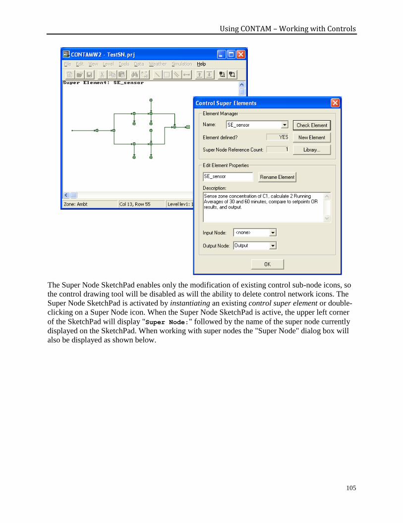
Using CONTAM – Working with Controls
105
The Super Node SketchPad enables only the modification of existing control sub-node icons, so
the control drawing tool will be disabled as will the ability to delete control network icons. The
Super Node SketchPad is activated by instantiating an existing control super element or double-
clicking on a Super Node icon. When the Super Node SketchPad is active, the upper left corner
of the SketchPad will display "Super Node:" followed by the name of the super node currently
displayed on the SketchPad. When working with super nodes the "Super Node" dialog box will
also be displayed as shown below.
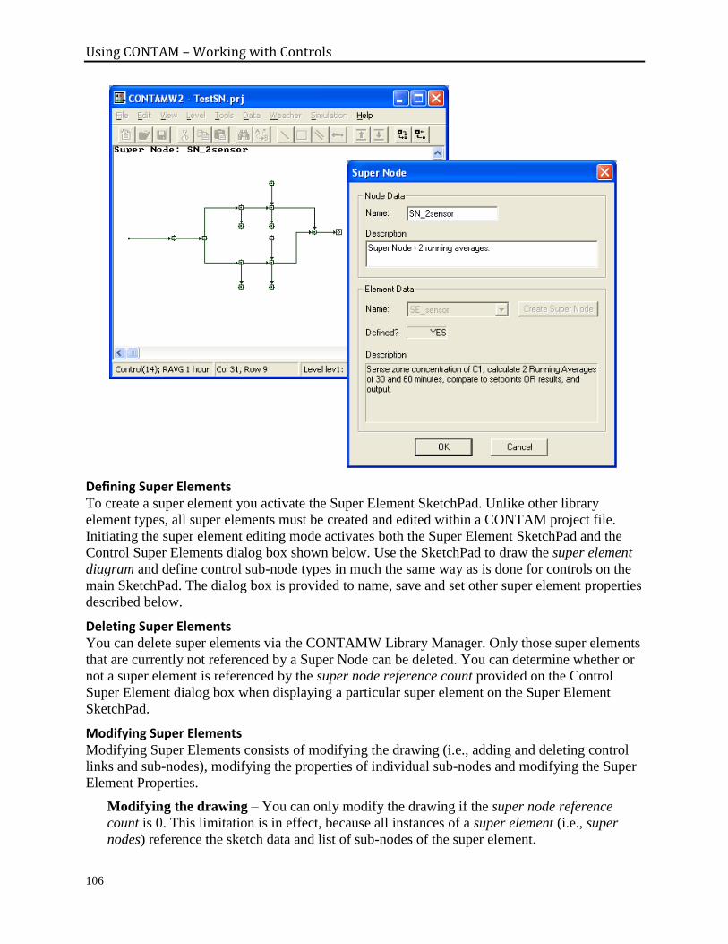
Using CONTAM – Working with Controls
106
Defining Super Elements To create a super element you activate the Super Element SketchPad. Unlike other library
element types, all super elements must be created and edited within a CONTAM project file.
Initiating the super element editing mode activates both the Super Element SketchPad and the
Control Super Elements dialog box shown below. Use the SketchPad to draw the super element
diagram and define control sub-node types in much the same way as is done for controls on the
main SketchPad. The dialog box is provided to name, save and set other super element properties
described below.
Deleting Super Elements You can delete super elements via the CONTAMW Library Manager. Only those super elements
that are currently not referenced by a Super Node can be deleted. You can determine whether or
not a super element is referenced by the super node reference count provided on the Control
Super Element dialog box when displaying a particular super element on the Super Element
SketchPad.
Modifying Super Elements Modifying Super Elements consists of modifying the drawing (i.e., adding and deleting control
links and sub-nodes), modifying the properties of individual sub-nodes and modifying the Super
Element Properties.
Modifying the drawing – You can only modify the drawing if the super node reference
count is 0. This limitation is in effect, because all instances of a super element (i.e., super
nodes) reference the sketch data and list of sub-nodes of the super element.
Using CONTAM – Working with Controls
107
Modifying sub-node properties – You can modify the properties of sub-nodes as you
desire. This will not affect existing instances of the super element; however, this will change
the default properties of new instances of the super element.
Modifying Super Element properties – You can modify the super element properties as
you so desire. This will not affect existing instances as super nodes simply reference the
super element properties, but do not create new instances of them.
Control Super Element Properties
This section provides information on utilizing the Control Super Element dialog box that
together with the Super Element SketchPad enables you to manage and define control super
elements and is activated via the DataControlsSuper Elements... menu item. There are
two section of information presented: Element Manager and Element Properties editor.
Element Manager This is used to select super elements for editing and creating new elements and activating the
CONTAMW Library Manager to work with Super Element Library files.
Name: This combo box provides you with the name of the currently active super element for
which the sketch data is also displayed on the Super Element SketchPad. The name should also
appear on the upper left corner of the sketchpad. You can also select other existing super
elements from the drop down list. This will change the super element displayed upon the
sketchpad as well as the properties displayed on this dialog box.
Check Element: While working with a super element, you can perform a check on it to
determine if is a fully defined super element. If the check passes then the super element is
considered to be fully defined. If the check fails, then ContamW will provide feedback in the
form of messages and highlighting of errors on the sketch. Even though a super element is
undefined, it can still be saved in its incomplete form.
There are a few basic reasons why the check could fail. Super elements are very similar to
control networks on the main SketchPad, so undefined super elements can result from problems
similar to main SketchPad control network as well as problems specific to super elements.
Potential reasons for undefined Super Elements:
Undefined sub-nodes (i.e., undefined sketch icons)
Incorrect number of inputs to control nodes
Circular control logic
No Output Node set
Pre-defined input to Input Node
New Element: This will create new super element having a default name of "SE_##" where ##
will depend on the number of existing super elements. New super elements have no sketch data,
so the SketchPad will be cleared. Once you create a super element, you do not have to save it.
Any modification you make to the sketch and properties will be maintained automatically with
the exception of the name which you must set via the "Rename Element" feature.
Using CONTAM – Working with Controls
108
Library: Use this feature to activate the CONTAMW Library Manager to create control library
files, copy super elements to and from super element library files (type LB5) and delete unused
super elements from the current project file. (See Working with Data and Libraries)
Element defined? This feature indicates whether or not a super element is fully defined (as
determined by ContamW) meaning it can be instantiated to create super nodes. Element
definition is verified by "checking." Checking is performed using the "Check Element" feature
described above, when you switch the currently displayed super element from the list of names,
or when you close the Control Super Elements dialog box, i.e., exit the super element editing
mode.
Super Node Reference Count: This is the number of instantiated super nodes that reference, the
super element. The super element can not be deleted from the project file unless this count is
equal to zero.
Edit Element Properties These are the user-defined properties of the super element other than the sketch and control
nodes. These properties include the Name, Description, Input Node name and Output Node
name.
Rename Element: Use this feature to enter a new name for the super element and change it with
the accompanying button. The new name will be compared to existing names before being reset.
Description: Provide a detailed description of the super element of up to 255 characters. This
description will be displayed in the CONTAMW Library Manager. The description and the super
element name are currently the only means by which to identify the super elements when
viewing them in the library manager.
Input Node: The input node of the super element is the sub-node which will receive an input
signal if one is drawn to an instantiated supernode on the main SketchPad. This is not required to
be set. If needed, select a sub-node to serve as the main input for the super element from the list
of named sub-nodes. Note that you must have provided a name for the sub-node which you wish
to make the input node, and the sub-node must be of a type that accepts at least one input.
Multiple inputs
If you require a super element with multiple inputs, you can define a sub-node to be of type
phantom. Once you instantiate a super node from the super element, you can select a named
control element that you want the phantom sub-node to reference.
Output Node: The output node of the super element is the sub-node from which the signal will
be provided to an output drawn from an instantiated super node on the main SketchPad. This is
required to be set for a super element to be defined. Note that when instantiated, the output node
will assume the name of the super node for the purposes of referencing with phantom nodes on
the main SketchPad.
Using CONTAM – Working with Controls
109
Control Super Nodes
Super nodes are instances of super elements having the same control logic and set of sub-nodes
as the super element. When you instantiate a super node from a super element, it takes on the
default values of the super element's sub-nodes; however, you can modify the values of the sub-
node parameters as needed.
Creating Super Nodes To create a super node, you select the Super element... from the Control Element Types dialog
box just as you would define any other control node on the main SketchPad (See Defining
Controls). This will activate the Super Node SketchPad mode and the accompanying Super Node
dialog box. You then work with both the dialog box and sketchpad to select a super element to
instantiate and to modify the sub-nodes as you require for the particular instance (See Control
Super Node Properties).
Once you have created the super node and exited the super node editing mode, the super node
will appear as a single icon (super node icon) on the main SketchPad.
Deleting Super Nodes You delete super nodes from the main SketchPad by simply highlighting the super node icon and
pressing the delete key on the keyboard or selecting EditDelete from the main menu. If any of
the sub-nodes of the deleted super node are referenced by phantom nodes, you will be informed
and prompted as to whether you want to undefine the phantom nodes (and sub-nodes) that
reference them.
Modifying Super Nodes Once you have instantiated a super node, you can modify the sub-nodes of a super node.
Activate the super node editing mode by double-clicking the super node icon on the main
SketchPad. Simply double-click on the sub-nodes whose properties you wish to modify and edit
them as you would nodes on the main SketchPad. Note that you can not modify the sketch in any
way, i.e., you can not draw or delete sub-nodes.
Control Super Node Properties
This section provides information on utilizing the Super Node dialog box that together with the
Super Node SketchPad enables you to manage and define control super nodes. This dialog box is
activated when creating a new super node or when modifying an existing one. There are two
section of information presented: Node Data and Element Data.
Node Data This displays super node specific data used to identify a specific super node.
Name: As with all control node types, you can provide a name for the super node. Named
super nodes can be referenced by phantom nodes. When you name a super node, its output
sub-node will also be given the same name, because the output sub-node will be the node
actually referenced by any phantom nodes that refer to the super node.
Description: Enter a detailed description of the super node to help you identify the super
node. This description will appear in the status bar when you highlight the super node icon
on the SketchPad.
Using CONTAM – Working with Controls
110
Element Data This section enables you to select and set the super element from which to instantiate a new
super node. Once instantiated this section simply provides information on the super element from
which the super node was instantiated.
Name: Prior to instantiation of a super node, this combo box provides you with the name of
the currently active super element for which the sketch data is also displayed on the Super
Element SketchPad. The name should also appear in the upper left corner of the SketchPad.
You can also select other existing super elements from the drop down list. This will change
the super element displayed upon the sketchpad as well as the properties displayed on this
dialog box.
Create Super Node: Click this button to instantiate a super node from the currently selected
super element. Once instantiated, this button will be disabled along with the Name drop
down combo box.
Note that when creating a new super node, until you create the super node, any changes you
make to sub-nodes of the displayed super element will modify sub-nodes of the super
element and not a super node.
Defined?: This indicates whether or not the currently selected super element is fully defined
– if "YES" then a super node can be instantiated from the super element, otherwise not.
Description: This displays the detailed description of the currently displayed super element.

Using CONTAM – Working with Species and Contaminants
111
3.9 WORKING WITH SPECIES AND CONTAMINANTS
Airborne contaminants are dispersed throughout buildings due to multiple transport mechanisms.
These include air movements into, out of, and within a building system; heating, ventilating, and
air-conditioning (HVAC) systems; removal by filtration, deposition, and sorption; generation and
resuspension; chemical reaction; and radio-chemical decay. CONTAM provides you with the
ability to simulate these methods of dispersal of airborne contaminants within built structures.
Species is a general term used (by CONTAM) to identify substances that can be used as
contaminants during a simulation, i.e., contaminants are those species you designate to be used in
a simulation. You can include as many species/contaminants as you need within a project.
CONTAM handles both trace and non-trace contaminants. Trace contaminants are those that
exist at concentrations that do not cause a "significant" change in the density of air. Non-trace
contaminants are those that can affect the density of the air. The mass fractions of non-trace
contaminants will always sum to 1 kg/kg, i.e., they are the constituents of the air.
In versions prior to CONTAM 2.4 an underlying assumption of the model was that each zone is
considered to have a single concentration value at any given time. This assumption is sometimes
referred to as the "well-mixed" zone assumption. With respect to contaminant analysis, this
means that there are no spatial concentration gradients within a given zone. However, beginning
with version 2.4, zones can be pre-configured by the user to be one-dimensional
convection/diffusion zones in which contaminants can vary along a user-defined axis and
simulated using the short time step method (see Run Control Properties and One-Dimensional
Convection-Diffusion FlowError! Reference source not found.). Beginning with CONTAM
version 3.0, a single region of a building/project can be considered as a computational fluid
dynamics (CFD) zone (Detailed Zone Properties). A CFD calculation is used to determine three-
dimensional pressure, airflow and contaminant concentration fields within the CFD zone.
You can use CONTAM to perform steady state, transient, and cyclical contaminant analysis.
Steady state analysis refers to the determination of contaminant concentrations under steady flow
conditions. Transient analysis refers to the determination of the time history of contaminant
concentrations within each zone for a set of discrete time-steps. With a transient analysis you can
implement the effects of varying ambient contaminants using a contaminant file (See
Contaminant Files). A cyclic analysis determines the time history of contaminant concentrations
for a 24 h period such that the concentrations at the beginning and end of the 24 h period are the
same for each zone.
With CONTAM you must define contaminants in order to utilize the features that CONTAM
provides to simulate the generation of contaminants by sources, the removal by sinks (including
filters and kinetic reactions), and to determine occupant exposures. Contaminants must be
created/defined prior to implementing any of these contaminant-dependent features of
CONTAM. Prior to implementing contaminants within a project, you can first define the
building layout on the SketchPad, define all airflow paths (including ducts) and test your
building model by performing a steady state airflow simulation.
3.9.1 Non-trace Contaminants and Water Vapor
CONTAM handles non-trace contaminants, which are those contaminants that you define to be
the constituents of air. Typically, you might want to treat water vapor as a non-trace
contaminant. CONTAM will treat a contaminant with the name "H20" as water vapor. The
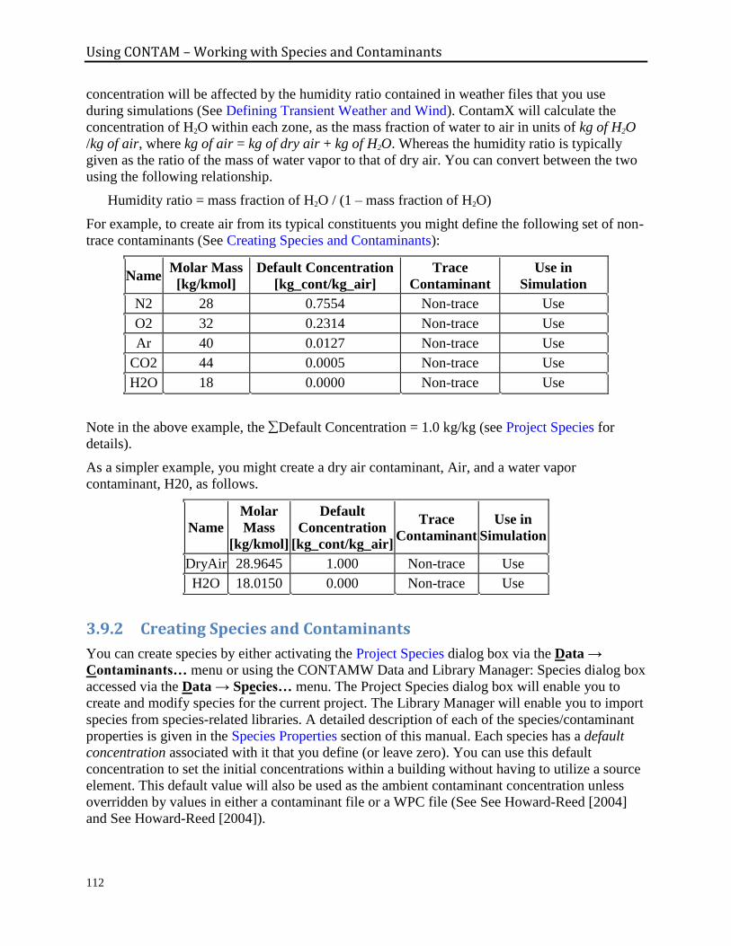
Using CONTAM – Working with Species and Contaminants
112
concentration will be affected by the humidity ratio contained in weather files that you use
during simulations (See Defining Transient Weather and Wind). ContamX will calculate the
concentration of H2O within each zone, as the mass fraction of water to air in units of kg of H2O
/kg of air, where kg of air = kg of dry air + kg of H2O. Whereas the humidity ratio is typically
given as the ratio of the mass of water vapor to that of dry air. You can convert between the two
using the following relationship.
Humidity ratio = mass fraction of H2O / (1 – mass fraction of H2O)
For example, to create air from its typical constituents you might define the following set of non-
trace contaminants (See Creating Species and Contaminants):
Name Molar Mass
[kg/kmol]
Default Concentration
[kg_cont/kg_air]
Trace
Contaminant
Use in
Simulation
N2 28 0.7554 Non-trace Use
O2 32 0.2314 Non-trace Use
Ar 40 0.0127 Non-trace Use
CO2 44 0.0005 Non-trace Use
H2O 18 0.0000 Non-trace Use
Note in the above example, the Default Concentration = 1.0 kg/kg (see Project Species for
details).
As a simpler example, you might create a dry air contaminant, Air, and a water vapor
contaminant, H20, as follows.
Name
Molar
Mass
[kg/kmol]
Default
Concentration
[kg_cont/kg_air]
Trace
Contaminant
Use in
Simulation
DryAir 28.9645 1.000 Non-trace Use
H2O 18.0150 0.000 Non-trace Use
3.9.2 Creating Species and Contaminants
You can create species by either activating the Project Species dialog box via the Data →
Contaminants… menu or using the CONTAMW Data and Library Manager: Species dialog box
accessed via the Data → Species… menu. The Project Species dialog box will enable you to
create and modify species for the current project. The Library Manager will enable you to import
species from species-related libraries. A detailed description of each of the species/contaminant
properties is given in the Species Properties section of this manual. Each species has a default
concentration associated with it that you define (or leave zero). You can use this default
concentration to set the initial concentrations within a building without having to utilize a source
element. This default value will also be used as the ambient contaminant concentration unless
overridden by values in either a contaminant file or a WPC file (See See Howard-Reed [2004]
and See Howard-Reed [2004]).
Using CONTAM – Working with Species and Contaminants
113
3.9.3 Deleting Species and Contaminants
You can delete species using the Delete button of the Project Species dialog box or of the
CONTAMW Data and Library Manager: Species dialog box. Species can not be deleted if they
are associated with a source/sink, filter or kinetic reaction. For those species for which an
association exists, the Delete buttons will be deactivated. You can also disable the use of a
contaminant within a simulation by deselecting the "Use in Simulation" box for a given species
from within the Species Properties dialog box.
3.9.4 Modifying Species and Contaminants
Once you have created species for a project, you can modify any of the related parameters. This
is done by using the Edit button from within the Species Properties dialog box that is accessed
via the Data → Contaminants… menu item. ContamW will allow you to change the name of an
existing contaminant without affecting any of the currently associated sources, sinks, filters or
kinetic reactions as they reference contaminants by an internal index created by ContamW.
3.9.5 Project Species
Species must be defined before any related elements (e.g. source/sinks, filters and kinetic
reactions) can be defined. From the Project Species page any previously defined species may be
viewed, edited, or deleted and new species may be defined. The following describes the
information that appears on the Project Species dialog box.
Species: This is a list of the species that are currently defined within the current project.
Species Properties: These are the properties of the currently highlighted species.
Contaminants: This is a list of the project species for which the "Use in Simulation" property is
set to "Use," i.e., these are selected to be contaminants in the simulation.
Contaminant Summary: This is a summary of contaminant-related information including the
number of non-trace contaminants and the summation of the default concentrations of the non-
trace contaminants which must be 1.0.
NOTE: If the project contains water vapor, H2O, then its default concentration is not included
in this summation at this point, however, it will be accounted for by ContamX during simulation
if initial concentrations are set to ambient (see Simulation - Airflow Numerics Properties).
New, Edit and Delete: Click the "New" button to create a new species, or use the "Library..."
button to import/export species from/to a species library file. To modify the properties of an
existing species, highlight the species in the species list and click the "Edit" button. Click the
"Delete" button to delete the selected species.
IMPORTANT: Changing the number of contaminants, i.e. those species used in the simulation,
will reset the initial concentrations of all zones to the default contaminant concentrations. You
can reset all of these concentrations via the Run Control Properties of the simulation parameters
or via the Contaminant Data properties of the individual zones.
Using CONTAM – Working with Species and Contaminants
114
3.9.6 Species Properties
This section provides detailed descriptions of the specific species properties.
Name: You will use this name to refer to the species throughout the program. You must give
each species a name that is unique to the current project.
Molar Mass: The molar mass in g/mol or kg/kmol. CONTAM uses this value to convert
volumetric concentrations to mass fractions and to calculate the gas constant of the air mixture
made up by non-trace contaminants. You must enter a value of at least 1.0.
Default Concentration: CONTAM will apply this value as the default initial concentration for
each zone that you create. You can revise the initial concentration for individual zones as per
your requirements. This is also the ambient contaminant concentration during simulations which
do not utilize contaminant data from one of the external contaminant data files (CTM or WPC).
Diffusion Coefficient: This value will be used during simulations using the 1D Duct Model of
the Short Time Step Method (See Run Control Properties in the Working with Simulations
section). The dispersal coefficient will be calculated from this value depending on the Reynolds
Number in a given duct segment.
Mean Diameter: Enter the mean particle diameter if this species is to be a particulate type
species. CONTAM utilizes this value when converting between particle count units and particle
mass and volume units and to determine filter efficiency of Simple Particle Filter elements for
this size particle (See Simple Particle Filter in the Working with Filters section).
NOTE: This is not necessarily meant to be, for example, the aerodynamic diameter as the current
contaminant source models do not treat particles different from gaseous contaminants.
Effective Density: Enter a density that you want CONTAM to use as the effective density of a
species you want to consider to be a particulate type species. Currently, CONTAM only utilizes
this value when converting between particle count units and particle mass and volume units.
Specific Heat: The specific heat of a contaminant will used during simulation only when the
Variable Junction Temperatures method is selected.
Decay Rate: This is an exponential decay constant based upon the half-life of the radioactive
species calculated using the following equation:
Decay Rate = ln(2) / 1/2,
where 1/2 is the half-life of the radioactive species in seconds.
ContamW will use this value to perform unit conversions for radioactive contaminants.
Radioactive species are only distinguished from other species by the units associated with them,
not by modeling the radioactive decay process. To model a radioactive decay, use a kinetic
reaction (See Kinetic Reaction Data).
UVGI Susceptibility Constant: A species-dependent rate constant used to determine
UVGI filter effectiveness for a specific contaminant [m2/J]. Values for several species are
provided in [Kowalski, et al. 2000] and they range from 10-3 cm2/J to 10-6 cm2/J. (new for
version 3.2)
Using CONTAM – Working with Species and Contaminants
115
Non-Trace Contaminant: Non-trace contaminants are those that can affect the density of the
air, i.e., are considered components of the air. (See Non-trace Contaminants and Water Vapor)
Use in Simulation: This determines whether or not a species will be a contaminant. Checking
"Use in Simulation" indicates that a species will be a contaminant and used in the simulation.
Description: Use this to provide a more detailed description of the species.
Guideline Value: Currently not implemented.
Guideline Description: Currently not implemented.
3.9.7 Contaminant Files
You can account for changes in the ambient contaminant concentrations when performing
transient contaminant simulations using ambient contaminant (CTM) files. If you associate a
contaminant file with your project (see Run Control Properties) ContamX will compare those
contaminants defined within your project file with those contained in the contaminant file. If
they match, ContamX will use the ambient concentrations in the contaminant file within the
simulation, otherwise they will be ignored.
You create the contaminant files external to ContamW. You can use a utility program provided
by NIST, Weather 2.0, to convert existing CONTAM 1.0 weather (which previously contained
ambient contaminant concentrations) files to CONTAM 2.0 weather and contaminant files.
Note that with this method the ambient concentration does not vary spacially, only temporally. If
you require spacial variations of outdoor contaminant level, then refer to the section entitled
Working with WPC Files.
Contaminant (CTM) File Format The CONTAM contaminant (species) file is a tab-delimited ASCII text file. These files are
easily created, imported and modified using common spreadsheet applications. They can be
saved as tab-delimited text files for use with CONTAM. In the listing below I1 indicates a
character string, I2 indicates a short integer and R4 indicates a four-byte real number. Individual
lines of data are separated by dashes (these dashes are only shown here for format presentation
purposes and should not be included in the actual files). Each day must begin with time 00:00:00
and end with time 24:00:00. The time interval between 00:00:00 and 24:00:00 can be either
regular or irregular – ContamX will interpolate as necessary. Comments are allowed and are
indicated by an "!" (exclamation point). Anything that appears on a line following a comment
indicator is ignored by the contaminant file reader.
SpeciesFile ContamW 2.0 ! file and version identification
-----
I1 Descr[] ! species file description
-----
I1 StartDate ! day of year (1/1 – 12/31)
I1 EndDate ! day of year (1/1 – 12/31)
I2 NumCont ! number of species
-----
I1 Name[1] ! name of species 1 (16 characters max)
I1 Name[2] ! name of species 2

Using CONTAM – Working with Species and Contaminants
116
...
I2 Name[NumCont] ! name of species NumCont
-----
!Date Time Name[1] Name[2] ... Name[NumCont]
-----
! for each day: start_date – end_date
! for each time: 00:00:00 - 24:00:00 increment may be variable
I1 Date ! date (1/1 – 12/31)
I1 Time ! time of day 00:00:00 – 24:00:00
R4 Conc[1] ! concentration of species 1
R4 Conc[2] ! concentration of species 2
...
R4 Conc[NumCont] ! concentration of species nc
! [kg_species/kg_air]
-----
Editing Contaminant Files You can import ambient files into a spreadsheet program for editing. However you must make
sure that the date format is compatible with CONTAM when you save the file. One well-known
spreadsheet program will convert the CONTAM date format of mm/dd into the mmm-dd form.
For example the CONTAM date format for January 1 is "1/1", but the spreadsheet program will
convert it to "Jan-01" unless you "force" it to import the first column of data – the one that
contains date information – as text. Another option is to accept the default importing option then
change the cell format for each date to the CONTAM format mm/dd prior to saving the file as
tab-delimitted.
Contaminant Unit Conversions Gaseous contaminants – to convert from ppm to:
kg/kg = (ppm MW) / (1 000 000 Vs air)
mg/L = (ppm MW) / (1 000 Vs)
mg/m3 = (ppm MW) / Vs
mg/ft3 = (ppm MW) / (35.3147 Vs)
Particle Contaminants – to convert from #/m3 to kg/kg:
where:
MW = molar mass of contaminant [kg/kmol]
Vs = 24.05 m3 which is the volume of one kmol of air at T = 20 ºC and P = 101 325 Pa (1
atm)
air = 1.204 kg/m3 at T = 20 ºC
eff = effective particle density [kg/m3]
Dmean = mean particle diameter [m]
Using CONTAM – Working with Sources and Sinks
117
3.10 WORKING WITH SOURCES AND SINKS
Sources and sinks are used to generate contaminants within and remove contaminants from
zones. Sources can be used to simulate building materials such as carpet, pieces of furniture, and
episodic events such as the use of cleaning products. You can define an almost unlimited number
of sources within a project.
To implement a source/sink, you must first define the species with which you want the
source/sink to be associated. You then place a source/sink icon within a zone on the SketchPad.
Once you place source/sinks on the SketchPad, you can define their characteristics, move, copy,
and delete them. You must associate each source/sink with a predefined species and provide
specific information that describes its emission and/or removal characteristics.
NOTE: It is important to note that even though you associate a species with each source/sink,
only those species that are designated to be contaminants will actually be used when performing
simulations (See Species Properties).
Much of the information that describes the characteristics of a source/sink is contained in
source/sink elements that you must create when defining source/sinks. The details of drawing,
defining and modifying sources and sinks are described in the following sections.
3.10.1 Source/Sink Elements
CONTAM uses mathematical relationships referred to as source/sink elements or models to
implement sources and sinks when performing contaminant simulations. CONTAM can
implement several source/sink models to generate contaminants within or remove contaminants
from a zone. Depending on the source/sink model, it could be used to emulate either a source, a
sink or both. Each of these source/sink element types is described in detail in the Source/Sink
Element Types section. Every source/sink must refer to a single source/sink element; however,
multiple source/sinks can refer to the same source/sink element.
Source/sink elements can also be stored within a CONTAM library file and shared between
different CONTAM project files (See Working with Data and Libraries).
3.10.2 Creating Sources and Sinks
You create source/sinks by placing a source/sink icon on the SketchPad (See Drawing Building
Component Icons). You must first define at least one species before ContamW will allow you to
place a source/sink icon upon the SketchPad. Each source/sink must be placed within a building
zone. You cannot place them in the ambient zone. Ambient sources are handled using either the
initial concentration property of a contaminant (for steady state simulations) or the concentration
contained within a weather file (for transient simulations). The "Source/sink" menu selection will
be disabled (grayed out) if you pop-up on a location where ContamW does not allow the icon to
be placed.
3.10.3 Deleting Sources and Sinks
You delete source/sink icons using the icon deletion procedure (See Deleting Building
Component Icons). Deleting source/sink icons from the SketchPad does not delete any
source/sink elements that you may have defined. These elements can only be deleted using the
CONTAMW Library Manager, accessible through the Data → Source/Sinks... menu.
Using CONTAM – Working with Sources and Sinks
118
3.10.4 Modifying Sources and Sinks
To modify the parameters of a source/sink, you use the icon definition procedure (See Defining
Building Component Icons) to display its properties and make the desired changes. You can also
move and copy source/sinks.
Moving Source/Sink Icons Once you define a source/sink, you can move the icon using the Cut and Paste functions of the
Edit menu. You can move the source/sink icon anywhere within the zone in which it is currently
located.
Copying Source/Sink Icons Once you define a source/sink, you can copy the icon using the Copy and Paste functions of the
Edit menu. You can copy a source/sink to any blank cell within a zone on any level of a project.
3.10.5 Defining Sources and Sinks
After you draw a Source/Sink icon on the SketchPad you must define it using the icon definition
procedure (See Defining Building Component Icons) to display and edit the properties. This will
display the "Source/Sink Properties" property sheet. Detailed descriptions of all source/sink
properties are given in the Source and Sink Properties section of this manual. Once you have
defined the properties, the icon will be displayed in black. From now on, you use this icon to
access the properties of the source/sink.
Among the properties associated with a source/sink are optional multiplier and schedule
information. You would use the multiplier to proportionally increase the generation or removal
of a contaminant for a particular source/sink. For example, if you have created a source/sink
element with a certain emission rate per square meter of surface area (such as a floor covering),
you could use this multiplier to account for the surface area of the source/sink for each zone in
which you place a source/sink implementing this source/sink element. You could use a schedule
to vary the emission/removal characteristics of a source/sink with time. For example, you could
provide a schedule for an episodic source (burst source) that would periodically cause the release
of a contaminant when performing a transient simulation.
3.10.6 Source and Sink Properties
This section provides detailed descriptions of the specific source/sink properties. Each of the
following subsections are the context-sensitive help topics that you can access by pressing F1
when working with property pages of the "Source/Sink Properties" property sheet.
Source/Sink - Source/Sink Element Properties
Source/Sink Number: This is the number that appears in the status bar when you highlight an
icon. ContamW automatically assigns this number to each source/sink once they are defined.
This number could change as you add and remove source/sinks to or from a project. Each time
you save a project, the source/sink numbers are reassigned. Numbers are assigned beginning on
the top level, starting from the upper-left corner of the SketchPad, moving left-to-right and top-
to-bottom of the SketchPad.
Source/Sink Element: The source/sink element provides the mathematical model to be
associated with the selected source/sink.
Description: Displays the description property of the element selected in the "Name" field.
Using CONTAM – Working with Sources and Sinks
119
Name: <required> Select a source/sink element from those contained in the Name list. You
can add elements to the list by creating new elements within the project or importing them
from a library file. Use the "New Element" button to define a new element. Activate the
CONTAMW Library Manager to import elements from library files via the “Library” button
(See Working with Data and Libraries). Use the "Edit Element" button to modify the
properties of the element displayed in the Name field.
Model Summary: This summarizes the information associated with the source/sink element
whose name is currently displayed in the Name field.
Source/Sink - Multiplier and Location Properties
Source/Sink Number: This is the number that appears in the status bar when you highlight an
icon.
This is the number that appears in the status bar when you highlight an icon.
Source/Sink Number: This is the number that appears in the status bar when you highlight an
icon.
Multiplier: A constant value by which the source strength will be multiplied during simulation.
With this feature you could define a source/sink element having a source strength per unit area
then use the multiplier as the area of the zone for each source/sink that uses the per unit area
source/sink element.
NOTE: The multiplier serves as the surface area for the Boundary Layer Diffusion Model, and
should be entered in units of m2.
Initial Concentration: Some source/sinks are reversible in that they enable storage within or on
the surface and re-emission or resuspension of contaminant from the surface. These source/sinks
actually contribute a contaminant node to the contaminant transport equations. Currently, there
are two such element types: Boundary Layer Diffusion Controlled and Deposition with
Resuspension. The Initial Concentration properties will be enabled for these element types, and
you can set the values and units of these initial loadings.
Location: These are the X, Y and Relative Elevation (Z) coordinates and units for the selected
source/sink. X and Y are absolute coordinates and Rel Elevation is relative to the level on which
the source/sink is located. To create a point source, set the Minimum and Maximum values to be
the same. To create a source which distributes emissions along the 1D axis of the zone, enter
Minimum and Maximum values that span the desired region of the zone in which the source is
located.
These values are required for any source/sink that is located within a 1D convection/diffusion
zone (see 1D Zone Data). These coordinates will be verified by ContamW against the axis of the
1D zone in which it is located. This verification will be performed automatically when you select
either the Run Simulation or Create a ContamX Input File command from the Simulation
menu.
CFD Source ID: Each source/sink that is located within a CFD zone must be given a unique
identifier. This id will be used to identify the source/sink within the CFD0 Editor that is used to
define the location of the interface paths with respect to the CFD zone.
Using CONTAM – Working with Sources and Sinks
120
Source/Sink - Schedule Properties
Source/Sink Number: This is the number that appears in the status bar when you highlight an
icon.
Schedule: You can use a schedule to modify the source strength as a function of time. Two
source/sink element types, Burst Source and Decaying Source, require the use of a schedule. If
there are previously defined schedules within the current project, you may select one from the
Name list. Click the "New Schedule" button to define a new schedule. To view or modify an
existing schedule click the "Edit Schedule" button. Setting this field to <none> indicates no
schedule (See See Howard-Reed [2004]).
CVF/DVF Control: Values from either a CVF or DVF file can be used in place of the above
Schedule (read about CVF and DVF controls in the Control Element Types section). This
enables using these control element types without having to draw/define an associated control
network. The associated radio buttons "Use Neither", "Use CVF" and "Use DVF" are used to
select the desired control method. Select the heading name from the associated "Name" drop
down box that will display the headings of either the CVF or DVF file as per the aforementioned
radio button selection.
Control Status: This will display the current method of control: Schedule, direct CVF, direct
DVF or Control Network. If an actuator of a control network on the SketchPad is associated with
the scheduled item then it will take precedence over the Schedule and CVF/DVF Control. If
either the "Use CVF" or "Use DVF" radio button is selected then CVF or DVF will take
precedence over an associated schedule.
Source/Sink Element Types
These are the source/sink element types or models that you can implement with CONTAM.
Refer to the related information for each specific model to obtain detailed descriptions of them.
For the so-called surface elements, a surface results file can be generated that will provide the
transient loadings for each of these surface types (see Results Files in Working with Results).
CONTAM Elements Constant Coefficient Model: The general source/sink model allows constant contaminant
generation and deposition rates.
Pressure Driven Model: This model is for contaminant sources that are governed by the
pressure differences between zones.
Cutoff Concentration Model: This model will reduce emissions as the concentration within
the zone in which it is implemented approaches a specified cutoff concentration. This model
may be appropriate for some sources of Volatile Organic Compound (VOC).
Decaying Source Model: This model provides a source that will exponentially decay with
time according to a user-defined time constant. This model may also be appropriate for some
VOC sources.
Boundary Layer Diffusion Model: Used to model reversible diffusion of a contaminant
through the air-phase boundary layer of a material surface and the sorption of the
contaminant into a sink with a linear sorption isotherm.
Using CONTAM – Working with Sources and Sinks
121
Burst Source Model: Used to model an instantaneous release of a mass of contaminant
within a zone.
Deposition Velocity Sink Model: Used to model contaminant deposition onto a surface as
specified by a deposition velocity.
Deposition Rate Sink Model: Used to model contaminant deposition onto a surface as
specified by a deposition rate.
Deposition with Resuspension Model: Used to model contaminant deposition and
resuspension to and from a surface.
Super Source/Sink Element: The super element allows multiple elements of the other types
to be combined into a single element. This can reduce repetitious work required to create
multiple sources throughout a building by allowing multiple sources to be represented by a
single icon on the SketchPad.
NRCC Elements These sources are provided for compatibility with the Material Emissions Database developed by
the National Research Council Canada (NRCC) that is largely based on material emission test
chamber data [Howard-Reed 2004 and 2006].
Power Law Model: Constant emission rate until specified time after which time the
emission rate decays according to the power law relationship.
Peak Model: Constant emission rate until specified time at which the peak emission rate is
obtained after which time the emission rate decays according to the peak model relationship.
Source/Sink Element: Constant Coefficient Model
This is a generic source/sink element that provides for direct input of a contaminant generation
and removal rate. Units are provided in default calculation units.
S(t) = mult·ctrl·G - mult·ctrl·R C(t)
G = Generation rate [kg/s]
R = Effective removal rate [kgair/s]
Determine by multiplying the first-order removal rate of the contaminant [1/s] by air
density [kgair/m3] and volume [m3] of the zone in which the source is to be located.
C(t) = Concentration of contaminant in the zone [kg/kgair]
mult = Source/sink multiplier [no units]
ctrl = Schedule or control value [no units]
Name: Enter a unique name you want to use to identify the source/sink element. The element
will be saved within the current project and can be associated with multiple source/sinks.
Generation Rate: The rate at which the contaminant is introduced into the zone.
Removal Rate: The rate at which the contaminant is removed from the zone.
Species: Select a previously defined species from the drop down box.
Description: Field for entering a more detailed description of the specific sink/source element.
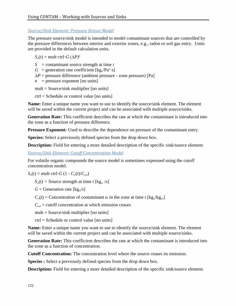
Using CONTAM – Working with Sources and Sinks
122
Source/Sink Element: Pressure Driven Model
The pressure source/sink model is intended to model contaminant sources that are controlled by
the pressure differences between interior and exterior zones, e.g., radon or soil gas entry. Units
are provided in the default calculation units.
S(t) = mult·ctrl·G P)n
S = contaminant source strength at time t
G = generation rate coefficient [kg/Pan·s]
P = pressure difference (ambient pressure - zone pressure) [Pa]
n = pressure exponent [no units]
mult = Source/sink multiplier [no units]
ctrl = Schedule or control value [no units]
Name: Enter a unique name you want to use to identify the source/sink element. The element
will be saved within the current project and can be associated with multiple source/sinks.
Generation Rate: This coefficient describes the rate at which the contaminant is introduced into
the zone as a function of pressure difference.
Pressure Exponent: Used to describe the dependence on pressure of the contaminant entry.
Species: Select a previously defined species from the drop down box.
Description: Field for entering a more detailed description of the specific sink/source element.
Source/Sink Element: Cutoff Concentration Model
For volatile organic compounds the source model is sometimes expressed using the cutoff
concentration model.
S(t) = mult·ctrl·G (1 - C(t)/Ccut)
S(t) = Source strength at time t [kg/s]
G = Generation rate [kg/s]
C(t) = Concentration of contaminant in the zone at time t [kg/kgair]
Ccut = cutoff concentration at which emission ceases
mult = Source/sink multiplier [no units]
ctrl = Schedule or control value [no units]
Name: Enter a unique name you want to use to identify the source/sink element. The element
will be saved within the current project and can be associated with multiple source/sinks.
Generation Rate: This coefficient describes the rate at which the contaminant is introduced into
the zone as a function of concentration.
Cutoff Concentration: The concentration level where the source ceases its emission.
Species : Select a previously defined species from the drop down box.
Description: Field for entering a more detailed description of the specific sink/source element.
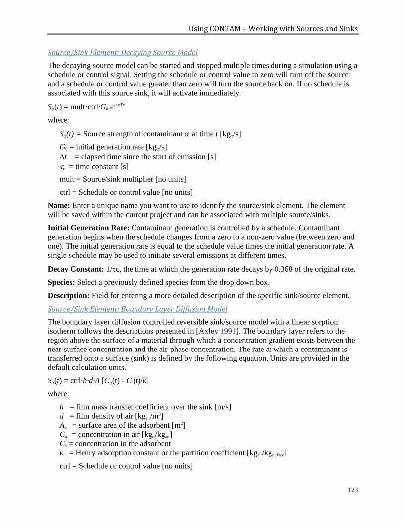
Using CONTAM – Working with Sources and Sinks
123
Source/Sink Element: Decaying Source Model
The decaying source model can be started and stopped multiple times during a simulation using a
schedule or control signal. Setting the schedule or control value to zero will turn off the source
and a schedule or control value greater than zero will turn the source back on. If no schedule is
associated with this source sink, it will activate immediately.
S(t) = mult·ctrl·G0 e-t/c
where:
S(t) = Source strength of contaminant at time t [kg/s]
G0 = initial generation rate [kg/s]
t = elapsed time since the start of emission [s]
c = time constant [s]
mult = Source/sink multiplier [no units]
ctrl = Schedule or control value [no units]
Name: Enter a unique name you want to use to identify the source/sink element. The element
will be saved within the current project and can be associated with multiple source/sinks.
Initial Generation Rate: Contaminant generation is controlled by a schedule. Contaminant
generation begins when the schedule changes from a zero to a non-zero value (between zero and
one). The initial generation rate is equal to the schedule value times the initial generation rate. A
single schedule may be used to initiate several emissions at different times.
Decay Constant: 1/c, the time at which the generation rate decays by 0.368 of the original rate.
Species: Select a previously defined species from the drop down box.
Description: Field for entering a more detailed description of the specific sink/source element.
Source/Sink Element: Boundary Layer Diffusion Model
The boundary layer diffusion controlled reversible sink/source model with a linear sorption
isotherm follows the descriptions presented in [Axley 1991]. The boundary layer refers to the
region above the surface of a material through which a concentration gradient exists between the
near-surface concentration and the air-phase concentration. The rate at which a contaminant is
transferred onto a surface (sink) is defined by the following equation. Units are provided in the
default calculation units.
S(t) = ctrl·h·d·As[C(t) - Cs(t)/k]
where:
h = film mass transfer coefficient over the sink [m/s]
d = film density of air [kgair/m3]
As = surface area of the adsorbent [m2]
C = concentration in air [kg/kgair]
Cs = concentration in the adsorbent
k = Henry adsorption constant or the partition coefficient [kgair/kgsurface]
ctrl = Schedule or control value [no units]
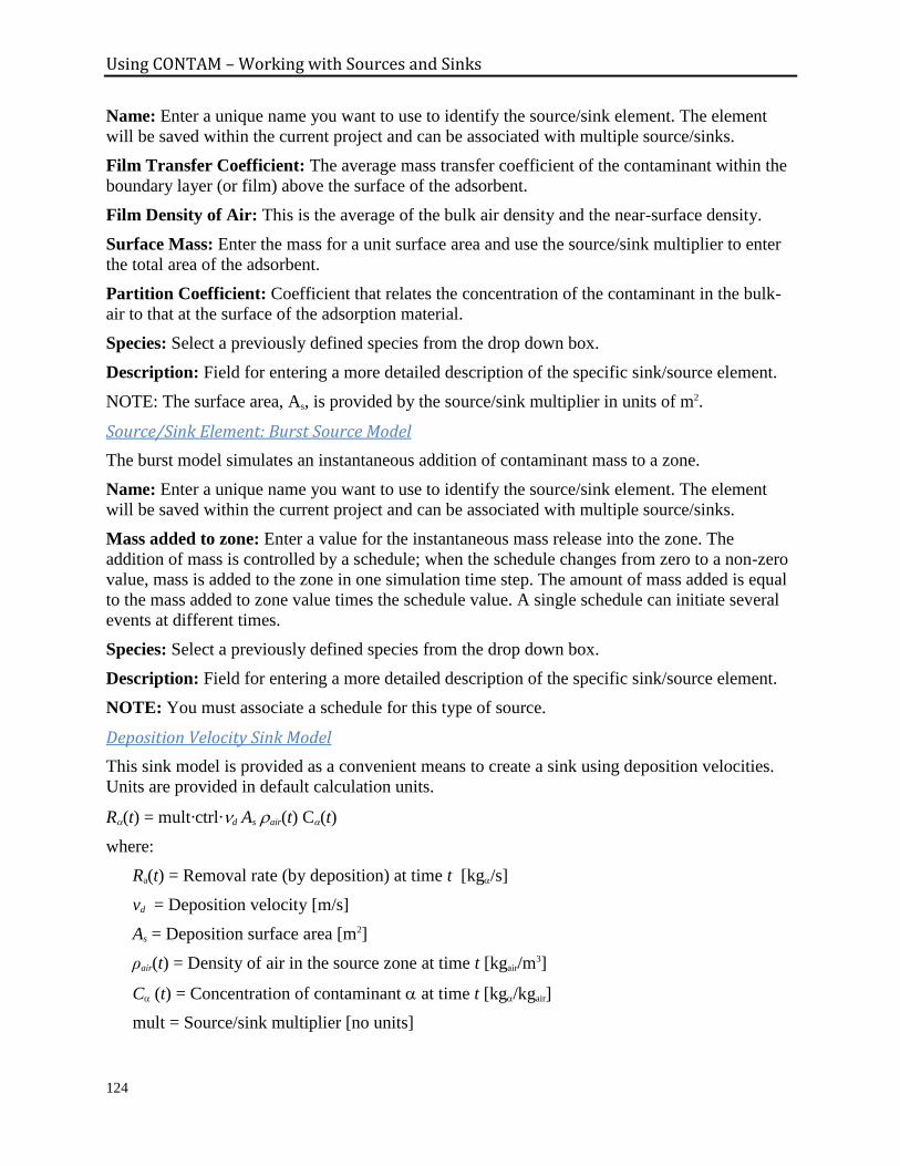
Using CONTAM – Working with Sources and Sinks
124
Name: Enter a unique name you want to use to identify the source/sink element. The element
will be saved within the current project and can be associated with multiple source/sinks.
Film Transfer Coefficient: The average mass transfer coefficient of the contaminant within the
boundary layer (or film) above the surface of the adsorbent.
Film Density of Air: This is the average of the bulk air density and the near-surface density.
Surface Mass: Enter the mass for a unit surface area and use the source/sink multiplier to enter
the total area of the adsorbent.
Partition Coefficient: Coefficient that relates the concentration of the contaminant in the bulk-
air to that at the surface of the adsorption material.
Species: Select a previously defined species from the drop down box.
Description: Field for entering a more detailed description of the specific sink/source element.
NOTE: The surface area, As, is provided by the source/sink multiplier in units of m2.
Source/Sink Element: Burst Source Model
The burst model simulates an instantaneous addition of contaminant mass to a zone.
Name: Enter a unique name you want to use to identify the source/sink element. The element
will be saved within the current project and can be associated with multiple source/sinks.
Mass added to zone: Enter a value for the instantaneous mass release into the zone. The
addition of mass is controlled by a schedule; when the schedule changes from zero to a non-zero
value, mass is added to the zone in one simulation time step. The amount of mass added is equal
to the mass added to zone value times the schedule value. A single schedule can initiate several
events at different times.
Species: Select a previously defined species from the drop down box.
Description: Field for entering a more detailed description of the specific sink/source element.
NOTE: You must associate a schedule for this type of source.
Deposition Velocity Sink Model
This sink model is provided as a convenient means to create a sink using deposition velocities.
Units are provided in default calculation units.
R(t) = mult·ctrl·d As air(t) C(t)
where:
Ra(t) = Removal rate (by deposition) at time t [kg/s]
vd = Deposition velocity [m/s]
As = Deposition surface area [m2]
ρair(t) = Density of air in the source zone at time t [kgair/m3]
C (t) = Concentration of contaminant at time t [kg/kgair]
mult = Source/sink multiplier [no units]
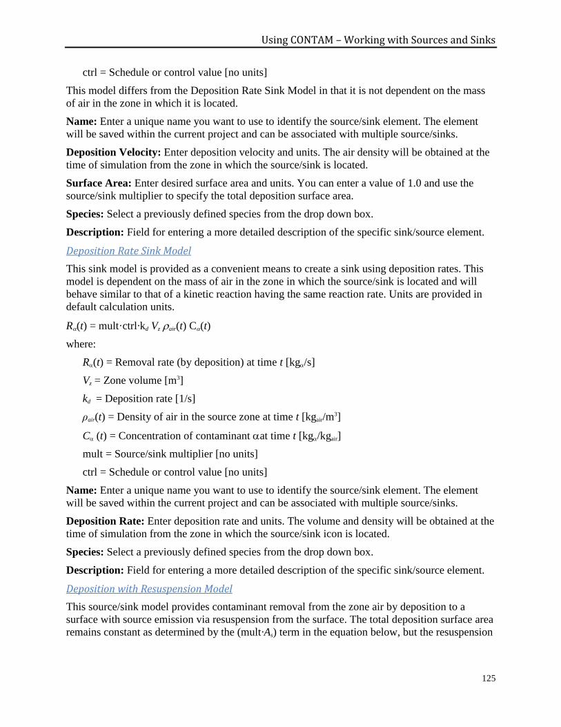
Using CONTAM – Working with Sources and Sinks
125
ctrl = Schedule or control value [no units]
This model differs from the Deposition Rate Sink Model in that it is not dependent on the mass
of air in the zone in which it is located.
Name: Enter a unique name you want to use to identify the source/sink element. The element
will be saved within the current project and can be associated with multiple source/sinks.
Deposition Velocity: Enter deposition velocity and units. The air density will be obtained at the
time of simulation from the zone in which the source/sink is located.
Surface Area: Enter desired surface area and units. You can enter a value of 1.0 and use the
source/sink multiplier to specify the total deposition surface area.
Species: Select a previously defined species from the drop down box.
Description: Field for entering a more detailed description of the specific sink/source element.
Deposition Rate Sink Model
This sink model is provided as a convenient means to create a sink using deposition rates. This
model is dependent on the mass of air in the zone in which the source/sink is located and will
behave similar to that of a kinetic reaction having the same reaction rate. Units are provided in
default calculation units.
R(t) = mult·ctrl·kd Vzair(t) C(t)
where:
R(t) = Removal rate (by deposition) at time t [kg/s]
Vz = Zone volume [m3]
kd = Deposition rate [1/s]
ρair(t) = Density of air in the source zone at time t [kgair/m3]
C (t) = Concentration of contaminant at time t [kg/kgair]
mult = Source/sink multiplier [no units]
ctrl = Schedule or control value [no units]
Name: Enter a unique name you want to use to identify the source/sink element. The element
will be saved within the current project and can be associated with multiple source/sinks.
Deposition Rate: Enter deposition rate and units. The volume and density will be obtained at the
time of simulation from the zone in which the source/sink icon is located.
Species: Select a previously defined species from the drop down box.
Description: Field for entering a more detailed description of the specific sink/source element.
Deposition with Resuspension Model
This source/sink model provides contaminant removal from the zone air by deposition to a
surface with source emission via resuspension from the surface. The total deposition surface area
remains constant as determined by the (mult·As) term in the equation below, but the resuspension
Using CONTAM – Working with Sources and Sinks
126
rate and area can be modified by a schedule or control value. Units are provided in default
calculation units.
R(t) = d (mult·As)air(t) C(t)
S(t) = (ctrl·r Ar) L(t)
where:
R(t) = Removal rate (by deposition) of contaminant from zone air to surface at time t
[kg/s]
vd = Deposition velocity [m/s]
As = Deposition surface area [m2]
ρair(t) = Density of air in the source zone at time t [kgair/m3]
C(t) = Concentration of contaminant in zone air volume at time t [kg/kgair]
S(t) = Source (resuspension) rate of contaminant from surface to zone air at time t [kg/s]
r = Resuspension rate [1/s]
Ar = Resuspension surface area [m2]
L(t) = Concentration of contaminant on the deposition surface at time t [kg/m2]
mult = Source/sink multiplier [no units]
ctrl = Schedule or control value [no units]
Name: Enter a unique name you want to use to identify the source/sink element. The element
will be saved within the current project and can be associated with multiple source/sinks.
Deposition Velocity: Enter deposition velocity and units. The air density will be obtained at the
time of simulation from the zone in which the source/sink is located.
Deposition Surface Area: Enter desired surface area and units. You can enter a value of 1.0 and
use the source/sink multiplier to specify the total deposition surface area for each specific
instance of this element.
Resuspension Rate: Enter the resuspension rate and units.
Resuspension Surface Area: The resuspension surface area may be different from that of the
deposition surface area, e.g., a shoe impacting the deposition surface. Once associated with a
source/sink, the resuspension rate can be varied using a schedule or control also associated with
the source/sink.
Species: Select a previously defined species from the drop down box.
Description: Field for entering a more detailed description of the specific sink/source element.
Using CONTAM – Working with Sources and Sinks
127
Super Source/Sink Element
Combine multiple sub-elements into a single element that can be represented by a single icon on
the SketchPad.
Name: Enter a unique name you want to use to identify the source/sink element. The element
will be saved within the current project and can be associated with multiple source/sinks.
Description: Field for entering a more detailed description of the specific sink/source element.
Available Elements: This is a list of basic source/sink elements from which you can build the
super element. Items below this list provide information on the currently highlighted element.
Use the Edit and New buttons to modify or create basic types of source/sink elements for the list
of available elements.
Sub-Elements: Use the Add and Remove buttons to modify this list of sub-elements that make
up the super element.
NRCC – Power Law Model
This is an empirically based model provided for compatibility with NRCC Material Emission
Database [Howard-Reed 2004 and 2006].
For t tp the initial emission factor is
So(t) = mult·a tp-b
and for t > tp
S(t) = mult·a t -b
NOTE: This type of source can only be triggered once per simulation. If using a schedule, the
first non-zero schedule value will trigger the source, otherwise it will begin emitting
immediately.
Name: Enter a unique name you want to use to identify the source/sink element. The element
will be saved within the current project and can be associated with multiple source/sinks.
Initial Emission Factor: Enter the initial emission factor S0 and its units [kg/s].
Coefficient: This corresponds to a in the above equation. It will be calculated based on S0, tp and
b. The value of a will be provided by the NRCC Data Base and stored by CONTAM, but the
Initial Emission Factor is provided as a more intuitive means for defining the model.
Exponent: Enter a value for the exponent b in the above equation.
PL Model Time: Enter the time tp until which the initial emission rate applies.
Description: Field for entering a more detailed description of the specific sink/source element.
NRCC - Peak Model
This is an empirically based model provided for compatibility with NRCC Material Emission
Database [Howard-Reed 2004 and 2006].
S(t) = mult·a·exp{-0.5[(1/b)·ln(t/tp)]2}
where:

Using CONTAM – Working with Sources and Sinks
128
a, b and tp are empirical coefficients typically determined from emission chamber
measurements.
The emission rate, S(t) [kg/s], will increase up until time tp at which point it will begin to
decay.
mult = Source/sink multiplier [no units]
NOTE: This type of source can only be triggered once per simulation. If using a schedule, the
first non-zero schedule value will trigger the source, otherwise it will begin emitting
immediately.
Name: Enter a unique name you want to use to identify the source/sink element. The element
will be saved within the current project and can be associated with multiple source/sinks.
Peak Emission Factor: Enter the peak emission factor a. This is the value of S(t) when time t =
tp.
Fitting Parameter: Enter a value for the parameter b in the above equation.
Time of Peak: Enter the time tp at which the peak emission factor is achieved.
Description: Field for entering a more detailed description of the specific source/sink element.
Using CONTAM – Working with Filters
129
3.11 WORKING WITH FILTERS
CONTAM provides some building components with the ability to incorporate filters that act as
contaminant removal devices. Filters consist of two parts: the filter itself which is associated
with a specific building component (path or duct segment) and filter elements that you can
associate with one or more filters. Filter elements provide the physical characteristics of the filter
and the mathematical relationship that describes the behavior of the filter during a simulation.
This is similar in nature to the relationship between airflow paths and airflow elements and
between duct segments and duct flow elements. In another sense, the filter is a specific instance
of a filter element.
The following building components can incorporate filters and are described as filter-ready:
1. Airflow paths
2. Implicit outdoor air and recirculation air paths of simple air-handling systems
3. Supplies and returns of simple air-handling systems
4. Duct segments
5. Duct terminals
3.11.1 Filter Elements
CONTAM uses mathematical relationships referred to as filter elements or models to implement
filters when performing contaminant simulations. CONTAM can implement several different
filter models to remove contaminants as they are transported through building components that
have filtering capabilities. These element types are described in detail in the Filter Element
Types section. Every filter must refer to a single filter element; however, multiple filters can
refer to the same filter element.
Filter elements can also be stored within a CONTAM library file and shared between different
CONTAM project files (See Working with Data and Libraries).
3.11.2 Creating Filters
You create filters for each building component for which you require a filter. When you are
defining one of the filter-ready building components presented above, a filter property page will
be provided that will enable you to establish whether or not to associate a filter, or to modify or
delete a previously defined filter for that component.
3.11.3 Deleting Filters
You can delete filters by accessing the properties of the individual component whose filter you
want to delete or by deleting the building component itself. Note that deleting a filter does not
delete the associated filter element (you can not delete a filter element that is currently associated
with a filter).
3.11.4 Modifying Filters
You modify a filter by accessing the Filter property page of the individual building component
icon and selecting the "Edit Filter" button to display the "Filter" dialog box.
Using CONTAM – Working with Filters
130
3.11.5 Filter Properties
Filter Number: This number is automatically assigned by ContamW and can change as you add
and remove filters to or from a project. Each time you save a project, the filter numbers are
reassigned.
Even though this is the actual filter number used by CONTAM, a different number will be used
when presenting filter accumulation results in the contaminant summary file (.csm file). This file
will present filters according to the building component with which they are associated. For
example, filters associated with airflow paths and air handling system supply and return points
will be referenced by the path number and the letter "p" to indicate it is a path filter. Filters
associated with ducts will be referenced by the duct segment number and the letter "d" or the
terminal number and the letter "t" for terminal.
Filter Element
Name: <required> You may select a previously defined filter element from those contained
in the Name list. Click the "New Element" button to define a new filter element. To view or
modify filter element data click the "Edit Element" button. You can also access the
CONTAM Library Manager to import filter elements from library files by clicking the
"Library" button (See Working with Data and Libraries). Every filter must have a filter
element associated with it.
Description: Displays the description of the filter element currently displayed in the Name
field.
Type: Displays the type of filter element for the filter currently displayed in the Name field.
Initial Filter Loading
Total Relative Load: Set the initial loading of the filter relative to the mass of the filter. This
can be set to zero to represent a "clean" filter at the beginning of a simulation; otherwise set
the value to establish the total mass of contaminants (as a percent of the mass of the filter)
accumulated on the filter at the start of a simulation. Relative load is only used for the
Gaseous Filter element which is currently the only element for which efficiency is described
as a function of filter loading.
3.11.6 Filter Element Types
These are the filter element types or models that you can implement with CONTAM. Refer to
the related information for each specific model for detailed descriptions.
Constant Efficiency Filter: Define constant efficiencies for each user-selected species.
Simple Particle Filter: Define filter efficiency as a function of particle size, for example a
MERV curve.
Simple Gaseous Filter: Define filter efficiency as a function of filter loading for a user
selectable set of species.
Penn State UVGI Filter: Define an ultra-violet germicidal irradiation filter.
Super Filter: This enables the combination of multiple filter elements into a single filter, e.g.,
a packaged filter that includes a gaseous filter and a pre-filter that filters particles.

Using CONTAM – Working with Filters
131
Constant Efficiency Filter
The constant efficiency filter element is made up of a set of species and associated efficiencies.
Each filter element can be associated with anywhere between one and the number of species that
exist within the current project. Only those species that you have selected to be contaminants will
be accounted for when you perform simulations.
Name: A unique name you want to use to identify the filter element.
Area: The face area and units of the filter element.
Depth: The depth of the filter element along the axis of airflow.
Density: The density of the filter media.
Area, Depth and Density are currently used to calculate the mass of the filter media which is only
relevant for the Simple Gaseous Filter model.
Description: Use this field to provide a more detailed description of the filter element.
Edit Element Data: Select to define the specific properties of the filter element.
Filtered Species: This is a list of the species and filter efficiencies for the filter element.
Edit Filter Data: Use the Species and Efficiency fields to set and modify the Filtered Species
list along with the Add, Replace and Delete command buttons.
Efficiency: Use this to enter the filter efficiency for the currently highlighted species. Filter
efficiencies must be between 0.0 and 1.0.
Species: This is a list of all the species in either the current project or library file depending
on wether you are editing project data or library data. Select the species for which you want
to set a filter efficiency.
Simple Particle Filter
The simple particle filter element consists of a single efficiency vs. particle size curve. In this
manner, a single filter element can be used to filter multiple particle contaminants based on
particle size alone. This can be used to define filters based on MERV test data [ASHRAE
1999a]. Only those species considered particle types and which you have selected to be
contaminants will be filtered when you perform simulations.
Name: A unique name you want to use to identify the filter element.
Area: The face area and units of the filter element.
Depth: The depth of the filter element along the axis of airflow.
Density: The density of the filter media.
Area, Depth and Density are currently used to calculate the mass of the filter media which is only
relevant for the Simple Gaseous Filter model.
Description: Use this field to provide a more detailed description of the filter element.
Edit Element Data: Select to define the specific properties of the filter element.
Filter Curve Data: This is a list of particle size and filter efficiency data pairs used to define
the filter curve. Once you have entered at least three data points, ContamW will attempt to
Using CONTAM – Working with Filters
132
calculate a cubic spline fit to the points. If there are any errors in the spline fit procedure, you
will be notified and the offending portion of the curve will be highlighted.
Use the Particle Size and Efficiency fields to set and modify the Filter Curve Data list along
with the Add, Replace and Delete command buttons.
Particle Size: Use this to enter the particle size and units for which to define a filter curve
data point. This corresponds to the Mean Diameter property of a species.
Efficiency: Use this to enter the filter efficiency for the associated particle size. Filter
efficiencies must be between 0.0 and 1.0.
At the beginning of a simulation, ContamX will use the curve to establish a filter efficiency
for each particle contaminant having a mean diameter in the range of the filter curve.
Simple Gaseous Filter
The simple gaseous filter element is made up of a set of species and associated efficiency vs.
loading curves. Therefore, the efficiency is a function of the amount of contaminant "absorbed"
by the filter. Each filter element can be associated with anywhere between one and the number of
species that exist within the current project. Only those species that you have selected to be
contaminants will be accounted for when you perform simulations.
Name: A unique name you want to use to identify the filter element.
Area: The face area and units of the filter element.
Depth: The depth of the filter element along the axis of airflow.
Density: The density of the filter media.
Area, Depth and Density are currently used to calculate the mass of the filter media which is in
turn used to calculate filter loading.
Description: Use this field to provide a more detailed description of the filter element.
Edit Element Data: Select to define the specific properties of the filter element.
Filter Curve Data: This is a list of relative loading and filter efficiency data pairs used to
define the filter curve for the currently selected species (see figure below). Once you have
entered at least three data points, ContamW will attempt to calculate a cubic spline fit to the
points. If there are any errors in the spline fit procedure, you will be notified and the
offending portion of the curve will be highlighted.

Using CONTAM – Working with Filters
133
Species: This is a list of all the species in either the current project or library file depending
on whether you are editing project data or library data. Select the species for which you want
to display/edit filter curve data.
Breakthrough Efficiency: Set the breakthrough efficiency for each species. This value will
be used during simulation to report if and when the filter efficiency drops below this value.
Breakthrough is reported to the Contaminant Summary simulation result file (see Results
Files in the Working with Results section).
Filter Curve Data: This is the list of data points you create from which a filter curve is
generated using the cubic spline fit method. A minimum of four data points is required before
a curve will be generated. The space below will provide a plot of Relative Loading vs. Filter
Efficiency. Relative loading is the ratio of Mass of contaminant accumulated by the filter to
the Mass of the filter.
Use the Relative Loading and Efficiency data entry fields to set and modify the Filter Curve
Data list along with the Add and Delete buttons.

Using CONTAM – Working with Filters
134
Penn State UVGI Filter
The Penn State UVGI element implements an ultra-violet germicidal irradiation filter model
based on work performed by the Pennsylvania State University [Lau 2009a, Lau 2009b]. The
filter efficiency, i.e., UV output, is a function of temperature, velocity (airflow rate), the age of
the filter relative and design UV output rate. The units provided below are those utilized
internally by ContamX.
Name: A unique name you want to use to identify this filter element.
Area, Depth and Density are used to calculate the mass of the filter media, which is not used for
this UVGI filter model, so these inputs can be ignored.
Description: Use this field to provide a more detailed description of the filter element.
Edit Element Data: Select to define the specific properties of this filter element. Units are
provided in the default calculation units.
Design Survivability, Sdesign: Enter the desired survivability of the filter as a fraction between
0 and 1.0. The single pass filter inactivation efficiency is equal to 1 - S.
Design Velocity, udesign [m/s]: Enter the design maximum velocity expected through the filter
flow region.
Design Organism-Specific Rate Constant, kdesign [m2/J]: Enter the design minimum
microorganism-specific rate constant. This will be used to determine the design UV dose.
You will also need to enter a value for each species that you want filtered by this UVGI filter
element (see Species Properties).
Design Mass Flow Rate, Fdes [kg/s]: Enter the design maximum airflow rate expected
through the filter flow region. This will be used along with the Design Velocity to calculate
the Cross-Sectional Flow Area.
Cross-sectional Flow Area, A [m2]: A = Fdesign / (std udesign)
Design Dose, (It)design [J/m2]: (It)design= ln(Sdesign)/-kdesign
TU Constants: C0 through C4 are used to determine the output as a percentage of design,
OUTTU, based on current conditions including flow velocity and temperature.
Use Age Model: Select this option to have the output also determined as a function of lamp
age.
Age Constants: K0 and K1 are the coefficients used to determine the percentage of output,
OUTage, based on the lamp age function.
Background In its simplest form, survivability of an airborne microorganism exposed to UV-C radiation, S,
presented in equation (uv-1), is approximated by a single-stage exponential decay equation [Lee
and Bahnfleth 2013].
(uv-1)
Efficiency is then 1 minus the survivability.
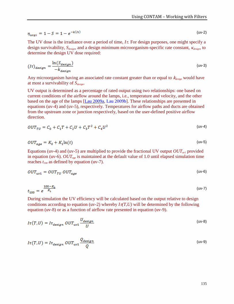
Using CONTAM – Working with Filters
135
(uv-2)
The UV dose is the irradiance over a period of time, I. For design purposes, one might specify a
design survivability, Sdesign, and a design minimum microorganism-specific rate constant, design, to
determine the design UV dose required:
(uv-3)
Any microorganism having an associated rate constant greater than or equal to kdesign would have
at most a survivability of Sdesign.
UV output is determined as a percentage of rated output using two relationships: one based on
current conditions of the airflow around the lamps, i.e., temperature and velocity, and the other
based on the age of the lamps [Lau 2009a, Lau 2009b]. These relationships are presented in
equations (uv-4) and (uv-5), respectively. Temperatures for airflow paths and ducts are obtained
from the upstream zone or junction respectively, based on the user-defined positive airflow
direction.
(uv-4)
(uv-5)
Equations (uv-4) and (uv-5) are multiplied to provide the fractional UV output OUTuv1 provided
in equation (uv-6). OUTage is maintained at the default value of 1.0 until elapsed simulation time
reaches t100 as defined by equation (uv-7).
(uv-6)
(uv-7)
During simulation the UV efficiency will be calculated based on the output relative to design
conditions according to equation (uv-2) whereby I(T,U) will be determined by the following
equation (uv-8) or as a function of airflow rate presented in equation (uv-9).
(uv-8)
(uv-9)
Using CONTAM – Working with Filters
136
Super Filter
Use this element to combine multiple filter elements, in series, into a single filter.
Name: A unique name you want to use to identify the super filter element.
Description: Use this field to provide a more detailed description of the filter element.
Sub-Elements: You build this list of sub-elements from the list of Available Elements The order
in which these elements appear in the list is important. They should be placed in the order in
which air is to flow through the filter from top to bottom in the list. Use the Add, Delete and
Move buttons to modify this list.
Available Elements: This is the list of fundamental filter elements, e.g., constant efficiency,
simple gaseous, and simple particle, contained in the current project file. Use the Edit Element
and New Element buttons to modify this list.

Using CONTAM – Working with Kinetic Reactions
137
3.12 WORKING WITH KINETIC REACTIONS
CONTAM provides the ability to model chemical reactions among project contaminants within
zones of a building including the implicit supply and return nodes of a simple air-handling
system (See Air Handling System). Kinetic reactions in CONTAM are modeled as first-order
exponential functions between species that contain the paired first-order reaction rate coefficients
between the reactant and product contaminants. See Axley [1988] and Axley [1995] for a
detailed presentations of the kinetic reaction simulation method employed by ContamX. The
production or destruction of a contaminant is given by
where
R rate of production or destruction of contaminant
K, reaction rate coefficients between contaminants and , in units of 1/s
C concentration of a reactant
CONTAM uses the convention that positive reaction coefficients produce an increase in species
concentration and negative coefficients decrease species concentrations. The units of
concentration are kg_species / kg_air (See Concentration Conversions).
Kinetic reactions can occur within zones of a building. To use kinetic reactions, you must have at
least one species for the project. Kinetic reactions can be associated with one or more zones
within a project. You can access the kinetic reaction data dialog box via the property sheets of
the zones that provide a kinetic reaction definition section (i.e. zones and simple air-handling
systems).
You can also access the Kinetic Reaction Data dialog box using the CONTAMW Data and
Library Manager: Kinetic Reactions to create and edit local project data or to share kinetic
reactions between CONTAM projects using contaminant libraries.
When you are defining building zones, you will be able to select a currently defined kinetic
reaction to associate with it, define new, modify existing or import kinetic reactions from
species-related CONTAM library files (i.e. LB0 library files). All kinetic reactions are defined
and modified using the Kinetic Reaction Data dialog box as described in the following section.
Kinetic Reaction Data
Kinetic reaction elements are made up of source/product species pairs. You can define any
number of pairs per element you desire. Only those species that you have selected to be
contaminants will be accounted for when you perform simulations. These are the properties that
describe a kinetic reaction.
Name: Enter a unique name you want to use to identify the reaction matrix. You will use this
name to associate this element with zones within the project.
Description: Use this to provide a more detailed description of the kinetic reaction.
Reactant→Product Pairs: This is a list of the reactant/product pairs and their associated
reaction coefficients that are currently defined for the current kinetic reaction element.
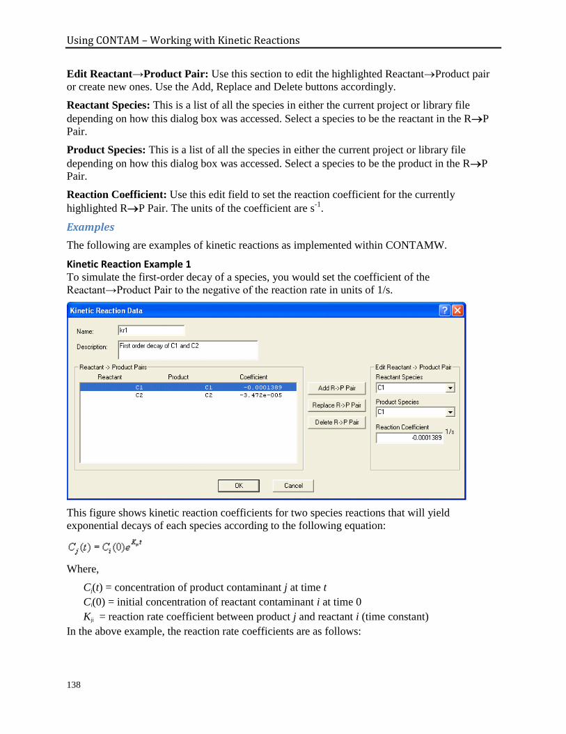
Using CONTAM – Working with Kinetic Reactions
138
Edit Reactant→Product Pair: Use this section to edit the highlighted ReactantProduct pair
or create new ones. Use the Add, Replace and Delete buttons accordingly.
Reactant Species: This is a list of all the species in either the current project or library file
depending on how this dialog box was accessed. Select a species to be the reactant in the RP
Pair.
Product Species: This is a list of all the species in either the current project or library file
depending on how this dialog box was accessed. Select a species to be the product in the RP
Pair.
Reaction Coefficient: Use this edit field to set the reaction coefficient for the currently
highlighted RP Pair. The units of the coefficient are s-1
.
Examples
The following are examples of kinetic reactions as implemented within CONTAMW.
Kinetic Reaction Example 1 To simulate the first-order decay of a species, you would set the coefficient of the
Reactant→Product Pair to the negative of the reaction rate in units of 1/s.
This figure shows kinetic reaction coefficients for two species reactions that will yield
exponential decays of each species according to the following equation:
Where,
Cj(t) = concentration of product contaminant j at time t
Ci(0) = initial concentration of reactant contaminant i at time 0
Kji = reaction rate coefficient between product j and reactant i (time constant)
In the above example, the reaction rate coefficients are as follows:
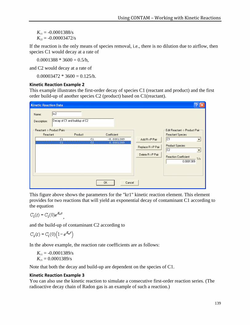
Using CONTAM – Working with Kinetic Reactions
139
K11 = -0.0001388/s
K22 = -0.00003472/s
If the reaction is the only means of species removal, i.e., there is no dilution due to airflow, then
species C1 would decay at a rate of
0.0001388 * 3600 = 0.5/h,
and C2 would decay at a rate of
0.00003472 * 3600 = 0.125/h.
Kinetic Reaction Example 2 This example illustrates the first-order decay of species C1 (reactant and product) and the first
order build-up of another species C2 (product) based on C1(reactant).
This figure above shows the parameters for the "kr1" kinetic reaction element. This element
provides for two reactions that will yield an exponential decay of contaminant C1 according to
the equation
,
and the build-up of contaminant C2 according to
In the above example, the reaction rate coefficients are as follows:
K11 = -0.0001389/s
K21 = 0.0001389/s
Note that both the decay and build-up are dependent on the species of C1.
Kinetic Reaction Example 3 You can also use the kinetic reaction to simulate a consecutive first-order reaction series. (The
radioactive decay chain of Radon gas is an example of such a reaction.)
Using CONTAM – Working with Kinetic Reactions
140
A two-step consecutive reaction series involving a single reactant at each step is indicated as
C1 C2
C2 products
You would model this reaction chain by inputing coefficients based on the half-life of the
radioactive reactants. Convert half-life 1/2 to a first-order reaction coefficient, K21, using the
following equation:
In CONTAM, you would require two species C1 and C2 (if interested in contaminant C2) and
three reactant/product pairs have the following reaction coefficients characteristics:
K11 would have negative non-zero values (decay of C1)
K21 would have a non-zero positive value (build-up of C2 from C1)
K22 would have negative non-zero values (decay of C2)
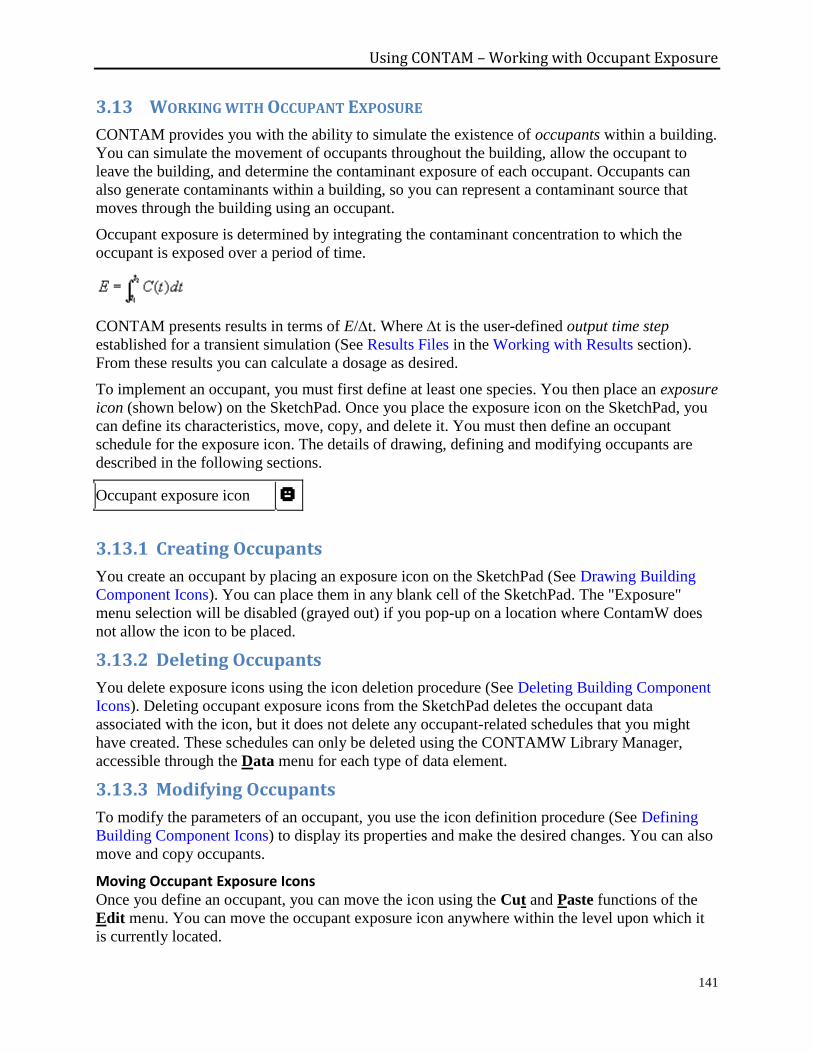
Using CONTAM – Working with Occupant Exposure
141
3.13 WORKING WITH OCCUPANT EXPOSURE
CONTAM provides you with the ability to simulate the existence of occupants within a building.
You can simulate the movement of occupants throughout the building, allow the occupant to
leave the building, and determine the contaminant exposure of each occupant. Occupants can
also generate contaminants within a building, so you can represent a contaminant source that
moves through the building using an occupant.
Occupant exposure is determined by integrating the contaminant concentration to which the
occupant is exposed over a period of time.
CONTAM presents results in terms of E/t. Where t is the user-defined output time step
established for a transient simulation (See Results Files in the Working with Results section).
From these results you can calculate a dosage as desired.
To implement an occupant, you must first define at least one species. You then place an exposure
icon (shown below) on the SketchPad. Once you place the exposure icon on the SketchPad, you
can define its characteristics, move, copy, and delete it. You must then define an occupant
schedule for the exposure icon. The details of drawing, defining and modifying occupants are
described in the following sections.
Occupant exposure icon
3.13.1 Creating Occupants
You create an occupant by placing an exposure icon on the SketchPad (See Drawing Building
Component Icons). You can place them in any blank cell of the SketchPad. The "Exposure"
menu selection will be disabled (grayed out) if you pop-up on a location where ContamW does
not allow the icon to be placed.
3.13.2 Deleting Occupants
You delete exposure icons using the icon deletion procedure (See Deleting Building Component
Icons). Deleting occupant exposure icons from the SketchPad deletes the occupant data
associated with the icon, but it does not delete any occupant-related schedules that you might
have created. These schedules can only be deleted using the CONTAMW Library Manager,
accessible through the Data menu for each type of data element.
3.13.3 Modifying Occupants
To modify the parameters of an occupant, you use the icon definition procedure (See Defining
Building Component Icons) to display its properties and make the desired changes. You can also
move and copy occupants.
Moving Occupant Exposure Icons Once you define an occupant, you can move the icon using the Cut and Paste functions of the
Edit menu. You can move the occupant exposure icon anywhere within the level upon which it
is currently located.

Using CONTAM – Working with Occupant Exposure
142
Copying Occupant Exposure Icons Once you define an occupant, you can copy the icon using the Copy and Paste functions of the
Edit menu. You can copy an occupant to any blank cell on any level of a project.
3.13.4 Defining Occupants
After you draw an exposure icon on the SketchPad you must define it using the icon definition
procedure (See Defining Building Component Icons) to display and edit the properties. This will
display the "Occupant Exposure Properties" dialog box. Detailed descriptions of all occupant
exposure properties are given in the following Occupant Properties section. Once you have
defined the properties, the icon will be displayed in black. From now on, you use this icon to
access the properties of the occupant.
3.13.5 Occupant Properties
This section provides detailed descriptions of the specific occupant properties including
occupancy schedule, i.e., location within the building over time and the occupant-associated
contaminant generation. Each of the following subsections are the context-sensitive help topics
that you can access by pressing F1 when working with property pages of the "Occupant
Exposure Properties" property sheet.
Occupant – Occupancy Schedule Properties
Occupant Number: This is the number that appears in the status bar when you highlight an
icon. ContamW automatically assigns this number to each exposure icon once it is defined. This
number could change as you add and remove occupants to or from a project. Each time you save
a project, the occupant numbers are reassigned. Numbers are assigned beginning on the top level,
starting from the upper-left corner of the SketchPad, moving left-to-right and top-to-bottom of
the SketchPad.
Occupant Week Schedule: Use the Occupancy Week Schedule to define the movement of this
occupant within the building (see Working with Schedules).
Occupant – Contaminant Generation Properties
Multiplier: Use the multiplier to modify the generation rate of an occupant. You could define
the contaminant generation rate(s) for a single occupant and use the multiplier to represent a
generation rate of multiple occupants.
Generate Contaminants: This checkbox is used to turn on and off the contaminant generation
of the occupant. If the box is checked, contaminants will be generated. This is useful for
contaminant generation such as that of carbon dioxide due to human metabolic activity.
Generation Data: A list of available contaminants is displayed in the text box provided. You
can highlight these contaminants and select the generation rate for each in the edit box below the
contaminant list.
Generation Schedule: A new inhalation schedule is defined by pressing the "New Schedule"
button and following the directions for editing a Week Schedule.
Description: Field that shows a more detailed description of the specific schedule if entered
by the user. This description can be modified by pressing the edit schedule button next to the
description field and then changing the description field for the schedule.
Using CONTAM – Working with Occupant Exposure
143
Name: This drop down box contains the names of all previously created schedules. The
schedule selected from this box will then define the generation schedule for the exposure
element being viewed.
CVF/DVF Control: Values from either a CVF or DVF file can be used in place of the above
Schedule (read about CVF and DVF controls in the Control Element Types section). This
enables using these control element types without having to draw/define an associated control
network. The associated radio buttons "Use Neither", "Use CVF" and "Use DVF" are used to
select the desired control method. Select the heading name from the associated "Name" drop
down box that will display the headings of either the CVF or DVF file as per the aforementioned
radio button selection.
Control Status: This will display the current method of control: Schedule, direct CVF, direct
DVF or Control Network. If an actuator of a control network on the SketchPad is associated with
the scheduled item then it will take precedence over the Schedule and CVF/DVF Control. If
either the "Use CVF" or "Use DVF" radio button is selected then CVF or DVF will take
precedence over an associated schedule.
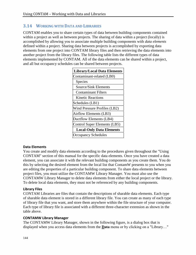
Using CONTAM – Working with Data and Libraries
144
3.14 WORKING WITH DATA AND LIBRARIES
CONTAM enables you to share certain types of data between building components contained
within a project as well as between projects. The sharing of data within a project (locally) is
accomplished by allowing you to associate multiple building components with data elements
defined within a project. Sharing data between projects is accomplished by exporting data
elements from one project into CONTAM library files and then retrieving the data elements into
another project from the library files. The following table lists the different types of data
elements implemented by CONTAM. All of the data elements can be shared within a project,
and all but occupancy schedules can be shared between projects.
Library/Local Data Elements
Contaminant-related (LB0)
Species
Source/Sink Elements
Contaminant Filters
Kinetic Reactions
Schedules (LB1)
Wind Pressure Profiles (LB2)
Airflow Elements (LB3)
Ductflow Elements (LB4)
Control Super Elements (LB5)
Local-Only Data Elements
Occupancy Schedules
Data Elements You create and modify data elements according to the procedures given throughout the "Using
CONTAM" section of this manual for the specific data elements. Once you have created a data
element, you can associate it with the relevant building components as you create them. You do
this by selecting the desired element from the local list that ContamW presents to you when you
are editing the properties of a particular building component. To share data elements between
project files, you must utilize the CONTAMW Library Manager. You must also use the
CONTAMW Library Manager to delete data elements from either the local project or the library.
To delete local data elements, they must not be referenced by any building components.
Library Files CONTAM Libraries are files that contain the descriptions of sharable data elements. Each type
of sharable data element is stored in a different library file. You can create as many of each type
of library file that you want, and store them anywhere within the file structure of your computer.
Each type of library file is associated with a different three-character extension as shown in the
table above.
CONTAMW Library Manager The CONTAMW Library Manager, shown in the following figure, is a dialog box that is
displayed when you access data elements from the Data menu or by clicking on a "Library…"
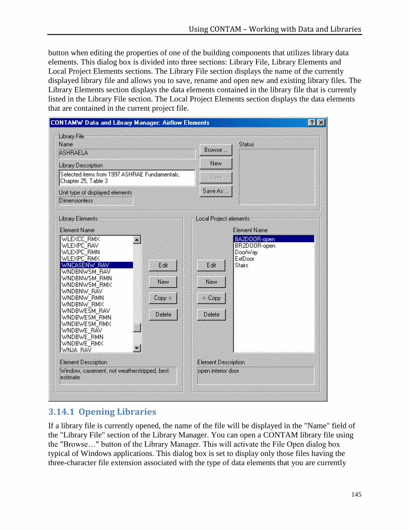
Using CONTAM – Working with Data and Libraries
145
button when editing the properties of one of the building components that utilizes library data
elements. This dialog box is divided into three sections: Library File, Library Elements and
Local Project Elements sections. The Library File section displays the name of the currently
displayed library file and allows you to save, rename and open new and existing library files. The
Library Elements section displays the data elements contained in the library file that is currently
listed in the Library File section. The Local Project Elements section displays the data elements
that are contained in the current project file.
3.14.1 Opening Libraries
If a library file is currently opened, the name of the file will be displayed in the "Name" field of
the "Library File" section of the Library Manager. You can open a CONTAM library file using
the "Browse…" button of the Library Manager. This will activate the File Open dialog box
typical of Windows applications. This dialog box is set to display only those files having the
three-character file extension associated with the type of data elements that you are currently
Using CONTAM – Working with Data and Libraries
146
working with. Follow the typical procedure for opening a file using the Windows operating
system.
CONTAM 2.0 library files are of a different format than the 1.0 version. ContamW will allow
you to open a 1.0 version file and you will then be required to give the file a name when saving
the converted file. It is suggested that you save the file under a different name from that of the
1.0 formatted library file. The Open dialog box will display both the file Version information and
the Library file description.
3.14.2 Creating Libraries
Using the CONTAMW Library Manager, you create new libraries one of two ways. You can
either save an existing library under a new name using the "Save As…" button, or use the "New"
button of the Library File section of the CONTAMW Library Manager dialog box. The "Save
As…" method makes a copy of the currently displayed library file under a new name, but
maintains the original file. The "New" method clears the data currently displayed and allows you
to start with an empty library file.
3.14.3 Deleting Libraries
You must use the file deletion commands of your operating system to delete CONTAM library
files.
3.14.4 Modifying Libraries
You modify CONTAM library files using the CONTAMW Library Manager. The CONTAMW
Library Manager allows you to create new data elements within the library, copy data elements
from the local project into the library, modify library data elements, and delete data elements
from the library.
Creating Library Data Elements You use the "New" button contained within the "Library Elements" section of the CONTAMW
Library Manager to create a new data element. You can only create the type of data element that
is currently being displayed by the Library Manager (e.g. airflow elements, ductflow elements,
schedules, etc. ). The "New" button will activate the ContamW dialog box associated with
creating the type of data element that you are currently working with.
Species must be available in order to create new contaminant-related elements such as
Sources/Sinks, Filters and Kinetic reactions.
Copying Library Data Elements (between the Project and Library) You can either copy data element from a library to the local project or from the local project to
the library. All copying is done between the local project and the library file that is currently
indicated in the "Name" box of the Library File section of the CONTAMW Library Manager. If
the name box is blank, then you are dealing with a new/unnamed library file. To copy data
elements, you use the "Copy →" and "← Copy" buttons. These copy buttons indicate the
direction of the copy operation. If an element exists in both the library file and the local project,
then the copy buttons will be disabled to prevent you from overwriting elements with the same
name. You may rename local data elements without affecting their associations with building
components that refer to them in the local project.
Using CONTAM – Working with Data and Libraries
147
Some elements rely on other types of elements for proper implementation, e.g., source/sinks
require an associated species and week schedules require day schedules. If you copy one of these
elements that requires a sub element, ContamW will prompt you to replace existing elements of
the same name if they already exist within the destination file.
Modifying Library Data Elements To modify a library data element, you must first highlight the Element Name within the list of
elements in the Library Elements section of the CONTAMW Library Manager. You then click
on the "Edit" button next to the list. This will activate the ContamW dialog box associated with
displaying the properties of the type of data element with which you are currently working. You
then make the desired changes and click the "OK" button to make the changes take affect.
Deleting Library Data Elements To delete a library data element, you highlight the Element Name in the Library Elements
section of the CONTAMW Library Manager then click on the "Delete" button next to the list.
You will be prompted to confirm the deletion, and the data element will no longer be displayed
in the list of Library Elements. However, the deletion will not be affected until you save the
library file. You can retrieve the previously deleted data elements by reopening the library file as
long as you don't save the file after deleting the elements.
Deleting data elements that have associated sub-elements will not delete the sub-elements. You
must delete the sub-elements using a separate Library Manager operation.
3.14.5 Modifying Local Data
You modify local lists of data elements using the CONTAMW Library Manager. The Library
Manager allows you to create new local data elements, copy data elements from the library into
the local project, modify local data elements, and delete local data elements.
Creating Local Data Elements You use the "New" button contained within the "Project Elements" section of the Library
Manager to create a new data element. You can only create the type of data element that is
currently being displayed by the Library Manager (e.g. airflow elements, ductflow elements,
schedules, etc. ). The "New" button will activate the ContamW dialog box associated with
creating the type of data element that you are currently working with.
Species must be available in order to create new contaminant-related elements such as
Sources/Sinks, Filters and Kinetic reactions.
Copying Local Data Elements (between the Project and Library) See Copying Library Data Elements.
Modifying Local Data Elements The Library Manager provides you with another means of accessing local project elements. This
is in addition to the method of accessing building component properties presented throughout the
Using CONTAM section of this manual. You must first highlight the Element Name within the
list of elements in the Project Elements section of the Library Manager. You then click on the
"Edit" button next to the list. This will activate the ContamW dialog box associated with
displaying the properties of the type of data element that you are currently working with. You
then make the desired changes and click the "OK" button to make the changes take affect.
Using CONTAM – Working with Data and Libraries
148
Copying Data Elements (within a Project) You can use the Library Manager to create elements that are similar to existing elements but
have a different name. To do this you copy a project element to the library (you don’t have to
have an existing library file open), give the library element a new name, make the modifications
you desire and copy the element back into your project.
Deleting Local Data Elements You can only delete local data elements if they are not referenced by any building components
within the project. To delete a project data element, you highlight the Element Name in the
Project Elements section of the CONTAMW Library Manager then click on the "Delete" button
next to the list. The "Delete" button will only be enabled if the currently highlighted element is
not referenced within the project. You will be prompted to confirm the deletion, and the data
element will no longer be displayed in the list of Project Elements. However, the deletion will
not be affected until you save the project file. You can retrieve the previously deleted data
elements by reopening the project file as long as you don't save the file after deleting the
elements.
Deleting data elements that have associated sub-elements will not delete the sub-elements. You
must delete the sub-elements using a separate Library Manager operation.

Using CONTAM – Working with Weather and Wind
149
3.15 WORKING WITH WEATHER AND WIND
CONTAM enables you to incorporate the effects of weather on a building. Weather parameters
include ambient temperature, barometric pressure, wind speed, wind direction and also outdoor
contaminant levels. The type of weather data you require for a simulation depends on the type of
simulation you are performing, whether you want to account for the effects of wind, and whether
or not you are simulating contaminants. If you are performing a steady-state airflow simulation,
you will only need steady state weather and wind data. If you are performing a transient airflow
simulation, you can use either steady state or transient weather data. Transient weather data is
implemented through the use of weather files or WTH files. If you are performing transient
contaminant simulations, you can use either steady-state or transient ambient contaminant data as
well. Transient ambient contaminant data is implemented via the use of ambient contaminant
files or CTM files (See Contaminant Files).
NOTE: Both the WTH and CTM files assume a single set of values for the ambient zone at any
given point in time, i.e., there is no spacial variation in either the pressure or contaminant fields.
However, CONTAM also allows the use of transient wind pressure and contaminant files (WPC
file) with which you can account for spacial variation in both the pressures and contaminant
concentrations over the surface of a building envelope (See Working with WPC Files).
Steady State Weather When you use steady state weather data, ContamX keeps the ambient temperature, barometric
pressure, wind speed and direction and relative humidity constant during a simulation. Detailed
descriptions of these parameters are given in the following sections.
Transient Weather You can use transient weather data to simulate the changing outdoor weather and wind
conditions when performing a transient simulation. Transient weather data is stored in a weather
file that you must create according to a special format as specified under the Weather File
Format section that follows. Weather files contain ambient temperature, pressure, wind speed
and direction and humidity ratio for discrete intervals of each day for at least one day and up to
one year. If the intervals between data in the weather file don't match the simulation time step,
ContamX will linearly interpolate the weather data to obtain a value at the required timestep.
Wind Wind pressure can be a significant driving force for air infiltration through a building envelope.
It is a function of wind speed, wind direction, building configuration, and local terrain effects.
CONTAM enables you to account for the effects of wind pressure on flow paths through the
building envelope (external airflow paths). You define how you want to account for wind effect
for each external flow path on a case-by-case basis. In ContamW, you can either choose to
ignore the effects of wind on an envelope penetration, define wind pressure to be constant for
each envelope penetration, or implement variable wind pressures for envelope penetrations.
CONTAM provides a general approach to handling the variable effects of wind on the building
envelope. This approach requires you to provide CONTAM with information related to the
determination of a local wind pressure coefficient for the building surface.
For a general introduction to the effects of wind pressure on buildings, see Chapter 16, Air flow
Around Buildings, in the 2005 ASHRAE Fundamentals Handbook [ASHRAE 2005]. The
following is an overview of how CONTAM handles these effects.
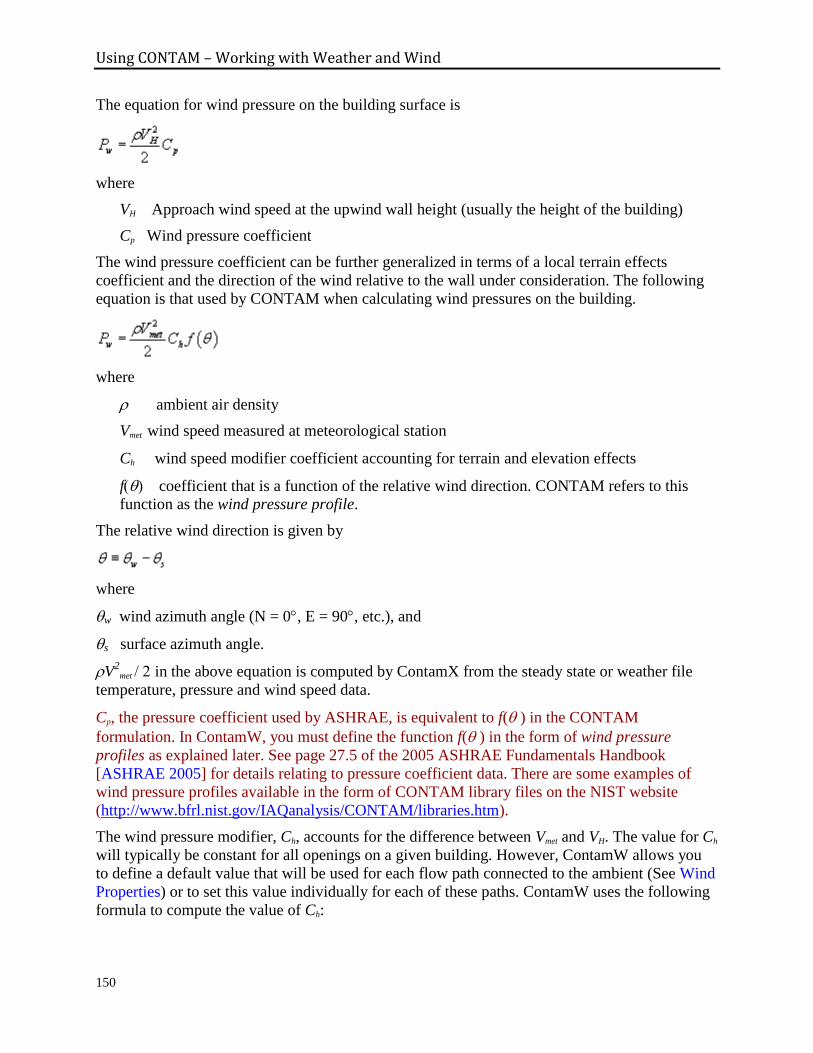
Using CONTAM – Working with Weather and Wind
150
The equation for wind pressure on the building surface is
where
VH Approach wind speed at the upwind wall height (usually the height of the building)
Cp Wind pressure coefficient
The wind pressure coefficient can be further generalized in terms of a local terrain effects
coefficient and the direction of the wind relative to the wall under consideration. The following
equation is that used by CONTAM when calculating wind pressures on the building.
where
ambient air density
Vmet wind speed measured at meteorological station
Ch wind speed modifier coefficient accounting for terrain and elevation effects
f coefficient that is a function of the relative wind direction. CONTAM refers to this
function as the wind pressure profile.
The relative wind direction is given by
where
w wind azimuth angle (N = 0, E = 90, etc.), and
s surface azimuth angle.
V2
met in the above equation is computed by ContamX from the steady state or weather file
temperature, pressure and wind speed data.
Cp, the pressure coefficient used by ASHRAE, is equivalent to f( ) in the CONTAM
formulation. In ContamW, you must define the function f() in the form of wind pressure
profiles as explained later. See page 27.5 of the 2005 ASHRAE Fundamentals Handbook
[ASHRAE 2005] for details relating to pressure coefficient data. There are some examples of
wind pressure profiles available in the form of CONTAM library files on the NIST website
(http://www.bfrl.nist.gov/IAQanalysis/CONTAM/libraries.htm).
The wind pressure modifier, Ch, accounts for the difference between Vmet and VH. The value for Ch
will typically be constant for all openings on a given building. However, ContamW allows you
to define a default value that will be used for each flow path connected to the ambient (See Wind
Properties) or to set this value individually for each of these paths. ContamW uses the following
formula to compute the value of Ch:
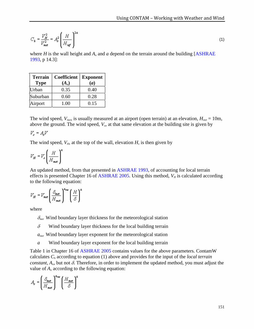
Using CONTAM – Working with Weather and Wind
151
(1)
where H is the wall height and Ao and a depend on the terrain around the building [ASHRAE
1993, p 14.3]:
Terrain
Type
Coefficient
(Ao)
Exponent
(a)
Urban 0.35 0.40
Suburban 0.60 0.28
Airport 1.00 0.15
The wind speed, Vmet, is usually measured at an airport (open terrain) at an elevation, Hmet = 10m,
above the ground. The wind speed, Vo, at that same elevation at the building site is given by
The wind speed, VH, at the top of the wall, elevation H, is then given by
An updated method, from that presented in ASHRAE 1993, of accounting for local terrain
effects is presented Chapter 16 of ASHRAE 2005. Using this method, VH is calculated according
to the following equation:
where
met Wind boundary layer thickness for the meteorological station
Wind boundary layer thickness for the local building terrain
amet Wind boundary layer exponent for the meteorological station
a Wind boundary layer exponent for the local building terrain
Table 1 in Chapter 16 of ASHRAE 2005 contains values for the above parameters. ContamW
calculates Ch according to equation (1) above and provides for the input of the local terrain
constant, Ao, but not . Therefore, in order to implement the updated method, you must adjust the
value of Ao according to the following equation:
Using CONTAM – Working with Weather and Wind
152
3.15.1 Defining Weather and Wind
You define weather that you want CONTAM to use based on the type of simulation you want to
perform. You will either define steady state weather or transient weather. It is best to perform a
set of steady state simulations prior to performing transient simulations. This may enable you to
better identify any problems that may arise from working with transient weather. ContamW also
provides a means to verify that you have your wind related data input correctly (See Checking
Wind Pressure Data).
Defining Steady State Weather and Wind
To define the steady state weather and wind data you use the Edit Weather Data… selection of
the Weather menu or the F7 keyboard shortcut. This will display the "Weather and Wind
Parameters" property sheet. The property sheet contains four different pages of parameters
including: Weather, Wind, Location and Wind Pressure Display. Detailed descriptions of all
wind and weather properties are given in the Weather and Wind Properties section of this
manual.
You use the Weather page to define steady state weather and wind data. The Location page
allows you to input the altitude of the building site which ContamW will use to determine a
default barometric pressure if you do not know what it should be for a given building site.
Default values of these two pages will provide conditions of no wind, 20 °C and a barometric
pressure of 1 atmosphere (approximately 101 kPa).
The Wind page parameters allow you to enter the prevailing wind direction and other values
used by ContamW to determine a wind speed modifier. The wind speed modifier is determined
from the local terrain constant and the velocity profile exponent. Default values are provided for
suburban terrain.
Checking Wind Pressure Data ContamW enables you to verify wind information visually on the SketchPad using the Wind
Pressure and Wind Pressure Type selections of the View menu. When reviewing this display,
you should check if the direction of flow makes sense based on the wind data provided on the
Wind Pressure Display property page (WP Display) or contained in the WTH and WPC file (see
Working with WPC Files). When reviewing WTH and WPC file pressures, you can use the
Results Navigation controls under the View menu to step through the data in the WPC file. The
date and time of the corresponding data from either file will be displayed in the status bar.
When you choose to display wind pressure results, colored lines (Pres Results color) will appear
on the SketchPad. Wind pressure will only be displayed for those airflow paths and duct
terminals connected to the ambient zone, having the Wind Pressure Option set to Variable or
Constant or, if using a WPC file, a pressure specified in the WPC file. The wind pressure display
will reveal the relative magnitude of the pressure drop and the direction of airflow across the
openings in the building envelope. You can move the caret to each of the airflow paths for which
a wind pressure is being displayed to show the wind pressure, azimuth angle and elevation of the
airflow path in the ContamW status bar. When the caret is placed in the ambient zone, the wind
speed and direction will be displayed in the status bar if the wind pressure type is set to either
WP Display or WTH.
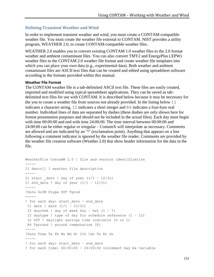
Using CONTAM – Working with Weather and Wind
153
Defining Transient Weather and Wind
In order to implement transient weather and wind, you must create a CONTAM-compatible
weather file. You must create the weather file external to CONTAM. NIST provides a utility
program, WEATHER 2.0, to create CONTAM-compatible weather files.
WEATHER 2.0 enables you to convert existing CONTAM 1.0 weather files to the 2.0 format
weather and ambient contaminant files. You can also convert TMY2 and EnergyPlus (.EPW)
weather files to the CONTAM 2.0 weather file format and create weather file templates into
which you can place your own data (e.g., experimental data). Both weather and ambient
contaminant files are ASCII text files that can be created and edited using spreadsheet software
according to the formats provided within this manual.
Weather File Format The CONTAM weather file is a tab-delimited ASCII text file. These files are easily created,
imported and modified using typical spreadsheet applications. They can be saved as tab-
delimited text files for use with CONTAM. It is described below because it may be necessary for
the you to create a weather file from sources not already provided. In the listing below I1
indicates a character string, I2 indicates a short integer and R4 indicates a four-byte real
number. Individual lines of data are separated by dashes (these dashes are only shown here for
format presentation purposes and should not be included in the actual files). Each day must begin
with time 00:00:00 and end with time 24:00:00. The time interval between 00:00:00 and
24:00:00 can be either regular or irregular – ContamX will interpolate as necessary. Comments
are allowed and are indicated by an "!" (exclamation point). Anything that appears on a line
following a comment indicator is ignored by the weather file reader. Comments are provided by
the weather file creation software (Weather 2.0) that show header information for the data in the
file.
WeatherFile ContamW 2.0 ! file and version identification
-----
I1 descr[] ! weather file description
-----
I1 start _date ! day of year (1/1 – 12/31)
I1 end_date ! day of year (1/1 – 12/31)
-----
!Date DofW Dtype DST Tgrnd
-----
! for each day: start_date – end_date
I1 date ! date (1/1 – 12/31)
I2 dayofwk ! day of week Sun – Sat (1 - 7)
I2 daytype ! type of day for schedule reference (1 – 12)
I2 DST ! daylight savings time indicator (0 or 1)
R4 Tground ! ground temperature [K]
-----
!Date Time Ta Pb Ws Wd Hr Ith Idn Ts Rn Sn
-----
! for each day: start_date – end_date
! for each time: 00:00:00 - 24:00:00 increment may be variable
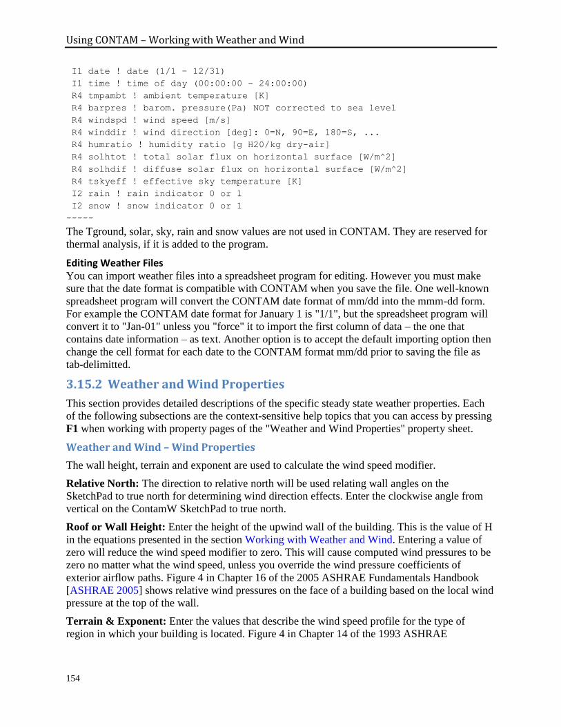
Using CONTAM – Working with Weather and Wind
154
I1 date ! date (1/1 – 12/31)
I1 time ! time of day (00:00:00 – 24:00:00)
R4 tmpambt ! ambient temperature [K]
R4 barpres ! barom. pressure(Pa) NOT corrected to sea level
R4 windspd ! wind speed [m/s]
R4 winddir ! wind direction [deg]: 0=N, 90=E, 180=S, ...
R4 humratio ! humidity ratio [g H20/kg dry-air]
R4 solhtot ! total solar flux on horizontal surface [W/m^2]
R4 solhdif ! diffuse solar flux on horizontal surface [W/m^2]
R4 tskyeff ! effective sky temperature [K]
I2 rain ! rain indicator 0 or 1
I2 snow ! snow indicator 0 or 1
-----
The Tground, solar, sky, rain and snow values are not used in CONTAM. They are reserved for
thermal analysis, if it is added to the program.
Editing Weather Files You can import weather files into a spreadsheet program for editing. However you must make
sure that the date format is compatible with CONTAM when you save the file. One well-known
spreadsheet program will convert the CONTAM date format of mm/dd into the mmm-dd form.
For example the CONTAM date format for January 1 is "1/1", but the spreadsheet program will
convert it to "Jan-01" unless you "force" it to import the first column of data – the one that
contains date information – as text. Another option is to accept the default importing option then
change the cell format for each date to the CONTAM format mm/dd prior to saving the file as
tab-delimitted.
3.15.2 Weather and Wind Properties
This section provides detailed descriptions of the specific steady state weather properties. Each
of the following subsections are the context-sensitive help topics that you can access by pressing
F1 when working with property pages of the "Weather and Wind Properties" property sheet.
Weather and Wind – Wind Properties
The wall height, terrain and exponent are used to calculate the wind speed modifier.
Relative North: The direction to relative north will be used relating wall angles on the
SketchPad to true north for determining wind direction effects. Enter the clockwise angle from
vertical on the ContamW SketchPad to true north.
Roof or Wall Height: Enter the height of the upwind wall of the building. This is the value of H
in the equations presented in the section Working with Weather and Wind. Entering a value of
zero will reduce the wind speed modifier to zero. This will cause computed wind pressures to be
zero no matter what the wind speed, unless you override the wind pressure coefficients of
exterior airflow paths. Figure 4 in Chapter 16 of the 2005 ASHRAE Fundamentals Handbook
[ASHRAE 2005] shows relative wind pressures on the face of a building based on the local wind
pressure at the top of the wall.
Terrain & Exponent: Enter the values that describe the wind speed profile for the type of
region in which your building is located. Figure 4 in Chapter 14 of the 1993 ASHRAE
Using CONTAM – Working with Weather and Wind
155
Fundamentals Handbook [ASHRAE 1993] shows terrain constants and velocity profile
exponents for representative areas.
An updated method, from that presented in ASHRAE 1993, of accounting for local terrain
effects is presented Chapter 16 of ASHRAE 2005. Refer to Working with Weather and Wind for
details on how to implement this method within CONTAM.
Modifier: This is the wind speed modifier, Ch, calculated by ContamW based on the Wall
Height, Terrain and Exponent values above. This value will be the default provided for each
envelope airflow path that you create on the SketchPad and for which you select the variable
wind pressure option. See section Working with Weather and Wind for a more detailed
explanation of this term.
Weather and Wind – Weather Properties
The following constant values are used by CONTAM when you specify the use of steady state
weather conditions when performing simulations (See Working with Simulations).
Temperature: ContamX uses the ambient temperature when calculating outside air density and
building stack effects.
Absolute Pressure: Absolute barometric pressure (not corrected to sea level). If you don't know
this value, you can enter the altitude of the building site on the Location Properties page to have
ContamW calculate the barometric pressure for you.
Relative Humidity: Relative humidity as a fraction, i.e., between 0.0 and 1.0. This value will be
used along with Ambient Temperature and Pressure to calculate the Humidity Ratio and Mass
Fraction of H2O.
Humidity Ratio: The mass of water vapor per mass of air (excluding water vapor) calculated
based on the Temperature, Pressure and Relative Humidity.
Humidity Ratio = Mass Fraction / (1 – Mass Fraction)
Mass Fraction (H2O): The mass of water vapor per mass of air (including water vapor). These
are the default units of contaminants in CONTAM. This value is provided so you can use it as
the default contaminant concentration of H2O.
Wind Speed: Magnitude of the wind velocity.
Wind Direction: Direction from which the wind blows as measured in degrees clockwise from
true north.
Day Type: This is the type of day you want to use when performing a simulation with steady
airflows and no weather file. The Day Type corresponds to one of the twelve day schedules that
you can create.
Weather and Wind – Location Properties
Longitude, latitude, and time zone are currently not used by CONTAM. They have been
included for potential use in the future if heat transfer analysis is implemented within the
program.
Altitude: ContamW uses the site altitude to determine a default absolute barometric pressure for
the steady state weather data.
Using CONTAM – Working with Weather and Wind
156
Weather and Wind – Wind Pressure Display Properties
The wind pressure display values are used to calculate the wind pressures displayed on the
screen in wind pressure display mode. You activate the wind pressure display mode by selecting
Wind Pressure from the View menu.
NOTE: These values are not used by ContamX when performing a simulation. To display the
wind pressure results use the Wind Pressure selection of the View menu. This feature is
provided so that you can verify the wind speed and direction information visually on the
SketchPad. (see Checking Wind Pressure Data in the Defining Steady State Weather and Wind
section)
Ambient Temperature: The ambient temperature is used to calculate outside air density and
building stack effects.
Absolute Pressure: Be sure to enter the absolute barometric pressure instead of pressure
corrected to sea level.
Wind Speed/Direction: Enter the wind speed for the site. The wind direction is calculated in
degrees clockwise from true north.
Day Type: This is the day type as defined in the Week Schedule .
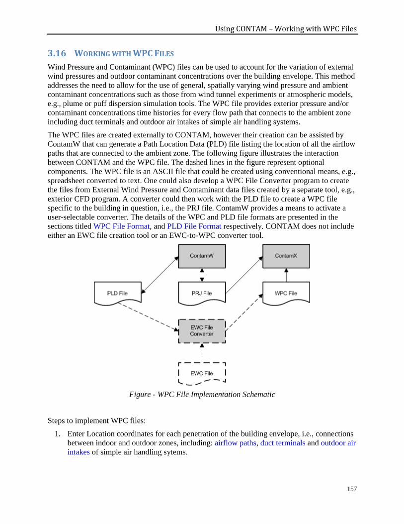
Using CONTAM – Working with WPC Files
157
3.16 WORKING WITH WPC FILES
Wind Pressure and Contaminant (WPC) files can be used to account for the variation of external
wind pressures and outdoor contaminant concentrations over the building envelope. This method
addresses the need to allow for the use of general, spatially varying wind pressure and ambient
contaminant concentrations such as those from wind tunnel experiments or atmospheric models,
e.g., plume or puff dispersion simulation tools. The WPC file provides exterior pressure and/or
contaminant concentrations time histories for every flow path that connects to the ambient zone
including duct terminals and outdoor air intakes of simple air handling systems.
The WPC files are created externally to CONTAM, however their creation can be assisted by
ContamW that can generate a Path Location Data (PLD) file listing the location of all the airflow
paths that are connected to the ambient zone. The following figure illustrates the interaction
between CONTAM and the WPC file. The dashed lines in the figure represent optional
components. The WPC file is an ASCII file that could be created using conventional means, e.g.,
spreadsheet converted to text. One could also develop a WPC File Converter program to create
the files from External Wind Pressure and Contaminant data files created by a separate tool, e.g.,
exterior CFD program. A converter could then work with the PLD file to create a WPC file
specific to the building in question, i.e., the PRJ file. ContamW provides a means to activate a
user-selectable converter. The details of the WPC and PLD file formats are presented in the
sections titled WPC File Format, and PLD File Format respectively. CONTAM does not include
either an EWC file creation tool or an EWC-to-WPC converter tool.
Figure - WPC File Implementation Schematic
Steps to implement WPC files:
1. Enter Location coordinates for each penetration of the building envelope, i.e., connections
between indoor and outdoor zones, including: airflow paths, duct terminals and outdoor air
intakes of simple air handling sytems.
Using CONTAM – Working with WPC Files
158
2. Create a WPC File according to the WPC File Format provided later in this section using
either an external editor or a user-developed EWC File Converter program.
If using an external editor, you can use the Create WPC File dialog box to generate a list
of path location data that contains the locations of all the building envelope openings. You
can also have ContamW call your EWC File Converter program via the Create WPC File
dialog box that is presented later in this section and activated via the Weather→Create
WPC File... menu command.
3. Set the simulation to utilize the WPC file (see Simultion Weather Properties in the
Working with Simulations section).
4. Verify WPC file
If you have created the WPC file using an external editor, you should verify that its
contents match that of the project file. You can do this using the View → Wind Pressure
Mode to display the WPC wind pressure type (see Checking Wind in the Defining
Weather and Wind section) or initiating the pre-simulation checks by selecting either the
Run Simulation or Create ContamX Input File from the Simulation menu.Either option
will compare the WPC and PLD files and provide notification of discrepancies between
them including location data and contaminant data that do not match. If you use and
EWC file converter program, then the verification step will occur automatically. If there
are any flow paths that do not map to a location in the WPC file, they will be highlighted
on the SketchPad and a list of these locations will be written to the CONTAMW2.LOG
file. Look for list of Paths/Terminals/Junctions not found in WPC file.
5. Run simulation
If there are errors between the WPC file and the PLD file, then ContamX will not be able
to run a simulation. ContamW will not initiate ContamX. If ContamX is run from the
command line on a project having discrepancies, it will also exit with an error message.
3.16.1 Create WPC File Dialog
The Create WPC File dialog box is a tool that can aid in the creation of WPC and associated
files.You can use this dialog box whether you are creating WPC text files using an external
editor or using an EWC File Converter. Access this dialog box via the Weather → Create WPC
File... menu item.
NOTE: WPC files can be used during a simulation in conjunction with the transient weather and
transient contaminant files as follows:
If using wind pressures from a WPC file, you may not use a WTH file.
If using contaminant concentrations from a WPC file, you may not use a CTM file.
Name of WPC File to create: This is the name of the WPC file to create using the EWC File
Converter. You can either use the Browse... button to select an existing file, or enter a new name.
WPC Description: Enter a description you want an EWC File Converter to write when creating
a new WPC file.
EWC File Name: The External Wind Pressure and Contaminant (EWC) file contains the
external contaminant concentrations and pressures that the EWC File Converter (which must be
Using CONTAM – Working with WPC Files
159
developed for your specific application) will convert into a WPC file. Use the Browse... button to
select an existing EWC file.
WPC File Creation Program: Use the Browse... button to select a program to use to create a
WPC File for example an EWC File Converter.
Coordinate Transformation Data
These parameters can be used by an EWC File Converter to establish the relationship between
the coordinates of the EWC file and the CONTAM project file. No transformation is required if
the coordinate systems for the PRJ and EWC files are consistent. These values are stored in the
PLD file by ContamW.
Origin (X, Y and Z): The location of the origin of the CONTAM PRJ file with respect to the
origin of the EWC file.
Rotation Angle: The rotation of the x and y axes of the EWC coordinate system about the z
axis to align with the x and y axes of the CONTAM coordinate system. Counter-clockwise is
considered the positive direction.
Conversion Tolerance
These are the tolerances that an EWC File Converter might use to determine how closely
information in the EWC file and the PLD file must match in order to resolve contaminant
(species) and location data. These values are stored in the PLD file by ContamW.
Species: Species can be resolved by their molar mass, i.e., the molar mass of each species
defined in ContamW and the WPC file must not differ by more than this amount to be
considered the same species.
Location: Locations can be resolved by their distance as determined by an EWC File
Converter, e.g., distance to center of a grid cell. Units within the PLD file are in meters.
Date and Time
These parameters can be used by an EWC File Converter to determine the date and time values
written to the WPC file for the convenience of working according to CONTAM's schedules.
These values are stored in the PLD file by ContamW.
Data Time Shift: The format for this value is hh:mm:ss. An EWC File Converter could add
this value to the EWC file time. For example an EWC File Converter could create a file that
begins at 00:00:00 and set the next time to be the Data Time Shift you enter here. The data
for these two times would be the initial values in the EWC file.
Start and End Date: The format for this value is mmmdd. For example, enter January 1 as
Jan01. An EWC File Converter could use this to output the date(s) to use when running
transient simulations.
Include in WPC File
Wind Pressures: Check this box to have a converter create a WPC file that contains wind
pressure data.
Contaminant Concentrations: Check this box to have the converter create a WPC file that
contains contaminant data. During a simulation contaminant concentrations in the WPC file
take precedence over other transient contaminant settings. For those contaminants that are
Using CONTAM – Working with WPC Files
160
defined within the PRJ file but not included in the WPC file, the steady-state contaminant
data will be used, i.e., the default concentrations.
Generate WPC File: Use this button to activate the user-developed WPC Creation Program.
This will first perform checks on the PRJ file and generate a PLD file if all envelope openings
are properly defined.
Generate PLD File: Use this button to manually generate a PLD file. The PLD file will be
stored in the same location as the PRJ file and have the same name as the PRJ file but a PLD
extension. This file is useful for creating a WPC file with an external editor.
3.16.2 Envelope Opening Locations
When using WPC Files you must enter the coordinates for each opening connected to the
ambient including: airflow paths, duct terminals, and outdoor air intakes of simple air handling
systems. Coordinate data is input via the Wind Pressure Property Pages of these building
components. The location information will be used to create the PLD File which in turn is used
to verify that there is matching information within the WPC File prior to performing a
simulation.
NOTE: Even though every opening connected to ambient requires location data when using
WPC Files, they are not required to be unique. They simply must match a location within the
WPC File.
Airflow Paths and Duct Terminals Enter the X and Y coordinates and units for each airflow path and duct terminal. The Z
coordinate will be calculated by ContamW to be the Relative Elevation plus the Elevation of the
building level on which the path or terminal is located.
Outdoor Air Intakes of Simple Air Handling Systems Enter the X, Y and Z coordinates and units for the outdoor air intake of each Simple AHS. Enter
the Z coordinate as the height of the midpoint of the outdoor air intake with respect to the
building reference height.
3.16.3 WPC File Format
This file provides ambient pressure and contaminant concentrations values for every flow path
that connects to ambient.
There are two versions of the WPC file 2.1 and 2.4. For version 2.1, pressures must be input as
absolute pressures in units of Pa. Wind pressure will be computed from the ambient pressure and
density provided at each time interval in the WPC file and the absolute pressure and elevation of
each flow path as follows:
Pwind = Ppath - Pambt + •g•Zpath
For 2.4 version files the pressure in the WPC file will be the wind pressure itself in units of Pa.
Contaminant concentrations must be provided in units of kg of contaminant per kg of air. See
Concentration Conversions in the Contaminant Files subsection of the Working with Species and
Contaminants section for conversion factors.
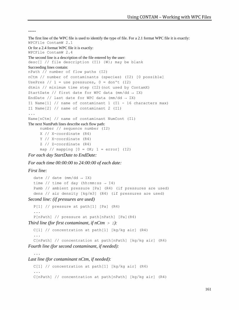
Using CONTAM – Working with WPC Files
161
-----
The first line of the WPC file is used to identify the type of file. For a 2.1 format WPC file it is exactly: WPCFile ContamW 2.1
Or for a 2.4 format WPC file it is exactly: WPCFile ContamW 2.4
The second line is a description of the file entered by the user: desc[] // file description (I1) {W}; may be blank
Succeeding lines contain: nPath // number of flow paths (I2)
nCtm // number of contaminants (species) (I2) [0 possible]
UsePres // 1 = use pressures, 0 = don't (I2)
dtmin // minimum time step (I2)(not used by ContamX)
StartDate // first date for WPC data (mm/dd → IX)
EndDate // last date for WPC data (mm/dd → IX)
I1 Name[1] // name of contaminant 1 (I1 - 16 characters max)
I1 Name[2] // name of contaminant 2 (I1)
...
Name[nCtm] // name of contaminant NumCont (I1)
The next NumPath lines describe each flow path: number // sequence number (I2)
X // X-coordinate (R4)
Y // X-coordinate (R4)
Z // Z-coordinate (R4)
map // mapping [0 = OK; 1 = error] (I2)
For each day StartDate to EndDate:
For each time 00:00:00 to 24:00:00 of each date:
First line:
date // date (mm/dd → IX)
time // time of day (hh:mm:ss → I4)
Pamb // ambient pressure [Pa] (R4) (if pressures are used)
dens // air density [kg/m3] (R4) (if pressures are used)
Second line: (if pressures are used)
P[1] // pressure at path[1] [Pa] (R4)
...
P[nPath] // pressure at path[nPath] [Pa](R4)
Third line (for first contaminant, if nCtm > 1):
C[1] // concentration at path[1] [kg/kg air] (R4)
...
C[nPath] // concentration at path[nPath] [kg/kg air] (R4)
Fourth line (for second contaminant, if needed):
...
Last line (for contaminant nCtm, if needed):
C[1] // concentration at path[1] [kg/kg air] (R4)
...
C[nPath] // concentration at path[nPath] [kg/kg air] (R4)
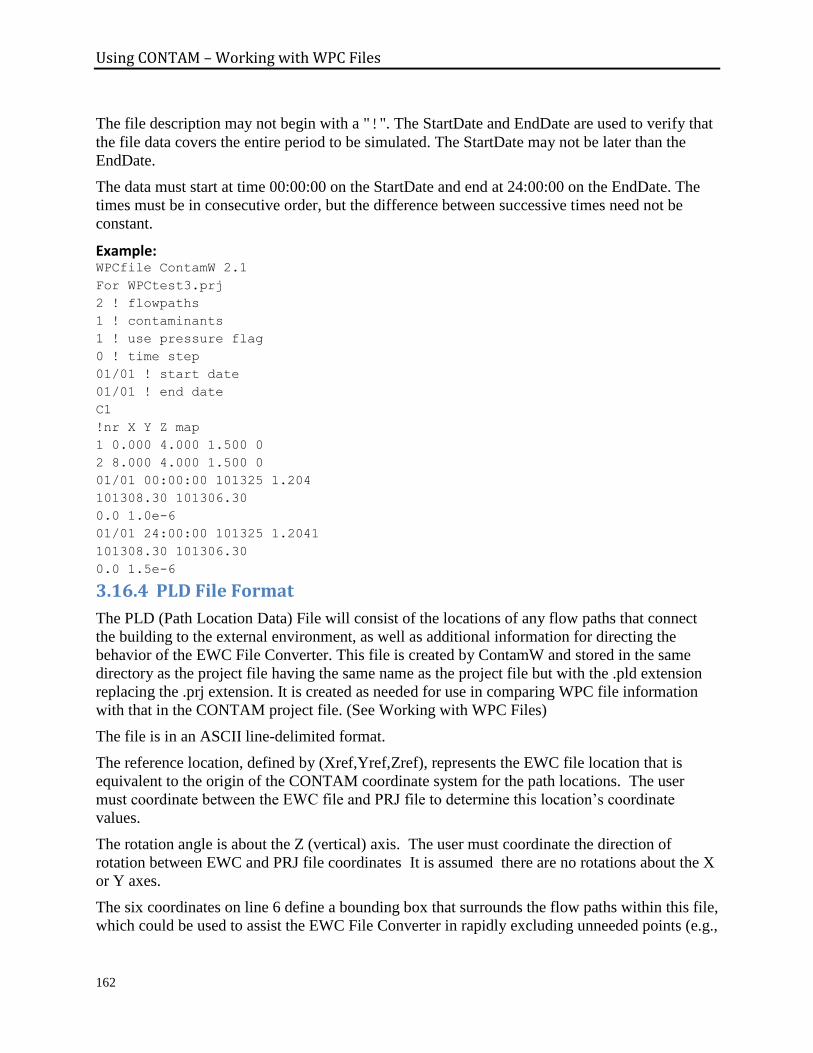
Using CONTAM – Working with WPC Files
162
The file description may not begin with a "!". The StartDate and EndDate are used to verify that
the file data covers the entire period to be simulated. The StartDate may not be later than the
EndDate.
The data must start at time 00:00:00 on the StartDate and end at 24:00:00 on the EndDate. The
times must be in consecutive order, but the difference between successive times need not be
constant.
Example: WPCfile ContamW 2.1
For WPCtest3.prj
2 ! flowpaths
1 ! contaminants
1 ! use pressure flag
0 ! time step
01/01 ! start date
01/01 ! end date
C1
!nr X Y Z map
1 0.000 4.000 1.500 0
2 8.000 4.000 1.500 0
01/01 00:00:00 101325 1.204
101308.30 101306.30
0.0 1.0e-6
01/01 24:00:00 101325 1.2041
101308.30 101306.30
0.0 1.5e-6
3.16.4 PLD File Format
The PLD (Path Location Data) File will consist of the locations of any flow paths that connect
the building to the external environment, as well as additional information for directing the
behavior of the EWC File Converter. This file is created by ContamW and stored in the same
directory as the project file having the same name as the project file but with the .pld extension
replacing the .prj extension. It is created as needed for use in comparing WPC file information
with that in the CONTAM project file. (See Working with WPC Files)
The file is in an ASCII line-delimited format.
The reference location, defined by (Xref,Yref,Zref), represents the EWC file location that is
equivalent to the origin of the CONTAM coordinate system for the path locations. The user
must coordinate between the EWC file and PRJ file to determine this location’s coordinate
values.
The rotation angle is about the Z (vertical) axis. The user must coordinate the direction of
rotation between EWC and PRJ file coordinates It is assumed there are no rotations about the X
or Y axes.
The six coordinates on line 6 define a bounding box that surrounds the flow paths within this file,
which could be used to assist the EWC File Converter in rapidly excluding unneeded points (e.g.,

Using CONTAM – Working with WPC Files
163
that are too distant from the building) during the mapping process. Note that this bounding box
does not necessarily surround the entire building.
The simulation time step provides a recommendation to the EWC File Converter for reducing the
size of the WPC file, so that only the time steps that coincide with the simulation time step could
be included (which could reduce interpolation required).
Each flow path is uniquely identified by a combination of flow path type and flow path ID
values.
Comments begin with an exclamation point (’!’) and may begin at the start of any line (so that
the entire line will be ignored) or after all fields of a line (so that the remainder of the line will be
ignored).
For user readability, fields should be commented whenever possible.
The format of R4 data types may be interpreted similar to a C scanf() statement’s conversion
specification.
Header Section:
First three lines:
EWC filename // (I1 full path)
WPC filename // (I1 full path)
desc[] // file description (I1)
The next header line is exactly:
! Xref Xref Yref angle
The next line contains reference coordinates in meters:
Xref // (R4 %7.3f)
Yref // (R4 %7.3f)
Zref // (R4 %7.3f)
rotation angle // Real format %8.3f
The next line contains latitude and longitude in units of degrees:
latitude // (R4 %8.4f) positive for North
longitude // (R4 %8.4f) positive for East
The next bounding box header line is exactly:
! Xmin Xmax Ymin Ymax Zmin Zmax
The next line contains bounding box coordinates:
Xmin // (R4 %7.3f)
Xmax // (R4 %7.3f)
Ymin // (R4 %7.3f)
Ymax // (R4 %7.3f)
Zmin // (R4 %7.3f)
Zmax // (R4 %7.3f)
The next time step heading line is exactly:
! step shift start end
The next line contains time step data:
time step // (I4) [s]
data shift // (hh:mm:ss → I4) start time for EWC when converted to WPC
start date // (mm/dd → IX)
end date // (mm/dd → IX)
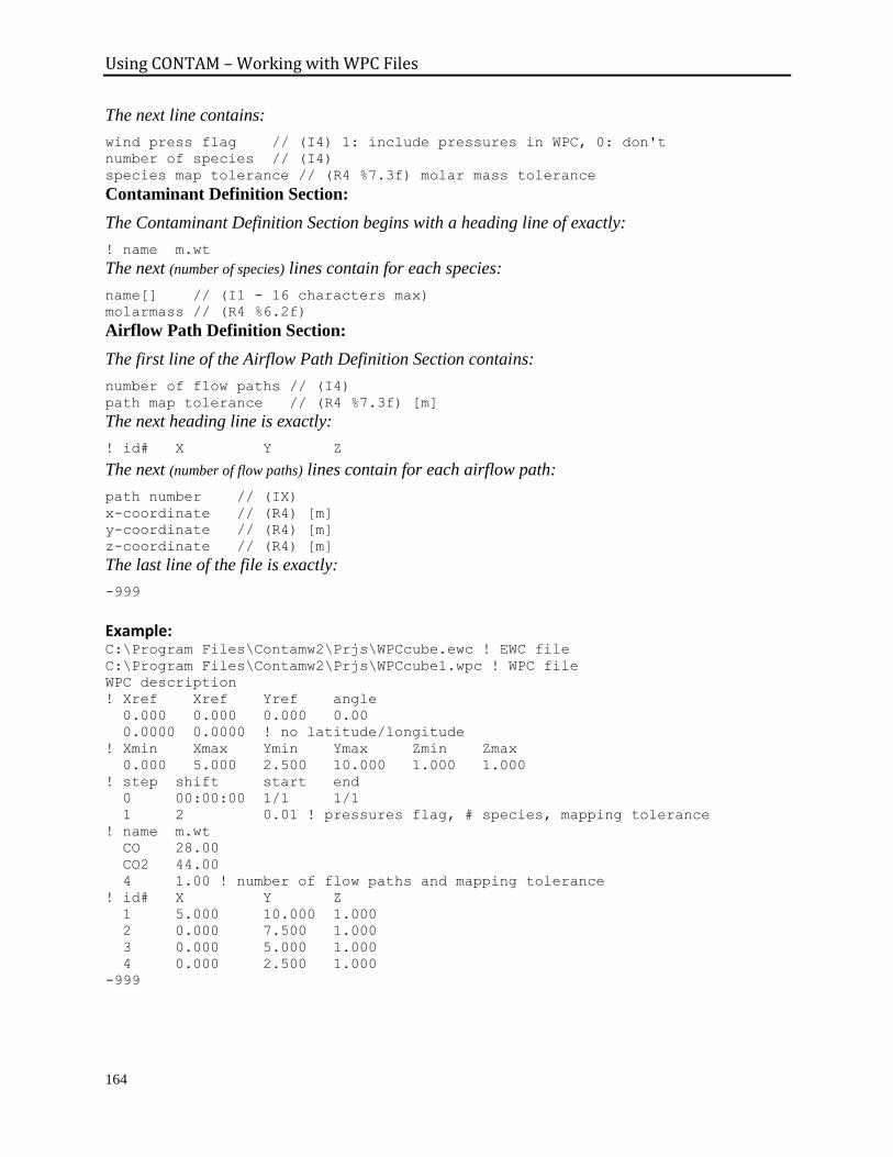
Using CONTAM – Working with WPC Files
164
The next line contains:
wind press flag // (I4) 1: include pressures in WPC, 0: don't
number of species // (I4)
species map tolerance // (R4 %7.3f) molar mass tolerance
Contaminant Definition Section:
The Contaminant Definition Section begins with a heading line of exactly:
! name m.wt
The next (number of species) lines contain for each species:
name[] // (I1 - 16 characters max)
molarmass // (R4 %6.2f)
Airflow Path Definition Section:
The first line of the Airflow Path Definition Section contains:
number of flow paths // (I4)
path map tolerance // (R4 %7.3f) [m]
The next heading line is exactly:
! id# X Y Z
The next (number of flow paths) lines contain for each airflow path:
path number // (IX)
x-coordinate // (R4) [m]
y-coordinate // (R4) [m]
z-coordinate // (R4) [m]
The last line of the file is exactly:
-999
Example: C:\Program Files\Contamw2\Prjs\WPCcube.ewc ! EWC file
C:\Program Files\Contamw2\Prjs\WPCcube1.wpc ! WPC file
WPC description
! Xref Xref Yref angle
0.000 0.000 0.000 0.00
0.0000 0.0000 ! no latitude/longitude
! Xmin Xmax Ymin Ymax Zmin Zmax
0.000 5.000 2.500 10.000 1.000 1.000
! step shift start end
0 00:00:00 1/1 1/1
1 2 0.01 ! pressures flag, # species, mapping tolerance
! name m.wt
CO 28.00
CO2 44.00
4 1.00 ! number of flow paths and mapping tolerance
! id# X Y Z
1 5.000 10.000 1.000
2 0.000 7.500 1.000
3 0.000 5.000 1.000
4 0.000 2.500 1.000
-999
Using CONTAM – Working with Schedules
165
3.17 WORKING WITH SCHEDULES
Schedules provide you with the ability to modify various parameters based on the time of day
and day of the week. You use schedules to set or modify values of controlled parameters at times
which you define. You can schedule parameters such as the flow through airflow paths; ducts;
simple air handling system inlets, outlets and fraction of outdoor air intake; contaminant
source/sinks; the location and contaminant generation rate of occupants; and zone temperatures.
CONTAM provides occupant schedules and non-occupant schedules which are split up into
week schedules which are in turn made up of one or more day schedules. Non-occupant week
schedules can be associated with as many schedulable items as you need, whereas occupant
week schedules can only be applied to a single occupant. Only non-occupant schedules can be
shared between CONTAM project files using the ContamW Library Manager. Occupant
schedules can not be shared between projects, because they are dependent on the level and zone
names which may be different between projects. The following sections provide detailed
information related to the creation, modification and deletion of schedules in ContamW.
Schedules apply when performing both transient and steady-state simulations, and schedule
values are accessed according to the Day Type and time during a simulation. The Day Type is
used to select one of twelve day schedules that make up each week schedule as explained below.
The Day Type will be determined during simulation via either the steady state or transient
weather data (See Run Control Properties in the Working with Simulations section). For greater
scheduling flexibility, use the CVF and DVF control types which allow scheduling to vary over
the course of a year (see CVF/DVF in the Working with Controls section).
If a schedule and a control signal (see Working with Controls) are both associated with the same
building element icon, then the control signal will take precedence over the schedule during
simulation.
3.17.1 Creating Schedules
You can create schedules using either the CONTAMW Library Manager (see Working with Data
and Libraries) or wherever a "New Schedule" button is provided when working with various
building component property sheets (e.g. airflow paths, ducts, source/sinks, and occupant icons).
Non-occupancy Schedules You create non-occupant schedules by first selecting to create a new week schedule to display
the Week Schedule dialog box. You must then define one or more day schedules that you then
associate with each day of the week schedule. Each week schedule consists of 12 days – one for
each day of the week and five more days that you can use for special situations such as holidays.
These are refered to as the 12 day types. New day schedules are created from the Week Schedule
dialog box by clicking on the "New Schedule" button. This will display the Day Schedule dialog
box whose features are explained below.
Temperature Schedules Temperature schedules are a type of non-occupant schedule. Unlike other non-occupant
schedules they have units associated with them. Temperature schedules are only associated with
zones and duct junctions and are considered separately from other non-occupant schedules when
creating and editing. For instance, when displaying a list of temperature schedules, only those

Using CONTAM – Working with Schedules
166
non-occupancy schedules having temperature units will be displayed (unitless schedules will not
be displayed).
Occupancy Schedules You create occupant schedules by first creating an occupant exposure icon (see Creating
Occupants). You then click on the "Edit Occupancy Schedule" button that is provided on the
Occupant Data property page of the "Occupant Exposure Properties" property sheet.
3.17.2 Modifying Schedules
You modify existing non-occupancy week and day schedules through the Week Schedule and
Day Schedule dialog boxes respectively. Edit occupancy schedules by editing the properties of
existing occupant exposure icons. The details of editing schedules are presented in the following
sections.
3.17.3 Deleting Schedules
You can only delete occupancy week schedules by deleting the associated occupant exposure
icon. Deleting all other schedules can only be accomplished using the CONTAMW Library
Manager (see Working with Data and Libraries) which will only allow you to delete those
schedules that are no longer associated with any occupants, zones or other building components.
3.17.4 Week Schedule Properties
These are the properties and methods you use to define non-occupancy week schedules. You
must associate a day schedule with each day of a week schedule (7 days of the week plus 5 extra
days). The extra days are provided for any day that may have a non typical schedule, such as a
holiday. Once defined, you may display the schedule graphically by pressing the "Display
Graphically" button.
Name: This is the name you give to this week schedule. This name must be unique among the
week schedules within this project.
Units: Select the temperature units to use when defining a zone temperature schedule. This
control will only be available if these properties are accessed from a zone property sheet, Zone
Data or via the Data → Week SchedulesTemperature… menu selection.
Description: Field for entering a more detailed description of the specific schedule.
Day Schedules: Every "Week Schedule" consists of twelve days (day type 1 - 12) that must be
associated with "Day Schedules". These day schedules may or may not be unique for each of the
12 days. If the project has no available day schedules a new day schedule must be defined. Do
this by pressing the "New Day Schedule" button, then editing the day schedule as explained in
the section entitled "Day Schedule." You can edit existing day schedules by selecting them in the
"Available Schedules" list box and then pressing the "Edit Day Schedule" button, then following
the procedure explained in the Day Schedule section. If a day has already been associated with a
day schedule you can change it by first highlighting the day to be changed in the Day Schedules
list box, highlighting the day schedule to replace the existing schedule, and then pressing the "<<
Replace <<" button.
Only those day schedules of the same type as the week schedule will appear in the list of day
schedules, i.e., dimensionless or temperature.
Using CONTAM – Working with Schedules
167
3.17.5 Day Schedule Properties
These are the properties and methods you use to define day schedules. You may display the
schedule graphically by pressing the "Display Graphically" button.
Name: This is the name you give to this day schedule. This name must be unique among the day
schedules within a project.
Description: Field for entering a more detailed description of the specific schedule.
Shape: Use this check box to set how CONTAMW interprets values between the data points you
define.
Rectangular: characterized by a step function between the data points
Trapezoidal: characterized by linear interpolation between the data points.
Schedule Data: These are the time/multiplier pairs that you set to define a day schedule. The
times are entered in the hh:mm:ss format.
For unitless schedules, the value is a multiplier between 0.0 and 1.0 used to adjust down the
maximum design values of various schedulable building components, e.g., constant volume flow
rate of a fan flow element.
To insert a new data point Enter the new time/multiplier pair in the "Time" and "Value" edit boxes in the Edit Schedule
Value Section of the dialog box and press the "<< Insert <<" button. The data point will be
inserted into the schedule in the correct sequence.
To modify an existing data point Select the data point that you wish to modify from the list, enter the revised data, and press the
"<< Insert <<" button to overwrite the previously entered data point.
To delete an existing data point Select the data point you want to delete from the list and click the "Delete" button. You can not
delete 00:00:00 or 24:00:00.
3.17.6 Occupant Week Schedule Properties
These are the properties and methods you use to define occupant week schedules.
Description: Field for entering a more detailed description of the specific schedule.
Day Schedules: Every "Occupancy Week Schedule" consists of twelve days (12 day types) that
must be associated with Occupant Day Schedules. These schedules may or may not be unique
for each of the twelve day types. If the project has no available day schedules a new day
schedule must be defined. This is done by pressing the "New Day Schedule" button then editing
the day schedule as explained in the Occupant Day Schedule section. You may edit existing day
schedules by selecting them in the "Available Schedules" list box, pressing the "Edit Schedule"
button, and then following the procedure explained in the Occupant Day Schedule section. If a
day has already been associated with a day schedule, you may changed it by first highlighting the
day to be changed in the Day Schedules list box, then highlighting the day schedule to replace
the existing schedule, and finally pressing the "<< Replace <<" button.

Using CONTAM – Working with Schedules
168
3.17.7 Occupant Day Schedule Properties
These are the properties and methods you use to define occupant day schedules.
Name: This is the name you give to this occupant day schedule. This name must be unique
among the occupant day schedules within this project.
Description: Field for entering a more detailed description of the specific schedule.
Schedule Data: These are the time/location data points that you set to define an occupancy day
schedule. The times are entered in the hh:mm:ss format, and you must provide leading and
trailing zeros; for example 9:30 am would be entered as 09:30:00 not as 9:30:00. The location
consists of a level and zone in which the occupant resides for the indicated time period. Select a
value of "null" from the zone list to indicate the occupant is not in the building for a given time
period.
Location data will also include zone coordinates if the occupant enters a 1D convection diffusion
zone. For such cases, enter the X, Y and Relative Elevation (Z) coordinates and units for each 1D
zone the occupant enters. X and Y are absolute coordinates and Rel Elevation is relative to the
level of each1D zone that the occupant enters.
To insert a new data point Enter the new time and location data in the "Modify Data" block, press the "<< Insert <<" button
and the data point will be inserted into the schedule in the correct sequence.
To modify an existing data point Select the data point that you wish to modify from the list, enter the revised data, and press the
"<< Insert <<" button to overwrite the previously entered data point.
To delete an existing data point Select the data point you want to delete from the list and click the "Delete" button. You can not
delete 00:00:00 or 24:00:00.
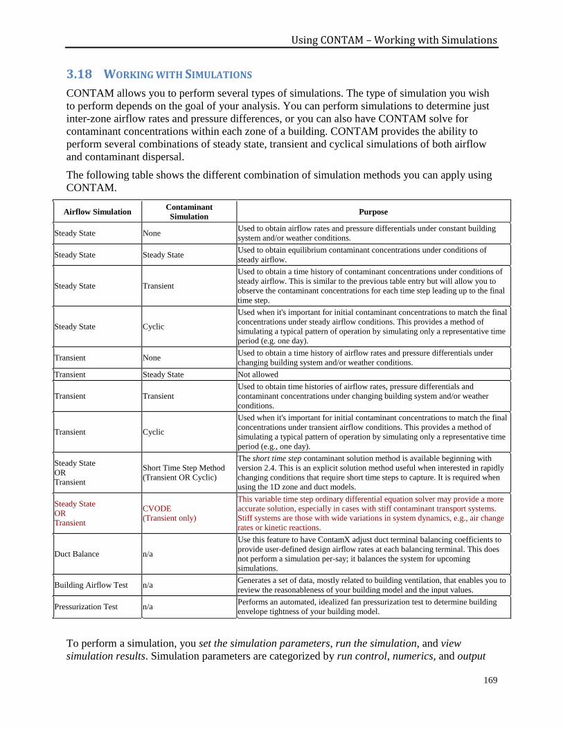
Using CONTAM – Working with Simulations
169
3.18 WORKING WITH SIMULATIONS
CONTAM allows you to perform several types of simulations. The type of simulation you wish
to perform depends on the goal of your analysis. You can perform simulations to determine just
inter-zone airflow rates and pressure differences, or you can also have CONTAM solve for
contaminant concentrations within each zone of a building. CONTAM provides the ability to
perform several combinations of steady state, transient and cyclical simulations of both airflow
and contaminant dispersal.
The following table shows the different combination of simulation methods you can apply using
CONTAM.
Airflow Simulation Contaminant
Simulation Purpose
Steady State None Used to obtain airflow rates and pressure differentials under constant building
system and/or weather conditions.
Steady State Steady State Used to obtain equilibrium contaminant concentrations under conditions of
steady airflow.
Steady State Transient
Used to obtain a time history of contaminant concentrations under conditions of
steady airflow. This is similar to the previous table entry but will allow you to
observe the contaminant concentrations for each time step leading up to the final
time step.
Steady State Cyclic
Used when it's important for initial contaminant concentrations to match the final
concentrations under steady airflow conditions. This provides a method of
simulating a typical pattern of operation by simulating only a representative time
period (e.g. one day).
Transient None Used to obtain a time history of airflow rates and pressure differentials under
changing building system and/or weather conditions.
Transient Steady State Not allowed
Transient Transient
Used to obtain time histories of airflow rates, pressure differentials and
contaminant concentrations under changing building system and/or weather
conditions.
Transient Cyclic
Used when it's important for initial contaminant concentrations to match the final
concentrations under transient airflow conditions. This provides a method of
simulating a typical pattern of operation by simulating only a representative time
period (e.g., one day).
Steady State
OR
Transient
Short Time Step Method
(Transient OR Cyclic)
The short time step contaminant solution method is available beginning with
version 2.4. This is an explicit solution method useful when interested in rapidly
changing conditions that require short time steps to capture. It is required when
using the 1D zone and duct models.
Steady State
OR
Transient
CVODE
(Transient only)
This variable time step ordinary differential equation solver may provide a more
accurate solution, especially in cases with stiff contaminant transport systems.
Stiff systems are those with wide variations in system dynamics, e.g., air change
rates or kinetic reactions.
Duct Balance n/a
Use this feature to have ContamX adjust duct terminal balancing coefficients to
provide user-defined design airflow rates at each balancing terminal. This does
not perform a simulation per-say; it balances the system for upcoming
simulations.
Building Airflow Test n/a Generates a set of data, mostly related to building ventilation, that enables you to
review the reasonableness of your building model and the input values.
Pressurization Test n/a Performs an automated, idealized fan pressurization test to determine building
envelope tightness of your building model.
To perform a simulation, you set the simulation parameters, run the simulation, and view
simulation results. Simulation parameters are categorized by run control, numerics, and output
Using CONTAM – Working with Simulations
170
properties. Run control properties include the simulation methods, simulation dates and times,
type of weather to use (steady or transient), and simulation time step. Output properties are used
to set the type and amount of data you wish to have sent to the simulation results files. Numerics
properties include convergence criteria, maximum iterations and relaxation coefficients for both
airflow and contaminant equation solvers. ContamW provides default settings for these
parameters. However, you will probably work more with the run control and output parameters
than the numerics parameters.
Setting Simulation Parameters To set simulation parameters you use the Set Simulation Parameters… selection of the
Simulation menu or the F4 keyboard shortcut. This will display the "Simulation Parameters"
property sheet. Detailed descriptions of all simulation properties are given in the Simulation
Parameters section of this documentation.
Running Simulations via ContamW Once you have set the simulation parameters, you can run the simulation. To run a simulation
select Run Simulation from the Simulation menu. This actually launches a separate program,
ContamX, which in turn displays the "CONTAMX Simulation Control" dialog box.
While there are many factors that can affect the ability of ContamX to quickly and successfully
obtain a solution (converge), there are situations that can cause the simulation to not converge or
to converge very slowly. The relative magnitudes of the flow coefficients have some effect on
the convergence of the nonlinear equation solver of ContamX [Wray and Yuill 1993]. Airflow
networks containing paths whose resistances differ by many orders of magnitude will typically
require more iterations than networks with paths of similar resistances. Reducing the relaxation
coefficient from its default value of 0.75 to a value nearer one-half can often help convergence of
these more difficult cases. The maximum number of iterations can also be increased. However,
the most effective way to improve convergence is to remove those very low resistance paths that
are not likely to effect the computed airflow rates. For example, when simulating a shaft (see
Shafts), represent a shaft using phantom zones as opposed to using airflow elements with large
cross-sectional areas between zones on adjacent levels.
Running Simulations via Command Line CONTAM utilizes the ContamX stand-alone simulation engine, contamx3.exe. ContamX utilizes
the same .PRJ file that you create using ContamW. With the ContamX program, you can perform
batch mode operations to process multiple project files. Or you can create your own file
processor to modify project files, for example to perform sensitivity analysis by performing
multiple runs while varying desired building parameters. If you wish to modify the .PRJ file in
such a manner, you should become familiar with the .PRJ file format that is now annotated with
comment lines to improve the legibility of the file. (see Appendix A - PRJ File Format)
To obtain a PRJ file for command-line use, you can simply create and save the project in the
usual manner using ContamW. To check that the project is “well formed”, you can either use
ContamW to run a simulation with the file, or use the Run Building Check selection of the
Simulation menu. This is especially important if new controls have been added to the project,
because ContamW must determine the proper evaluation sequence of the controls. Sequence
values will be saved to the project file for each control.
Using CONTAM – Working with Simulations
171
Building Check Note this building check is also performed prior to initiating a simulation from within ContamW
via the Simulation → Run Simulation menu command. If during the building check routine
ContamW detects problems with your project, it will provide you with feedback to assist you in
correcting the problems. This feedback will be provided by displaying the Building Check
dialog box which will display a list problems found and allow you to highlight problematic icons
on the SketchPad as necessary.
Viewing Simulation Results Once you have successfully run a simulation, you can use ContamW to view simulation results
or to create files that can be imported into a spreadsheet. These capabilities are explained in the
Working with Results section.
3.18.1 CONTAMX Simulation Control
The "ContamX Simulation Control" dialog box allows you to control and view the status of a
simulation. Once you have set the simulation parameters, activate the CONTAMX Simulation
Control dialog via the Simulation Run Simulation command from the ContamW menu.
Press the "Start Simulation" button to run the simulation. If at any point during the simulation
you want to terminate the simulation, press the "Stop Simulation" button.
Simulation Status: The current status of the simulation is displayed in this section. The date,
time, day, and the current iteration of the simulation are shown. A check box is provided to
terminate cyclic simulations at the end of the next cycle/day. Use this check box if it appears the
simulation is not converging, or you feel enough iterations have been performed.
Simulation Settings: This field displays a summary of the current Run Control simulation
parameters. This is provided for convenience to enable you to review the type of simulation that
CONTAM is currently configured to perform.
Start Simulation: Press this button to start a simulation. Once you start a simulation, any
existing results files for the current project file will be deleted. If you wish to save the current
result files, you should either rename the files, move them to a location other than the directory
in which the project file exists, or rename the current project file so that new results files are
created associated with the new name.
Stop Simulation: Press this button to immediately terminate a simulation.
3.18.2 Simulation Parameters
Simulation parameters are those used to control the type of simulation that you wish ContamX to
perform and the type of results output you wish ContamX to provide. This section provides
detailed descriptions of the specific simulation parameters.
Simulation – Run Control Properties
Simulation Method Set the type of simulation you wish to perform for both Airflows and Contaminants by checking
the appropriate radio buttons. Refer to the Working with Simulations section for a table of
allowable combinations of simulation method settings.
Airflows: You can use one of the following airflow calculation methods.

Using CONTAM – Working with Simulations
172
Steady: A steady state simulation will utilize the weather set by pressing the Edit Weather
Button on the Run Control property page. This will calculate a single set of airflows. If any
building components have schedules associated with them, then schedule values will be
determined by the Day Type set in the Steady State Weather Data (see Weather Properties
under Working with Weather and Wind) and the Steady Simulation Time.
Transient: Transient simulations perform calculations over a user-defined period of time
at a regular time interval referred to as the calculation time step. When performing a
transient simulation CONTAM can use either steady state weather data or weather and
contaminant files that define the weather and ambient contaminant concentrations for the
time period of the simulation. See Defining Transient Weather and Wind in the Working
with Weather and Wind section for more details.
Duct Balance: Use this feature when working with detailed duct systems to have
CONTAM adjust terminal duct balancing coefficients to provide user-defined airflow rates
at the duct terminals. See Working with Ducts.
Building Airflow Test: The building airflow test method performs calculations that aid in
verifying data input to your building model. Use this test prior to performing analysis with
your building model to verify system and total airflow rates to each zone, zone
temperatures and whole building air change rate. You must have only one contaminant set
to be used in the simulation, and it must be a trace contaminant, when you run this test.
Results of the test will be written to the validation file having the same name as the project
file and the .val extension (see Working with Results). This file will be overwritten each
time either the Building Airflow Test or Building Pressurization Test is performed.
Building Pressurization Test: The building pressurization method performs an automated
whole-building fan pressurization test (see Special Applications of CONTAM) to
determine building envelope airtightness under idealized test conditions. See the Special
Applications of CONTAM section for a detailed discussion of building pressurization
tests.
ContamX will temporarily set conditions for the duration of the building pressurization
calculation as follows:
o no-wind
o ambient pressure set to steady state barometric pressure
o ambient and interior zones set to 20 ºC
o conditioned zones (included in building volume) set to constant test pressure
NOTE: This will eliminate the effect of airflow between building zones as explained
in the Special Applications of CONTAM section.
o unconditioned zones (not included in building volume) set to variable pressure
o “close” all duct terminals and duct leaks
o “turn off” all forced flow elements
When you perform a simulation using this method, ContamX will perform a steady
state airflow calculation under the above conditions and calculate the total airflow
rate between conditioned and unconditioned zones of the project. Results of the test
Using CONTAM – Working with Simulations
173
will be written to the validation file having the same name as the project file and the
.val extension (see Working with Results). This file will be overwritten each time
either the Building Airflow Test or Building Pressurization Test is performed.
Contaminants: You can choose one of the following contaminant simulation options:
None: Do not perform contaminant analysis, only airflow analysis.
Steady: The steady contaminant option can only be used in conjunction with steady
airflows and will run until the system reaches equilibrium. Contaminant sources are
modeled as continuous sources with a constant generation rate. If any sources have
schedules associated with them, then schedule values will be determined by the Day Type
set in the Steady State Weather Data (see Weather Properties under Working with Weather
and Wind) and the Steady Simulation Time. Burst sources will be ignored. Ambient
contaminant concentrations will be the Default Concentration values of each contaminant.
Transient: Transient simulations performs calculations over a user-defined period of time
and at a regular time interval referred to as the calculation time step. When performing a
transient simulation CONTAM can use either constant ambient concentrations as given by
default contaminant concentrations or dynamic concentrations from external contaminant
files. See Contaminant Files and Working with WPC Files.
Cyclic: A cyclic simulation repeats a 24h cycle until steady-periodic conditions are
achieved. As with transient simulations, cyclic simulations can implement either steady
state or dynamic weather and contaminant data. If using dynamic weather or contaminant
data files (CTM and WTH), data will be obtained from the file for the date indicated by
Steady & Cyclic Simulations date.
Transient Integration Method: Select the type of transient or cyclic simulation to perform from
the available options. More detailed options are available via the Contaminant Numerics
simulation parameters.
Default Solver (Implicit Euler): This is the traditional, fixed time step solver.
Short Time Step (Explicit Euler): You can use this method with either the Transient or
Cyclic contaminant simulation methods. This method is required to perform simulations of
one-dimensional convection diffusion zones and/or ducts. See Contaminant Numerics
Properties for specific control in applying the short time step method to 1D ducts and 1D
zones.
NOTE: This is an explicit solution method that should only be used for short time steps,
therefore there are some checks performed to help avoid known stability problems.
ContamX will check the zone airflow rates (of all zones having non-zero volumes) during
airflow simulation to ensure that they do not exceed one air change per time step. If this
limitation is exceeded for any zone, then the simulation will be terminated with an error
message indicating the offending zone(s). The problem could also manifest itself with an
error message indicating an invalid zone density was calculated due to the calculation of a
negative absolute pressure.
CVODE: This is a variable time step ordinary differential equation solver [Hindmarsh and
Serban 2012]. It may provide a more accurate solution, especially in cases with stiff
contaminant transport systems. Stiff systems are those with wide variations in system
Using CONTAM – Working with Simulations
174
dynamics, e.g., air change rates or kinetic reactions [Lorenzetti 2013].
NOTE: This solver is currently limited in that it will not handle projects that contain 1D
zones, CFD zones, occupant exposure, burst sources, or zones (nodes) with zero volume.
Further, the CVODE solver does not support the bridge mode (socket communication
capabilities).
Reset initial contaminant concentrations to…: Use this feature to reset the initial contaminant
concentrations of all zones, including the implicit supply and return zones of simple air handling
systems, prior to running a simulation. You can reset initial concentrations to Zero, Ambient or
Current Results Concentrations. If you do not check one of these boxes, ContamX uses the
Initial Concentrations indicated on the Contaminant Property page for each zone (See
Contaminant Data under the Working with Zones section). Checking one of these boxes causes
the Initial Concentration values for each zone to be overwritten.
Zero: This option sets the initial contaminant concentrations to zero.
Ambient Concentrations: This option sets the initial contaminant concentrations to the
default contaminant concentrations as set when defining Project Species (See Species
Properties).
Current Results Concentrations: This option sets the initial contaminant concentrations
to be the same as the concentrations in each zone at the time step for which ContamW is
currently displaying results on the SketchPad. You must be in the results viewing mode to
utilize this feature. The current time step is displayed in the middle pane of the Status Bar
(See the Status Bar section). This option is especially useful for cyclic simulation, where
you may continue a simulation that has been interrupted before convergence, continue
simulation with tighter convergence criteria, or create a project file for archive which can
be rerun as a one-day transient simulation to quickly compute cyclic results.
Simulation Dates and Times These dates and times are used to set the date and time labels put on steady state simulation
results and to control the duration of transient simulations by allowing you to set the start and
stop dates and times. Depending on the simulation method chosen different simulation "Dates
and Times" fields will be enabled or disabled.
Steady & Cyclic Simulations: For steady simulations, the date field is only used to label
the simulation results, however, the time field is used to obtain schedule values from the
day schedules based on the day type which the simulation is set to utilize. You set the Day
Type via the steady state Weather and Wind Parameters property sheet (see Weather
Properties under Working with Weather and Wind). ContamX will then utilize the Day
Type and time to select schedule values for items that have schedules associated with
them. The value of Day Type will be from 1 to 12 and will be used to select from the
twelve day schedules associated with each week schedule in use during a simulation.
For cyclic simulations with steady airflows, the date field is only used to label the
simulation results, and the day type of the steady state data is used to determine schedule
values. For cyclic simulation with transient airflows, the date field is used to determine
schedule values and obtain data from weather and contaminant files if being used,
otherwise steady state data is used. Cyclic simulations always begin at time 00:00:00 and
end at time 24:00:00, so the time field is irrelevant.
Using CONTAM – Working with Simulations
175
Transient Simulation, Start and Stop: These date and time fields are used to set the
starting and stopping date and time of transient simulations. You should be sure to use
only those dates available in both the weather and ambient contaminant files. The available
dates in these files will be displayed in the Transient Weather Data and Transient
Contaminant Data sections below. Each day of the WTH file contains a Day Type field
which will be used to determine which of each week schedule's twelve day schedules
should be used for each day of simulation.
NOTE: If using steady state weather with a transient simulation, simulation will begin with
the Day Type set in the steady state weather and cycle through the first seven day
schedules if simulating more than one day.
Use restart file: Each transient and cyclic simulation produces a restart file that contains
the status of the simulation at midnight for each day of the simulation, and at the last time
step of a simulation if it does not end at midnight. The restart file will have the same name
as the PRJ file but have the RST extension. If a restart file with the same name as the
project file is available, the dates for which restart data is available will be listed as
"Restart data from ___ to ___" below the "Use restart file" check box. Enter the date in the
edit box labeled “Restart data beginning.” If a restart file is used in a simulation, the
existing restart file will be overwritten.
This feature can be useful when running long multi-day simulations with the potential for
generating impractically large detailed simulation results files. You can avoid the
generation of large results files by running the multi-day simulation outputting only
summary data files, reviewing the results to determine days of interest, e.g., highest
concentration, then rerunning the simulation for the days of interest using the restart file
and outputting detailed results.
You can also use this feature to load boundary layer and deposition/resuspension
source/sinks by first running a cyclic simulation for a single day, then using the restart file
to run a transient simulation for the desired period of time.
Simulation Time Steps These are the time increments that CONTAM uses when performing transient and cyclic
simulations.
Calculation: The calculation time step is that used by ContamX when performing
transient airflow and contaminant calculations for the transient and cyclic
simulations. Shorter time steps provide for greater accuracy of results but require
more computation time. There must be an integral number of calculation time steps
in an hour. The minimum allowable time step is 1 second and the maximum is 1
hour.
Selecting a time step can also affect the ability to capture scheduled events.
CONTAM provides the means to schedule events via day/week schedules and
multiple time-based input files including WTH, CTM, WPC, CVF and DVF files.
You can have ContamW help you choose this time step by selecting Time Step
Analysis... from the Simulation menu. ContamW will review all schedules and input
files to determine the maximum recommended time step required to capture all of the
scheduled events. This will display a dialog box that will provide you with a list of
Using CONTAM – Working with Simulations
176
day schedules and input files along with the limiting time step for each and an overall
limiting time step.
Output: Simulation results are written to results files (see Working with Results) at
the output time step which must be an even multiple of the calculation time step.
Shorter time steps allow you to see the results in more detail, but also create larger
results files. Utilizing an output time step that is longer than the calculation time step
can still retain relatively high accuracy while reducing the size of the results files.
Using these parameters you can refine your simulation period to provide detailed
simulation results where needed.
Status: CONTAM uses the status time step to determine how often the simulation
progress is updated on the CONTAMX Simulation Control dialog box. The status
time step must be a multiple of the calculation time step.
Simulation – Weather Properties
Steady State Weather Data: This is a summary of the steady state weather data settings. You
can change this data by pressing the "Edit Weather Data…" button which will display the
weather and wind related property sheet (see Defining Steady State Weather and Wind). You can
have CONTAM use steady state weather data for both steady state and transient simulations.
Note that a transient simulation that uses steady state weather or WPC file will still cycle through
the first seven days of schedules beginning on the day type provided by the steady state weather
data.
Transient Weather Data: Dynamic weather data can be in the form of a CONTAM weather file
(WTH file) or a wind pressure and contaminant file (WPC file).
Select a WTH file by pressing the associated "Use WTH File…" button and finding the file you
want to use during the simulation. Once you have selected a weather file, the date range for the
particular file will be displayed in the Weather data from ___ to ___ fields. You can also check
the "Use Steady State" button to reset the simulation to use the steady state data as opposed to a
transient weather file. Note that if a WTH file is being used, then schedule values are determined
from the day type data provided within the WTH file.
Transient Contaminant Data: Dynamic contaminant data can be in the form of a CONTAM
contaminant file (CTM file).
Select an ambient contaminant file to be used by pressing the "Use CTM File…" button and
finding the file you want to use during the simulation. Once you have selected a contaminant file,
the date range for the particular file will be displayed in the Contaminant data from ___ to ___
fields. You can also check the "Use Steady State" button to reset the simulation to use the steady
state data as opposed to a transient contaminant file.
Wind Pressure and Contaminant (WPC) Data: Transient weather and contaminant data can
also be in the form of a WPC file. Click the "Use WPC File..." to browse for and select an
existing WPC file (see Working with WPC Files).
A check box is provided to "Only allow WPC and DVF files to trigger airflow calculations."
Normally, when using a WPC file, ContamX interpolates between entries of the WPC file if the
timing of the entries in the WPC file does not match the simulation time step. This interpolation
will typically lead to variations in wind pressures on the building envelope from one simulation
Using CONTAM – Working with Simulations
177
time step to the next. This in turn leads to the recalculation of the building pressures and
airflows even if the interpolated WPC pressures are only slightly different from the previous time
step. If working with very large project files, this can be very time consuming. Checking this box
will allow for airflow calculations to be triggered only at those time steps for which there are
corresponding entries in the WPC file that are different from those of the previously used entry
of the WPC file. In a similar manner, an entry in the DVF file can be used to trigger an airflow
calculation. Under this method of triggering airflow calculations, schedule and control values
will be ignored except when an airflow calculation has been triggered. In essence, the airflow
remains at steady state between WPC and DVF entries.
NOTES on Using WPC Files Note that WPC files can be used during a simulation in conjunction with the transient weather
and transient contaminant files as follows:
If using wind pressures from a WPC file, you may not use a WTH file.
If using contaminant concentrations from a WPC file, you may not use a CTM file.
If the simulation is set to use a WPC file then schedule values will be obtained by cycling
through the first seven days of schedules beginning on the day type provided by the steady state
weather data.
When performing a cyclic simulation and using a WPC file, the WPC file must contain only one
day having the same date as indicated for Steady & Cyclic Simulations.
Simulation – Output Properties
When you run a simulation, results are saved to files as the simulation proceeds. Detailed results
for airflows and/or zone contaminant concentrations are saved to the SIM file that is created
when ever a simulation is run. The SIM file is a binary file which is not "human-readable" as
opposed to human-readable text files. The data in the SIM file will be used by ContamW to
display airflow results on the SketchPad, to display contaminant concentrations in the results
display window, to create export and report files, and to generate charts of transient simulation
results. Output is created at every output time step. Shorter time steps allow you to see the results
in more detail, but lead to larger simulation result files. ContamX can create several result files in
addition to the SIM file (See Working with Results), and you can control the data that will be
saved during a simulation with the following parameters.
In most cases, ContamX can generate both detailed and/or box-whisker results. Detailed results
are written to the corresponding file at each output time step. Box-whisker results include daily
average, standard deviation, maximum and minimum values. Maximum and minimums are also
accompanied by the time of day at which they occur for daily results, or the day on which they
occur for the simulation summary results. Note that box-whisker data is based on calculations
performed at the calculation time step but can require significantly less storage space. They can
be of use when performing long simulations to find days and times of particular interest which
can then be simulated in greater detail in conjunction with the restart (RST) file.
Airflow Simulation Results: These are the results available related to airflow calculations.
Airflow Rates: Output airflows through and pressure differences across each flow
link (airflow paths, duct segments, duct leakage paths, airflow terminals and simple
air handler supplies and returns) to the SIM file. This data is necessary to display or
Using CONTAM – Working with Simulations
178
export results of airflow and pressures including those presented as SketchPad results
and charts. You can also have these results written to a SQLite database file.
Building Air Change Rate: Output the whole building air change rate to the ACH
file. Select Use Standard Density to have ContamX use standard air density for the
incoming outdoor air in the air change rate calculations, otherwise the outdoor air
density will be based on the outdoor temperature.
Ages of Air: Output age of air for each zone to the AGE file.
WARNING: This calculation involves the inversion of the flow matrix and could be
quite demanding on computational resources for projects involving a large number of
zones.
Contaminant Simulation Results: These are the results available related to contaminant
calculations.
Contaminant Concentrations: Output contaminant concentrations of each contaminant
node (zones and duct junctions) to the SIM file. This data is necessary to display or
export results of contaminant concentrations including those presented as SketchPad
results and charts. You can also have these results written to a SQLite database file. For
1D zones the average concentrations of all sub-cells will be saved to the SIM file. To
obtain concentration time histories at specific locations in 1D zones, you can use zone
sensors and report control nodes to output data to the Controls LOG file (see Results
Files).
Occupant Exposure: Output occupant exposure data to the EBW file. This data is
necessary to display occupant exposure summary information when you highlight an
exposure icon. You can still plot transient exposure data without this summary
information.
Contaminant Exfiltration: These files provide the amount of contaminant mass that is
transported to the ambient. Two types of files can be created. The "Basic" file provides
the total mass transported to ambient during each time step. The "Detailed" option creates
a file for each contaminant and provides the mass of contaminant transported through
each individual connection to the ambient. The basic file will simply have a CEX
extension and the detailed files will have the contaminant name appended to the PRJ file
name followed by the CEX extension.
Surface File: The SRF file contains contaminant concentrations for source/sinks that
include a reversible storage node. Unlike most source/sinks, these contribute a
contaminant node to the system of contaminant equations. Currently there are two types:
boundary layer diffusion and deposition/resuspension.
Short Time Step Results: These are the results when using the Short Time Step contaminant
simulation method and the project contains one-dimensional convection diffusion zones (see
Working with Zones). Four results files can be created, each having the same name as the PRJ
file but with a different extension. Thes files are all binary files. NIST provides two utilities that
you can use to "view" these files: ContamRV and 1DZRead. ContamRV is the results viewer that
can provide a colorized view of the contaminant concentrations within the zones including the
variations of concentrations within 1D convection/diffusion zones, and 1DZRead is a command-
Using CONTAM – Working with Simulations
179
line program that can convert the 1D results files to tab-delimitted files. File formats are
provided in the Working with Results section.
RXR File: This is a cross reference file that is created anytime at least one of the others
is created.
RZF File: This file contains the temperature, gage pressure and density of the zones.
RZM File: This file contains the average mass fractions of each contaminants in each
zone.
RZ1 File: This file contains the mass fractions of each contaminant in each cell of each
1D zone.
Building Airflow Test Results: These options control which sections of data are written to the
VAL file when you run the Building Airflow Tests simulation mode. See the Results Files section
in the Working with Simulation Results section for detailed description of the VAL file.
Zones: Write the "Zones" section that provides various air change rates for each zone to
the VAL file.
Ducts: Write the "Junctions" section that provides information related to the duct
junctions and terminals to the VAL file.
Classified Flows: Write the "Classified Zone Airflows" section to the VAL file. This
section provides detailed mass flow rates to and from all zones categorized by various
types of airflow sources, e.g., duct system, outdoor air, etc.
CONTAMX Display and Logging Options: These properties control the manner in which the
simulation engine, ContamX, appears during execution and the amount of data written to the
CONTAMX.LOG file during a simulation.
CONTAMX Display Mode: Select whether you want to interact with ContamX via a
Windows dialog box or Console window (DOS window). The dialog box method is the
typical choice, but you might want to run it in a console window if you have trouble with
ContamX executing properly particularly for large project files.
CONTAMX Log Mode: Select the level of detail to output to the CONTAMX.LOG file.
This is provided mainly for diagnostic purposes (for program developers) in the event that
a problem is occurring during simulation (see Getting Help).
Echo .PRJ as read to .LOG: Check this box to output the project file to the
CONTAMX.LOG file. This is mainly provided for diagnostic purposes.
Simulation – Airflow Numerics Properties
These are the parameters that you can use to adjust the methods used to solve the airflow
equations. Typically, you won’t need to change these values from their defaults. However,
certain types of problems may benefit from using different solution techniques that are available.
For instance, large projects consisting of many zones and duct junctions could benefit from the
use of the PCG linear equation solver.
Non-Linear Equation Solver: Calculation of airflows requires the solution of simultaneous
non-linear equations. Two Newton-Raphson (N-R) algorithms are available: the SUR method
Using CONTAM – Working with Simulations
180
implementing under-relaxation the Simple Trust Region method. The latter method is more
robust and is the default method. The first method is retained for compatibility with earlier
versions of CONTAM. Convergence of the N-R solution of the non-linear simultaneous flow
equations is controlled by four parameters:
Maximum Iterations: Use this value to prevent endless calculations if the flow iterations
are not converging. This should not be a problem with an appropriate relaxation
coefficient.
Relaxation Coefficient: This coefficient modifies the adjustment of the pure N-R
method. Tests have found values near 0.75 to work well. Values near 1.0 may lead to
non-convergent solutions. Values closer to 0.5 may be more reliable but take longer to
solve. This coefficient is not used with the simple trust region method
Relative Convergence Factor: The flow iterations are determined to have converged
when the sum of all flows in and out of the zone are less than the relative convergence
factor times the sum of the absolute values of those flows.
Absolute Convergence Factor: A test is also provided in the event of very low flows to
insure that the sum of the absolute values of the flows is less than the absolute
convergence factor based on a very small zone air change rate entered here.
Linear Equation Solver: Select the method for solving the linear equations generated by the N-
R method. ContamX uses either the Skyline algorithm (also called the profile method), which is
a direct solution of the equations, or the Pre-conditioned Conjugate Gradient algorithm (PCG),
which is the iterative biconjugate gradient algorithm. The execution time of the skyline method
is determined by the sparsity and fill pattern of the solution matrix.
Maximum Iterations: Use this value to prevent endless calculations if the flow iterations
are not converging. This is only available for the PCG method.
Relative Convergence Factor: The flow iterations are determined to have converged
when the sum of all flows in and out of the zone are less than the relative convergence
factor times the sum of the absolute values of those flows. This is only available for the
PCG method.
Resequence Linear Equations: The default is to resequence the linear equations in order
to speed the solution by reducing the sparsity of the solution matrix. ContamX determines
whether or not the resequencing actually improves the matrix. A failure in the
resequencing algorithm is not a serious error because it will not change the numerical
results. The resequencing uses algorithm 582, Collected Algorithms from ACM [ACM
1982].
NOTE: If ContamX "crashes" during execution, it might work if you select not to
resequence the equations or to select the Console window ContamX Display Option.
Linear Airflow Initialization: An initial estimate of the pressures and flows is needed to
start the non-linear equation solver. The linear initialization is usually faster than starting
from zero.
Density Control Parameters: These parameters relate to the treatment of air density during
simulations. Allowing for the variation of zone air density can provide transient analysis as
Using CONTAM – Working with Simulations
181
opposed to quasi-steady analysis that does not provide for non-flow processes to take place (see
Basic Equations of the Theoretical Background section). Variation in zone density can be
realized when using non-trace contaminants, e.g., water vapor, or when system flows are
relatively large with respect to zone leakage. Typically, these parameters should be kept as their
defaults, but they do allow for some more advanced treatment if desired.
Run steady state initialization to convergence: A steady state simulation is always
performed at the beginning of a transient simulation (unless using a restart file). If this
box is checked, the flow calculation will be performed until the airflows, zone pressures
and densities converge. If left unchecked, then the airflow calculation is performed
without regard for changes in zone density due to pressurization/depressurization.
Vary density with zone pressure and Use advanced hydrostatic equation: Zone
density is computed using the gas law relationship = P / R·T, where by default, P is the
barometric pressure. If this box is checked, then P is the actual zone pressure which is
generally only likely to be a factor if the zone pressure varies significantly from
barometric pressure.
Typically the stack calculation is based on the incompressible hydrostatic equation of the
form Ps = -·g·h. The advanced equation accounts for the change in density with the
local zone reference pressure as well, and has the form Ps = Pref(e-gh/RT
-1). These values
are calculated for the inlet and outlets of each airflow path (and duct segment), and the
difference is used to determine the contribution of the stack pressure to the overall
pressure difference across the flow paths.
Vary density during time-step: Allows the zone density to vary within the pressure
calculation of each time step of a transient simulation until they have converged along
with the pressures and airflow rates. This feature is not implemented when using the
short time step method.
Max Time Step Iterations: This is the maximum number of iterations for convergence
of the density values.
Adjust temperatures in flow elements: This modifies the element flow coefficients to
account for the actual properties of the air flowing through the elements. This may
change the computed flows by a few percent.
Include dM/dt in transient simulation: Set this option to account for transient flow
processes that could account for accumulation or removal of significant amounts of air
within a zone. This term is negligible for buildings with typical leakage and/or time steps
greater than a few seconds.
Simulation – Contaminant Numerics Properties
These are the parameters that you can use to adjust the methods used to solve the contaminant
equations. Typically, you won’t need to change these values from their defaults. However, as
discussed below, certain types of problems may benefit from using different solution techniques
that are available.
Linear Contaminant Solver: Both the default solver and the CVODE solver require the use of a
linear solution method. The need for a linear solver is described in the Contaminant Analysis
Using CONTAM – Working with Simulations
182
section. For each zone there is an equation for each contaminant species that you have selected to
be either trace or non-trace contaminants. The mass fractions of the non-trace contaminants are
solved within an iterative loop that also determines the airflows (because the non-trace
contaminants affect the zone air densities and pressures). The mass fractions of the trace
contaminants are solved after the flows have been computed (since they do not affect the zone air
densities). These calculations require the solution of simultaneous, non-symmetric, linear
algebraic equations.
Four linear solution methods are provided – two direct and two iterative. The iterative algorithms
are successive over relaxation (SOR) and biconjugate gradient (BCG). The direct methods are a
skyline (or ‘profile’) algorithm and a Gaussian LU-decomposition method. These four methods
have been listed in order of increasing memory use. The iterative methods may or may not be
faster than the more reliable direct methods. Before doing a long transient simulation of a large
project, it may be useful to test the different methods to determine which gives optimum
performance.
Skyline: The skyline algorithm is the most reliable solution, and it is very fast for small
problems but can be slow for large problems.
BCG: Try the iterative biconjugate gradient algorithm for problems having a large
number of zones for which the SOR algorithm might not converge.
SOR: The successive over-relaxation algorithm requires much less memory and is faster
than the Skyline method unless there are convergence problems.
LU: LU decomposition using a full (non-sparse) matrix and is for verifying the solutions
of the other methods rather than general usage.
The following properties apply to the linear solver:
o Maximum Iterations: Used to prevent endless calculations if the iterations are not
converging.
o Convergence Factors: The SOR iterations are assumed converged when the
relative difference between the values on successive iterations are less than the
relative convergence, e1. The BCG method is determined to have converged when
.
o Relaxation Coefficient: An optimum over-relaxation coefficient, , speeds the
convergence of the SOR algorithm. Determination of an optimum will require some
experimentation with different values (usually near the low end of the range 1.0 to
2.0).
o The Trapezoidal Integration Factor: Determines the relative portions of the
explicit and implicit terms in the solution of the differential equations. This is the
parameter presented in the Contaminant Analysis section of the Theoretical
Background.
o Resequence Linear Equations: The default is to do this in order to speed the
solution by reducing the sparsity of the solution matrix.
Using CONTAM – Working with Simulations
183
CVODE Non-Linear Contaminant Solver: Select the method and associated parameters to use
when implementing the CVODE solver.
Backward Differentiation Formulas: The BDF method is recommended for stiff
systems.
Adams-Moulton: Suitable for non-stiff problems.
Maximum Time Step: CVODE limits its time steps according to its accuracy
requirements, and in order to accommodate any scheduled events. This value limits the
longest time step CVODE will take (the default value of 0 imposes no artificial
restrictions). One reason to limit CVODE’s time step is in order to allow the control
network to respond to changes in contaminant concentrations. The control elements
operate between steps of the contaminant transport solver, so if CVODE takes very long
steps, it can interfere with simulating the building control system. Note that it is not
necessary to set a maximum time step in order to ensure data get written to the simulation
result files, because CVODE always interpolates its predictions to provide output at the
requested times.
Relative Convergence Factor: Default value of 1 x 10⁻⁶.
Absolute Convergence Factor: Default value of 1 x 10-13 kg/kg.
Convergence for Cyclic Simulations: Convergence is assumed when the relative difference in
the peak concentrations (for all contaminants in all zones) is less than the relative convergence,
e1. The absolute convergence, e2, is used to keep zones and contaminants with negligible mass
fractions from dominating the solution.
1D Options: These options provide control over the 1D simulation capabilities that can be
implemented when using the Short Time Step Method to perform contaminant simulation.
1D Zone Model: Select this method to implement the explicit one-dimensional
convection/diffusion cell solution method for zones that have been defined as 1D zones. This
will subdivide the zones into cells along user-specified 1D axes.
1D Duct Model: Select this method to implement the explicit one-dimensional
convection/diffusion cell solution method for ducts. This will subdivide all duct segments
into cells along their length based on the flow rate through the duct segment. Effective
diffusion coefficient will be based upon the Reynolds number and the molecular diffusion
coefficients of the contaminants.
If the product of the velocity u and the time step t in a given duct segment is less than the
Cell Size parameter, then an Eularian method is used with a cell size equal to that of the Cell
Size parameter, otherwise a Lagrangian method is implemented with an effective cell size of
ut leading to the solution of fewer simultaneous equations as the velocity increases.
Variable Junction Temperatures: When using the 1D Duct Model, you can have
CONTAM implement variable junction temperatures to account for the convective heat
transfer of the air within the duct system based on inlet terminal temperatures. When using
this option, the junction temperature properties are ignored and terminal inlet temperatures
are obtained from the zones in which they are located.
Using CONTAM – Working with Simulations
184
Simulation - CFD Numerics
These parameters are used to control the multizone/CFD coupling method. Theoretical
background on the multizone/CFD coupling method is available in Wang [2007] and Wang and
Chen [2007a]. Further background including validation and demonstration cases is provided in
Wang and Chen [2007b], Wang [2008, 2010], and Wang, et al. [2010].
Number of Coupled Zones: This shows the number of CFD Zones in the project. This version
of CONTAM only allows for one such zone.
Coupling Method:
CONTAM Only: Perform only a multizone simulation - no CFD calculations will be
performed.
CONTAM -> CFD: Run multizone calculation then provide the results as boundary
conditions for the CFD calculation. No information is passed back from the CFD
calculation to the multizone calculation.
CONTAM -> CFD -> CONTAM: The same as above, but the CFD results are passed
back for use as boundary conditions for the multizone calculation. The data is exchanged
in each direction only once.
CONTAM <-> CFD: This is the fully dynamic coupling method. The multizone and
CFD calculations provide boundary conditions iteratively to each other during each time
step until either they reach convergence with each other at the multizone-CFD
boundaries, or the Maximum Coupling Iterations is exceeded. The iteration process
begins and ends with a multizone calculation.
Numerical Parameters:
Maximum Coupling Iterations: This is the maximum number of times, at each time step,
that boundary conditions will be exchanged between the multizone and CFD calculations.
Output Frequency of Coupling Results: Controls how often the coupled simulation results
are saved to the CMO file. This file is useful for monitoring the progress of the coupled
simulation. These results are also output to the console during simulation.
Convergence Factor for Airflow Coupling: Convergence criteria for the dynamic coupling
method.
Restart Coupling: Whenever a CFD airflow simulation is performed, a VAR file will be
saved in the same location as the PRJ file. The VAR file contains the airflow results of the
last time step for which a CFD calculation was performed. Check this option to run a
contaminant simulation using the steady airflow results contained in the VAR file.
Using CONTAM – Working with Results
185
3.19 WORKING WITH RESULTS
CONTAM can provide you with several types of simulation results. The results available after a
simulation depend on the simulation method and output parameter settings (See Output
Properties in the Working with Simulations section). Once the results are available, you can view
results using ContamW as described below or import files to a spreadsheet program for further
analysis. Some files are created as text files while others are binary (non human-readable files).
The text files can simply be imported into a spreadsheet program. The main results file is a
binary file. ContamW provides the ability to generate tab-delimitted text files from this binary
file which can then be imported into spreadsheets. In order to simplify access to the text-based
results files, ContamW provides access to them via the File menu, and Windows allows you to
create associations with the various file types. NIST also provides some post-processing tools to
further manipulate the binary data and visualize results (see the Utility Software section of the
NIST IAQanalysis website for details) .
3.19.1 Results Files
When ContamX performs a simulation, it creates a set of results files within the same directory
that the project file is stored. These results files have the same file name as the project file with
different extensions appended to indicate the type of results file. The following table lists the
different file extensions and gives a brief description of the files. Details of each file are provided
following the table.
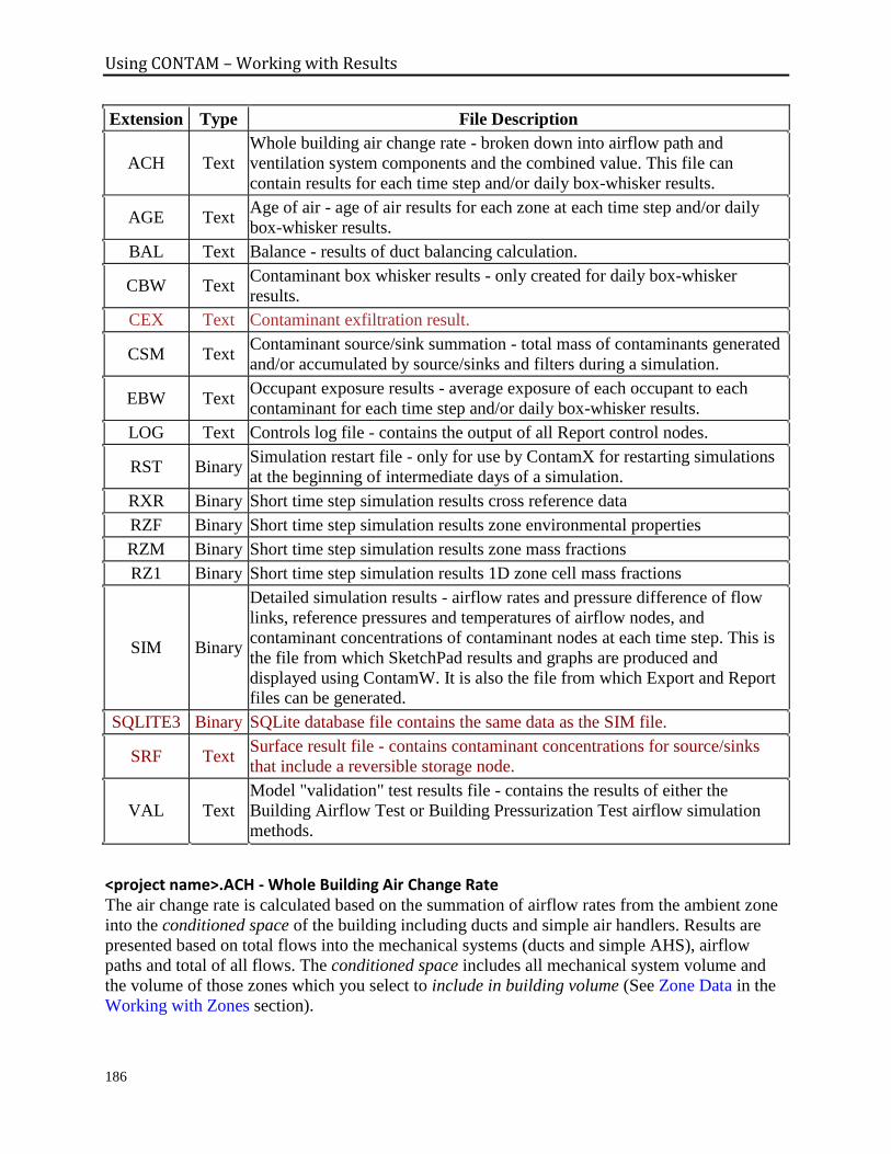
Using CONTAM – Working with Results
186
Extension Type File Description
ACH Text
Whole building air change rate - broken down into airflow path and
ventilation system components and the combined value. This file can
contain results for each time step and/or daily box-whisker results.
AGE Text Age of air - age of air results for each zone at each time step and/or daily
box-whisker results.
BAL Text Balance - results of duct balancing calculation.
CBW Text Contaminant box whisker results - only created for daily box-whisker
results.
CEX Text Contaminant exfiltration result.
CSM Text Contaminant source/sink summation - total mass of contaminants generated
and/or accumulated by source/sinks and filters during a simulation.
EBW Text Occupant exposure results - average exposure of each occupant to each
contaminant for each time step and/or daily box-whisker results.
LOG Text Controls log file - contains the output of all Report control nodes.
RST Binary Simulation restart file - only for use by ContamX for restarting simulations
at the beginning of intermediate days of a simulation.
RXR Binary Short time step simulation results cross reference data
RZF Binary Short time step simulation results zone environmental properties
RZM Binary Short time step simulation results zone mass fractions
RZ1 Binary Short time step simulation results 1D zone cell mass fractions
SIM Binary
Detailed simulation results - airflow rates and pressure difference of flow
links, reference pressures and temperatures of airflow nodes, and
contaminant concentrations of contaminant nodes at each time step. This is
the file from which SketchPad results and graphs are produced and
displayed using ContamW. It is also the file from which Export and Report
files can be generated.
SQLITE3 Binary SQLite database file contains the same data as the SIM file.
SRF Text Surface result file - contains contaminant concentrations for source/sinks
that include a reversible storage node.
VAL Text
Model "validation" test results file - contains the results of either the
Building Airflow Test or Building Pressurization Test airflow simulation
methods.
<project name>.ACH - Whole Building Air Change Rate The air change rate is calculated based on the summation of airflow rates from the ambient zone
into the conditioned space of the building including ducts and simple air handlers. Results are
presented based on total flows into the mechanical systems (ducts and simple AHS), airflow
paths and total of all flows. The conditioned space includes all mechanical system volume and
the volume of those zones which you select to include in building volume (See Zone Data in the
Working with Zones section).
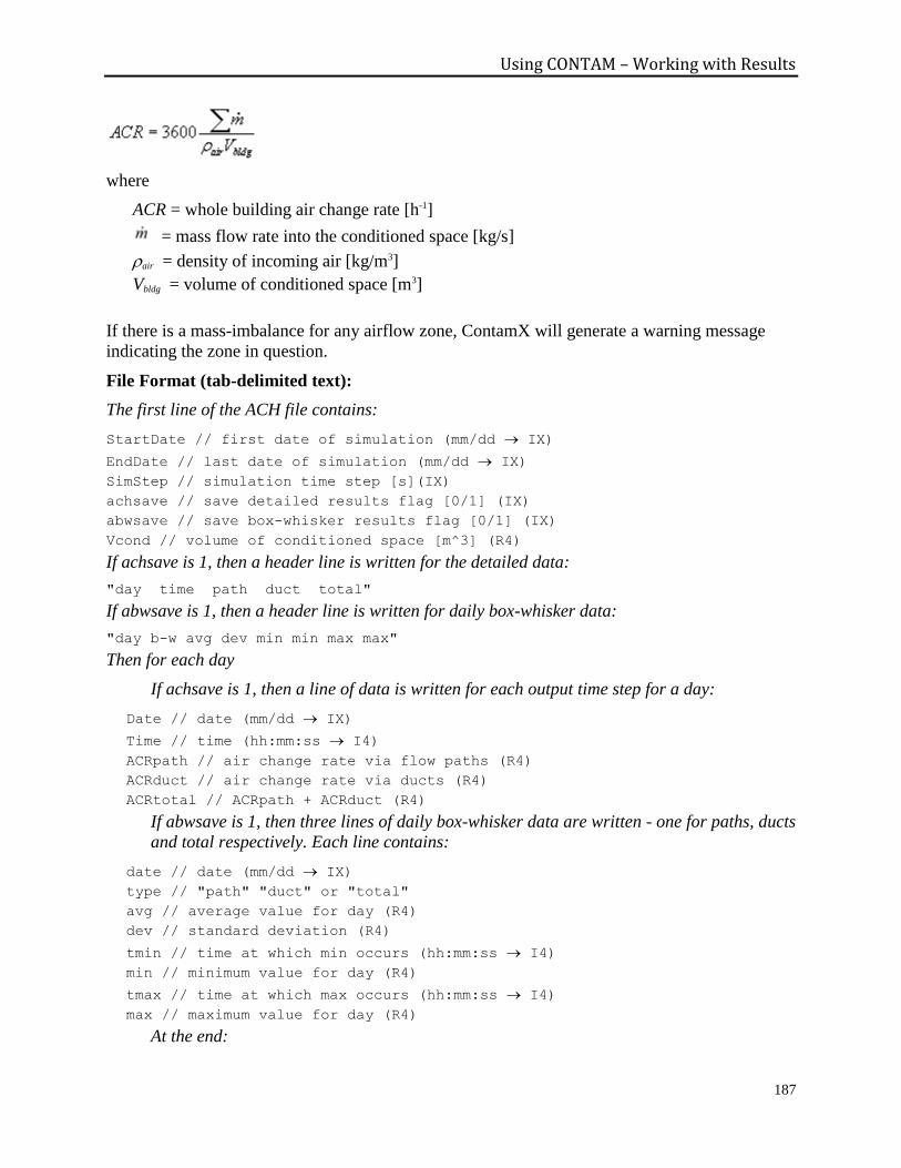
Using CONTAM – Working with Results
187
where
ACR = whole building air change rate [h-1]
= mass flow rate into the conditioned space [kg/s]
air = density of incoming air [kg/m3]
Vbldg = volume of conditioned space [m3]
If there is a mass-imbalance for any airflow zone, ContamX will generate a warning message
indicating the zone in question.
File Format (tab-delimited text):
The first line of the ACH file contains:
StartDate // first date of simulation (mm/dd IX)
EndDate // last date of simulation (mm/dd IX)
SimStep // simulation time step [s](IX)
achsave // save detailed results flag [0/1] (IX)
abwsave // save box-whisker results flag [0/1] (IX)
Vcond // volume of conditioned space [m^3] (R4)
If achsave is 1, then a header line is written for the detailed data:
"day time path duct total"
If abwsave is 1, then a header line is written for daily box-whisker data:
"day b-w avg dev min min max max"
Then for each day
If achsave is 1, then a line of data is written for each output time step for a day:
Date // date (mm/dd IX)
Time // time (hh:mm:ss I4)
ACRpath // air change rate via flow paths (R4)
ACRduct // air change rate via ducts (R4)
ACRtotal // ACRpath + ACRduct (R4)
If abwsave is 1, then three lines of daily box-whisker data are written - one for paths, ducts
and total respectively. Each line contains:
date // date (mm/dd IX)
type // "path" "duct" or "total"
avg // average value for day (R4)
dev // standard deviation (R4)
tmin // time at which min occurs (hh:mm:ss I4)
min // minimum value for day (R4)
tmax // time at which max occurs (hh:mm:ss I4)
max // maximum value for day (R4)
At the end:
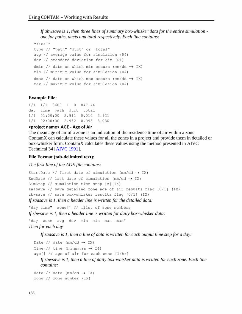
Using CONTAM – Working with Results
188
If abwsave is 1, then three lines of summary box-whisker data for the entire simulation -
one for paths, ducts and total respectively. Each line contains:
"final"
type // "path" "duct" or "total"
avg // average value for simulation (R4)
dev // standard deviation for sim (R4)
dmin // date on which min occurs (mm/dd IX)
min // minimum value for simulation (R4)
dmax // date on which max occurs (mm/dd IX)
max // maximum value for simulation (R4)
Example File:
1/1 1/1 3600 1 0 847.44
day time path duct total
1/1 01:00:00 2.911 0.010 2.921
1/1 02:00:00 2.932 0.098 3.030
<project name>.AGE - Age of Air The mean age of air of a zone is an indication of the residence time of air within a zone.
ContamX can calculate these values for all the zones in a project and provide them in detailed or
box-whisker form. ContamX calculates these values using the method presented in AIVC
Technical 34 [AIVC 1991].
File Format (tab-delimited text):
The first line of the AGE file contains:
StartDate // first date of simulation (mm/dd IX)
EndDate // last date of simulation (mm/dd IX)
SimStep // simulation time step [s](IX)
zaasave // save detailed zone age of air results flag [0/1] (IX)
zbwsave // save box-whisker results flag [0/1] (IX)
If zaasave is 1, then a header line is written for the detailed data:
"day time" zone[] // …list of zone numbers
If zbwsave is 1, then a header line is written for daily box-whisker data:
"day zone avg dev min min max max"
Then for each day
If zaasave is 1, then a line of data is written for each output time step for a day:
Date // date (mm/dd IX)
Time // time (hh:mm:ss I4)
age[] // age of air for each zone [1/hr]
If zbwsave is 1, then a line of daily box-whisker data is written for each zone. Each line
contains:
date // date (mm/dd IX)
zone // zone number (IX)
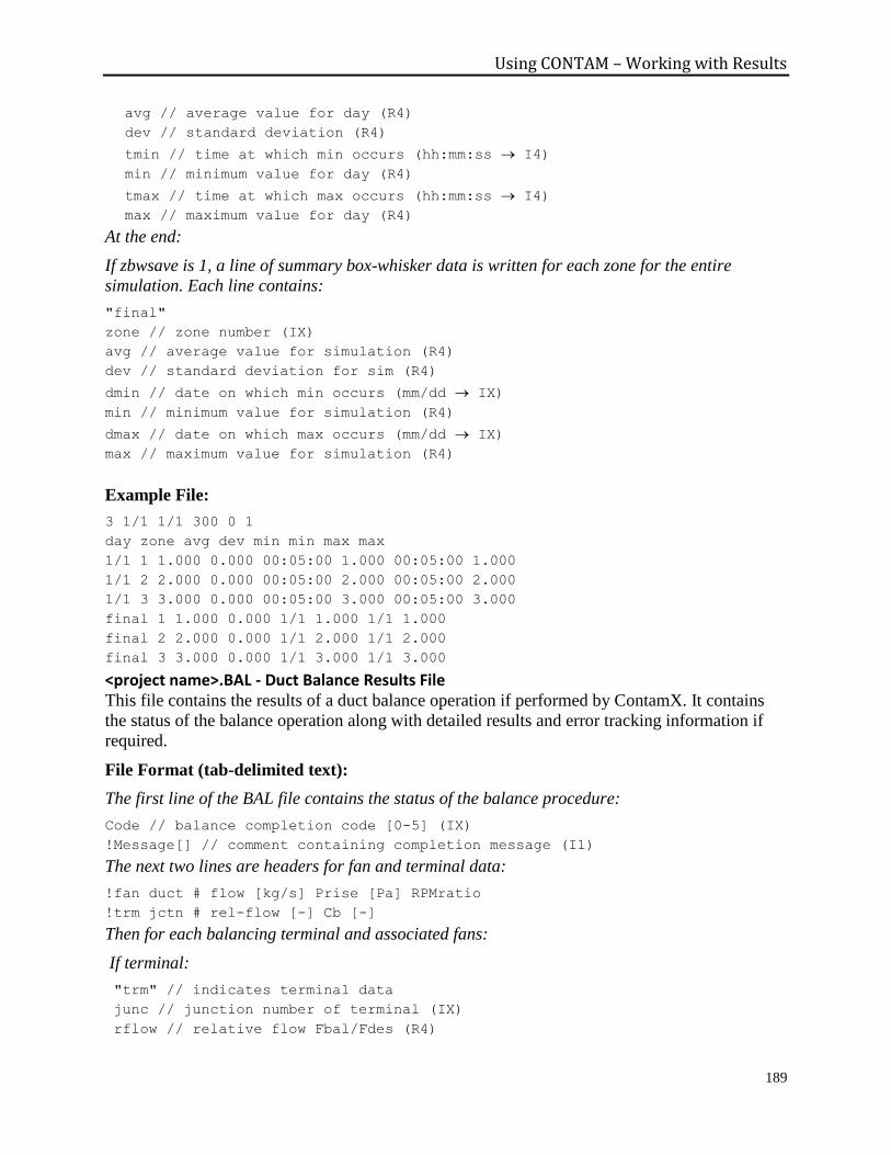
Using CONTAM – Working with Results
189
avg // average value for day (R4)
dev // standard deviation (R4)
tmin // time at which min occurs (hh:mm:ss I4)
min // minimum value for day (R4)
tmax // time at which max occurs (hh:mm:ss I4)
max // maximum value for day (R4)
At the end:
If zbwsave is 1, a line of summary box-whisker data is written for each zone for the entire
simulation. Each line contains:
"final"
zone // zone number (IX)
avg // average value for simulation (R4)
dev // standard deviation for sim (R4)
dmin // date on which min occurs (mm/dd IX)
min // minimum value for simulation (R4)
dmax // date on which max occurs (mm/dd IX)
max // maximum value for simulation (R4)
Example File:
3 1/1 1/1 300 0 1
day zone avg dev min min max max
1/1 1 1.000 0.000 00:05:00 1.000 00:05:00 1.000
1/1 2 2.000 0.000 00:05:00 2.000 00:05:00 2.000
1/1 3 3.000 0.000 00:05:00 3.000 00:05:00 3.000
final 1 1.000 0.000 1/1 1.000 1/1 1.000
final 2 2.000 0.000 1/1 2.000 1/1 2.000
final 3 3.000 0.000 1/1 3.000 1/1 3.000
<project name>.BAL - Duct Balance Results File This file contains the results of a duct balance operation if performed by ContamX. It contains
the status of the balance operation along with detailed results and error tracking information if
required.
File Format (tab-delimited text):
The first line of the BAL file contains the status of the balance procedure:
Code // balance completion code [0-5] (IX)
!Message[] // comment containing completion message (I1)
The next two lines are headers for fan and terminal data:
!fan duct # flow [kg/s] Prise [Pa] RPMratio
!trm jctn # rel-flow [-] Cb [-]
Then for each balancing terminal and associated fans:
If terminal:
"trm" // indicates terminal data
junc // junction number of terminal (IX)
rflow // relative flow Fbal/Fdes (R4)
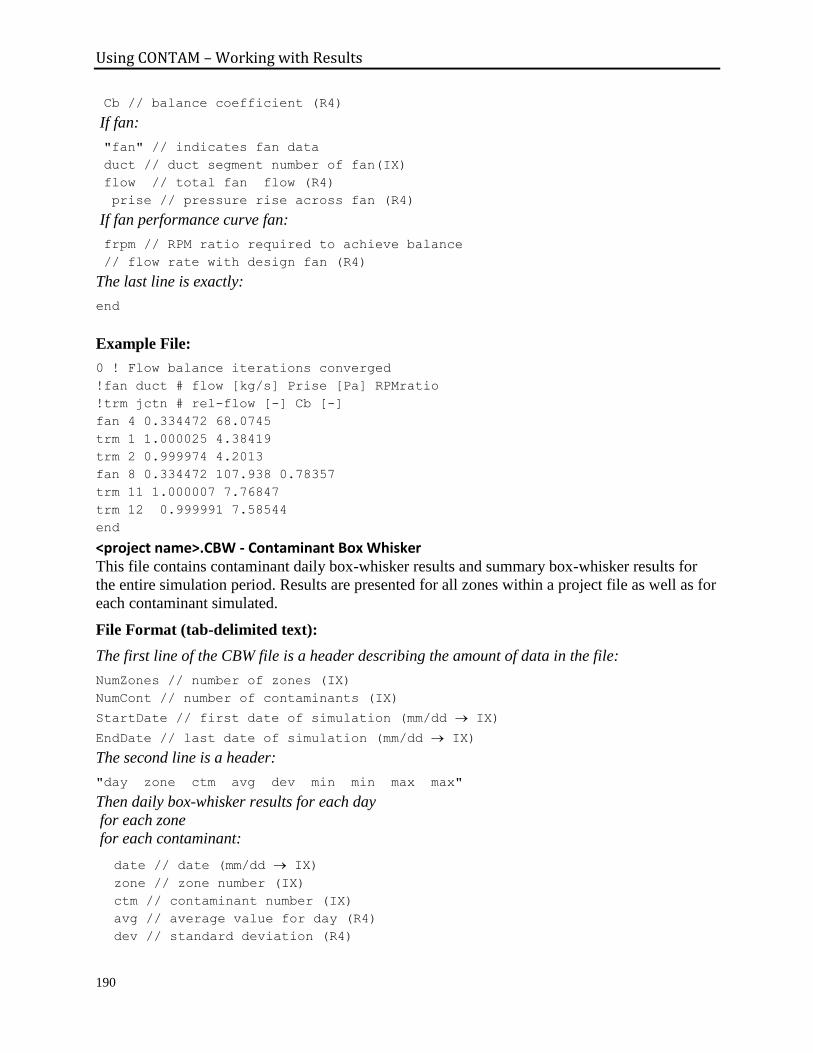
Using CONTAM – Working with Results
190
Cb // balance coefficient (R4)
If fan:
"fan" // indicates fan data
duct // duct segment number of fan(IX)
flow // total fan flow (R4)
prise // pressure rise across fan (R4)
If fan performance curve fan:
frpm // RPM ratio required to achieve balance
// flow rate with design fan (R4)
The last line is exactly:
end
Example File:
0 ! Flow balance iterations converged
!fan duct # flow [kg/s] Prise [Pa] RPMratio
!trm jctn # rel-flow [-] Cb [-]
fan 4 0.334472 68.0745
trm 1 1.000025 4.38419
trm 2 0.999974 4.2013
fan 8 0.334472 107.938 0.78357
trm 11 1.000007 7.76847
trm 12 0.999991 7.58544
end
<project name>.CBW - Contaminant Box Whisker This file contains contaminant daily box-whisker results and summary box-whisker results for
the entire simulation period. Results are presented for all zones within a project file as well as for
each contaminant simulated.
File Format (tab-delimited text):
The first line of the CBW file is a header describing the amount of data in the file:
NumZones // number of zones (IX)
NumCont // number of contaminants (IX)
StartDate // first date of simulation (mm/dd IX)
EndDate // last date of simulation (mm/dd IX)
The second line is a header:
"day zone ctm avg dev min min max max"
Then daily box-whisker results for each day
for each zone
for each contaminant:
date // date (mm/dd IX)
zone // zone number (IX)
ctm // contaminant number (IX)
avg // average value for day (R4)
dev // standard deviation (R4)
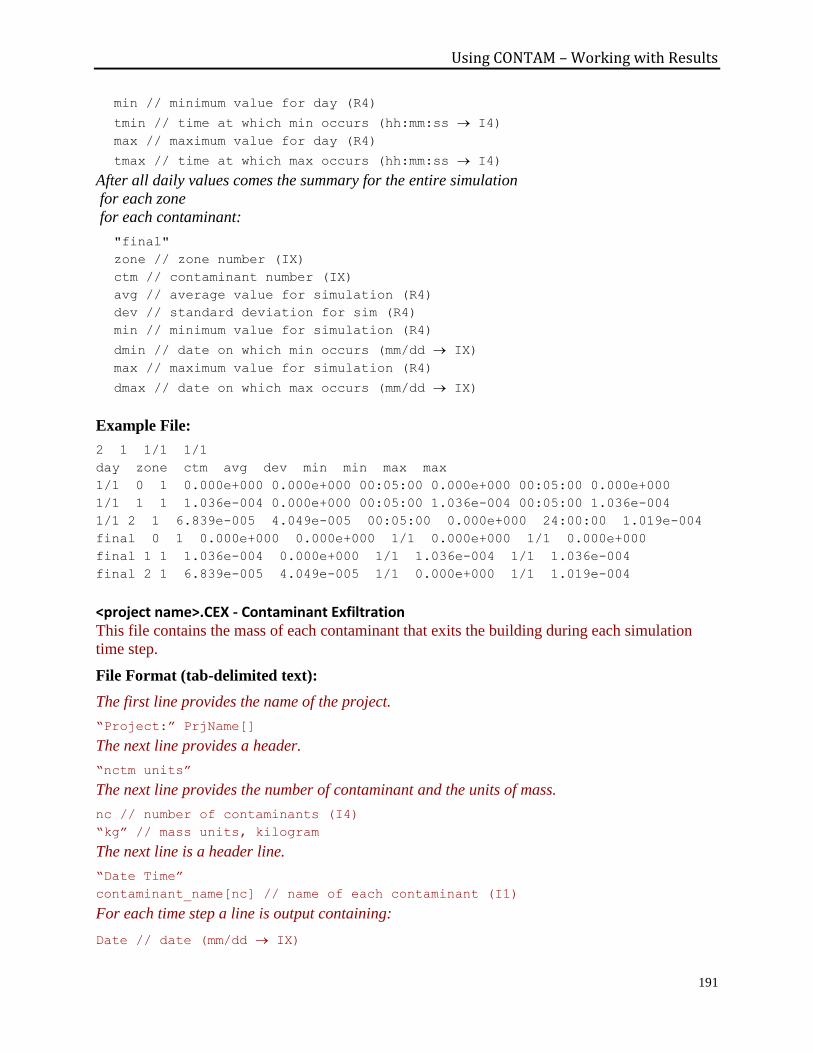
Using CONTAM – Working with Results
191
min // minimum value for day (R4)
tmin // time at which min occurs (hh:mm:ss I4)
max // maximum value for day (R4)
tmax // time at which max occurs (hh:mm:ss I4)
After all daily values comes the summary for the entire simulation
for each zone
for each contaminant:
"final"
zone // zone number (IX)
ctm // contaminant number (IX)
avg // average value for simulation (R4)
dev // standard deviation for sim (R4)
min // minimum value for simulation (R4)
dmin // date on which min occurs (mm/dd IX)
max // maximum value for simulation (R4)
dmax // date on which max occurs (mm/dd IX)
Example File:
2 1 1/1 1/1
day zone ctm avg dev min min max max
1/1 0 1 0.000e+000 0.000e+000 00:05:00 0.000e+000 00:05:00 0.000e+000
1/1 1 1 1.036e-004 0.000e+000 00:05:00 1.036e-004 00:05:00 1.036e-004
1/1 2 1 6.839e-005 4.049e-005 00:05:00 0.000e+000 24:00:00 1.019e-004
final 0 1 0.000e+000 0.000e+000 1/1 0.000e+000 1/1 0.000e+000
final 1 1 1.036e-004 0.000e+000 1/1 1.036e-004 1/1 1.036e-004
final 2 1 6.839e-005 4.049e-005 1/1 0.000e+000 1/1 1.019e-004
<project name>.CEX - Contaminant Exfiltration This file contains the mass of each contaminant that exits the building during each simulation
time step.
File Format (tab-delimited text):
The first line provides the name of the project.
“Project:” PrjName[]
The next line provides a header.
“nctm units”
The next line provides the number of contaminant and the units of mass.
nc // number of contaminants (I4)
“kg” // mass units, kilogram
The next line is a header line.
“Date Time”
contaminant_name[nc] // name of each contaminant (I1)
For each time step a line is output containing:
Date // date (mm/dd IX)
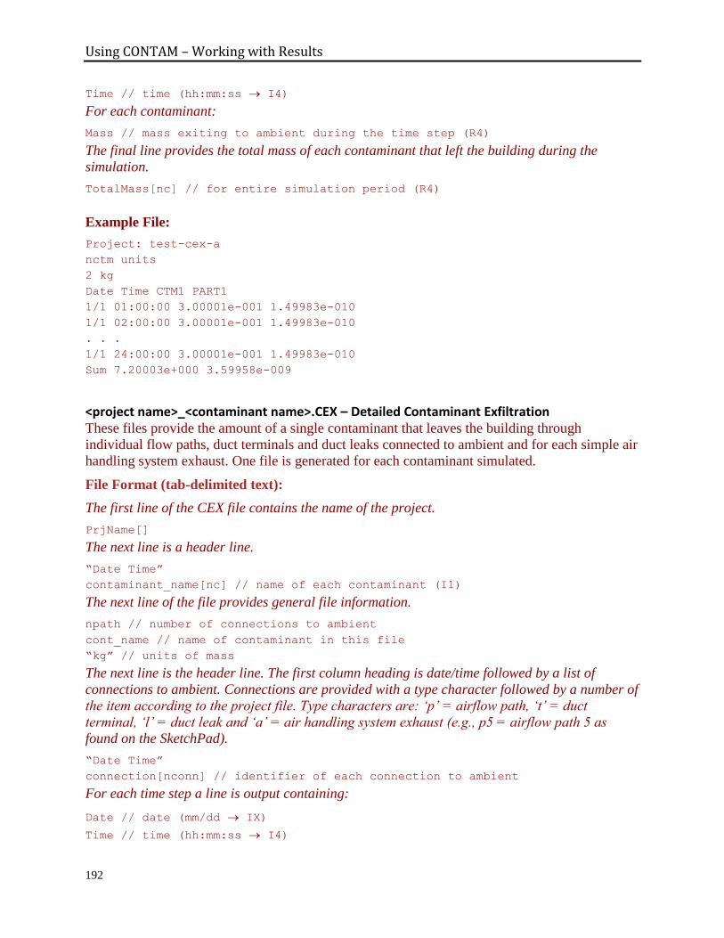
Using CONTAM – Working with Results
192
Time // time (hh:mm:ss I4)
For each contaminant:
Mass // mass exiting to ambient during the time step (R4)
The final line provides the total mass of each contaminant that left the building during the
simulation.
TotalMass[nc] // for entire simulation period (R4)
Example File:
Project: test-cex-a
nctm units
2 kg
Date Time CTM1 PART1
1/1 01:00:00 3.00001e-001 1.49983e-010
1/1 02:00:00 3.00001e-001 1.49983e-010
. . .
1/1 24:00:00 3.00001e-001 1.49983e-010
Sum 7.20003e+000 3.59958e-009
<project name>_<contaminant name>.CEX – Detailed Contaminant Exfiltration These files provide the amount of a single contaminant that leaves the building through
individual flow paths, duct terminals and duct leaks connected to ambient and for each simple air
handling system exhaust. One file is generated for each contaminant simulated.
File Format (tab-delimited text):
The first line of the CEX file contains the name of the project.
PrjName[]
The next line is a header line.
“Date Time”
contaminant_name[nc] // name of each contaminant (I1)
The next line of the file provides general file information.
npath // number of connections to ambient
cont_name // name of contaminant in this file
“kg” // units of mass
The next line is the header line. The first column heading is date/time followed by a list of
connections to ambient. Connections are provided with a type character followed by a number of
the item according to the project file. Type characters are: ‘p’ = airflow path, ‘t’ = duct
terminal, ‘l’ = duct leak and ‘a’ = air handling system exhaust (e.g., p5 = airflow path 5 as
found on the SketchPad).
“Date Time”
connection[nconn] // identifier of each connection to ambient
For each time step a line is output containing:
Date // date (mm/dd IX)
Time // time (hh:mm:ss I4)
Using CONTAM – Working with Results
193
For each connection:
Mass // mass exiting through given connection during time step (R4)
Example File:
Project: test-cex-a
npath ctm_name units
4 CTM1 kg
Date Time p1 p2 a1 t2
1/1 01:00:00 0.00000e+000 1.00000e-001 1.00000e-001 1.00000e-001
1/1 02:00:00 0.00000e+000 1.00000e-001 1.00000e-001 1.00000e-001
. . .
1/1 24:00:00 0.00000e+000 1.00000e-001 1.00000e-001 1.00000e-001
<project name>.CSM - Contaminant Source/Sink Summation This file contains summary data related to contaminant simulation. This file is created
automatically by ContamX whenever transient contaminant simulations are performed.
Source/sink, filter and zone numbers are provided for referencing back to ContamW. The file
consists of six sections:
Contaminant source/sink summary - This section provides the mass of contaminant generated,
removed and stored for each source/sink during a simulation.
Filter challenge summary - This section provides the mass of contaminant to which each filter is
exposed during a simulation (upstream challenge).
Filter loading summary - This section provides the mass of contaminant "loaded" onto each filter
during a simulation (not including initial loading).
Filter breakthrough summary - This section provides indication of whether or not filter
breakthrough applies. If breakthrough applies and occurs then the date and time when it occurs
and the breakthrough efficiency are provided, otherwise the efficiency at the end of the
simulation is provided. Breakthrough only applies to Simple Gaseous Filters for which a non-
zero breakthrough efficiency is provided.
Interactions with ambient - This section provides the mass of each contaminant that enters and
exits the building volume, i.e., those that are set to be included in the building volume.
Simulation time - This section provides information on the duration of the simulation.
File Format (tab-delimited text):
The first two lines of the CSM file display the PRJ file name and the date and time the simulation
was run:
"Project:" FilePath[] // the full path of the PRJ file (I1)
"Time:" SimTime[] // PC time the simulation was started (I1)
-- Blank line --
This is followed by the number of contaminants simulated.
NumCont "contaminants" // number of contaminants (I4)
-- Blank line --
This is followed by the Contaminant source/sink summary section.
NOTE: the following section is only presented if source/sinks exist within the PRJ file.
Using CONTAM – Working with Results
194
The first line of the source/sink section is a header:
"Contaminant source/sink summary."
The next line contains the number of source/sinks:
NumSS "source/sinks" // number of source/sinks(IX)
The next line is a header:
s/s# zn# species released removed stored [kg]
Then a line of data for each source/sink:
SSNum // source/sink number (IX)
Type[] // source/sink type (I1)
Name[] // contaminant name (I1)
ZoneNum // zone number (IX)
As // surface area of deposition elements [m^2] (R4)
mult // multiplier (R4)
Xmin // location coordinates [m] (R4)
Xmax
Ymin
Ymax
Zmin
Zmax
MassRel // mass released(R4)
MassRem // mass removed [kg] (R4)
MassAcc // mass accumulated including previous storage (R4)
-- Blank line ---
This is followed by the Filter challenge section.
NOTE: this section is only presented if filters exist within the PRJ file.
The first line of the section is a header:
"Filter challenge summary."
The next line contains the number of filters:
NumFilt "filters" // number of filters (IX)
The next line is a header:
"path" Ctm[nc] "element" // Ctm[nc] is a list of contaminants
// where nc is the number of contaminants.
Then two lines of data for each filter:
The first line is:
FltNum // number of flow component that contains the filter
// and letter indicating type (p:path, d:duct, t:term)
MassUp[nc] // challenge mass of each contaminant [kg] (R4)
Name[] // filter element name (I1)
The second line is: "--" // indicates same filter as previous
MassDown[nc] // unfiltered mass of each contaminant [kg] (R4)
"downstream" // indicates downstream mass
-- Blank line --
Using CONTAM – Working with Results
195
This is followed by the Filter loading section.
NOTE: this section is only presented if filters exist within the PRJ file.
The first line of the section is a header:
"Filter loading summary."
The next line contains the number of filters:
NumFilt // number of filters (IX)
The next line is a header:
"path" Ctm[nc] "element ns" // Ctm[nc] is a list of contaminants
// nc is the number of contaminants.
Then a line of data for each filter: FltNum // number of flow component that contains the filter
// and letter indicating type (p:path, d:duct, t:terminal)
MassLoad[nc] // mass filtered during simulation [kg] (R4)
Name[] // filter element name (I1)
ns // number of sub-elements, ns>0 for super-filter (I4)
If ns>0, then a line of data for each sub-filter of the super-filter:
"--" // indicates sub-filter
MassLoad[nc] // mass filtered during simulation [kg] (R4)
Name[] // filter element name (I1)
"0" // zero sub-elements (I4)
-- Blank line --
This is followed by the Filter breakthrough section.
NOTE: this section is only presented if filters exist within the PRJ file.
The first line of the section is a header:
"Filter breakthrough summary."
The next line contains the number of filters:
NumFilt "filters" // number of filters for which for which
// breakthrough is possible, currently on Simple
// Gaseous types (IX)
The next two lines are headers:
"path element"
" contaminant date time efficiency"
Then a line of data for each filter:
FltNum // number of flow component that contains the filter
// and letter indicating type (p:path, d:duct, t:terminal)
Name[] // filter element name (I1)
nc // number of contaminants (I4)
Then a line of data for each contaminant for which breakthrough is specified.
Each line contains:
"--" // indicates continuation of filter
Ctm[] // contaminant name (I1)
If breakthrough occurred:
Date[] // date on which breakthrough occurs (MMMDD I4)
Using CONTAM – Working with Results
196
Time // time at which breakthrough occurs (hh:mm:ss I4)
bkeff // breakthrough efficiency
If breakthrough does not occur: "--" // indicates no breakthrough date
"--" // indicates no breakthrough time
eff // efficiency at end of simulation
-- Blank line --
This is followed by the Interactions with ambient section.
The next two lines of the section are headers. They are exactly:
"Interactions with ambient."
"contaminant flow from flow to [kg]"
Then a line of data for each contaminant:
Ctm[] // contaminant name (I1)
MassFrom // total mass entering from ambient zone [kg] (R4)
MassTo // total mass exiting to ambient zone [kg] (R4)
-- Blank line --
The final section is the Simulation time section:
It contains a header and three lines of data:
"Simulation time:"
tsec "seconds" // simulation time in seconds [s] (IX)
thr "hours," // simulation time in hours [h] (R4)
tday "days" // simulation time in days [days] (R4)
Example File:
Project: C:\CONTAM96\samples\.4\Filters\TestBK3.prj
Time: Mon Jul 18 10:17:22 2005
5 contaminants
Contaminant source/sink summary.
4 source/sinks
s/s# type species zn# As mult Xmin Xmax Ymin Ymax Zmin Zmax released removed
stored [kg]
1 ccf CO 3 0 1 0 0 0 0 0 0 7.20E-01 0.00E+00 0
2 brs Cl2 3 0 1 0 0 0 0 0 0 1.00E-04 0.00E+00 0
4 drs Cl2 4 0 1 0 0 0 0 0 0 0.00E+00 1.04E-01 0
3 bls Cl2 4 1 1 0 0 0 0 0 0 8.66E-03 8.67E-03 1.23E-05
Filter challenge summary.
3 filters
path CO CO2 Cl2 part0.10 part1.00 element
6p 1.164e-001 1.829e+000 2.361e-001 1.204e-001 1.204e-001 Both
-- 6.215e-002 1.829e+000 1.079e-001 1.039e-001 7.389e-002 downstream
1d 1.164e-001 1.829e+000 2.361e-001 1.204e-001 1.204e-001 MERV10
-- 1.164e-001 1.829e+000 2.361e-001 1.039e-001 7.389e-002 downstream
2t 1.164e-001 1.829e+000 2.361e-001 1.039e-001 7.388e-002 GF0
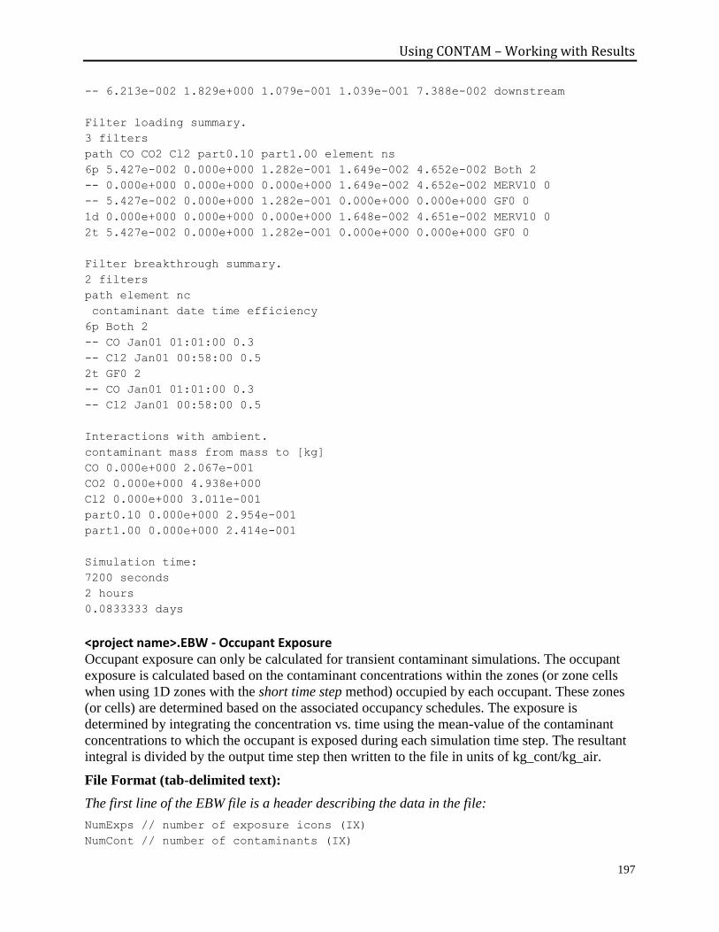
Using CONTAM – Working with Results
197
-- 6.213e-002 1.829e+000 1.079e-001 1.039e-001 7.388e-002 downstream
Filter loading summary.
3 filters
path CO CO2 Cl2 part0.10 part1.00 element ns
6p 5.427e-002 0.000e+000 1.282e-001 1.649e-002 4.652e-002 Both 2
-- 0.000e+000 0.000e+000 0.000e+000 1.649e-002 4.652e-002 MERV10 0
-- 5.427e-002 0.000e+000 1.282e-001 0.000e+000 0.000e+000 GF0 0
1d 0.000e+000 0.000e+000 0.000e+000 1.648e-002 4.651e-002 MERV10 0
2t 5.427e-002 0.000e+000 1.282e-001 0.000e+000 0.000e+000 GF0 0
Filter breakthrough summary.
2 filters
path element nc
contaminant date time efficiency
6p Both 2
-- CO Jan01 01:01:00 0.3
-- Cl2 Jan01 00:58:00 0.5
2t GF0 2
-- CO Jan01 01:01:00 0.3
-- Cl2 Jan01 00:58:00 0.5
Interactions with ambient.
contaminant mass from mass to [kg]
CO 0.000e+000 2.067e-001
CO2 0.000e+000 4.938e+000
Cl2 0.000e+000 3.011e-001
part0.10 0.000e+000 2.954e-001
part1.00 0.000e+000 2.414e-001
Simulation time:
7200 seconds
2 hours
0.0833333 days
<project name>.EBW - Occupant Exposure Occupant exposure can only be calculated for transient contaminant simulations. The occupant
exposure is calculated based on the contaminant concentrations within the zones (or zone cells
when using 1D zones with the short time step method) occupied by each occupant. These zones
(or cells) are determined based on the associated occupancy schedules. The exposure is
determined by integrating the concentration vs. time using the mean-value of the contaminant
concentrations to which the occupant is exposed during each simulation time step. The resultant
integral is divided by the output time step then written to the file in units of kg_cont/kg_air.
File Format (tab-delimited text):
The first line of the EBW file is a header describing the data in the file:
NumExps // number of exposure icons (IX)
NumCont // number of contaminants (IX)
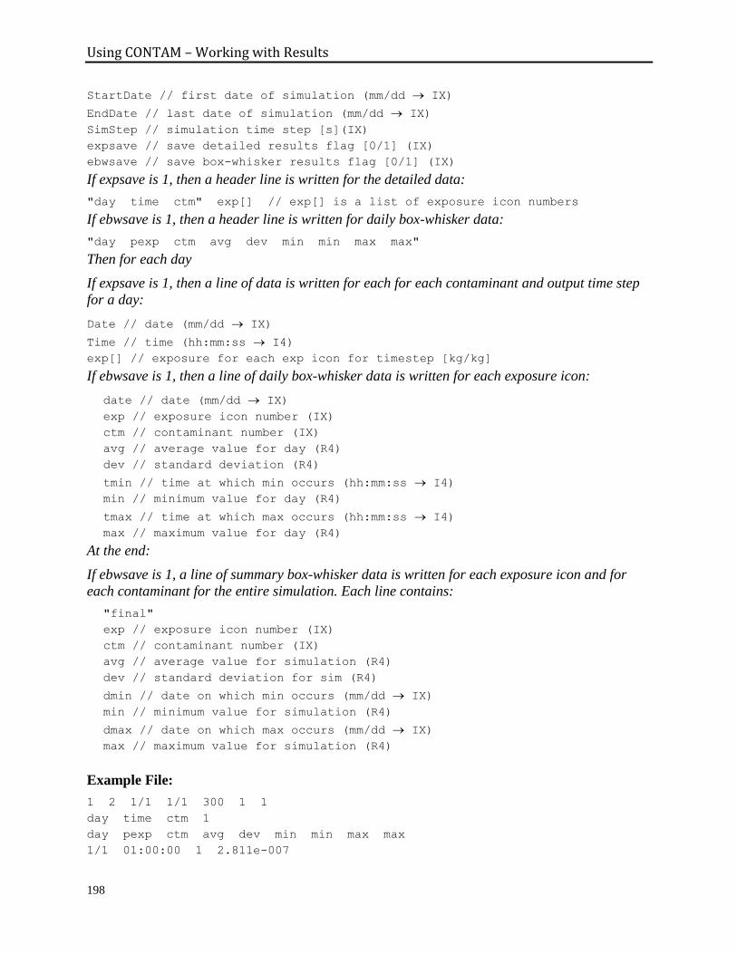
Using CONTAM – Working with Results
198
StartDate // first date of simulation (mm/dd IX)
EndDate // last date of simulation (mm/dd IX)
SimStep // simulation time step [s](IX)
expsave // save detailed results flag [0/1] (IX)
ebwsave // save box-whisker results flag [0/1] (IX)
If expsave is 1, then a header line is written for the detailed data:
"day time ctm" exp[] // exp[] is a list of exposure icon numbers
If ebwsave is 1, then a header line is written for daily box-whisker data:
"day pexp ctm avg dev min min max max"
Then for each day
If expsave is 1, then a line of data is written for each for each contaminant and output time step
for a day:
Date // date (mm/dd IX)
Time // time (hh:mm:ss I4)
exp[] // exposure for each exp icon for timestep [kg/kg]
If ebwsave is 1, then a line of daily box-whisker data is written for each exposure icon:
date // date (mm/dd IX)
exp // exposure icon number (IX)
ctm // contaminant number (IX)
avg // average value for day (R4)
dev // standard deviation (R4)
tmin // time at which min occurs (hh:mm:ss I4)
min // minimum value for day (R4)
tmax // time at which max occurs (hh:mm:ss I4)
max // maximum value for day (R4)
At the end:
If ebwsave is 1, a line of summary box-whisker data is written for each exposure icon and for
each contaminant for the entire simulation. Each line contains:
"final"
exp // exposure icon number (IX)
ctm // contaminant number (IX)
avg // average value for simulation (R4)
dev // standard deviation for sim (R4)
dmin // date on which min occurs (mm/dd IX)
min // minimum value for simulation (R4)
dmax // date on which max occurs (mm/dd IX)
max // maximum value for simulation (R4)
Example File:
1 2 1/1 1/1 300 1 1
day time ctm 1
day pexp ctm avg dev min min max max
1/1 01:00:00 1 2.811e-007
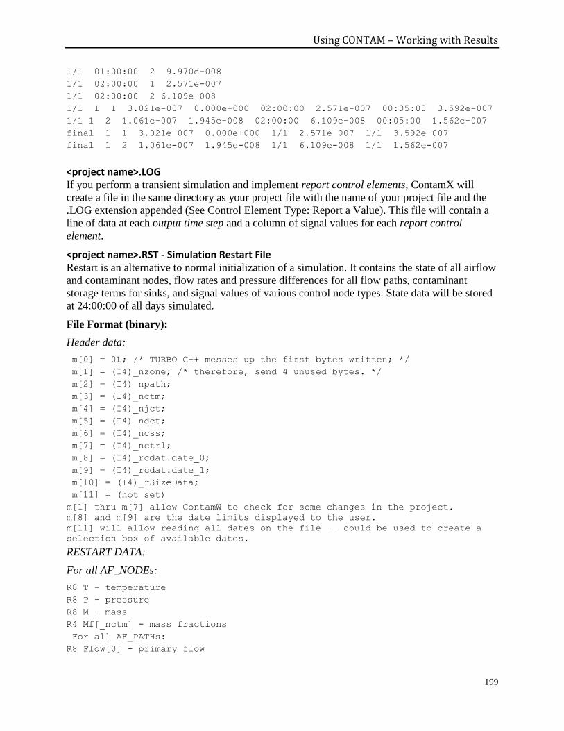
Using CONTAM – Working with Results
199
1/1 01:00:00 2 9.970e-008
1/1 02:00:00 1 2.571e-007
1/1 02:00:00 2 6.109e-008
1/1 1 1 3.021e-007 0.000e+000 02:00:00 2.571e-007 00:05:00 3.592e-007
1/1 1 2 1.061e-007 1.945e-008 02:00:00 6.109e-008 00:05:00 1.562e-007
final 1 1 3.021e-007 0.000e+000 1/1 2.571e-007 1/1 3.592e-007
final 1 2 1.061e-007 1.945e-008 1/1 6.109e-008 1/1 1.562e-007
<project name>.LOG If you perform a transient simulation and implement report control elements, ContamX will
create a file in the same directory as your project file with the name of your project file and the
.LOG extension appended (See Control Element Type: Report a Value). This file will contain a
line of data at each output time step and a column of signal values for each report control
element.
<project name>.RST - Simulation Restart File Restart is an alternative to normal initialization of a simulation. It contains the state of all airflow
and contaminant nodes, flow rates and pressure differences for all flow paths, contaminant
storage terms for sinks, and signal values of various control node types. State data will be stored
at 24:00:00 of all days simulated.
File Format (binary):
Header data:
m[0] = 0L; /* TURBO C++ messes up the first bytes written; */
m[1] = (I4)_nzone; /* therefore, send 4 unused bytes. */
m[2] = (I4)_npath;
m[3] = (I4)_nctm;
m[4] = (I4)_njct;
m[5] = (I4)_ndct;
m[6] = (I4)_ncss;
m[7] = (I4)_nctrl;
m[8] = (I4)_rcdat.date_0;
m[9] = (I4)_rcdat.date_1;
m[10] = (I4)_rSizeData;
m[11] = (not set)
m[1] thru m[7] allow ContamW to check for some changes in the project.
m[8] and m[9] are the date limits displayed to the user.
m[11] will allow reading all dates on the file -- could be used to create a
selection box of available dates.
RESTART DATA:
For all AF_NODEs:
R8 T - temperature
R8 P - pressure
R8 M - mass
R4 Mf[_nctm] - mass fractions
For all AF_PATHs:
R8 Flow[0] - primary flow
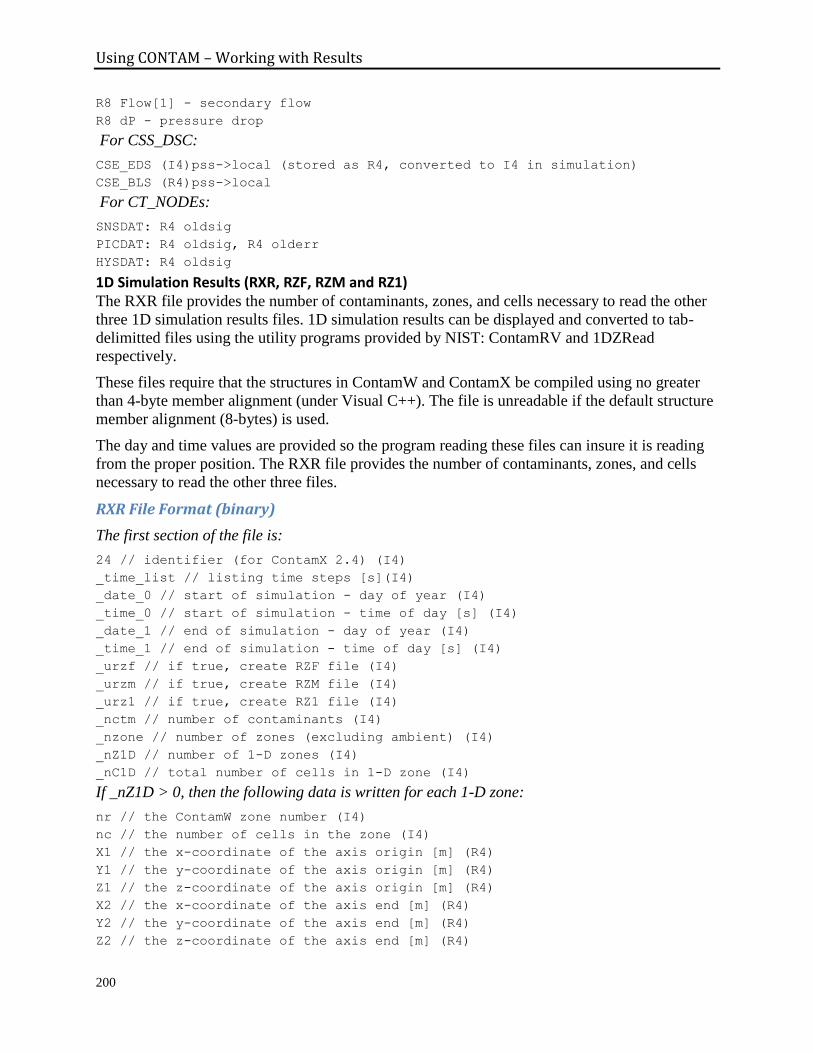
Using CONTAM – Working with Results
200
R8 Flow[1] - secondary flow
R8 dP - pressure drop
For CSS_DSC:
CSE_EDS (I4)pss->local (stored as R4, converted to I4 in simulation)
CSE_BLS (R4)pss->local
For CT_NODEs:
SNSDAT: R4 oldsig
PICDAT: R4 oldsig, R4 olderr
HYSDAT: R4 oldsig
1D Simulation Results (RXR, RZF, RZM and RZ1) The RXR file provides the number of contaminants, zones, and cells necessary to read the other
three 1D simulation results files. 1D simulation results can be displayed and converted to tab-
delimitted files using the utility programs provided by NIST: ContamRV and 1DZRead
respectively.
These files require that the structures in ContamW and ContamX be compiled using no greater
than 4-byte member alignment (under Visual C++). The file is unreadable if the default structure
member alignment (8-bytes) is used.
The day and time values are provided so the program reading these files can insure it is reading
from the proper position. The RXR file provides the number of contaminants, zones, and cells
necessary to read the other three files.
RXR File Format (binary)
The first section of the file is:
24 // identifier (for ContamX 2.4) (I4)
_time_list // listing time steps [s](I4)
_date_0 // start of simulation - day of year (I4)
_time_0 // start of simulation - time of day [s] (I4)
_date_1 // end of simulation - day of year (I4)
_time_1 // end of simulation - time of day [s] (I4)
_urzf // if true, create RZF file (I4)
_urzm // if true, create RZM file (I4)
_urz1 // if true, create RZ1 file (I4)
_nctm // number of contaminants (I4)
_nzone // number of zones (excluding ambient) (I4)
_nZ1D // number of 1-D zones (I4)
_nC1D // total number of cells in 1-D zone (I4)
If _nZ1D > 0, then the following data is written for each 1-D zone:
nr // the ContamW zone number (I4)
nc // the number of cells in the zone (I4)
X1 // the x-coordinate of the axis origin [m] (R4)
Y1 // the y-coordinate of the axis origin [m] (R4)
Z1 // the z-coordinate of the axis origin [m] (R4)
X2 // the x-coordinate of the axis end [m] (R4)
Y2 // the y-coordinate of the axis end [m] (R4)
Z2 // the z-coordinate of the axis end [m] (R4)
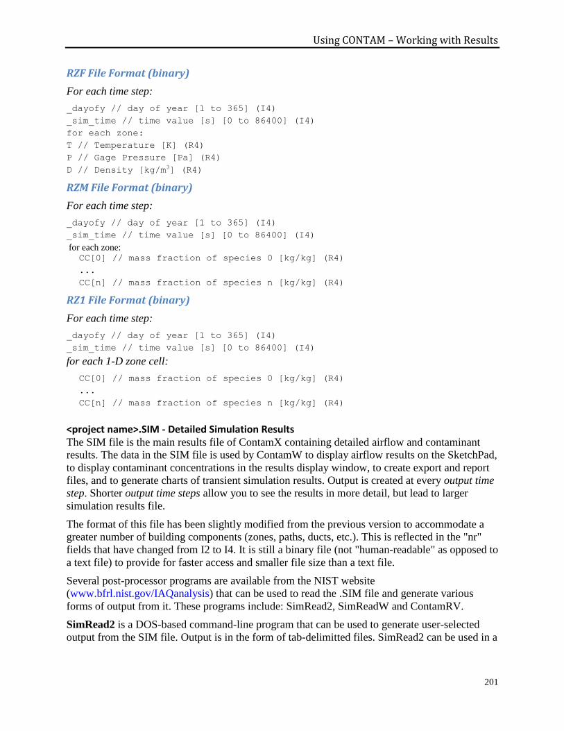
Using CONTAM – Working with Results
201
RZF File Format (binary)
For each time step:
_dayofy // day of year [1 to 365] (I4)
_sim_time // time value [s] [0 to 86400] (I4)
for each zone:
T // Temperature [K] (R4)
P // Gage Pressure [Pa] (R4)
D // Density [kg/m3] (R4)
RZM File Format (binary)
For each time step:
_dayofy // day of year [1 to 365] (I4)
_sim_time // time value [s] [0 to 86400] (I4)
for each zone: CC[0] // mass fraction of species 0 [kg/kg] (R4)
...
CC[n] // mass fraction of species n [kg/kg] (R4)
RZ1 File Format (binary)
For each time step:
_dayofy // day of year [1 to 365] (I4)
_sim_time // time value [s] [0 to 86400] (I4)
for each 1-D zone cell:
CC[0] // mass fraction of species 0 [kg/kg] (R4)
...
CC[n] // mass fraction of species n [kg/kg] (R4)
<project name>.SIM - Detailed Simulation Results The SIM file is the main results file of ContamX containing detailed airflow and contaminant
results. The data in the SIM file is used by ContamW to display airflow results on the SketchPad,
to display contaminant concentrations in the results display window, to create export and report
files, and to generate charts of transient simulation results. Output is created at every output time
step. Shorter output time steps allow you to see the results in more detail, but lead to larger
simulation results file.
The format of this file has been slightly modified from the previous version to accommodate a
greater number of building components (zones, paths, ducts, etc.). This is reflected in the "nr"
fields that have changed from I2 to I4. It is still a binary file (not "human-readable" as opposed to
a text file) to provide for faster access and smaller file size than a text file.
Several post-processor programs are available from the NIST website
(www.bfrl.nist.gov/IAQanalysis) that can be used to read the .SIM file and generate various
forms of output from it. These programs include: SimRead2, SimReadW and ContamRV.
SimRead2 is a DOS-based command-line program that can be used to generate user-selected
output from the SIM file. Output is in the form of tab-delimitted files. SimRead2 can be used in a
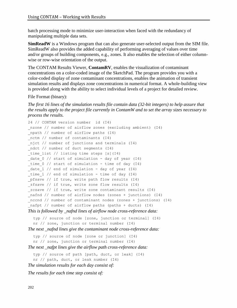
Using CONTAM – Working with Results
202
batch processing mode to minimize user-interaction when faced with the redundancy of
manipulating multiple data sets.
SimReadW is a Windows program that can also generate user-selected output from the SIM file.
SimReadW also provides the added capability of performing averaging of values over time
and/or groups of building components, e.g., zones. It also enables the selection of either column-
wise or row-wise orientation of the output.
The CONTAM Results Viewer, ContamRV, enables the visualization of contaminant
concentrations on a color-coded image of the SketchPad. The program provides you with a
color-coded display of zone contaminant concentrations, enables the animation of transient
simulation results and displays zone concentrations in numerical format. A whole-building view
is provided along with the ability to select individual levels of a project for detailed review.
File Format (binary):
The first 16 lines of the simulation results file contain data (32-bit integers) to help assure that
the results apply to the project file currently in ContamW and to set the array sizes necessary to
process the results.
24 // CONTAM version number id (I4)
_nzone // number of airflow zones (excluding ambient) (I4)
_npath // number of airflow paths (I4)
_nctm // number of contaminants (I4)
_njct // number of junctions and terminals (I4)
_ndct // number of duct segments (I4)
_time_list // listing time steps [s](I4)
_date_0 // start of simulation - day of year (I4)
_time_0 // start of simulation - time of day (I4)
_date_1 // end of simulation - day of year (I4)
_time_1 // end of simulation - time of day (I4)
_pfsave // if true, write path flow results (I4)
_zfsave // if true, write zone flow results (I4)
_zcsave // if true, write zone contaminant results (I4)
_nafnd // number of airflow nodes (zones + junctions) (I4)
_nccnd // number of contaminant nodes (zones + junctions) (I4)
_nafpt // number of airflow paths (paths + ducts) (I4)
This is followed by _nafnd lines of airflow node cross-reference data:
typ // source of node [zone, junction or terminal] (I4)
nr // zone, junction or terminal number (I4)
The next _nafnd lines give the contaminant node cross-reference data:
typ // source of node [zone or junction] (I4)
nr // zone, junction or terminal number (I4)
The next _nafpt lines give the airflow path cross-reference data:
typ // source of path [path, duct, or leak] (I4)
nr // path, duct, or leak number (I4)
The simulation results for each day consist of:
The results for each time step consist of:

Using CONTAM – Working with Results
203
A line of time and ambient data:
dayofy // day of year [1 to 365] (I2)
daytyp // type of day [1 to 12] (I2)
sim_time // time value [s] [0 to 86400] (I4)
Tambt // ambient temperature [k] (R4)
P // barometric pressure [Pa] (R4)
Ws // wind speed [m/s] (R4)
Wd // wind angle [deg] (R4)
CC[0] // ambient mass fraction of species 0 [kg/kg] (R4)
...
CC[n] // ambient mass fraction of species n [kg/kg] (R4)
A line of data for each airflow path:
nr // path number; use as check (I4)
dP // pressure drop across path [Pa] (R4)
Flow0 // primary flow value [kg/s] (R4)
Flow1 // alternate flow value [kg/s] (R4)
A line of data for each airflow node (excluding ambient):
nr // node number; use as check (I4)
T // node temperature [K] (R4)
P // node reference pressure [Pa] (R4)
D // node air density [kg/m^3] (R4)
A line of data for each contaminant node (excluding ambient):
nr // node number; use as check (I4)
CC[0] // mass fraction of species 0 [kg/kg] (R4)
...
CC[n] // mass fraction of species n [kg/kg] (R4)
The time step data is followed by summary data for the day.
It begins with the following line of ambient data:
dayofy // day of year [1 to 365] (I2)
daytyp // type of day [1 to 12] (I2)
Tamax // maximum ambient temperature [k] (R4)
Tamin // minimum ambient temperature [k] (R4)
Pavg // average barometric pressure [Pa] (R4)
Wsmax // maximum wind speed [m/s] (R4)
Wsavg // average wind speed [m/s] (R4)
CC[0] // maximum ambient mass fraction of species 0 [kg/kg] (R4)
...
CC[n] // maximum ambient mass fraction of species n [kg/kg] (R4)
A line of data for each airflow path:
nr // path number; use as check (I4)
dPmax // maximum pressure drop across path [Pa] (R4)
Flowmax // maximum primary flow value [kg/s] (R4)
0.0 // place holder (R4)
A line of data for each airflow node (excluding ambient):
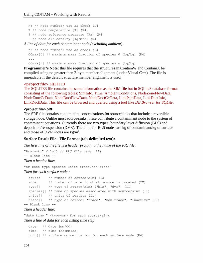
Using CONTAM – Working with Results
204
nr // node number; use as check (I4)
T // node temperature [K] (R4)
P // node reference pressure [Pa] (R4)
D // node air density [kg/m^3] (R4)
A line of data for each contaminant node (excluding ambient):
nr // node number; use as check (I4)
CCmax[0] // maximum mass fraction of species 0 [kg/kg] (R4)
...
CCmax[n] // maximum mass fraction of species n [kg/kg]
Programmer's Note: this file requires that the structures in ContamW and ContamX be
compiled using no greater than 2-byte member alignment (under Visual C++). The file is
unreadable if the default structure member alignment is used.
<project file>.SQLITE3 The SQLITE3 file contains the same information as the SIM file but in SQLite3 database format
consisting of the following tables: SimInfo, Time, AmbientConditions, NodeZoneFlowData,
NodeZoneCcData, NodeDuctFlowData, NodeDuctCcData, LinkPathData, LinkDuctInfo,
LinkDuctData. This file can be browsed and queried using a tool like DB Browser for SQLite.
<project file>.SRF The SRF file contains contaminant concentrations for source/sinks that include a reversible
storage node. Unlike most source/sinks, these contribute a contaminant node to the system of
contaminant equations. Currently there are two types: boundary layer diffusion (BLS) and
deposition/resuspension (DVR). The units for BLS nodes are kg of contaminant/kg of surface
and those of DVR nodes are kg/m2.
Surface Result File - File Format (tab-delimited text):
The first line of the file is a header providing the name of the PRJ file:
"Project:" file[] // PRJ file name (I1)
-- Blank line --
Then a header line:
"nr zone type species units trace/non-trace"
Then for each surface node :
source // number of source/sink (IX)
zone // number of zone in which source is located (IX)
type[] // type of source/sink ("bls", "dvr") (I1)
species[] // name of species associated with source/sink (I1)
units[] // units of results (I1)
trace[] // type of source: "trace", "non-trace", "inactive" (I1)
-- Blank line --
Then a header line:
"date time " <type+nr> for each source/sink
Then a line of data for each listing time step:
date // date (mm/dd)
time // time (hh:mm:ss)
conc[] // surface concentration for each surface node (R4)
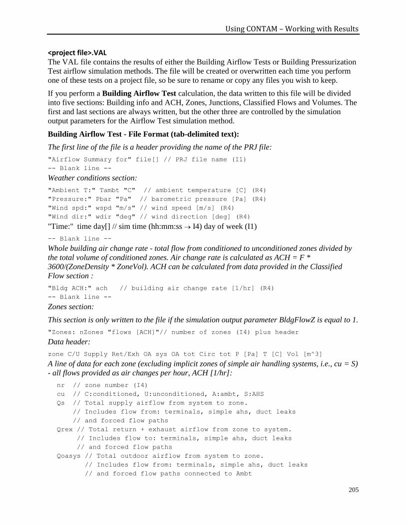
Using CONTAM – Working with Results
205
<project file>.VAL The VAL file contains the results of either the Building Airflow Tests or Building Pressurization
Test airflow simulation methods. The file will be created or overwritten each time you perform
one of these tests on a project file, so be sure to rename or copy any files you wish to keep.
If you perform a Building Airflow Test calculation, the data written to this file will be divided
into five sections: Building info and ACH, Zones, Junctions, Classified Flows and Volumes. The
first and last sections are always written, but the other three are controlled by the simulation
output parameters for the Airflow Test simulation method.
Building Airflow Test - File Format (tab-delimited text):
The first line of the file is a header providing the name of the PRJ file:
"Airflow Summary for" file[] // PRJ file name (I1)
-- Blank line --
Weather conditions section:
"Ambient T:" Tambt "C" // ambient temperature [C] (R4)
"Pressure:" Pbar "Pa" // barometric pressure [Pa] (R4)
"Wind spd:" wspd "m/s" // wind speed [m/s] (R4)
"Wind dir:" wdir "deg" // wind direction [deg] (R4)
"Time:" time day[] // sim time (hh:mm:ss I4) day of week (I1)
-- Blank line --
Whole building air change rate - total flow from conditioned to unconditioned zones divided by
the total volume of conditioned zones. Air change rate is calculated as ACH = F *
3600/(ZoneDensity * ZoneVol). ACH can be calculated from data provided in the Classified
Flow section :
"Bldg ACH:" ach // building air change rate [1/hr] (R4)
-- Blank line --
Zones section:
This section is only written to the file if the simulation output parameter BldgFlowZ is equal to 1.
"Zones: nZones "flows [ACH]"// number of zones (I4) plus header
Data header:
zone C/U Supply Ret/Exh OA sys OA tot Circ tot P [Pa] T [C] Vol [m^3]
A line of data for each zone (excluding implicit zones of simple air handling systems, i.e., cu = S)
- all flows provided as air changes per hour, ACH [1/hr]:
nr // zone number (I4)
cu // C:conditioned, U:unconditioned, A:ambt, S:AHS
Qs // Total supply airflow from system to zone.
// Includes flow from: terminals, simple ahs, duct leaks
// and forced flow paths
Qrex // Total return + exhaust airflow from zone to system.
// Includes flow to: terminals, simple ahs, duct leaks
// and forced flow paths
Qoasys // Total outdoor airflow from system to zone.
// Includes flow from: terminals, simple ahs, duct leaks
// and forced flow paths connected to Ambt
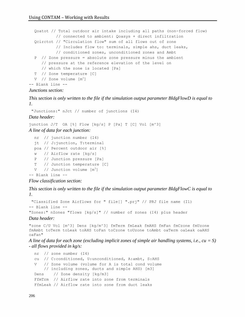
Using CONTAM – Working with Results
206
Qoatot // Total outdoor air intake including all paths (non-forced flow)
// connected to ambient: Qoasys + direct infiltration
Qcirctot // "Circulation flow" sum of all flows out of zone
// Includes flow to: terminals, simple ahs, duct leaks,
// conditioned zones, unconditioned zones and Ambt
P // Zone pressure = absolute zone pressure minus the ambient
// pressure at the reference elevation of the level on
// which the zone is located [Pa]
T // Zone temperature [C]
V // Zone volume [m3]
-- Blank line --
Junctions section:
This section is only written to the file if the simulation output parameter BldgFlowD is equal to
1.
"Junctions:" nJct // number of junctions (I4)
Data header:
junction J/T OA [%] Flow [kg/s] P [Pa] T [C] Vol [m^3]
A line of data for each junction:
nr // junction number (I4)
jt // J:junction, T:terminal
poa // Percent outdoor air [%]
w // Airflow rate [kg/s]
P // Junction pressure [Pa]
T // Junction temperature [C]
V // Junction volume [m3]
-- Blank line --
Flow classification section:
This section is only written to the file if the simulation output parameter BldgFlowC is equal to
1.
"Classified Zone Airflows for " file[] ".prj" // PRJ file name (I1)
-- Blank line --
"Zones:" nZones "flows [kg/s]" // number of zones (I4) plus header
Data header:
"zone C/U Vol [m^3] Dens [kg/m^3] fmTerm fmLeak fmAHS fmFan fmCzone fmUzone
fmAmbt toTerm toLeak toAHS toFan toCzone toUzone toAmbt oaTerm oaLeak oaAHS
oaFan"
A line of data for each zone (excluding implicit zones of simple air handling systems, i.e., cu = S)
- all flows provided in kg/s:
nr // zone number (I4)
cu // C:conditioned, U:unconditioned, A:ambt, S:AHS
V // Zone volume (volume for A is total cond volume
// including zones, ducts and simple AHS) [m3]
Dens // Zone density [kg/m3]
FfmTrm // Airflow rate into zone from terminals
FfmLeak // Airflow rate into zone from duct leaks
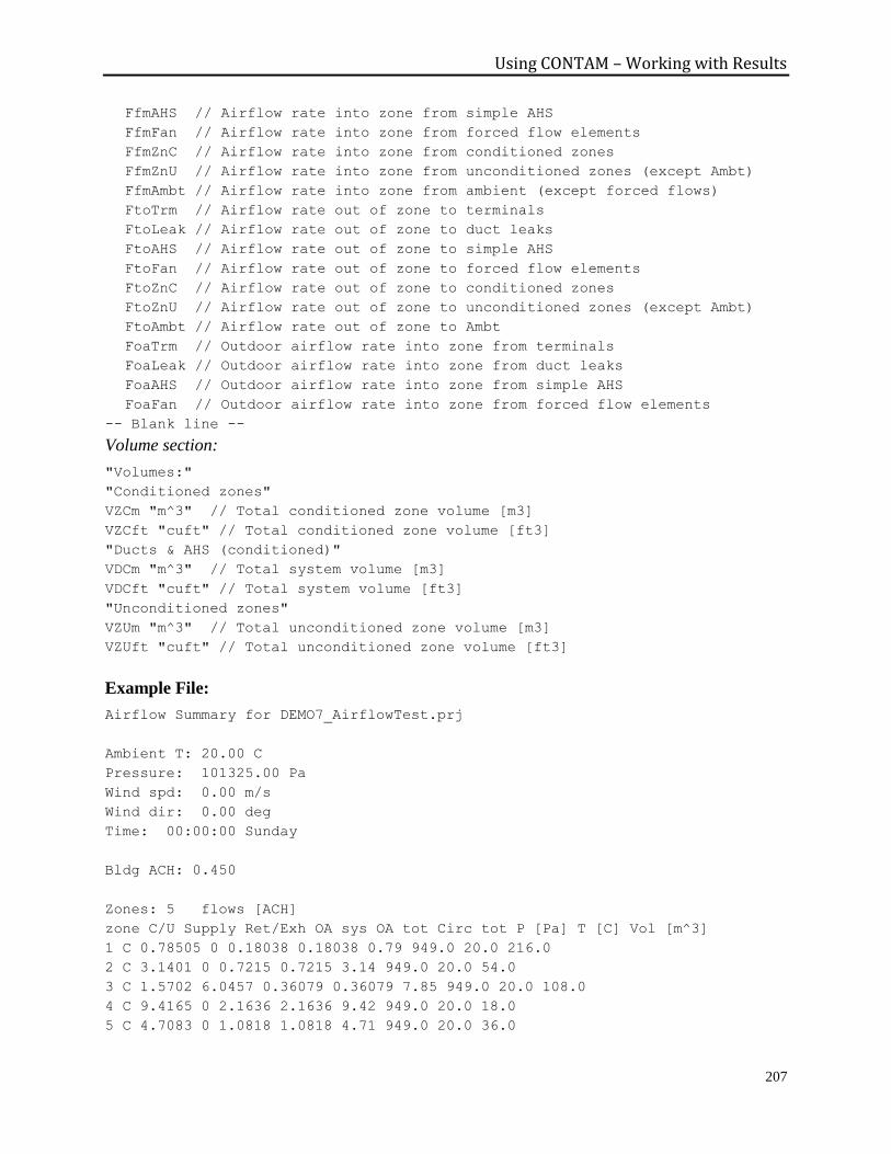
Using CONTAM – Working with Results
207
FfmAHS // Airflow rate into zone from simple AHS
FfmFan // Airflow rate into zone from forced flow elements
FfmZnC // Airflow rate into zone from conditioned zones
FfmZnU // Airflow rate into zone from unconditioned zones (except Ambt)
FfmAmbt // Airflow rate into zone from ambient (except forced flows)
FtoTrm // Airflow rate out of zone to terminals
FtoLeak // Airflow rate out of zone to duct leaks
FtoAHS // Airflow rate out of zone to simple AHS
FtoFan // Airflow rate out of zone to forced flow elements
FtoZnC // Airflow rate out of zone to conditioned zones
FtoZnU // Airflow rate out of zone to unconditioned zones (except Ambt)
FtoAmbt // Airflow rate out of zone to Ambt
FoaTrm // Outdoor airflow rate into zone from terminals
FoaLeak // Outdoor airflow rate into zone from duct leaks
FoaAHS // Outdoor airflow rate into zone from simple AHS
FoaFan // Outdoor airflow rate into zone from forced flow elements
-- Blank line --
Volume section:
"Volumes:"
"Conditioned zones"
VZCm "m^3" // Total conditioned zone volume [m3]
VZCft "cuft" // Total conditioned zone volume [ft3]
"Ducts & AHS (conditioned)"
VDCm "m^3" // Total system volume [m3]
VDCft "cuft" // Total system volume [ft3]
"Unconditioned zones"
VZUm "m^3" // Total unconditioned zone volume [m3]
VZUft "cuft" // Total unconditioned zone volume [ft3]
Example File:
Airflow Summary for DEMO7_AirflowTest.prj
Ambient T: 20.00 C
Pressure: 101325.00 Pa
Wind spd: 0.00 m/s
Wind dir: 0.00 deg
Time: 00:00:00 Sunday
Bldg ACH: 0.450
Zones: 5 flows [ACH]
zone C/U Supply Ret/Exh OA sys OA tot Circ tot P [Pa] T [C] Vol [m^3]
1 C 0.78505 0 0.18038 0.18038 0.79 949.0 20.0 216.0
2 C 3.1401 0 0.7215 0.7215 3.14 949.0 20.0 54.0
3 C 1.5702 6.0457 0.36079 0.36079 7.85 949.0 20.0 108.0
4 C 9.4165 0 2.1636 2.1636 9.42 949.0 20.0 18.0
5 C 4.7083 0 1.0818 1.0818 4.71 949.0 20.0 36.0
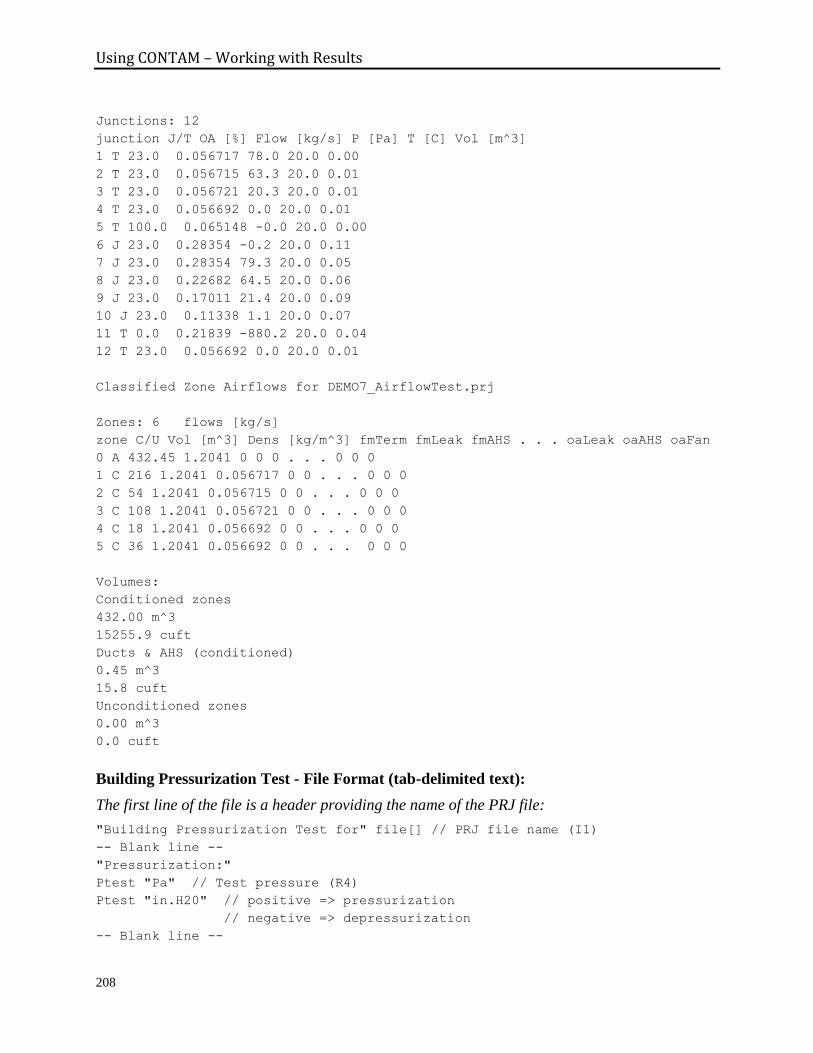
Using CONTAM – Working with Results
208
Junctions: 12
junction J/T OA [%] Flow [kg/s] P [Pa] T [C] Vol [m^3]
1 T 23.0 0.056717 78.0 20.0 0.00
2 T 23.0 0.056715 63.3 20.0 0.01
3 T 23.0 0.056721 20.3 20.0 0.01
4 T 23.0 0.056692 0.0 20.0 0.01
5 T 100.0 0.065148 -0.0 20.0 0.00
6 J 23.0 0.28354 -0.2 20.0 0.11
7 J 23.0 0.28354 79.3 20.0 0.05
8 J 23.0 0.22682 64.5 20.0 0.06
9 J 23.0 0.17011 21.4 20.0 0.09
10 J 23.0 0.11338 1.1 20.0 0.07
11 T 0.0 0.21839 -880.2 20.0 0.04
12 T 23.0 0.056692 0.0 20.0 0.01
Classified Zone Airflows for DEMO7_AirflowTest.prj
Zones: 6 flows [kg/s]
zone C/U Vol [m^3] Dens [kg/m^3] fmTerm fmLeak fmAHS . . . oaLeak oaAHS oaFan
0 A 432.45 1.2041 0 0 0 . . . 0 0 0
1 C 216 1.2041 0.056717 0 0 . . . 0 0 0
2 C 54 1.2041 0.056715 0 0 . . . 0 0 0
3 C 108 1.2041 0.056721 0 0 . . . 0 0 0
4 C 18 1.2041 0.056692 0 0 . . . 0 0 0
5 C 36 1.2041 0.056692 0 0 . . . 0 0 0
Volumes:
Conditioned zones
432.00 m^3
15255.9 cuft
Ducts & AHS (conditioned)
0.45 m^3
15.8 cuft
Unconditioned zones
0.00 m^3
0.0 cuft
Building Pressurization Test - File Format (tab-delimited text):
The first line of the file is a header providing the name of the PRJ file:
"Building Pressurization Test for" file[] // PRJ file name (I1)
-- Blank line --
"Pressurization:"
Ptest "Pa" // Test pressure (R4)
Ptest "in.H20" // positive => pressurization
// negative => depressurization
-- Blank line --

Using CONTAM – Working with Results
209
"Mass flow rate:"
F "kg/s" // Flow rate required to obtain Test pressure (R4)
F "kg/h"
F "scfm"
-- Blank line --
"Volume flow rate:"
Q "L/s" // Flow rate required to obtain Test pressure (R4)
Q "m^3/h"
Q "cfm"
-- Blank line --
"Ambient conditions:"
"Pressure"
Pambt "Pa" // Barometric pressure (R4)
Pambt "in.H2O"
"Temperature"
Tambt "C" // Outdoor temperature (R4)
Tambt "F"
"Air Density"
Dambt "kg/m^3" // Outdoor air density (R4)
Dambt "lb/ft^3"
-- Blank line --
"Volumes:"
"Conditioned zones"
VZC "m^3" // Total volume of conditioned zones
VZC "cuft"
"Ducts & AHS (conditioned)"
VD "m^3" // Total volume of ducts and AHS
VD "cuft"
"Unconditioned zones"
VZU "m^3" // Total volume of conditioned zones
VZU "cuft"
-- Blank line --
"Airflow details:"
"Path Czone Uzone dP [Pa] [in.H2O] F [kg/s] [kg/h] [scfm] Q [L/s] [m^3/h]
[cfm]"
A line of data for each flow path contains airflow details. All flows and pressure differences are
absolute values. If test is pressurization test, then all flows are from conditioned to
unconditioned zones. If a depressurization test, then flows are from unconditioned to conditioned
zones.
nr // path number
Czone // number of conditioned zone
Uzone // number of unconditioned zone
dP_Pa // pressure difference across path [Pa]
dP_iH20 // [in.H20]
F_kgs // mass flow through path [kg/s]
F_kgh // [kg/h]
F_scfm // [scfm]
Q_Ls // volume flow through path [L/s]
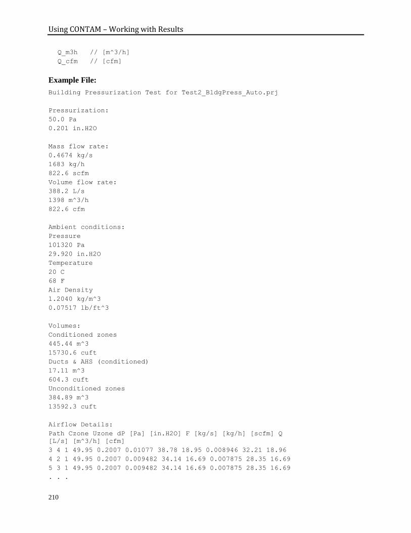
Using CONTAM – Working with Results
210
Q_m3h // [m^3/h]
Q_cfm // [cfm]
Example File:
Building Pressurization Test for Test2_BldgPress_Auto.prj
Pressurization:
50.0 Pa
0.201 in.H2O
Mass flow rate:
0.4674 kg/s
1683 kg/h
822.6 scfm
Volume flow rate:
388.2 L/s
1398 m^3/h
822.6 cfm
Ambient conditions:
Pressure
101320 Pa
29.920 in.H2O
Temperature
20 C
68 F
Air Density
1.2040 kg/m^3
0.07517 lb/ft^3
Volumes:
Conditioned zones
445.44 m^3
15730.6 cuft
Ducts & AHS (conditioned)
17.11 m^3
604.3 cuft
Unconditioned zones
384.89 m^3
13592.3 cuft
Airflow Details:
Path Czone Uzone dP [Pa] [in.H2O] F [kg/s] [kg/h] [scfm] Q
[L/s] [m^3/h] [cfm]
3 4 1 49.95 0.2007 0.01077 38.78 18.95 0.008946 32.21 18.96
4 2 1 49.95 0.2007 0.009482 34.14 16.69 0.007875 28.35 16.69
5 3 1 49.95 0.2007 0.009482 34.14 16.69 0.007875 28.35 16.69
. . .
Using CONTAM – Working with Results
211
205 16 0 50.00 0.2009 0.009616 34.62 16.92 0.007987 28.75 16.92
206 16 0 50.00 0.2009 0.001923 6.924 3.384 0.001597 5.75 3.385
<project name>.XLOG – ContamX LOG File The simulation engine will produce the text-based log file .XLOG within the same directory as
the PRJ file. This file mostly contains simulation performance data that is typically not relevant
to most users. However, if you encounter an error during simulation, this file can be useful to the
program developers in tracing the error.
3.19.2 Viewing Results
This section describes how to activate the results display mode of ContamW and to display the
results at different time-steps upon the SketchPad of transient simulations.
Results Display Mode To view results using ContamW you activate the results display mode by checking either the
SketchPad Results or the Results Display Window selection of the View menu. This will occur
automatically after the successful completion of a simulation or after opening a project file that
has simulation result files associated with it. Once the results display mode is activated, the
status bar will display result-related information (See Status Bar) and you will be able to utilize
all of the Results Display Methods outlined below.
Time Step If you have performed a transient simulation, results will be available for each time step.
However, the SketchPad results (as described in the following section) can only be displayed for
a single time-step at a time. You can change the time-step for which results are currently
displayed upon the SketchPad using the following menu and keyboard shortcut commands
available under the View → Results Navigation menu.
Show Next Time Step
Menu Command: Next Time Step
Keyboard Shortcut: End
Show Previous Time StepMenu Command: Previous Time Step
Keyboard Shortcut: Home
Show Last Time Step (of the day)
Menu Command: Last Time Step
Keyboard Shortcut: Ctrl+End
Show First Time Step (of the day)
Menu Command: First Time Step
Keyboard Shortcut: Ctrl+Home
The increment for the following "Jump" commands can be set via the Results Display properties
of the Project Configuration.
Jump Ahead (n time steps)
Menu Command: Jump Ahead
Keyboard Shortcut: Shift+End

Using CONTAM – Working with Results
212
Jump Back (n time steps)
Menu Command: Jump Back
Keyboard Shortcut: Shift+Home
Go to Date/Time…
Menu Command: Go to Date/Time
Keyboard Shortcut: Ctrl+G
3.19.3 Results Display Methods
This section describes the various methods that ContamW uses to present simulation results.
These methods include SketchPad for airflow paths, a Results Display Window for more detailed
information on the icon currently highlighted on the SketchPad, plotting transient results on
graphs, shaft reports, and exporting results to various types of external files. You can also print
copies of the graphs you view with ContamW or copy them to the Windows clipboard to be
pasted into other applications (e.g. word processor applications for written reports).
3.19.4 SketchPad Results
ContamW will display color-coded bars indicating the relative airflow rates and pressure drops
associated with each airflow path, duct terminal, or the supplies and returns of simple air-
handling systems for the current time-step on the current level of the SketchPad. By default,
Airflow rates are displayed with green lines and pressure differences with red lines. Display
colors are user-selectable (See Configuring ContamW). These result-bars will only appear if you
have selected the Airflows option on the Output page of the Simulation Parameters property
sheet. If you have set flow or pressure limits for a given airflow path (see Airflow Path
Properties), and they have been exceeded, the icon will be highlighted in red as a warning
indicator.
You can also highlight individual icons on the SketchPad to display results related to the specific
icon. Results can be viewed in the ContamW Status Bar and Floating Status Bar (See Status Bar
in the Getting Started section of the documentation). The following is a brief explanation of the
results displayed for each building component.
Airflow path – pressure difference, airflow rate and direction of pressure drop and airflow
Duct segment – pressure difference, airflow rate, velocity and direction of pressure drop
and airflow where velocity is calculated from the area of the duct segment
Simple air handling system – outdoor, recirculation and exhaust airflow rate
Supply and return of simple air handling system – airflow rate
Zone – zone temperature and reference pressure, i.e., the absolute pressure of the zone
relative to the absolute pressure of the ambient at the elevation of the level on which the
zone is located. Prior to CONTAM 2.4, this pressure was relative to the ambient pressure
at the reference elevation of the building. So now these pressures more closely resemble a
gage pressure.
Duct junction – junction temperature and static pressure relative to the pressure at the
height of the junction in the zone in which the junction is located

Using CONTAM – Working with Results
213
Duct terminal – airflow rate and velocity based on the terminal free face area, temperature
and static pressure relative to the pressure at the height of the terminal in the zone in which
the terminal is located
3.19.5 Results Display Window
The ContamW Results Display window displays different types of information depending on the
type of simulation that was performed (steady state or transient) the type of output that you
selected (see Output Properties) and the currently (or most recently) highlighted icon on the
SketchPad. The results display window will display information associated with zone icons and
exposure icons. Once in the results mode, you can control the visibility of the Results Display
window using the Results Display Window selection of the View menu. However, you can only
display the Results Display window while the SketchPad results are displayed.
For steady-state simulations the steady-state results will be displayed. For transient simulations,
results will be displayed for the current time step. Select the simulation time-step for which you
want results to be displayed using the Simulation Time Step commands outlined in the previous
section on Viewing Results.
Contaminant Concentration Results If the currently highlighted icon is a zone icon, then contaminant results will be displayed in the
Results Display Window. The concentration for each contaminant (species used in the
simulation) will be displayed in the units of the default concentration of each contaminant (See
Species Properties in the Working with Species and Contaminants section).
Zone Airflow Results If the currently highlighted icon is a zone icon, then for each adjacent zone the sum of the
airflows between the highlighted zone the adjacent zone will be displayed in the Default Units of
Flow set for the project (See Default Units in the Configuring ContamW section).
Exposure Results Summary exposure results are now available in the exposure box whisker (.EBW) file (See
Results Files).
3.19.6 Plotting Results
ContamW provides you with some charting features for plotting transient simulation results. You
can plot airflow, contaminant and exposure results using these features. Charting is only
available for transient simulation results of the currently loaded CONTAM project. You can plot
results for airflows and pressure differences, contaminant concentrations, and occupant exposure
and potential dosage. You access these charting features from the Simulation menu when in the
results mode.
NOTE: If you select a plot menu item when the ContamW caret is highlighting an icon, that
item will appear in the list of items to plot when the associated Chart Control dialog box is
displayed. This feature allows you to plot results for a particular item by highlighting it on the
SketchPad as opposed to finding it in the list of items to plot on the Chart Control dialog box.
Plotting Airflow Results Menu Command: Simulation → Plot Airflow Results…
Using CONTAM – Working with Results
214
Plot airflow and pressure difference results for airflow paths. You can plot two-way flow rates
for those flow paths that implement two-way airflow elements. If you select not to show two-
way flows, ContamW will plot the net flow rate for airflow paths that implement two-way
airflow elements.
Plotting Contaminant Results Menu Command: Simulation → Plot Contaminant Results…
Plot the time-history of contaminant concentrations of zones.
Plotting Exposure Results Menu Command: Simulation → Plot Exposure Results…
Plot the time-history of occupant exposure to contaminants.
Plotting Particle Results Menu Command: Simulation → Plot Particle Results…
Plot the time-history of the particle size distribution for a single zone.
Plotting Temperature Results Menu Command: Simulation → Plot Temperature Results…
Plot the time-history of temperatures for multiple zones/junctions. This feature is provided for
plotting temperature results as determined when performing coupled heat transfer calculations
with either TRNSYS or EnergyPlus.
Chart Control: Transient Airflow Results
Use this dialog box to control how transient airflow and pressure results are plotted.
Paths to Plot/Paths Available: The plotted data for each airflow element will appear as a
separate trace, the "Paths to Plot" lists the airflow elements that will be graphed. To add an item
to this list select the appropriate airflow element type (paths, ducts, or junctions), scroll through
the list of available elements or enter the element number directly if known, then press the "
Add" button. To remove an item from the Paths to Plot field select the zone to be deleted and
then press the "Remove" button.
Date(s) to Plot: This field allows the you to select the dates of data you wish to plot on the
graph. The available dates for the given simulation file are shown for your reference. You must
set the dates to fall within this range of dates. Enter dates in the following format:
MMMDD - the first 3 letters of the month and then the day of the month with or without
spaces
Data to Plot: You can plot airflow rates, pressure differences, or both. If you plot both airflow
and pressure difference, then ContamW will produce a graph with two vertical axis - one for
airflow and one for pressure difference. You can select the units of these axis using the "Airflow
Units" and "Pressure Units" drop-down combo boxes on this dialog box.
You can also show two-way flows for flow elements that utilize two-way flow models. If you
leave "Show two-way flows" unchecked, then ContamW will plot the net flow rate for all flow
paths. If you check "Show two-way flows," then a zero component will be plotted for all flow
paths that do not implement two-way models.
Using CONTAM – Working with Results
215
Comment for chart title: Enter a comment you want to appear at the top of the chart to help
distinguish various plots from one another.
Chart Control: Transient Contaminant Results
Use this dialog box to control how transient contaminant results are plotted.
Contaminant to Plot: This lists all the currently defined project contaminants. Select the
contaminant for which you want results plotted.
Moisture Units: If the contaminant to plot is "H2O," then this section will be activated to
provide the ability to plot moisture in units of mass fraction, humidity ratio, or % relative
humidity. Mass fraction is the same units in which all other contaminants are reported, i.e., mass
of contaminant per mass of air. Humidity ratio is in units of mass of water vapor per mass of dry
air, i.e., mass of air less the mass of water vapor. %RH will utilize the equations presented in
Chapter 6 of ASHRAE 2005 Fundamentals [ASHRAE 2005] to calculate the relative humidity
based upon the mass fraction of H2O, temperature and absolute pressure in each of the Zones to
Plot. If you select Mass Fraction or Humidity Ratio you can select from the set of units available
in the Units list. When plotting humidity ratio, you should only plot in units of kg/kg, g/kg or
lb/lb and not in volumetric units as the conversion will not be correct due to the assumed
standard air density in CONTAM’s conversion routines.
Zones to Plot/Zones Available: The plotted contaminant data for each zone will appear as a
separate trace, the "Zones to Plot" lists the zones that will be graphed. To add an item to this list
select the appropriate level and zone name from the drop down boxes in the Zones Available
field and then press the "Add" button. To remove an item from the Zones to Plot field first
select the zone to be deleted and then press the "Remove" button.
Date(s) to Plot: This field allows the user to plot the contaminant results from a specified date
range within the simulations results file. The available dates for the given simulation file are
given, the user provided date range must fall between these dates. The dates are entered in the
form: the first 3 letters of the month and then the day of the month with or without spaces.
Comment for chart title: Enter a comment you want to appear at the top of the chart to help
distinguish various plots from one another.
Chart Control: Transient Exposure Results
Use this dialog box to control how transient exposure results are plotted.
Occupant to Plot: This is a list of the occupants for which you want to plot exposure results.
Use the "Occupants Available" section to select occupants to add to this list and click the
"Add" button or highlight an occupant in this list and remove it using the "Remove" button.
Contaminant to Plot: This lists all the currently defined project contaminants. Select the
contaminant for which you want results plotted.
Date(s) to Plot: This field allows the user to plot the contaminant results from a specified date
range within the simulations results file. The available dates for the given simulation file are
given, the user provided date range must fall between these dates. The dates are entered in the
form: the first 3 letters of the month and then the day of the month with or without spaces.
Comment for chart title: Enter a comment you want to appear at the top of the chart to help
distinguish various plots from one another.
Using CONTAM – Working with Results
216
3.19.7 Exporting Results
ContamW provides you with the ability to export results to external files. You can either
generate report files or export files. Report files are text files that are formatted for ease of
reading. Export files are tab-delimited, so you can easily import them into a spreadsheet. This
feature provides you with greater charting flexibility as well as the ability to perform more
sophisticated data analysis of your simulation results. You access this feature of ContamW by
selecting Export Results… from the Simulation menu or use the F5 shortcut key when the
results-display mode is active. This will display the "Export Data" dialog box as described in the
following section.
Export Data
This section provides detailed descriptions of the specific properties associated with generating
result reports and exporting results to external files.
Transient Results:
Results available from/to: This shows the range of dates/times for which results are
available in the simulation results file (.SIM) of the latest simulation.
Export transient results from/to: Select the range for the data to be exported. Enter the date
as the first 3 letters of the month followed by the day of the month with or without spaces,
e.g., Jan01, followed by the time in the following format HH:MM:SS.
Airflow Data: Options for reporting/exporting airflow data. Airflow rates will be reported in the
Default Units of Flow as selected via the Project Configuration properties (See Configuring
ContamW).
Report airflows of all paths for date/time: Create a text file formatted for ease of reading
that lists the airflows and pressure differences for all paths, zone pressures and temperatures
at the selected date and time.
Export airflows of all zones for date/time: Create a tab-delimitted file containing a table of
the total airflows between each zone of the building. The leftmost column lists the level and
name of the zones from which airflows and the topmost row lists the level and names of the
zones into which air flows. Therefore, all airflows are listed as positive values.
Export transient flow for airflow path number: Create a tab-delimitted file listing all the
airflow data for a specific airflow path. Select the airflow path number(s) for which you want
to output the airflow and pressure drop data for the range of time you select in the "Export
transient results from/to" dates and times indicated above.
Export average transient flow for each zone between export result times: Create a tab-
delimitted file listing the average airflow rates between zones averaged over the range of
time you select in the "Export transient results from/to" dates and times indicated above.
Contaminant Concentration Data: Options for reporting and exporting contaminant results.
Concentrations will be reported in the units associated with the default concentration of each
species/contaminant (See Species Properties).
Report transient concentrations of all zones for date/time: Create a text file formatted for
ease of reading that lists the contaminant concentrations for all zones and contaminants at the
selected date and time.
Using CONTAM – Working with Results
217
Report transient concentrations of all zones: Create a text file formatted for ease of
reading that lists the contaminant concentrations for all zones at the selected date and time.
Export transient concentrations of all zones: Create a tab-delimitted file listing the
transient contaminant concentrations for all zones and contaminants for the range of time you
select in the "Export transient results from/to" dates and times indicated above.
Export transient concentrations for zone: Create a tab-delimitted file listing the transient
contaminant concentrations for each contaminant in the selected zone for the range of time
you select in the "Export transient results from/to" dates and times indicated above.
Shaft Report
CONTAM is well suited for the analysis of smoke control systems. Because of the importance of
shafts for some smoke control systems [Klote and Milke 2002, Klote, et al. 2012], ContamW
provides a special reporting feature for shafts.
Defining Shafts You define shafts during the drawing phase of project development by placing zone icons
directly below one another (in the same column and row) on adjacent levels of a building. If
there is a zone icon in the same position on the level above or below the current level, those
zones are part of the shaft when ContamW generates a shaft report. The shaft consists of zones
that exist on contiguous levels having a zone icon in the same location on the SketchPad.
You create the shaft report by selecting Generate Shaft Report from the Simulation menu.
This will display a dialog box prompting you to execute the following three steps to define the
shaft zone icon and primary and secondary flow paths associated with the shaft across which you
want ContamW to report the airflows and pressure drops. The zone icon would typically
represent a stairwell, and the primary flow path would typically represent a stairwell door.
Steps to select a shaft for a shaft report:
1) Left-click on the zone icon that defines the shaft
2) Left-click on the primary airflow path icon
3) Left-click on the secondary airflow path icon
NOTE: Click the right mouse button to cancel the shaft report generation process.
Once you have completed the above steps, the shaft report will be displayed in a dialog box. The
report will display pressure drop, airflow rates and direction of airflow on every level of the shaft
where there are airflow path icons in the same location on the SketchPad as that of the primary
and secondary airflow paths. You can use the Shaft Report dialog box to select the units in which
the airflow rate and pressure drops are reported, and you can save a copy of the report to a text
file.

Using CONTAM – Working with Project Annotations
218
3.20 WORKING WITH PROJECT ANNOTATIONS
Project Annotations and the Project Description provide you with simple project documentation
features.
Annotations
You simply place an annotation icon onto the SketchPad (see Drawing Building Component
Icons) and then use the icon definition procedure (see Defining Building Component Icons) to
edit the text for the annotation. Once you have defined the text associated with the annotation
icon, the text will appear in the status bar whenever you highlight the icon with the caret. You
can edit, delete, and move the icon as you would any other building component icon.
Project Description The project file description is provided to help you manage your project files. This description
will be available when you are opening project files from within ContamW (see Working with
Project Files).

Special Applications of CONTAM – Building Pressurization Test
219
4 SPECIAL APPLICATIONS OF CONTAM
This section includes instructions, or considerations, for using CONTAM to simulate several
different building features (e.g. atria, stairwells and chimneys) and perform special building
analysis such as fan pressurization. There are also available, several references that present the
application of CONTAM in various studies [Emmerich and Persily 1996 and 1998; Emmerich
and Nabinger 2000; Fang and Persily 1995; Musser and Yuill 1999; Musser 2000; Persily 1998;
Persily and Martin 2000; Persily and Ivy 2001]. Also, check the bibliography provided on the
NIST IAQ Analysis website http://www.bfrl.nist.gov/IAQanalysis/pubs.htm. Some documents
are available directly from the website.
4.1 BUILDING PRESSURIZATION TEST
The building pressurization test (sometimes referred to as fan pressurization or blower door test)
is a common way of determining the airtightness of a building envelope. Fan pressurization is
relatively quick and inexpensive and it characterizes building envelope airtightness independent
of weather conditions. In this procedure, a large fan or blower is mounted in a door or window
and induces a large and roughly uniform pressure difference across the building shell [ASHRAE
2005, p 27.12; ASTM 1999]. A common airtightness rating is the airflow rate at 50 Pa divided
by the building volume to give units of air changes per hour. CONTAM now provides an
automated method of performing the Building Pressurization Test (See Working with
Simulations), but there are also "manual" methods of performing this test presented below for
informational purposes.
You may wish to do a simulated pressurization test to determine the airtightness rating of your
idealized building. This is easily done by setting one of the zones on the zero elevation level to a
constant pressure of 50 Pa, running the simulation, and then observing the total airflow out of
that zone. (Don't forget flows to other building levels.) You could also define an airflow path
using a constant volume airflow element through which you can vary the airflow until you
achieve the desired level(s) of pressurization. Use standard m3/h flow units and divide by the
building volume to get the air change rate at 50 Pa. Alternatively, the flow rate at 4 Pa can be
converted to an effective leakage area (ELA) using equations in Chapter 27 of the 2005
ASHRAE Fundamentals Handbook [ASHRAE 2005]. Use the CONTAM results display to
check that the building has been properly pressurized by moving the cursor to each path on the
envelope to get the pressure drop reported in the status bar. You can use the report of all flows to
get a listing of all flow and pressure drops. The pressure difference (dP) across every path to the
ambient zone should be close to -50 Pa. The value is negative, because the report considers flow
and dP to the zone listed in the "zone" column from the zone in the "from" to be positive. All
flows are to the "from" zone.
The reported pressure drop across various flow paths will not be exactly 50 Pa because of density
effects. Minimize these differences by running all zones and ambient at the same (standard)
temperature and no wind. Differences in pressure due to elevation make it critical that the
constant pressure zone be on the level with zero elevation.
In a multizone building the effects of partitioning (internal walls and floors) usually are
significant. There are two solutions depending on the goal of the simulation. If the goal is only
to achieve a uniform pressure difference across the entire building shell, add a very large opening
Special Applications of CONTAM – Smoke Control Systems
220
across each partition. If the goal is to reproduce a field test, simulate the internal doors as being
open to get a relatively uniform pressure inside the building.
Prior to performing these tests, you should make a copy of the project file, so you do not have to
reverse the changes to restore the original project file.
4.2 SMOKE CONTROL SYSTEMS
For a stairwell pressurization system, you may want to record the pressurization flows by
creating a simple AHS model with supply points in the shaft. Make these supply points the
secondary path. You may use supply point icons aligned on every level with some or most of the
flows set to zero, or you may use icons only on those levels with a pressurization flow.
Alternatively, for shafts on an exterior wall of the building, you may wish to use the constant
flow rate path elements through the exterior wall to provide the pressurization air. This type of
flow path will also report the pressure difference between the shaft and ambient. You may want
to align these constant flow paths above the open doorway on the first level. For details on
viewing shaft reports see Working with Simulation Results in the Using ContamW section of the
manual.
4.3 SHAFTS
Buildings contain several architectural features which offer very low resistance to airflow
between building levels. These features include atria, elevator shafts, and stairwells. CONTAM
provides two ways of modeling such a low resistance path: the phantom zone and the low-
resistance (or large) opening. Select the most appropriate model based on how this path interacts
with the rest of the model.
This interaction can be understood by using three flow resistances in series to model a shaft
between two levels. There is a resistance to flow through the shaft and resistances representing
the paths (doors) connecting the shaft to the two different levels. Using the powerlaw
relationship, Q = C(P)0.5, and assuming C = 3.10 for the shaft, 1.55 for an open door, and 0.01
for a closed door, the following equivalent flow coefficients, Ce = ( 1/Ci2)-0.5, are computed for
four different assumptions:
1. both doors closed, ignore shaft resistance: Ce = 0.007070
2. both doors closed, include shaft resistance: Ce = 0.007066
3. both doors open, ignore shaft resistance: Ce = 1.096
4. both doors open, include shaft resistance: Ce = 0.984
Cases (1) and (2) show that when flow resistance is dominated by the closed doors, it is not
necessary to include the shaft flow resistance. Cases (3) and (4) show that when the resistances at
the (open) doors is of the same order as the shaft resistance, it is important to include the shaft
resistance in the model. For a quick estimate of relative flow coefficients, remember that the
flow coefficient is usually roughly proportional to the opening area.
4.3.1 Atria
If an atrium were modeled as individual zones on each level, the inter-level flow resistances
would be very low. A cursory comparison of the inter-level opening areas to the sum of all
openings from the atrium to other zones will usually indicate that an atrium should be modeled
Special Applications of CONTAM – Shafts
221
using phantom zones. This is done by placing a standard zone icon at the atrium's lowest level.
You use this zone icon to define the atrium temperature and total volume. You should ignore the
floor area of the normal zone icon that is used to define the atrium zone. Place a phantom zone
icon at all higher levels which contain parts of the atrium. A phantom zone icon indicates that the
region within the walls on this level are actually part of the zone on the level below the icon. If it
is necessary to have different temperature or contaminant concentrations at the different levels in
an atrium, then those levels must be modeled as normal zones connected by flow paths with very
large openings.
4.3.2 Stairwells
Data to describe the airflow characteristics of a stairwell in terms of an equivalent orifice is
provided in [Achakji and Tamura 1988]. This representation is very well suited to being
implemented by CONTAM, which allows you to create a powerlaw flow element from the
physical characteristics of the stairwell. Stairwell characteristics include the cross-sectional
(horizontal) area of the stairwell shaft, whether the fronts of the stair treads are open or closed,
and the number of people on the stairs. This last item might be important in an evacuation
scenario. Since the equivalent orifice area of the shaft is on the same order as it's cross-sectional
area, and this area is likely to be smaller than the sum of the areas of the doors entering the
stairwell, it is generally best to model a stairwell as individual zones on each level connected by
openings which have been defined using the CONTAM stairwell airflow element that
implements the Achakji/Tamura model.
4.3.3 Elevator Shafts
Elevator shafts (hoistways) will generally lie in some modeling regime that falls between
stairwells and atria. Measured data for the flow resistance of an elevator shaft have not yet been
identified. CONTAM provides a powerlaw flow element based on flow resistance from the
Darcy/ Colebrook model of a conduit or duct. A significant difference between an elevator shaft
and a stairwell is that the door between the shaft and the building is never fully open because,
when it is open, air must flow through openings in the elevator car to pass between the building
and the shaft. Table 6.1 of [Klote and Milke 2002] presents orifice areas for closed elevator
doors which tend to be fairly small compared to the cross-sectional area of the shaft, especially
for hoistways with multiple cars, so it is likely that the airflow in most elevator shafts can be
modeled with sufficient accuracy by phantom zones. However, it may be necessary to split the
shaft into several sections to achieve sufficient accuracy in modeling contaminant transport.
4.3.4 Chimneys
You can use a duct to create a simple chimney model. At its simplest this will involve only a
single duct connecting the inside of the building to the outside with the Darcy-Colebrook duct
element used to model the flow resistance of the chimney. The height of the duct terminal points
must reflect the height of the chimney and a special high temperature zone must be created
around the inside terminal point so that the proper stack effect will result. Be sure to allow an
appropriate low resistance path from this special zone to the rest of the building.
Working with TRNSYS
222
5 WORKING WITH TRNSYS
The CONTAM simulation engine, ContamX, can be controlled via a set of TCP/IP socket
communication messages. This enables CONTAM to be coupled with other simulation software.
This socket communication capability, or bridge mode, has been utilized to couple CONTAM
with TRNSYS (www.trnsys.com) to perform combined airflow and heat transfer simulations for
multizone buildings. More specifically, TRNSYS implements a Type56 multizone building heat
transfer module with which CONTAM can be "synchronized" to share inputs and outputs
between a Type56 and a CONTAM representation of a multizone building.
Historically, TRNSYS has implemented Type96 and Type97, which were based on the airflow
calculation capabilities of CONTAM and its predecessor program AIRNET [Walton 1989a].
These types only provided access to a subset of the airflow network calculations that
CONTAM/AIRNET were capable of performing. Further, the types did not support the
contaminant calculations that CONTAM was capable of performing. Therefore, a new Type98
has been developed that acts as a server to ContamX and provides communication and exchange
of information/data between Type56 and ContamX. This implementation method provides the
continued benefit of the full features of CONTAM as it evolves without requiring a
redevelopment of a new type as previously required with Type96/97. In order to enable this
coupling, new socket communications messages have been added. These are documented in
Appendix B.
This section provides an overview of how to implement the latest version of Type98 [Dols
2014a, Dols 2014b] . This implementation is currently limited to the so-called quasi-dynamic (or
ping-pong) method of coupling, whereby each analysis tool converges independently, as opposed
to the dynamic coupling (or onion) method whereby convergence is attained between the coupled
tools.
5.1 TRNSYS-CONTAM UTILITIES AND SETUP
Coupling between CONTAM and TRNSYS is further enabled using a set of NIST-developed
tools that facilitate the process of developing the CONTAM and TRNSYS building models to be
coupled and forming the connectivity between the inputs and outputs of the TRNSYS types.
These tools are available on the IAQanalysis website (www.bfrl.nist.gov/IAQanalysis/index.htm)
alongside of CONTAM. They are briefly described below along with instructions pertaining to
where these files should be located on your Windows system in order to work with TRNSYS. In
the file paths below, Trnsys\ refers to the directory into which TRNSYS was installed.
5.2 SOFTWARE COMPONENTS AND FILES
Type98<version>.dll – Type98 dynamic link library file developed to TRNSYS specifications.
It is the go-between that handles communication of TRNSYS commands and data to/from
ContamX. The “<version>” portion of the file name will depend on the versions of both
TRNSYS and CONTAM for which the Type was compiled, e.g., “_t17_c32” indicates the DLL
is compatible with TRNSYS version 17 and CONTAM version 3.2.
Copy to the Trnsys\Userlib\ReleaseDLLs directory.
ContamX3.exe – This is the calculation engine (solver) of the CONTAM program. It utilizes
socket communication to transfer commands and data between Type98. It is installed in the
CONTAM installation folder.
Working with TRNSYS
223
Copy to the Trnsys\Exe directory.
Type98.bmp – Type98 icon that can be associated with static-dynamic proformas created during
CONTAM-TRNSYS coupling method outlined below.
Copy to the Trnsys\Studio\Proformas\Utility\Calling External Programs\CONTAM directory.
This file is not critical, but usage is described in process below.
CONTAM3DExport.exe – This program enables the creation of a Trnsys3D file (.idf) by
extruding CONTAM project files that have been drawn to scale using the new pseudo-geometry
drawing features of ContamW.
An installer is provided by NIST, and the program can be accessed via the NIST folder of the
Windows Start Menu.
Type56-98Coupler.exe – This program enables the creation of a static-dynamic proforma file
(.tpf) based on CONTAM project files and TRNSYS Type56 building files as outlined in the
coupling process below.
An installer is provided by NIST, and the program can be accessed via the NIST folder of the
Windows Start Menu.
type98.log – This is a log file for Type98.
This file is created during a coupled simulation in the same folder as the associated PRJ file.
5.3 TRNSYS-CONTAM COUPLING PROCESS
The following outline and figure describe the process of coupling a CONTAM project via
Type98 with TRNSYS Type56. It covers the basic method, but not all the details required for all
possible coupling scenarios. You may need to implement scheduling, thermostatic control, etc.
between the two types that are not automatically implemented by this process. However, this
process does provide the connectivity between the zone airflows and temperatures. One should
ensure that the CONTAM project to be used is fully defined prior to implementing the following
coupling process, as it can be a bit cumbersome to modify significant features of the project once
the coupling has been established. For example, adding/removing zones will cause major issues
and require the coupling formation to be repeated. On the other hand, changing schedules, non-
coupled controls, or adjusting simulation parameters of CONTAM should not require
reformation of the coupling.
Automatic INPUTS to Type98
The coupling process below will automatically create TRNSYS INPUTS to Type98 for each
zone temperature as well as ambient conditions: dry bulb temperature, barometric pressure, wind
speed, and wind direction.
Manual INPUTS to Type98
To establish a manual INPUT, define a Constant control node in the CONTAM project file and
give it a name. This can be used in many ways, e.g., to control the fraction of the design airflow
rate of a supply point.
Automatic OUTPUTS from Type98
Each connection (which is made up of the sum of airflows) between two zones and between a
zone and ambient is included as an TRNSYS OUTPUT from Type98.
Working with TRNSYS
224
Manual OUTPUTS from Type98
To establish a manual OUTPUT, define a Signal Split control node in the CONTAM project and
give it a name.
Windows
To create a window for the purposes of thermal modeling via Type 56, define an airflow path
within the CONTAM project that utilizes a two-way airflow element having a name that contains
the word "wind". Place the airflow path icon on the wall where you would like the center of the
window to be located. Define the elevation of the bottom of the window via the airflow path
Reference Elevation and define the height and width of the window via the airflow element
properties. If you do not want any airflow through the window during the coupled simulation,
then set the path multiplier to zero. Upon export, the window will be created in the idf file
according to these properties. You must ensure that the windows are fully contained within the
wall and do not overlap each other.
The Coupling Process
1. Open/Create a project in ContamW sample project file name: [test.prj].
The CONTAM model should be drawn to scale using a scaling factor. Using the scaling
factor should result in 3D geometry for each zone that will produce a zone volume that
closely matches the zone volumes.
2. Open the CONTAM3DExport program.
a. Select the CONTAM project [test.prj]
b. Click the Save Trnsys3D IDF button
This will create a Trnsys3d compatible IDF file [test_T3D.idf]
c. (Optional) Edit the IDF file with Google SketchUp using the Trnsys3d plugin. For
example you may want to change the building to account for solar effects by
changing the shape of a zone, e.g., the slope of the roof or add shading elements.
You can also inspect the building model for problems with surfaces.
3. Open the TRNSYS SimulationStudio program
a. Select the File -> New menu command
b. Select 3D Building Project (multizone) and click Next >>
c. Select the idf file that was created in step 2 above [test_T3D.idf] and click Open. A
prompt will appear to create a BUI file. This will also create a TRNSYS 17 building
file [test_T3D.b17]. SimulationStudio will now display a Type56-based project in
the Assembly Window.
d. Save the TRNSYS project [test_T3D_imported.tpf]
e. Exit SimulationStudio
4. Open the Type56-98Coupler program
a. Select the CONTAM project file from step 1 above [test.prj].
b. Select the B17 file produced in step 3 above [test_T3D.b17] and click Open.
Working with TRNSYS
225
c. Click the Create Files button to create an updated building file, a proforma and a
variable exchange file. The updated building file [test_T3D_coupled.b17] has the
following additions: airflow connections between zones, infiltrations added to zones
with a connection to ambient, ventilation flows for duct terminals, AHS supply paths
and duct leaks and inputs for these airflows. The proforma [test_T3D_coupled.tmf]
is referred to as a dynamic-static proforma. It takes the place of the dynamic
proforma for the previous Type 97. This is likely to be replaced in the future with a
new dynamic proforma for Type 98. In the meantime, each project you create will
implement its own dynamic-static proforma. The variable exchange file
[test_T3D_coupled.vef] provides the list of variables to be used by Type98 to
coordinate the data exchange during the simulation.
5. Establish the new proforma for use with TRNSYS
a. Copy the proforma [test_T3D_coupled.tmf] to the following sub directory of the
Trnsys\ directory: Studio\Proformas\Utility\Calling External Programs\CONTAM\,
or you can create your own directory for your CONTAM proformas under the
Proformas directory.
b. Additionally, you can copy the Type98.bmp file located in the Trnsys\CONTAM\
directory and give it the same name as that of the proforma but leave the bmp
extension. This enables TRNSYS to display the new proforma in the Assembly Area
with the Type98 icon.
6. Open the TRNSYS SimulationStudio program
a. Open the tpf file that was created in step 3 above [test_T3D_imported.tpf]
b. Change the Type56 unit to use the new building file from step 4
[test_T3D_coupled.b17].
i. Double click the Type56 icon; select the External Files tab and Browse to
select the B17 file.
ii. The automatic OUTPUTS of Type98 should now be listed as INPUTS for
Type56 under the Inputs tab. These are the inter-zone airflows or connections
established for coupling. You should also see any manual outputs from
Type98 that you created using ContamW in the list of available INPUTS.
7. Add the project-specific Type98 proforma to the TRNSYS project
a. Select the newly created Type98 proforma [test_T3D_coupled.tmf] from the Direct
Access Toolbar and drag it onto the Assembly Area.
b. Edit the Type98 unit to set the PRJ and VEF file parameters to [test.prj] and
[test_T3D_coupled.vef] respectively.
c. The inputs and outputs listed in the VEF file [test_T3D_coupled.vef] should all be
available via the Variables window of the unit (accessed by double clicking the
icon).
8. Create a TRNSYS input deck file
Working with TRNSYS
226
a. The name of the deck file is determined by the Global Infos properties. You can
change the name via the Assembly -> Control cards… menu command, scroll down
to the Deck file name item and change the file name as desired. The default name is
default.dck, but you can change it to anything you like, e.g.,
[test_T3D_imported.dck].
b. Select the Calculate -> Create input file menu command to create the deck file.
9. Update the TRNSYS deck file using the Type56-98Coupler program.
a. Click the Select the deck file button and Open the deck file [test_T3D_imported.dck]
that was created in step 8.
b. If you closed the Type56-98Coupler program you also need to select the CONTAM
project file again.
c. Click the Change Deck Name button to set the name of the updated deck file
[test_T3D_coupled.dck].
d. Click the Save New Deck File button to create the new deck file. This deck file will
have the connections between Type56 and Type98 established.
10. Import the new deck file back into the TRNSYS project.
a. In Simulation Studio use the File -> Import TRNSYS Input File… menu command
to open the newly created coupled deck file [test_T3D_coupled.dck].
b. You should see the connections between Type56 and Type98 (test_T3D_coupled)
and the INPUTS and OUTPUTS will be connected. If a weather file type reader,
e.g., Type109 or Type15, is present, then that type will be coupled to Type98’s
ambient condition inputs. If there is more than one of these types then the first one
found in the deck file will be used. Type15 is given preference over Type109, so
Type15 will be coupled before any Type109. Be sure to select the proper file reader
type for the weather file format being used, e.g., Type15-3 for EPW files.
c. You can use the logging flag of the VEF file to provide various levels of details to
the Type98.log file that will be created in the same directory as the TRNSYS project
file. Set the value between 0 for no logging and 3 for detailed logging.
After following these steps you will have a TRNSYS project that has the temperature and flow
connections made between Type56 and Type98 and possibly ambient condition connections
between Type98 and Type15. You can then proceed with making any other desired connections,
e.g., manual inputs/outputs established as described above.
NOTE: To run a simulation, the time step and the beginning and ending dates must be the same
in both the CONTAM project file and the TRNSYS simulation control cards. ContamW can be
used to view/plot temperature results.
TRNSYS-CONTAM Coupling Diagram
The following diagram illustrates the coupling process and the relationships between the files
and software involved in the coupling process. This diagram is based on coupling the first
version of Type98 that was developed for coupling CONTAM 3.1. The method has been slightly
modified with the development of CONTAM 3.2 which utilizes the VEF file in place of the AIR
Working with TRNSYS
227
file. The VEF file can be generated using the Type56-98Coupler, and the content of this text file
is also provided below. The above TRNSYS-CONTAM coupling process also includes the use
of the VEF file.
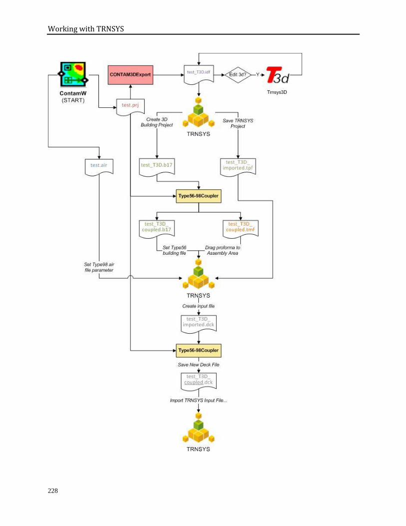
Working with TRNSYS
228
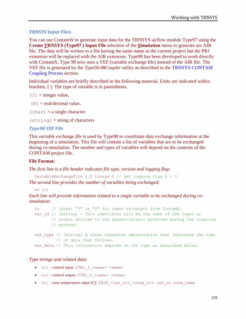
Working with TRNSYS
229
TRNSYS Input Files
You can use ContamW to generate input data for the TRNSYS airflow module Type97 using the
Create TRNSYS (Type97 ) Input File selection of the Simulation menu to generate ain AIR
file. The data will be written to a file having the same name as the current project but the PRJ
extension will be replaced with the AIR extension. Type98 has been developed to work directly
with ContamX. Type 98 now uses a VEF (variable exchange file) instead of the AIR file. The
VEF file is generated by the Type56-98Coupler utility as described in the TRNSYS CONTAM
Coupling Process section.
Individual variables are briefly described in the following material. Units are indicated within
brackets, [ ]. The type of variable is in parentheses.
(I) = integer value,
(R) = real/decimal value,
(char) = a single character
(string) = string of characters
Type98 VEF File
This variable exchange file is used by Type98 to coordinate data exchange information at the
beginning of a simulation. This file will contain a list of variables that are to be exchanged
during co-simulation. The number and types of variables will depend on the contents of the
CONTAM project file.
File Format:
The first line is a file header indicates file type, version and logging flag:
VariableExchangeFile 1.0 trnsys 0 // set logging flag 0 - 3
The second line provides the number of variables being exchanged:
nv (I)
Each line will provide information related to a single variable to be exchanged during co-
simulation:
io // (char) "I" or "O" for input to/output from ContamX.
var_id // (string) - This identifier will be the name of the input or
// output written to the dynamic/static proforma during the coupling
// process.
var_type // (string) A three character abbreviation that indicates the type
// of data that follows.
var_data // This information depends on the type as described below.
Type strings and related data:
cti – control input. CTRL_I_<name> <name>
cto – control output. CTRL_O_<name> <name>
zti – zone temperature input [C], TAIR_<lev_nr>_<zone_nr> lev_nr zone_name
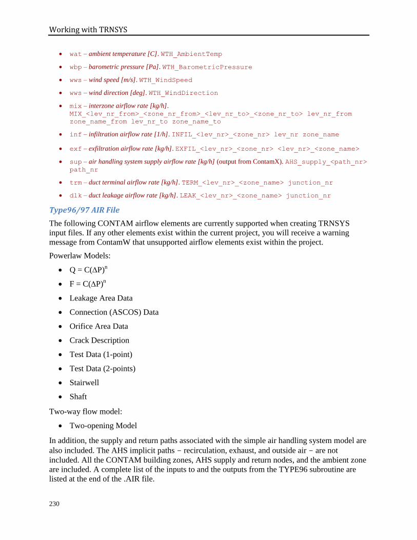
Working with TRNSYS
230
wat – ambient temperature [C]. WTH_AmbientTemp
wbp – barometric pressure [Pa]. WTH_BarometricPressure
wws – wind speed [m/s]. WTH_WindSpeed
wws – wind direction [deg]. WTH_WindDirection
mix – interzone airflow rate [kg/h].
MIX_<lev_nr_from>_<zone_nr_from>_<lev_nr_to>_<zone_nr_to> lev_nr_from
zone_name_from lev_nr_to zone_name_to
inf – infiltration airflow rate [1/h]. INFIL_<lev_nr>_<zone_nr> lev_nr zone_name
exf – exfiltration airflow rate [kg/h]. EXFIL_<lev_nr>_<zone_nr> <lev_nr>_<zone_name>
sup – air handling system supply airflow rate [kg/h] (output from ContamX). AHS_supply_<path_nr>
path_nr
trm – duct terminal airflow rate [kg/h]. TERM_<lev_nr>_<zone_name> junction_nr
dlk – duct leakage airflow rate [kg/h]. LEAK_<lev_nr>_<zone_name> junction_nr
Type96/97 AIR File
The following CONTAM airflow elements are currently supported when creating TRNSYS
input files. If any other elements exist within the current project, you will receive a warning
message from ContamW that unsupported airflow elements exist within the project.
Powerlaw Models:
Q = C(P)n
F = C(P)n
Leakage Area Data
Connection (ASCOS) Data
Orifice Area Data
Crack Description
Test Data (1-point)
Test Data (2-points)
Stairwell
Shaft
Two-way flow model:
Two-opening Model
In addition, the supply and return paths associated with the simple air handling system model are
also included. The AHS implicit paths - recirculation, exhaust, and outside air - are not
included. All the CONTAM building zones, AHS supply and return nodes, and the ambient zone
are included. A complete list of the inputs to and the outputs from the TYPE96 subroutine are
listed at the end of the .AIR file.
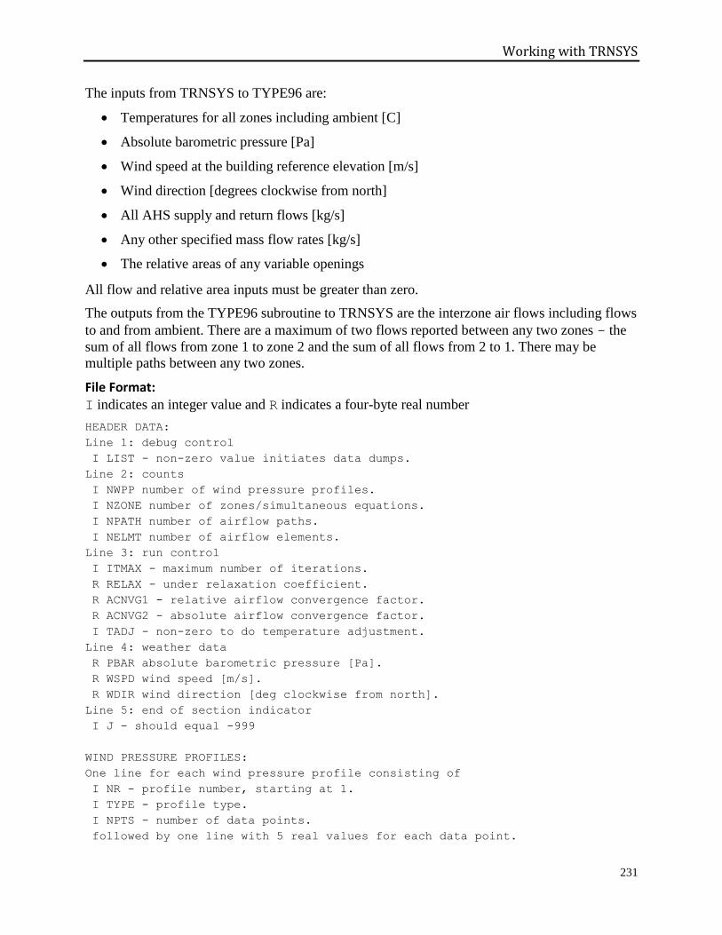
Working with TRNSYS
231
The inputs from TRNSYS to TYPE96 are:
Temperatures for all zones including ambient [C]
Absolute barometric pressure [Pa]
Wind speed at the building reference elevation [m/s]
Wind direction [degrees clockwise from north]
All AHS supply and return flows [kg/s]
Any other specified mass flow rates [kg/s]
The relative areas of any variable openings
All flow and relative area inputs must be greater than zero.
The outputs from the TYPE96 subroutine to TRNSYS are the interzone air flows including flows
to and from ambient. There are a maximum of two flows reported between any two zones - the
sum of all flows from zone 1 to zone 2 and the sum of all flows from 2 to 1. There may be
multiple paths between any two zones.
File Format: I indicates an integer value and R indicates a four-byte real number
HEADER DATA:
Line 1: debug control
I LIST - non-zero value initiates data dumps.
Line 2: counts
I NWPP number of wind pressure profiles.
I NZONE number of zones/simultaneous equations.
I NPATH number of airflow paths.
I NELMT number of airflow elements.
Line 3: run control
I ITMAX - maximum number of iterations.
R RELAX - under relaxation coefficient.
R ACNVG1 - relative airflow convergence factor.
R ACNVG2 - absolute airflow convergence factor.
I TADJ - non-zero to do temperature adjustment.
Line 4: weather data
R PBAR absolute barometric pressure [Pa].
R WSPD wind speed [m/s].
R WDIR wind direction [deg clockwise from north].
Line 5: end of section indicator
I J - should equal -999
WIND PRESSURE PROFILES:
One line for each wind pressure profile consisting of
I NR - profile number, starting at 1.
I TYPE - profile type.
I NPTS - number of data points.
followed by one line with 5 real values for each data point.
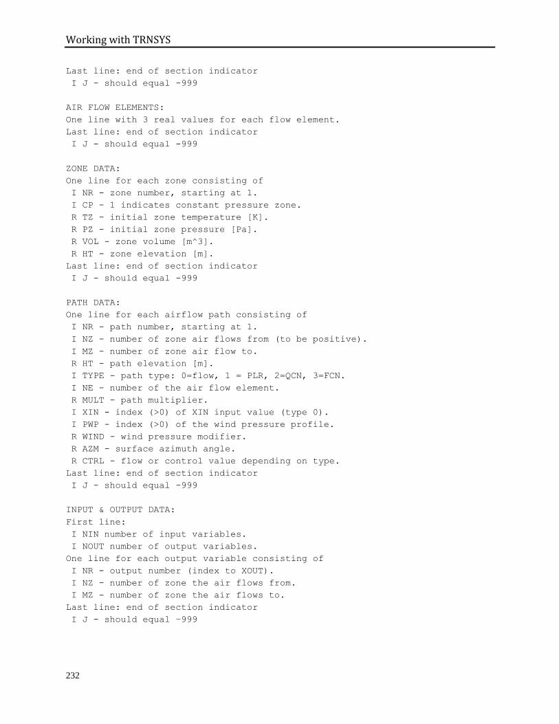
Working with TRNSYS
232
Last line: end of section indicator
I J - should equal -999
AIR FLOW ELEMENTS:
One line with 3 real values for each flow element.
Last line: end of section indicator
I J - should equal -999
ZONE DATA:
One line for each zone consisting of
I NR - zone number, starting at 1.
I CP - 1 indicates constant pressure zone.
R TZ - initial zone temperature [K].
R PZ - initial zone pressure [Pa].
R VOL - zone volume [m^3].
R HT - zone elevation [m].
Last line: end of section indicator
I J - should equal -999
PATH DATA:
One line for each airflow path consisting of
I NR - path number, starting at 1.
I NZ - number of zone air flows from (to be positive).
I MZ - number of zone air flow to.
R HT - path elevation [m].
I TYPE - path type: 0=flow, 1 = PLR, 2=QCN, 3=FCN.
I NE - number of the air flow element.
R MULT - path multiplier.
I XIN - index (>0) of XIN input value (type 0).
I PWP - index (>0) of the wind pressure profile.
R WIND - wind pressure modifier.
R AZM - surface azimuth angle.
R CTRL - flow or control value depending on type.
Last line: end of section indicator
I J - should equal -999
INPUT & OUTPUT DATA:
First line:
I NIN number of input variables.
I NOUT number of output variables.
One line for each output variable consisting of
I NR - output number (index to XOUT).
I NZ - number of zone the air flows from.
I MZ - number of zone the air flows to.
Last line: end of section indicator
I J - should equal –999
Working with EnergyPlus
233
6 WORKING WITH ENERGYPLUS
Beginning with CONTAM 3.2, ContamX can be coupled with EnergyPlus to perform combined
airflow and heat transfer simulations. This coupling is performed using CONTAM's previously
developed inter-process communication application programming interface (API). This API
consists of a set of socket communication messages that enable the control of execution and
exchange of data between ContamX and an external process. This same socket communication
capability, or bridge mode, has been previously utilized to couple CONTAM with TRNSYS
(www.trnsys.com) as documented in the Working with TRNSYS section. The socket
communication API is documented in Appendix B. Coupling between ContamX and
EnergyPlus is accomplished via co-simulation based on the Functional Mock-up Interface (FMI)
for Co-simulation specification version 1.0 [MODELISAR 2010]. EnergyPlus provides a master
algorithm that controls the simulation [DOE 2013, Nouidui et al. 2014, Wetter 2011], and a
newly developed module (ContamFMU.dll) is incorporated into a Functional Mock-up Unit
(FMU) for use during execution.
EnergyPlus sets up the dynamic data exchange between itself and the slave FMU based on the
co-simulation description file. Currently, the following data can be exchanged between
EnergyPlus and ContamX:
From EnergyPlus to ContamX
o Zone Temperatures
o Ventilation system airflow rates for zone supply and return airflow rates
o Outdoor airflow fractions of outdoor airflow controllers
o Exhaust fan airflow rates
o Energy recovery fan airflow rates
o Outdoor environment data including temperature, barometric pressure, wind speed
and wind direction obtained from EnergyPlus weather (.epw) files
o Output variables which may be EnergyPlus Output:Variable or
EnergyManagementSystem:OutputVariable objects
From ContamX to EnergyPlus
o Zone infiltration airflow rates
o Inter-zone airflow rates via airflow paths, i.e., not via ducts
o Controls values which may be any value exposed via a named “split” type control
node in a CONTAM controls network, e.g., a signal calling for ventilation airflow
due to an elevated contaminant level
The CONTAM3DExporter tool was developed by NIST to assist in the coupling between
CONTAM and EnergyPlus. This tool reads a CONTAM PRJ file and creates an IDF file that
contains objects associated with the geometry, infiltration and inter-zone mixing flows, an air
loop that includes an outdoor air mixer and HVAC airflow terminal, and FMI-related entities
required to facilitate dynamic data exchange. Detailed mappings between CONTAM and
EnergyPlus entities are provided in the table below. Items in the table with fixed-width fonts,
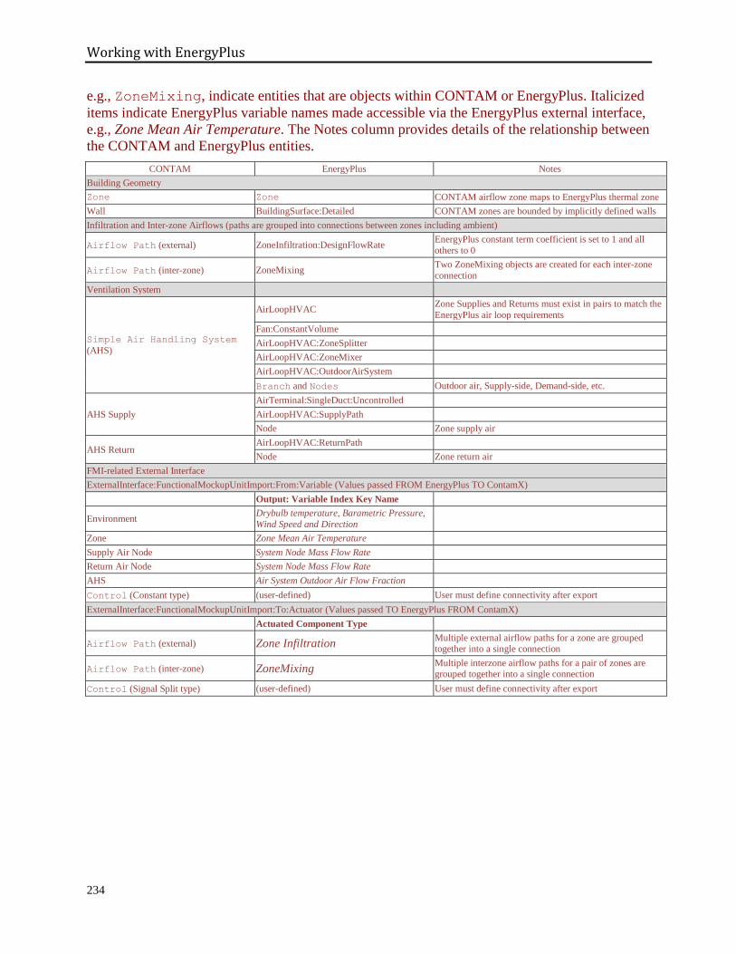
Working with EnergyPlus
234
e.g., ZoneMixing, indicate entities that are objects within CONTAM or EnergyPlus. Italicized
items indicate EnergyPlus variable names made accessible via the EnergyPlus external interface,
e.g., Zone Mean Air Temperature. The Notes column provides details of the relationship between
the CONTAM and EnergyPlus entities.
CONTAM EnergyPlus Notes
Building Geometry
Zone Zone CONTAM airflow zone maps to EnergyPlus thermal zone
Wall BuildingSurface:Detailed CONTAM zones are bounded by implicitly defined walls
Infiltration and Inter-zone Airflows (paths are grouped into connections between zones including ambient)
Airflow Path (external) ZoneInfiltration:DesignFlowRate EnergyPlus constant term coefficient is set to 1 and all
others to 0
Airflow Path (inter-zone) ZoneMixing Two ZoneMixing objects are created for each inter-zone
connection
Ventilation System
Simple Air Handling System
(AHS)
AirLoopHVAC Zone Supplies and Returns must exist in pairs to match the
EnergyPlus air loop requirements
Fan:ConstantVolume
AirLoopHVAC:ZoneSplitter
AirLoopHVAC:ZoneMixer
AirLoopHVAC:OutdoorAirSystem
Branch and Nodes Outdoor air, Supply-side, Demand-side, etc.
AHS Supply
AirTerminal:SingleDuct:Uncontrolled
AirLoopHVAC:SupplyPath
Node Zone supply air
AHS Return AirLoopHVAC:ReturnPath
Node Zone return air
FMI-related External Interface
ExternalInterface:FunctionalMockupUnitImport:From:Variable (Values passed FROM EnergyPlus TO ContamX)
Output: Variable Index Key Name
Environment Drybulb temperature, Barametric Pressure,
Wind Speed and Direction
Zone Zone Mean Air Temperature
Supply Air Node System Node Mass Flow Rate
Return Air Node System Node Mass Flow Rate
AHS Air System Outdoor Air Flow Fraction
Control (Constant type) (user-defined) User must define connectivity after export
ExternalInterface:FunctionalMockupUnitImport:To:Actuator (Values passed TO EnergyPlus FROM ContamX)
Actuated Component Type
Airflow Path (external) Zone Infiltration Multiple external airflow paths for a zone are grouped together into a single connection
Airflow Path (inter-zone) ZoneMixing Multiple interzone airflow paths for a pair of zones are grouped together into a single connection
Control (Signal Split type) (user-defined) User must define connectivity after export
Working with EnergyPlus
235
6.1 ENERGYPLUS-CONTAM COUPLING PROCESS
The following outline describes the process of coupling a CONTAM project with EnergyPlus. It
covers the basic method, but not all the details required for all possible coupling scenarios. This
process utilizes the CONTAM3DExport tool (referred to as the exporter) to generate an
EnergyPlus IDF file from a CONTAM PRJ file.
It is not absolutely necessary to follow this process in order to develop a coupled project. One
could develop a CONTAM project with corresponding thermal zones to an existing EnergyPlus
IDF, generate an IDF file with the CONTAM3DExport tool, and merge parts of the generated
IDF file into the EnergyPlus IDF file. However, coupling without this procedure will require care
in providing subsurfaces to contain individual flow paths of the associated CONTAM project.
Also, air loops and nodes of the generated and EnergyPlus IDF files will need to be coordinated.
Create the CONTAM Project using ContamW Use the following guidelines when creating your CONTAM project to be coupled with
EnergyPlus. The table in the Working with EnergyPlus section shows the objects created in the
EnergyPlus model and the corresponding CONTAM entities.
Geometry Utilize the pseudo-geometry mode of ContamW in order for CONTAM3DExport to generate the
necessary geometry of the EnergyPlus model. For each zone in the CONTAM model a thermal
zone will be created in the EnergyPlus model.
Airflow Paths Airflow paths will be grouped to form inter-zone mixing and infiltration airflow rates in the
EnergyPlus model.
Windows To create a window for the purposes of thermal modeling via EnergyPlus, define an airflow path
within the CONTAM project that utilizes a two-way airflow element having a name that contains
the character string "wind" (not case-sensitive). Place the airflow path icon on the wall where
you would like the center of the window to be located. Define the elevation of the bottom of the
window via the airflow path Reference Elevation, and define the height and width of the window
via the airflow element properties. If you do not want any airflow through the window during the
coupled simulation, then set the path multiplier to zero. Upon export, the window will be created
in the IDF file according to these properties. You must ensure that the windows are fully
contained within the wall and do not overlap each other.
Simple Air Handling Systems An air loop will be created in the EnergyPlus model for each simple air-handling system (AHS)
in the CONTAM model except as noted below for the exhaust-only and heat recovery ventilator
(HRV) systems. In order to adhere to the EnergyPlus air loop paradigm, each thermal zone that is
served by the air loop should have corresponding supply and return air terminals served by the
associated "normal" simple AHS in the CONTAM building model. A zone can only be served by
one air loop, so no more than one normal AHS should serve a zone in CONTAM. However, a
zone can be served by one of each type of AHS: normal, exhaust-only and HRV; as described
below.
Simple AHSs in CONTAM can be made to correspond to exhaust-only and energy recovery
systems in EnergyPlus. The name of the simple AHS is used to trigger CONTAM3DExport to
Working with EnergyPlus
236
create these systems along with system-specific supply and return terminal requirements.
Exhaust-only system names must contain "exh" (not case-sensitive), and should not have any
supply air terminals associated with them. Energy recovery system names should contain "hrv"
(not case-sensitive) and should not have any return air terminals associated with them.
CONTAM3DExport will perform checks on the PRJ file for these requirements. The exhaust-
only and hrv simple AHSs do not have corresponding air loops associated with them in
EnergyPlus. Instead, hrv systems will generate a
ZoneHVAC:EnergyRecoveryVentilator and associated objects in the IDF file, and the
exhaust-only system will generate a Fan:ZoneExhaust and associated objects in the IDF file.
Ducts Ducts are currently not supported when coupling with EnergyPlus. CONTAM3DExport will not
perform a check on this.
Controls In CONTAM Constant (or Set) type controls having a name are used to receive input control
signals from EnergyPlus. Split (or Pass) type controls having a name are used to send output
signals to EnergyPlus from CONTAM. Prior to executing a simulation with a project that has
controls, be sure to either run a CONTAM only simulation or at least a full building check via
the Simulation->Run Building Check menu item to make sure that the controls are sequenced.
This procedure must be followed after any new controls are added to a project, and the project
must also be saved after the controls are sequenced.
An ExternalInterface:FunctionalMockupUnitImport:From:Variable
object will be created for named Constant type controls, and an
ExternalInterface:FunctionalMockupUnitImport:To:Actuator object will
be created for named Split type controls. However, the user must set the Name property as well
as the Output:Variable and Actuated Component properties of the From:Variable and
To:Actuator objects respectively, directly within the IDF file after it has been created. The
To:Actuator object can be replaced with either a To:Schedule or To:Variable object
within the generated IDF file if desired.
Create the EnergyPlus IDF File using CONTAM3DExport
1. Run CONTAM3DExport and select the PRJ file to convert to EnergyPlus.
2. Select an existing IDF file that contains the Material and Construction objects that
you want to incorporate into the new IDF file.
3. Select which constructions you want to associate with each surface category.
4. Select the Building Coupled with CONTAM Export Option.
5. Click the Save EnergyPlus IDF button. You will be prompted when the export is complete.
Files Created by CONTAM3DExport
IDF file - contains the geometry, air loops, exhaust fans and FMU-related objects.
ContamFMU.fmu - a compressed zip file that will be unpacked and used during a
coupled EnergyPlus/CONTAM simulation. It contains the following files:
Working with EnergyPlus
237
o modelDescription.xml - used by the EnergyPlus FMI co-simulation master
algorithm to obtain data exchange parameters.
o contam.prj - the CONTAM project file used to generate the corresponding
EnergyPlus IDF file and used by ContamX during the co-simulation.
o contam.vef - used by ContamX to obtain data exchange parameters.
o ContamFMU.dll - dynamic link library utilized by the EnergyPlus master algorithm
to implement FMI-based program control and data exchange with ContamX.
o contamx3.exe - the CONTAM simulation engine controlled by the EnergyPlus FMI
co-simulation master algorithm via the ContamFMU.dll.
Modify IDF File The IDF file generated by CONTAM3DExport contains the building geometry, surface materials
and constructions, air loops, exhaust fans and partial external interface objects as described
above. However, the file will not include the HVAC components associated with the generation
or removal of energy, e.g., heating/cooling coils, internal gains, and thermostats. The IDF file
can now be edited using the IDF Editor or other text-based editor to add the desired HVAC
system components. The IDF file can also be viewed and edited using tools such as SketchUp
with the OpenStudio plug-in [Gugliemetti 2011, NREL 2015]. This is useful to modify the
rectangular elements that are created by CONTAM3DExport, for example to modify roofs to
have sloped surfaces and to add shading components to the building.
Run the Simulation The IDF file and ContamFMU.fmu file must be located in the same directory. The files in the
ContamFMU.fmu file can be extracted using a zip file decompression program. This may be
necessary to modify run control parameters of the contam.prj file as outlined below.
1. Set the time step and the beginning and ending dates to be the same in the contam.prj file
located in the ContamFMU.fmu file and the EnergyPlus IDF file.
2. Prior to running the coupled simulation, copy the contam.prj and contamx3.exe files from
the ContamFMU.fmu file into another directory. Using ContamW, open the contam.prj file
and set the simulation run control parameters to run a simulation for a single day that
corresponds to the first day of the desired coupled simulation. Run the simulation, and it
will generate a CONTAM restart file having the same name as the project file, i.e.,
contam.rst. Copy the RST file back to the original directory that contains the IDF and PRJ
files for the co-simulation. This restart file will be used by ContamX during the warm-up
period of the EnergyPlus simulations.
3. Use EPLaunch to select the IDF file and desired EnergyPlus weather (EPW) file and run
the simulation.
4. Once the simulation is complete, ContamW can be used to view/plot results of contam.prj
including temperatures.

Working with EnergyPlus
238
6.2 ENERGYPLUS INPUT FILES
These input files are utilized for the coupling process to coordinate the transfer of data during the
co-simulation between EnergyPlus and CONTAM via the ContamFMU.dll. These files can be
created using the CONTAM3DExportTool, but their contents are provided here.
contam.vef
This variable exchange file is used by ContamFMU.dll to coordinate data exchange information
at the beginning of a co-simulation run. This file will contain a list of variables that are to be
exchanged during co-simulation. The number and types of variables will depend on the contents
of the CONTAM project file.
In the following material individual variables are briefly described. Units are indicated within
brackets, [ ]. The type of variable is in parentheses.
(I) = integer value,
(R) = real/decimal value,
(char) = single character
(string) = string of characters
File Format: The first line is a file header indicates file type and version:
VariableExchangeFile 1.0
The second line provides the number of variables being exchanged:
nvariables (I)
Each line will provide information related to a single variable to be exchanged during co-
simulation:
input/output indicator // (char) “I” for input to ContamX or “O” for output
// to ContamX.
variable identification // (string) - This identifier is used to ensure the
// variables match those of the modelDescription.xml file. The order of
// these variables must match those in the xml file to ensure that
// EnergyPlus (the FMI master algorithm)can match the inputs and outputs
// with the slave process, ContamFMU.dll
variable type // (string) A three character abbreviation that indicates the
// type of data that follows.
variable data // This information depends on the type as described below.
Type strings and related data (for both FMI and Type98):
cti – control input. CTRL_I_<name> <name>
cto – control output. CTRL_O_<name> <name>
zti – zone temperature input [C], TAIR_<lev_nr>_<zone_name> lev_nr zone_name
wat – ambient temperature [C]. WTH_AmbientTemp
wbp – barometric pressure [Pa]. WTH_BarometricPressure
wws – wind speed [m/s]. WTH_WindSpeed
Working with EnergyPlus
239
wws – wind direction [deg]. WTH_WindDirection
mix – interzone airflow rate [m3/s]. MIX_<lev_from>_<zone_from>_<lev_to>_<zone_to>
lev_from zone_from lev_to zone_to
inf – infiltration airflow rate [m3/s]. INFIL_<lev_nr>_<zone_name> lev_nr zone_name
ahs – air handling system supply air terminal [m3/s] (input to ContamX).
AHS_supply_<lev_nr>_<zone_name> lev_nr zone_name ahs_nr
number_of_zones_served
ahr – air handling system supply air terminal (input to ContamX).
AHS_supply_<lev_nr>_<zone_name> lev_nr zone_name ahs_nr
number_of_zones_served
exh – exhaust-only air handling system return air terminal (input to ContamX).
AHS_exhaust_<lev_nr>_<zone_name> lev_nr zone_name ahs_nr
number_of_zones_served
hvs – energy recovery ventilator air handling system supply air terminal (input to ContamX).
AHS_supply_<lev_nr>_<zone_name> lev_nr zone_name ahs_nr
number_of_zones_served
hvr – energy recovery ventilator air handling system return air terminal (input to ContamX).
AHS_supply_<lev_nr>_<zone_name> lev_nr zone_name ahs_nr
number_of_zones_served
poa – air handling system percent outdoor air (input to ContamX). PCTOA_<AHS_name> ahs_name
modelDescription.xml
This file is used by the EnergyPlus co-simulation master algorithm to coordinate data exchange.
The general requirements of its content is defined by the FMI for co-simulation specification
[MODELISAR 2010a, MODELISAR 2010b]. The unique variable names are the same as those
provided for the <project>.vef, e.g., TAIR_<lev_nr>_<zone_name>.

Working with EnergyPlus
240
6.3 GETTING HELP
This help manual is available in both printed form and accompanying the ContamW program as
"on-line" help. There are several ways to access the on-line help system. You can either use the
Help Contents… selection of the Help menu to display the contents of the help manual or use
the context-sensitive feature to access help.
Help Contents You can browse the contents or index of the help system to view the topic of your choice and use
the search feature to display a list of help topics that contain the keyword in which you are
interested.
Context-Sensitive Help The context-sensitive help feature is designed to provide you with specific information related to
the currently active ContamW window or dialog box. To activate the context-sensitive help
system, press the F1 key.
Help Index and Search Be sure to use the on-line help index and search features if you are having trouble locating a
specific topic.
Obtaining Technical Support If you need to contact the CONTAM developers for guidance on using the program or to report a
technical problem with the program you can do so via email at the addresses below. If you
encounter an error while working with CONTAM, and you require assistance solving the
problem, you should immediately (before running ContamW or ContamX again) make copies of
the CONTAMW2.LOG, PROJECT.BKP and WEATHER.BKP located in the ContamW
application data directory (C:\Documents and Settings\<User Account>\Application
Data\NIST\ContamW\) and the .XLOG file located alongside the PRJ file. You can email these
files to NIST so that we may be better equipped to address your particular problem.
NIST Contact Information
IAQ and Ventilation Group 301-975-6431

Theoretical Background – Model Assumptions
241
7 THEORETICAL BACKGROUND
This section provides theoretical background of the CONTAM program. There are basically
three subsections: the first provides a summary of underlying assumptions of the model and the
others address the contaminant and airflow analysis respectively.
7.1 MODEL ASSUMPTIONS
CONTAM is a powerful tool that models airflow and contaminant dispersal in buildings. It is
important to realize that this tool implements mathematical relationships to model airflow and
contaminant related phenomenon and therefore incorporates assumptions that simplify the model
from that of the modeled phenomenon. The following is a brief description of these modeling
assumptions.
Well-mixed zones – This assumption refers to the treatment of each zone as a single node,
wherein the air has uniform (well-mixed) conditions throughout. These conditions include
temperature, pressure and contaminant concentrations. Therefore, localized effects within a
given zone cannot be accounted for using CONTAM. For example, if you utilize a contaminant
source that introduces a mass of contaminant into a zone at a certain time (burst source), the
contaminant will be diluted to the entire volume of the zone within a single time step.
One-Dimensional Convection/Diffusion Zones – In versions prior to CONTAM 2.3 all zones
were considered to be well-mixed, i.e., having a uniform concentration. However, beginning with
version 2.3, zones can be preconfigured by the user to be one-dimensional convection/diffusion
zones in which contaminants can be allowed to vary along a user-defined axis. When operating
under the newly added short time step method ContamX will provide for the ability of
contaminant concentration gradients to occur in the direction of the convection/diffusion axis by
programatically sub-dividing the zone into a series of well-mixed cells along the axis.
Duct Systems – Typically, during contaminant simulation, there are similarities between duct
junctions and well-mixed zones and between duct segments and airflow paths. In this case the
volumes of the duct junctions are determined from the duct segments to which they are
connected. However, in CONTAM 2.4 the entire duct system can modeled to account for one-
dimensional convection/diffusion flow through the system. This feature is available as an option
under the new short time step contaminant simulation method.
Conservation of mass – When performing a steady-state simulation, the mass of air within each
zone is conserved by the model. This implies that air can neither be created nor destroyed within
a zone. However, when performing a transient simulation, CONTAM now provides the option of
allowing the accumulation or reduction of mass within a zone due to the variation of zone
density/pressure and the implementation of non-trace contaminants within a simulation. This is
further addressed in this Theory section (see Airflow Analysis and Contaminant Analysis), as
well as in a previous section addressing simulation settings (see Airflow Numerics Properties).
Trace contaminants – Trace contaminants are those that are found in low enough levels that they
do not affect the density of air within a zone. You must be careful not to rely on the model to
handle contaminant concentrations that would cause a change in the density of air. The program
will allow for contaminants to reach levels that would, in actuality, affect the density, but the
program will still treat them as if they were trace contaminants.
Theoretical Background – Model Assumptions
242
Non-trace contaminants – Non-trace contaminants are those that are present in such quantities
that they can influence the air density, e.g., water vapor. In CONTAM you define those
contaminants that are components of the air within the building. CONTAM will treat them as a
mixture of ideal gases.
Thermal effects – The model does not handle heat transfer phenomenon per se, but does provide
for the scheduling of zone temperatures. Zone temperatures can be either constant or allowed to
change during transient simulations according to user-defined temperature schedules. CONTAM
will determine airflows and non-trace contaminant mass fractions induced by temperature
differences between zones including ambient (e.g., as caused by the stack effect). You can also
vary the outdoor temperature for transient simulations using weather files.
Airflow paths – Airflow through various airflow elements provided by CONTAM is modeled
using either a powerlaw or quadratic relationship between airflow and pressure difference across
the flow path. These relationships are models themselves, and care should be taken when
implementing them to represent building features within your idealized buildings. See Airflow
Elements for detailed explanations of these models.
Source/sink models – CONTAM provides several different source/sink elements or
representations of contaminant generation/removal processes. These elements are based upon
models found throughout the literature. You should be sure to utilize models that are appropriate
for the contaminant source/sink that you want to represent. See Contaminant Source/Sink
Elements for detailed explanations of these models.
The previous assumptions relate to the mathematical representations utilized by CONTAM in
performing analysis. These assumptions should be distinguished from assumptions made by you,
the user, when creating a model of a building referred to as a building idealization (see User
Tasks in the Getting Started section). Engineering judgment is required on your part to insure
that your building representation is adequate for the purposes of your analysis.
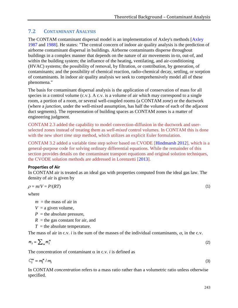
Theoretical Background – Contaminant Analysis
243
7.2 CONTAMINANT ANALYSIS
The CONTAM contaminant dispersal model is an implementation of Axley's methods [Axley
1987 and 1988]. He states: "The central concern of indoor air quality analysis is the prediction of
airborne contaminant dispersal in buildings. Airborne contaminants disperse throughout
buildings in a complex manner that depends on the nature of air movements in-to, out-of, and
within the building system; the influence of the heating, ventilating, and air-conditioning
(HVAC) systems; the possibility of removal, by filtration, or contribution, by generation, of
contaminants; and the possibility of chemical reaction, radio-chemical decay, settling, or sorption
of contaminants. In indoor air quality analysis we seek to comprehensively model all of these
phenomena."
The basis for contaminant dispersal analysis is the application of conservation of mass for all
species in a control volume (c.v.). A c.v. is a volume of air which may correspond to a single
room, a portion of a room, or several well-coupled rooms (a CONTAM zone) or the ductwork
(where a junction, under the well-mixed assumption, has half the volume of each of the adjacent
duct segments). The representation of building spaces as CONTAM zones is a matter of
engineering judgment.
CONTAM 2.3 added the capability to model convection-diffusion in the ductwork and user-
selected zones instead of treating them as well-mixed control volumes. In CONTAM this is done
with the new short time step method, which utilizes an explicit Euler formulation.
CONTAM 3.2 added a variable time step solver based on CVODE [Hindmarsh 2012], which is a
general-purpose code for solving ordinary differential equations. While the remainder of this
section provides details on the contaminant transport equations and original solution techniques,
the CVODE solution methods are addressed in Lorenzetti [2013].
Properties of Air In CONTAM air is treated as an ideal gas with properties computed from the ideal gas law. The
density of air is given by
= m/V = P/(RT) (1)
where
m = the mass of air in
V = a given volume,
P = the absolute pressure,
R = the gas constant for air, and
T = the absolute temperature.
The mass of air in c.v. i is the sum of the masses of the individual contaminants, , in the c.v.
(2)
The concentration of contaminant in c.v. i is defined as
(3)
In CONTAM concentration refers to a mass ratio rather than a volumetric ratio unless otherwise
specified.
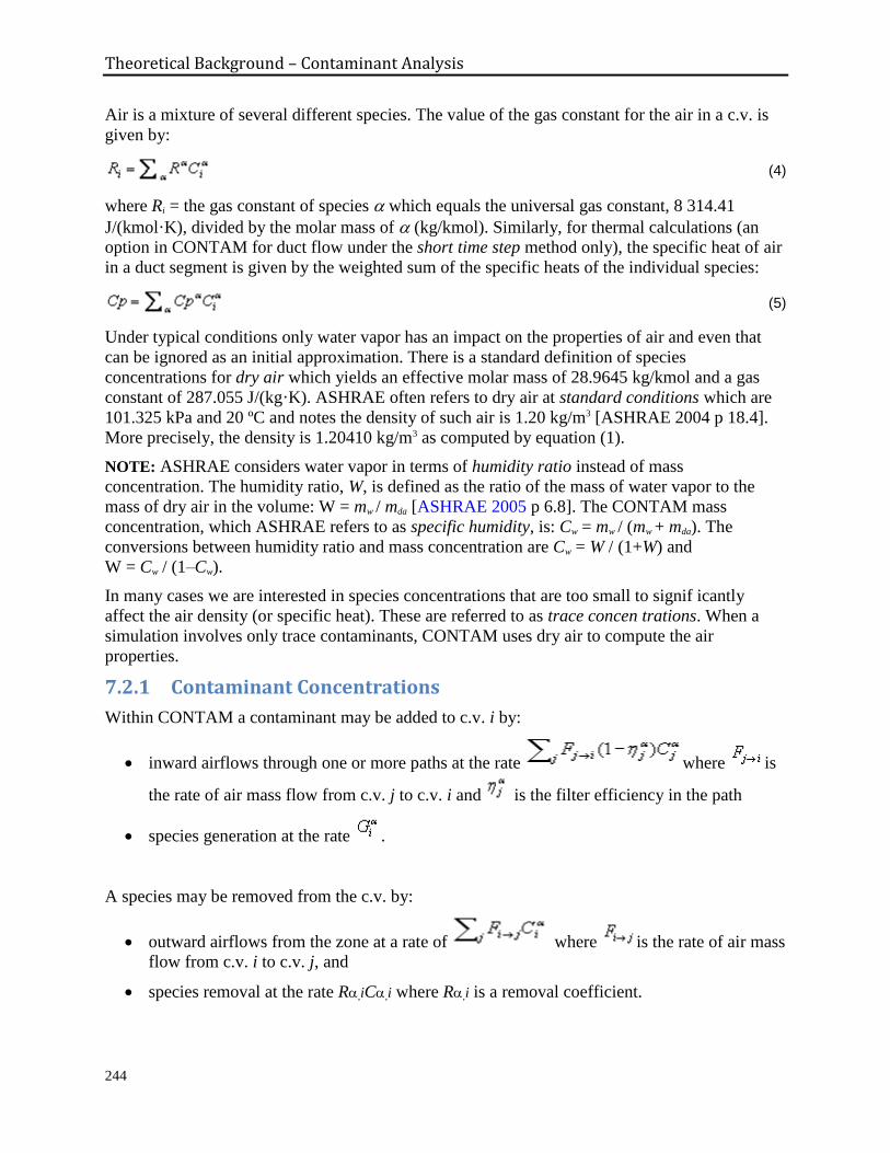
Theoretical Background – Contaminant Analysis
244
Air is a mixture of several different species. The value of the gas constant for the air in a c.v. is
given by:
(4)
where Ri = the gas constant of species which equals the universal gas constant, 8 314.41
J/(kmol·K), divided by the molar mass of (kg/kmol). Similarly, for thermal calculations (an
option in CONTAM for duct flow under the short time step method only), the specific heat of air
in a duct segment is given by the weighted sum of the specific heats of the individual species:
(5)
Under typical conditions only water vapor has an impact on the properties of air and even that
can be ignored as an initial approximation. There is a standard definition of species
concentrations for dry air which yields an effective molar mass of 28.9645 kg/kmol and a gas
constant of 287.055 J/(kg·K). ASHRAE often refers to dry air at standard conditions which are
101.325 kPa and 20 ºC and notes the density of such air is 1.20 kg/m3 [ASHRAE 2004 p 18.4].
More precisely, the density is 1.20410 kg/m3 as computed by equation (1).
NOTE: ASHRAE considers water vapor in terms of humidity ratio instead of mass
concentration. The humidity ratio, W, is defined as the ratio of the mass of water vapor to the
mass of dry air in the volume: W = mw / mda [ASHRAE 2005 p 6.8]. The CONTAM mass
concentration, which ASHRAE refers to as specific humidity, is: Cw = mw / (mw
+ mda). The
conversions between humidity ratio and mass concentration are Cw = W / (1+W) and
W = Cw / (1–Cw).
In many cases we are interested in species concentrations that are too small to signif icantly
affect the air density (or specific heat). These are referred to as trace concen trations. When a
simulation involves only trace contaminants, CONTAM uses dry air to compute the air
properties.
7.2.1 Contaminant Concentrations
Within CONTAM a contaminant may be added to c.v. i by:
inward airflows through one or more paths at the rate where is
the rate of air mass flow from c.v. j to c.v. i and is the filter efficiency in the path
species generation at the rate .
A species may be removed from the c.v. by:
outward airflows from the zone at a rate of where is the rate of air mass
flow from c.v. i to c.v. j, and
species removal at the rate R,iC,i where R,i is a removal coefficient.
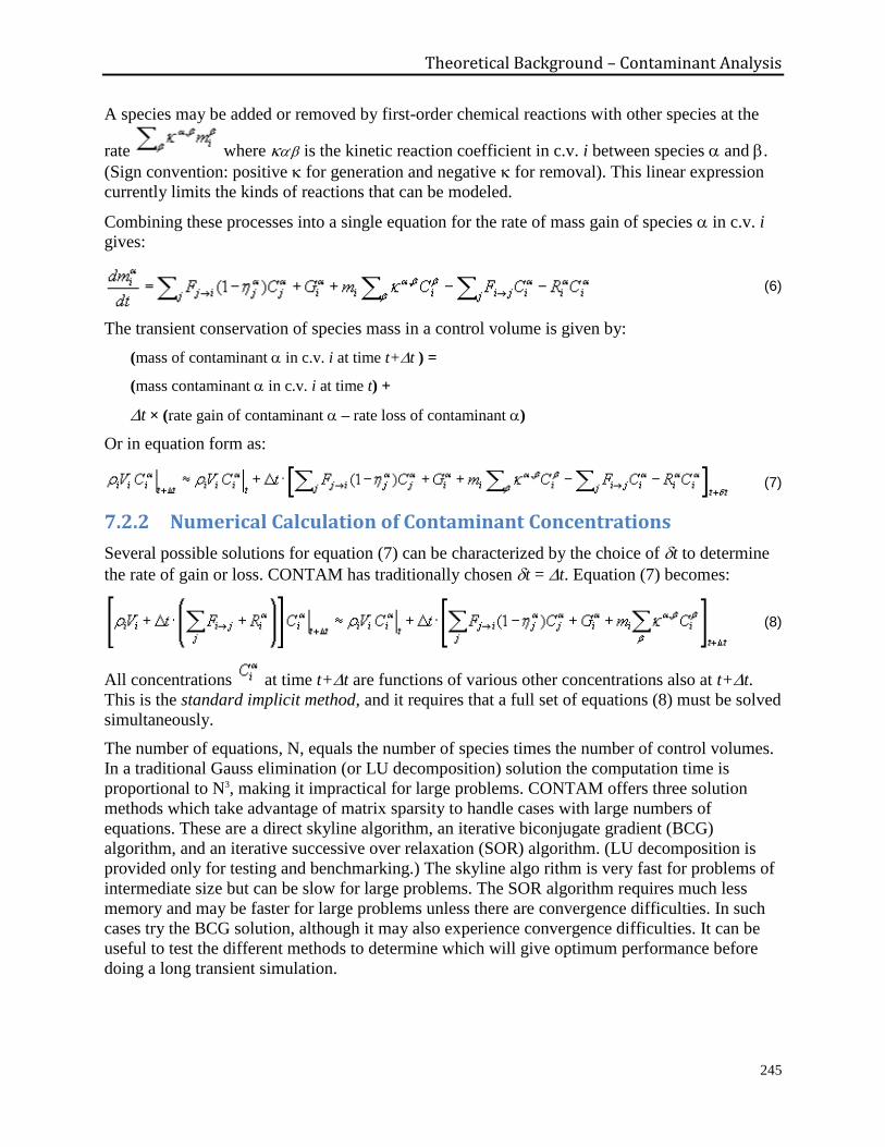
Theoretical Background – Contaminant Analysis
245
A species may be added or removed by first-order chemical reactions with other species at the
rate where , is the kinetic reaction coefficient in c.v. i between species and .
(Sign convention: positive for generation and negative for removal). This linear expression
currently limits the kinds of reactions that can be modeled.
Combining these processes into a single equation for the rate of mass gain of species in c.v. i
gives:
(6)
The transient conservation of species mass in a control volume is given by:
(mass of contaminant in c.v. i at time t+t ) =
(mass contaminant in c.v. i at time t) +
t × (rate gain of contaminant – rate loss of contaminant )
Or in equation form as:
(7)
7.2.2 Numerical Calculation of Contaminant Concentrations
Several possible solutions for equation (7) can be characterized by the choice of t to determine
the rate of gain or loss. CONTAM has traditionally chosen t = t. Equation (7) becomes:
(8)
All concentrations at time t+t are functions of various other concentrations also at t+t.
This is the standard implicit method, and it requires that a full set of equations (8) must be solved
simultaneously.
The number of equations, N, equals the number of species times the number of control volumes.
In a traditional Gauss elimination (or LU decomposition) solution the computation time is
proportional to N3, making it impractical for large problems. CONTAM offers three solution
methods which take advantage of matrix sparsity to handle cases with large numbers of
equations. These are a direct skyline algorithm, an iterative biconjugate gradient (BCG)
algorithm, and an iterative successive over relaxation (SOR) algorithm. (LU decomposition is
provided only for testing and benchmarking.) The skyline algo rithm is very fast for problems of
intermediate size but can be slow for large problems. The SOR algorithm requires much less
memory and may be faster for large problems unless there are convergence difficulties. In such
cases try the BCG solution, although it may also experience convergence difficulties. It can be
useful to test the different methods to determine which will give optimum performance before
doing a long transient simulation.
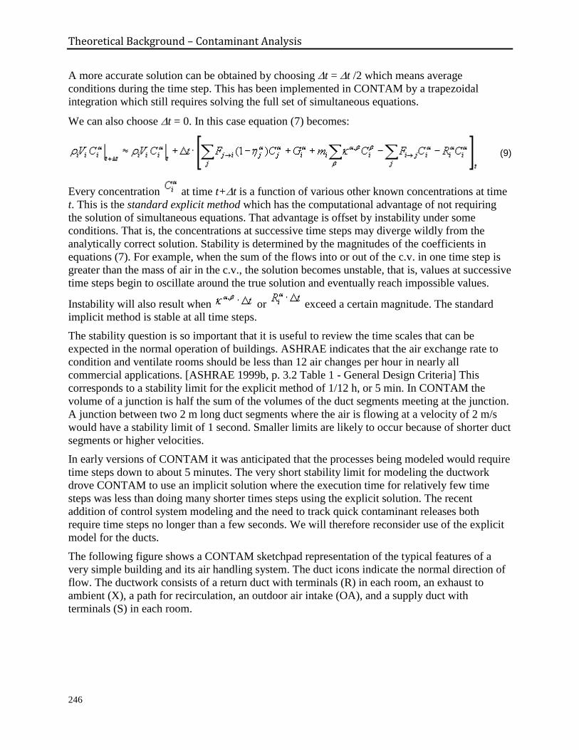
Theoretical Background – Contaminant Analysis
246
A more accurate solution can be obtained by choosing t = t /2 which means average
conditions during the time step. This has been implemented in CONTAM by a trapezoidal
integration which still requires solving the full set of simultaneous equations.
We can also choose t = 0. In this case equation (7) becomes:
(9)
Every concentration at time t+t is a function of various other known concentrations at time
t. This is the standard explicit method which has the computational advantage of not requiring
the solution of simultaneous equations. That advantage is offset by instability under some
conditions. That is, the concentrations at successive time steps may diverge wildly from the
analytically correct solution. Stability is determined by the magnitudes of the coefficients in
equations (7). For example, when the sum of the flows into or out of the c.v. in one time step is
greater than the mass of air in the c.v., the solution becomes unstable, that is, values at successive
time steps begin to oscillate around the true solution and eventually reach impossible values.
Instability will also result when or exceed a certain magnitude. The standard
implicit method is stable at all time steps.
The stability question is so important that it is useful to review the time scales that can be
expected in the normal operation of buildings. ASHRAE indicates that the air exchange rate to
condition and ventilate rooms should be less than 12 air changes per hour in nearly all
commercial applications. [ASHRAE 1999b, p. 3.2 Table 1 - General Design Criteria] This
corresponds to a stability limit for the explicit method of 1/12 h, or 5 min. In CONTAM the
volume of a junction is half the sum of the volumes of the duct segments meeting at the junction.
A junction between two 2 m long duct segments where the air is flowing at a velocity of 2 m/s
would have a stability limit of 1 second. Smaller limits are likely to occur because of shorter duct
segments or higher velocities.
In early versions of CONTAM it was anticipated that the processes being modeled would require
time steps down to about 5 minutes. The very short stability limit for modeling the ductwork
drove CONTAM to use an implicit solution where the execution time for relatively few time
steps was less than doing many shorter times steps using the explicit solution. The recent
addition of control system modeling and the need to track quick contaminant releases both
require time steps no longer than a few seconds. We will therefore reconsider use of the explicit
model for the ducts.
The following figure shows a CONTAM sketchpad representation of the typical features of a
very simple building and its air handling system. The duct icons indicate the normal direction of
flow. The ductwork consists of a return duct with terminals (R) in each room, an exhaust to
ambient (X), a path for recirculation, an outdoor air intake (OA), and a supply duct with
terminals (S) in each room.
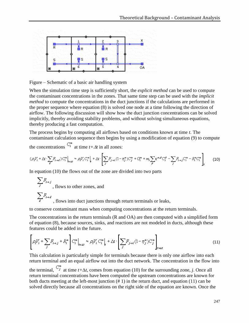
Theoretical Background – Contaminant Analysis
247
Figure – Schematic of a basic air handling system
When the simulation time step is sufficiently short, the explicit method can be used to compute
the contaminant concentrations in the zones. That same time step can be used with the implicit
method to compute the concentrations in the duct junctions if the calculations are performed in
the proper sequence where equation (8) is solved one node at a time following the direction of
airflow. The following discussion will show how the duct junction concentrations can be solved
implicitly, thereby avoiding stability problems, and without solving simultaneous equations,
thereby producing a fast computation.
The process begins by computing all airflows based on conditions known at time t. The
contaminant calculation sequence then begins by using a modification of equation (9) to compute
the concentrations at time t+t in all zones:
(10)
In equation (10) the flows out of the zone are divided into two parts
, flows to other zones, and
, flows into duct junctions through return terminals or leaks,
to conserve contaminant mass when computing concentrations at the return terminals.
The concentrations in the return terminals (R and OA) are then computed with a simplified form
of equation (8), because sources, sinks, and reactions are not modeled in ducts, although these
features could be added in the future.
(11)
This calculation is particularly simple for terminals because there is only one airflow into each
return terminal and an equal airflow out into the duct network. The concentration in the flow into
the terminal, at time t+t, comes from equation (10) for the surrounding zone, j. Once all
return terminal concentrations have been computed the upstream concentrations are known for
both ducts meeting at the left-most junction (# 1) in the return duct, and equation (11) can be
solved directly because all concentrations on the right side of the equation are known. Once the
Theoretical Background – Contaminant Analysis
248
junction #1 concentrations have been computed all upstream concentrations are known for the
next junction to the right (# 2) along the return duct and its concentrations can then be computed.
This process continues around the ductwork until the concentrations at all junctions and all
supply terminals have been computed. This implicit calculation of the concentrations in the duct
junctions is unconditionally stable, so overall stability is determined by conditions in the zones.
CONTAM 2.4 adds this process calling it the short time step method (STS).
Reactions may include coefficients that lead to instabilities for an explicit simulation. Very fast
reactions would produce such coefficients. Therefore, the STS method processes reactions by an
implicit calculation involving only the contaminants in the c.v. after all other calculations have
been performed for the time step.
7.2.3 One-Dimensional Convection-Diffusion Flow
Although it is possible to use a time step as short as one second in CONTAM, this may not
produce a more accurate simulation of transient concentrations because of the use of control
volumes which are treated as well-mixed. For example, consider the sudden release of a
contaminant at one end of a 10 m long zone with air flowing at a typical 0.2 m/s from the release
point toward a doorway at the other end. It would take about 50 seconds for the contaminant to
reach that doorway and begin entering the next zone. In the well-mixed zone model the sudden
release will instantly produce a uniform concentration (equal to the mass released divided by the
mass of air) everywhere in the zone, even at the far end 10 m from the source, and begins
entering the adjacent zone within one time step.
The well-mixed zone model is appropriate when the time step is longer than the mixing time of
the zone. Conventional HVAC systems attempt to produce well mixed zones, but the mixing
time is on the order of a few minutes rather than seconds.
The standard numerical solution to this problem is to create smaller control volumes whose size
is similar to the distance traveled in one time step. This is done in the computational fluid
dynamics (CFD) models that consider mass, momentum, and energy in computing the flow field
in a space that has been divided into many control volumes. Conventional CFD might divide a
volume into 30 cells along each of the three directions. This increases the computation effort
from one large "cell" per zone to 27,000 (=30×30×30) cells per zone. This analysis approach is
not practical for a building containing many zones.
One-dimensional convection-diffusion flow has been introduced to CONTAM as a compromise
between simple, and fast, well-mixed zones and a full CFD simulation. CONTAM 2.4 includes
the option of modeling detailed contaminant migration in one, user-defined direction through a
zone and or an entire duct system. This one-dimensional model is obviously appropriate for flow
through a duct and reasonably appropriate for a long hallway or a zone using a displacement
ventilation system. Its use in more conventional well-mixed zones is problematic because of the
presence of supply air jets and areas of recirculation.
Contaminant flow in one direction consists of a mixture of convection, the bulk movement of air,
and diffusion, the mixing of the contaminant within the air. CONTAM’s primary 1-D convection
diffusion model is taken directly from the finite volume method developed by Patankar [Patankar
1980] and described in more detail by Versteeg and Malalasekera [Versteeg and Malalasekera
1995]. This model divides the zone into a number of equal-length cells and uses an implicit
method (with a fast tri-diagonal equation solver) to guarantee stability in computing the
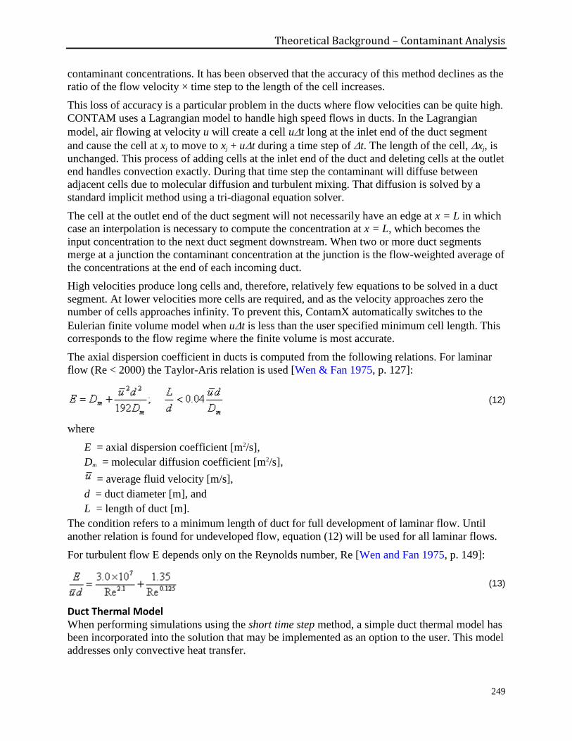
Theoretical Background – Contaminant Analysis
249
contaminant concentrations. It has been observed that the accuracy of this method declines as the
ratio of the flow velocity × time step to the length of the cell increases.
This loss of accuracy is a particular problem in the ducts where flow velocities can be quite high.
CONTAM uses a Lagrangian model to handle high speed flows in ducts. In the Lagrangian
model, air flowing at velocity u will create a cell ut long at the inlet end of the duct segment
and cause the cell at xj to move to xj + ut during a time step of t. The length of the cell, xj, is
unchanged. This process of adding cells at the inlet end of the duct and deleting cells at the outlet
end handles convection exactly. During that time step the contaminant will diffuse between
adjacent cells due to molecular diffusion and turbulent mixing. That diffusion is solved by a
standard implicit method using a tri-diagonal equation solver.
The cell at the outlet end of the duct segment will not necessarily have an edge at x = L in which
case an interpolation is necessary to compute the concentration at x = L, which becomes the
input concentration to the next duct segment downstream. When two or more duct segments
merge at a junction the contaminant concentration at the junction is the flow-weighted average of
the concentrations at the end of each incoming duct.
High velocities produce long cells and, therefore, relatively few equations to be solved in a duct
segment. At lower velocities more cells are required, and as the velocity approaches zero the
number of cells approaches infinity. To prevent this, ContamX automatically switches to the
Eulerian finite volume model when ut is less than the user specified minimum cell length. This
corresponds to the flow regime where the finite volume is most accurate.
The axial dispersion coefficient in ducts is computed from the following relations. For laminar
flow (Re < 2000) the Taylor-Aris relation is used [Wen & Fan 1975, p. 127]:
(12)
where
E = axial dispersion coefficient [m2/s],
Dm = molecular diffusion coefficient [m2/s],
= average fluid velocity [m/s],
d = duct diameter [m], and
L = length of duct [m].
The condition refers to a minimum length of duct for full development of laminar flow. Until
another relation is found for undeveloped flow, equation (12) will be used for all laminar flows.
For turbulent flow E depends only on the Reynolds number, Re [Wen and Fan 1975, p. 149]:
(13)
Duct Thermal Model When performing simulations using the short time step method, a simple duct thermal model has
been incorporated into the solution that may be implemented as an option to the user. This model
addresses only convective heat transfer.

Theoretical Background – Contaminant Analysis
250
Conservation of thermal energy is analogous to the conservation of contaminant mass in a
control volume:
(energy at time t+t ) = (energy at time t) + t •(rate of energy gain – rate of energy loss)
Replace the concentration terms, , in equation (8) with specific energy, CpiTi:
(14)
where
Cpi = specific heat of c.v. i, and
Ti = temperature of c.v. i.
This is done only for ducts because the energy in the moving air dominants the solution in a well
designed and well built duct system. That is not the case for zones where conductive and airflow
heat transfers are of a similar scale. This model ignores heat exchange with the ductwork and its
transient impact. However, the model should still be a useful help in computing the draft of a
chimney.
7.2.4 Contaminant Source/Sink Elements
CONTAM allows you to define the generation, G, and removal, R, coefficients for some
simple cases.
Constant Coefficient Model The constant coefficient or general source/sink model uses the following equation:
(15)
where S is called the contaminant "source strength". The CONTAM internal units for the
terms in equation (16) are: C [kg / kgair], G, S [kg / s], and R [kgair / s]. You may express
these values in a large number of units with automatic conversion to the internal values.
For a room air filtering device, G = 0.0 and R = f•e where f is the flow rate of the room air
passing through the filter and e is the single pass removal efficiency of the device.
Pressure Driven Model The pressure driven source/sink model is intended to model contaminant sources which are
governed by the inside-outside pressure difference, such as radon or soil gas entry into a
basement. In this case the source equation is:
(16)
Cutoff Concentration Model For volatile organic compounds the source equation is sometimes expressed in the form
(17)
where Ccutoff is the cutoff concentration at which emission ceases.
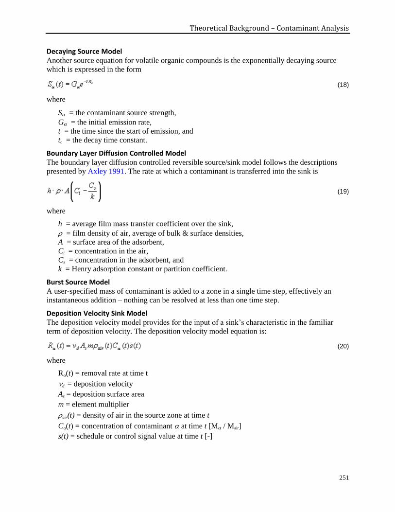
Theoretical Background – Contaminant Analysis
251
Decaying Source Model Another source equation for volatile organic compounds is the exponentially decaying source
which is expressed in the form
(18)
where
S = the contaminant source strength,
G = the initial emission rate,
t = the time since the start of emission, and
tc = the decay time constant.
Boundary Layer Diffusion Controlled Model The boundary layer diffusion controlled reversible source/sink model follows the descriptions
presented by Axley 1991. The rate at which a contaminant is transferred into the sink is
(19)
where
h = average film mass transfer coefficient over the sink,
= film density of air, average of bulk & surface densities,
A = surface area of the adsorbent,
Ci = concentration in the air,
Cs = concentration in the adsorbent, and
k = Henry adsorption constant or partition coefficient.
Burst Source Model A user-specified mass of contaminant is added to a zone in a single time step, effectively an
instantaneous addition – nothing can be resolved at less than one time step.
Deposition Velocity Sink Model The deposition velocity model provides for the input of a sink’s characteristic in the familiar
term of deposition velocity. The deposition velocity model equation is:
(20)
where
R(t) = removal rate at time t
d = deposition velocity
As = deposition surface area
m = element multiplier
air(t) = density of air in the source zone at time t
C(t) = concentration of contaminant at time t [M / Mair]
s(t) = schedule or control signal value at time t [-]
Theoretical Background – Contaminant Analysis
252
Deposition Rate Sink Model The deposition rate model provides for the input of a sink’s characteristic in the familiar term of
deposition or removal rate. The deposition rate model equation is:
(21)
where
kd = Deposition rate [1/T]
Vz = Zone volume [M3]
other terms are the same as for the Deposition Velocity Sink Model.
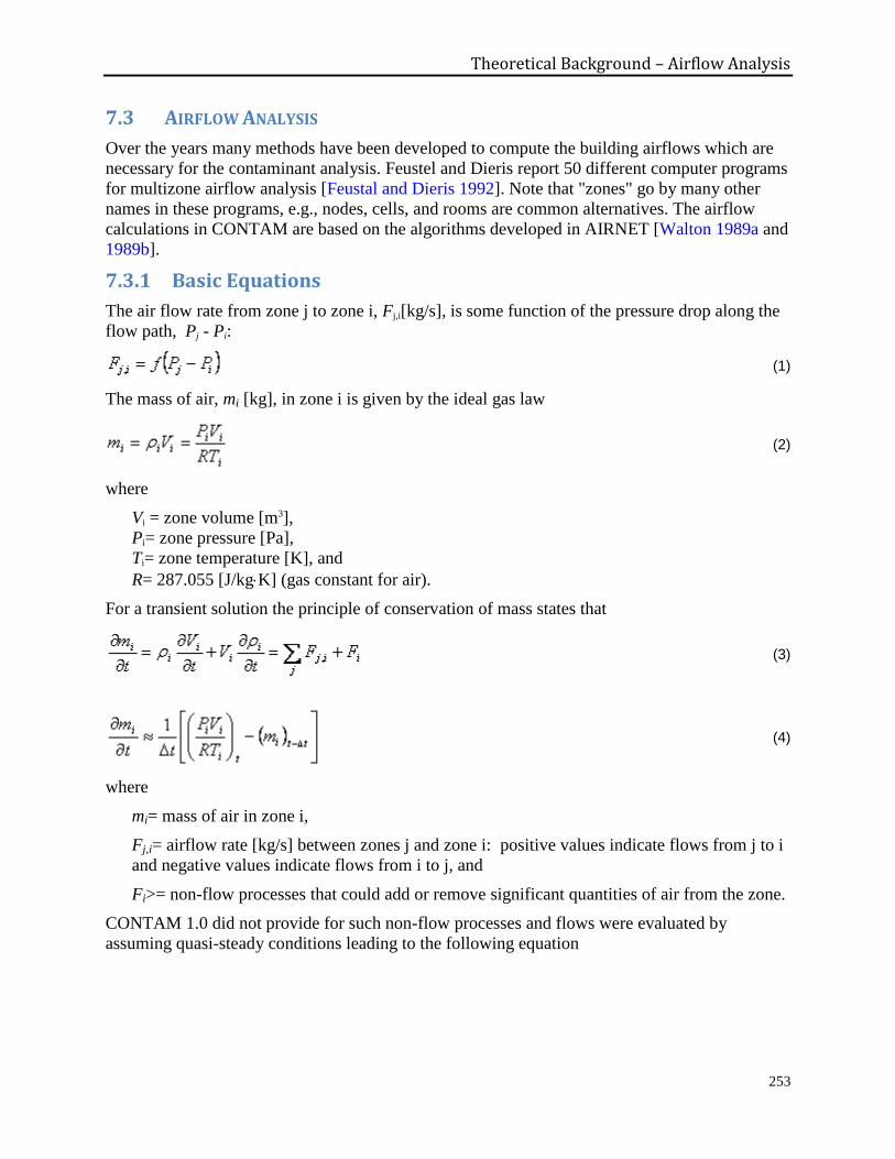
Theoretical Background – Airflow Analysis
253
7.3 AIRFLOW ANALYSIS
Over the years many methods have been developed to compute the building airflows which are
necessary for the contaminant analysis. Feustel and Dieris report 50 different computer programs
for multizone airflow analysis [Feustal and Dieris 1992]. Note that "zones" go by many other
names in these programs, e.g., nodes, cells, and rooms are common alternatives. The airflow
calculations in CONTAM are based on the algorithms developed in AIRNET [Walton 1989a and
1989b].
7.3.1 Basic Equations
The air flow rate from zone j to zone i, Fj,i[kg/s], is some function of the pressure drop along the
flow path, Pj - Pi:
(1)
The mass of air, mi [kg], in zone i is given by the ideal gas law
(2)
where
Vi = zone volume [m3],
Pi= zone pressure [Pa],
Ti= zone temperature [K], and
R= 287.055 [J/kgK] (gas constant for air).
For a transient solution the principle of conservation of mass states that
(3)
(4)
where
mi= mass of air in zone i,
Fj,i= airflow rate [kg/s] between zones j and zone i: positive values indicate flows from j to i
and negative values indicate flows from i to j, and
Fi>= non-flow processes that could add or remove significant quantities of air from the zone.
CONTAM 1.0 did not provide for such non-flow processes and flows were evaluated by
assuming quasi-steady conditions leading to the following equation
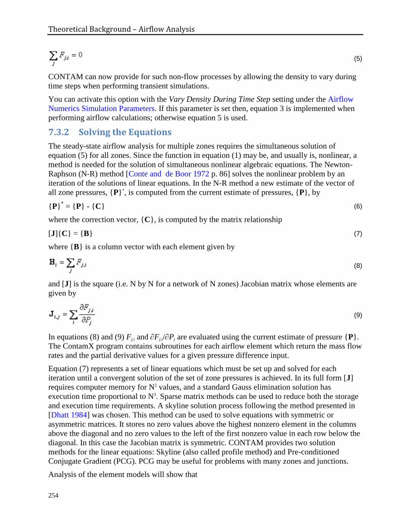
Theoretical Background – Airflow Analysis
254
(5)
CONTAM can now provide for such non-flow processes by allowing the density to vary during
time steps when performing transient simulations.
You can activate this option with the Vary Density During Time Step setting under the Airflow
Numerics Simulation Parameters. If this parameter is set then, equation 3 is implemented when
performing airflow calculations; otherwise equation 5 is used.
7.3.2 Solving the Equations
The steady-state airflow analysis for multiple zones requires the simultaneous solution of
equation (5) for all zones. Since the function in equation (1) may be, and usually is, nonlinear, a
method is needed for the solution of simultaneous nonlinear algebraic equations. The Newton-
Raphson (N-R) method [Conte and de Boor 1972 p. 86] solves the nonlinear problem by an
iteration of the solutions of linear equations. In the N-R method a new estimate of the vector of
all zone pressures, {P}*, is computed from the current estimate of pressures, {P}, by
{P}* = {P} - {C} (6)
where the correction vector, {C}, is computed by the matrix relationship
[J]{C} = {B} (7)
where {B} is a column vector with each element given by
(8)
and [J] is the square (i.e. N by N for a network of N zones) Jacobian matrix whose elements are
given by
(9)
In equations (8) and (9) Fj,i and Fj,i/Pj are evaluated using the current estimate of pressure {P}.
The ContamX program contains subroutines for each airflow element which return the mass flow
rates and the partial derivative values for a given pressure difference input.
Equation (7) represents a set of linear equations which must be set up and solved for each
iteration until a convergent solution of the set of zone pressures is achieved. In its full form [J]
requires computer memory for N2 values, and a standard Gauss elimination solution has
execution time proportional to N3. Sparse matrix methods can be used to reduce both the storage
and execution time requirements. A skyline solution process following the method presented in
[Dhatt 1984] was chosen. This method can be used to solve equations with symmetric or
asymmetric matrices. It stores no zero values above the highest nonzero element in the columns
above the diagonal and no zero values to the left of the first nonzero value in each row below the
diagonal. In this case the Jacobian matrix is symmetric. CONTAM provides two solution
methods for the linear equations: Skyline (also called profile method) and Pre-conditioned
Conjugate Gradient (PCG). PCG may be useful for problems with many zones and junctions.
Analysis of the element models will show that
Theoretical Background – Airflow Analysis
255
(10)
This condition allows a solution without pivoting, although scaling may be useful. Note that the
degree of sparsity of the Jacobian matrix after factoring is dependent on the ordering of the
zones. Ordering can be improved by various algorithms or rules-of-thumb. In AIRNET it was
easy to define an airflow network which had no unique solution. The ContamW user interface
insures the correct interconnection of the airflow elements in the network.
CONTAM allows zones with either known or unknown pressures. The constant pressure zones
are included in the system of equations and equation (7) is processed so as to not change those
zone pressures. This gives flexibility in defining the airflow network while maintaining the
symmetric set of equations. A sufficient condition for the Jacobian to be nonsingular [Axley
1987] is that all of the unknown pressure zones be linked by pressure dependent flow paths to (a)
constant pressure zone(s). In CONTAM the ambient (or outdoor) air is treated as a constant
pressure zone. The ambient zone pressure is assumed to be zero for the flow calculation causing
the computed zone pressures to be values relative to the true ambient pressure and helping to
maintain numerical significance in calculating P.
Conservation of mass at each zone provides the convergence criterion for the N-R iterations.
That is, when equation (4) is satisfied for all zones for the current system pressure estimate, the
solution has converged. Sufficient accuracy is attained by testing for relative convergence at each
zone:
(11)
with a test (Fj,i < 1, the absolute convergence factor) to prevent division by zero. The
magnitude of can be established by considering the use of the calculated airflows, such as in an
energy balance. In any case, round-off errors may prevent perfect convergence ( = 0).
Numerical tests of the N-R method solution indicated occasional instances of very slow
convergence as the iterations almost oscillate between two different sets of values. In AIRNET,
this was handled by a Steffensen acceleration process. More recent tests by the author and by
Wray [Wray 1993] indicate that the use of a simpler constant under-relaxation coefficient
produces a faster, reliable convergence acceleration process. Equation (6) for the iteration
process becomes
{P}* = {P} - {C} (12)
where is the relaxation coefficient. A relaxation coefficient of 0.75 has been found to be usable
for a broad range of airflow networks. This value is not a true optimum but appears to work quite
well without the computational cost of finding the theoretically optimum value.
When convergence is progressing rapidly, under-relaxation ( < 1) slows convergence compared
to no relaxation. To prevent this a global convergence value is computed:
Theoretical Background – Airflow Analysis
256
(13)
When * < , is set to 1. Currently CONTAM uses = 30%. This often reduces the number
of iterations. This is simple under-relaxation. CONTAM also may alternatively use a simple trust
region method implemented by David M. Lorenzetti based on [Dennis and Schnabel 1996].
Newton's method requires an initial set of values for the zone pressures. These may be obtained
by including in each airflow element model a linear approximation relating the flow to the
pressure drop:
(14)
Conservation of mass at each zone leads to a set of linear equations of the form
[A]{P} = {B} (15)
Matrix [A] in equation (15) has the same sparsity pattern as [J] in equation (7) allowing use of
the same sparse matrix solution process for both equations. This initialization handles stack
effects very well and tends to establish the proper directions for the flows. The linear
approximation is conveniently provided by the laminar regime of the element models used by
CONTAM. When solving a set of similar problems, as when approximating a transient solution
by successive steady-state solutions, it tends to be preferable to use the previous solution for the
zone pressures as the initial values for the new problem.
7.3.3 Airflow Elements
Infiltration is the result of air flowing through openings, large and small, intentional and
accidental, in the building envelope. Simulation programs require a mathematical model of the
flow characteristics of the openings. For a general introduction see Chapter 27 of [ASHRAE
2005] and section 2.2 of [Feustel 1990].
Flow within each airflow element is assumed to be governed by Bernoulli's equation:
(16)
where
P= total pressure drop between points 1 and 2
P1, P2= entry and exit static pressures
V1, V2= entry and exit velocities
= air density
g= acceleration of gravity (9.81 m/s2)
z1, z2= entry and exit elevations.
The following parameters apply to the zones: pressure, temperature (to compute density and
viscosity), and elevation. The zone elevation values are used to determine stack effect pressures.
When the zone represents a room, the airflow elements may connect with the room at other than
its reference elevation. The hydrostatic equation is used to relate the pressure difference across a

Theoretical Background – Airflow Analysis
257
flow element to the elevations of the element ends and the zone elevations, assuming the air in
the room is at constant temperature. Pressure terms can be rearranged and a possible wind
pressure for building envelope openings added to give
(17)
where
Pi, Pj= total pressures at zones i and j
PS= pressure difference due to density and elevation differences, and
PW= pressure difference due to wind.
Equation (17) establishes a sign convention for direction of flow: positive is from zone j to zone
i. Since the airflow elements will be described by a relationship of the form w = f(P), the partial
derivatives needed for [J] in equation (9) are related by w/Pj = -w/Pi which establishes the
relation in equation (10). Many forms of airflow elements are available in CONTAM.
Powerlaw Flow Elements
Most infiltration models are based on the following empirical (powerlaw) relationship between
the flow and the pressure difference across a crack or opening in the building envelope:
(18)
The volumetric flow rate, Q [m3/s], is a simple function of the pressure drop, P [Pa], across the
opening. A common variation of the powerlaw equation is:
(19)
where the mass flow rate, F [kg/s], is a simple function of the pressure drop. A third variation is
related to the orifice equation:
(20)
where
Cd= discharge coefficient, and
A= orifice opening area.
Theoretically, the value of the flow exponent should lie between 0.5 and 1.0. Large openings are
characterized by values very close to 0.5, while values near 0.65 have been found for small
crack-like openings.
The primary advantage of equations (18-20) for describing airflow components is the simple
calculation of the partial derivatives for the Newton's method solution of the simultaneous
equations:
and
(21)
The sign in equations (21) will agree with the sign of F. However, there is also a problem with
equations (21): the derivatives become unbounded as the pressure drop (and the flow) go to zero.
Theoretical Background – Airflow Analysis
258
A simple way to avoid this problem is suggested by what physically happens at low flow rates:
the physical character of the flow (and the form of the equation) changes. It goes from turbulent
to laminar. Equations (18-20) can be replaced by
(22)
where
Ck= laminar flow coefficient, and
= viscosity.
The partial derivatives are simple constants:
and
(23)
The origin of this laminar relationship is shown by the duct equations in the next section. This
technique has been independently discovered and used by several researchers [Axley 1987] and
[Isaacs 1980]. Although there is physical reason for using equation (22) at low pressure drops, its
purpose here is to assure convergence of the equations when P approaches zero for one of the
many flow paths in a complex network, instead of accurately representing airflows which are too
small to be of interest. Because the linear flow expression is not used as a true flow model but as
a mathematical artifice, it is not necessary to adjust its flow coefficient. Given the uncertainty in
estimating the temperature of the air as it flows through an opening, especially a crack, this
additional detail is of debatable usefulness.
The CONTAM functions for powerlaw elements calculate flows using both the laminar and the
turbulent models and select the method giving the smaller magnitude flow. There is a
discontinuity in the derivative of the F(P) curve where the two equations intersect. This
discontinuity is a violation of one of the sufficient conditions for convergence of Newton's
method [Conte and de Boor 1972, p. 86]. However, numerical tests conducted by the author for
flows at that point using a small airflow network have shown no convergence problem.
Temperature Dependence
It is useful to think of the coefficient C as a simple constant, C, evaluated at a particular set of
conditions (0, 0 and 0=0/0) multiplied by a correction factor to account for actual air
properties. Equations (18-20) are converted to a common form and summarized below with their
appropriate temperature correction factors.
Correction Factor
(24)
CONTAM uses the following formulae for computing and :
= P / (287.055 T)
Theoretical Background – Airflow Analysis
259
= 3.714310-6 + 4.928610-8T
= /
Using reference conditions of standard atmospheric pressure and 20C gives o = 1.2041 kg/m3
and o = 1.508310-5 m2/s.
Fitting Powerlaw Coefficients
Experimental data can be used to determine the coefficients in the orifice form of the powerlaw
equation:
(25)
If n is known or can be assumed, Cb, in equation (24), can be computed from the inverse of
equation (25)
(26)
When two points (F1, P1) and (F2, P2), are known, n can be computed from:
(27)
with Cb then computed from equation (26).
Leakage Areas
The powerlaw model can be used with the component leakage area formulation which has been
used to characterize openings for infiltration calculations [ASHRAE 2001, p. 25.18]. The
leakage area is based on a series of pressurization tests where the airflow rate is measured at a
series of pressure differences ranging from about 10 Pa to 75 Pa. The effective leakage area is
based on a rearrangement of equation (20)
(28)
where
L= equivalent or effective leakage area [m2],
Pr= reference pressure difference [Pa],
Qr= predicted airflow rate at Pr (from curve fit to pressurization test data) [m3/s], and
Cd= discharge coefficient.
There are two common sets of reference conditions:
Cd = 1.0 and Pr = 4 Pa
or
Cd = 0.6 and Pr = 10 Pa.
A leakage area can be converted to the flow coefficient by
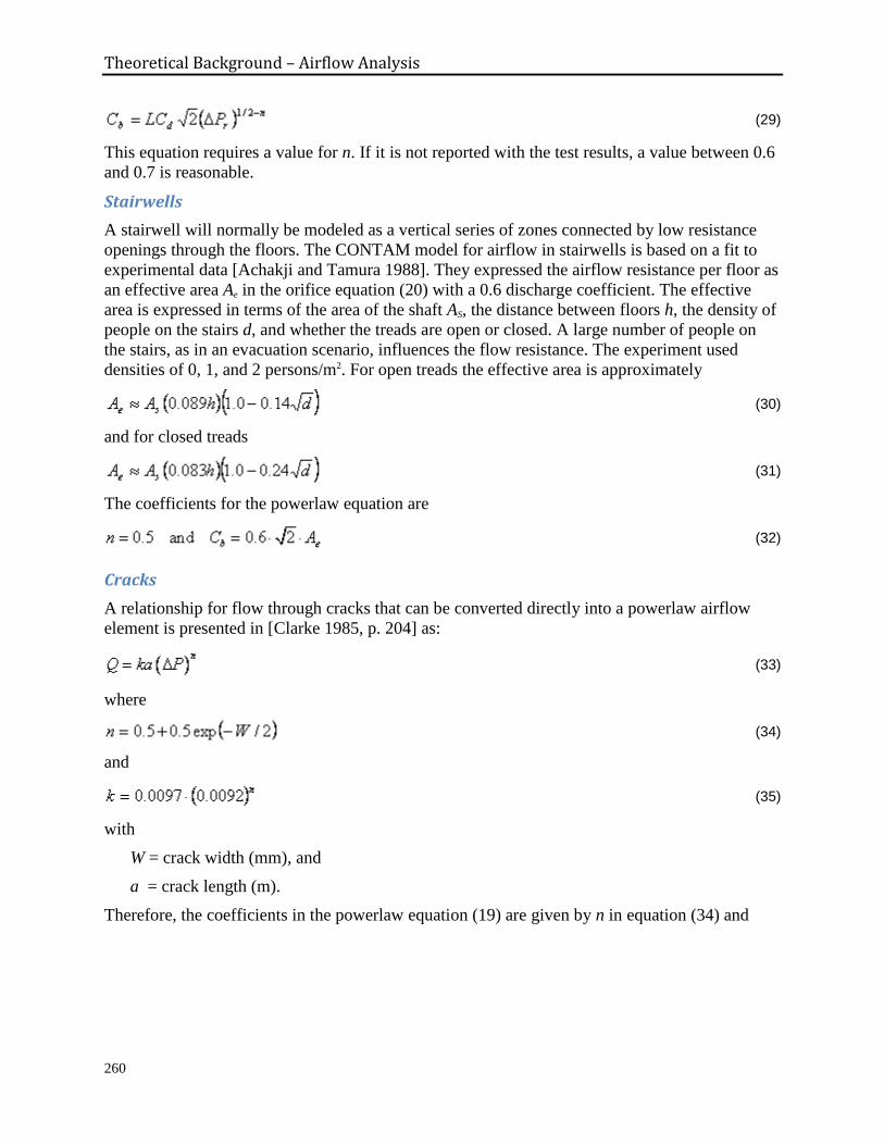
Theoretical Background – Airflow Analysis
260
(29)
This equation requires a value for n. If it is not reported with the test results, a value between 0.6
and 0.7 is reasonable.
Stairwells
A stairwell will normally be modeled as a vertical series of zones connected by low resistance
openings through the floors. The CONTAM model for airflow in stairwells is based on a fit to
experimental data [Achakji and Tamura 1988]. They expressed the airflow resistance per floor as
an effective area Ae in the orifice equation (20) with a 0.6 discharge coefficient. The effective
area is expressed in terms of the area of the shaft AS, the distance between floors h, the density of
people on the stairs d, and whether the treads are open or closed. A large number of people on
the stairs, as in an evacuation scenario, influences the flow resistance. The experiment used
densities of 0, 1, and 2 persons/m2. For open treads the effective area is approximately
(30)
and for closed treads
(31)
The coefficients for the powerlaw equation are
(32)
Cracks
A relationship for flow through cracks that can be converted directly into a powerlaw airflow
element is presented in [Clarke 1985, p. 204] as:
(33)
where
(34)
and
(35)
with
W = crack width (mm), and
a = crack length (m).
Therefore, the coefficients in the powerlaw equation (19) are given by n in equation (34) and
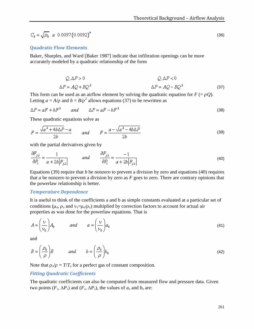
Theoretical Background – Airflow Analysis
261
(36)
Quadratic Flow Elements
Baker, Sharples, and Ward [Baker 1987] indicate that infiltration openings can be more
accurately modeled by a quadratic relationship of the form
(37)
This form can be used as an airflow element by solving the quadratic equation for F (= Q).
Letting a = A/ and b = B/2 allows equations (37) to be rewritten as
(38)
These quadratic equations solve as
(39)
with the partial derivatives given by
(40)
Equations (39) require that b be nonzero to prevent a division by zero and equations (40) requires
that a be nonzero to prevent a division by zero as F goes to zero. There are contrary opinions that
the powerlaw relationship is better.
Temperature Dependence
It is useful to think of the coefficients a and b as simple constants evaluated at a particular set of
conditions (0, 0 and 0=0/0) multiplied by correction factors to account for actual air
properties as was done for the powerlaw equations. That is
(41)
and
(42)
Note that 0/ = T/T0 for a perfect gas of constant composition.
Fitting Quadratic Coefficients
The quadratic coefficients can also be computed from measured flow and pressure data. Given
two points (F1, P1) and (F2, P2), the values of a0 and b0 are:
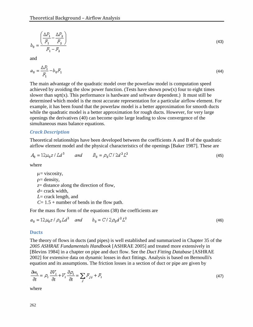
Theoretical Background – Airflow Analysis
262
(43)
and
(44)
The main advantage of the quadratic model over the powerlaw model is computation speed
achieved by avoiding the slow power function. (Tests have shown pow(x) four to eight times
slower than sqrt(x). This performance is hardware and software dependent.) It must still be
determined which model is the most accurate representation for a particular airflow element. For
example, it has been found that the powerlaw model is a better approximation for smooth ducts
while the quadratic model is a better approximation for rough ducts. However, for very large
openings the derivatives (40) can become quite large leading to slow convergence of the
simultaneous mass balance equations.
Crack Description
Theoretical relationships have been developed between the coefficients A and B of the quadratic
airflow element model and the physical characteristics of the openings [Baker 1987]. These are
(45)
where
= viscosity,
= density,
z= distance along the direction of flow,
d= crack width,
L= crack length, and
C= 1.5 + number of bends in the flow path.
For the mass flow form of the equations (38) the coefficients are
(46)
Ducts
The theory of flows in ducts (and pipes) is well established and summarized in Chapter 35 of the
2005 ASHRAE Fundamentals Handbook [ASHRAE 2005] and treated more extensively in
[Blevins 1984] in a chapter on pipe and duct flow. See the Duct Fitting Database [ASHRAE
2002] for extensive data on dynamic losses in duct fittings. Analysis is based on Bernoulli's
equation and its assumptions. The friction losses in a section of duct or pipe are given by
(47)
where
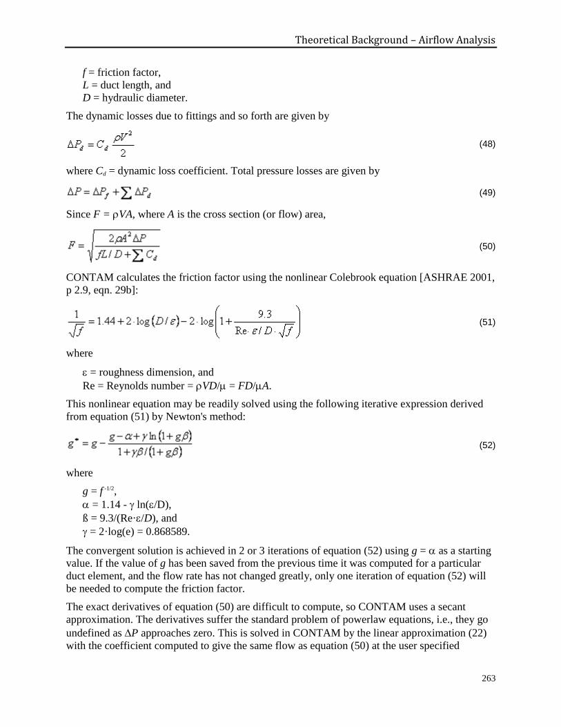
Theoretical Background – Airflow Analysis
263
f = friction factor,
L = duct length, and
D = hydraulic diameter.
The dynamic losses due to fittings and so forth are given by
(48)
where Cd = dynamic loss coefficient. Total pressure losses are given by
(49)
Since F = VA, where A is the cross section (or flow) area,
(50)
CONTAM calculates the friction factor using the nonlinear Colebrook equation [ASHRAE 2001,
p 2.9, eqn. 29b]:
(51)
where
= roughness dimension, and
Re = Reynolds number = VD/ = FD/A.
This nonlinear equation may be readily solved using the following iterative expression derived
from equation (51) by Newton's method:
(52)
where
g = f -1/2,
= 1.14 - ln(/D),
ß = 9.3/(Re·/D), and
= 2·log(e) = 0.868589.
The convergent solution is achieved in 2 or 3 iterations of equation (52) using g = as a starting
value. If the value of g has been saved from the previous time it was computed for a particular
duct element, and the flow rate has not changed greatly, only one iteration of equation (52) will
be needed to compute the friction factor.
The exact derivatives of equation (50) are difficult to compute, so CONTAM uses a secant
approximation. The derivatives suffer the standard problem of powerlaw equations, i.e., they go
undefined as P approaches zero. This is solved in CONTAM by the linear approximation (22)
with the coefficient computed to give the same flow as equation (50) at the user specified
Theoretical Background – Airflow Analysis
264
transition Reynolds number (default = 2000). A more detailed description of the flow in the
laminar region could be developed, but that would probably exceed the level of detail with which
the rest of the problem is described in CONTAM.
Terminal Loss Calculation In CONTAM, duct terminals are essentially zero-length ducts characterized by an equivalent loss
coefficient that is determined during simulation from the properties of the terminal, Ct and Cb,
and the schedule or control signal (S) acting upon the terminal.
Ce = Ct + Cb + (1-S)/S
where
Ct = terminal loss coefficient
Cb= terminal balance coefficient
Sc = schedule or control signal acting upon the terminal
S = max(1x10⁻⁶, Sc1)
Sc1= min(1, Sc)
Using this technique, an input signal Sc of 0.0 will effect a very high loss coefficient, that of 1.0
will simply provide the loss determined by the combination of Ct and Cb, Scbetween 1x10⁻⁶ and 1
will be used to increase the value of (Ct + Cb) according to the equation above, and Sc less than
0.0 will equate to 1.0, i.e., the loss can not be reduced below (Ct + Cb). The value Ce will then be
used as the dynamic loss coefficient in the duct flow equations presented above.
Fans
This section describes the theory of how forced flow elements are modeled with CONTAM.
Forced flow elements include constant flow fans and variable flow fans. Constant flow fans
include both constant volume and constant mass flow. Variable flow fans are modeled based on
the input of a fan performance curve that relates pressure drop to airflow through the fan flow
element.
Constant Flow Fans
One particularly simple but useful airflow element sets a constant flow between two nodes. Since
the flow is constant, the partial derivatives of flow with respect to the node pressures must be
zero. The constant flow element does not contribute to the Jacobian, [A], but it does add to the
right side vector, {B}.
Constant flow elements do not mathematically link the pressures of the adjacent nodes. It is
necessary that all node in the network be linked to constant pressure nodes in order to have a
unique solution. Violation of this restriction will produce a division by zero somewhere in the
solution of the equations. Consider the following simple network:
|----C1----|----F1----|----C2----|----F2----|----C3----|
P1 P2 P3 P4 P5 P6
where P1 and P6 are known pressures, and F1 and F2 are known flows. Since the flow through C2
is determined by P3 - P4, and no other flow is related to those pressures, there are not enough
Theoretical Background – Airflow Analysis
265
equations to determine P3and P4 uniquely. This is a mathematical expression of the fact that it is
possible for F1 and F2 to be assigned different flows, which produces a physically impossible
condition.
CONTAM provides two constant flow elements: one for constant mass flow and one for
constant volumetric flow.
Variable Flow Fans
The theory of flows induced by fans is summarized in Chapter 18 of the 2000 ASHRAE HVAC
Systems and Equipment Handbook [ASHRAE 2004]. More extensive treatment is given in
[Osborne 1977]. Fan performance is normally characterized by a performance curve which
relates the total pressure rise to the flow rate for a given fan speed and air density. Conversion to
another fan speed or density is done with the fan laws.
(53)
or
(54)
and
(55)
where
Q = volume flow rate,
F = mass flow rate,
P = total pressure rise,
= density,
N = rotational speed, and
subscript 0 indicates values at the rating conditions for the fan.
These laws are valid if all flow conditions at the two speeds are similar. In particular, they will
not apply at very low flows where fully turbulent conditions have not been developed.
In CONTAM the fan performance curve is represented by a cubic polynomial:
(56)
with
(57)
The polynomial coefficients are developed with air density and fan speed at the rating
conditions. Therefore, when N and are not at the rating conditions, convert the actual pressure
rise P to P0.
(58)
Solve (56) for F0using iterative or analytic solution and (57) for P’0. Convert these values to
current conditions.
Theoretical Background – Airflow Analysis
266
(59)
and
(60)
The derivative for flow with respect to pressure drop is given by
(61)
There are two important factors to note on the shape of the fan performance curve. First, it is
described by a relationship of the form P(F) instead of F(P) which would be more appropriate
for the calculation of flow and partial derivatives for the Jacobian. The basic shape of the
performance curve cannot be well represented by a simple polynomial with P as the independent
variable. CONTAM uses an analytic solution of the cubic polynomial (56) to determine F as a
function of P.
Second, it is common for the performance curve to contain points of contraflecture (where P’ =
0) creating up to three different flow rates at certain values of fan pressure rise. This causes
difficulty in solving for the flow rate and has points where dF/dP goes to infinity. However, it is
usually not recommended that the fan operate in the region of the contraflecture points.
Therefore, the fan can be modeled with a performance curve that does include the contraflecture
so long as you make sure that the air distribution system has not operated in that region.
You can identify the points of contraflecture from the coefficients of the polynomial. Solving
equation (56) for F gives:
(62)
There are two real points of contraflecture
There is a point of inflection which still has the derivative problem
The fan performance curve is monotonic and well-behaved for computing the
derivatives for the Jacobian.
Doorways (Large Openings)
The powerlaw and quadratic models allow flow in only one direction at a time. Flows through
large openings (e.g. doorways) tend to be more complex with the possibility of flows in opposite
directions in different parts of the opening. The temperature and resulting density differences
between two rooms may mean that the stack effect causes a positive pressure difference at the
top of the doorway and a negative pressure difference at the bottom (or vice versa) allowing a
two-way flow in the opening. A summary of research on heat transfer through doorways is
presented in [Barakat 1987]. Most research has attempted to develop dimensionless correlations
(using Nusselt, Prandlt, and Grashoff numbers) of the form
Theoretical Background – Airflow Analysis
267
(63)
where b is approximately 0.5 and C lies between 0.22 and 0.33 depending on the temperature
difference used for the correlation. It has been shown that such a heat transfer is equivalent to an
airflow which can be modeled by powerlaw elements by dividing the total opening into several
smaller openings having the same total area but configured to properly account for the magnitude
and direction of airflows at different heights in the opening.
An alternative approach is to create a single airflow element which accounts for the flow over the
entire opening. A simple theory which estimates the stack induced air flow through a large
opening in a vertical partition is given in [Brown and Solvason 1962]. This model of a doorway
tends to be faster than the multiple opening approach. However, it also complicates the assembly
process for the Jacobian matrix because one or two flows may exist. More importantly,
development of the doorway element model requires knowledge of the vertical temperature
profile used in the node model (here assumed to be constant) in order to compute the pressure
difference as a function of height across the opening. This requirement compromises the
independence of the modularity of airflow network program.
Multiple Opening Model
By assuming that the air density in each room is constant, the hydrostatic equation is used to
relate pressures at various heights in each room:
(64)
(65)
where
P0j, P0i pressure in zones j and i at y = 0, the reference elevation of the opening,
j, i air densities of zones j and i,
Pj, Pi reference pressures of zones j and i,
hj, hi reference elevations of zones j and i, and
h0 elevation of the center of the opening.
Following [Brown and Solvason 1962] it is assumed that the velocity of the airflow as a function
of height is given by the orifice equation:
(66)
where
Cd = discharge coefficient, and
= density of the air going through the opening.
The opening, H high by W wide, may be divided into multiple openings each representing a thin
horizontal strip y high and W wide. The mass flow through each strip would be
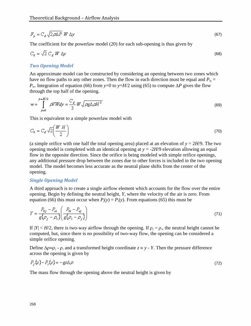
Theoretical Background – Airflow Analysis
268
(67)
The coefficient for the powerlaw model (20) for each sub-opening is thus given by
(68)
Two Opening Model
An approximate model can be constructed by considering an opening between two zones which
have no flow paths to any other zones. Then the flow in each direction must be equal and P0j =
P0i. Integration of equation (66) from y=0 to y=H/2 using (65) to compute P gives the flow
through the top half of the opening.
(69)
This is equivalent to a simple powerlaw model with
(70)
(a simple orifice with one half the total opening area) placed at an elevation of y = 2H/9. The two
opening model is completed with an identical opening at y = -2H/9 elevation allowing an equal
flow in the opposite direction. Since the orifice is being modeled with simple orifice openings,
any additional pressure drop between the zones due to other forces is included in the two opening
model. The model becomes less accurate as the neutral plane shifts from the center of the
opening.
Single Opening Model
A third approach is to create a single airflow element which accounts for the flow over the entire
opening. Begin by defining the neutral height, Y, where the velocity of the air is zero. From
equation (66) this must occur when Pj(y) = Pi(y). From equations (65) this must be
(71)
If |Y| < H/2, there is two-way airflow through the opening. If j = i, the neutral height cannot be
computed, but, since there is no possibility of two-way flow, the opening can be considered a
simple orifice opening.
Define j - i and a transformed height coordinate z y - Y. Then the pressure difference
across the opening is given by
(72)
The mass flow through the opening above the neutral height is given by
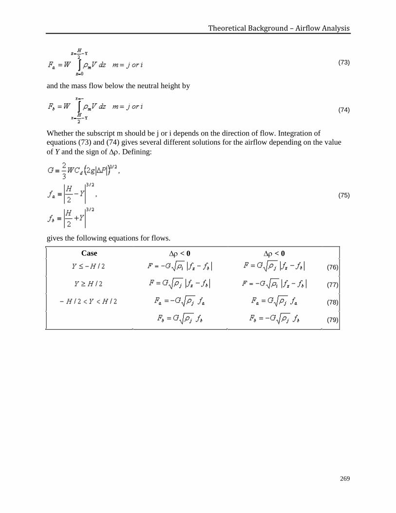
Theoretical Background – Airflow Analysis
269
(73)
and the mass flow below the neutral height by
(74)
Whether the subscript m should be j or i depends on the direction of flow. Integration of
equations (73) and (74) gives several different solutions for the airflow depending on the value
of Y and the sign of . Defining:
(75)
gives the following equations for flows.
Case < 0 < 0
(76)
(77)
(78)
(79)
References
270
8 REFERENCES
ACM 1982. ACM-Transactions. Mathematical Software, Vol.8, No. 2, June 1982, p. 190.
Achakji, G.Y. & G.T. Tamura, 1988. "Pressure Drop Characteristics of Typical Stairshafts in
High rise Buildings," ASHRAE Transactions, 94(1): 1223-1236.
AIVC 1991. Technical Note AIVC 34 – Airflow Patterns within Buildings: Measurement
Techniques, Coventry UK.
ASHRAE 1993. ASHRAE Handbook - 1993 Fundamentals, Atlanta GA.
ASHRAE 1999a. Method of Testing General Ventilation Air-Cleaning Devices for Removal
Efficiency by Particle Size (ANSI approved). Standard 52.2-1999. Atlanta, GA.
ASHRAE 1999b. ASHRAE Handbook - HVAC Applications, Atlanta GA.
ASHRAE 2001. ASHRAE Handbook - 2001 Fundamentals, Atlanta GA.
ASHRAE 2002. Duct Fitting Database, v. 2.2.5, Atlanta GA.
ASHRAE 2004. ASHRAE Handbook - HVAC Systems and Equipment, Atlanta GA.
ASHRAE 2005. ASHRAE Handbook - 2005 Fundamentals, Atlanta GA.
ASTM 1999. Standard Test Method for Determining Air Leakage Rate by Fan Pressurization.
Standard E779-99. American Society for Testing and Materials, West Conshohocken, PA.
Axley, J.W. 1987. "Indoor Air Quality Modeling Phase II Report", NBSIR 87-3661, National
Bureau of Standards (U.S.).
Axley, J.W. 1988. "Progress Toward a General Analytical Method for Predicting Indoor Air
Pollution in Buildings, Indoor Air Quality Modeling Phase III Report", NBSIR 88-3814,
National Bureau of Standards (U.S.).
Axley, J.W. 1991. "Adsorption Modeling for Building Contaminant Dispersal Analysis", Indoor
Air, 1:147-171.
Axley, J.W. 1995. "New Mass Transport Elements and Components for the NIST IAQ Model",
NIST GCR 95-676, National Institute of Standards and Technology(U.S.).
Axley, J. W. 2001. Residential Passive Ventilation Systems: Evaluation and Design. AIVC
Technical Note 54. International Energy Agency, Coventry.
Baker, P.H., S. Sharples, & I.C. Ward. 1987. "Air Flow through Cracks," Building and
Environment, Pergamon, 22(4): 293-304.
Barakat, S.A. 1987. "Inter-zone Convective Heat Transfer in Buildings: a Review," ASME
Journal of Solar Engineering, Vol. 109, May.
Blevins, R.D. 1984. Applied Fluid Dynamics Handbook, New York: Van Nostrand Reinhold.
Brown, W.G., & K.R. Solvason. 1962. "Natural Convection through Rectangular Openings in
Partitions - 1: Vertical Partitions," International Journal of Heat and Mass Transfer, Vol. 5, pp.
859-867.
Clarke, J.A. 1985. Energy Simulation in Building Design, Adam Hilger Ltd., Briston and Boston,
p 204.

References
271
Conte, S.D. and C. de Boor. 1972. Elementary Numerical Analysis, McGraw Hill, New York
NY.
Dennis, J.E., Jr. and R.B. Schnabel. 1996. Numerical Methods for Unconstrained Optimization
and Nonlinear Equations, Society for Industrial and Applied Mathematics, Philadelphia.
Dhatt, G., G. Touzot, & G. Catin. 1984. The Finite Element Method Displayed, John Wiley &
Sons, New York.
Dols, W.S., Walton G.N., & Denton, K.R. 2000. "CONTAMW 1.0 User Manual", NISTIR 6476,
National Institute of Standards and Technology.
Dols, W.S., L. Wang, S.J. Emmerich, B.J. Polidoro. 2014. "Development and application of an
updated whole-building coupled thermal, airflow and contaminant transport simulation program
(TRNSYS/CONTAM)." Journal of Building Performance Simulation: 1-21.
Dols, W.S., S.J. Emmerich, B.J. Polidoro. 2014. Evaluating Building Ventilation Strategies
Using Newly-Developed TRNSYS/CONTAM Simulation Capabilities. 2014 CIBSE ASHRAE
Technical Symposium. Dublin, Ireland, CIBSE.
Emmerich, S.J. and A.K. Persily. 1996. "Multizone Modeling of Three Residential Indoor Air
Quality Control Options", NISTIR 5801, National Institute of Standards and Technology.
Emmerich, S.J. and A.K. Persily. 1998. "Energy Impacts of Infiltration and Ventilation in U.S.
Office Buildings Using Multizone Airflow Simulation" Proceeding of IAQ and Energy 98. New
Orleans, Louisiana: ASHRAE.
Emmerich, S.J. and S.J. Nabinger. 2000. "Measurement and Simulation of the IAQ Impact of
Particle Air Cleaners in a Single-Zone Building", NISTIR 6461, National Institute of Standards
and Technology.
Emmerich, S.J., JE Gorfain, M. Huang, C. Howard-Reed. 2003. "Air and Pollutant Transport
from Attached Garages to Residential Living Spaces," NISTIR 7072, National Institute of
Standards and Technology, Gaithersburg, MD. December 2003.
EPA 1989. Exposure Factors Handbook. Publication number EPA/600/8 89/043.
Fang, J.B. and A.K. Persily. 1995. "Computer Simulations of Airflow and Radon Transport in
Four Large Buildings", NISTIR 5611, National Institute of Standards and Technology.
Feustel, H.E. and A. Rayner-Hooson (Eds). 1990. "COMIS Fundamentals", Lawrence Berkeley
Laboratory, report LBL-28560.
Feustel, H.E. and J. Dieris. 1992. "A survey of airflow models for multizone structures", Energy
and Buildings, Vol 18, pp. 79-100.
Guglielmetti, R., D. Macumber, N. Long. 2011. OpenStudio: An Open Source Integrated
Analysis Platform. Building Simulation 2011. Sydney, IBPSA.
Hindmarsh, A.C., R. Serban. 2012. User Documentation for CVODE v2.7.0. UCRL-SM-20818.
Lawrence Livermore National Laboratory.
Howard-Reed, C., Begley, E., Polidoro, B., Dols, W.S. "VOC Source Emission Rate Databases:
Model Input and Data Format Issues," ASTM Conference on Indoor Emissions Testing: Methods
and Interpretation, October 2004.

References
272
Howard-Reed, C. and Polidoro, B. "Database Development for Modeling Emissions and Control
of Air Pollutants from Consumer Products, Cooking, and Combustion," NISTIR 7364, 2006.
Isaacs, L.T. and K.G. Mills. 1980. "Linear Theory Methods for Pipe Network Analysis", Journal
of the Hydraulics Division, Proceedings ASCE, Vol. 106, pp. 1191-1201. (See also author's
closure, 1982, Vol. 108, p. 153).
Klote, J.H. 1982. "A Computer Program for Analysis of Smoke Control Systems", NBSIR 82-
2512, National Bureau of Standards (U.S.).
Klote, J.H. and J.A. Milke. 2002. Principles of Smoke Management, ASHRAE, Atlanta GA.
Klote, J.H., J.A. Milke, P.G. Turnbull, A. Kashef, M.J. Ferreira. 2012. Handbook of Smoke
Control Engineering. Atlanta, GA, American Society of Heating, Refrigerating and Air-
Conditioning Engineers.
Kowalski, W., W. Bahnfleth, D. Witham, B. Severin, and T. Whittam. 2000. Mathematical
modeling of ultraviolet germicidal irradiation for air disinfection. Quantitative Microbiology.
2(3): p. 249-270.
Lau, J. 2009. Lamp and In-Duct Device Modeling for UVGI System Performance Prediction,
Ph.D. Thesis in Architectural Engineering. 2009. The Pennsylvania State University.
Lau, J., W. Bahnfleth, and J. Freihaut. 2009. Estimating the effects of ambient conditions on the
performance of UVGI air cleaners. Building and Environment. 44(7): p. 1362-1370.
Lee, B. and W.P. Bahnfleth. 2013. Effects of installation location on performance and economics
of in-duct ultraviolet germicidal irradiation systems for air disinfection. Building and
Environment. 67(0): p. 193-201.
Lorenzetti, D. M., W.S. Dols, A.K. Persily, M.D. Sohn. 2013. "A stiff, variable time step
transport solver for CONTAM." Building and Environment 67(0): 260-264.
MODELISAR. 2010. Functional Mock-up Interface for Co-Simulation. ITEA2-07006.
MODELISAR consortium. https://www.fmi-standard.org.
MODELISAR. 2010. Functional Mock-up Interface for Model Exchange. ITEA2-07006.
MODELISAR consortium. https://www.fmi-standard.org.
Musser, A. and G. Yuill. 1999. "Comparison of Residential Air Infiltration Rates Predicted by
Single-Zone and Multizone Models," ASHRAE Transactions. Vol. 105(Part 1).
Musser, A. 2000. "Multizone Modeling as an Indoor Air Quality Design Tool", Proceedings of
Healthy Buildings 2000. Espoo, Finland.
Nouidui, T. S., M. Wetter, W. Zuo. 2014. "Functional mock-up unit for co-simulation import in
EnergyPlus." Journal of Building Performance Simulation 7(3): 1-11.
NREL. 2015. "OpenStudio." Retrieved June 5, 2015, from https://www.openstudio.net/. National
Renewable Energy Laboratory. Golden, CO.
Osborne, W.C., 1977. Fans, 2nd edition, Pergamon Press.
Patankar, S.V,. 1980. Numerical Heat Transfer and Fluid Flow, Hemisphere Publishing. ISBN:
0-89116-522-3.

References
273
Persily, A.K. 1998. "A Modeling Study of Ventilation, IAQ and Energy Impacts of Residential
Mechanical Ventilation", NISTIR 6162, National Institute of Standards and Technology.
Persily, A.K. and S.R. Martin 2000. "A Modeling Study of Ventilation in Manufactured
Houses", NISTIR 6455, National Institute of Standards and Technology.
Persily, A.K. and E.M. Ivy. 2001. "Input Data for Multizone Airflow and IAQ Analysis",
NISTIR 6585, National Institute of Standards and Technology.
Press, W.H., S.A. Teukolsky, W.T. Vetterling & B.P. Flannery. 1992. Numerical Recipes in C:
the Art of Scientific Computing, Second Edition, Cambridge University Press.
Roulet, C-A, and L. Vandaele, Airflow Patterns Within Buildings Measurement Techniques, The
Air Infiltration and Ventilation Centre, Technical Note 34, 1991, pp. iii.10 and iv.3.
Stoecker, W.F. and P.A. Stoecker. 1989. Microcomputer Control of Thermal and Mechanical
Systems. Van Nostrand Reinhold, New York.
U.S. DOE. 2013. EnergyPlus External Interface(s) Application Guide (version 8.2). Champaign,
IL, University of Illinois.
Versteeg, H.K., and W. Malalasekera, 1995. An Introduction to Computational Fluid Dynamics :
The Finite Volume Method, Pearson Education Ltd. ISBN: 0-582-21884-5.
Walker, I.S., and D.J. Wilson 1994. "Practical Methods for Improving Estimates of Natural
Ventilation Rates", Proceedings 15th
AIVC Conference, Vol. 2, pp. 517-525.
Walton, G.N. 1989a. "AIRNET - A Computer Program for Building Airflow Network
Modeling", NISTIR 89-4072, National Institute of Standards and Technology.
Walton, G.N., 1989b. "Airflow Network Models for Element-Based Building Airflow
Modeling", ASHRAE Transactions, Vol. 95, Pt. 2.
Walton, G.N. 1997. "CONTAM96 User Manual", NISTIR 6056, National Institute of Standards
and Technology.
Walton, G.N. and W.S. Dols. 2003. "CONTAM 2.1 Supplemental User Guide and Program
Documentation," NISTIR 7049, National Institute of Standards and Technology.
Wang, L. (2007). Coupling of Multizone and CFD Programs for Building Airflow and
Contaminant Transport Simulations. Lafayette, Purdue University. PhD Thesis.
Wang, L. and Q. Chen (2007). "Theoretical and Numerical Studies of Coupling Multizone and
CFD Models for Building Air Distribution Simulations." Indoor Air 17: 348-361.
Wang, L. and Q. Chen (2007). "Validation of a Coupled Multizone and CFD Program for
Building Airflow and Contaminant Transport Simulations." HVAC&R Research 13(2): 267-281.
Wang, L. (2008). "Applications of a Coupled Multizone and CFD Model to Calculate Airflow
and Contaminant Dispersion in Built Environment for Emergency Management." HVAC&R
Research 14(6): 925-939.
Wang, L. (2010). "Using CFD Capabilities of CONTAM 3.0 for Simulating Airflow and
Contaminant Transport in and around Buildings." HVAC&R Research 16(6).
Weber, D.D, and R.J. Kearney, 1980. Natural Convective Heat Transfer Through an Aperture in
Passive Solar Heated Buildings, 5th National Passive Solar Conference, pp. 1037-1041.
References
274
Wetter, M. 2011. "Co-Simulation of Building Energy and Control Systems with the Building
Controls Virtual Test Bed." Journal of Building Performance Simulation 4 (3):185-203.
Wang, L., W.S. Dols and Q. Chen. 2010. An Introduction to the CFD Capabilities in CONTAM
3.0. SimBuild 2010 - Fourth International Conference of IBPSA-USA. New York City, NY,
IBPSA.
Wen, C.Y. and L.T. Fan, 1975. Models for Flow Systems and Chemical Reactors, Marcel
Dekker, Inc. New York. ISBN: 0-8247-6346-7.
Wray, C.P. and G.K. Yuill. 1993. "An Evaluation of Algorithms for Analyzing Smoke Control
Systems", ASHRAE Transactions, Vol. 99, Pt. 1.
Appendix A - PRJ File Format
275
APPENDIX A - PRJ FILE FORMAT
CONTAM consists of two separate programs: ContamW provides the graphic user interface for
describing the building and viewing simulation results; ContamX performs the simulation.
"Project" files (.PRJ extension) provide input to both ContamW and ContamX. Project files are
created by the functions in file prjsave.c in ContamW and read by the functions in file prjread.c
in ContamW and ContamX. The project file contains some information that is used only by
ContamW and not by ContamX, e.g., input units and the SketchPad display data. These data are
read when the macro name CTMW is defined to be 1, and they are not read when it is defined to
be 0.
Most of the data are read into structures that are defined in the files contam.h and celmts.h for
ContamW and files simdat.h and selmts.h for ContamX. Some data are read into global variables
that are defined in cglob.h and cxtrn.h for ContamW and sglob.h and sxtrn.h for ContamX. These
variables are indicated by a leading underscore, _, in their name.
One important feature of the project files is the tremendous variety of data stored. It has been
divided into sections grouping similar kinds of data, or objects, together. Each section is
terminated with the special value –999 which serves as a check for some reading errors. Within
each section there are usually multiple objects, each stored into an individual structure. Such a
section begins with the number of objects and starts the data for each object with a sequence
number that serves to check for reading errors. These objects may be ordered as arrays when the
total number is constant, or as linked lists to allow the number to vary.
In the following material individual variables are briefly described. Units are indicated within
brackets, [ ]. The type of variable is in parentheses (matching the definitions in the include file
types.h).
I1 – a one-byte signed integer (C type "char")
I2 – a two-byte signed integer (C type "short")
I4 – a four-byte signed integer (C type "long")
IX – a default length signed integer (C type "int")
UX – a default length unsigned integer (C type "unsigned")
R4 – a four-byte real (C type "float")
Variables used only by ContamW are indicated by {W}. Items that appear in red are the most
recently modified items including those whose data size has been increased from 2-bytes to 4-
bytes to allow for an increased number of building components. This change took place between
versions 2.3 and 2.4.
Comments are included in the project file to make it somewhat human-readable. The
exclamation mark, "!" serves as a comment character. Anything after an exclamation mark to
the end of the line is not read by the input processor. Any user-defined comments within a PRJ
file will not be maintained when the file is saved by ContamW.
Appendix A - PRJ File Format
276
Sections of the PRJ File
Section 1: Project, Weather, Simulation, and Output Controls
Section 2: Species and Contaminants
Section 3: Level and Icon Data
Section 4: Day Schedules
Section 5: Week Schedules
Section 6: Wind Pressure Profiles
Section 7: Kinetic Reactions
Section 8a: Filter Elements
Section 8b: Filters
Section 9: Source/Sink Elements
Section 10: Airflow Elements
Section 11: Duct Elements
Section 12a: Control Super Elements
Section 12b: Control Nodes
Section 13: Simple Air Handling System (AHS)
Section 14: Zones
Section 15: Initial Zone Concentrations
Section 16: Airflow Paths
Section 17: Duct Junctions
Section 18: Initial Junction Concentrations
Section 19: Duct Segments
Section 20: Source/Sinks
Section 21: Occupancy Schedules
Section 22: Exposures
Section 23: Annotations
Section 1: Project, Weather, Simulation, and Output Controls
The initial section of the project file is read by the run_read( ) function and saved by the
run_save( ) function.
The first line of the project file identifies the source program:
_string[] // program name "ContamW" (I1)
_string[] // program version "3.2" (I1)
_echo // > 0 echo input files, > 1 echo bridge messages to the log file (I2)
The second line is a user-defined description of the project:
_prjdesc[] // (unused) project description (I1) {W}
The next line sets the following miscellaneous values:
_skheight // total SketchPad height [cells] (I2) {W}
_skwidth // total SketchPad width [cells] (I2) {W}
_def_units // default units: 0 = SI, 1 = US (I2) {W}
_def_flows // default flows: 0 = mass, 1 = volume (I2) {W}
_def_T // default temperature for zones [K] (R4) {W}
_udefT // units for temperature (I2) {W}
_rel_N // angle to true north [degrees] (R4) {W}
_wind_H // elevation for reference wind speed [m] (R4) {W}
Appendix A - PRJ File Format
277
_uwH // units for _wind_H (I2) {W}
_wind_Ao // local terrain constant (R4) {W}
_wind_a // velocity profile exponent (R4) {W}
The next line provides SketchPad pseudo-geometry information: {CONTAM 3.1}
scale // cell scaling factor (R4)
uScale // units of scaling factor: 0 = m, 1 = ft (I2)
orgRow // row of origin (I2)
orgCol // column of origin (I2)
invYaxis // 0 = positive above origin, 1 = negative above origin (I2)
showGeom // 0/1 = show pseudo-geometry info in status bar (I2)
The next line defines the weather (WTHDAT) for steady-state simulation in ContamX:
Tambt // ambient temperature [K] (R4)
barpres // barometric pressure [Pa] NOT corrected to sea level (R4)
windspd // wind speed [m/s] (R4)
winddir // wind direction: 0 = N, 90 = E, 180 = S, ...; (R4)
relhum // relative humidity: 0.0 to 1.0 (R4)
daytyp // type of day (1-12) (I2)
uTa // units for Tambt (I2) {W}
ubP // units for barpres (I2) {W}
uws // units for windspd (I2) {W}
uwd // units for winddir (I2) {W}
The next line defines weather data (WTHDAT) for the wind pressure test in ContamW:
Tambt // ambient temperature [K] (R4) {W}
barpres // barometric pressure [Pa] NOT corrected to sea level (R4) {W}
windspd // wind speed [m/s] (R4) {W}
winddir // wind direction: 0 = N, 90 = E, 180 = S, ...; (R4) {W}
relhum // relative humidity: 0.0 to 1.0 (R4) {W}
daytyp // type of day (1-12) (I2) {W}
uTa // units for Tambt (I2) {W}
ubP // units for barpres (I2) {W}
uws // units for windspd (I2) {W}
uwd // units for winddir (I2) {W}
The next four lines define the weather, contaminant and controls files, respectively:
_WTHpath[_MAX_PATH] // full name of weather file (I1)
_CTMpath[_MAX_PATH] // full name of contaminant file (I1)
_CVFpath[_MAX_PATH] // full name of continuous values file (I1)
_DVFpath[_MAX_PATH] // full name of discrete values file (I1)
The following lines define path location data (PLDDAT) for the creating the WPC file:
three lines for file paths and WPC description:
WPCfile[_MAX_PATH] // full name of WPC file (I1)
EWCfile[_MAX_PATH] // full name of EWC data source file (I1) {W}
WPCdesc[] // WPC description (I1) {W}
next a line describing reference coordinates:
X0 // X-value of ContamW origin in EWC coordinates [m] (R4) {W}
Y0 // Y-value of ContamW origin in EWC coordinates [m] (R4) {W}

Appendix A - PRJ File Format
278
Z0 // Z-value of ContamW origin in EWC coordinates [m] (R4) {W}
angle // Rotation of ContamW relative to EWC coordinates (R4) {W}
u_XYZ // units of coordinates (I2) {W}
then some EWC to WPC conversion parameters:
epsPath // tolerance for matching path locations [-] (R4) {W}
epsSpcs // tolerance for matching species [-] (R4) {W}
tShift // time shift of EWC data {W} [s] (hh:mm:ss IX) {W}
dStart // date WPC data starts (I2) {W}
dEnd // date WPC data ends (I2) {W}
_useWPCwp // if true, use WPC file wind pressures (I2)
_useWPCmf // if true, use WPC file mass fractions (I2)
wpctrig // 0/1 = trigger airflow calculation by WPC data (I2) {CONTAM 3.1}
The next line defines the location (LOCDAT) (for future use with thermal simulation):
latd // latitude (degrees: north +, south -) (R4)
lgtd // longitude (degrees: east +, west -) (R4)
Tznr // time zone (Greenwich = 0, Eastern = -5, etc.) (R4)
altd // elevation above sea level [m] (R4)
Tgrnd // ground temperature [K] (R4)
utg // units for ground temperatures (I2)
u_a // units for elevation (I2)
The remaining data is stored in the run control (RCDAT) structure. In ContamX some values
may be transferred to other variables before being used. The next two lines control the airflow
simulation – first the nonlinear part:
sim_af // airflow simulation: 0 = steady, 1 = dynamic (I2)
afcalc // N-R method for non-linear eqns: 0 = SUR, 1 = STR (I2)
afmaxi // maximum number of N-R iterations (I2)
afrcnvg // relative airflow convergence factor (R4)
afacnvg // absolute airflow convergence factor [1/s] (R4)
afrelax // flow under-relaxation coefficient (for SUR) (R4)
uac2 // units for afacnvg (I2)
Pres // pressure test pressure (R4) {Contam 2.4}
uPres // units of Pres (I2) {Contam 2.4}
and then the linear part:
afslae // method for linear equations: 0 = SKY, 1 = PCG (I2)
afrseq // if true, resequence the linear equations (I2)
aflmaxi // maximum number of iterations (PCG) (I2)
aflcnvg // relative convergence factor for (PCG) (R4)
aflinit // if true, do linear airflow initialization (I2)
Tadj // if true, use temperature adjustment (I2)
The next four lines control the linear solver for contaminant calculations:
first for cyclic simulation:
sim_mf // mass fraction (contaminant) simulation:
// 0 = none, 1 = steady, 2 = transient, 3 = cyclic (I2)
ccmaxi // simulation: maximum number of cyclic iterations (I2)
ccrcnvg // relative convergence factor (R4)
Appendix A - PRJ File Format
279
ccacnvg // absolute convergence factor [kg/kg] (R4)
ccrelax // (unused) over-relaxation coefficient (R4)
uccc // units for ccacnvg (I2)
then for non-trace contaminants:
mfnmthd // simulation: 0 = SKY, 1 = BCG, 2 = SOR, 3 = LU (I2)
mfnrseq // if true, resequence the linear equations (I2)
mfnmaxi // maximum iterations (I2)
mfnrcnvg // desired relative convergence (R4)
mfnacnvg // desired absolute convergence (R4)
mfnrelax // relaxation coefficient (R4)
mfngamma // trapezoidal integration factor (R4)
uccn // units for mfnacnvg (I2)
then for trace contaminants:
mftmthd // 0 = SKY, 1 = BCG, 2 = SOR, 3 = LU (I2)
mftrseq // if true, resequence the linear equations (I2)
mftmaxi // maximum iterations (I2)
mftrcnvg // desired relative convergence (R4)
mftacnvg // desired absolute convergence (R4)
mftrelax // relaxation coefficient (R4)
mftgamma // trapezoidal integration factor (R4)
ucct // units for mftacnvg (I2)
then for CVODE contaminant solver: {CONTAM 3.1}
mfvmthd // 0 = SKY, 2 = SOR, 3 = LU (1 n/a) (I2)
mfvrseq // if true, resequence the linear equations (I2)
mfvmaxi // maximum iterations (I2)
mfvrcnvg // desired relative convergence (R4)
mfvacnvg // desired absolute convergence (R4)
mfvrelax // relaxation coefficient (R4)
uccv // units for mfvacnvg (I2)
The next line sets the integration method and short time step contaminant calculation
parameters:
mf_solver // mass fraction integration method: {3.1}
// 0=trapezoid, 1=STS, 2=CVODE (I2)
sim_1dz // if true, use 1D zones (I2)
sim_1dd // if true, use 1D ducts (I2)
celldx // default length of duct cells for C-D model [m] (R4)
sim_vjt // if true, compute variable junction temperatures (I2)
udx // units of celldx (I2)
The next line contains CVODE contaminant solver parameters: {CONTAM 3.1}
cvode_mth // 0 = am, 1 = bdf (I2)
cvode_rcnvg // relative convergence factor(R4)
cvode_acnvg // absolute convergence factor(R4)
cvode_dtmax // maximum time step (R4)
The next line contains density control parameters:
tsdens // (0/1) vary density during time step (I2)

Appendix A - PRJ File Format
280
tsrelax // (inactive) under-relaxation factor for calculating dM/dt (R4)
tsmaxi // maximum number of iterations for density changes (I2)
cnvgSS // (0/1) converge density in steady state init (I1) {2.4b}
densZP // (0/1) density = f(zone pressure) (I1) {2.4b, 3.1}
stackD // (0/1) density varies hydrostatically (I1) {2.4b, 3.1}
dodMdt // (0/1) include dM/dt in airflow calc (I1) {2.4b, 3.1}
The next line sets the dates, times, and time steps for simulation:
date_st // day-of-year to start steady simulation (mmmdd IX)
time_st // time-of-day to start steady simulation (hh:mm:ss I4)
date_0 // day-of-year to start transient simulation (mmmdd IX)
time_0 // time-of-day to start transient simulation (hh:mm:ss I4)
date_1 // day-of-year to end transient simulation (mmmdd IX)
time_1 // time-of-day to end transient simulation (hh:mm:ss I4)
time_step // simulation time step [s] (hh:mm:ss IX)
time_list // simulation output (results) time step [s] (hh:mm:ss IX)
time_scrn // simulation status time step [s] (up to 1 day) (hh:mm:ss I4)
The next line controls the use of the restart file:
restart // use restart file (I2)
rstdate // restart date (mmmdd IX)
rsttime // restart time (hh:mm:ss I4)
The next line controls output of simulation result files.
_list // data dump parameter (I2)
// > 0 dump matrix analysis,
// = 2 dump SIM file output,
// > 2 dump lognotes.
_doDlg // (0/1) ContamX will display dialog box (I1)
_pfsave // (0/1) save path flow results to SIM file (I1)
_zfsave // (0/1) save zone flow results to SIM file (I1)
_zcsave // (0/1) save mass fraction results to SIM file (I1)
_achvol // (0/1) ACH based on true volumes instead of std volumes
_achsave // (0/1) save building air exchange rate transient data
_abwsave // (0/1) save air exchange rate box-whisker data
_cbwsave // (0/1) save contaminant box-whisker data
_expsave // (0/1) save exposure transient data
_ebwsave // (0/1) save exposure box-whisker data
_zaasave // (0/1) save zones age-of-air transient data
_zbwsave // (0/1) save zones age-of-air box-whisker data
The next line controls output of more simulation result files: {CONTAM 3.1}
rzfsave // (0/1) save binary zone flow file
rzmsave // (0/1) save binary avg zone mass fraction file
rz1save // (0/1) save binary 1D zone cell mass fraction file
csmsave // (0/1) save text contaminant summary file
srfsave // (0/1) save text surface result file
logsave // (0/1) save text controls log file
The next line controls output of more simulation result files: {CONTAM 3.2}
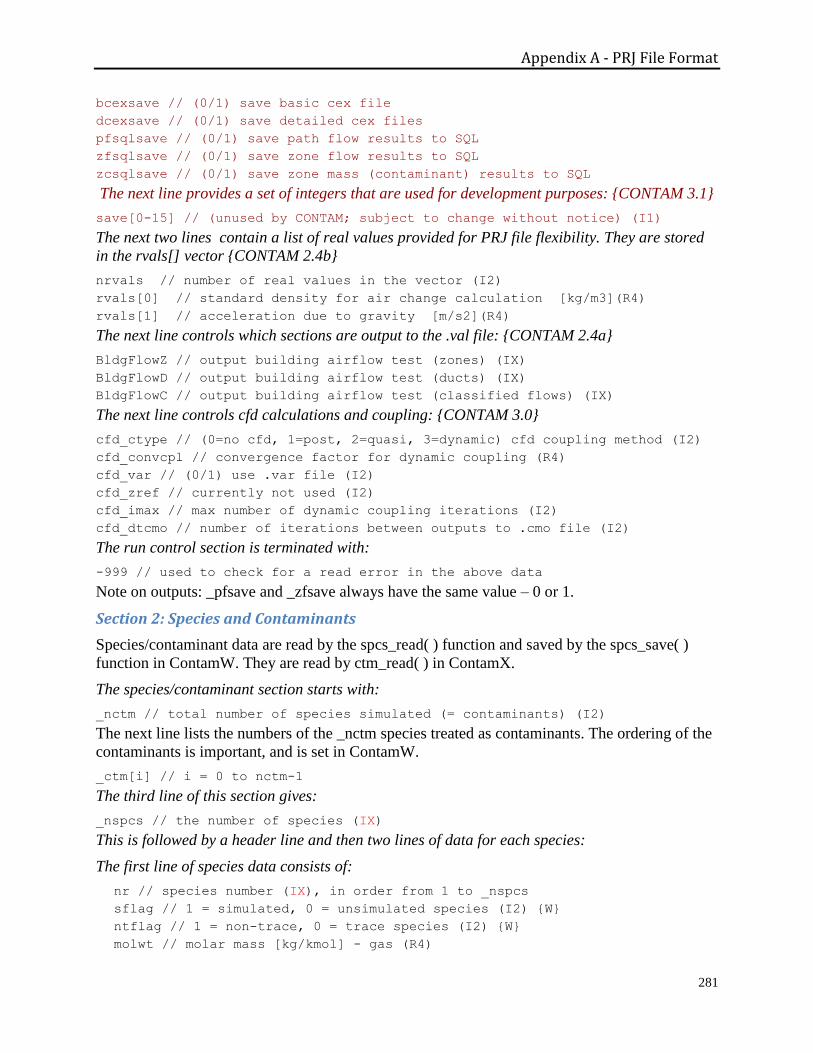
Appendix A - PRJ File Format
281
bcexsave // (0/1) save basic cex file
dcexsave // (0/1) save detailed cex files
pfsqlsave // (0/1) save path flow results to SQL
zfsqlsave // (0/1) save zone flow results to SQL
zcsqlsave // (0/1) save zone mass (contaminant) results to SQL
The next line provides a set of integers that are used for development purposes: {CONTAM 3.1}
save[0-15] // (unused by CONTAM; subject to change without notice) (I1)
The next two lines contain a list of real values provided for PRJ file flexibility. They are stored
in the rvals[] vector {CONTAM 2.4b}
nrvals // number of real values in the vector (I2)
rvals[0] // standard density for air change calculation [kg/m3](R4)
rvals[1] // acceleration due to gravity [m/s2](R4)
The next line controls which sections are output to the .val file: {CONTAM 2.4a}
BldgFlowZ // output building airflow test (zones) (IX)
BldgFlowD // output building airflow test (ducts) (IX)
BldgFlowC // output building airflow test (classified flows) (IX)
The next line controls cfd calculations and coupling: {CONTAM 3.0}
cfd_ctype // (0=no cfd, 1=post, 2=quasi, 3=dynamic) cfd coupling method (I2)
cfd_convcpl // convergence factor for dynamic coupling (R4)
cfd_var // (0/1) use .var file (I2)
cfd_zref // currently not used (I2)
cfd_imax // max number of dynamic coupling iterations (I2)
cfd_dtcmo // number of iterations between outputs to .cmo file (I2)
The run control section is terminated with:
-999 // used to check for a read error in the above data
Note on outputs: _pfsave and _zfsave always have the same value – 0 or 1.
Section 2: Species and Contaminants
Species/contaminant data are read by the spcs_read( ) function and saved by the spcs_save( )
function in ContamW. They are read by ctm_read( ) in ContamX.
The species/contaminant section starts with:
_nctm // total number of species simulated (= contaminants) (I2)
The next line lists the numbers of the _nctm species treated as contaminants. The ordering of the
contaminants is important, and is set in ContamW.
_ctm[i] // i = 0 to nctm-1
The third line of this section gives:
_nspcs // the number of species (IX)
This is followed by a header line and then two lines of data for each species:
The first line of species data consists of:
nr // species number (IX), in order from 1 to _nspcs
sflag // 1 = simulated, 0 = unsimulated species (I2) {W}
ntflag // 1 = non-trace, 0 = trace species (I2) {W}
molwt // molar mass [kg/kmol] - gas (R4)
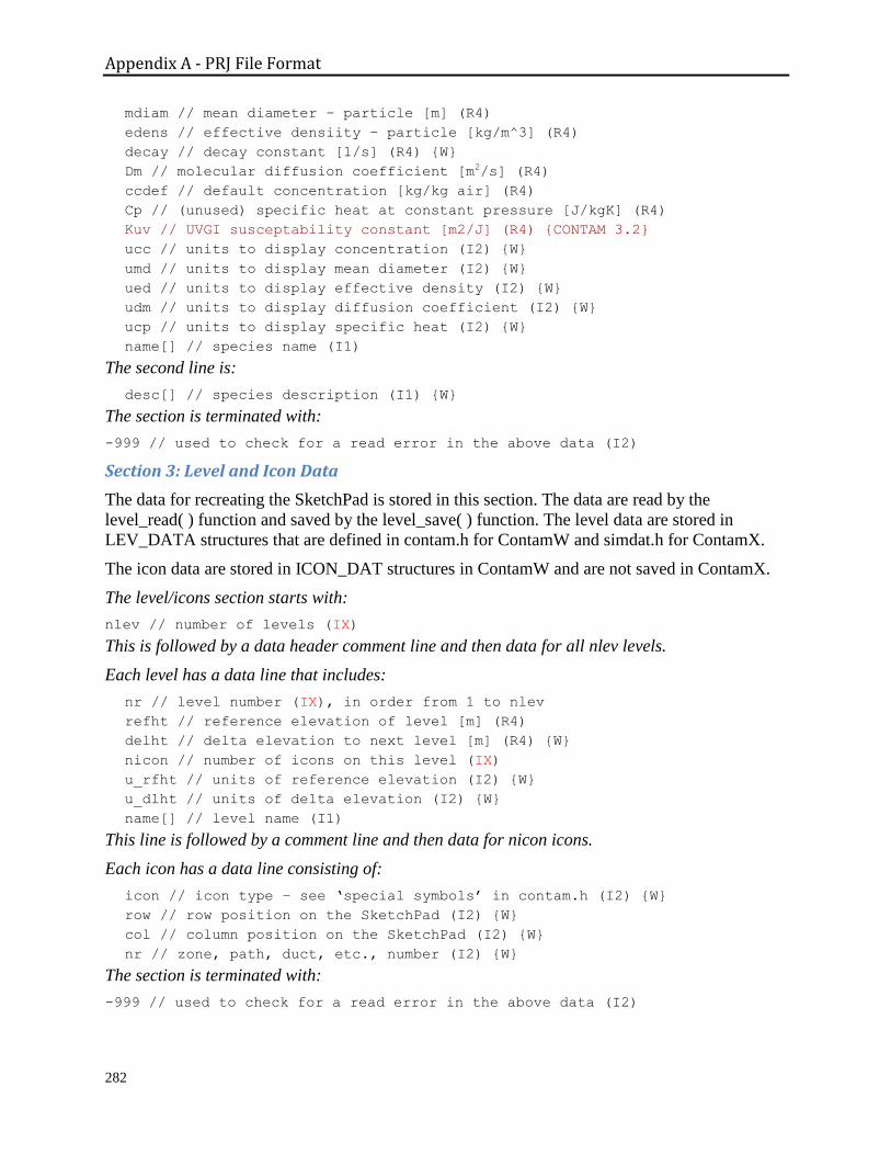
Appendix A - PRJ File Format
282
mdiam // mean diameter – particle [m] (R4)
edens // effective densiity – particle [kg/m^3] (R4)
decay // decay constant [1/s] (R4) {W}
Dm // molecular diffusion coefficient [m2/s] (R4)
ccdef // default concentration [kg/kg air] (R4)
Cp // (unused) specific heat at constant pressure [J/kgK] (R4)
Kuv // UVGI susceptability constant [m2/J] (R4) {CONTAM 3.2}
ucc // units to display concentration (I2) {W}
umd // units to display mean diameter (I2) {W}
ued // units to display effective density (I2) {W}
udm // units to display diffusion coefficient (I2) {W}
ucp // units to display specific heat (I2) {W}
name[] // species name (I1)
The second line is:
desc[] // species description (I1) {W}
The section is terminated with:
-999 // used to check for a read error in the above data (I2)
Section 3: Level and Icon Data
The data for recreating the SketchPad is stored in this section. The data are read by the
level_read( ) function and saved by the level_save( ) function. The level data are stored in
LEV_DATA structures that are defined in contam.h for ContamW and simdat.h for ContamX.
The icon data are stored in ICON_DAT structures in ContamW and are not saved in ContamX.
The level/icons section starts with:
nlev // number of levels (IX)
This is followed by a data header comment line and then data for all nlev levels.
Each level has a data line that includes:
nr // level number (IX), in order from 1 to nlev
refht // reference elevation of level [m] (R4)
delht // delta elevation to next level [m] (R4) {W}
nicon // number of icons on this level (IX)
u_rfht // units of reference elevation (I2) {W}
u_dlht // units of delta elevation (I2) {W}
name[] // level name (I1)
This line is followed by a comment line and then data for nicon icons.
Each icon has a data line consisting of:
icon // icon type – see ‘special symbols’ in contam.h (I2) {W}
row // row position on the SketchPad (I2) {W}
col // column position on the SketchPad (I2) {W}
nr // zone, path, duct, etc., number (I2) {W}
The section is terminated with:
-999 // used to check for a read error in the above data (I2)
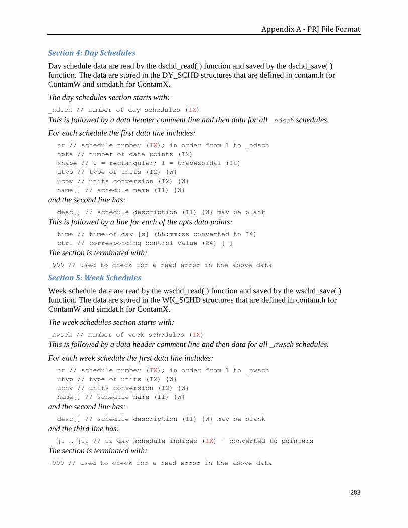
Appendix A - PRJ File Format
283
Section 4: Day Schedules
Day schedule data are read by the dschd_read( ) function and saved by the dschd_save( )
function. The data are stored in the DY_SCHD structures that are defined in contam.h for
ContamW and simdat.h for ContamX.
The day schedules section starts with:
_ndsch // number of day schedules (IX)
This is followed by a data header comment line and then data for all _ndsch schedules.
For each schedule the first data line includes:
nr // schedule number (IX); in order from 1 to _ndsch
npts // number of data points (I2)
shape // 0 = rectangular; 1 = trapezoidal (I2)
utyp // type of units (I2) {W}
ucnv // units conversion (I2) {W}
name[] // schedule name (I1) {W}
and the second line has:
desc[] // schedule description (I1) {W} may be blank
This is followed by a line for each of the npts data points:
time // time-of-day [s] (hh:mm:ss converted to I4)
ctrl // corresponding control value (R4) [-]
The section is terminated with:
-999 // used to check for a read error in the above data
Section 5: Week Schedules
Week schedule data are read by the wschd_read( ) function and saved by the wschd_save( )
function. The data are stored in the WK_SCHD structures that are defined in contam.h for
ContamW and simdat.h for ContamX.
The week schedules section starts with:
_nwsch // number of week schedules (IX)
This is followed by a data header comment line and then data for all _nwsch schedules.
For each week schedule the first data line includes:
nr // schedule number (IX); in order from 1 to _nwsch
utyp // type of units (I2) {W}
ucnv // units conversion (I2) {W}
name[] // schedule name (I1) {W}
and the second line has:
desc[] // schedule description (I1) {W} may be blank
and the third line has:
j1 … j12 // 12 day schedule indices (IX) – converted to pointers
The section is terminated with:
-999 // used to check for a read error in the above data

Appendix A - PRJ File Format
284
Section 6: Wind Pressure Profiles
Wind pressure profile data are read by the wind_read( ) function and saved by the wind_save( )
function. The data are stored in the WIND_PF structures that are defined in contam.h for
ContamW and simdat.h for ContamX.
The wind pressure profiles section starts with:
_nwpf // number of wind pressure profiles (IX)
This is followed by a data header comment line and then data for all _nwpf profiles.
For each wind pressure profile the first data line includes:
nr // profile number (IX); in order from 1 to _nwpf
npts // number of data points (I2)
type // 1 = linear; 2 = cubic spline; 3 = trigonometric (I2)
name[] // schedule name (I1) {W}
and the second line has:
desc[] // profile description (I1) {W} may be blank
This is followed by a line for each of the npts data points that are used to compute the cubic spline or trigonometric
coefficients for wind pressure profiles: azm[] // wind azimuth value {R4} [degrees]
coef[] // normalized wind pressure coefficients {R4} [-]
The section is terminated with:
-999 // used to check for a read error in the above data
Section 7: Kinetic Reactions
Kinetic reaction data are read by the kinetic_read( ) function and saved by the kinetic_save( )
function. The data are stored in the KNR_DSC structures that are defined in contam.h for
ContamW and simdat.h for ContamX.
The kinetic reactions section starts with:
_nkinr // number of kinetic reactions (IX)
This is followed by a data header comment line and then data for all _nkinr reactions.
For each reaction the first data line includes:
nr // reaction number (IX); in order from 1 to _nkinr
nkrd // number of reactions (I2)
name[] // reaction name (I1) {W}
and the second line has:
desc[] // reaction description (I1) {W} may be blank
This is followed by nkrd lines of reaction data:
prod[] // product species name (I1)
src[] // source species name (I1)
coef // reaction coefficient (R4)
The kinetic reactions section is terminated with:
-999 // used to check for a read error in the above data

Appendix A - PRJ File Format
285
Section 8a: Filter Elements
Filter element data are read by the flte_read( ) function and saved by the flte_save( ) function.
The data are stored in the FLT_ELT structures that are defined in contam.h for ContamW and
simdat.h for ContamX.
The filter element section starts with:
_nflte // number of filter elements (IX)
This is followed by data for all _nflte filters.
For each element the first data line includes:
nr // element number (IX); in order from 1 to _nflte
ftype // element data type (string ? I2)
// type names are stored in _flte_names in ftype order.
area // face area of filter [m] (R4)
depth // depth of filter [m] (R4)
dens // density of filter material [kg/m^3] (R4)
// note: area * depth * dens = filter mass [kg]
ual // units of area and depth (I2) {W}
ud // units of density (I2) {W}
name[] // element name (I1) {W}
and the second line has:
desc[] // filter description (I1) {W} may be blank
This is followed by lines of data that depend on the element data type.
The introductory lines that follow give the type number, the program macro defined as that
number, the type name from _flte_names, and the data structures to hold the data. The data
structures are defined in celmts.h in ContamW and selmts.h in ContamX. Type numbers can
change as long as the ordering in _flte_names and related arrays reflect that order.
Element type 0 [FL_CEF] "cef" stored in structure CEF_DAT.
The constant efficiency filter data consist of:
nspcs // number of species (IX)
This is followed by nspcs lines of filter efficiency data:
spcs[] // species name (I1)
eff // filter efficiency [-] (R4)
Element type 1 [FL_PF0] "pf0" stored in structure PF0_DAT.
The simple particle filter data consist of:
npts // number of data points (I2)
usz // units of particle size (I2) {W}
This is followed by npts lines of filter efficiency data:
size // particle size [m] (R4)
eff // filter efficiency [-](R4)
Element type 2 [FL_GF0] "gf0" stored in structure GF0_DAT.
The simple gas filter data consiss of:
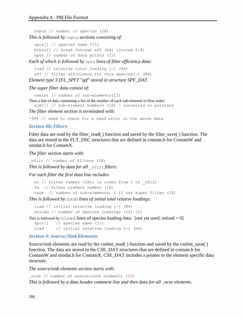
Appendix A - PRJ File Format
286
nspcs // number of species (IX)
This is followed by nspcs sections consisting of:
spcs[] // species name (I1)
bthru[] // break through eff (R4) {Contam 2.4}
npts // number of data points (I2)
Each of which is followed by npts lines of filter efficiency data:
load // relative total loading [-] (R4)
eff // filter efficiency for this species[-] (R4)
Element type 3 [FL_SPF] "spf" stored in structure SPF_DAT.
The super filter data consist of:
nselmt // number of sub-elements(I2)
Then a line of data containing a list of the number of each sub-element in flow order: elmt[] // sub-element numbers (IX) – converted to pointers
The filter element section is terminated with:
-999 // used to check for a read error in the above data
Section 8b: Filters
Filter data are read by the filter_read( ) function and saved by the filter_save( ) function. The
data are stored in the FLT_DSC structures that are defined in contam.h for ContamW and
simdat.h for ContamX.
The filter section starts with:
_nfilt // number of filters (IX)
This is followed by data for all _nfilt filters.
For each filter the first data line includes:
nr // filter number (IX); in order from 1 to _nfilt
fe // filter element number (IX)
nsub // number of sub-elements, 1 if not super filter (IX)
This is followed by nsub lines of initial total relative loadings:
load // initial relative loading [-] (R4)
nsload // number of species loadings (I2) [0]
This is followed by nload lines of species loading data: [not yet used; nsload = 0] spcs[] // species name (I1)
load // initial relative loading [-] (R4)
Section 9: Source/Sink Elements
Source/sink elements are read by the cselmt_read( ) function and saved by the cselmt_save( )
function. The data are stored in the CSE_DAT structures that are defined in contam.h for
ContamW and simdat.h for ContamX. CSE_DAT includes a pointer to the element specific data
structure.
The source/sink elements section starts with:
_ncse // number of source/sink elements (IX)
This is followed by a data header comment line and then data for all _ncse elements.
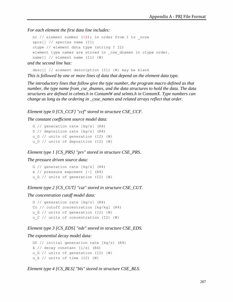
Appendix A - PRJ File Format
287
For each element the first data line includes:
nr // element number (IX); in order from 1 to _ncse
spcs[] // species name (I1)
ctype // element data type (string ? I2)
element type names are stored in _cse_dnames in ctype order.
name[] // element name (I1) {W}
and the second line has:
desc[] // element description (I1) {W} may be blank
This is followed by one or more lines of data that depend on the element data type.
The introductory lines that follow give the type number, the program macro defined as that
number, the type name from_cse_dnames, and the data structures to hold the data. The data
structures are defined in celmts.h in ContamW and selmts.h in ContamX. Type numbers can
change as long as the ordering in _csse_names and related arrays reflect that order.
Element type 0 [CS_CCF] "ccf" stored in structure CSE_CCF.
The constant coefficient source model data:
G // generation rate [kg/s] (R4)
D // deposition rate [kg/s] (R4)
u_G // units of generation (I2) {W}
u_D // units of deposition (I2) {W}
Element type 1 [CS_PRS] "prs" stored in structure CSE_PRS.
The pressure driven source data:
G // generation rate [kg/s] (R4)
x // pressure exponent [-] (R4)
u_G // units of generation (I2) {W}
Element type 2 [CS_CUT] "cut" stored in structure CSE_CUT.
The concentration cutoff model data:
G // generation rate [kg/s] (R4)
Co // cutoff concentration [kg/kg] (R4)
u_G // units of generation (I2) {W}
u_C // units of concentration (I2) {W}
Element type 3 [CS_EDS] "eds" stored in structure CSE_EDS.
The exponential decay model data:
G0 // initial generation rate [kg/s] (R4)
k // decay constant [1/s] (R4)
u_G // units of generation (I2) {W}
u_k // units of time (I2) {W}
Element type 4 [CS_BLS] "bls" stored in structure CSE_BLS.

Appendix A - PRJ File Format
288
The boundary layer diffusion model data:
hm // average film mass transfer coefficient [m/s] (R4)
rho // film density of air [kg/m^3] (R4)
Kp // partition coefficient (R4)
M // adsorbent mass/unit area [kg/m^2] (R4)
u_h // units of hm (I2) {W}
u_r // units of rho (I2) {W}
u_M // units of M (I2) {W}
Element type 5 [CS_BRS] "brs" stored in structure CSE_BRS.
The burst source data:
M // mass added to zone in one time step [kg] (R4)
u_M // units of mass (I2) {W}
Element type 6 [CS_DVS] "dvs" stored in structure CSE_DVS.
The deposition velocity sink model data:
dV // deposition velocity [m/s] (R4)
dA // deposition area [m^2] (R4)
u_V // units of velocity (I2) {W}
u_A // units of area (I2) {W}
Element type 7 [CS_DRS] "drs" stored in structure CSE_DRS.
The deposition rate sink model data:
kd // deposition rate [1/s] (R4)
u_k // units of deposition rate (I2) {W}
Element type 8 [CS_DVR] "dvr" stored in structure CSE_DVR. {CONTAM 3.0}
The deposition velocity resuspension source/sink model data:
dV // deposition velocity [m/s] (R4)
R // resuspension rate [1/s] (R4)
dA // deposition surface area [m2] (R4)
rA // resuspension surface area [m2] (R4)
u_V // units of deposition velocity (I2) {W}
u_R // units of resuspension rate (I2) {W}
u_dA // units of deposition areaa (I2) {W}
u_dR // units of resuspension area (I2) {W}
Element type 11 [CS_PLM] "plm" stored in structure CSE_PLM. {CONTAM 2.4b}
The NRCC power law model data:
a // coefficient(R4) [kg/s]
b // exponent (R4)
tp // PL model time [s] (R4)
u_a // units of initial emission factor (I2) {W}
u_tp // units of PL model time (I2) {W}
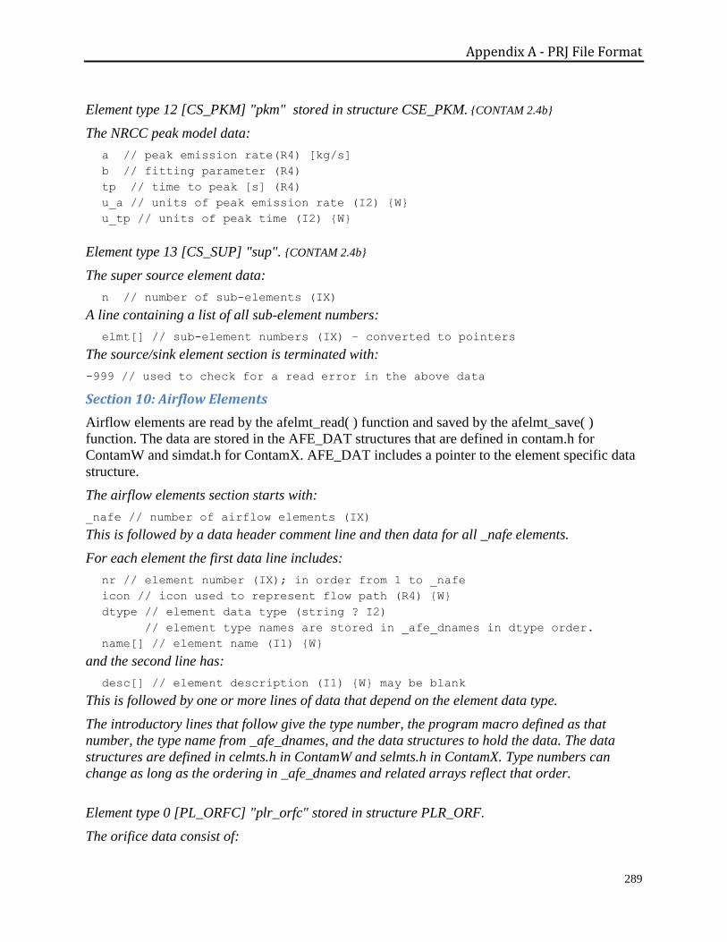
Appendix A - PRJ File Format
289
Element type 12 [CS_PKM] "pkm" stored in structure CSE_PKM. {CONTAM 2.4b}
The NRCC peak model data:
a // peak emission rate(R4) [kg/s]
b // fitting parameter (R4)
tp // time to peak [s] (R4)
u_a // units of peak emission rate (I2) {W}
u_tp // units of peak time (I2) {W}
Element type 13 [CS_SUP] "sup". {CONTAM 2.4b}
The super source element data:
n // number of sub-elements (IX)
A line containing a list of all sub-element numbers:
elmt[] // sub-element numbers (IX) – converted to pointers
The source/sink element section is terminated with:
-999 // used to check for a read error in the above data
Section 10: Airflow Elements
Airflow elements are read by the afelmt_read( ) function and saved by the afelmt_save( )
function. The data are stored in the AFE_DAT structures that are defined in contam.h for
ContamW and simdat.h for ContamX. AFE_DAT includes a pointer to the element specific data
structure.
The airflow elements section starts with:
_nafe // number of airflow elements (IX)
This is followed by a data header comment line and then data for all _nafe elements.
For each element the first data line includes:
nr // element number (IX); in order from 1 to _nafe
icon // icon used to represent flow path (R4) {W}
dtype // element data type (string ? I2)
// element type names are stored in _afe_dnames in dtype order.
name[] // element name (I1) {W}
and the second line has:
desc[] // element description (I1) {W} may be blank
This is followed by one or more lines of data that depend on the element data type.
The introductory lines that follow give the type number, the program macro defined as that
number, the type name from _afe_dnames, and the data structures to hold the data. The data
structures are defined in celmts.h in ContamW and selmts.h in ContamX. Type numbers can
change as long as the ordering in _afe_dnames and related arrays reflect that order.
Element type 0 [PL_ORFC] "plr_orfc" stored in structure PLR_ORF.
The orifice data consist of:
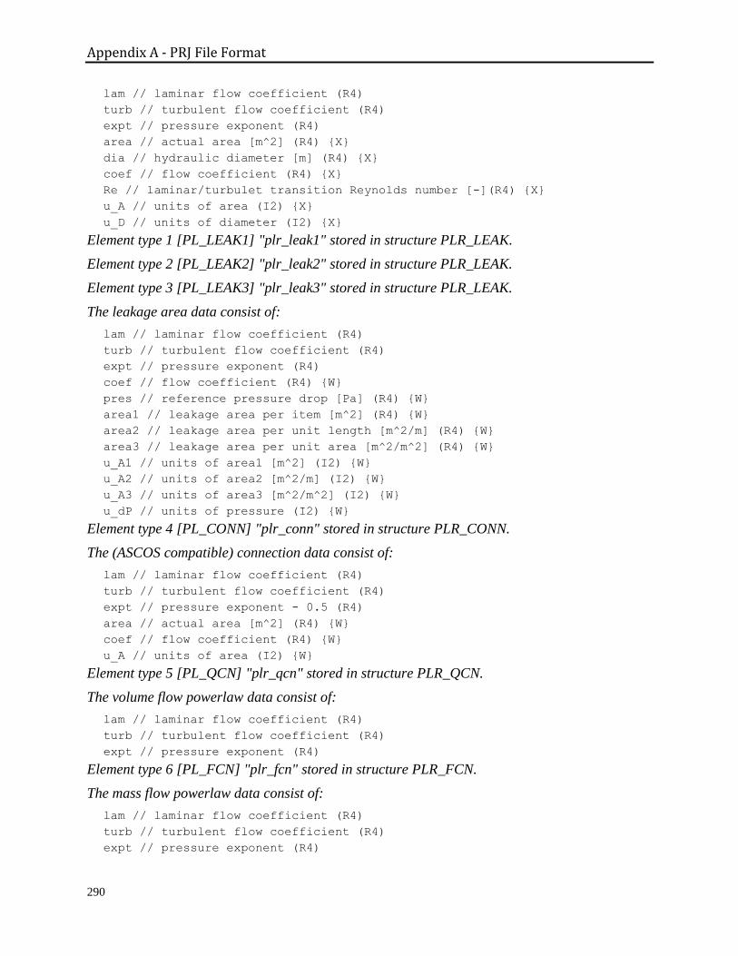
Appendix A - PRJ File Format
290
lam // laminar flow coefficient (R4)
turb // turbulent flow coefficient (R4)
expt // pressure exponent (R4)
area // actual area [m^2] (R4) {X}
dia // hydraulic diameter [m] (R4) {X}
coef // flow coefficient (R4) {X}
Re // laminar/turbulet transition Reynolds number [-](R4) {X}
u_A // units of area (I2) {X}
u_D // units of diameter (I2) {X}
Element type 1 [PL_LEAK1] "plr_leak1" stored in structure PLR_LEAK.
Element type 2 [PL_LEAK2] "plr_leak2" stored in structure PLR_LEAK.
Element type 3 [PL_LEAK3] "plr_leak3" stored in structure PLR_LEAK.
The leakage area data consist of:
lam // laminar flow coefficient (R4)
turb // turbulent flow coefficient (R4)
expt // pressure exponent (R4)
coef // flow coefficient (R4) {W}
pres // reference pressure drop [Pa] (R4) {W}
area1 // leakage area per item [m^2] (R4) {W}
area2 // leakage area per unit length [m^2/m] (R4) {W}
area3 // leakage area per unit area [m^2/m^2] (R4) {W}
u_A1 // units of area1 [m^2] (I2) {W}
u_A2 // units of area2 [m^2/m] (I2) {W}
u_A3 // units of area3 [m^2/m^2] (I2) {W}
u_dP // units of pressure (I2) {W}
Element type 4 [PL_CONN] "plr_conn" stored in structure PLR_CONN.
The (ASCOS compatible) connection data consist of:
lam // laminar flow coefficient (R4)
turb // turbulent flow coefficient (R4)
expt // pressure exponent - 0.5 (R4)
area // actual area [m^2] (R4) {W}
coef // flow coefficient (R4) {W}
u_A // units of area (I2) {W}
Element type 5 [PL_QCN] "plr_qcn" stored in structure PLR_QCN.
The volume flow powerlaw data consist of:
lam // laminar flow coefficient (R4)
turb // turbulent flow coefficient (R4)
expt // pressure exponent (R4)
Element type 6 [PL_FCN] "plr_fcn" stored in structure PLR_FCN.
The mass flow powerlaw data consist of:
lam // laminar flow coefficient (R4)
turb // turbulent flow coefficient (R4)
expt // pressure exponent (R4)
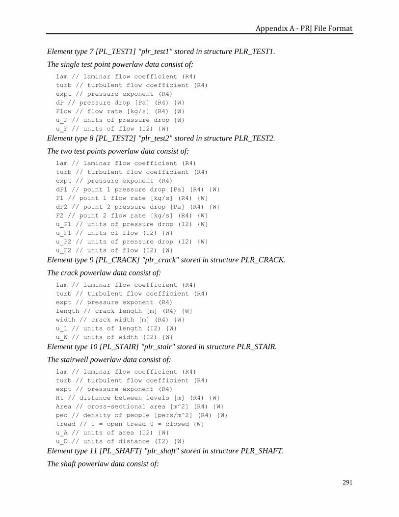
Appendix A - PRJ File Format
291
Element type 7 [PL_TEST1] "plr_test1" stored in structure PLR_TEST1.
The single test point powerlaw data consist of:
lam // laminar flow coefficient (R4)
turb // turbulent flow coefficient (R4)
expt // pressure exponent (R4)
dP // pressure drop [Pa] (R4) {W}
Flow // flow rate [kg/s] (R4) {W}
u_P // units of pressure drop {W}
u_F // units of flow (I2) {W}
Element type 8 [PL_TEST2] "plr_test2" stored in structure PLR_TEST2.
The two test points powerlaw data consist of:
lam // laminar flow coefficient (R4)
turb // turbulent flow coefficient (R4)
expt // pressure exponent (R4)
dP1 // point 1 pressure drop [Pa] (R4) {W}
F1 // point 1 flow rate [kg/s] (R4) {W}
dP2 // point 2 pressure drop [Pa] (R4) {W}
F2 // point 2 flow rate [kg/s] (R4) {W}
u_P1 // units of pressure drop (I2) {W}
u_F1 // units of flow (I2) {W}
u_P2 // units of pressure drop (I2) {W}
u_F2 // units of flow (I2) {W}
Element type 9 [PL_CRACK] "plr_crack" stored in structure PLR_CRACK.
The crack powerlaw data consist of:
lam // laminar flow coefficient (R4)
turb // turbulent flow coefficient (R4)
expt // pressure exponent (R4)
length // crack length [m] (R4) {W}
width // crack width [m] (R4) {W}
u_L // units of length (I2) {W}
u_W // units of width (I2) {W}
Element type 10 [PL_STAIR] "plr_stair" stored in structure PLR_STAIR.
The stairwell powerlaw data consist of:
lam // laminar flow coefficient (R4)
turb // turbulent flow coefficient (R4)
expt // pressure exponent (R4)
Ht // distance between levels [m] (R4) {W}
Area // cross-sectional area [m^2] (R4) {W}
peo // density of people [pers/m^2] (R4) {W}
tread // 1 = open tread 0 = closed {W}
u_A // units of area (I2) {W}
u_D // units of distance (I2) {W}
Element type 11 [PL_SHAFT] "plr_shaft" stored in structure PLR_SHAFT.
The shaft powerlaw data consist of:

Appendix A - PRJ File Format
292
lam // laminar flow coefficient (R4)
turb // turbulent flow coefficient (R4)
expt // pressure exponent (R4)
Ht // distance between levels [m] (R4) {W}
area // cross-sectional area [m^2] (R4) {W}
perim // perimeter [m] (R4) {W}
rough // roughness [m] (R4) {W}
u_A // units of area (I2) {W}
u_D // units of distance (I2) {W}
u_P // units of perimeter (I2) {W}
u_R // units of roughness (I2) {W}
Element type 12 [PL_BDQ] "plr_bdq" stored in structure PLR_BDQ.
The volume flow powerlaw backdraft damper data consist of:
lam // laminar flow coefficient {R4}
Cp // turbulent flow coefficient ( dP > 0 ) {R4}
xp // pressure exponent ( dP > 0 ) {R4}
Cn // turbulent flow coefficient ( dP < 0 ) {R4}
xn // pressure exponent ( dP < 0 ) {R4}
Element type 13 [PL_BDF] "plr_bdf" stored in structure PLR_BDF.
The mass flow powerlaw backdraft damper data consist of:
lam // laminar flow coefficient {R4}
Cp // turbulent flow coefficient ( dP > 0 ) {R4}
xp // pressure exponent ( dP > 0 ) {R4}
Cn // turbulent flow coefficient ( dP < 0 ) {R4}
xn // pressure exponent ( dP < 0 ) {R4}
Element type 14 [QFR_QAB] "qfr_qab" stored in structure QFR_QAB.
The volume flow quadratic data consist of:
a // dP = a*Q + b*Q*Q {R4}
b // {R4}
Element type 15 [QFR_QAF] "qfr_fab" stored in structure QFR_FAB.
The mass flow quadratic data consist of:
a // dP = a*F + b*F*F {R4}
b // {R4}
Element type 16 [QFR_CRACK] "qfr_crack" stored in structure QFR_CRACK.
The crack mass flow quadratic data consist of:
a // dP = a*F + b*F*F {R4}
b // {R4}
length // crack length [m] {R4}
width // crack width [m] {R4}
depth // crack depth [m] {R4}
nB // number of bends
u_L // units of length
u_W // units of width
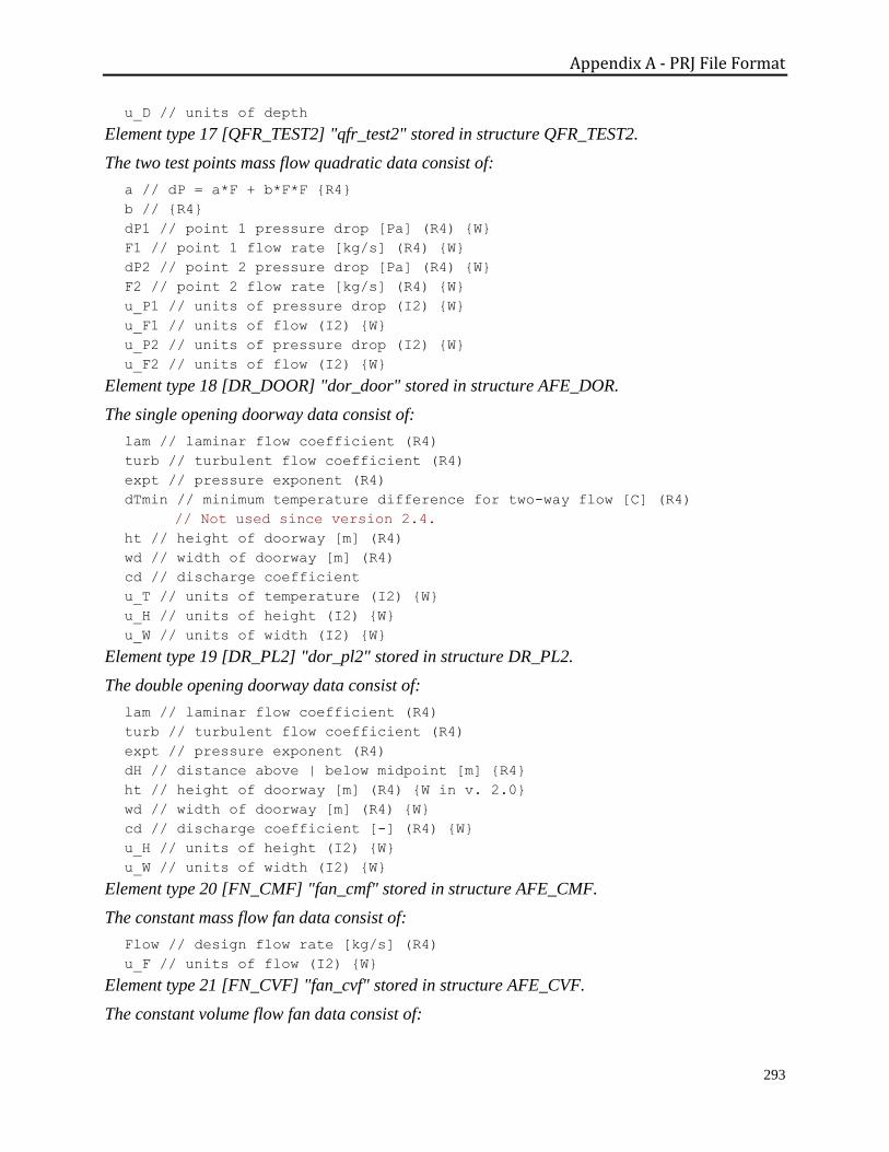
Appendix A - PRJ File Format
293
u_D // units of depth
Element type 17 [QFR_TEST2] "qfr_test2" stored in structure QFR_TEST2.
The two test points mass flow quadratic data consist of:
a // dP = a*F + b*F*F {R4}
b // {R4}
dP1 // point 1 pressure drop [Pa] (R4) {W}
F1 // point 1 flow rate [kg/s] (R4) {W}
dP2 // point 2 pressure drop [Pa] (R4) {W}
F2 // point 2 flow rate [kg/s] (R4) {W}
u_P1 // units of pressure drop (I2) {W}
u_F1 // units of flow (I2) {W}
u_P2 // units of pressure drop (I2) {W}
u_F2 // units of flow (I2) {W}
Element type 18 [DR_DOOR] "dor_door" stored in structure AFE_DOR.
The single opening doorway data consist of:
lam // laminar flow coefficient (R4)
turb // turbulent flow coefficient (R4)
expt // pressure exponent (R4)
dTmin // minimum temperature difference for two-way flow [C] (R4)
// Not used since version 2.4.
ht // height of doorway [m] (R4)
wd // width of doorway [m] (R4)
cd // discharge coefficient
u_T // units of temperature (I2) {W}
u_H // units of height (I2) {W}
u_W // units of width (I2) {W}
Element type 19 [DR_PL2] "dor_pl2" stored in structure DR_PL2.
The double opening doorway data consist of:
lam // laminar flow coefficient (R4)
turb // turbulent flow coefficient (R4)
expt // pressure exponent (R4)
dH // distance above | below midpoint [m] {R4}
ht // height of doorway [m] (R4) {W in v. 2.0}
wd // width of doorway [m] (R4) {W}
cd // discharge coefficient [-] (R4) {W}
u_H // units of height (I2) {W}
u_W // units of width (I2) {W}
Element type 20 [FN_CMF] "fan_cmf" stored in structure AFE_CMF.
The constant mass flow fan data consist of:
Flow // design flow rate [kg/s] (R4)
u_F // units of flow (I2) {W}
Element type 21 [FN_CVF] "fan_cvf" stored in structure AFE_CVF.
The constant volume flow fan data consist of:
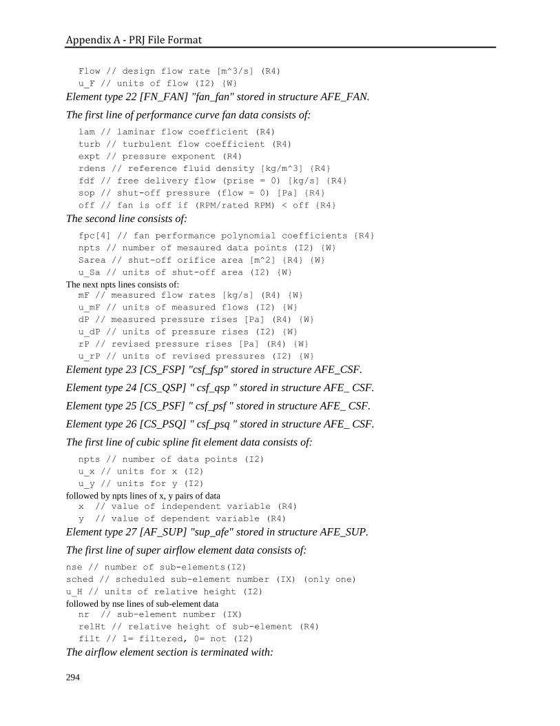
Appendix A - PRJ File Format
294
Flow // design flow rate [m^3/s] (R4)
u_F // units of flow (I2) {W}
Element type 22 [FN_FAN] "fan_fan" stored in structure AFE_FAN.
The first line of performance curve fan data consists of:
lam // laminar flow coefficient (R4)
turb // turbulent flow coefficient (R4)
expt // pressure exponent (R4)
rdens // reference fluid density [kg/m^3] {R4}
fdf // free delivery flow (prise = 0) [kg/s] {R4}
sop // shut-off pressure (flow = 0) [Pa] {R4}
off // fan is off if (RPM/rated RPM) < off {R4}
The second line consists of:
fpc[4] // fan performance polynomial coefficients {R4}
npts // number of mesaured data points (I2) {W}
Sarea // shut-off orifice area [m^2] {R4} {W}
u_Sa // units of shut-off area (I2) {W}
The next npts lines consists of: mF // measured flow rates [kg/s] (R4) {W}
u_mF // units of measured flows (I2) {W}
dP // measured pressure rises [Pa] (R4) {W}
u_dP // units of pressure rises (I2) {W}
rP // revised pressure rises [Pa] (R4) {W}
u_rP // units of revised pressures (I2) {W}
Element type 23 [CS_FSP] "csf_fsp" stored in structure AFE_CSF.
Element type 24 [CS_QSP] " csf_qsp " stored in structure AFE_ CSF.
Element type 25 [CS_PSF] " csf_psf " stored in structure AFE_ CSF.
Element type 26 [CS_PSQ] " csf_psq " stored in structure AFE_ CSF.
The first line of cubic spline fit element data consists of:
npts // number of data points (I2)
u_x // units for x (I2)
u_y // units for y (I2)
followed by npts lines of x, y pairs of data x // value of independent variable (R4)
y // value of dependent variable (R4)
Element type 27 [AF_SUP] "sup_afe" stored in structure AFE_SUP.
The first line of super airflow element data consists of:
nse // number of sub-elements(I2)
sched // scheduled sub-element number (IX) (only one)
u_H // units of relative height (I2)
followed by nse lines of sub-element data nr // sub-element number (IX)
relHt // relative height of sub-element (R4)
filt // 1= filtered, 0= not (I2)
The airflow element section is terminated with:
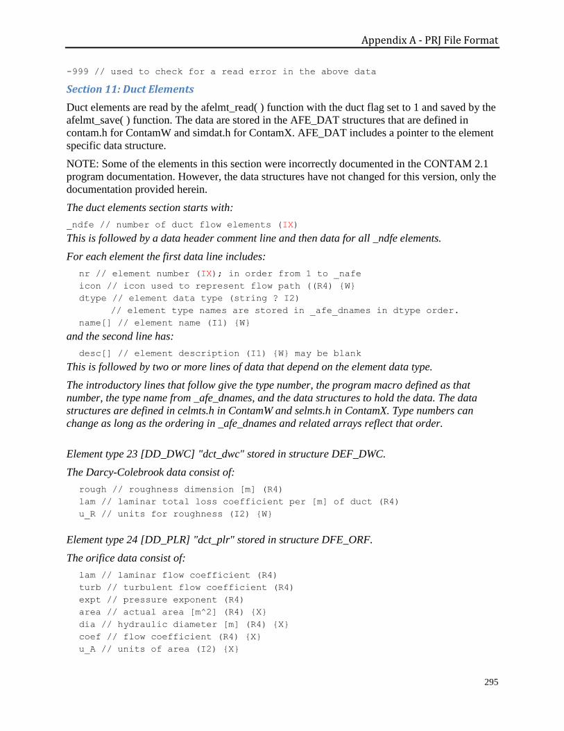
Appendix A - PRJ File Format
295
-999 // used to check for a read error in the above data
Section 11: Duct Elements
Duct elements are read by the afelmt_read( ) function with the duct flag set to 1 and saved by the
afelmt_save( ) function. The data are stored in the AFE_DAT structures that are defined in
contam.h for ContamW and simdat.h for ContamX. AFE_DAT includes a pointer to the element
specific data structure.
NOTE: Some of the elements in this section were incorrectly documented in the CONTAM 2.1
program documentation. However, the data structures have not changed for this version, only the
documentation provided herein.
The duct elements section starts with:
_ndfe // number of duct flow elements (IX)
This is followed by a data header comment line and then data for all _ndfe elements.
For each element the first data line includes:
nr // element number (IX); in order from 1 to _nafe
icon // icon used to represent flow path ((R4) {W}
dtype // element data type (string ? I2)
// element type names are stored in _afe_dnames in dtype order.
name[] // element name (I1) {W}
and the second line has:
desc[] // element description (I1) {W} may be blank
This is followed by two or more lines of data that depend on the element data type.
The introductory lines that follow give the type number, the program macro defined as that
number, the type name from _afe_dnames, and the data structures to hold the data. The data
structures are defined in celmts.h in ContamW and selmts.h in ContamX. Type numbers can
change as long as the ordering in _afe_dnames and related arrays reflect that order.
Element type 23 [DD_DWC] "dct_dwc" stored in structure DEF_DWC.
The Darcy-Colebrook data consist of:
rough // roughness dimension [m] (R4)
lam // laminar total loss coefficient per [m] of duct (R4)
u_R // units for roughness (I2) {W}
Element type 24 [DD_PLR] "dct_plr" stored in structure DFE_ORF.
The orifice data consist of:
lam // laminar flow coefficient (R4)
turb // turbulent flow coefficient (R4)
expt // pressure exponent (R4)
area // actual area [m^2] (R4) {X}
dia // hydraulic diameter [m] (R4) {X}
coef // flow coefficient (R4) {X}
u_A // units of area (I2) {X}
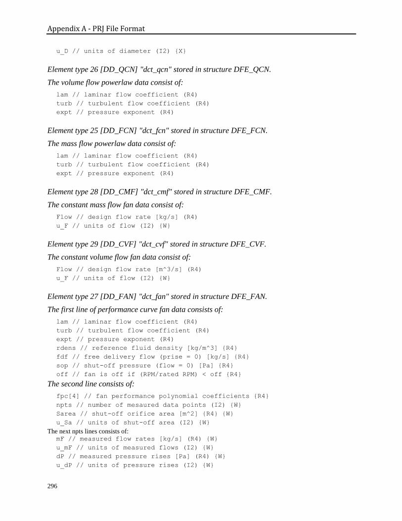
Appendix A - PRJ File Format
296
u_D // units of diameter (I2) {X}
Element type 26 [DD_QCN] "dct_qcn" stored in structure DFE_QCN.
The volume flow powerlaw data consist of:
lam // laminar flow coefficient (R4)
turb // turbulent flow coefficient (R4)
expt // pressure exponent (R4)
Element type 25 [DD_FCN] "dct_fcn" stored in structure DFE_FCN.
The mass flow powerlaw data consist of:
lam // laminar flow coefficient (R4)
turb // turbulent flow coefficient (R4)
expt // pressure exponent (R4)
Element type 28 [DD_CMF] "dct_cmf" stored in structure DFE_CMF.
The constant mass flow fan data consist of:
Flow // design flow rate [kg/s] (R4)
u_F // units of flow (I2) {W}
Element type 29 [DD_CVF] "dct_cvf" stored in structure DFE_CVF.
The constant volume flow fan data consist of:
Flow // design flow rate [m^3/s] (R4)
u_F // units of flow (I2) {W}
Element type 27 [DD_FAN] "dct_fan" stored in structure DFE_FAN.
The first line of performance curve fan data consists of:
lam // laminar flow coefficient (R4)
turb // turbulent flow coefficient (R4)
expt // pressure exponent (R4)
rdens // reference fluid density [kg/m^3] {R4}
fdf // free delivery flow (prise = 0) [kg/s] {R4}
sop // shut-off pressure (flow = 0) [Pa] {R4}
off // fan is off if (RPM/rated RPM) < off {R4}
The second line consists of:
fpc[4] // fan performance polynomial coefficients {R4}
npts // number of mesaured data points (I2) {W}
Sarea // shut-off orifice area [m^2] {R4} {W}
u_Sa // units of shut-off area (I2) {W}
The next npts lines consists of: mF // measured flow rates [kg/s] (R4) {W}
u_mF // units of measured flows (I2) {W}
dP // measured pressure rises [Pa] (R4) {W}
u_dP // units of pressure rises (I2) {W}
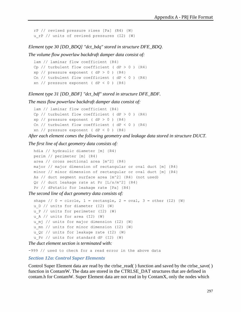
Appendix A - PRJ File Format
297
rP // revised pressure rises [Pa] (R4) {W}
u_rP // units of revised pressures (I2) {W}
Element type 30 [DD_BDQ] "dct_bdq" stored in structure DFE_BDQ.
The volume flow powerlaw backdraft damper data consist of:
lam // laminar flow coefficient {R4}
Cp // turbulent flow coefficient ( dP > 0 ) {R4}
xp // pressure exponent ( dP > 0 ) {R4}
Cn // turbulent flow coefficient ( dP < 0 ) {R4}
xn // pressure exponent ( dP < 0 ) {R4}
Element type 31 [DD_BDF] "dct_bdf" stored in structure DFE_BDF.
The mass flow powerlaw backdraft damper data consist of:
lam // laminar flow coefficient {R4}
Cp // turbulent flow coefficient ( dP > 0 ) {R4}
xp // pressure exponent ( dP > 0 ) {R4}
Cn // turbulent flow coefficient ( dP < 0 ) {R4}
xn // pressure exponent ( dP < 0 ) {R4}
After each element comes the following geometry and leakage data stored in structure DUCT.
The first line of duct geometry data consists of:
hdia // hydraulic diameter [m] {R4}
perim // perimeter [m] {R4}
area // cross sectional area [m^2] {R4}
major // major dimension of rectangular or oval duct [m] {R4}
minor // minor dimension of rectangular or oval duct [m] {R4}
As // duct segment surface area [m^2] {R4} (not used)
Qr // duct leakage rate at Pr [L/s/m^2] {R4}
Pr // dPstatic for leakage rate [Pa] {R4}
The second line of duct geometry data consists of:
shape // 0 = circle, 1 = rectangle, 2 = oval, 3 = other (I2) {W}
u_D // units for diameter (I2) {W}
u_P // units for perimeter (I2) {W}
u_A // units for area (I2) {W}
u_mj // units for major dimension (I2) {W}
u_mn // units for minor dimension (I2) {W}
u_Qr // units for leakage rate (I2) {W}
u_Pr // units for standard dP (I2) {W}
The duct element section is terminated with:
-999 // used to check for a read error in the above data
Section 12a: Control Super Elements
Control Super Element data are read by the ctrlse_read( ) function and saved by the ctrlse_save( )
function in ContamW. The data are stored in the CTRLSE_DAT structures that are defined in
contam.h for ContamW. Super Element data are not read in by ContamX, only the nodes which
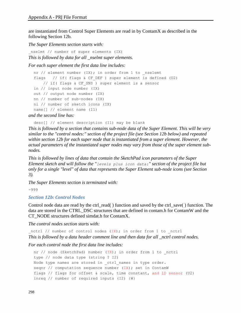
Appendix A - PRJ File Format
298
are instantiated from Control Super Elements are read in by ContamX as described in the
following Section 12b.
The Super Elements section starts with:
_nselmt // number of super elements (IX)
This is followed by data for all _nselmt super elements.
For each super element the first data line includes:
nr // element number (IX); in order from 1 to _nselemt
flags // if( flags & CF_DEF ) super element is defined (U2)
// if( flags & CF_SNS ) super element is a sensor
in // input node number (IX)
out // output node number (IX)
nn // number of sub-nodes (IX)
ni // number of sketch icons (IX)
name[] // element name (I1)
and the second line has:
desc[] // element description (I1) may be blank
This is followed by a section that contains sub-node data of the Super Element. This will be very
similar to the "control nodes:" section of the project file (see Section 12b below) and repeated
within section 12b for each super node that is instantiated from a super element. However, the
actual parameters of the instantiated super nodes may vary from those of the super element sub-
nodes.
This is followed by lines of data that contain the SketchPad icon parameters of the Super
Element sketch and will follow the "levels plus icon data:" section of the project file but
only for a single "level" of data that represents the Super Element sub-node icons (see Section
3).
The Super Elements section is terminated with:
-999
Section 12b: Control Nodes
Control node data are read by the ctrl_read( ) function and saved by the ctrl_save( ) function. The
data are stored in the CTRL_DSC structures that are defined in contam.h for ContamW and the
CT_NODE structures defined simdat.h for ContamX.
The control nodes section starts with:
_nctrl // number of control nodes (IX); in order from 1 to _nctrl
This is followed by a data header comment line and then data for all _nctrl control nodes.
For each control node the first data line includes:
nr // node (SketchPad) number (IX); in order from 1 to _nctrl
type // node data type (string ? I2)
Node type names are stored in _ctrl_names in type order.
seqnr // computation sequence number (IX); set in ContamW
flags // flags for offset & scale, time constant, and 1D sensor (U2)
inreq // number of required inputs (I2) {W}

Appendix A - PRJ File Format
299
n1 // SketchPad number of input node #1 (IX)
n2 // SketchPad number of input node #2 (IX)
name[] // element name (I1) {W}
and the second line has:
desc[] // control node description (I1) {W} may be blank
This may be followed by one more line of data that depends on the node type.
Node type 0 [CT_SNS] "sns" stored in structure SENSOR {W} or SNSDAT {X}.
offset // offset value (R4)
scale // scale value (R4)
tau // time constant (R4)
oldsig // signal at last time step - for restart (R4)
source // index of source (source not defined at read time) (IX)
type // type of source: 1=zone, 2=path, 3=junction, 4=duct,
// 5=exp, 6=term (I2)
measure // 0=contaminant, 1=temperature, 2=flow rate, 3=dP,
// 4=Pgage, 5=zone occupancy (I2)
X // X-coordinate of sensor [m] (R4)
Y // Y-coordinate of sensor [m] (R4)
relHt // relative height of sensor [m] (R4)
units[] // units of coordinates {W} (I1)
species[] // species name [I1]; convert to pointer
Node type 1 [CT_SCH] "sch" stored in structure SCHDAT.
ps // week schedule index (I2); converted to pointer
Node type 2 [CT_SET] "set" stored in structure SETDAT.
value // constant value (R4)
Node type 3 [CT_CVF] "cvf" stored in structure CDVDAT. {Contam 2.1}
name[] // name of the value read from the Continuous Values file (I1)
Node type 4 [CT_DVF] "dvf" stored in structure CDVDAT. {Contam 2.1}
name[] // name of the value read from the Discrete Values file (I1)
Node type 5 [CT_LOG] "log" stored in structure LOGDAT.
offset // offset value (R4)
scale // scale value (R4)
udef // true if using default units (I2) {W}
header[] // header string (I1)
units[] // units string (I1)
Node type 6 [CT_PAS] "pas" has no additional data.
Node type 7 [CT_MOD] "mod" stored in structure MOD.
offset // offset value (R4)
scale // scale value (R4)
Node type 8 [CT_HYS] "hys" stored in structure HYSDAT.
slack; // hysteresis parameter (R4)
slope // 1.0 / (1.0 - slack) (R4)
oldsig // prior output signal (R4)

Appendix A - PRJ File Format
300
Node type 9 [CT_ABS] "abs" has no additional data.
Node type 10 [CT_BIN] "bin" has no additional data.
Node type 11 [CT_DLS] "dls" stored in structure CDVDAT. {Contam 2.1}
dsincr // day schedule number for increasing signal (I2)
dsdecr // day schedule number for decreasing signal (I2)
Node type 12 [CT_DLX] "dlx" stored in structure CDVDAT. {Contam 2.1}
tauincr // time constant for increasing signal [s] (I4)
taudecr // time constant for decreasing signal [s] (I4)
Node type 13 [CT_INT] "int" has no additional data.
Node type 14 [CT_RAV] "rav" stored in structure CDVDAT. {Contam 2.1}
tspan // time span for the running average [s] (I4)
Node type 15 [CT_INV] "inv" has no additional data.
Node type 16 [CT_AND] "and" has no additional data.
Node type 17 [CT_OR] "od" has no additional data.
Node type 18 [CT_XOR] "xor" has no additional data.
Node type 19 [CT_ADD] "add" has no additional data.
Node type 20 [CT_SUB] "sub" has no additional data.
Node type 21 [CT_MUL] "mul" has no additional data.
Node type 22 [CT_DIV] "div" has no additional data.
Node type 23 [CT_SUM] "sum" stored in structure SUMAVG.
Node type 24 [CT_AVG] "avg" stored in structure SUMAVG.
Node type 25 [CT_MAX] "max" stored in structure SUMAVG.
Node type 26 [CT_MIN] "min" stored in structure SUMAVG.
npcs // number of controls to be processed (IX)
pc[npcs] // indices of npcs control nodes (IX)
Node type 27 [CT_LLS] "lls" has no additional data.
Node type 28 [CT_ULS] "uls" has no additional data.
Node type 29 [CT_LBS] "lbs" stored in structure BANDAT.
Node type 30 [CT_UBS] "ubs" stored in structure BANDAT.
band // width of band (R4)
Node type 31 [CT_LLC] "llc" has no additional data.
Node type 32 [CT_ULC] "ulc" has no additional data.
Node type 33 [CT_PC1] "pc1" stored in structure PCDAT.
kp // proportional gain factor (R4)
Node type 34 [CT_PI1] "pi1" stored in structure PICDAT.
kp // proportional gain factor (R4)

Appendix A - PRJ File Format
301
ki // integral gain factor (R4)
oldsig // prior output signal - for restart (R4)
olderr // prior error value - for restart (R4)
Node type 35 [CT_SUP] "sup" stored in structure SUPDAT.
def // 0:super element undefined 1:defined (I2)
se // super element number (IX)
in // input sub-node number (IX)
out // output sub-node number (IX)
Node type 36 [CT_SEN] this is only a placeholder value for use with the type dialog.
Node type 37 [CT_SPH] "sph" has no additional data.
The control nodes section is terminated with:
-999 // used to check for a read error in the above data
Section 13: Simple Air Handling System (AHS)
AHS data are read by the system_read( ) function and saved by the system_save( ) function. The
data are stored in the AHS_DSC structures that are defined in contam.h for ContamW and
simdat.h for ContamX.
The AHS section starts with:
_nahs // number of AHS (IX)
This is followed by a data header comment line and then data for all _nahs systems.
For each AHS the first data line includes:
nr // AHS number (IX); in order from 1 to _nahs
zone_r // return zone number (IX)
zone_s // supply zone number (IX)
path_r // recircultaion air path number (IX)
path_s // outdoor air path number (IX)
path_x // exhaust path number (IX)
and the second line has:
desc[] // AHS description (I1) {W} may be blank
The AHS section is terminated with:
-999 // used to check for a read error in the above data
Section 14: Zones
Zone data are read by the zone_read( ) function and saved by the zone_save( ) function. The data
are stored in the ZONE_DSC structures that are defined in contam.h for ContamW and simdat.h
for ContamX.
The zone section starts with:
_nzone // number of zones (IX)
This is followed by a data header comment line and then data for all _nzone zones.
For each zone the data line includes:
nr // zone number (IX); in order from 1 to _nzone
flags // zone flags – bits defined in contam.h (U2)
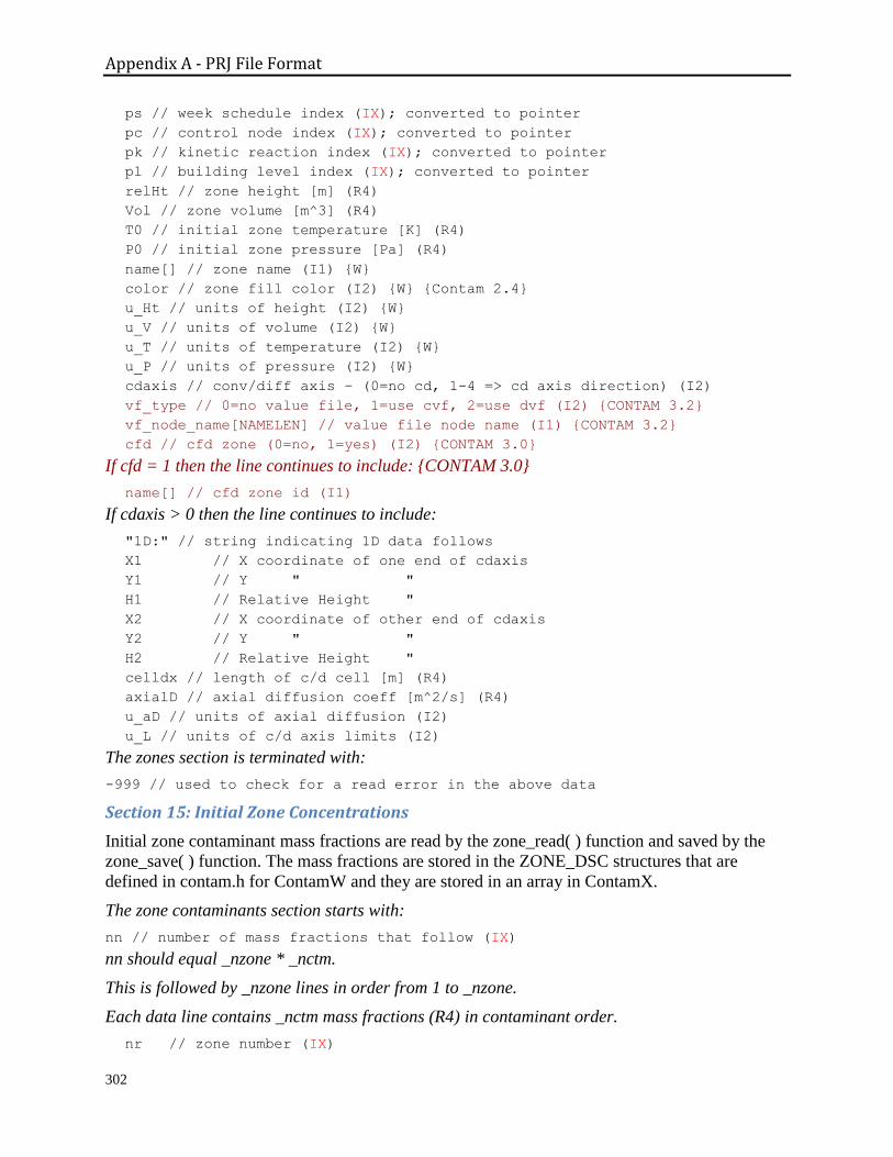
Appendix A - PRJ File Format
302
ps // week schedule index (IX); converted to pointer
pc // control node index (IX); converted to pointer
pk // kinetic reaction index (IX); converted to pointer
pl // building level index (IX); converted to pointer
relHt // zone height [m] (R4)
Vol // zone volume [m^3] (R4)
T0 // initial zone temperature [K] (R4)
P0 // initial zone pressure [Pa] (R4)
name[] // zone name (I1) {W}
color // zone fill color (I2) {W} {Contam 2.4}
u_Ht // units of height (I2) {W}
u_V // units of volume (I2) {W}
u_T // units of temperature (I2) {W}
u_P // units of pressure (I2) {W}
cdaxis // conv/diff axis – (0=no cd, 1-4 => cd axis direction) (I2)
vf_type // 0=no value file, 1=use cvf, 2=use dvf (I2) {CONTAM 3.2}
vf_node_name[NAMELEN] // value file node name (I1) {CONTAM 3.2}
cfd // cfd zone (0=no, 1=yes) (I2) {CONTAM 3.0}
If cfd = 1 then the line continues to include: {CONTAM 3.0}
name[] // cfd zone id (I1)
If cdaxis > 0 then the line continues to include:
"1D:" // string indicating 1D data follows
X1 // X coordinate of one end of cdaxis
Y1 // Y " "
H1 // Relative Height "
X2 // X coordinate of other end of cdaxis
Y2 // Y " "
H2 // Relative Height "
celldx // length of c/d cell [m] (R4)
axialD // axial diffusion coeff [m^2/s] (R4)
u_aD // units of axial diffusion (I2)
u_L // units of c/d axis limits (I2)
The zones section is terminated with:
-999 // used to check for a read error in the above data
Section 15: Initial Zone Concentrations
Initial zone contaminant mass fractions are read by the zone_read( ) function and saved by the
zone_save( ) function. The mass fractions are stored in the ZONE_DSC structures that are
defined in contam.h for ContamW and they are stored in an array in ContamX.
The zone contaminants section starts with:
nn // number of mass fractions that follow (IX)
nn should equal _nzone * _nctm.
This is followed by _nzone lines in order from 1 to _nzone.
Each data line contains _nctm mass fractions (R4) in contaminant order.
nr // zone number (IX)

Appendix A - PRJ File Format
303
CC0[i][1] // initial mass fraction (R4) of zone i, contaminant 1
...
CC0[i][_nctm] // initial mass fraction (R4) of zone i, contaminant _nctm
The initial zone concentrations section is terminated with:
-999 // used to check for a read error in the above data
Section 16: Airflow Paths
Path data are read by the path_read( ) function and saved by the path_save( ) function. The data
are stored in the PATH_DSC structures that are defined in contam.h for ContamW and simdat.h
for ContamX.
The path section starts with:
_npath // number of paths (IX)
This is followed by a data header comment line and then data for all _npath paths.
For each path the data line includes:
nr // path number (IX); in order from 1 to _npath
flags // airflow path flag values (I2)
pzn // zone N index (IX); converted to pointer
pzm // zone M index (IX); converted to pointer
pe // flow element index (IX); converted to pointer
pf // filter index (IX); converted to pointer
pw // wind coefficients index (IX); converted to pointer
pa // AHS index (IX); converted to pointer
ps // schedule index (IX); converted to pointer
pc // control node index (IX); converted to pointer
pld // level index (IX); converted to pointer
X // X-coordinate of envelope path [m] (R4) {Contam 2.1}
Y // Y-coordinate of envelope path [m] (R4) {Contam 2.1}
relHt // height relative to current level [m] (R4)
mult // element multiplier (R4)
wPset // constant wind pressure [Pa] (pw==NULL) (R4)
wPmod // wind speed(?) modifier (pw!=NULL) (R4)
wazm // wall azimuth angle (pw!=NULL) (R4)
Fahs // AHS path flow rate [kg/s] (pw==NULL) (R4)
Xmax // flow or pressure limit - maximum (R4) {W}
Xmin // flow or pressure limit - minimum (R4) {W}
icon // icon used to represent flow path (U1) {W}
dir // positive flow direction on sketchpad (U1) {W}
u_Ht // units of height (I2) {W}
u_XY // units of X and Y (I2) {W}
u_dP // units of pressure difference (I2) {W}
u_F // units of flow (I2) {W}
vf_type // 0=no value file, 1=use cvf, 2=use dvf (I2) {CONTAM 3.2}
vf_node_name[NAMELEN] // value file node name (I1) {CONTAM 3.2}
cfd // cfd path (0=no, 1=yes) (I2) {CONTAM 3.0}
If cfd = 1 then the line continues to include: {CONTAM 3.0}
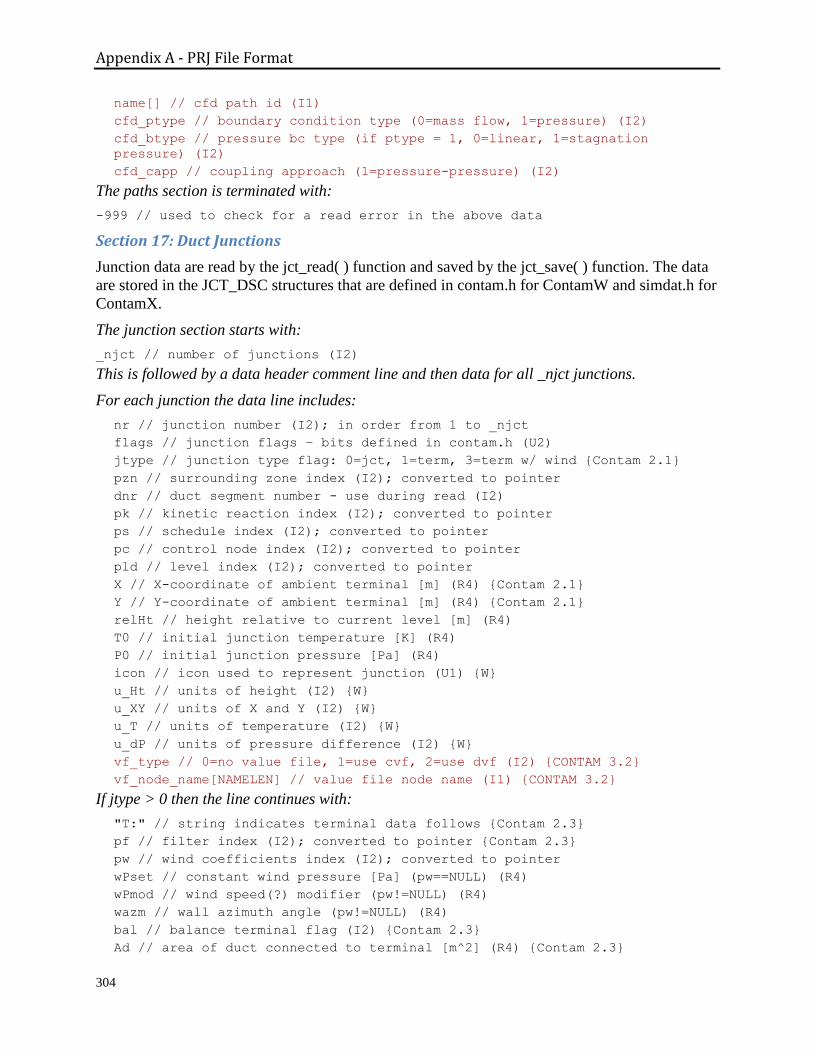
Appendix A - PRJ File Format
304
name[] // cfd path id (I1)
cfd_ptype // boundary condition type (0=mass flow, 1=pressure) (I2)
cfd_btype // pressure bc type (if ptype = 1, 0=linear, 1=stagnation
pressure) (I2)
cfd_capp // coupling approach (1=pressure-pressure) (I2)
The paths section is terminated with:
-999 // used to check for a read error in the above data
Section 17: Duct Junctions
Junction data are read by the jct_read( ) function and saved by the jct_save( ) function. The data
are stored in the JCT_DSC structures that are defined in contam.h for ContamW and simdat.h for
ContamX.
The junction section starts with:
_njct // number of junctions (I2)
This is followed by a data header comment line and then data for all _njct junctions.
For each junction the data line includes:
nr // junction number (I2); in order from 1 to _njct
flags // junction flags – bits defined in contam.h (U2)
jtype // junction type flag: 0=jct, 1=term, 3=term w/ wind {Contam 2.1}
pzn // surrounding zone index (I2); converted to pointer
dnr // duct segment number - use during read (I2)
pk // kinetic reaction index (I2); converted to pointer
ps // schedule index (I2); converted to pointer
pc // control node index (I2); converted to pointer
pld // level index (I2); converted to pointer
X // X-coordinate of ambient terminal [m] (R4) {Contam 2.1}
Y // Y-coordinate of ambient terminal [m] (R4) {Contam 2.1}
relHt // height relative to current level [m] (R4)
T0 // initial junction temperature [K] (R4)
P0 // initial junction pressure [Pa] (R4)
icon // icon used to represent junction (U1) {W}
u_Ht // units of height (I2) {W}
u_XY // units of X and Y (I2) {W}
u_T // units of temperature (I2) {W}
u_dP // units of pressure difference (I2) {W}
vf_type // 0=no value file, 1=use cvf, 2=use dvf (I2) {CONTAM 3.2}
vf_node_name[NAMELEN] // value file node name (I1) {CONTAM 3.2}
If jtype > 0 then the line continues with:
"T:" // string indicates terminal data follows {Contam 2.3}
pf // filter index (I2); converted to pointer {Contam 2.3}
pw // wind coefficients index (I2); converted to pointer
wPset // constant wind pressure [Pa] (pw==NULL) (R4)
wPmod // wind speed(?) modifier (pw!=NULL) (R4)
wazm // wall azimuth angle (pw!=NULL) (R4)
bal // balance terminal flag (I2) {Contam 2.3}
Ad // area of duct connected to terminal [m^2] (R4) {Contam 2.3}
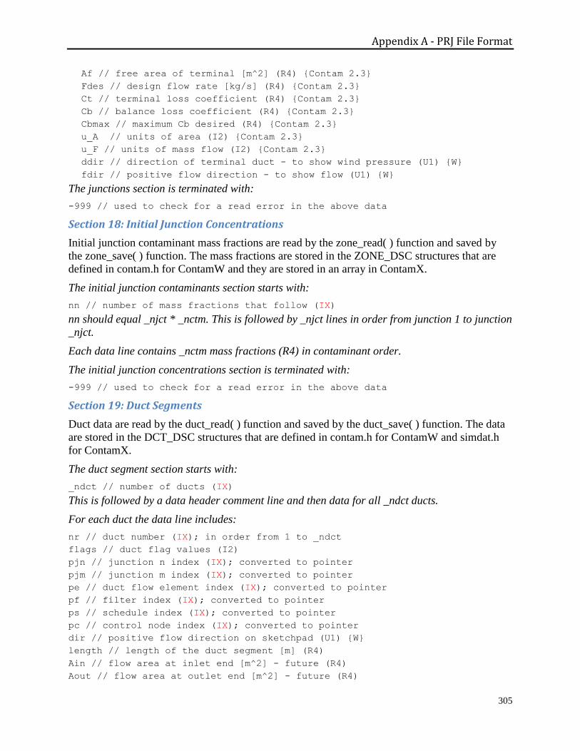
Appendix A - PRJ File Format
305
Af // free area of terminal [m^2] (R4) {Contam 2.3}
Fdes // design flow rate [kg/s] (R4) {Contam 2.3}
Ct // terminal loss coefficient (R4) {Contam 2.3}
Cb // balance loss coefficient (R4) {Contam 2.3}
Cbmax // maximum Cb desired (R4) {Contam 2.3}
u_A // units of area (I2) {Contam 2.3}
u_F // units of mass flow (I2) {Contam 2.3}
ddir // direction of terminal duct - to show wind pressure (U1) {W}
fdir // positive flow direction - to show flow (U1) {W}
The junctions section is terminated with:
-999 // used to check for a read error in the above data
Section 18: Initial Junction Concentrations
Initial junction contaminant mass fractions are read by the zone_read( ) function and saved by
the zone_save( ) function. The mass fractions are stored in the ZONE_DSC structures that are
defined in contam.h for ContamW and they are stored in an array in ContamX.
The initial junction contaminants section starts with:
nn // number of mass fractions that follow (IX)
nn should equal _njct * _nctm. This is followed by _njct lines in order from junction 1 to junction
_njct.
Each data line contains _nctm mass fractions (R4) in contaminant order.
The initial junction concentrations section is terminated with:
-999 // used to check for a read error in the above data
Section 19: Duct Segments
Duct data are read by the duct_read( ) function and saved by the duct_save( ) function. The data
are stored in the DCT_DSC structures that are defined in contam.h for ContamW and simdat.h
for ContamX.
The duct segment section starts with:
_ndct // number of ducts (IX)
This is followed by a data header comment line and then data for all _ndct ducts.
For each duct the data line includes:
nr // duct number (IX); in order from 1 to _ndct
flags // duct flag values (I2)
pjn // junction n index (IX); converted to pointer
pjm // junction m index (IX); converted to pointer
pe // duct flow element index (IX); converted to pointer
pf // filter index (IX); converted to pointer
ps // schedule index (IX); converted to pointer
pc // control node index (IX); converted to pointer
dir // positive flow direction on sketchpad (U1) {W}
length // length of the duct segment [m] (R4)
Ain // flow area at inlet end [m^2] - future (R4)
Aout // flow area at outlet end [m^2] - future (R4)

Appendix A - PRJ File Format
306
sllc // sum of local loss coefficients (R4)
color // icon color (I2) {W} {Contam 2.4}
u_L // units for length (I2) {W}
u_A // units for flow area (I2) {W}
vf_type // 0=no value file, 1=use cvf, 2=use dvf (I2) {CONTAM 3.2}
vf_node_name[NAMELEN] // value file node name (I1) {CONTAM 3.2}
The duct segment section is terminated with:
-999
Section 20: Source/Sinks
Contaminant sources/sinks are read by the css_read( ) function and saved by the css_save( )
function. The data are stored in the CSS_DSC structures that are defined in contam.h for
ContamW and simdat.h for ContamX.
The source/sink section starts with:
_ncss // number of source/sinks (IX)
This is followed by a data header comment line and then data for all _ncss source/sinks.
For each source/sink the data line includes:
nr // source/sink number (IX); in order from 1 to _ncss
pz // zone index (IX); converted to pointer
pe // source/sink element index (IX); converted to pointer
ps // schedule index (IX); converted to pointer
pc // control node index (IX); converted to pointer
mult // multiplier (R4)
CC0 // initial mass fraction (some types) [kg/kg] (R4)
Xmin // minimum x coordinate of source/sink location [m] (R4)
Ymin // minimum y coordinate of source/sink location [m] (R4)
Hmin // minimum z coordinate relative to level [m] (R4)
Xmax // maximum x coordinate of source/sink location [m] (R4)
Ymax // maximum y coordinate of source/sink location [m] (R4)
Hmax // maximum z coordinate relative to level [m] (R4)
u_XYZ // units of location coordinates (I2)
vf_type // 0=no value file, 1=use cvf, 2=use dvf (I2) {CONTAM 3.2}
vf_node_name[NAMELEN] // value file node name (I1) {CONTAM 3.2}
cfd // cfd path (0=no, 1=yes) (I2) {CONTAM 3.0}
If cfd = 1 then the line continues to include: {CONTAM 3.0}
name[] // cfd path id (I1)
The source/sink section is terminated with:
-999 // used to check for a read error in the above data
Section 21: Occupancy Schedules
Occupancy schedules are read by the oschd_read( ) function and saved by the oschd_save( )
function. The data are stored in the OD_SCHD structures that are defined in contam.h for
ContamW and simdat.h for ContamX.
The occupancy schedule section starts with:

Appendix A - PRJ File Format
307
_nosch // number of schedules (IX)
This is followed by a data header comment line and then data for all _nosch schedules.
For each schedule the first data line includes:
nr // schedule number (IX); in order from 1 to _nosch
npts // number of points (I2)
u_XYZ // units of location coordinates (I2)
name[] // schedule name (I1) {W}
and the second line has:
desc[] // schedule description (I1) {W} may be blank
This is followed by npts lines of schedule data:
time // time-of-day [s] (hh:mm:ss converted to I4)
pz // zone index (I2); converted to pointer
X // X-coordinate of occupant [m] (R4)
Y // Y-coordinate of occupant [m] (R4)
relHt // height relative to current level [m] (R4)
The occupancy schedule section is terminated with:
-999 // used to check for a read error in the above data
Section 22: Exposures
Exposure data are read by the pexp_read( ) function and saved by the pexp_save( ) function. The
data are stored in the PEXP_DSC structures that are defined in contam.h for ContamW and
simdat.h for ContamX.
The exposure section starts with:
_npexp // number of exposures (IX)
This is followed by three lines of data for all _npexp exposures.
For each exposure the first data line includes:
nr // exposure number (IX); in order from 1 to _npexp
gen // = 1 if contaminants are generated (I2)
ncg // number of contaminant generations (I2)
cgmlt // contaminant generation multiplier [-] (R4)
NOTE - the following 5 items were removed from the project file for version 3.2:
inhmax // peak inhalation rate [m^3/s] (R4) {unused}
inhsch // weekly inhalation schedule index (I2)
bodywt // body weight [kg] (R4) {unused}
u_inh // units for inhalation rate (I2)
u_bw // units for body weight (I2)
The second line has the exposure description:
desc[] // exposure/person description (I1)
The third line has the indices of 12 occupancy schedules:
odsch[12] // vector of daily occupancy schedules – 12 indices
It is followed by ncg lines of contaminant generation data:
name // species name (I1)
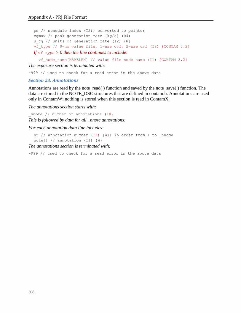
Appendix A - PRJ File Format
308
ps // schedule index (I2); converted to pointer
cgmax // peak generation rate [kg/s] (R4)
u_cg // units of generation rate (I2) {W}
vf_type // 0=no value file, 1=use cvf, 2=use dvf (I2) {CONTAM 3.2}
If vf_type > 0 then the line continues to include:
vf_node_name[NAMELEN] // value file node name (I1) {CONTAM 3.2}
The exposure section is terminated with:
-999 // used to check for a read error in the above data
Section 23: Annotations
Annotations are read by the note_read( ) function and saved by the note_save( ) function. The
data are stored in the NOTE_DSC structures that are defined in contam.h. Annotations are used
only in ContamW; nothing is stored when this section is read in ContamX.
The annotations section starts with:
_nnote // number of annotations (IX)
This is followed by data for all _nnote annotations:
For each annotation data line includes:
nr // annotation number (IX) {W}; in order from 1 to _nnode
note[] // annotation (I1) {W}
The annotations section is terminated with:
-999 // used to check for a read error in the above data
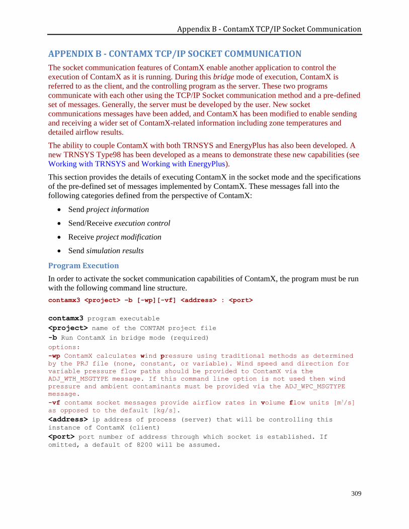
Appendix B - ContamX TCP/IP Socket Communication
309
APPENDIX B - CONTAMX TCP/IP SOCKET COMMUNICATION
The socket communication features of ContamX enable another application to control the
execution of ContamX as it is running. During this bridge mode of execution, ContamX is
referred to as the client, and the controlling program as the server. These two programs
communicate with each other using the TCP/IP Socket communication method and a pre-defined
set of messages. Generally, the server must be developed by the user. New socket
communications messages have been added, and ContamX has been modified to enable sending
and receiving a wider set of ContamX-related information including zone temperatures and
detailed airflow results.
The ability to couple ContamX with both TRNSYS and EnergyPlus has also been developed. A
new TRNSYS Type98 has been developed as a means to demonstrate these new capabilities (see
Working with TRNSYS and Working with EnergyPlus).
This section provides the details of executing ContamX in the socket mode and the specifications
of the pre-defined set of messages implemented by ContamX. These messages fall into the
following categories defined from the perspective of ContamX:
Send project information
Send/Receive execution control
Receive project modification
Send simulation results
Program Execution
In order to activate the socket communication capabilities of ContamX, the program must be run
with the following command line structure.
contamx3 <project> –b [-wp][-vf] <address> : <port>
contamx3 program executable
<project> name of the CONTAM project file
-b Run ContamX in bridge mode (required)
options:
-wp ContamX calculates wind pressure using traditional methods as determined
by the PRJ file (none, constant, or variable). Wind speed and direction for
variable pressure flow paths should be provided to ContamX via the
ADJ_WTH_MSGTYPE message. If this command line option is not used then wind
pressure and ambient contaminants must be provided via the ADJ_WPC_MSGTYPE
message.
-vf contamx socket messages provide airflow rates in volume flow units [m3/s]
as opposed to the default [kg/s].
<address> ip address of process (server) that will be controlling this
instance of ContamX (client)
<port> port number of address through which socket is established. If
omitted, a default of 8200 will be assumed.
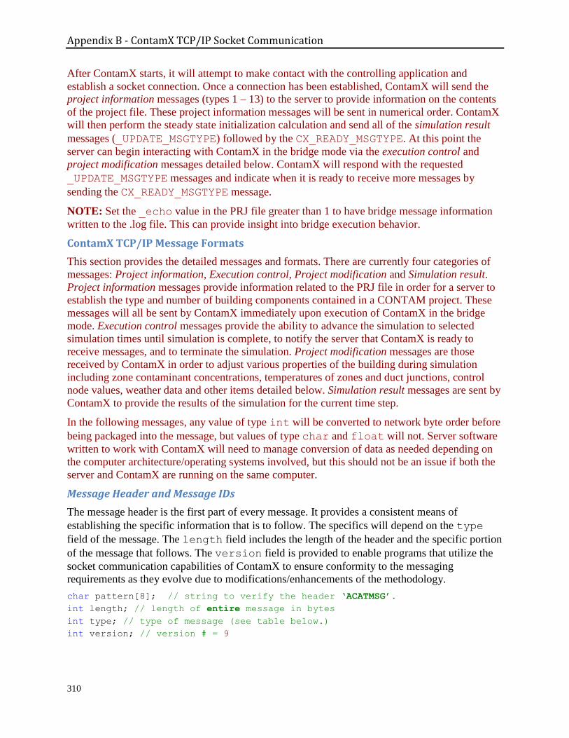
Appendix B - ContamX TCP/IP Socket Communication
310
After ContamX starts, it will attempt to make contact with the controlling application and
establish a socket connection. Once a connection has been established, ContamX will send the
project information messages (types 1 – 13) to the server to provide information on the contents
of the project file. These project information messages will be sent in numerical order. ContamX
will then perform the steady state initialization calculation and send all of the simulation result
messages (_UPDATE_MSGTYPE) followed by the CX_READY_MSGTYPE. At this point the
server can begin interacting with ContamX in the bridge mode via the execution control and
project modification messages detailed below. ContamX will respond with the requested
_UPDATE_MSGTYPE messages and indicate when it is ready to receive more messages by
sending the CX_READY_MSGTYPE message.
NOTE: Set the _echo value in the PRJ file greater than 1 to have bridge message information
written to the .log file. This can provide insight into bridge execution behavior.
ContamX TCP/IP Message Formats
This section provides the detailed messages and formats. There are currently four categories of
messages: Project information, Execution control, Project modification and Simulation result.
Project information messages provide information related to the PRJ file in order for a server to
establish the type and number of building components contained in a CONTAM project. These
messages will all be sent by ContamX immediately upon execution of ContamX in the bridge
mode. Execution control messages provide the ability to advance the simulation to selected
simulation times until simulation is complete, to notify the server that ContamX is ready to
receive messages, and to terminate the simulation. Project modification messages are those
received by ContamX in order to adjust various properties of the building during simulation
including zone contaminant concentrations, temperatures of zones and duct junctions, control
node values, weather data and other items detailed below. Simulation result messages are sent by
ContamX to provide the results of the simulation for the current time step.
In the following messages, any value of type int will be converted to network byte order before
being packaged into the message, but values of type char and float will not. Server software
written to work with ContamX will need to manage conversion of data as needed depending on
the computer architecture/operating systems involved, but this should not be an issue if both the
server and ContamX are running on the same computer.
Message Header and Message IDs
The message header is the first part of every message. It provides a consistent means of
establishing the specific information that is to follow. The specifics will depend on the type
field of the message. The length field includes the length of the header and the specific portion
of the message that follows. The version field is provided to enable programs that utilize the
socket communication capabilities of ContamX to ensure conformity to the messaging
requirements as they evolve due to modifications/enhancements of the methodology.
char pattern[8]; // string to verify the header ‘ACATMSG’.
int length; // length of entire message in bytes
int type; // type of message (see table below.)
int version; // version # = 9
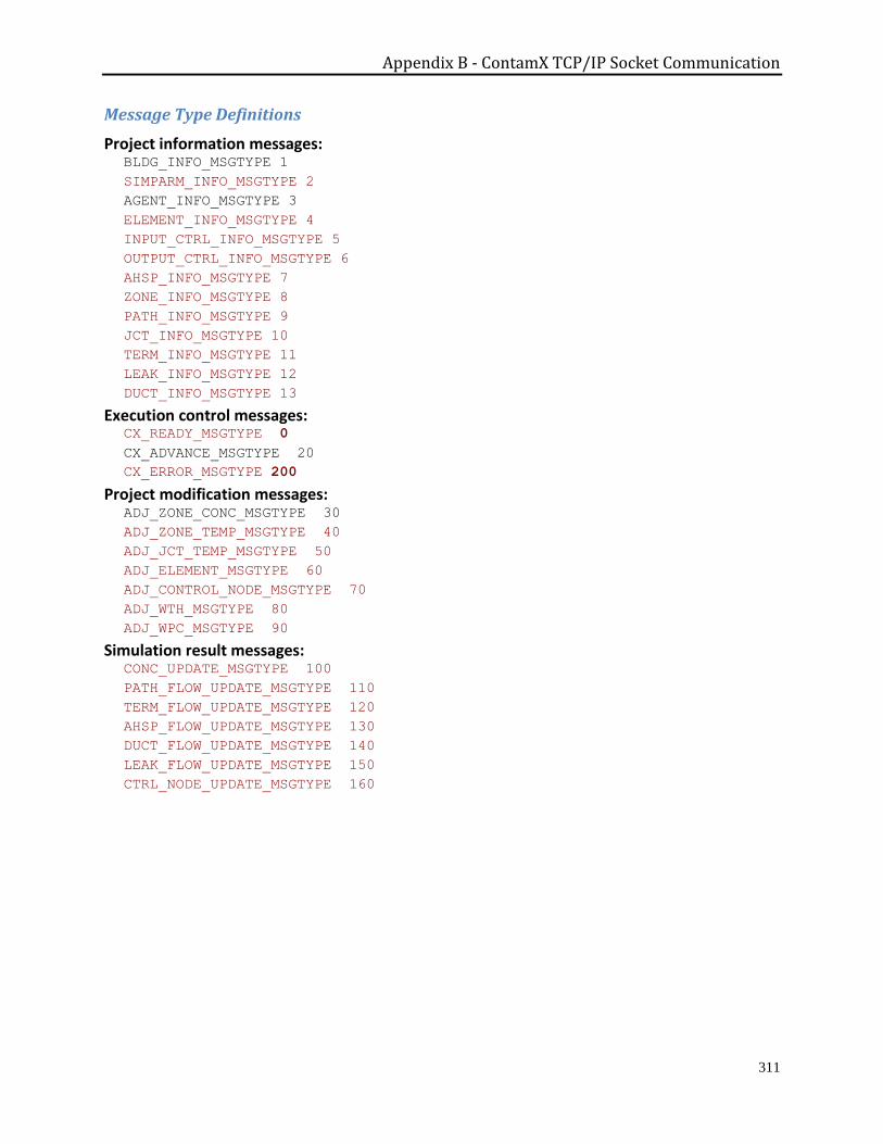
Appendix B - ContamX TCP/IP Socket Communication
311
Message Type Definitions
Project information messages: BLDG_INFO_MSGTYPE 1
SIMPARM_INFO_MSGTYPE 2
AGENT_INFO_MSGTYPE 3
ELEMENT_INFO_MSGTYPE 4
INPUT_CTRL_INFO_MSGTYPE 5
OUTPUT_CTRL_INFO_MSGTYPE 6
AHSP_INFO_MSGTYPE 7
ZONE_INFO_MSGTYPE 8
PATH_INFO_MSGTYPE 9
JCT_INFO_MSGTYPE 10
TERM_INFO_MSGTYPE 11
LEAK_INFO_MSGTYPE 12
DUCT_INFO_MSGTYPE 13
Execution control messages: CX_READY_MSGTYPE 0
CX_ADVANCE_MSGTYPE 20
CX_ERROR_MSGTYPE 200
Project modification messages: ADJ_ZONE_CONC_MSGTYPE 30
ADJ_ZONE_TEMP_MSGTYPE 40
ADJ_JCT_TEMP_MSGTYPE 50
ADJ_ELEMENT_MSGTYPE 60
ADJ_CONTROL_NODE_MSGTYPE 70
ADJ_WTH_MSGTYPE 80
ADJ_WPC_MSGTYPE 90
Simulation result messages: CONC_UPDATE_MSGTYPE 100
PATH_FLOW_UPDATE_MSGTYPE 110
TERM_FLOW_UPDATE_MSGTYPE 120
AHSP_FLOW_UPDATE_MSGTYPE 130
DUCT_FLOW_UPDATE_MSGTYPE 140
LEAK_FLOW_UPDATE_MSGTYPE 150
CTRL_NODE_UPDATE_MSGTYPE 160
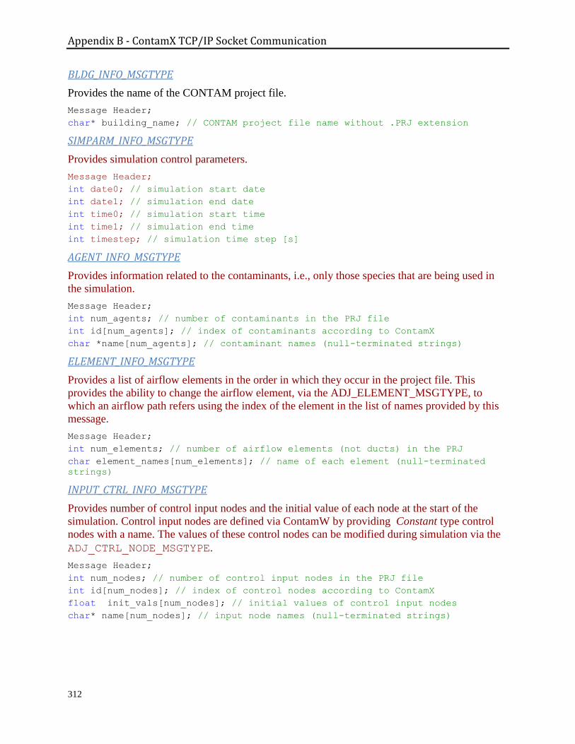
Appendix B - ContamX TCP/IP Socket Communication
312
BLDG_INFO_MSGTYPE
Provides the name of the CONTAM project file.
Message Header;
char* building_name; // CONTAM project file name without .PRJ extension
SIMPARM_INFO_MSGTYPE
Provides simulation control parameters.
Message Header;
int date0; // simulation start date
int date1; // simulation end date
int time0; // simulation start time
int time1; // simulation end time
int timestep; // simulation time step [s]
AGENT_INFO_MSGTYPE
Provides information related to the contaminants, i.e., only those species that are being used in
the simulation.
Message Header;
int num_agents; // number of contaminants in the PRJ file
int id[num_agents]; // index of contaminants according to ContamX
char *name[num_agents]; // contaminant names (null-terminated strings)
ELEMENT_INFO_MSGTYPE
Provides a list of airflow elements in the order in which they occur in the project file. This
provides the ability to change the airflow element, via the ADJ_ELEMENT_MSGTYPE, to
which an airflow path refers using the index of the element in the list of names provided by this
message.
Message Header;
int num_elements; // number of airflow elements (not ducts) in the PRJ
char element_names[num_elements]; // name of each element (null-terminated
strings)
INPUT_CTRL_INFO_MSGTYPE
Provides number of control input nodes and the initial value of each node at the start of the
simulation. Control input nodes are defined via ContamW by providing Constant type control
nodes with a name. The values of these control nodes can be modified during simulation via the
ADJ_CTRL_NODE_MSGTYPE.
Message Header;
int num_nodes; // number of control input nodes in the PRJ file
int id[num_nodes]; // index of control nodes according to ContamX
float init_vals[num_nodes]; // initial values of control input nodes
char* name[num_nodes]; // input node names (null-terminated strings)
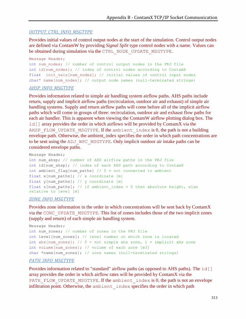
Appendix B - ContamX TCP/IP Socket Communication
313
OUTPUT_CTRL_INFO_MSGTYPE
Provides initial values of control output nodes at the start of the simulation. Control output nodes
are defined via ContamW by providing Signal Split type control nodes with a name. Values can
be obtained during simulation via the CTRL_NODE_UPDATE_MSGTYPE.
Message Header;
int num_nodes; // number of control output nodes in the PRJ file
int id[num_nodes]; // index of control nodes according to ContamX
float init_vals[num_nodes]; // initial values of control input nodes
char* name[num_nodes]; // output node names (null-terminated strings)
AHSP_INFO_MSGTYPE
Provides information related to simple air handling system airflow paths. AHS paths include
return, supply and implicit airflow paths (recirculation, outdoor air and exhaust) of simple air
handling systems. Supply and return airflow paths will come before all of the implicit airflow
paths which will come in groups of three: recirculation, outdoor air and exhaust flow paths for
each air handler. This is apparent when viewing the ContamW airflow plotting dialog box. The
id[] array provides the order in which airflows will be provided by ContamX via the
AHSP_FLOW_UPDATE_MSGTYPE. If the ambient_index is 0, the path is not a building
envelope path. Otherwise, the ambient_index specifies the order in which path concentrations are
to be sent using the ADJ_WPC_MSGTYPE. Only implicit outdoor air intake paths can be
considered envelope paths.
Message Header;
int num_ahsp; // number of AHS airflow paths in the PRJ file
int id[num_ahsp]; // index of each AHS path according to ContamX
int ambient_flag[num_paths] // 0 = not connected to ambient
float x[num_paths]; // x coordinate [m]
float y[num_paths]; // y coordinate [m]
float z[num_paths]; // if ambient_index > 0 then absolute height, else
relative to level [m]
ZONE_INFO_MSGTYPE
Provides zone information in the order in which concentrations will be sent back by ContamX
via the CONC_UPDATE_MSGTYPE. This list of zones includes those of the two implicit zones
(supply and return) of each simple air handling system.
Message Header;
int num_zones; // number of zones in the PRJ file
int level[num_zones]; // level number on which zone is located
int ahs[num_zones]; // 0 = not simple ahs zone, 1 = implicit ahs zone
int volume[num_zones]; // volume of each zone [m3]
char *name[num_zones]; // zone names (null-terminated strings)
PATH_INFO_MSGTYPE
Provides information related to "standard" airflow paths (as opposed to AHS paths). The id[]
array provides the order in which airflow rates will be provided by ContamX via the
PATH_FLOW_UPDATE_MSGTYPE. If the ambient_index is 0, the path is not an envelope
infiltration point. Otherwise, the ambient_index specifies the order in which path

Appendix B - ContamX TCP/IP Socket Communication
314
concentrations are to be sent using the ADJ_WPC_MSGTYPE. Positive flow direction is based on
airflow path data to be from zone n to zone m.
Message Header;
int num_paths; // number of airflow paths in the PRJ
int id[num_paths]; // index according to ContamX
int ambient_index[num_paths] // 0 = not connected to ambient
int element_index[num_paths]; // index of initial airflow element
int from_zone[num_paths]; // zone number of from zone (based on positive flow
direction)
int to_zone[num_paths]; // zone number of to zone
float x[num_paths]; // x coordinate [m]
float y[num_paths]; // y coordinate [m]
float z[num_paths]; // if ambient_index > 0 then absolute height, else
relative to level [m]
JCT_INFO_MSGTYPE
Provides the number of junctions and the type of each junction. The index of the type[] array
is used to set the temperature of the junctions via the ADJ_JCT_TEMP_MSGTYPE.
Message Header;
int num_jcts; // number of junctions in the PRJ file
int type[num_jcts]; // junction type: 0=junction, 1=terminal
TERM_INFO_MSGTYPE
Provides information on those junctions that are terminal types. The id[] array provides the order
in which airflow rates will be provided by ContamX via TERM_FLOW_UPDATE_MSGTYPE. If
the ambient_index is 0, this terminal is not an infiltration point. Otherwise, ambient_index
specifies the order in which terminal concentrations are to be sent to ContamX using
ADJ_WPC_MSGTYPE.
Message Header;
int num_terms; // number of duct terminals in the PRJ
int id[num_terms]; // for each terminal: index according to ContamX
int ambient_index[num_terms] // for each terminal: 0/1 = not connected /
connected to ambient
float x[num_terms]; // for each terminal: absolute coordinates [m]
float y[num_terms];
float z[num_terms];
LEAK_INFO_MSGTYPE
Provides a list of only those duct junctions which have been defined via ContamW to have
leakage. The id[] array provides the order in which airflow rates will be provided by ContamX
via LEAK_FLOW_UPDATE_MSGTYPE. Currently leaks are not included when using
ADJ_WPC_MSGTYPE., so ambient_index will be zero for all leaks.
Message Header;
int num_leaks; // number of junctions with leaks in the PRJ
int id[num_leaks]; // index according to ContamX
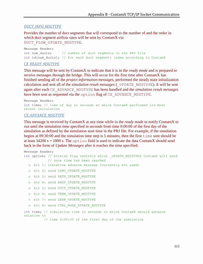
Appendix B - ContamX TCP/IP Socket Communication
315
DUCT_INFO_MSGTYPE
Provides the number of duct segments that will correspond to the number of and the order in
which duct segment airflow rates will be sent by ContamX via
DUCT_FLOW_UPDATE_MSGTYPE.
Message Header;
int num_ducts; // number of duct segments in the PRJ file
int id[num_ducts]; // for each duct segment: index according to ContamX
CX_READY_MSGTYPE
This message will be sent by ContamX to indicate that it is in the ready mode and is prepared to
receive messages through the bridge. This will occur for the first time after ContamX has
finished sending all of the project information messages, performed the steady state initialization
calculation and sent all of the simulation result messages (_UPDATE_MSGTYPE). It will be sent
again after each CX_ADVANCE_MSGTYPE has been handled and the simulation result messages
have been sent as requested via the option flag of CX_ADVANCE_MSGTYPE.
Message Header;
int time; // time of day in seconds at which ContamX performed its most
recent calculation
CX_ADVANCE_MSGTYPE
This message is received by ContamX at any time while in the ready mode to notify ContamX to
run until the simulation time specified in seconds from time 0:00:00 of the first day of the
simulation as defined by the simulation start time in the PRJ file. For example, if the simulation
begins at 09:30:00 and the simulation time step is 5 minutes, then the first time sent should be
at least 34200 s + 1800 s. The option field is used to indicate the data ContamX should send
back in the form of Update Messages after it reaches the time specified.
Message Header;
int option; // bitwise flag controls which _UPDATE_MSGTYPES ContamX will send
// once time has been reached
o bit 1: iterative advance message (currently not used)
o bit 2: send CONC_UPDATE_MSGTYPE
o bit 3: send PATH_UPDATE_MSGTYPE
o bit 4: send AHSP_UPDATE_MSGTYPE
o bit 5: send DUCT_UPDATE_MSGTYPE
o bit 6: send TERM_UPDATE_MSGTYPE
o bit 7: send LEAK_UPDATE_MSGTYPE
o bit 8: send CTRL_NODE_UPDATE_MSGTYPE
int time; // simulation time in seconds to which ContamX should advance
relative to
// time 0:00:00 of the first day of the simulation
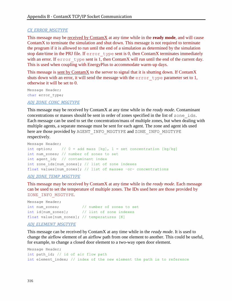
Appendix B - ContamX TCP/IP Socket Communication
316
CX_ERROR_MSGTYPE
This message may be received by ContamX at any time while in the ready mode, and will cause
ContamX to terminate the simulation and shut down. This message is not required to terminate
the program if it is allowed to run until the end of a simulation as determined by the simulation
stop date/time in the PRJ file. If error_type sent is 0, then ContamX terminates immediately
with an error. If error_type sent is 1, then ContamX will run until the end of the current day.
This is used when coupling with EnergyPlus to accommodate warm-up days.
This message is sent by ContamX to the server to signal that it is shutting down. If ContamX
shuts down with an error, it will send the message with the error_type parameter set to 1,
otherwise it will be set to 0.
Message Header;
char error_type;
ADJ_ZONE_CONC_MSGTYPE
This message may be received by ContamX at any time while in the ready mode. Contaminant
concentrations or masses should be sent in order of zones specified in the list of zone_ids.
Each message can be used to set the concentration/mass of multiple zones, but when dealing with
multiple agents, a separate message must be sent for each agent. The zone and agent ids used
here are those provided by AGENT_INFO_MSGTYPE and ZONE_INFO_MSGTYPE
respectively.
Message Header;
int option; // 0 = add mass [kg], 1 = set concentration [kg/kg]
int num_zones; // number of zones to set
int agent_id; // contaminant index
int zone_ids[num_zones]; // list of zone indexes
float values[num_zones]; // list of masses –or- concentrations
ADJ_ZONE_TEMP_MSGTYPE
This message may be received by ContamX at any time while in the ready mode. Each message
can be used to set the temperature of multiple zones. The IDs used here are those provided by
ZONE_INFO_MSGTYPE.
Message Header;
int num_zones; // number of zones to set
int id[num_zones]; // list of zone indexes
float value[num_zones]; // temperatures [K]
ADJ_ELEMENT_MSGTYPE
This message can be received by ContamX at any time while in the ready mode. It is used to
change the airflow element of an airflow path from one element to another. This could be useful,
for example, to change a closed door element to a two-way open door element.
Message Header;
int path_id; // id of air flow path
int element_index; // index of the new element the path is to reference
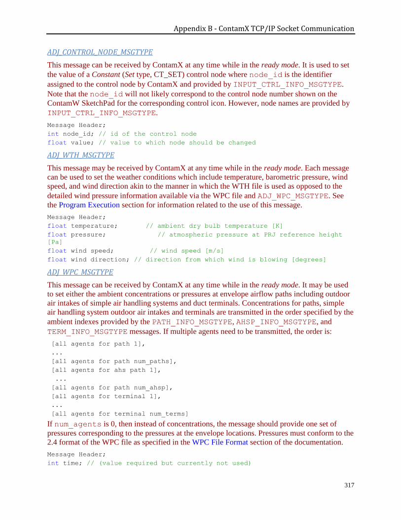
Appendix B - ContamX TCP/IP Socket Communication
317
ADJ_CONTROL_NODE_MSGTYPE
This message can be received by ContamX at any time while in the ready mode. It is used to set
the value of a Constant (Set type, CT_SET) control node where node_id is the identifier
assigned to the control node by ContamX and provided by INPUT_CTRL_INFO_MSGTYPE.
Note that the node_id will not likely correspond to the control node number shown on the
ContamW SketchPad for the corresponding control icon. However, node names are provided by
INPUT_CTRL_INFO_MSGTYPE.
Message Header;
int node_id; // id of the control node
float value; // value to which node should be changed
ADJ_WTH_MSGTYPE
This message may be received by ContamX at any time while in the ready mode. Each message
can be used to set the weather conditions which include temperature, barometric pressure, wind
speed, and wind direction akin to the manner in which the WTH file is used as opposed to the
detailed wind pressure information available via the WPC file and ADJ_WPC_MSGTYPE. See
the Program Execution section for information related to the use of this message.
Message Header;
float temperature; // ambient dry bulb temperature [K]
float pressure; // atmospheric pressure at PRJ reference height
[Pa]
float wind speed; // wind speed [m/s]
float wind direction; // direction from which wind is blowing [degrees]
ADJ_WPC_MSGTYPE
This message can be received by ContamX at any time while in the ready mode. It may be used
to set either the ambient concentrations or pressures at envelope airflow paths including outdoor
air intakes of simple air handling systems and duct terminals. Concentrations for paths, simple
air handling system outdoor air intakes and terminals are transmitted in the order specified by the
ambient indexes provided by the PATH_INFO_MSGTYPE, AHSP_INFO_MSGTYPE, and
TERM_INFO_MSGTYPE messages. If multiple agents need to be transmitted, the order is:
[all agents for path 1],
...
[all agents for path num_paths],
[all agents for ahs path 1],
...
[all agents for path num_ahsp],
[all agents for terminal 1],
...
[all agents for terminal num_terms]
If num_agents is 0, then instead of concentrations, the message should provide one set of
pressures corresponding to the pressures at the envelope locations. Pressures must conform to the
2.4 format of the WPC file as specified in the WPC File Format section of the documentation.
Message Header;
int time; // (value required but currently not used)
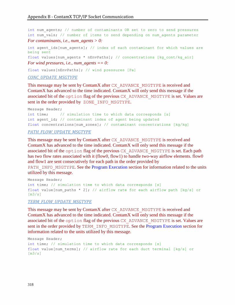
Appendix B - ContamX TCP/IP Socket Communication
318
int num_agents; // number of contaminants OR set to zero to send pressures
int num_vals; // number of items to send depending on num_agents parameter
For contaminants, i.e., num_agents > 0:
int agent_ids[num_agents]; // index of each contaminant for which values are
being sent
float values[num_agents * nEnvPaths]; // concentrations [kg_cont/kg_air]
For wind pressures, i.e., num_agents == 0:
float values[nEnvPaths]; // wind pressures [Pa]
CONC_UPDATE_MSGTYPE
This message may be sent by ContamX after CX_ADVANCE_MSGTYPE is received and
ContamX has advanced to the time indicated. ContamX will only send this message if the
associated bit of the option flag of the previous CX_ADVANCE_MSGTYPE is set. Values are
sent in the order provided by ZONE_INFO_MSGTYPE.
Message Header;
int time; // simulation time to which data corresponds [s]
int agent_id; // contaminant index of agent being updated
float concentrations[num_zones]; // contaminant concentrations [kg/kg]
PATH_FLOW_UPDATE_MSGTYPE
This message may be sent by ContamX after CX_ADVANCE_MSGTYPE is received and
ContamX has advanced to the time indicated. ContamX will only send this message if the
associated bit of the option flag of the previous CX_ADVANCE_MSGTYPE is set. Each path
has two flow rates associated with it (flow0, flow1) to handle two-way airflow elements. flow0
and flow1 are sent consecutively for each path in the order provided by
PATH_INFO_MSGTYPE. See the Program Execution section for information related to the units
utilized by this message.
Message Header;
int time; // simulation time to which data corresponds [s]
float value[num_paths * 2]; // airflow rate for each airflow path [kg/s] or
[m3/s]
TERM_FLOW_UPDATE_MSGTYPE
This message may be sent by ContamX after CX_ADVANCE_MSGTYPE is received and
ContamX has advanced to the time indicated. ContamX will only send this message if the
associated bit of the option flag of the previous CX_ADVANCE_MSGTYPE is set. Values are
sent in the order provided by TERM_INFO_MSGTYPE. See the Program Execution section for
information related to the units utilized by this message.
Message Header;
int time; // simulation time to which data corresponds [s]
float value[num_terms]; // airflow rate for each duct terminal [kg/s] or
[m3/s]
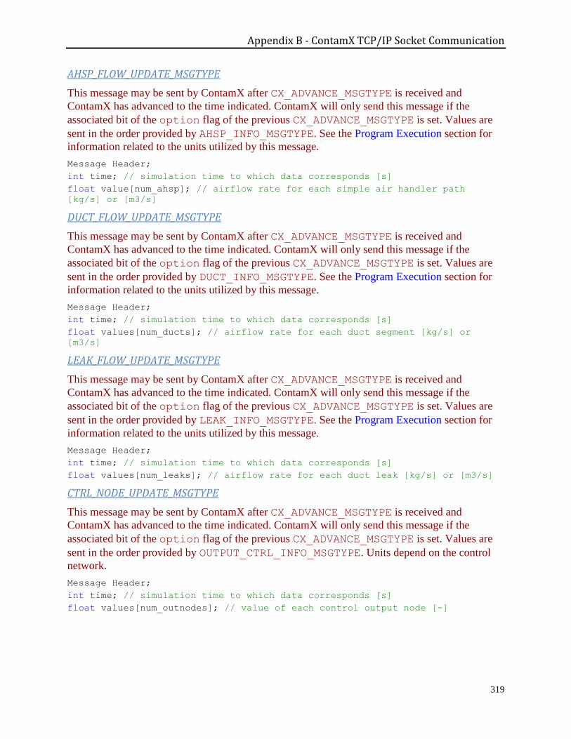
Appendix B - ContamX TCP/IP Socket Communication
319
AHSP_FLOW_UPDATE_MSGTYPE
This message may be sent by ContamX after CX_ADVANCE_MSGTYPE is received and
ContamX has advanced to the time indicated. ContamX will only send this message if the
associated bit of the option flag of the previous CX_ADVANCE_MSGTYPE is set. Values are
sent in the order provided by AHSP_INFO_MSGTYPE. See the Program Execution section for
information related to the units utilized by this message.
Message Header;
int time; // simulation time to which data corresponds [s]
float value[num_ahsp]; // airflow rate for each simple air handler path
[kg/s] or [m3/s]
DUCT_FLOW_UPDATE_MSGTYPE
This message may be sent by ContamX after CX_ADVANCE_MSGTYPE is received and
ContamX has advanced to the time indicated. ContamX will only send this message if the
associated bit of the option flag of the previous CX_ADVANCE_MSGTYPE is set. Values are
sent in the order provided by DUCT_INFO_MSGTYPE. See the Program Execution section for
information related to the units utilized by this message.
Message Header;
int time; // simulation time to which data corresponds [s]
float values[num_ducts]; // airflow rate for each duct segment [kg/s] or
[m3/s]
LEAK_FLOW_UPDATE_MSGTYPE
This message may be sent by ContamX after CX_ADVANCE_MSGTYPE is received and
ContamX has advanced to the time indicated. ContamX will only send this message if the
associated bit of the option flag of the previous CX_ADVANCE_MSGTYPE is set. Values are
sent in the order provided by LEAK_INFO_MSGTYPE. See the Program Execution section for
information related to the units utilized by this message.
Message Header;
int time; // simulation time to which data corresponds [s]
float values[num_leaks]; // airflow rate for each duct leak [kg/s] or [m3/s]
CTRL_NODE_UPDATE_MSGTYPE
This message may be sent by ContamX after CX_ADVANCE_MSGTYPE is received and
ContamX has advanced to the time indicated. ContamX will only send this message if the
associated bit of the option flag of the previous CX_ADVANCE_MSGTYPE is set. Values are
sent in the order provided by OUTPUT_CTRL_INFO_MSGTYPE. Units depend on the control
network.
Message Header;
int time; // simulation time to which data corresponds [s]
float values[num_outnodes]; // value of each control output node [-]