Contagion in Financial Systems: A Bayesian Network Approach fileSIAM J. FINANCIAL MATH. c 2018 Society for Industrial and Applied Mathematics Vol. 9, No. 1, pp. 28{53 Contagion in

SIAM J. FINANCIAL MATH. c© 2018 Society for Industrial and Applied MathematicsVol. 9, No. 1, pp. 28–53

Contagion in Financial Systems: A Bayesian Network Approach∗

Carsten Chong† and Claudia Kluppelberg†

Abstract. We develop a structural default model for interconnected financial institutions in a probabilisticframework. For all possible network structures we characterize the joint default distribution of thesystem using Bayesian network methodologies. Particular emphasis is given to the treatment andconsequences of cyclic financial linkages. We further demonstrate how Bayesian network theorycan be applied to detect contagion channels within the financial network, to measure the systemicimportance of selected entities on others, and to compute conditional or unconditional probabilitiesof default for single or multiple institutions.

Key words. Bayesian network, financial contagion, measure of systemic risk, multivariate default risk, proba-bility of default, structural default risk model, systemic risk

AMS subject classifications. 91B30, 62-09, 91G80

DOI. 10.1137/17M1116659

1. Introduction. The 2007–2008 financial crisis has unmistakably revealed on which frag-ile grounds the global financial system was built at that time. Contrary to the usual perceptionthat diversification reduces risk, it was precisely the interconnectedness of the system thatmade the spread of shocks across large scales possible. Henceforth, a lot of effort has been putinto understanding the origin, the mechanisms, and the consequences of financial contagion. Itis still a matter of current research to analyze the complex effects of financial interconnectionand whether it is a blessing or a curse for the stability of the overall financial system. Forexample, while the classical papers by Allen and Gale (2000) and Freixas, Parigi, and Rochet(2000) argue that interconnection strengthens the resilience of financial systems, recent workby Acemoglu, Ozdaglar, and Tahbaz-Salehi (2015) and Elliott, Golub, and Jackson (2014)demonstrate the robust yet fragile nature of financial systems: Densely connected systemscan prove to be more robust but also to be more vulnerable to shocks depending on the actualnetwork structure. Therefore, a profound understanding of interconnectedness and the risk offinancial contagion is inevitable for bankers, regulators, and other decision makers in order toset up effective detection and prevention mechanisms for possible future crises.

In the literature on balance sheet contagion, one of the most prominent default cascademodels is that of Eisenberg and Noe (2001). Under mild assumptions on the operative cashflows the financial institutions generate, the authors use a fixed-point argument to estab-lish the existence of a unique clearing payment vector, which can be explicitly computedvia a fictitious default algorithm. Extending the model by introducing bankruptcy costs,

∗Received by the editors February 15, 2017; accepted for publication (in revised form) July 14, 2017; publishedelectronically January 11, 2018.

http://www.siam.org/journals/sifin/9-1/M111665.html†Center for Mathematical Sciences, Technical University of Munich, 85748 Garching, Germany (carsten.chong@

tum.de, [email protected], www.statistics.ma.tum.de).

28

http://www.siam.org/journals/sifin/9-1/M111665.html

mailto:[email protected]



www.statistics.ma.tum.de

CONTAGION: A BAYESIAN NETWORK APPROACH 29

Rogers and Veraart (2013) show that the clearing vector is no longer uniquely determinedin general. Instead, the fictitious default algorithm can be modified to produce the greatestand the least clearing vector. Although Eisenberg and Noe (2001) also discuss qualitativeimplications of stochastic operative cash flows, the core analysis of these two papers remainsdeterministic.

Imposing maximal bankruptcy costs (i.e., creditors lose the total value of a claim upondefault of the counterparty), Gai and Kapadia (2010) show that the relationship betweenconnectedness and stability in financial systems exhibits a phase transition: Interconnectioncan both absorb and amplify shocks. Analytical results, however, are only obtained on ho-mogeneous random graphs where exposures are evenly distributed among all counterparties.We refer to Hurd (2016) for extensions and comparisons between the Eisenberg–Noe and theGai–Kapadia model.

A nonmonotonic effect of interconnection on stability is also confirmed by Acemoglu,Ozdaglar, and Tahbaz-Salehi (2015). Drawing on a variant of Eisenberg and Noe’s model, theyshow that for small shocks, highly diversified systems are less susceptible to contagion thansparsely connected networks but that the opposite is true for big shocks. Methodologically,the authors impose a two-state evolution for the firms and identify the optimal network forthe small as well as the big shock regime. Assuming that interconnection arises through assetcross-holdings rather than mutual liabilities, Elliott, Golub, and Jackson (2014) derive thesame qualitative result on various random graph models.

Another interesting development of the Eisenberg–Noe model is carried out by Gourieroux,Heam, and Monfort (2012). The authors first extend the existence and uniqueness of a clearingvector to the situation where interfirm share holdings are included in the model. Additional tothese (again purely deterministic) considerations, they further discuss the consequences for thefinancial system when random shocks occur, giving two quantitative results. First, they com-pute the conditional distribution of the firm values when it is known which firms default andwhich not. Second, they provide an enumeration-type formula for the probability of defaultfor a given firm in the network. However, they do not reveal how the terms in their expansion(which are the probabilities of joint default configurations) can be computed. Furthermore,it is unclear how to determine which institutions default or not at first place because this inturn depends on the firm values. Finally, let us also mention Glasserman and Young (2015),who give quantitative estimates on the probability of default in various contagion models.

In addition to the mainly theoretical contributions mentioned above, a lot of empiricalwork has been carried out; see, e.g., Elsinger, Lehar, and Summer (2006), Cont, Moussa, andSantos (2013), Craig and von Peter (2014), and Langfield, Liu, and Ota (2014) for applica-tions to central bank data from the Austrian, Brazilian, German, and UK banking system,respectively. Furthermore, apart from work based on variations of the Eisenberg and Noe(2001) model, there are also other network-based approaches to systemic risk. We refer toCastiglionesi and Eboli (2015) for the usage of flow network techniques, to Fouque and Sun(2013), Kley, Kluppelberg, and Reichel (2015), and Chong and Kluppelberg (2017) for mod-els relying on stochastic differential equations, and to Amini, Cont, and Minca (2016) andDetering et al. (2017) for contagion analyses on large random graphs. While the analysis inCastiglionesi and Eboli (2015) is again deterministic, the other papers rely on probabilisticapproaches that only apply to stylized or limiting networks.

30 CARSTEN CHONG AND CLAUDIA KLUPPELBERG

Even though some of the aforementioned works discuss stochastic effects in the contextof financial contagion, the full structure of the default probabilities within a given (not nec-essarily stylized) financial system remains unknown when future returns are random. Andthis is exactly the problem we want to address in the present paper. For all possible networkstructures of a financial system subjected to stochastic shocks, we give a complete characteri-zation of the joint default probability distribution of the system in a way that the probabilityof default for a single institution or a group of institutions can be computed efficiently. More-over, our analysis will also allow for identifying possible channels of financial contagion andmeasuring the systemic importance of institutions.

Our approach will draw upon methods from the theory of Bayesian networks, also knownas directed graphical models; see, e.g., Lauritzen (1996) and Koller and Friedman (2009). Thesemodels are a priori defined on directed acyclic graphs (DAGs), but it is widely aknowledgedthat mutual dependencies and directed cycles are omnipresent in financial systems. Therefore,for the purposes of this paper, we have to extend the theory of Bayesian networks to graphswith directed cycles, and we will do so by interpreting a cyclic model as the margin of anacyclic model on a suitably enlarged graph. This methodology for treating cyclic graphicalmodels or, more generally, systems with feedback cycles is of independent interest and maybe useful for other applications as well.

The remaining article is organized as follows. In section 2, we introduce a probabilisticstructural default model for interconnected financial institutions. As in Gai and Kapadia(2010), Rogers and Veraart (2013), and Elliott, Golub, and Jackson (2014), our model takesbankruptcy costs into account so that the standard balance sheet equations may no longerhave a unique solution. Apart from specific examples, a general characterization of uniquenessof solutions seems to be absent in the literature. So this leads to our first main result,Theorem 2.4, which states that uniqueness holds if and only if the underlying liability networkcorresponds to a DAG.

If the interfirm liabilities exhibit a DAG structure, we further prove in section 3, Theo-rem 3.2, that the default variables of the institutions form a Bayesian network on this DAG. Inother words, if we fix an institution i and assume knowledge about the state of all its debtors(its parents in the language of graph theory), its default probability is independent of all otherfirms that have not lent (directly or indirectly via other firms) to i (the nondescendants of i).

If there are directed lending cycles, which is most likely the case in practice, the previouslyidentified nonuniqueness problem requires further specification of the sets of defaulting andsurviving firms. For the two extremal cases, the mild and the strict default rule, we recover inTheorems 3.10 and 3.12 the Bayesian network structure of the default variables on a suitablyenlarged liability graph. So for all financial networks—no matter with or without directedcycles—the joint default distribution of the system can be efficiently structured in terms of aBayesian network.

In section 4, we discuss the practical consequences and advantages of having a Bayesiannetwork structure. We first reveal how to decide on a graphical basis whether the default of two(or two groups of) firms is stochastically dependent or not. Second, we highlight in a numericalstudy how established algorithms can be used to compute conditional or unconditional defaultprobabilities, either exactly or approximatively. Finally, we define and analyze two measuresof systemic risk that follow from our Bayesian network analysis. In contrast to many already


existing measures, ours are probabilistic in nature and follow from a structural default cascademodel. Section 5 concludes and points at further research directions.

2. Default risk model for interconnected firms. We considerN firms labeled i = 1, . . . , Nwithin an economy for a single period. At time t = 0, each firm i has some operating assets Xi

and some cash Ki that yields a riskless continuous interest at a rate of r0. The same firm alsohas some external liabilities Fi that are to be redeemed at time t = T , the end of the period,with a continuous interest rate of r′0. In addition to that, at t = 0, each firm i has lent firmj an amount of Lij (possibly 0) which is to be repaid by j at time t = T with a continuousinterest rate of rij . In other words, firm i holds a bond of firm j with face value Lij and asingle coupon payment at maturity T . Apart from that, no other financial involvement existsbetween the N firms.

During the period from t = 0 to t = T every company i uses its operating assets Xi torun a firm-specific business. Following the classical work of Merton (1974), this is assumedto evolve according to a geometric Brownian motion with drift µi and volatility σ2

i . Thedriving Brownian motions B1, . . . , BN are considered to be independent. We shall commenton possible relaxations of this assumption in section 5.

In order to simplify the subsequent exposition, the values Ki, Fi, and Lij are assumed tobe nonnegative; the asset drifts µi as well as the interest rates rij , r0, and r′0 may take positiveor negative values; and Xi, σi, and T are strictly positive. Moreover, for each i ∈ {1, . . . , N}we suppose that

(2.1) Ki < e(r′0−r0)TFi +N∑j=1

e(rji−r0)TLji.

Firms that have more cash reserves than the bound on the right-hand side of (2.1) will neverexperience default at time t = T . Even if they do not receive payments from the otherinstitutions and lose all their operating assets, they still have enough money to meet all theirobligations. Since we are interested in the default probabilities within the financial network,there is no loss of generality if we exclude such institutions from our analysis.

Let us also point out that we take a “central bank” perspective in this paper. All pa-rameters and quantities introduced above are assumed to be known or have been estimatedbefore. We refer to Anand, Craig, and von Peter (2015), Gandy and Veraart (2016), andUpper (2011) for various methods to estimate interfirm exposures.

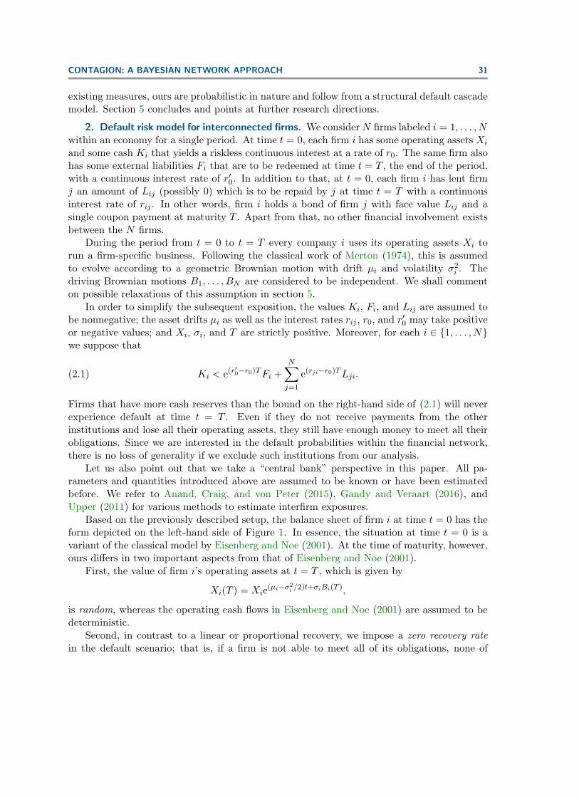
Based on the previously described setup, the balance sheet of firm i at time t = 0 has theform depicted on the left-hand side of Figure 1. In essence, the situation at time t = 0 is avariant of the classical model by Eisenberg and Noe (2001). At the time of maturity, however,ours differs in two important aspects from that of Eisenberg and Noe (2001).

First, the value of firm i’s operating assets at t = T , which is given by

Xi(T ) = Xie(µi−σ2i /2)t+σiBi(T ),

is random, whereas the operating cash flows in Eisenberg and Noe (2001) are assumed to bedeterministic.

Second, in contrast to a linear or proportional recovery, we impose a zero recovery ratein the default scenario; that is, if a firm is not able to meet all of its obligations, none of


Operating assets Liabilities- external

Xi Fi

Loans - to other firmsN∑j=1

Lij

N∑j=1

Lji

Cash EquityKi Ei(0)

Assets at t = 0 Liabilities and eq-uity at t = 0

Operating assets Liabilities- external

Xi(T ) er′0TFi

Loans - to other firmsN∑j=1

erijTLij1S(j)N∑j=1

erjiTLji

Cash Equityer0TKi Ei(T )

Assets at t = T Liabilities and eq-uity at t = T

Figure 1. Idealized balance sheet of firm i at t = 0 and t = T .

its creditors receives any payment. As Gai and Kapadia (2010) argue, “This assumption islikely to be realisitic in the midst of a crisis: In the immediate aftermath of a default, therecovery rate and the timing of recovery will be highly uncertain and banks’ funders are likelyto assume the worst-case scenario” (p. 2407). We also refer to Battiston et al. (2012) andCont, Moussa, and Santos (2013) for a similar reasoning and Memmel, Sachs, and Stein (2012)for empirical evidence for the frequent occurrence of a recovery rate close to zero.

Standard balance sheet considerations lead us to the following definition (we do not dis-tinguish between the terms bankruptcy, default, and insolvency in this paper).

Definition 2.1. A company defaults ( survives) at time t = T if it belongs to the set

(2.2) D := {i ∈ {1, . . . , N} : Ei(T ) < 0}(S := {i ∈ {1, . . . , N} : Ei(T ) ≥ 0}

),

where Ei(T ) is the equity of firm i at time T given by

(2.3) Ei(T ) := Xi(T ) +N∑j=1

erijTLij1S(j) + er0TKi − er′0TFi −

N∑j=1

erjiTLji.

Moreover, we define

Di := 1D(i), Si := 1−Di = 1S(i), i = 1, . . . , N.

The resulting balance sheets at time t = T are depicted on the right-hand side of Figure 1.As a consequence of the stochasticity of the asset values Xi(T ), the equity values Ei(T ), the


sets D and S and the variables Di and Si are random. The natural question arises whetherthe knowledge of X1(T ), . . . , XN (T ) at time T fully determines D, S and Ei(T ) throughequations (2.2) and (2.3). In the model of Eisenberg and Noe (2001) the existence anduniqueness of solutions to (2.2) and (2.3) would immediately follow from the strict positivityof all Xi(T ). This condition, however, is no longer sufficient for uniqueness under the zerorecovery assumption as the following simple counterexample demonstrates.

Example 2.2. Suppose there are two firms in the system owing each other $10 at maturitywith neither cash deposits nor external liabilities. If both firms have realized operating assetsamounting to X1(T ) = X2(T ) = $5 at t = T , there are two different solutions to equations(2.2) and (2.3):

(1) D = {1, 2}, S = ∅, and E1(T ) = E2(T ) = −$5 and(2) D = ∅, S = {1, 2}, and E1(T ) = E2(T ) = $5.

The emergence of multiple solutions in the previous example highlights the remainingpoint of indeterminancy in our model: To what extent is clearing between distressed firms or,more precisely, the netting of mutual claims allowed? In the first solution of Example 2.2,netting is forbidden, and both firms default because neither of them is able to initiate thepromised payment to the other one. In the second solution, netting is permitted, so bothfirms abandon their claims and survive with $5 each. Of course, the degree to which nettingof claims occurs depends on many external factors, such as the availability of short-termfundings or the degree of counterparty anonymity. However, as we shall see in section 3, it isalways possible to find and characterize the solution to (2.2) and (2.3) with the maximal orthe minimal number of surviving firms, corresponding to the situation where netting is alwayspermitted or prohibited.

The nonuniqueness issue as encountered in Example 2.2 is common to cascade modelswith bankruptcy costs; cf. Rogers and Veraart (2013), Elliott, Golub, and Jackson (2014), andHurd (2016). A general criterion for uniqueness versus nonuniqueness seems to be missingin the literature and hopeless if it is required to hold ω-wise for all possible outcomes ofX1(T )(ω), . . . , XN (T )(ω).

However, we will show that it is possible to characterize all models where uniquenessholds almost surely. The most efficient way to do so is to represent the interfirm liabilities bya graphical structure. In this article, we only consider directed graphs G = (V, E), where V issome finite vertex set and E ⊆ {(i, j) : i, j ∈ V, i 6= j} some edge set without self-loops. Thefollowing graphical representation of the interfirm liabilities plays a crucial role in the defaultanalysis of the firm network described above.

Definition 2.3. Abbreviating [N ] := {1, . . . , N}, we define the redemption graph G = (V, E)as the graph on the vertex set V := [N ] with edges E := {(i, j) ∈ [N ]2 : Lji > 0}.

Thus, there is an edge from i to j precisely when i has borrowed money from j at timet = 0 and has to repay the latter at time t = T . In graphical terms, this is denoted by i→G jor i ∈ paG(j), and we say that i is a parent of j in G. A whole sequence i1 →G · · · →G inwith n ≥ 2 is then called a (directed) path from i1 to in and a (directed) cycle if i1 = in. If Gcontains no directed cycles, G is called a DAG.

For future reference, let us also introduce some further terminology. A vertex i is calledan ancestor of j, and j a descendant of i, in short i ∈ anG(j) and j ∈ deG(i), if there


exists a directed path from i to j in G. Nodes in ndG(i) := V \ ({i} ∪ deG(i)) are calledthe nondescendants of i. Given an additional sequence (xi)i∈V , we also write paG(xi) :=(xj : j ∈ paG(i)) and define anG(xi), deG(xi), and ndG(xi) analogously. If I ⊆ V, we setpaG(I) :=

⋃i∈I paG(i), deG(I) :=

⋃i∈I deG(i), ndG(I) :=

⋂i∈I ndG(i) and xI := (xi : i ∈ I).

Returning to the question of uniqueness of solutions to (2.2) and (2.3), our first mainresult asserts that the decision can be made by sole inspection of the redemption graph.

Theorem 2.4. Let G be the redemption graph underlying the considered financial network.(1) If G is a DAG, there exists a unique solution to (2.2) and (2.3) with probability 1,

so D, S, and E1(T ), . . . , EN (T ) are uniquely determined for almost all realizations ofX1(T ), . . . , XN (T ).

(2) If G is not a DAG but contains a directed cycle, there is a strictly positive probabilitythat the realizations X1(T ), . . . , XN (T ) are such that (2.2) and (2.3) have multiplesolutions.

3. Default probabilities for interconnected firms. As shown in Theorem 2.4, directedcycles in the financial system (as observed in Example 2.2) impose the only hindrance tothe uniqueness of solutions to (2.2) and (2.3). So if the redemption graph G is a DAG, therandom variables D1, . . . , DN are well defined, and in this case, their joint distribution has aparticularly convenient structure.

Definition 3.1. Given a DAG G = (V, E), a collection {Xi : i ∈ V} of random variablestaking values in a finite set E is said to form a Bayesian network over G if for all e = (ei : i ∈V) ∈ E|V| we have

(3.1) P[XV = e] =∏i∈V

P[Xi = ei | paG(Xi) = paG(ei)].

For a detailed treatment of Bayesian networks we refer to the monographs Lauritzen (1996)and Koller and Friedman (2009). An equivalent characterization is this (see Theorem 3.27in Lauritzen (1996)): {Xi : i ∈ V} forms a Bayesian network over G if and only if for everyi ∈ V, the variable Xi is conditionally independent of XndG(i) given XpaG(i). Thus, a Bayesiannetwork structure can be understood as a collection of conditional independence statementsamong variables.

Theorem 3.2. If the redemption graph G is a DAG, the variables {D1, . . . , DN} form aBayesian network on G with conditional probabilities

(3.2) P[Di = 1 | paG(Di)] = Φ(i,Σi, T ), P[Di = 0 | paG(Di)] = 1− Φ(i,Σi, T ), i ∈ [N ],

where

Σi := {j ∈ paG(i) : Dj = 0},(3.3)

Φ(i,Σi, T ) := Φ(− log(Q(i,Σi)) + (µi − σ2

i /2)Tσi√T

),(3.4)

Q(i,Σi) :=Xi(

er′0TFi +∑N

j=1 erjiTLji − er0TKi −∑

j∈ΣierijTLij

)+(3.5)


and Φ is the standard normal distribution function, x+ := max(x, 0) and a/0 :=∞ for a > 0,log(∞) :=∞, and Φ(−∞) := 0.

In particular, for all Σ ⊆ [N ] we have that

(3.6) P[S = Σ, D = [N ] \ Σ] =∏

i∈[N ]\Σ

Φ(i,Σ, T )∏i∈Σ

(1− Φ(i,Σ, T )).

Let us give an informal explanation why an acyclic redemption graph leads to a Bayesiannetwork structure of D1, . . . , DN . Indeed, every DAG G induces a partial order .G on itsvertex set via the relation

(3.7) i .G j :⇐⇒ i ∈ anG(j) or i = j.

Therefore, starting with institutions that are minimal with respect to.G (i.e., institutions thathave not lent money to anybody else), we can determine the values of D1, . . . , DN iterativelyalong the partial order .G. The Bayesian network structure follows now from the observationthat this iteration procedure is “Markovian” with respect to .G: For each i ∈ [N ], thevariable Di is independent of (Dj : j .G i) given (Dj : j ∈ paG(i)), or equivalently, in orderto determine the default behavior of i, it suffices to know whether its debtors are solvent ornot. The formal proof of Theorem 3.2 can be found in the Appendix.

When the redemption graph has directed cycles, additional rules to (2.2) and (2.3) haveto be set up for D1, . . . , DN to be well defined. These rules may be different for each cycleor vary from firm to firm. The following result, however, holds for all consistent extensionsof (2.2) and (2.3) (i.e., measurable mappings of the values X1(T ), . . . , XN (T ) to D1, . . . , DN

such that (2.2) and (2.3) are valid). Recall that the subgraph of G = (V, E) induced by I ⊆ Vis the graph GI := (I, EI) with EI := I2 ∩ E .

Proposition 3.3. Formula (3.6) is valid if both the induced subgraphs GΣ and G[N ]\Σ containno directed cycles. In the general case, (3.6) still holds with a “≤” sign instead of equality.

Apart from Proposition 3.3, there is not much more that can be said about a particularlychosen solution to (2.2) and (2.3). However, further structural results can be obtained forthe two “extreme” cases, that is, where the set of surviving firms is maximal or minimal,respectively.

Definition 3.4. The mild default rule specifies the sets S and D in the following way.• If the operating assets and cash holdings of some firm i are so low that it cannot meet

its obligations at time t = T even if it is paid back by all its debtors, then i defaultsand is called a defaulting firm of the first round. In this case we write i ∈ D1. If nofirm falls into this category, all firms survive and D = ∅ and S = [N ].• For n ∈ {2, . . . , N} we call i ∈ [N ] \

⋃n−1m=1Dm a defaulting firm of the nth round,

denoted i ∈ Dn, if at time t = T firm i is insolvent given it receives all contractualpayments except for those from their debtors in

⋃n−1m=1Dm.

• As soon as Dn = ∅, we set Dn+1 = · · · = DN = ∅, D =⋃n−1m=1Dm, and S = [N ] \ D.

Definition 3.5. Under the strict default rule the sets S and D are determined as follows.• Every firm i whose operating assets and cash holdings at time t = T are large enough

to repay its creditors (regardless whether it receives payments from the other firms)


survives. In this case, we call i a surviving firm of the first round and write i ∈ S1.If no firm meets this criterion, all firms default: S = ∅ and D = [N ].• For every n ∈ {2, . . . , N} we call i ∈ [N ] \

⋃n−1m=1 Sm a surviving firm of the nth

round, denoted i ∈ Sn, if at time t = T its operating assets, its cash holdings, and thepayments it receives from firms in

⋃n−1m=1 Sm are high enough to redeem its debts.

• As soon as Sn = ∅, we set Sn+1 = · · · = SN = ∅, S =⋃n−1m=1 Sm and D = [N ] \ S.

Both the mild and the strict default rules are variants of the fictitious default algorithm ofEisenberg and Noe (2001) and Rogers and Veraart (2013), the loss cascades described in Cont,Moussa, and Santos (2013), the cascade hierarchies of Elliott, Golub, and Jackson (2014), orthe clearing algorithms of Kusnetsov and Veraart (2016).

Proposition 3.6. We state some immediate consequences of Definitions 3.4 and 3.5.(1) The sets S and D specified by the mild or the strict default rule are consistent exten-

sions of (2.2) and (2.3).(2) For every consistent extension of (2.2) and (2.3), the survival set contains the one

prescribed by the strict default rule and is included in the one given by the mild defaultrule. Similarly, the default set under a consistent extension is always a superset of thedefault set under the mild default rule and a subset of the default set under the strictdefault rule.

(3) Under the mild (strict) default rule, if Σ ⊆ [N ] and G[N ]\Σ (GΣ) has no directed cycles,then formula (3.6) is valid.

Apart from the special cases discussed in the previous results, the presence of cycles in Gprevents us from a concise description of the joint probability distribution of D1, . . . , DN usingBayesian network methods. However, under the mild or the strict default rule, the Bayesiannetwork structure can be recovered if we “blow up” the redemption graph in a suitable way.The idea here is to explicitly incorporate the cascade mechanism behind the mild or the strictdefault rule into the graphical structure. Instead of a single variable Di that determineswhether firm i defaults or not, we keep track of a whole tuple of variables Din, n ∈ [N ], thatdepend on whether i defaults in the nth round. In fact, to reduce the number of new variablesas far as possible, it suffices to consider this separately for the strongly connected componentsof the redemption graph G. These are the equivalence classes induced by the equivalencerelation

i ∼G j :⇐⇒ i .G j and j .G i, i, j ∈ [N ],

or, in economic terms, these are the maximal subsets of firms where any two of them have adirect or an indirect lender-borrower relationship via intermediate firms.

Definition 3.7. Let C1, . . . , Cm be the strongly connected components in G and Ni the sizeof the strongly connected component firm i belongs to. The acyclic augmentation of G is thegraph G := (V, E) with the vertex set

(3.8) V := {(i, n) : i ∈ [N ], n ∈ [Ni]}


and the edge set

E :={(

(j,Nj), (i, n))

: j ∈ paG(i) ∩ ndG(i), n = 1, . . . , Ni

}∪

N⋃i=1

{((i, n), (i, n+ 1)

): Ni > 1, n = 1, . . . , Ni − 1

}∪

m⋃k=1

{((j, n), (i, n+ 1)

): i, j ∈ Ck, j ∈ paG(i), n = 1, . . . , Ni − 1

}∪

m⋃k=1

{((j, n), (i, n+ 2)

): i, j ∈ Ck, j ∈ paG(i), Ni > 2, n = 1, . . . , Ni − 2

}.(3.9)

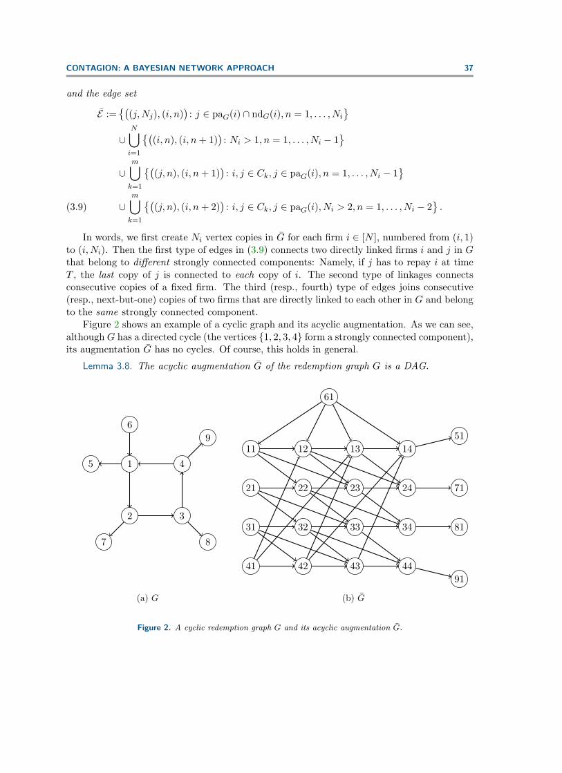
In words, we first create Ni vertex copies in G for each firm i ∈ [N ], numbered from (i, 1)to (i,Ni). Then the first type of edges in (3.9) connects two directly linked firms i and j in Gthat belong to different strongly connected components: Namely, if j has to repay i at timeT , the last copy of j is connected to each copy of i. The second type of linkages connectsconsecutive copies of a fixed firm. The third (resp., fourth) type of edges joins consecutive(resp., next-but-one) copies of two firms that are directly linked to each other in G and belongto the same strongly connected component.

Figure 2 shows an example of a cyclic graph and its acyclic augmentation. As we can see,although G has a directed cycle (the vertices {1, 2, 3, 4} form a strongly connected component),its augmentation G has no cycles. Of course, this holds in general.

Lemma 3.8. The acyclic augmentation G of the redemption graph G is a DAG.

1 4

2 3

5

6

7

9

8

(a) G

11 12 13 14

21 22 23 24

31 32 33 34

41 42 43 44

61

71

51

81

91

(b) G

Figure 2. A cyclic redemption graph G and its acyclic augmentation G.


Next we associate random variables to the vertices of G, in such a way that they containour variables of interest D1, . . . , DN as subsets and form a Bayesian network on G. We firstassume the mild default rule; for the strict default rule, all definitions and results are analogousand will be provided afterwards.

Definition 3.9. Let Ni be as in Definition 3.7. For i ∈ [N ] and n ∈ [Ni], we define Di0 := 0and then inductively Din = 1 if

Xi(T ) + er0TKi +∑

j∈paG(i)∩ndG(i)

erijTLij1{DjNj=0} +

∑j∈paG(i)∩deG(i)

erijTLij1{Dj,n−1=0}

− er′0TFi −

N∑j=1

erjiTLji < 0

(3.10)

and Din = 0 otherwise.

To paraphrase, we first order the strongly connected components of G in such a waythat firms in a given component have no borrowings from firms in previous components.Then, starting with those components that have no borrowings from any other component,we assign the value 1 to Din exactly when firm i defaults assuming it only receives paymentsfrom surviving firms of previous strongly connected components and from firms j in the samecomponent that have not defaulted up to the (n− 1)st step, that is, where Dj,n−1 = 0.

Theorem 3.10. Under the mild default rule the following statements are valid.(1) For all i ∈ [N ] and n ∈ [Ni] we have Di,n−1 ≤ Din and Di = DiNi.(2) The random variables {Din : i ∈ [N ], n ∈ [Ni]} form a Bayesian network on G with

conditional probabilities given by

P[Di1 = 1 | paG(Di1)] = Φ(i,Σmi1, T ),

P[Din = 1 | paG(Din)] =

1 if Di,n−1 = 1,Φ(i,Σm

in,T )−Φ(i,Σmi,n−1,T )

1−Φ(i,Σmi,n−1,T ) if Di,n−1 = 0,

n = 2, . . . , Ni,

(3.11)

where

Σmin := {j ∈ paG(i)∩ndG(i) : DjNj = 0}∪{j ∈ paG(i)∩deG(i) : Dj,n−1 = 0}, n ∈ [Ni].

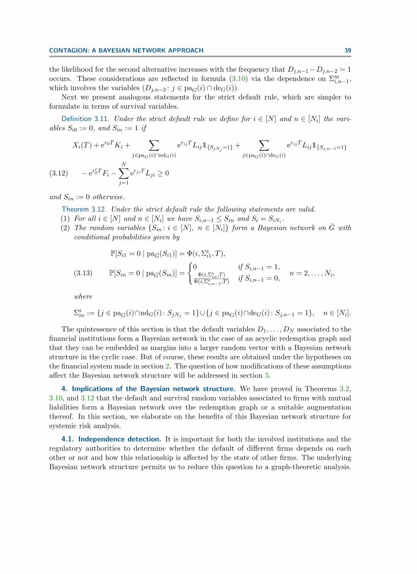
Although the variable Din does not explicitly depend on Di,n−2 in Definition 3.9, we haveto form the next-but-one edges in G (i.e., the last of the four types of edges in (3.9)). Thereason behind is that on the event Di,n−1 = 0, the values Dj,n−2 of parents j belonging tothe same strongly connected component as i contain important information about Xi(T ). Forexample, if Dj,n−2 = 1 for many such parents (so i survives in round n− 1 even though manyof its parents have defaulted in round n−2), the value Xi(T ) has to exceed a higher thresholdcompared to a situation where Dj,n−2 = 0 for many j. Furthermore, the differences Dj,n−1 −Dj,n−2 influence the likelihood of whether Di,n−1 =Din = 0 or 0 =Di,n−1 < Din = 1. In fact, ifDj,n−1−Dj,n−2 = 0 for all parents j, then necessarily the first alternative occurs. By contrast,


the likelihood for the second alternative increases with the frequency that Dj,n−1−Dj,n−2 = 1occurs. These considerations are reflected in formula (3.10) via the dependence on Σm

i,n−1,which involves the variables (Dj,n−2 : j ∈ paG(i) ∩ deG(i)).

Next we present analogous statements for the strict default rule, which are simpler toformulate in terms of survival variables.

Definition 3.11. Under the strict default rule we define for i ∈ [N ] and n ∈ [Ni] the vari-ables Si0 := 0, and Sin := 1 if

Xi(T ) + er0TKi +∑

j∈paG(i)∩ndG(i)

erijTLij1{SjNj=1} +


erijTLij1{Sj,n−1=1}

− er′0TFi −

N∑j=1

erjiTLji ≥ 0(3.12)

and Sin := 0 otherwise.

Theorem 3.12. Under the strict default rule the following statements are valid.(1) For all i ∈ [N ] and n ∈ [Ni] we have Si,n−1 ≤ Sin and Si = SiNi.(2) The random variables {Sin : i ∈ [N ], n ∈ [Ni]} form a Bayesian network on G with

conditional probabilities given by

P[Si1 = 0 | paG(Si1)] = Φ(i,Σsi1, T ),

P[Sin = 0 | paG(Sin)] =

{0 if Si,n−1 = 1,

Φ(i,Σsin,T )

Φ(i,Σsi,n−1,T ) if Si,n−1 = 0,

n = 2, . . . , Ni,(3.13)

where

Σsin := {j ∈ paG(i)∩ndG(i) : SjNj = 1}∪{j ∈ paG(i)∩deG(i) : Sj,n−1 = 1}, n ∈ [Ni].

The quintessence of this section is that the default variables D1, . . . , DN associated to thefinancial institutions form a Bayesian network in the case of an acyclic redemption graph andthat they can be embedded as margins into a larger random vector with a Bayesian networkstructure in the cyclic case. But of course, these results are obtained under the hypotheses onthe financial system made in section 2. The question of how modifications of these assumptionsaffect the Bayesian network structure will be addressed in section 5.

4. Implications of the Bayesian network structure. We have proved in Theorems 3.2,3.10, and 3.12 that the default and survival random variables associated to firms with mutualliabilities form a Bayesian network over the redemption graph or a suitable augmentationthereof. In this section, we elaborate on the benefits of this Bayesian network structure forsystemic risk analysis.

4.1. Independence detection. It is important for both the involved institutions and theregulatory authorities to determine whether the default of different firms depends on eachother or not and how this relationship is affected by the state of other firms. The underlyingBayesian network structure permits us to reduce this question to a graph-theoretic analysis.


More precisely, given the evidence of Dk, k ∈ K, for some subset K ⊆ [N ], one can determineby sole inspection of G, the augmentation of the redemption graph G from Definition 3.7,whether {Di : i ∈ I} and {Dj : j ∈ J} for two further subsets I, J ⊆ [N ] depend on each otheror not.

The key concept here is called d-separation, see p. 48 in Lauritzen (1996):

Definition 4.1. Let G = (V, E) be a graph.(1) We call i1 G · · · G in a chain between i1 and in if for every j ∈ [n − 1] we have

ij →G ij+1 or ij+1 →G ij (or both).(2) For three pairwise disjoint subsets V0, V1, V2 of V, the sets V1 and V2 are called d-

separated in G given V0 (or simply d-separated if V0 = ∅) if every chain i1 G

· · ·G in in G from some i1 ∈ V1 to some in ∈ V2 is blocked by V0; that is, for somej = 2, . . . , n− 1 we have

• ij−1 →G ij →G ij+1 and ij ∈ V0 ( type I structure), or• ij−1 ←G ij ←G ij+1 and ij ∈ V0 ( type II structure), or• ij−1 ←G ij →G ij+1 and ij ∈ V0 ( type III structure), or• ij−1 →G ij ←G ij+1 and ij /∈ V0 and deG(ij) ∩ V0 = ∅ ( type IV structure).

For example, if G is a DAG, then for every i ∈ V the sets {i} and ndG(i) are d-separatedin G given paG(i). If random variables {Xi : i ∈ V} form a Bayesian network on G, thefundamental result is the following (see Corollary 3.23 together with Proposition 3.25 inLauritzen (1996)): If V1 and V2 are d-separated in G given V0, then the two collectionsof random variables {Xi : i ∈ V1} and {Xi : i ∈ V2} are conditionally independent given{Xi : i ∈ V0}. Numerical algorithms for checking d-separation are well established and efficient(see section 3.3 of Koller and Friedman (2009)).

Applied to the acyclic augmentation G = (V, E) of the redemption graph, the d-separationcriterion provides a graphical tool for detecting independence between different groups of firmsregarding their default behavior. In fact, d-separation is “almost” necessary for independence(see Theorem 7 of Meek (1995)): If V0, V1, and V2 are subsets of V, and V1 and V2 arenot d-separated given V0, then for almost all volatility parameters σi the random variables{Di : i ∈ V1} and {Di : i ∈ V2} are stochastically dependent given {Di : i ∈ V0} if none of thevariables Di, i ∈ V1 ∪ V2, becomes deterministic given {Di : i ∈ V0}. The next propositionrelates d-separation in G to d-separation in G.

Proposition 4.2. Let G be the redemption graph and G its acyclic augmentation. Then thefollowing assertions hold for all pairwise disjoints subsets V1, V2, and V3 of [N ].

(1) V1 and V2 are d-separated in G if and only if {(i,Ni) : i ∈ V1} and {(i,Ni) : i ∈ V2}are d-separated in G.

(2) If V1 and V2 are d-separated in G given V0, then {(i, n) : i ∈ V1, n ∈ [Ni]} and{(i, n) : i ∈ V2, n ∈ [Ni]} are d-separated in G given {(i, n) : i ∈ V0, n ∈ [Ni]}.

4.2. Measures of systemic impact. In the systemic risk literature several measures ofsystemic importance for interconnected firms have been proposed. While some approacheslike in Acemoglu, Ozdaglar, and Tahbaz-Salehi (2015), Battiston et al. (2012), and Dieboldand Yilmaz (2014) are purely based on the underlying network structure and parameters,others explicitly take the probabilistic nature of contagion into account. Examples for the


latter category include the contagion index of Cont, Moussa, and Santos (2013), the CoVaRmeasure of Adrian and Brunnermeier (2016), the SES and SRISK measures of Acharya et al.(2016) and Brownlees and Engle (2017), and the general systemic risk measures of Biaginiet al. (to appear) and Feinstein, Rudloff, and Weber (2017). Based on the structural cascademodel analyzed in sections 2 and 3, we contribute two further probabilisitic measures ofsystemic risk that are flexible (one can measure the impact of a single firm or a group of firms,unconditionally or conditionally on different stress scenarios), feasible (they can be computedby the methods described in the next subsection), and robust (they depend continuously onthe underlying model parameters).

In the following, if not otherwise stated, any consistent extension of (2.2) and (2.3) canbe considered, in particular both the mild and the strict default rule.

Definition 4.3. For two disjoint subsets I and J of [N ], the absolute and the relativesystemic impact (ASI and RSI) of I on J are defined as (we use 1 to denote a vector with allentries equal to one)

ASI(I, J) := maxJ0⊆J, e∈{0,1}|J0|

(P[DJ0 = e | DI = 1]− P[DJ0 = e]

)(4.1)

and RSI(I, J) := maxe∈{0,1}|J|

log2P[DJ = e | DI = 1]

P[DJ = e](4.2)

respectively. In (4.2), we set log2 0 = −∞, and 0/0 = 1 in case the denominator, and, as aconsequence, also the numerator is zero.

The ASI of I on J equals the total variation distance between the distribution of DJ

and its conditional distribution given DI = 1. Moreover, the RSI of I on J is the Renyidivergence of order +∞ between the same pair of distributions. Of course, instead of takingthe maximum in (4.1) and (4.2), also Lp-type measures can be investigated. For example,one can define L1-analogues of the ASI and the RSI measures based on mutual informationand the Kullback–Leibler divergence. We do not go into details at this point but only referto van Erven and Harremoes (2014) for more information on distances between probabilitymeasures.

Turning to the literature on Bayesian networks, we found, to our surprise, only little re-search where measures of importance for vertices in a network are investigated. Most notably,in Chapter 4 of Pinto (1986) (cf. Pearl (1988), Chapter 6.4), the author proposes quantifyingthe relevance of a vertex Y for another vertex X by a function depending on the distributionof X and its conditional distribution given Y . They give a version of the ASI measure as anexample. Furthermore, Chan and Darwiche (2005) employ a symmetric version of the RSImeasure in the context of sensitivity analysis for Bayesian networks.

Next, we collect some basic properties of the ASI and RSI measures.

Proposition 4.4. The following assertions hold for disjoint sets I, J ⊆ [N ].(1) ASI(I, J) ∈ [0, 1) and RSI(I, J) ∈ [0,∞).(2) If J1 ⊆ J , then ASI(I, J1) ≤ ASI(I, J) and RSI(I, J1) ≤ RSI(I, J).


1

2

4

3

5

$20

$10

$10

$15

$15

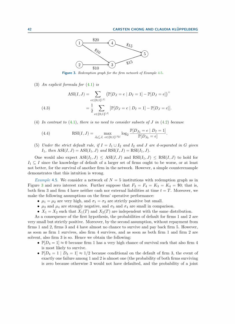
Figure 3. Redemption graph for the firm network of Example 4.5.

(3) An explicit formula for (4.1) is

ASI(I, J) =∑

e∈{0,1}|J|

(P[DJ = e | DI = 1]− P[DJ = e]

)+=

12

∑e∈{0,1}|J|

∣∣P[DJ = e | DI = 1]− P[DJ = e]∣∣.(4.3)

(4) In contrast to (4.1), there is no need to consider subsets of J in (4.2) because

(4.4) RSI(I, J) = maxJ0⊆J, e∈{0,1}|J0|

log2P[DJ0 = e | DI = 1]

P[DJ0 = e].

(5) Under the strict default rule, if I = I1 ∪ I2 and I2 and J are d-separated in G givenI1, then ASI(I, J) = ASI(I1, J) and RSI(I, J) = RSI(I1, J).

One would also expect ASI(I1, J) ≤ ASI(I, J) and RSI(I1, J) ≤ RSI(I, J) to hold forI1 ⊆ I since the knowledge of default of a larger set of firms ought to be worse, or at leastnot better, for the survival of another firm in the network. However, a simple counterexampledemonstrates that this intuition is wrong.

Example 4.5. We consider a network of N = 5 institutions with redemption graph as inFigure 3 and zero interest rates. Further suppose that F3 = F4 = K3 = K4 = $0; that is,both firm 3 and firm 4 have neither cash nor external liabilities at time t = T . Moreover, wemake the following assumptions on the firms’ operative performance:

• µ1 = µ2 are very high, and σ1 = σ2 are strictly positive but small.• µ3 and µ4 are strongly negative, and σ3 and σ4 are small in comparison.• X1 = X2 such that X1(T ) and X2(T ) are independent with the same distribution.

As a consequence of the first hypothesis, the probabilities of default for firms 1 and 2 arevery small but strictly positive. Moreover, by the second assumption, without repayment fromfirms 1 and 2, firms 3 and 4 have almost no chance to survive and pay back firm 5. However,as soon as firm 1 survives, also firm 4 survives, and as soon as both firm 1 and firm 2 aresolvent, also firm 3 is so. Hence we obtain the following:

• P[D4 = 1] ≈ 0 because firm 1 has a very high chance of survival such that also firm 4is most likely to survive.• P[D4 = 1 | D3 = 1] ≈ 1/2 because conditional on the default of firm 3, the event of

exactly one failure among 1 and 2 is almost one (the probability of both firms survivingis zero because otherwise 3 would not have defaulted, and the probability of a joint


default of 1 and 2 is still comparatively small). Since only the failure of firm 1 triggersthe default of 4, and X1(T ) and X2(T ) are identically distributed, the conditionaldefault probability of 4 given the default of 3 is around 1/2.• P[D4 = 1 | D2 = D3 = 1] ≈ 0 because the failure of 2 already explains the failure of 3,

so the latter gives us almost no additional information about 1 (and therefore 4).As a result, ASI({2, 3}, {4}) ≤ ASI({3}, {4}) and RSI({2, 3}, {4}) ≤ RSI({3}, {4}).

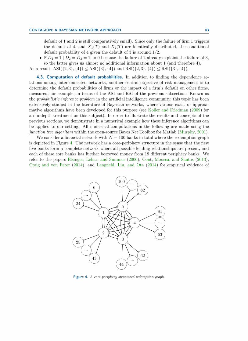
4.3. Computation of default probabilities. In addition to finding the dependence re-lations among interconnected networks, another central objective of risk management is todetermine the default probabilities of firms or the impact of a firm’s default on other firms,measured, for example, in terms of the ASI and RSI of the previous subsection. Known asthe probabilistic inference problem in the artificial intelligence community, this topic has beenextensively studied in the literature of Bayesian networks, where various exact or approxi-mative algorithms have been developed for this purpose (see Koller and Friedman (2009) foran in-depth treatment on this subject). In order to illustrate the results and concepts of theprevious sections, we demonstrate in a numerical example how these inference algorithms canbe applied to our setting. All numerical computations in the following are made using thejunction tree algorithm within the open-source Bayes Net Toolbox for Matlab (Murphy, 2001).

We consider a financial network with N = 100 banks in total where the redemption graphis depicted in Figure 4. The network has a core-periphery structure in the sense that the firstfive banks form a complete network where all possible lending relationships are present, andeach of these core banks has further borrowed money from 19 different periphery banks. Werefer to the papers Elsinger, Lehar, and Summer (2006), Cont, Moussa, and Santos (2013),Craig and von Peter (2014), and Langfield, Liu, and Ota (2014) for empirical evidence of

4

51

23

...

...

...44

62

...100

82

...

24

6

25

43

63

81

Figure 4. A core-periphery structured redemption graph.


Figure 5. Default probabilities under the mild default rule (solid line) and the strict default rule (dashed line).

such structures in real banking networks. The time horizon in our example is T = 1 year, allinterest rates are zero, and we assume statistical equality among all core banks and among allperiphery banks:

µC = 0.1, σC = 0.2, XC = 2000, FC = 500, LCC = 1600/(N − 1) = 400,µP = 0.05, σP = 0.1, XP = 80, FP = 90, LPC = 35 (if C→ P).

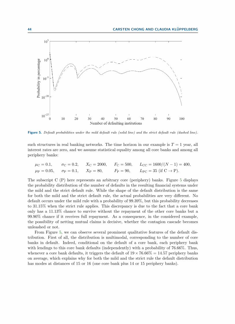
The subscript C (P) here represents an arbitrary core (periphery) banks. Figure 5 displaysthe probability distribution of the number of defaults in the resulting financial systems underthe mild and the strict default rule. While the shape of the default distribution is the samefor both the mild and the strict default rule, the actual probabilities are very different. Nodefault occurs under the mild rule with a probability of 99.39%, but this probability decreasesto 31.15% when the strict rule applies. This discrepancy is due to the fact that a core bankonly has a 11.13% chance to survive without the repayment of the other core banks but a99.90% chance if it receives full repayment. As a consequence, in the considered example,the possibility of netting mutual claims is decisive, whether the contagion cascade becomesunleashed or not.

From Figure 5, we can observe several prominent qualitative features of the default dis-tribution. First of all, the distribution is multimodal, corresponding to the number of corebanks in default. Indeed, conditional on the default of a core bank, each periphery bankwith lendings to this core bank defaults (independently) with a probability of 76.66%. Thus,whenever a core bank defaults, it triggers the default of 19× 76.66% = 14.57 periphery bankson average, which explains why for both the mild and the strict rule the default distributionhas modes at distances of 15 or 16 (one core bank plus 14 or 15 periphery banks).


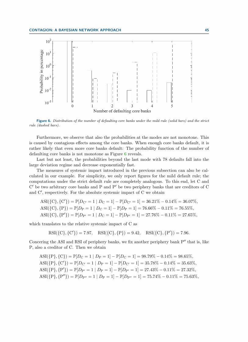
Figure 6. Distribution of the number of defaulting core banks under the mild rule (solid bars) and the strictrule (dashed bars).

Furthermore, we observe that also the probabilities at the modes are not monotone. Thisis caused by contagious effects among the core banks. When enough core banks default, it israther likely that even more core banks default: The probability function of the number ofdefaulting core banks is not monotone as Figure 6 reveals.

Last but not least, the probabilities beyond the last mode with 78 defaults fall into thelarge deviation regime and decrease exponentially fast.

The measures of systemic impact introduced in the previous subsection can also be cal-culated in our example. For simplicity, we only report figures for the mild default rule; thecomputations under the strict default rule are completely analogous. To this end, let C andC′ be two arbitrary core banks and P and P′ be two periphery banks that are creditors of Cand C′, respectively. For the absolute systemic impact of C we obtain

ASI({C}, {C′}) = P[DC′ = 1 | DC = 1]− P[DC′ = 1] = 36.21%− 0.14% = 36.07%,ASI({C}, {P}) = P[DP = 1 | DC = 1]− P[DP = 1] = 76.66%− 0.11% = 76.55%,ASI({C}, {P′}) = P[DP′ = 1 | DC = 1]− P[DP′ = 1] = 27.76%− 0.11% = 27.65%,

which translates to the relative systemic impact of C as

RSI({C}, {C′}) = 7.97, RSI({C}, {P}) = 9.42, RSI({C}, {P′}) = 7.96.

Concering the ASI and RSI of periphery banks, we fix another periphery bank P′′ that is, likeP, also a creditor of C. Then we obtain

ASI({P}, {C}) = P[DC = 1 | DP = 1]− P[DC = 1] = 98.79%− 0.14% = 98.65%,ASI({P}, {C′}) = P[DC′ = 1 | DP = 1]− P[DC′ = 1] = 35.78%− 0.14% = 35.63%,ASI({P}, {P′}) = P[DP′ = 1 | DP = 1]− P[DP′ = 1] = 27.43%− 0.11% = 27.32%,ASI({P}, {P′′}) = P[DP′′ = 1 | DP = 1]− P[DP′′ = 1] = 75.74%− 0.11% = 75.63%,


and

RSI({P}, {C}) = 9.42, RSI({P}, {C′}) = 7.96, RSI({P}, {P′}) = 7.94,RSI({P}, {P′′}) = 9.40.

As both the ASI and RSI reveal, even banks that are not direct counterparties may besystemically important for each other. For instance, if a core bank defaults, the defaultprobability of a periphery bank increases by 27.65% (or by a factor of 27.96 ≈ 248) even ifit has no lendings to that defaulted core bank. Another observation is that also peripherybanks have a high systemic impact although they have no borrowings from other banks in thesystem. The reason behind is simply that periphery banks that are repaid by their core bankcounterparty survive with a probability larger than 99.99%. So if a periphery bank defaults,this is very likely caused by the default of its core bank counterparty.

5. Conclusion and outlook. In this paper we analyzed a financial contagion model inwhich the joint default probability distribution of the system can be characterized in terms ofa Bayesian network on a graph determined by the interfirm liabilities. We further explainedhow this graphical structure can be employed to detect systemic dependencies within thenetwork, to define measures of systemic importance for institutions, and to compute theirconditional or unconditional default probabilities. Since the involved methodologies apply toall possible networks, this work provides a useful device to analyze and monitor the systemicrisk in financial systems.

Naturally, we did impose various conditions on the financial network, so let us commenton possible generalizations. First of all, regarding probabilistic assumptions, the lognormalhypothesis on the evolution of the operating firm assets is merely for simplicity. The Bayesiannetwork structure of the default variables is preserved if we assume another distribution forthe asset returns. Only the conditional probabilities stated in Theorems 3.2, 3.10, and 3.12have to be adapted.

The situation is different if we allow for dependent asset returns of the financial institu-tions. Of course, if one is only interested in computing default probabilities using Monte Carlotechniques, this is still feasible as long as the joint asset return distribution can be simulatedfrom. However, the Bayesian network structure of the default variables D1, . . . , DN will be lostin general because observations of nondescendant institutions (with respect to the redemptiongraph) may reveal additional information about the driving noise. But let us suppose thateach institution i is driven by a finite number of common market noises W1, . . . ,WK plus itsown idiosyncratic noise Bi, assuming that the Bi’s are still independent and also independentof the Wj ’s. Then conditional on the Wj ’s, the variables D1, . . . , DN will have a Bayesiannetwork structure. Hence, our approach permits default risk analysis under various marketsituations, which is useful for stress testing, for instance.

Other generalizations may concern the assumptions on the financial system itself andthe way institutions are interconnected. In our model, all mutual exposures are loans withtwo possible values at the end of the period (depending on whether the counterparty fails ornot). It would be more realistic to include other types of exposures, for example, exposureswith continuously varying values like asset cross-holdings (cf. Gourieroux, Heam, and Monfort(2012) and Elliott, Golub, and Jackson (2014)), exposures with different seniorities, exposures


with a nonzero recovery rate in the case of counterparty default, or exposures with differentmaturity dates. These considerations clearly go beyond the scope of the current paper andare left to future research.

Appendix A. Proofs.

Proof of Theorem 2.4. (1) If G is a DAG, the relation .G defined in (3.7) induces apartial order on {1, . . . , N} with a nonempty set V1 of minimal nodes with respect to .G,which precisely contains those firms that have not lent money to any other firm. For sucha firm i ∈ V1, the equation for Ei(T ) in (2.3) is explicit: It does not depend on any otherj 6= i because Lij = 0. Next, we consider the minimal nodes in V \V1 with respect to .GV\V1

,that is, those firms that have only lent money to firms in V1. Their values Ei(T ) are given byan expression involving Ej(T ) only for j ∈ V1. Iterating this at most N times, we obtain anexplicit formula for all Ei(T ) in terms of X1(T ), . . . , XN (T ) and the model parameters.

(2) Now we suppose that G has a directed cycle, say, involving the firms 1, . . . , N0 inthat order. By assumption (2.1), for each firm i ∈ {N0 + 1, . . . , N} there exists a range[x(1)i , x

(2)i ) with 0 = x

(1)i < x

(2)i such that i necessarily defaults whenever Xi(T ) falls into this

interval. For the N0 firms within the cycle we first define L0 to be the smallest amount a firmin {1, . . . , N0} has to repay to its creditor within the cycle. An inspection of (2.3) revealsthat there exists a rectangle

∏N0i=1[x(1)

i , x(2)i ) with x

(1)i < x

(2)i and the following property:

When (X1(T ), . . . , XN0(T )) lies in that rectangle, then each firm in [N0] is able to repaythe external liabilities and all its creditors except the one in the cycle, but the remainingasset value is larger than the debt owed to this cycle creditor minus L0. As a result, if(X1(T ), . . . , XN (T )) ∈

∏Ni=1[x(1)

i , x(2)i ), which is an event with strictly positive probability,

then one solution would be that all firms default, and another would be that the firms in thecycle survive while all other firms default.

Proof of Theorem 3.2. This theorem is a special case of Theorem 3.12.

Proof of Proposition 3.3. That (3.6) holds with “≤” is immediate: If S = Σ, equation(2.3) becomes an explicit expression in terms of Xi(T ) and the model parameters for eachi ∈ [N ]. The independence of X1(T ), . . . , XN (T ) together with their lognormal distributionsyields (3.6) with “≤.” In order to prove equality when both GΣ and G[N ]\Σ are DAGs, weconsider the situation where X1(T ), . . . , XN (T ) satisfy (2.2) and (2.3) with S = Σ. We haveto show that all other choices S = Σ′ with Σ′ 6= Σ would violate (2.2) and (2.3). Since GΣ isa DAG, the relation .GΣ induces a partial order on Σ. The minimal nodes in Σ with respectto that partial order, denoted by Σ1, correspond to firms that survive without receiving anypayment from other firms in the network at time T . So they must belong to Σ′ wheneverS = Σ′ is supposed to satisfy (2.2) and (2.3). Next, we consider the minimal nodes in Σ \Σ1.Again, they must belong to Σ′ because they survive regardless of the solvency of all other firmsexcept for the minimal nodes, which, however, are already known to survive. Inductively, thisproves that Σ ⊆ Σ′ for every potential Σ′. Similarly, because G[N ]\Σ is a DAG, the maximalelements in [N ] \ Σ default regardless of whether the other firms in [N ] \ Σ default or not,so they cannot belong to Σ′. An analogous induction argument yields [N ] \ Σ ⊆ [N ] \ Σ′, soΣ = Σ′.


Proof of Proposition 3.6. We assume the strict default rule; for the mild default rule, theproof is completely analogous.

(1) It is obvious that the strict default rule maps X1(T ), . . . , XN (T ) in a measurable wayto S1, . . . , SN . So we are left to prove that for i ∈ [N ] the term in (2.3) is nonnegative if andonly if i ∈ S. By Definition 3.5, the expression (2.3) for i ∈ Sn is already nonnegative whenwe take the indicator 1Sn−1 (for n = 1 we set S0 := ∅), which is always less than or equal tothe original indicator 1S . Since S = S1 ∪ · · · ∪ SN , this proves that (2.3) is nonnegative forall i ∈ S. By contrast, for all i ∈ D equation (2.3) must take a strictly negative value becauseotherwise i belongs to S1 ∪ · · · ∪ SN0+1 according to the strict default rule where N0 is thesmallest number in [N ] such that S = S1 ∪ · · · ∪ SN0 , which is obviously a contradiction.

(2) Denote by S1, . . . ,SN the surviving firms of the nth round under the strict defaultrule. As in (1), a simple induction argument shows that Sn ⊆ S holds for all n ∈ [N ] wheneverS and D satisfy (2.2) and (2.3).

(3) We have already shown in Proposition 3.3 that (3.6) always holds with “≤.” For thereverse inequality, suppose that X1(T ), . . . , XN (T ) satisfy (2.2) and (2.3) with Σ instead ofS. Under the strict default rule, the proof of the same proposition reveals that, because ofthe DAG structure of GΣ, we necessarily have Σ ⊆ S, so part (2) of the current propositioncompletes the proof.

Proof of Lemma 3.8. Suppose that G does have a cycle, say, of the form

(i1, n1)→G · · · →G (ik, nk)→G (i1, n1).

Then at least one of the edges must belong to the first of the four collections of edges in (3.9)because otherwise we would have n1 < n2 < · · · < nk < n1, which is absurd. But if the cyclehas an edge of the form ((il, Nil), (il+1, nl+1)) with il ∈ paG(il+1) ∩ ndG(il+1), there cannotexist a path in G that connects (il+1, nl+1) to (il, Nil) because, by (3.9), this would give rise toa path in G from il+1 to il and contradict the fact that il ∈ ndG(il+1). However, this in turnproduces a contradiction to the assumption that (i1, n1), . . . , (ik, nk) form a cycle in G.

Proof of Theorem 3.10. (1) The first statement follows immediately from the definitionin (3.10). For the second statement we number the strongly connected components of G insuch a way that no vertex in Ck has parents in Ck+1, . . . , Cm. By induction on k we mayassume that Di = DiNi holds under the mild default rule for all i ∈ C1 ∪ · · · ∪ Ck−1. Wemust prove that Di = DiNi is true for i ∈ Ck. We first show that Di = 1 holds as soon asDin = 1 for some n ∈ [Ni]. To this end, we proceed with another induction on n and assumethat we already know that Dj,n−1 = 1 implies Dj = 1 for all j ∈ Ck. Then firms i ∈ Ck withDin = 1 cannot repay their debts if they only receive payments from j ∈ paG(i) \ Ck withDjNj = 0 and j ∈ paG(i) ∩ Ck with Dj,n−1 = 0. Indeed, all other firms default under themild default rule: Firms j ∈ paG(i) \Ck with DjNj = 1 by the first induction hypothesis andfirms j ∈ paG(i) ∩ Ck with Dj,n−1 = 1 by the second. Thus, also i must default according tothe mild default rule. For the converse direction that Di = 1 implies DiNi = 1 for all i ∈ Ck,we recall that D =

⋃Nn=1Dn, where Dn contains the defaulting firms of the nth round. By

induction on n ∈ [N ], let us assume that those i ∈ Ck that belong to D1 ∪ · · · ∪ Dn−1 satisfyDiNi = 1. Then every i ∈ Dn has a negative equity value at time T if it does not receivemoney back from j ∈ paG(i) ∩ (D1 ∪ · · · ∪ Dn−1). If such a firm j belongs to paG(i) \ Ck,


we have DjNj = 1 by the first induction hypothesis, while if it belongs to paG(i) ∩ Ck, wehave DjNj = 1 by the second hypothesis, and consequently Dj,Nj−1 = 1 (because the eventthat Dj,Nj−1 = 0 and DjNj = 1 happens only if j defaults in a later round than all firms inCk, which, however, is not possible because j ∈ D1 ∪ · · · ∪ Dn−1 and i ∈ Dn). Therefore, weconclude that DiNi = 1, which ends the proof of Di = DiNi for i ∈ Ck.

(2) If {ein : i ∈ [N ], n ∈ [Ni]} is a given sequence taking values 0 or 1, then, because of(1), the probability that Din = ein for all i and n can only be larger than zero if ein ≤ ei,n+1for all i ∈ [N ] with Ni > 1 and n ∈ [Ni − 1]. In this case, we define for i ∈ [N ] the number

ni :=

{min{n ∈ [Ni] : ein = 1} if eiNi = 1Ni + 1 if eiNi = 0

and observe that Din = ein holds for all i ∈ [N ] and n ∈ [Ni] if and only if (with ei0 := 0 andthe abbreviation Li(T ) := er

′0TFi +

∑Nj=1 erjiTLji − er0TKi)

• for all i ∈ [N ] with ni = 1 we have

Xi(T ) < Li(T )−∑

j∈paG(i)∩ndG(i)

erijTLij1{ejNj=0},

• for all i ∈ [N ] with ni = Ni + 1 we have

Xi(T ) ≥ Li(T )−∑

j∈paG(i)∩ndG(i)

erijTLij1{ejNj=0} −


erijTLij1{ej,Ni−1=0},

• and for all i ∈ [N ] with 2 ≤ ni ≤ Ni we have

Xi(T ) < Li(T )−∑

j∈paG(i)∩ndG(i)



erijTLij1{ej,ni−1=0}

and

Xi(T ) ≥ Li(T )−∑

j∈paG(i)∩ndG(i)



erijTLij1{ej,ni−2=0}.

Thus, using the independence of X1(T ), . . . , XN (T ) and their lognormal distribution, we ob-tain on the one hand

P[Din = ein ∀i ∈ [N ], n ∈ [Ni]]

=∏

i : ni=1

Φ(i, Σmini, T )

∏i : 2≤ni≤Ni

(Φ(i, Σmini, T )− Φ(i, Σm

i,ni−1, T ))

×∏

i : ni=Ni+1

(1− Φ(i, Σmi,ni−1, T )),(A.1)

where Σmin := {j ∈ paG(i) ∩ ndG(i) : ejNj = 0} ∪ {j ∈ paG(i) ∩ deG(i) : ej,n−1 = 0}.


On the other hand, if we assume for a moment that formula (3.13) is valid, we deducethat for all i ∈ [N ] with ni = 1 we have

Ni∏n=1

P[Din = ein | paG(Din) = paG(ein)] = P[Di1 = 1 | paG(Din) = paG(ein)]

= Φ(i, Σmi1, T ),

that for all i ∈ [N ] with ni = Ni + 1 we have

Ni∏n=1

P[Din = ein | paG(Din) = paG(ein)] =Ni∏n=1

P[Din = 0 | paG(Din) = paG(ein)]

= (1− Φ(i, Σmi1, T ))

Ni∏n=2

1− Φ(i, Σmin, T )

1− Φ(i, Σmi,n−1, T )

= 1− Φ(i, ΣmiNi, T ),

and that for all other i ∈ [N ] with 2 ≤ ni ≤ Ni we have

Ni∏n=1

P[Din = ein | paG(Din) = paG(ein)]

= P[Dini = 1 | paG(Dini) = paG(ein)]ni−1∏n=1

P[Din = 0 | paG(Din) = paG(ein)]

=Φ(i, Σm

ini, T )− Φ(i, Σm

i,ni−1, T )1− Φ(i, Σm

i,ni−1, T )(1− Φ(i, Σm

i1, T ))ni−1∏n=2

1− Φ(i, Σmin, T )

1− Φ(i, Σmi,n−1, T )

= Φ(i, Σmini, T )− Φ(i, Σm

i,ni−1, T ).

Comparing with (A.1), we conclude that

P[Din = ein ∀i ∈ [N ], n ∈ [Ni]] =N∏i=1

Ni∏n=1

P[Din = ein | paG(Din) = paG(ein)],

which proves that the random variables {Din : i ∈ [N ], n ∈ [Ni]} form a Bayesian networkon G.

It remains to demonstrate the correctness of the conditional probabilities stated in (3.13).We only carry out the proof for Ni > 1 and n > 1; the case n = 1 is simpler and can beachieved by a straightforward modification of the following arguments. It is evident by themonotonicity statement in (1) that ei,n−1 = 1 immediately implies

P[Din = 1 | paG(Din) = paG(ein)] = 1,

so only the case ei,n−1 = ei,n−2 = · · · = ei1 = 0 needs to be considered further. Conditionalon Di,n−1 = 0, we can now represent the parents of Din as

paG(Din) = Fn(Xj(T ) : j ∈ anG(i) \ {i})


with some function Fn whose explicit form can be derived from (3.10). Thus, abbreviating

Min := Li(T )−∑

j∈paG(i)∩ndG(i)



erijTLij1{ej,n−1=0},

we obtain

P[Din = 1 | paG(Din) = paG(ein)]= P[Xi(T ) < Min | Xi(T ) ≥Mi,n−1, Fn(Xj(T ) : j ∈ anG(i) \ {i}) = paG(ein)]= P[Xi(T ) < Min | Xi(T ) ≥Mi,n−1]

by the independence of X1(T ), . . . , XN (T ). This is exactly what formula (3.11) states.

Proof of Theorem 3.12. The proof is completely analogous to that of Theorem 3.10.

Proof of Proposition 4.2. (1) We first assume that V1 and V2 are d-separated in G andpick a chain between some (i1, Ni1) and (ik, Nik) with i1 ∈ V1 and ik ∈ V2. Observing that(i, n)→G (i′, n′) implies i = i′ or i→G i

′, it follows that the chain under consideration cannotbe a path (otherwise also i1 and ik would be connected through a path in G, which contradictsd-separation). It can neither be of the form

(i1, Ni1)←G · · · ←G (ij , nj)→G · · · →G (ik, Nik),

as this would entail a chain in G of the same form, which would again violate the d-separationassumption. As a result, the chain in G must contain a type IV structure and is thereforeblocked. The other direction follows similarly, and we omit the details.

(2) Every chain (i1, n1) G · · · G (ik, nk) with i1 ∈ V1 and ik ∈ V2 induces a chaini1 G · · · G ik in G, where consecutive copies of a vertex are understood as merged to asingle vertex. By assumption, this chain in G must be blocked by V0 and therefore contain atleast one blocking structure of type I–IV. If a blocking structure of type I, II, or III is present,say, with middle vertex ij , then ij ∈ V0 and the corresponding sequence in the original chainin G must contain a structure of the same type with some middle vertex (ij , n) and somen ∈ [Nij ], hence blocking the chain in G. Similarly, for the last remaining case, if the chain inG has a blocking structure of type IV, say, again with middle node ij , then V0 contains neitherij nor any of its descendants. Since this immediately implies that {(i, n) : i ∈ V0, n ∈ [Ni]}and {(i, n) : i = ij or i ∈ deG(ij), n ∈ [Ni]} are disjoint, and the original chain in G necessarilyhas a type IV structure with some middle vertex (ij , n) and some n ∈ [Nij ], it is blocked by{(i, n) : i ∈ V0, n ∈ [Ni]}.

Proof of Proposition 4.4. (1) is obviously true. In (2) the statement for the absolute sys-temic impact follows from the definition, while it follows from (4) for the relative systemicimpact. (3) is a well-known result (see Proposition 4.2 and the following remark in Levin,Peres, and Wilmer (2009)). Next, (4) is a consequence of an elementary inequality: If a/band c/d are bounded by M , then also (a + c)/(b + d). Therefore, the maximum in (4.4) isattained on J . Finally, for (5) we notice that if I2 and J are d-separated in G given I1, then{(i,Ni) : i ∈ I2} and {(j,Nj) : j ∈ J} are d-separated in G given {(i, n) : i ∈ I1, n ∈ [Ni]}.Since observing SI1 = 0 means Sin = 0 for all i ∈ I1 and n ∈ [Ni], the claim follows from thefact that d-separation entails independence in Bayesian networks.


Acknowledgments. We are grateful to Rama Cont for enlightening discussions on systemicrisk and to the Isaac Newton Institute of the University of Cambridge for its hospitality.

REFERENCES

D. Acemoglu, A. Ozdaglar, and A. Tahbaz-Salehi (2015), Systemic risk and stability in financial net-works, Amer. Econ. Rev., 105, pp. 564–608.

V. V. Acharya, L.H. Pedersen, T. Philippon, and M. Richardson (2016), Measuring systemic risk, Rev.Financ. Stud., 30, pp. 2–47.

T. Adrian and M. K. Brunnermeier (2016), CoVaR, Amer. Econ. Rev., 106, pp. 1705–1741.F. Allen and D. Gale (2000), Financial contagion, J. Polit. Econ., 108, pp. 1–33.H. Amini, R. Cont, and A. Minca (2016), Resilience to contagion in financial networks, Math. Finance, 26,

pp. 329–365.K. Anand, B. Craig, and G. von Peter (2015), Filling in the blanks: Network structure and interbank

contagion, Quant. Finance, 15, pp. 625–636.S. Battiston, M. Puliga, R. Kaushik, P. Tasca, and G. Caldarelli (2012), DebtRank: Too central to

fail? Financial networks, the FED and systemic risk, Sci. Rep., 2, pp. 1–6.F. Biagini, J.-P. Fouque, M. Frittelli, and T. Meyer-Brandis, A unified approach to systemic risk

measures via acceptance sets, Math. Finance, to appear.C. Brownlees and R. F. Engle (2017), SRISK: A conditional capital shortfall measure of systemic risk,

Rev. Financ. Stud., 30, pp. 48–79.F. Castiglionesi and M. Eboli (2015), Liquidity Flows in Interbank Networks, preprint, at https://sites.

google.com/site/fabiocasti2310/research-1.H. Chan and A. Darwiche (2005), A distance measure for bounding probabilistic belief change, Internat. J.

Approx. Reason., 38, pp. 149–174.C. Chong and C. Kluppelberg (2017), Partial Mean Field Limits in Heterogeneous Networks, preprint,

http://arxiv.org/abs/1507.01905.R. Cont, A. Moussa, and E. B. Santos (2013), Network structure and systemic risk in banking systems,

in Handbook on Systemic Risk, J.-P. Fouque and J. A. Langsam, eds., Cambridge University Press, Cam-bridge, pp. 327–367.

B. Craig and G. von Peter (2014), Interbank tiering and money center banks, J. Financ. Intermed., 23,pp. 322–347.

N. Detering, T. Meyer-Brandis, K. Panagiotou, and D. Ritter (2017), Managing Default Contagionin Inhomogeneous Financial Networks, preprint, http://arxiv.org/abs/1610.09542.

F. X. Diebold and K. Yilmaz (2014), On the network topology of variance decompositions: Measuring theconnectedness of financial firms, J. Econom., 182, pp. 119–134.

L. Eisenberg and T. H. Noe (2001), Systemic risk in financial systems, Manag. Sci., 47, pp. 236–249.M. Elliott, B. Golub, and M. O. Jackson (2011), Financial networks and contagion, Amer. Econ. Rev.,

104, pp. 3115–3153.H. Elsinger, A. Lehar, and M. Summer (2006), Risk assessment for banking systems, Manag. Sci., 52,

pp. 1301–1314.Z. Feinstein, B. Rudloff, and S. Weber (2017), Measures of systemic risk, SIAM J. Financial Math., 8,

pp. 672–708.J.-P. Fouque and L.-H. Sun (2013), Systemic risk illustrated, in Handbook on Systemic Risk, J.-P. Fouque

and J. A. Langsam, eds., Cambridge University Press, Cambridge, pp. 444–452.X. Freixas, B. M. Parigi, and J.-C. Rochet (2000), Systemic risk, interbank relations, and liquidity pro-

vision by the central bank, J. Money Credit Bank., 32, pp. 611–638.P. Gai and S. Kapadia (2010), Contagion in financial networks, Proc. R. Soc. A, 466, pp. 2401–2423.A. Gandy and L. A. M. Veraart (2016), A Bayesian methodology for systemic risk assessment in financial

networks, Manag. Sci., 63, pp. 4428–4446.P. Glasserman and H. P. Young (2015), How likely is contagion in financial networks?, J. Bank. Finance,

50, pp. 383–399.

https://sites.google.com/site/fabiocasti2310/research-1

https://sites.google.com/site/fabiocasti2310/research-1

http://arxiv.org/abs/1507.01905

http://arxiv.org/abs/1610.09542


C. Gourieroux, J.-C. Heam, and A. Monfort (2012), Bilateral exposures and systemic solvency risk, Can.J. Econ., 45, pp. 1273–1309.

T. R. Hurd (2016), Contagion! Systemic Risk in Financial Networks, Springer, Cham.O. Kley, C. Kluppelberg, and L. Reichel (2015), Systemic risk through contagion in a core–periphery

structured banking network, in Advances in Mathematics of Finance, A. Palczewski and L. Stettner, eds.,Banach Center Publications, Warsaw, pp. 133–149.

D. Koller and N. Friedman (2009), Probabilistic Graphical Models, MIT Press, Cambridge, MA.M. Kusnetsov and L. A. M. Veraart (2016), Interbank Clearing in Financial Networks with Multiple

Maturities, preprint, https://ssrn.com/abstract=2854733.S. Langfield, Z. Liu, and T. Ota (2014), Mapping the UK interbank system, J. Bank. Finance, 45, pp.

288–303.S. L. Lauritzen (1996), Graphical Models, Clarendon Press, Oxford.D. A. Levin, Y. Peres, and E. L. Wilmer (2009), Markov Chains and Mixing Times, American Mathemat-

ical Society, Providence, RI.C. Meek (1995), Strong completeness and faithfulness in Bayesian networks, Uncertainty in Artificial In-

telligence, in Proceedings of the Eleventh Conference (1995), P. Besnard, ed., Morgan Kaufmann, SanFrancisco, CA, pp. 411–418.

C. Memmel, A. Sachs, and I. Stein (2012), Contagion in the interbank market with stochastic loss givendefault, Int. J. Cent. Bank., 8, pp. 177–206.

R. C. Merton (1974), On the pricing of corporate debt: The risk structure of interest rates, J. Finance, 29,pp. 449–470.

K. P. Murphy (2001), The Bayes Net Toolbox for MATLAB, in E. J. Wegman, A. Braverman, A. Goodman,and P. Smyth, eds., Computing Science and Statistics, vol. 33, Interface Foundation of North America,Fairfax Station, VA, pp. 331–350.

J. Pearl (1988), Probabilistic Reasoning in Intelligent Systems, Morgan Kaufmann, San Francisco, CA.J. A. Pinto (1986), Relevance Based Propagation in Bayesian Networks, Master’s thesis, University of

California, Berkeley, ftp://ftp.cs.ucla.edu/tech-report/198 -reports/860098.pdf.L. C. G. Rogers and L. A. M. Veraart (2013), Failure and rescue in an interbank network, Manag. Sci.,

59, pp. 882–898.C. Upper (2011), Simulation methods to assess the danger of contagion in interbank markets, J. Financ. Stab.,

7, pp. 111–125.T. van Erven and P. Harremoes (2014), Renyi divergence and Kullback-Leibler divergence, IEEE Trans.

Inform. Theory, 60, pp. 3797–3820.

https://ssrn.com/abstract=2854733

ftp://ftp.cs.ucla.edu/tech-report/198_-reports/860098.pdf

Documents

Contagion in Financial Systems: A Bayesian Network Approach fileSIAM J. FINANCIAL MATH. c 2018 Society for Industrial and Applied Mathematics Vol. 9, No. 1, pp. 28{53 Contagion in