Contagion as a Wealth Effect - Princeton Universitywxiong/papers/contagion.pdf · financial intermediaries to withdraw from illiquid investments. Caballero and Krishnamurthy ~2000!

Contagion as a Wealth Effect

ALBERT S. KYLE and WEI XIONG*

ABSTRACT

Financial contagion is described as a wealth effect in a continuous-time model withtwo risky assets and three types of traders. Noise traders trade randomly in onemarket. Long-term investors provide liquidity using a linear rule based on funda-mentals. Convergence traders with logarithmic utility trade optimally in both mar-kets. Asset price dynamics are endogenously determined ~numerically! as functionsof endogenous wealth and exogenous noise. When convergence traders lose money,they liquidate positions in both markets. This creates contagion, in that returnsbecome more volatile and more correlated. Contagion reduces benefits from port-folio diversification and raises issues for risk management.

DURING THE FINANCIAL PANIC ASSOCIATED with the default of the Russian govern-ment in August 1998 and the subsequent collapse of the hedge fund Long TermCapital Management, numerous hedge funds, banks, and securities firms triedsimultaneously to reduce exposures to a variety of financial instruments, suchas Russian bonds, Brazilian stocks, U.S. mortgages, spreads between on-the-run and off-the-run government securities, and spreads between swaps and U.S.Treasuries. Although the fundamental values of these positions would appearto have little correlation, during this financial crisis, the asset prices in thesemarkets exhibited the following common empirical pattern:

1. Financial intermediaries suffered losses as prices moved against theirpositions;

2. Market depth and liquidity decreased simultaneously in several markets;3. The volatility of prices increased simultaneously in several markets;

and,4. Correlation of price changes of seemingly independent positions of fi-

nancial intermediaries increased.

Instead of using the term “panic” to describe the crisis, market commen-tators blamed the market behavior on increased “risk aversion” on the partof traders who follow “short-term” trading strategies. The commentators de-

* Kyle is with Fuqua School of Business, Duke University. Xiong is with Bendheim Centerfor Finance, Princeton University. We thank seminar participants at Rice University, SydneyUniversity, Tel Aviv University, Tilburg University, University College London, University ofToulouse, Conference on Hedge Funds at Duke University in November 1999, Conference onLiquidity Risks in Frankfurt, Germany in July 2000, Eleventh Annual Conference in FinancialEconomics and Accounting in University of Michigan Business School and 2001 AFA meetingsin New Orleans for valuable discussions and comments.

THE JOURNAL OF FINANCE • VOL. LVI, NO. 4 • AUGUST 2001

1401

scribed “contagion” as the rapid spread from one market to another of de-clining prices, declining liquidity, increased volatility, and increased correlationassociated with the financial intermediaries’ own effect on the markets inwhich they trade.

The purpose of this paper is to explain contagion with a theoretical modelin which increased risk aversion is based on a wealth effect of financialintermediaries. Financial intermediaries are modeled as a group of perfectlycompetitive convergence traders who speculate that the transitory effect ofnoise trading on asset prices will induce temporary deviations of prices fromtheir long-term mean. Convergence traders trade in markets for two riskyassets. When convergence traders suffer trading losses, they have a reducedcapacity for bearing risks. This motivates them to liquidate positions in bothmarkets, resulting in reduced market liquidity, increased price volatility inboth markets, and increased correlation. Through this mechanism, the wealtheffect leads to contagion. This mechanism is consistent with the report pub-lished by Bank for International Settlements ~BIS; 1999! and empirical stud-ies of Kaminsky and Reinhart ~2000!.

This paper describes a continuous-time model in which convergence trad-ers follow short-term ~but rational! trading strategies. Two risky assets haveconstant fundamental risk measured in units of the numeraire good ~con-sumption!. Three types of investors, noise traders, long-term value-basedinvestors, and short-term convergence traders, exchange these two risky as-sets for a safe asset. Noise traders trade one of the risky assets randomly,but their position in this risky asset exhibits mean reversion. Long-terminvestors are prudent but not fully rational. They follow a robust long-terminvestment strategy holding both risky assets proportionally to the spreadbetween the asset prices and their fundamental values. This spread repre-sents the present value of trading profits to long-term investors in a worst-case scenario in which they have no opportunities to take profits early butinstead hold these assets forever, collecting all the future cash f lows. Con-vergence traders aggressively exploit short-term opportunities by taking theother side of noise trading. They are rational in the sense that they correctlytake into account the effect of all market participants on price dynamics inboth markets. Convergence traders are assumed to be perfect competitorswith logarithmic utility. Logarithmic utility implies a trading strategy inwhich both the expected trading profits and the percentage variance of theportfolio equal the short-term ~instantaneous! squared Sharpe ratio in themarket. Logarithmic utility also implies a risk management strategy thatprevents wealth from dropping to zero through dynamic portfolio rebalancing.

Xiong ~2001! develops a continuous-time equilibrium model of convergencetrading with one risky asset. Xiong shows that the convergence traders’ wealtheffect can act as an amplification mechanism that increases price volatilityand may cause convergence trading to be price destabilizing in extreme cir-cumstances. This paper shows that in an otherwise similar framework withtwo risky assets, the volatility amplification generates empirical patternswhich characterize contagion. In both Xiong ~2001! and this paper, it is as-

1402 The Journal of Finance

sumed that there is no capital inf low to the convergence-trading industrythrough entry of new convergence traders or capital inf lows to existing con-vergence traders. This assumption is consistent with Shleifer and Vishny’s~1997! argument that asymmetric information and moral hazard can causeagency problems for professional traders, therefore resulting in imperfectcapital f lows to the convergence-trading industry.

In equilibrium, the asset price dynamics and convergence traders’ wealthdynamics are simultaneously determined. This introduces endogenous risksinto our model in the sense that means and variances of asset returns areendogenous functions of two state variables: the wealth of convergence trad-ers and the positions of noise traders. There are three sources of risks: in-novations in fundamentals in each of the two markets and innovations innoise-trading supply in one market. With only two risky assets, markets areincomplete. In equilibrium, the trading strategy of a representative conver-gence trader solves a fixed-point problem. This fixed-point problem is equiv-alent to a system of two second-order partial differential equations. A numericalsolution of the equilibrium ~using a projection technique! makes it possibleto quantify, for particular parameter choices, the patterns of volatility, li-quidity, correlation, and convergence-traders’ wealth associated with contagion.

Severe “contagion” happens when noise trading deviates significantly fromits mean and convergence traders’ wealth is at some intermediate level. Inthis situation, convergence traders take large positions, and these positionsneed to be reduced in response to shocks that reduce wealth. The positionrebalancing of convergence traders leads to increased volatility in both mar-kets, increased price correlation across the two markets, and reduced mar-ket liquidity.

To understand the mechanism in convergence trading, it is useful to de-scribe the response to innovations in fundamentals separately from innova-tions in noise trading. Fundamental shocks ~in either market! cause a wealtheffect. In response to unfavorable fundamental innovations which reducewealth, convergence traders liquidate positions in a manner that tends tomagnify volatility and create correlation in the returns between the twoassets. In response to innovations in noise trading that increase the posi-tions of noise traders, two forces are at work. In addition to the wealtheffect, which motivates the convergence traders to reduce positions due toreduced wealth, they have an opposite incentive ~substitution effect! to addto positions because these positions become more profitable as noise-tradinginnovations push prices further out of line. Usually, the wealth effect is smallerthan the substitution effect and convergence traders respond to noise-trading shocks by taking the other side in a manner that reduces volatilityand adds to liquidity. In certain extreme cases, however, when convergencetraders have unusually large positions, the wealth effect dominates the sub-stitution effect and convergence traders respond to noise-trading shocks byliquidating positions. This exacerbates price volatility and consumes some ofthe liquidity provided by long-term investors. It happens exactly when con-tagion is most severe.

Contagion as a Wealth Effect 1403

In our model, the risks facing an individual convergence trader are en-dogenously determined by the trading of all market participants. The modelimplies that it is important for a risk management system to take into ac-count the additional risks such as contagion and volatility amplification cre-ated by the wealth effect of convergence traders. This view is also expressedby Morris and Shin ~2000!, who study the potential coordination failure ofmarket participants. The existence of these endogenous risks presents a chal-lenge to risk-management systems based on applying statistical tools to his-torical returns. The weaknesses of these statistical models have been discussedby Danielsson ~2000!. Our economic model, based on assumptions about theliquidity provided by long-term investors and the behavior of convergencetraders, suggests risk managers measure risks after considering the capi-talization and positions of other traders.

There is a growing literature in economics and finance studying conta-gion. Dornbusch, Park, and Claessens ~2000! provide a lengthy review. Schi-nasi and Smith ~1999! suggest that the combination of leverage and value-at-risk portfolio management rules can induce contagion, but they do notprovide an equilibrium model of the wealth effect. Gromb and Vayanos ~2000!study an equilibrium model of arbitrage trading with margin constraints,and they show a similar contagion effect to our model. The wealth effectstudied in this paper is related to the papers on portfolio insurance by Gross-man and Zhou ~1996! and Basak ~1995!. Since these models are set up incomplete markets with only market risks, they are not suitable for explain-ing contagion, the transmission of idiosyncratic risk from one small marketniche to another, for example, from Russian bond markets to U.S. mortgage-backed securities markets.

An alternative approach to our paper studies financial contagion as infor-mation transmission. The idea here is that the fundamental risks are cor-related across assets. Thus, when one asset declines in price because of noisetrading, rational traders reduce the prices of all assets if they cannot dis-tinguish declines based on fundamentals from declines based on noise trad-ing. King and Wadhwani ~1990! use this approach to explain the uniformityof price declines in world stock markets during the 1987 crash. Calvo ~1999!and Yuan ~1999! study the behavior of uninformed investors when informedtraders can be margin constrained. Since uninformed rational investors can-not distinguish between selling based on liquidity shocks and shocks to fun-damentals, they suggest that it is possible for contagion to result from confuseduninformed investors. Their studies are complementary to ours, since thewealth effect in our model operates even when asset fundamentals are un-correlated across markets.

Fleming, Kirby, and Ostdiek ~1998! find empirical evidence that cross-market hedging is associated with transmission of volatility across bond andstock markets. Kodres and Pritsker ~1998! develop a theoretical model offinancial contagion based on cross-market hedging with asymmetric infor-mation. Calvo and Mendoza ~2000! suggest that information cost and rela-tive performance compensation can induce rational herding behavior ofinvestors, thus resulting in contagion. Contagion can also be modeled as


self-fulfilling sunspot equilibrium as in Masson ~1998! and its references.Rochet and Tirole ~1996! study the propagation of financial distress throughinterbank lending. Lagunoff and Schreft ~1998! and Allen and Gale ~2000!study the fragility of financial markets through a chain reaction of banks orfinancial intermediaries to withdraw from illiquid investments. Caballeroand Krishnamurthy ~2000! show that the weakening of a country’s inter-national collateral can induce the fire sale of emerging-market assets due toimperfect international credit markets. Goldstein and Pauzner ~2000! studycontagion also as a wealth effect of investors with decreasing absolute riskaversion, but in a framework of self-fulfilling banking crisis.

On the empirical side, the implications of our model are consistent withthe following empirical regularities identified in the literature: ~1! Not allasset-price volatility is explained by fundamentals; ~2! conditional correla-tions between asset returns are not constant; and, ~3! variations in condi-tional correlations are not explained by fundamentals. The empirical literatureincludes the following: Campbell and Kyle ~1993! show that the excess vol-atility literature is consistent with the idea that noise trading increases pricevolatility. Shiller ~1989! and Pindyck and Rotemberg ~1990, 1993! find evi-dence of excess correlation in asset price comovements. Longin and Solnik~1995! find that conditional correlations of world stock markets are not con-stant. Hamao, Masulis, and Ng ~1990! and Lin, Engle, and Ito ~1994! findevidence of volatility spillover in international stock markets. Karolyi andStultz ~1996! and Connolly and Wang ~1998! find that macroeconomic an-nouncements and other public information do not affect comovements of Jap-anese and American stock markets. King, Sentana, and Wadhwani ~1994!find that observable economic variables explain only a small fraction of in-ternational stock market comovements. Balyeat and Muthuswamy ~1999!find a U-shaped relationship between correlations of stock returns and thelevel of market movement. Forbes and Rigobon ~1999! discuss the economet-ric issues of heteroskedasticity and endogeneity related to the contagion tests.Bae, Karolyi, and Stultz ~2000! use a new statistical method to measurecontagion. Ang and Chen ~2000!, Connolly and Wang ~2000!, and Longin andSolnik ~2001! find correlation to be large in market downturns.

The paper proceeds as follows. Section I introduces the structure of themodel. Section II derives the equilibrium as a fixed-point problem. Sec-tion III illustrates the equilibrium using a numerical example and discussesthe implications of the model. Section IV discusses the implications for riskmanagement. Section V concludes the paper.

The Model

The model is set up in a continuous-time framework with two risky assetsand a riskless asset. There are three types of traders: noise traders, conver-gence traders and long-term value-based investors. The two risky assets haveindependent fundamental processes. One of the assets is subject to stochas-tic and mean-reverting supply caused by noise traders. The other asset hasa fixed supply. Convergence traders are fully rational with logarithmic util-


ity and an infinite trading horizon. They trade in both assets and exploit theshort-term opportunity created by noise traders. Long-term investors holdthe assets based on the spread between the prices and the fundamentals.Long-term investors are not fully rational in the sense that they ignore theshort-term opportunity caused by noise traders, but their strategy is veryrobust to the risks of model misspecification. The trading of long-term in-vestors provides convergence traders an exit strategy during crises.

A. Asset Fundamentals

We assume that traders in the financial markets exchange a safe assetwith constant interest rate r for two risky assets, which we call asset A andasset B. In the context of convergence trading, each of these two risky assetscan be thought of as a spread position between other assets. To model howfundamental uncertainty about future cash f lows is revealed to the markets,we assume that the cash f lows of these two assets are observable, mean-reverting stochastic processes DA and DB with constant instantaneous vol-atilities sA and sB, constant rates of mean reversion lA and lB, and knownlong-term means ODA and ODB. Thus, the cash-f low processes can be written

dDA � �lA~DA � ODA !dt � sAdz A, ~1!

dDB � �lB~DB � ODB !dt � sAdz B. ~2!

We assume for simplicity that the two cash-f low processes are independent.The fundamental values PF

A and PFB of the two risky assets ~not to be con-

fused with the market prices P A and P B described later! are defined as theirexpected payoffs to a risk neutral investor discounted at the risk-free rate ofinterest ~using variations of Gordon’s growth formula!:

PFA �

ODA

r�

DA � ODA

r � lA , ~3!

PFB �

ODB

r�

DB � ODB

r � lB . ~4!

The risk-neutral returns processes dQFA and dQF

B corresponding to the fun-damental values ~not to be confused with the actual returns processes dQA

and dQB discussed later! are given by the hypothetical mark-to-market prof-its of a fully levered one-share portfolio, which collects the dividend andpays the risk-free rate of interest:

dQFA � dPF

A � ~DA � rPFA!dt, ~5!

dQFB � dPF

B � ~DB � rPFB!dt. ~6!


Using the cash-f low processes and the fundamental processes above, it isstraightforward to show that the risk neutral mark-to-market profits on as-set A and B follow Brownian motions with constant volatility, which we de-fine as sF

A and sFB:

dQFA �

sA

r � lA dz A � sFA dz A, ~7!

dQFB �

sB

r � lB dz B � sFB dz B. ~8!

The equilibrium discussed below depends on the fundamental cash-f low pro-cess only through the parameters sF

A and sFB. In other words, the specific

rates of mean reversion and the long-term means of cash f lows do not affectthe equilibrium except through their effect on sF

A and sFB. Furthermore, the

risky assets can be scaled arbitrarily ~as in a stock split! to give any level offundamental volatility, without changing the equilibrium. Thus, in what fol-lows, we assume without loss of generality that fundamental volatility is thesame for both assets and is defined by sF � sF

A � sFB.

The fact that sF is constant implies that fundamental volatility is con-stant when measured in dollars per share. Without loss of generality, we canthink of convergence trading positions as spread positions. The constant vol-atility assumption better describes the fundamental risks of typical spreadpositions. These positions have distinct long and short legs. Therefore, theydo not have natural up and down directions that justify the log-normal pro-cess associated with the concept of constant percentage volatility.

B. Market Clearing Conditions

The equilibrium prices for the two risky assets ~as opposed to the funda-mental value discussed above! arise from trading by the three different typesof market participants: long-term investors, convergence traders, and noise trad-ers. Noise traders are assumed to trade only in market A. This assumption ismade to reduce the number of state variables needed to characterize the equi-librium. Following Campbell and Kyle ~1993! and Wang ~1993!, we assume thesupply of noise traders to follow an exogenous mean-reverting process

du � �lu~u� Nu!dt � sudzu , ~9!

with Nu as the long-term mean, lu as the mean-reversion parameter, and su asthe innovation standard deviation. This process is also assumed to be inde-pendent from the fundamental cash-f low processes DA and DB. Asset B hasa fixed supply of NuB. We denote long-term investors’ demand as XL

A and XLB ,

and convergence traders’ demand as X A and X B. The market clearing con-ditions ~which hold at every point in time! can be written as

XLA � X A � u, ~10!

XLB � X B � NuB. ~11!


C. Long-term Investors

Long-term investors are assumed to have the following demand curve forthe two risky assets:

XLA �

1

kA ~PFA � P A !, ~12!

XLB �

1

kB ~PFB � P B !, ~13!

where kA � 0 and kB � 0 denote the slopes of the downward-sloping demandcurves. These demand curves are proportional to the spreads between thefundamental values and the actual prices. Graham ~1973! calls this spreada safety margin. It represents the net present value of profits to long-terminvestors when they hold the assets forever and collect all the future cashf low. This is a worst-case scenario, which happens if the safety margin doesnot change over time. If we assume long-term investors have exponentialutility and assume ~incorrectly! that the safety margin is constant over time,they would use this ~suboptimal! strategy. The slope of the demand curve isthen given by

kA � fsF2, ~14!

where f is the long-term investors’ absolute risk aversion and sF2 is the

variance of fundamental shocks.If we think of the same long-term investors as participating in both mar-

kets, then the demand in one market does not depend on prices in the otherbecause the fundamentals of the two markets are uncorrelated. Therefore,under this assumption, we should assume kA � kB because the fundamentalvolatility in the two markets is identical. However, if long-term investors aresegmented in a similar manner to Merton ~1987!, with one population oflong-term investors trading in market A and another in market B, the pa-rameters kA and kB can have different values.

According to these demand curves, long-term investors always provide li-quidity to the market. When the price falls below the fundamental value ineither market, long-term investors will buy the asset. When the price fallsfurther below the fundamental value, long-term investors will buy more.The slopes of the demand curves kA and kB measure the liquidity providedby long-term investors. Larger kA or kB mean steeper demand curves, andthus represent less liquidity from long-term investors. Notice that long-terminvestors have no wealth effects. Implicitly, they are assumed to have deeppockets ~consistent with exponential utility!. As shown later, the liquidityprovided by long-term investors provides an exit strategy for convergencetraders during crises.


While this long-term strategy is profitable, it is not optimal. Because theinventory of noise traders u changes randomly in a mean-reverting man-ner, a short-term strategy can improve the portfolio performance of long-term investors. A short-term strategy implies trading more aggressivelyagainst noise trading than the long-term strategy. This creates an oppor-tunity for convergence traders to prosper in the market by using a short-term strategy.

The rationale behind the long-term strategy is its robustness. Graham~1973! noticed a long time ago that a short-term strategy that improvesupon the long-term strategy for a given noise-trading process can be subjectto large model specification risks. Therefore, he advocates a long-term strat-egy to exploit long-term opportunities ~measured by the safety margins! inthe market. This view is consistent with recent studies on the aversion tomodel uncertainty by Epstein and Wang ~1994! and Hansen, Sargent, andTallarini ~1999!. Since the focus of our model is on the effect of convergencetraders, we simplify matters by assuming the simplistic trading rule of long-term investors.

D. Convergence Traders

Convergence traders behave optimally in response to a given noise-tradingprocess. Intuitively, this means that they make profits not only by purchas-ing risky assets when they are priced below fundamentals, but they alsomake short-term profits by taking the other side of transitory noise trading.Due to the aggressive nature of convergence trading, convergence tradersare subject to large wealth f luctuation with the leverage they may be in-duced to use. This makes their wealth effect an important variable in de-termining their asset demand. In order to capture the dependence of theirdemand on both short-term opportunity and wealth, convergence traders areassumed to be a continuum of perfect competitors who maximize an addi-tively separable logarithmic utility function with an infinite time horizonand a time-preference parameter r:

J~t! � max Et�0

`

e�rs ln~Ct�s!ds. ~15!

With logarithmic utility, convergence traders have decreasing absolute riskaversion. As their wealth gets close to zero, convergence traders become in-finitely risk averse. To prevent their wealth from becoming negative, con-vergence traders will use the liquidity provided by long-term investors toliquidate their risky positions as their wealth decreases. Note that withoutlong-term investors, there can be no equilibrium with only convergence trad-ers and noise traders, because wealth cannot be guaranteed to stay positivefor convergence traders when fundamentals have a normal distribution.

Since logarithmic utility gives convergence traders an incentive to keeptheir wealth from falling below zero, there are no bankruptcy risks, andcreditors are always willing to lend money to them at the risk-free rate r.


The trading opportunities to convergence traders are the excess returnprocesses:

dQA � dP A � ~DA � rP A !dt, ~16!

dQB � dP B � ~DB � rP B !dt, ~17!

with P A and P B denoting the prices of the risky assets ~not the fundamentalvalues PF

A and PFB!. The processes dQA and dQB represent the cash f low to

a fully levered portfolio long one share of the risky asset A or B. The con-vergence traders’ budget constraint is

dW � X AdQA � X BdQB � ~rW � C!dt, ~18!

where W denotes their wealth, C denotes their consumption, and X denotestheir demand for the risky asset in shares. Consumption C can also be in-terpreted as a dividend paid to investors in the convergence traders’ funds.The convergence traders’ demand X A, X B, and consumption C are derivedfrom their utility optimization problem.

II. The Equilibrium

This paper studies a symmetric and perfectly competitive equilibrium. Inthis equilibrium, each individual convergence trader is a price-taker, andgiven everyone else’s trading strategy, each individual convergence traderwill optimally choose the same strategy. This equilibrium condition impliesthat a representative convergence trader ’s trading strategy solves a fixed-point problem.

There are three sources of uncertainty, the fundamental shock in asset A~dz A !, the fundamental shock in asset B ~dz B !, and the noise-trading shockin asset A ~dzu!. Since there are only two risky assets, markets are incom-plete. There are also two state variables: the level of noise trading u and theaggregate wealth of convergence traders W. Due to logarithmic utility, thetotal wealth of all convergence traders can be aggregated together to repre-sent their aggregate risk-bearing capacity. Unlike models with constant ab-solute risk aversion, the exact number of convergence traders is not importantfor the equilibrium.

The fundamental variables DA and DB are not state variables. Due to thenormal distribution assumption for the cash-f low processes, the fundamen-tal risks are constant for these two assets and the dividends only measurethe levels of fundamental values. Since long-term investors trade on long-term opportunities ~safety margins! measured by the difference between theprices and fundamentals, while convergence traders trade on short-term op-portunity measured by the Sharpe ratios ~as shown later by the model!,variables DA and DB have no effects on the trading strategies of eitherlong-term investors or convergence traders. Therefore, they have no effectfor the equilibrium.


The equilibrium can be characterized by three functions: convergence trad-ers’ demand functions for the two risky assets X A~u,W ! and X B~u,W !, andconvergence traders’ consumption function C~u,W !. These three functionssolve the convergence traders’ utility optimization problem. At the same time,they always satisfy the market clearing conditions.

Given convergence traders’ demand functions X A and X B, the price func-tions of the risky assets can be derived by plugging the long-term investors’demand functions into the market clearing conditions:

P A � PFA � kA~u� X A~u,W !!, ~19!

P B � PFB � kB~ NuB � X B~u,W !!. ~20!

These equations reveal the key feature of our model that convergence trad-ers’ wealth dynamics inf luence the price dynamics of both risky assets, andcan potentially cause correlation between the two asset prices although theyare fundamentally uncorrelated. Actually, the wealth dynamics and assetprice dynamics need to be determined simultaneously in the equilibrium.

The equilibrium can be set up in three steps. In the first step, the twoexcess return processes are derived given convergence traders’ demand andconsumption functions. In the second step, convergence traders’ optimal in-vestment and consumption policies are derived given the excess return pro-cesses. Finally, the equilibrium is shown to solve a fixed-point problem thatis a system of two nonlinear second-order partial differential equations. Theseequations can be solved numerically.

A. Excess Return Processes

Given the convergence traders’ demand and consumption functions, wecan use Ito’s lemma to express the excess return processes dQA and dQB

~equations ~16! and ~17!! in terms of a drift term and innovation terms as-sociated with the three sources of uncertainty dz A, dz B, and dzu. Let mA

denote the drift and sAA , sB

A , suA denote the loadings on the innovations in

the markets. The drift and loadings on innovations are functions of the twostate variables W and u. Using analogous notation for asset B, we have

dQA � mA~u,W !dt � sAA~u,W !dz A � sB

A~u,W !dz B � suA~u,W !dzu , ~21!

dQB � mB~u,W !dt � sAB~u,W !dz A � sB

B~u,W !dz B � suB~u,W !dzu . ~22!

We can think of several of these innovation coefficients as representing con-tagion. In equation ~21!, sB

A measure the effect of an innovation in the funda-mentals of asset B on returns to asset A, that is, it captures fundamentalcontagion going from market B to market A. In equation ~22!, sA

B and suB mea-

sure the effects of innovations in fundamentals in market A and noise tradingin market A on returns in market B, that is, these terms capture fundamental


contagion and noise-trading contagion going from market A to market B. Thereis no noise-trading contagion going from market B to market A because thereis assumed to be no noise trading in market B.

The wealth effect shows up through the simultaneous relationship be-tween convergence traders’ wealth process W and the excess return pro-cesses dQA and dQB. On the one hand, shocks to the two return processeschange the aggregate wealth of convergence traders through their budgetconstraint ~equation ~18!! when they are taking positions on these two as-sets. One the other hand, the changes of convergence traders’ wealth causef luctuations in their risk-bearing capacity, and thus induce them to rebal-ance their portfolio. Their portfolio rebalancing can change the prices of thetwo assets through the market clearing conditions ~equations ~19! and ~20!!.In equilibrium, any shock to any one of these assets feeds back to itselfthrough the convergence traders’ wealth, potentially amplifying the shock.The shock will also be transmitted to the other asset through the same wealthchannel, thus resulting in a contagion effect. In this way, the wealth effectcan act as both an amplification mechanism and a contagion mechanism.

In the expressions for drifts mA, mB and innovation sensitivities sAA , sB

A ,su

A , sAB , sB

B , and suB , it is shown in Appendix A that the wealth effect appears

as a factor A~u,W ! defined by

A �1

1 � kAX AXWA � kBX BXW

B . ~23!

The subscripts u or W denote the derivatives of a function with respect tonoise trading u or wealth W, that is, XW

A is the derivative of the demand forasset A with respect to wealth. The factor A has an intuitive interpreta-tion, which is explained as follows: Let dW ' denote a hypothetical changein convergence traders’ wealth that would occur in response to an exog-enous shock ~e.g., dzD

A , dzDB , or dzu

Z! if convergence traders did not updatetheir positions in response to the changes in wealth. Let dW denote theactual change in wealth that would occur when convergence traders doupdate their positions in response to the exogenous shocks. As a result ofthe initial shock, convergence traders rebalance their portfolio by reducingtheir positions in both assets A and B by XW

A dW and XWB dW, respectively.

To induce long-term investors to pick up the positions liquidated by con-vergence traders, the prices of both assets need to drop by kAXW

A dW andkBXW

B dW. When the prices fall, the convergence traders’ wealth will fur-ther drop by X A{kAXW

A dW � X B{kBXWB dW. Therefore, an initial wealth

drop of dW ' can cause a total wealth drop of

dW � dW ' � ~kAX AXWA � kBX BXW

B !dW. ~24!

This equation gives

dW � A{dW ', ~25!


which suggests that factor A measures the magnitude of amplification causedby the wealth effect. As shown later, this amplification factor A~u,W ! is al-ways larger than 1.

It is shown in Appendix A that the coefficients of the dz terms in equations~21! and ~22! for dQA and dQB are given by

sAA � sF ~1 � kBX BXW

B !A~u,W !, ~26!

sBA � sF kAX BXW

A A~u,W !, ~27!

suA � �kAsu @~1 � Xu

A!~1 � kBX BXWB !� kBXW

A X BXuB#A~u,W !, ~28!

sAB � sF kBX AXW

B A~u,W !, ~29!

sBB � sF ~1 � kAX AXW

A !A~u,W !, ~30!

suB � kBsu @Xu

B~1 � kAX AXWA !� kAX AXW

B ~1 � XuA!#A~u,W !. ~31!

Each of these terms can be explained in an intuitive way. Let us illustratewith the first term. By using the definition of A~u,W ! in equation ~23!, theterm sA

A in equation ~26! can be rewritten as

sAA � sF @1 � kAX AXW

A A~u,W !# . ~32!

When a fundamental shock dz A hits market A, it causes an initial price changeof sF dz A and an initial wealth shock of X A{sF dz A. Through the wealth am-plification mechanism discussed above, the wealth shock will be amplified byA, resulting in a total wealth shock of X A{sF dz A{A. Convergence traders re-balance their positions in asset A by XW

A{X A{sF dz A{A. In order to clear themarket, the price of asset A needs to change further by kA{XW

A{X A{sF dz A{A toattract long-term investors to take the other side of a rebalancing trade by con-vergence traders. In this way, an initial fundamental shock of dz A can causea total price change of sF dz A @1 � kAX AXW

A A~u,W !# to asset A as indicated byequation ~32!. Similar intuitive explanations can be obtained for other vola-tility terms listed above in equations ~27! through ~31!.

The drift values mA~u,W ! and mB~u,W ! are complicated expressions involv-ing X A, X B, and derivatives to second order ~see Appendix A!. Appendix A alsogives expressions for the aggregate wealth of the convergence traders W.

B. Optimal Strategy for Convergence Traders

Given the trading opportunities to a convergence trader defined by dQA

and dQB, the value function J can be written as a function of wealth W i andthe two state variables W and u:

J~W i,u,W ! � max$X iA, X iB,C i %

Et�0

`

e�rs ln~Ct�si ! ds. ~33!


Notice that W i measures the individual convergence trader ’s wealth, whileW represents the aggregate wealth of all of convergence traders. By solvinga Bellman equation, Appendix B shows the optimal consumption and port-folio rules to be

X i A�

W i

1 � f2 � mA

~sA !2� f

mB

sAsB �, ~34!

X i B�

W i

1 � f2 � mB

~sB !2� f

mA

sAsB �, ~35!

C i � r W i. ~36!

In the formula above, mA and mB are the instantaneous risk premia of thetwo assets, sA and sB are the instantaneous volatility, and f is the instan-taneous return correlation between the two assets. All these variables arefunctions of the two state variables u and W endogenously determined by theequilibrium.

Consumption is a constant fraction of the wealth equal to the impatiencelevel r. The consumption strategy can be interpreted as a constant dividendrate. The trading strategy is also proportional to the convergence trader’swealth, because logarithmic utility implies that the convergence trader ’s riskbearing capacity is proportional to wealth. This trading strategy preventswealth from falling to zero through dynamic portfolio rebalancing. When-ever wealth drops, the convergence trader needs to liquidate some risky po-sitions across the portfolio if the trading opportunities are unchanged. Aswealth falls close to zero, the convergence trader becomes infinitely riskaverse and takes almost zero positions. The existence of long-term investorsin the market is crucial to the implementation of this strategy, because theliquidity from long-term investors provides an exit opportunity for the con-vergence traders when they need to get out of their positions.

The optimal trading strategy is short-term in the sense that it only de-pends upon the instantaneous risk premium and variance of the return pro-cesses. This contrasts with the long-term strategy used by long-term investors.This trading strategy is also myopic, that is, there is no hedging demand~against changes in the future investment opportunity set!, as discussed inMerton ~1971! and Breeden ~1979!. This is a well-known property of loga-rithmic utility, and it makes the model more tractable.

According to this optimal strategy, an individual convergence trader main-tains an instantaneously mean-variance efficient portfolio involving the tworisky assets. As shown in Appendix B, the expected trading profits in per-centage terms and the instantaneous percentage variance of the convergencetrader ’s portfolio is equal to the squared Sharpe ratio of the instantaneouslymean-variance efficient portfolio. These features highlight the importanceof Sharpe ratio for convergence traders. Also, we see the advantage of using


logarithmic utility. Logarithmic utility implies an intuitive trading strategyin terms of Sharpe ratios, similar to the way in which Sharpe ratios areactually used in markets.

C. Fixed-point Problem

In equilibrium, the portfolio and consumption rules X A~u,W !, X B~u,W !,and C~u,W ! should solve the log-utility optimization problem and satisfy themarket clearing conditions at the same time. Since optimal consumption andportfolio rules of an individual convergence trader are proportional to wealth,we can aggregate the rules of all convergence traders together by replacingthe individual wealth variable W i with aggregate wealth W. Let us denotethese aggregate optimal rules by X *A~u,W !, X *B~u,W !, and C *~u,W !. Noticethat X *A, X *B, and C * are functions of conjectured strategies X A, X B, and C,respectively, as derived explicitly in Appendix B. It is evident that this def-inition of equilibrium is equivalent to a fixed-point problem:

X *A~u,W ! � X A~u,W !, ~37!

X *B~u,W ! � X B~u,W !, ~38!

C *~u,W ! � C~u,W !. ~39!

These fixed-point conditions represent that given the portfolio and consump-tion rules of all other convergence traders, a representative convergence traderwill optimally choose the same rules. Thus, assuming a transversality con-dition holds, the calculation of equilibrium for the economy boils down tosolving a fixed-point problem.

To make the equilibrium interesting, it is assumed that convergence trad-ers’ time preference r ~also their consumption rate! is higher than the risk-free rate ~ r � r!. If r � r, convergence traders gradually accumulate theirwealth from investing in the risk-free asset, and eventually they will haveinfinite wealth in a stationary equilibrium. Infinite wealth of convergencetraders will cause the risky assets to be priced in a risk-neutral manner.This is not an interesting case for us to study. The assumption of r � rinsures that there is only limited wealth for convergence traders in a sta-tionary equilibrium. Thus, interesting implications can be derived from thedynamics of convergence traders’ wealth process.

No theoretical existence or uniqueness results are available at this point.It is conjectured that the existence of an equilibrium with a stationary dis-tribution of wealth is guaranteed by the assumption that long-term inves-tors have a fixed, downward sloping demand curve for the risky asset. Withoutlong-term investors, convergence traders may not be able to liquidate theirpositions in crises, resulting in no equilibrium. This paper uses a numericalmethod to find an equilibrium, that is, an approximate solution to the fixed-point problem, and discusses the implications for volatility and comove-ments of asset prices caused by convergence traders’ wealth changes.


To solve the fixed-point problem, it is necessary to solve a set of two second-order partial differential equations with two state variables ~W and u!. Al-though the solution for the optimal consumption rule is trivial ~C~W,u! �rW !, the equilibrium portfolio rules X A and X B need to solve two partialdifferential equations ~shown in Appendix C!. These equations are highlynonlinear and entangled together in such a way that it is hopeless to solvethem analytically. Notice that this entanglement captures exactly the con-tagion modeled in this paper. We solve these equations using a numericalmethod.

While a numerical solution of the partial differential equations is neces-sary, the partial differential equations do satisfy easily described boundaryconditions for W � 0 and W � `. When wealth is zero, convergence tradersdo not trade, so we have the boundary condition

X A~u,0! � 0, ~40!

X B~u,0! � 0. ~41!

On this bound, prices are given by P A � PFA � kAu and P B � PF

B � kB NuB. Theinnovation on per-share returns for asset A is sF dz A � kAsudzu, and theinnovation on per-share returns for asset B is sF dz B. The volatility of per-share returns on asset A is !sF

2 � ~kAsu!2, and volatility of per share re-

turns on asset B is sF .When wealth approaches infinity, risk premiums are driven toward zero,

that is, assets are priced in a risk-neutral manner. This drives long-terminvestors out of the market, so that convergence traders absorb all of theasset supplies. This implies the following conditions:

X A~u,`! � u, ~42!

X B~u,`! � NuB. ~43!

Prices are equal to the fundamental values P A � PFA , P B � PF

B , where PFA and

PFB are given in equations ~3! and ~4!. The innovation of per-share returns for

asset A is sF dz A, and the innovation of per-share returns for asset B issF dz B. The volatility of per-share returns for both assets A and B is sF .

III. A Numerical Illustration of the Equilibrium

We solve the equilibrium numerically using a projection method. The basicidea is to approximate the equilibrium demand functions of convergence trad-ers by rational functions using Chebyshev polynomials. Appendix D dis-cusses the details of this numerical method. For different sets of parameter


values, the calculated equilibria have similar qualitative properties. To il-lustrate the equilibrium, we choose the following values of the 10 param-eters needed to describe the model:

sF � 0.268, Nu� 0.5, lu� 0.5, su� 0.2, NuB � 0.5,

kA � 1.0, kB � 4.0, fF � 0.0, r � 6.00%, r� 8.00%.~44!

These 10 parameter choices describe 10 features of the model. The first sevenfeatures describe facts about the equilibrium when convergence traders havezero wealth:

1. Price changes in market A are uncorrelated with price changes inmarket B.

2. The Sharpe ratio available in market B is 0.448 ~r BkB NuB0sF , fromAppendix A!.

3. The average Sharpe ratio in market A is 0.090 ~from Appendix A!.4. The standard deviation of the Sharpe ratio in market A is 0.335 ~from

Appendix A!.5. Noise traders make price volatility in market A ~!sF

2 � ~kAsu!2 �

0.334! 25 percent higher than it would be if there is no noise trading.6. The half-life of noise trading is 1.39 years ~ln~2!0lu!.7. The liquidity provided by long-term traders to market A is four times

the liquidity provided to market B ~through parameters kA and kB ! inthe following sense: for long-term investors to increase their demandsof assets A and B by same amount, the price of asset B has to dropfour times as much as the price decrease of asset A.

The remaining three features scale units in terms of which quantities aremeasured:

8. The assumption sF � 0.268 scales the share units for both assets.9. The assumption r � 6 percent scales the rate at which the present

value is calculated.10. Convergence traders’ wealth decreases at a rate of 2 percent ~ r � r!

per year, if they do not trade.

We describe the equilibrium with graphs depicting various relationshipsas functions of the two state variables, wealth W and noise trading u. Noticethat both state variables have been transformed into the region @�1,�1# .The domain of these graphs is a square in the transformed W, u plane cen-tered at the origin. These graphs fit into a rectangular box with this squareas base. All the graphs are rotated so that the intersection of the graphswith vertical faces of the box indicate the behavior of the variable at extremevalues of the state variables as follows:


Southeast face: Convergence traders have zero wealth.Northwest face: Convergence traders have infinite wealth.Northeast face: Noise traders have a four-standard-deviation short position.Southwest face: Noise traders have a four-standard-deviation long position.

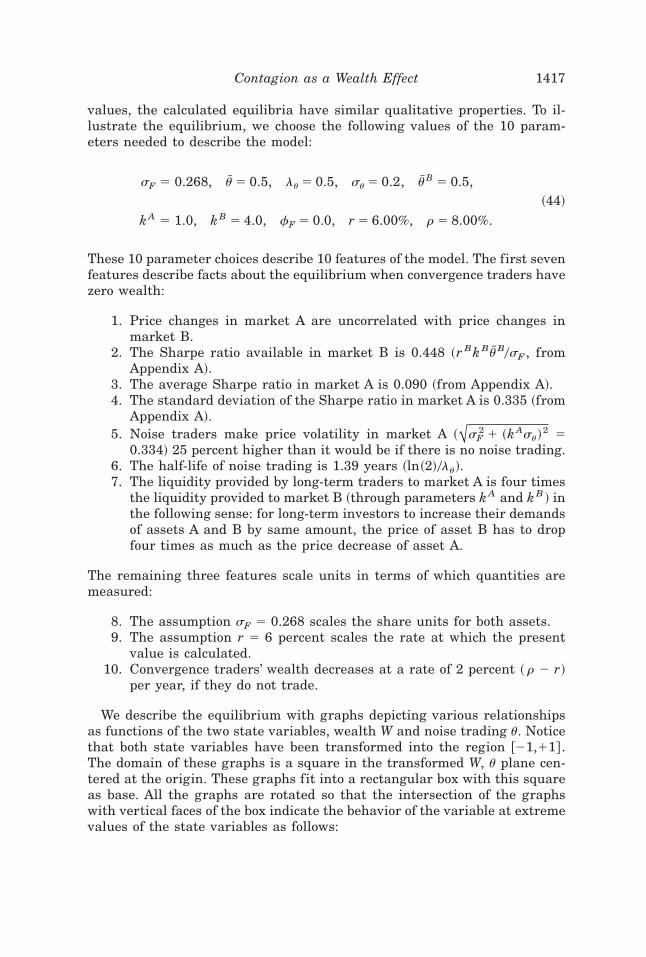
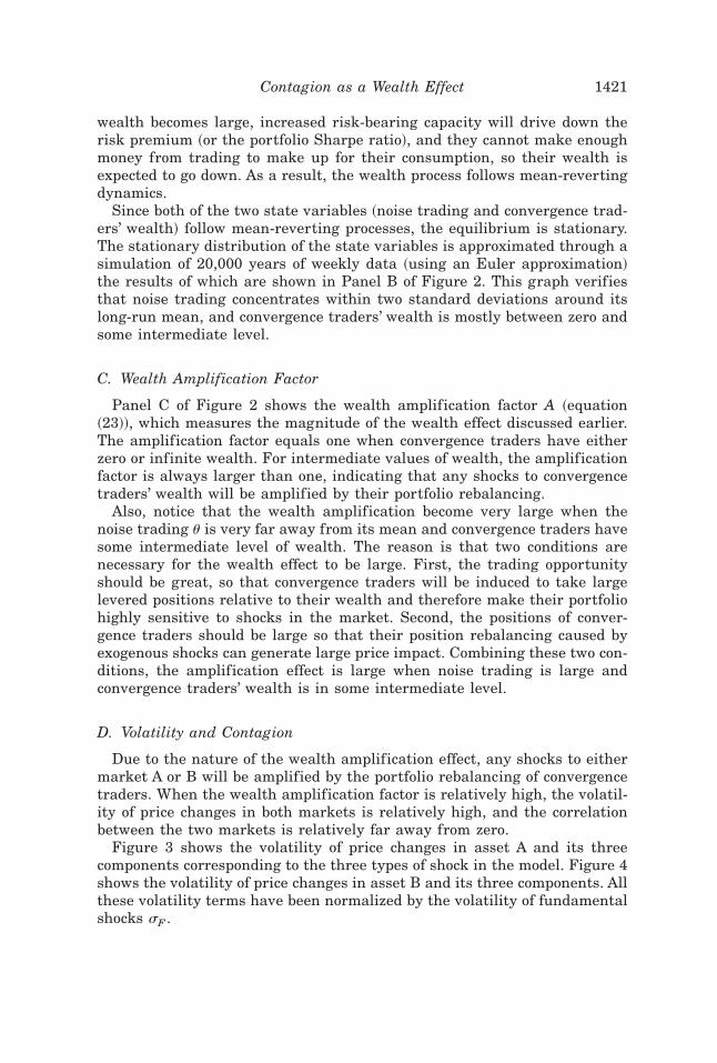
A. Demand Functions and Sharpe Ratios

Panels A and B of Figure 1 show the demand functions of convergencetraders for the two risky assets. The intersection of both graphs and thesoutheast face are horizontal lines at zero, ref lecting the boundary conditionthat convergence traders have a zero aggregate position for both assets whenthey have no wealth. In Panel A, the northwest face contains a 45 degreeline, while in Panel B the northwest face contains a horizontal line at NuB.Both indicate the boundary conditions that convergence traders absorb allthe noise in market A and total supply in market B when they have infinitewealth.

Panels C and D of Figure 1 show the Sharpe ratios of assets A and B. BothSharpe ratios are zero when wealth is infinite. When wealth is zero, PanelC shows that as the position of noise traders varies from long to short, theSharpe ratio on asset A varies ~linearly! over positive and negative values,indicating both long and short positions can be profitable trading opportu-nities by taking the opposite side of noise trading. Panel D shows that whenwealth is zero, the Sharp ratio in market B is a positive constant ~becausesupply is positive! that does not vary with noise trading in market A. Note,however, that for intermediate levels of wealth, the Sharpe ratio in marketB is higher when noise trading in market A is not close to its mean. This isdue to increased correlation between assets A and B when convergence trad-ers have significant positions in both assets. Increased correlation betweenA and B discourages convergence traders from holding asset B when theyhave large positions in asset A. Therefore, a larger risk premium must beoffered in market B to attract convergence traders.

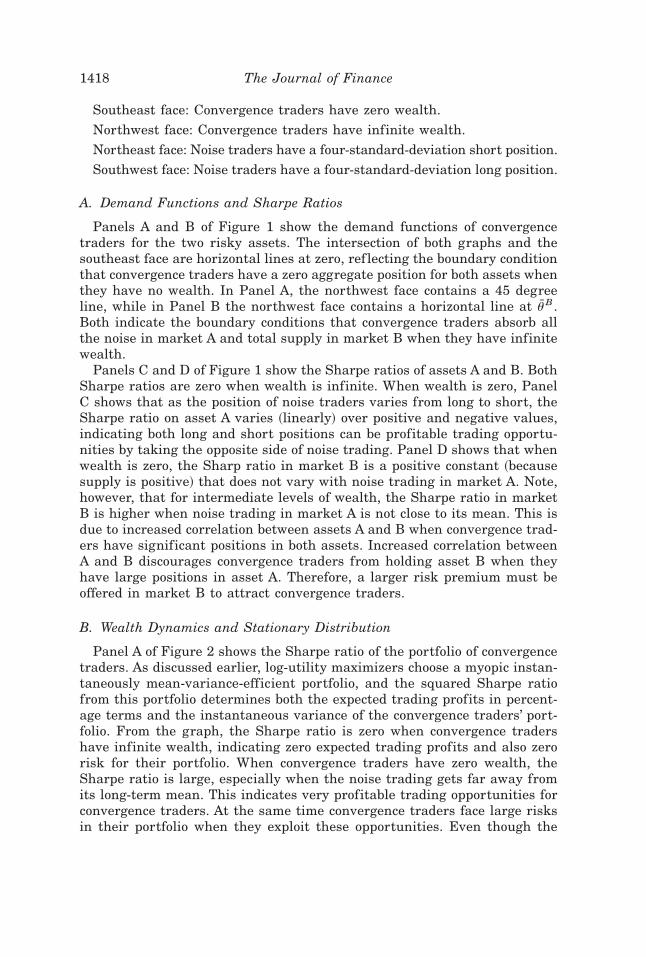
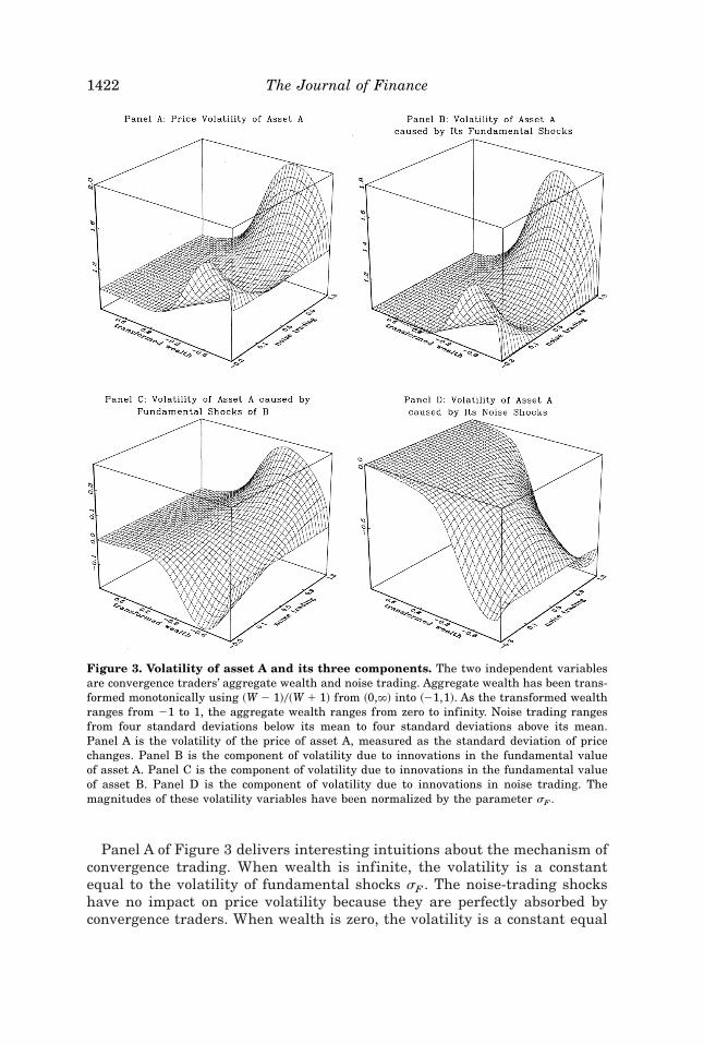
B. Wealth Dynamics and Stationary Distribution

Panel A of Figure 2 shows the Sharpe ratio of the portfolio of convergencetraders. As discussed earlier, log-utility maximizers choose a myopic instan-taneously mean-variance-efficient portfolio, and the squared Sharpe ratiofrom this portfolio determines both the expected trading profits in percent-age terms and the instantaneous variance of the convergence traders’ port-folio. From the graph, the Sharpe ratio is zero when convergence tradershave infinite wealth, indicating zero expected trading profits and also zerorisk for their portfolio. When convergence traders have zero wealth, theSharpe ratio is large, especially when the noise trading gets far away fromits long-term mean. This indicates very profitable trading opportunities forconvergence traders. At the same time convergence traders face large risksin their portfolio when they exploit these opportunities. Even though the


Sharpe ratio of asset A varies from positive to negative, the portfolio Sharperatio is always positive because convergence traders can take a short posi-tion in response to a negative Sharpe ratio.

For a given level of noise trading, the portfolio Sharpe ratio graduallydecreases as convergence traders’ wealth goes up from zero to infinity. Thisis the sense in which convergence trading makes markets efficient. Theincrease of risk bearing capacities among convergence traders reduces the

Figure 1. Demand functions and Sharpe ratios. The two independent variables are con-vergence traders’ aggregate wealth and noise trading. Aggregate wealth has been transformedmonotonically using ~W � 1!0~W � 1! from ~0,`! into ~�1,1!. As the transformed wealth rangesfrom �1 to 1, the aggregate wealth ranges from zero to infinity. Noise trading ranges from fourstandard deviations below its mean to four standard deviations above its mean. Panels A and Bare the equilibrium demands by convergence traders for assets A and B, respectively. Panels Cand D are the equilibrium Sharpe ratios for assets A and B, respectively.


equilibrium risk premium. This property of the Sharpe ratio results in amean-reverting dynamics for the convergence traders’ wealth process. Onthe one hand, when convergence traders’ wealth is low, the trading is soprofitable that their wealth is expected to go up. On the other hand, as their

Figure 2. Sharpe ratio of convergence traders’ portfolio, stationary distribution, wealthamplification factor and correlation. The two independent variables are convergence trad-ers’ aggregate wealth and noise trading. Aggregate wealth has been transformed monotonicallyusing ~W � 1!0~W � 1! from ~0,`! into ~�1,1!. As the transformed wealth ranges from �1 to 1,the aggregate wealth ranges from zero to infinity. Noise trading ranges from four standarddeviations below its mean to four standard deviations above its mean. Panel A is the squaredSharpe ratio of the convergence traders’ aggregate portfolio. Panel B is the stationary distri-bution density of the two state variables, estimated by simulating 20,000 years of equilibriumtrading. Panel C is the amplification factor associated with the convergence traders’ wealtheffect. Panel D is the correlation between price changes of assets A and B.


wealth becomes large, increased risk-bearing capacity will drive down therisk premium ~or the portfolio Sharpe ratio!, and they cannot make enoughmoney from trading to make up for their consumption, so their wealth isexpected to go down. As a result, the wealth process follows mean-revertingdynamics.

Since both of the two state variables ~noise trading and convergence trad-ers’ wealth! follow mean-reverting processes, the equilibrium is stationary.The stationary distribution of the state variables is approximated through asimulation of 20,000 years of weekly data ~using an Euler approximation!the results of which are shown in Panel B of Figure 2. This graph verifiesthat noise trading concentrates within two standard deviations around itslong-run mean, and convergence traders’ wealth is mostly between zero andsome intermediate level.

C. Wealth Amplification Factor

Panel C of Figure 2 shows the wealth amplification factor A ~equation~23!!, which measures the magnitude of the wealth effect discussed earlier.The amplification factor equals one when convergence traders have eitherzero or infinite wealth. For intermediate values of wealth, the amplificationfactor is always larger than one, indicating that any shocks to convergencetraders’ wealth will be amplified by their portfolio rebalancing.

Also, notice that the wealth amplification become very large when thenoise trading u is very far away from its mean and convergence traders havesome intermediate level of wealth. The reason is that two conditions arenecessary for the wealth effect to be large. First, the trading opportunityshould be great, so that convergence traders will be induced to take largelevered positions relative to their wealth and therefore make their portfoliohighly sensitive to shocks in the market. Second, the positions of conver-gence traders should be large so that their position rebalancing caused byexogenous shocks can generate large price impact. Combining these two con-ditions, the amplification effect is large when noise trading is large andconvergence traders’ wealth is in some intermediate level.

D. Volatility and Contagion

Due to the nature of the wealth amplification effect, any shocks to eithermarket A or B will be amplified by the portfolio rebalancing of convergencetraders. When the wealth amplification factor is relatively high, the volatil-ity of price changes in both markets is relatively high, and the correlationbetween the two markets is relatively far away from zero.

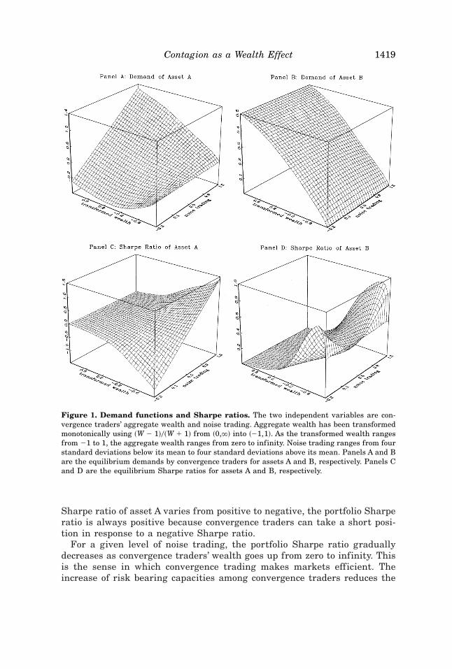
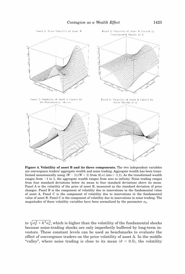
Figure 3 shows the volatility of price changes in asset A and its threecomponents corresponding to the three types of shock in the model. Figure 4shows the volatility of price changes in asset B and its three components. Allthese volatility terms have been normalized by the volatility of fundamentalshocks sF .


Panel A of Figure 3 delivers interesting intuitions about the mechanism ofconvergence trading. When wealth is infinite, the volatility is a constantequal to the volatility of fundamental shocks sF . The noise-trading shockshave no impact on price volatility because they are perfectly absorbed byconvergence traders. When wealth is zero, the volatility is a constant equal

Figure 3. Volatility of asset A and its three components. The two independent variablesare convergence traders’ aggregate wealth and noise trading. Aggregate wealth has been trans-formed monotonically using ~W � 1!0~W � 1! from ~0,`! into ~�1,1!. As the transformed wealthranges from �1 to 1, the aggregate wealth ranges from zero to infinity. Noise trading rangesfrom four standard deviations below its mean to four standard deviations above its mean.Panel A is the volatility of the price of asset A, measured as the standard deviation of pricechanges. Panel B is the component of volatility due to innovations in the fundamental valueof asset A. Panel C is the component of volatility due to innovations in the fundamental valueof asset B. Panel D is the component of volatility due to innovations in noise trading. Themagnitudes of these volatility variables have been normalized by the parameter sF .


to !sF2 � k2su

2, which is higher than the volatility of the fundamental shocksbecause noise-trading shocks are only imperfectly buffered by long-term in-vestors. These constant levels can be used as benchmarks to evaluate theeffect of convergence traders on the price volatility of asset A. In the middle“valley”, where noise trading is close to its mean ~u � 0.5!, the volatility

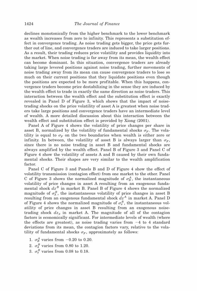
Figure 4. Volatility of asset B and its three components. The two independent variablesare convergence traders’ aggregate wealth and noise trading. Aggregate wealth has been trans-formed monotonically using ~W � 1!0~W � 1! from ~0,`! into ~�1,1!. As the transformed wealthranges from �1 to 1, the aggregate wealth ranges from zero to infinity. Noise trading rangesfrom four standard deviations below its mean to four standard deviations above its mean.Panel A is the volatility of the price of asset B, measured as the standard deviation of pricechanges. Panel B is the component of volatility due to innovations in the fundamental valueof asset A. Panel C is the component of volatility due to innovations in the fundamentalvalue of asset B. Panel C is the component of volatility due to innovations in noise trading. Themagnitudes of these volatility variables have been normalized by the parameter sF .


declines monotonically from the higher benchmark to the lower benchmarkas wealth increases from zero to infinity. This represents a substitution ef-fect in convergence trading. As noise trading gets bigger, the price gets fur-ther out of line, and convergence traders are induced to take larger positions.As a result, their trading reduces price volatility and provides liquidity intothe market. When noise trading is far away from its mean, the wealth effectcan become dominant. In this situation, convergence traders are alreadytaking large levered positions against noise trading, further movements ofnoise trading away from its mean can cause convergence traders to lose somuch on their current positions that they liquidate positions even thoughthe positions are expected to be more profitable. When this happens, con-vergence traders become price destabilizing in the sense they are induced bythe wealth effect to trade in exactly the same direction as noise traders. Thisinteraction between the wealth effect and the substitution effect is exactlyrevealed in Panel D of Figure 3, which shows that the impact of noise-trading shocks on the price volatility of asset A is greatest when noise trad-ers take large positions and convergence traders have an intermediate levelof wealth. A more detailed discussion about this interaction between thewealth effect and substitution effect is provided by Xiong ~2001!.

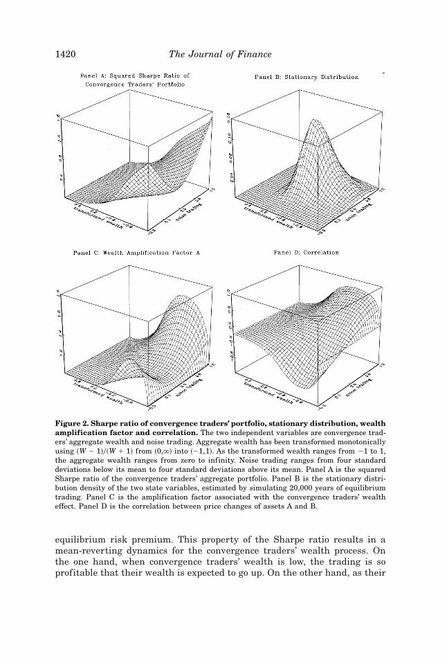
Panel A of Figure 4 shows the volatility of price changes per share inasset B, normalized by the volatility of fundamental shocks sF . The vola-tility is equal to sF on the two boundaries when wealth is either zero orinfinity. In between, the volatility of asset B is always larger than sF ,since there is no noise trading in asset B and fundamental shocks arealways amplified by the wealth effect. Panel B of Figure 3 and Panel C ofFigure 4 show the volatility of assets A and B caused by their own funda-mental shocks. Their shapes are very similar to the wealth amplificationfactor.

Panel C of Figure 3 and Panels B and D of Figure 4 show the effect ofvolatility transmission ~contagion effect! from one market to the other. PanelC of Figure 3 shows the normalized magnitude of sB

A , the instantaneousvolatility of price changes in asset A resulting from an exogenous funda-mental shock dz B in market B. Panel B of Figure 4 shows the normalizedmagnitude of sA

B , the instantaneous volatility of price changes in asset Bresulting from an exogenous fundamental shock dz A in market A. Panel Dof Figure 4 shows the normalized magnitude of su

B , the instantaneous vol-atility of price changes in asset B resulting from an exogenous noise-trading shock dzu in market A. The magnitude of all of the contagionfactors is economically significant. For intermediate levels of wealth ~wherethe effects are greatest!, as noise trading varies from �4 to 4 standarddeviations from its mean, the contagion factors vary, relative to the vola-tility of fundamental shocks sF , approximately as follows:

1. sBA varies from �0.20 to 0.20.

2. sAB varies from 0.80 to 1.20.

3. suB varies from 0.08 to 0.18.


Also notice that the magnitude of sBA is smaller than the magnitude of sA

B.The reason for this is that the Sharpe ratio of asset B is smaller in absolutevalue than that of asset A. Thus, convergence traders take large positionsfor asset A, resulting in larger risk exposure to shocks to asset A. Therefore,shocks in market A can cause larger wealth f luctuations to convergence trad-ers’ portfolio, which are transmitted to the price of asset B in larger mag-nitude than the shocks in market B are transmitted to the price of asset A.

Panel D of Figure 2 shows the correlation between the price changes of thetwo assets. Since the fundamentals and noise trading in the two markets areindependently distributed, nonzero correlation is associated with contagion.When wealth is zero or infinity, correlation is zero. At intermediate values ofwealth, correlation can be significantly different from zero. Correlation is pos-itive when convergence traders are long in both markets, and negative whenconvergence traders are short in market A and long in market B. The magni-tude of the correlation becomes large when noise trading in the market getsfar away from its mean and convergence traders’ wealth is at some intermedi-ate level. These regions are exactly where the wealth amplification effect islarge. As noise trading varies from �4 to 4 standard deviations away from itsmean, correlation at intermediate levels of wealth ranges from �0.6 to � 0.8.

These graphs suggest “crisis” situations when noise trading is far awayfrom its mean and convergence traders’ wealth is at some intermediate level.In these situations, the wealth effect can induce convergence traders to liq-uidate large amounts of positions across their whole portfolio in response tounfavorable shocks, resulting in large price volatility and greatly reducedliquidity in all markets, and large correlation between different markets.These graphs also confirm some of the stylized facts associated with assetprice volatility and correlation between asset prices. First, asset price vola-tility is always larger than fundamental volatility. The additional volatilitycomes from both noise trading and the wealth amplification effect. Second,the correlation between asset prices is larger than the correlation betweenasset fundamentals. This occurs because the wealth dynamics of conver-gence traders introduce an additional common factor among asset prices.Third, asset price volatility and the correlation between asset prices areboth time varying. The stochastic volatility and correlation result from thenonlinear dynamics of the convergence traders’ wealth process.

IV. Implications for Risk Management

Our model has important implications for risk management. The key in-sight is that in equilibrium, the risks are endogenously determined by thetrading of all market participants, and it may be dangerous to treat risks asexogenous in risk management. More specifically, the following cautions canbe drawn from our model. First, risk managers should recognize the wealtheffect of convergence traders who use a short-term trading strategy. Second,risk managers should appreciate the importance of market liquidity pro-vided by long-term investors in periods of crisis. Third, risk managers should


realize that correlation between assets tends to deviate from historical val-ues and rise during crises in such a way that portfolio losses occur in allpositions simultaneously. Failure to recognize these factors in risk manage-ment can result in underestimation of volatility and correlation between as-set prices, especially when the wealth amplification effect is severe.

The importance of these factors has been illustrated by the financial crisisof hedge fund Long Term Capital Management ~LTCM! during 1998. As re-called by one of LTCM’s partners ~Lewis, 1999, p. 31!: “It was as if there wassomeone out there with our exact portfolio, only it was three times as large asours, and they were liquidating all at once.” This suggests a severe copycat prob-lem during this period. Due to the success of LTCM before the crisis, its con-vergence trading strategies were popular among other hedge funds andproprietary trading desks at many investment banks. When LTCM ran intotrouble and needed to liquidate some of their positions, other convergence trad-ers with similar positions were simultaneously trying to dump their positions.When all of these convergence traders were trying to get out of their positionsthrough the only exit, the liquidity provided by long-term investors, the doordid not appear to be as wide as it once was. Furthermore, the liquidation ofconvergence traders’ positions was not limited to only one asset, it was spreadout among all assets in convergence traders’ portfolios due to increased riskaversion. This caused the correlation between asset returns to be much higherthan in usual periods, resulting in the failure of diversification to reduce risksas much as models based on historical returns may suggest. The report by theBIS ~1999! provides a documentation of volatility and correlation across a widerange of financial markets for periods around the crisis of LTCM in 1998.

Our model suggests risk managers take into account the endogenous riskscaused by the trading of other market participants. Since these market-created risks, such as contagion and volatility amplification by the conver-gence traders’ wealth effect, are only evident in extreme scenarios, studyinghistorical data of asset returns and volatility tends to overlook or underesti-mate these risks, unless extremely long series of data are used. Even if verylong series of data are available, the potential changes in the structure ofthe market can make it hopeless to determine these extreme risks fromhistorical data.

To avoid these problems, risk managers should not rely only on statisticalmethods. Our economic model in this paper, based on assumptions about theliquidity provided by long-term investors and the behavior of convergencetraders, suggests that risk managers calculate their optimal risky positionsafter considering the capitalization and positions of other traders in the mar-ket. Therefore, it offers risk managers a different perspective for controllingthese endogenous risks associated with the convergence traders’ wealth ef-fect in extreme situations.

V. Conclusion

In this paper, we develop an equilibrium model of contagion that operatesthrough a wealth effect of convergence traders. Convergence traders special-


ize in trading a small number of assets in which they take large risky po-sitions against noise trading. Wealth effect occurs when convergence traderssuffer large capital losses due to unfavorable shocks and need to liquidatepositions across their portfolio. Their position liquidation can cause the orig-inal shocks to be greatly amplified and transmitted from one asset to otherassets.

In equilibrium, the asset price dynamics and convergence traders’ wealthdynamics are simultaneously determined. This simultaneous relationship in-troduces endogenous risks into the model in the form of contagion and vol-atility amplification through the wealth effect of convergence traders. Ourmodel cautions risk managers to take into account these endogenous risks.Failure to do so can cause much larger risks in trading than what is forecastby naive statistical tools. Our economic model, based on assumptions aboutthe liquidity provided by long-term investors and the behavior of conver-gence traders, suggests a direction of future research which could lead tobetter tools for risk management.

Appendix A. Derivation of Asset Return Processes

Given the aggregate portfolio policies X A~u,W ! and X B~u,W ! for conver-gence traders, we derive asset return processes by applying Ito’s lemma. Themarket clearing condition gives the price functions for the two assets:

P A � F A � kA~u� X A !, ~A1!

P B � F B � kB~ NuB � X B !. ~A2!

The excess return process for investing in one share of asset A is given by

dQA � dP A � ~DA � rP A !dt

� sF dz A � kAdu� kAdX A � rkA~u� X A !dt.~A3!

Similarly, the excess return for investing in one share of asset B is

dQB � sF dz B � kBdX B � rkB~ NuB � X B !dt. ~A4!

As discussed in Section II, we assume without loss of generality that thefundamental process of the two assets have the same fundamental volatilitysF . From Ito’s lemma, we obtain

dX A � XuA du� 102Xuu

A E~du!2 � XWA dW � 102XWW

A E~dW !2 � XuWA E~dudW !,

~A5!

dX B � XuB du� 102Xuu

B E~du!2 � XWB dW � 102XWW

B E~dW !2 � XuWB E~dudW !.

~A6!


The asset return processes and convergence traders’ wealth process are si-multaneously determined in the equilibrium. Equations ~A1! through ~A4!show the dependence of return processes dQA and dQB on convergence trad-ers’ aggregate wealth W. On the other hand, convergence traders’ wealthdepends on the return processes through their budget constraint

dW � X AdQA � X BdQB � ~rW � C!dt. ~A7!

To deal with this circular relationship, we first substitute equation ~A7! intoequations ~A5! and ~A6!, then further substitute equations ~A5! and ~A6!into equations ~A3! and ~A4!. Finally, we obtain a set of two linear equationsfor dQA and dQB :

~1 � kAX AXWA !dQA � kAXW

A X BdQB

� sF dzA � kA~1 � XuA!du� @rkA~u� X A !� kAXW

A ~rW � C!#dt

�kA

2Xuu

A E~du!2 �kA

2XWW

A E~dW !2 � kAXuWA E~dudW ! ~A8!

� kBX AXWB dQA � ~1 � kBX BXW

B !dQB

� sF dzB � kBXuB du� @kBXW

B ~rW � C!� rkB~ NuB � X B !#dt

�kB

2Xuu

B E~du!2 �kB

2XWW

B E~dW !2 � kBXuWB E~dudW !.

~A9!

Solution to these linear equations gives us the following return processes:

dQA � mAdt � sAA dz A � sB

A dz B � suA dzu , ~A10!

sAA � sF ~1 � kBX BXW

B !A~u,W !, ~A11!

sBA � sF kAX BXW

A A~u,W !, ~A12!

suA � �kAsu @~1 � Xu


A X BXuB#A~u,W !, ~A13!

mA � A~u,W !$kAlu~u� Nu!@~1 � XuA!~1 � kBX BXW

B !� kBXWA X BXu

B#

� kAXWA ~rW � C!� rkA~1 � kBX BXW

B !~u� X A !

� rkAkBXWA X B~ NuB � X B !%

�kAsu

2

2@Xuu

A ~1 � kBX BXWB !� kBXW

A X BXuuB #A~u,W ! ~A14!

�kA~sW !2

2@XWW


A X BXWWB #A~u,W !

� kAsusuW@XuW


A X BXuWB #A~u,W !,


dQB � mBdt � sAB dz A � sB

B dz B � suB dzu , ~A15!

sAB � sF kBX AXW

B A~u,W !, ~A16!

sBB � sF @1 � kAX AXW

A #A~u,W !, ~A17!

suB � kBsu @Xu


B ~1 � XuA!#A~u,W !, ~A18!

mB � A~u,W !$�kBlu~u� Nu!@XuB~1 � kAX AXW

A !� kAX AXWB ~1 � Xu

A!#

� kBXWB ~rW � C!� rkB~1 � kAX AXW

A !~ NuB � X B !

� rkAkBX AXWB ~u� X A !%

�kBsu

2

2@Xuu

B ~1 � kAX AXWA !� kAX AXuu

A XWB #A~u,W ! ~A19!

�kB~sW !2

2@XWW

B ~1 � kAX AXWA !� kAX AXWW

A XWB #A~u,W !

� kBsusuW@XuW

B ~1 � kAX AXWA !� kAX AXuW

A XWB #A~u,W !.

In the expressions above, the common term

A~u,W ! �1

1 � kAX AXWA � kBX BXW

B ~A20!

represents the wealth amplification factor. The total volatility of these re-turns is

sA � !~sAA!2 � ~sB

A!2 � 2fFsAAsB

A � ~suA!2, ~A21!

sB � !~sAB!2 � ~sB

B!2 � 2fFsABsB

B � ~suB!2. ~A22!

The instantaneous correlation between the two return processes is

f �1

sAsB @sAAsA

B � sBAsA

B � fF ~sAAsB

B � sBAsA

B!� suAsu

B# . ~A23!

From the budget constraints, we can derive the process for convergencetraders’ aggregate wealth:

dW � mWdt � sAW dz A � sB

W dz B � suW dzu , ~A24!

mW � X AmA � X BmB � rW � C, ~A25!

sAW � X AsA

A � X BsAB , ~A26!

sBW � X AsB

A � X BsBB , ~A27!

suW � X Asu

A � X BsuB . ~A28!


The total volatility of the wealth process is

sW � !~sAW!2 � ~sB

W!2 � 2fFsAWsB

W � ~suW!2. ~A29!

It is useful to show the return processes when the effect of convergencetraders is small ~X A r 0, X B r 0!. Under this situation, the excess returnprocesses are

dQA � sF dz A � kAdu� rkAudt, ~A30!

dQB � sF dz B � rkB NuBdt. ~A31!

Sharpe ratios of asset A and B are

mA

sA �rkAu� kAlu~u� Nu!

!sF2 � ~kAsu!

2, ~A32!

mB

sB �rkB NuB

sF. ~A33!

The Sharpe ratio of asset A f luctuates with its supply u, and the variance ofthe Sharpe ratio is

Var�mA

sA� �~r � lu!

2~kA !2su2

2lu @sF2 � ~kAsu!

2 #. ~A34!

These return processes represent the original trading opportunities whenthere are no convergence traders at all.

Appendix B. Derivation of Optimal Strategy

In this section, we derive convergence traders’ optimal trading strategygiven the return processes of assets A and B. We can write the asset returnprocesses in the following form:

dQA � mA~u,W !dt � sAA~u,W !dz A � sB

A~u,W !dz B � suA~u,W !dzu , ~B1!

dQB � mB~u,W !dt � sAB~u,W !dz A � sB

B~u,W !dz B � suB~u,W !dzu . ~B2!

These return processes represent the trading opportunities to an individualconvergence trader, and these processes depend on the two state variables uand W. The parameter u denotes the supply shock to asset A. It follows

du � �lu~u� Nu!dt � sudzu .


The parameter W is the aggregate wealth of convergence traders, and itfollows the process

dW � mW~u,W !dt � sAW~u,W !dz A � sB

W~u,W !dz B � suW dzu . ~B3!

We denote an individual convergence trader ’s portfolio choices, consump-tion, and wealth as X i A

, X i B, C i, and W i, respectively. The convergence

trader ’s budget constraint is

d RW � X i AdQA � X i B

dQB � ~rW i � C i !dt. ~B4!

The convergence trader maximizes her lifetime utility given by

J~W i,u,W ! � max$X iA, X iB,C i %

Et�0

`

e�rs ln~Ct�si ! ds. ~B5!

We solve the portfolio and consumption policies through a Bellman equationas developed by Merton ~1971!. The Bellman equation can be derived as

rJ~W i,u,w! � max$X iA, X iB,C i %

@ ln~C i !� L0J #

� maxX iA, X iB,C i

@ ln~C i !� JW i ~X i AmA � X i B

mB � rW i � C i !

� 102JW iW i ~~X i A!2~sA !2 � ~X i B

!2~sB !2

� 2X i AX i BfsAsB ! ~B6!

� lu~ Nu� u!Ju� mWJW � 102su2 Juu� 102sW

2 JWW

� JW iuE~dW idu!0dt � JW iwE~dW idW !0dt

� JuwE~dudW !0dt# ,

where L0 is the drift operator, and f is the instantaneous correlation be-tween dQA and dQB. The value function of a logarithmic utility maximizercan be specified as

J~W i,u,w! �1

rln~W i !� j~u,W !. ~B7!

The first order condition of the Bellman equation gives the optimal portfolioand consumption policies:

X i A�

W i

1 � f2 � mA

~sA !2� f

mB

sAsB �, ~B8!

X i B�

W i

1 � f2 � mB

~sB !2� f

mA

sAsB �, ~B9!

C i � rW i. ~B10!


After substituting the optimal policies into the Bellman equation, W i dis-appears from both sides of the equation, and the Bellman equation collapsesinto a partial differential equation in u and W only:

rj~u,W ! � ln~ r!� r~r � r!�r

2~1 � f2 !� ~mA !2

~sA !2� 2f

mAmB

sAsB �~mB !2

~sB !2�

� lu~ Nu� u! ju� mWjW � 102su2 juu� 102sW

2 jWW � susuW juW .

~B11!

Therefore, the convergence trader ’s policy functions and value function be-come separated. The solution to the PDE of the value function exists undercertain technical conditions. We will focus on the policy functions and dis-cuss the equilibrium of asset markets.

It is a well-known result of logarithmic utility that log-utility maximizersdo not have any hedging need. Their portfolio and consumption policies aresolely determined by their current trading opportunities and their wealth.For a general utility maximizer, the hedging need is represented by thedependence of policy functions on the value function. The assumption of log-arithmic utility for convergence traders greatly simplifies the problem with-out losing the key feature of our model, which is the wealth effect.

Notice that log-utility maximizers hold a locally mean-variance efficientportfolio. It is easy to derive the instantaneous expected trading profits andvariance of this portfolio:

E� X i A

W i dQA �X i B

W i dQB� � var� X i A

W i dQA �X i B

W i dQB��

1

1 � f2 � ~mA !2

~sA !2�~mB !2

~sB !2� 2f

mAmB

sAsB �.

~B12!

This value is exactly the squared Sharpe ratio of the instantaneous mean-variance efficient portfolio.

Appendix C. Partial Differential Equations

Appendix C presents the partial differential equations from the fixed-point problem. Given convergence traders’ aggregate portfolio and consump-tion functions X~u,W ! and C~u,W !, the optimal aggregate portfolio andconsumption rules can be easily derived from equations ~B8! through ~B10!by replacing W i by W:

X *A

�W

1 � f2 � mA

~sA !2� f

mB

sAsB �, ~C1!

X *B

�W

1 � f2 � mB

~sB !2� f

mA

sAsB �, ~C2!

C � rW. ~C3!


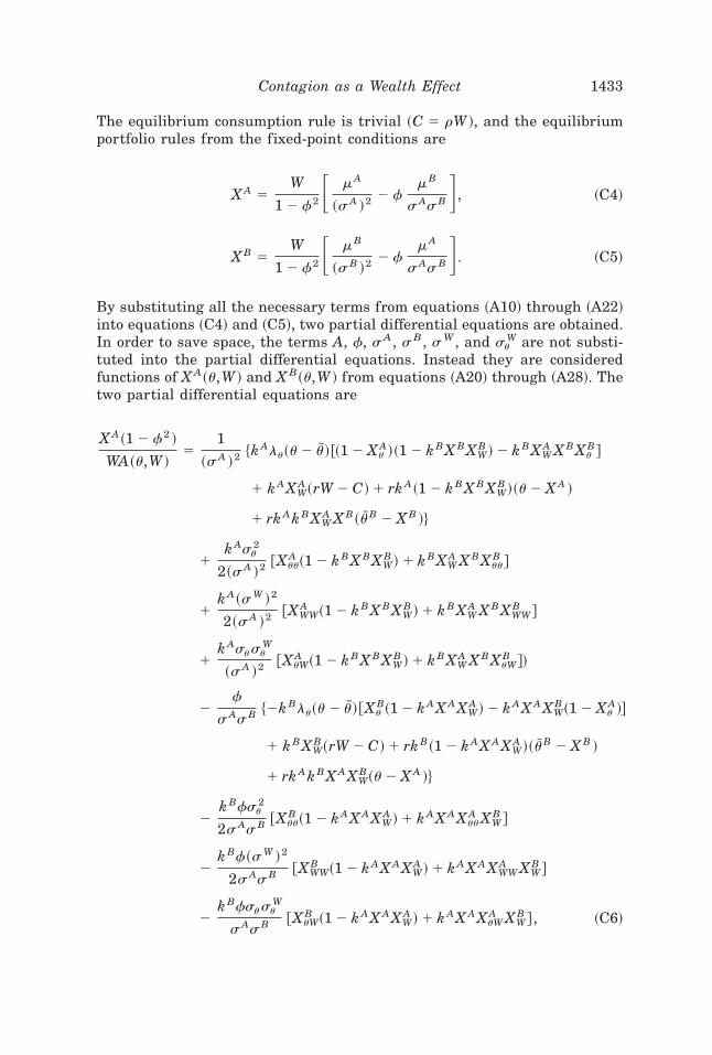
The equilibrium consumption rule is trivial ~C � rW !, and the equilibriumportfolio rules from the fixed-point conditions are

X A �W

1 � f2 � mA

~sA !2� f

mB

sAsB �, ~C4!

X B �W

1 � f2 � mB

~sB !2� f

mA

sAsB �. ~C5!

By substituting all the necessary terms from equations ~A10! through ~A22!into equations ~C4! and ~C5!, two partial differential equations are obtained.In order to save space, the terms A, f, sA, sB, sW, and su

W are not substi-tuted into the partial differential equations. Instead they are consideredfunctions of X A~u,W ! and X B~u,W ! from equations ~A20! through ~A28!. Thetwo partial differential equations are

X A~1 � f2 !

WA~u,W !�

1

~sA !2$kAlu~u� Nu!@~1 � Xu


A X BXuB#


B !~u� X A !


�kAsu

2

2~sA !2@Xuu


A X BXuuB #

�kA~sW !2

2~sA !2@XWW


A X BXWWB #

�kAsusu

W

~sA !2@XuW


A X BXuWB #!

�f

sAsB $�kBlu~u� Nu!@XuB~1 � kAX AXW

A !� kAX AXWB ~1 � Xu

A!#


A !~ NuB � X B !


�kBfsu

2

2sAsB @XuuB ~1 � kAX AXW

A !� kAX AXuuA XW

B #

�kBf~sW !2

2sAsB @XWWB ~1 � kAX AXW

A !� kAX AXWWA XW

B #

�kBfsusu

W

sAsB @XuWB ~1 � kAX AXW

A !� kAX AXuWA XW

B # , ~C6!


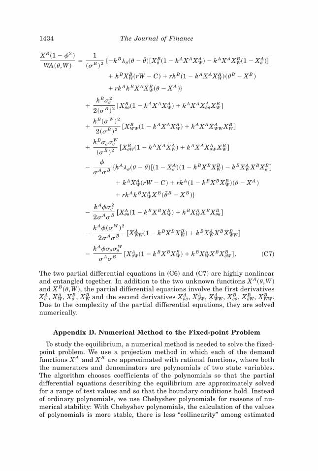
X B~1 � f2 !

WA~u,W !�

1

~sB !2$�kBlu~u� Nu!@Xu


B ~1 � XuA!#


A !~ NuB � X B !


�kBsu

2

2~sB !2@Xuu

B ~1 � kAX AXWA !� kAX AXuu

A XWB #

�kB~sW !2

2~sB !2@XWW

B ~1 � kAX AXWA !� kAX AXWW

A XWB #

�kBsusu

W

~sB !2@XuW

B ~1 � kAX AXWA !� kAX AXuW

A XWB #

�f

sAsB $kAlu~u� Nu!@~1 � Xu


A X BXuB#


B !~u� X A !


�kAfsu

2

2sAsB @XuuA ~1 � kBX BXW

B !� kBXWA X BXuu

B #

�kAf~sW !2

2sAsB @XWWA ~1 � kBX BXW

B !� kBXWA X BXWW

B #

�kAfsusu

W

sAsB @XuWA ~1 � kBX BXW

B !� kBXWA X BXuW

B # . ~C7!

The two partial differential equations in ~C6! and ~C7! are highly nonlinearand entangled together. In addition to the two unknown functions X A~u,W !and X B~u,W !, the partial differential equations involve the first derivativesXu

A , XWA , Xu

B , XWB and the second derivatives Xuu

A , XuWA , XWW

A , XuuB , XuW

B , XWWB .

Due to the complexity of the partial differential equations, they are solvednumerically.

Appendix D. Numerical Method to the Fixed-point Problem

To study the equilibrium, a numerical method is needed to solve the fixed-point problem. We use a projection method in which each of the demandfunctions X A and X B are approximated with rational functions, where boththe numerators and denominators are polynomials of two state variables.The algorithm chooses coefficients of the polynomials so that the partialdifferential equations describing the equilibrium are approximately solvedfor a range of test values and so that the boundary conditions hold. Insteadof ordinary polynomials, we use Chebyshev polynomials for reasons of nu-merical stability: With Chebyshev polynomials, the calculation of the valuesof polynomials is more stable, there is less “collinearity” among estimated


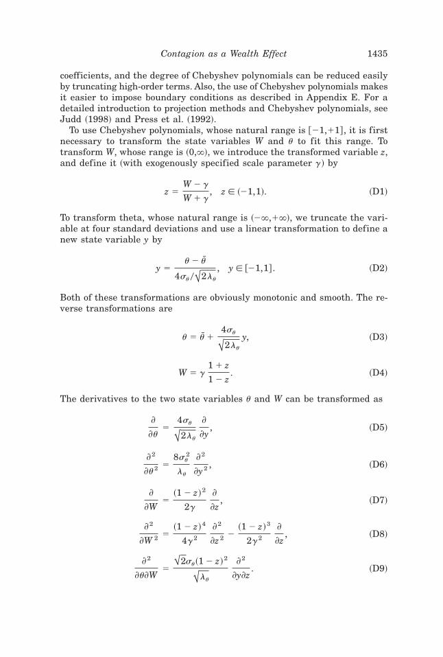
coefficients, and the degree of Chebyshev polynomials can be reduced easilyby truncating high-order terms. Also, the use of Chebyshev polynomials makesit easier to impose boundary conditions as described in Appendix E. For adetailed introduction to projection methods and Chebyshev polynomials, seeJudd ~1998! and Press et al. ~1992!.

To use Chebyshev polynomials, whose natural range is @�1,�1# , it is firstnecessary to transform the state variables W and u to fit this range. Totransform W, whose range is ~0,`!, we introduce the transformed variable z,and define it ~with exogenously specified scale parameter g! by

z �W � g

W � g, z � ~�1,1!. ~D1!

To transform theta, whose natural range is ~�`,�`!, we truncate the vari-able at four standard deviations and use a linear transformation to define anew state variable y by

y �u� Nu

4su 0!2lu, y � @�1,1# . ~D2!

Both of these transformations are obviously monotonic and smooth. The re-verse transformations are

u � Nu�4su

!2luy, ~D3!

W � g1 � z

1 � z. ~D4!

The derivatives to the two state variables u and W can be transformed as

?

?u�

4su

!2lu

?

?y, ~D5!

?2

?u2 �8su

2

lu

?2

?y2 , ~D6!

?

?W�~1 � z!2

2g

?

?z, ~D7!

?2

?W 2 �~1 � z!4

4g2

?2

?z 2 �~1 � z!3

2g2

?

?z, ~D8!

?2

?u?W�!2su~1 � z!2

!lu?2

?y?z. ~D9!


With these formulas, we can transform the original PDEs of X A~u,W ! andX B~u,W ! in equations ~C6! and ~C7! into PDEs of X A~ y, z! and X B~ y, z!.

We approximate the equilibrium demand functions X A~ y, z! and X B~ y, z!as

X A~ y, z! �

(i�j�nu

A

auA~i, j !Ti ~ y!Tj ~z!

(i�j�nd

A

adA~i, j !Ti ~ y!Tj ~z!

, ~D10!

X B~ y, z! �

(i�j�nu

B

auB~i, j !Ti ~ y!Tj ~z!

(i�j�nd

B

adB~i, j !Ti ~ y!Tj ~z!

, ~D11!

where Ti~! is ith order Chebyshev polynomial, and nuA , nd

A , nuB , and nd

B are thetotal orders of polynomials in the numerators and denominators of X A andX B. Let $au

A~i, j !%i�j�nuA , $ad ~i, j !A %i�j�nd

A , $auB~i, j !%i�j�nu

B , and $ad ~i, j !B %i�j�ndB

denote the expansion coefficients. The total number of coefficient is

~nuA � 1!~nu

A � 2!

2�~nd

A � 1!~ndA � 2!

2�~nu

B � 1!~nuB � 2!

2�~nd

B � 1!~ndB � 2!

2.

In terms of these state variables, the boundary conditions now hold forz � �1 ~zero wealth! and z � �1 ~infinite wealth!. Furthermore, the boundaryconditions are actually linear in terms of the transformed state variables, sofor the purpose of estimating the coefficient parameters, they can be imple-mented as linear constraints on the coefficients in the Chebyshev polynomi-als.Appendix E explains in detail how the boundary conditions are implemented.

To capture the nonlinearities in the demand functions and the interactionsbetween the two state variables, we found it necessary to use high-orderpolynomials. Let nu

A , nuB , nd

A , ndB denote the total orders ~maximum sum of

powers of the two state variables! of the polynomials in the numerators ~sub-script u! and denominators ~subscript d! of the estimated equilibrium de-mand functions X A and X B, respectively. Then the total number of coefficientparameters needed to specify both demand functions is

~nuA � 1!~nu

A � 2!

2�~nd

A � 1!~ndA � 2!

2�~nu

B � 1!~nuB � 2!

2�~nd

B � 1!~ndB � 2!

2.

The boundary conditions, implemented as linear constraints on the coeffi-cients, reduce the number of coefficient parameters by 2nu

A � 2ndA � 2nu

B �2nd

B � 4. In our numerical implementation, we let the degree of both numer-ator and denominator in X A be 12 and the degree of both numerator and


denominator of X B be 10. This results in 314 coefficients. The constraintsimplied by the boundary conditions reduce this number by 92. Thus, weestimate 222 coefficient parameters.

To estimate the coefficients, we minimize the sum of squared errors in thepartial differential equations over a fixed set of test points. We noticed thatthe demand functions appear to have more curvature near the boundariesz � �1 and z � �1, so instead of using a uniformly spaced grid of test pointsin the transformed state variables, we increased the number of points nearthe boundaries. We chose a grid size of 21 ~for variable y! by 100 ~for vari-able z!, so the partial differential equations are evaluated at 2,100 points.Since there are 222 parameters to estimate, the system is overdetermined bya factor of roughly 10.

On each test point, two types of error functions have been used at thesame time. One is defined as

Error1 � �� X A � X *A

su�2

� � X B � X *B

su�2

, ~D12!

the difference between the given strategy $X A, X B % and the optimal strategy$X *A, X *B % normalized by the volatility of noise trading and the total supplyof asset B. Since the magnitude of demand is very small when convergencetraders’ capital is small, this way of calculating error underestimates thepercentage errors to arbitrageurs’ portfolio over the region where the arbi-trageurs’ wealth is small. The other error function is defined as

Error2 �sF!~X A � X *A !2 � ~X B � X *B !2

W, ~D13!

the difference between the percentage wealth volatility caused by the fun-damental shocks using $X A, X B % and $X *A, X *B % . Since this error function isdefined by the percentage of wealth, it can correctly estimate errors over theregion where arbitrageurs’ wealth is small, but it may underestimate theabsolute errors to market clearing condition over the region where arbi-trageurs’ wealth is large ~where the demands are small relative to arbi-trageurs’ wealth W !. To give precise estimates of the numerical errors overall regions, a combination of these two types of errors is used:

Error � !Error12 � Error22. ~D14!

To solve the minimization problem, a Levenberg–Marquart algorithm isused. Despite the use of Chebyshev polynomials, the Hessian in our problemis not well behaved because of the linear constraints. Therefore, a gradientmethod has the potential to work better than Newton’s method. TheLevenberg–Marquart algorithm is designed to adjust smoothly between thesetwo methods and thus deals with this problem.


We also notice that as the degree of the polynomial expansion goes up,estimation works better if X A is estimated holding X B fixed and vice versa.We therefore estimate each demand function separately ~holding the otherfixed!. From our experience, the algorithm converges to stable estimatesfor both demand functions after a few iterations. There seems to be acollinearity problem between X A and X B that this approach deals witheffectively.

For the example described below, the numerical error of the fixed-pointproblem is about 10�3, which is interpreted as the maximum difference be-tween the given strategies of convergence traders X A, X B and optimal strat-egies X *A, X *B. We take this as an indication that our numerical algorithmhas found an equilibrium.

Appendix E. Boundary Constraints

The boundary conditions are linear to the after-transformation state vari-ables y:

X A~ y,1! � Nu�4su

!2luT1~ y!, ~E1!

X B~ y,1! � Nu, ~E2!

X A~ y,�1! � 0, ~E3!

X B~ y,�1! � 0. ~E4!

Due to the properties of Chebyshev polynomials, we have Tj~1! � 1 andTj~�1! � ~�1! j. The functions of X A and X B in equations ~D10! and ~D11!become an expansion of y only when z � 1 or z � �1. To match the coef-ficient of y on the two bounds with the boundary conditions ~E1! through~E4!, we obtain a series of constraints on expansion coefficients. Theselinear constraints can be implemented by determining the first two col-umns of the expansion coefficients from the rest of the columns of thoseexpansion coefficients. For the sake of space, these constraints are notlisted here. In this way, the total number of parameters is reduced by2nu

A � 2ndA � 2nu

B � 2ndB � 4 ~first two columns of these four coefficient

matrices!. Therefore, the total number of parameters needed to specifyboth demand functions X A and X B is

nuA~nu

A � 1!

2�

ndA~nd

A � 1!

2�

nuB~nu

B � 1!

2�

ndB~nd

B � 1!

2. ~E5!


REFERENCES

Allen, Franklin, and Douglas Gale, 2000, Financial contagion, Journal of Political Economy108, 1–33.

Ang, Andrew, and Joseph Chen, 2000, Asymmetric correlations of equity portfolios, Mimeo,Columbia University.

Bae, Kee-Hong, Andrew Karolyi, and René Stulz, 2000, A new approach to measuring financialcontagion, Mimeo, Ohio State University.

Balyeat, Brian, and Jayaram Muthuswamy, 1999, The portfolio properties of extreme returns,Mimeo, Texas A&M University.

Bank for International Settlements, 1999, A Review of Financial Market Events in Autumn1998 ~Bank for International Settlements, Basle, Switzerland!.

Basak, Suleyman, 1995, A general equilibrium model of portfolio insurance, Review of Finan-cial Studies 8, 1059–1090.

Breeden, Douglas, 1979, An intertemporal asset pricing model with stochastic consumption andinvestment opportunities, Journal of Financial Economics 7, 265–296.

Caballero, Ricardo, and Arvind Krishnamurthy, 2000, Emerging market crises: An asset mar-kets perspective, Mimeo, Northwestern University.

Calvo, Guillermo, 1999, Contagion in emerging markets: When Wall Street is a carrier, Mimeo,University of Maryland.

Calvo, Guillermo, and Enrique Mendoza, 2000, Rational contagion and the globalization ofsecurities markets, Journal of International Economics 51, 79–113.

Campbell, John, and Albert Kyle, 1993, Smart money, noise trading and stock price behaviour,Review of Economic Studies 60, 1–34.

Connolly, Robert, and Albert Wang, 1998, International equity market comovements: Economicfundamentals or contagion? Mimeo, Rice University.

Connolly, Robert, and Albert Wang, 2000, On stock market return co-movements: Macroeco-nomic news, dispersion of beliefs, and contagion, Mimeo, Rice University.

Danielsson, Jon, 2000, The emperor has no clothes: Limits to risk modeling, Mimeo, LSE.Dornbusch, Rodiger, Yung Chul Park, and Stijn Claessens, 2000, Contagion: How it spreads and

how it can be stopped, Mimeo, MIT.Epstein, Larry, and Tan Wang, 1994, Intertemporal asset pricing under Knightian uncertainty,

Econometrica 62, 283–322.Fleming, Jeff, Chris Kirby, and Barbara Ostdiek, 1998, Information and volatility linkages in

the stock, bond, and money markets, Journal of Financial Economics 49, 111–137.Forbes, Kristin, and Roberto Rigobon, 1999, No contagion, only interdependence: Measuring

stock market co-movements, Mimeo, MIT.Goldstein, Itay, and Ady Pauzner, 2000, Contagion of self-fulfilling financial crises, Mimeo, Tel

Aviv University.Graham, Benjamin, 1973, The Intelligent Investor ~Harper & Row, Publishers, New York!.Gromb, Denis, and Dimitri Vayanos, 2000, Equilibrium and welfare in markets with financially

constrained arbitrageurs, Mimeo, MIT.Grossman, Sanford, and Z. Zhou, 1996, Equilibrium analysis of portfolio insurance, Journal of

Finance 51, 1379–1403.Hamao, Yasushi, Ronald Masulis, and Victor Ng, 1990, Correlation in price changes and vola-

tility across international stock markets, Review of Financial Studies 3, 281–307.Hansen, Lars, Tom Sargent, and T. Tallarini, 1999, Robust permanent income and pricing,

Review of Economic Studies 66, 873–907.Judd, Kenneth, 1998, Numerical Methods in Economics ~MIT Press, Cambridge, MA!.Kaminsky, Graciela, and Carmen Reinhart, 2000, The center and the periphery: Tales of finan-

cial turmoil, Mimeo, University of Maryland.Karolyi, Andrew, and René Stulz, 1996, Why do markets move together? An investigation of

U.S.-Japan stock return co-movements, Journal of Finance 51, 951–986.King, Mervyn, Enrique Sentana, and Sushil Wadhwani, 1994, Volatility and links between

national stock markets, Econometrica 62, 901–933.


King, Mervyn, and Sushil Wadhwani, 1990, Transmission of volatility between stock markets,Review of Financial Studies 3, 5–33.

Kodres, Laura, and Matthew Pritsker, 1998, A rational expectations model of financial conta-gion, Working paper, IMF.

Lagunoff, Roger, and Stacey Schreft, 1998, A model of financial fragility, Mimeo, GeorgetownUniversity.

Lewis, Michael, 1999, How the eggheads cracked, The New York Times Magazine, January 24,24–35.

Lin, Wen-Ling, Robert Engle, and Takatoshi Ito, 1994, Do bulls and bears move across borders?International transmission of stock returns and volatility, Review of Financial Studies 7,507–538.

Longin, Francois, and Bruno Solnik, 1995, Is the correlation in international equity returnsconstant: 1960 to 1990, Journal of International Money and Finance 14, 3–26.

Longin, Francois, and Bruno Solnik, 2001, Extreme correlation of international equity markets,Journal of Finance 56, 649–676.

Masson, Paul, 1998, Contagion: Monsoonal effects, spillovers, and jumps between multiple equi-libria, Working paper, IMF.

Merton, Robert, 1971, Optimum consumption and portfolio rules in a continuous-time model,Journal of Economic Theory 3, 373–413.

Merton, Robert, 1987, A simple model of capital market equilibrium with incomplete informa-tion, Journal of Finance 42, 483–510.

Morris, Stephen, and Hyun Song Shin, 2000, Market risk with interdependent choice, Mimeo,Nuffield College, Oxford University.

Pindyck, Robert, and Julio Rotemberg, 1990, The excess co-movement of commodity prices,Economic Journal 100, 1173–1189.

Pindyck, Robert, and Julio Rotemberg, 1993, The comovement of stock prices, Quarterly Jour-nal of Economics 108, 1073–1104.

Press, William, Saul Teukolsky, William Vetterling, and Brian Flannery, 1992, Numerical Rec-ipes in Fortran ~Cambridge University Press, Cambridge, U.K.!.

Rochet, Jean-Charles, and Jean Tirole, 1996, Interbank lending and systematic risk, Journal ofMoney, Credit and Banking 28, 733–762.

Schinasi, Garry, and Todd Smith, 1999, Portfolio diversification, leverage, and financial conta-gion, Working paper, IMF.

Shiller, Robert, 1989, Comovement in stock prices and comovements in dividends, Journal ofFinance 44, 719–729.

Shleifer, Andrei, and Robert Vishny, 1997, The limits of arbitrage, Journal of Finance 52, 35–55.Wang, Jiang, 1993, A model of intertemporal asset prices under asymmetric information, Re-

view of Economic Studies 60, 249–282.Xiong, Wei, 2001, Convergence trading with wealth effects: An amplification mechanism in

financial markets, Journal of Financial Economics, forthcoming.Yuan, Kathy, 1999, Asymmetric price movements and borrowing constraints, Mimeo, MIT.


Documents

Contagion as a Wealth Effect - Princeton Universitywxiong/papers/contagion.pdf · financial intermediaries to withdraw from illiquid investments. Caballero and Krishnamurthy ~2000!