Embed Size (px)
Citation preview

INDIVIDUAL STUDY
Contact Modelling
Submitted by:
PRUTHVI R VENKAYALA
UFID: 9831-1764
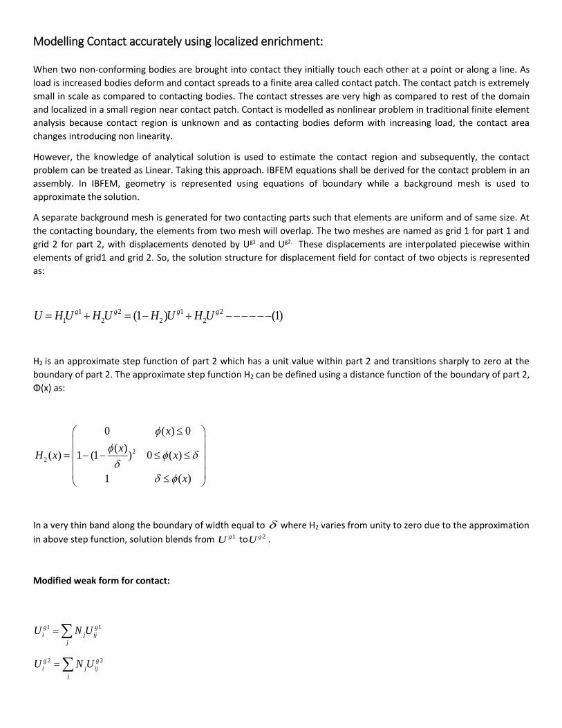
Modelling Contact accurately using localized enrichment:
When two non-conforming bodies are brought into contact they initially touch each other at a point or along a line. As
load is increased bodies deform and contact spreads to a finite area called contact patch. The contact patch is extremely
small in scale as compared to contacting bodies. The contact stresses are very high as compared to rest of the domain
and localized in a small region near contact patch. Contact is modelled as nonlinear problem in traditional finite element
analysis because contact region is unknown and as contacting bodies deform with increasing load, the contact area
changes introducing non linearity.
However, the knowledge of analytical solution is used to estimate the contact region and subsequently, the contact
problem can be treated as Linear. Taking this approach. IBFEM equations shall be derived for the contact problem in an
assembly. In IBFEM, geometry is represented using equations of boundary while a background mesh is used to
approximate the solution.
A separate background mesh is generated for two contacting parts such that elements are uniform and of same size. At
the contacting boundary, the elements from two mesh will overlap. The two meshes are named as grid 1 for part 1 and
grid 2 for part 2, with displacements denoted by Ug1 and Ug2. These displacements are interpolated piecewise within
elements of grid1 and grid 2. So, the solution structure for displacement field for contact of two objects is represented
as:
1 2 1 2
1 2 2 2(1 ) (1)g g g gU H U H U H U H U
H2 is an approximate step function of part 2 which has a unit value within part 2 and transitions sharply to zero at the
boundary of part 2. The approximate step function H2 can be defined using a distance function of the boundary of part 2,
Φ(x) as:
2
2
0 ( ) 0
( )( ) 1 (1 ) 0 ( )
1 ( )
x
xH x x
x
In a very thin band along the boundary of width equal to where H2 varies from unity to zero due to the approximation
in above step function, solution blends from 1gU to 2gU .
Modified weak form for contact:
1 1
2 2
g g
i j ij
j
g g
i j ij
j
U N U
U N U
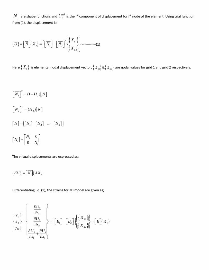
jN are shape functions and 1g
iU is the ith component of displacement for jth node of the element. Using trial function
from (1), the displacement is:
1
1 2
2
g
e
g
XU N X N N
X
------------(1)
Here eX is elemental nodal displacement vector, 1gX & 2gX are nodal values for grid 1 and grid 2 respectively.
1 2
2 2
1 2
(1 )
( )
...
0
0
T
T
n
i
i
i
N H N
N H N
N N N N
NN
N
The virtual displacements are expressed as;
eU N X
Differentiating Eq. (1), the strains for 2D model are given as;
1
1
11
22 1 2
2 212
2 1
1 2
g
e
g
U
x
XUB B B X
x X
U U
x x
Combining the strain displacement matrices of the two grids, modified strain displacement matrix is given by;
1 2
1 2
2 2
1 2
(1 )
... n
B B B
B H B H N
B H B H N
B B B B
For 2D plane stress or plane strain, iB can be defines as;
1
2
2 1
2
1
2
2
2 2
2 1
0
0
0
0
i
ii
i i
N
x
NB
x
N N
x x
H
x
HH
x
H H
x x
Modified weak form for contact implementation can then be written as;
1 2 1 2
1
1 1
e
e t
NE TTe e
e
NE NBET TT Te e
e e
X B B C B B X d
X N b d X N t d
Where NE is number of elements and NBE is number of boundary elements

Contact Problems:
In solid mechanics, contact problems are of two types:
Tied Problems
Contact with sliding Problems
Tied Problems:
In tied problems, two parts contacting each other are fixed and do not slide with respect to each other. In these
problems, we need to compute the contact stresses. To fix these two parts, boundary conditions can be prescribed in
global coordinate system. And there is no need to determine normal to contact surface, between two parts, and all the
boundary conditions can be prescribed using global coordinate system. In other words, irrespective of the orientation of
two parts, it is not required to create a local coordinate system at the contact surface to prescribe essential and natural
boundary conditions. Hence in such problems, no transformation matrix is required. The above discussed theory very
well holds for tied problems. Following is the generalized 3D equations for tied problems, derived based on
aforementioned theory.
Numerical Formulation for displacement in contact modelling in Global coordinate system for tied problem:
Let xH be step function, in X direction, of part 2 and yH be step function, in Y direction, of part 2 and zH be step
function, in Z direction of part 2. So respective step functions in X, Y and Z directions for part 1 are (1 )xH , (1 )yH
and (1 )zH .
1 2
1 1
( *(1 )) ( *( ))n n
g g
i i x i i x
i i
U U N H U N H
1 2
1 1
( *(1 )) ( *( ))n n
g g
i i y i i y
i i
V V N H V N H
1 2
1 1
( *(1 )) ( *( ))n n
g g
i i x i i x
i i
W W N H W N H
1 2
1 1
1 21 11 1
1 21 11 1
1 1
1 0 0 0 0 .. .. 0 0 0 0 .. ..
0 1 0 0 0 .. .. 0 0 0 0 .. ..
0 0 1 0 0 .. .. 0 0 0 0 .. .... ..
.. ..
(1 )
g g
g gx x
g gy yXYZ
z z
x
XYZ
U U
H N H NV V
U H N H NW W
H N H N
H N
U
1 2
1 1
1 21 11 1
1 21 11 1
1 1
0 0 .. .. 0 0 .. ..
0 (1 ) 0 .. .. 0 0 .. ..
0 0 (1 ) .. .. 0 0 .. .... ..
.. ..
g g
g gx
g gy y
z z
U U
H NV V
H N H NW W
H N H N
11
11
11
1 11 1
11
(1 ) 0 0 ..
0 (1 ) 0 ..
0 0 (1 ) ..
(1 ) (1 ) 0 ..
0 (1 )
XX
YY
ZZ
X YX Y
Y
N HUH N
X XX
N HVH N
Y YY
N HWH N
Z Z Z
U V N H N HH N H N
Y X Y Y X X
V W NH N
Z Y Z
W U
X Z
1
1
1
1
1
1
11
1 11 1
6*3
11
11
11
..
..(1 ) ..
(1 ) 0 (1 ) ..
( ) 0 0 ..
0 ( ) 0 ..
0 0 ( ) ..
g
g
g
Y ZZ
X ZX Z
n
XX
YY
ZZ
U
V
W
H N HH N
Z Y Y
N H N HH N H N
Z Z X X
N HH N
X X
N HH N
Y Y
N HH N
Z Z
2
1
2
1
2
1
1 11 1
1 11 1
1 11 1
6*3
( ) ( ) 0 .. ..
..0 ( ) ( ) ..
( ) 0 ( ) ..
g
g
g
X YX Y
Y ZY Z
X ZX Z
n
U
V
WN H N H
H N H NY Y X X
N H N HH N H N
Z Z Y Y
N H N HH N H N
Z Z X X
1
1 22
11
11
11
1
1 11 1
1
(1 ) 0 0 ..
0 (1 ) 0 ..
0 0 (1 ) ..
(1 ) (1 ) 0 ..
0 (1 )
xy
yzg
ixz
gxy i
yz
xz
XX
YY
ZZ
Tied
X YX Y
Y
UStrain B B
U
N HH N
X X
N HH N
Y Y
N HH N
Z ZB
N H N HH N H N
Y Y X X
NH
11 1
1 11 1
6*3
(1 ) ..
(1 ) 0 (1 ) ..
Y ZZ
X ZX Z
n
H N HN H N
Z Z Y Y
N H N HH N H N
Z Z X X

11
11
11
2
1 11 1
1 11 1
1 11 1
( ) 0 0 ..
0 ( ) 0 ..
0 0 ( ) ..
( ) ( ) 0 ..
0 ( ) ( ) ..
( ) 0 ( ) ..
XX
YY
ZZ
Tied
X YX Y
Y ZY Z
X ZX Z
N HH N
X X
N HH N
Y Y
N HH N
Z ZB
N H N HH N H N
Y Y X X
N H N HH N H N
Z Z Y Y
N H N HH N H N
Z Z X X
6*3n
1 2
Tied Tied
TiedB B B
The entire B matrix for tied problems is obtained by concatenating the above two matrices. Once the B matrix is
obtained, TB DB is computed for tied problems.
Contact with Sliding Problems:
These problems differ with tied problems with respect to prescribing boundary conditions. In these problems, one part
can slide along in two dimensions with respect to other part and it is fixed only in one dimension. Normal to contact
surface is computed and two parts are fixed in this normal direction. In other two dimensions perpendicular to this
normal, one part can slide with respect to other part. Depending on the orientation of two parts and hence the contact
surface, it is imperative that local coordinate system must be created with normal to contact surface being Y axis. For 2D
problems, one part can slide in X direction of this local coordinate system and for 3D problems, one part can slide along
X and Z directions of this local coordinate system. Hence the displacement formulation is obtained with respect to this
local coordinate system and therefor it has to be transformed and should be computed with respect to global coordinate
system. Following equations are derived for generalized 3D case along the lines of theory discussed above and equations
are slightly different when compared to tied problems because of transformation matrix.
Contact Modelling – Transformation Implemented:
Numerical Formulation for displacement in contact modelling in Global coordinate system:
Let xH be step function, in X direction, of part 2 and yH be step function, in Y direction, of part 2 and zH be step
function, in Z direction of part 2. So respective step functions in X, Y and Z directions for part 1 will be (1 )xH ,
(1 )yH and (1 )zH .

1 2
1 1
( *(1 )) ( *( ))n n
g g
i i x i i x
i i
U U N H U N H
1 2
1 1
( *(1 )) ( *( ))n n
g g
i i y i i y
i i
V V N H V N H
1 2
1 1
( *(1 )) ( *( ))n n
g g
i i x i i x
i i
W W N H W N H
1 2
1 1 1 1
1 2
1 1 1 1
1 21 11 1
1 0 0 0 0 .. .. 0 0 0 0 .. ..
0 1 0 0 0 .. .. 0 0 0 0 .. ..
0 0 1 0 0 .. .. 0 0 0 0 .. ..
... .....
g g
x x
g g
y y
g gz z
U H N U H N U
V H N V H N V
W H N H NW W
Similar expression can be written for displacement in terms of local coordinate system for contact modelling. The idea
now is to write the displacement formulation in local coordinate, in terms of global coordinate system. For that we need
to plug in suitable transformation matrix and derive the equation accordingly. Following is the theory that states as to
how the right transformation matrix is obtained.
Let the global co-ordinate system be represented by X-Y-Z. Local co-ordinate system is represented by X’-Y’-Z’. Then
the transformation matrix is obtained by:
1 2 3
'
'
'
X X
Y n n n Y
Z Z
Here 1n is the direction cosines of unit vector along 'X . Similarly 2 3&n n are direction cosines of unit vectors
along 'Y and 'Z .
Above equation can also be written as;
1
2
3
'
'
'
T
T
T
nX X
Y n Y
Z Zn
Now each of the direction cosines are further expanded, then following is obtained:

1 11 12 13
2 21 22 23
3 31 32 33
T
T
T
n n n n
n n n n
n n n n
Then transformation matrix to go from local to global is 11 12 13
21 22 23
31 32 33
n n n
T n n n
n n n
So using above transformation matrix, displacement formulation in local coordinate can be written in terms of global
coordinate as:
1
11 21 31 11 12 13 1 1 11 21 31
1
12 22 32 21 22 23 1 1 12 22 3
113 23 33 31 32 33 1 1
1 0 0 0 0 .. ..
0 1 0 0 0 .. ..
0 0 1 0 0 .. ..
....
g
x
g
y
gz
U n n n H n n n N U n n n
V n n n H n n n N V n n n
W n n n H n n n N W
2
11 12 13 1 1
2
2 21 22 23 1 1
213 23 33 31 32 33 1 1
0 0 0 0 .. ..
0 0 0 0 .. ..
0 0 0 0 .. ..
....
g
x
g
y
gz
H n n n N U
H n n n N V
n n n H n n n N W
2 2 2
11 21 31 11 12 21 22 31 32 11 13 21 23 31 33
2 2 2
11 12 21 22 31 32 12 22 32 12 13
(1 ) (1 ) (1 ) (1 ) (1 ) (1 ) (1 ) (1 ) (1 )
(1 ) (1 ) (1 ) (1 ) (1 ) (1 ) (1
x y Z x y Z x y Z
x y Z x y Z
U n H n H n H n n H n n H n n H n n H n n H n n H
V n n H n n H n n H n H n H n H n n
W
1
1 1
1
22 23 32 33 1 1
2 2 2 111 13 21 23 31 33 12 13 22 23 32 33 13 23 33 1 1
0 0 .. ..
) (1 ) (1 ) 0 0 .. ..
(1 ) (1 ) (1 ) (1 ) (1 ) (1 ) (1 ) (1 ) (1 ) 0 0 .. ..
....
g
g
x y Z
gx y Z x y Z x y Z
N U
H n n H n n H N V
n n H n n H n n H n n H n n H n n H n H n H n H N W
2 2 2
11 21 31 11 12 21 22 31 32 11 13 21 23 31 33
2 2 2
11 12 21 22 31 32 12 22 32 12 13 22 23 32 33
11 1
( ) ( ) ( ) ( ) ( ) ( ) ( ) ( ) ( )
( ) ( ) ( ) ( ) ( ) ( ) ( ) ( ) ( )
x y Z x y Z x y Z
x y Z x y Z x y Z
n H n H n H n n H n n H n n H n n H n n H n n H
n n H n n H n n H n H n H n H n n H n n H n n H
n n
2
1 1
2
1 1
2 2 2 23 21 23 31 33 12 13 22 23 32 33 13 23 33 1 1
0 0 .. ..
0 0 .. ..
( ) ( ) ( ) ( ) ( ) ( ) ( ) ( ) ( ) 0 0 .. ..
....
g
g
gx y Z x y Z x y Z
N U
N V
H n n H n n H n n H n n H n n H n H n H n H N W
1 2
1 1
1 * 2
1 1
1 2
1 1
... ...
g g
g g
g g
U U U
V mH V mH V
W W W

11 1 12 1 13 1
21 1 22 1 23 1
31 1 32 1 33 1 3*3
2 2 2
11 11 21 31
12 21 11 12 21 22 31 32
13 31 11 13 21 23 31 33
22
[ (1 ) (1 ) (1 )]
[ (1 ) (1 ) (1 )]
[ (1 ) (1 ) (1 )]
n
x y Z
x y Z
x y Z
H N H N H N
mH H N H N H N
H N H N H N
H n H n H n H
H H n n H n n H n n H
H H n n H n n H n n H
H
2 2 2
12 22 32
23 32 12 13 22 23 32 33
2 2 2
33 13 23 33
[ (1 ) (1 ) (1 )]
[ (1 ) (1 ) (1 )]
[ (1 ) (1 ) (1 )]
x y Z
x y Z
x y Z
n H n H n H
H H n n H n n H n n H
H n H n H n H
* * *
11 1 12 1 13 1
* * * *
21 1 22 1 23 1
* * *
31 1 32 1 33 1 3*3
* 2 2 2
11 11 21 31
* *
12 21 11 12 21 22 31 32
* *
13 31 11 13 21 23 31 33
22
[ ( ) ( ) ( )]
[ ( ) ( ) ( )]
[ ( ) ( ) ( )]
n
x y Z
x y Z
x y Z
H N H N H N
mH H N H N H N
H N H N H N
H n H n H n H
H H n n H n n H n n H
H H n n H n n H n n H
H
* 2 2 2
12 22 32
* *
23 32 12 13 22 23 32 33
* 2 2 2
33 13 23 33
[ ( ) ( ) ( )]
[ ( ) ( ) ( )]
[ ( ) ( ) ( )]
x y Z
x y Z
x y Z
n H n H n H
H H n n H n n H n n H
H n H n H n H
1 2
1 1
1 2
1 1
1 2
1 1
1 2
1 2
1 2
1 2
( ) ( )... ...
g g
g g
g g
s
g g
N N
g g
N N
g g
N N
U
dX
V U U
dY V VW
W WdZ
B BU V
U UdY dX
V VV WW WdZ dY
U W
dZ dX
1
1 22
g
i
sg
i
UB B
U

131 11 1 12 111 1 12 1 13 1
231 21 1 22 121 1 22 1 23 1
31 32 331 1 131 1 32 1 33 1
1
1 11 1 2111 1 21 1
Sliding
HN H N H NH N H N H N
x x x x x x
HN H N H NH N H N H N
y y y y y y
H H HN N NH N H N H N
z z z z z zB
N H N HH N H N
y y x
13 231 12 1 22 1 112 1 22 1 13 1 23 1
31 32 23 331 21 1 1 22 1 1 121 1 31 1 22 1 32 1 23 1 33 1
31131 1 11
H HN H N H N NH N H N H N H N
x y y x x y y x x
H H H HN H N N H N N NH N H N H N H N H N H N
z z y y z z y y z z y y
HN NH N H
x x
32 33 131 11 1 1 12 1 11 32 1 12 1 33 1 13 1
6*3n
H H HH N N H N NN H N H N H N H N
z z x x z z x x z z
** ** * * 131 11 1 12 111 1 12 1 13 1
** ** * * 231 21 1 22 121 1 22 1 23 1
* * ** * *31 32 331 1 131 1 32 1 33 1
2
* 1 111 1
Sliding
HN H N H NH N H N H N
x x x x x x
HN H N H NH N H N H N
y y y y y y
H H HN N NH N H N H N
z z z z z zB
N HH N
y
* ** * * ** * * * *13 231 1 21 1 12 1 21 1 121 1 12 1 22 1 13 1 23 1
* * ** ** * * * *31 32 231 21 1 1 1 22 121 1 31 1 32 1 22 1 23 1
H HN H N H N H N NH N H N H N H N H N
y x x y y x x y y x x
H H HN H N N N H NH N H N H N H N H N
z z y y y y z z z z
** 33133 1
* * * ** ** * * * * *31 32 33 131 1 11 1 1 12 1 131 1 11 1 32 1 12 1 33 1 13 1
6*3n
HNH N
y y
H H H HN N H N N H N NH N H N H N H N H N H N
x x z z x x z z x x z z
' "
1 1 1B B B
1 1 111 12 13
1 1 121 22 23
1 1 131 32 33
'
1
1 1 1 1 1 111 21 12 22 13 23
1 1 1 1 1 121 31 22 32 23 33
1 131 11
N N NH H H
x x x
N N NH H H
y y y
N N NH H H
z z zB
N N N N N NH H H H H H
y x y x y x
N N N N N NH H H H H H
z y z y z y
N NH H H
x z
1 1 1 132 12 33 13
6*3n
N N N NH H H
x z x z

1311 121 1 1
2321 221 1 1
31 32 331 1 1
"
1
13 2311 21 12 221 1 1 1 1 1
31 32 23 3321 221 1 1 1 1 1
31 111 1
HH HN N N
x x x
HH HN N N
y y y
H H HN N N
z z zB
H HH H H HN N N N N N
y x y x y x
H H H HH HN N N N N N
z y z y z y
H HN N N
x z
32 33 13121 1 1 1
6*3n
H H HHN N N
x z x z
Similarly ' "
2 2 2B B B
1 2
Sliding Sliding
slidingB B B
The entire B matrix for contact with sliding problems is obtained by concatenating the above two matrices. Once the B
matrix is obtained, TB DB is computed for sliding problems.
Examples: Tied problems have already been implemented in IBFEM. Sliding has been implemented by using above derivations. To
test the sliding scenario, corresponding examples were created as plane stress, axisymmetric and 3d models and results
were tested. More importantly, in the deformed shape, it was observed if sliding between parts occurred as expected.
Example 1 (Plane Stress) – Sliding parallel to global X direction:
An AISI steel plate of dimensions 0.06m*0.02m *0.01m is contacting another AISI steel plate of dimension
0.06m*0.04m*0.01m. Here downward normal force of 1000N acts on smaller plate and because of Poisson effect this
plate expands in x direction, which is equivalent to sliding in X direction. As expected sliding occurred in X direction
when deformed shape was studied. Material properties for both parts are same. E is 2.0E11 Pa and Poisson ratio is 0.29.
Mesh density is 50*47*1. And elements used are 4 node quadrilateral. Boundary conditions are as shown below.
Because sliding is in X direction, xH is made equal to 1.
Dimensions of plate (in meters):
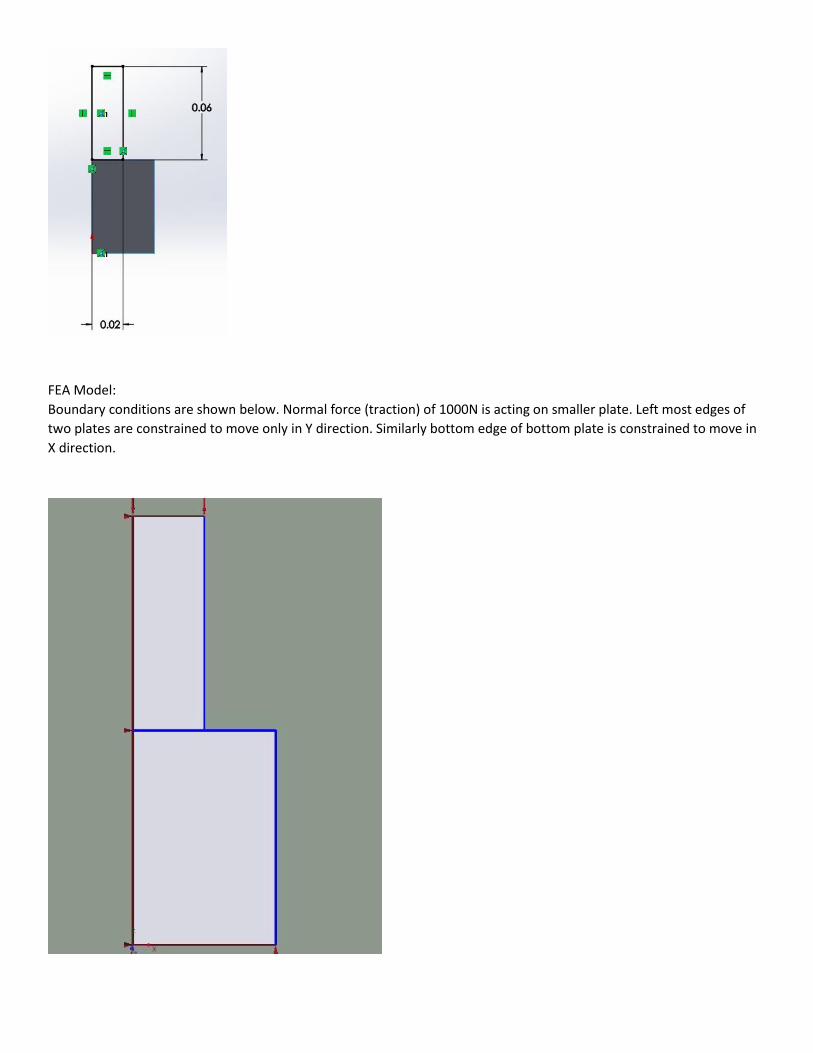
FEA Model:
Boundary conditions are shown below. Normal force (traction) of 1000N is acting on smaller plate. Left most edges of
two plates are constrained to move only in Y direction. Similarly bottom edge of bottom plate is constrained to move in
X direction.

Stress results (Evident that sliding occurs in X direction):
Average stress(green color) on upper plate is found to be 1.115KPa and highest stress (yellow color) is 1.560 KPa.
Displacement Results:
Highest displacement occurs on upper plate and is found to be 5.05E-10 m.
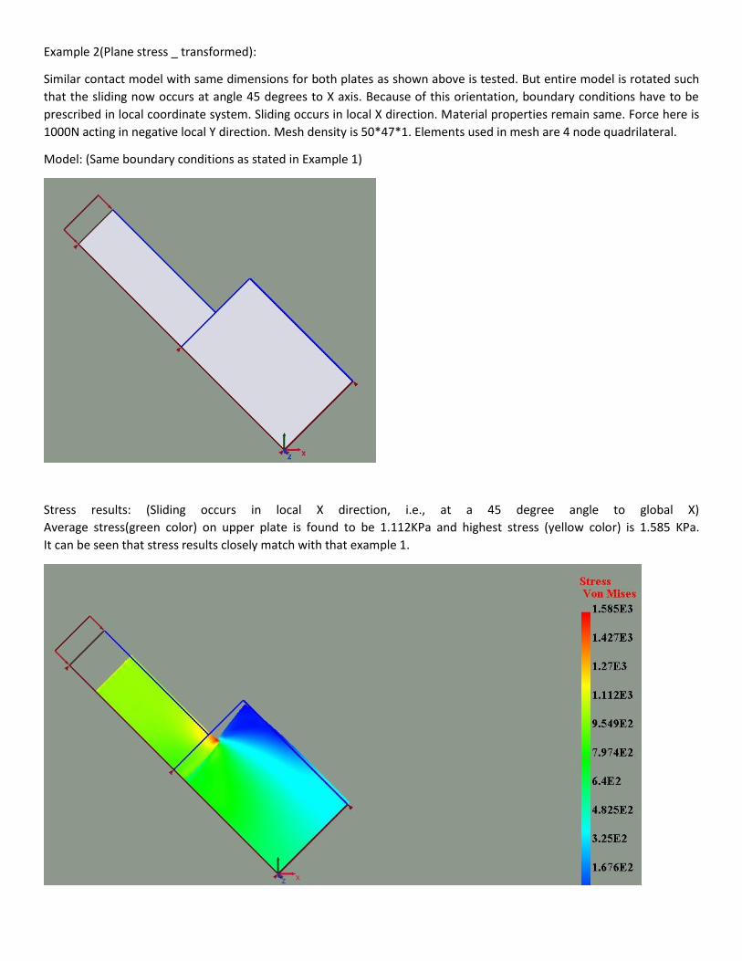
Example 2(Plane stress _ transformed):
Similar contact model with same dimensions for both plates as shown above is tested. But entire model is rotated such
that the sliding now occurs at angle 45 degrees to X axis. Because of this orientation, boundary conditions have to be
prescribed in local coordinate system. Sliding occurs in local X direction. Material properties remain same. Force here is
1000N acting in negative local Y direction. Mesh density is 50*47*1. Elements used in mesh are 4 node quadrilateral.
Model: (Same boundary conditions as stated in Example 1)
Stress results: (Sliding occurs in local X direction, i.e., at a 45 degree angle to global X)
Average stress(green color) on upper plate is found to be 1.112KPa and highest stress (yellow color) is 1.585 KPa.
It can be seen that stress results closely match with that example 1.

Displacement Result:
Highest displacement occurs on upper plate and is found to be 5.05E-10 m. Result exactly matches with that of example
1.
Example 3 (Axisymmetric):
An axisymmetric contact model is created. Actual contact model consists of 2 cones such that slanting surfaces of cones
are contacting each other. This model is modelled as axisymmetric model. When the downward normal force (traction)
of 1000N acts on inner cone, it slides along the slanting surface of outer cone. Sliding occurs along the slanting surface of
the cone. Mesh density used is 30*27*1. Material of both the cones is AISI steel. E is 2.0E11 Pa and Poisson ratio is
0.29.Dimensions of axisymmetric model two cones are shown in following snapshot of the part file. Elements used in
mesh are 4 node quadrilateral.
Dimensions of the Model:

FEA Model:
Boundary conditions are as shown below. Outer cone is fixed and a normal force (traction) of 1000N acts in negative Y
direction on inner cone.

Stress results: (Inner cone deforms along the slanting surface of outer cone and this is what was expected.)
Highest stress is 7.298Kpa found on the inner cone.
Displacement result: Maximum displacement is found to be 1.503E-8 m.

Example 3 is tested again by modifying the mesh density and using 9 node quadrilateral element in the mesh rather than
4 node quadrilateral element. Stress results and displacement results are compared with that of previous analysis. New
mesh density used is 50*47*1.
Stress results: Highest stress observed is 7.679 Kpa. In previous case it was observed to be 7.298Kpa. Finer mesh has
resulted in answer being closer to actual one.
Displacement Results:
Highest displacement is observed to be 1.493E-8m. In previous case it was 1.503E-8m.

Example4(3DModel):
Same model as described in example 3 is recreated as 3D model in example 4. Instead of modelling cones as
axisymmetric, they have been modelled as 3d cones with revolve angle being 90 deg. A downward force of 1000N acts
on inner cone while the outer cone is held fixed. Materials of both cones are AISI steel with E being 2.0E11 Pa and
Poisson ratio being 0.29. Dimensions of sketches used for revolving to obtain 3d models are shown below. Mesh density
used is 11*11*11. Elements used in mesh are 8 node hexahedron.
Dimensions:

FEA Model (Boundary Conditions are as shown below):
But unfortunately analysis could not be performed as mesh could not be generated. Probable reason for this has been
identified in graphics code. While trying to create the mesh, graphics code is crashing. This has to be rectified for the 3d
model to run. So this will be part of the work from here on. In addition to this suitable changes have to be made in
element contact code for the 3d model to run.
Future Work:
So far EBC transformation has been accomplished for plane stress, plane strain. Axisymmetric and 3D models.
This concept was used to implement sliding in contact problems. Sliding has been successfully accomplished in
plane stress and axisymmetric models. Future work from here on will be to make necessary changes in graphics
code to enable mesh generation for 3D model and also to make suitable changes in element contact for 3D to
work. Precisely, the code to find number of contact line triangles has to be modified suitably for 3D model.
With sliding accomplished for all models, next step would be to implement friction and to be precise, coulomb
friction and viscous friction have to be implemented in IBFEM. So when sliding takes place in an assembly,
friction will be taken into account. First step to this will be to read research papers that deal with implementing
friction numerically in meshless techniques.
Also, 3D line contact and 3D point contact type problems with sliding have to be implemented.