CONSUMPTION OVER THE LIFE CYCLE: FACTS FROM …jesusfv/Consumption_Life_Cycle.pdf · cycle consumption patterns with their empirical counter-parts therefore requires removing these

CONSUMPTION OVER THE LIFE CYCLE: FACTS FROM CONSUMEREXPENDITURE SURVEY DATA

Jesus Fernandez-Villaverde and Dirk Krueger*

Abstract—This paper uses Consumer Expenditure Survey data and aseminonparametric statistical model to estimate life cycle profiles ofconsumption, controlling for demographics, cohort, and time effects. Weconstruct age profiles for total and nondurable consumption as well asexpenditure patterns for consumer durables. Special emphasis is placed onthe comparison of different approaches to control for changes in demo-graphics over the life cycle. We find significant humps over the life cyclefor total, nondurable, and durable expenditures. Changes in household sizeaccount for roughly half of these humps. Bootstrap simulations suggestthat our empirical estimates are tight in that standard errors are small.

I. Introduction

THIS paper uses Consumer Expenditure Survey (CEX)data to estimate life cycle profiles of consumption,

controlling for demographics, cohort, and time effects. Inaddition to documenting profiles for total and nondurableconsumption, we provide an age expenditure pattern forconsumer durables.

Two reasons motivate our empirical study. First, we wantto provide empirical life cycle consumption profiles that canbe used to assess the ability of quantitative life cyclesimulation models, pioneered by Auerbach and Kotlikoff(1987), to match the data. These models typically abstractfrom business cycle fluctuations, cohort effects, and differ-ences in household size. Comparing model-generated lifecycle consumption patterns with their empirical counter-parts therefore requires removing these effects. In thispaper, special emphasis is placed on the comparison ofdifferent approaches to control for changes in demographicsover the life cycle.

Second, we report life cycle expenditure patterns forconsumer durables, the most important asset in the medianU.S. household’s wealth portfolio. To the best of our knowl-edge, we are the first to exploit CEX data to construct theseprofiles, which can also be used to evaluate quantitativetheoretical models that incorporate consumer durables. Weundertake the analysis of nondurables and durables jointlysince households’ decisions to purchase nondurables anddurables or to save in financial assets are intertwined by theperiod budget constraint. Furthermore, a household’s abilityto borrow may depend on its stock of consumer durables,pointing to further interdependence between the life cycleprofiles for nondurables and durables. By quantifying the

size, timing, and correlation between the humps in nondu-rables and durables, our empirical results may shed light onwhich elements a successful model must possess to accu-rately account for the data.

Our main result is that total consumption expenditures aswell as expenditures for nondurables and durables display asignificant hump over the life cycle, even after accountingfor changes in family size. If we measure the hump as theratio of peak consumption to consumption at age 22, the sizeof the hump before demographic adjustment is roughly 1.6and 1.3 thereafter. This finding is difficult to reconcile withthe basic version of the life cycle model, augmented withconsumer durables (that is, separable utility between non-durables, durables, and leisure, no adjustment costs, andcomplete markets). The empirical evidence suggests theneed for enriching this model with further elements, such asnonseparabilities in the utility function, different forms ofadjustment costs or indivisibilities for consumer durables,or prudence in the light of idiosyncratic uncertainty.

Our paper builds on the sizable literature documentingempirical life cycle consumption expenditure profiles, ex-amples of which include, among many others, Carroll andSummers (1991), Carroll (1992), Deaton (1992), Kotlikoff(2001), and Gourinchas and Parker (2002). However, itoffers the following new contributions. First, to the best ofour knowledge, we are the first to employ the informationon consumer durables from the Consumer ExpenditureSurvey to build life cycle expenditure profiles of theseitems.

Second, we revisit the issue of controlling for family sizeand propose the use of household equivalence scales for thispurpose. The recent contributions of Blundell, Browning,and Meghir (1994), Attanasio and Browning (1995), andAttanasio et al. (1999) emphasize the importance of changesin household size to rationalize consumption expenditureprofiles over the life cycle. These papers argue that demo-graphics can explain, at least to a substantial degree, whyconsumption tracks income over the life cycle. Using house-hold equivalence scales we find that demographics indeedplay a large role, accounting for roughly half of the size ofthe hump in both expenditures on nondurables and durables.When employing household size adjustments implicitly es-timated by other papers in the consumption life cycleliterature, we document that even with these alternativeadjustment procedures, a sizable hump emerges.

Third, we control for cohort, time, and age effects in aflexible way by employing a seminonparametric partiallylinear model that imposes minimum conditions on the data.This procedure provides efficiency advantages in estimating

Received for publication November 26, 2002. Revision accepted forpublication June 15, 2006.

* University of Pennsylvania; and University of Frankfurt, CEPR, andNBER, respectively.

We would like to thank Andrew Atkeson, Michele Boldrin, Hal Cole,MariaCristina De Nardi, Thesia Garner, Narayana Kocherlakota, LeeOhanian, Luigi Pistaferri, Edward Prescott, participants at seminars innumerous institutions, members of the Bureau of Labor Statistics, andespecially Daron Acemoglu and two referees for many helpful comments,and the NSF under grants SES-0004376 and SES-0234267 for financialsupport. All remaining errors are our own.

The Review of Economics and Statistics, August 2007, 89(3): 552–565© 2007 by the President and Fellows of Harvard College and the Massachusetts Institute of Technology

age profiles compared to the use of dummy variables, yet istractable and relatively straightforward to implement.

Finally, we perform bootstrap simulations to assess theprecision of our estimates, an issue that has received littleattention in the literature. We find that confidence intervalsand bands are tight around our point estimates. This sug-gests that the hump cannot be explained purely by samplinguncertainty. In addition, an extensive sensitivity analysisshows that our main findings survive across a wide set ofeconometric specifications.

The rest of the paper is organized as follows. Section IIdescribes the CEX data. Section III presents the specifica-tion of the estimated model of life cycle consumption. Italso explains in detail how we control for age, time, andcohort effects, and for demographic changes. Section IVdiscusses our empirical findings, with section V evaluatingthe precision of the estimates using the bootstrap. In sectionVI we compare our results with those obtained employingalternative demographic adjustment procedures. Section VIIoffers concluding remarks. Further details about the data,variable definitions, estimation, results, and robustness anal-ysis are contained in a technical appendix, available athttp://www.econ.upenn.edu/˜jesusfv/appen_consum.pdf.

II. The CEX Data

We exploit the 1980–2001 Consumer Expenditure Sur-vey, a widely used source of data on consumption expen-ditures (see Attanasio, 1998). We excluded the years 1982and 1983 because of methodological differences in thesurvey. The CEX is a rotating panel. Each household isinterviewed every three months over five calendar quarters,and every quarter 20% of the sample is replaced by newhouseholds. The CEX is designed to constitute a represen-tative sample of the U.S. population, with a sample size ofabout 5,000 households.

We deflate each expenditure category using its own spe-cific, not seasonally adjusted, consumer price index (CPI)component for urban consumers. The dollar figures areadjusted to 1982–1984 dollars using the “current methods”version of the CPI. This version rebuilds past CPIs with thepresent methodology to produce a price deflator series thatis consistent over time.

For the purpose of this paper, two issues with the way theCEX data are collected make it difficult to use them directly.First, the CEX records data only on consumption expendi-ture, and not on consumption services, our final object ofinterest. Second, the CEX lacks a significant panel dimen-sion since it follows households for at most five quarters. Inthe remaining part of this section we discuss how weaddress both issues.

A. Expenditures versus Consumption

As mentioned before, the CEX does not report a measureof consumption services, arguably the object of strongest

interest from the point of economic theory; it reports onlyexpenditures on consumption goods. This distinction is notvery relevant for the case of nondurable goods, but it iscrucial when dealing with durables. For example, if thehousehold buys a car today, it will receive a flow oftransportation services over a long number of periods,despite the fact that expenditures are incurred (and show upin the data) only in the current period.

However, since data problems prevent us from reliablyimputing services flows from information on the stock ofconsumer durables, we focus our analysis on expendituredata.1 Quantitative life cycle models that incorporate du-rables have predictions not only for service flows fromdurables but also for the timing of expenditures on thesedurables over the life cycle. Our results may serve as anempirical benchmark against which the predictions of thesemodels can be evaluated.2

B. A Pseudopanel Approach

The second problem mentioned above is that the shortpanel dimension of the CEX makes the use of direct paneltechniques problematic. An alternative is to exploit therepeated nature of the survey and build a pseudopanel (seeDeaton, 1985). New households that enter the survey are arandomly chosen large sample of the U.S. population, andconsequently, they contain information about the consump-tion means of the groups they belong to. This informationcan be used by interpreting the observed group means as apanel for estimation purposes. Also, a pseudopanel reducesthe attrition problem, approximately averages out expecta-tional errors, and eliminates the need to control for individ-ual effects since it aggregates across agents.

We use the age of the reference person to associate ahousehold with a cohort. We define ten cohorts with a lengthof five years, evaluate their means using CEX-providedpopulation weights, and follow them through the sample togenerate a balanced panel. Our choice of ten cohorts is acompromise between the need for a large time series di-mension to enrich the longitudinal aspect of the pseudo-panel and the desire for a large cohort size to confidentlyassume that the sample means are good approximations fortheir population counterparts. Most of our cells have be-

1 The CEX provides only partial information for the value of the stockof durables. While the survey asks for an estimate of the current value ofthe owned residence and the original cost of vehicles, it takes only aphysical, but not a value, inventory of major appliances owned by thehousehold. The omission of these items may significantly underestimatethe stock of durables for low-wealth households. Thus, since youngerhouseholds tend to be wealth-poor, the omission may distort estimates oflife cycle consumption profiles for durables. Also, since we do not observethe initial stock of durables of the cohort and the sample length is small,we cannot use the perpetual inventory method to build estimates of thestock of consumer durables.

2 In the technical appendix we exploit the information in the CEX oncurrent values of owned residences, thus indirectly providing life cycleprofiles of services from owned homes. If owner-occupied housing andother durables are complements, life cycle profiles of housing services canserve as first approximations of profiles for other durables.

CONSUMPTION OVER THE LIFE CYCLE 553

tween 200 and 500 observations, and on average, around350.

III. Specification and Estimation of Life Cycle Profiles

The most straightforward way to document consumptionprofiles over the life cycle is to use the pseudopanel to plotconsumption against the age of the household’s head. Thissimple procedure, however, faces two problems. First,households in these cohorts were born at different dates andmay have experienced very different conditions during theirlifetime. With positive long-run growth of real wages, forexample, cohorts born at later dates have higher discountedlifetime earnings. Therefore, it is key to control for cohorteffects. But even if we could observe one cohort over itsentire life cycle, aggregate fluctuations would affect thecohort’s consumption profiles. These effects should be at-tributed to time rather than aging. In subsection IIIA wedescribe how to disentangle cohort and time effects fromage effects, the primary object of interest of our analysis.

Second, the CEX reports consumption data for house-holds and not for individuals. Since we want to provideempirical life cycle consumption patterns to evaluate quan-titative life cycle models, which usually abstract from vari-ations of household composition, it is crucial to separatechanges in expenditures induced by changes in family sizeand changes induced by other factors. We describe insubsection IIIB how we adjust the raw data for demograph-ics.

A. Controlling for Age, Cohort, and Quarter Effects

We propose to relate age and consumption expendituresby a simple and flexible seminonparametric regression. Inparticular, we specify the partially linear model:

cit � �icohorti � �t�t � m�ageit� � εit, (1)

where cit is the cohort i average of log consumption at timet, cohorti is a dummy for each cohort (except the youngestone), �t is a dummy for each quarter, ageit is the age ofcohort i at time t, measured in years, m(ageit) �E(cit�ageit) is a smooth function of ageit, and εit is anindependent, zero mean, random error. The random termcaptures multiplicative measurement error in consumptionexpenditures (since the dependent variable is log consump-tion) as well as unobserved cross-sectional heterogeneity.

This specification consists of two different components, aparametric part that includes cohort and quarter dummies,�icohorti � �t�t, and a nonparametric function of age,m(ageit). This combination of a parametric and nonpara-metric approach achieves a satisfactory balance betweenflexibility and efficiency. A fully nonparametric approach ishopelessly inefficient in a small sample such as the pseu-dopanel from the size of the CEX. A pure parametricapproach with age dummies, on the other hand, delivers anonsmooth consumption profile that is difficult to use as an

empirical benchmark. Furthermore, it is not robust to modelmisspecification problems.

We estimate the partially linear model using the two-stepestimator proposed by Speckman (1988). This estimatorcombines ordinary least squares to estimate the parametriccomponent with a standard kernel-smoothing estimator toestimate the nonparametric component.3

Note that because time, age, and cohort effects are lin-early dependent, it is not possible to separately identifythem without further assumptions.4 Following Deaton(1997), our identification scheme assumes that time effectsare orthogonal to a time trend and that their sum is normal-ized to zero.

B. Controlling for Family Size: Household EquivalenceScales

Households of different size plausibly face different mar-ginal utilities from the same consumption expenditures.Economic theory predicts only that marginal utilities shouldbe equated across time (up to some constant that depends ofthe discount factor and the interest rate) and not expendi-tures per se. Since household size displays a hump over thelife cycle, the hump in consumption may largely be ex-plained by changes in household composition, as argued intwo influential papers by Attanasio and Weber (1995) andAttanasio et al. (1999).

Part of the objective of this paper is to quantify how muchof the change in consumption over the life cycle is ex-plained by demographics. We can attribute changes inexpenditures on particular consumption items as a house-hold ages either to changes in household size or to changesin consumption profiles. By using information on expendi-ture shares of households, one can construct householdequivalence scales, which measure the change in consump-

3 Our estimator is described in detail in the technical appendix. Thenonparametric component is estimated using a Nadaraya-Watson estima-tor with an Epanechnikov kernel. For our benchmark estimates we choose,based on cross-validation, a bandwidth parameter for the kernel of fiveyears. We checked that the results are robust to this choice. Note thatsetting the bandwidth to one year is equivalent to estimating a model withage dummies. Thus, our model nests and generalizes this more traditionalapproach. The technical appendix also reports the estimation under thisage-dummy specification and documents that the main results of the paperremain unchanged.

4 Since we apply a nonlinear transformation to the age variable, time,cohort, and age are not perfectly collinear. However, these variables are sohighly collinear that without further identifying restrictions, we wouldobtain extremely imprecise estimates.

TABLE 1.—DIFFERENT HOUSEHOLD EQUIVALENCE SCALES

FamilySize OECD NAS HHS DOC LM Nelson Mean

1 1 1 1 1 1 1 12 1.70 1.62 1.34 1.28 1.06 1.06 1.343 2.20 2.00 1.68 1.57 1.28 1.17 1.654 2.70 2.36 2.02 2.01 1.47 1.24 1.975 3.20 2.69 2.37 2.37 1.69 1.30 2.27

THE REVIEW OF ECONOMICS AND STATISTICS554

FIGURE 1.—TOTAL EXPENDITURE

20 30 40 50 60 70 80 902000

2500

3000

3500

4000

4500

5000

5500

Age

1982

-84

$

FIGURE 2.—EXPENDITURES: NONDURABLES

20 30 40 50 60 70 80 90800

1000

1200

1400

1600

1800

2000

Age

1982

-84

$


tion expenditures needed to keep the welfare of a familyconstant when its size varies.5

The simplest scale divides total expenditures by thenumber of household members to obtain per capita con-sumption. This scale therefore assumes that a household’stechnology to transform expenditures into consumption ser-vice flows exhibits constant returns to scale. Theory andevidence suggest otherwise. Lazear and Michael (1980)point to three mechanisms through which household sizeaffects the rate of transformation between expenditures andservices (family goods, economies of scale, and comple-mentarities) and present data implying that their quantitativeeffects are important. Their findings suggest that moreelaborate equivalence scales are needed to deflate householdconsumption expenditure by household size.

In this paper we borrow from rich previous work thatexploits detailed information on expenditure shares to con-struct household equivalence scales. This literature docu-ments, first, that economies of scale in household consump-tion exist. Second, opinions differ with respect to their size.

To summarize these differences we present a representa-tive sample of household equivalence scales in table 1 (inwhich, for convenience, we assume the first two members ofthe household to be adults and the rest children). Columns2 to 5 are based on expert evaluations, and columns 6 and7 are econometric estimates based on observed choices.6

Interestingly, the two explicit econometric procedures de-liver the biggest economies of scale.

Since all reported estimates have advantages and draw-backs we choose their mean as our benchmark scale; itcombines simplicity and a relatively conservative stand onthe effect of household size. In section VI we document that

5 Early papers that deflate household consumption expenditure by afunction of family size include Zeldes (1989), who adds adjusted foodrequirements as a regressor in some of his Euler equation estimates, andBlundell et al. (1994), who plot the life cycle path of consumption,deflated by the number of adults plus 0.4 times the number of children inthe household, for U.K. data.

6 These are constructed, respectively, by the OECD (OECD, 1982), thePanel on Poverty and Family Assistance of the National Academy ofSciences (Citro & Michael, 1995), the Department of Health and HumanServices (Federal Register, 1991), the Department of Commerce (U.S.Department of Commerce, 1991), Lazear and Michael (1980), and Nelson(1993). Since the latter estimates scales only for families of size 2 orhigher, to complete the table we took 1.06 as the scale entry for house-holds of size 2 from Lazear and Michael (1980). Beyond the results in thetable, the literature presents a large number of alternative equivalencescales, such as Colosanto, Kapteyn, and van der Gaag (1984), Datzingeret al. (1984), Johnson and Garner (1995), Jorgenson and Slesnick (1987),Garner and de Vos (1995), and Phipps and Garner (1994). These scalesstay within the bounds set by columns 2 and 8 of table 1.

FIGURE 3.—EXPENDITURES: DURABLES

20 30 40 50 60 70 80 90400

600

800

1000

1200

1400

1600

1800

Age

1982

-84

$


FIGURE 4.—TOTAL EXPENDITURE: ADULT EQUIVALENT

20 30 40 50 60 70 80 901800

2000

2200

2400

2600

2800

3000

3200

3400

Age

1982

-84

$

FIGURE 5.—EXPENDITURES: NONDURABLES, ADULT EQUIVALENT

20 30 40 50 60 70 80 90800

850

900

950

1000

1050

1100

1150

1200

1250

1300

Age

1982

-84

$


our main findings are quite robust to changes in the house-hold equivalence scale.7

After choosing this equivalence scale, we take consump-tion expenditure measures Cjt from the CEX for householdj at quarter t, use the demographic information of thehousehold to obtain the equivalence scale esjt, and adjustconsumption to obtain cjt � log(Cjt/esjt). Let cit denote thesynthetic cohort i average of cjt, on which we then estimatethe partially linear model

cit � �icohorti � �t�t � m�ageit� � εit. (2)

IV. Results

In this section we present the results of our estimation.First, we plot life cycle profiles of total expenditure (figure1), expenditures on nondurables (figure 2), and expenditureon durables (figure 3), controlling for cohort and time

effects but not for family size. Total quarterly expendituresfollow a clear hump; they increase from $3,300 at the age of22 to $5,400 at the peak in the late forties, and decreaseafterward. This pattern is well known and has been reportedin the literature (see, for example, the widely cited work byCarroll & Summers, 1991). More interestingly, similarhumps appear if we separately plot nondurable consumptionexpenditure (figure 2) and expenditures on durables (figure3) against the age of the household (see the technicalappendix for our definition of total expenditures and du-rables and nondurables expenditures). The hump in durablesexpenditures is, to the best of our knowledge, a fact that hasnot been documented before. Note that both humps, fordurables and nondurables, are of similar magnitude (theincrease from age 20 to the peak is around 80%) and that thepeak occurs at the same stage in the life cycle, around thelate forties.

To control for changes in demographics we now use theequivalence scale discussed in section III and repeat theestimation of life cycle profiles. Figure 4 plots total expen-diture against household age, with controls for cohort andquarter effects. Two main findings deserve comment. First,comparing figure 4 to figure 1, we see that the size of thehump, measured as the ratio between consumption at thepeak and at the beginning of the life cycle, is reduced byabout 50%. Nevertheless, a sizable hump remains: adjusted

7 The use of equivalence scales to adjust for changes in household sizeis not free of problems. First, family size is endogenous. Second, a welfareanalysis requires to infer unconditional preferences for a demographicstructure and consumption, whereas usually only preferences for goodsconditional on a particular demographic profile are studied. Ferreira,Buse, and Chavas (1998) estimate a model that allows for endogenouschoices in family size and obtain even larger economies of scale thanLazear and Michael (1980). Finally, for equivalence scales to be usedsuccessfully, they should not vary across household income levels.Pendakur (1999) finds that they satisfy this requirement.

FIGURE 6.—EXPENDITURES: DURABLES, ADULT EQUIVALENT

20 30 40 50 60 70 80 90400

500

600

700

800

900

1000

1100

Age

1982

-84

$


quarterly consumption increases from around $2,550 tonearly $3,300 and then decreases to about $1,800. Also thepeak in consumption is postponed, close to age 50.

The quarter effects are small, with the exception ofsignificantly negative values in 1992 and significantly pos-itive values for the quarters in 1984 and in 1997 and 1998.This pattern is plausible as it agrees with standard businesscycle dating. The cohort effects are fairly small as well.Different reasons may explain this finding. The strongperformance of the stock market during the last two de-cades, which especially profited older cohorts, may havecompensated the long-run real wage growth advantage(which was less than stellar in the 1980s and early 1990s) ofyounger cohorts with smaller holdings of financial assets.Also the recent increases in the skill premium may havehelped older (and more skilled cohorts) in comparison with(at the current point of their life cycle) less skilled, youngercohorts.

Figure 5 plots demographics-adjusted expenditures onnondurables. Consumption grows until the fifties and thendeclines, especially around retirement age, suggesting thatsome of these consumption expenditures are related towork. Comparing this figure to figure 2 we also observe a

reduction of the hump of about 50%. Figure 6 plots expen-ditures on consumer durables: yet again, we observe a clearhump, although expenditures are already relatively high atthe beginning of the adult life cycle, owing to first purchasesof durable goods. Interestingly enough, the reduction of thehump is quite similar to the case of nondurables. Thesefigures show that both expenditures on durables and non-durables have very similar patterns and peak at the sametime.

The results in figure 5 show that, even if changes indemographic composition of households can account foraround half of the hump in nondurable consumption andhence are crucial in understanding life cycle profiles, theother half remains to be explained by factors not present inthe standard complete markets life cycle model of consump-tion. The profile in figure 6 is even more difficult toreconcile with this textbook model when we augment it byincluding consumer durables. In addition to complete finan-cial markets, suppose that utility is separable in nondurableconsumption and services from durables, and that the realinterest rate is equal to the time discount factor (which, asthe depreciation rate, is constant over time). Then theoptimal life cycle profile of consumer durables is to imme-

FIGURE 7.—TOTAL EXPENDITURE: ADULT EQUIVALENT, BY EDUCATION GROUPS

20 30 40 50 60 70 80 900.6

0.7

0.8

0.9

1

1.1

1.2

1.3

1.4

1.5

1.6

Age

High Education

Low Education

Benchmark


diately build up the desired stock and to simply replacedepreciation from there on. We do not see anything like thisin the data; rather, the process of durables accumulationappears to be incremental over the life cycle.

Our profile for expenditure on durables is, however,consistent with papers that have documented liquidity con-straints in the purchases of consumption durables (Alessie,Devereux, & Weber, 1997; Attanasio et al., 2000; Barrow &McGranahan, 2000; and Eberly, 1994) and with work argu-ing for the importance of nonseparabilities in the utilityfunction (Attanasio & Weber, 1995).8

To further investigate whether liquidity constraints mayplay a role in generating the humps in figures 4 to 6, weconstruct consumption profiles separately for different ed-ucational groups. We report the profiles for total expenditurein figure 7, where to enhance comparability we have nor-malized the profiles at 1 at age 22. We observe that forlow-education households (high school degree or less),there still emerges a hump, although its size is smaller thanin our full-sample benchmark. For high-education (at leastsome college) households, the profile shows the opposite

features: now the hump is bigger in size than for the fullsample. Due to space constraints we report the graphs fornondurables and durables in the technical appendix. It isinteresting to note that the hump for expenditures on du-rables disappears after demographic adjustment for thelow-education group.

These results suggest that liquidity constraints may playan important role in shaping life cycle consumption profiles.Since high-education households have steeper income pro-files as documented in Attanasio et al. (1999), in the pres-ence of liquidity constraints their consumption profile isexpected to track income and be steeper as well. Our resultsprovide suggestive, albeit indirect (and subject to severalqualifications), evidence for the presence and importance ofliquidity constraints.

To investigate whether nonseparabilities between con-sumption and leisure may explain part of the hump, in thetechnical appendix we compute life cycle profiles of hoursworked in the market sector and discuss their correlationwith consumption. We find that nonseparabilities may ex-plain part of the hump, but that this explanation facesseveral problems to quantitatively account for the size andthe timing of the hump.

Finally, note that the presence of a hump is robust tofurther breakdowns of expenditures. For instance, even

8 The evidence is also qualitatively consistent with the importance ofin-kind intergenerational transfers of durables. However, data from theHealth and Retirement Study suggest that these transfers are fairly small(see Cardia & Ng, 2000).

FIGURE 8.—95% CONFIDENCE BAND

20 30 40 50 60 70 80 901500

2000

2500

3000

3500

Age

1982

-84

$


when plotting adult-equivalent food consumption (a neces-sary good for which a higher degree of smoothing would beexpected), we see a hump.9

V. Using the Bootstrap to Evaluate SamplingUncertainty

Since we want to provide empirical life cycle consump-tion profiles that can serve as a useful benchmark forquantitative work, our profiles should be precisely esti-mated. To assess this precision we use the bootstrap. Eventhough under relatively mild technical conditions the Speck-man estimator is consistent and asymptotically normal, itssmall sample properties tend to be better reflected by thebootstrap than by asymptotic approximations.10 This is es-pecially true at both ends of the age profiles because of the

low number of observations. We implement the bootstrap asfollows. We build 500 new pseudopanels sampling withreplacement from the CEX and using the weights providedby the survey. Then we apply the Speckman estimator toeach of these new data sets. Since the small sample bias ofthe kernel estimator distorts the fitted values of the newestimates and therefore transmits the bias to the computedstandard error, Hall (1992b) suggests choosing a newsmoothing parameter h that implies undersmoothing rela-tive to the point estimate. We carry out this bias-removalstrategy with an undersmoothing factor of 0.8. Note thatthe resulting confidence intervals and bands will not becentered on the point estimates because of this under-smoothing.

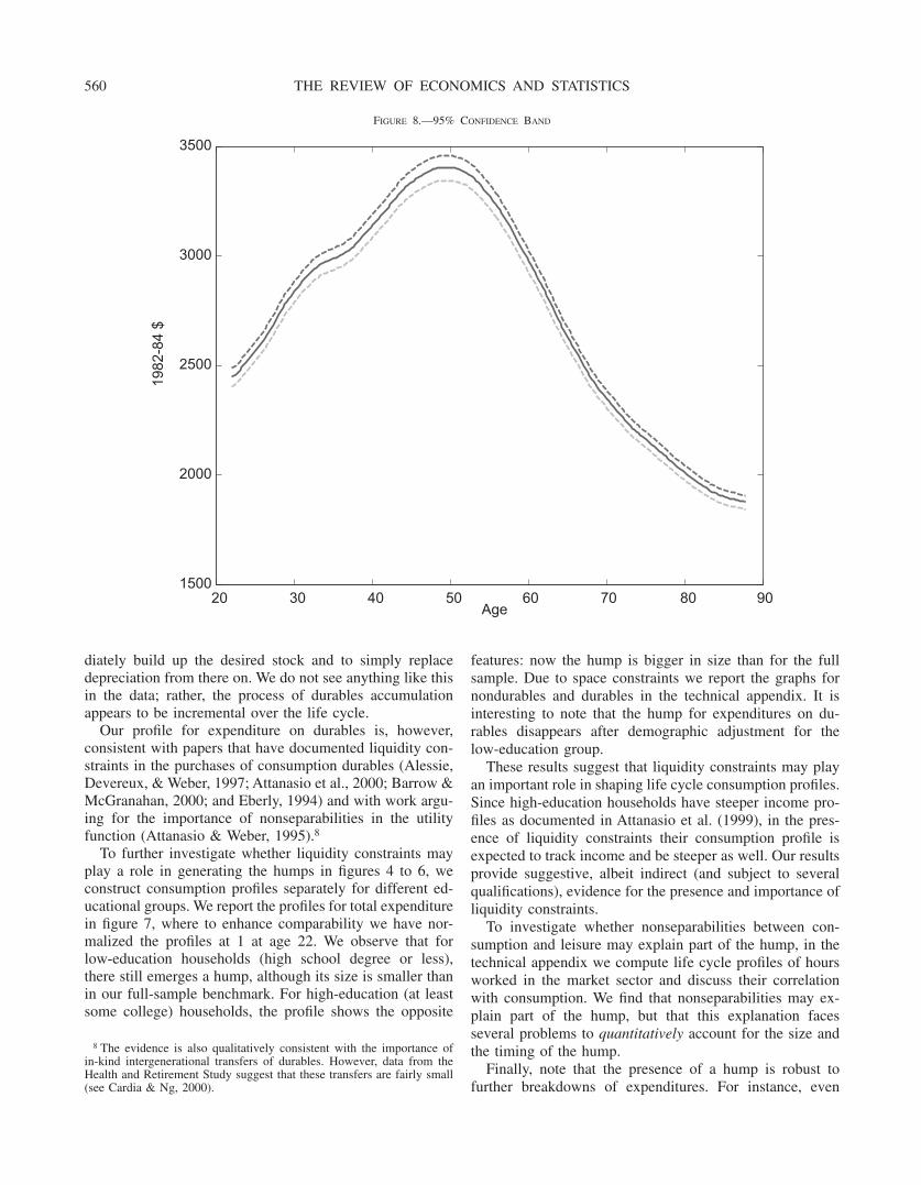
Figure 8 plots a 95% confidence band that covers thewhole true curve (instead of each point separately, as in aconfidence interval). Since any curve that can be plottedentirely inside this small band implies a significant hump,figure 8 strongly reinforces our confidence in the pointestimates: the data indicate a hump in consumption ofnondurables, with size between 20% and 65% and a peakbetween ages 45 and 50. Figure 9 plots all 500 simulatedprofiles: without exception, all simulations generate a quan-titatively significant hump in consumption life cycle pro-

9 Studying food consumption is interesting because it allows comparisonwith data from the Panel Study of Income Dynamics (PSID), a surveywith a long panel dimension. This comparison is performed in Fisher andJohnson (2002), who show that data on food consumption from the PSIDand the CEX agree on the presence and quantitative size of a hump overthe life cycle. The technical appendix offers further information, includinga discussion of the role of housing.

10 The kernel estimates converge more slowly than n�1/ 2 and the asymp-totic distributions have unconventional expansions that are not powers ofn�1/ 2, making their use in finite samples difficult (Hall, 1992a).

FIGURE 9.—ALL SIMULATIONS

20 30 40 50 60 70 80 901500

2000

2500

3000

3500

Age

1982

-84

$


files. Similar results are reported in the technical appendixfor expenditures on nondurables and durables. In all cases,the bootstrap strongly suggests that our findings are notmerely a result of sampling uncertainty.

VI. Comparison with Alternative Procedures

Controlling for changes in household size reduces theconsumption hump by 50%. We now ask how robust thisdecomposition is and if alternative procedures proposed inthe literature result in a complete removal of the hump viachanges in household composition.

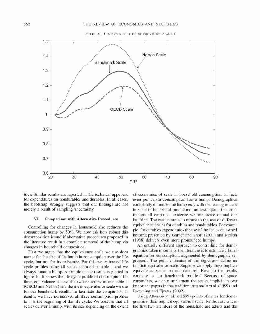
First we argue that the equivalence scale we use doesmatter for the size of the hump in consumption over the lifecycle, but not for its existence. For this we estimated lifecycle profiles using all scales reported in table 1 and wealways found a hump. A sample of the results is plotted infigure 10. It shows the life cycle profile of consumption forthree equivalence scales: the two extremes in our table 1(OECD and Nelson) and the mean equivalence scale we usefor our benchmark results. To facilitate the comparison ofresults, we have normalized all three consumption profilesto 1 at the beginning of the life cycle. We observe that allscales deliver a hump, with its size depending on the extent

of economies of scale in household consumption. In fact,even per capita consumption has a hump. Demographicscompletely eliminate the hump only with decreasing returnsto scale in household production, an assumption that con-tradicts all empirical evidence we are aware of and ourintuition. The results are also robust to the use of differentequivalence scales for durables and nondurables. For exam-ple, for durables expenditures the use of the scales on ownedhousing presented by Garner and Short (2001) and Nelson(1988) delivers even more pronounced humps.

An entirely different approach to controlling for demo-graphics taken in some of the literature is to estimate a Eulerequation for consumption, augmented by demographic re-gressors. The point estimates of the regressors define animplicit equivalence scale. Suppose we apply these implicitequivalence scales on our data set. How do the resultscompare to our benchmark profiles? Because of spaceconstraints, we only implement the scales implicit in twoimportant papers in this tradition: Attanasio et al. (1999) andBrowning and Ejrnæs (2002).

Using Attanasio et al.’s (1999) point estimates for demo-graphics, their implicit equivalence scale, for the case wherethe first two members of the household are adults and the

FIGURE 10.—COMPARISON OF DIFFERENT EQUIVALENCE SCALES I

20 30 40 50 60 70 80 900.6

0.7

0.8

0.9

1

1.1

1.2

1.3

1.4

1.5

Age

Nelson Scale

OECD Scale

Benchmark Scale


rest are children of age less than 16, is {1, 1.57, 1.80, 2.04,2.28}. Of course, different family structures lead to alterna-tive equivalence scales. This scale is quite similar to the onewe employed, although ours implies more economies ofscale for couples: 1.34 versus 1.57 (remember the interpre-tation of household equivalence scales: two persons need$1.34 to obtain the same level of utility as one person livingalone with $1). For bigger families both equivalence scalesindicate roughly the same magnitude of economies ofscales.

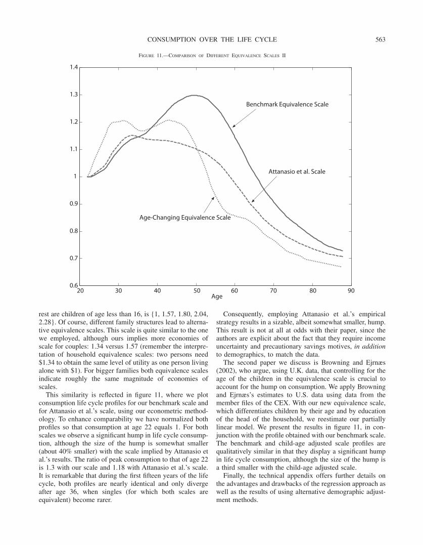
This similarity is reflected in figure 11, where we plotconsumption life cycle profiles for our benchmark scale andfor Attanasio et al.’s scale, using our econometric method-ology. To enhance comparability we have normalized bothprofiles so that consumption at age 22 equals 1. For bothscales we observe a significant hump in life cycle consump-tion, although the size of the hump is somewhat smaller(about 40% smaller) with the scale implied by Attanasio etal.’s results. The ratio of peak consumption to that of age 22is 1.3 with our scale and 1.18 with Attanasio et al.’s scale.It is remarkable that during the first fifteen years of the lifecycle, both profiles are nearly identical and only divergeafter age 36, when singles (for which both scales areequivalent) become rarer.

Consequently, employing Attanasio et al.’s empiricalstrategy results in a sizable, albeit somewhat smaller, hump.This result is not at all at odds with their paper, since theauthors are explicit about the fact that they require incomeuncertainty and precautionary savings motives, in additionto demographics, to match the data.

The second paper we discuss is Browning and Ejrnæs(2002), who argue, using U.K. data, that controlling for theage of the children in the equivalence scale is crucial toaccount for the hump on consumption. We apply Browningand Ejrnæs’s estimates to U.S. data using data from themember files of the CEX. With our new equivalence scale,which differentiates children by their age and by educationof the head of the household, we reestimate our partiallylinear model. We present the results in figure 11, in con-junction with the profile obtained with our benchmark scale.The benchmark and child-age adjusted scale profiles arequalitatively similar in that they display a significant humpin life cycle consumption, although the size of the hump isa third smaller with the child-age adjusted scale.

Finally, the technical appendix offers further details onthe advantages and drawbacks of the regression approach aswell as the results of using alternative demographic adjust-ment methods.

FIGURE 11.—COMPARISON OF DIFFERENT EQUIVALENCE SCALES II

20 30 40 50 60 70 80 900.6

0.7

0.8

0.9

1

1.1

1.2

1.3

1.4

Age

Benchmark Equivalence Scale

Attanasio et al. Scale

Age-Changing Equivalence Scale


VII. Conclusions

In this paper we document the life cycle profiles ofconsumption, with special emphasis on the distinction be-tween expenditures on durables and nondurables. We findthat both expenditures on nondurables and durables have asizable hump, roughly 50% of which is accounted for bychanges in household demographics. The other half remainsto be explained by factors not present in the standardcomplete markets life cycle model of consumption, one ofthe main workhorses of modern macroeconomics. The fail-ure of this textbook model is especially serious for expen-ditures on durables. Instead of immediately building up theirstock of durables and then just compensating for deprecia-tion, households in our data continue to increase expendi-tures until quite late in their life cycles.

A number of possible deviations from the basic life cyclemodel may qualitatively account for the humps documentedin this paper. First, one may relax the assumption of sepa-rability between leisure and consumption. A second depar-ture is the introduction of uninsurable idiosyncratic uncer-tainty (for example, with respect to labor income or lifetimehorizon) into a model where households are prudent. Fi-nally, one may argue for the importance of liquidity con-straints that prevent young households from borrowingagainst future (higher) labor income to finance higher cur-rent consumption. These features, in conjunction with non-convex adjustment costs and indivisibilities for consumerdurables, may help to rationalize the empirical consumptionprofiles we have documented in this paper.

Given the similar timing and size in the humps forexpenditures on nondurables and durables, a successfulmodel will likely incorporate consumer durables intostandard consumption models for nondurables. Examplesof attempts to construct those models and to derive theirquantitative implications include Dıaz and Luengo-Prado(2002), Fernandez-Villaverde and Krueger (2002), andLaibson, Repetto, and Tobacman (2001).

REFERENCES

Alessie, R., M. Devereux, and G. Weber, “Intertemporal Consumption,Durables and Liquidity Constraints: A Cohort Analysis,” EuropeanEconomic Review 41 (1997), 37–59.

Attanasio, O., “Cohort Analysis of Saving Behavior by U.S. Households,”Journal of Human Resources 33 (1998), 575–609.

Attanasio, O., J. Banks, C. Meghir, and G. Weber, “Humps and Bumps inLifetime Consumption,” Journal of Business and Economics 17(1999), 22–35.

Attanasio, O., and M. Browning, “Consumption over the Life Cycle andover the Business Cycle,” American Economic Review 85 (1995),1118–1137.

Attanasio, O., P. Goldberg, and E. Kyriazidou, “Credit Constraints in theMarket for Consumer Durables: Evidence from Microdata on CarLoans,” NBER working paper 7694 (2000).

Attanasio, O., and G. Weber, “Is Consumption Growth Consistent withIntertemporal Optimization? Evidence for the Consumer Expendi-ture Survey,” Journal of Political Economy 103 (1995), 1121–1157.

Auerbach, A., and L. Kotlikoff, Dynamic Fiscal Policy (New York:Cambridge University Press, 1987).

Barrow, L., and L. McGranahan, “The Effects of the Earned IncomeCredit on the Seasonality of Household Expenditures,” NationalTax Journal 53 (2000), 1211–1244.

Blundell, R., M. Browning, and C. Meghir, “Consumer Demand and theLife-Cycle Allocation of Household Expenditures,” Review ofEconomic Studies 61 (1994), 57–80.

Browning, M., and M. Ejrnæs, “Consumption and Children,” Institute ofEconomics, University of Copenhagen, mimeograph (2002).

Cardia, E., and S. Ng, “How Important are Intergenerational Transfers ofTime? A Macroeconomic Analysis,” Johns Hopkins Universitymimeograph (2000).

Carroll, C., “The Buffer-Stock Theory of Saving: Some MacroeconomicEvidence,” Brookings Papers on Economic Activity 23 (1992),61–156.

Carroll, C., and L. Summers, “Consumption Growth Parallels IncomeGrowth: Some New Evidence,” in D. Bernheim and J. Shoven(Eds.), National Saving and Economic Performance (University ofChicago Press for the NBER, 1991).

Citro, C., and R. Michael, Measuring Poverty: A New Approach (NationalAcademy Press, 1995).

Colosanto, D., A. Kapteyn, and J. van der Gaag, “Two SubjectiveMeasures of Poverty. Results from the Wisconsin Basic NeedsSurvey,” Journal of Human Resources 19 (1984), 127–137.

Datzinger, S., J. van der Gaag, M. Taussig, and E. Smolensky, “The DirectMeasurement of Welfare Levels: How Much Does It Cost to MakeEnds Meet?” this REVIEW 66 (1994), 500–505.

Deaton, A., “Panel Data from Time Series of Cross-Sections,” Journal ofEconometrics 30 (1985), 109–126.

Understanding Consumption (Oxford: Oxford University Press,1992).

The Analysis of Household Surveys (Johns Hopkins University,1997).

Dıaz, A., and M. Luengo-Prado, “Durable Goods and the Wealth Distri-bution,” Universidad Carlos III mimeograph (2002).

Eberly, J., “Adjustment of Consumers’ Durables Stocks: Evidence fromAutomobile Purchases,” Journal of Political Economy 102 (1994),403–436.

Federal Register 56, n 34 (1991).Fernandez-Villaverde, J., and D. Krueger, “Consumption and Saving over

the Life Cycle: How Important Are Consumer Durables?” Univer-sity of Pennsylvania mimeograph (2002), available at www.econ.upenn.edu/˜jesusfv.

Ferreira, M., R. Buse, and J. Chavas, “Is There Bias in ComputingHousehold Equivalence Measures?” Review of Income and Wealth44 (1998), 183–198.

Fisher, J., and D. Johnson, “Consumption Mobility in the United States:Evidence from Two Panel Data Sets,” Bureau of Labor Statisticsmimeograph (2002).

Garner, T., and K. de Vos, “Income Sufficiency vs. Poverty: Results fromthe United States and The Netherlands,” Journal of PopulationEconomics 8 (1995), 117–134.

Garner, T., and K. Short, “Owner-Occupied Shelter in ExperimentalPoverty Measurement with a ‘Look’ at Inequality and PovertyRates,” Bureau of Labor Statistics mimeograph (2001).

Gourinchas, P., and J. Parker, “Consumption over the Life Cycle,” Econo-metrica 70 (2002), 47–89.

Hall, P., The Bootstrap and Edgeworth Expansion (New York: Springer-Verlag, 1992a).

“Effect of Bias Estimation on Coverage Accuracy of BootstrapConfidence Intervals for a Probability Density,” Annals of Statistics20 (1992b), 675–694.

Johnson, D., and T. Garner, “Unique Equivalence Scales: Estimation andImplications for Distributional Analysis,” Journal of Income Dis-tribution 4 (1995), 215–234.

Jorgenson, D., and D. Slesnick, “Aggregate Consumer Behavior andHousehold Equivalence Scales,” Journal of Business Economicsand Statistics 5 (1987), 219–232.

Kotlikoff, L., Essays on Saving, Bequest, Altruism and Life-Cycle Plan-ning (MIT Press, 2001).

Laibson, D., A. Repetto, and J. Tobacman, “A Debt Puzzle,” HarvardUniversity mimeograph (2001).

Lazear, E., and Michael, R., “Family Size and the Distribution of RealPer Capita Income,” American Economic Review 70 (1980),91–107.


Nelson, J., “Household Economies of Scale in Consumption: Theory andEvidence,” Econometrica 56 (1988), 1301–1314.

“Independent of a Base Equivalence Scales Estimation UsingUnited States Micro-Data,” Annales d’Economie et de Statistique29 (1993), 43–62.

Organization for Economic Cooperation and Development, The OECDList of Social Indicators (1982).

Pendakur, K., “Semiparametric Estimates and Test of Base-IndependentEquivalence Scales,” Journal of Econometrics 88 (1999), 1–40.

Phipps, S., and T. Garner, “Are Equivalent Scales the Same for the UnitedStates and Canada?” Review of Income and Wealth 40 (1994),1–17.

Speckman, P., “Kernel Smoothing in Partial Linear Models,” Journal ofthe Royal Statistical Society B 50 (1988), 413–436.

U.S. Department of Commerce, Trends in Relative Income: 1964 to 1989,series P60–177 (1991).

Zeldes, S., “Consumption and Liquidity Constraints: An Empirical Inves-tigation,” Journal of Political Economy 97 (1989), 305–346.


Documents

CONSUMPTION OVER THE LIFE CYCLE: FACTS FROM …jesusfv/Consumption_Life_Cycle.pdf · cycle consumption patterns with their empirical counter-parts therefore requires removing these