Consumers’ preferences

ECO61Udayan Roy

Fall 2008

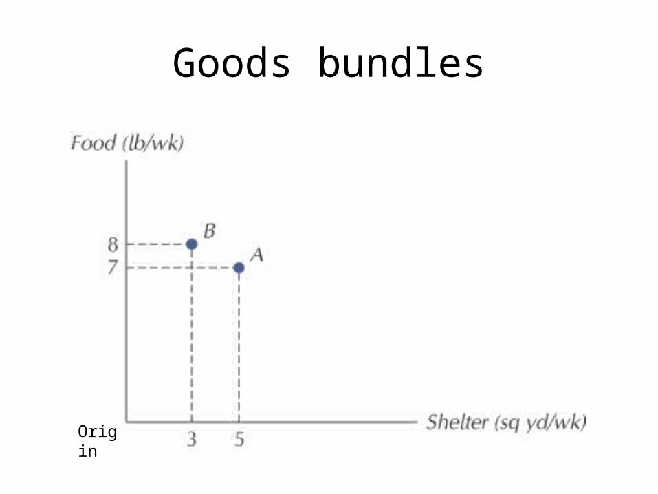
Goods bundles

Origin

Preferences

• Consumers have preferences that they can use to compare different goods bundles

• The preferences may be over goods bundles consumed by oneself or over goods bundles consumed by someone else– For example, a parent may have preferences over

various bundles of food and clothing bought by the parent but consumed by a child

Assumptions about Preference Orderings

• Completeness: the consumer is able to rank all possible bundles of goods and services.– For any two bundles A and B, the consumer knows

whether A is better, or B is better, or they are equally good

• Transitivity: for any three bundles A, B, and C, if A is at least as good as B and B is at least as good as C, then A is at least as good as C.

• These two assumptions imply the ranking principle

The Ranking Principle

• A consumer can rank, in order of preference, all potentially available alternatives

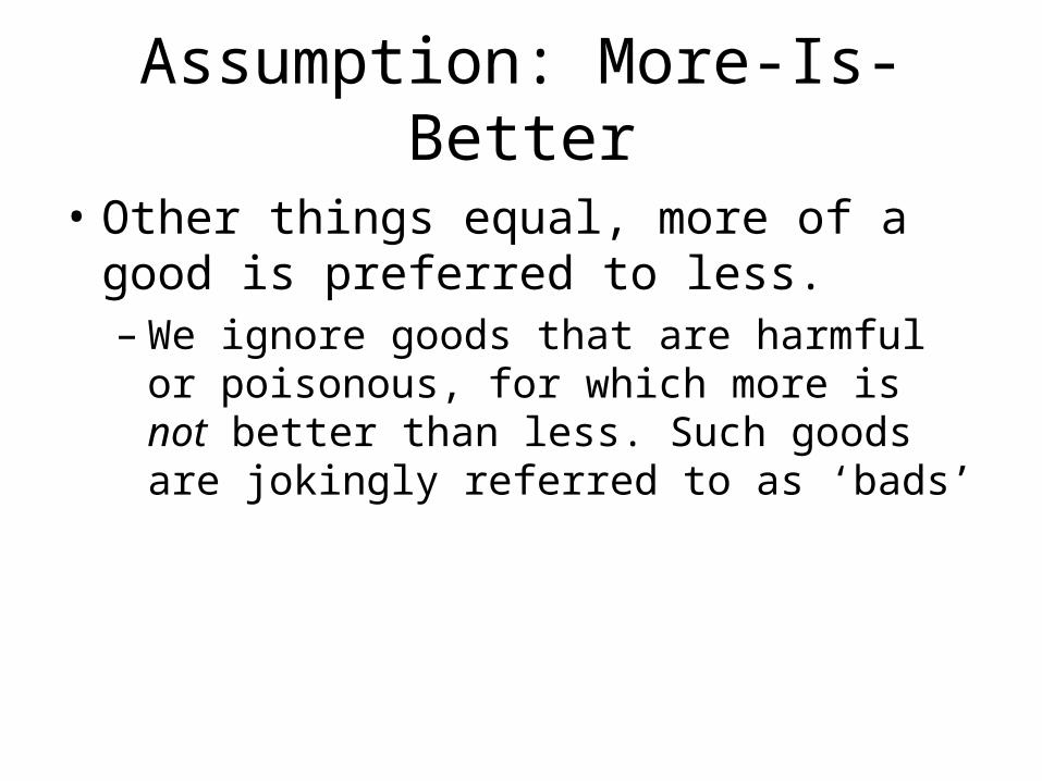
Assumption: More-Is-Better

• Other things equal, more of a good is preferred to less.– We ignore goods that are harmful or poisonous,

for which more is not better than less. Such goods are jokingly referred to as ‘bads’

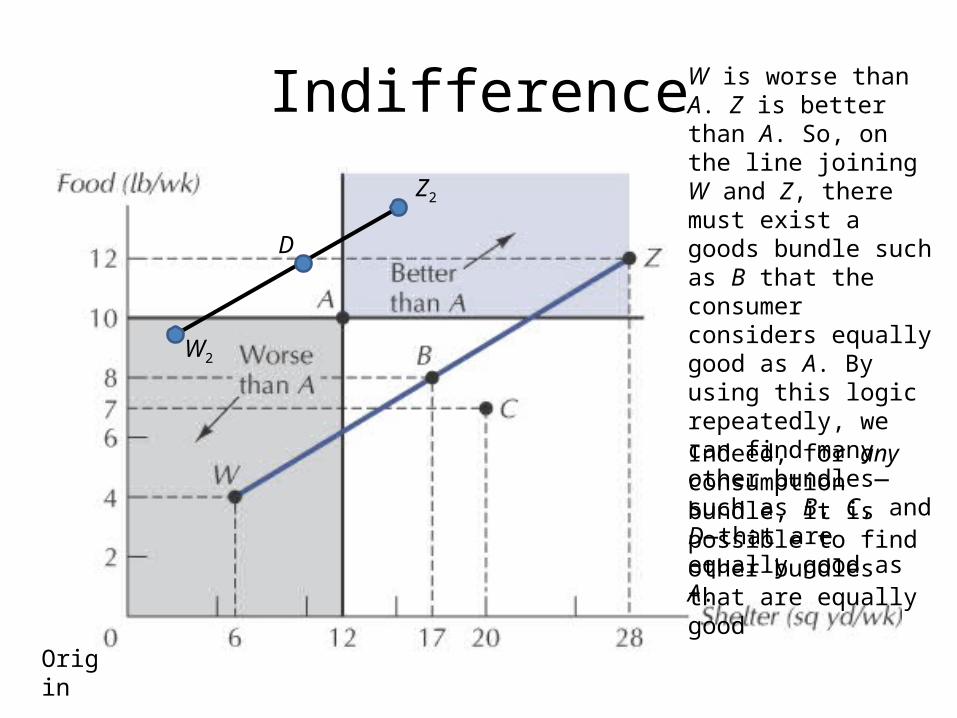
Indifference

Indeed, for any consumption bundle, it is possible to find other bundles that are equally good

Origin

W is worse than A. Z is better than A. So, on the line joining W and Z, there must exist a goods bundle such as B that the consumer considers equally good as A. By using this logic repeatedly, we can find many other bundles—such as B, C, and D—that are equally good as A.

W2

Z2

D

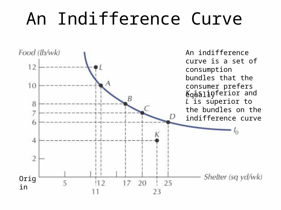
An Indifference Curve

An indifference curve is a set of consumption bundles that the consumer prefers equally

Origin

K is inferior and L is superior to the bundles on the indifference curve

Part of an Indifference Map

Origin

Properties of Indifference Maps

1. Bundles on indifference curves farther from the origin are preferred to those on indifference curves closer to the origin.

2. There is an indifference curve through every possible bundle.

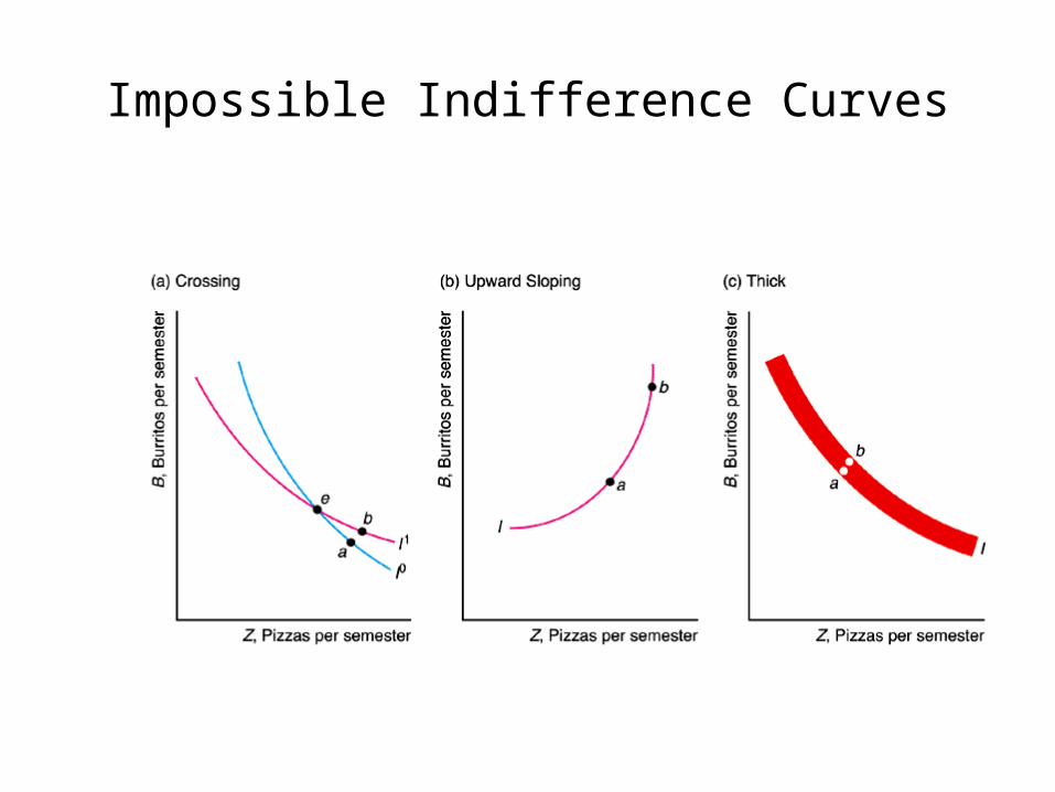
3. Indifference curves cannot cross.4. Indifference curves slope downward.

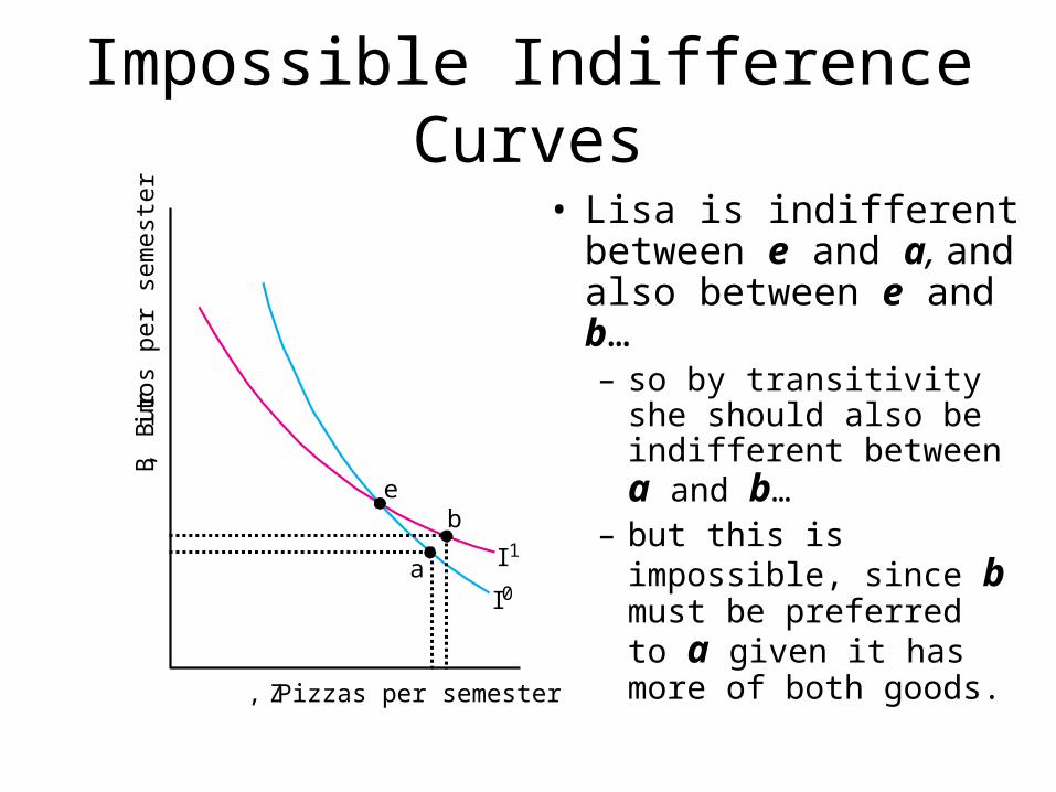
Impossible Indifference Curves

• Lisa is indifferent between e and a, and also between e and b…– so by transitivity she

should also be indifferent between a and b…

– but this is impossible, since b must be preferred to a given it has more of both goods.

B, B

urr

itos

per

sem

est

er

Z, Pizzas per semester

I1

I0a

be

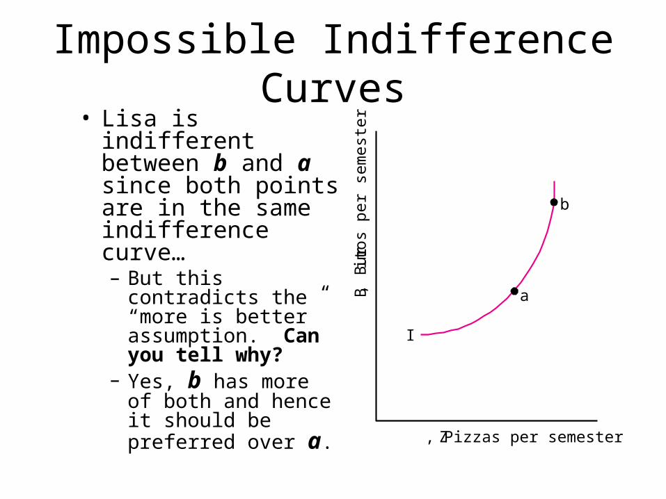
Impossible Indifference Curves• Lisa is indifferent

between b and a since both points are in the same indifference curve…– But this contradicts

the “more is better” assumption. Can you tell why?

– Yes, b has more of both and hence it should be preferred over a.

B, B

urr

itos

per

sem

est

er

Z, Pizzas per semester

I

a

b

Impossible Indifference Curves

Substitution Between Goods

• Economic decisions involve trade-offs• Indifference curves provide information on

the amount of one good that the consumer is willing to give up to gain a unit of another good

4-14

Rates of Substitution

• Consider moving along an indifference curve, from one bundle to another

• This is the same as taking away units of one good and compensating the consumer for the loss by adding units of another good

• Slope of the indifference curve shows how much of the second good is needed to make up for a loss of the first good

4-15

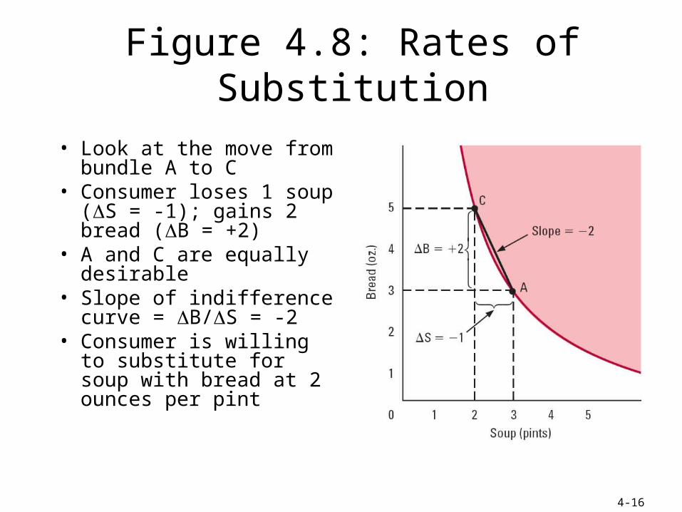
Figure 4.8: Rates of Substitution

• Look at the move from bundle A to C

• Consumer loses 1 soup (S = -1); gains 2 bread (B = +2)

• A and C are equally desirable

• Slope of indifference curve = B/S = -2

• Consumer is willing to substitute for soup with bread at 2 ounces per pint

4-16

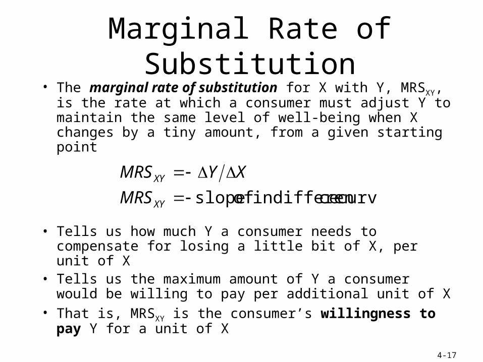
Marginal Rate of Substitution• The marginal rate of substitution for X with Y, MRSXY, is the

rate at which a consumer must adjust Y to maintain the same level of well-being when X changes by a tiny amount, from a given starting point

• Tells us how much Y a consumer needs to compensate for losing a little bit of X, per unit of X

• Tells us the maximum amount of Y a consumer would be willing to pay per additional unit of X

• That is, MRSXY is the consumer’s willingness to pay Y for a unit of X

curve ceindifferen of slope

XY

XY

MRS

XYMRS

4-17

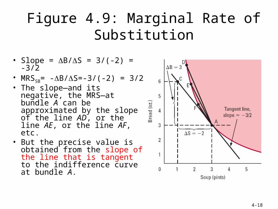
Figure 4.9: Marginal Rate of Substitution

• Slope = B/S = 3/(-2) = -3/2

• MRSSB= -B/S=-3/(-2) = 3/2• The slope—and its negative, the

MRS—at bundle A can be approximated by the slope of the line AD, or the line AE, or the line AF, etc.

• But the precise value is obtained from the slope of the line that is tangent to the indifference curve at bundle A.

4-18

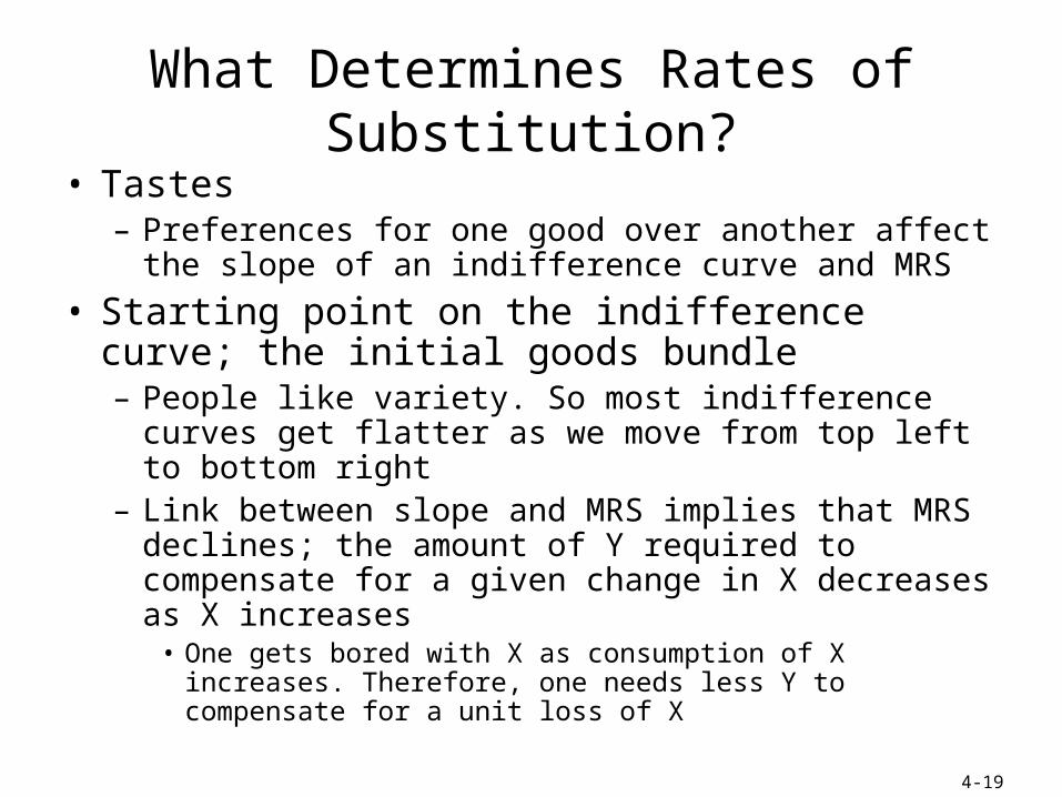
What Determines Rates of Substitution?• Tastes

– Preferences for one good over another affect the slope of an indifference curve and MRS

• Starting point on the indifference curve; the initial goods bundle– People like variety. So most indifference curves get flatter

as we move from top left to bottom right– Link between slope and MRS implies that MRS declines;

the amount of Y required to compensate for a given change in X decreases as X increases

• One gets bored with X as consumption of X increases. Therefore, one needs less Y to compensate for a unit loss of X

4-19

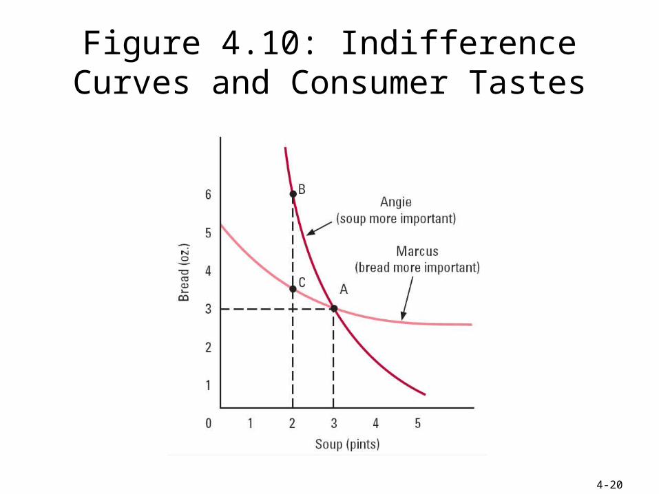
Figure 4.10: Indifference Curves and Consumer Tastes

4-20

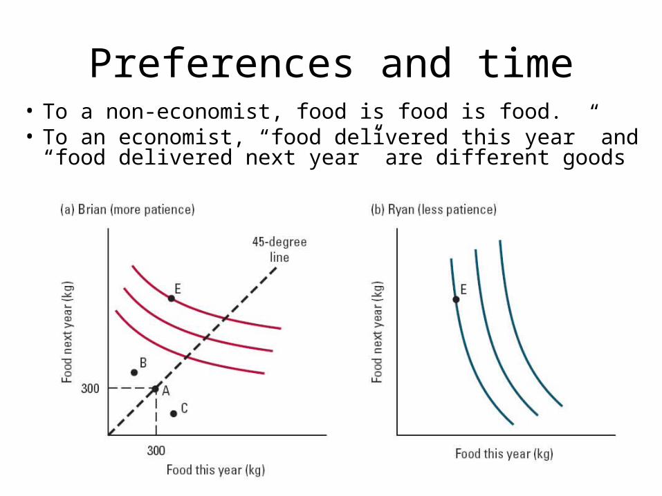
Preferences and time• To a non-economist, food is food is food.• To an economist, “food delivered this year” and

“food delivered next year” are different goods

Preferences and chance• To an economist, “food delivered tomorrow if

it is sunny” and “food delivered tomorrow if there is a hurricane” are different goods

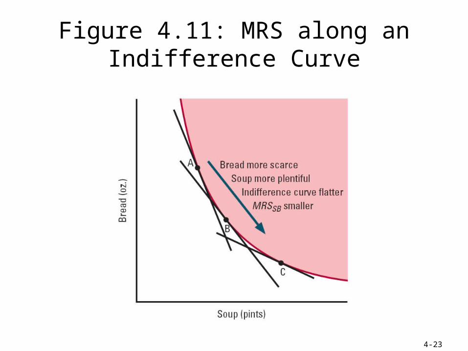
Figure 4.11: MRS along an Indifference Curve

4-23

Perfect Substitutes and Complements

• Two products are perfect substitutes if their functions are identical; in such a case, a consumer is willing to swap one for the other at a fixed rate

• Two products are perfect complements if they are valuable only when used together in fixed proportions

4-24

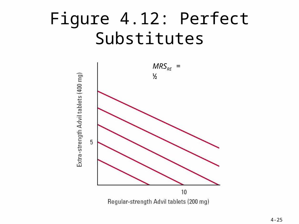
Figure 4.12: Perfect Substitutes

4-25

MRSRE = ½

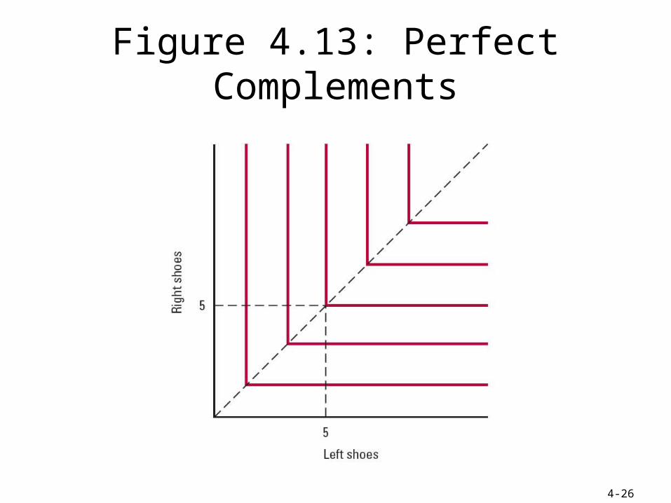
Figure 4.13: Perfect Complements

4-26

Utility

• Recall that under the completeness and transitivity assumptions, the ranking principle is true: – the consumer can rank all bundles according to her

preference• Therefore, the consumer can assign a number to

each bundle such that the numbers assigned to the bundles represent the consumer’s preferences

• The number assigned to a bundle is called its utility

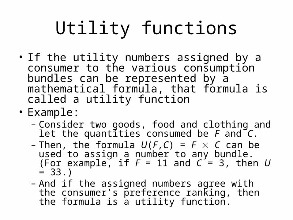
Utility functions• If the utility numbers assigned by a consumer to

the various consumption bundles can be represented by a mathematical formula, that formula is called a utility function

• Example: – Consider two goods, food and clothing and let the

quantities consumed be F and C. – Then, the formula U(F,C) = F C can be used to assign

a number to any bundle. (For example, if F = 11 and C = 3, then U = 33.)

– And if the assigned numbers agree with the consumer’s preference ranking, then the formula is a utility function.

CONSUMER PREFERENCES

A utility function can be represented by a set of indifference curves, each with a numerical indicator.

This figure shows three indifference curves (with utility levels of 25, 50, and 100, respectively) associated with the utility function:

• Utility and Utility Functions

● utility Numerical score representing the satisfaction that a consumer gets from a given market basket.

● utility function Formula that assigns a level of utility to individual market baskets.

Utility Functions and Indifference Curves

u(F,C) = FC

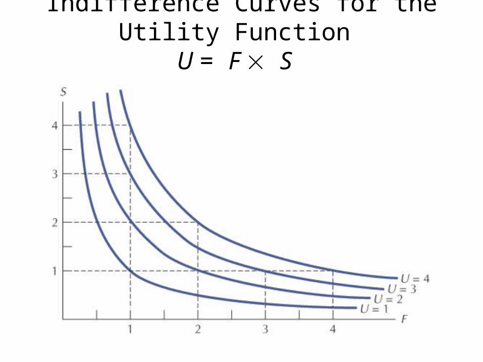
Indifference Curves for the Utility Function U = F S

Marginal Utility

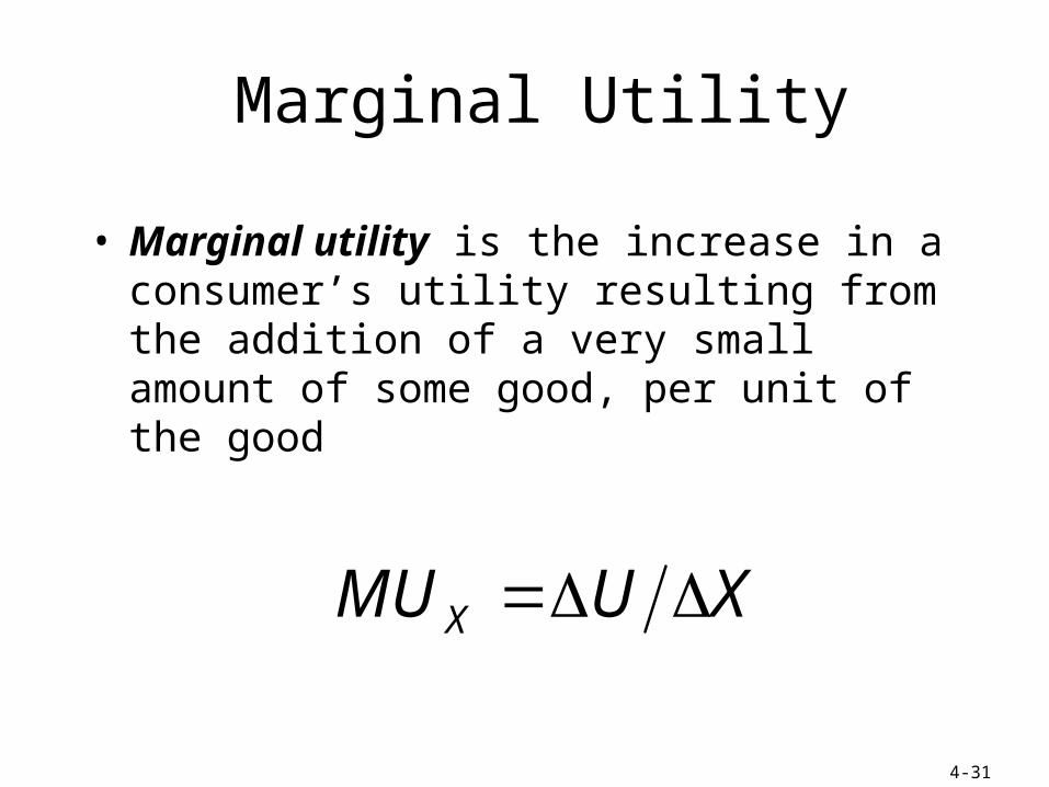
• Marginal utility is the increase in a consumer’s utility resulting from the addition of a very small amount of some good, per unit of the good

XUMU X

4-31

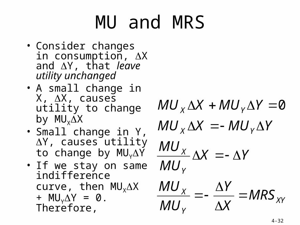
MU and MRS• Consider changes in

consumption, X and Y, that leave utility unchanged

• A small change in X, X, causes utility to change by MUXX

• Small change in Y, Y, causes utility to change by MUYY

• If we stay on same indifference curve, then MUXX + MUYY = 0. Therefore,

4-32

XYY

X

Y

X

YX

YX

MRSX

Y

MU

MU

YXMU

MU

YMUXMU

YMUXMU

0

Utility and Marginal Utility

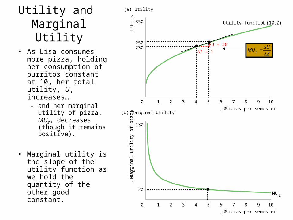
• As Lisa consumes more pizza, holding her consumption of burritos constant at 10, her total utility, U, increases…– and her marginal

utility of pizza, MUZ, decreases (though it remains positive).

• Marginal utility is the slope of the utility function as we hold the quantity of the other good constant. M

UZ,

Mar

gina

l util

ity o

f pi

zza

MUZ

10987654321

Z, Pizzas per semester

0

130

(b) Marginal Utility

20

U,

Util

s

U = 20

Utility function, U (10, Z)

Z = 1

10987654321

Z, Pizzas per semester

0

350

250

(a) Utility

230

Z

UMU Z

Ordinal utility• The indifference map of the utility function U =

XY will look identical to the indifference map of the utility function V = (XY)2 = U2 or of the utility function W = (XY)2 + 12 = U2 + 12

• That is, the way a utility function ranks various goods bundles is unchanged if the utility numbers given to every bundle are transformed in an order-preserving manner

• The utility numbers themselves are unimportant• Only the implied rankings are important

Ordinal utility• As was just claimed, the indifference map of

the utility function U = XY will look identical to the indifference map of the utility function V = (XY)2 = U2 or of the utility function W = (XY)2 + 12 = U2 + 12

• In particular, MRSXY at any goods bundle will be unaffected if the utility numbers given to every bundle are transformed in an order-preserving manner

Figure 4.12: Perfect Substitutes

4-36

Utility function: U = 2E + RMRSRE = ½

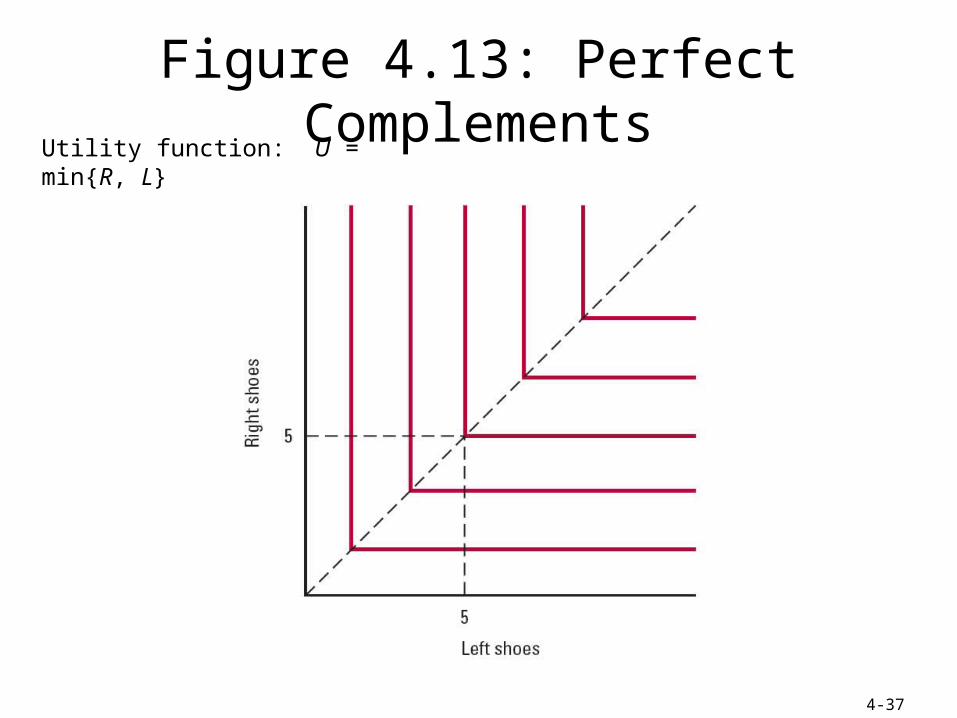
Figure 4.13: Perfect Complements

4-37

Utility function: U = min{R, L}

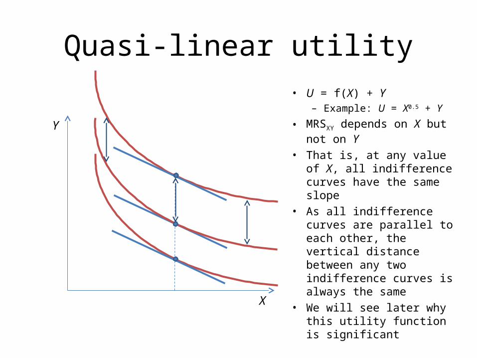
Quasi-linear utility• U = f(X) + Y

– Example: U = X0.5 + Y

• MRSXY depends on X but not on Y

• That is, at any value of X, all indifference curves have the same slope

• As all indifference curves are parallel to each other, the vertical distance between any two indifference curves is always the same

• We will see later why this utility function is significant

X

Y