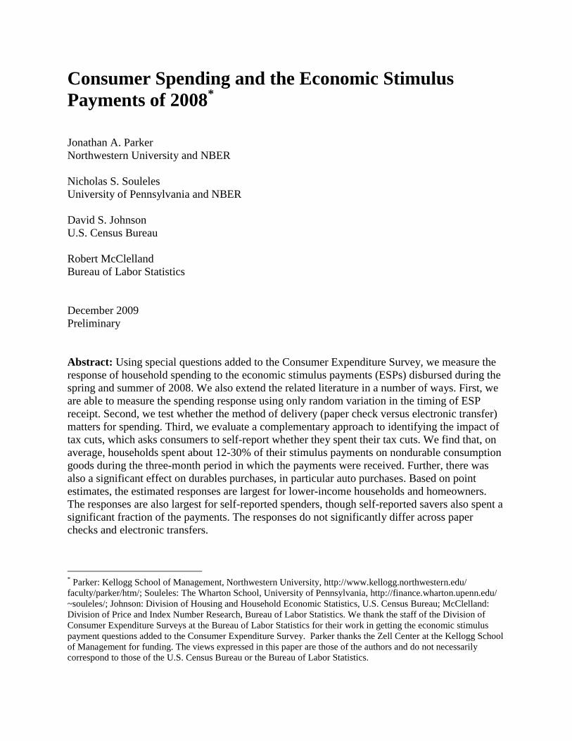
Consumer Spending and the Economic Stimulus Payments of 2008*

Jonathan A. Parker Northwestern University and NBER Nicholas S. Souleles University of Pennsylvania and NBER David S. Johnson U.S. Census Bureau Robert McClelland Bureau of Labor Statistics December 2009 Preliminary Abstract: Using special questions added to the Consumer Expenditure Survey, we measure the response of household spending to the economic stimulus payments (ESPs) disbursed during the spring and summer of 2008. We also extend the related literature in a number of ways. First, we are able to measure the spending response using only random variation in the timing of ESP receipt. Second, we test whether the method of delivery (paper check versus electronic transfer) matters for spending. Third, we evaluate a complementary approach to identifying the impact of tax cuts, which asks consumers to self-report whether they spent their tax cuts. We find that, on average, households spent about 12-30% of their stimulus payments on nondurable consumption goods during the three-month period in which the payments were received. Further, there was also a significant effect on durables purchases, in particular auto purchases. Based on point estimates, the estimated responses are largest for lower-income households and homeowners. The responses are also largest for self-reported spenders, though self-reported savers also spent a significant fraction of the payments. The responses do not significantly differ across paper checks and electronic transfers.

* Parker: Kellogg School of Management, Northwestern University, http://www.kellogg.northwestern.edu/ faculty/parker/htm/; Souleles: The Wharton School, University of Pennsylvania, http://finance.wharton.upenn.edu/ ~souleles/; Johnson: Division of Housing and Household Economic Statistics, U.S. Census Bureau; McClelland: Division of Price and Index Number Research, Bureau of Labor Statistics. We thank the staff of the Division of Consumer Expenditure Surveys at the Bureau of Labor Statistics for their work in getting the economic stimulus payment questions added to the Consumer Expenditure Survey. Parker thanks the Zell Center at the Kellogg School of Management for funding. The views expressed in this paper are those of the authors and do not necessarily correspond to those of the U.S. Census Bureau or the Bureau of Labor Statistics.

1

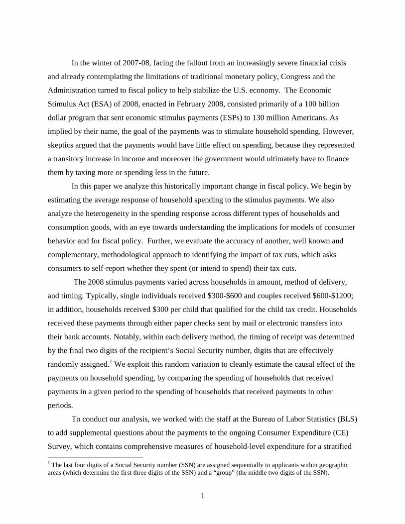
In the winter of 2007-08, facing the fallout from an increasingly severe financial crisis

and already contemplating the limitations of traditional monetary policy, Congress and the

Administration turned to fiscal policy to help stabilize the U.S. economy. The Economic

Stimulus Act (ESA) of 2008, enacted in February 2008, consisted primarily of a 100 billion

dollar program that sent economic stimulus payments (ESPs) to 130 million Americans. As

implied by their name, the goal of the payments was to stimulate household spending. However,

skeptics argued that the payments would have little effect on spending, because they represented

a transitory increase in income and moreover the government would ultimately have to finance

them by taxing more or spending less in the future.

In this paper we analyze this historically important change in fiscal policy. We begin by

estimating the average response of household spending to the stimulus payments. We also

analyze the heterogeneity in the spending response across different types of households and

consumption goods, with an eye towards understanding the implications for models of consumer

behavior and for fiscal policy. Further, we evaluate the accuracy of another, well known and

complementary, methodological approach to identifying the impact of tax cuts, which asks

consumers to self-report whether they spent (or intend to spend) their tax cuts.

The 2008 stimulus payments varied across households in amount, method of delivery,

and timing. Typically, single individuals received $300-$600 and couples received $600-$1200;

in addition, households received $300 per child that qualified for the child tax credit. Households

received these payments through either paper checks sent by mail or electronic transfers into

their bank accounts. Notably, within each delivery method, the timing of receipt was determined

by the final two digits of the recipient’s Social Security number, digits that are effectively

randomly assigned.1 We exploit this random variation to cleanly estimate the causal effect of the

payments on household spending, by comparing the spending of households that received

payments in a given period to the spending of households that received payments in other

periods.

To conduct our analysis, we worked with the staff at the Bureau of Labor Statistics (BLS)

to add supplemental questions about the payments to the ongoing Consumer Expenditure (CE)

Survey, which contains comprehensive measures of household-level expenditure for a stratified 1 The last four digits of a Social Security number (SSN) are assigned sequentially to applicants within geographic areas (which determine the first three digits of the SSN) and a “group” (the middle two digits of the SSN).

2

random sample of U.S. households. Like a similar module of questions about the 2001 tax

rebates analyzed by Johnson, Parker, and Souleles (2006) [JPS], the 2008 questions ask CE

households to report the amount and month of receipt of each stimulus payment they received.

The 2008 survey also includes some new types of questions. It asks about the method of

delivery of each payment (mailed paper check versus electronic transfer). Further, it asks

households who received payments to directly self-report whether they mostly spent or mostly

saved their payments. This question mimics the questions in the Michigan Survey of Consumers

that have been used to study recent changes in tax policy, as in Shapiro and Slemrod (2003a).

One of the advantages of such questions is that they can be put into the field and analyzed

quickly after the announcement of policy changes.

In addition to analyzing the 2008 ESPs, our paper builds on the related literature in a

number of ways. First, relative to JPS, we are able to measure with precision the response of

spending even when using only random variation in the timing of ESP receipt. Second, we

consider whether the delivery method (check versus electronic) affects the amount of spending.

This is an important consideration since the 2008 tax cut was the first large tax cut to use

electronic transfers, and electronic transfers will be used increasingly frequently in the future.

Third, we evaluate the accuracy of the self-reported responses to the payments, by comparing the

results to the results using the data on actual spending and ESP receipt.

Summarizing our main findings, on average households spent about 12-30% of their

stimulus payments, depending on the specification, on nondurable consumption goods during the

three-month period in which the payments were received. This response is statistically and

economically significant. Although our findings do not depend on any particular theoretical

model, the response is inconsistent with both Ricardian equivalence, which implies no spending

response, and with the canonical life-cycle/permanent income hypothesis (LCPIH), which

implies that households should consume at most the annuitized value (on the order of about 5%)

of a transitory increase in income like that induced by the one-time payments. We also find a

significant effect on durables purchases, bringing the average response of total consumption

expenditures to about 50-90% of the payments in the quarter of ESP receipt. In particular, auto

purchases were greater than they would have been in the absence of the payments.

These results are broadly consistent and significant across specifications that use different

forms of variation, including specifications that rely on just the randomized timing variation

3

within each of the two delivery methods. We also find some evidence of an ongoing though

smaller response in the subsequent three-month period after ESP receipt, but this response cannot

be estimated with precision.

Across households, according to the point estimates, the responses are largest for lower-

income households, older households, and homeowners, although these differences are not

statistically significant. The responses are also largest for self-reported spenders, yet self-

reported savers (including those reporting they reduced debt) also spent a statistically and

economically significant fraction of their payments. The responses do not significantly differ

across paper checks and electronic transfers.

This paper is structured as follows. Sections I and II briefly describe the literature and

relevant aspects of ESA 2008. Section III describes the data and Section IV sets forth our

empirical methodology. Section V presents the main results regarding the short-run response to

the economic stimulus payments, while Section VI examines the longer-run response. Section

VII examines the differences in response across different households and consumption goods,

and a final section concludes. The Appendix contains additional information about the data.

I. Related Literature

Many papers have tested the consumption-smoothing implications of the rational-

expectations LCPIH. One related set of papers uses household-level data and quasi-experiments

to identify the effects on consumption from various changes in household income. A smaller set

of papers estimates the consumption effects from changes in tax policy in particular. See Deaton

(1992), Browning and Lusardi (1996), and Johnson, Parker, and Souleles (2006) for reviews.2

Our paper is most closely related to JPS (2006), which uses a similar module of questions

appended to the CE survey to study the 2001 income tax rebates. JPS finds that households spent

about 20-40 percent of their rebates on nondurable goods during the three-month period in which

they received their rebates. There is also a significant though decaying lagged spending effect, so

that roughly two-thirds of the rebates was spent cumulatively during the quarter of receipt and

subsequent three-month period. The responses are largest for households with low liquid wealth

or low income, which is suggestive of binding liquidity constraints. Agarwal, Liu, and Souleles

(2007) finds consistent results using credit card data and direct indicators of being credit

2 For a survey of recent fiscal policy, see e.g., Auerbach and Gale (2009).

4

constrained; in particular, the spending responses are largest for consumers that are constrained

by their credit limits. Johnson, Parker, and Souleles (2009) finds qualitatively similar responses

to the 2003 child tax credit payments, using CE data.3

Our paper is also closely related to studies that evaluate tax policy by asking households

to self-report whether they spent tax cuts. Shapiro and Slemrod (2003a) finds, using the

Michigan Survey of Consumers, that about 22% of respondents who received (or expected to

receive) a 2001 rebate report that they will mostly spend their rebate. The authors calculate that,

under certain assumptions, this result implies an average marginal propensity to consume (MPC)

of about one third, which is consistent with the short-run response of expenditure in JPS

estimated from data on actual spending and rebate receipt. More recently, Shapiro and Slemrod

(2009) uses the Michigan Survey to analyze the 2008 stimulus payments and finds similar

results, with about 20% of respondents reporting that they will mostly spend their payment. This

again corresponds to an average MPC of about one third. This response is larger than expected

under the LCPIH for a transitory tax cut, and it implies a noticeable expansionary effect on

aggregate consumption in the second and third quarters of 2008, the period during which and

shortly after most of the payments were disbursed. The Michigan survey results provide no clear

evidence of greater spending by low-income or potentially constrained households.4

Also studying the 2008 ESPs, using scanner data on a subset of nondurable retail goods

in the first few weeks after the payments started to be sent out, Broda and Parker (2008) finds

that spending on such goods increased by a significant amount, 3.5% in the four weeks after

payment receipt. The increase is larger for low asset and low income households. Using the CE

survey, we will examine broader measures of expenditure over a longer period of time.5

3 Coronado, Lupton, and Sheiner (2006) also study the 2003 child payments, using the Michigan Survey. 4 In 2008, of the 80% of respondents who report they will mostly save their ESP, the majority (about 60%) report that they will mostly pay down debt (as opposed to accumulate assets). See also Sahm, Shapiro and Slemrod (2009). The Michigan Survey includes additional questions to try to determine whether there was a lagged response to the rebate. Of respondents who said they will initially mostly use the rebate to pay down debt, most report that they will “try to keep [down their] lower debt for at least a year.” (There are analogous results for respondents who said they will save by accumulating assets.) The Survey included similar questions in 2001 and yielded similar results (Shapiro and Slemrod, 2003b). By contrast, using data on actual spending in 2001, Agarwal, Liu, and Souleles (2007) finds that, while on average households initially used some of their rebates to increase credit card payments and thereby pay down debt, the resulting liquidity was soon followed by a substantial increase in spending. 5 Using data from a payday lender, Bertrand and Morse (2009) finds that receipt of an ESP reduces the probability of taking out a payday loan for two pay cycles. The effect dissipates by the third cycle, and the magnitude of the reduction in debt is modest relative to the stimulus payments. Such results are qualitatively consistent with the spending dynamics discussed in Agarwal, Liu, and Souleles (2007).

5

As noted above, our paper builds on the previous literature in a number of additional

ways. First, as a result of the new types of questions added to the CE survey in 2008, we can

consider whether the delivery method matters, as well as the accuracy of the self-reported

responses to the payments. Second, although the results in JPS remained consistent (in the

Hausman sense) across specifications that used different forms of variation, they lost statistical

significance when limited to only randomized timing variation. Here we further explore this

issue and obtain greater precision. Third, there are some potentially important differences in the

details of the tax cut (as discussed in the next section) and economic environment in 2008

compared to earlier periods. For instance, on average the stimulus payments in 2008 were about

twice the size of the rebates in 2001. Some prior research suggests the possibility that larger

payments could lead to a different composition of spending. While JPS finds no significant

response of durable goods in 2001, Souleles (1999) finds a significant increase in both

nondurable and durable goods (in particular auto purchases) in response to spring-time Federal

income tax refunds, which are substantially larger than the 2001 tax rebates.6 Also, in 2008

housing and mortgage markets were in turmoil and so we will also examine the response of

homeowners and mortgage borrowers to the ESP.

II. The 2008 Economic Stimulus Payments

ESA 2008 provided ESPs to the majority of U.S. households (roughly 85% of “tax

units”). The ESP consistent of a basic payment, typically $600 or $1200, and -- conditional on

eligibility for the basic payment -- a supplemental payment of $300 per child that qualified for

the child tax credit. To be eligible for the basic payment, a household needed to have positive net

income tax liability, or at least sufficient “qualifying income”.7 For qualifying households, the

basic payment was generally the maximum of $300 ($600 for couples filing jointly) and their tax

liability up to $600 ($1200 for couples). Households without tax liability received basic

6 See also Barrow and McGranahan (2000) and Adams, Einav, and Levin (2009) for related results for the EITC and for subprime auto sales. Federal tax refunds currently average around $2500 per recipient, whereas the average rebate in 2001 came to about $480 (JPS). 7 While the stimulus payments were commonly referred to as “tax rebates,” strictly speaking they were advance payments for credit against tax year 2008 taxes. To expedite the disbursement of the payments, they were calculated using data from the tax year 2007 returns (and so only those filing 2007 returns received the payments). If subsequently a household’s tax year 2008 data implied a larger payment, the household could claim the difference on its 2008 return filed in 2009. However, if the 2008 data implied a smaller payment, the household did not have to return the difference.

6

payments of $300 ($600 for couples), so long as they had at least $3000 of qualifying income

(which includes earned income and Social Security benefits, as well as certain Railroad

Retirement and veterans’ benefits). Eligibility started to phase out at a threshold of $75,000 of

adjusted gross income (AGI) ($150,000 for couples), with the basic payment being reduced by

five percent of the amount by which AGI exceeded the threshold. (Thus the payments

completely phased out at $87,000 for individuals and $174,000 for couples). Because of this

phase-out for higher income households, and the payments to households without tax liability,

the stimulus payments were generally more targeted to lower income households than were the

2001 income tax rebates.

In terms of timing, for recipients who had provided the IRS with their bank routing

number (i.e., for direct deposit of tax refunds8), the stimulus payments were disbursed

electronically over a three-week period ranging from late April to mid May. Otherwise, the

payments were mailed (using paper checks) over a nine-week period ranging from mid May to

mid July.9 In both cases, the particular timing of the payments was determined by the last two

digits of the recipients’ Social Security numbers, which are effectively randomly assigned.

In aggregate, the stimulus payments in 2008 were historically large, amounting to about

$100 billion, which is more than double the size of the 2001 rebate program. According to the

Treasury, $78.8 billion in ESPs were disbursed in the second quarter of 2008, which corresponds

to about 2.2% of GDP or 3.1% of personal consumption expenditures in that quarter. During the

third quarter, $15 billion in ESPs were disbursed, corresponding to about 0.4% of GDP or 0.6%

of personal consumption expenditures. The stimulus payments constituted about two-thirds of

the total ESA package, which also included various business incentives and foreclosure relief.10

This paper focuses on the stimulus payments, as recorded in our CE dataset.11

8 Payments were directly deposited only to personal bank accounts. Payments were mailed to tax filers who had provided the IRS with their tax preparer’s routing number as part of taking out a “refund anticipation loan”. The latter are common, representing about a third of the tax refunds delivered via direct deposit in 2007. 9 Due to the electronic deposits, about half of the aggregate stimulus payments were disbursed by the end of May. While most of the rest of the payments came in June and July, taxpayers that filed their 2007 return late could receive their payment later than the above schedule. Since 92 percent of taxpayers typically file at or before the normal April 15th deadline (Slemrod et al., 1997), this source of variation is small. Nonetheless, we present results below that exclude such late rebates. 10 For more details on ESA, see e.g., CCH (2008) and Shapiro and Slemrod (2009). 11 Our empirical approach focuses on consumers’ response to the receipt of their stimulus payments, a point in time that our data identifies. Our methodology cannot estimate the magnitude of any earlier response that may have occurred in anticipation of the payments, both because the passage of ESA cannot be separated from other aggregate

7

III. The Consumer Expenditure Survey

The CE interview survey contains detailed measures of the expenditures of a stratified

random sample of U.S. households. CE households are interviewed up to four times, three

months apart, to collect expenditure information. In each interview households report their

expenditures during the preceding three months (the “reference period”). New households are

added to the survey every month so that the data are effectively monthly in frequency. In

addition to surveying households about their expenditures, the CE also gathers (less-frequent)

information about their demographic characteristics, income, and wealth. We use the 2007 and

2008 waves of the CE data (which include interviews in the first quarter of 2009).

The extra questions about the 2008 ESPs were included in the CE Survey in interviews

conducted in June 2008 to March 2009, which cover the crucial time during which the payments

were disbursed. The first set of questions asked households whether they received any

“economic stimulus payments… also called a tax rebate” since the beginning of the reference

period for the interview. If so, the questions asked for the amount of each payment and the date it

was received, and whether it was received by check or direct deposit. These questions were

phrased to be consistent with the style of other CE questions, and were asked in all interviews

that households had during the period in which the ESP questions were in the field.

Households reporting a payment were subsequently asked whether they think the

payment led them “mostly to increase spending, mostly to increase savings, or mostly to pay off

debt.” This question was asked just once of each household. The wording of the question closely

follows the main question in the Michigan Survey of Consumers analyzed by Shapiro and

Slemrod (2009).

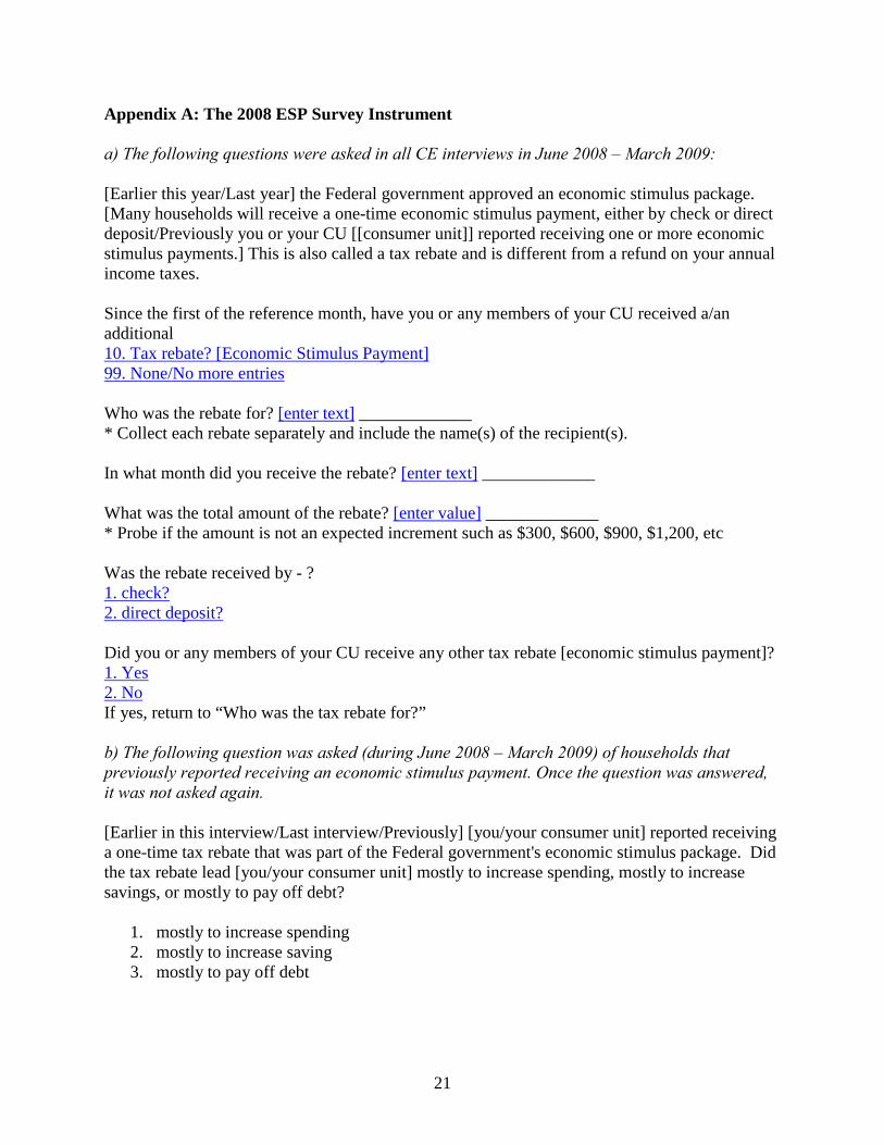
Appendix A contains the language of the survey instrument. We follow JPS in

constructing the total payments received by each household in each three-month expenditure

reference-period.

We also follow JPS in our definition of expenditures. Specifically, we focus on a series of

increasingly aggregated measures of consumption expenditures. First, we study expenditures on

food, which include food consumed away from home, food consumed at home, and purchases of

effects captured by our time dummies, such as seasonality, and because there is no single point in time at which a tax cut went from being entirely unexpected to being entirely expected.

8

alcoholic beverages. Much previous research has studied such expenditure on food, largely

because of its availability in the Panel Study of Income Dynamics, but it is a narrow measure of

expenditure. Our second and main measure of consumption expenditures is nondurable

expenditures, which is a broad measure of expenditures on nondurable goods and services,

following previous research. Third, we also consider a subset of nondurable expenditures,

“strictly nondurable” expenditures, which excludes semi-durable goods like apparel, following

Lusardi (1996). Finally, total expenditures includes both nondurable expenditures and durable

expenditures, such as auto purchases.12 Appendix B provides further details about the data.

Our sample includes only households that had at least one interview during the period in

which the ESP questions were in the field. The resulting sample period starts with interviews in

December 2007 (when period t+1 in equation (1) below covers expenditures in September 2007

to November 2007) and runs through interviews in March 2009 (when period t+1 covers

December 2008 to February 2009). Also, we drop from the sample any household observation (t

or t+1) with implausibly low expenditures (the bottom 1% of nondurable expenditures in levels),

unusually large changes in age or family size, and uncertain stimulus payment status.

Table 1 presents summary statistics for our dataset. For each household-reference quarter,

we sum all stimulus payments received by the household in that quarter to create our main

economic stimulus payment variable, ESP. During the consumption reference period that covers

the main time of disbursement of the payments (May - July), about two-thirds of households

report receiving a payment. The average value of ESP, conditional on a positive value, is about

$1000.

IV. Empirical Methodology

Consistent with specifications in the previous literature (e.g., Zeldes (1989a), Lusardi

(1996), Parker (1999), Souleles (1999), and JPS), our main estimating equation is:

Ci,t+1 - Ci,t = s 0s*months,i + 1'Xi,t + 2 ESPi,t+1 + ui,t+1 , (1)

where C is either consumption expenditures or their log; month is a complete set of indicator

variables for every period in the sample, used to absorb the seasonal variation in consumption

expenditures as well as all other concurrent aggregate factors; and X are control variables (here

12 Unlike in JPS, the response of total expenditures is estimated below with relative precision. This could in part reflect the larger total number of payments (about 30% more) in the sample in 2008, and the larger size (over double) of these payments.

9

age and changes in family size) included to absorb some of the preference-driven differences in

the growth rate of consumption expenditures across households. ESPi,t+1 represents our key

stimulus payment variables, which take one of three forms: i) the total dollar amount of stimulus

payments received by household i in period t+1 (ESPi,t+1); ii) a dummy variable indicating

whether any payment was received in t+1 (I(ESPi,t+1>0)); and iii) a distributed lag of ESP or

I(ESP >0), to measure the longer-run effects of the payments. We correct the standard errors to

allow for arbitrary heteroskedasticity and within-household serial correlation. As an extension, to

analyze heterogeneity in the response to the payments, we interact ESPi,t+1 with indicators for

different types of households.

The key coefficient 2 measures the average response of household expenditure to the

stimulus payments. Using the randomized timing of ESP receipt helps us avoid any potential

omitted variables bias, and so provides a clean estimate of the causal effect of the payments. For

nondurable expenditures, this estimate provides a direct test of the LCPIH. Since Congress

passed ESA in February, 2008, and expectations of some tax cut arose even earlier, the payment

can be thought of as being pre-announced.13 In this case, the rational-expectations LCPIH

implies that 2=0. Even if instead households were actually surprised by the payment, 2 should

still be small under the LCPIH, because the one-time payment represents a transitory increase in

income. 2 should also be zero under Ricardian equivalence.

V. The Short-Run Response of Expenditure

This section estimates the short-run change in consumption expenditures caused by

receipt of the stimulus payments, using the contemporaneous payment variables ESPt+1 and

I(ESPt+1>0) in equation (1). The following section estimates the lagged response to the

payments.

In light of potential measurement error and sample-size limitations, in working with

household-level data on expenditure it is in general important to use the largest possible sample

13 Since February 2008 can fall in period t for some sample households receiving a payment, any announcement effect from the passage of ESA could potentially attenuate our estimate of 2. However, whenever information about the tax cuts underlying the ESPs became publicly available, whether preceding the actual passage of ESA or not, any resulting wealth effects should be small, and should have arisen at the same time(s) for all consumers, so their average effects on expenditure would be picked up by the corresponding time dummies in equation (1). Even heterogeneity in such wealth effects would not be correlated with the timing of ESP receipt, so 2 should still equal zero when estimated using randomized timing variation.

10

and as much variation as possible in the relevant independent variables. Accordingly we begin

by estimating equation (1) utilizing all of the available information about the payments received

by each household, using ESP as the key regressor. While this variable is analogous to that used

in most tests of the LCPIH, we can go further and investigate its validity by limiting the amount

of variation that we utilize, e.g. by using I(ESP >0), which includes only variation in whether a

payment was received at all in a given period, not the dollar amount of payments received.

In Table 2, the first set of four columns displays the results of estimating equation (1) by

ordinary least squares (OLS), with the dollar change in consumption expenditures as the

dependent variable and the contemporaneous amount of the payment (ESPt+1) as the key

independent variable, which uses all available payment information. The resulting estimates of

2 measure the average fraction of the payment spent on the different expenditure aggregates in

each column, within the three-month reference-period in which the payment was received. We

find that, during the three-month period in which a payment was received, relative to the

previous three-month period, a household on average increased its expenditures on food by about

2 percent of the payment, its expenditures on strictly nondurable goods by 8 percent of the

payment, and its expenditures on nondurable goods by 12 percent of the payment. The third

result is statistically significant, and larger than implied by the LCPIH. In the fourth column,

total consumption expenditures increased on average by 52 percent of the payment, a substantial

and statistically significant amount. This result is relatively precisely estimated, especially

considering that the difference with the preceding results reflects durables expenditures, which

are much more volatile than nondurable expenditures.

These results identify the effect of a payment from variation in both the timing of

payment receipt and the dollar amount of the payment. While the variation in the payment

amount is possibly uncorrelated with the residual in equation (1), it is not purely random since

the amount depends upon household characteristics such as tax status, income, and number of

dependents.

The remaining columns of Table 2 use only variation in whether a payment was received

at all in a given period, not the dollar amount of payments received. The second set of columns

in the table uses the indicator variable I(ESPt+1>0) in equation (1). In this case 2 measures the

average dollar increase in expenditures caused by receipt of a payment. The estimated responses

again increase in magnitude across the successive expenditure aggregates. During the three-

11

month period in which a payment was received, relative to the previous three-month period,

households on average increased their expenditures on nondurable goods by $122, which is

statistically significant at the 7% level. Total expenditures increased by a significant $494.

Compared to an average payment of about $1000, these results are consistent with the previous

estimates in the first set of columns, which also used variation in the magnitude of the payments

received.

As a robustness check, the third set of columns in Table 2 uses the change in log

expenditures as the dependent variable. On average in the three-month period in which a

payment was received, relative to the previous three-month period, nondurable expenditure

increased by 2.1%, and total expenditures increased by 3.2%. These are again statistically and

economically significant effects. Considering the magnitudes of nondurable and total

expenditures (Table 1), these results are broadly consistent with the previous results in the table.

Finally, since it is interesting to estimate a value interpretable as a marginal propensity to

spend upon the payment’s arrival, we estimate equation (1) by two-stage least squares (2SLS).

We instrument for the payment amount, ESP, using the indicator variable, I(ESP >0), along with

the other independent variables. As in the first four columns, 2 then measures the fraction of the

payment that is spent within the three-month period of receipt – but in this case without using

variation in the magnitude of the payment. As shown in the last set of columns in Table 2, the

estimated marginal propensities to spend remain close in magnitude to those estimated in the first

four columns, which did not treat ESP as potentially non-exogenous.14

The results in Table 2 identify the effect on spending by comparing the behavior of

households that received payments at different times to the behavior of households that did not

receive payments at those times. Since some households did not receive any payment, in any

period, the results still use some information that comes from comparing households that

received payments to those that never received payments. Table 3 investigates the role of this

variation using a number of different approaches, for brevity focusing on strictly nondurable

goods, nondurable goods, and total expenditures. 14 The findings in Table 2 are generally robust across a number of additional sensitivity checks. For instance, using median regressions or winsorizing the dependent variable lead to very similar results for food, strictly nondurable goods, and nondurable goods. For total expenditures, the resulting coefficients are generally smaller than in Table 2, though still statistically and economically significant (e.g., substantially larger than those for nondurable expenditures). This reduction in point estimates for total expenditures is to be expected, since the distribution of expenditure changes (dC) has much more of its mass in the tails for total expenditures than for nondurable expenditures. Weighting the sample leads to very similar results as in Table 2, for all four expenditure aggregates.

12

First, Panel A adds to equation (1) an indicator for households that received a payment in

any reference quarter, I(Total ESP >0), which allows the expenditure growth of payment

recipients to differ on average from that of non-recipients. In this case, the main regressor

I(ESPt+1>0) captures only high-frequency variation in the timing of payment receipt -- receipt in

quarter t+1 in particular -- conditional on receipt in some quarter. As reported in Table 3, the

estimated coefficients on I(Total ESP >0) are always small and statistically insignificant. Hence,

apart from the effect of the payment, the expenditure growth of payment recipients is on average

similar to that of non-recipients over the quarters in the sample period around the payments.

Moreover, the estimated coefficients for the effect of the payment (ESPt +1 and I(ESPt +1>0)) are

rather similar to those in Table 2. Hence the results in Table 2 are not driven by differences in

expenditure growth between payment recipients and non-recipients over the sample period. That

is, controlling for whether a household ever received a payment, spending significantly increases

in the particular quarter of payment receipt.

Our second approach is more stringent. Panel B excludes from the sample all households

that did not receive a payment in some reference quarter. (Conservatively, it excludes all the

households not known to have received a payment based on the available data.) The advantage of

this approach is that, when using I(ESP>0), it identifies the response of spending using only the

variation in the timing of payment receipt conditional on receipt, by comparing the spending of

households that received payments in a given period to the spending of households that also

received payments but in other periods. The disadvantage of the approach is that it leads to a

reduction in power due to the resulting decline in sample size and effective variation.

Nonetheless, the results are broadly consistent with the previous results (especially when

considering the confidence intervals). While as expected the standard errors increase, the point

estimates are also somewhat larger than before, and so the results are all statistically significant.

Finally, Panel C also excludes the households that received late stimulus payments, after

the main period of their (randomized) disbursement, due to filing late tax returns in the preceding

year. Although the timing of these payments is not necessarily endogenous, it was not

randomized.15 In JPS, analogously limiting the sample to non-late rebate recipients significantly

reduced the precision of the results. Here by contrast the results remain statistically significant.

15 Extending JPS to accommodate the two delivery methods, we exclude paper checks received after August, and electronic ESPs received after June.

13

They also remain economically significant, broadly consistent in magnitude with the preceding

results. In the final set of columns using 2SLS, on average nondurable expenditures increased by

31% of the payment in the quarter of receipt, relative to the previous quarter, and total

expenditures increased by 91% of the payment. In sum, even when limiting the variation to the

timing of ESP receipt conditional on (non-late) receipt, the results imply that the ESPs had a

significant effect on household spending.

Table 4 examines one of the key new features of the ESP program, the use of electronic

funds transfers (EFT). About 40% of the CE households received their payments via EFTs, and

the use of EFTs is likely to increase in the future, so it is important to consider whether the

method of payment delivery matters. Panel A separately estimates the average response of

spending to EFTs and to paper checks, using their analogues of ESP and I(ESP>0), starting with

the entire sample of households from Table 2.16 The estimated coefficients are generally similar

(and not statistically significantly different) across the two delivery methods, across all the

columns. Thus these results provide no evidence that the method of delivery affected the average

response of spending.

The rest of Table 4 returns to the investigation of different forms of variation, following

Table 3, now taking into account that the method of delivery (paper check versus EFT) was not

randomized. For example, households receiving EFTs have somewhat higher income on average

than households receiving paper checks, and might also be different in other, hard to observe

ways (e.g., perhaps they are more technologically savvy). Panel B again restricts the sample to

households receiving non-late stimulus payments, as in the final panel of Table 3. Not

surprisingly, since the EFTs were disbursed over just a few weeks, using just timing variation

leads to a significant reduction in power for estimating the effect of EFT receipt. More

importantly, the results for paper checks remain statistically significant and broadly similar to the

average response in the final panel of Table 3. That is, even separately controlling for receipt of

EFTs, using the random variation in the timing of the paper checks still yields a significant

response of spending to the paper checks.

Strictly speaking, these results still impose common month dummies and demographic

effects (age and changes in family size) across EFT and paper-check recipients. One could relax

this imposition by estimating equation (1) for separate samples of EFT and paper-check

16 A few observations have missing values for the method-of-delivery question, and so are dropped from the sample.

14

recipients, however some households, albeit a small fraction (about 2%), received both EFTs and

paper checks. Also, our goal here is to estimate the average response to the stimulus payments,

using clearly exogenous variation. Accordingly, Panel C of Table 4 estimates a pooled regression

that allows for separate time dummies and demographic effects across three groups of

households: a) households who received only paper checks; b) households who received only

EFTs; c) households who received both paper checks and EFTs. The results are broadly similar

to those in the final panel of Table 3, even though they are driven by the random variation in the

timing of just paper checks (since the EFTs have limited timing variation).17

Overall, our findings remain broadly consistent across specifications that use different

forms of variation, including very limited variation. Not surprisingly, at times the point estimates

vary somewhat across specifications, especially for total expenditures, but not significantly so

relative to the corresponding confidence intervals, and the conclusions regarding statistical and

economic significance remain robust. In particular, even when limiting our variation to only

randomized variation in the timing of ESP receipt, we find that the payments caused a significant

increase in household spending in the short-run.

VI. The Longer-Run Response of Expenditure

To investigate the longer-run effect of the stimulus payments, we add the first lag of the

payment variable, ESPt, as an additional regressor in equation (1), focusing on the households

that received non-late payments as in the final panel of Table 3. The resulting estimates are

reported in Table 5.

First, note that the presence of the lagged variable does not alter our previous conclusions

about the short-run impact of the payment. The coefficients on ESPt+1 are broadly similar to the

corresponding results in Table 3. Second, the receipt of a payment causes a change in spending

one quarter later (i.e., from the three-month period of receipt to the next three-month period) that

is negative but smaller in absolute magnitude than the contemporaneous change. Since the net

effect of the payment on the level of spending in the later quarter (relative to the level in the

quarter before receipt) is given by the sum of the coefficients on ESPt and ESPt+1, this implies

17 Across all the columns in Panel C, the coefficients on the time dummies (jointly) and the demographic variables (jointly) never significantly vary across the two main groups of households, those who received only EFTs and those who received only paper checks. These coefficients are sometimes significant only for the few households who received both EFTs and paper checks, relative to the two main groups.

15

that, after increasing in the three-month period of payment receipt, spending remains high, but

less high, in the subsequent three-month period.

These lagged effects are, however, estimated with less precision. For example, in the

second-to-last column, for nondurable expenditures using 2SLS, nondurable expenditures rise by

25% of the payment in the quarter of receipt. The expenditure change in the next quarter is -10%,

so that nondurable expenditures in the second three-month period are still higher on net than

before payment receipt by 25%-10% = 15% of the payment. The cumulative change in

nondurable expenditures over both three-month periods is then estimated to be 25% + 15% ≈

41% of the payment (bottom row). However, neither the 15% change in the second period nor

the 41% cumulative change is statistically significant. The second-period and cumulative

changes are also insignificant for the other expenditure groups (strictly nondurable goods and

total expenditures) using 2SLS in the final set of columns.

In sum, while the point estimates suggest some ongoing though decaying spending

response to the ESPs in the subsequent quarter after receipt, this lagged response cannot be

estimated with precision, even on average over the sample period. Hence, in the subsequent

extensions where we will push the data harder to consider various forms of heterogeneity, we

will focus on the short-run response.

VII. Differences in Responses across Households and Goods

This section analyzes heterogeneity in the response to the stimulus payment, across

different types of households and different subcategories of consumption goods. This analysis

can potentially provide evidence about why household expenditure responded to the payment.

For brevity, we report results from the 2SLS specification, instrumenting the payment ESP (and

any interaction terms) with the corresponding indicator variables for payment receipt I(ESP>0)

(and their interactions, along with the other independent variables), for the sample of households

receiving non-late payments.

The presence of liquidity constraints is a leading explanation for why household spending

might increase in response to a previously expected increase in income. To investigate this

explanation, we test whether households that were relatively likely to be constrained were more

likely to increase their spending upon arrival of a payment. Constrained households may be

unable or unwilling to increase their spending prior to the payment arrival. On the other hand,

16

unconstrained households (e.g., high wealth or high income households) may find the costs of

not smoothing consumption across the arrival of the payment to be small (Caballero, 1995;

Parker, 1999; Sims, 2003; and Reiss, 2004).

Expanding equation (1), we interact the intercept and ESPt+1 variables with indicator

variables (Low and High) based on various household characteristics (all from households’ first

CE interview to minimize any endogeneity). We use three different variables to identify

households that are potentially liquidity constrained: age, income (family income before taxes),

and liquid assets (the sum of balances in checking and saving accounts). While liquid assets is

arguably the most directly relevant of these variables for identifying liquidity constraints, it is the

least well measured and the most often missing in the CE data, so we start with the other two

variables.18 For each variable, we split households into three groups (Low, High, and the

intermediate baseline group), with the cutoffs between groups chosen to include about a third of

the payment recipients in each group.

Table 6 begins by testing whether the propensity to spend the stimulus payment differs by

age. Because young households typically have low liquid wealth and high income growth, they

are disproportionately likely to be liquidity constrained (e.g., Jappelli, 1990; Jappelli et. al.,

1998).19 In the first set of columns in the table, Low refers to young households (40 years old or

younger) and High refers to older households (older than 58), and the coefficients on the

interaction terms with these variables represent differences relative to the households in the

baseline, middle-age group. The point estimates for the interaction terms suggest that, relative to

the baseline middle-aged household, young households spent less of the payment and old

households spent more of the payment. However, these differences are not statistically

significant.

The second set of columns in Table 6 tests for differences in spending across income

groups. The point estimates suggest that low-income households spent a much larger fraction of

their payment than the typical (baseline middle-income) household, especially in total

expenditures. The bottom panel reports the implied total spending for the interacted groups, in

absolute terms. (The uninteracted ESP coefficient in the first row represents the spending for the

18 The CE survey does not include the direct measures of borrowing and credit constraints used by Jappelli (1990) and Jappelli et. al. (1998), or Agarwal, Liu, and Souleles (2007). 19 There is also evidence that some older households increase their spending on receiving their (predictable) pension checks (Wilcox, 1989; and Stephens, 2003). Outside the null LCPIH hypothesis of β2=0, older households might also spend relatively more because they have shorter time horizons.

17

baseline group.) For total spending on total expenditures, of the three groups, only the result for

the low-income households is statistically significant. It is also economically significant,

averaging about 120% of the payment.20 However, while suggestive of possible role for liquidity

constraints, the difference between this result and that for the baseline group, although large at

about 70 percentage points, is not statistically significant.

The last set of columns in Table 6 tests for differences by liquid asset holdings. While the

point estimates suggest less spending by low-asset households, none of the differences are

statistically significant. Indeed, even the total amounts of spending in absolute terms are

insignificant for all three groups, for both nondurable expenditures and total expenditures. The

loss of precision when using the asset variable might reflect the smaller sample sizes due to

missing asset values and measurement error in the available asset values.

One possible complication in assessing liquidity constraints during the sample period is

that households might have expected the recent recession to last longer than usual. If constrained

households expect their constraints to bind for a longer period of time, that would reduce the

magnitude of their response to a payment per period.

Another key characteristic of the recent recession was the large decline in housing wealth

and the reduced ability to borrow against home equity. To examine the potential implications for

the response to the ESPs, the first set of columns in Table 7 splits the sample according to

housing status. The baseline group is renters (23% of the sample), and the two interacted groups

are homeowners with a mortgage (50%) and homeowners without a mortgage (27%). The point

estimates suggest much larger spending responses by both groups of homeowners relative to

renters, though the differences are not statistically significant. In absolute terms, homeowners

have large and significant responses in both nondurable expenditures and total expenditures,

whereas the response of the renters is much smaller and insignificant.21

20 As discussed below, it is not inconsistent for the average spending response to be larger in magnitude than the average payment, even putting aside the confidence intervals for the former, if enough households buy large durables like autos in response to receiving a rebate. 21 The results for homeowners do not simply reflect the preceding results for older households. E.g., if one drops from the sample the households older than 65, the coefficients for nondurable expenditure remain very similar to those reported in the table, for all three groups of households. The coefficients for total expenditure remain very similar for renters and homeowners with mortgages. While the coefficient for total expenditure looses significance for homeowners without mortgages, presumably in part due to the reduced sample of such homeowners, it remains large in magnitude; and as in the table, the coefficient for nondurable expenditure remains significant and is largest for homeowners without mortgages, compared to the other two groups.

18

Finally, we evaluate the alternative methodological approach that identifies the impact of

tax cuts by asking consumers to self-report whether they spent their tax cut. Of the CE

households that received a stimulus payment, 32% reported that they mostly spent their payment,

18% reported they mostly saved it, and 50% reported they used it to pay down debt. In final set

of columns in Table 7, the self-reported spenders did in fact spend more of the payment than the

other groups. In absolute terms their spending is statistically and economically significant. They

spent about 35 percentage points more on nondurable goods than the baseline group, the self-

reported savers, and this difference is statistically significant. The corresponding difference for

total expenditures is even larger in magnitude, but not statistically significant. On the other hand,

even the self-reported “non-spenders” spent significant, albeit smaller, fractions of the payment

in absolute terms. For self-reported savers, the response of total expenditures is statistically

significant and large at 95% of the payment on average. For households who reported they paid

down debt, the response of total expenditures is still large at about 63 percentage points, albeit

insignificant, and the response of nondurable goods is statistically significant and still rather

large at 27% of the payment. In this sense self-reported spending may provide a lower bound on

the actual amount of spending (consistent with Agarwal, Liu, and Souleles, 2007)).

Turning to differences across goods, each column in Table 8 reports the estimated change

in spending for each subcategory of goods within the broad measure of nondurable expenditures

(a complete decomposition). The columns also report, at the bottom of the table, the share of the

overall increase in nondurable expenditures that is accounted for by each of the subcategories.

For benchmarking, one can compare these results to the average share of each subcategory in

nondurable expenditures (last row). Of course, comparisons of different subsets of nondurable

expenditure must be interpreted cautiously because of potential non-separabilities across goods.

Further, note that in general the results are statistically weak, with only the coefficient for

utilities and household operations being statistically significant. This response is roughly in

proportion to the share of this subcategory in nondurable goods. The point estimates also suggest

a disproportionately large response in personal care (and miscellaneous items), tobacco, and

apparel, though these responses are nonetheless statistically insignificant. For such narrow

subcategories of goods there is much more variability in the dependent variable that is unrelated

to the payment regressor. Our previous results, by summing the subcategories into broader

aggregates of nondurable goods, averaged out much of this unrelated variability (such as, for

19

example, whether a trip to the supermarket happened to fall just inside or outside the expenditure

reference-period).

Table 9 provides the analogous decomposition of the response of the durable goods part

of total expenditures. While there are sizable responses on average in housing (which includes

shelter and furniture/appliances) and entertainment (which includes TVs and other electronic

equipment), these responses are statistically insignificant and small relative to their share in

durable goods. The bulk of the response in durables comes in transportation, spending on which

increases by 53% of the payments on average, a statistically and economically significant

amount. Further analysis shows that this result is driven by vehicle purchases. Receipt of a

stimulus payment increased the probability of purchasing a vehicle, relative to the counterfactual

of no payment, and such purchases are large enough in magnitude that they imply large average

responses to the payments.

VIII. Conclusion

We find that on average households spent about 12-30% of their stimulus payments,

depending on the specification, on nondurable consumption goods during the three-month period

in which the payments were received. This response is statistically and economically significant.

It is generally smaller in magnitude (though not significantly different) than the response in

nondurable goods from the 2001 tax rebate, which could reflect the more transitory nature of the

2008 tax cut. Nonetheless, the response in 2008 is larger than implied by the LCPIH or Ricardian

equivalence. Moreover, the composition of spending is different than in 2001, perhaps reflecting

the larger size of the payments in 2008. We find a significant effect on durables purchases,

bringing the average response of total consumption expenditures to about 50-90% of the

payments in the quarter of ESP receipt. In particular, the results imply that auto purchases,

although weakening during the recession, would have been even weaker in the absence of the

payments.

These results are broadly consistent and significant across specifications that use different

forms of variation, including specifications that rely on just the randomized timing variation

within each of the two delivery methods. We also find some evidence of an ongoing though

smaller response in the subsequent three-month period after ESP receipt, but this response cannot

be estimated with precision.

20

Across households, according to the point estimates, the responses are largest for lower-

income households, older households, and homeowners, although these differences are not

statistically significant. The responses are also largest for self-reported spenders, yet self-

reported savers (including those reporting they reduced debt) also spent a statistically and

economically significant fraction of their payments. The responses do not significantly differ

across paper checks and electronic transfers.

21

Appendix A: The 2008 ESP Survey Instrument

a) The following questions were asked in all CE interviews in June 2008 – March 2009: [Earlier this year/Last year] the Federal government approved an economic stimulus package. [Many households will receive a one-time economic stimulus payment, either by check or direct deposit/Previously you or your CU [[consumer unit]] reported receiving one or more economic stimulus payments.] This is also called a tax rebate and is different from a refund on your annual income taxes. Since the first of the reference month, have you or any members of your CU received a/an additional 10. Tax rebate? [Economic Stimulus Payment] 99. None/No more entries Who was the rebate for? [enter text] _____________ * Collect each rebate separately and include the name(s) of the recipient(s). In what month did you receive the rebate? [enter text] _____________ What was the total amount of the rebate? [enter value] _____________ * Probe if the amount is not an expected increment such as $300, $600, $900, $1,200, etc Was the rebate received by - ? 1. check? 2. direct deposit? Did you or any members of your CU receive any other tax rebate [economic stimulus payment]? 1. Yes 2. No If yes, return to “Who was the tax rebate for?” b) The following question was asked (during June 2008 – March 2009) of households that previously reported receiving an economic stimulus payment. Once the question was answered, it was not asked again. [Earlier in this interview/Last interview/Previously] [you/your consumer unit] reported receiving a one-time tax rebate that was part of the Federal government's economic stimulus package. Did the tax rebate lead [you/your consumer unit] mostly to increase spending, mostly to increase savings, or mostly to pay off debt?

1. mostly to increase spending 2. mostly to increase saving 3. mostly to pay off debt

22

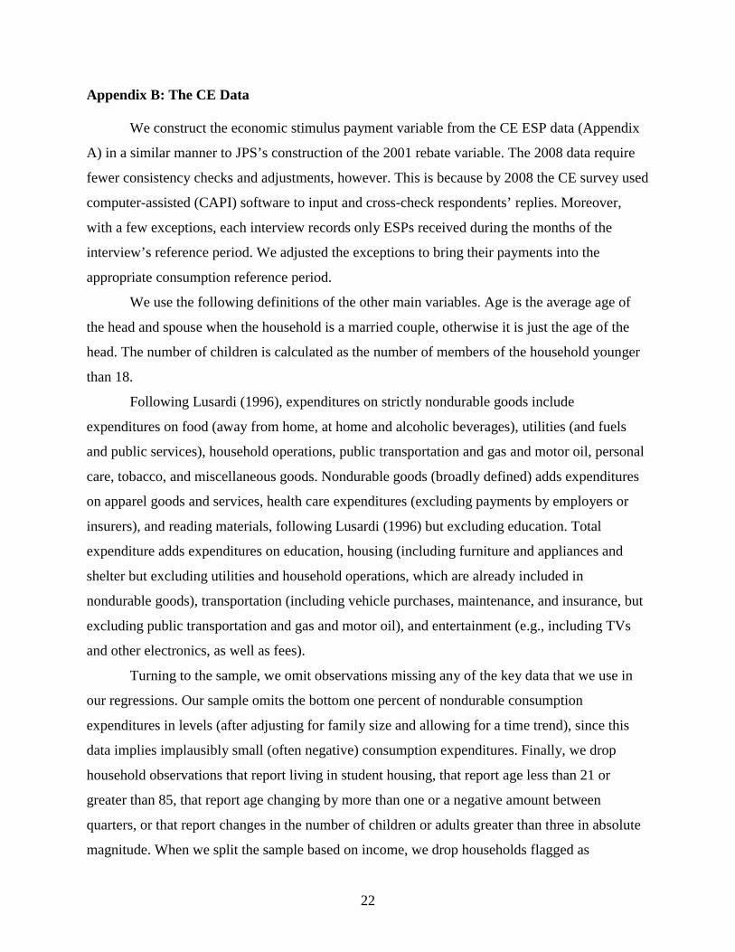
Appendix B: The CE Data

We construct the economic stimulus payment variable from the CE ESP data (Appendix

A) in a similar manner to JPS’s construction of the 2001 rebate variable. The 2008 data require

fewer consistency checks and adjustments, however. This is because by 2008 the CE survey used

computer-assisted (CAPI) software to input and cross-check respondents’ replies. Moreover,

with a few exceptions, each interview records only ESPs received during the months of the

interview’s reference period. We adjusted the exceptions to bring their payments into the

appropriate consumption reference period.

We use the following definitions of the other main variables. Age is the average age of

the head and spouse when the household is a married couple, otherwise it is just the age of the

head. The number of children is calculated as the number of members of the household younger

than 18.

Following Lusardi (1996), expenditures on strictly nondurable goods include

expenditures on food (away from home, at home and alcoholic beverages), utilities (and fuels

and public services), household operations, public transportation and gas and motor oil, personal

care, tobacco, and miscellaneous goods. Nondurable goods (broadly defined) adds expenditures

on apparel goods and services, health care expenditures (excluding payments by employers or

insurers), and reading materials, following Lusardi (1996) but excluding education. Total

expenditure adds expenditures on education, housing (including furniture and appliances and

shelter but excluding utilities and household operations, which are already included in

nondurable goods), transportation (including vehicle purchases, maintenance, and insurance, but

excluding public transportation and gas and motor oil), and entertainment (e.g., including TVs

and other electronics, as well as fees).

Turning to the sample, we omit observations missing any of the key data that we use in

our regressions. Our sample omits the bottom one percent of nondurable consumption

expenditures in levels (after adjusting for family size and allowing for a time trend), since this

data implies implausibly small (often negative) consumption expenditures. Finally, we drop

household observations that report living in student housing, that report age less than 21 or

greater than 85, that report age changing by more than one or a negative amount between

quarters, or that report changes in the number of children or adults greater than three in absolute

magnitude. When we split the sample based on income, we drop households flagged as

23

incompletely reporting income. When we split based on liquid assets, we drop households if the

asset information used in computing initial assets (as the difference between final assets and the

change in assets) is topcoded.

24

References

Adams, William, Einav, Liran, and Levin, Jonathan, “Liquidity Constraints and Imperfect

Information in Subprime Lending,” American Economic Review, 99(1), March, pp. 49-84.

Agarwal, Sumit; Liu, Chunlin and Souleles, Nicholas S., 2007, “The Response of Consumer

Spending and Debt to Tax Rebates – Evidence from Consumer Credit Data,” Journal of

Political Economy, 115(6), December, pp. 986-1019.

Auerbach, Alan J., and Gale, William G., 2009, “Activist Fiscal Policy to Stabilize Economic

Activity,” working paper, September.

Barrow, Lisa, and McGranahan, Leslie, 2000, “The Effects of Earned Income Credit on the

Seasonality of Household Expenditures,” National Tax Journal, December, 53, pp. 1211-44.

Bertrand, Marianne, and Morse, Adair, 2009, What do High-Interest Borrowers Do with their

Tax Rebate?” American Economic Review (Papers and Proceedings), May.

Blinder, Alan S., 1981, “Temporary Income Taxes and Consumer Spending,” Journal of Political

Economy, 89, pp. 26-53.

Blinder, Alan S., and Deaton, Angus 1985, “The Time Series Consumption Function Revisited,”

Brookings Papers on Economic Activity, 2, pp. 465-511.

Bodkin, Ronald G., 1959, “Windfall Income and Consumption,” American Economic Review,

September, 49(4), pp. 602-614.

Broda, Christian, and Parker, Jonathan, 2008, “The Impact of the 2008 Tax Rebates on

Consumer Spending: Preliminary Evidence,” working paper, July.

Browning, Martin, and Collado, M. Dolores, 2001, “The Response of Expenditures to

Anticipated Income Changes: Panel Data Estimates,” American Economic Review, 91, pp.

681-92.

Browning, Martin and Lusardi, Annamaria, 1996, “Household Saving: Micro Theories and

Macro Facts,” Journal of Economic Literature, 34(4), pp 1797-1855.

Caballero, Ricardo J., 1995, “Near Rationality, Heterogeneity, and Aggregate Consumption,”

Journal of Money, Credit, and Banking, February, 27(1), pp. 29-48.

Carroll, Christopher D., 1992, “The Buffer-Stock Theory of Saving: Some Macroeconomic

Evidence,” Brookings Papers on Economic Activity, 2, pp. 61-156.

CCH, 2008, “CCH Tax Briefing: Economic Stimulus Package,” February 13..

Coronado, Julia Lynn, Lupton, Joseph P., and Sheiner, Louise M., 2006, “The Household

25

Spending Response to the 2003 Tax Cut: Evidence from Survey Data,” working paper.

Deaton, Angus, 1992, Understanding Consumption, Oxford: Clarendon Press.

Hsieh, Chang-Tai, 2003, “Do Consumers React to Anticipated Income Changes? Evidence from

the Alaska Permanent Fund,” American Economic Review, 99, pp. 397-405.

Jappelli, Tullio, 1990, “Who is Credit Constrained in the U.S. Economy?” Quarterly Journal of

Economics, February, 105, pp. 219-234.

Jappelli, Tullio, Pischke, Jörn-Steffen, and Souleles, Nicholas S., 1998, “Testing for Liquidity

Constraints in Euler Equations with Complementary Data Sources,” The Review of

Economics and Statistics, 80, pp. 251-262.

Johnson, David S., Parker, Jonathan A., and Souleles, Nicholas S., 2006, “Household

Expenditure and the Income Tax Rebates of 2001,” American Economic Review, 96, pp.

1589-1610.

Johnson, David S., Parker, Jonathan A., and Souleles, Nicholas S., 2009, “The Response of

Consumer Spending to Rebates During an Expansion: Evidence from the 2003 Child Tax

Credit,” working paper, April.

Kreinin, Mordechai E., 1961, “Windfall Income and Consumption: Additional Evidence,”

American Economic Review, June, 51(3), pp. 388-390.

Laibson, David, Angeletos, George-Marios, Repetto, Andrea, Tobacman, Jeremy, and Weinberg,

Stephen, 2001, “The Hyperbolic Consumption Model: Calibration, Simulation, and

Empirical Evaluation,” Journal of Economic Perspectives, 15(3), pp. 47-68.

Lusardi, Annamaria, 1996, “Permanent Income, Current Income, and Consumption: Evidence

from Two Panel Data Sets,” Journal of Business Economics and Statistics, January, 14(1),

pp. 81-90.

Modigliani, Franco and Steindel, Charles, 1977, “Is a Tax Rebate an Effective Tool for

Stabilization Policy?” Brookings Papers on Economic Activity, 1, pp. 175-209.

Parker, Jonathan A., 1999, “The Reaction of Household Consumption to Predictable Changes in

Social Security Taxes,” American Economic Review, September, 89(4), pp. 959-973.

Poterba, James M., 1988, “Are Consumers Forward Looking? Evidence from Fiscal

Experiments,” American Economic Review (Papers and Proceedings), May, 78(2), pp. 413-

418.

Reiss, Ricardo, 2004, “Inattentive Consumers,” working paper, Harvard University, February.

26

Sahm, Claudia R., Shapiro, Matthew D. and Slemrod, Joel B., 2009, “Household Response to the

2008 Tax Rebates: Survey Evidence and Aggregate Implications,” working paper.

Shapiro, Matthew D., and Slemrod, Joel B., 1995, “Consumer Response to the Timing of

Income: Evidence from a Change in Tax Withholding,” American Economic Review, March,

85, pp. 274-283.

Shapiro, Matthew D. and Slemrod, Joel B., 2003a, “Consumer Response to Tax Rebates,”

American Economic Review, 85, pp. 274-283.

Shapiro, Matthew D., and Slemrod, Joel B., 2003b, “Did the 2001 Tax Rebate Stimulate

Spending? Evidence from Taxpayer Surveys,” Tax Policy and the Economy, ed. James

Poterba., Cambridge: MIT Press.

Sims, Christopher A., 2003, “Implications of Rational Inattention,” Journal of Monetary

Economics, April, 50(3), pp. 665-690.

Slemrod, Joel B., Christian, Charles, London, Rebecca, and Parker, Jonathan A., 1997, “April 15

Syndrome,” Economic Inquiry, October, 35(4), pp. 695-709.

Souleles, Nicholas S., 1999, “The Response of Household Consumption to Income Tax

Refunds,” American Economic Review, September, 89(4), pp. 947-958.

Souleles, Nicholas S., 2000, “College Tuition and Household Savings and Consumption,”

Journal of Public Economics, 77(2), pp. 185-207.

Souleles, Nicholas S., 2002, “Consumer Response to the Reagan Tax Cuts,” Journal of Public

Economics, 85, pp. 99-120.

Stephens, Melvin, Jr., 2003, “3rd of tha Month: Do Social Security Recipients Smooth

Consumption Between Checks?” American Economic Review, 93, pp. 406-422.

Stephens, Melvin, Jr., 2006, “Paycheck Receipt and the Timing of Consumption,” The Economic

Journal, August, 116/513, pp. 680-701.

Stephens, Melvin, Jr., 2008, “The Consumption Response to Predictable Changes in

Discretionary Income: Evidence from the Repayment of Vehicle Loans,” Review of

Economics and Statistics, May, 90(2), pp. 241-52.

Wilcox, David W., 1989, “Social Security Benefits, Consumption Expenditures, and the Life

Cycle Hypothesis,” Journal of Political Economy, 97, pp. 288-304.

Wilcox, David W., 1990, “Income Tax Refunds and the Timing of Consumption Expenditure,”

working paper, Federal Reserve Board of Governors, April.

27

Zeldes, Stephen P., 1989a, “Consumption and Liquidity Constraints: An Empirical

Investigation,” Journal of Political Economy, 97, pp. 305-346.

Zeldes, Stephen P., 1989b, “Optimal Consumption with Stochastic Income: Deviations from

Certainty Equivalence,” Quarterly Journal of Economics, 104(2), pp. 275-298.

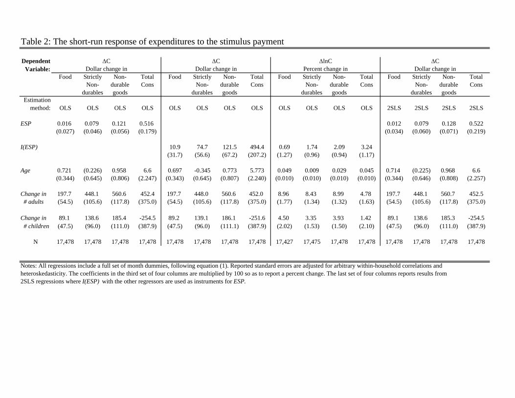
Table 2: The short-run response of expenditures to the stimulus payment

DependentVariable:

Food Strictly Non-

durables

Non-durable goods

TotalCons

Food Strictly Non-

durables

Non-durable goods

TotalCons

Food Strictly Non-

durables

Non-durable goods

TotalCons

Food Strictly Non-

durables

Non-durable goods

TotalCons

Estimationmethod: OLS OLS OLS OLS OLS OLS OLS OLS OLS OLS OLS OLS 2SLS 2SLS 2SLS 2SLS

ESP 0.016 0.079 0.121 0.516 0.012 0.079 0.128 0.522(0.027) (0.046) (0.056) (0.179) (0.034) (0.060) (0.071) (0.219)

I(ESP) 10.9 74.7 121.5 494.4 0.69 1.74 2.09 3.24(31.7) (56.6) (67.2) (207.2) (1.27) (0.96) (0.94) (1.17)

Age 0.721 (0.226) 0.958 6.6 0.697 -0.345 0.773 5.773 0.049 0.009 0.029 0.045 0.714 (0.225) 0.968 6.6(0.344) (0.645) (0.806) (2.247) (0.343) (0.645) (0.807) (2.240) (0.010) (0.010) (0.010) (0.010) (0.344) (0.646) (0.808) (2.257)

Change in 197.7 448.1 560.6 452.4 197.7 448.0 560.6 452.0 8.96 8.43 8.99 4.78 197.7 448.1 560.7 452.5 # adults (54.5) (105.6) (117.8) (375.0) (54.5) (105.6) (117.8) (375.0) (1.77) (1.34) (1.32) (1.63) (54.5) (105.6) (117.8) (375.0)

Change in 89.1 138.6 185.4 -254.5 89.2 139.1 186.1 -251.6 4.50 3.35 3.93 1.42 89.1 138.6 185.3 -254.5 # children (47.5) (96.0) (111.0) (387.9) (47.5) (96.0) (111.1) (387.9) (2.02) (1.53) (1.50) (2.10) (47.5) (96.0) (111.0) (387.9)

N 17,478 17,478 17,478 17,478 17,478 17,478 17,478 17,478 17,427 17,475 17,478 17,478 17,478 17,478 17,478 17,478

Dollar change in

Notes: All regressions include a full set of month dummies, following equation (1). Reported standard errors are adjusted for arbitrary within-household correlations and heteroskedasticity. The coefficients in the third set of four columns are multiplied by 100 so as to report a percent change. The last set of four columns reports results from 2SLS regressions where I(ESP) with the other regressors are used as instruments for ESP.

Dollar change inC

Dollar change inC lnC

Percent change inC

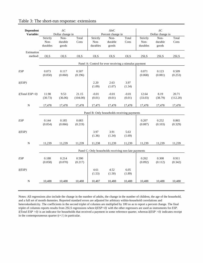
Table 3: The short-run response: extensions

Strictly Non-

durables

Non-durable goods

TotalCons

StrictlyNon-

durables

Non-durable goods

TotalCons

StrictlyNon-

durables

Non-durable goods

TotalCons

Estimation method: OLS OLS OLS OLS OLS OLS 2SLS 2SLS 2SLS

ESP 0.073 0.117 0.507 0.071 0.123 0.509(0.050) (0.060) (0.196) (0.068) (0.081) (0.253)

I(ESP) 2.20 2.63 3.97(1.09) (1.07) (1.34)

I(Total ESP>0) 11.98 9.53 21.15 -0.01 -0.01 -0.01 12.64 8.19 20.71(30.73) (36.06) (104.00) (0.01) (0.01) (0.01) (33.03) (38.79) (112.20)

N 17,478 17,478 17,478 17,475 17,478 17,478 17,478 17,478 17,478

ESP 0.144 0.185 0.683 0.207 0.252 0.865(0.054) (0.066) (0.219) (0.087) (0.103) (0.329)

I(ESP) 3.97 3.91 5.63(1.36) (1.34) (1.69)

N 11,239 11,239 11,239 11,238 11,239 11,239 11,239 11,239 11,239

ESP 0.188 0.214 0.590 0.262 0.308 0.911(0.058) (0.070) (0.217) (0.092) (0.112) (0.342)

I(ESP) 4.61 4.52 6.05(1.53) (1.50) (1.89)

N 10,488 10,488 10,488 10,487 10,488 10,488 10,488 10,488 10,488

Notes: All regressions also include the change in the number of adults, the change in the number of children, the age of the household, and a full set of month dummies. Reported standard errors are adjusted for arbitrary within-household correlations and heteroskedasticity. The coefficients in the second triplet of columns are multiplied by 100 so as to report a percent change. The final triplet of columns reports results from 2SLS regressions where I(ESP>0) with the other regressors are used as instruments for ESP. I(Total ESP >0) is an indicator for households that received a payment in some reference quarter, whereas I(ESP >0) indicates receipt in the contemporaneous quarter (t+1 ) in particular.

Panel B: Only households receiving payments

Panel A: Control for ever receiving a stimulus payment

Panel C: Only households receiving non-late payments

Dependent Variable:

C lnC CDollar change in Percent change in Dollar change in

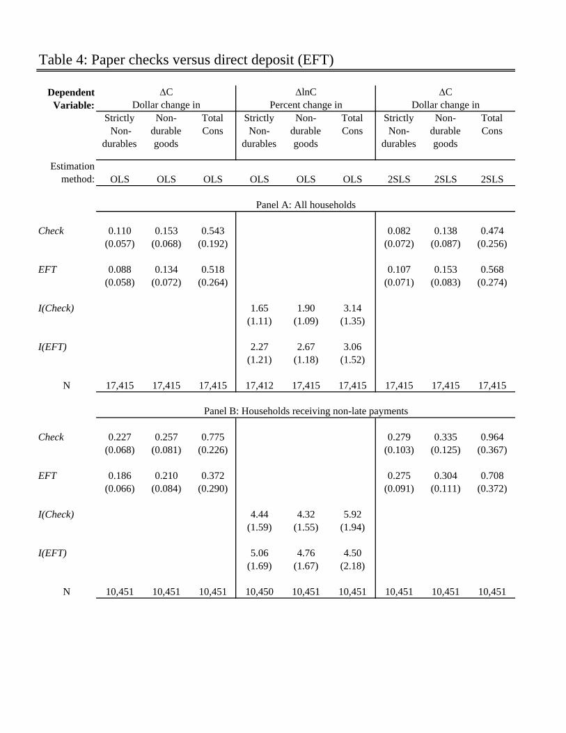
Table 4: Paper checks versus direct deposit (EFT)

Strictly Non-

durables

Non-durable goods

TotalCons

StrictlyNon-

durables

Non-durable goods

TotalCons

StrictlyNon-

durables

Non-durable goods

TotalCons

Estimation method: OLS OLS OLS OLS OLS OLS 2SLS 2SLS 2SLS

Check 0.110 0.153 0.543 0.082 0.138 0.474(0.057) (0.068) (0.192) (0.072) (0.087) (0.256)

EFT 0.088 0.134 0.518 0.107 0.153 0.568(0.058) (0.072) (0.264) (0.071) (0.083) (0.274)

I(Check) 1.65 1.90 3.14(1.11) (1.09) (1.35)

I(EFT) 2.27 2.67 3.06(1.21) (1.18) (1.52)

N 17,415 17,415 17,415 17,412 17,415 17,415 17,415 17,415 17,415

Check 0.227 0.257 0.775 0.279 0.335 0.964(0.068) (0.081) (0.226) (0.103) (0.125) (0.367)

EFT 0.186 0.210 0.372 0.275 0.304 0.708(0.066) (0.084) (0.290) (0.091) (0.111) (0.372)

I(Check) 4.44 4.32 5.92(1.59) (1.55) (1.94)

I(EFT) 5.06 4.76 4.50(1.69) (1.67) (2.18)

N 10,451 10,451 10,451 10,450 10,451 10,451 10,451 10,451 10,451

Panel B: Households receiving non-late payments

Panel A: All households

Dependent Variable:

C lnC CDollar change in Percent change in Dollar change in

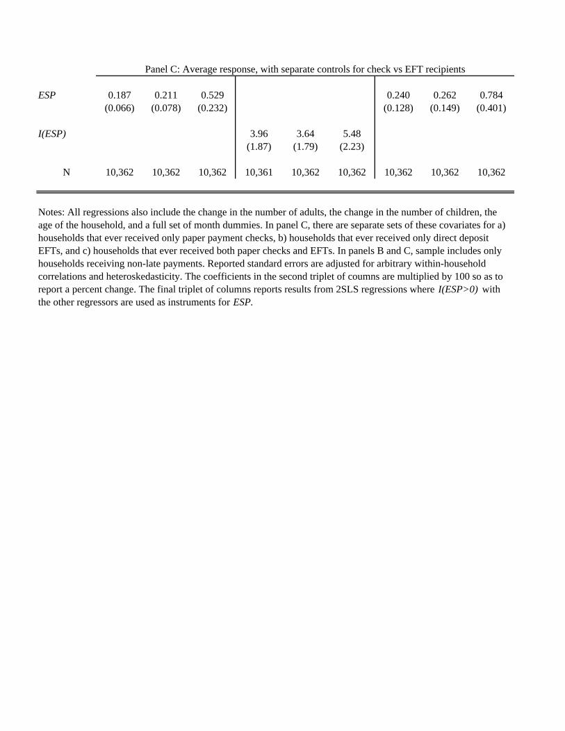
ESP 0.187 0.211 0.529 0.240 0.262 0.784(0.066) (0.078) (0.232) (0.128) (0.149) (0.401)

I(ESP) 3.96 3.64 5.48(1.87) (1.79) (2.23)

N 10,362 10,362 10,362 10,361 10,362 10,362 10,362 10,362 10,362

Panel C: Average response, with separate controls for check vs EFT recipients

Notes: All regressions also include the change in the number of adults, the change in the number of children, the age of the household, and a full set of month dummies. In panel C, there are separate sets of these covariates for a) households that ever received only paper payment checks, b) households that ever received only direct deposit EFTs, and c) households that ever received both paper checks and EFTs. In panels B and C, sample includes only households receiving non-late payments. Reported standard errors are adjusted for arbitrary within-household correlations and heteroskedasticity. The coefficients in the second triplet of coumns are multiplied by 100 so as to report a percent change. The final triplet of columns reports results from 2SLS regressions where I(ESP>0) with the other regressors are used as instruments for ESP.

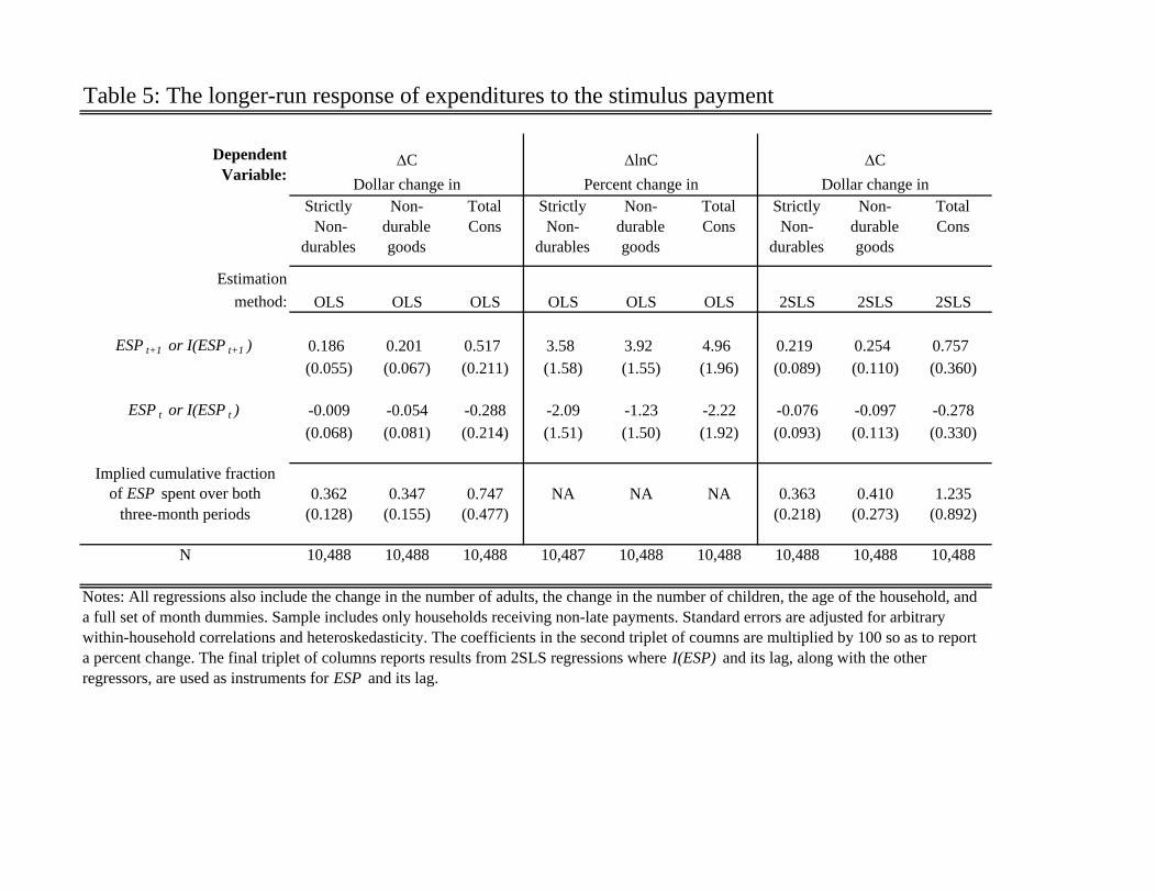
Table 5: The longer-run response of expenditures to the stimulus payment

Strictly Non-

durables

Non-durable goods

TotalCons

StrictlyNon-

durables

Non-durable goods

TotalCons

StrictlyNon-

durables

Non-durable goods

TotalCons

Estimation method: OLS OLS OLS OLS OLS OLS 2SLS 2SLS 2SLS

ESP t+1 or I(ESP t+1 ) 0.186 0.201 0.517 3.58 3.92 4.96 0.219 0.254 0.757(0.055) (0.067) (0.211) (1.58) (1.55) (1.96) (0.089) (0.110) (0.360)

ESP t or I(ESP t ) -0.009 -0.054 -0.288 -2.09 -1.23 -2.22 -0.076 -0.097 -0.278(0.068) (0.081) (0.214) (1.51) (1.50) (1.92) (0.093) (0.113) (0.330)

Implied cumulative fractionof ESP spent over both 0.362 0.347 0.747 NA NA NA 0.363 0.410 1.235

three-month periods (0.128) (0.155) (0.477) (0.218) (0.273) (0.892)

N 10,488 10,488 10,488 10,487 10,488 10,488 10,488 10,488 10,488

CDollar change in Percent change in Dollar change in

Notes: All regressions also include the change in the number of adults, the change in the number of children, the age of the household, and a full set of month dummies. Sample includes only households receiving non-late payments. Standard errors are adjusted for arbitrary within-household correlations and heteroskedasticity. The coefficients in the second triplet of coumns are multiplied by 100 so as to report a percent change. The final triplet of columns reports results from 2SLS regressions where I(ESP) and its lag, along with the other regressors, are used as instruments for ESP and its lag.

Dependent Variable:

C lnC

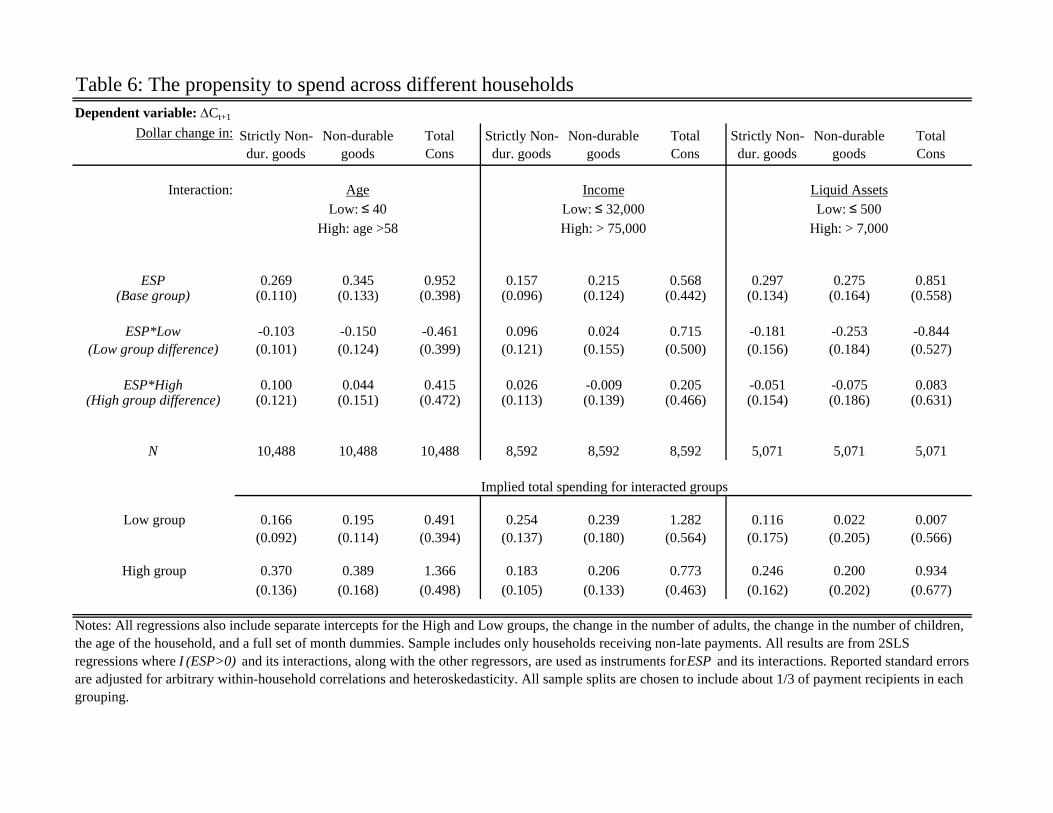
Table 6: The propensity to spend across different households

Dollar change in: Strictly Non-dur. goods

Non-durable goods

TotalCons

Strictly Non-dur. goods

Non-durable goods

TotalCons

Strictly Non-dur. goods

Non-durable goods

TotalCons

Interaction:

ESP 0.269 0.345 0.952 0.157 0.215 0.568 0.297 0.275 0.851(Base group) (0.110) (0.133) (0.398) (0.096) (0.124) (0.442) (0.134) (0.164) (0.558)

ESP*Low -0.103 -0.150 -0.461 0.096 0.024 0.715 -0.181 -0.253 -0.844(Low group difference) (0.101) (0.124) (0.399) (0.121) (0.155) (0.500) (0.156) (0.184) (0.527)

ESP*High 0.100 0.044 0.415 0.026 -0.009 0.205 -0.051 -0.075 0.083(High group difference) (0.121) (0.151) (0.472) (0.113) (0.139) (0.466) (0.154) (0.186) (0.631)

N 10,488 10,488 10,488 8,592 8,592 8,592 5,071 5,071 5,071

Low group 0.166 0.195 0.491 0.254 0.239 1.282 0.116 0.022 0.007(0.092) (0.114) (0.394) (0.137) (0.180) (0.564) (0.175) (0.205) (0.566)

High group 0.370 0.389 1.366 0.183 0.206 0.773 0.246 0.200 0.934(0.136) (0.168) (0.498) (0.105) (0.133) (0.463) (0.162) (0.202) (0.677)

Low: ≤ 40

Dependent variable: Ct+1

Implied total spending for interacted groups

Notes: All regressions also include separate intercepts for the High and Low groups, the change in the number of adults, the change in the number of children, the age of the household, and a full set of month dummies. Sample includes only households receiving non-late payments. All results are from 2SLS regressions where I (ESP>0) and its interactions, along with the other regressors, are used as instruments for ESP and its interactions. Reported standard errors are adjusted for arbitrary within-household correlations and heteroskedasticity. All sample splits are chosen to include about 1/3 of payment recipients in each grouping.

High: age >58

IncomeLow: ≤ 32,000High: > 75,000

Liquid AssetsLow: ≤ 500

High: > 7,000

Age

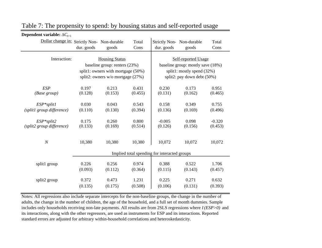
Table 7: The propensity to spend: by housing status and self-reported usage

Dollar change in: Strictly Non-dur. goods

Non-durable goods

TotalCons

Strictly Non-dur. goods

Non-durable goods

TotalCons

Interaction:

ESP 0.197 0.213 0.431 0.230 0.173 0.951(Base group) (0.128) (0.153) (0.455) (0.131) (0.162) (0.465)

ESP*split1 0.030 0.043 0.543 0.158 0.349 0.755(split1 group difference) (0.110) (0.130) (0.394) (0.136) (0.169) (0.496)

ESP*split2 0.175 0.260 0.800 -0.005 0.098 -0.320(split2 group difference) (0.133) (0.169) (0.514) (0.126) (0.156) (0.453)

N 10,380 10,380 10,380 10,072 10,072 10,072

split1 group 0.226 0.256 0.974 0.388 0.522 1.706(0.093) (0.112) (0.364) (0.115) (0.143) (0.457)

split2 group 0.372 0.473 1.231 0.225 0.271 0.632(0.135) (0.175) (0.508) (0.106) (0.131) (0.393)

Housing Status Self-reported Usagebaseline group: renters (23%) baseline group: mostly save (18%)

Dependent variable: Ct+1

split2: owners w/o mortgage (27%)split1: mostly spend (32%)

Implied total spending for interacted groups

Notes: All regressions also include separate intercepts for the non-baseline groups, the change in the number of adults, the change in the number of children, the age of the household, and a full set of month dummies. Sample includes only households receiving non-late payments. All results are from 2SLS regressions where I (ESP>0) and its interactions, along with the other regressors, are used as instruments for ESP and its interactions. Reported standard errors are adjusted for arbitrary within-household correlations and heteroskedasticity.

split2: pay down debt (50%)split1: owners with mortgage (50%)

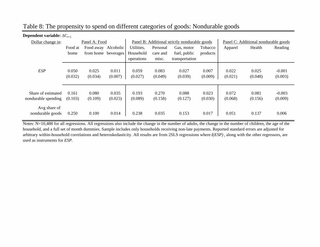
Table 8: The propensity to spend on different categories of goods: Nondurable goodsDependent variable: Ct+1

Dollar change in: Panel A: FoodFood at home

Food away from home

Alcoholic beverages

Utilities, Household operations

Personal care and

misc.

Gas, motor fuel, public

transportation

Tobacco products

Apparel Health Reading

ESP 0.050 0.025 0.011 0.059 0.083 0.027 0.007 0.022 0.025 -0.001(0.032) (0.034) (0.007) (0.027) (0.049) (0.039) (0.009) (0.021) (0.048) (0.003)

Share of estimated 0.161 0.080 0.035 0.193 0.270 0.088 0.023 0.072 0.081 -0.003nondurable spending (0.103) (0.109) (0.023) (0.089) (0.158) (0.127) (0.030) (0.068) (0.156) (0.009)

Avg share of nondurable goods 0.250 0.100 0.014 0.238 0.035 0.153 0.017 0.051 0.137 0.006

Panel C: Additional nondurable goodsPanel B: Additional strictly nondurable goods

Notes: N=10,488 for all regressions. All regressions also include the change in the number of adults, the change in the number of children, the age of the household, and a full set of month dummies. Sample includes only households receiving non-late payments. Reported standard errors are adjusted for arbitrary within-household correlations and heteroskedasticity. All results are from 2SLS regressions where I(ESP) , along with the other regressors, are used as instruments for ESP.

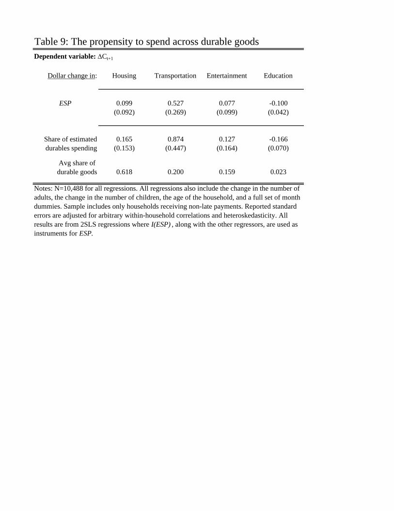
Table 9: The propensity to spend across durable goodsDependent variable: Ct+1

Dollar change in: Housing Transportation Entertainment Education

ESP 0.099 0.527 0.077 -0.100(0.092) (0.269) (0.099) (0.042)

Share of estimated 0.165 0.874 0.127 -0.166durables spending (0.153) (0.447) (0.164) (0.070)

Avg share of durable goods 0.618 0.200 0.159 0.023

Notes: N=10,488 for all regressions. All regressions also include the change in the number of adults, the change in the number of children, the age of the household, and a full set of month dummies. Sample includes only households receiving non-late payments. Reported standard errors are adjusted for arbitrary within-household correlations and heteroskedasticity. All results are from 2SLS regressions where I(ESP) , along with the other regressors, are used as instruments for ESP.