Consumer Price Search and PlatformDesign in Internet Commerce∗

Michael Dinerstein, Liran Einav,

Jonathan Levin, and Neel Sundaresan†

December 2017

Abstract. The platform design–the process that helps potential buyers on the

internet navigate toward products they may purchase–plays a critical role in

reducing search frictions and determining market outcomes. We study a key

trade-off associated with two important roles of efficient platform design–guiding

consumers to their most desired product while also strengthening seller incentives

to lower prices. We use simple theory to illustrate this, and then combine detailed

browsing data from eBay and an equilibrium model of consumer search and price

competition to quantitatively assess this trade-off in the particular context of a

change in eBay’s marketplace design.

∗We thank Greg Lewis, the Editor, three anonymous referees, and many seminar participants for helpfulcomments. We appreciate support from the Alfred P. Sloan Foundation, the National Science Foundation,the Stanford Institute for Economic Policy Research, and the Toulouse Network on Information Technology.Data access for this study was obtained under a contract between Dinerstein, Einav, and Levin and eBayResearch. Neel Sundaresan was an employee of eBay at the time this research began.†Kenneth C. Griffin Department of Economics, University of Chicago (Dinerstein), Department of Eco-

nomics, Stanford University (Einav and Levin), NBER (Dinerstein, Einav, and Levin), and Microsoft(Sundaresan). Email: mdinerstein@uchicago.edu, leinav@stanford.edu, jdlevin@stanford.edu, and nsun-dare@gmail.com.

1 Introduction

Search frictions play an important role in retail markets. They help explain how retailers

maintain positive markups even when they compete to sell near-identical goods, and why

price dispersion is so ubiquitous. In online commerce, the physical costs of search are much

lower than in traditional offline settings. Yet, studies of e-commerce routinely have found

substantial price dispersion (Bailey, 1998; Smith and Brynjolfsson, 2001; Baye, Morgan, and

Scholten, 2004; Einav et al., 2015). One explanation for remaining search frictions in online

markets is that the set of competing products is often very large and changes regularly such

that consumers cannot be expected to consider, or even be aware of, all available products.

To deal with this proliferation of options, consumers shopping online can use either

price search engines or (more often) compare prices at e-commerce marketplaces, or internet

platforms, such as eBay or Amazon. For the most part, these platforms want to limit search

frictions and provide consumers with transparent and low prices (Baye and Morgan, 2001).

Sellers on these platforms may have very different incentives. Many retailers, and certainly

those with no particular cost advantage, would like to differentiate or even “obfuscate” their

offerings to limit price competition (Gabaix and Laibson, 2006; Ellison and Ellison, 2009;

Ellison and Wolitzky, 2012). These often conflicting incentives highlight the important role

of the platform design, which structures online search in a way that affects consumer search

and seller incentives at the same time. In markets where the set of potential offers is large,

the platform’s design may have first-order implications for price levels and the volume of

trade.

In this paper, we use a model of consumer search and price competition to estimate search

frictions and online retail margins, and to study the effects of search design. We estimate the

model using browsing data from eBay. A nice feature of internet data is that it is possible

to track exactly what each consumer sees. As a practical matter, consumers often evaluate

only a handful of products, even when there are many competing sellers. With standard

transaction data, incorporating this requires the introduction of a new latent variable, the

consumer’s “consideration set”; that is, the set of products the consumer actually chooses

between (e.g., Goeree, 2008; Honka et al., 2014). Here, we adopt the consideration set

1

approach, but use browsing data to recover it.

We use the model to estimate consumer demand and retail margins, and then to analyze

a large-scale redesign of the search process on eBay. Prior to the redesign, consumers enter-

ing a search query were shown individual offers drawn from a larger set of potential matches,

ranked according to a relevance algorithm. The redesign broke consumer search into two

steps: first prompting consumers to identify an exact product, then comparing seller listings

of that product head-to-head, ranked (mostly) by price. We discuss in Section 2 how varia-

tions on these two approaches are used by many, if not most, e-commerce platforms, and use

a simple theoretical framework to illustrate the associated trade-offs. In particular, we assess

the trade-off between guiding consumers to their most desired products and strengthening

seller incentives to provide better product attributes. In our empirical context, we focus

on a listing’s quality as fixed in the short-run and price as a flexible product attribute that

sellers can choose. The basic insight applies more generally to any other combination of a

fixed attribute (such as quality) and a flexible attribute that can be changed in the short

run (such as price).

To motivate the analysis, we show in Section 3 that across a fairly broad set of consumer

product categories, re-organizing the search process is associated with both a change in pur-

chasing patterns and a fall in the distribution of posted prices. After the change, transaction

prices fell by roughly 5-15% for many products. We also point out that all of these cate-

gories are characterized by a wide degree of price dispersion, and by difficulties in accurately

classifying and filtering relevant products. Despite a very large number of sellers offering

high-volume products, consumers see only a relatively small fraction of offers, and regularly

do not buy from the lowest-price seller. That is, search frictions appear to be prevalent

despite the low physical search costs associated with internet browsing.

We also present results from a randomized experiment that eBay ran subsequent to

the search redesign. The experiment randomized the default search results presented to

consumers. The experiment results highlight that the impact of the search redesign varies

considerably across product categories that are more homogeneous or less so. It also points

to the limitation of an experiment in testing equilibrium predictions, which may require

longer time and greater scale to materialize and cannot capture equilibrium responses that

2

occur at a level higher than the randomization.

Motivated by these limitations, the primary empirical exercise of the paper proposes a

model of consumer demand and price competition in Section 4, and estimates it in Section 5

for a specific and highly homogeneous product, the Halo Reach video game. We find that even

after incorporating limited search, demand is highly price sensitive, and price elasticities are

on the order of -10. We do find some degree of consumer preference across retailers, especially

for sellers who are “top-rated,” a characteristic that eBay flags conspicuously in the search

process. We also use the model to decompose the sources of seller pricing power into three

sources: variation in seller costs, perceived seller vertical and horizontal differentiation, and

search frictions.

We estimate the model using data on search results, purchase decisions, and posted

prices from before the search redesign plus search results from after the redesign. In Section

6, we apply the model to analyze the search redesign. Despite not using data on purchase

decisions or posted prices from after the redesign, the model can explain, both qualitatively

and quantitatively, many of the effects of the redesign: a reduction in posted prices, a shift

toward lower-priced purchases, and consequently a reduction in transaction prices. The

redesign had the effect of increasing the set of relevant offers exposed to consumers, and

prioritizing low price offers. We find that the latter effect is by far the most important in

terms of increasing price sensitivity and competitive pressure. In fact, we find that under the

redesigned selection algorithm that prioritizes low prices, narrowing the number of listings

shown to buyers tends to increase, rather than decrease, price competition. In contrast, when

we apply the same exercise to a product category that exhibits much greater heterogeneity

across items, prioritizing prices in the search design has negative consequences, and appears

less efficient than search designs that prioritize product quality.

Our paper is related to an important literature on search frictions and price competition

that dates back to Stigler (1961). Recent empirical contributions include Hortacsu and

Syverson (2003), Hong and Shum (2006), and Hortacsu et al. (2012). A number of papers

specifically have tried to assess price dispersion in online markets (e.g., Bailey, 1998; Smith

and Brynjolfsson, 2001; Baye, Morgan, and Scholten, 2004; Einav et al., 2015), to estimate

price elasticities (e.g., Ellison and Ellison, 2009; Einav et al., 2014), or to show that consumer

3

search may be relatively limited (Malmendier and Lee, 2011). Ellison and Ellison (2014)

propose a model to rationalize price dispersion based on sellers having different consumer

arrival rates, and use the model to analyze online and offline prices for used books. Their

model is natural for thinking about consumer search across different websites.

Our paper examines the platform’s role in guiding search specifically in two-sided markets

(Rochet and Tirole, 2006; Rysman, 2009). Lewis and Wang (2013) examine the theoretical

conditions under which reducing search frictions benefits all market participants. Other

theoretical papers have analyzed price discrimination in matching markets (Damiano and

Li, 2007; Johnson, 2013), and while eBay does not price discriminate, its matching rule allows

it to give certain listings higher visibility. Gomes and Pavan (2017) consider a platform both

engaging in second- and third-degree price discrimination and setting a matching rule and

characterize the welfare differences between decentralized markets and centralized markets

mediated by a platform. Empirically, Fradkin (2014) and Horton (2014) are two recent

papers that study search design for internet platforms, in both cases focusing on settings

where there is a rich two-sided matching problem.

2 Search Design in Online Markets

2.1 Conceptual Framework

We begin by describing the simple economics of platform design. Consider J sellers, each

listing one product for sale on a single platform. Each product j (offered by seller j) is

associated with a fixed vector of product attributes xj and is offered for sale at a posted

price pj, which is determined by the seller. Each consumer i who arrives at the platform

is defined by a vector of characteristics ζ i, drawn from a population distribution F . Each

consumer has a unit demand and decides which product to purchase, or not to purchase at

all. Conditional on purchasing product j, consumer i’s utility is given by u(xj, pj; ζ i).

So far we described a standard, traditional setting of demand and supply of differentiated

goods. The distinction, which is the focus of this paper, is the existence of a platform as a

market intermediary, whose main role is in allocating consumers’ attention and/or awareness

4

to different products. This role is less essential in more traditional markets, where the

number of products is limited and consumers are likely to be reasonably familiar with most

of the products. But in online markets, where there are hundreds or sometimes thousands

of different competing products available for sale at a given time, and product churn is high,

consumers cannot be expected to consider, or even be aware of, all these products. This is

the context in which the platform has an important role in deciding which products to make

visible to a given consumer.

A simple generic way to model the platform is by assuming that the platform sets an

awareness/visibility function aij ∈ [0, 1], where aij is the probability that product j is being

considered by consumer i. For example, the platform can decide not to show product j

to anyone, in which case aij = 0 for all i, or can decide to rank order certain products

when it presents search results, which would imply aij > aik for all i iff product j is ranked

higher than product k for all searches. We will consider below the trade-offs associated with

different platform designs where technological or consumer attention generates a constraint

of the form∑

j aij ≤ Ki. To keep things simple, and consistent with the empirical setting

presented below, we further assume that aij = aj = a(pj, xj; p−j, x−j) for all i. That is, the

platform presents products to consumers based on their prices and attributes, but does not

discriminate presentation across consumers.1 The platform charges sellers a transaction fee

T and a fraction t of the transaction price.

Given this setting, platform design implies (possibly stochastic) choice sets, L, for con-

sumers, so that overall demand for product j is given by

Dj(pj, p−j) =∑

L∈2J aLDj(pj, p−j;L), (1)

where

Dj(pj, p−j;L) =∫

1(u(xj, pj; ζ i) ≥ u(xk, pk; ζ i)∀k ∈ L)dF (ζ i) (2)

and

aL =(∏

j∈L aj

)(∏j /∈L(1− aj)

). (3)

1From an ex ante perspective, this still allows for setting 0 < aj < 1, which would be implemented byrandomizing across consumers, and thus generates discrimination ex post.

5

This consideration set approach to modeling demand is not new (see, e.g., Goeree 2008;

Honka et al. 2014); our focus is on the platform’s decision as to how to affect it.2 Note also

that we make the assumption that the platform design affects choices, but does not enter the

consumer’s utility directly; this can be motivated by the fact that conditional on engaging

in a search process, the consumer exerts a fixed amount of effort regardless of the outcome.

Consider now the seller’s pricing decisions. Seller j sets pj to maximize profits

πj = maxpj

Dj(pj, p−j)((1− t)pj − cj − T ), (4)

leading to the familiar first order condition

pj =cj + T

1− t−(∂Dj(pj, p−j)

∂pj

)−1Dj(pj, p−j). (5)

Note that we can write

∂Dj(pj, p−j)

∂pj=∑

L aL∂Dj(pj, p−j;L)

∂pj+∑

L

∂aL∂pj

Dj(pj, p−j;L), (6)

so the price has two distinct effects. One is the usual effect on demand: conditional on

considering product j, consumers are more likely to buy it if its price is lower. The second

effect of price depends on the platform design. If the platform is more likely to show the

product when its price is lower – that is, if∂aj∂pj

< 0 – it provides yet another incentive for

sellers to reduce prices.

This will be a key point that we will focus on throughout the paper. The platform has

two distinct roles in choosing its search design. One is the familiar role of generating more

efficient sorting: trying to help imperfectly informed (or imperfectly attentive) consumers

find their desired product within a large assortment of different products. The second role

of the platform design is to exert stronger pricing incentives on sellers.

Tilting the platform’s design from trying to predict demand for product j towards a

2The literature sometimes draws a distinction between a consumer actively “considering” a product andthe consumer seeing a product but ultimately disregarding it. We will treat a product as part of a consumer’sconsideration set if she is shown the offer, regardless of how seriously she considers it when deciding whetherto purchase. We discuss in Appendix A why our data do not allow us to make such a distinction.

6

design that assigns greater weight to price increases demand elasticities faced by the seller

and maximizes consumer surplus. This is optimal for the platform if its long-run revenues

depend largely on driving consumers to the platform (rather than sellers), which would

be highly correlated with short-run consumer surplus.3 We thus assume that the platform

tries to maximize consumer surplus and use it to determine the optimal platform design.

An alternative would be to model the platform as maximizing short-run profits from the

transaction fee and its cut of the transacted price. The platform’s short-run profits depend

both on the number of transactions and the transacted prices, so the optimal design may

tilt toward assigning greater weight to price, but not as far as maximizing consumer surplus

would. We consider both platform objectives below.

2.2 A Toy Example

We now use this framework to present a highly stylized example, which illustrates some key

elements that will be the focus of the empirical exercise. Consider two products (J = 2),

which are associated with differentiated qualities q1 > q2 such that q1 = q and we normalize

q2 = 0. Corresponding marginal costs are c1 = c and c2 = 0. Consumers have unit demand,

and consumer i’s utility from product j = 1, 2 is given by uij = ζ i + qj − αpj where ζ i

is distributed uniformly on [0, 1], and utility from the outside option for all consumers is

normalized to ui0 = 0. The platform charges the seller T per transaction and keeps fraction

t of the transacted price. We further assume that the platform can only show to consumers a

single product and (as before) cannot discriminate what it shows across consumers. Within

this context, the platform design is reduced to the probability it would show each product,

a1 and a2 = 1− a1, as a function of qualities (q1 and q2) and prices (p1 and p2).

From a seller’s perspective, demand is driven by consumer demand and the platform

3In the context of most e-commerce platforms, including eBay, it seems reasonable to approximate plat-form revenues as a fixed share of transaction volume.

7

strategy:

Dj(pj, p−j) =

aj(pj, p−j) if pj < qj/α

aj(pj, p−j)(1 + qj − αpj) if pj ∈ [qj/α, (1 + qj)/α]

0 if pj > (1 + qj)/α

, (7)

and sellers set prices to maximize profits.

Finally, for illustration, it will also be convenient to assume that the platform cannot

perfectly implement its design strategy (e.g., because there are thousands of products and

quality is estimated/measured, by the platform, with noise). Specifically, we assume that

product 1 is shown to consumers with probability

a1 =[exp (q − βp1)]1/σ

[exp (q − βp1)]1/σ + [exp (−βp2)]1/σ(8)

and product 2 is shown with probability a2 = 1− a1. The platform’s design depends on its

choice of the parameter β ; that is, on the extent to which lower prices are more likely to be

shown to consumers.

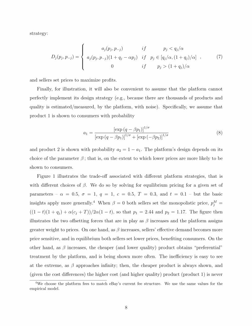
Figure 1 illustrates the trade-off associated with different platform strategies, that is

with different choices of β. We do so by solving for equilibrium pricing for a given set of

parameters – α = 0.5, σ = 1, q = 1, c = 0.5, T = 0.3, and t = 0.1 – but the basic

insights apply more generally.4 When β = 0 both sellers set the monopolistic price, pMj =

((1 − t)(1 + qj) + α(cj + T ))/2α(1 − t), so that p1 = 2.44 and p2 = 1.17. The figure then

illustrates the two offsetting forces that are in play as β increases and the platform assigns

greater weight to prices. On one hand, as β increases, sellers’ effective demand becomes more

price sensitive, and in equilibrium both sellers set lower prices, benefiting consumers. On the

other hand, as β increases, the cheaper (and lower quality) product obtains “preferential”

treatment by the platform, and is being shown more often. The inefficiency is easy to see

at the extreme, as β approaches infinity; then, the cheaper product is always shown, and

(given the cost differences) the higher cost (and higher quality) product (product 1) is never

4We choose the platform fees to match eBay’s current fee structure. We use the same values for theempirical model.

8

shown, which is inefficient. As the bottom left panel of Figure 1 shows, the trade-off is then

resolved with an intermediate value of β (β∗ = 4.11 at the given values of the parameters),

which maximizes consumer surplus. It is important to note that this optimal value of β

is still significantly greater than the corresponding weight assigned to price by consumers

(recall α = 0.5).5

In Figure 2 we use the same setting to illustrate some comparative statics, which are

useful in thinking about the optimal platform design across a range of different product

categories. The top left panel shows how the consumer-surplus optimal platform design, β∗,

varies with the price sensitivity of consumer demand. Naturally, all else equal, as consumers

are more price sensitive (higher α), it is more efficient to increase the importance of price

in the platform design, thus leading to higher β∗. In the top right panel, we show how the

platform design changes with the cost c of the higher quality product. As the cost increases,

the seller of the higher quality product has less ability to mark up its price, so the value to

emphasizing price in the platform design is lower, and β∗ is lower. Similarly, the bottom

left panel shows that as the products are more vertically differentiated, again the optimal

platform design should apply lower weight to price as distorting demand toward the cheaper

product leads to greater inefficiency. In the bottom right panel, we show that as the noise in

measuring quality (σ) increases, the platform design applies a higher weight to price, which

is the product characteristic that can be targeted without error. In Appendix Figure A1

we illustrate similar comparative statics for the platform design that maximizes short-run

platform profits.6

2.3 Existing Approaches to Platform Design

The above framework captures what we view as the two key dimensions of consumer search in

online markets. The first is to try to “predict” consumers’ demand, and guide them toward

5As seen in the bottom right panel of Figure 1, the value of β that maximizes short-run platform profitsis 0.84, which also exceeds α.

6The comparative statics for q and σ are similar to Figure 2. For small levels of price sensitivity (α),βπ∗ = 0 as the platform benefits from a high transacted prices while consumer surplus does not significantlyfall. But for higher levels of price sensitivity, βπ∗ is increasing in α. For small levels of the cost c of thehigher quality product, βπ∗ is increasing in c; for higher levels of c, the higher quality products is less likelyto be shown and then βπ∗ = 0.

9

relevant products, either in response to a user query, or through advertising or product

recommendations. The second is to help consumers find a retailer offering an attractive price

for a product the consumer desires, and by doing so amplify the effective price elasticity faced

by sellers. Empirically, due to different consumer mix and different product offering, online

platforms adopt heterogeneous approaches to the search problem by emphasizing one of the

above dimensions, or both.

Platforms have to identify a relevant set of offers, and present the information to con-

sumers. Identifying relevant offers is easier when products have well-defined SKUs or catalog

numbers (in the context of the model, this can be thought of as a case with relatively low

σ). But as we will note below, it is still a difficult problem for platforms that have tens of

thousands of different listed products. Platforms also take different approaches to presenting

information. A typical consideration is whether to try to present all the relevant products

in a single ordered list that attempts to prioritize items of highest interest, or try to classify

products into sets of “identical” products, and then order products within each set based on

price or other vertical attributes.

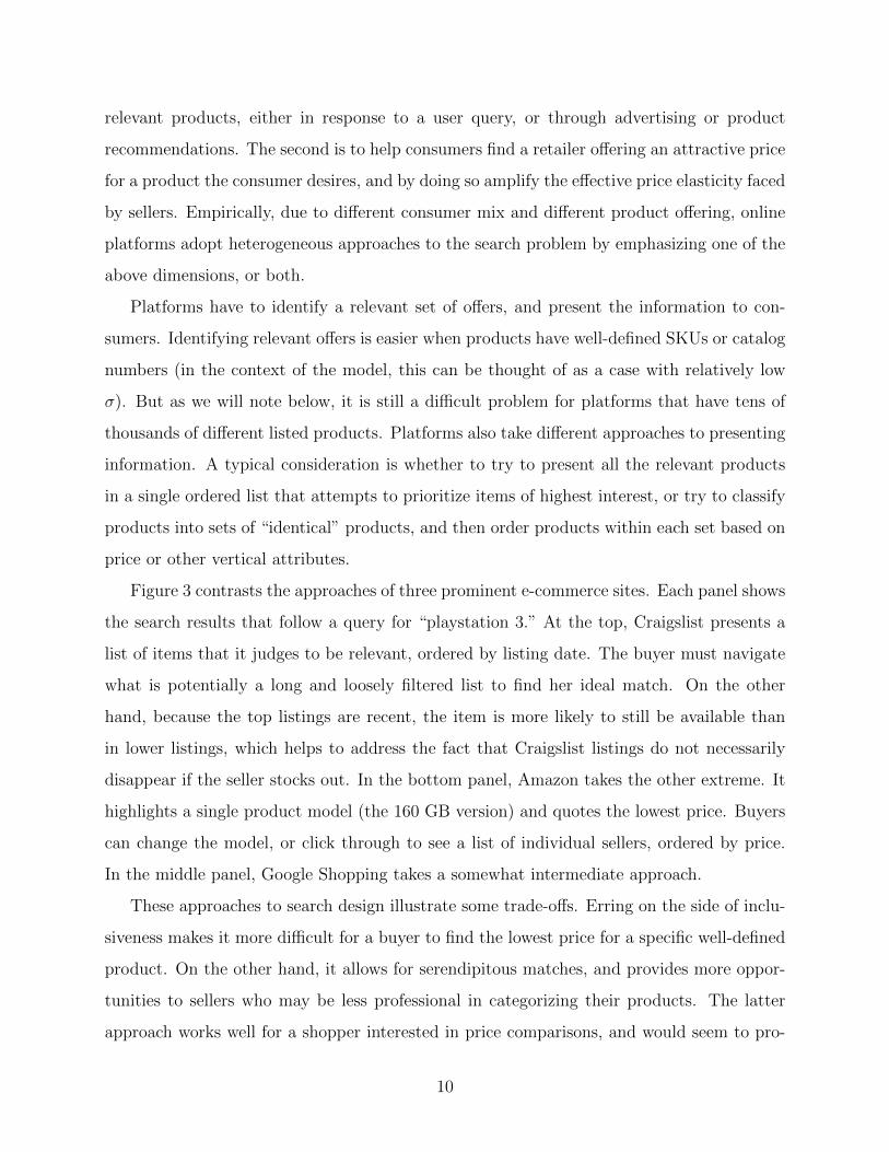
Figure 3 contrasts the approaches of three prominent e-commerce sites. Each panel shows

the search results that follow a query for “playstation 3.” At the top, Craigslist presents a

list of items that it judges to be relevant, ordered by listing date. The buyer must navigate

what is potentially a long and loosely filtered list to find her ideal match. On the other

hand, because the top listings are recent, the item is more likely to still be available than

in lower listings, which helps to address the fact that Craigslist listings do not necessarily

disappear if the seller stocks out. In the bottom panel, Amazon takes the other extreme. It

highlights a single product model (the 160 GB version) and quotes the lowest price. Buyers

can change the model, or click through to see a list of individual sellers, ordered by price.

In the middle panel, Google Shopping takes a somewhat intermediate approach.

These approaches to search design illustrate some trade-offs. Erring on the side of inclu-

siveness makes it more difficult for a buyer to find the lowest price for a specific well-defined

product. On the other hand, it allows for serendipitous matches, and provides more oppor-

tunities to sellers who may be less professional in categorizing their products. The latter

approach works well for a shopper interested in price comparisons, and would seem to pro-

10

mote price competition, provided that the platform is able to accurately identify and classify

listings according to the product being offered. At the same time, as Ellison and Ellison

(2009) have highlighted, it may provide sellers with a strong incentive to search for unpro-

ductive tactics that avoid head-to-head price competition.

3 Setting and Motivating Evidence

3.1 Background: Changes in Platform Design on eBay

With this general framework in mind, the rest of the paper will use detailed data from eBay,

taking advantage of an interesting episode of platform design changes to eBay’s marketplace,

which allows us to compare the different approaches. Appendix B provides more details about

the data construction.

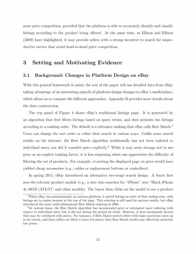
The top panel of Figure 4 shows eBay’s traditional listings page. It is generated by

an algorithm that first filters listings based on query terms, and then presents the listings

according to a ranking order. The default is a relevance ranking that eBay calls Best Match.7

Users can change the sort order or refine their search in various ways. Unlike some search

results on the internet, the Best Match algorithm traditionally has not been tailored to

individual users, nor did it consider price explicitly.8 While it may seem strange not to use

price as an explicit ranking factor, it is less surprising when one appreciates the difficulty of

filtering the set of products. For example, re-sorting the displayed page on price would have

yielded cheap accessories (e.g., cables or replacement buttons or controllers).

In spring 2011, eBay introduced an alternative two-stage search design. A buyer first

sees the relevant product models (e.g., a user who searches for “iPhone” sees “Black iPhone

4s 16GB (AT&T)” and other models). The buyer then clicks on the model to see a product

7When eBay was predominantly an auction platform, it sorted listings in order of their ending time, withlistings set to expire soonest at the top of the page. This ordering is still used for auction results, but eBayintroduced the more multi-dimensional Best Match ordering in 2008.

8At various times, the Best Match algorithm has incorporated price or attempted more tailoring withrespect to individual users, but it did not during the period we study. However, it does incorporate factorsthat may be correlated with prices. For instance, if Best Match moved sellers with high conversion rates upin the search, and these sellers are likely to have low prices, then Best Match results may effectively prioritizelow prices.

11

page with specific listings, shown in the bottom panel of Figure 4.9 The product page has

a prominent “Buy Box” that displays the seller with the lowest posted price (plus shipping)

among those reputed sellers who are classified as “top rated” by eBay.10 Then there are two

columns of listings, one for auctions and one for posted prices. The posted price listings are

ranked in order of price plus shipping (and the first listing may be cheaper than the Buy

Box if the lowest-price seller is not top-rated). The auction listings are ranked so that the

auction ending soonest is on top. We will not focus on auctions, which represent 33% of

the transactions for the products on which we focus. The two designs correspond closely to

the cases we considered in our stylized example of Section 2.2. The Best Match algorithm

incorporated only non-price product characteristics into the ordering of search results, which

is analogous to setting β = 0 in our example, while the product page ordered fixed price

listings based only on price, which is analogous to setting β to be quite high.

About a year later, however, in summer 2012, eBay evaluated the redesign with an

experiment in which users were randomly assigned to be shown either product page or Best

Match results in response to a search query (or more precisely, to search queries for which

a product page existed).11 The experiment, which we were not involved in, was run on 20

percent of the site’s traffic. After being shown initial results using the randomized type of

results page as a default, users could choose to browse using the other type of results page.

So whereas the initial redesign introduced the product page and steered users toward it, the

experiment tested whether conditional on both types of results being available, it was better

to start users with relevance results. Subsequent to the experiment, eBay made the original,

Best Match results the default view for searchers.12

While much of our analysis below will focus on the initial, 2011 changes, we also report

the main patterns that emerge from the subsequent, 2012 experiment.

9The concept of a product page existed on eBay earlier, but its design was very different and it wasdifficult to find, so that only a small minority of users ever viewed it.

10To become a top-rated seller on eBay.com in 2011, a seller needed at least 1,000 transactions and $3,000in sales over the previous 12 months and a positive feedback score above 98%.

11The randomization occurred at the level of a user session. A user session ends if the browser is closedor the user is inactive for at least 30 minutes. Users with customized search preferences, such as preferringresults sorted by shipping distance, were not affected by the experiment.

12The search design has continued to evolve, but the default search results continue to be a Best Matchrelevance ranking, albeit one that it likely to be correlated with price for well-defined products.

12

3.2 The Impact of The Product Page: Descriptive Evidence

The new product page was introduced on May 19, 2011.13 However, the traditional search

results page remained the default view for buyers. The new product page became the

default presentation of search results for five large categories — cell phones, digital cameras,

textbooks, video games, and video game systems — over a one-week period from June 27,

2011 to July 2, 2011. The traditional Best Match results were still accessible to buyers, so

the best way to view the change is probably to think of buyers as now having access to two

types of search results, and being nudged toward (and defaulted into) the product page.

Appendix Figure A2 provides a timeline of the platform changes.

Table 1 shows statistics for these five categories in the period before the product page

was introduced (April 6 to May 18) and the period after the introduction was completed

(August 1 to September 20). We drop the intermediate period during which the product

page was available, but not the default. We also exclude the month of July to allow time for

sellers to respond to the platform redesign. The sample period covers nearly half a year, so

one potential concern is that there may have been changes in the set of products available,

especially in the categories with shorter product life cycles. To deal with this, we restrict

attention to the ten products in each category that were most commonly transacted in the

week before the product page became the default. As an example, a typical product in the

cell phone category is the black, 16GB iPhone 4 for use with AT&T. We also show statistics

for the narrower product category of iPhone 4.

Several patterns are clear in the data. There are many listings for each product. The

average number of listings ranges from 16 to 41 across the five categories. There is also

remarkable variation in prices. The average ratio of the 75th percentile price to the 25th

percentile price is 1.22 in cell phones, 1.32 in digital cameras, and higher in the other cate-

gories. The extreme prices, especially on the high end, are even more dramatic. Consumers

generally do not purchase at the lowest price. In the period before the redesign the average

purchase price often was around the 25-40th percentile of the price distribution. As an ex-

ample, in the digital camera category, consumers pay on average around 18% more than if

13eBay ran a small pilot in September 2010 and implemented the product page for the GPS, DVD, andMP3 categories. These categories are not included in our subsequent analyses.

13

they had selected the 10th percentile price.

The comparison between the two periods is also informative. With one exception (video

game systems), transacted prices fell in every category after the new product page was

introduced. The fall was relatively small in the cell phone and video game categories (2.1%

and 7.7%, respectively), and larger in digital cameras and textbooks (15.7% and 15.9%).

The decrease does not appear to be driven by a general time trend. The qualitative results

remain similar when we control for product-specific (linear) time trends. In part, the drop

in transacted prices reflects a fall in the posted prices that were being offered. Posted prices

fell in every category (again, with the exception of video game systems), by between 0.9%

and 17.7%, demonstrating the redesign’s long-run effect on seller pricing.

Several statistics are suggestive of changes in which listings consumers considered. In

every category except one, consumers after the redesign purchased items that were cheaper

relative to the current distribution of prices. The share of purchases from top-rated sellers

also increased markedly for many of the products. Both of these results seem fairly natural.

The redesigned search selects and sorts listings by price, focusing attention on the low-price

offers, and the product page Buy Box especially promotes the low-priced Top-Rated Seller

(TRS).14

Figure 5 presents a final piece of descriptive evidence, that is also consistent with a change

in consumer search patterns after the redesign. The figure is constructed using browsing data

for a single product, the video game Halo Reach, which we will use to estimate our model

below. The top panel shows the distribution of new, fixed price Halo Reach offers that were

displayed to each consumer following a targeted search, before and after the change in the

search design. The size of the consumer “consideration set” increased sharply. The second

panel shows the distribution of the total number of clicks made in a browsing session, for

consumers who ended up purchasing a new, fixed price Halo Reach video game listing. After

the search redesign, consumers generally clicked fewer times on their way to a purchase,

consistent with a more streamlined process.

14As mentioned, we focus on the August-September “After” period, because it seemed plausible that theeffect of the change on seller’s pricing may take some time to play out. The July results are generallyintermediate, with most of the change in TRS transactions and price percentile occurring immediately.

14

3.3 Moving Back to Traditional Best Match: Results from eBay’s

Experiment

As the stylized example in Section 2.2 highlights, the effects of platform design likely de-

pend on the product’s degree of quality differentiation, q. The experiment provides a clean

comparison of demand behavior under the different platform designs. Note, however, that

because the two designs were simultaneously active and sellers set a single price per listing,

the experiment will not induce any differential changes to pricing incentives. Therefore, the

experimental results will only capture the platform’s ability to efficiently sort consumers to

listings and not its effect on pricing. We will return to this shortcoming in the next section.

We first examine the experiment’s average results, aggregating across all product cate-

gories. A starting point is that the experiment did succeed in steering users toward particular

results. For users randomly assigned to the product page by default, 3.45% of all sessions

included a product page visit, compared to 1.87% for users who were randomly assigned to

the Best Match default. A straight comparison of the two user groups, focusing on products

for which the product page was feasible, showed that the Best Match group had a higher

purchase rate: 0.280% versus 0.267%, with a t-statistic of 10.75 on the difference. The Best

Match group also had slightly higher average transacted prices: $53.35 versus $52.23, with

the difference being only marginally significant (t-stat of 1.85). As mentioned, this compar-

ison made eBay make the traditional Best Match results the default view for searchers.

The higher purchase rate for the Best Match group (despite slightly higher average prices

paid) suggests that non-price characteristics play an important role. To explore further, we

collected data on all purchases from the experimental user sessions, for the period July 25,

2012 to August 30, 2012. We restrict attention to the 200 products with product pages that

were visited at least 1,000 times and had at least 20 purchases during the experiment, and

to fixed price listings for these products.

Following our earlier discussion, we conjectured that relevance ranking might have been

particularly effective for differentiated products, where consumers may care about features

other than price. We therefore construct a proxy for each product’s level of homogeneity.

We use the fact that when a seller posts a new listing, eBay often suggests a title based

15

on the product code. We take the fraction of product listings with the most common (i.e.

suggested) title as a measure of product homogeneity.15

Figure 6 reports statistics based on this cut of the experimental data. The top panel

shows, by product, the price effect of making the Best Match the default search results

page relative to making the Product Page the default. The bottom panel shows the same

for quantity. The effect is highly heterogeneous across products, presumably reflecting a

combination of sampling variation and idiosyncrasies across products in how much residual

heterogeneity across listings exists. Overall, while the average price and quantity effects

are both small, but positive, there is a remarkable variation across products, with products

that are more heterogeneous having the greatest (and non-trivial) positive quantity and

price effect when Best Match is used, while more homogeneous products are associated with

essentially no quantity effect and a slight negative price effect due to Best Match.

3.4 Discussion

The results in Section 3.2 provide a descriptive and qualitative sense of the overall effects of

the platform change. After the change, transaction prices fell for many products. This ap-

pears to have resulted from both a change in purchasing patterns and a fall in the distribution

of posted prices. The experiment results (reported in Section 3.3) highlight the important

heterogeneity in this response across products, even within a fairly narrow product category.

The estimated heterogeneous effects confirm that the platform’s trade-off between prioritiz-

ing price or non-price characteristics depends closely on the product’s level of differentiation.

Taken together, the collection of descriptive results reported in this section suggests that the

platform design is an important feature of the eBay market, and that platform changes could

make a non-trivial difference for market outcomes. At the same time, while the patterns are

suggestive regarding some of the channels that are in play, the analysis also highlights the

difficulties in interpreting the empirical patterns without a model.

15Implicitly the idea we have in mind is that for a more heterogeneous product, say with accessories orslightly different specifications, the seller would need to modify the title. Sellers might also modify the titleas a way to create perceived heterogeneity. We also tried constructing a Herfindahl index based on the listingshares of different titles for each product, and obtained similar types of results to what we report below. Forour empirical model, we will construct a more direct measure of listing quality. The measure will rely onextensive search results data and thus is not practical for analysis across many products.

16

Consider the results from the experiment first in light of the empirical framework pre-

sented in Section 2. The premise of the framework is that pricing on the platform responds

to the platform design, yet the experiment, while useful in highlighting the importance of

heterogeneity across products, cannot capture this pricing response for two reasons. First,

sellers respond to their expected demand, and the experiment affected only a small share

of users. Furthermore, expected demand is integrated over users reaching both types of

search results, so we cannot compare across experimental groups. Second, sellers’ pricing

decision and strategies are unlikely to respond immediately, so although the short run re-

sponse (captured in the results presented earlier) might be indicative of the longer run effects,

quantitatively it could be quite different. On the other hand, the results suggest that het-

erogeneity across products appears to be quite important, and this may make it difficult to

interpret the category-average patterns we presented in Section 3.2.

Therefore, in the next section we develop and estimate a more complete model of the

underlying economic primitives. The model allows us to explain the price levels and the

purchasing patterns in the data, and separate the demand and pricing incentive effects of

the platform change, as well as to evaluate alternative platform changes and product types

not present in the data.

4 An Empirical Model

In this section, we describe a model of consumer search and price competition. In the next

section, we estimate the model’s parameters using data from a single product market, and use

the estimates to quantify search frictions, the importance of retailer and listing heterogeneity,

the size of retailer margins, and the way that the platform redesign affected all of these.

The model’s ingredients are fairly standard. Each potential buyer considers a specific

and limited set of products. He or she then chooses the most preferred. This is modeled as

a traditional discrete choice problem. Sellers set prices in a Nash Equilibrium, taking into

account buyer demand. The role of the platform is to shape consumer search. Rather than

considering all available products, consumers consider the ones suggested by the platform.

We take advantage of detailed browsing histories to explicitly collect data on each buyer’s

17

consideration set. In this context, search rankings affect the set of considered products, and

hence consumer choices, and indirectly, the incentives for price competition.

4.1 Consumer Demand

We consider a market in which, at a given point in time, there are a large number of different

sellers offering either the targeted or a non-targeted product. The targeted product is the

product that is the focus of the market (e.g., the product corresponding to the search terms

the user specifies) while non-targeted products are other, possibly-related products. We

allow listings to vary only by their price p, vertical quality q,16 and by whether they are

listed by a top-rated seller (denoted TRS). We attribute any additional differentiation to

a logit error. We assume that consumer i’s utility from listing j of the targeted product is

given by

uij = α0 + α1pj + α2TRSj + α3pjTRSj + α4qj + εij, (9)

where εij is distributed Type I extreme value and is independent of the listing’s price, quality,

and TRS status.

We assume that consumer i’s utility from listing m of the non-targeted product is given

by

uim = δ + λεim, (10)

where εim is independently distributed Type I extreme value. We parameterize the degree

of horizontal differentiation of non-targeted products by λ to allow non-targeted products to

be more or less differentiated than targeted products.17

The main distinction of the model comes in analyzing the consideration set. The consid-

eration set is denoted by Ji, such that Ji ⊆ J , where J is the set of all available offerings on

the platform. Let JJi and JMi denote the set of targeted and non-targeted listings, respec-

tively, in the consideration set. We assume that the outside good, good 0, which represents

either not buying the product or buying it via another sales channel or by auction, is also

part of the consideration set. It has utility ui0 = εi0, where εi0 is also an independent Type

16We describe the way we measure quality in the next section.17This parameterization yields the same substitution patterns across the non-targeted and targeted prod-

ucts as a nested logit.

18

I extreme value random variable. Consumers choose the utility-maximizing option in their

consideration set.

To estimate the demand parameters, we rely on our browsing data to identify the consid-

eration sets of a large sample of buyers, and their resulting choices. Specifically, we assume

the consideration set includes all the listings on the page seen by the consumer following

his last search query. This is usually the listings page prior to the platform redesign, and

the product page afterwards. With an observable consideration set for each buyer, demand

estimation is straightforward using the familiar multinomial logit choice probabilities.18

4.2 Consideration Sets

In order to analyze pricing decisions, and make out-of-sample predictions, we also develop a

simple econometric model of how consideration sets are formed. To do this, we assume that

consumer i observes the offers of Li = (LJi , LMi ) sellers, where Li is random. We estimate its

distribution directly from the data, that is, by measuring the frequency with which observed

consideration sets include a given number of targeted and non-targeted listings. We assume

that Li, the number of the items in the consideration set, is independent of any particular

buyer characteristics, or the distribution of prices.

Which listings of the targeted product make it into the consideration set? Prior to the

redesign, we noted that price did not factor directly into search ranking, but that after the

redesign, it played a predominant role. In practice, the complexity of the search ranking and

filtering algorithms, which must be general enough to work for every possible search query

and product, as well as factors such as which server provides the results, adds less purposeful

(and perhaps unintentional) elements to what results are shown.

To capture this, we adopt a stochastic model of how listings are selected onto the displayed

page. Specifically, we assume that products are sampled from the set of available targeted

products Ji, such that each product j ∈ Ji is associated with a sampling weight of ωj.

18We leverage our extensive browsing data to treat consideration sets as observable rather than latent. Bytreating consideration sets as a platform choice, our model and counterfactual results abstract away fromforms of consumer search beyond typing in the initial search terms and considering every listing on theresults page. As discussed in Appendix A, searchers rarely click on multiple listings such that the alternativeof treating the consideration set as the set of products clicked on loses important information.

19

Before the redesign, we assume the sampling weight equals the listing’s quality, qj. While a

listing’s quality may be correlated with its price, it is fixed and thus price changes do not

affect the listing’s sampling weight. This reflects eBay’s use of the Best Match algorithm,

which attempts to rank listings based on a single-dimensional measure of a listing’s quality.

This model therefore allows us to use browsing data from before the redesign to infer listings’

quality, which we then use in our demand estimation.

After the redesign, listing j’s sampling weight is

ωj = exp

[−γ

(pj −mink∈J J

i(pk)

stdk∈J Ji

(pk)

)]. (11)

Consumer i’s consideration set is then constructed by sampling LJi products from J Ji , with-

out replacement. This implies that the consideration set of targeted listings is drawn from

a Wallenius’ non-central hypergeometric distribution. We expect γ > 0 so that lower price

items are disproportionately selected into the consideration set after the platform redesign.

We further modify the sampling process after the redesign to incorporate a Buy Box by

reserving one position in the consideration set for a TRS product. Specifically, we draw

the first product in the consideration set from the set of available targeted products from

TRS sellers, J TRS,Ji . Denote this product j0i . We then draw the remaining LJi − 1 products

from J Ji \j0i , without replacement. Below we estimate q and γ using the browsing data that

records the listings that appeared on pages buyers actually visited.

4.3 Pricing Behavior

We model sellers as pricing using a standard Nash Equilibrium assumption.19 Facing the

platform’s transaction fee T and ad valorem fee t, seller j of a targeted product with marginal

19In our data, the modal seller is associated with a single listing. For simplicity, even for sellers who sellmultiple items, we assume that prices are set for each listing independently. This assumption is unlikelyto affect the results much given that the large number of sellers and products make it unlikely buyers aresubstituting across listings of the same seller. In 98.6% of the pre-redesign search sessions, all listings comefrom different sellers.

20

cost cj sets its price to solve

maxpj

((1− t)pj − cj − T )Dj(pj). (12)

Here Dj(pj) is the probability a given buyer at period t selects j’s product, given the set

of offerings J . From a seller’s perspective, Dj(pj) depends on how consumers form their

consideration sets, as well as the choices they make given their options. Using the logit

choice probabilities, we have

Dj(pj) =∑

J : j∈J⊆J

exp (α0 + α1pj + α2TRSj + α3pjTRSj + α4qj)

1 + exp (δ + λ ln |JM |) +∑

k∈JJ exp

α0 + α1pk + α2TRSk+

+α3pkTRSk + α4qk

Pr (J |J ) .

(13)

Another important consideration here is the set (J ) of competing items that the seller has

in mind when it sets its price. We assume that the seller optimizes against the (stochastic)

set of competing products over the entire lifetime of the listing. The competing items are

drawn from the approximately one month (either “before” or “after”) period considered.

When a competing listing is simulated to be purchased, it is replaced on the site by another

listing from the period.20 See Backus and Lewis (2016) for related work on stochastic sets

of competing products.

To understand the seller’s pricing incentives, it is useful to write Dj (pj;TRSj, qj) =

Aj (pj;TRSj, qj)Qj (pj;TRSj, qj), where Aj is the probability that the listing enters the

consideration set given pj and J , and Qj is the probability that the consumer purchases

item j conditional on being in the consideration set. With this notation, the optimal price

pj satisfies:

pjcj

=

(1 +

1

ηD

)−1=

(1 +

1

ηA + ηQ

)−1, (14)

20The new listing that replaces the purchased one is sampled according to the length of time the listingswere actually active on eBay during our estimation period. Thus, sellers are more likely to face competitorswho are selling many units at once or competitors with relatively unattractive products as they remain onthe simulated site for longer. Every 100 searches we exogenously reset the set of competing products toaccount for the feature that some eBay listings expire without being purchased.

21

where ηD, ηA, ηQ are respective price elasticities.21 When γ > 0, reducing price increases

demand in two ways: by making it more likely that the seller ends up in the consideration set

(ηA < 0) and by making it more likely that the consumer picks the seller, conditional on the

seller being in the choice set (ηQ < 0). Increasing γ intensifies the first effect. In addition,

increasing γ effectively faces each seller with tougher competition conditional on making it

into the consideration set, by reducing the likely prices of the other sellers who are selected.

4.4 Discussion

The model we have chosen has only a handful of parameters. A main reason is that we wanted

something easy to estimate and potentially “portable” across products, but yet with enough

richness to be interesting. In Appendix A we report results from a much richer consumer

search model, which more explicitly models the decision of how to search, and which item to

click, before a final purchase decision is made. As we discuss in Appendix A, the estimated

model described above can be viewed as a more general demand framework, which captures

some of the key elasticities that affect the platform design using free parameters, while

summarizing many other components of the consumer search process in a reduced form.

The assumptions we have chosen relate fairly closely to some of the classic search models

in the literature. For example, in Stahl’s (1989) model there are two types of consumers:

consumers who (optimally) sample a single offer completely at random, and consumers who

sample all the offers. This corresponds to having L ∈ {1, |J |} and γ = 0. Stahl’s model

has no product differentiation and the pricing equilibrium is in mixed strategies, but it has

very intuitive properties. For instance, if more consumers have L = 1, equilibrium prices are

higher. Consideration set sizes have the same effect in our model with γ = 0. The same need

not be true with γ > 0. For instance, suppose that sellers have identical cost and quality

and none are top-rated. As γ → ∞, consideration sets are selected purely on the basis of

price. Then having L = 1 for all consumers creates perfect Bertrand competition, whereas

if L = |J | we have a symmetric logit demand model with consequent markups.

There are several obvious directions in which our model can be extended and we have

21To see this, note that ηD = D′(p/D), D = AQ, and D′ = Q′A+A′Q. This implies that ηD = D′(p/D) =Q′(p/Q) +A′(p/A) = ηQ + ηA.

22

explored some of them. One is to allow for more heterogeneity among consumers. It might be

interesting to distinguish between price-elastic “searchers” and price-inelastic “convenience”

shoppers, as in Stahl (1989) or Ellison (2005). We also have not focused on search rank. In

their study of a price search engine, Ellison and Ellison (2009) find page order, especially

first position, to be very important, and it is perceived to be very important in sponsored

search advertising. We have estimated versions of our model that include page order, but

decided not to focus on these versions. One reason is that the effect of page order in our data

seems to be far less dramatic than in sponsored search. The estimates also are much harder

to interpret, a significant drawback given the modest increase in explanatory power.22

5 Estimation and Results

5.1 Estimation Sample

To estimate the model, we focus on a single, well-defined product: the popular Microsoft

Xbox 360 video game, Halo Reach. This video game is one in a series of Halo video games.

It was released in September 2010. Microsoft originally set an official list price of $59.99,

which it shortly dropped to $39.99. We chose this specific game because a large number of

units transact on eBay, and because it had a relatively stable supply and demand during our

observation period of Spring-Summer 2011. The prices of many consumer electronics on the

platform exhibit a time trend, usually starting high and falling quickly over the product life

cycle. Others have a range of characteristics that vary across listings, complicating demand

and supply estimation. In fact, 51% of Halo Reach listings share the same title, our proxy for

degree of product homogeneity when we compared products from the experiments in Section

3. This places Halo Reach at the 82nd percentile for product homogeneity.

The Halo Reach video game is a fairly homogeneous product. It would have been interest-

ing to compare and contrast results from this product against a less homogeneous product,

but once a product becomes heterogeneous the challenge faced by the platform immediately

22One reason for this is that, to the extent that rank and price are correlated, it is somewhat challengingto identify the two terms separately. Another issue is that pages tend to include many non-targeted items(accessories, etc.) as well as auctions, which makes for many complicated modeling decisions in terms ofwhether to include absolute rank, or relative rank among targeted listings, or some mixture of the two.

23

translates to two challenges faced by the researcher: identifying the set of listings that would

be classified as such a product and identifying the set of search terms that capture most

potential buyers of the product. Instead, we therefore use the counterfactual exercise as way

to quantitatively assess the tradeoff.

The data for the analysis come directly from eBay and are described in more detail in

Appendix B. They include all listing-level characteristics as well as individual user searches.

We can observe every aspect of the search process, including what the user saw and her

actions. We use data from two periods: the “before” period from April 6 until May 18, 2011,

and the “after” period, which we define to be August 1 until September 20, 2011.23 The

search data consist of all visits to the Halo Reach product page as well as all visits to the

standard search results page derived from query terms that include the words “xbox” (or

“x-box”), “halo,” and “reach.” This results in 14, 753 visits to the search results page (9, 409

of them in the pre-period) and 6, 733 visits to the product page (18 in the pre-period).24

As search results often include extraneous results while the product page only shows

items that are listed under “Halo Reach” in eBay’s catalog, we identify listings as the Halo

Reach video game if eBay catalogued them as such. We also visually inspected each listing’s

title to verify that the listing is for just the video game. Illustrating the difficulty of precisely

filtering listings, even after we restrict attention to listings catalogued as Halo Reach, we

found that 12% of listings were not Halo Reach-related, and 33% were not the game itself

(e.g., they were accessories). We define “targeted listings” as new Halo Reach items, listed

either with a posted price, or as an auction but with a Buy-It-Now price.25 The non-targeted

fixed price listings are those that appear in search results but do not meet our definition of

targeted because they are used items or are not the Halo Reach video game itself.

Finally, sellers are allowed to change a listing’s price even after it has been listed. When

23As before, we drop July 2-31, 2011 when the product page was the default because our descriptiveanalysis in Section 3 suggested that price adjustment did not happen immediately and we want to use anequilibrium model for prediction. The predictive fit is similar for demand if we include July, and a bit worsefor pricing.

24The “product page” in the pre-period was more rudimentary than one introduced on May 19 (see footnote9), and relatively few people navigated to it.

25According to eBay, “new” items must be unopened and usually still have the manufacturer’s sealing ororiginal shrink wrap. The auction listings with a Buy-It-Now price have a posted price that is available untilthe first bid has been made. We only consider these listings during the period prior to the first bid.

24

this happens, we always observe whether there has been a price change, and we observe the

price if there was a transaction, or if a user in our search data clicked on the item, or if it

was the final posted price of the listing. This leaves a relatively small number of cases where

we have a listing for which we know the price was changed but do not observe the exact

price because the listing was ignored during this period.26

5.2 Descriptive Statistics

Table 2 reports summary statistics for the before and after periods. The numbers of sellers

and listings are slightly lower in the after period, and more of the listings come from top-

rated sellers. These differences, particularly the increase in top-rated seller listings, could

be a consequence of the platform change. In addition, the mean and median list prices both

drop by about $2 in the after period, which is consistent with the earlier results on a broader

set of products in Section 3, and with the hypothesis that competitive pressure increased

after the platform change.

Table 2 also reports our measure of item quality, which relies on eBay’s internal rankings

of listings that enters the Best Match algorithm. eBay assigns each listing a score, which does

not depend on price, that is intended to reflect how attractive the listing is to consumers.

While we do not observe the score directly, we infer it from the frequency with which a

listing appears in Best Match search results when it is active on the site. As the Best Match

algorithm samples listings onto the page without replacement, we use Wallenius’ non-central

hypergeometric distribution, just as we specified in our model, to estimate a listing’s Best

Match score.27 We are only able to estimate quality for listings appearing in the before

period,28 which (as discussed below) further motivates our use of only before period data

26For 89% of the targeted listings in the data, the price is never missing. For the remaining 11% the priceis missing during some of the time in which they are active. We use these listings for estimation when theirprices are known, but drop them from the analysis when the price is unknown.

27When estimating the listing’s quality, we account for variation in the number of search results on apage. For instance, if listings A and B each appeared in half of their eligible searches, but searches whenlisting A was active led to many more search results on average, we would infer a higher score for listingB. Additionally, solving for all of the listings’ scores simultaneously would be computationally infeasible.We therefore make the simplification that each listing is competing for page space with other listings all ofaverage quality. Simulations suggest that this simplification has minimal effect on our estimates. We providemore details in Appendix B.

28While there are many searches in the after period that use the Search Results Page (see Table 2), only

25

in estimating the demand parameters. The scores are only identified up to a scalar, so we

normalize them to be between 0 and 1. As reported in Table 2, the median listing has

extremely low quality while the mean quality is an order of magnitude larger, though still

small relative to the best listing’s quality. The quality distribution is highly right skewed

with a small number of listings at much higher quality levels than the rest.

The bottom panel in Table 2 shows statistics on searches. In the before period, listings

appearing in search results were positively selected on quality. Consumers saw lower prices

in the after period, and a larger fraction of searches resulted in purchases of targeted listings

(1.2% compared to 1.0%) and non-targeted listings (2.6% compared to 2.0%). Recall that

in Figure 5, displayed earlier, we already showed that there was a significant increase in the

number of targeted listings consumers saw after a search. We also showed in Figure 5 that

eventual purchasers seem to have had an easier time getting to the point of sale: eventual

purchasers had to click fewer times after the platform change.

5.3 Model Estimates

To estimate the parameters of the model, we use the data on consumer choices and consid-

eration sets to estimate the demand parameters, and then impose an assumption of optimal

pricing to back out the implied marginal costs of each listing. Appendix B provides more

details.

The first step is to estimate the consideration set model. We obtain the empirical dis-

tribution of Li (the number of targeted and non-targeted items sampled by a consumer)

directly from the browsing data, and separately for the before and after periods (see Figure

5). We use the browsing data to estimate the sampling weight of each listing in the before

period.29 For the sampling process in the after period, we estimate the sampling parameter

γ in equation (11) that determines the extent to which cheaper listings are more likely to

enter the results page. We estimate γ using ordinary least squares (see Appendix B) and

obtain an estimate of 0.80 (with a standard error of 0.14). This implies that a ten percent

few are sorted by Best Match (compared to, say, time ending soonest).29For the sampling weight, we use all searches in the before period that reached the search results page. A

small number of these searches were made with customized search preferences (e.g., ordering by time endingsoonest) that meant the results were not displayed according to Best Match.

26

reduction in the posted price would, on average, make the listing 27% more likely to be part

of a consumer’s consideration set.

Estimating the demand parameters is straightforward. As described earlier, we have a

standard logit demand with individual-level data and observed individual-specific consid-

eration sets. We estimate the demand parameters using maximum likelihood, restricting

attention only to consumer data from the before period. The results appear in the first col-

umn of Table 3. The top-rated seller (TRS) indicator is quite important. A top-rated seller

pricing at $37 has an equal probability of transacting as a non-top-rated seller of similar

quality pricing at $35.21. Recall that in the before period, there is no advantage given to

TRS sellers that is analogous to the Buy Box introduced in the search redesign, so this effect

is large. Price also has a very large effect. The price elasticity implied by the estimates is

about -11. It is even higher (closer to -14) for TRS sellers.30 The profit margin implied by

these estimates is 6-9%: $2.35 for TRS sellers and $3.48 for other sellers. The degree of

quality differentiation is limited and right-skewed. The difference between the lowest- and

highest-quality listings is equivalent to just $2.67. Finally, we estimate that the average non-

targeted listing is less desirable than the average targeted listing, and non-targeted listings

have a higher degree of horizontal differentiation. This is consistent with the non-targeted

listings including a diversity of products.

The last step is to estimate seller costs. From the seller’s optimization problem,31 we

have:

cj = (1− t)pj − T + (1− t)Djt (pj) /D′jt (pj) , (15)

where Djt depends on the search process and consumer choices. To match eBay’s fee struc-

ture, we set T = 0.3 and t = 0.1.32 We use the estimated demand parameters from the first

estimation stage, combined with the consideration set model to obtain estimates of Djt and

D′jt for every listing in the “before” period. Then we use the first order condition above to

30While this elasticity estimate may seem high relative to other products, recall that this is close to ahomogeneous goods market with many sellers.

31As in the example of Section 2, we assume that sellers set prices simultaneously to maximize expectedprofits, where the expectations are taken over the all consumers and consideration sets the seller’s item couldbe part of, taking the platform design as given and assuming (as in a Nash Equilibrium) that competingsellers set prices in the same way.

32Sellers on eBay currently do not have to pay T for their first 50 listings they make each month. We donot model this, but any seller heterogeneity in T will be subsumed by cj .

27

back out the cost cj that rationalizes each listing’s price as optimal.

The implied cost distribution is presented in Figure 7, which also shows the optimal

pricing functions for both TRS and non-TRS sellers. We estimate a fair amount of dispersion

in seller costs. The 25th percentile of the cost distribution is just slightly under $26.50; the

75th percentile is about $35.50. There are also a considerable number of sellers who post

extremely high prices. Thirteen percent post prices above $50, and five percent post prices

above $60! To rationalize these prices, we infer that these most extreme sellers all have costs

above $52.33 We discuss the high price sellers in more detail in Section 6.3.

6 The Effect of Search Design

6.1 Changing the Search Design

We first use our estimates to assess the introduction of the product page and compare the

model predictions to the data. To do this, we combine our demand and cost estimates

from the before period, with our estimates of the consideration set process from the after

period. We use this combined model to calculate equilibrium prices and expected sales with

the post-redesign search process, assuming that consumer choice behavior and the listing

cost-quality distribution remains unchanged. The results from this exercise are reported in

Table 4, and Figures 8 and 9. In particular, Table 4 shows model-based estimates of optimal

seller margins for scenarios where we impose specific effects of the redesign, as well as the

full redesign.

A main effect of the platform change was to make demand more responsive to seller

prices. Figure 8 provides a visual illustration of this change in incentives. It shows the

demand curves from the model, for TRS and non-TRS sellers, for both periods. Demand

became considerably more elastic in the after period, with the largest effect for TRS sellers.

The implication is that seller margins should fall. Comparing the top and bottom rows of

33We also investigated whether the implied cost distribution was sensitive to our assumptions about theconsideration set. Interestingly, it is not. Re-estimating the model under the assumption that consumersconsider the entire set of available items leads to a similar cost distribution. This likely reflects the fact thatprior to the platform redesign, the observed consideration sets are quite representative, in terms of listedprices, of the full set of listings.

28

the top panel of Table 4 shows that the median optimal margin fell from $2.35 (or 6% of

price) to $1.92 for TRS sellers, and from $3.48 to $2.61 for non-TRS sellers, implying roughly

a twenty percent fall in profit margins.

Several factors may have contributed to the shift in seller incentives. As we showed in

Figure 5, there was a noticeable increase in the size of consideration sets, and buyers had

a much smaller chance of seeing just a single targeted listing. In addition, price became an

important factor in entering the consideration set. With our estimate of γ = 0.80 for the after

period, a ten percent price reduction increases the odds of appearing in the consideration set

from 0.08 to 0.11, providing sellers with a new incentive to reduce prices. The new platform

also included a “Buy Box” that guaranteed at least one listing from a top-rated seller would

appear in the consideration set. Finally, there was an increase in the number of available

listings, which may or may not have been directly related to the platform change.

To assess the relative importance of these effects, we start with the model from the before

period and separately impose the increase in consideration set size, the increase in listings,

the Buy Box, and the increase in γ. In each case, we compute the new pricing equilibrium.

The middle rows of Table 4 report the median equilibrium margin for TRS and non-TRS

sellers for each of the three scenarios, and also the predicted buyer purchase rate. Making

price a factor in selecting what listings to display (i.e. increasing γ) has by far the largest

effect on seller incentives. The increased size of consideration sets, the increase in the number

of sellers, and the introduction of the Buy Box have minimal effects on equilibrium margins.

The increase in purchase rates is driven by making price a factor in forming consideration

sets in combination with the other redesign elements.

In the bottom panel, we evaluate the importance of the supply response in explaining

the increased purchase rates. We implement the four components of the redesign – the

larger consideration sets, the increase in the number of sellers, the Buy Box, and making

price a factor in forming consideration sets – but fix listing prices. We find that 62% of the

total effect on purchase rates is driven by the redesign without a price response. Thus, the

remaining 38% comes from the supply response.

These calculations are based on model estimates obtained primarily using the “before”

data. A natural question is whether the model’s predictions for the after period are similar to

29

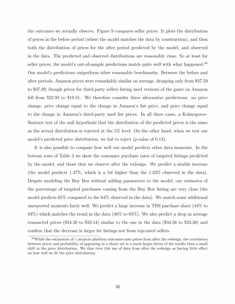
the outcomes we actually observe. Figure 9 compares seller prices. It plots the distribution

of prices in the before period (where the model matches the data by construction), and then

both the distribution of prices for the after period predicted by the model, and observed

in the data. The predicted and observed distributions are reasonably close. So at least for

seller prices, the model’s out-of-sample predictions match quite well with what happened.34

Our model’s predictions outperform other reasonable benchmarks. Between the before and

after periods, Amazon prices were remarkably similar on average, dropping only from $37.59

to $37.39, though prices for third-party sellers listing used versions of the game on Amazon

fell from $22.93 to $19.51. We therefore consider three alternative predictions: no price

change, price change equal to the change in Amazon’s list price, and price change equal

to the change in Amazon’s third-party used list prices. In all three cases, a Kolmogorov-

Smirnov test of the null hypothesis that the distribution of the predicted prices is the same

as the actual distribution is rejected at the 5% level. On the other hand, when we test our

model’s predicted price distribution, we fail to reject (p-value of 0.13).

It is also possible to compare how well our model predicts other data moments. In the

bottom rows of Table 3 we show the consumer purchase rates of targeted listings predicted

by the model, and those that we observe after the redesign. We predict a sizable increase

(the model predicts 1.47%, which is a bit higher than the 1.23% observed in the data).

Despite modeling the Buy Box without adding parameters to the model, our estimates of

the percentage of targeted purchases coming from the Buy Box listing are very close (the

model predicts 65% compared to the 64% observed in the data). We match some additional

unreported moments fairly well. We predict a large increase in TRS purchase share (44% to

83%) which matches the trend in the data (38% to 65%). We also predict a drop in average

transacted prices ($34.30 to $33.54) similar to the one in the data ($34.56 to $33.30) and

confirm that the decrease is larger for listings not from top-rated sellers.

34While the estimation of γ projects platform outcomes onto prices from after the redesign, the correlationbetween prices and probability of appearing in a choice set is a much larger driver of the results than a smallshift in the price distribution. We thus view this use of data from after the redesign as having little effecton how well we fit the price distribution.

30

6.2 Platform Design and Product Differentiation

Recall that in the simple framework of Section 2, and motivated by the experiment results

reported in Section 3, we discussed how the optimal platform design varies with product type,

especially with the degree of horizontal and vertical differentiation. The estimated model

provides a way for us to obtain a quantitative assessment of these effects by analyzing how

different platform designs perform empirically across a variety of product types. Therefore,

in this section we use the estimates more broadly (and, consequently, more out of sample)

to consider various ways of reducing search frictions across different types of products and

to identify the sources of online price markups.

We analyze these factors in Table 5. The Table compares equilibrium outcomes for

variations of the model that differ along three dimensions. Across the columns, we vary the

consideration set design. In the first and second columns, we consider using quality rank

and price rank to form consideration sets, analogous to the before and after search regimes.

In the third column, we introduce demand weights rank where listings are sampled based

on purchase probability. In the last column, we assume that all Halo Reach listings on the

platform enter each consumer’s consideration set. Across the two sets of rows in each panel,

we vary the degree of horizontal product differentiation. The “differentiation” model assumes

the estimated logit demand, in which each seller enjoys some market power. In the “limited

differentiation” model, we assume a nested logit demand structure in which the outside good

and non-targeted listings form one nest and all sellers of targeted listings are part of a second

nest. Specifically, the εij in our logit demand model (9) becomes ζ iJ + (1− σ) εij, where all

sellers of targeted listings share the same ζ iJ , whose distribution depends on σ (see Berry,

1994). The “limited differentiation” model assumes σ = 0.8, which reduces the weight on

the listing-specific error and makes the products much less differentiated than the baseline

logit “differentiation” case, which corresponds to σ = 0. Across the panels, we vary the

degree of vertical product differentiation. Panel A uses our estimated qualities for the Halo

Reach listings, a relatively homogeneous product. Panel B draws qualities from a uniform

distribution with a range 30 times larger than the estimated range for Halo Reach.35

35We choose to increase the range by a factor of 30 because this matches the degree of vertical differentiationwe estimate for a less homogeneous product, the Canon Mark II digital camera, active at the time of the

31

In the eight scenarios in Panel A, we fix the joint distribution of seller costs and quality,

and draw costs and quality for each seller on the platform (assuming 28 sellers, which is the

mean from the after period).36 For the eight scenarios in Panel B, we fix the distribution of

seller costs and draw quality from a uniform distribution over (-15,15). Sellers are assumed to

set prices knowing the assumptions about consumer search and choice behavior, but without

knowledge of the exact realization of opponents’ costs and qualities. To solve for equilibrium

prices and markups, we start from the original price distribution and update sellers’ prices

one-by-one using their first-order conditions with the counterfactual model and the new

price distribution. We continue iterating over sellers until every seller’s first-order condition

simultaneously holds.

The results can be used to understand the sources of seller margins and differential

purchase rates. Consider first the case with no search costs and limited horizontal and

vertical differentiation (top right of Panel A). In this scenario, sellers sustain positive margins

because there is some possibility that they have a strictly lower cost than all competing sellers

(as in the incomplete information Bertrand pricing model of Spulber, 1995). The median

markup is less than $0.50, and the average transaction price is $25. Purchase rates are very

high, as markups are low and users’ consideration sets include all available listings.

As we incorporate search frictions through smaller consideration sets (moving from right

to left on the top row), we see that search frictions lead to substantially increased markups

and transaction prices and decreased purchase rates. Listing horizontal differentiation, how-

ever, is an even more potent force for pricing power. For any assumption about search design,

increased seller differentiation leads to higher markups and higher prices.37 Moreover, even

with no search frictions prices are higher than in any of the limited differentiation cases.

Interestingly, once listing differentiation is present, the “price rank” search design actually

leads to more intense price competition than is present with no search frictions. The reason,

of course, is that the (limited) consideration set is selected with significant weight on price,

whereas given a choice set, consumers focus on the idiosyncratic match (the εij) as well as

redesign. Most of this product’s listings include additional accessories (an extra lens, a battery pack, etc.),consistent with a large degree of vertical differentiation.

36Across all scenarios, we also fix the consideration set size distribution to match the after period andexclude the Buy Box.

37Purchase rates are not directly comparable across the rows as they come from different demand systems.

32

price.

For a product with considerable vertical differentiation (Panel B), we reach similar con-

clusions when comparing outcomes between the no search frictions design and the designs

with limited consideration set sizes, albeit we find somewhat higher markups for this prod-

uct, supported by the increased differentiation. The main difference we see is that whereas

price rank led to a higher purchase rate for the less vertically differentiated product, qual-

ity and demand rank outperform price rank here. This insight – which is obtained from a

complete model that uses parameters estimated from actual data – is qualitatively similar to

the key insight we obtained in Section 2 from our toy example, where increasing the degree

of vertical differentiation called for a lower weighting of price in determining which product

enters the consideration set.

6.3 Discussion and Extensions

We considered a number of other permutations of the model. In one exercise, we investigated

how the platform’s choice of how many targeted versus non-targeted listings to include in

the consideration set affects pricing incentives and purchase rates. The platform may want

to have several listings of both types if some consumers are engaging in product search. The

return to replacing a targeted listing with a non-targeted listing depends on how different

the new listing is compared to the other listings already in the consideration set. In other

words, if the non-targeted listings are relatively homogeneous (λ ≈ 0), adding another will

not increase purchase rates much. The discussion also potentially relates to the importance

of obfuscation and the ability of the platform to filter less relevant listings. If the non-

targeted listings show up even for users who specify clear search terms, then better filtering

might replace some extraneous listings (e.g., iPhone covers or chargers when the search terms

clearly specify the device itself) with more relevant ones.

We first assessed the effect of replacing a single targeted listing with a non-targeted

listing. We find the purchase rate of targeted listings decreases significantly and the purchase

rate of non-targeted listings increases slightly. The effect on targeted purchase rates is

stronger because most consideration sets already include many non-targeted listings while

many include just one or two targeted listings. We also see minimal effect on seller margins.

33

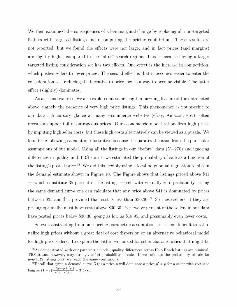
We then examined the consequences of a less marginal change by replacing all non-targeted

listings with targeted listings and recomputing the pricing equilibrium. These results are

not reported, but we found the effects were not large, and in fact prices (and margins)

are slightly higher compared to the “after” search regime. This is because having a larger

targeted listing consideration set has two effects. One effect is the increase in competition,

which pushes sellers to lower prices. The second effect is that it becomes easier to enter the

consideration set, reducing the incentive to price low as a way to become visible. The latter

effect (slightly) dominates.

As a second exercise, we also explored at some length a puzzling feature of the data noted

above, namely the presence of very high price listings. This phenomenon is not specific to

our data. A cursory glance at many e-commerce websites (eBay, Amazon, etc.) often

reveals an upper tail of outrageous prices. Our econometric model rationalizes high prices

by imputing high seller costs, but these high costs alternatively can be viewed as a puzzle. We

found the following calculation illustrative because it separates the issue from the particular

assumptions of our model. Using all the listings in our “before” data (N=270) and ignoring

differences in quality and TRS status, we estimated the probability of sale as a function of

the listing’s posted price.38 We did this flexibly using a local polynomial regression to obtain

the demand estimate shown in Figure 10. The Figure shows that listings priced above $41

— which constitute 35 percent of the listings — sell with virtually zero probability. Using

the same demand curve one can calculate that any price above $41 is dominated by prices

between $35 and $41 provided that cost is less than $30.30.39 So these sellers, if they are

pricing optimally, must have costs above $30.30. Yet twelve percent of the sellers in our data

have posted prices below $30.30, going as low as $18.95, and presumably even lower costs.

So even abstracting from our specific parametric assumptions, it seems difficult to ratio-

nalize high prices without a great deal of cost dispersion or an alternative behavioral model

for high-price sellers. To explore the latter, we looked for seller characteristics that might be

38As demonstrated with our parametric model, quality differences across Halo Reach listings are minimal.TRS status, however, may strongly affect probability of sale. If we estimate the probability of sale fornon-TRS listings only, we reach the same conclusions.

39Recall that given a demand curve D (p) a price p will dominate a price p′ > p for a seller with cost c so

long as (1− t)pD(p)−p′D(p′)D(p)−D(p′) − T > c.

34

correlated with setting high prices or equivalently having high imputed costs. The results

are in Table 6. Several measures that might be viewed as proxies for “professionalism” (of-

fering free shipping and using posted prices) are negatively correlated with high prices. But

the relationships are rather noisy, and other measures such as being top-rated, being highly

active as a seller, and being on the platform for more years are not predictive. Table 6 does

show that high-price sellers also have more Halo Reach listings, suggesting that these sellers

may be experimenting or using high-price listings to frame buyer expectations. However, we

find little support for these hypotheses: the multi-listing high-price sellers typically do not

also offer low price listings, nor do they change their prices frequently. Therefore, while we

view the high-end prices as puzzling, we lack a neat behavioral explanation, and view our

strategy of imputing high costs as a reasonable solution for our current purposes.

7 Conclusion

This paper has explored the role of platform design in online markets, emphasizing the trade-

off between reducing search frictions by matching buyers to their most desired products and

intensifying price competition among sellers. We began with a stylized theoretical framework

that illustrated the trade-off, and then used a particular episode of a platform redesign at

eBay to examine this trade-off empirically. We presented descriptive evidence pointing to

the impact of the platform design on both consumer and seller pricing behavior, and used

results from an experiment run by eBay to show that the impact of the platform design

varies quite considerably across product categories that cover more versus less homogeneous

sets of products.

The descriptive evidence also highlighted the distinction between short-run and longer-

run effects of platform design changes, and the potential for equilibrium effects that a smaller-

scale experiment may miss. In the last part of the paper, we therefore developed a complete

equilibrium model and estimated it on a narrow, yet well defined product category, where

we can quantitatively assess the platform design trade-off using counterfactual exercises.

Of course, our analysis is narrow, in the sense that we focused on specific product markets,

where products vary only in price and quality. Yet, the broader lesson that we draw from

35

our analysis regards the importance of the platform design in affecting not only consumer

behavior and reducing their search frictions, but also in affecting sellers’ decisions. Our

analysis focused on price, but similar forces would be at play for other product attributes

that can be changed in the short run, such as service quality or information disclosure. We

view our work as an initial step. With the increasing importance of internet platforms, such

as eBay, Amazon, Uber, and Airbnb, to the overall economy, we think that further studies

that would assess the efficiency of different platform designs in a variety of contexts is a

promising direction for further work.

References

Backus, Matthew, and Gregory Lewis (2016). “Dynamic Demand Estimation in AuctionMarkets.” NBER Working Paper No. 22375.

Bailey, Joseph (1998). “Intermediation and Electronic Markets: Aggregation and Pricingin Internet Commerce.” Ph.D. Thesis, Massachusetts Institute of Technology.

Baye, Michael R., and John Morgan (2001). “Information Gatekeepers on the Internet andthe Competitiveness of Homogeneous Product Markets.” American Economic Review91(3), 454-474.

Baye, Michael R., John Morgan, and Patrick Scholten (2004). “Price Dispersion in theSmall and the Large: Evidence from an Internet Price Comparison Site.” Journal ofIndustrial Economics 52(4), 463-496.

Berry, Steven T. (1994). “Estimating Discrete-Choice Models of Product Differentiation.”RAND Journal of Economics 25(2), 242-262.

Chen, Yuxin, and Song Yao (2016). “Sequential Search with Refinement: Model andApplication with Click-Stream Data.” Management Science 63(12), 4345-4365.

Damiano, Ettore, and Halo Li (2007). “Price Discrimination and Efficient Matching.”Economic Theory 30(2), 243-263.

Einav, Liran, Dan Knoepfle, Jonathan Levin and Neel Sundaresan (2014). “Sales Taxesand Internet Commerce.” American Economic Review 114(1), 1-26.

Einav, Liran, Theresa Kuchler, Jonathan Levin, and Neel Sundaresan (2015). “Assess-ing Sales Strategies in Online Markets Using Matched Listings.” American EconomicJournals: Microeconomics 7(2), 215-247

Ellison, Glenn (2005). “A Model of Add-On Pricing.” Quarterly Journal of Economics120(2), 585-637.

36

Ellison, Glenn, and Sara F. Ellison (2009). “Search, Obfuscation, and Price Elasticities onthe Internet.” Econometrica 77(2), 427-452.

Ellison, Glenn, and Sara F. Ellison (2014). “Match Quality, Search, and the Internet Marketfor Used Books.” Mimeo, MIT.

Ellison, Glenn, and Alexander Wolitzky (2012). “A Search Cost Model of Obfuscation.”RAND Journal of Economics 43(3), 417-441.

Fradkin, Andrey (2014). “Search Frictions and the Design of Online Marketplaces.” Stan-ford Working Paper.

Gabaix, Xavier, and David Laibson (2006). “Shrouded Attributes, Consumer Myopia andInformation Suppression in Competitive Markets.” Quarterly Journal of Economics121(2), 505-540.

Gomes, Renato, and Alessandro Pavan (2017). “Price Customization and Targeting inMany-to-Many Matching Markets.” Mimeo, Northwestern University.

Goeree, Michelle (2008). “Limited Information and Advertising in the U.S. Personal Com-puter Industry.” Econometrica 76(5), 1017-1074.

Hong, Han, and Matthew Shum (2006). “Using Price Distributions to Estimate SearchCosts.” RAND Journal of Economics 37(3), 257-275.

Honka, Elisabeth, Ali Hortacsu, and Maria Ana Vitorino (2014). “Advertising, ConsumerAwareness and Choice: Evidence from the U.S. Banking Industry.” Mimeo, Universityof Chicago.

Hortacsu, Ali, Babur De los Santos, and Matthijs Wildenbeest (2012). “Testing Models ofConsumer Search using Data on Web Browsing and Purchasing Behavior.” AmericanEconomic Review 102(6), 2955-2980.

Hortacsu, Ali, and Chad Syverson (2004). “Product Differentiation, Search Costs andCompetition in the Mutual Fund Industry: A Case Study of the S&P 500 Index Funds.”Quarterly Journal of Economics 119(2), 403-456.

Horton, John (2014). “Misdirected Search Effort in a Matching Market: Causes, Conse-quences and a Partial Solution.” NYU Working Paper.

Johnson, Terrence (2013). “Matching through Position Auctions.” Journal of EconomicTheory 148, 1700-1713.

Kim, Jun P., Paulo Albuquerque, and Bart J. Bronnenberg (2010). “Online Demand underLimited Consumer Search.” Marketing Science 29(6), 1001-1023.

Lewis, Gregory and Albert Wang (2013). “Who Benefits from Improved Search in PlatformMarkets?” Harvard Working Paper.

37

Malmendier, Ulrike, and Young Han Lee (2011). “The Bidder’s Curse.” American EconomicReview 101(2), 749-787.

Rochet, Jean-Charles, and Jean Tirole (2006). “Two-sided Markets: A Progress Report”RAND Journal of Economics 37(3), 645-667.

Rysman, Marc (2009). “The Economics of Two-Sided Markets.” Journal of EconomicsPerspectives 23(2), 125-143.

Smith, Michael, and Erik Brynjolfsson (2001). “Consumer Decision-Making at an InternetShopbot: Brand Still Matters.” Journal of Industrial Economics 49(4), 541-558.

Spulber, Daniel F. (1995). “Bertrand Competition when Rivals’ Costs are Unknown.”Journal of Industrial Economics 43(1), 1-11.

Stahl, Dale (1989). “Oligopolistic Pricing with Sequential Consumer Search.” AmericanEconomic Review 79(4), 700-712.

Stigler, George (1961). “The Economics of Information.” Journal of Political Economy69(3), 213-225.

Ursu, Raluca M. (2016). “The Power of Rankings: Quantifying the Effect of Rankings onOnline Consumer Search and Purchase Decisions.” Mimeo, New York University.

38

Figure1:ComparativeStaticsinPlatformChoice

Figureshowssellerprices(PanelA),sellerexanteprobabilitiesofbeingshown(PanelB),andconsumersurplusandprofits(PanelC)asafunctionoftheplatform’schoiceoftherelativeweight(β)onpricewhendeterminingwhichproducttoshowusers.

PanelA:SellerPricesasaFunctionofPlatformChoice(β)

PanelB:SellerProbabilitiesofAppearingasaFunctionofPlatformChoice(β)

PanelC:ConsumerSurplusandPlatform𝝅 asaFunctionofPlatformChoice(β)

Figure2:(ConsumerSurplus)OptimalPlatformChoice

Figureshowsβ*,theplatform’schoiceoftherelativeweighttoputonpricethatmaximizesconsumersurplus,asafunctionofconsumers’pricesensitivityindemand(PanelA),thecostofthehigher-qualityproduct(PanelB),thequalitydifferencebetweentheproducts(PanelC),andtheplatform’snoiseinobservingquality(PanelD).Parametersarefixedatα=0.5,q=1,c=0.5q,andσ=1unlesstheyaretheparameterbeingvariedforthecomparativestatic.Theplatformcharges0.3pertransactionandkeeps0.1ofthetransactedprice.

PanelA:β*asaFunctionofα PanelB:β*asaFunctionofc

PanelC:β*asaFunctionofq PanelD:β*asaFunctionofσ

Figure3:Differentapproachestoplatformdesign

Figureshowssearchresultsfollowingaqueryfor“playstation 3”onCraigslist(top),GoogleShopping(middle),andAmazon(bottom).

Craigslist

GoogleSho

pping

Amazon

Figure4:eBay’splatformre-design

Figure shows the change in eBay’s presentation of search results. The top panel shows eBay’s Best Match results. Thebottom panel shows a product page, with listings ordered by sales format and price.

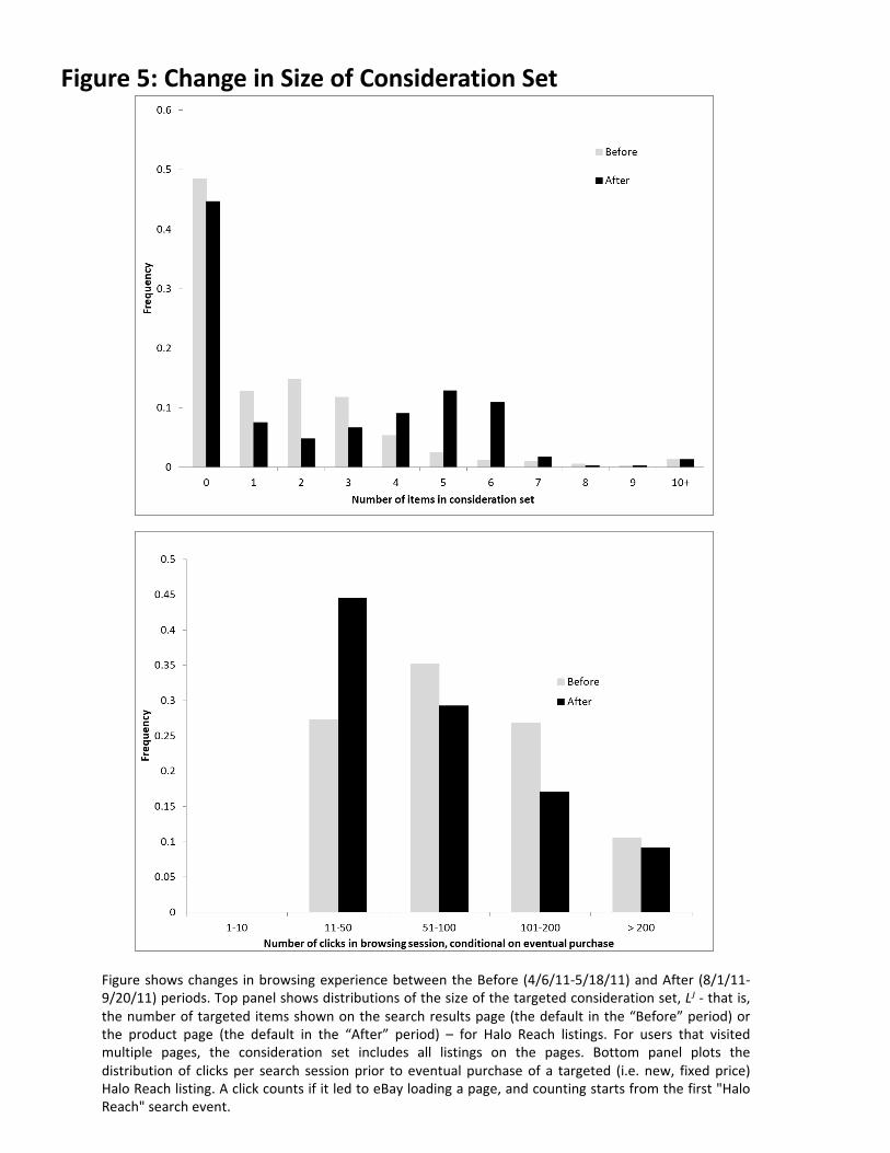
Figure5:ChangeinSizeofConsiderationSet

Figure shows changes in browsing experience between the Before (4/6/11-5/18/11) and After (8/1/11-9/20/11) periods. Top panel shows distributions of the size of the targeted consideration set, LJ - that is,the number of targeted items shown on the search results page (the default in the “Before” period) orthe product page (the default in the “After” period) – for Halo Reach listings. For users that visitedmultiple pages, the consideration set includes all listings on the pages. Bottom panel plots thedistribution of clicks per search session prior to eventual purchase of a targeted (i.e. new, fixed price)Halo Reach listing. A click counts if it led to eBay loading a page, and counting starts from the first "HaloReach" search event.

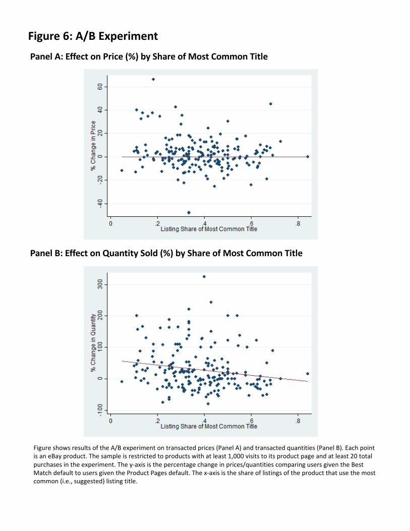
Figure6:A/BExperiment

FigureshowsresultsoftheA/Bexperimentontransactedprices(PanelA)andtransactedquantities(PanelB).EachpointisaneBayproduct.Thesampleisrestrictedtoproductswithatleast1,000visitstoitsproductpageandatleast20totalpurchasesintheexperiment.They-axisisthepercentagechangeinprices/quantitiescomparingusersgiventheBestMatchdefaulttousersgiventheProductPagesdefault.Thex-axisistheshareoflistingsoftheproductthatusethemostcommon(i.e.,suggested)listingtitle.

PanelA:EffectonPrice(%)byShareofMostCommonTitle

PanelB:EffectonQuantitySold(%)byShareofMostCommonTitle

Figure7:ImpliedCostDistribution

Figure shows the distribution of seller costs imputed from the observed prices and the sellers’ first ordercondition. This cost distribution is assumed to remain the same after the platform re-design, and is heldfixed in the counterfactual exercises. The dashed black line shows the cost distribution of TRS sellers; thesolid black line is non-TRS sellers. The optimal mark-ups associated with each level of cost, given ourdemand estimates, are presented by the gray lines for TRS and non-TRS.

Figure8:EstimatedDemandCurves

Figure plots demand curves based on our model estimates. The x-axis is the per-search probability of beingtransacted, which is the probability of appearing in the consideration set multiplied by the probability ofbeing transacted conditional on being in the consideration set.

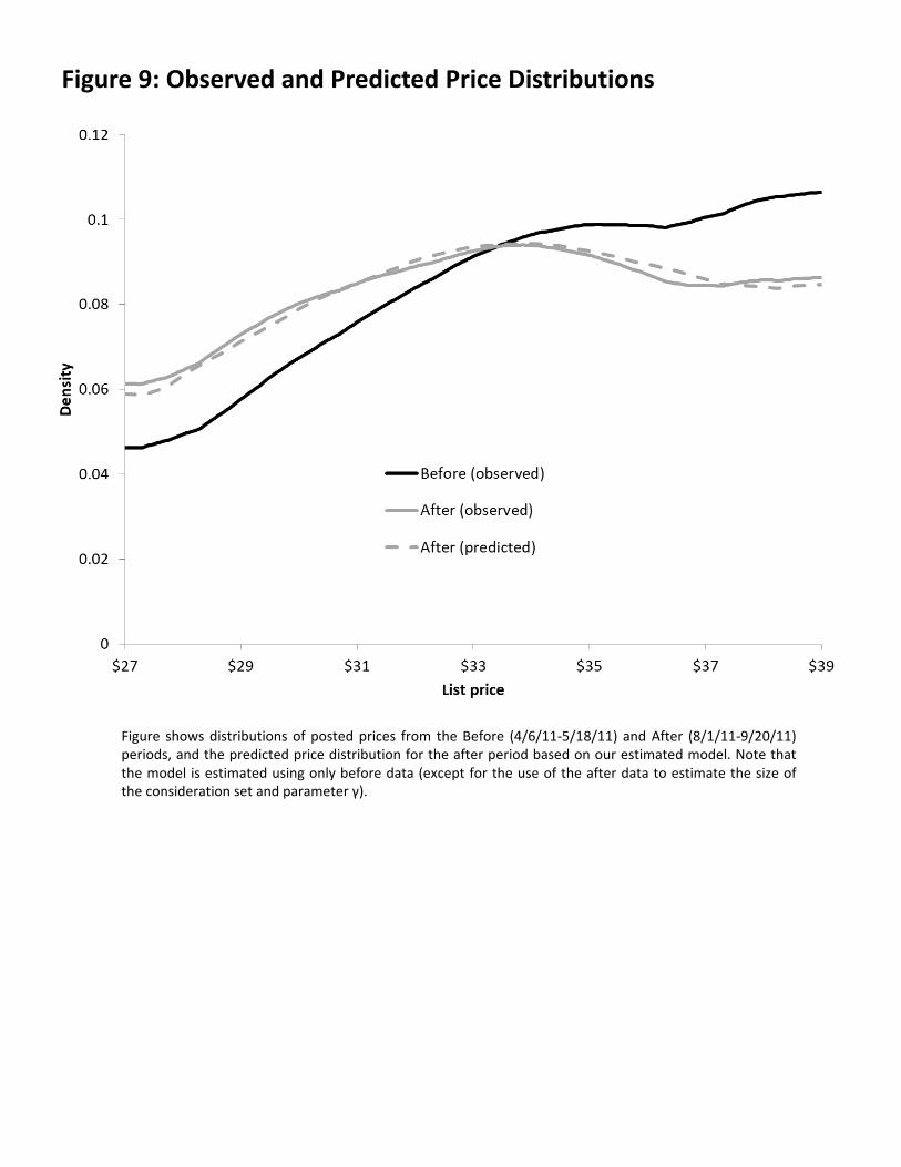
Figure9:ObservedandPredictedPriceDistributions

Figure shows distributions of posted prices from the Before (4/6/11-5/18/11) and After (8/1/11-9/20/11)periods, and the predicted price distribution for the after period based on our estimated model. Note thatthe model is estimated using only before data (except for the use of the after data to estimate the size ofthe consideration set and parameter γ).

Figure10:Non-ParametricPlotofListingDemand

Figure shows the probability of sale for listings in the before period, estimated using a local polynomialregression plotted against listing price. The sample size is N=270 listings.

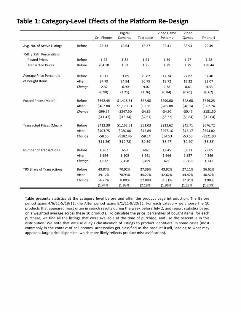
Table1:Category-LevelEffectsofthePlatformRe-Design

Table presents statistics at the category level before and after the product page introduction. The Beforeperiod spans 4/6/11-5/18/11; the After period spans 8/1/11-9/20/11. For each category we choose the 10products that appeared most often in search results during the week before July 2, and report statistics basedon a weighted average across these 10 products. To calculate the price percentiles of bought items: for eachpurchase, we find all the listings that were available at the time of purchase, and use the percentile in thisdistribution. We note that we use eBay’s classification of listings to product identifiers. In some cases (mostcommonly in the context of cell phones, accessories get classified as the product itself, leading to what mayappear as large price dispersion, which more likely reflects product misclassification).

CellPhones

Digital

Cameras Textbooks

VideoGame

Systems

Video

Games iPhone4

Avg.No.ofActiveListings Before

75th/25thPercentileof

PostedPrices Before

TransactedPrices Before

AveragePricePercentile Before

23.33 40.64 16.27 35.41 38.93 29.49

1.22 1.32 1.61 1.39 1.47 1.28

204.10 1.31 1.25 1.29 1.29 138.44

40.11 31.85 29.82 17.34 27.82 37.40

ofBoughtItems After

Change37.79 24.94 20.75 19.72 19.22 33.07

-2.32 -6.90 -9.07 2.38 -8.61 -4.33

(0.98) (1.21) (1.76) (0.84) (0.61) (0.62)

PostedPrices(Mean) Before $562.45 $1,418.31 $67.98 $290.00 $48.60 $749.25

After

Change

TransactedPrices(Mean) Before

$462.88 $1,170.81 $63.11 $285.08 $48.14 $567.74

-$99.57 -$247.50 -$4.86 -$4.92 -$0.45 -$181.50

($11.47) ($13.14) ($2.61) ($5.32) ($0.84) ($12.04)

$412.30 $1,162.51 $51.03 $222.62 $45.71 $676.72

After

Change

NumberofTransactions Before

$403.75 $980.06 $42.89 $257.16 $42.17 $554.82

-$8.55 -$182.46 -$8.14 $34.53 -$3.53 -$121.90

($11.26) ($10.78) ($0.59) ($3.47) ($0.40) ($6.83)

1,762 650 482 1,045 3,873 2,605

After

Change

TRSShareofTransactions Before

3,594 3,108 3,941 1,666 2,537 4,346

1,832 2,458 3,459 621 -1,336 1,741

43.87% 70.92% 27.39% 43.92% 27.11% 36.62%

After

Change39.12% 78.93% 45.27% 42.62% 44.42% 40.52%

-4.75% 8.00% 17.88% -1.31% 17.31% 3.90%

(1.44%) (1.93%) (2.18%) (1.96%) (1.22%) (1.20%)

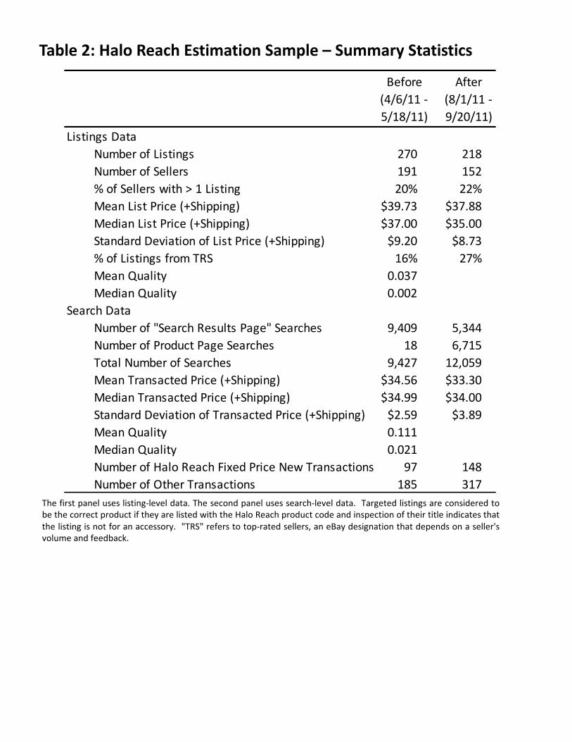
Table2:HaloReachEstimationSample– SummaryStatistics

The first panel uses listing-level data. The second panel uses search-level data. Targeted listings are considered tobe the correct product if they are listed with the Halo Reach product code and inspection of their title indicates thatthe listing is not for an accessory. "TRS" refers to top-rated sellers, an eBay designation that depends on a seller'svolume and feedback.

Before(4/6/11-5/18/11)

After(8/1/11-9/20/11)

ListingsDataNumberofListings 270 218NumberofSellers 191 152%ofSellerswith>1Listing 20% 22%MeanListPrice(+Shipping) $39.73 $37.88MedianListPrice(+Shipping) $37.00 $35.00StandardDeviationofListPrice(+Shipping) $9.20 $8.73%ofListingsfromTRS 16% 27%MeanQuality 0.037MedianQuality 0.002

SearchDataNumberof"SearchResultsPage"Searches 9,409 5,344NumberofProductPageSearches 18 6,715TotalNumberofSearches 9,427 12,059MeanTransactedPrice(+Shipping) $34.56 $33.30MedianTransactedPrice(+Shipping) $34.99 $34.00StandardDeviationofTransactedPrice(+Shipping) $2.59 $3.89MeanQuality 0.111MedianQuality 0.021NumberofHaloReachFixedPriceNewTransactions 97 148NumberofOtherTransactions 185 317

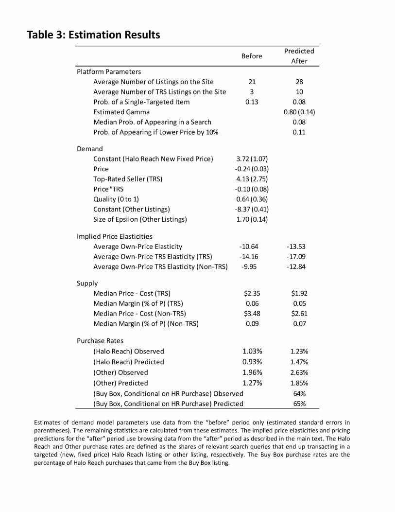
Table3:EstimationResults

Estimates of demand model parameters use data from the “before” period only (estimated standard errors inparentheses). The remaining statistics are calculated from these estimates. The implied price elasticities and pricingpredictions for the “after” period use browsing data from the “after” period as described in the main text. The HaloReach and Other purchase rates are defined as the shares of relevant search queries that end up transacting in atargeted (new, fixed price) Halo Reach listing or other listing, respectively. The Buy Box purchase rates are thepercentage of Halo Reach purchases that came from the Buy Box listing.

BeforePredictedAfter

PlatformParametersAverageNumberofListingsontheSite 21 28AverageNumberofTRSListingsontheSite 3 10Prob.ofaSingle-TargetedItem 0.13 0.08EstimatedGamma 0.80(0.14)MedianProb.ofAppearinginaSearch 0.08Prob.ofAppearingifLowerPriceby10% 0.11

DemandConstant(HaloReachNewFixedPrice) 3.72(1.07)Price -0.24(0.03)Top-RatedSeller(TRS) 4.13(2.75)Price*TRS -0.10(0.08)Quality(0to1) 0.64(0.36)Constant(OtherListings) -8.37(0.41)SizeofEpsilon(OtherListings) 1.70(0.14)

ImpliedPriceElasticitiesAverageOwn-PriceElasticity -10.64 -13.53AverageOwn-PriceTRSElasticity(TRS) -14.16 -17.09AverageOwn-PriceTRSElasticity(Non-TRS) -9.95 -12.84

SupplyMedianPrice-Cost(TRS) $2.35 $1.92MedianMargin(%ofP)(TRS) 0.06 0.05MedianPrice-Cost(Non-TRS) $3.48 $2.61MedianMargin(%ofP)(Non-TRS) 0.09 0.07

PurchaseRates(HaloReach)Observed 1.03% 1.23%(HaloReach)Predicted 0.93% 1.47%(Other)Observed 1.96% 2.63%(Other)Predicted 1.27% 1.85%(BuyBox,ConditionalonHRPurchase)Observed 64%(BuyBox,ConditionalonHRPurchase)Predicted 65%

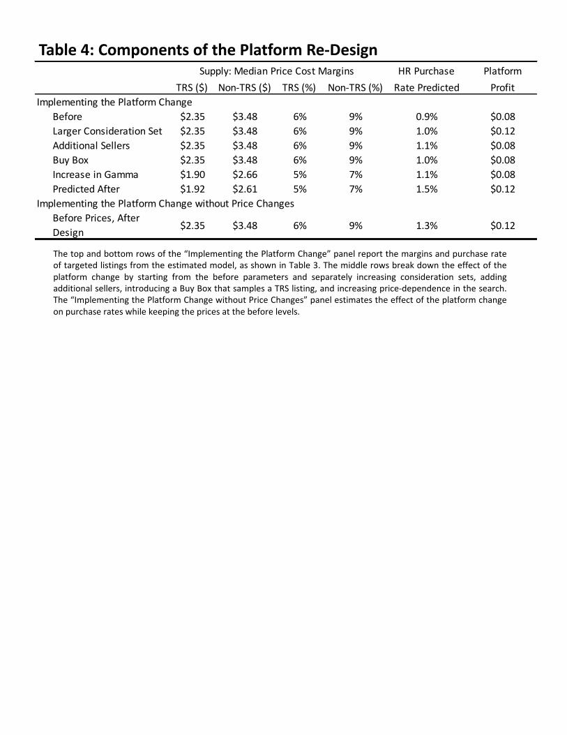
Table4:ComponentsofthePlatformRe-Design

The top and bottom rows of the “Implementing the Platform Change” panel report the margins and purchase rateof targeted listings from the estimated model, as shown in Table 3. The middle rows break down the effect of theplatform change by starting from the before parameters and separately increasing consideration sets, addingadditional sellers, introducing a Buy Box that samples a TRS listing, and increasing price-dependence in the search.The “Implementing the Platform Change without Price Changes” panel estimates the effect of the platform changeon purchase rates while keeping the prices at the before levels.

Supply:MedianPriceCostMargins HRPurchase PlatformTRS($) Non-TRS($) TRS(%) Non-TRS(%) RatePredicted Profit

ImplementingthePlatformChangeBefore $2.35 $3.48 6% 9% 0.9% $0.08LargerConsiderationSet $2.35 $3.48 6% 9% 1.0% $0.12AdditionalSellers $2.35 $3.48 6% 9% 1.1% $0.08BuyBox $2.35 $3.48 6% 9% 1.0% $0.08IncreaseinGamma $1.90 $2.66 5% 7% 1.1% $0.08PredictedAfter $1.92 $2.61 5% 7% 1.5% $0.12

ImplementingthePlatformChangewithoutPriceChangesBeforePrices,AfterDesign $2.35 $3.48 6% 9% 1.3% $0.12

Table5:TheImpactofSearchFrictions

Panel A uses the estimated quality distribution from the Halo Reach product used in estimation. Panel Bconsiders a hypothetical product with 30 times the dispersion in quality of Halo Reach. The labels "SellerDifferentiation" and “Limited Seller Differentiation" refer to whether we include a seller-specific logit errorfor targeted listings. The version with differentiation keeps the error, while the “Limited Differentiation”specification assumes a nested logit model in which all “targeted listings” are in the same nest and thenested logit σ parameter is set to 0.8. Each column refers to a different platform design: Quality Rank (the“Before” regime), Price Rank (the “After” regime), a counterfactual regime with Demand Weights Rank, anda counterfactual regime in which consumers are shown the entire set of targeted listings available on theplatform.

PanelA:UsingEstimatedQuality

PanelB:UsingQualitywith30xtheDispersionofEstimatedQuality

UsingEstimatedQuality

QualityRank("Before")

PriceRank("After")

DemandWeightsRank

NoFrictions(allitemsvisible)

MedianMarkup $1.95 $1.71 $1.71 $0.45MeanTransactedPrice $33.37 $32.03 $32.04 $24.61PurchaseRate(HR) 1.1% 1.4% 1.4% 2.6%PurchaseRate(Other) 2.4% 2.2% 2.2% 2.1%PlatformProfit $0.12 $0.12 $0.12 $0.14

MedianMarkup $3.57 $2.58 $2.59 $3.46MeanTransactedPrice $34.70 $33.02 $33.05 $33.56PurchaseRate(HR) 1.2% 1.4% 1.4% 2.2%PurchaseRate(Other) 2.1% 2.0% 2.0% 1.7%PlatformProfit $0.12 $0.12 $0.12 $0.12

LimitedSellerDifferentiation

SellerDifferentiation

SearchDesign

ScalingupQualityDifferentiation

QualityRank("Before")

PriceRank("After")

DemandWeightsRank

NoFrictions(allitemsvisible)

MedianMarkup $2.90 $2.24 $2.85 $0.90MeanTransactedPrice $37.84 $36.33 $37.79 $40.61PurchaseRate(HR) 2.7% 2.6% 2.7% 9.8%PurchaseRate(Other) 2.3% 2.5% 2.2% 1.6%PlatformProfit $0.19 $0.19 $0.19 $0.48

MedianMarkup $3.46 $2.59 $3.45 $3.46MeanTransactedPrice $38.24 $36.55 $38.20 $40.26PurchaseRate(HR) 2.7% 2.6% 2.8% 7.0%PurchaseRate(Other) 2.2% 2.4% 2.1% 1.6%PlatformProfit $0.19 $0.18 $0.19 $0.36

SearchDesign

LimitedSellerDifferentiation

SellerDifferentiation

Table6:ExplanationofHighSellerCosts

Table shows results from univariate regressions where each observation is a seller in the beforeperiod (N=191) and the dependent variable is an indicator equal to 1 if the seller’s imputed cost fromthe model is above $40 for at least one of his Halo Reach listings. The covariates pertaining tocharacteristics of seller listings are generated using all listings by the seller over 2009-2011.

Top-RatedSellerDummy -0.024 (0.080)YearsoneBay(Truncatedat5) 0.006 (0.036)%ListingsFixedPrice -0.176 (0.070)%ListingsFreeShipping -0.152 (0.071)

Log(TotalHaloReachListings) 0.040 (0.020)Log(TotalVideogameListings) 0.008 (0.009)Log(TotaleBayListings) 0.010 (0.009)Log(QAvailableinAllListings) 0.012 (0.008)Log(QSoldinAllListings) 0.000 (0.010)Log(NumCategoriesListingin) 0.002 (0.022)

AnyHaloReachPriceChange 0.080 (0.070)

UnivariateRegressionsDepVar:Dummyfor

Seller'sMaxCost>$40