Embed Size (px)
Citation preview
Consumer Demand Modeling During COVID-19Pandemic
Shaz HodaEmerging Technology
PwCNew York, USA
Amitoj SinghEmerging Technology
PwCMumbai, India
Anand RaoEmerging Technology
PwCBoston, USA
Remzi UralConsumer Markets
PwCChicago, USA
Nicholas HodsonConsumer Markets
PwCUtah, USA
Abstract—The current pandemic has introduced substantialuncertainty to traditional methods for demand planning. Theseuncertainties stem from the disease progression, governmentinterventions, economy and consumer behavior. While most ofthe emerging literature on the pandemic has focused on diseaseprogression, a few have focused on consequent regulations andtheir impact on individual behavior. The contributions of thispaper include a quantitative behavior model of fear of COVID-19, impact of government interventions on consumer behavior,and impact of consumer behavior on consumer choice and hencedemand for goods. It brings together multiple models for diseaseprogression, consumer behavior and demand estimation– thusbridging the gap between disease progression and consumerdemand. We use panel regression to understand the drivers ofdemand during the pandemic and Bayesian inference to simplifythe regulation landscape that can help build scenarios for resilientdemand planning. We illustrate this resilient demand planningmodel using a specific example of gas retailing. We find thatdemand is sensitive to fear of COVID-19 – as the number ofCOVID-19 cases increase over the previous week, the demandfor gas decreases - though this dissipates over time. Further, gov-ernment regulations restrict access to different services, therebyreducing mobility, which in itself reduces demand.
Index Terms—forecasting, scenario modeling, demand forecast-ing, panel regression, segmentation, Bayesian inference
I. INTRODUCTION
Understanding demand and its drivers in the pre-pandemicera was about understanding underlying demographic charac-teristics of the customers and short-run price and promotiondecisions of the supplier [1]. Given that consumer preferencesand characteristics change slowly over time and price andpromotions have temporary effects on demand, it is simple touse machine learning techniques to understand the drivers ofdemand and to make short (few weeks), medium (few months)and even in some cases, long run (few years) predictions [2].These stable relationships, however, have all broken downduring the pandemic. Though traditional factors still determinedemand to an extent, new drivers become more importantas individuals make decisions that change rapidly with thechanging environment. This makes demand planning andconsequently, planning for production and distribution difficultin consumer markets. Given the lack of certainty in demand, itis important to 1) understand the right demand drivers and 2)to be able to model them correctly so as to get to an accurateunderstanding and forecast demand under different potential
scenarios. Further, these demand forecasts/scenarios need tobe available not just at a national level, but also at local levels.
A substantial body of research on the pandemic has focusedon disease progression [3][4][5][6] with a few looking at theconsequent regulations and their impact on individual behavior[7][8][9]. On demand forecasting during the pandemic, re-searchers have demonstrated that reopening of businesses andthe return to normalcy will depend not only on regulations butalso on the actions of related businesses, and customers andsuppliers as well [10]. Researchers have also identified driversof household consumption behavior during the pandemic rang-ing from demographic characteristics, political orientation,geographic location and to a lesser extent, income [11]. Ourpaper combines these strands of work by examining theinteraction of these common demand drivers with regulationsand testing these drivers along with others for their significancein predicting demand fluctuations.
The objective of our paper is to consolidate various factorsthat are impacting consumer demand during the pandemic, aswell as to provide an empirical model to estimate demandat local level. We use a demand modeling example of a gasretail company for this paper. For modeling purposes we usegas demand data for 2019 and 2020 (from a gas retaileroperating in USA), the data is available at store level for 1000+stores in 30+ states in the US. We augment this data withmultiple rich data sources and run different models LSTM,SARIMAX and panel regression to arrive at variables that cansignificantly explain the gas demand in 2020 as percentage ofgas demand in 2019 for the same week. We finally choosepanel regression for two main reasons - 1) lack of data toproperly tune other models for over-fitting and 2) for thehigh degree of interpretability that panel regression allows.We then simplify the regulation landscape and determine howthe simplified regulation landscape influences these driversto develop scenarios for planning. This approach towardsdemand modeling for gas, with slight modifications, can beextrapolated to modeling demand for other consumer goodssuch as restaurants, apparel, groceries etc.
II. DATA
As discussed in the previous section there are multiplefactors that influence demand and the objective of this paper is
978-1-7281-6215-7/20/$31.00 ©2020 IEEE
arX
iv:2
105.
0103
6v1
[cs
.AI]
3 M
ay 2
021
to create a well-founded framework for determining demanddrivers during the pandemic and testing the same empirically.The drivers are then interplayed with regulations to developplanning scenarios.
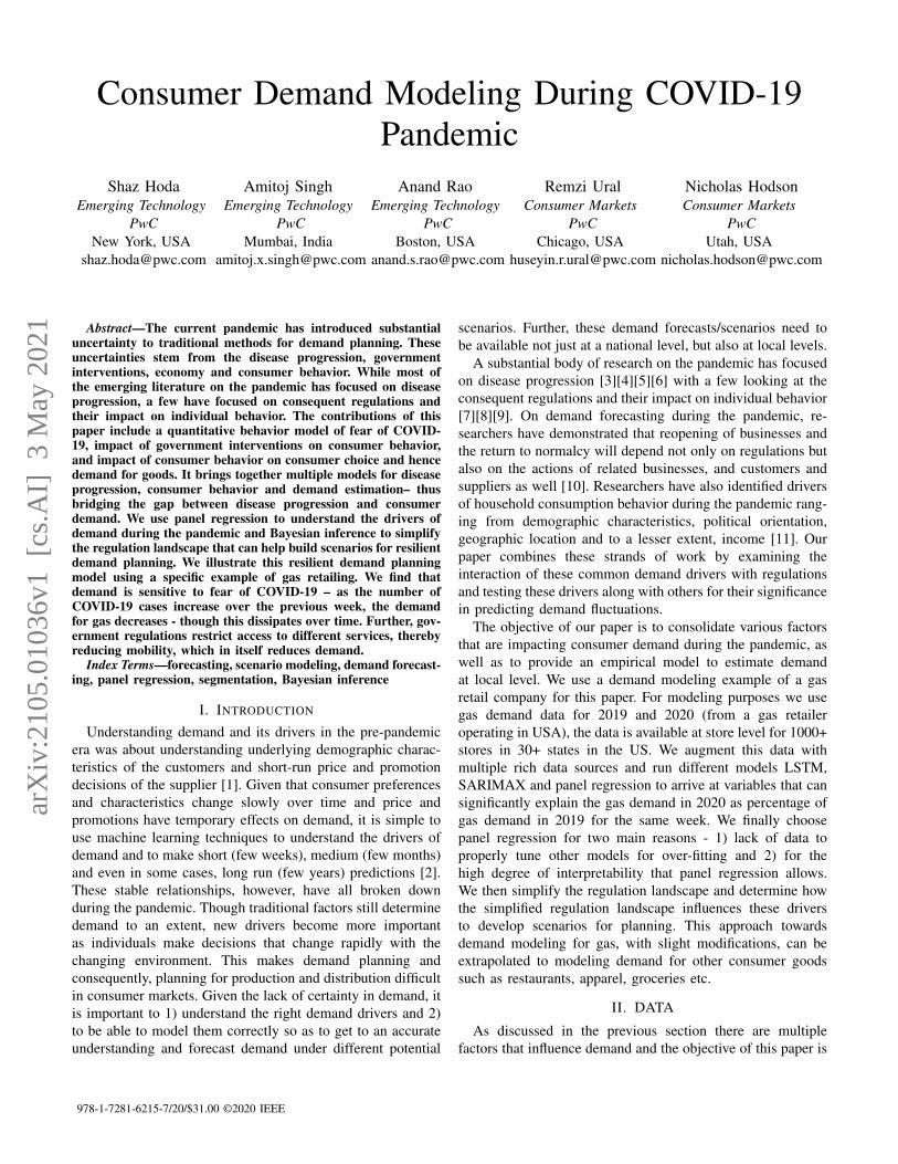
Figure 1 is a systems representation of how uncertaintiesfrom the disease, government intervention, economy and cus-tomer behavior are all intricately linked and cause uncertaintyin supply and demand.
Fig. 1: Systems view of the pandemic and its impact onsociety.
Source: Authors’ depiction.
We begin with laying multiple hypotheses for drivers ofdemand. Through interviews conducted with various expertsin the consumer goods industry, a survey of literature andworking with varied companies, we break down the potentialdemand drivers into following categories of data that wecollect:
A. Macro Indicators
COVID-19 has led to socio-economic effects and behavioralchanges because of different policies and regulations adoptedby governments across the globe, and because of changes inmacro-economic environment of countries – most countriesreporting sharp contraction of GDPs for 3rd quarter of FY20[10]. These effects have impacted countries and regions, witheach regime adopting its own set of regulations . While dipsin infections have shown signs of recoveries in countries likeJapan and South Korea, a second wave of pandemic andstricter controls have been anticipated in most US states andEU. There has also been a significant variability in the macro-economic response of governments - US and EU countriesresponded by providing stimulus packages and thereby boost-ing demand, while developing countries such as India, Mexico,are more fiscally constrained [11]. These effects are essentialfor understanding the state-specific impacts of the pandemicon various industries within the USA and therefore, we haveincluded the following set of key variables for the purpose ofour analysis.
• GDP growth rate at national/state level for USA from IHSMarkit - GDP growth rate is a good indicator of overalldemand/income in the economy and can potentially in-form demand for individual products
• Unemployment rate at the state level for USA from IHSMarkit - Unemployment rate directly impacts consumerability to spend. The job losses have been skewed towardscertain sectors – for example, leisure and hospitality beingone of the worst-hit sectors. The impact of unemploymentwas mitigated by the stimulus-package in June, but as itseffects wear down, the demand for retail-products alsofalls significantly [12]. These disparities in job lossesaffect demand for different goods across different states.
• Personal Consumption Expenditures at state level forUSA from IHS Markit - Less disposable income or pref-erence to spend during the uncertain time of a pandemiccan adversely impact demand [13].
• COVID-19 Spread from Suspected, Infected, Recovered(SIR) models at USA state level developed by the au-thors – The SIR model is an epidemiological modelindicating the number of infections in a population, basedon infection-rates, susceptibility rates and recovery-rates.The spread of infections captures the fear of differentindividuals in an environment interacting with differentfactors like strictness of lockdowns, going out and mo-bility norms [14].
• Regulations data at state level for USA from Multistate -Regulations such as closure of bars, restaurants and storesdirectly affect consumer choice and hence demand forcertain types of products.
B. Micro Indicators
It is also important to look at how pandemic has specificallychanged consumer habits at an individual level. While themacro effects help explain region specific variations, individ-ual response to the pandemic, has also impacted aggregateconsumer demand– mainly via less mobility and more timespent at home. With most white-collared offices moving to-wards a work from home based approach [12] – significantreduction in mobility levels have been noted across the world.Moreover, reduction in mobility has also, at occasions, resultedin a preference for home-consumable products proved overoutside-consumption. For example: we noted that there hasbeen a noticeable increase in sales of salad dressing forconsumer goods companies – a ’substitution effect’ for visits torestaurants. To capture the mobility related effects, we lookedat various indicators of mobility for individuals collectedthrough Google Mobility and PlaceIQ. Different indicators ofmobility at state/local level can indicate change in behavior ofconsumer and shifting preferences
• Work from Home Index (WFHI) at county level – Wemeasure work-from-home as a percentage change in timespent at work places compared to the median value in the5-week period: Jan 3 – Feb 6, 2020. A higher work fromhome results in fewer trips and less urban mobility [12].We source WFHI data from Google mobility at a countylevel and map the WFHI of the county in which the storeis located against each store.
• Stay at Home Index (SAHI) at county level – Similarto WFHI, SAHI captures the percentage change in time
spent at home as compared to the median value in the5-week period: Jan 3 – Feb 6, 2020. We source SAHIdata from Google mobility at a county level and map theSAHI of the county in which the store is located againsteach store
• Visits to grocery stores at county level - Higher visits togrocery stores could be an indicator of consumer prefer-ences shifting towards home cooked meals as comparedto restaurants [15][16]. In our case, for gas retail, visits togrocery stores were particularly important since the gasstations were generally attached to grocery store chains.We source visits to grocery stores data from PlaceIQ ata county level and map the grocery visits of the countyin which the store is located against each store
Consumer habits and surveys at county levels - Different in-dicators of consumer behavior captured through representativesurveys
• Comfort in going out during pandemic• Activities that consumers miss the most
C. Company Data
We were provided with gas volumes for a company thatowns gas-stations across various states in the US. The storeswere distributed across 30+ US states, significantly present inrural sites (60% of total stores). The data was at a weeklylevel for the 2 years – 2019 and 2020, and we modelled thegas-volumes sold in 2020 as a percentage of sales in 2019levels for the same period. This was done in order to removethe seasonality-effects, to understand demand fall relative tonormal-levels and finally to forecast a recovery compared to2019 levels. Overall the master data for analysis was createdat store week level, with dependent variable as 2020 sales asa proportion of 2019 sales for the same week. For each storethe drivers, discussed in previous two sections, were mapped- based on their granularity- to either the county or the statein which the store belonged.
III. METHODOLOGY
With the above data, we wanted to explain and projectdemand for gas. We followed a three step process to theproblem:
A. Testing hypotheses and choosing best fit model
We used the above set of explanatory variables to understandthe impact of the current pandemic on gas-sales. For ouranalysis, we considered all the macro and micro indicators.However, we leave out regulations from hypotheses testing ofinitial drivers because all other variables are impacted by state,local and national regulations – we come back to regulationsas an overarching variable, once the initial driver model is laidout. For example, the macro variable unemployment is causeddue to states mandating closure of certain businesses. Similarlythe micro variable stay at home is impacted by closure ofbusiness and firms responding to government regulations andguidelines.
For testing our hypothesis we tried three different machinelearning methods:
• Deep Learning based LSTM method - Long short-termmemory (LSTM) is an artificial recurrent neural network(RNN) architecture [17]. LSTM networks are well-suitedto classifying, processing and making predictions basedon time series data.
• SARIMAX models - Seasonal Auto Regressive Inte-grated Moving Averages with Exogenous regressors. Sea-sonal ARIMAX, is an extension of ARIMA that explic-itly supports univariate time series data with a seasonalcomponent and exogenous regressors. It adds three newhyperparameters to specify the autoregression (AR), dif-ferencing (I) and moving average (MA) for the seasonalcomponent of the series, as well as additional parametersfor the period of the seasonality and exogenous variables.
• Panel regression model with time series adjustments- Panel regression tries to overcome the limitations of orordinary least-squares regressions (OLS) by introducingfixed and random effects variables across individuals(states in our case) and time. As we show in subsequentsections, this model gives us the best fit and interpretabil-ity of the model.
B. Overlaying impact of regulations
Once a best fit model is constructed – based on error ratesand explainability - we need to develop a model that caninform scenarios on the underlying drivers. For instance, weare most interested in understanding how these variables areinterrelated and are determined by overarching factors. Fordetermining the movement of these variables and possible sce-narios, we introduce the variable of government regulations.With restrictions passed by governments around mobility ofindividuals and functioning of businesses, especially in theUSA, different macro and micro indicators that we considerare impacted.
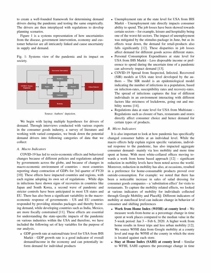
Figure 2 shows how different micro indicators (sourcedfrom Google mobility data) behaved as different regulationsand announcements were made in Texas, as an example.
Given the importance of regulations in determining bothmacro and micro indicators we procure regulations data inthe form of severity of closure/opening of certain businesses,defined with an openness at three different levels. Table 2(presented in Appendix) shows different types of regulationswe capture and how they are classified as Level 1 (mostlyopen) - Level 4 (mostly closed) based on severity.
C. Building scenarios
After the models are built and the regulation landscapeis set, we use regulations as overarching variables for de-termining the scenarios and estimating the demand giventhe regulation level. Through our approach, detailed in asubsequent section, the models learn the dependence betweenthe regulation and our set of micro and macro indicators,taking into account both time-based and location-based effects.Once this is achieved, all the end user needs to do is to specify
Fig. 2: Different Regulations and Announcements in one ofthe US States and associated mobility
Source: Author’s analysis based on Google Mobility and PlaceIQ data
restrictions for a given time period and location to generateforecasts for the underlying product. This gives the end userthe flexibility to plan for both easing and re-imposition ofrestrictions and hence adopt a resilient strategy for the future.The scenario modeling approach involves the following steps:1) the user chooses expected regulation levels in differentUS states across time or chooses from pre-built regulatoryscenarios (gradual easing/winter lockdown) 2) based on thechosen regulations, we use the mathematical model to arriveat forecasts of drivers 3) we use the forecasted drivers tounderstand how they can impact demand in the future andcreate an estimate.
IV. FINDINGS AND RESULTS
We present in this section of the paper, anonymized resultsfor retail gas demand projections to understand the demand forcommonly consumed consumer goods across multiple storesin different states. As discussed, in the previous section wefollowed the three step approach to understand demand and tobuild scenarios on it:
A. Testing hypotheses and choosing best fit model
• LSTM - though promising in terms of model error rates,the models generally have a tendency to quickly overfitunless regularized properly, which can be a tedious task.These models are also black box models which tend tooverweight variables that can have a high degree of corre-lation with the target variable, even though a theoreticalfoundation may be missing. Hence, we avoid pursuingthis method further for demand scenario modeling. Weleave LSTM models as a topic to explore further as moredata on the pandemic becomes available.
• SARIMAX model - This model gives promising results,however, requires careful tuning of seasonality for whicha long history of data is required to come up with a rea-sonable estimation of seasonality and other components.The company had about one and a half years’ worth ofdata, including the pandemic period. This made it difficult
to estimate reasonable models using SARIMAX and haveenough data points to validate the model.
• Panel regression analysis - We finally went ahead withthis approach to estimate demand. These models offerenough flexibility to fine tune variables and to get param-eter estimates to help ensure that model coefficients areas expected. The panel time series model helps us captureboth location-specific and time-specific attributes, whichthe other models LSTM (lack of interpretability) andSARIMAX (lack of location attributes) fail to capture.As we were dealing with significant heterogeneity bothin terms of locations -1000+ stores spread across 30+states – and in terms of time based effects in COVID-19responses and infection – for example: states differed bydate of first cases reported and periods of second-wave– controlling for such unobserved factors was important,which a panel model enabled us do in a simpler way.In this section we investigate the results of our panelregression model further. We also overcome the issueof estimation of seasonality by constructing our targetvariable as change in demand over previous year. Thefinal functional form of our panel regression is as follows:
Yisct = αi + β1Xist + β2Vic + β3Zict + εisct (1)
Where the dependent variable Yisct is the ratio of gasdemand in 2020 to 2019 in store i, state s, county c, and timeperiod t. The explanatory variables such as unemployment areeither at state Xist or such as SAHI at the county (Vic) level.
As mentioned above, as a precursor to the panel model,we segmented the stores to cluster similar stores together.Taking fall in demand during the first 16 weeks of thepandemic as our target variable, we ran a decision tree onusing characteristics underlying the store. These characteristicsincluded multiple demographic information pertaining to theneighborhood in which the stores were located - e.g. averageage, household income, ethnicity, rural/urbanness and othersuch characteristics that are available from the US census.The decision tree model segmented the stores into 3 distinctsegments (the client was present primarily in rural and semi-urban markets and not in major cities):
1) Primarily rural stores with low population density -These stores saw the least fall in demand.
2) Primarily urban stores with medium population densitywith low education prevalence
3) Primarily urban stores with medium population densitywith high education prevalence - These stores saw ahuge fall in demand, presumably due to higher workfrom home of urban educated
For each of these segments we created a regression model tounderstand how different macro and micro economic factorsdrive demand. There were four factors that came out to besignificant at 5% confidence levels across all three segments:
• Fear of COVID-19: COVID-19 infection rate dampedexponentially with elapsed time. This variable capturesthe fear of individuals to freely pursue activities that
influence demand of a product. For example, demandfor fashionable clothing is low, since people during thefirst few weeks of pandemic largely stayed at homedue to the lack of awareness and riskiness of the virus.This fear, however, dissipated over time. We observed inour data that demand for products goes up over time,even when all else remains the same. That is, if a statewas stuck at a certain level of regulation, it would stillsee an increase in gas demand overtime as people gotused to the new normal and found alternate activities.We experimented with multiple functional forms of thisvariable - linear dampening, log case dampened linearlyand exponential damping. The model with exponentialdampening of fear gave the best results in terms ofmeaningful and significant coefficients along with high r-squared. Through our panel approach we test for differentdampening effects across different states, however, wedon’t observe any significant differences across states inthe dampening rate or function. The final fear of COVID-19 variable for each week (t) and each state (i) took thefollowing form:
logCOV ID19infectionsist
e0.12∗t
The factor of 0.12 for dampening effect came fromrunning multiple iterations to get the best fit model acrossstates with the limited data. With increased data onpandemic, we can better estimate this parameter.
• Change in Stay-at-home index (SAHI) vs baseline (%) ofpre-COVID-19 period. This variable captures the impacton demand due to people staying at home. This isdifferent from the fear of COVID-19, as through thisvariable we try to capture how different regulations affectmobility of people and consequently demand.
• Change in supermarket store visits vs year ago (%). Thisvariable was specifically introduced since the productwas specifically linked to sales through physical visitsto supermarkets and could not be purchased online.
• Change in unemployment rate (%, absolute from previousyears). This variable captures the effect on sales ofthe product due to macro-economic impact of loss ofemployment.
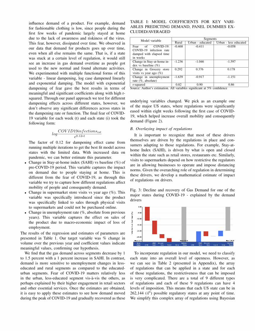
The results of the regression and estimates of parameters arepresented in Table 1. Our target variable was % change involume over the previous year and coefficient values indicatemeaningful values, confirming our hypothesis.
We find that the gas demand across segments decrease by 1to 1.5 percent with a 1 percent increase in SAHI. In contrast,demand is more sensitive to unemployment changes in less-educated and rural segments as compared to the educated-urban segments. Fear of COVID-19 matters relatively lessin the urban, less-educated segment vis-a-vis the others, asperhaps explained by their higher engagement in retail sectorsand other essential services. Once the estimates are obtained,it is easy to apply these estimates to see how demand movedduring the peak of COVID-19 and gradually recovered as these
TABLE I: MODEL COEFFICIENTS FOR KEY VARI-ABLES PREDICTING DEMAND, PANEL DUMMIES EX-CLUDED/AVERAGED
Model variable SegmentsRural Urban - educated Urban - less educated
Fear of COVID-19:COVID-19 infection ratedamped with elapsed timein weeks
-0.468 -0.411 -0.058
Change in Stay-at-home in-dex vs baseline (%)
-1.236 -1.046 -1.597
Change in Grocery storevisits vs year ago (%)
0.292 0.376 0.178
Change in unemploymentrate (%, absolute)
-1.639 -0.917 -1.151
r-squared 0.82 0.90 0.86Source: Author’s estimation. All variables significant at 5% confidence
underlying variables changed. We pick as an example oneof the major US states, where regulations were significantlyeased within eight weeks following the first case of COVID-19, which helped increase overall mobility and consequentlydemand (Figure 2).
B. Overlaying impact of regulations
It is important to recognize that most of these driversthemselves are driven by the regulations in place and con-sumers adapting to those regulations. For example, Stay-at-home Index (SAHI), is driven by what is open and closedwithin the state such as retail stores, restaurants etc. Similarly,visits to supermarkets depend on how restrictive the regulatorsare in allowing businesses to operate and impose distancingnorms. Given the overarching role of regulation in determiningthese drivers, we develop a mathematical estimate of impactof regulations on drivers.
Fig. 3: Decline and recovery of Gas Demand for one of themajor states during COVID-19 - explained by the demanddrivers
To incorporate regulation in our model, we need to classifyeach state into an overall level of openness. However, aswe can see in Table 2 (presented in Appendix), the arrayof regulations that can be applied in a state and for eachof those regulations, the restrictiveness that can be imposedis very complicated. There are a total of 9 different typesof regulations and each of these 9 regulations can have 4levels of imposition. This means that each US state can be in262,144 (49) possible regulatory states at any point of time.We simplify this complex array of regulations using Bayesian
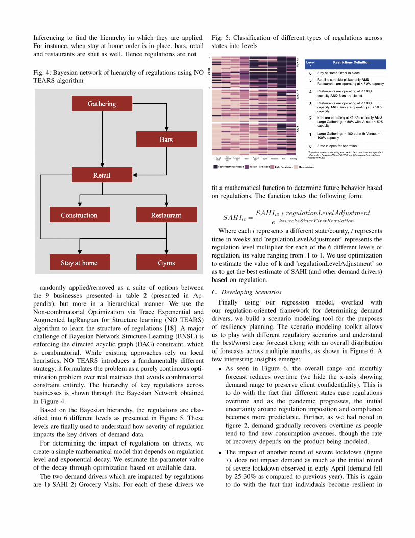
Inferencing to find the hierarchy in which they are applied.For instance, when stay at home order is in place, bars, retailand restaurants are shut as well. Hence regulations are not
Fig. 4: Bayesian network of hierarchy of regulations using NOTEARS algorithm
randomly applied/removed as a suite of options betweenthe 9 businesses presented in table 2 (presented in Ap-pendix), but more in a hierarchical manner. We use theNon-combinatorial Optimization via Trace Exponential andAugmented lagRangian for Structure learning (NO TEARS)algorithm to learn the structure of regulations [18]. A majorchallenge of Bayesian Network Structure Learning (BNSL) isenforcing the directed acyclic graph (DAG) constraint, whichis combinatorial. While existing approaches rely on localheuristics, NO TEARS introduces a fundamentally differentstrategy: it formulates the problem as a purely continuous opti-mization problem over real matrices that avoids combinatorialconstraint entirely. The hierarchy of key regulations acrossbusinesses is shown through the Bayesian Network obtainedin Figure 4.
Based on the Bayesian hierarchy, the regulations are clas-sified into 6 different levels as presented in Figure 5. Theselevels are finally used to understand how severity of regulationimpacts the key drivers of demand data.
For determining the impact of regulations on drivers, wecreate a simple mathematical model that depends on regulationlevel and exponential decay. We estimate the parameter valueof the decay through optimization based on available data.
The two demand drivers which are impacted by regulationsare 1) SAHI 2) Grocery Visits. For each of these drivers we
Fig. 5: Classification of different types of regulations acrossstates into levels
fit a mathematical function to determine future behavior basedon regulations. The function takes the following form:
SAHIit =SAHIi0 ∗ regulationLevelAdjustment
e−k∗weeksSinceFirstRegulation
Where each i represents a different state/county, t representstime in weeks and ’regulationLevelAdjustment’ represents theregulation level multiplier for each of the 6 different levels ofregulation, its value ranging from .1 to 1. We use optimizationto estimate the value of k and ’regulationLevelAdjustment’ soas to get the best estimate of SAHI (and other demand drivers)based on regulation.
C. Developing Scenarios
Finally using our regression model, overlaid withour regulation-oriented framework for determining demanddrivers, we build a scenario modeling tool for the purposesof resiliency planning. The scenario modeling toolkit allowsus to play with different regulatory scenarios and understandthe best/worst case forecast along with an overall distributionof forecasts across multiple months, as shown in Figure 6. Afew interesting insights emerge:
• As seen in Figure 6, the overall range and monthlyforecast reduces overtime (we hide the x-axis showingdemand range to preserve client confidentiality). This isto do with the fact that different states ease regulationsovertime and as the pandemic progresses, the initialuncertainty around regulation imposition and compliancebecomes more predictable. Further, as we had noted infigure 2, demand gradually recovers overtime as peopletend to find new consumption avenues, though the rateof recovery depends on the product being modeled.
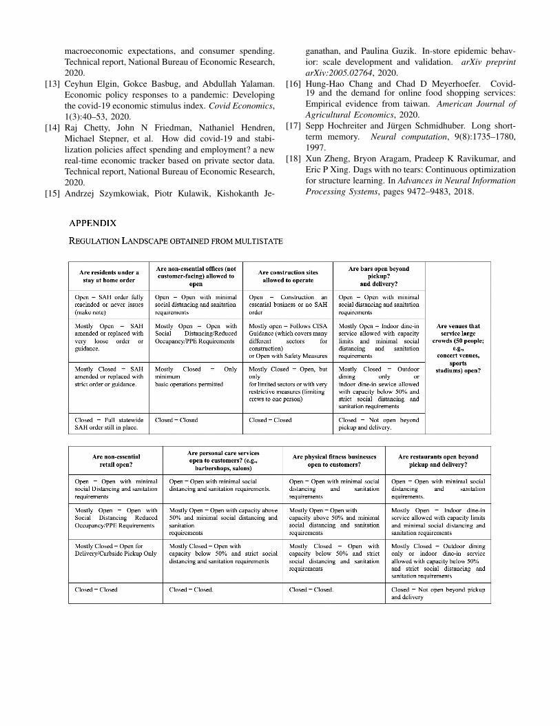
• The impact of another round of severe lockdown (figure7), does not impact demand as much as the initial roundof severe lockdown observed in early April (demand fellby 25-30% as compared to previous year). This is againto do with the fact that individuals become resilient in
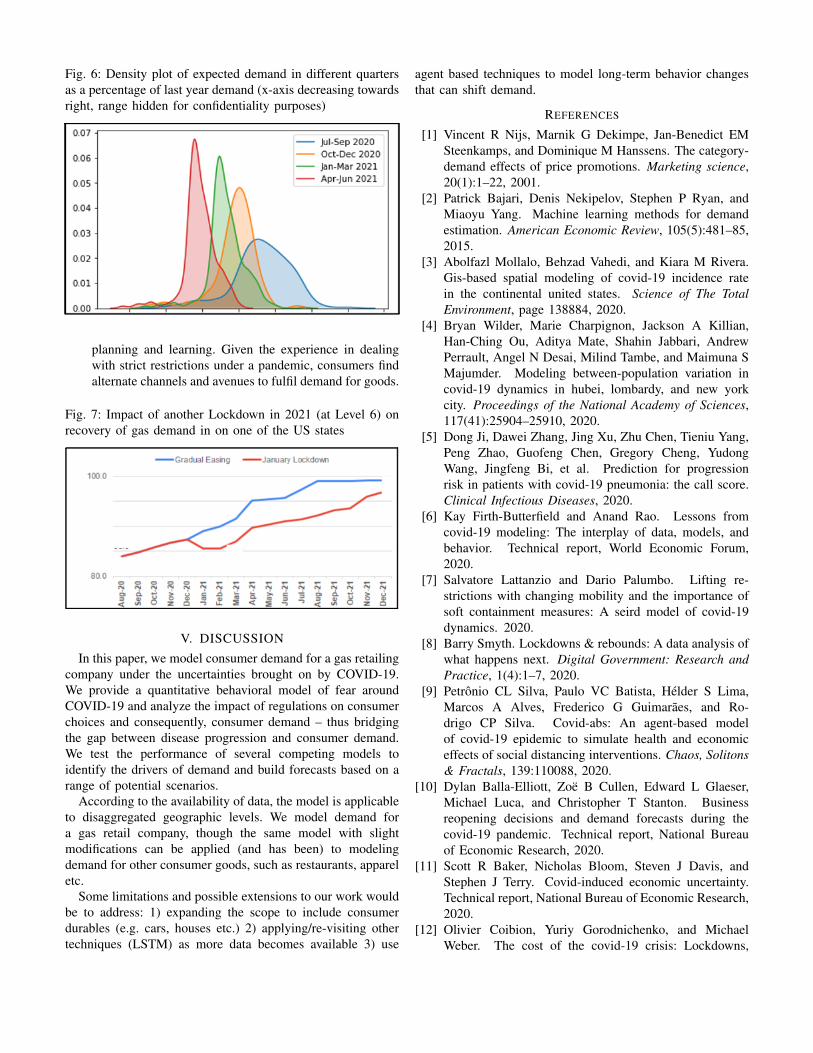
Fig. 6: Density plot of expected demand in different quartersas a percentage of last year demand (x-axis decreasing towardsright, range hidden for confidentiality purposes)
planning and learning. Given the experience in dealingwith strict restrictions under a pandemic, consumers findalternate channels and avenues to fulfil demand for goods.
Fig. 7: Impact of another Lockdown in 2021 (at Level 6) onrecovery of gas demand in on one of the US states
V. DISCUSSIONIn this paper, we model consumer demand for a gas retailing
company under the uncertainties brought on by COVID-19.We provide a quantitative behavioral model of fear aroundCOVID-19 and analyze the impact of regulations on consumerchoices and consequently, consumer demand – thus bridgingthe gap between disease progression and consumer demand.We test the performance of several competing models toidentify the drivers of demand and build forecasts based on arange of potential scenarios.
According to the availability of data, the model is applicableto disaggregated geographic levels. We model demand fora gas retail company, though the same model with slightmodifications can be applied (and has been) to modelingdemand for other consumer goods, such as restaurants, appareletc.
Some limitations and possible extensions to our work wouldbe to address: 1) expanding the scope to include consumerdurables (e.g. cars, houses etc.) 2) applying/re-visiting othertechniques (LSTM) as more data becomes available 3) use
agent based techniques to model long-term behavior changesthat can shift demand.
REFERENCES
[1] Vincent R Nijs, Marnik G Dekimpe, Jan-Benedict EMSteenkamps, and Dominique M Hanssens. The category-demand effects of price promotions. Marketing science,20(1):1–22, 2001.
[2] Patrick Bajari, Denis Nekipelov, Stephen P Ryan, andMiaoyu Yang. Machine learning methods for demandestimation. American Economic Review, 105(5):481–85,2015.
[3] Abolfazl Mollalo, Behzad Vahedi, and Kiara M Rivera.Gis-based spatial modeling of covid-19 incidence ratein the continental united states. Science of The TotalEnvironment, page 138884, 2020.
[4] Bryan Wilder, Marie Charpignon, Jackson A Killian,Han-Ching Ou, Aditya Mate, Shahin Jabbari, AndrewPerrault, Angel N Desai, Milind Tambe, and Maimuna SMajumder. Modeling between-population variation incovid-19 dynamics in hubei, lombardy, and new yorkcity. Proceedings of the National Academy of Sciences,117(41):25904–25910, 2020.
[5] Dong Ji, Dawei Zhang, Jing Xu, Zhu Chen, Tieniu Yang,Peng Zhao, Guofeng Chen, Gregory Cheng, YudongWang, Jingfeng Bi, et al. Prediction for progressionrisk in patients with covid-19 pneumonia: the call score.Clinical Infectious Diseases, 2020.
[6] Kay Firth-Butterfield and Anand Rao. Lessons fromcovid-19 modeling: The interplay of data, models, andbehavior. Technical report, World Economic Forum,2020.
[7] Salvatore Lattanzio and Dario Palumbo. Lifting re-strictions with changing mobility and the importance ofsoft containment measures: A seird model of covid-19dynamics. 2020.
[8] Barry Smyth. Lockdowns & rebounds: A data analysis ofwhat happens next. Digital Government: Research andPractice, 1(4):1–7, 2020.
[9] Petronio CL Silva, Paulo VC Batista, Helder S Lima,Marcos A Alves, Frederico G Guimaraes, and Ro-drigo CP Silva. Covid-abs: An agent-based modelof covid-19 epidemic to simulate health and economiceffects of social distancing interventions. Chaos, Solitons& Fractals, 139:110088, 2020.
[10] Dylan Balla-Elliott, Zoe B Cullen, Edward L Glaeser,Michael Luca, and Christopher T Stanton. Businessreopening decisions and demand forecasts during thecovid-19 pandemic. Technical report, National Bureauof Economic Research, 2020.
[11] Scott R Baker, Nicholas Bloom, Steven J Davis, andStephen J Terry. Covid-induced economic uncertainty.Technical report, National Bureau of Economic Research,2020.
[12] Olivier Coibion, Yuriy Gorodnichenko, and MichaelWeber. The cost of the covid-19 crisis: Lockdowns,
macroeconomic expectations, and consumer spending.Technical report, National Bureau of Economic Research,2020.
[13] Ceyhun Elgin, Gokce Basbug, and Abdullah Yalaman.Economic policy responses to a pandemic: Developingthe covid-19 economic stimulus index. Covid Economics,1(3):40–53, 2020.
[14] Raj Chetty, John N Friedman, Nathaniel Hendren,Michael Stepner, et al. How did covid-19 and stabi-lization policies affect spending and employment? a newreal-time economic tracker based on private sector data.Technical report, National Bureau of Economic Research,2020.
[15] Andrzej Szymkowiak, Piotr Kulawik, Kishokanth Je-
ganathan, and Paulina Guzik. In-store epidemic behav-ior: scale development and validation. arXiv preprintarXiv:2005.02764, 2020.
[16] Hung-Hao Chang and Chad D Meyerhoefer. Covid-19 and the demand for online food shopping services:Empirical evidence from taiwan. American Journal ofAgricultural Economics, 2020.
[17] Sepp Hochreiter and Jurgen Schmidhuber. Long short-term memory. Neural computation, 9(8):1735–1780,1997.
[18] Xun Zheng, Bryon Aragam, Pradeep K Ravikumar, andEric P Xing. Dags with no tears: Continuous optimizationfor structure learning. In Advances in Neural InformationProcessing Systems, pages 9472–9483, 2018.