Consumer Behaviour in Retail: Next Logical Purchase using Deep Neural Network

Ankur VermaSamya.ai

ankur.verma@samya.ai

AbstractPredicting future consumer behaviour is one of the most chal-lenging problems for large scale retail firms. Accurate predic-tion of consumer purchase pattern enables better inventoryplanning and efficient personalized marketing strategies. Op-timal inventory planning helps minimise instances of Out-of-stock/ Excess Inventory and, smart Personalized marketingstrategy ensures smooth and delightful shopping experience.Consumer purchase prediction problem has generally beenaddressed by ML researchers in conventional manners, eitherthrough recommender systems or traditional ML approaches.Such modelling approaches do not generalise well in predict-ing consumer purchase pattern. In this paper, we present ourstudy of consumer purchase behaviour, wherein, we estab-lish a data-driven framework to predict whether a consumeris going to purchase an item within a certain time frame usinge-commerce retail data. To model this relationship, we createa sequential time-series data for all relevant consumer-itemcombinations. We then build generalized non-linear modelsby generating features at the intersection of consumer, item,and time. We demonstrate robust performance by experiment-ing with different neural network architectures, ML models,and their combinations. We present the results of 60 mod-elling experiments with varying Hyperparameters along withStacked Generalization ensemble [25] and F1-Maximizationframework. We then present the benefits that neural networkarchitectures like Multi Layer Perceptron, Long Short TermMemory (LSTM), Temporal Convolutional Networks (TCN)[13] and TCN-LSTM [12] bring over ML models like Xg-boost [4] and RandomForest.

1 IntroductionConsumer behaviour insights have always been one of thekey business drivers for retail, given fast changing con-sumer needs. Existing trend, competitor pricing, item re-views, sales and marketing are some of the key factors driv-ing today’s consumer world in retail. While very little infor-mation is available on future variablities of the above factors,retailers do have large volumes of historical transactionaldata. Past study [5] has shown that retailers use conventionaltechniques with available data to model consumer purchase.While these help in estimating purchase pattern for loyalconsumers and high selling items with reasonable accuracy,they do not perform well for the long tail. Since multiple pa-rameters interact non-linearly to define consumer purchase

pattern, traditional models are not sufficient to achieve highaccuracy across thousands to millions of consumers.

Most retail/e-retail brands, plan their short term inven-tory (2-4 weeks ahead) based on consumer purchase pat-tern. Also, certain sales and marketing strategies like OfferPersonalization and personalized item recommendations aremade leveraging results of consumer purchase predictionsfor the near future. Given that every demand planner workson a narrow segment of item portfolio, there is a high vari-ability in choices that different planners recommend. Ad-ditionally, the demand planners might not get enough op-portunities to discuss their views and insights over theirrecommendations. Hence, subtle effects like cannibalization[21], and item-affinity remain unaccounted for. Such inef-ficiencies lead to a gap between consumer needs and itemavailability, resulting in the loss of business opportunities interms of consumer churn, and out-of-stock and excess in-ventory.

Our paper makes the following contributions -• We study and present the usefulness of applying various

deep learning architectures along with tree based machinelearning algorithms to predict the next logical item pur-chase at consumer level.

• We present the performance of individual models withvarying hyperparameter configurations.

• We implement stacked generalization framework [25] asan ensemble method where a new model learns to com-bine the predictions from multiple existing models.

• We design and implement F1-maximization algorithmwhich optimises for purchase probability cut-off at con-sumer level.

2 Related WorkIn the past few years, usefulness of various machine learn-ing methods for predicting consumer purchase pattern havebeen analyzed in the academia field and few of them are of-ten used by ML practitioners. In most cases many of thoseapproaches are based on extracting consumer’s latent char-acteristics from its past purchase behavior and applying sta-tistical and ML based formulations [6, 5]. Some previousstudies have analyzed the use of random forest and Xgboosttechniques to predict consumer retention, where past con-sumer behavior was used as potential explanatory variable

arX

iv:2

010.

0695

2v1

[cs

.LG

] 1

4 O

ct 2

020

for modelling such patterns. In one such study [15], the au-thors develop a model for predicting whether a consumerperforms a purchase in prescribed future time frame basedon historical purchase information such as the number oftransactions, time of the last transaction, and the relativechange in total spending of a consumer. They found gradientboosting to perform best over test data. We propose neuralnetwork architectures with entity embeddings [9] which out-perform the gradient boosting type of models like Xgboost[4].

From Neural Network architectures perspective, close toour work is Deep Neural Network Ensembles for Time Se-ries Classification [8]. In this paper, authors show how anensemble of multiple Convolutional Neural Networks canimprove upon the state-of-the-art performance of individ-ual neural networks. They use 6 deep learning classifiers in-cluding Multi Layer Perceptron, Fully Convolutional NeuralNetwork, Residual Network, Encoder [20], Multi-ChannelsDeep Convolutional Neural Networks [29] and Time Convo-lutional Neural Network [28]. The first three were originallyproposed in [24]. We propose the application of such archi-tectures in the consumer choice world and apply the conceptof entity embeddings [9] along with neural network architec-tures like Multi Layer Perceptron, Long Short Term Memory(LSTM), Temporal Convolutional Networks (TCN) [13] andTCN-LSTM [12].

3 MethodologyWe treat each relevant consumer-item as an individual objectand shape them into weekly time series data based on histor-ical transactions. In this setup, target value at each time step(week) takes a binary input, 1/0 (purchased/non purchased).Relevancy of the consumer-item is defined by items trans-acted by consumer during training time window. Positivesamples (purchased/1) are weeks where consumer did trans-act for an item, whereas Negative samples (non purchased/0)are the weeks where the consumer did not buy that item. Weapply sliding windows testing routine for generating out oftime results. The time series is split into 4 parts - train, vali-dation, test1, and test2 as shown in Table 1. All our modelsare built in a multi-object fashion, which allows the gradi-ent movement to happen across all consumer-item combina-tions split in batches. This enables cross-learning to happenacross consumers/items. We then perform Feature Engineer-ing over data splits to generate modelling features. Beloware some of the feature groups we perform our experimentswith:

• Datetime: We use transactional metrics at various tempo-ral cuts like week, month, etc. Datetime related featurescapturing seasonality and trend are also generated.

• Consumer-Item Profile: We use transactional metricsat different granularities like consumer, item, consumer-item, department and aisle. We also create features likeTime since first order, Time since last order, time gap be-tween orders, Reorder rates, Reorder frequency, Streak -user purchased the item in a row, Average position in thecart, Total number of orders.

Table 1: Modelling data splits

Data Split Specifications Consumer-Item combinations Max Time-Series lengthTrain Model training 50,872 46 weeks

Validation HyperParameter Optimization 50,888 2 weeksTest1 Stacked Generalization, F1-Maximization 50,899 2 weeksTest2 Reporting Accuracy Metrics 50,910 2 weeks

• Consumer-Item-Time Profile: We use transactionalmetrics at the intersection of consumer, item and time.We generate interactions capturing consumer behaviourtowards items at a given time.

• Lagged Offsets: We use statistical rolling operations likemean, median, quantiles, variance, kurtosis and skewnessover temporal regressors for different lag periods to gen-erate offsets.

The model we need to build, thus, should learn to identifysimilarly behaving time series across latent parameters, andtake into account consumer and item variations in comparingdifferent time series. A row in time series is represented by

ycit = f(it, ct, .., ct-n, ict, .., ict-n, dt, .., dt-n) (1)

where ycit is purchase prediction for consumer ’c’ for item’i’ at time ’t’. it denotes attributes of item ’i’ like category,department, brand, color, size, etc at time ’t’. ct denotes at-tributes of consumer ’c’ like age, sex and transactional at-tributes at time ’t’. ict denotes transactional attributes of con-sumer ’c’ towards item ’i’ at time ’t’. dt is derived from date-time to capture trend and seasonality at time ’t’. ’n’ is thenumber of time lags.

3.1 Loss FunctionSince we are solving Binary Classification problem, we be-lieve that Binary Cross-Entropy should be the most appro-priate loss function for training the models. We use the be-low formula to calculate Binary Cross-Entropy:

Hp = − 1N

∑Ni=1 y.log(p(y)) + (1− y).log(1− p(y))

(2)here Hp represents computed loss, y is the target value (la-bel), and p(y) is the predicted probability against the target.The BCELoss takes non-negative values. We can infer fromEquation 2 that Lower the BCELoss, better the Accuracy.

3.2 Model ArchitecturesAs mentioned earlier in this section, traditional machinelearning models are not really a suitable choice for mod-elling f (Equation 1) due to non-linear interaction betweenthe features. Hence, we work with tree based models likeRandomForest, Xgboost [4] to Deep learning models likeMulti Layer Perceptron (MLP), Long Short Term Memory(LSTM) and Temporal Convolutional Networks (TCN). Ar-chitectures of MLP, LSTM, TCN [13] and TCN-LSTM [12]models are shown in Figure 2, Figure 3, Figure 4 and Figure5 respectively. We briefly describe the architectures below.

• Entity Embeddings + Multi Layer Perceptron: MLP(Figure 2) is the simplest form of deep neural networksand was originally proposed in [24]. The architecture

contains three hidden layers fully connected to the out-put of its previous layer. The final layer is the sigmoidlayer which generates the probability. One disadvantageof MLP is that since the input time series is fully con-nected to the first hidden layer, the temporal informationin a time series is lost [7].

• Entity Embeddings + Long Short Term Memory:LSTM (Figure 3) is an architecture comprising of 2LSTM layers combined with entity embeddings. Thiscombination flows into 3 fully connected ReLU based lay-ers yielding to dense layer which has sigmoid activation.

• Entity Embeddings + Temporal Convolutional Net-work: TCN (Figure 4), originally proposed in [13] , isconsidered a competitive architecture yielding the best re-sults when evaluated over our experimental dataset. Thisnetwork comprises of 3 dilated Convolutional networkscombined with entity embeddings. Similar to LSTM, thisarchitecture, after convolving and concatenating flowsinto 3 fully connected ReLU based layers yielding todense layer which has sigmoid activation.

• Entity Embeddings + Long Short Term Memory-Temporal Convolutional Network: TCN-LSTM (Figure5) inherits the properties of LSTM and TCN in a fullyconnected network.

From data classification, Figure 1, we can see that data wassub-divided 4 groups:• Static Categorical: These are categorical features that do

not vary with time. This includes consumer attributes likesex, marital status and location along with different itemattributes like category, department and brand.

• Temporal Categorical: These are categorical featuresthat vary with time. It includes all the datetime relatedfeatures like week, month of year, etc.

• Static Continuous: These features are static but contin-uous. This includes certain consumer attributes like ageand weight, item attributes like size, and certain derivedfeatures like target encoded features.

• Temporal Continuous: These are time varying continu-ous features. All consumer and item related traditional at-tributes like number of orders, add to cart order, etc. fallsunder this bucket.

As mentioned earlier in this section, in all the above de-scribed neural network architectures, we learn the embed-dings [9] of the categorical features during training phase.We embed these attributes in order to compress their rep-resentations while preserving salient features, and capturemutual similarities and differences.

The consumer purchase pattern has huge variationin terms of time of purchase (weekday/weekends), ca-dence of purchase (days to months), purchased item types(dairy/meat/grocery/apparels/etc.) and brand loyalty (ten-dency to substitute items). Given such huge variations, it be-comes imperative to cross learn consumer behaviour fromsimilar consumer groups. To learn such relationships its im-portant to capture non-linear relationship between target andregressors at various levels. Tree based and Deep learning

Figure 1: Data classification for DNN Architectures

Figure 2: Multi Layer Perceptron (MLP)

models are chosen for their ability to model feature interac-tions (even if transient in time), and their ability to capturenon-linearity well.

Tree based models and MLP training uses lagged valuesof time varying regressors to capture temporal dependencies.LSTM, TCN and TCN-LSTM models are trained using en-tire life-cycle data of a time series (Consumer-Item) in se-quential manner. Details around dataset and features are ex-plained in section 4.

3.3 Hyperparameter TuningHyper-parameters of tree based models are optimized us-ing Bayesian Hyperparameter Optimization Technique, Hy-peropt [2]. For Deep learning, we use documented bestpractices along with our experimental results to choosemodel hyperparameters. Hyperparameter Optimization isperformed over validation dataset. We list some of the hy-perparameters along with the values we tune for Deep learn-ing models.

• Optimizer Parameters: RMSProp [1] and Adam areused as different trial configurations. The learning rate isexperimentally tuned to 1e-3. We also have weight decayof 1e-5 which helps a bit in model Regularization.

• Scheduler Parameters: CyclicLR [22] and ReduceL-ROnPlateau [27] Learning rates are used as different trialconfigurations. we use 1e-3 as max lr and 1e-6 as base lrfor cyclical learning rate along with the step size being thefunction of length of train loader. ReduceLROnPlateau istuned at 1e-6 as min lr.

• SWA: Stochastic Weight Averaging (SWA) [11] is usedto improve generalization across Deep Learning models.SWA performs an equal average of the weights traversedby SGD with a modified learning rate schedule. We use1e-3 as SWA learning rate.

Figure 3: Long Short Term Memory (LSTM)

Figure 4: Temporal Convolutional Network (TCN)

• Parameter Average: This is a method to average the neu-ral network parameters of n best model checkpoints posttraining, weighted by validation loss of respective check-points. The resulting model generalizes better than thosewith a single best checkpoint model for an unseen data.

Apart from the above parameters we also iterate to tune net-work parameters like number of epochs, batch size, numberof Fully Connected Layers, number of LSTM layers, con-vnet parameters (kernel size, dilations, padding) and embed-ding sizes for the categorical features. Binary Cross-Entropy2 is used as loss function for all the models. For sequencemodel [23], we also iterate with Dropout [10] and Batch-Norm [19] within networks. Hyperparameters used for Ma-chine learning models with Hyperopt [2] are :• Learning Rate: Range set to vary between 1e-2 to 5e-1.• Max Depth: Range set from 2 to 12 at step of 1.Apart from above hyperparameters, regularization parame-ters like Reg Lambda and Min Sample Leaf are also opti-mized using Hyperopt.

Deep learning models are built using deep learning frame-work PyTorch [16], and are trained on GCP instance con-

Figure 5: TCN-LSTM

taining 6 CPUs and a single GPU. Scikit-learn [17] is usedfor Tree based models like RandomForest and Xgboost [4].For Neural Network Architectures, we save model weightsof the best checkpoint, so that we may access the learnedentity embeddings and other model weights if required. Asdescribed in Table 2, we build a total of 60 models, 12 dif-ferent configurations for each of 4 Deep Learning modelsand 6 best trials from Hyperopt [2] for each of 2 MachineLearning models.

3.4 Stacked Generalization EnsembleStacked generalization or Stacking [25] is an ensemblemethod where a new model learns how to best combine thepredictions from multiple existing models. This is achievedby training an entirely new model using contributions fromeach submodel. We use weighted K-best model as Stackerfor combining k submodels (candidates) out of total 60trained models. We iterate with different values of k rang-ing from 3 to 25 as presented in Table 6 . test1 BCELossof submodels is used for weight initialization for the stackermodels. For learning optimal weights of submodels, we min-imise test1 BCELoss of the stacker model using gradient de-scent [18], stacking function can be described as:

ycit =∑k

j=1 wj × pcitj (3)

where ycit is the stacked probability for consumer ’c’ foritem ’i’ at time ’t’. k represents the number of candidatesshortlisted for stacking, pcitj represents the prediction proba-bility for consumer ’c’ for item ’i’ at time ’t’ by jth submodel.wj is the weight for jth submodel.

3.5 F1-MaximizationPost stacking, we optimize for purchase probability thresh-old based on probability distribution at a consumer level us-ing F1-Maximization. This enables optimal thresholding ofconsumer level probabilities to maximize F1 measure [14].To illustrate the above, let us say we generated purchaseprobabilities for ’n’ items out of ’b’ actually purchased itemsby consumer ’c’. Now, let us visualize the actuals (4) and

predictions (5) of ’n’ predicted items for consumer ’c’.

Ac = [a1, a2, .., an] ∀ aj ∈ {0,1} (4)

P c = [p1, p2, .., pn] ∀ pj ∈ [0, 1] (5)Ac represents the actuals for consumer ’c’, with aj being 1/0(purchased/non purchased). Pc represents the predictions forconsumer ’c’ for the respective item, with pj being proba-bility value. ’n’ represents total items for which the modelgenerated purchase probabilities for consumer ’c’. Now weapply Decision rule D() which converts probabilities to bi-nary predictions, as described below in Equation 6.

D(Prc) : P c1 x n → P ’

c1 x n : p’

j =

{1 pj ≥ Prc

0 Otherwise(6)

P ’c = [p’

1, p’2, .., p

’n] ∀ p’

j ∈ {0,1} (7)

k =∑n

i=1 p’i (8)

Prc is the probability cut-off to be optimized for maximizingF1 measure [14] for consumer ’c’. Decision rule D() convertsprobabilities Pc to binary predictions P’

c such that if pj isless than Prc then p’

j equals 0, otherwise 1. ’k’ is the sum ofpredictions generated post applying Decision rule D(). Nowwe solve for F1 measure using equations and formulae de-scribed below.

V Prc = P ’c × Ac

T ⇒(p’

1 .. p’n)×

(a1..an

)(9)

Precisionc =V Prck and Recallc =

V Prcb

(10)

F 1c =2×Precisionc×RecallcPrecisionc+Recallc

⇒ 2 ∗ V Prck+b

(11)

VPrc represents the number of items with purchase probabil-ities greater than Prc which were actually purchased (TruePositives). As can be seen, Formulae 10 and 11 are used tocalculate Precision, Recall and F1-score for consumer ’c’.

maxV Prc

2 ∗ V Prc

k + b, subject to: Prc ∈ [0, 1] (12)

Equation 12 represents the optimization function we solveto generate purchase predictions (1/0) for each consumer.

4 Experiments and ResultsWe use transactional data from instacart kaggle challengeto train all our models (sample data 6). From sample datawe can see that data contains transactional details includingorder id, add to cart order, date of transaction, aisle id anddepartment id for each consumer-item transaction. As de-scribed in Table 1, we utilize 1 year data for each consumer-item combination, which then gets split into train, validation,test1 and test2 as per our validation strategy. We generateconsumer-item-week level data with purchase/ non purchasebeing the target, and use this data to train all our models.

4.1 Experiment SetupsWe start with exploratary data analysis, looking at the datafrom various cuts. We study the variations of different fea-tures with our target (purchase/ non purchase). Some of ourstudies are density of consumers versus basket size (Fig-ure 8), reorder visualization of items across departments(Figure 7), variation of reorder probability with add to cartorder (Figure 9), order probability variations at differenttemporal cuts like week, month and quarter, transactionalmetrics like total orders, total reorders, recency, gap be-tween orders, at both consumer and item levels. We thenperform multiple experiments with the above mentioned fea-tures and different hyperparameter configurations to landat reasonable hyperparameters to perform final experimentsand present our results.

4.2 Results and ObservationsTables 3 and 4 show the experimental results obtained acrossmodels with different hyperparameter configurations. Ta-ble 3 contains the Deep Learning Experiment setup resultsand Table 4 has Machine Learning model results. Frommodel performance perspective, it is observed that Tempo-ral Convolution Network (TCN) has least average BCELossof 0.0251, approximately 2% better than the second bestmodel which is Multi Layer Perceptron (MLP) having av-erage BCELoss of 0.0256. Table 5 presents the compar-ative analysis of average scores across all models. Also,we observe in Table 5 that Deep Learning models out per-form Machine Learning models including Xgboost and Ran-domForest in terms of accuracy. Average BCELoss of DeepLearning model is approximately about 0.0266 , whereas forMachine Learning models its approximately about 0.0388.From hyperparameter configuration perspective, we observethat RMSprop and CyclicLR emerged as the winners as Op-timizer and Scheduler respectively (from Table 3). 7 out of12 times, the combination of RMSprop and CyclicLR (outof 3 possible combinations) generate the best result.

We also present the effectiveness of combining submodelpredictions and F1-Maximization. Table 6 outlines the re-sults of stacking at different values of K for Weighted K-Best stacker model. We realise the best accuracy or leastBCELoss of 0.0242 at K = 3. To analyse our probability val-ues post stacking, we plot the probability distributions forboth labels of the target, as can be seen in Figure 10. Finallywe apply F1-Maximization over stacked probability valuesso as to generate purchase predictions. F1-Score Optimizerhelps strike balance between Precision and Recall [3]. PostF1-Maximization we observe that Precision, Recall and F1-Score are close enough for all data splits, as can be seen inTable 7. F1-Score of our model over unseen data (test2) is0.4109 (Table 7).

4.3 Industrial ApplicationsThe Next Logical Purchase framework has multiple applica-tions in retail/e-retail industry. Some of them include:

• Personalized Marketing: With prior knowledge of nextlogical purchase, accurate item recommendations and op-timal offer rollouts can be made at consumer level. This

Table 2: Model Specifications

Model Type Trials Model HyperParameters Loss FunctionsMLP 12 Optimizer, Scheduler, SWA, Parameter Averaging, Feature Groups, FC Layers BCELoss

LSTM 12 Optimizer, Scheduler, SWA, Parameter Averaging, Feature Groups, FC Layers, LSTM Layers BCELossTCN 12 Optimizer, Scheduler, SWA, Parameter Averaging, Feature Groups, FC Layers, Convolution Parameters BCELoss

TCN-LSTM 12 Optimizer, Scheduler, SWA, Parameter Averaging, Feature Groups, FC Layers, LSTM, Convolution Parameters BCELossXgboost 6 Learning rate, Tree Depth, Regularization parameters BCELoss

RandomForest 6 Tree Depth, Evaluation Metrics, Regularization parameters BCELoss

Figure 6: Sample Dataset

Table 3: BCELoss of Test2 for 12 Trials of Deep Learning Models

Trial Optimizer Scheduler SWA Parameter Avg MLP LSTM TCN TCN-LSTM1 RMSprop ReduceLROnPlateau True False 0.0276 0.0306 0.0249 0.03072 RMSprop CyclicLR True False 0.0708 0.0269 0.0269 0.03483 Adam ReduceLROnPlateau True False 0.0295 0.0303 0.0667 0.03374 RMSprop ReduceLROnPlateau False False 0.0297 0.0275 0.0364 0.07595 RMSprop CyclicLR False False 0.0250 0.0306 0.0600 0.02866 Adam ReduceLROnPlateau False False 0.0360 0.0302 0.0590 0.03097 RMSprop ReduceLROnPlateau False True 0.0293 0.0432 0.0453 0.03818 RMSprop CyclicLR False True 0.0245 0.0378 0.0569 0.02629 Adam ReduceLROnPlateau False True 0.0700 0.0491 0.0610 0.0382

10 RMSprop ReduceLROnPlateau True True 0.0356 0.0364 0.0238 0.030911 RMSprop CyclicLR True True 0.0420 0.0377 0.0284 0.026912 Adam ReduceLROnPlateau True True 0.0321 0.0306 0.0547 0.0305

Table 4: BCELoss of Test2 for 6 best Trials of ML Models

Trial HyperParameter Xgboost RandomForest1 HyperOpt 0.0332 0.05262 HyperOpt 0.0364 0.04793 HyperOpt 0.0347 0.04164 HyperOpt 0.0364 0.04495 HyperOpt 0.0335 0.04596 HyperOpt 0.0339 0.0578

will enable a seamless and delightful consumer shoppingexperience.

• Inventory Planning: Consumer preference model canalso be used in better short term inventory planning (2-4 weeks), which is largely dependant over what consumeris going to purchase in the near future.

Table 5: BCELoss mean of top 3 trials across data splits

Model Type Val BCELoss Test1 BCELoss Test2 BCELossMLP 0.0405 0.0289 0.0256

LSTM 0.0373 0.0293 0.0282TCN 0.0368 0.0292 0.0251

TCNLSTM 0.0368 0.0304 0.0273Xgboost 0.0352 0.0318 0.0335

RandomForest 0.0437 0.0389 0.0441

• Assortment Planning: In retail stores, consumer choicestudy can be used to optimize the store layout with rightproduct placement over right shelf.

5 ConclusionWe have presented our study of the consumer purchase be-haviour in the context of large scale e-retail. We have shownthat careful feature engineering when used in conjunction

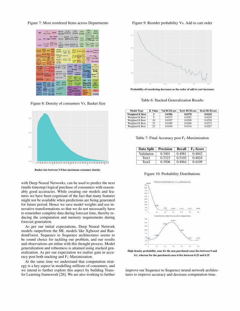
Figure 7: Most reordered Items across Departments

Figure 8: Density of consumers Vs. Basket Size

Basket size between 5-8 has maximum consumer density

with Deep Neural Networks, can be used to predict the next(multi-timestep) logical purchase of consumers with reason-ably good accuracies. While creating our models and fea-tures we have been cognizant of the fact that many featuresmight not be available when predictions are being generatedfor future period. Hence we save model weights and use in-novative transformations so that we do not necessarily haveto remember complete data during forecast time, thereby re-ducing the computation and memory requirements duringforecast generation.

As per our initial expectations, Deep Neural Networkmodels outperform the ML models like Xgboost and Ran-domForest. Sequence to Sequence architectures seems tobe sound choice for tackling our problem, and our resultsand observations are inline with this thought process. Modelgeneralization and robustness is attained using stacked gen-eralization. As per our expectation we realize gain in accu-racy post both stacking and F1-Maximization.

At the same time we understand that computation strat-egy is a key aspect in modelling millions of consumers, andwe intend to further explore this aspect by building Trans-fer Learning framework [26]. We are also working to further

Figure 9: Reorder probability Vs. Add to cart order

Probability of reordering decreases as the order of add to cart increases

Table 6: Stacked Generalization Results

Model Type K Value Val BCELoss Test1 BCELoss Test2 BCELossWeighted K Best 3 0.0386 0.0278 0.0242Weighted K Best 5 0.0373 0.0282 0.0245Weighted K Best 10 0.0397 0.0290 0.0258Weighted K Best 15 0.0389 0.0296 0.0272Weighted K Best 25 0.0394 0.0316 0.0287

Table 7: Final Accuracy post F1-Maximization

Data Split Precision Recall F1-ScoreValidation 0.3401 0.4981 0.4042

Test1 0.3323 0.5103 0.4024Test2 0.3506 0.4964 0.4109

Figure 10: Probability Distributions

High density probability zone for the non purchased cases lies between 0 and0.1, whereas for the purchased cases it lies between 0.25 and 0.35

improve our Sequence to Sequence neural network architec-tures to improve accuracy and decrease computation time.

6 AcknowledgementsThe authors would like to thank Yadunath Gupta for hiscontributions towards Neural network architecture improve-ments. Siddharth Shahi, Deepinder Singh Dhingra and AnkitJain for helpful discussions and insights over the methodol-ogy and implementation.

References[1] Bengio, Y.; and CA, M. 2015. Rmsprop and equili-

brated adaptive learning rates for nonconvex optimiza-tion. corr abs/1502.04390 .

[2] Bergstra, J.; Yamins, D.; and Cox, D. D. 2013. Hyper-opt: A python library for optimizing the hyperparame-ters of machine learning algorithms. In Proceedings ofthe 12th Python in science conference, volume 13, 20.Citeseer.

[3] Buckland, M.; and Gey, F. 1994. The relationship be-tween recall and precision. Journal of the Americansociety for information science 45(1): 12–19.

[4] Chen, T.; and Guestrin, C. 2016. Xgboost: A scalabletree boosting system. In Proceedings of the 22nd acmsigkdd international conference on knowledge discov-ery and data mining, 785–794.

[5] Choudhury, A. M.; and Nur, K. 2019. A MachineLearning Approach to Identify Potential CustomerBased on Purchase Behavior. In 2019 InternationalConference on Robotics, Electrical and Signal Pro-cessing Techniques (ICREST), 242–247. IEEE.

[6] Fader, P. S.; and Hardie, B. G. 2009. Probability mod-els for customer-base analysis. Journal of interactivemarketing 23(1): 61–69.

[7] Fawaz, H. I.; Forestier, G.; Weber, J.; Idoumghar, L.;and Muller, P.-A. 2019. Deep learning for time seriesclassification: a review. Data Mining and KnowledgeDiscovery 33(4): 917–963.

[8] Fawaz, H. I.; Forestier, G.; Weber, J.; Idoumghar, L.;and Muller, P.-A. 2019. Deep neural network ensem-bles for time series classification. In 2019 Interna-tional Joint Conference on Neural Networks (IJCNN),1–6. IEEE.

[9] Guo, C.; and Berkhahn, F. 2016. Entity em-beddings of categorical variables. arXiv preprintarXiv:1604.06737 .

[10] Hinton, G. E.; Srivastava, N.; Krizhevsky, A.;Sutskever, I.; and Salakhutdinov, R. R. 2012. Im-proving neural networks by preventing co-adaptationof feature detectors. arXiv preprint arXiv:1207.0580 .

[11] Izmailov, P.; Podoprikhin, D.; Garipov, T.; Vetrov, D.;and Wilson, A. G. 2018. Averaging weights leads towider optima and better generalization. arXiv preprintarXiv:1803.05407 .

[12] Karim, F.; Majumdar, S.; Darabi, H.; and Chen, S.2017. LSTM fully convolutional networks for time se-ries classification. IEEE access 6: 1662–1669.

[13] Lea, C.; Vidal, R.; Reiter, A.; and Hager, G. D. 2016.Temporal convolutional networks: A unified approachto action segmentation. In European Conference onComputer Vision, 47–54. Springer.

[14] Lipton, Z. C.; Elkan, C.; and Naryanaswamy, B. 2014.Optimal thresholding of classifiers to maximize F1measure. In Joint European Conference on MachineLearning and Knowledge Discovery in Databases,225–239. Springer.

[15] Martınez, A.; Schmuck, C.; Pereverzyev Jr, S.; Pirker,C.; and Haltmeier, M. 2020. A machine learningframework for customer purchase prediction in thenon-contractual setting. European Journal of Opera-tional Research 281(3): 588–596.

[16] Paszke, A.; Gross, S.; Chintala, S.; Chanan, G.; Yang,E.; DeVito, Z.; Lin, Z.; Desmaison, A.; Antiga, L.; andLerer, A. 2017. Automatic differentiation in pytorch .

[17] Pedregosa, F.; Varoquaux, G.; Gramfort, A.; Michel,V.; Thirion, B.; Grisel, O.; Blondel, M.; Prettenhofer,P.; Weiss, R.; Dubourg, V.; et al. 2011. Scikit-learn:Machine learning in Python. the Journal of machineLearning research 12: 2825–2830.

[18] Ruder, S. 2016. An overview of gradient descent opti-mization algorithms. arXiv preprint arXiv:1609.04747.

[19] Santurkar, S.; Tsipras, D.; Ilyas, A.; and Madry, A.2018. How does batch normalization help optimiza-tion? In Advances in Neural Information ProcessingSystems, 2483–2493.

[20] Serra, J.; Pascual, S.; and Karatzoglou, A. 2018. To-wards a Universal Neural Network Encoder for TimeSeries. In CCIA, 120–129.

[21] Shah, J.; and Avittathur, B. 2007. The retailer multi-item inventory problem with demand cannibalizationand substitution. International journal of productioneconomics 106(1): 104–114.

[22] Smith, L. N. 2017. Cyclical learning rates for train-ing neural networks. In 2017 IEEE Winter Conferenceon Applications of Computer Vision (WACV), 464–472.IEEE.

[23] Sutskever, I.; Vinyals, O.; and Le, Q. V. 2014. Se-quence to sequence learning with neural networks. InAdvances in neural information processing systems,3104–3112.

[24] Wang, Z.; Yan, W.; and Oates, T. 2017. Time seriesclassification from scratch with deep neural networks:A strong baseline. In 2017 International joint confer-ence on neural networks (IJCNN), 1578–1585. IEEE.

[25] Wolpert, D. H. 1992. Stacked generalization. Neuralnetworks 5(2): 241–259.

[26] Yosinski, J.; Clune, J.; Bengio, Y.; and Lipson, H.2014. How transferable are features in deep neural net-works? In Advances in neural information processingsystems, 3320–3328.

[27] Zaheer, M.; Reddi, S.; Sachan, D.; Kale, S.; and Ku-mar, S. 2018. Adaptive methods for nonconvex opti-mization. In Advances in neural information process-ing systems, 9793–9803.

[28] Zhao, B.; Lu, H.; Chen, S.; Liu, J.; and Wu, D. 2017.Convolutional neural networks for time series classifi-cation. Journal of Systems Engineering and Electron-ics 28(1): 162–169.

[29] Zheng, Y.; Liu, Q.; Chen, E.; Ge, Y.; and Zhao,J. L. 2014. Time series classification using multi-channels deep convolutional neural networks. In In-ternational Conference on Web-Age Information Man-agement, 298–310. Springer.