CONSUMER BEHAVIOR AND

TRAVEL MODE CHOICES

DRAFT Final Report

Please do not distribute or quote without permission

CONSUMER BEHAVIOR AND TRAVEL MODE

CHOICES

by

Professor Kelly J. Clifton

Christopher Muhs

Sara Morrissey

Tomás Morrissey

Kristina Currans

Chloe Ritter

for

Oregon Transportation Research

and Education Consortium (OTREC)

P.O. Box 751

Portland, OR 97207

November 2012

SI* (MODERN METRIC) CONVERSION FACTORS

APPROXIMATE CONVERSIONS TO SI UNITS APPROXIMATE CONVERSIONS FROM SI UNITS

Symbol When You Know Multiply By To Find Symbol Symbol When You Know Multiply By To Find Symbol

LENGTH LENGTH

in inches 25.4 millimeters mm mm millimeters 0.039 inches in

ft feet 0.305 meters m m meters 3.28 feet ft

yd yards 0.914 meters m m meters 1.09 yards yd

mi miles 1.61 kilometers km km kilometers 0.621 miles mi

AREA AREA

in2 square inches 645.2 millimeters squared mm2 mm2 millimeters squared 0.0016 square inches in2

ft2 square feet 0.093 meters squared m2 m2 meters squared 10.764 square feet ft2

yd2 square yards 0.836 meters squared m2 ha hectares 2.47 acres ac

ac acres 0.405 hectares ha km2 kilometers squared 0.386 square miles mi2

mi2 square miles 2.59 kilometers squared km2 VOLUME

VOLUME mL milliliters 0.034 fluid ounces fl oz

fl oz fluid ounces 29.57 milliliters mL L liters 0.264 gallons gal

gal gallons 3.785 liters L m3 meters cubed 35.315 cubic feet ft3

ft3 cubic feet 0.028 meters cubed m3 m3 meters cubed 1.308 cubic yards yd3

yd3 cubic yards 0.765 meters cubed m3 MASS

NOTE: Volumes greater than 1000 L shall be shown in m3. g grams 0.035 ounces oz

MASS kg kilograms 2.205 pounds lb

oz ounces 28.35 grams g Mg megagrams 1.102 short tons (2000 lb) T

lb pounds 0.454 kilograms kg TEMPERATURE (exact)

T short tons (2000 lb) 0.907 megagrams Mg C Celsius temperature 1.8 + 32 Fahrenheit F

TEMPERATURE (exact)

jan F Fahrenheit

temperature

5(F-32)/9 Celsius temperature C

* SI is the symbol for the International System of Measurement (4-7-94 jbp)

iii

ACKNOWLEDGEMENTS

The authors would like to thank the businesses that participated in this study. This project was

funded by Oregon Transportation Research and Education Consortium (OTREC), the Portland

Development Commission (PDC), Travel Oregon, and Bikes Belong. Additional advice and

assistance was received from the Portland Bureau of Transportation (PBOT). We would also like

to thank the various business establishments that allowed us to survey their patrons.

DISCLAIMER

The contents of this report reflect the views of the authors, who are solely responsible for the

facts and the accuracy of the material and information presented herein. This document is

disseminated under the sponsorship of the U.S. Department of Transportation University

Transportation Centers Program and Portland State University in the interest of information

exchange. The U.S. Government and Portland State University assume no liability for the

contents or use thereof. The contents do not necessarily reflect the official views of the U.S.

Government or Portland State University. This report does not constitute a standard,

specification, or regulation.

iv

TABLE OF CONTENTS

EXECUTIVE SUMMARY ...................................................................................................... VI

INTRODUCTION ................................................................................................. 1 CHAPTER 1

LITERATURE REVIEW ..................................................................................... 3 CHAPTER 2

DATA COLLECTION METHODOLOGY ....................................................... 7 CHAPTER 3

ESTABLISHMENT TYPES & SITE SELECTION .................................................................. 7 CUSTOMER SURVEYS ......................................................................................................... 10 BUILT ENVIRONMENT DATA ............................................................................................ 13

SUMMARY .............................................................................................................................. 17

ANALYSIS AND RESULTS .............................................................................. 18 CHAPTER 4

SUMMARY STATISTICS ....................................................................................................... 18 MODELS OF MODE SHARES AT THE ESTABLISHMENT LEVEL ................................ 27

MODELS OF SPENDING AT THE INDIVIDUAL LEVEL .................................................. 30 SUMMARY .............................................................................................................................. 38

CONCLUSIONS .................................................................................................. 39 CHAPTER 5

DISCUSSION ........................................................................................................................... 39 FUTURE CONSIDERATIONS ............................................................................................... 42

REFERENCES .................................................................................................... 44 CHAPTER 6

APPENDICES ............................................................................................................................. 47 APPENDIX A: LONG SURVEY ............................................................................................. 48

APPENDIX B: SHORT SURVEY ........................................................................................... 51

APPENDIX C: GROCERY STORE SURVEY ....................................................................... 52 APPENDIX D: SITE DATA COLLECTION TABLE ............................................................ 53

v

LIST OF TABLES

Table 3-1. Establishments Surveyed by Area and Land Use Type................................................. 7 Table 3-2. Survey Sample Size ..................................................................................................... 11 Table 3-3. Demographic Characteristics and Transportation Mode of Long Survey Sample ...... 11 Table 3-4. Demographic Characteristics of Supermarket Sample ................................................ 13

Table 3-5. Built Environment Measures and Sources .................................................................. 15 Table 3-6. Average Site Characteristics of Establishments .......................................................... 16 Table 3-7. Correlations between Built Environment Measures .................................................... 17 Table 4-1. Percentage of Trips Shorter than 3 miles .................................................................... 22 Table 4-2 Consumer Expenditures and Frequency of Trips ......................................................... 26

Table 4-3. Model results: bicycling mode share at establishment level ....................................... 28

Table 4-4. Model results: non-automobile mode share at establishment level ............................. 30 Table 4-5. Spending per Trip Model Results ................................................................................ 34

LIST OF FIGURES

Figure 3-1. Locations of Survey Establishments ............................................................................ 9 Figure 4-1. Observed Mode Share ................................................................................................ 19 Figure 4-2. Mode shares of Survey Establishments...................................................................... 21

Figure 4-3. Trip Lengths, Origin to Establishment ....................................................................... 22 Figure 4-4. Average trip distance from origin to establishment ................................................... 23

Figure 4-5 Average Consumer Expenditures per Trip .................................................................. 24 Figure 4-6 Average Consumer Trips per Month........................................................................... 25 Figure 4-7 Estimated Average Spending per Month .................................................................... 25 Figure 4-8. Bicycle mode share model results .............................................................................. 28 Figure 4-9. Non-automobile Mode Share Model Results ............................................................. 30

Figure 4-10. Significant Factors of Spending per Trip at Restaurants and Drinking

Establishments ...................................................................................................................... 36 Figure 4-11. Significant Factors of Spending per Trip at Convenience Stores ............................ 36

Figure 4-12 Significant Factors of Spending per Trip at Supermarkets ....................................... 37 Figure 5-1. Time-of-day Distribution of Travel Modes................................................................ 42

vi

EXECUTIVE SUMMARY

This study represents a first attempt to answer a few of the questions that have arisen concerning

multimodal transportation investments and the impacts of mode shifts on the business

community. This research aims to merge the long history of scholarly work that examines the

impacts of the built environment on non-work travel with the relatively new interest in consumer

spending by mode of travel. This empirical study of travel choices and consumer spending across

89 businesses in the Portland metropolitan area shows there are important differences between

the amounts customers spend on average at various businesses by their mode of travel. However,

these differences become less pronounced when we control for demographics of the customer

and other attributes of the trip. This study of consumer spending and travel choices has some

compelling findings that suggest some key spending and frequency differences by mode of travel

that will likely invigorate the discussion of the economic impacts of these modes.

Key findings are the following:

Bicyclists, pedestrians, and transit riders are competitive consumers: when demographics

and socioeconomics are controlled for, mode choice does not have a statistically

significant impact on consumer spending at convenience stores, drinking establishments,

and restaurants. When trip frequency is accounted for, the average monthly expenditures

by customer modes of travel reveal that bicyclists, transit users, and pedestrians are

competitive consumers and for all businesses except supermarkets, spend more, on

average than those who drive.

The built environment matters: we support previous literature and find that residential

and employment density, the proximity to rail transit, the presence of bike infrastructure,

and the amount of automobile and bicycle parking are all important in explaining the use

of non-automobile modes. In particular, provision of bike parking and bike corrals are

significant predictors of bike mode share at the establishment level.

Other findings lend more insight into the relationship between consumer behavior and travel

choices. For the non-work destinations studied, the automobile remains the dominant mode of

travel. Patrons are largely arriving by private vehicle to most of the destinations in this study,

particularly to grocery stores where larger quantities of goods tend to be purchased. But, high

non-automobile mode shares and short travel distances exist in areas of concentrated urban

activity.

In sum, this study provides some empirical evidence to answer the questions of business owners

about how mode shifts might impact their market shares and revenues. More work is needed to

better understand the implications of future changes and to provide a robust assessment of the

returns on these investments and their economic impacts.

1

Introduction Chapter 1

American retailing and service sectors have been accommodating the automobile since its

widespread adoption after World War II. The built environment in many communities was

modified to support the automobile, often to the exclusion of other modes of travel. As a result,

business owners often anticipate that patrons will travel by private vehicle and sometimes

express concerns about policies to reduce automobile travel or that promote changes to the built

environment that favor the use of non-automobile modes. Merchants may be concerned that

mode shifts away from travel by private vehicle will lead to decreased sales revenue. Currently,

there is little research evidence to prove that these fears are unfounded.

For the last thirty years, the policy question that has dominated much of travel behavior research

is the anticipated demand associated with levels of infrastructure investment and built

environment characteristics. Great progress has been made in this area and while many questions

still remain, there is a rich and long literature to help inform policy and plans. Cities across the

US are making new or expanded investments in bicycling, transit, and walking infrastructure,

motivated by the anticipated benefits associated with decreases in automobile use and associated

fuel and emissions reductions, improvements to societal health, increased transportation choices

and greater equity for all system users.

Amid the ongoing discussion regarding the evidence supporting these benefits, new concerns

have arisen about the economic impacts of these investments. The debates around increases in

non-automobile transportation options have expanded to question how these investments impact

businesses. While there is a wealth of information that examines the connections between the

built environment and mode choices, information that contributes to a discussion about returns

on investments in non-automobile infrastructure is lacking. This study seeks to fill that gap by

examining the links between transportation choices and consumer spending and patronage.

Here we are guided by the following objectives:

1. Quantify the transportation mode shares of customers for a variety of business types,

locations and transportation contexts

2. Test the associations of these establishment-level mode shares and attributes of the built

environment

3. Examine the links between consumer spending and frequency of visits at these businesses

and mode of travel while controlling for other factors

To achieve these objectives, this study makes use of intercept surveys of local business patrons

and built environment data to inform its analysis. The locations included in this study were

chosen based upon the characteristics of the individual business, area demographics, land

use/built environment context, and the transportation environment. Analysis of these data at both

the establishment and individual patron level will provide important evidence about important

2

differences in customer transportation, spending and patronage to help address these emerging

questions about economic impacts.

This report is organized as follows. A literature review summarizes the current state of the

knowledge about the economic impacts of various modes, with an emphasis on consumer

behavior. Then, the data used in this study and the methods used to collect them are described.

Next, we present the results of our data analysis and key study findings. The report concludes

with a discussion of the implications of our findings for planning and policy, study limitations,

and suggestions for future work. Supporting documentation is provided in the Appendices.

3

Literature Review Chapter 2

The following review begins by briefly summarizing the academic and professional studies

examining travel behavior and the built environment, specifically focusing on non-work travel.

Then, we present the few available studies that discuss consumer spending related to travel mode

choice, with a section devoted to travel to supermarket. Finally, we discuss concerns and

perceptions of business owners about how their patrons access their store.

THE CURRENT BUILT ENVIRONMENT

As automobile use increased after WWII, retailers expanded their conception of market area

based on the speed and range of automobiles and delivery trucks, resulting in fewer but larger

establishments located along major thoroughfares with an ample supply of off-street automobile

parking (Handy, 1993). At the same time, conventional land use policy and development

practices throughout the 20th century encouraged low-density, suburban housing developments.

This resulted in increased separation of residential areas and shopping districts, making

accessing retail locations by non-automobile mode inconvenient and sometimes unsafe. The

result is a retail built environment that tends to favor car accessibility over other modes of

transportation (Grant & Perrot, 2011).

Although the current US built environment caters to automobile use in most communities, it can

be restructured to promote other transportation options. Cervero and Kockelman’s 1997 study of

travel behavior in the San Francisco Bay area found that density, land-use diversity, and

pedestrian-oriented designs resulted in fewer automobile trips and more walking trips to

neighborhood retail shops. Rodriguez and Joo (2004) found that higher residential densities and

the presence of sidewalks and multi-use paths were positively associated with walking and

bicycling. Similarly, McConville et al. (2011) found a negative relationship between trip

distance and walking probability and a positive relationship between land use diversity and

walking. Targa and Clifton (2005) found that access to transit is associated with higher levels of

walking. In a comparative study of land use patterns and mode share in Boston and Hong Kong,

Zhang (2004) found that density exerts an influence on the choice to walk, use transit, or drive

after controlling for travel time and monetary cost. In all, the literature on travel and the built

environment shows that measures of population and employment density, mixed land uses,

access to transit, and designs that focus on pedestrians and bicyclists are the most important

features related to non-automobile travel (Ewing & Cervero, 2010).

Looking specifically at how the built environment affects rates of bicycling, Pucher et al. (1999)

noted that infrastructure upgrades, such as expanding the number of bicycle facilities and making

all roads “bikeable” could lead to more bicycling in North America. Using US Census data, Dill

and Carr (2003) found that “higher levels of bicycle infrastructure are positively and

significantly correlated with higher rates of bicycle commuting.” These findings were most

significant for on street bike lanes. In a comparison between the US and Canada, Pucher and

Buehler (2006) found density to be positively correlated and trip distance to be negatively

correlated with bicycling rates.

4

MODE CHOICE AND SPENDING STUDIES

While links between non work travel and mode have been explored, research between mode and

consumer behavior (consumer spending and spending frequency) is fairly nascent. Regardless,

the results of several studies provide a starting place for a more rigorous examination of the

effects of mode choice on consumer behavior.

The bulk of spending and mode choice studies have been conducted using random sidewalk

intercept surveys of consumers in shopping districts of metropolitan areas (Transportation

Alternatives, 2012; Brent & Singa, 2008; Forkes & Lea, 2011; Lee, 2008; Sztabinski, 2009). To

measure traveler frequency, many studies ask participants to estimate how often they visit the

area (Bent and Signa, 2008; Forkes and Lea, 2011). Other studies assign fixed frequency values

to those who live or work in the area regardless of their actual shopping habits (Transportation

Alternatives, 2012). One study did not examine frequency at all (Lee, 2008). Customer

frequency is important in estimating spending over time—i.e. spending per week or per month—

because most studies are cross-sectional and observe a snapshot of behavior at one point in time.

Similar to frequency, most studies ask participants to estimate past spending and/or prospective

spending levels (Transportation Alternatives, 2012; Bent & Singa, 2008; Lee, 2008; Forkes and

Lea, 2011; Sztabinski, 2009).

The majority of mode and consumer behavior studies have been commissioned to study specific

areas. Bent and Singa’s report was done to examine the impact of a hypothetical congestion tax

on downtown retailers in San Francisco (2008). They concluded that a congestion tax may not

hurt retail revenues, and that there could be benefits to investing the tax proceeds into non-

automobile transportation projects. Transportation Alternative found that non-automobile

consumers were competitive with automobile consumers, had a larger mode share in the East

Village of New York City, and that 61% of people surveyed noted that newly installed protected

bike lanes increased their inclination to bike. Two studies done in Toronto found that non-

automobile consumers spent similar or greater amounts than automobile customers and reported

public support for bike lanes (Forkes and Lea, 2011; Sztabinski, 2009).

Past studies suggest that automobile based consumers spend more per trip, but when frequency is

accounted for, non-automobile customers spend similar or greater amounts (Bent & Singa, 2008;

Transportation Alternatives, 2012; Fietsberaad, 2011; Trendy Travel, 2010). These finding

suggest that pedestrians, transit riders, and bicyclists are competitive consumers in comparison to

automobile users. However, more controls for socioeconomic factors, demographics and built

environment characteristics are needed to provide more conclusive results.

SUPERMARKET SPENDING

In the US, consumers spend on average $3,838 dollars per year on food at home, 46%, 49%, and

102% more then they spent on food away from home, entertainment, and apparel, respectively

(BLS Consumer Expenditure Survey, 2011). Given the amount of consumer spending on food at

home, it is unsurprising that there have been many studies that examine either consumer

behavior or mode choice at supermarkets. However, few studies have examined the relationship

between consumer behavior and mode choice at supermarkets.

5

A Seattle, WA, report estimated that 88% of supermarket shoppers arrive by car (Jiao et al.,

2011). The authors found that the strongest predictors for driving to a grocery store “were more

cars per household adult member, more adults per household, living in a single-family house,

longer distances between homes and grocery stores…and more parking at ground around the

grocery store used.” Research has also shown that people trade off convenience with price,

quality, parking availability, and other intangibles when grocery shopping (Handy & Clifton,

2001). An empirical investigation of traditional shopping districts found that while these districts

are associated with higher rates of walking, bicycling and transit, many people still access them

by car, especially if visiting grocery stores (Steiner, 1998). Results of these studies have

suggested and supported the notion that driving to supermarkets is attractive compared with

other travel modes due to the ease of transporting and hauling grocery bags upon purchasing.

In an effort to develop a model of household shopping behavior, Bawa and Ghosh discovered

that employment status, household size, age, the number of stores visited, and income all affect

the frequency of shopping trips (1999). Expenditure per trip was influenced by income,

household size, and the presence of children. Kim and Park found that 70% of shoppers visit

grocery stores at random intervals, with the remaining 30% maintaining a fixed schedule (1997).

The routine shoppers tended to visit stores less frequently and spend more per trip.

BUSINESS PERCEPTIONS

Merchants tend to overestimate the number of patrons that arrive by automobile (Forkes & Lea,

2011; Sustrans, 2006; Stantec, 2011). This could lead businesses to fear that shifting resources

from automobile to alternative transportation projects will hurt revenue.

In 2010 the City of Vancouver, British Columbia installed protected bike lanes on two streets by

removing 172 car parking spots, restricting turns in five locations, and altering loading zones

(Stantec, 2011). One year later surveys were distributed to businesses and shoppers on the

affected streets. Merchants and consumers reported decreased revenue and shopping frequency,

ranging from 3 to 11 percent. To control for greater economic changes, the two streets were

compared to similar streets that did not have bike lanes installed. The authors note that

consumers need time to adapt to infrastructure changes, hence these reported decreases could be

temporary. In June 2012 the Vancouver City Council voted unanimously to keep the protected

bike lanes (CBC News, 2012).

Other studies examining the business impact of installing bike lanes have found increases in

retail activity. On Valencia Street in San Francisco, a study of 27 businesses was conducted four

years after a bike lane was installed (car parking was not impacted but the number of vehicle

travel lanes reduced from four to three). The majority of respondents reported an increase in

sales or no effect, and no business reported a decline in sales (Drennen, 2003). Similarly, a recent

report by New York City DOT found increased retail sales after a protected bike lane was

installed in Manhattan (NYC DOT, 2012 – preliminary report).

A Master’s thesis in Melbourne, Australia looked at parking equity for bikes and automobiles

(Lee, 2008). Given that a parked car takes up roughly the same space as six parked bikes, the

report postulates that it would be economically beneficial to reallocate parking spaces from cars

to bicycles. This conclusion was reached by estimating that one automobile generates $27 of

economic activity per hour, whereas six bikes generate $97.20 per hour. Of course, the

6

conclusion is dependent on their being a shortage of bicycle parking, an assumption that was not

tested.

Business perceptions of biking corrals in Portland, Oregon, were studied by Alta Planning and

Portland State University (Meisel, 2010). A bike corral typically has 6 to 12 bicycle racks in a

row, often replaces on-street automobile parking and can park 10 to 20 bicycles. This uses space

otherwise occupied by one to two cars. Forty-three business establishments located within half a

block of bike corrals were surveyed. The majority of respondents indicated that bike and car

parking demand had “increased over time” and that bike corrals decreased congestion. Thirty-

eight percent of stores surveyed indicated that they would expect an “increased number of

cyclists as customers…if additional bike corrals were installed near (their business).”

SUMMARY

The choice to walk, bike, drive or take transit is in part influenced by the built environment. Past

literature illustrates various elements as being associated with higher levels of walking, cycling,

and transit use. These measures include population density, employment density, distance to

transit, presence of bike lanes and pedestrian orientation. As Portland and other communities

build new infrastructure designed to promote alternative transportation modes, businesses are

likely to see a shift in how customers arrive at their stores.

The body of literature examining consumer spending by transportation mode choice is rather

limited, focused on small areas within metropolitan zones, and largely non-peer reviewed. Still,

trends emerge. Perhaps most importantly, in studies that included frequency, cyclists,

pedestrians, and transit riders spent similar amounts per month as automobile users. This signals

that if automobile users shift to other transport modes they will not become lower spending

consumers.

Regardless of political viewpoint, knowing how transportation mode choice affects spending is

an important consideration for built environment discussions. If mode choice does not affect

consumer spending, then the argument the economy would be harmed if resources are

reallocated from automobile infrastructure to alternative forms of transportation becomes

considerably weaker.

This study builds upon past literature on the connections between transportation mode choices

and the built environment. The scope of this study expands to include the examination of

spending patterns and frequency of trips. The use of diverse survey locations will enable a degree

of transferability to other regions. Ultimately, this study aims to examine the competitiveness of

non-automobile consumers.

7

Data Collection Methodology Chapter 3

This chapter presents the study design, data collection processes, and sample used in this study.

Data were collected at 89 different businesses throughout the Portland, Oregon metropolitan

region, including restaurants, drinking places, convenience stores, and supermarkets. Information

collected at each location included: (1) customer intercept surveys; (2) establishment

information, including site-specific attributes such as gross square footage, number of

employees, parking capacity, and other site design characteristics; and (3) archived information

about the built environment. The survey designs differed by type of establishment and are

described in more detail in the following sections. The chapter is organized as follows:

1. Survey site selection, establishment types, and definition of area types

2. Survey instrument design and sample description

3. Built environment data

ESTABLISHMENT TYPES & SITE SELECTION

Given the resource limitations of this study, only a few business types are examined: a) high-

turnover (sit-down) restaurants (pizza and Mexican restaurants), b) convenience markets (open

24-hours) without gas stations, c) drinking places, and d) supermarkets. These business types

were chosen because they are found throughout the region and have similar price points.

Establishments from a variety of urban locations with different built environment characteristics

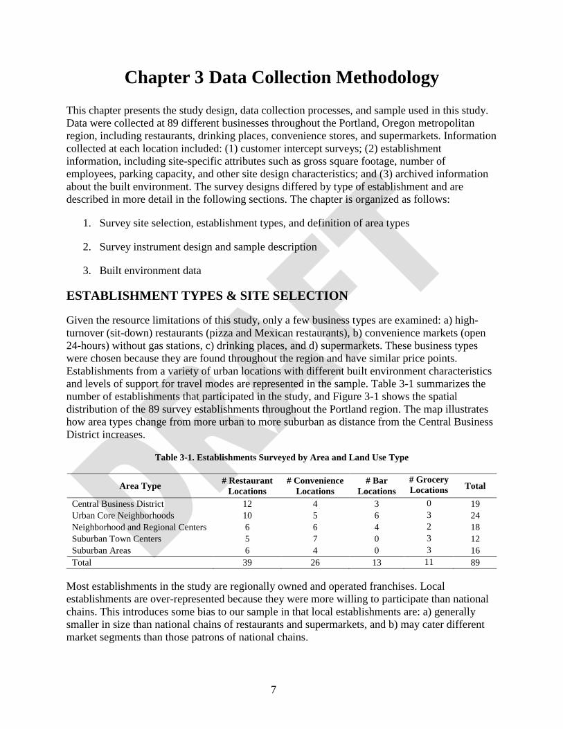
and levels of support for travel modes are represented in the sample. Table 3-1 summarizes the

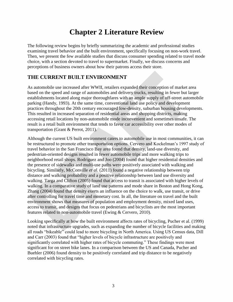
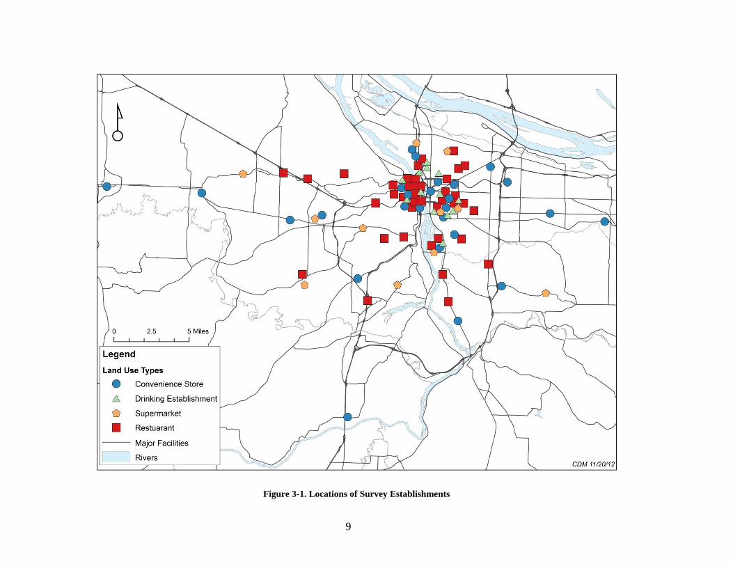
number of establishments that participated in the study, and Figure 3-1 shows the spatial

distribution of the 89 survey establishments throughout the Portland region. The map illustrates

how area types change from more urban to more suburban as distance from the Central Business

District increases.

Table 3-1. Establishments Surveyed by Area and Land Use Type

Area Type # Restaurant

Locations

# Convenience

Locations

# Bar

Locations

# Grocery

Locations Total

Central Business District 12 4 3 0 19

Urban Core Neighborhoods 10 5 6 3 24

Neighborhood and Regional Centers 6 6 4 2 18

Suburban Town Centers 5 7 0 3 12

Suburban Areas 6 4 0 3 16

Total 39 26 13 11 89

Most establishments in the study are regionally owned and operated franchises. Local

establishments are over-represented because they were more willing to participate than national

chains. This introduces some bias to our sample in that local establishments are: a) generally

smaller in size than national chains of restaurants and supermarkets, and b) may cater different

market segments than those patrons of national chains.

9

Figure 3-1. Locations of Survey Establishments

10

CUSTOMER SURVEYS

This section details the survey methodology. Two different survey designs were used for this

study: one for collecting information from customers at restaurants, drinking places and

convenience stores and another for supermarket patrons. These two surveys will be discussed

separately.

Restaurants, Drinking Establishments and Convenience Stores

Intercept surveys were administered by students as customers exited the establishments. Two

survey options were offered to patrons. First, a five-minute survey administered via handheld

computer tablets was offered. This survey instrument can be found in Appendix A. This “long

survey” collected information on: demographics of the respondent and his/her household, travel

mode(s), consumer spending behavior, frequency of trips to this establishment, attitudes towards

transportation modes, the trip to and from the establishment, and map locations of home, work,

trip origin and the following destination.

If a potential respondent refused the long survey, a short survey with four questions was offered

as an alternative. This survey instrument can be found in Appendix B. The short survey collected

information about: mode of travel, amount spent on that trip, frequency of visits to the

establishment, and the respondent’s home location. Gender was recorded by the survey

administrator.

Data were collected for restaurants, convenience stores and drinking places in 2011 from June

through early October. Because of the relatively small number of establishments surveyed, we

controlled for weather by only collecting data on days with favorable conditions. Data collection

occurred from 5:00PM to 7:00PM on Mondays, Tuesdays, Wednesdays, and Thursdays, as they

are considered “typical” travel days. The 5:00PM to 7:00PM time window was chosen to overlap

with the conventional weekday peak hour of automobile traffic (4:00PM to 6:00PM) as well as

the estimated peak hour of customer traffic for some land uses.1

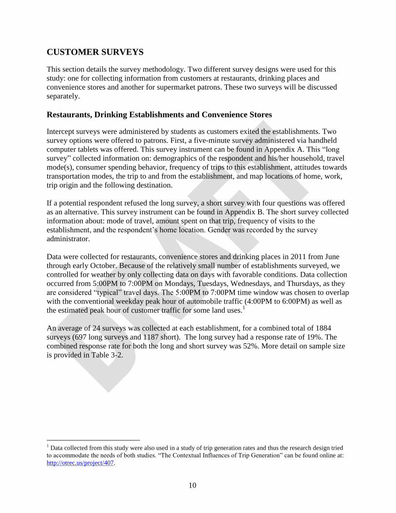
An average of 24 surveys was collected at each establishment, for a combined total of 1884

surveys (697 long surveys and 1187 short). The long survey had a response rate of 19%. The

combined response rate for both the long and short survey was 52%. More detail on sample size

is provided in Table 3-2.

1 Data collected from this study were also used in a study of trip generation rates and thus the research design tried

to accommodate the needs of both studies. “The Contextual Influences of Trip Generation” can be found online at:

http://otrec.us/project/407.

11

Table 3-2. Survey Sample Size

Response Rates

Land Use Establishments

(N)

Long

Surveys (N)

Short

Surveys (N)

Long

Survey

Short and

Long

Survey

Total

Drinking places 13 107 108 30% 50% 215

Convenience 26 281 710 14% 61% 991

Restaurants 39 309 369 24% 52% 678

Total 78 697 1187 19% 52% 1884

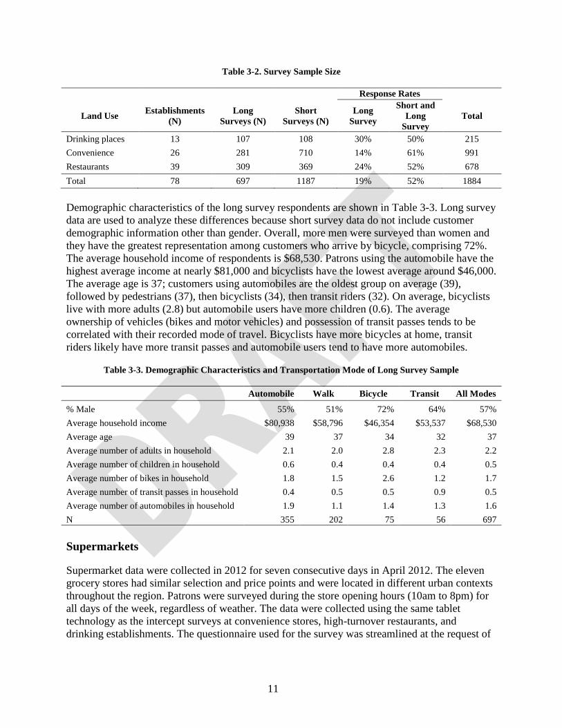
Demographic characteristics of the long survey respondents are shown in Table 3-3. Long survey

data are used to analyze these differences because short survey data do not include customer

demographic information other than gender. Overall, more men were surveyed than women and

they have the greatest representation among customers who arrive by bicycle, comprising 72%.

The average household income of respondents is $68,530. Patrons using the automobile have the

highest average income at nearly $81,000 and bicyclists have the lowest average around $46,000.

The average age is 37; customers using automobiles are the oldest group on average (39),

followed by pedestrians (37), then bicyclists (34), then transit riders (32). On average, bicyclists

live with more adults (2.8) but automobile users have more children (0.6). The average

ownership of vehicles (bikes and motor vehicles) and possession of transit passes tends to be

correlated with their recorded mode of travel. Bicyclists have more bicycles at home, transit

riders likely have more transit passes and automobile users tend to have more automobiles.

Table 3-3. Demographic Characteristics and Transportation Mode of Long Survey Sample

Automobile Walk Bicycle Transit All Modes

% Male 55% 51% 72% 64% 57%

Average household income $80,938 $58,796 $46,354 $53,537 $68,530

Average age 39 37 34 32 37

Average number of adults in household 2.1 2.0 2.8 2.3 2.2

Average number of children in household 0.6 0.4 0.4 0.4 0.5

Average number of bikes in household 1.8 1.5 2.6 1.2 1.7

Average number of transit passes in household 0.4 0.5 0.5 0.9 0.5

Average number of automobiles in household 1.9 1.1 1.4 1.3 1.6

N 355 202 75 56 697

Supermarkets

Supermarket data were collected in 2012 for seven consecutive days in April 2012. The eleven

grocery stores had similar selection and price points and were located in different urban contexts

throughout the region. Patrons were surveyed during the store opening hours (10am to 8pm) for

all days of the week, regardless of weather. The data were collected using the same tablet

technology as the intercept surveys at convenience stores, high-turnover restaurants, and

drinking establishments. The questionnaire used for the survey was streamlined at the request of

12

the management of the stores out of concern about customer burden and privacy (see Appendix

C for the survey instrument).

Store employees were provided a survey tablet with a survey application that was developed by

the Portland State University team. The survey was administered as customers were completing

their shopping transaction or leaving the store. The survey collected the following information:

Time of day

Date

Customer home location

Mode used to reach the store

Whether or not the customer was coming from home

Expenditures for that trip

Frequency of shopping at that store

Number of people the purchase was for (for that expenditure amount)

Gender

Each store obtained approximately 1,500 responses for a total of nearly 20,000 surveys. After

removing incomplete surveys, a total of 19,653 responses were eligible for analysis. Using the

total number of register transactions for each of the survey days, an approximate response rate

was calculated for each day and store location. The ratio of surveys collected to transactions

ranged from 6% to 12% for all supermarkets, with an average 10%.

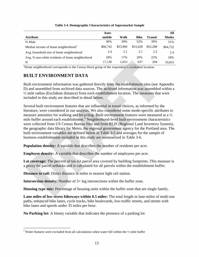
Characteristics and demographic information of the survey respondents are described below in

Table 3-4. This survey did not collect demographic information about the consumer or household

at the detailed level as the restaurant, bar and convenience store survey. To address this

limitation, data from the 2010 U.S. Census and 2009 American Community Survey (ACS) from

the block group were used to impute customer socio-economic information. The data from these

sources include: the median household income (ACS), the average household size (ACS), and

the percentage of people that are non-white (US Census). This imputation approach has

limitations in that it assumes customer characteristics can be represented by the average

characteristics of residents of their home neighborhoods.

Unlike the respondents surveyed at restaurants, bars and convenience stores, the supermarket

patrons surveyed were overwhelmingly women (69%) but similar to the other survey, men have

the greatest representation among customers who bicycle (52%). The sample lives in areas with

an average median income of around $68,000. Of those surveyed, customers who arrive by car

live in the highest median income neighborhoods on average and transit riders live in areas with

the lowest. Information about home neighborhood (Census block group) of respondents shows

that automobile patrons tend live in areas with more children per household and tend to live in

areas that are less diverse than patrons that use other modes.

13

Table 3-4. Demographic Characteristics of Supermarket Sample

Attribute

Auto-

mobile Walk Bike Transit

All

Modes

% Male 30% 39% 52% 39% 31%

Median income of home neighborhood1 $66,742 $53,960 $53,428 $52,288 $64,722

Avg. household size of home neighborhood 2.4 2.1 2.1 2.2 2.4

Avg. % non-white residents of home neighborhood 18% 17% 20% 22% 18%

N 17,130 1,653 637 204 19,653 1Home neighborhood corresponds to the Census block group of the respondent’s residential location.

BUILT ENVIRONMENT DATA

Built environment information was gathered directly from the establishment sites (see Appendix

D) and assembled from archived data sources. The archived information was assembled within a

½ mile radius (Euclidean distance) from each establishment location. The measures that were

included in this study are described in detail below.

Several built environment features that are influential in travel choices, as informed by the

literature, were considered in our analysis. We also considered some mode-specific attributes to

measure amenities for walking and bicycling. Built environment features were measured at a ½

mile buffer around each establishment.2 Neighborhood-level built environment characteristics

were collected from US Census Bureau files and from RLIS (Regional Land Inventory System),

the geographic data library for Metro, the regional government agency for the Portland area. The

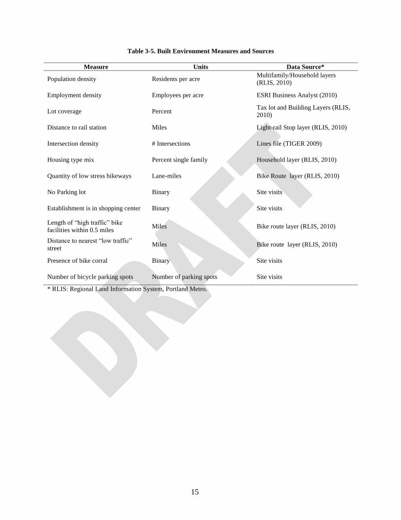
built environment variables are defined below in Table 3-5 and averages for the sample of

business establishments included in this study are summarized in Table 3-6.

Population density: A variable that describes the number of residents per acre.

Employee density: A variable that describes the number of employees per acre.

Lot coverage: The percent of tax-lot parcel area covered by building footprints. This measure is

a proxy for parcel setbacks and is calculated for all parcels within the establishment buffer.

Distance to rail: Direct distance in miles to nearest light rail station.

Intersection density: Number of 3+ leg intersections within the buffer zone.

Housing type mix: Percentage of housing units within the buffer zone that are single family.

Lane miles of low stress bikeways within 0.5 miles: The total length in lane-miles of multi-use

paths, enhanced bike lanes, cycle tracks, bike boulevards, low-traffic streets, and streets with

bike lanes and speeds under 35 miles per hour.

No Parking lot: A binary variable that indicates the presence of a parking lot.

2 Water features were excluded from all calculations when water fell within the ½ mile buffer

14

Establishment is in shopping center: A binary variable that indicates if an establishment is

located within a shopping center. Shopping centers as defined as strip mall-type developments

with at least three stores. These are different than urban shopping districts.

Distance to nearest “low traffic” street: The straight line distance to the nearest street with no

designated bikeway and posted speeds less than 25 miles per hour.

Length of “high traffic” bike facilities within 0.5 miles: The length in miles of roads with bike

lanes and posted speed limits greater than 35 miles per hour within 0.5 miles.

Presence of bike corral within 200ft of establishment: A bike corral typically has 6 to 12

bicycle racks in a row, often replaces on-street automobile parking and can park 10 to 20

bicycles. This uses space otherwise occupied by one to two cars. This variable is a binary

variable that indicates if the establishment has a bike corral within 200ft of the entrance.

Number of bicycle parking sports on site + adjacent street: A count of the number of bicycle

parking spots on the street immediately serving the establishment and the adjacent street. The

measure is calculated for the number of bicycles that could be parked, i.e. a bike parking staple

has two bike parking spots.

15

Table 3-5. Built Environment Measures and Sources

Measure Units Data Source*

Population density Residents per acre Multifamily/Household layers

(RLIS, 2010)

Employment density Employees per acre ESRI Business Analyst (2010)

Lot coverage Percent Tax lot and Building Layers (RLIS,

2010)

Distance to rail station Miles Light-rail Stop layer (RLIS, 2010)

Intersection density # Intersections Lines file (TIGER 2009)

Housing type mix Percent single family Household layer (RLIS, 2010)

Quantity of low stress bikeways Lane-miles Bike Route layer (RLIS, 2010)

No Parking lot Binary Site visits

Establishment is in shopping center Binary Site visits

Length of “high traffic” bike

facilities within 0.5 miles Miles Bike route layer (RLIS, 2010)

Distance to nearest “low traffic”

street Miles Bike route layer (RLIS, 2010)

Presence of bike corral Binary Site visits

Number of bicycle parking spots Number of parking spots Site visits

* RLIS: Regional Land Information System, Portland Metro.

16

Table 3-6. Average Site Characteristics of Establishments

Site attribute

Supermarket

N= 11

Convenience

Store

N = 26

Bar/Restaurant

N = 52

All

N = 89

Population density (people per acre) 7.9 11.9 14.7 13.0

Employee density (employees per acre) 3.4 16.0 23.3 18.7

Lot coverage (%) 19% 25% 30% 27%

Distance to rail (mi) 1.5 1.7 1.3 1.5

Intersection density (# intersections) 13.0 15.1 18.1 16.6

Housing type mix (% single family

detached) 55% 46% 43% 46%

Quantity of low stress bikeways (mi) 2.8 2.0 2.3 2.3

No parking lot 0% 4% 52% 32%

Establishment is in a shopping center 55% 12% 25% 25%

Length of “high traffic” bike facilities

within 0.5 miles .33 .27 .24 .26

Distance to nearest “low traffic” bike

facility(mi) 0.20 0.20 0.21 0.21

Presence of bike corral within 200’ 0% 12% 16% 13%

Bike parking spots 25 2.5 11 10

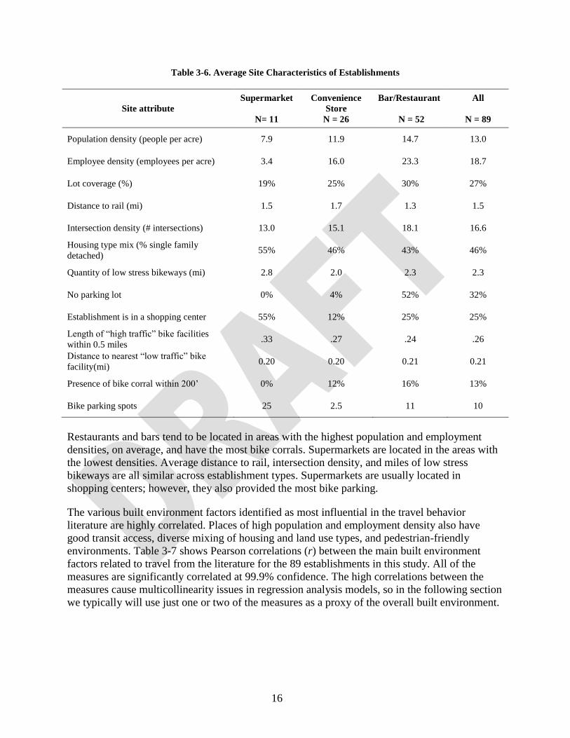
Restaurants and bars tend to be located in areas with the highest population and employment

densities, on average, and have the most bike corrals. Supermarkets are located in the areas with

the lowest densities. Average distance to rail, intersection density, and miles of low stress

bikeways are all similar across establishment types. Supermarkets are usually located in

shopping centers; however, they also provided the most bike parking.

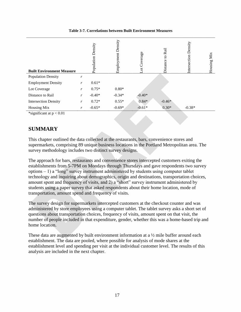
The various built environment factors identified as most influential in the travel behavior

literature are highly correlated. Places of high population and employment density also have

good transit access, diverse mixing of housing and land use types, and pedestrian-friendly

environments. Table 3-7 shows Pearson correlations (r) between the main built environment

factors related to travel from the literature for the 89 establishments in this study. All of the

measures are significantly correlated at 99.9% confidence. The high correlations between the

measures cause multicollinearity issues in regression analysis models, so in the following section

we typically will use just one or two of the measures as a proxy of the overall built environment.

17

Table 3-7. Correlations between Built Environment Measures

Built Environment Measure

Po

pu

lati

on

Den

sity

Em

plo

ym

ent

Den

sity

Lo

t C

ov

erag

e

Dis

tan

ce t

o R

ail

Inte

rsec

tio

n D

ensi

ty

Ho

usi

ng

Mix

Population Density r

Employment Density r 0.61 *

Lot Coverage r 0.75 * 0.80 *

Distance to Rail r -0.40 * -0.34 * -0.40 *

Intersection Density r 0.72 * 0.55 * 0.84 * -0.46 *

Housing Mix r -0.65 * -0.69 * -0.61 * 0.30 * -0.38 *

*significant at p < 0.01

SUMMARY

This chapter outlined the data collected at the restaurants, bars, convenience stores and

supermarkets, comprising 89 unique business locations in the Portland Metropolitan area. The

survey methodology includes two distinct survey designs.

The approach for bars, restaurants and convenience stores intercepted customers exiting the

establishments from 5-7PM on Mondays through Thursdays and gave respondents two survey

options – 1) a “long” survey instrument administered by students using computer tablet

technology and inquiring about demographics, origin and destinations, transportation choices,

amount spent and frequency of visits, and 2) a “short” survey instrument administered by

students using a paper survey that asked respondents about their home location, mode of

transportation, amount spend and frequency of visits.

The survey design for supermarkets intercepted customers at the checkout counter and was

administered by store employees using a computer tablet. The tablet survey asks a short set of

questions about transportation choices, frequency of visits, amount spent on that visit, the

number of people included in that expenditure, gender, whether this was a home-based trip and

home location.

These data are augmented by built environment information at a ½ mile buffer around each

establishment. The data are pooled, where possible for analysis of mode shares at the

establishment level and spending per visit at the individual customer level. The results of this

analysis are included in the next chapter.

18

Analysis and Results Chapter 4

In this chapter, the data are analyzed to understand the connections between mode of travel,

frequency of trips, and spending at restaurants, bars, convenience stores, and supermarkets. In

the first section, summary statistics are reported. Here, the analysis considers only a few

elements and often presents averages. It is important to examine and control for the various

characteristics and conditions that contribute to the consumer behaviors and mode choices of

interest. As such, the second section presents the results of multivariate models that help better

interpret and explain the relationships between the various choices and associated factors. The

first set of models estimates mode shares of bicyclists and non-automobile travelers at the

establishment level, and the second set estimates spending per trip at the individual level for

different establishment types.

SUMMARY STATISTICS

This section details observed travel behavior and consumer spending data from customers at

establishments described in the previous chapter. We describe differences between travelers,

mode shares, trip lengths, trip frequencies, and spending behavior by establishment type. Unless

otherwise noted, the supermarket data reported in this section refer to the entire seven day,

10AM – 8PM sample; reported data from convenience stores, drinking establishments, and high-

turnover restaurants refer to the Monday through Thursday 5PM – 7PM sample.

Mode Shares

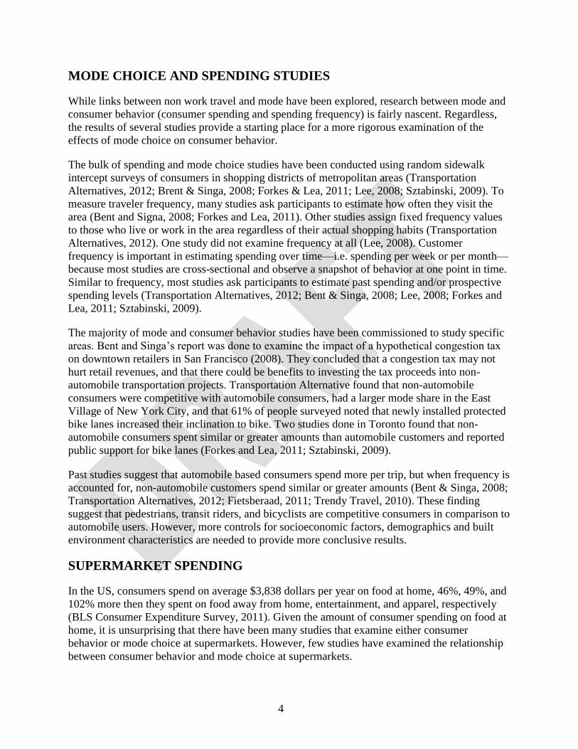
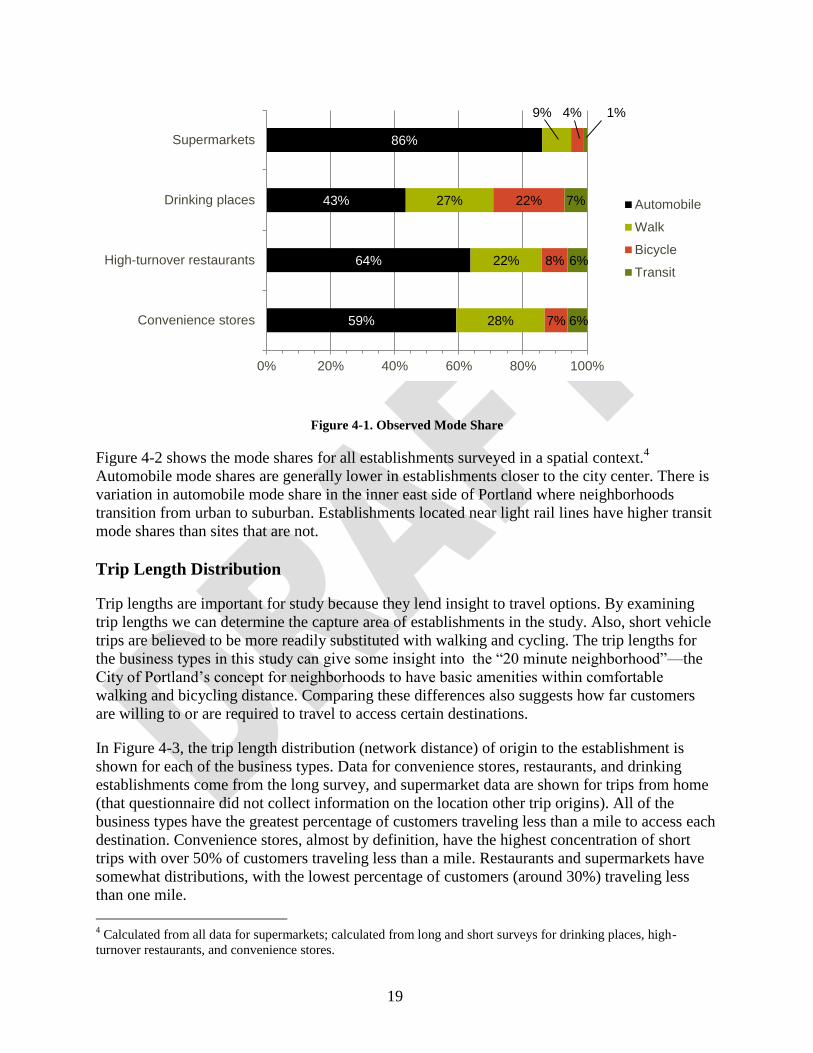
Figure 4-1 shows the observed mode shares3 by each establishment type. The automobile is

clearly the dominant mode for customers across all establishments and transit is the least used

mode.

Supermarkets see the most use of the automobile, with 86% of trips made by private vehicle.

This is likely due to the nature of grocery shopping: stores are typically located on arterial

streets, shoppers purchase goods they have to transport, and the volume of goods purchased is

typically greater than at convenience stores, restaurants, and drinking places. Drinking places

have the lowest automobile mode share of the four business types surveyed. Only 43% of patrons

arrive by automobile.

Of the non-automobile modes, walking has the highest mode share across land uses. Walking

rates are highest for convenience stores and drinking places, both with 27% mode share.

Restaurants have a 22% walk mode share and supermarkets have 9% of patrons as pedestrians.

Bicycling is most popular at drinking establishments, where 22% of patrons arrive by bike.

Restaurants, convenience stores, and supermarkets have 8%, 7%, and 4% bike mode share,

respectively. Transit use is fairly consistent across convenience stores (6%), restaurants (6%) and

drinking places (7%), but only 1% of shoppers at supermarkets arrived by transit.

3 Calculated from all data for supermarkets; calculated from long and short surveys for drinking places, high-

turnover restaurants, and convenience stores.

19

Figure 4-1. Observed Mode Share

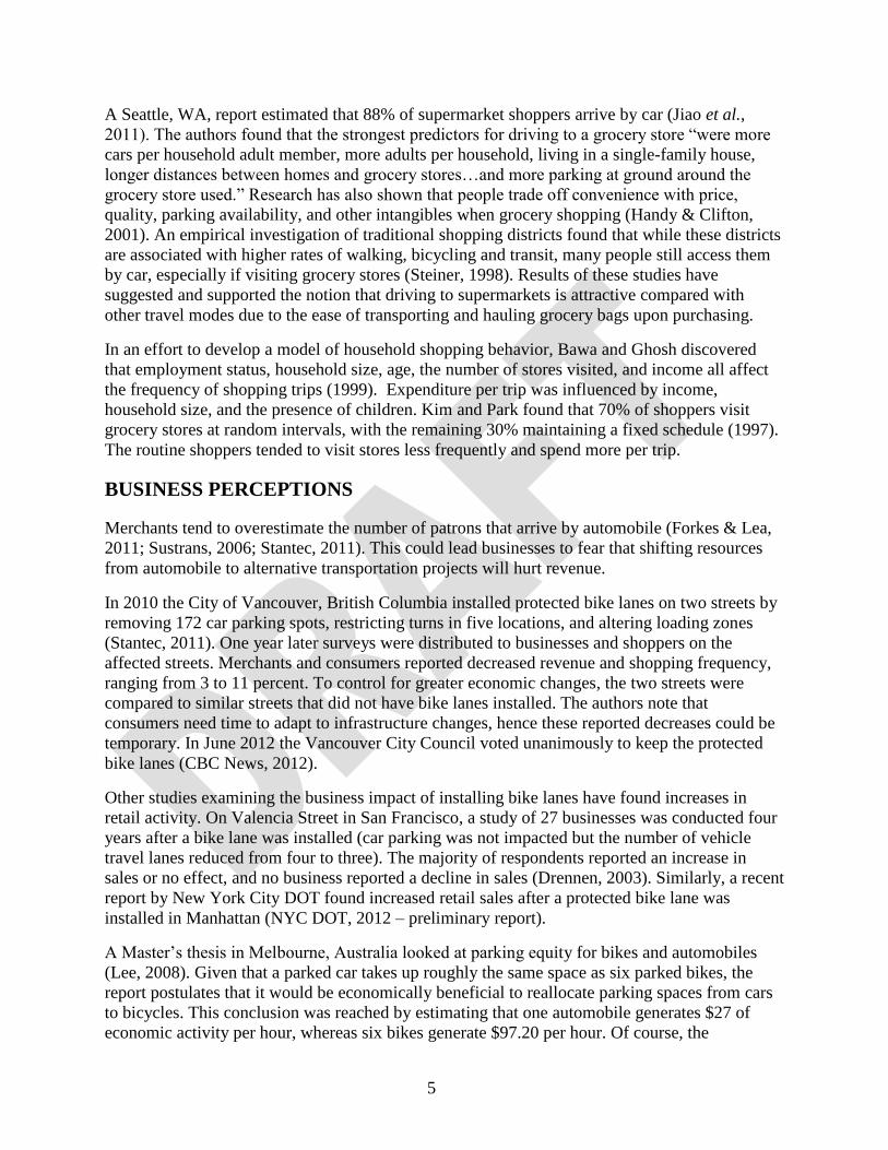
Figure 4-2 shows the mode shares for all establishments surveyed in a spatial context.4

Automobile mode shares are generally lower in establishments closer to the city center. There is

variation in automobile mode share in the inner east side of Portland where neighborhoods

transition from urban to suburban. Establishments located near light rail lines have higher transit

mode shares than sites that are not.

Trip Length Distribution

Trip lengths are important for study because they lend insight to travel options. By examining

trip lengths we can determine the capture area of establishments in the study. Also, short vehicle

trips are believed to be more readily substituted with walking and cycling. The trip lengths for

the business types in this study can give some insight into the “20 minute neighborhood”—the

City of Portland’s concept for neighborhoods to have basic amenities within comfortable

walking and bicycling distance. Comparing these differences also suggests how far customers

are willing to or are required to travel to access certain destinations.

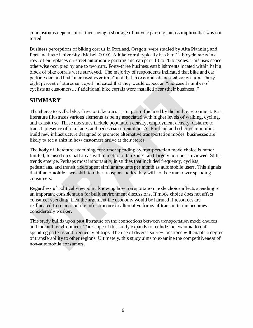
In Figure 4-3, the trip length distribution (network distance) of origin to the establishment is

shown for each of the business types. Data for convenience stores, restaurants, and drinking

establishments come from the long survey, and supermarket data are shown for trips from home

(that questionnaire did not collect information on the location other trip origins). All of the

business types have the greatest percentage of customers traveling less than a mile to access each

destination. Convenience stores, almost by definition, have the highest concentration of short

trips with over 50% of customers traveling less than a mile. Restaurants and supermarkets have

somewhat distributions, with the lowest percentage of customers (around 30%) traveling less

than one mile.

4 Calculated from all data for supermarkets; calculated from long and short surveys for drinking places, high-

turnover restaurants, and convenience stores.

59%

64%

43%

86%

28%

22%

27%

9%

7%

8%

22%

4%

6%

6%

7%

1%

0% 20% 40% 60% 80% 100%

Convenience stores

High-turnover restaurants

Drinking places

Supermarkets

Automobile

Walk

Bicycle

Transit

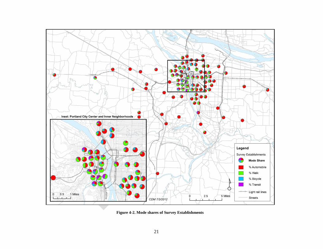
21

Figure 4-2. Mode shares of Survey Establishments

22

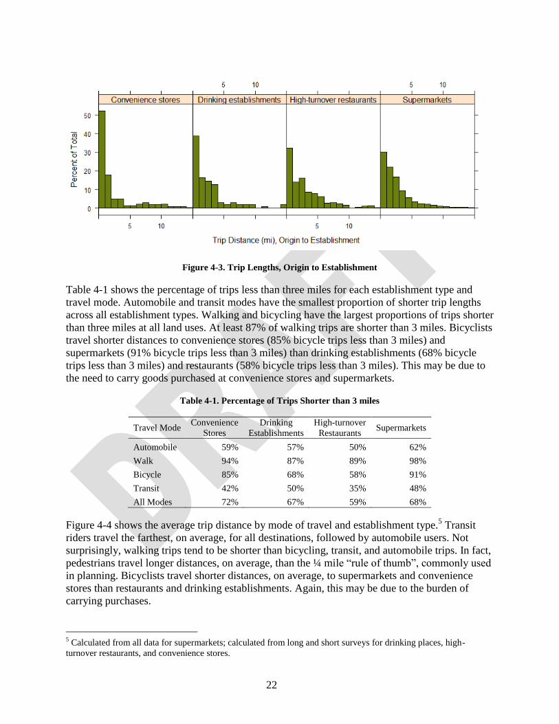
Figure 4-3. Trip Lengths, Origin to Establishment

Table 4-1 shows the percentage of trips less than three miles for each establishment type and

travel mode. Automobile and transit modes have the smallest proportion of shorter trip lengths

across all establishment types. Walking and bicycling have the largest proportions of trips shorter

than three miles at all land uses. At least 87% of walking trips are shorter than 3 miles. Bicyclists

travel shorter distances to convenience stores (85% bicycle trips less than 3 miles) and

supermarkets (91% bicycle trips less than 3 miles) than drinking establishments (68% bicycle

trips less than 3 miles) and restaurants (58% bicycle trips less than 3 miles). This may be due to

the need to carry goods purchased at convenience stores and supermarkets.

Table 4-1. Percentage of Trips Shorter than 3 miles

Travel Mode Convenience

Stores

Drinking

Establishments

High-turnover

Restaurants Supermarkets

Automobile 59% 57% 50% 62%

Walk 94% 87% 89% 98%

Bicycle 85% 68% 58% 91%

Transit 42% 50% 35% 48%

All Modes 72% 67% 59% 68%

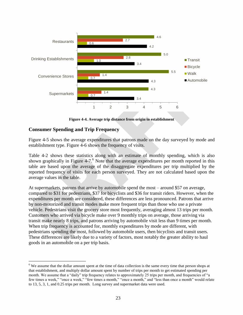
Figure 4-4 shows the average trip distance by mode of travel and establishment type.5 Transit

riders travel the farthest, on average, for all destinations, followed by automobile users. Not

surprisingly, walking trips tend to be shorter than bicycling, transit, and automobile trips. In fact,

pedestrians travel longer distances, on average, than the ¼ mile “rule of thumb”, commonly used

in planning. Bicyclists travel shorter distances, on average, to supermarkets and convenience

stores than restaurants and drinking establishments. Again, this may be due to the burden of

carrying purchases.

5 Calculated from all data for supermarkets; calculated from long and short surveys for drinking places, high-

turnover restaurants, and convenience stores.

23

Figure 4-4. Average trip distance from origin to establishment

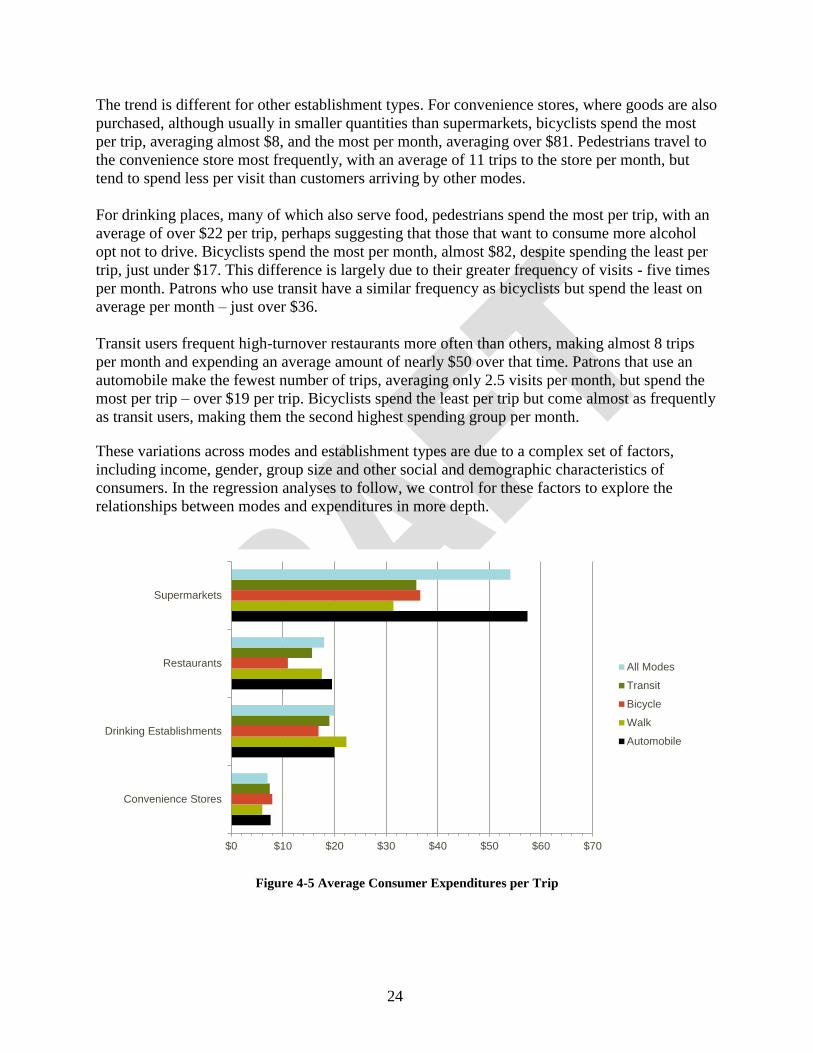
Consumer Spending and Trip Frequency

Figure 4-5 shows the average expenditures that patrons made on the day surveyed by mode and

establishment type. Figure 4-6 shows the frequency of visits.

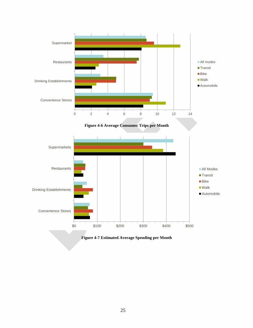
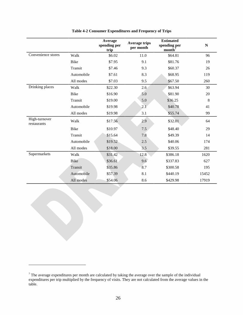
Table 4-2 shows these statistics along with an estimate of monthly spending, which is also

shown graphically in Figure 4-7.6 Note that the average expenditures per month reported in this

table are based upon the average of the disaggregate expenditures per trip multiplied by the

reported frequency of visits for each person surveyed. They are not calculated based upon the

average values in the table.

At supermarkets, patrons that arrive by automobile spend the most – around $57 on average,

compared to $31 for pedestrians, $37 for bicyclists and $36 for transit riders. However, when the

expenditures per month are considered, these differences are less pronounced. Patrons that arrive

by non-motorized and transit modes make more frequent trips than those who use a private

vehicle. Pedestrians visit the grocery store most frequently, averaging almost 13 trips per month.

Customers who arrived via bicycle make over 9 monthly trips on average, those arriving via

transit make nearly 8 trips, and patrons arriving by automobile visit less than 9 times per month.

When trip frequency is accounted for, monthly expenditures by mode are different, with

pedestrians spending the most, followed by automobile users, then bicyclists and transit users.

These differences are likely due to a variety of factors, most notably the greater ability to haul

goods in an automobile on a per trip basis.

6 We assume that the dollar amount spent at the time of data collection is the same every time that person shops at

that establishment, and multiply dollar amount spent by number of trips per month to get estimated spending per

month. We assume that a “daily” trip frequency relates to approximately 25 trips per month, and frequencies of “a

few times a week,” “once a week,” “few times a month,” “once a month,” and “less than once a month” would relate

to 13, 5, 3, 1, and 0.25 trips per month. Long survey and supermarket data were used.

3.4

4.3

3.4

4.2

0.7

0.7

1.0

0.6

1.4

1.4

2.8

2.7

4.3

5.5

5.0

4.6

1 2 3 4 5 6

Supermarkets

Convenience Stores

Drinking Establishments

Restaurants

Transit

Bicycle

Walk

Automobile

24

The trend is different for other establishment types. For convenience stores, where goods are also

purchased, although usually in smaller quantities than supermarkets, bicyclists spend the most

per trip, averaging almost $8, and the most per month, averaging over $81. Pedestrians travel to

the convenience store most frequently, with an average of 11 trips to the store per month, but

tend to spend less per visit than customers arriving by other modes.

For drinking places, many of which also serve food, pedestrians spend the most per trip, with an

average of over $22 per trip, perhaps suggesting that those that want to consume more alcohol

opt not to drive. Bicyclists spend the most per month, almost $82, despite spending the least per

trip, just under $17. This difference is largely due to their greater frequency of visits - five times

per month. Patrons who use transit have a similar frequency as bicyclists but spend the least on

average per month – just over $36.

Transit users frequent high-turnover restaurants more often than others, making almost 8 trips

per month and expending an average amount of nearly $50 over that time. Patrons that use an

automobile make the fewest number of trips, averaging only 2.5 visits per month, but spend the

most per trip – over $19 per trip. Bicyclists spend the least per trip but come almost as frequently

as transit users, making them the second highest spending group per month.

These variations across modes and establishment types are due to a complex set of factors,

including income, gender, group size and other social and demographic characteristics of

consumers. In the regression analyses to follow, we control for these factors to explore the

relationships between modes and expenditures in more depth.

Figure 4-5 Average Consumer Expenditures per Trip

$0 $10 $20 $30 $40 $50 $60 $70

Convenience Stores

Drinking Establishments

Restaurants

Supermarkets

All Modes

Transit

Bicycle

Walk

Automobile

25

Figure 4-6 Average Consumer Trips per Month

Figure 4-7 Estimated Average Spending per Month

0 2 4 6 8 10 12 14

Convenience Stores

Drinking Establishments

Restaurants

Supermarket

All modes

Transit

Bike

Walk

Automobile

$0 $100 $200 $300 $400 $500

Convenience Stores

Drinking Establishments

Restaurants

Supermarkets

All Modes

Transit

Bike

Walk

Automobile

26

Table 4-2 Consumer Expenditures and Frequency of Trips

Average

spending per

trip

Average trips

per month

Estimated

spending per

month7

N

Convenience stores Walk $6.02 11.0 $64.81 96

Bike $7.95 9.1 $81.76 19

Transit $7.46 9.3 $60.37 26

Automobile $7.61 8.3 $68.95 119

All modes $7.03 9.5 $67.50 260

Drinking places Walk $22.30 2.6 $63.94 30

Bike $16.90 5.0 $81.90 20

Transit $19.00 5.0 $36.25 8

Automobile $19.98 2.1 $40.78 41

All modes $19.98 3.1 $55.74 99

High-turnover

restaurants Walk $17.56 2.9 $32.01 64

Bike $10.97 7.5 $48.40 29

Transit $15.64 7.8 $49.39 14

Automobile $19.52 2.5 $40.06 174

All modes $18.00 3.5 $39.55 281

Supermarkets Walk $31.42 12.8 $386.18 1620

Bike $36.61 9.6 $337.83 627

Transit $35.86 8.7 $300.58 195

Automobile $57.39 8.1 $440.19 15452

All modes $54.06 8.6 $429.98 17919

7 The average expenditures per month are calculated by taking the average over the sample of the individual

expenditures per trip multiplied by the frequency of visits. They are not calculated from the average values in the

table.

27

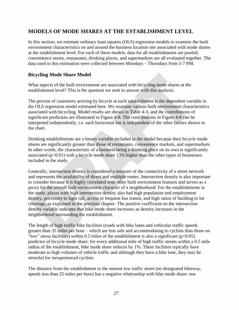
MODELS OF MODE SHARES AT THE ESTABLISHMENT LEVEL

In this section, we estimate ordinary least squares (OLS) regression models to examine the built

environment characteristics on and around the business location site associated with mode shares

at the establishment level. For each of these models, data for all establishments are pooled;

convenience stores, restaurants, drinking places, and supermarkets are all evaluated together. The

data used in this estimation were collected between Mondays – Thursdays from 5-7 PM.

Bicycling Mode Share Model

What aspects of the built environment are associated with bicycling mode shares at the

establishment level? This is the question we seek to answer with this analysis.

The percent of customers arriving by bicycle at each establishment is the dependent variable in

the OLS regression model estimated here. We examine various built environment characteristics

associated with bicycling. Model results are shown in Table 4-3, and the contributions of

significant predictors are illustrated in Figure 4-8. The contributions in Figure 4-8 can be

interpreted independently, i.e. each horizontal bar is independent of the other factors shown in

the chart.

Drinking establishments are a binary variable included in the model because their bicycle mode

shares are significantly greater than those of restaurants, convenience markets, and supermarkets.

In other words, the characteristic of a business being a drinking place on its own is significantly

associated (p<0.01) with a bicycle mode share 13% higher than the other types of businesses

included in the study.

Generally, intersection density is considered a measure of the connectivity of a street network

and represents the availability of direct and multiple routes. Intersection density is also important

to consider because it is highly correlated with other built environment features and serves as a

proxy for the overall built environment character of a neighborhood. For the establishments in

the study, places with high intersection density also had high population and employment

density, proximity to light rail, access to frequent bus transit, and high ratios of building to lot

coverage, as explained in the previous chapter. The positive coefficient on the intersection

density variable indicates that bike mode share increases as density increases in the

neighborhood surrounding the establishment.

The length of high traffic bike facilities (roads with bike lanes and vehicular traffic speeds

greater than 35 miles per hour – which are less safe and accommodating to cyclists than those on

“low” stress facilities) within 0.5 miles of the establishment is also a significant (p<0.05)

predictor of bicycle mode share: for every additional mile of high traffic streets within a 0.5 mile

radius of the establishment, bike mode share reduces by 1%. These facilities typically have

moderate to high volumes of vehicle traffic and although they have a bike lane, they may be

stressful for inexperienced cyclists.

The distance from the establishment to the nearest low traffic street (no designated bikeway,

speeds less than 25 miles per hour) has a negative relationship with bike mode share: one

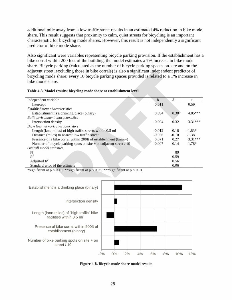
28

additional mile away from a low traffic street results in an estimated 4% reduction in bike mode

share. This result suggests that proximity to calm, quiet streets for bicycling is an important

characteristic for bicycling mode shares. However, this result is not independently a significant

predictor of bike mode share.

Also significant were variables representing bicycle parking provision. If the establishment has a

bike corral within 200 feet of the building, the model estimates a 7% increase in bike mode

share. Bicycle parking (calculated as the number of bicycle parking spaces on-site and on the

adjacent street, excluding those in bike corrals) is also a significant independent predictor of

bicycling mode share: every 10 bicycle parking spaces provided is related to a 1% increase in

bike mode share.

Table 4-3. Model results: bicycling mode share at establishment level

Independent variable b ß t

Intercept 0.011 0.59

Establishment characteristics

Establishment is a drinking place (binary) 0.094 0.38 4.85 ***

Built environment characteristics

Intersection density 0.004 0.32 3.31 ***

Bicycling network characteristics

Length (lane-miles) of high traffic streets within 0.5 mi -0.012 -0.16 -1.83 *

Distance (miles) to nearest low traffic street -0.036 -0.10 -1.38

Presence of a bike corral within 200ft of establishment (binary) 0.071 0.27 3.31 ***

Number of bicycle parking spots on site + on adjacent street / 10 0.007 0.14 1.78 *

Overall model statistics

N 89

R2 0.59

Adjusted R2 0.56

Standard error of the estimate 0.06

*significant at p < 0.10; **significant at p < 0.05; ***significant at p < 0.01

Figure 4-8. Bicycle mode share model results

-2% 0% 2% 4% 6% 8% 10% 12%

Number of bike parking spots on site + onstreet / 10

Presence of bike corral within 200ft ofestablishment (binary)

Length (lane-miles) of "high traffic" bikefacilities within 0.5 mi

Intersection density

Establishment is a drinking place (binary)

29

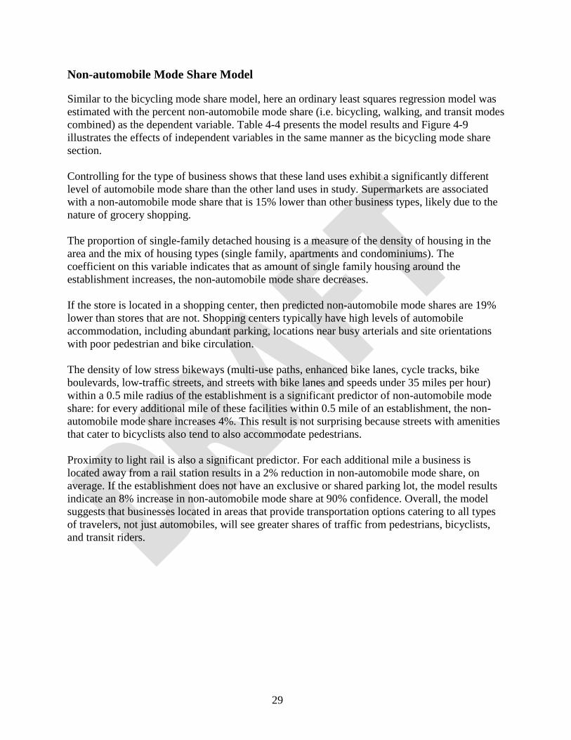
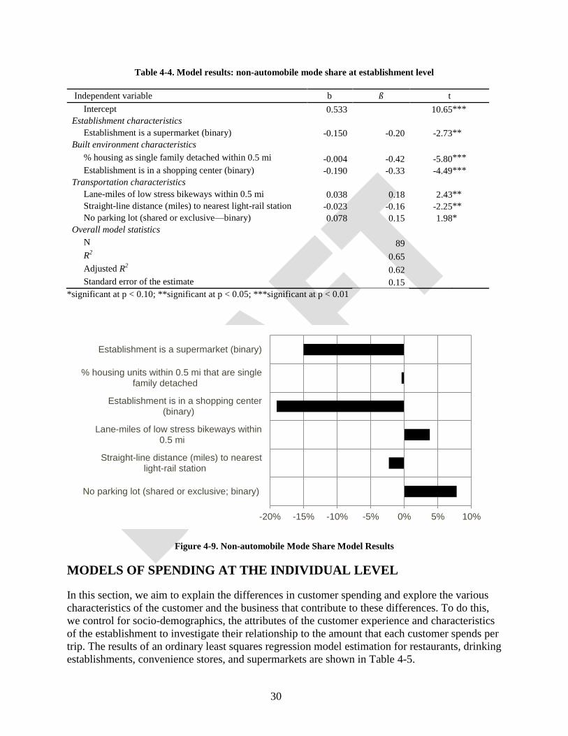
Non-automobile Mode Share Model

Similar to the bicycling mode share model, here an ordinary least squares regression model was

estimated with the percent non-automobile mode share (i.e. bicycling, walking, and transit modes

combined) as the dependent variable. Table 4-4 presents the model results and Figure 4-9

illustrates the effects of independent variables in the same manner as the bicycling mode share

section.

Controlling for the type of business shows that these land uses exhibit a significantly different

level of automobile mode share than the other land uses in study. Supermarkets are associated

with a non-automobile mode share that is 15% lower than other business types, likely due to the

nature of grocery shopping.

The proportion of single-family detached housing is a measure of the density of housing in the

area and the mix of housing types (single family, apartments and condominiums). The

coefficient on this variable indicates that as amount of single family housing around the

establishment increases, the non-automobile mode share decreases.

If the store is located in a shopping center, then predicted non-automobile mode shares are 19%

lower than stores that are not. Shopping centers typically have high levels of automobile

accommodation, including abundant parking, locations near busy arterials and site orientations

with poor pedestrian and bike circulation.

The density of low stress bikeways (multi-use paths, enhanced bike lanes, cycle tracks, bike

boulevards, low-traffic streets, and streets with bike lanes and speeds under 35 miles per hour)

within a 0.5 mile radius of the establishment is a significant predictor of non-automobile mode

share: for every additional mile of these facilities within 0.5 mile of an establishment, the non-

automobile mode share increases 4%. This result is not surprising because streets with amenities

that cater to bicyclists also tend to also accommodate pedestrians.

Proximity to light rail is also a significant predictor. For each additional mile a business is

located away from a rail station results in a 2% reduction in non-automobile mode share, on

average. If the establishment does not have an exclusive or shared parking lot, the model results

indicate an 8% increase in non-automobile mode share at 90% confidence. Overall, the model

suggests that businesses located in areas that provide transportation options catering to all types

of travelers, not just automobiles, will see greater shares of traffic from pedestrians, bicyclists,

and transit riders.

30

Table 4-4. Model results: non-automobile mode share at establishment level

Independent variable b ß t

Intercept 0.533

10.65 ***

Establishment characteristics

Establishment is a supermarket (binary) -0.150 -0.20 -2.73 **

Built environment characteristics

% housing as single family detached within 0.5 mi -0.004 -0.42 -5.80 ***

Establishment is in a shopping center (binary) -0.190 -0.33 -4.49 ***

Transportation characteristics

Lane-miles of low stress bikeways within 0.5 mi 0.038 0.18 2.43 **

Straight-line distance (miles) to nearest light-rail station -0.023 -0.16 -2.25 **

No parking lot (shared or exclusive—binary) 0.078 0.15 1.98 *

Overall model statistics

N 89

R2

0.65

Adjusted R2

0.62

Standard error of the estimate 0.15

*significant at p < 0.10; **significant at p < 0.05; ***significant at p < 0.01

Figure 4-9. Non-automobile Mode Share Model Results

MODELS OF SPENDING AT THE INDIVIDUAL LEVEL

In this section, we aim to explain the differences in customer spending and explore the various

characteristics of the customer and the business that contribute to these differences. To do this,

we control for socio-demographics, the attributes of the customer experience and characteristics

of the establishment to investigate their relationship to the amount that each customer spends per

trip. The results of an ordinary least squares regression model estimation for restaurants, drinking

establishments, convenience stores, and supermarkets are shown in Table 4-5.

-20% -15% -10% -5% 0% 5% 10%

No parking lot (shared or exclusive; binary)

Straight-line distance (miles) to nearestlight-rail station

Lane-miles of low stress bikeways within0.5 mi

Establishment is in a shopping center(binary)

% housing units within 0.5 mi that are singlefamily detached

Establishment is a supermarket (binary)

31

The dependent variable for the estimations is the log transform of spending per trip for each

customer. The customer spending is log-transformed8 to better fit a normal distribution. Because

of this transformation, the coefficients for independent variables are not easy to interpret. Thus

we interpret the unstandardized regression coefficient of a particular independent variable

(represented by B) as the predicted impact on amount spent per trip in percent, S, given by:

(1)

where ∆x is the change in the independent variable. This interpretation provides the sensitivity of

money spent per trip to an incremental change in any independent variable. In discussion, we

consider a unit change of one. Binary variables are interpreted by comparing to the base case.

The base case for each of the binary variables is: gender = female; age = under 25; no children in

the household; mode = automobile; trip frequency = “less than once per month”; restaurant type

= pizza or bar (restaurant and bar model only); purchase time of day = afternoon (supermarket

model only); purchase day = weekday (supermarket model only); store = store #8 (supermarket

model only).

Spending per Trip at Restaurants and Drinking Establishments

We consider the consumer and travel behavior for restaurants and drinking establishments

together because of the similarities in the nature of activities at these locations. Many of the

drinking places also sell food and many of the restaurants sell drinks. The goods purchased are

most commonly consumed on site. Thus, non-automobile modes are not disadvantaged by the

lack of carrying capacity. Combining these land uses is confirmed statistically by an analysis of

variance that showed average spending per trip was not significantly different between

restaurants and drinking establishments.9

The model for restaurants and drinking establishments yields the following set of significant

explanatory variables: presence of children in the household, household income, time spent in

the establishment, the group size, and whether the establishment is a Mexican restaurant. Survey

respondents report spending amounts anywhere from $2 to $150 at restaurants and bars.10

The

effects of the individual coefficients on amount spent are illustrated in Figure 4-10.

In terms of customer demographics, the presence of children in a patron’s household has a

significant impact on how much they spend: people with children spend an estimated 13.3% less

than those without. Household income was also a significant predictor of spending per trip, but

the impact was relatively small – for every additional $10,000 in household income, respondents

are expected to spend an estimated additional 1.6% at the establishment. Respondent gender,

age, and household size are included in estimation but are not significantly associated with

spending.

In terms of travel, no particular mode is significantly associated with spending, meaning that the

patron’s mode of transportation does not influence the amount spent once we control for other

8 A logarithmic transform with a base of 10 was used.

9 F(1,380) = 1.40, p-value = 0.237

10 The 25 customers who spent either zero or over 150 dollars were excluded from analysis.

32

factors. Trip distance is also not a factor, and neither are the interactions between trip modes and

distances. This result suggests that regardless of travel modes or distances, pedestrians,

bicyclists, transit riders, and automobile users all spend similar amounts per trip on average, all

else equal.

The variable with the greatest impact on restaurant expenditures is group size. Each additional

person in a group is associated with a 59% increase in spending, on average. The amount of time

spent at the establishment is also an independent predictor of spending – each minute in a

restaurant or bar is associated with a 1% increase on the bill.

Travel frequency differences from the “less than once per month” category are not significant

predictors of spending at restaurants and bars, but the signs and magnitudes of the coefficients

for frequent travelers (visits a few times per week and visits daily) indicate reduced spending for

each visit by regular customers compared to infrequent customers. Respondents spend an

average of 15.6% more at Mexican restaurants than at pizza restaurants and drinking

establishments.

Spending per Trip at Convenience Markets

The model of consumer spending per trip for convenience stores follows the same specification

with the exception of a binary variable for Mexican restaurants. The set of significant

explanatory variables includes: gender, age, the number of adults in the household, the time

spent in the establishment, group size, and the travel frequency. Respondents with spending

amounts between $1 and $50 at convenience stores were included in the analysis.11

The effects

of a unit increase in each of the significant variables on amount spent are illustrated in Figure

4-11.

In terms of customer demographics, respondent gender is a significant predictor of spending:

women spend an estimated 18.5% more in convenience markets than men. Also, customers

between 25-34 years old spend 38% more than patrons of other ages. The number of adults in the

household is associated with more spending, on average – 9.6% more is spent for every

additional adult. Unlike the spending model at restaurants and bars, household income and

presence of children are not significant predictors of spending at convenience stores.

Like the spending model at restaurants and bars, no trip characteristics—travel modes, distances,

and interactions of the two—are significantly related to spending per trip. This again suggests

that all customers spend similar amounts per trip at convenience stores regardless of their travel

mode or trip distance. Surprisingly, this indicates that the need to carry items purchased at

convenience stores does not translate into lower spending amounts for non-automobile travelers.

Perhaps the generally small quantity of goods purchased at these stores is not enough to have an

effect.

Like the spending at restaurants and bars model, the amount of time spent at the establishment is

an important indicator of spending – each minute spent in the store yields an additional 3.5%

11

The13 respondents who spent either zero or more than 50 dollars were considered outliers and were not included

in the analysis.

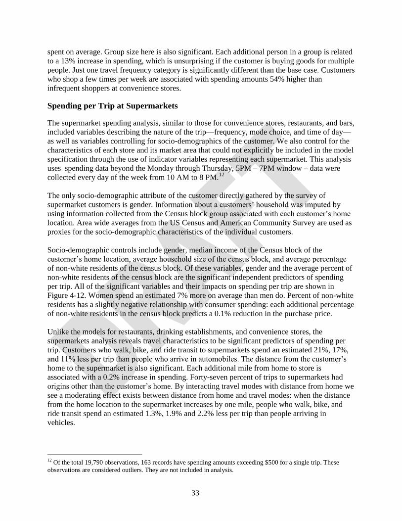
33

spent on average. Group size here is also significant. Each additional person in a group is related

to a 13% increase in spending, which is unsurprising if the customer is buying goods for multiple

people. Just one travel frequency category is significantly different than the base case. Customers

who shop a few times per week are associated with spending amounts 54% higher than

infrequent shoppers at convenience stores.

Spending per Trip at Supermarkets

The supermarket spending analysis, similar to those for convenience stores, restaurants, and bars,

included variables describing the nature of the trip—frequency, mode choice, and time of day—

as well as variables controlling for socio-demographics of the customer. We also control for the

characteristics of each store and its market area that could not explicitly be included in the model

specification through the use of indicator variables representing each supermarket. This analysis

uses spending data beyond the Monday through Thursday, 5PM – 7PM window – data were

collected every day of the week from 10 AM to 8 PM.12

The only socio-demographic attribute of the customer directly gathered by the survey of

supermarket customers is gender. Information about a customers’ household was imputed by

using information collected from the Census block group associated with each customer’s home

location. Area wide averages from the US Census and American Community Survey are used as

proxies for the socio-demographic characteristics of the individual customers.

Socio-demographic controls include gender, median income of the Census block of the

customer’s home location, average household size of the census block, and average percentage

of non-white residents of the census block. Of these variables, gender and the average percent of

non-white residents of the census block are the significant independent predictors of spending

per trip. All of the significant variables and their impacts on spending per trip are shown in

Figure 4-12. Women spend an estimated 7% more on average than men do. Percent of non-white

residents has a slightly negative relationship with consumer spending: each additional percentage

of non-white residents in the census block predicts a 0.1% reduction in the purchase price.

Unlike the models for restaurants, drinking establishments, and convenience stores, the

supermarkets analysis reveals travel characteristics to be significant predictors of spending per

trip. Customers who walk, bike, and ride transit to supermarkets spend an estimated 21%, 17%,

and 11% less per trip than people who arrive in automobiles. The distance from the customer’s

home to the supermarket is also significant. Each additional mile from home to store is

associated with a 0.2% increase in spending. Forty-seven percent of trips to supermarkets had

origins other than the customer’s home. By interacting travel modes with distance from home we

see a moderating effect exists between distance from home and travel modes: when the distance

from the home location to the supermarket increases by one mile, people who walk, bike, and

ride transit spend an estimated 1.3%, 1.9% and 2.2% less per trip than people arriving in

vehicles.

12

Of the total 19,790 observations, 163 records have spending amounts exceeding $500 for a single trip. These

observations are considered outliers. They are not included in analysis.

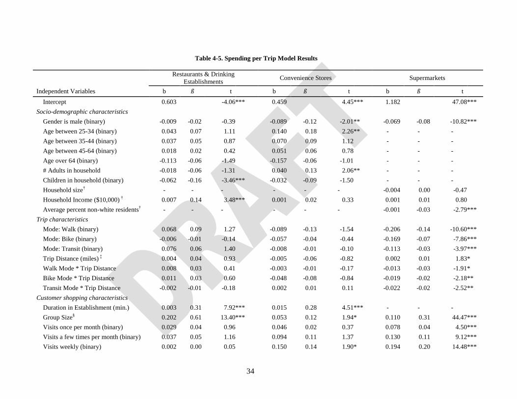
34

Table 4-5. Spending per Trip Model Results

Restaurants & Drinking

Establishments Convenience Stores

Supermarkets

Independent Variables b ß t b ß t b ß t

Intercept 0.603

-4.06 *** 0.459 4.45 *** 1.182

47.08 ***

Socio-demographic characteristics

Gender is male (binary) -0.009 -0.02 -0.39

-0.089 -0.12 -2.01 ** -0.069 -0.08 -10.82 ***

Age between 25-34 (binary) 0.043 0.07 1.11

0.140 0.18 2.26 ** - - -

Age between 35-44 (binary) 0.037 0.05 0.87

0.070 0.09 1.12

- - -

Age between 45-64 (binary) 0.018 0.02 0.42

0.051 0.06 0.78

- - -

Age over 64 (binary) -0.113 -0.06 -1.49

-0.157 -0.06 -1.01

- - -

# Adults in household -0.018 -0.06 -1.31

0.040 0.13 2.06 ** - - -

Children in household (binary) -0.062 -0.16 -3.46 *** -0.032 -0.09 -1.50

- - -

Household size† - - - - - - -0.004 0.00 -0.47

Household Income ($10,000) † 0.007 0.14 3.48 *** 0.001 0.02 0.33

0.001 0.01 0.80

Average percent non-white residents† - - -

- - -

-0.001 -0.03 -2.79 ***

Trip characteristics

Mode: Walk (binary) 0.068 0.09 1.27

-0.089 -0.13 -1.54

-0.206 -0.14 -10.60 ***

Mode: Bike (binary) -0.006 -0.01 -0.14

-0.057 -0.04 -0.44

-0.169 -0.07 -7.86 ***

Mode: Transit (binary) 0.076 0.06 1.40

-0.008 -0.01 -0.10

-0.113 -0.03 -3.97 ***

Trip Distance (miles) ‡

0.004 0.04 0.93

-0.005 -0.06 -0.82

0.002 0.01 1.83 *

Walk Mode * Trip Distance 0.008 0.03 0.41

-0.003 -0.01 -0.17

-0.013 -0.03 -1.91 *

Bike Mode * Trip Distance 0.011 0.03 0.60

-0.048 -0.08 -0.84

-0.019 -0.02 -2.18 **

Transit Mode * Trip Distance -0.002 -0.01 -0.18

0.002 0.01 0.11

-0.022 -0.02 -2.52 **

Customer shopping characteristics

Duration in Establishment (min.) 0.003 0.31 7.92 *** 0.015 0.28 4.51 *** - - -

Group Size§ 0.202 0.61 13.40 *** 0.053 0.12 1.94 * 0.110 0.31 44.47 ***

Visits once per month (binary) 0.029 0.04 0.96

0.046 0.02 0.37

0.078 0.04 4.50 ***

Visits a few times per month (binary) 0.037 0.05 1.16

0.094 0.11 1.37

0.130 0.11 9.12 ***

Visits weekly (binary) 0.002 0.00 0.05

0.150 0.14 1.90 * 0.194 0.20 14.48 ***

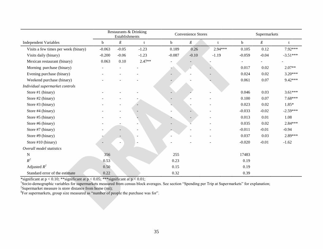
35

Restaurants & Drinking

Establishments Convenience Stores

Supermarkets

Independent Variables b ß t b ß t b ß t

Visits a few times per week (binary) -0.063 -0.05 -1.23

0.189 0.26 2.94 *** 0.105 0.12 7.92 ***

Visits daily (binary) -0.200 -0.06 -1.23

-0.087 -0.10 -1.19

-0.059 -0.04 -3.51 ***

Mexican restaurant (binary) 0.063 0.10 2.47 ** - - -

- - -

Morning purchase (binary) - - -

- - -

0.017 0.02 2.07 **

Evening purchase (binary) - - -

- - -

0.024 0.02 3.20 ***

Weekend purchase (binary) - - -

- - -

0.061 0.07 9.42 ***

Individual supermarket controls

Store #1 (binary) - - -

- - -

0.046 0.03 3.61 ***

Store #2 (binary) - - -

- - -

0.100 0.07 7.68 ***

Store #3 (binary) - - -

- - -

0.023 0.02 1.85 *

Store #4 (binary) - - -

- - -

-0.033 -0.02 -2.59 ***

Store #5 (binary) - - -

- - -

0.013 0.01 1.08

Store #6 (binary) - - -

- - -

0.035 0.02 2.84 ***

Store #7 (binary) - - -

- - -

-0.011 -0.01 -0.94

Store #9 (binary) - - -

- - -

0.037 0.03 2.89 ***

Store #10 (binary) - - -

- - -

-0.020 -0.01 -1.62

Overall model statistics

N 356

255

17483

R2 0.53

0.23

0.19

Adjusted R2 0.50

0.15

0.19

Standard error of the estimate 0.22 0.32 0.39

*significant at p < 0.10; **significant at p < 0.05; ***significant at p < 0.01; †Socio-demographic variables for supermarkets measured from census block averages. See section “Spending per Trip at Supermarkets” for explanation;

‡Supermarket measure is store distance from home (mi);

§For supermarkets, group size measured as “number of people the purchase was for”.

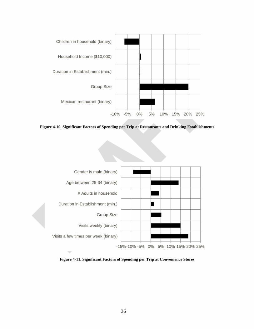
36

Figure 4-10. Significant Factors of Spending per Trip at Restaurants and Drinking Establishments

Figure 4-11. Significant Factors of Spending per Trip at Convenience Stores

-10% -5% 0% 5% 10% 15% 20% 25%

Mexican restaurant (binary)

Group Size

Duration in Establishment (min.)

Household Income ($10,000)

Children in household (binary)

-15%-10% -5% 0% 5% 10% 15% 20% 25%

Visits a few times per week (binary)

Visits weekly (binary)

Group Size

Duration in Establishment (min.)

# Adults in household

Age between 25-34 (binary)

Gender is male (binary)

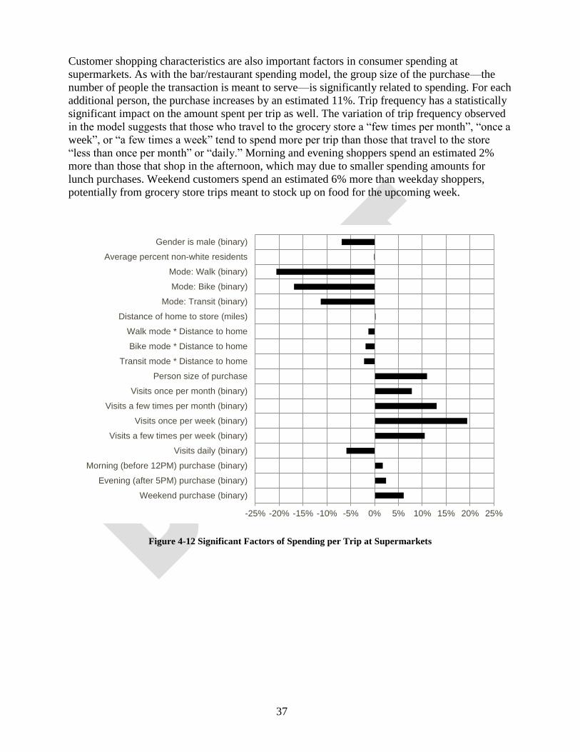
37

Customer shopping characteristics are also important factors in consumer spending at

supermarkets. As with the bar/restaurant spending model, the group size of the purchase—the

number of people the transaction is meant to serve—is significantly related to spending. For each

additional person, the purchase increases by an estimated 11%. Trip frequency has a statistically

significant impact on the amount spent per trip as well. The variation of trip frequency observed

in the model suggests that those who travel to the grocery store a “few times per month”, “once a

week”, or “a few times a week” tend to spend more per trip than those that travel to the store

“less than once per month” or “daily.” Morning and evening shoppers spend an estimated 2%

more than those that shop in the afternoon, which may due to smaller spending amounts for

lunch purchases. Weekend customers spend an estimated 6% more than weekday shoppers,

potentially from grocery store trips meant to stock up on food for the upcoming week.

Figure 4-12 Significant Factors of Spending per Trip at Supermarkets

-25% -20% -15% -10% -5% 0% 5% 10% 15% 20% 25%

Weekend purchase (binary)

Evening (after 5PM) purchase (binary)

Morning (before 12PM) purchase (binary)

Visits daily (binary)

Visits a few times per week (binary)

Visits once per week (binary)

Visits a few times per month (binary)

Visits once per month (binary)

Person size of purchase

Transit mode * Distance to home

Bike mode * Distance to home

Walk mode * Distance to home

Distance of home to store (miles)

Mode: Transit (binary)

Mode: Bike (binary)

Mode: Walk (binary)

Average percent non-white residents

Gender is male (binary)

38

SUMMARY

This chapter describes the analysis of mode shares of customers at a variety of business types,

locations, and transportation contexts, the analysis of connections between establishment-level

mode splits and the built environment, and the analysis of the links between consumer spending

and frequency of visits with travel modes. We find important differences in the relative mode

shares across these different business types based upon their location in the region and the

attributes of the built environment that support or detract from the use of various modes. There

are also clear distinctions in the average amounts spent per trip and the frequency of travel by

customers’ mode of access. But when these differences are examined more closely in models of

spending that control for the various demographic and other characteristics of consumers, these

differences by mode disappear, except in the case of supermarkets. These results have important

implications for planning and the impacts on local business community. We will discuss these

findings and what this may mean for transportation planning and local economies in more depth

in the next section.

39

Conclusions Chapter 5

This study is a first attempt to answer a few of the questions that have arisen concerning the

multimodal transportation investments and the impacts of mode shifts on the business

community. This research aims to merge the long history of scholarly work that examines of the

impacts of the built environment on non-work travel with the relatively new interest in consumer

spending by mode of travel. This empirical study of travel choices and consumer spending across

89 businesses in the Portland metropolitan area shows there are important differences between

the amounts customers spend on average by their mode of travel. However, these differences

become less pronounced when we control for demographics of the customer and other attributes

of the trip. This chapter starts with a discussion of these findings and the implications for

businesses. Then, we discuss some of the limitations of this study and a few considerations for

future work.

DISCUSSION

This study of consumer spending and travel choices has some compelling findings that suggest

some key spending and frequency differences by mode of travel that will likely invigorate the

discussion of the economic impacts of these modes. There are some results that are perhaps less

surprising. For these non-work destinations, the automobile remains the dominant mode of

travel. Patrons are largely arriving by private vehicle to most of the destinations in this study,

particularly to grocery stores where larger quantities of goods tend to be purchased. However,

important differences exist in the mode shares based upon the type and location of the

establishment and the levels of accommodation for a various modes.

The built environment matters. We see clear differences in the use of walking, bicycling, and

transit modes based upon the establishment location within the greater urban context, i.e. central

business district, town centers, commercial corridors, etc. The amount of activity, reflected by

residential and employment density, the proximity to rail transit, the presence of bike

infrastructure, and the amount of automobile and bicycle parking are all important in explaining

the use of non-automobile modes. The site design, while not explicitly examined here, seems to

play a role as well. The results suggest that businesses located in shopping centers see more

automobile travel than those located elsewhere. These shopping centers were dominated by large

parking lots that separated establishments from transit stops and had little consideration for bike

or pedestrian circulation within the site.

In terms of bicycling specifically, the built environment features that the literature has shown to

be associated with lower rates of automobile use and greater bicycling mode share were also

significant in this study. The directness of routes and connectivity was an important predictor of

customers choosing this mode. Intersection density is used as the measure of street design, but it

is also highly correlated with and a proxy for density, mixed use, block sizes, orthogonal street

layout and an older era of development. Convenient and abundant bicycle parking, including that

provided by on-street bike corrals, is associated with higher bicycle use by customers. However,

the direction of influence is not always clear. These corrals have historically been installed at the

request of businesses with a large share of bicycling patrons, although the practice of allocating

this kind of bicycle parking is changing. Thus, corrals may merely be an indicator of businesses

that already have a high bicycle mode share, rather than a causal factor in increased bicycle use.

Finally, bicycle facilities located on streets with high automobile traffic seem to deter the levels

40

of patronage of nearby businesses by bicyclists. While the presence of a bike lane on these busy

streets may provide better accommodation, it may be that cyclists use these as through routes,

rather than for local access. It also may mean that businesses located along these high vehicular

corridors are more likely to cater to the automobile than bicycling.

Advocates have long suggested that automobile trips of shorter lengths may be more amenable to

substitution by other modes. Portland has tried to incorporate this into the Portland Plan (2012)

by introducing the concept of the “20-minute neighborhood”, where residents can walk or bike to

meet their non-work needs. In addition, Joe Cortright (2007) has suggested that the urban growth

boundary has led to shorter trips, even by those made by automobile, and the resulting reductions

in transportation expenditures impart a “green dividend” to residents. While the results of this

study cannot confirm this green dividend theory, they do suggest that it is worth exploring

further. For example, in this study, the businesses in this study have at least 30% of their

customers traveling less than one mile, on average, to access the establishment. Similarly, the

majority of trips are less than 3 miles, although not all of these trips originate from home. These

results suggest the potential for substitution by walking, bicycling, and transit if they are not

already made by those modes.

The consumer spending results also contribute to this “green dividend” idea, although we cannot

confirm this theory without more research. On average, we see important differences in

consumer spending across the businesses in this study per trip and by mode of access. But

customers who walk, bicycle, and take transit have a greater frequency of trips on average than

those who drive for all of business types. This was a surprising result for bars and restaurants

where the hauling of purchases is not a consideration and lends some support for Cortright’s

supposition that the use of non-automobile modes may lead to greater capacity for individuals to

spend money on other things besides transportation.

These differences in trip frequency are key to the customers’ monthly spending patterns. Once

trip frequency is accounted for, the average monthly expenditures by customer modes of travel

reveal that bicyclists, transit users, and pedestrians are competitive consumers and for all

businesses except supermarkets, spend more, on average than those who drive. The greater

numbers of trips to these establishments also mean that these are regular customers, returning to

the establishment more often. Managers and business owners perhaps have greater opportunities

to get to know this segment of their market and cater to this constituency.

The analysis here examines average spending behaviors more closely and attempts to untangle

whether these differences in spending are due to customers’ mode of travel or other personal

characteristics that might be associated with their transportation choices. Indeed, the model

results indicate that the mode choice itself has little bearing on expenditures, except in the case

of supermarkets. Once the characteristics of customers are controlled for the mode of

transportation is not a significant contributor to the amount spent per trip at restaurants, bars, and

convenience stores. This is somewhat reassuring news for those concerned about the impacts of

shifting patronage away from automobile users. This suggests that it is not the mode itself that

matters but the characteristics of the people making these choices.

On the other hand, this raises the question of how these results might hold over the long term if

we aim to shift travel choices away from the automobile and towards more sustainable modes of

transportation. For example, if the aim of new infrastructure investments in bicycling is to attract

from those “interested but concerned” about bicycling, the impact on local businesses may

depend more upon the characteristics of this new group of bicyclists, which may differ

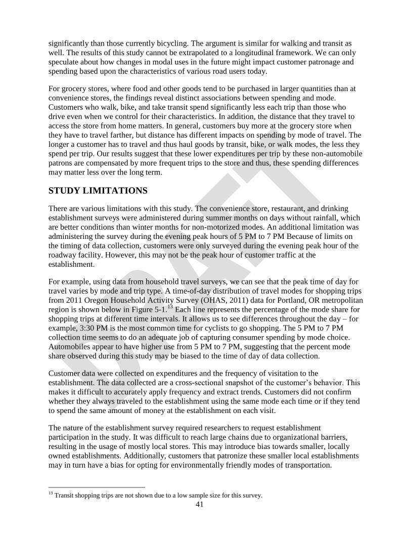
41

significantly than those currently bicycling. The argument is similar for walking and transit as

well. The results of this study cannot be extrapolated to a longitudinal framework. We can only

speculate about how changes in modal uses in the future might impact customer patronage and

spending based upon the characteristics of various road users today.

For grocery stores, where food and other goods tend to be purchased in larger quantities than at

convenience stores, the findings reveal distinct associations between spending and mode.

Customers who walk, bike, and take transit spend significantly less each trip than those who

drive even when we control for their characteristics. In addition, the distance that they travel to

access the store from home matters. In general, customers buy more at the grocery store when

they have to travel farther, but distance has different impacts on spending by mode of travel. The

longer a customer has to travel and thus haul goods by transit, bike, or walk modes, the less they

spend per trip. Our results suggest that these lower expenditures per trip by these non-automobile

patrons are compensated by more frequent trips to the store and thus, these spending differences

may matter less over the long term.

STUDY LIMITATIONS

There are various limitations with this study. The convenience store, restaurant, and drinking

establishment surveys were administered during summer months on days without rainfall, which

are better conditions than winter months for non-motorized modes. An additional limitation was

administering the survey during the evening peak hours of 5 PM to 7 PM Because of limits on

the timing of data collection, customers were only surveyed during the evening peak hour of the

roadway facility. However, this may not be the peak hour of customer traffic at the

establishment.

For example, using data from household travel surveys, we can see that the peak time of day for

travel varies by mode and trip type. A time-of-day distribution of travel modes for shopping trips

from 2011 Oregon Household Activity Survey (OHAS, 2011) data for Portland, OR metropolitan

region is shown below in Figure 5-1.13

Each line represents the percentage of the mode share for

shopping trips at different time intervals. It allows us to see differences throughout the day – for

example, 3:30 PM is the most common time for cyclists to go shopping. The 5 PM to 7 PM

collection time seems to do an adequate job of capturing consumer spending by mode choice.

Automobiles appear to have higher use from 5 PM to 7 PM, suggesting that the percent mode

share observed during this study may be biased to the time of day of data collection.

Customer data were collected on expenditures and the frequency of visitation to the

establishment. The data collected are a cross-sectional snapshot of the customer’s behavior. This

makes it difficult to accurately apply frequency and extract trends. Customers did not confirm

whether they always traveled to the establishment using the same mode each time or if they tend

to spend the same amount of money at the establishment on each visit.

The nature of the establishment survey required researchers to request establishment

participation in the study. It was difficult to reach large chains due to organizational barriers,

resulting in the usage of mostly local stores. This may introduce bias towards smaller, locally

owned establishments. Additionally, customers that patronize these smaller local establishments

may in turn have a bias for opting for environmentally friendly modes of transportation.

13

Transit shopping trips are not shown due to a low sample size for this survey.

42

Figure 5-1. Time-of-day Distribution of Travel Modes

Due to a large amount of customer personal information being omitted from the grocery store

survey (income, age, race, etc.), information available from the 2009 American Community

Survey and the 2010 U.S. Census for the Census block group where the customer lived were

used to proxy for or impute the household level socioeconomic data. More detailed information

about customers at grocery stores and their demographics would improve this study.

There may be limitations in generalizing these results to other U.S. cities. This study was

conducted in the metropolitan region of Portland, Oregon, which boasts higher than average non-

automobile mode usage. More study in other regions is needed to fully understand the link

between mode choice and consumer spending.

FUTURE CONSIDERATIONS

This study, while perhaps the first of its kind in the US, is certainly not the last. Although the

study provides important evidence that suggests that customers that access establishments by

non-automobile modes are competitive consumers and are important patrons for these

businesses, more research is needed to understand the implications of mode shifts away from the

automobile. In a climate of constrained financial resources for transportation, cities are asking

more detailed and difficult questions about what returns they are getting from transportation

Shopping trips

OHAS 2011

N

Bike: 34

Vehicle: 1,432

Walk: 174

Survey time period,

5 PM to 7 PM

43

investments that expand beyond demand and facility usage to consider broader economic

benefits.

As cities making changes to better accommodate bicycling, walking, and transit and encourage a

range of transportation choices, it is unclear where shifts away from the automobile may lead.

The results from this study are encouraging for local businesses but this research is limited in its

reach. For example, a business owner that questions the impact of adding bike corrals at the

expense automobile parking will not find definitive answers about the optimal combination that

creates the greatest return. This will require a more in-depth study of longitudinal customer

behaviors as well as the relative costs to businesses to provide accommodation for various

modes, including capital and operating costs.

Again, a longitudinal framework is needed capture changes in behavior, including mode shifts,

frequency of trips and changes in spending. So should an establishment become more

accommodating for non-motorized modes, it is not clear whether the business will see changes

among its current customer base and their trip making behavior (modes, frequencies and times of

day/days of week) or if their customer base grow or shrink, attracting perhaps patrons who have

different modal preferences and shopping behaviors.

Finally, we must acknowledge that travel behavior is complex and multi-modal. Single mode use

is rare. We use multiple modes for multiple purposes and there is much variation in our behavior.

The bicyclists included in our study may travel by automobile, walking, or transit to access many

of their activities and on different days, times or seasons, and may vary their mode choices to

access even the same destination. Therefore, our research must take serious consideration of our

multimodal nature and find ways to accommodate this in our planning practice. US cities are

working to provide more transportation options – including more flexible vehicle and bicycle

sharing – that can change the way we think about our daily travel and routines. We are no longer

bound to travel by the mode use to leave our homes and this is like going to impact not only our

travel patterns but our consumer behavior as well.

44

References Chapter 6

Bawa, K, and Ghosh. “A Model of Household Grocery Shopping Behavior,” Marketing Letters,

Vol. 10, 1999. pp. 149-160.

Bent, E. and Singa, K. “Modal Choices and Spending Patterns of Travelers to Downtown San

Francisco, California: Impacts on of Congestion Pricing on Retail Trade,” Transportation

Research Record: Journal of the Transportation Research Board, No. 2115, Transportation

Research Board of the National Academies, Washington D.C., Transportation Record, 2009, pp.

66-74.

US Bureau of Labor Statistics. “Consumer Expenditures – 2011,” Economic news release,

accessed online, 2012.

Cao, X., P.L. Mokhtarian, and S.L. Handy. “Examining the Impacts of Residential Self-

Selection on Travel Behaviour: A Focus on Empirical Findings,” Transport Reviews, Volume

29, pp. 359-395, 2009.

CBC News. “Vancouver Bike Lanes to Stay, City Council Decides,” Accessed online, 2012.

Cervero, R. (2006). “Effects of Light and Commuter Rail Transit on Land Prices: Experiences in

San Diego County.” University of California Transportation Center, Faculty Research Paper,

#769.

Cervero, R. and K. Kockelman. “Travel Demand and the 3Ds: Density, Diversity, and Design,”

Transportation Research Part D: Transport and Environment, Volume 2, Issue 3, pp. 199-219,

September 1997.

Cortright, J. “Portland’s Green Dividend,” White Paper, CEOs for Cities, 2007.

Dill, Jennifer and Carr, Theresa. “Bicycle Commuting and Facilities in Major U.S. Cities: If You

Build Them, Commuters Will Use Them,” Transportation Research Record: Journal of the

Transportation Research Board, vol. 1828, 2003. pp. 116-123.

Drennen, E. “Economic Effects of Traffic Calming on Urban Small Businesses,” Department of

Public Administration, San Francisco State University. 2003.

Ewing, R. and R. Cervero. “Travel and the Built Environment: A Meta-Analysis,” Journal of the

American Planning Association, Volume 76, Number 3, pp. 1-30, Summer 2010.

Fietsberaad News Report. “Cyclists spend as much in supermarket as motorists,” May 23, 2011.

Fietsberaad.

Forkes, Jennifer, and Lea, Nancy. “Bike Lanes, On-Street Parking, and Business, Year 2 Report:

A Study of Bloor Street in Toronto’s Bloor West Village,” Prepared for the Clean Air

Partnership, 2011.

Grant, J. and K. Perrot. “Where is the Café? The Challenge of Making Retail Uses Viable in

Mixed-use Suburban Developments,” Urban Studies, Volume 48, Issue 1, pp. 177-195, 2011.

45

Handy, S. “A Cycle of Dependence: Automobiles, Accessibility, and the Evolution of the

Transportation and Retail Hierarchies,” Berkeley Planning Journal, Volume 8, pp. 21-43, 1993.

Handy, S. and K. J. Clifton. “Local Shopping as a Strategy for Reducing Automobile Travel,”

Transportation, Volume 28, pp. 317–346, 2001.

Jiao, J., A.V. Moudon and A. Drewnowski. “Grocery Shopping: How individuals and built

environments influence travel mode choice,” Transportation Research Record: Journal of the

Transportation Research Board, CD-ROM. No. 11-2322, Transportation Research Board of the

National Academies, Washington D.C., Transportation Record, 2011.

Jones, Peter, and Peter R. Stopher. “Transport survey quality and innovation,” Emerald Group

Publishing, 2003.

Kim, B and Park, K. “Studying Patterns of Consumer's Grocery Shopping Trip,” Journal of

Retailing, Vol. 73, 1997. pp. 501-517.

Lee, A. “What Is The Economic Contribution Of Cyclists Compared To Car Drivers In Inner

Suburban Melbourne’s Shopping Strips?,” University of Melbourne. Melbourne, Australia, 2008.

Master's Thesis.

McConville, Megan; Rodríguez, Daniel A. , Clifton, Kelly J; Cho, Gihyoug, and Fleischhacker,

Sheila. “Disaggregate Land Uses and Walking,” American Journal of Preventive Medicine,

Volume 40, Issue 1, January 2011. pp 25-32.

Meisel, D. Bike Corrals: Local Business Impacts, Benefits, and Attitudes. Portland State

University School of Urban Studies and Planning. 2010.

New York City DOT. “Measuring the Streets: New Metrics for 21st Century Streets,” 2012.

Oregon Travel & Activity Survey (OHAS or OTAS), Oregon Department of Transportation,

2009-2011.

The Portland Plan. 2012. City of Portland, Oregon. Available online at http://pdxplan.com

Pucher, John, and Buehler, Ralph. “Why Canadians cycle more than Americans: A comparative

analysis of bicycling trends and policies,” Institute of Transport and Logistics Studies, 2005.

Pucher, John; Komanoff, Charles, and Schimek, Paul. “Bicycling renaissance in North America?

Recent trends and alternative policies to promote bicycling,” Transportation Research Part A,

Vol. 33, 1999. pp. 625-654.

Rodriguez, D. A., and J. Joo. “The Relationship Between Non-Motorized Mode Choice And The

Local Physical Environment,” Transportation Research Part D, Volume 9, pp. 151-173, 2004.

Stantec Consulting Ltd, Site Economics, and Mustel Group Market Research. “Vancouver

Separated Bike Lane Business Impact Study,” Prepared for the Vancouver Economic

Development Commission, City of Vancouver, Downtown Vancouver Association, Downtown

Vancouver Business Improvement Association, The Vancouver Board of Trade, 2011.

46

Steiner, Ruth. “Trip Generation and Parking Requirements in Traditional Shopping Districts,”

Transportation Research Record: Journal of the Transportation Research Board, vol. 1617,

1998. pp 28-37.

Sustrans, UK. “Shoppers and How they Travel,” Livable Neighborhoods information sheet, 2006

Sztabinski, F. Bike Lanes, On-street Parking, and Business: A Study of Bloor Street in Toronto’s

Annex Neighborhood. The Clean Air Partnership. 2009.

Targa, Felipe and Clifton, Kelly J. (corresponding author). “The built environment and trip

generation for non-motorized travel,” Journal of Transportation and Statistics, vol. 8(3), 2005.

pp. 55-70.

Transportation Alternatives. “East Village Shoppers Study, a Snapshot of Travel and Spending

Patterns of Residents and Visitors in the East Village,” 2012.

Trendy Travel. “Trendy Cycling,” Report produced by Trendy Travel in conjunction with

Intelligent Energy Europe, 2010.

Zhang, M. “The Role of Land Use in Travel Mode Choice: Evidence From Boston and Hong

Kong,” Journal of American Planning Association, Volume 70, Issue 3, pp. 344-361, 2004.

47

Appendices

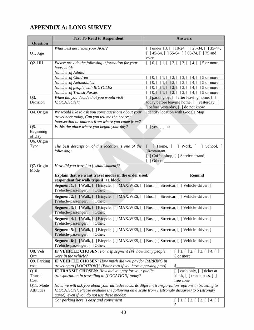
48

APPENDIX A: LONG SURVEY

Question

Text To Read to Respondent Answers

Q1. Age

What best describes your AGE? [ ] under 18, [ ] 18-24, [ ] 25-34, [ ] 35-44,

[ ] 45-54, [ ] 55-64, [ ] 65-74, [ ] 75 and

over

Q2. HH Please provide the following information for your

household:

Number of Adults

[ ] 0, [ ] 1, [ ] 2, [ ] 3, [ ] 4, [ ] 5 or more

Number of Children [ ] 0, [ ] 1, [ ] 2, [ ] 3, [ ] 4, [ ] 5 or more

Number of Automobiles [ ] 0, [ ] 1, [ ] 2, [ ] 3, [ ] 4, [ ] 5 or more

Number of people with BICYCLES [ ] 0, [ ] 1, [ ] 2, [ ] 3, [ ] 4, [ ] 5 or more

Number of Transit Passes [ ] 0, [ ] 1, [ ] 2, [ ] 3, [ ] 4, [ ] 5 or more

Q3.

Decision

When did you decide that you would visit

[LOCATION]?

[ ] passing by, [ ] after leaving home, [ ]

today before leaving home, [ ] yesterday, [

] before yesterday, [ ] do not know

Q4. Origin We would like to ask you some questions about your

travel here today, Can you tell me the nearest

intersection or address from where you came from?

Identify location with Google Map

Q5.

Beginning

of Day

Is this the place where you began your day? [ ] yes, [ ] no

Q6. Origin

Type The best description of this location is one of the

following:

[ ] Home, [ ] Work, [ ] School, [

]Restaurant,

[ ] Coffee shop, [ ] Service errand,

[ ] Other: __________________

Q7. Origin

Mode

How did you travel to [establishment]?

Explain that we want travel modes in the order used. Remind

respondent for walk trips if >1 block.

Segment 1: [ ] Walk, [ ] Bicycle, [ ] MAX/WES, [ ] Bus, [ ] Streetcar, [ ] Vehicle-driver, [

]Vehicle-passenger, [ ] Other:______________

Segment 2: [ ] Walk, [ ] Bicycle, [ ] MAX/WES, [ ] Bus, [ ] Streetcar, [ ] Vehicle-driver, [

]Vehicle-passenger, [ ] Other:______________

Segment 3: [ ] Walk, [ ] Bicycle, [ ] MAX/WES, [ ] Bus, [ ] Streetcar, [ ] Vehicle-driver, [

]Vehicle-passenger, [ ] Other:______________

Segment 4: [ ] Walk, [ ] Bicycle, [ ] MAX/WES, [ ] Bus, [ ] Streetcar, [ ] Vehicle-driver, [

]Vehicle-passenger, [ ] Other:______________

Segment 5: [ ] Walk, [ ] Bicycle, [ ] MAX/WES, [ ] Bus, [ ] Streetcar, [ ] Vehicle-driver, [

]Vehicle-passenger, [ ] Other:______________

Segment 6: [ ] Walk, [ ] Bicycle, [ ] MAX/WES, [ ] Bus, [ ] Streetcar, [ ] Vehicle-driver, [

]Vehicle-passenger, [ ] Other:______________

Q8. Veh

Occ

IF VEHICLE CHOSEN: For trip segment [#], how many people

were in the vehicle?

[ ] 1, [ ] 2, [ ] 3, [ ] 4, [ ]

5 or more

Q9. Parking

cost

IF VEHICLE CHOSEN: How much did you pay for PARKING in

traveling to [LOCATION]? (Enter zero if you have a parking pass)

$_________

Q10.

Transit

Cost

IF TRANSIT CHOSEN: How did you pay for your public

transportation in travelling to [LOCATION] today?

[ ] cash only, [ ] ticket at

kiosk, [ ] transit pass, [ ]

free zone

Q11. Mode

Attitudes

Now, we will ask you about your attitudes towards different transportation options in traveling to

[LOCATION]. Please evaluate the following on a scale from 1 (strongly disagree) to 5 (strongly

agree), even if you do not use these modes:

Car parking here is easy and convenient [ ] 1, [ ] 2, [ ] 3, [ ] 4, [ ]

5

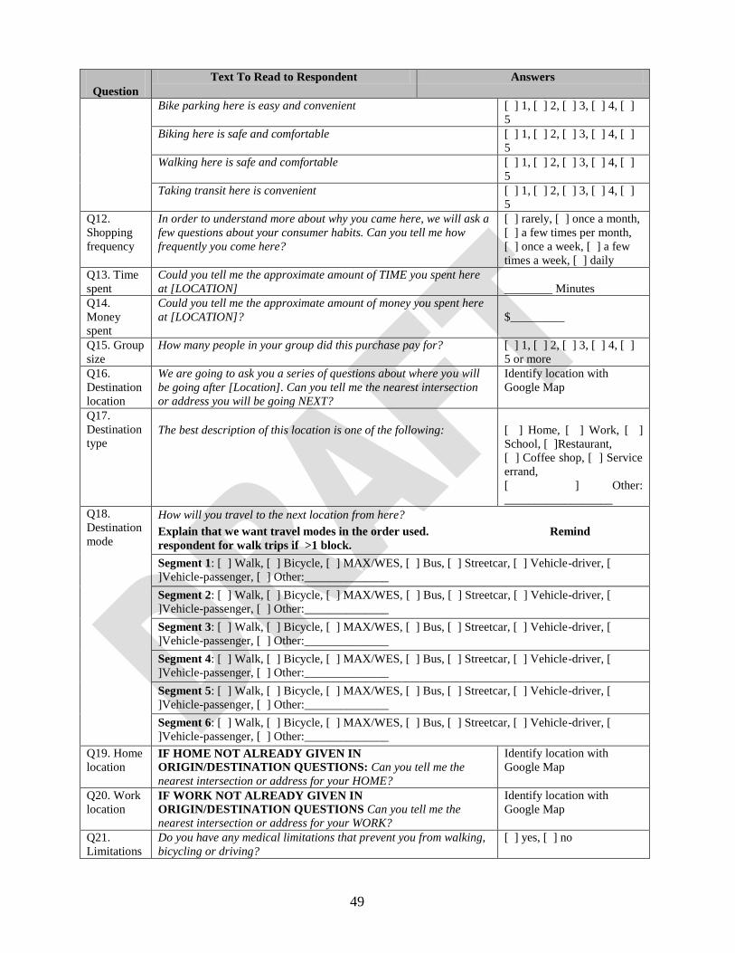
49

Question

Text To Read to Respondent Answers

Bike parking here is easy and convenient [ ] 1, [ ] 2, [ ] 3, [ ] 4, [ ]

5

Biking here is safe and comfortable [ ] 1, [ ] 2, [ ] 3, [ ] 4, [ ]

5

Walking here is safe and comfortable [ ] 1, [ ] 2, [ ] 3, [ ] 4, [ ]

5

Taking transit here is convenient [ ] 1, [ ] 2, [ ] 3, [ ] 4, [ ]

5

Q12.

Shopping

frequency

In order to understand more about why you came here, we will ask a

few questions about your consumer habits. Can you tell me how

frequently you come here?

[ ] rarely, [ ] once a month,

[ ] a few times per month,

[ ] once a week, [ ] a few

times a week, [ ] daily

Q13. Time

spent

Could you tell me the approximate amount of TIME you spent here

at [LOCATION]

________ Minutes

Q14.

Money

spent

Could you tell me the approximate amount of money you spent here

at [LOCATION]?

$_________

Q15. Group

size

How many people in your group did this purchase pay for? [ ] 1, [ ] 2, [ ] 3, [ ] 4, [ ]

5 or more

Q16.

Destination

location

We are going to ask you a series of questions about where you will

be going after [Location]. Can you tell me the nearest intersection

or address you will be going NEXT?

Identify location with

Google Map

Q17.

Destination

type The best description of this location is one of the following:

[ ] Home, [ ] Work, [ ]

School, [ ]Restaurant,

[ ] Coffee shop, [ ] Service

errand,

[ ] Other:

__________________

Q18.

Destination

mode

How will you travel to the next location from here?

Explain that we want travel modes in the order used. Remind

respondent for walk trips if >1 block.

Segment 1: [ ] Walk, [ ] Bicycle, [ ] MAX/WES, [ ] Bus, [ ] Streetcar, [ ] Vehicle-driver, [

]Vehicle-passenger, [ ] Other:______________

Segment 2: [ ] Walk, [ ] Bicycle, [ ] MAX/WES, [ ] Bus, [ ] Streetcar, [ ] Vehicle-driver, [

]Vehicle-passenger, [ ] Other:______________

Segment 3: [ ] Walk, [ ] Bicycle, [ ] MAX/WES, [ ] Bus, [ ] Streetcar, [ ] Vehicle-driver, [

]Vehicle-passenger, [ ] Other:______________

Segment 4: [ ] Walk, [ ] Bicycle, [ ] MAX/WES, [ ] Bus, [ ] Streetcar, [ ] Vehicle-driver, [

]Vehicle-passenger, [ ] Other:______________

Segment 5: [ ] Walk, [ ] Bicycle, [ ] MAX/WES, [ ] Bus, [ ] Streetcar, [ ] Vehicle-driver, [

]Vehicle-passenger, [ ] Other:______________

Segment 6: [ ] Walk, [ ] Bicycle, [ ] MAX/WES, [ ] Bus, [ ] Streetcar, [ ] Vehicle-driver, [

]Vehicle-passenger, [ ] Other:______________

Q19. Home

location IF HOME NOT ALREADY GIVEN IN

ORIGIN/DESTINATION QUESTIONS: Can you tell me the

nearest intersection or address for your HOME?

Identify location with

Google Map

Q20. Work

location IF WORK NOT ALREADY GIVEN IN

ORIGIN/DESTINATION QUESTIONS Can you tell me the

nearest intersection or address for your WORK?

Identify location with

Google Map

Q21.

Limitations

Do you have any medical limitations that prevent you from walking,

bicycling or driving?

[ ] yes, [ ] no

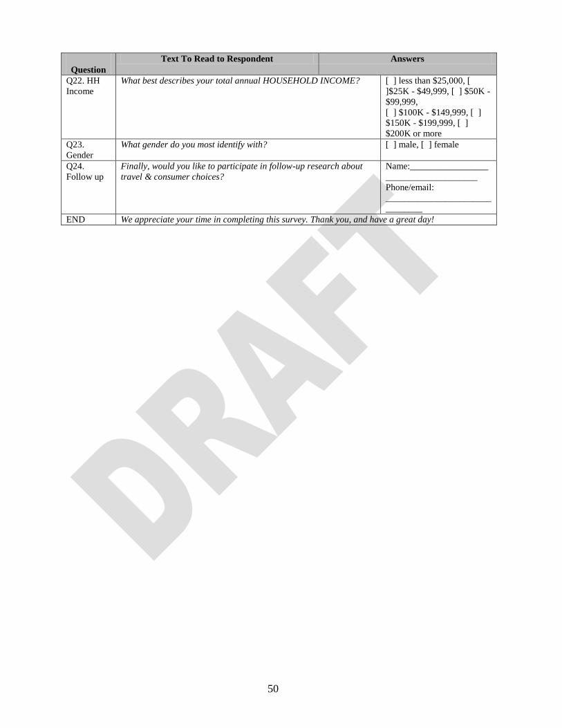
50

Question

Text To Read to Respondent Answers

Q22. HH

Income

What best describes your total annual HOUSEHOLD INCOME? [ ] less than $25,000, [

]$25K - $49,999, [ ] $50K -

$99,999,

[ ] $100K - $149,999, [ ]

$150K - $199,999, [ ]

$200K or more

Q23.

Gender

What gender do you most identify with? [ ] male, [ ] female

Q24.

Follow up

Finally, would you like to participate in follow-up research about

travel & consumer choices?

Name:_________________

____________________

Phone/email:

_______________________

________

END We appreciate your time in completing this survey. Thank you, and have a great day!

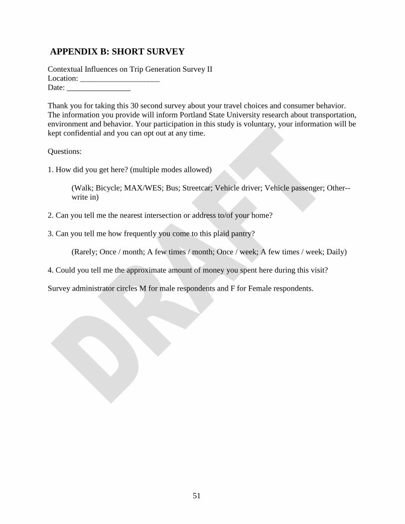
51

APPENDIX B: SHORT SURVEY

Contextual Influences on Trip Generation Survey II

Location: ____________________

Date: ________________

Thank you for taking this 30 second survey about your travel choices and consumer behavior.

The information you provide will inform Portland State University research about transportation,

environment and behavior. Your participation in this study is voluntary, your information will be

kept confidential and you can opt out at any time.

Questions:

1. How did you get here? (multiple modes allowed)

(Walk; Bicycle; MAX/WES; Bus; Streetcar; Vehicle driver; Vehicle passenger; Other--

write in)

2. Can you tell me the nearest intersection or address to/of your home?

3. Can you tell me how frequently you come to this plaid pantry?

(Rarely; Once / month; A few times / month; Once / week; A few times / week; Daily)

4. Could you tell me the approximate amount of money you spent here during this visit?

Survey administrator circles M for male respondents and F for Female respondents.

52

APPENDIX C: GROCERY STORE SURVEY

Question

Text for Respondent Answers

Q1

Where do you live? Please click on home location

on map. Identify home location with Google Map

Q2 How did you get here today? [ ] Walk [ ] Bike [ ] Car [ ] Bus [ ] MAX

[ ] Other

Q3 Did you come from home? [ ] Yes [ ] No

Q4 Please tell us exactly how much you spent at the

grocery store TODAY? Enter exact amount spent to the decimal

Q5 How often do you shop here?

[ ] Less than once a month [ ] Once a month

[ ] A few times a month [ ] Once a week [

] A few times a week [ ] Daily

Q6 Please tell us how many people you are shopping

for at the grocery store TODAY?

[ ] 1 person [ ] 2 people [ ] 3 people [ ] 4

people [ ] 5 or more people

Q7 What gender do you most identify with? [ ] Male [ ] Female [ ] Other

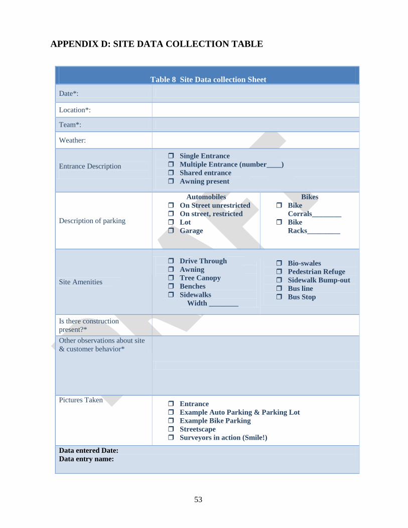
53

APPENDIX D: SITE DATA COLLECTION TABLE

Table 8 Site Data collection Sheet

Date*:

Location*:

Team*:

Weather:

Entrance Description

Single Entrance

Multiple Entrance (number____)

Shared entrance

Awning present

Description of parking

Automobiles

On Street unrestricted

On street, restricted

Lot

Garage

Bikes

Bike

Corrals________

Bike

Racks_________

Site Amenities

Drive Through

Awning

Tree Canopy

Benches

Sidewalks

Width ________

Bio-swales

Pedestrian Refuge

Sidewalk Bump-out

Bus line

Bus Stop

Is there construction

present?*

Other observations about site

& customer behavior*

Pictures Taken Entrance

Example Auto Parking & Parking Lot

Example Bike Parking

Streetscape

Surveyors in action (Smile!)

Data entered Date:

Data entry name: