Embed Size (px)
Citation preview
University of Cambridge
MPhil Thesis
Constructive Representation of
Nominal Sets in Agda
Author:
Pritam Choudhury
Robinson College
Supervisor:
Prof. Andrew M. Pitts
The Computer Laboratory
A dissertation submitted to the University of Cambridge
in partial fulfilment of the requirements for the degree of
Master of Philosophy in Advanced Computer Science
June 12, 2015

Declaration of Authorship
I, Pritam Choudhury of Robinson College, being a candidate for the M.Phil in Advanced
Computer Science, hereby declare that this report and the work described in it are my
own work, unaided except as may be specified below, and that the report does not
contain material that has already been used to any substantial extent for a comparable
purpose.
Total word count: 13758 (excluding all mathematical symbols)
Signed:
Date:
All trademarks used in this dissertation are hereby acknowledged.
ii

Abstract
The theory of nominal sets provide a mathematical analysis of names that is based
upon symmetry. It formalizes the informal reasoning we employ while working with
languages involving name binding operators. The central ideas of the theory are sup-
port, freshness and name abstraction, which respectively encapsulate the ideas of name
dependence, name independence and alpha equivalence. This theory has been devel-
oped within the framework of classical logic. Certain notions of this classical theory,
like the smallest finite support for an element of a nominal set, are non-constructive. In
this dissertation, we show that with appropriate modifications, a considerable portion
of the theory of nominal sets can also be developed constructively. We show this by
building from scratch, the theory of nominal sets, upto and including name abstraction
sets, in the dependent type-theoretic environment of the programming language Agda.
In our development, we replace the notion of unique smallest finite support with that of
non-unique some finite support. In addition, all throughout our development, we work
with setoids. This helps us in recovering extensionality of functions and in working with
alpha-equivalence classes of terms. Though extensionality of functions could have been
easily postulated in Agda, we refrained from using any postulate whatsoever at any level,
since we cannot ensure constructivity of the whole development in case it rests even on
just a single postulate. Our work can be extended and developed further to produce a
nominal version of Agda which would make working with binding constructs in Agda
much more easier.
iv

“A journey of a thousand miles must begin with a single step.”
Lao Tzu
Events, as they turned out
After completing my Bachelor’s degree in electrical engineering from Indian Institute
of Technology, Roorkee, India, when I came to Cambridge, I was supposed to study
natural language processing. But after attending classes for a week, I realized, natural
language processing was not my cup of tea. The one thing that I could not digest all
my life is ambiguity and handling ambiguity is one of the very important concerns of
natural language processing. So, I decided to switch over to the theoretical modules, in
retrospect, with incommensurate trust on my mathematical abilities. It was not long
before I found out that I literally knew nothing. The veracity of this statement can be
judged from the fact that at that time, I did not know what a lambda term is. But I
did not lose hope. Because though I could hardly follow the lectures technically, I got
the intuitions. The Category theory course, by Prof. Andrew M. Pitts, in particular,
opened unexplored territories in my mind. I liked all the ‘general abstract non-sense’.
So then, when I approached Prof. Pitts to suggest some mathematical project for my
MPhil ACS, he proposed that I work on ‘Constructive representation of nominal sets in
Agda’. At that time, I neither knew what ‘constructive’ is, nor did I know what nominal
sets are. Not to say anything about my knowledge of Agda, since I did not know any
programming language other than C++ and MATLAB. But I was determined to work
on the project. I argued with myself, this is the time to take risks, if not now, then never.
When I wrote the project proposal with the help of Prof. Pitts in late November last
year, I was hardly aware of the intensity of the challenges that lay ahead of me. The first
blow came when I started reading some Agda code developed by others. I was totally
confused. What is a type? What is the difference between a data type and a function
type? Why do propositions on a type map the elements of that type to ‘Set’? Prof.
Pitts answered these questions, but at that time, a new term was leading me to a whole
bunch of other even newer terms and I could see no end to this. The other problem was
that information about Agda is scattered across various tutorials, papers, code snippets,
etc. There is no single comprehensive guide to Agda covering the language in all its
details. So I was reading everything I could find, but all this reading did not lead to
an understanding of the language. With all these problems, two months passed. It was
mid February and I was almost at the point where I began, other than having known a
few technical terms here and there. It was clear that things were not working. At this
point, I changed all my plans. May be the top-down approach would not work. May
be I cannot possibly comprehend the profundity of dependent type theory, constructive
logic and Agda in a month or two and that any attempt towards that would just increase
confusion. But may be, I can still start working on Agda and Agda itself will teach me
how to deal with it. So then, I tried the bottom up approach. Slowly, but surely, it
worked. Starting from the point where writing a line or two in Agda required hours of
vi
thought amidst constant tussle with the type-checker to make it accept the definition I
was writing, I gradually moved to the point where I could just sit and start writing as if
I were doing maths on pen and paper, without really bothering about the type-checker,
out of confidence that if I can satisfy myself, the type-checker too will be satisfied. And
from that point onwards, things flowed, though not without occasional hiccups, but
those were petty things when compared with the challenges I had to overcome in the
initial days of the project.
This project then, was a medium of transformation for me, not just academically but
also from a broader perspective. I learnt how to face my fears, I learnt why not to fight
with them, but to swim along with them, for it’s fear that leads to all great truths,
when followed incessantly. I believe this lesson will help me face my future in a more
resourceful way.
And none of these would have been possible without Prof. Pitts. All throughout these
months, he has been an academic mentor and a moral supporter. Though I could not
gather everything that he had said in my initial supervisions, still I believe that those
meetings were very helpful, because they gave me the faith that may be things are not
that difficult, may be, like Andrew, I too can understand them some day. My thanks are
also due to Dr. Jeremy Yallop and Dr. Leo White, lecturers of the Advanced Functional
Programming course. Being completely new to functional programming, I could not
have worked with Agda, if this course were not there. And I cannot thank Jeremy and
Leo enough for how well they taught the course. My thanks also to other lecturers and
professors and other members of the Computer Laboratory, who have helped in different
ways at different times.

Contents
Declaration of Authorship ii
Abstract iv
Events, as they turned out vi
Contents ix
Symbols xi
1 Introduction 1
1.1 What’s in a name? . . . . . . . . . . . . . . . . . . . . . . . . . . . . . . . . . 1
1.2 Names and Symmetry . . . . . . . . . . . . . . . . . . . . . . . . . . . . . . . 2
1.3 Names in computer science . . . . . . . . . . . . . . . . . . . . . . . . . . . . 2
1.4 Literature review . . . . . . . . . . . . . . . . . . . . . . . . . . . . . . . . . . 3
1.5 Motivation . . . . . . . . . . . . . . . . . . . . . . . . . . . . . . . . . . . . . . 4
1.6 Related Work . . . . . . . . . . . . . . . . . . . . . . . . . . . . . . . . . . . . 6
1.7 Constructive logic . . . . . . . . . . . . . . . . . . . . . . . . . . . . . . . . . 6
1.8 Intuitionistic or Dependent type theory . . . . . . . . . . . . . . . . . . . . 7
1.9 Agda . . . . . . . . . . . . . . . . . . . . . . . . . . . . . . . . . . . . . . . . . 8
1.10 An example . . . . . . . . . . . . . . . . . . . . . . . . . . . . . . . . . . . . . 10
1.11 Structure of the thesis . . . . . . . . . . . . . . . . . . . . . . . . . . . . . . . 14
2 Permutations 16
2.1 Atoms . . . . . . . . . . . . . . . . . . . . . . . . . . . . . . . . . . . . . . . . 16
2.2 Finite permutations . . . . . . . . . . . . . . . . . . . . . . . . . . . . . . . . 17
2.3 Permutations are bijective functions . . . . . . . . . . . . . . . . . . . . . . 17
2.4 Equivalence relation on permutations . . . . . . . . . . . . . . . . . . . . . . 20
2.5 Group . . . . . . . . . . . . . . . . . . . . . . . . . . . . . . . . . . . . . . . . 20
2.6 Finite permutations form a group . . . . . . . . . . . . . . . . . . . . . . . . 21
2.7 Group Action . . . . . . . . . . . . . . . . . . . . . . . . . . . . . . . . . . . . 23
2.8 Examples of Group Action . . . . . . . . . . . . . . . . . . . . . . . . . . . . 23
2.9 Perm-Set . . . . . . . . . . . . . . . . . . . . . . . . . . . . . . . . . . . . . . . 26
2.10 Equivariant functions . . . . . . . . . . . . . . . . . . . . . . . . . . . . . . . 26
2.11 Example of an equivariant function . . . . . . . . . . . . . . . . . . . . . . . 27
2.12 Useful properties of permutations . . . . . . . . . . . . . . . . . . . . . . . . 27
ix
Contents x
2.12.1 Atoms unchanged under action . . . . . . . . . . . . . . . . . . . . . 27
2.12.2 A permutation and a name-swap . . . . . . . . . . . . . . . . . . . . 28
3 A category theoretic perspective 32
3.1 Nominal Set . . . . . . . . . . . . . . . . . . . . . . . . . . . . . . . . . . . . . 32
3.2 Examples of Nominal Sets . . . . . . . . . . . . . . . . . . . . . . . . . . . . 34
3.3 Functions between nominal sets . . . . . . . . . . . . . . . . . . . . . . . . . 36
3.4 Nom and Nomfs . . . . . . . . . . . . . . . . . . . . . . . . . . . . . . . . . 38
3.5 Products in Nom and Nomfs . . . . . . . . . . . . . . . . . . . . . . . . . . 40
3.6 Coproducts in Nom and Nomfs . . . . . . . . . . . . . . . . . . . . . . . . 40
3.7 Exponentials in Nom and Nomfs . . . . . . . . . . . . . . . . . . . . . . . 41
3.7.1 Exponential object . . . . . . . . . . . . . . . . . . . . . . . . . . . . 42
3.7.2 Application morphism . . . . . . . . . . . . . . . . . . . . . . . . . . 43
3.7.3 Currying in Nom . . . . . . . . . . . . . . . . . . . . . . . . . . . . 43
3.7.4 Currying in Nomfs . . . . . . . . . . . . . . . . . . . . . . . . . . . 45
3.8 Pullbacks in Nom . . . . . . . . . . . . . . . . . . . . . . . . . . . . . . . . . 45
3.9 Nom-sets and Perm-sets . . . . . . . . . . . . . . . . . . . . . . . . . . . . . . 47
3.10 Powerset . . . . . . . . . . . . . . . . . . . . . . . . . . . . . . . . . . . . . . . 49
4 Freshness 51
4.1 Definition . . . . . . . . . . . . . . . . . . . . . . . . . . . . . . . . . . . . . . 51
4.2 Some/any theorem . . . . . . . . . . . . . . . . . . . . . . . . . . . . . . . . . 52
4.3 Freshness in finitely supported functions . . . . . . . . . . . . . . . . . . . . 53
4.4 Separated product functor . . . . . . . . . . . . . . . . . . . . . . . . . . . . 54
5 Name Abstraction 57
5.1 Alpha-equivalence . . . . . . . . . . . . . . . . . . . . . . . . . . . . . . . . . 57
5.2 Name abstraction sets . . . . . . . . . . . . . . . . . . . . . . . . . . . . . . . 59
5.3 Name abstraction functor . . . . . . . . . . . . . . . . . . . . . . . . . . . . . 60
5.4 Properties of name abstraction functor . . . . . . . . . . . . . . . . . . . . . 61
5.5 Freshness condition for binders . . . . . . . . . . . . . . . . . . . . . . . . . 67
6 Conclusion 73
Bibliography 75
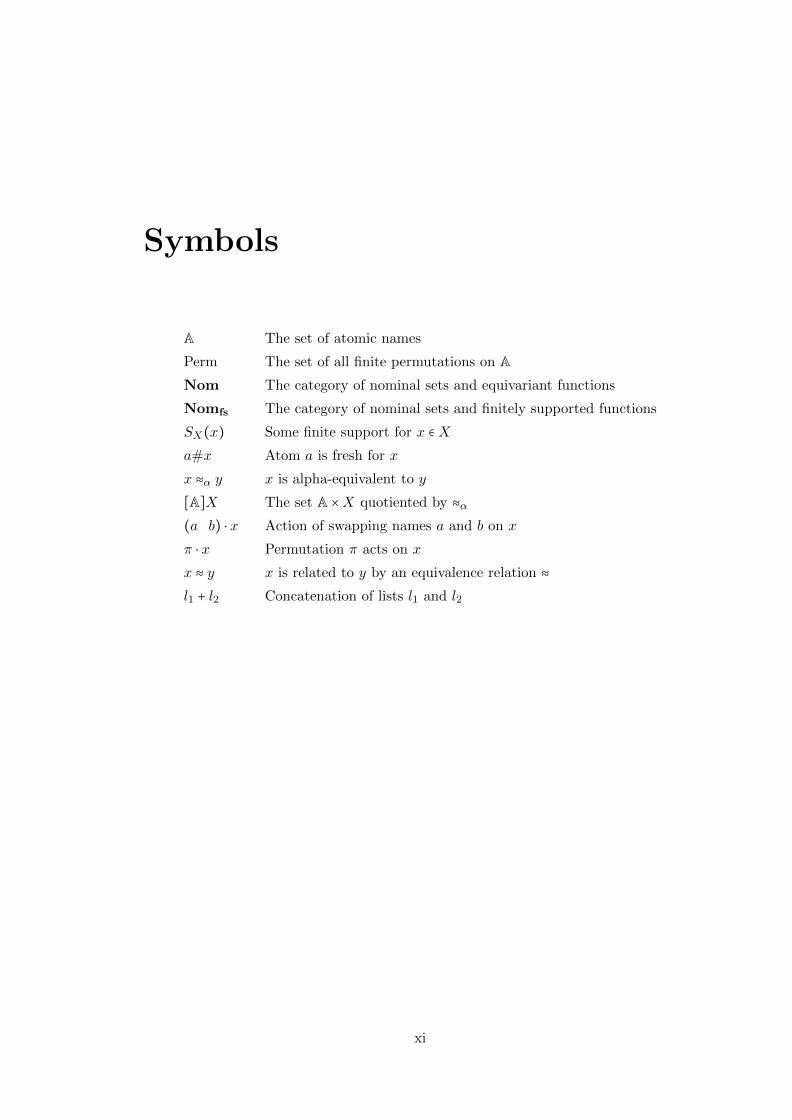
Symbols
A The set of atomic names
Perm The set of all finite permutations on ANom The category of nominal sets and equivariant functions
Nomfs The category of nominal sets and finitely supported functions
SX(x) Some finite support for x ∈X
a#x Atom a is fresh for x
x ≈α y x is alpha-equivalent to y
[A]X The set A ×X quotiented by ≈α
(a b) ⋅ x Action of swapping names a and b on x
π ⋅ x Permutation π acts on x
x ≈ y x is related to y by an equivalence relation ≈
l1 + l2 Concatenation of lists l1 and l2
xi

Chapter 1
Introduction
1.1 What’s in a name?
Imagine a Primordial Observer (PO), an entity which considers everything to be atomic
and thus unrelated to everything else. So, to PO, a certain table at a certain time
instant has no relation whatsoever to the same table at the very next moment. Indeed,
PO has no sense of meaning because any meaning attributed to any object would be
restricted to that very object at that very instant and thus would be of no use. But if
PO decides that certain instances of a given object can be unified under some property,
thus yielding a single object whose different instances are related to one another by that
property, then PO must coin a name for that object. Thus, any name represents a level
of abstraction relating different instances of the thing named. This is true even in the
case of algebraic variables used as names, since, for example, while using ‘x’ as a name
for the number of apples in a given problem, we implicitly apply the convention that
all occurrences of the variable ‘x’ in that problem refer to the number of apples. Here
the variable ‘x’ by itself is of no particular interest, since we could have used any other
variable ‘y’ in lieu of ‘x’, but the important thing is the unification of all the occurrences
of the variable. Now, if in some other problem, we have ‘x’ and ‘y’ as the number of
apples and oranges respectively, then unlike the previous case, we cannot unilaterally
substitute ‘y’ for ‘x’, since then we lose the distinction between the number of apples
and oranges. Put symbolically, λx.x ≈α λy.y, but λxy.xy ≉α λyy.yy. Thus, names help
us in unifying certain instances and in distinguishing the unified ones from other such
instances.
1
Chapter 1 2
1.2 Names and Symmetry
Symmetry helps us in abstract characterization of an object, since by giving us the
actions performed on the object under which it remains invariant, it reveals the different
unified instances of the object, thus giving us an idea of the abstract property which
unifies those instances and which truly gives birth to the object. The actions should
be such that they keep the properties of the whole ensemble of objects unchanged.
Now all such actions under which a given object belonging to the ensemble remains
invariant can be thought of as a characterization of that object. This idea can help us in
characterizing names as well. For this, let us consider a countably infinite set of names
and actions given by finite name-swappings. Any finite name-swapping leaves the set
of names, considered as a whole, unchanged. Now, the set of finite name-swappings
under which a given name remains unchanged may be said to characterize that name.
This logic can be extended from a single name to sets of names to structures made up
of names. For example, under any finite name-swapping (say, ns), ns(λx.x) ≈α λx.x
and ns(λxy.xy) ≈α λxy.xy, but this is not so for λx.xy, since under the name-swapping
(x y), we have (x y) ⋅(λx.xy) = λy.yx ≉α λx.xy. Thus, while all finite name-swappings
leave λx.x and λxy.xy unchanged, there are certain finite name-swappings which change
λx.xy. What then, would be the best way to characterize the symmetries of λx.xy, i.e.
how can we describe the finite name-swappings which leave λx.xy unchanged? As we
can see, any name-swapping that leaves y unchanged also leaves λx.xy unchanged. So,
we can describe the symmetries of a term made up of names in terms of a set of names,
each of which if and when remains unchanged by a finite name-swapping, the term also
remains unchanged. So the term may be thought of as depending on the identities
of the names in this set. This idea also brings forth a complementary notion of non-
dependence. For example, the term λx.x does not depend on any name. This then
gives us an alternative characterization of the symmetries of a term, since any finite
name-swapping that only swaps names on which a term does not depend, also leaves
the term unchanged.
1.3 Names in computer science
A formal language is specified by a set of symbols, a grammar stating the ways of valid
combination of the symbols, certain axioms specifying relations between the valid terms
of the language and inference rules for carrying out deductions. If the grammar of a
formal language has variable binding operators, like ‘λ’ in untyped-lambda calculus, then
in general, we work in such a language with alpha-equivalence classes of terms and not the
raw-terms as such. Alpha-equivalence classes are classes of terms which differ only in the
Chapter 1 3
names of the bound variables, like λx.x and λy.y. Any member of an alpha-equivalence
class may be taken as a representative of the class, provided we change over to another
suitable member of the class in case there is conflict during substitution of free variables.
For example, if we have to substitute y with x in the lambda-term λx.xyw, we can rename
the bound variable x to anything other than x and the free variables in λx.xyw viz. y and
w. Say, we rename x as v to obtain λv.vyw ≈α λx.xyw. Now, we can simply substitute
x for y, i.e. [x/y](λx.xyw) = λv.vxw. But we can make things a bit easier by letting
the name-swapping (x y) instead of [x/y] act on λx.xyw. This automatically respects
alpha-equivalence since (x y) ⋅ (λx.xyw) = λy.yxw ≈α [x/y](λx.xyw). Name swappings
then, give us an alternative way of dealing with substitution and alpha-equivalence.
Though the technicalities of capture-avoiding substitution are at times relegated to the
periphery with the umbrella statement that we identify terms upto alpha-equivalence,
a formal treatment of this informal approach is necessary to avoid any unwanted error
while defining functions on alpha-equivalence classes of terms by structural recursion
and proving properties of those functions by structural induction.
1.4 Literature review
Induction and recursion are powerful tools by which complex systems can be built out
of very basic ingredients. Given a few basic terms and some rules for generation of
new terms from the previous ones, we can build an infinite number of terms and prove
properties of all those terms by structural induction and recursion. Burstall (1969) [1]
applies the idea of structural induction to computer programs, deriving proofs which
are ‘very similar to the programs to which they refer’ by ‘cutting down some of the
trivial but tedious manipulation’. This is made possible by working on abstract syntax
trees (ASTs) of programs rather than on their concrete syntax. Such syntax trees,
also known as first order syntax trees, do away with all the details unnecessary for
the semantics of the program like brackets, punctuation, etc and simply shows the
dependence structure of the constituents of the program on one another. These ASTs
then represent the ‘meaning’ of a program and we would therefore expect that any
two programs having the same ‘meaning’ should have the same AST. But this is not
true of first order abstract syntax trees of languages involving variable binders where
two alpha-equivalent programs, i.e. programs differing only in the names of bound
variables, may be represented by different syntax trees. One way of overcoming this
problem may be by replacing bound variables with indexes, similar to de Bruijn (1972)
[2]. But one then needs to operate on de Bruijn indexes and the flexibility and intuition
of working with variables is lost. Another way of overcoming the problem is through
Higher Order Abstract Syntax (HOAS), developed by Pfenning and Elliot (1988) [3].
Chapter 1 4
In HOAS, the bound variables of object programs are represented by meta-variables in
a metalanguage so that ultimately any two alpha-equivalent programs have the same
representation in the metalanguage. But as Honsell, Miculan and Scagnetto (1998)
[4] observes, delegating properties like substitution, alpha-conversion and freshness of
names to the metalanguage makes proving properties, involving these mechanisms, in the
object language impossible and thus such properties need to be postulated, so that some
of the details that HOAS delegates to the meta-level are reified at the object level. Yet
another approach towards solving the original problem is through permutation model of
set theory with atoms, originally proposed by Fraenkel and later used by Mostowski, and
in the current context, rediscovered by Gabbay and Pitts (2002) [5] to give a semantics
of abstract syntax modulo alpha-equivalence. Sets in Fraenkel-Mostowski universe are
called nominal sets. The main advantage of working with nominal sets as opposed
to HOAS is that the former gives the user ‘the ability to manipulate names of bound
variables explicitly in computation and proof’ [5]. The key ideas of nominal sets are
support, freshness and name abstraction. Support captures the idea of name dependence
while freshness the idea of name independence, as discussed in the previous section.
Name abstraction models what it means for a variable to be bound in a term. But even
out of these three ideas, support occupies the most important position since without
finite support, there are no nominal sets. The theory of nominal sets as presented
by Pitts (2013) [6] relies heavily on the existence of a least finite support. But Swan
(2014) [7] has shown that constructively, least finite support ‘cannot be guaranteed to
exist’. This is so because the existence of least finite support entails the assumption of
the Weak Limited Principle of Omniscience (WLPO), which says that, given f ∶ N→ B,
where N is the set of natural numbers and B = {0,1} is the set of Booleans, the statement
f(n) = 0, for all n, is decidable in nature. WLPO is a weaker notion of the law of the
excluded middle, which states that any proposition is either true or false. WLPO and
the law of the excluded middle, in general, do not hold constructively. This thesis tries to
formalize the theory of nominal sets, upto and including most of the first four chapters of
Pitts (2013) [6] in the constructive type-theoretic environment of the dependently-typed
programming language Agda.
1.5 Motivation
Human reasoning is subject to human frailties. As we design more and more complex
systems, it becomes a necessary evil for us to forget the intricate low-level details so that
we might implement the system without getting overwhelmed, but as the saying goes,
the devil often lies in the detail. This has been proved time and again, with the loss of
NASA’s $125M Mars Climate Orbiter in 1999 due to ‘the failure to use metric units in
Chapter 1 5
the coding of a ground software file’ (Page 16, [8]) or with the North-east blackout of
2003 partially caused due to a race condition in the control software [9]. This shows that
mere testing is not good enough to ensure robustness of critical systems. As Dijkstra
(1997) [10] puts it, ‘program testing can be quite effective for showing the presence of
bugs, but is hopelessly inadequate for showing their absence’. Thus, to ensure correct-
ness, we need formal proofs. But owing to the complexity of the systems involved, such
proofs cannot be developed manually. This is where proof assistants come in. Proof
assistants can not only be used for the verification of hardware systems but also for
the verification of software systems. The proof assistant acts like a meta-level language
where we can express and prove properties of object-level languages, which may well
be a mathematical theory or a hardware circuit description. If a certain property of
an object-level language is verified by a proof assistant, we can say that the property
holds in the given language, provided the proof assistant works with a sound underlying
logic. Thus, the correctness of all statements verified by a proof assistant boils down
to the correctness of the proof assistant itself. In this way, we can be more confident
of claims which are verified by reliable proof assistants. This is one of our motivations
behind developing the theory of nominal sets constructively in Agda. Now, since proof
assistants become the most vital part of the process of formal verification, we should
try to improve them on all aspects, whether by making the underlying logic more and
more robust or by providing end-level user-friendly features that automate the straight-
forward technical manipulations. As mentioned in the previous section, when working
with languages involving binding operators, one generally works at the level of alpha
abstraction, but currently in proof assistants like Coq, Agda, one cannot do that. Due
to this, the workload of any development in a language involving binders is substan-
tially increased, since properties of freshness, substitution and alpha-equivalence needs
to be proved explicitly in each and every case. An idea of the increased workload may
be obtained from the following statement by Hirschkoff (1997) [11], who formalized π-
calculus theory in the calculus of constructions. ‘Of our 800 proved lemmas, about 600
are concerned with operators on free names’. Since working with binding constructs in
proof assistants presents such prominent challenges, finding representations that allow
reasoning about inductively defined data structures (with binders) with minimum tech-
nical overhead was the central theme of the POPLMark challenges, a set of benchmark
problems designed to test the strength of proof assistants in formalizing the principles of
programming languages. But the proposed solutions to the problems leave a lot of scope
for improvement, and as Aydemir et al. (2005) puts it, ‘none (of the solutions) emerge as
clear winners’ (Section 2.3, [12]). Thus, the problem of representing binding constructs
is far from being truly solved. In such a scenario, a nominal version of Agda, where one
could work at the level of alpha abstraction, without worrying about the intricate tech-
nicalities of freshness, substitution, etc, would be very helpful. Exploring the possibility
Chapter 1 6
of providing nominal techniques to an Agda user is one of the other motivations behind
this project.
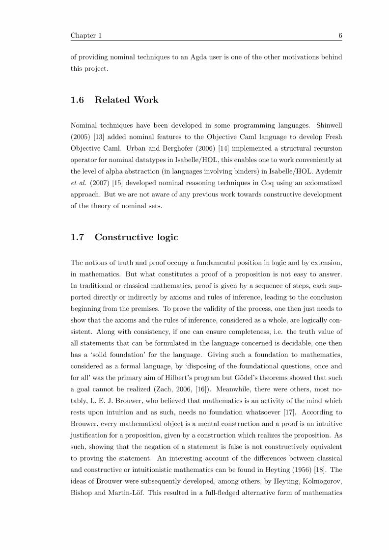
1.6 Related Work
Nominal techniques have been developed in some programming languages. Shinwell
(2005) [13] added nominal features to the Objective Caml language to develop Fresh
Objective Caml. Urban and Berghofer (2006) [14] implemented a structural recursion
operator for nominal datatypes in Isabelle/HOL, this enables one to work conveniently at
the level of alpha abstraction (in languages involving binders) in Isabelle/HOL. Aydemir
et al. (2007) [15] developed nominal reasoning techniques in Coq using an axiomatized
approach. But we are not aware of any previous work towards constructive development
of the theory of nominal sets.
1.7 Constructive logic
The notions of truth and proof occupy a fundamental position in logic and by extension,
in mathematics. But what constitutes a proof of a proposition is not easy to answer.
In traditional or classical mathematics, proof is given by a sequence of steps, each sup-
ported directly or indirectly by axioms and rules of inference, leading to the conclusion
beginning from the premises. To prove the validity of the process, one then just needs to
show that the axioms and the rules of inference, considered as a whole, are logically con-
sistent. Along with consistency, if one can ensure completeness, i.e. the truth value of
all statements that can be formulated in the language concerned is decidable, one then
has a ‘solid foundation’ for the language. Giving such a foundation to mathematics,
considered as a formal language, by ‘disposing of the foundational questions, once and
for all’ was the primary aim of Hilbert’s program but Godel’s theorems showed that such
a goal cannot be realized (Zach, 2006, [16]). Meanwhile, there were others, most no-
tably, L. E. J. Brouwer, who believed that mathematics is an activity of the mind which
rests upon intuition and as such, needs no foundation whatsoever [17]. According to
Brouwer, every mathematical object is a mental construction and a proof is an intuitive
justification for a proposition, given by a construction which realizes the proposition. As
such, showing that the negation of a statement is false is not constructively equivalent
to proving the statement. An interesting account of the differences between classical
and constructive or intuitionistic mathematics can be found in Heyting (1956) [18]. The
ideas of Brouwer were subsequently developed, among others, by Heyting, Kolmogorov,
Bishop and Martin-Lof. This resulted in a full-fledged alternative form of mathematics
Chapter 1 7
and logic, known as constructive mathematics and logic. One of the great advantages of
constructive logic is that it lends itself easily to machine level formalizations. As Martin-
Lof (1985) [19] puts it, ‘If programming is understood not as the writing of instructions
for this or that computing machine but as the design of methods of computation that
it is the computer’s duty to execute, then it no longer seems possible to distinguish the
discipline of programming from constructive mathematics’. It is precisely because of this
reason that Martin-Lof’s intuitionistic theory of types (1971) [20], originally developed
to formalize constructive mathematics, may well be viewed as a programming language.
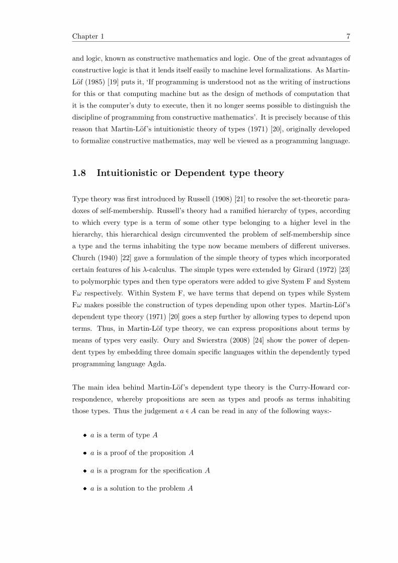
1.8 Intuitionistic or Dependent type theory
Type theory was first introduced by Russell (1908) [21] to resolve the set-theoretic para-
doxes of self-membership. Russell’s theory had a ramified hierarchy of types, according
to which every type is a term of some other type belonging to a higher level in the
hierarchy, this hierarchical design circumvented the problem of self-membership since
a type and the terms inhabiting the type now became members of different universes.
Church (1940) [22] gave a formulation of the simple theory of types which incorporated
certain features of his λ-calculus. The simple types were extended by Girard (1972) [23]
to polymorphic types and then type operators were added to give System F and System
Fω respectively. Within System F, we have terms that depend on types while System
Fω makes possible the construction of types depending upon other types. Martin-Lof’s
dependent type theory (1971) [20] goes a step further by allowing types to depend upon
terms. Thus, in Martin-Lof type theory, we can express propositions about terms by
means of types very easily. Oury and Swierstra (2008) [24] show the power of depen-
dent types by embedding three domain specific languages within the dependently typed
programming language Agda.
The main idea behind Martin-Lof’s dependent type theory is the Curry-Howard cor-
respondence, whereby propositions are seen as types and proofs as terms inhabiting
those types. Thus the judgement a ∈ A can be read in any of the following ways:-
� a is a term of type A
� a is a proof of the proposition A
� a is a program for the specification A
� a is a solution to the problem A
Chapter 1 8
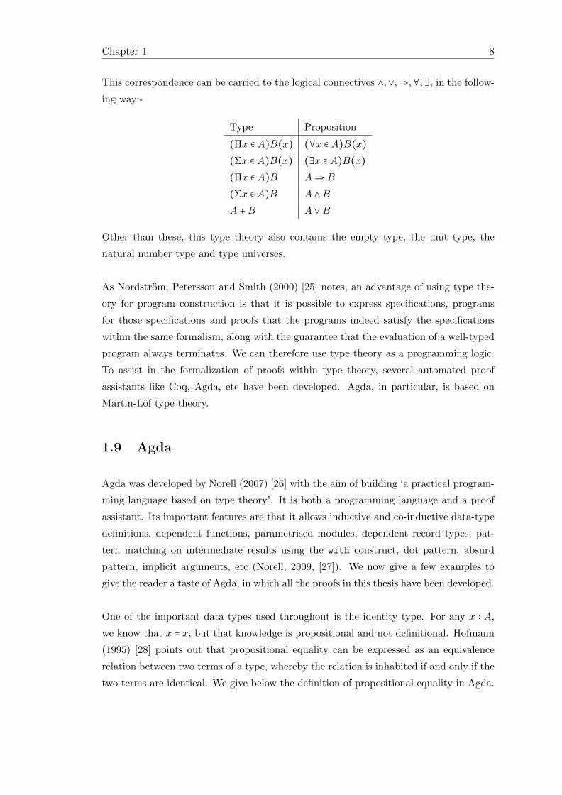
This correspondence can be carried to the logical connectives ∧,∨,⇒,∀,∃, in the follow-
ing way:-
Type Proposition
(Πx ∈ A)B(x) (∀x ∈ A)B(x)
(Σx ∈ A)B(x) (∃x ∈ A)B(x)
(Πx ∈ A)B A⇒ B
(Σx ∈ A)B A ∧B
A +B A ∨B
Other than these, this type theory also contains the empty type, the unit type, the
natural number type and type universes.
As Nordstrom, Petersson and Smith (2000) [25] notes, an advantage of using type the-
ory for program construction is that it is possible to express specifications, programs
for those specifications and proofs that the programs indeed satisfy the specifications
within the same formalism, along with the guarantee that the evaluation of a well-typed
program always terminates. We can therefore use type theory as a programming logic.
To assist in the formalization of proofs within type theory, several automated proof
assistants like Coq, Agda, etc have been developed. Agda, in particular, is based on
Martin-Lof type theory.
1.9 Agda
Agda was developed by Norell (2007) [26] with the aim of building ‘a practical program-
ming language based on type theory’. It is both a programming language and a proof
assistant. Its important features are that it allows inductive and co-inductive data-type
definitions, dependent functions, parametrised modules, dependent record types, pat-
tern matching on intermediate results using the with construct, dot pattern, absurd
pattern, implicit arguments, etc (Norell, 2009, [27]). We now give a few examples to
give the reader a taste of Agda, in which all the proofs in this thesis have been developed.
One of the important data types used throughout is the identity type. For any x ∶ A,
we know that x = x, but that knowledge is propositional and not definitional. Hofmann
(1995) [28] points out that propositional equality can be expressed as an equivalence
relation between two terms of a type, whereby the relation is inhabited if and only if the
two terms are identical. We give below the definition of propositional equality in Agda.
Chapter 1 9
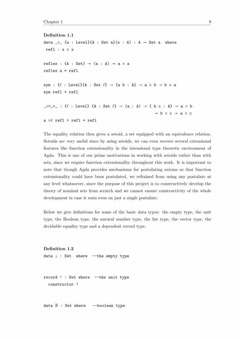
Definition 1.1
data _≡_ {a : Level}{A : Set a}(x : A) : A → Set a where
refl : x ≡ x
reflex : {A : Set} → (a : A) → a ≡ a
reflex a = refl
sym : {` : Level}{A : Set `} → {a b : A} → a ≡ b → b ≡ a
sym refl = refl
_≡<_>_ : {` : Level} {A : Set `} → (a : A) → { b c : A} → a ≡ b
→ b ≡ c → a ≡ c
a ≡< refl > refl = refl
The equality relation then gives a setoid, a set equipped with an equivalence relation.
Setoids are very useful since by using setoids, we can even recover several extensional
features like function extensionality in the intensional type theoretic environment of
Agda. This is one of our prime motivations in working with setoids rather than with
sets, since we require function extensionality throughout this work. It is important to
note that though Agda provides mechanisms for postulating axioms so that function
extensionality could have been postulated, we refrained from using any postulate at
any level whatsoever, since the purpose of this project is to constructively develop the
theory of nominal sets from scratch and we cannot ensure constructivity of the whole
development in case it rests even on just a single postulate.
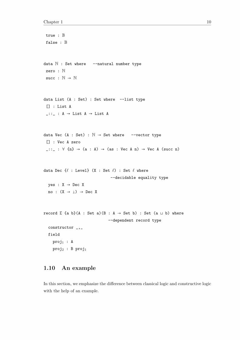
Below we give definitions for some of the basic data types: the empty type, the unit
type, the Boolean type, the natural number type, the list type, the vector type, the
decidable equality type and a dependent record type.
Definition 1.2
data � : Set where --the empty type
record ⊺ : Set where --the unit type
constructor 1
data B : Set where --boolean type
Chapter 1 10
true : Bfalse : B
data N : Set where --natural number type
zero : Nsucc : N → N
data List (A : Set) : Set where --list type
[] : List A
_::_ : A → List A → List A
data Vec (A : Set) : N → Set where --vector type
[] : Vec A zero
_::_ : ∀ {n} → (a : A) → (as : Vec A n) → Vec A (succ n)
data Dec {` : Level} (X : Set `) : Set ` where
--decidable equality type
yes : X → Dec X
no : (X → �) → Dec X
record Σ {a b}(A : Set a)(B : A → Set b) : Set (a ⊔ b) where
--dependent record type
constructor _,_
field
proj1 : A
proj2 : B proj1
1.10 An example
In this section, we emphasize the difference between classical logic and constructive logic
with the help of an example.
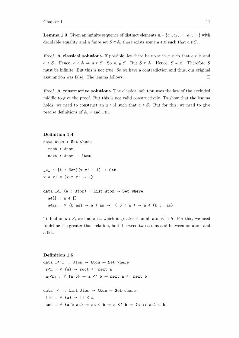
Chapter 1 11
Lemma 1.3 Given an infinite sequence of distinct elements A = {a0, a1, . . . , an, . . .} with
decidable equality and a finite set S ⊂ A, there exists some a ∈ A such that a ∉ S.
Proof. A classical solution:- If possible, let there be no such a such that a ∈ A and
a ∉ S. Hence, a ∈ A ⇒ a ∈ S. So A ⊆ S. But S ⊂ A. Hence, S = A. Therefore S
must be infinite. But this is not true. So we have a contradiction and thus, our original
assumption was false. The lemma follows.
Proof. A constructive solution:- The classical solution uses the law of the excluded
middle to give the proof. But this is not valid constructively. To show that the lemma
holds, we need to construct an a ∈ A such that a ∉ S. But for this, we need to give
precise definitions of A, ≠ and ∉ .
Definition 1.4
data Atom : Set where
root : Atom
next : Atom → Atom
_≠_ : {A : Set}(x x’ : A) → Set
x ≠ x’ = (x ≡ x’ → �)
data _∉_ (a : Atom) : List Atom → Set where
a∉[] : a ∉ []
a∉as : ∀ {b as} → a ∉ as → ( b ≠ a ) → a ∉ (b :: as)
To find an a ∉ S, we find an a which is greater than all atoms in S. For this, we need
to define the greater than relation, both between two atoms and between an atom and
a list.
Definition 1.5
data _<’_ : Atom → Atom → Set where
r<n : ∀ {a} → root <’ next a
n1<n2 : ∀ {a b} → a <’ b → next a <’ next b
data _<_ : List Atom → Atom → Set where
[]< : ∀ {a} → [] < a
as< : ∀ {a b as} → as < b → a <’ b → (a :: as) < b
Chapter 1 12
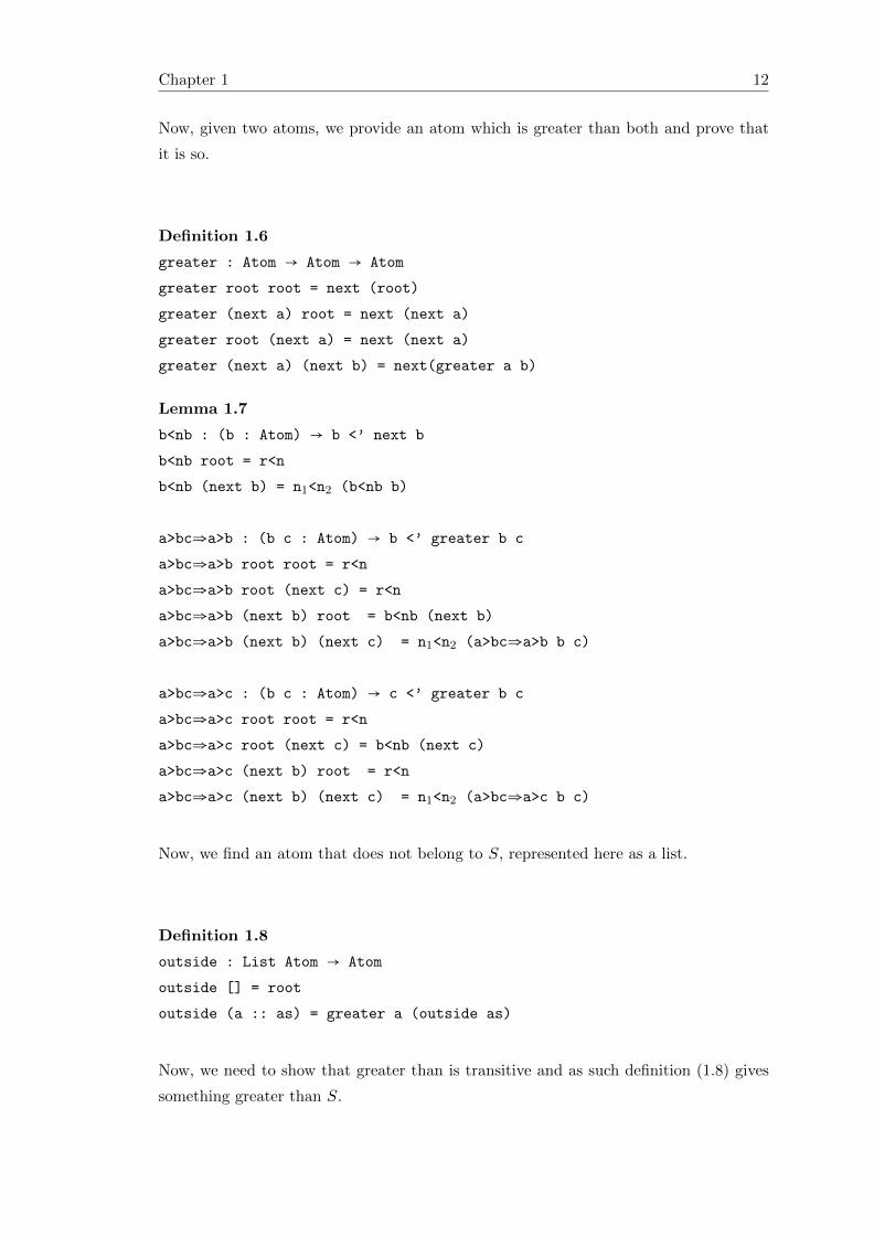
Now, given two atoms, we provide an atom which is greater than both and prove that
it is so.
Definition 1.6
greater : Atom → Atom → Atom
greater root root = next (root)
greater (next a) root = next (next a)
greater root (next a) = next (next a)
greater (next a) (next b) = next(greater a b)
Lemma 1.7
b<nb : (b : Atom) → b <’ next b
b<nb root = r<n
b<nb (next b) = n1<n2 (b<nb b)
a>bc⇒a>b : (b c : Atom) → b <’ greater b c
a>bc⇒a>b root root = r<n
a>bc⇒a>b root (next c) = r<n
a>bc⇒a>b (next b) root = b<nb (next b)
a>bc⇒a>b (next b) (next c) = n1<n2 (a>bc⇒a>b b c)
a>bc⇒a>c : (b c : Atom) → c <’ greater b c
a>bc⇒a>c root root = r<n
a>bc⇒a>c root (next c) = b<nb (next c)
a>bc⇒a>c (next b) root = r<n
a>bc⇒a>c (next b) (next c) = n1<n2 (a>bc⇒a>c b c)
Now, we find an atom that does not belong to S, represented here as a list.
Definition 1.8
outside : List Atom → Atom
outside [] = root
outside (a :: as) = greater a (outside as)
Now, we need to show that greater than is transitive and as such definition (1.8) gives
something greater than S.
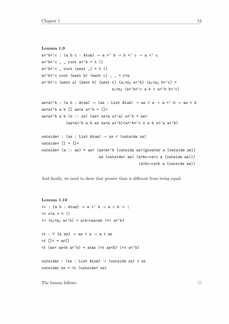
Chapter 1 13
Lemma 1.9
a<’b<’c : (a b c : Atom) → a <’ b → b <’ c → a <’ c
a<’b<’c _ _ root a<’b = λ ()
a<’b<’c _ root (next _) = λ ()
a<’b<’c root (next b) (next c) _ _ = r<n
a<’b<’c (next a) (next b) (next c) (n1<n2 a<’b) (n1<n2 b<’c) =
n1<n2 (a<’b<’c a b c a<’b b<’c)
as<a<’b : (a b : Atom) → (as : List Atom) → as < a → a <’ b → as < b
as<a<’b a b [] as<a a<’b = []<
as<a<’b a b (x :: xs) (as< xs<a x<’a) a<’b = as<
(as<a<’b a b xs xs<a a<’b)(a<’b<’c x a b x<’a a<’b)
outside< : (xs : List Atom) → xs < (outside xs)
outside< [] = []<
outside< (a :: as) = as< (as<a<’b (outside as)(greater a (outside as))
as (outside< as) (a>bc⇒a>c a (outside as)))
(a>bc⇒a>b a (outside as))
And finally, we need to show that greater than is different from being equal.
Lemma 1.10
<≠ : {a b : Atom} → a <’ b → a ≡ b → �
<≠ r<n = λ ()
<≠ (n1<n2 a<’b) = a≠b⇒na≠nb (<≠ a<’b)
<∉ : ∀ {a as} → as < a → a ∉ as
<∉ []< = a∉[]
<∉ (as< as<b a<’b) = a∉as (<∉ as<b) (<≠ a<’b)
outside∉ : (xs : List Atom) → (outside xs) ∉ xs
outside∉ xs = <∉ (outside< xs)
The lemma follows.
Chapter 1 14
This example shows two things. First, the constructive solution to a problem is not
always the same as the classical one. Secondly, in Agda, we need to work out everything
in explicit detail so much so that even re-bracketing of terms needs a justification in
terms of an explicit mention of the associativity of the operator concerned.
So in the following chapters, we skip some of the steps in our proofs for
brevity, steps without which our Agda programs won’t run but which oth-
erwise are fairly clear to any reader. In case of any doubt, the reader may
please refer to the program corresponding to the specification concerned.
1.11 Structure of the thesis
Chapter 2 discusses permutations, permutation actions, equivariant functions and prop-
erties of permutations. Chapter 3 gives a category theoretic treatment to nominal sets.
Chapter 4 develops properties of the freshness relation. Chapter 5 introduces name
abstraction sets and formalizes their properties. Chapter 6 concludes the dissertation.

Chapter 2
Permutations
One of the central ideas of the theory of nominal sets is that of finite permutations
and permutation actions. Given any set X, finite or infinite, we can define a finite
permutation P on X as a bijective function from X to X such that X ′ = {x ∣ P (x) ≠
x} ⊂X is finite. The set of all permutations, finite or infinite, on a set X form a group,
known as the symmetric group on X. The set of finite permutations is a subgroup of the
symmetric group. A finite permutation can also be represented by cycles, for example,
for the set X = {1,2,3,4}, the permutation P (1) = 1, P (2) = 3, P (3) = 4, P (4) = 2 can be
represented as (2 3 4), meaning 2→ 3→ 4→ 2. The representation by means of cycles
is not unique, since we can also represent P as (2 3)(2 4) meaning 2 → 3,3 → 2 →
4,4 → 2, i.e. the action is given by the composition of actions acting from left to right.
Now, if we wish to represent P by means of 2-cycles only, even then we cannot ensure a
unique representation since P can also be represented as (1 4)(2 3)(1 4)(2 4). We
shall have to accommodate this fact while defining permutations. In case of nominal
sets, finite permutations are nothing but bijective functions from a countably infinite
set of atomic names or Atoms to itself.
2.1 Atoms
Atom (A), as defined in definition (1.4), is a countably infinite set of atomic names with
decidable equality, meaning given any two atoms a, a′ ∈ A, we can decide whether a = a′
or a ≠ a′. An atom does not contain any element and it is not empty either.
16
Chapter 2 17
2.2 Finite permutations
A finite permutation can be defined as a list of pairs of atoms, i.e. as a list of 2-cycles.
Definition 2.1
Perm = List (Atom × Atom)
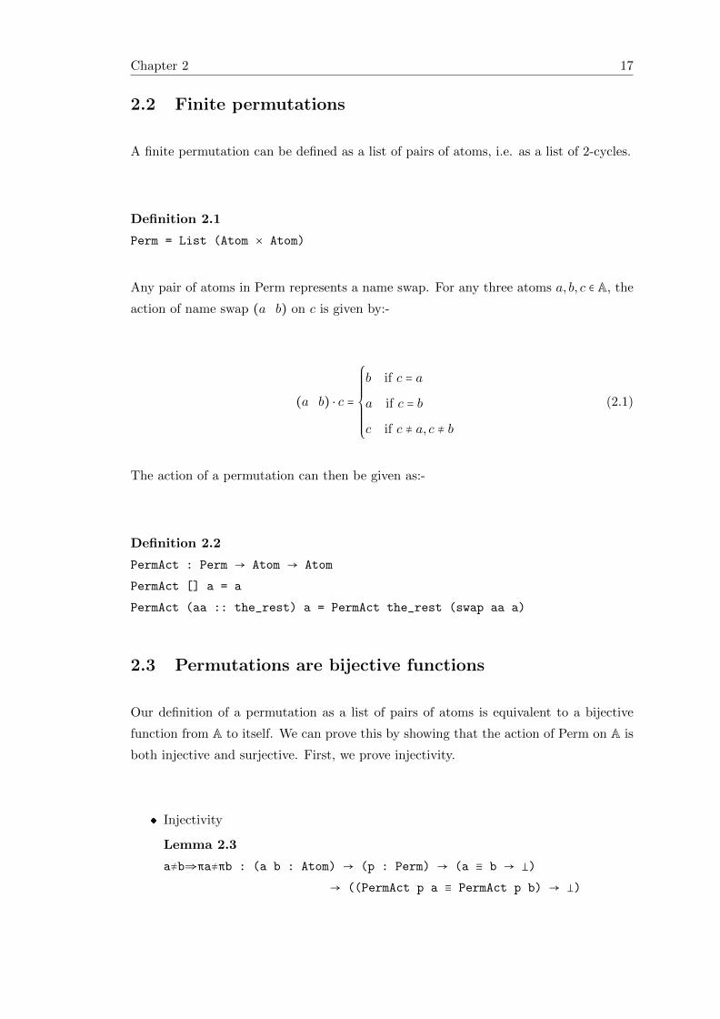
Any pair of atoms in Perm represents a name swap. For any three atoms a, b, c ∈ A, the
action of name swap (a b) on c is given by:-
(a b) ⋅ c =
⎧⎪⎪⎪⎪⎪⎪⎪⎨⎪⎪⎪⎪⎪⎪⎪⎩
b if c = a
a if c = b
c if c ≠ a, c ≠ b
(2.1)
The action of a permutation can then be given as:-
Definition 2.2
PermAct : Perm → Atom → Atom
PermAct [] a = a
PermAct (aa :: the_rest) a = PermAct the_rest (swap aa a)
2.3 Permutations are bijective functions
Our definition of a permutation as a list of pairs of atoms is equivalent to a bijective
function from A to itself. We can prove this by showing that the action of Perm on A is
both injective and surjective. First, we prove injectivity.
� Injectivity
Lemma 2.3
a≠b⇒πa≠πb : (a b : Atom) → (p : Perm) → (a ≡ b → �)
→ ((PermAct p a ≡ PermAct p b) → �)
Chapter 2 18
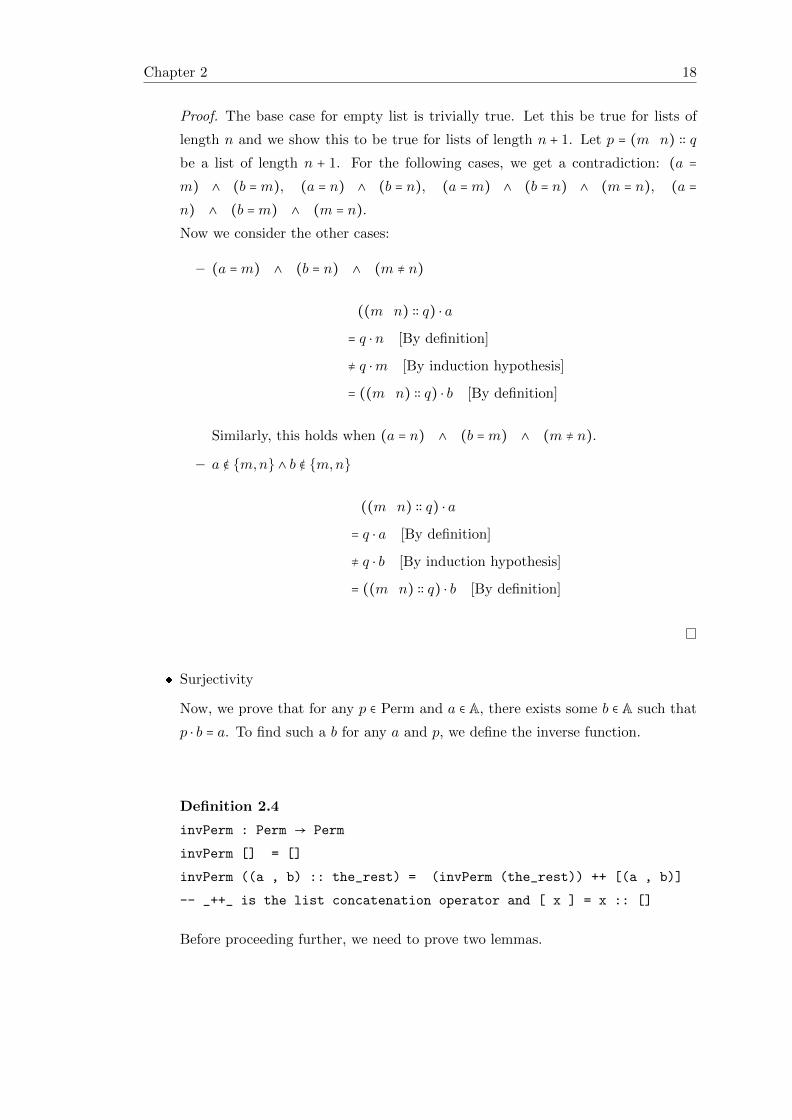
Proof. The base case for empty list is trivially true. Let this be true for lists of
length n and we show this to be true for lists of length n + 1. Let p = (m n) ∶∶ q
be a list of length n + 1. For the following cases, we get a contradiction: (a =
m) ∧ (b =m), (a = n) ∧ (b = n), (a =m) ∧ (b = n) ∧ (m = n), (a =
n) ∧ (b =m) ∧ (m = n).
Now we consider the other cases:
– (a =m) ∧ (b = n) ∧ (m ≠ n)
((m n) ∶∶ q) ⋅ a
= q ⋅ n [By definition]
≠ q ⋅m [By induction hypothesis]
= ((m n) ∶∶ q) ⋅ b [By definition]
Similarly, this holds when (a = n) ∧ (b =m) ∧ (m ≠ n).
– a ∉ {m,n} ∧ b ∉ {m,n}
((m n) ∶∶ q) ⋅ a
= q ⋅ a [By definition]
≠ q ⋅ b [By induction hypothesis]
= ((m n) ∶∶ q) ⋅ b [By definition]
� Surjectivity
Now, we prove that for any p ∈ Perm and a ∈ A, there exists some b ∈ A such that
p ⋅ b = a. To find such a b for any a and p, we define the inverse function.
Definition 2.4
invPerm : Perm → Perm
invPerm [] = []
invPerm ((a , b) :: the_rest) = (invPerm (the_rest)) ++ [(a , b)]
-- _++_ is the list concatenation operator and [ x ] = x :: []
Before proceeding further, we need to prove two lemmas.
Chapter 2 19
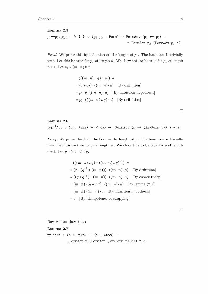
Lemma 2.5
p1++p2≡p2p1 : ∀ {a} → (p1 p2 : Perm) → PermAct (p1 ++ p2) a
≡ PermAct p2 (PermAct p1 a)
Proof. We prove this by induction on the length of p1. The base case is trivially
true. Let this be true for p1 of length n. We show this to be true for p1 of length
n + 1. Let p1 = (m n) ∶∶ q.
(((m n) ∶∶ q) + p2) ⋅ a
= (q + p2) ⋅ ((m n) ⋅ a) [By definition]
= p2 ⋅ q ⋅ ((m n) ⋅ a) [By induction hypothesis]
= p2 ⋅ (((m n) ∶∶ q) ⋅ a) [By definition]
Lemma 2.6
p○p-1Act : (p : Perm) → ∀ {a} → PermAct (p ++ (invPerm p)) a ≡ a
Proof. We prove this by induction on the length of p. The base case is trivially
true. Let this be true for p of length n. We show this to be true for p of length
n + 1. Let p = (m n) ∶∶ q.
(((m n) ∶∶ q) + ((m n) ∶∶ q)−1) ⋅ a
= (q + (q−1+ (m n))) ⋅ ((m n) ⋅ a) [By definition]
= ((q + q−1) + (m n)) ⋅ ((m n) ⋅ a) [By associativity]
= (m n) ⋅ (q + q−1) ⋅ ((m n) ⋅ a) [By lemma (2.5)]
= (m n) ⋅ (m n) ⋅ a [By induction hypothesis]
= a [By idempotence of swapping]
Now we can show that:
Lemma 2.7
pp-1a≡a : (p : Perm) → (a : Atom) →
(PermAct p (PermAct (invPerm p) a)) ≡ a
Chapter 2 20
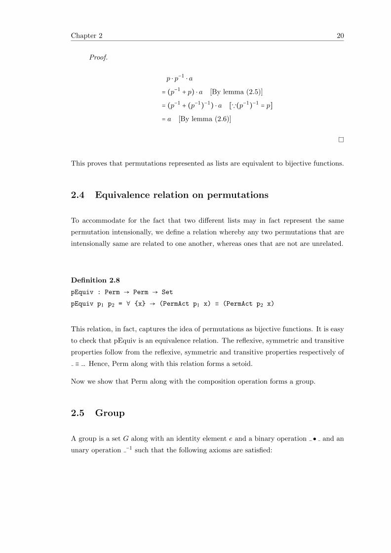
Proof.
p ⋅ p−1⋅ a
= (p−1+ p) ⋅ a [By lemma (2.5)]
= (p−1+ (p−1
)−1
) ⋅ a [∵(p−1)−1
= p]
= a [By lemma (2.6)]
This proves that permutations represented as lists are equivalent to bijective functions.
2.4 Equivalence relation on permutations
To accommodate for the fact that two different lists may in fact represent the same
permutation intensionally, we define a relation whereby any two permutations that are
intensionally same are related to one another, whereas ones that are not are unrelated.
Definition 2.8
pEquiv : Perm → Perm → Set
pEquiv p1 p2 = ∀ {x} → (PermAct p1 x) ≡ (PermAct p2 x)
This relation, in fact, captures the idea of permutations as bijective functions. It is easy
to check that pEquiv is an equivalence relation. The reflexive, symmetric and transitive
properties follow from the reflexive, symmetric and transitive properties respectively of
≡ . Hence, Perm along with this relation forms a setoid.
Now we show that Perm along with the composition operation forms a group.
2.5 Group
A group is a set G along with an identity element e and a binary operation ● and an
unary operation −1 such that the following axioms are satisfied:
Chapter 2 21
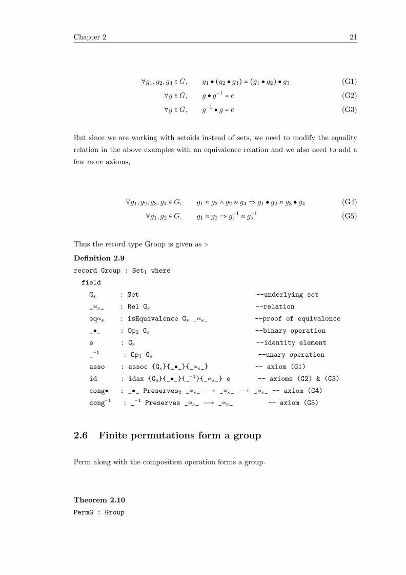
∀g1, g2, g3 ∈ G, g1 ● (g2 ● g3) = (g1 ● g2) ● g3 (G1)
∀g ∈ G, g ● g−1= e (G2)
∀g ∈ G, g−1● g = e (G3)
But since we are working with setoids instead of sets, we need to modify the equality
relation in the above examples with an equivalence relation and we also need to add a
few more axioms,
∀g1, g2, g3, g4 ∈ G, g1 ≈ g3 ∧ g2 ≈ g4 ⇒ g1 ● g2 ≈ g3 ● g4 (G4)
∀g1, g2 ∈ G, g1 ≈ g2 ⇒ g−11 ≈ g−1
2 (G5)
Thus the record type Group is given as :-
Definition 2.9
record Group : Set1 where
field
Gs : Set --underlying set
_≈s_ : Rel Gs --relation
eq≈s : isEquivalence Gs _≈s_ --proof of equivalence
_●_ : Op2 Gs --binary operation
e : Gs --identity element
_-1 : Op1 Gs --unary operation
asso : assoc {Gs}{_●_}{_≈s_} -- axiom (G1)
id : idax {Gs}{_●_}{_-1}{_≈s_} e -- axioms (G2) & (G3)
cong● : _●_ Preserves2 _≈s_ Ð→ _≈s_ Ð→ _≈s_ -- axiom (G4)
cong-1 : _-1 Preserves _≈s_ Ð→ _≈s_ -- axiom (G5)
2.6 Finite permutations form a group
Perm along with the composition operation forms a group.
Theorem 2.10
PermG : Group
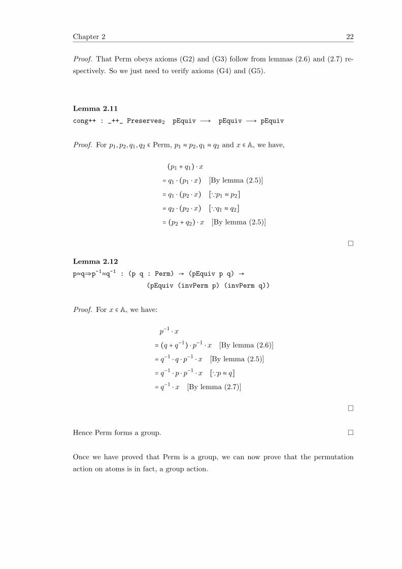
Chapter 2 22
Proof. That Perm obeys axioms (G2) and (G3) follow from lemmas (2.6) and (2.7) re-
spectively. So we just need to verify axioms (G4) and (G5).
Lemma 2.11
cong++ : _++_ Preserves2 pEquiv Ð→ pEquiv Ð→ pEquiv
Proof. For p1, p2, q1, q2 ∈ Perm, p1 ≈ p2, q1 ≈ q2 and x ∈ A, we have,
(p1 + q1) ⋅ x
= q1 ⋅ (p1 ⋅ x) [By lemma (2.5)]
= q1 ⋅ (p2 ⋅ x) [∵p1 ≈ p2]
= q2 ⋅ (p2 ⋅ x) [∵q1 ≈ q2]
= (p2 + q2) ⋅ x [By lemma (2.5)]
Lemma 2.12
p≈q⇒p-1≈q-1 : (p q : Perm) → (pEquiv p q) →
(pEquiv (invPerm p) (invPerm q))
Proof. For x ∈ A, we have:
p−1⋅ x
= (q + q−1) ⋅ p−1
⋅ x [By lemma (2.6)]
= q−1⋅ q ⋅ p−1
⋅ x [By lemma (2.5)]
= q−1⋅ p ⋅ p−1
⋅ x [∵p ≈ q]
= q−1⋅ x [By lemma (2.7)]
Hence Perm forms a group.
Once we have proved that Perm is a group, we can now prove that the permutation
action on atoms is in fact, a group action.
Chapter 2 23
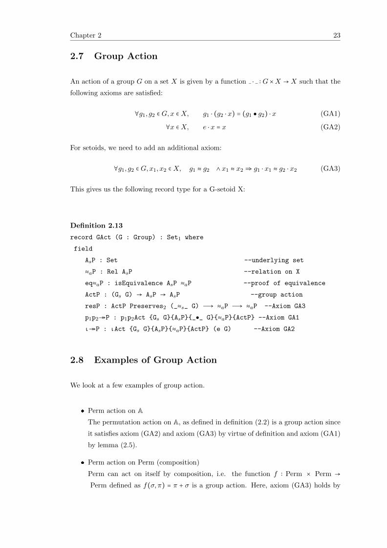
2.7 Group Action
An action of a group G on a set X is given by a function ⋅ ∶ G×X →X such that the
following axioms are satisfied:
∀g1, g2 ∈ G,x ∈X, g1 ⋅ (g2 ⋅ x) = (g1 ● g2) ⋅ x (GA1)
∀x ∈X, e ⋅ x = x (GA2)
For setoids, we need to add an additional axiom:
∀g1, g2 ∈ G,x1, x2 ∈X, g1 ≈ g2 ∧ x1 ≈ x2 ⇒ g1 ⋅ x1 ≈ g2 ⋅ x2 (GA3)
This gives us the following record type for a G-setoid X:
Definition 2.13
record GAct (G : Group) : Set1 where
field
AsP : Set --underlying set
≈aP : Rel AsP --relation on X
eq≈aP : isEquivalence AsP ≈aP --proof of equivalence
ActP : (Gs G) → AsP → AsP --group action
resP : ActP Preserves2 (_≈s_ G) Ð→ ≈aP Ð→ ≈aP --Axiom GA3
p1p2↠P : p1p2Act {Gs G}{AsP}{_●_ G}{≈aP}{ActP} --Axiom GA1
ι↠P : ιAct {Gs G}{AsP}{≈aP}{ActP} (e G) --Axiom GA2
2.8 Examples of Group Action
We look at a few examples of group action.
� Perm action on AThe permutation action on A, as defined in definition (2.2) is a group action since
it satisfies axiom (GA2) and axiom (GA3) by virtue of definition and axiom (GA1)
by lemma (2.5).
� Perm action on Perm (composition)
Perm can act on itself by composition, i.e. the function f ∶ Perm × Perm →
Perm defined as f(σ,π) = π + σ is a group action. Here, axiom (GA3) holds by
Chapter 2 24
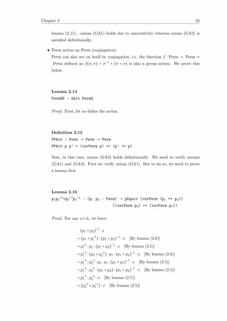
lemma (2.11) , axiom (GA1) holds due to associativity whereas axiom (GA2) is
satisfied definitionally.
� Perm action on Perm (conjugation)
Perm can also act on itself by conjugation, i.e. the function f ∶ Perm × Perm →
Perm defined as f(σ,π) = σ−1 + (π + σ) is also a group action. We prove this
below.
Lemma 2.14
PermGP : GAct PermG
Proof. First, let us define the action.
Definition 2.15
PPAct : Perm → Perm → Perm
PPAct p p’ = (invPerm p) ++ (p’ ++ p)
Now, in this case, axiom (GA2) holds definitionally. We need to verify axioms
(GA1) and (GA3). First we verify axiom (GA1). But to do so, we need to prove
a lemma first.
Lemma 2.16
p1p2-1≈p2
-1p1-1 : (p1 p2 : Perm) → pEquiv (invPerm (p1 ++ p2))
((invPerm p2) ++ (invPerm p1))
Proof. For any x ∈ A, we have:
(p1 + p2)−1⋅ x
= (p1 + p−11 ) ⋅ (p1 + p2)
−1⋅ x [By lemma (2.6)]
= p−11 ⋅ p1 ⋅ (p1 + p2)
−1⋅ x [By lemma (2.5)]
= p−11 ⋅ (p2 + p
−12 ) ⋅ p1 ⋅ (p1 + p2)
−1⋅ x [By lemma (2.6)]
= p−11 ⋅ p−1
2 ⋅ p2 ⋅ p1 ⋅ (p1 + p2)−1⋅ x [By lemma (2.5)]
= p−11 ⋅ p−1
2 ⋅ (p1 + p2) ⋅ (p1 + p2)−1⋅ x [By lemma (2.5)]
= p−11 ⋅ p−1
2 ⋅ x [By lemma (2.7)]
= (p−12 + p−1
1 ) ⋅ x [By lemma (2.5)]
Chapter 2 25
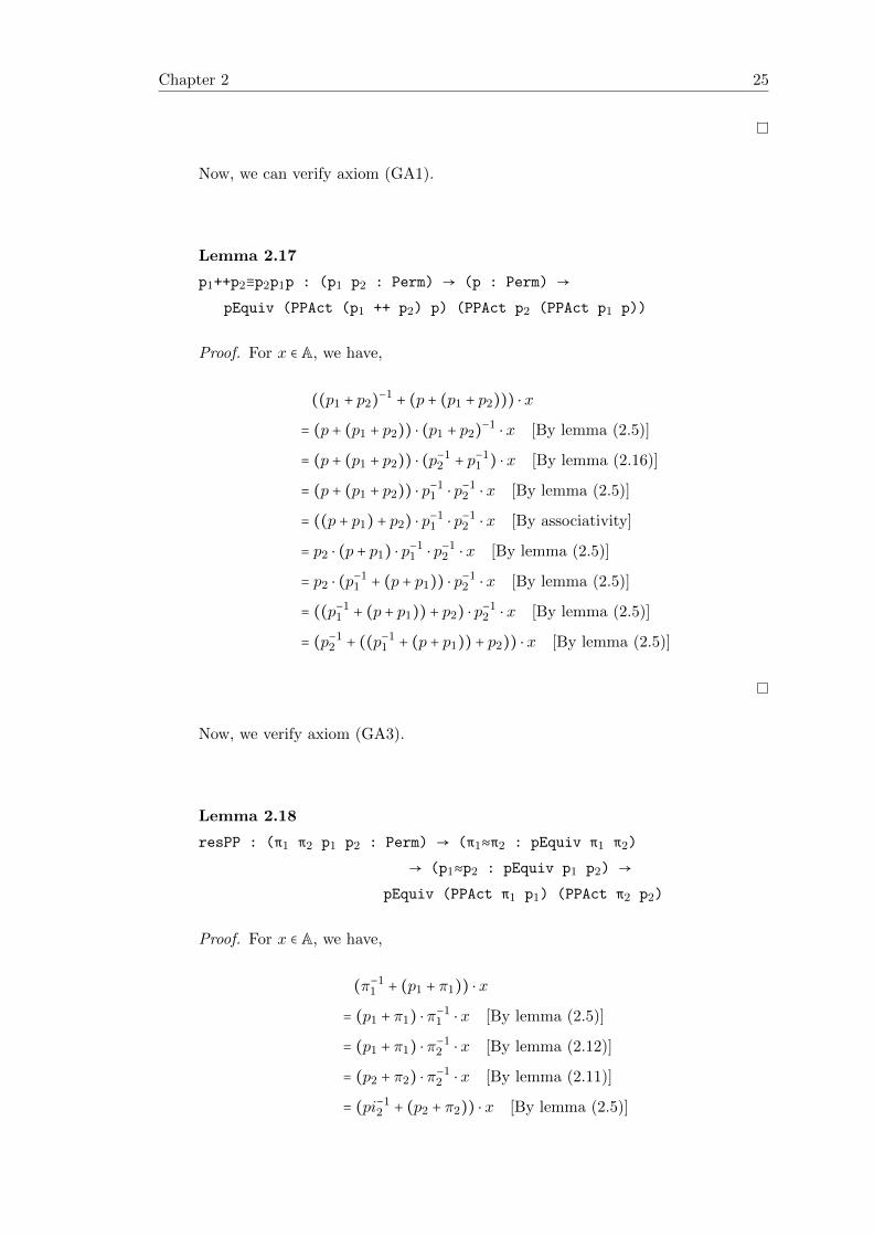
Now, we can verify axiom (GA1).
Lemma 2.17
p1++p2≡p2p1p : (p1 p2 : Perm) → (p : Perm) →
pEquiv (PPAct (p1 ++ p2) p) (PPAct p2 (PPAct p1 p))
Proof. For x ∈ A, we have,
((p1 + p2)−1+ (p + (p1 + p2))) ⋅ x
= (p + (p1 + p2)) ⋅ (p1 + p2)−1⋅ x [By lemma (2.5)]
= (p + (p1 + p2)) ⋅ (p−12 + p−1
1 ) ⋅ x [By lemma (2.16)]
= (p + (p1 + p2)) ⋅ p−11 ⋅ p−1
2 ⋅ x [By lemma (2.5)]
= ((p + p1) + p2) ⋅ p−11 ⋅ p−1
2 ⋅ x [By associativity]
= p2 ⋅ (p + p1) ⋅ p−11 ⋅ p−1
2 ⋅ x [By lemma (2.5)]
= p2 ⋅ (p−11 + (p + p1)) ⋅ p
−12 ⋅ x [By lemma (2.5)]
= ((p−11 + (p + p1)) + p2) ⋅ p
−12 ⋅ x [By lemma (2.5)]
= (p−12 + ((p−1
1 + (p + p1)) + p2)) ⋅ x [By lemma (2.5)]
Now, we verify axiom (GA3).
Lemma 2.18
resPP : (π1 π2 p1 p2 : Perm) → (π1≈π2 : pEquiv π1 π2)
→ (p1≈p2 : pEquiv p1 p2) →
pEquiv (PPAct π1 p1) (PPAct π2 p2)
Proof. For x ∈ A, we have,
(π−11 + (p1 + π1)) ⋅ x
= (p1 + π1) ⋅ π−11 ⋅ x [By lemma (2.5)]
= (p1 + π1) ⋅ π−12 ⋅ x [By lemma (2.12)]
= (p2 + π2) ⋅ π−12 ⋅ x [By lemma (2.11)]
= (pi−12 + (p2 + π2)) ⋅ x [By lemma (2.5)]
Chapter 2 26
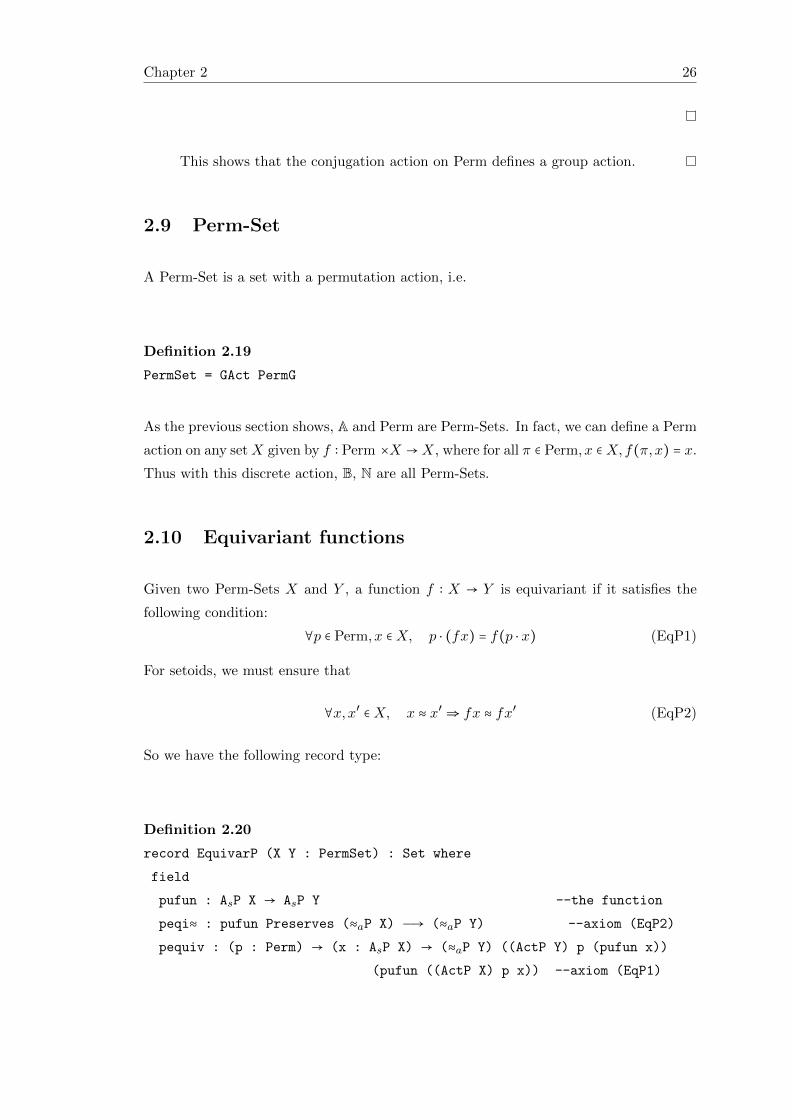
This shows that the conjugation action on Perm defines a group action.
2.9 Perm-Set
A Perm-Set is a set with a permutation action, i.e.
Definition 2.19
PermSet = GAct PermG
As the previous section shows, A and Perm are Perm-Sets. In fact, we can define a Perm
action on any setX given by f ∶ Perm ×X →X, where for all π ∈ Perm, x ∈X,f(π,x) = x.
Thus with this discrete action, B, N are all Perm-Sets.
2.10 Equivariant functions
Given two Perm-Sets X and Y , a function f ∶ X → Y is equivariant if it satisfies the
following condition:
∀p ∈ Perm, x ∈X, p ⋅ (fx) = f(p ⋅ x) (EqP1)
For setoids, we must ensure that
∀x,x′ ∈X, x ≈ x′ ⇒ fx ≈ fx′ (EqP2)
So we have the following record type:
Definition 2.20
record EquivarP (X Y : PermSet) : Set where
field
pufun : AsP X → AsP Y --the function
peqi≈ : pufun Preserves (≈aP X) Ð→ (≈aP Y) --axiom (EqP2)
pequiv : (p : Perm) → (x : AsP X) → (≈aP Y) ((ActP Y) p (pufun x))
(pufun ((ActP X) p x)) --axiom (EqP1)
Chapter 2 27
2.11 Example of an equivariant function
We look at an example of an equivariant function. The permutation action on any
Perm-Set X is itself an equivariant function, when the Perm action on Perm is defined
by conjugation. To see this, first we note that the cartesian product of two Perm-Sets is
again a Perm-Set, with the permutation action defined point-wise. Now, we prove that
the action indeed gives an equivariant function.
Lemma 2.21
GX→XEq : (X : PermSet) → EquivarP (ProdP PermGP X) X
--ProdP is the cartesian product function
Proof. Here, axiom (EqP2) holds due to axiom (GA3). We just need to verify ax-
iom (EqP1). For p ∈ Perm, (g, x) ∈ Perm ×X, we have,
p ⋅ g ⋅ x
= (g + p) ⋅ x [By Axiom (2.7)]
= (g + p) ⋅ e ⋅ x [By Axiom (2.8)]
= (g + p) ⋅ (p + p−1) ⋅ x [By lemma (2.6)]
= (g + p) ⋅ p−1⋅ p ⋅ x [By lemma (2.5)]
= (p−1+ (g + p)) ⋅ p ⋅ x [By lemma (2.5)]
= (p ⋅ g) ⋅ (p ⋅ x) [By definition]
2.12 Useful properties of permutations
We now state and prove a few properties of permutations which will be useful later.
2.12.1 Atoms unchanged under action
Since we are working with finite permutations, given any π ∈ Perm, we can always find
a ∈ A such that π ⋅ a = a. To find such an a, we observe that because of our definition
of Perm as lists of pairs of atoms, any a not present in π definitely remains unchanged
under the action of π. Put precisely,
Chapter 2 28
Definition 2.22
flatten : Perm → List Atom
flatten [] = []
flatten (p :: ps) = (proj1 p) :: ((proj2 p) :: (flatten ps))
Lemma 2.23
pa≡a : (p : Perm) → (a : Atom) → (a ∉ (flatten p)) → PermAct p a ≡ a
Proof. The base case for empty list is trivially true. Let this be true for lists of length
n. We show that this holds for lists of length n + 1. Let p = (m n) ∶∶ q. We have,
((m n) ∶∶ q) ⋅ a
= q ⋅ (m n) ⋅ a [By definition]
= q ⋅ a [∵a ≠m ∧ a ≠ n by definition (1.4)]
= a [By induction hypothesis]
2.12.2 A permutation and a name-swap
The composition of a permutation and a name-swap gives us the following useful lemma.
Lemma 2.24
π+πab≈abπ : (π : Perm) → (a b : Atom) →
pEquiv (π ++ [(PermAct π a) , (PermAct π b)]) ([(a , b)] ++ π)
Proof. For any x ∈ A, we have the following cases,
� x = a
(π + (π ⋅ a π ⋅ b)) ⋅ a
= (π ⋅ a π ⋅ b) ⋅ π ⋅ a [By lemma (2.5)]
= π ⋅ b [By definition]
= π ⋅ (a b) ⋅ a [By definition]
= ((a b) + π) ⋅ a [By lemma (2.5)]
Chapter 2 29
Similarly, we can show that the lemma holds for x = b.
� x ≠ a, x ≠ b
(π + (π ⋅ a π ⋅ b)) ⋅ x
= (π ⋅ a π ⋅ b) ⋅ π ⋅ x [By lemma (2.5)]
= π ⋅ x [∵π ⋅ x ≠ π ⋅ a, π ⋅ x ≠ π ⋅ b by lemma (2.3)]
= π ⋅ (a b) ⋅ x [By definition]
= ((a b) + π) ⋅ x [By lemma (2.5)]
Now, we have the following corollaries from the above lemma.
Corollary 2.25
πabπ≈πab : (π : Perm) → (a b : Atom) → (b ∉ (flatten π)) →
pEquiv (π ++ [((PermAct π a) , b)]) ([(a , b)] ++ π)
Proof. By lemma (2.24) and lemma (2.23).
Corollary 2.26
ab∉pcom : (a b : Atom) → (p : Perm) → (a ∉ (flatten p)) →
(b ∉ (flatten p)) → pEquiv ([( a , b )] ++ p) (p ++ [( a , b )])
Proof. By lemma (2.24) and lemma (2.23).
Corollary 2.27
πsuppAx : (p : Perm) → (b c : Atom) →
(b ∉ (flatten p)) → (c ∉ (flatten p)) → (a : Atom) →
PermAct ([( b , c)] ++ (p ++ [( b , c )])) a ≡ PermAct p a
Chapter 2 30
Proof. We have,
((b c) + (p + (b c))) ⋅ a
= ((b c) + ((b c) + p)) ⋅ a [By lemma (2.26)]
= (((b c) + (b c)) + p) ⋅ a [By associativity]
= p ⋅ a [By idempotence of swapping]
Corollary 2.28
ac≈ab+bc+ab : (a b c : Atom) → (c ≡ a → �) → (c ≡ b → �) →
pEquiv ([(a , c)]) ([(a , b)] ++ ([(b , c)] ++ [(a , b)]))
Proof. This can be easily seen to be true by a case analysis. We prove this in a different
way. For π ∈ Perm, a′, b′, x ∈ A, we have, by lemma (2.24),
(π + (π ⋅ a′ π ⋅ b′)) ⋅ π−1⋅ x = ((a′ b′) + π) ⋅ π−1
⋅ x
(π ⋅ a′ π ⋅ b′) ⋅ π ⋅ π−1x = (π−1+ ((a′ b′) + π)) ⋅ x [By lemma (2.5)]
(π ⋅ a′ π ⋅ b′) ⋅ x = (π−1+ ((a′ b′) + π)) ⋅ x [By lemma (2.7)]
Putting π = (a b), a′ = b, b′ = c, we have,
((a b) ⋅ b (a b) ⋅ c) ⋅ x = ((a b) + ((b c) + (a b))) ⋅ x
(a c)x = ((a b) + ((b c) + (a b))) ⋅ x [By definition]
We can now build the theory of nominal sets on top of the theory of permutations and
Perm-Sets.

Chapter 3
A category theoretic perspective
‘Just as group theory is the abstraction of the idea of a system of permutations of a set
or symmetries of an object’, category theory is the abstraction of the idea of functions
between mathematical objects. As the symmetries of an object abstractly characterize
it, the functions (or morphisms) of a category abstractly characterize the objects of the
category. Since functions are ubiquitous in mathematics, category theory ‘turns out to
be a kind of universal mathematical language like set theory’(Awodey, 2006, [29]). Ever
since its introduction by Eilenberg and Mac Lane (1945) [30], category theory has been
applied to many different fields of mathematics including geometry, algebra and logic.
In this chapter, we shall try to develop the theory of nominal sets in the language of
category theory.
3.1 Nominal Set
A Perm-Set X is a nominal set if every x ∈ X is finitely supported, i.e. given x ∈ X, we
can find a finite subset SX(x) ⊂ A such that for all π ∈ Perm,
((∀a ∈ SX(x)), π ⋅ a = a)⇒ π ⋅ x = x (S)
The support of an element is a set of names, each of which when remains unchanged by
a permutation, the element itself also remains unchanged. For example, the support of
an atomic name a ∈ A is any finite subset of A containing a. Thus, {a},{a, b},{a, b, c}
for b, c ∈ A are all supports for a. Classically, one can show that if SX(x) and S′X(x) are
finite supports for x ∈ X, then so is SX(x) ∩ S′X(x) (Proposition 2.3, [6]). As such, one
can work with a unique smallest support instead of any support. The smallest support
32
Chapter 3 33
can be defined as (Page 30, [6]):
suppXx ≜ ∩ {A ∈ Pow A ∣ A is a finite support for x} (SUPP)
where Pow A is the powerset of A. But as pointed out in section (1.4), we cannot find
suppXx constructively. So instead, we work with the notion of some non-unique finite
support (SX(x) ⊇ suppXx). Since SX(x) is an overestimate of the support for x, there
may be permutations π such that for all a ∈ SX(x), π ⋅ a = a does not hold, yet we have
π ⋅ x = x. But axiom (S) still holds true. Now, since we are working with permutations
represented as lists, we can express axiom (S) as:
∀b, c ∈ A, b ∉ SX(x) ∧ c ∉ SX(x)⇒ (b c) ⋅ x = x (N)
If b, c ∉ SX(x), then we know for sure that for all a ∈ SX(x), (b c) ⋅ a = a. By induction
then, it can be shown that for any π ∈ Perm, if (flatten π) ∩ SX(x) = ∅, then for all
a ∈ SX(x), π ⋅ a = a. So axiom (N) is equivalent to:
∀π ∈ Perm, (flatten π) ∩ SX(x) = ∅⇒ π ⋅ x = x (SSUPP)
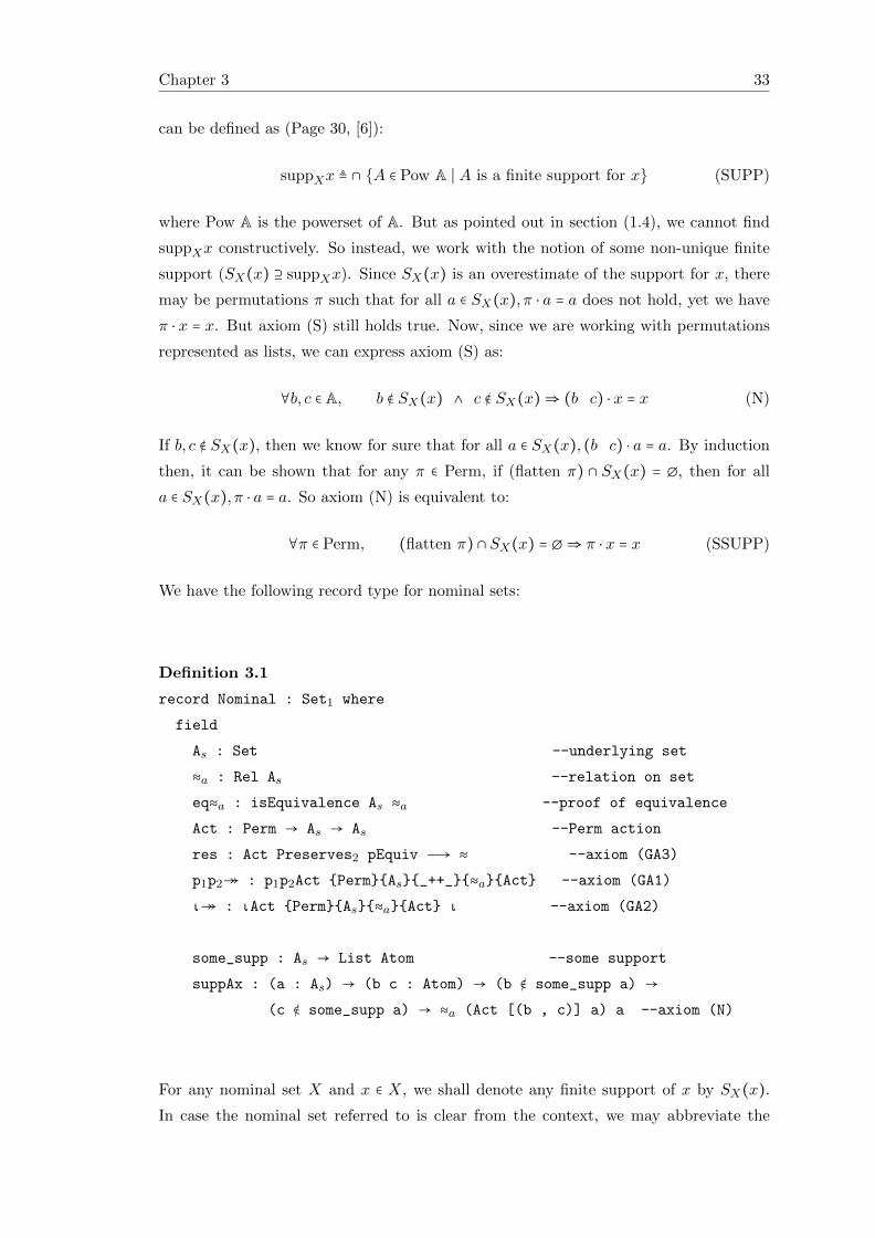
We have the following record type for nominal sets:
Definition 3.1
record Nominal : Set1 where
field
As : Set --underlying set
≈a : Rel As --relation on set
eq≈a : isEquivalence As ≈a --proof of equivalence
Act : Perm → As → As --Perm action
res : Act Preserves2 pEquiv Ð→ ≈ --axiom (GA3)
p1p2↠ : p1p2Act {Perm}{As}{_++_}{≈a}{Act} --axiom (GA1)
ι↠ : ιAct {Perm}{As}{≈a}{Act} ι --axiom (GA2)
some_supp : As → List Atom --some support
suppAx : (a : As) → (b c : Atom) → (b ∉ some_supp a) →
(c ∉ some_supp a) → ≈a (Act [(b , c)] a) a --axiom (N)
For any nominal set X and x ∈ X, we shall denote any finite support of x by SX(x).
In case the nominal set referred to is clear from the context, we may abbreviate the
Chapter 3 34
notation as S(x). Since we are working with some support, S(x) doesn’t refer to a
unique subset of A.
3.2 Examples of Nominal Sets
We now look at several examples of nominal sets.
� AA is a nominal set with SA(a) = {a}. That this satisfies axiom (N) follows by
definition.
� Perm (conjugation)
Perm with conjugation action is a nominal set with SPerm(π) = flatten π. That
this satisfies axiom (N) follows from corollary (2.27).
� Discrete Nominal Sets
B,N with the discrete action are nominal sets, where each element has an empty
support. Axiom (N) is satisfied trivially.
� Finite subsets of AWe can show that the set of finite subsets of any nominal set is also a nominal
set. Here, we show this for the nominal set A. For this, we represent a subset of Aas a list of atoms. Now if we define the setoid relation as the strict propositional
equality, then two equal subsets of A may be treated as different since lists may
contain multiple instances of the same element so that two lists may contain the
same set of elements but some of them occurring different number of times. In
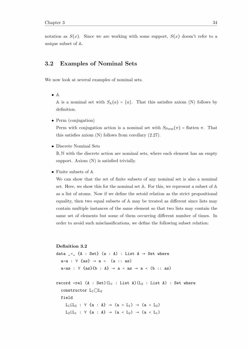
order to avoid such misclassifications, we define the following subset relation:
Definition 3.2
data _≺_ {A : Set} (a : A) : List A → Set where
a≺a : ∀ {as} → a ≺ (a :: as)
a≺as : ∀ {as}{b : A} → a ≺ as → a ≺ (b :: as)
record ≺rel (A : Set)(L1 : List A)(L2 : List A) : Set where
constructor L1◯L2
field
L1⊆L2 : ∀ {a : A} → (a ≺ L1) → (a ≺ L2)
L2⊆L1 : ∀ {a : A} → (a ≺ L2) → (a ≺ L1)
Chapter 3 35
Now, the equivalence property of the relation can be easily verified. With the
permutation action defined point-wise on each element of the list, we get a nominal
set where every list is supported by itself. That axioms (GA1), (GA2), (N) hold
follow from the corresponding properties of A. To verify axiom (GA3), we need
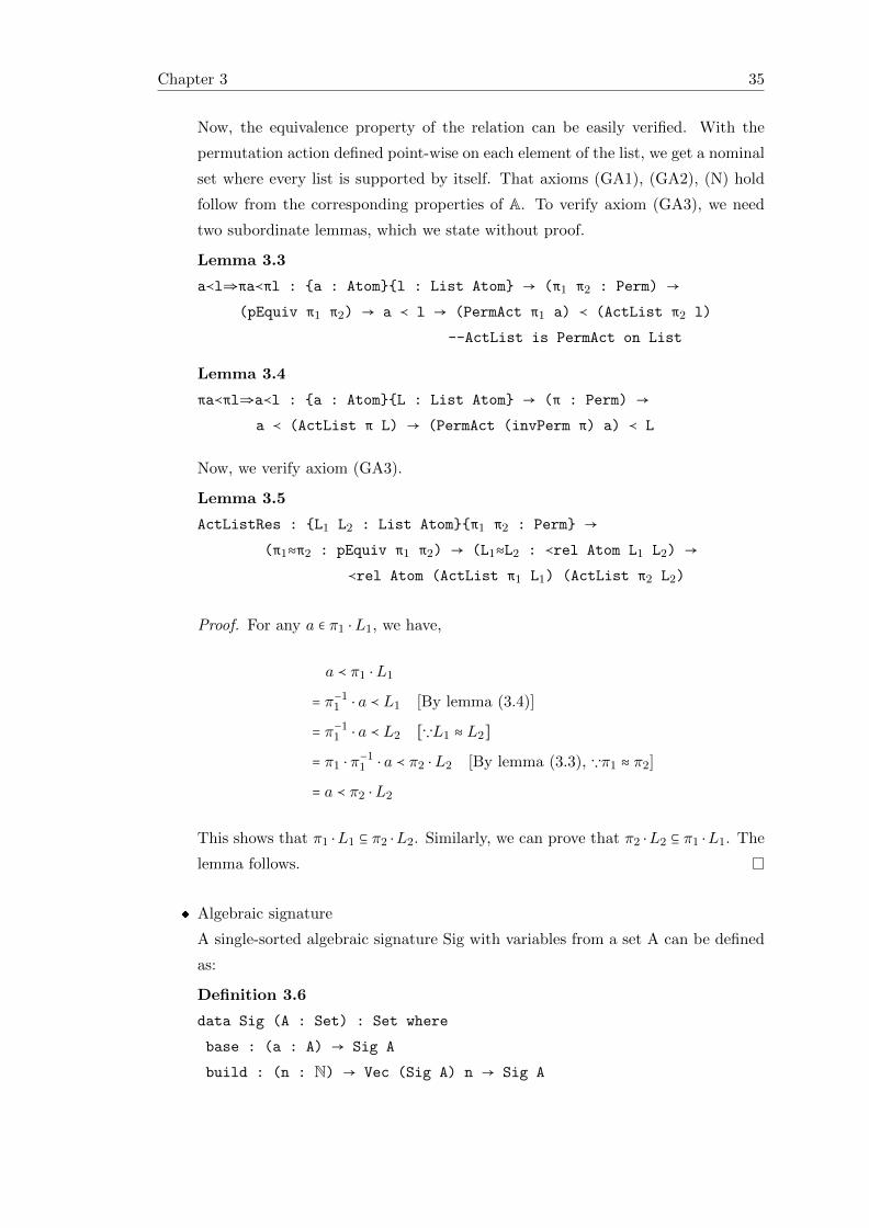
two subordinate lemmas, which we state without proof.
Lemma 3.3
a≺l⇒πa≺πl : {a : Atom}{l : List Atom} → (π1 π2 : Perm) →
(pEquiv π1 π2) → a ≺ l → (PermAct π1 a) ≺ (ActList π2 l)
--ActList is PermAct on List
Lemma 3.4
πa≺πl⇒a≺l : {a : Atom}{L : List Atom} → (π : Perm) →
a ≺ (ActList π L) → (PermAct (invPerm π) a) ≺ L
Now, we verify axiom (GA3).
Lemma 3.5
ActListRes : {L1 L2 : List Atom}{π1 π2 : Perm} →
(π1≈π2 : pEquiv π1 π2) → (L1≈L2 : ≺rel Atom L1 L2) →
≺rel Atom (ActList π1 L1) (ActList π2 L2)
Proof. For any a ∈ π1 ⋅L1, we have,
a ≺ π1 ⋅L1
= π−11 ⋅ a ≺ L1 [By lemma (3.4)]
= π−11 ⋅ a ≺ L2 [∵L1 ≈ L2]
= π1 ⋅ π−11 ⋅ a ≺ π2 ⋅L2 [By lemma (3.3), ∵π1 ≈ π2]
= a ≺ π2 ⋅L2
This shows that π1 ⋅L1 ⊆ π2 ⋅L2. Similarly, we can prove that π2 ⋅L2 ⊆ π1 ⋅L1. The
lemma follows.
� Algebraic signature
A single-sorted algebraic signature Sig with variables from a set A can be defined
as:
Definition 3.6
data Sig (A : Set) : Set where
base : (a : A) → Sig A
build : (n : N) → Vec (Sig A) n → Sig A
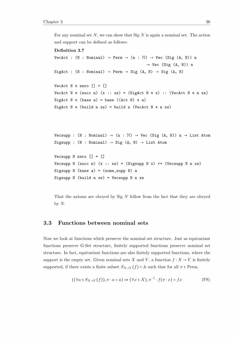
Chapter 3 36
For any nominal set N , we can show that Sig N is again a nominal set. The action
and support can be defined as follows:
Definition 3.7
VecAct : (N : Nominal) → Perm → (n : N) → Vec (Sig (As N)) n
→ Vec (Sig (As N)) n
SigAct : (N : Nominal) → Perm → Sig (As N) → Sig (As N)
VecAct N π zero [] = []
VecAct N π (succ n) (x :: xs) = (SigAct N π x) :: (VecAct N π n xs)
SigAct N π (base a) = base ((Act N) π a)
SigAct N π (build n xs) = build n (VecAct N π n xs)
Vecsupp : (N : Nominal) → (n : N) → Vec (Sig (As N)) n → List Atom
Sigsupp : (N : Nominal) → Sig (As N) → List Atom
Vecsupp N zero [] = []
Vecsupp N (succ n) (x :: xs) = (Sigsupp N x) ++ (Vecsupp N n xs)
Sigsupp N (base a) = (some_supp N) a
Sigsupp N (build n xs) = Vecsupp N n xs
That the axioms are obeyed by Sig N follow from the fact that they are obeyed
by N .
3.3 Functions between nominal sets
Now we look at functions which preserve the nominal set structure. Just as equivariant
functions preserve G-Set structure, finitely supported functions preserve nominal set
structure. In fact, equivariant functions are also finitely supported functions, where the
support is the empty set. Given nominal sets X and Y , a function f ∶X → Y is finitely
supported, if there exists a finite subset SX→Y (f) ⊂ A such that for all π ∈ Perm,
((∀a ∈ SX→Y (f)), π ⋅ a = a)⇒ (∀x ∈X), π−1⋅ f(π ⋅ x) = fx (FS)
Chapter 3 37
Here again, we shall work with some support instead of the smallest support. In line
with our definition for nominal set, we modify axiom (FS) as:
∀b, c ∈ A, b ∉ SX→Y (f), c ∉ SX→Y (f)⇒ (∀x ∈X), (b c) ⋅ f((b c) ⋅ x) = fx (FS1)
But since we are working with setoids, we need to add an additional axiom:
∀x1, x2 ∈X, x1 ≈ x2 ⇒ fx1 ≈ fx2 (FS2)
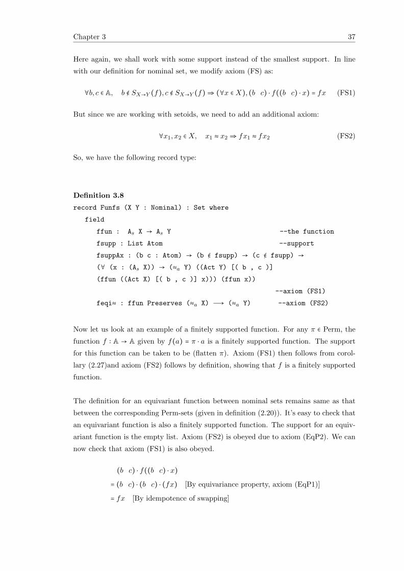
So, we have the following record type:
Definition 3.8
record Funfs (X Y : Nominal) : Set where
field
ffun : As X → As Y --the function
fsupp : List Atom --support
fsuppAx : (b c : Atom) → (b ∉ fsupp) → (c ∉ fsupp) →
(∀ (x : (As X)) → (≈a Y) ((Act Y) [( b , c )]
(ffun ((Act X) [( b , c )] x))) (ffun x))
--axiom (FS1)
feqi≈ : ffun Preserves (≈a X) Ð→ (≈a Y) --axiom (FS2)
Now let us look at an example of a finitely supported function. For any π ∈ Perm, the
function f ∶ A → A given by f(a) = π ⋅ a is a finitely supported function. The support
for this function can be taken to be (flatten π). Axiom (FS1) then follows from corol-
lary (2.27)and axiom (FS2) follows by definition, showing that f is a finitely supported
function.
The definition for an equivariant function between nominal sets remains same as that
between the corresponding Perm-sets (given in definition (2.20)). It’s easy to check that
an equivariant function is also a finitely supported function. The support for an equiv-
ariant function is the empty list. Axiom (FS2) is obeyed due to axiom (EqP2). We can
now check that axiom (FS1) is also obeyed.
(b c) ⋅ f((b c) ⋅ x)
= (b c) ⋅ (b c) ⋅ (fx) [By equivariance property, axiom (EqP1)]
= fx [By idempotence of swapping]
Chapter 3 38
Once we have got nominal sets and functions between nominal sets, we can now look at
the category of nominal sets.
3.4 Nom and Nomfs
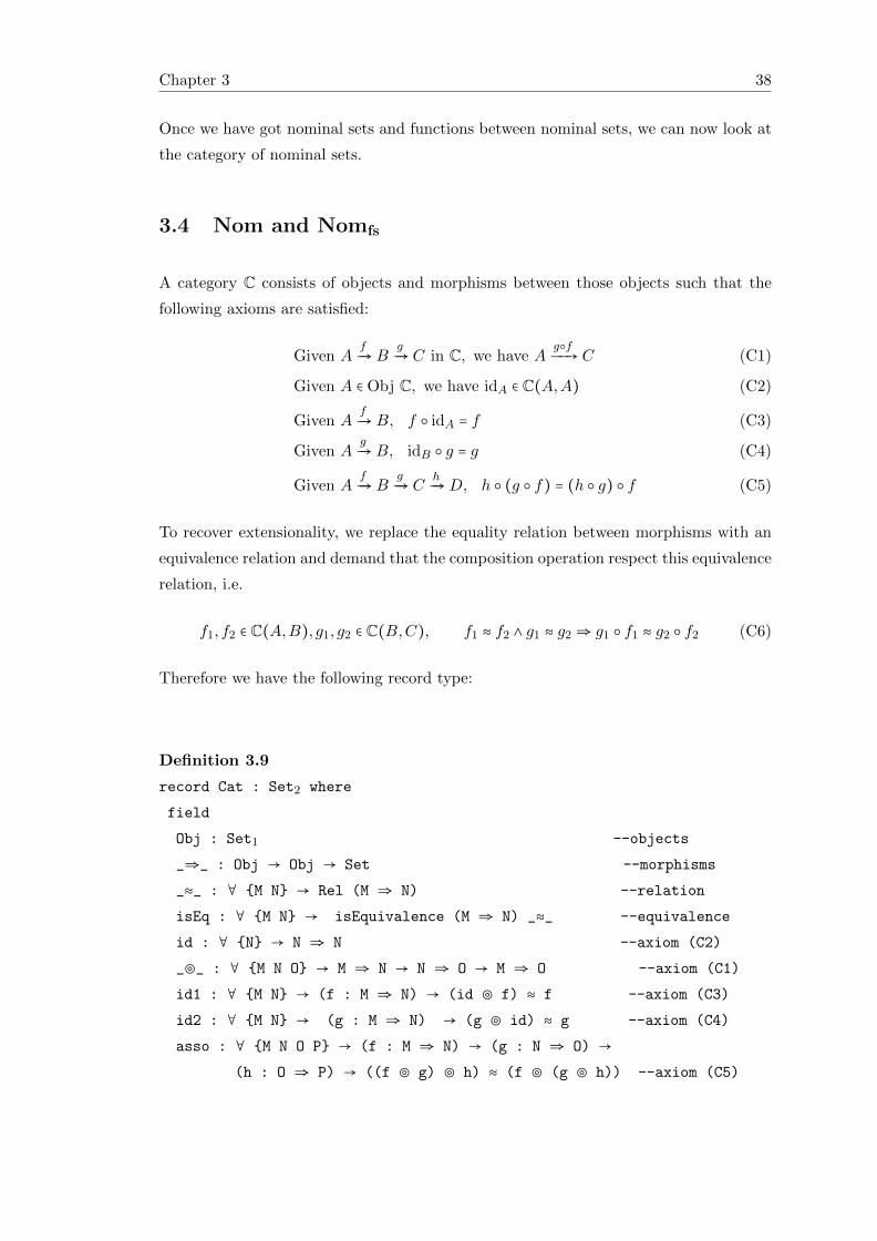
A category C consists of objects and morphisms between those objects such that the
following axioms are satisfied:
Given AfÐ→ B
gÐ→ C in C, we have A
g○fÐÐ→ C (C1)
Given A ∈ Obj C, we have idA ∈ C(A,A) (C2)
Given AfÐ→ B, f ○ idA = f (C3)
Given AgÐ→ B, idB ○ g = g (C4)
Given AfÐ→ B
gÐ→ C
hÐ→D, h ○ (g ○ f) = (h ○ g) ○ f (C5)
To recover extensionality, we replace the equality relation between morphisms with an
equivalence relation and demand that the composition operation respect this equivalence
relation, i.e.
f1, f2 ∈ C(A,B), g1, g2 ∈ C(B,C), f1 ≈ f2 ∧ g1 ≈ g2 ⇒ g1 ○ f1 ≈ g2 ○ f2 (C6)
Therefore we have the following record type:
Definition 3.9
record Cat : Set2 where
field
Obj : Set1 --objects
_⇒_ : Obj → Obj → Set --morphisms
_≈_ : ∀ {M N} → Rel (M ⇒ N) --relation
isEq : ∀ {M N} → isEquivalence (M ⇒ N) _≈_ --equivalence
id : ∀ {N} → N ⇒ N --axiom (C2)
_⊚_ : ∀ {M N O} → M ⇒ N → N ⇒ O → M ⇒ O --axiom (C1)
id1 : ∀ {M N} → (f : M ⇒ N) → (id ⊚ f) ≈ f --axiom (C3)
id2 : ∀ {M N} → (g : M ⇒ N) → (g ⊚ id) ≈ g --axiom (C4)
asso : ∀ {M N O P} → (f : M ⇒ N) → (g : N ⇒ O) →
(h : O ⇒ P) → ((f ⊚ g) ⊚ h) ≈ (f ⊚ (g ⊚ h)) --axiom (C5)
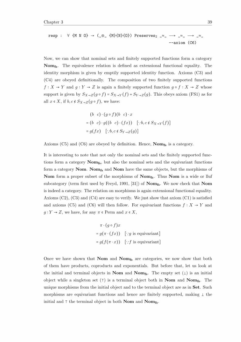
Chapter 3 39
resp : ∀ {M N O} → (_⊚_ {M}{N}{O}) Preserves2 _≈_ Ð→ _≈_ Ð→ _≈_
--axiom (C6)
Now, we can show that nominal sets and finitely supported functions form a category
Nomfs. The equivalence relation is defined as extensional functional equality. The
identity morphism is given by emptily supported identity function. Axioms (C3) and
(C4) are obeyed definitionally. The composition of two finitely supported functions
f ∶ X → Y and g ∶ Y → Z is again a finitely supported function g ○ f ∶ X → Z whose
support is given by SX→Z(g ○ f) = SX→Y (f) + SY→Z(g). This obeys axiom (FS1) as for
all x ∈X, if b, c ∉ SX→Z(g ○ f), we have:
(b c) ⋅ (g ○ f)(b c) ⋅ x
= (b c) ⋅ g((b c) ⋅ (fx)) [∵b, c ∉ SX→Y (f)]
= g(fx) [∵b, c ∉ SY→Z(g)]
Axioms (C5) and (C6) are obeyed by definition. Hence, Nomfs is a category.
It is interesting to note that not only the nominal sets and the finitely supported func-
tions form a category Nomfs, but also the nominal sets and the equivariant functions
form a category Nom. Nomfs and Nom have the same objects, but the morphisms of
Nom form a proper subset of the morphisms of Nomfs. Thus Nom is a wide or lluf
subcategory (term first used by Freyd, 1991, [31]) of Nomfs. We now check that Nom
is indeed a category. The relation on morphisms is again extensional functional equality.
Axioms (C2), (C3) and (C4) are easy to verify. We just show that axiom (C1) is satisfied
and axioms (C5) and (C6) will then follow. For equivariant functions f ∶ X → Y and
g ∶ Y → Z, we have, for any π ∈ Perm and x ∈X,
π ⋅ (g ○ f)x
= g(π ⋅ (fx)) [∵g is equivariant]
= g(f(π ⋅ x)) [∵f is equivariant]
Once we have shown that Nom and Nomfs are categories, we now show that both
of them have products, coproducts and exponentials. But before that, let us look at
the initial and terminal objects in Nom and Nomfs. The empty set (�) is an initial
object while a singleton set (⊺) is a terminal object both in Nom and Nomfs. The
unique morphisms from the initial object and to the terminal object are as in Set. Such
morphisms are equivariant functions and hence are finitely supported, making � the
initial and ⊺ the terminal object in both Nom and Nomfs.
Chapter 3 40
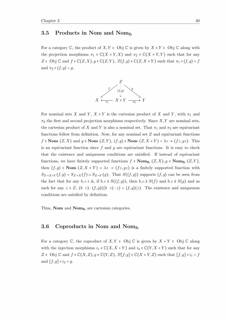
3.5 Products in Nom and Nomfs
For a category C, the product of X,Y ∈ Obj C is given by X × Y ∈ Obj C along with
the projection morphisms π1 ∈ C(X × Y,X) and π2 ∈ C(X × Y,Y ) such that for any
Z ∈ Obj C and f ∈ C(Z,X), g ∈ C(Z,Y ), ∃!⟨f, g⟩ ∈ C(Z,X × Y ) such that π1 ○ ⟨f, g⟩ = f
and π2 ○ ⟨f, g⟩ = g.
Z
X X × Y Y
f ⟨f,g⟩ g
π1 π2
For nominal sets X and Y , X × Y is the cartesian product of X and Y , with π1 and
π2 the first and second projection morphisms respectively. Since X,Y are nominal sets,
the cartesian product of X and Y is also a nominal set. That π1 and π2 are equivariant
functions follow from definition. Now, for any nominal set Z and equivariant functions
f ∈ Nom (Z,X) and g ∈ Nom (Z,Y ), ⟨f, g⟩ ∈ Nom (Z,X × Y ) = λz → (fz, gz). This
is an equivariant function since f and g are equivariant functions. It is easy to check
that the existence and uniqueness conditions are satisfied. If instead of equivariant
functions, we have finitely supported functions f ∈ Nomfs (Z,X), g ∈ Nomfs (Z,Y ),
then ⟨f, g⟩ ∈ Nom (Z,X × Y ) = λz → (fz, gz) is a finitely supported function with
SZ→X×Y ⟨f, g⟩ = SZ→X(f) ∪ SZ→Y (g). That S(⟨f, g⟩) supports ⟨f, g⟩ can be seen from
the fact that for any b, c ∈ A, if b, c ∉ S(⟨f, g⟩), then b, c ∉ S(f) and b, c ∉ S(g) and as
such for any z ∈ Z, (b c) ⋅ ⟨f, g⟩((b c) ⋅ z) = ⟨f, g⟩(z). The existence and uniqueness
conditions are satisfied by definition.
Thus, Nom and Nomfs are cartesian categories.
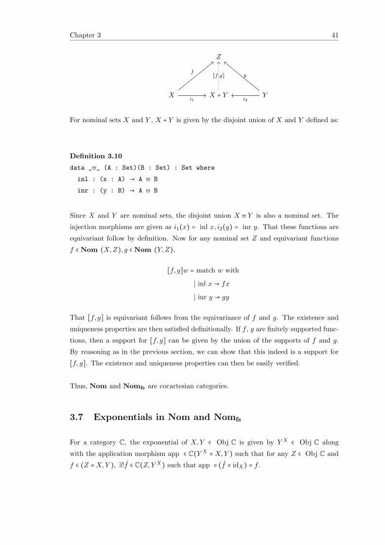
3.6 Coproducts in Nom and Nomfs
For a category C, the coproduct of X,Y ∈ Obj C is given by X + Y ∈ Obj C along
with the injection morphisms i1 ∈ C(X,X + Y ) and i2 ∈ C(Y,X + Y ) such that for any
Z ∈ Obj C and f ∈ C(X,Z), g ∈ C(Y,Z), ∃![f, g] ∈ C(X + Y,Z) such that [f, g] ○ i1 = f
and [f, g] ○ i2 = g.
Chapter 3 41
Z
X X + Y Y
f
i1
[f,g]
i2
g
For nominal sets X and Y , X + Y is given by the disjoint union of X and Y defined as:
Definition 3.10
data _⊎_ (A : Set)(B : Set) : Set where
inl : (x : A) → A ⊎ B
inr : (y : B) → A ⊎ B
Since X and Y are nominal sets, the disjoint union X ⊎ Y is also a nominal set. The
injection morphisms are given as i1(x) = inl x, i2(y) = inr y. That these functions are
equivariant follow by definition. Now for any nominal set Z and equivariant functions
f ∈ Nom (X,Z), g ∈ Nom (Y,Z),
[f, g]w = match w with
∣ inl x→ fx
∣ inr y → gy
That [f, g] is equivariant follows from the equivariance of f and g. The existence and
uniqueness properties are then satisfied definitionally. If f , g are finitely supported func-
tions, then a support for [f, g] can be given by the union of the supports of f and g.
By reasoning as in the previous section, we can show that this indeed is a support for
[f, g]. The existence and uniqueness properties can then be easily verified.
Thus, Nom and Nomfs are cocartesian categories.
3.7 Exponentials in Nom and Nomfs
For a category C, the exponential of X,Y ∈ Obj C is given by Y X ∈ Obj C along
with the application morphism app ∈ C(Y X ×X,Y ) such that for any Z ∈ Obj C and
f ∈ (Z ×X,Y ), ∃!f ∈ C(Z,Y X) such that app ○ (f × idX) = f .
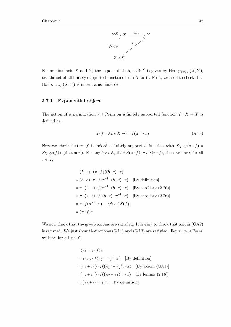
Chapter 3 42
Y X ×X Y
Z ×X
app
f×idX
f
For nominal sets X and Y , the exponential object Y X is given by HomNomfs(X,Y ),
i.e. the set of all finitely supported functions from X to Y . First, we need to check that
HomNomfs(X,Y ) is indeed a nominal set.
3.7.1 Exponential object
The action of a permutation π ∈ Perm on a finitely supported function f ∶ X → Y is
defined as:
π ⋅ f = λx ∈X → π ⋅ f(π−1⋅ x) (AFS)
Now we check that π ⋅ f is indeed a finitely supported function with SX→Y (π ⋅ f) =
SX→Y (f) ∪ (flatten π). For any b, c ∈ A, if b ∉ S(π ⋅ f), c ∉ S(π ⋅ f), then we have, for all
x ∈X,
(b c) ⋅ (π ⋅ f)((b c) ⋅ x)
= (b c) ⋅ π ⋅ f(π−1⋅ (b c) ⋅ x) [By definition]
= π ⋅ (b c) ⋅ f(π−1⋅ (b c) ⋅ x) [By corollary (2.26)]
= π ⋅ (b c) ⋅ f((b c) ⋅ π−1⋅ x) [By corollary (2.26)]
= π ⋅ f(π−1⋅ x) [∵b, c ∉ S(f)]
= (π ⋅ f)x
We now check that the group axioms are satisfied. It is easy to check that axiom (GA2)
is satisfied. We just show that axioms (GA1) and (GA3) are satisfied. For π1, π2 ∈ Perm,
we have for all x ∈X,
(π1 ⋅ π2 ⋅ f)x
= π1 ⋅ π2 ⋅ f(π−12 ⋅ π−1
1 ⋅ x) [By definition]
= (π2 + π1) ⋅ f((π−11 + π−1
2 ) ⋅ x) [By axiom (GA1)]
= (π2 + π1) ⋅ f((π2 + π1)−1⋅ x) [By lemma (2.16)]
= ((π2 + π1) ⋅ f)x [By definition]
Chapter 3 43
Now, for π1, π2 ∈ Perm and f1, f2 ∈ Nomfs (X,Y ), if π1 ≈ π2 and f1 ≈ f2, then we have,
for all x ∈X,
(π1 ⋅ f1)x
= π1 ⋅ f1(π−11 ⋅ x) [By definition]
= π1 ⋅ f1(π−12 ⋅ x) [By lemma (2.12), ∵π1 ≈ π2]
= π2 ⋅ f2(π−12 ⋅ x) [∵π1 ≈ π2, f1 ≈ f2]
= (π2 ⋅ f2)x [By definition]
This shows that (AFS) defines a group action. Now, to show that HomNomfs(X,Y ) is
a nominal set, we just need to show that every f ∈ Nomfs (X,Y ) is finitely supported.
But this is true since f is a finitely supported function, and as such axiom (N) is satisfied
due to axiom (FS1).
3.7.2 Application morphism
The application morphism app ∈ Nom (Y X ×X,Y ) is given by app (f, x) = fx. We
now check that this definition satisfies the equivariance property. For any π ∈ Perm and
any (f, x) ∈ Y X ×X, we have,
app (π ⋅ f, π ⋅ x)
= (π ⋅ f)(π ⋅ x) [By definition]
= π ⋅ f(π−1⋅ π ⋅ x) [By definition]
= π ⋅ (fx)
= π ⋅ ( app (f, x)) [By definition]
Once we have got the exponential object and the application morphism, we can now
look for curried functions.
3.7.3 Currying in Nom
Given a nominal set Z and an equivariant function f ∶ Nom (Z ×X,Y ), we define the
curried equivariant function f ∈ Nom (Z,Y X) as:
f z = fz, where fz ∈ Nomfs (X,Y ) = λx→ f(z, x) (CURRN)
Chapter 3 44
We can show that fz is a finitely supported function with SX→Y (fz) = SZ(z). For any
b, c ∈ A, if b, c ∉ S(fz), then we have, for all x ∈X:
(b c) ⋅ fz((b c) ⋅ x)
= (b c) ⋅ f(z, (b c) ⋅ x) [By (CURRN)]
= f((b c) ⋅ z, (b c) ⋅ (b c) ⋅ x) [By equivariance of f ]
= f((b c) ⋅ z, x) [By idempotence of swapping]
= f(z, x) [∵b, c ∉ S(z)]
= fzx [By (CURRN)]
Now, we show that f satisfies the equivariance property. For any π ∈ Perm and any
z ∈ Z, we have for all x ∈X,
(π ⋅ fz)x
= πfz(π−1⋅ x) [By (AFS)]
= πf(z, π−1⋅ x) [By (CURRN)]
= f(π ⋅ z, π ⋅ π−1⋅ x) [By equivariance of f ]
= f(π ⋅ z, x)
= fπ⋅zx [By (CURRN)]
We now just need to check the existence and uniqueness conditions. To prove the
existence condition, we note that for all (z, x) ∈ Z ×X,
app ○ (f × idX)(z, x)
= app (fz, x) [By (CURRN)]
= fzx [By definition]
= f(z, x) [By (CURRN)]
The uniqueness condition follow from function extensionality. Hence Nom is a cartesian
closed category. We can show that Nomfs is also a cartesian category. The exponential
object and the application morphism remain the same as in Nom. The curried function
needs a little modification.
Chapter 3 45
3.7.4 Currying in Nomfs
Given a nominal set Z and a finitely supported function f ∶ Nom (Z ×X,Y ), we define
the curried finitely supported function f ∈ Nom (Z,Y X) as:
f z = fz, where fz ∈ Nomfs (X,Y ) = λx→ f(z, x) (CURRF)
We can show that fz is a finitely supported function with SX→Y (fz) = SZ×X→Y (f) ∪
SZ(z). For any b, c ∈ A, if b, c ∉ S(fz), then we have, for all x ∈X:
(b c) ⋅ fz((b c) ⋅ x)
= (b c) ⋅ f(z, (b c) ⋅ x) [By (CURRF)]
= (b c) ⋅ f((b c) ⋅ z, (b c) ⋅ x) [∵b, c ∉ S(z)]
= (b c)f((b c) ⋅ (z, x)) [By definition]
= f(z, x) [∵b, c ∉ S(f)]
= fzx [By (CURRF)]
We now show that f is a finitely supported function with SZ→Y X (f) = SZ×X→Y (f). For
any b, c ∈ A, if b, c ∉ S(f), then given z ∈ Z, we have for all x ∈X,
((b c) ⋅ f((b c) ⋅ z))x
= ((b c) ⋅ f(b c)⋅z)x [By (CURRF)]
= (b c)f((b c) ⋅ z, (b c) ⋅ x) [By (AFS)]
= (b c)f((b c) ⋅ (z, x)) [By definition]
= f(z, x) [∵b, c ∉ S(f)]
= f(z)x [By (CURRF)]
The existence and uniqueness conditions are satisfied as in the previous section. Thus,
Nomfs is also a cartesian closed category.
Now we look at pullbacks in Nom.
3.8 Pullbacks in Nom
For any category C and any X,Y,Z ∈ Obj C, the pullback for a pair of morphisms
f ∈ C(X,Z), g ∈ C(Y,Z) is given by X ×Z Y ∈ Obj C along with the morphisms p1 ∈
C(X ×Z Y,X), p2 ∈ C(X ×Z Y,Y ) such that f ○ p1 = g ○ p2 and for any W ∈ Obj C and
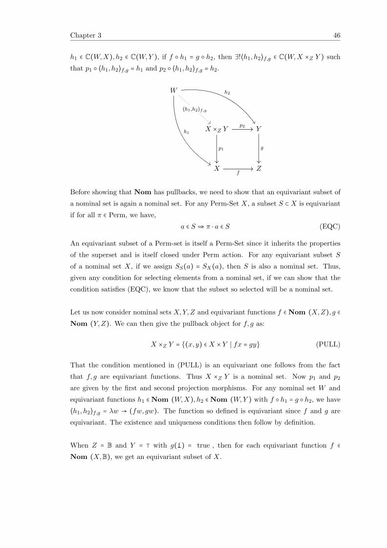
Chapter 3 46
h1 ∈ C(W,X), h2 ∈ C(W,Y ), if f ○ h1 = g ○ h2, then ∃!⟨h1, h2⟩f,g ∈ C(W,X ×Z Y ) such
that p1 ○ ⟨h1, h2⟩f,g = h1 and p2 ○ ⟨h1, h2⟩f,g = h2.
W
X ×Z Y Y
X Z
h2
h1
⟨h1,h2⟩f,g
p2
p1 g
f
Before showing that Nom has pullbacks, we need to show that an equivariant subset of
a nominal set is again a nominal set. For any Perm-Set X, a subset S ⊂X is equivariant
if for all π ∈ Perm, we have,
a ∈ S ⇒ π ⋅ a ∈ S (EQC)
An equivariant subset of a Perm-set is itself a Perm-Set since it inherits the properties
of the superset and is itself closed under Perm action. For any equivariant subset S
of a nominal set X, if we assign SS(a) = SX(a), then S is also a nominal set. Thus,
given any condition for selecting elements from a nominal set, if we can show that the
condition satisfies (EQC), we know that the subset so selected will be a nominal set.
Let us now consider nominal sets X,Y,Z and equivariant functions f ∈ Nom (X,Z), g ∈
Nom (Y,Z). We can then give the pullback object for f, g as:
X ×Z Y = {(x, y) ∈X × Y ∣ fx = gy} (PULL)
That the condition mentioned in (PULL) is an equivariant one follows from the fact
that f, g are equivariant functions. Thus X ×Z Y is a nominal set. Now p1 and p2
are given by the first and second projection morphisms. For any nominal set W and
equivariant functions h1 ∈ Nom (W,X), h2 ∈ Nom (W,Y ) with f ○ h1 = g ○ h2, we have
⟨h1, h2⟩f,g = λw → (fw, gw). The function so defined is equivariant since f and g are
equivariant. The existence and uniqueness conditions then follow by definition.
When Z = B and Y = ⊺ with g(1) = true , then for each equivariant function f ∈
Nom (X,B), we get an equivariant subset of X.
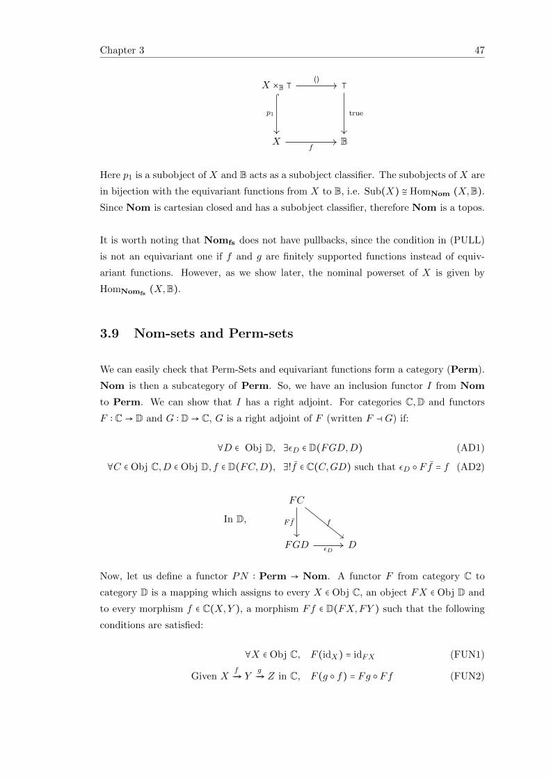
Chapter 3 47
X ×B ⊺ ⊺
X B
⟨⟩
p1 true
f
Here p1 is a subobject of X and B acts as a subobject classifier. The subobjects of X are
in bijection with the equivariant functions from X to B, i.e. Sub(X) ≅ HomNom (X,B).
Since Nom is cartesian closed and has a subobject classifier, therefore Nom is a topos.
It is worth noting that Nomfs does not have pullbacks, since the condition in (PULL)
is not an equivariant one if f and g are finitely supported functions instead of equiv-
ariant functions. However, as we show later, the nominal powerset of X is given by
HomNomfs(X,B).
3.9 Nom-sets and Perm-sets
We can easily check that Perm-Sets and equivariant functions form a category (Perm).
Nom is then a subcategory of Perm. So, we have an inclusion functor I from Nom
to Perm. We can show that I has a right adjoint. For categories C,D and functors
F ∶ C→ D and G ∶ D→ C, G is a right adjoint of F (written F ⊣ G) if:
∀D ∈ Obj D, ∃εD ∈ D(FGD,D) (AD1)
∀C ∈ Obj C,D ∈ Obj D, f ∈ D(FC,D), ∃!f ∈ C(C,GD) such that εD ○ F f = f (AD2)
In D,
FC
FGD D
F f f
εD
Now, let us define a functor PN ∶ Perm → Nom. A functor F from category C to
category D is a mapping which assigns to every X ∈ Obj C, an object FX ∈ Obj D and
to every morphism f ∈ C(X,Y ), a morphism Ff ∈ D(FX,FY ) such that the following
conditions are satisfied:
∀X ∈ Obj C, F (idX) = idFX (FUN1)
Given XfÐ→ Y
gÐ→ Z in C, F (g ○ f) = Fg ○ Ff (FUN2)
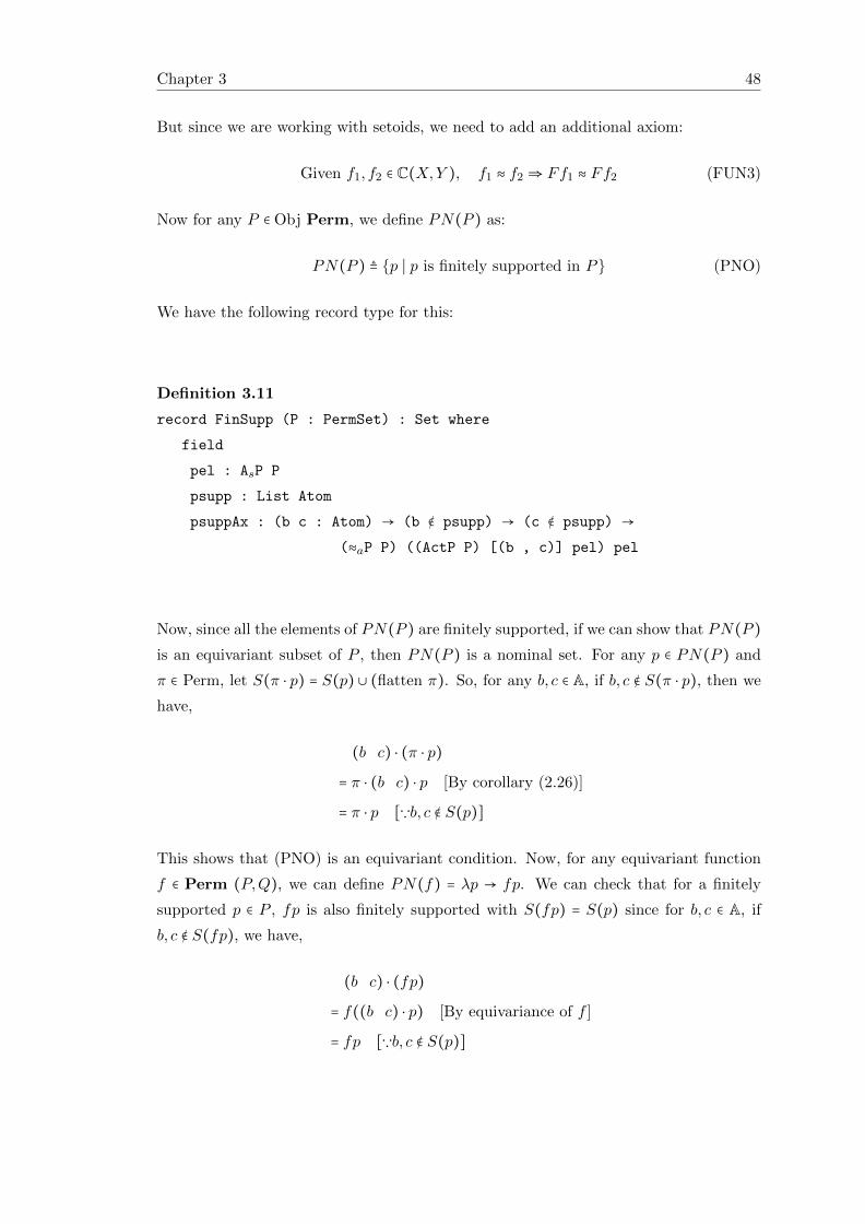
Chapter 3 48
But since we are working with setoids, we need to add an additional axiom:
Given f1, f2 ∈ C(X,Y ), f1 ≈ f2 ⇒ Ff1 ≈ Ff2 (FUN3)
Now for any P ∈ Obj Perm, we define PN(P ) as:
PN(P ) ≜ {p ∣ p is finitely supported in P} (PNO)
We have the following record type for this:
Definition 3.11
record FinSupp (P : PermSet) : Set where
field
pel : AsP P
psupp : List Atom
psuppAx : (b c : Atom) → (b ∉ psupp) → (c ∉ psupp) →
(≈aP P) ((ActP P) [(b , c)] pel) pel
Now, since all the elements of PN(P ) are finitely supported, if we can show that PN(P )
is an equivariant subset of P , then PN(P ) is a nominal set. For any p ∈ PN(P ) and
π ∈ Perm, let S(π ⋅ p) = S(p) ∪ (flatten π). So, for any b, c ∈ A, if b, c ∉ S(π ⋅ p), then we
have,
(b c) ⋅ (π ⋅ p)
= π ⋅ (b c) ⋅ p [By corollary (2.26)]
= π ⋅ p [∵b, c ∉ S(p)]
This shows that (PNO) is an equivariant condition. Now, for any equivariant function
f ∈ Perm (P,Q), we can define PN(f) = λp → fp. We can check that for a finitely
supported p ∈ P , fp is also finitely supported with S(fp) = S(p) since for b, c ∈ A, if
b, c ∉ S(fp), we have,
(b c) ⋅ (fp)
= f((b c) ⋅ p) [By equivariance of f ]
= fp [∵b, c ∉ S(p)]
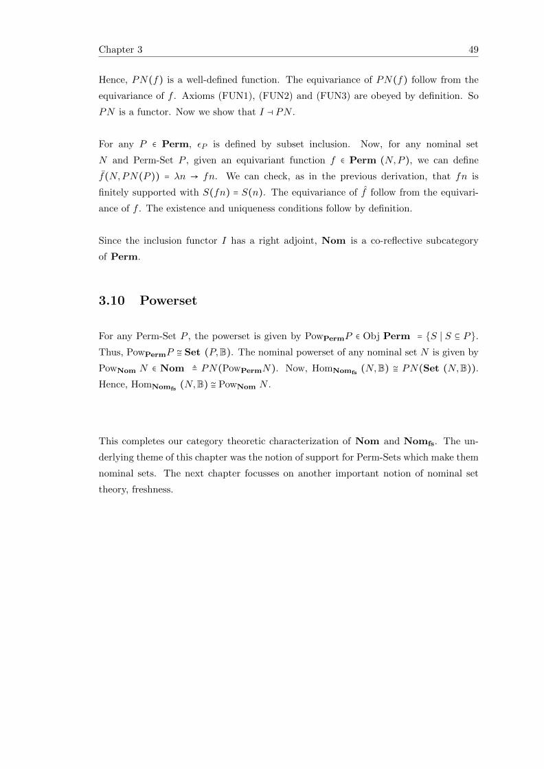
Chapter 3 49
Hence, PN(f) is a well-defined function. The equivariance of PN(f) follow from the
equivariance of f . Axioms (FUN1), (FUN2) and (FUN3) are obeyed by definition. So
PN is a functor. Now we show that I ⊣ PN .
For any P ∈ Perm, εP is defined by subset inclusion. Now, for any nominal set
N and Perm-Set P , given an equivariant function f ∈ Perm (N,P ), we can define
f(N,PN(P )) = λn → fn. We can check, as in the previous derivation, that fn is
finitely supported with S(fn) = S(n). The equivariance of f follow from the equivari-
ance of f . The existence and uniqueness conditions follow by definition.
Since the inclusion functor I has a right adjoint, Nom is a co-reflective subcategory
of Perm.
3.10 Powerset
For any Perm-Set P , the powerset is given by PowPermP ∈ Obj Perm = {S ∣ S ⊆ P}.
Thus, PowPermP ≅ Set (P,B). The nominal powerset of any nominal set N is given by
PowNom N ∈ Nom ≜ PN(PowPermN). Now, HomNomfs(N,B) ≅ PN(Set (N,B)).
Hence, HomNomfs(N,B) ≅ PowNom N .
This completes our category theoretic characterization of Nom and Nomfs. The un-
derlying theme of this chapter was the notion of support for Perm-Sets which make them
nominal sets. The next chapter focusses on another important notion of nominal set
theory, freshness.

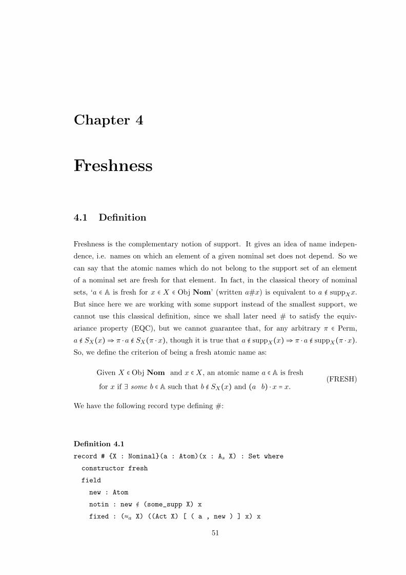
Chapter 4
Freshness
4.1 Definition
Freshness is the complementary notion of support. It gives an idea of name indepen-
dence, i.e. names on which an element of a given nominal set does not depend. So we
can say that the atomic names which do not belong to the support set of an element
of a nominal set are fresh for that element. In fact, in the classical theory of nominal
sets, ‘a ∈ A is fresh for x ∈ X ∈ Obj Nom’ (written a#x) is equivalent to a ∉ suppXx.
But since here we are working with some support instead of the smallest support, we
cannot use this classical definition, since we shall later need # to satisfy the equiv-
ariance property (EQC), but we cannot guarantee that, for any arbitrary π ∈ Perm,
a ∉ SX(x)⇒ π ⋅ a ∉ SX(π ⋅ x), though it is true that a ∉ suppX(x)⇒ π ⋅ a ∉ suppX(π ⋅ x).
So, we define the criterion of being a fresh atomic name as:
Given X ∈ Obj Nom and x ∈X, an atomic name a ∈ A is fresh
for x if ∃ some b ∈ A such that b ∉ SX(x) and (a b) ⋅ x = x.(FRESH)
We have the following record type defining #:
Definition 4.1
record # {X : Nominal}(a : Atom)(x : As X) : Set where
constructor fresh
field
new : Atom
notin : new ∉ (some_supp X) x
fixed : (≈a X) ((Act X) [ ( a , new ) ] x) x
51
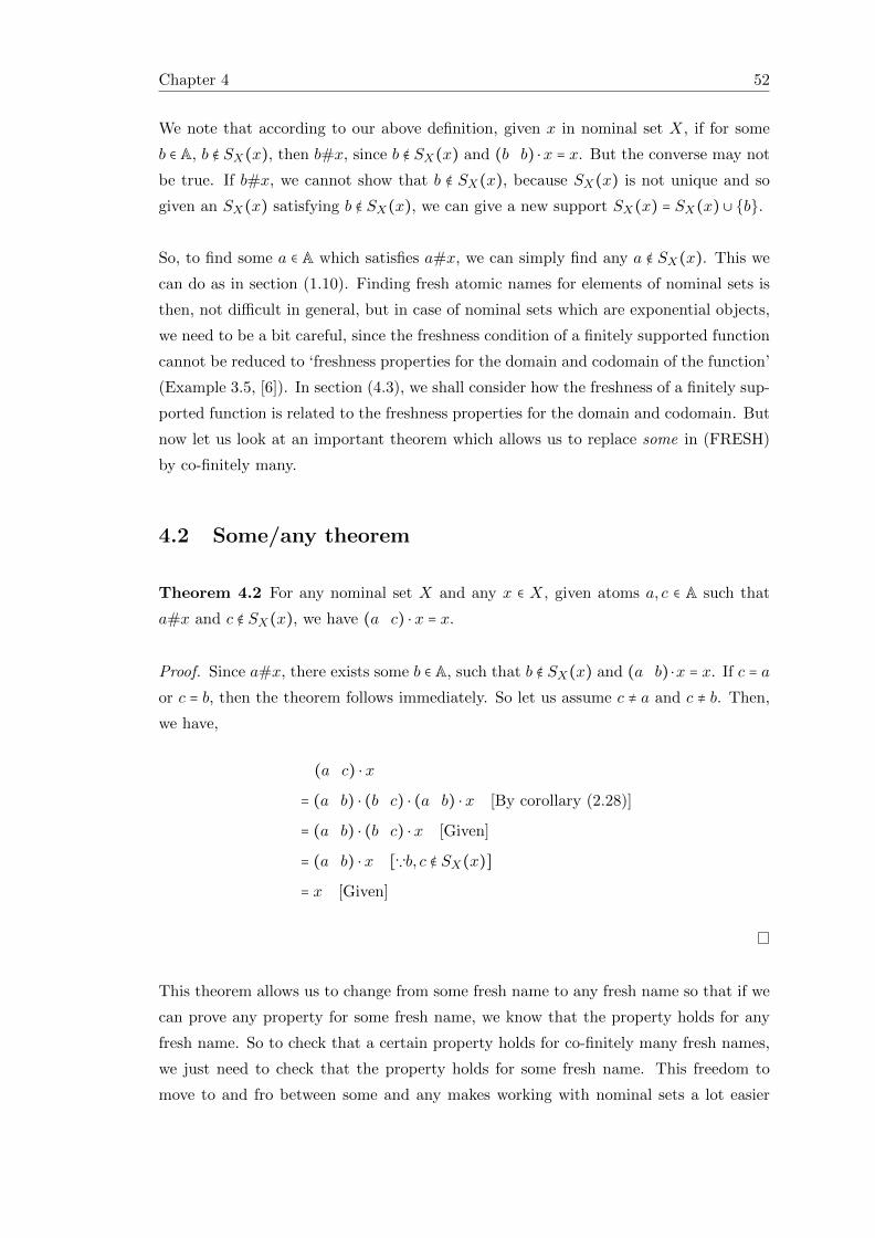
Chapter 4 52
We note that according to our above definition, given x in nominal set X, if for some
b ∈ A, b ∉ SX(x), then b#x, since b ∉ SX(x) and (b b) ⋅x = x. But the converse may not
be true. If b#x, we cannot show that b ∉ SX(x), because SX(x) is not unique and so
given an SX(x) satisfying b ∉ SX(x), we can give a new support SX(x) = SX(x) ∪ {b}.
So, to find some a ∈ A which satisfies a#x, we can simply find any a ∉ SX(x). This we
can do as in section (1.10). Finding fresh atomic names for elements of nominal sets is
then, not difficult in general, but in case of nominal sets which are exponential objects,
we need to be a bit careful, since the freshness condition of a finitely supported function
cannot be reduced to ‘freshness properties for the domain and codomain of the function’
(Example 3.5, [6]). In section (4.3), we shall consider how the freshness of a finitely sup-
ported function is related to the freshness properties for the domain and codomain. But
now let us look at an important theorem which allows us to replace some in (FRESH)
by co-finitely many.
4.2 Some/any theorem
Theorem 4.2 For any nominal set X and any x ∈ X, given atoms a, c ∈ A such that
a#x and c ∉ SX(x), we have (a c) ⋅ x = x.
Proof. Since a#x, there exists some b ∈ A, such that b ∉ SX(x) and (a b) ⋅x = x. If c = a
or c = b, then the theorem follows immediately. So let us assume c ≠ a and c ≠ b. Then,
we have,
(a c) ⋅ x
= (a b) ⋅ (b c) ⋅ (a b) ⋅ x [By corollary (2.28)]
= (a b) ⋅ (b c) ⋅ x [Given]
= (a b) ⋅ x [∵b, c ∉ SX(x)]
= x [Given]
This theorem allows us to change from some fresh name to any fresh name so that if we
can prove any property for some fresh name, we know that the property holds for any
fresh name. So to check that a certain property holds for co-finitely many fresh names,
we just need to check that the property holds for some fresh name. This freedom to
move to and fro between some and any makes working with nominal sets a lot easier
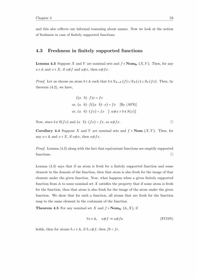
Chapter 4 53
and this also reflects our informal reasoning about names. Now we look at the notion
of freshness in case of finitely supported functions.
4.3 Freshness in finitely supported functions
Lemma 4.3 Suppose X and Y are nominal sets and f ∈ Nomfs (X,Y ). Then, for any
a ∈ A and x ∈X, if a#f and a#x, then a#fx.
Proof. Let us choose an atom b ∈ A such that b ∉ SX→Y (f)∪SX(x)∪SY (fx). Then, by
theorem (4.2), we have,
((a b) ⋅ f)x = fx
or, (a b) ⋅ f((a b) ⋅ x) = fx [By (AFS)]
or, (a b) ⋅ (fx) = fx [∵a#x ∧ b ∉ S(x)]
Now, since b ∉ S(fx) and (a b) ⋅ (fx) = fx, so a#fx.
Corollary 4.4 Suppose X and Y are nominal sets and f ∈ Nom (X,Y ). Then, for
any a ∈ A and x ∈X, if a#x, then a#fx.
Proof. Lemma (4.3) along with the fact that equivariant functions are emptily supported
functions.
Lemma (4.3) says that if an atom is fresh for a finitely supported function and some
element in the domain of the function, then that atom is also fresh for the image of that
element under the given function. Now, what happens when a given finitely supported
function from A to some nominal set X satisfies the property that if some atom is fresh
for the function, then that atom is also fresh for the image of the atom under the given
function. We show that for such a function, all atoms that are fresh for the function
map to the same element in the codomain of the function.
Theorem 4.5 For any nominal set X and f ∈ Nomfs (A,X), if
∀a ∈ A, a#f ⇒ a#fa (FCON)
holds, then for atoms b, c ∈ A, if b, c#f , then fb = fc.
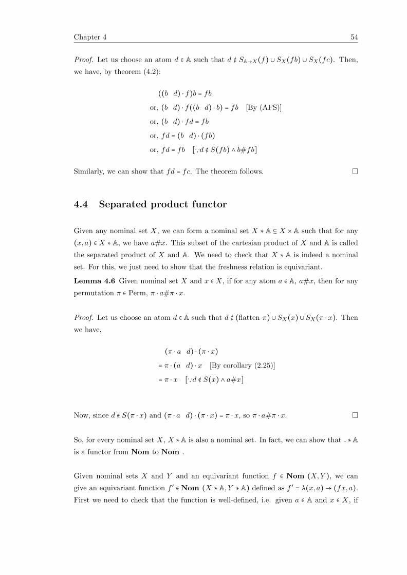
Chapter 4 54
Proof. Let us choose an atom d ∈ A such that d ∉ SA→X(f) ∪ SX(fb) ∪ SX(fc). Then,
we have, by theorem (4.2):
((b d) ⋅ f)b = fb
or, (b d) ⋅ f((b d) ⋅ b) = fb [By (AFS)]
or, (b d) ⋅ fd = fb
or, fd = (b d) ⋅ (fb)
or, fd = fb [∵d ∉ S(fb) ∧ b#fb]
Similarly, we can show that fd = fc. The theorem follows.
4.4 Separated product functor
Given any nominal set X, we can form a nominal set X ∗A ⊆ X ×A such that for any
(x, a) ∈ X ∗A, we have a#x. This subset of the cartesian product of X and A is called
the separated product of X and A. We need to check that X ∗ A is indeed a nominal
set. For this, we just need to show that the freshness relation is equivariant.
Lemma 4.6 Given nominal set X and x ∈X, if for any atom a ∈ A, a#x, then for any
permutation π ∈ Perm, π ⋅ a#π ⋅ x.
Proof. Let us choose an atom d ∈ A such that d ∉ (flatten π) ∪ SX(x) ∪ SX(π ⋅ x). Then
we have,
(π ⋅ a d) ⋅ (π ⋅ x)
= π ⋅ (a d) ⋅ x [By corollary (2.25)]
= π ⋅ x [∵d ∉ S(x) ∧ a#x]
Now, since d ∉ S(π ⋅ x) and (π ⋅ a d) ⋅ (π ⋅ x) = π ⋅ x, so π ⋅ a#π ⋅ x.
So, for every nominal set X, X ∗A is also a nominal set. In fact, we can show that ∗Ais a functor from Nom to Nom .
Given nominal sets X and Y and an equivariant function f ∈ Nom (X,Y ), we can
give an equivariant function f ′ ∈ Nom (X ∗A, Y ∗A) defined as f ′ = λ(x, a)→ (fx, a).
First we need to check that the function is well-defined, i.e. given a ∈ A and x ∈ X, if
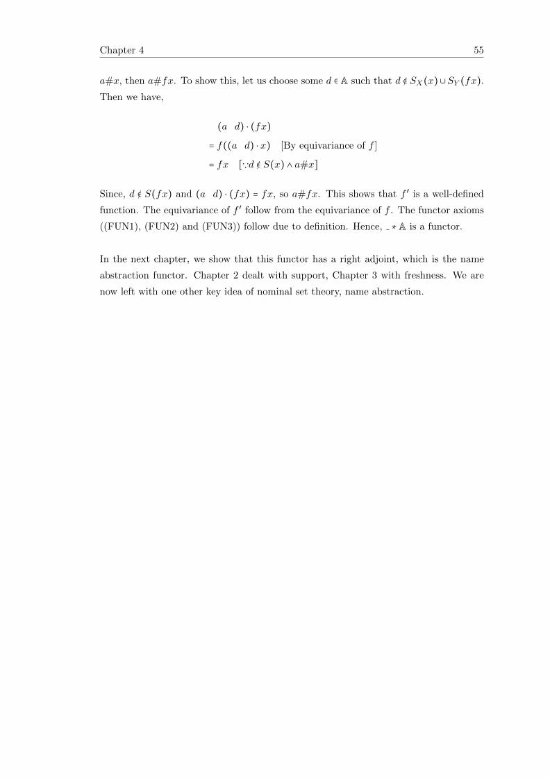
Chapter 4 55
a#x, then a#fx. To show this, let us choose some d ∈ A such that d ∉ SX(x)∪SY (fx).
Then we have,
(a d) ⋅ (fx)
= f((a d) ⋅ x) [By equivariance of f ]
= fx [∵d ∉ S(x) ∧ a#x]
Since, d ∉ S(fx) and (a d) ⋅ (fx) = fx, so a#fx. This shows that f ′ is a well-defined
function. The equivariance of f ′ follow from the equivariance of f . The functor axioms
((FUN1), (FUN2) and (FUN3)) follow due to definition. Hence, ∗A is a functor.
In the next chapter, we show that this functor has a right adjoint, which is the name
abstraction functor. Chapter 2 dealt with support, Chapter 3 with freshness. We are
now left with one other key idea of nominal set theory, name abstraction.

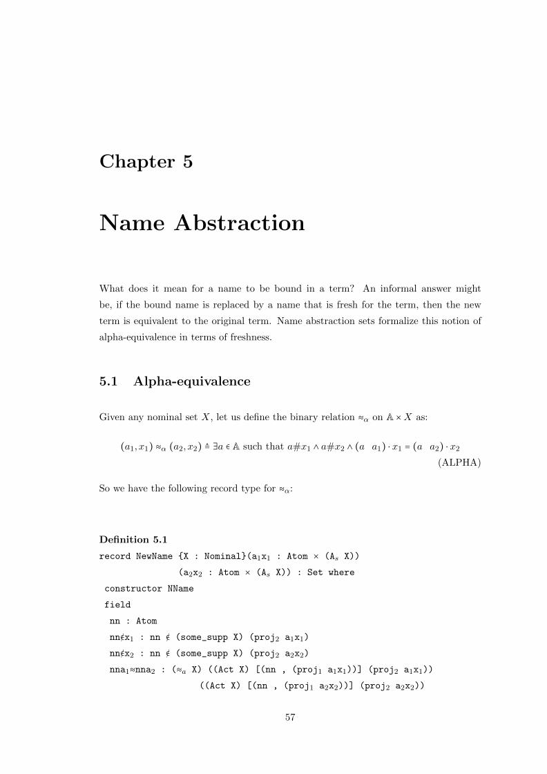
Chapter 5
Name Abstraction
What does it mean for a name to be bound in a term? An informal answer might
be, if the bound name is replaced by a name that is fresh for the term, then the new
term is equivalent to the original term. Name abstraction sets formalize this notion of
alpha-equivalence in terms of freshness.
5.1 Alpha-equivalence
Given any nominal set X, let us define the binary relation ≈α on A ×X as:
(a1, x1) ≈α (a2, x2) ≜ ∃a ∈ A such that a#x1 ∧ a#x2 ∧ (a a1) ⋅ x1 = (a a2) ⋅ x2
(ALPHA)
So we have the following record type for ≈α:
Definition 5.1
record NewName {X : Nominal}(a1x1 : Atom × (As X))
(a2x2 : Atom × (As X)) : Set where
constructor NName
field
nn : Atom
nn∉x1 : nn ∉ (some_supp X) (proj2 a1x1)
nn∉x2 : nn ∉ (some_supp X) (proj2 a2x2)
nna1≈nna2 : (≈a X) ((Act X) [(nn , (proj1 a1x1))] (proj2 a1x1))
((Act X) [(nn , (proj1 a2x2))] (proj2 a2x2))
57
Chapter 5 58
In line with some/any theorem (4.2), we have the following for (ALPHA):
Lemma 5.2
(a1, x1) ≈α (a2, x2)⇒ (∀c ∈ A, c#x1 ∧ c#x2 ⇒ (c a1) ⋅ x1 = (c a2) ⋅ x2) (ALPHA’)
Proof. Since (a1, x1) ≈α (a2, x2), by (ALPHA), there exists some b ∈ A such that:
b#x1 ∧ b#x2 ∧ (b a1) ⋅ x1 = (b a2) ⋅ x2 (ThC1)
Now we check the following cases:
� b = c
Theorem follows immediately.
� b = a1 ∧ c = a2 ∧ b ≠ a2 ∧ c ≠ a1
By (ThC1), x1 = (a1 a2) ⋅ x2 and hence (a2 a1) ⋅ x1 = x2.
� b = a2 ∧ c = a1 ∧ b ≠ a1 ∧ c ≠ a2
Similar to the previous case.
� b ≠ a1 ∧ c ≠ a1 ∧ b ≠ a2 ∧ c ≠ a2
We have,
(b a1) ⋅ x1 = (b a2) ⋅ x2
or, (c b) ⋅ (b a1) ⋅ x1 = (c b) ⋅ (b a2) ⋅ x2
or, (c b) ⋅ (b a1) ⋅ (c b) ⋅ x1 = (c b) ⋅ (b a2) ⋅ (c b) ⋅ x2 [∵b, c#x1 ∧ b, c#x2]
or, (c a1) ⋅ x1 = (c a2) ⋅ x2 [By corollary (2.28)]
The lemma follows.
Now, we prove that ≈α is an equivalence relation. Reflexivity and symmetricity are easy
to check. We prove the transitivity of ≈α.
Lemma 5.3 ≈α is transitive.
Proof. Let (a1, x1) ≈α (a2, x2) and (a2, x2) ≈α (a3, x3). Let us choose c ∈ A such that
c ∉ SX(x1) ∪ SX(x2) ∪ SX(x3). Therefore by lemma (5.2), (c a1) ⋅ x1 = (c a2) ⋅ x2
and (c a2) ⋅ x2 = (c a3) ⋅ x3. So c#x1 and c#x3 and (c a1) ⋅ x1 = (c a3) ⋅ x3. Hence
(a1, x1) ≈α (a3, x3).
We now prove a few lemmas on ≈α.
Chapter 5 59
Lemma 5.4 Given (a1, x1) ≈α (a2, x2), if a1 = a2 then x1 = x2.
Proof. Since (a1, x1) ≈α (a2, x2), so for some b ∈ A, we have (b a1) ⋅ x1 = (b a2) ⋅ x2.
But since a1 = a2, so x1 = x2.
Lemma 5.5 Given (a1, x1) ≈α (a2, x2), if a1#x1 and a2#x2, then x1 = x2.
Proof. Since (a1, x1) ≈α (a2, x2), so for some b ∈ A, we have b#x1 and b#x2 and (b a1) ⋅
x1 = (b a2) ⋅ x2. Now since b, a1#x1 and b, a2#x2, therefore x1 = x2.
Lemma 5.6 Given any nominal set X and x ∈ X, for atoms a, a′ ∈ A, if a′#x, then
(a, x) ≈α (a′, (a′ a) ⋅ x).
Proof. Let us choose some b ∈ A such that b ∉ SX(x) ∪ SX((a′ a) ⋅ x). Then we have,
(b a′) ⋅ ((a′ a) ⋅ x)
= (b a′) ⋅ (a′ a) ⋅ (b a′) ⋅ x [∵b ∉ S(x) ∧ a′#x]
= (b a) ⋅ x [By corollary (2.28)]
Now, b#x and b#(a′ a) ⋅x and (b a) ⋅x = (b a′) ⋅ ((a′ a) ⋅x). The lemma follows.
Given any term, we can change to any other member of the alpha-equivalence class of
the term using the above lemma. Now we can define name abstraction sets.
5.2 Name abstraction sets
Given a nominal set X, the set A × X quotiented by ≈α is called the set of name
abstractions of elements of X. It is denoted by [A]X. We now prove that [A]X is
indeed a nominal set. Since we are working with setoids, we declare the underlying set
of [A]X to be A×X and the underlying relation to be ≈α. The associativity and identity
group action axioms ((GA1) and (GA2)) follow from their corresponding counterparts
for A and X. Now we need to verify axiom (GA3), that equivalent permutations act on
equivalent elements of A ×X to give equivalent elements.
Lemma 5.7 Given π1, π2 ∈ Perm and (a1, x1), (a2, x2) ∈ A×X, if π1 ≈ π2 and (a1, x1) ≈α
(a2, x2), then (π1 ⋅ a1, π1 ⋅ x1) ≈α (π2 ⋅ a2, π2 ⋅ x2).
Proof. Let us choose b ∈ A such that b ∉ (flatten π1) ∪ (flatten π2) ∪ SX(x1) ∪ SX(x2) ∪
SX(π1 ⋅ x1) ∪ SX(π2 ⋅ x2). So, by lemma (5.2),
Chapter 5 60
(b a1) ⋅ x1 = (b a2) ⋅ x2
Now, we have,
(b π1 ⋅ a1) ⋅ (π1 ⋅ x1)
= π1 ⋅ (b a1) ⋅ x1 [By corollary (2.25)]
= π1 ⋅ (b a2) ⋅ x2
= π2 ⋅ (b a2) ⋅ x2 [∵π1 ≈ π2]
= (b π2 ⋅ a2) ⋅ (π2 ⋅ x2) [By corollary (2.25)]
This along with the fact that b#π1 ⋅ x1 and b#π2 ⋅ x2 shows that (π1 ⋅ a1, π1 ⋅ x1) ≈α
(π2 ⋅ a2, π2 ⋅ x2).
Once (GA1), (GA2) and (GA3) are satisfied, we know that [A]X is a PermSet. Now
we give the support for any (a, x) ∈ [A]X as S[A]X(a, x) = SX(x). Next we show that
this indeed is a support.
Lemma 5.8 Given a nominal set X and x ∈X, for atoms a, b, c ∈ A, if b, c ∉ S[A]X(a, x),
then (b c) ⋅ (a, x) ≈α (a, x).
Proof. If b = a or c = a, then a#x and (b c) ⋅ a#x. The lemma then follows by lemma
(5.5). So, let us assume that b ≠ a and c ≠ a. Then, since b, c ∉ SX(x), so (b c) ⋅ (a, x) =
((b c) ⋅ a, (b c) ⋅ x) = (a, x). The lemma follows.
This shows that [A]X is a nominal set. In fact we can define a functor [A] ∶ Nom →
Nom , the name abstraction functor.
5.3 Name abstraction functor
Given nominal sets X and Y and an equivariant function f ∈ Nom (X,Y ), we have
f ′ ∈ Nom ([A]X, [A]Y ) defined as f ′ = λ(a, x) → (a, fx). First we need to show that
this respects ≈α (EqP2).
Lemma 5.9 Given f ∈ Nom (X,Y ) and (a1, x1) ≈α (a2, x2) ∈ [A]X, (a1, fx1) ≈α
(a2, fx2).
Proof. Let us choose b ∉ SX(x1)∪SX(x2)∪SY (fx1)∪SY (fx2). Then, by lemma (5.2),
(b a1) ⋅ x1 = (b a2) ⋅ x2
Chapter 5 61
Now, we have,
(b a1) ⋅ (fx1)
= f((b a1) ⋅ x1) [By equivariance of f ]
= f((b a2) ⋅ x2)
= (b a2) ⋅ (fx2) [By equivariance of f ]
This along with the fact that b#fx1 and b#fx2 shows that (a1, fx1) ≈α (a2, fx2).
Once we know that f ′ respects ≈α, we just need to check that it’s an equivariant function.
But this follows from the equivariance of f . This defines the functor [A] action on
morphisms. The functor axioms ((FUN1), (FUN2) and (FUN3)) follow by definition.
Hence [A] is a functor.
5.4 Properties of name abstraction functor
The name abstraction functor is very well-behaved, it preserves limits and colimits in
Nom. Below we check that [A] preserves products and coproducts.
Lemma 5.10 For nominal sets X1 and X2, [A](X1 ×X2) ≅ ([A]X1) × ([A]X2).
Proof. We need to give equivariant functions f and g respectively from [A](X1 ×X2) to
([A]X1) × ([A]X2) and vice-versa such that g ○ f and f ○ g are identity morphisms on
[A](X1 ×X2) and ([A]X1) × ([A]X2) respectively.
� f ∶ [A](X1 ×X2)→ ([A]X1) × ([A]X2)
We define f as f = λ(a, (x1, x2)) → ((a, x1), (a, x2)). We need to check that this
definition respects ≈α (EqP2). For this, let us consider (a, (x1, x2)), (a′, (x′1, x
′2)) ∈
[A](X1 ×X2) such that (a, (x1, x2)) ≈α (a′, (x′1, x′2)). Now we need to show that
((a, x1), (a, x2)) ≈α ((a′, x′1), (a′, x′2)).
Let us choose b ∈ A such that b ∉ SX1(x1) ∪ SX2(x2) ∪ SX1(x′1) ∪ SX2(x
′2). Then,
we have,
(b a) ⋅ (x1, x2) = (b a′) ⋅ (x′1, x′2)
or, (b a) ⋅ x1 = (b a′) ⋅ x′1 ∧ (b a) ⋅ x2 = (b a′) ⋅ x′2
or, (a, x1) ≈α (a′, x′1) ∧ (a, x2) ≈α (a′, x′2)
or, ((a, x1), (a, x2)) ≈α ((a′, x′1), (a′, x′2))
Chapter 5 62
Once we have shown that f respects ≈α, we need to check it is an equivariant
function. But that follows from the definition of f .
� g ∶ ([A]X1) × ([A]X2)→ [A](X1 ×X2)
Given ((a1, x1), (a2, x2)) ∈ ([A]X1)×([A]X2), we define g((a1, x1), (a2, x2)) in the
following way:
Let us choose some b ∈ A such that b ∉ {a1} ∪ {a2} ∪ SX1(x1) ∪ SX2(x2). Then
g((a1, x1), (a2, x2)) = (b, ((b a1) ⋅ x1, (b a2) ⋅ x2)).
We need to check that this definition of g respects ≈α (EqP2). For this, let
us consider ((a1, x1), (a2, x2)), ((a′1, x
′1), (a
′2, x
′2)) ∈ ([A]X1) × ([A]X2) such that
((a1, x1), (a2, x2)) ≈α ((a′1, x′1), (a
′2, x
′2)). We need to show that,
(b, ((b a1) ⋅ x1, (b a2) ⋅ x2)) ≈α (b′, ((b′ a′1) ⋅ x′1, (b
′ a′2) ⋅ x′2))
for some b ∉ {a1} ∪ {a2} ∪ SX1(x1) ∪ SX2(x2) and b′ ∉ {a′1} ∪ {a′2} ∪ SX1(x′1) ∪
SX2(x′2). For this, let us choose c ∈ A such that c ∉ {a1, a2, a
′1, a
′2} ∪ SX1(x1) ∪
SX2(x2)∪SX1(x′1)∪SX2(x
′2)∪SX1((b a1) ⋅ x1)∪SX2((b a2) ⋅ x2)∪SX1((b
′ a′1) ⋅
x′1) ∪ SX2((b′ a′2) ⋅ x
′2). Then we have,
(c b) ⋅ ((b a1) ⋅ x1)
= (c b) ⋅ (b a1) ⋅ (c b) ⋅ x1 [∵c, b ∉ S(x1)]
= (c a1) ⋅ x1 [By corollary (2.28)]
= (c a′1) ⋅ x′1 [∵(a1, x1) ≈α (a′1, x
′1)]
= (c b′) ⋅ (b′ a′1) ⋅ (c b′) ⋅ x′1 [By corollary (2.28)]
= (c b′) ⋅ ((b′ a′1) ⋅ x′1) [∵c, b′ ∉ S(x′1)]
Similarly, we can show that (c b) ⋅ ((b a2) ⋅ x2) = (c b′) ⋅ ((b′ a′2) ⋅ x′2). So,
(c b) ⋅ ((b a1) ⋅ x1, (b a2) ⋅ x2) = (c b′) ⋅ ((b′ a′1) ⋅ x′1, (b
′ a′2) ⋅ x′2)). Hence, g
respects ≈α. Now, we check that g is an equivariant function. For this, let us
suppose ((a1, x1), (a2, x2)) ∈ ([A]X1) × ([A]X2) and π ∈ Perm. Then, we need to
show that,
(π ⋅ b, (π ⋅ (b a1) ⋅x1, π ⋅ (b a2) ⋅x2)) ≈α (bπ, ((bπ π ⋅ a1) ⋅π ⋅x1, (bπ π ⋅ a2) ⋅π ⋅x2))
for some b ∉ {a1} ∪ {a2} ∪ SX1(x1) ∪ SX2(x2) and bπ ∉ {π ⋅ a1} ∪ {π ⋅ a2} ∪ SX1(π ⋅
x1) ∪ SX2(π ⋅ x2). To this end, let us choose c ∈ A such that c ∉ {a1, a2, π ⋅ a1, π ⋅
a2} ∪ (flatten π) ∪ SX1(x1) ∪ SX2(x2) ∪ SX1(π ⋅ x1) ∪ SX2(π ⋅ x2) ∪ SX1(π ⋅ (b a1) ⋅
Chapter 5 63
x1)∪SX2(π ⋅ (b a2) ⋅x2)∪SX1((bπ π ⋅ a1) ⋅π ⋅x1)∪SX2((bπ π ⋅ a2) ⋅π ⋅x2). Then,
we have,
(c π ⋅ b) ⋅ π ⋅ (b a1) ⋅ x1
= π ⋅ (c b) ⋅ (b a1) ⋅ x1 [By corollary(2.25)]
= π ⋅ (c b) ⋅ (b a1) ⋅ (c b) ⋅ x1 [∵c, b ∉ S(x1)]
= π ⋅ (c a1) ⋅ x1 [By corollary (2.28)]
= (c π ⋅ a1) ⋅ πx1 [By corollary (2.25)]
= (c bπ) ⋅ (bπ π ⋅ a1) ⋅ (c bπ) ⋅ π ⋅ x1 [By corollary (2.28)]
= (c bπ) ⋅ (bπ π ⋅ a1) ⋅ π ⋅ x1 [∵c, bπ ∉ S(π ⋅ x1)]
Similarly, we can show that (c π ⋅b)⋅π ⋅(b a2)⋅x2 = (c bπ)⋅(bπ π ⋅a2)⋅π ⋅x2. Hence,
(c π ⋅b) ⋅(π ⋅(b a1) ⋅x1, π ⋅(b a2) ⋅x2) = (c bπ) ⋅((bπ π ⋅a1) ⋅π ⋅x1, (bπ π ⋅a2) ⋅π ⋅x2).
This shows that g is an equivariant function.
� g ○ f = id
Suppose (a, (x1, x2)) ∈ [A](X1 ×X2). We have (g ○ f)(a, (x1, x2)) = (b, ((b a1) ⋅
x1, (b a2) ⋅ x2)) for some b ∈ A such that b ∉ {a} ∪ SX1(x1) ∪ SX2(x2). By lemma
(5.6), (a, (x1, x2)) ≈α (b, ((b a1) ⋅ x1, (b a2) ⋅ x2)).
� f ○ g = id
Suppose ((a1, x1), (a2, x2)) ∈ ([A]X1)×([A]X2). We have (f○g)((a1, x1), (a2, x2)) =
((b, (b a1) ⋅x1), (b, (b a2) ⋅x2)) for some b ∈ A such that b ∉ {a1}∪{a2}∪SX1(x1)∪
SX2(x2). By lemma (5.6), ((a1, x1), (a2, x2)) ≈α ((b, (b a1) ⋅ x1), (b, (b a2) ⋅ x2)).
The lemma follows.
Lemma 5.11 For nominal sets X1 and X2, [A](X1 +X2) ≅ ([A]X1) + ([A]X2).
Proof. We can give equivariant functions f and g respectively from [A](X1 + X2) to
([A]X1) + ([A]X2) and vice-versa as:
f(a,w) = match w with
∣ inl x1 → inl (a, x1)
∣ inr x2 → inr (a, x2)
gv = match v with
∣ inl (a, x1)→ (a, inl x1)
∣ inr (a, x2)→ (a, inr x2)
Chapter 5 64
We can easily check that both f and g satisfy axioms (EqP1) and (EqP2) and that g○f =
id and f ○ g = id.
The separated product functor encapsulates the notion of freshness whereas the name
abstraction functor the notion of alpha-equivalence. Applying these functors in succes-
sion to any nominal set gives us the following lemma.
Lemma 5.12 For any nominal set X, ([A]X) ∗A ≅ A ×X.
Proof. We can give equivariant functions f and g from ([A]X)∗A to A×X and vice-versa
respectively as:
f((a, x), a′) = (a′, (a′ a) ⋅ x)
g(a, x) = ((a, x), a)
We need to check that f satisfies axiom (EqP2), i.e. given ((a1, x1), a′), ((a2, x2), a
′) ∈
([A]X) ∗A, if (a1, x1) ≈α (a2, x2), then (a′ a1) ⋅ x1 = (a′ a2) ⋅ x2. But this is true, by
lemma (5.2), since a′#x1, x2. We now check that f satisfies the equivariance property
(EqP1). For this, let ((a, x), a′) ∈ ([A]X) ∗ A and π ∈ Perm. We need to show that
π ⋅ ((a′ a) ⋅x) = (π ⋅ a′ π ⋅ a) ⋅ (π ⋅x). But this follows from lemma (2.24). Hence f is an
equivariant function.
Now, we need to check that g is a well-defined function, i.e. a#(a, x) ∈ [A]X. But
this is true since for any b ∈ A, if b ∉ SX(x), then we have,
(b a) ⋅ (a, x)
≈α (b, (b a) ⋅ x)
≈α (a, x) [By lemma (5.6), ∵b#x]
Once we have shown that g is well-defined, we need to verify axioms (EqP1) and (EqP2).
But these follow easily from definition. Hence g is an equivariant function.
Now we show that g ○ f = id. Let ((a, x), a′) ∈ ([A]X) ∗A. Then, we have,
(g ○ f)((a, x), a′)
= g(a′, (a′ a) ⋅ x)
= ((a′, (a′ a) ⋅ x), a′)
Chapter 5 65
But by lemma (5.6), (a′, (a′ a) ⋅ x) ≈α (a, x) for a′#x. Hence g ○ f = id. Next we show
that f ○ g = id. Let (a, x) ∈ A ×X. Then, we have,
(f ○ g)(a, x)
= f((a, x), a)
= (a, (a a) ⋅ x)
= (a, x)
The lemma follows.
Now we show that the name abstraction functor has a left adjoint, the separated product
functor.
Theorem 5.13 ∗A ⊣ [A]
Proof. First we give the counit of the adjunction. For any nominal set X, let εX ∈
Nom (([A]X)∗A,X) defined as εX = λ((a, x), a′)→ (a′ a) ⋅x. First, we check that εX
satisfies axiom (EqP2). Let ((a1, x1), a′), ((a2, x2), a
′) ∈ ([A])X∗A such that (a1, x1) ≈α
(a2, x2). We need to show that (a′ a1) ⋅x1 = (a′ a2) ⋅x2. But this is true by (5.2), since
a′#x1, x2. Now we check for equivariance (EqP1). Let ((a, x), a′) ∈ ([A])X ∗A and π ∈
Perm. Then, we have,
π ⋅ εX((a, x), a′)
= π ⋅ (a′ a) ⋅ x
= (π ⋅ a′ π ⋅ a) ⋅ π ⋅ x [By lemma (2.24)]
= εX(π ⋅ ((a, x), a′))
Once we have shown that εX is an equivariant function, we need to show that it has the
required universal property. Let X,Y are nominal sets and f ∈ Nom (Y ∗ A,X). We
define f ∈ Nom (Y, [A]X) in the following way.
For any y ∈ Y , let us choose b ∈ A such that b#y. Then (y, b) ∈ Y ∗A.
So, f(y) = f(y, b) is well-defined.
But we need to check that f ∈ Nom (Y, [A]X). First we verify axiom (EqP2), i.e. given
y1, y2 ∈ Y such that y1 ≈ y2 (where ≈ is the underlying relation on setoid Y ), we show
that (b1, f(y1, b1)) ≈α (b2, f(y2, b2)), where b1#y1 and b2#y2. Let us choose c ∈ A such
Chapter 5 66
that c ∉ SY (y1) ∪ SY (y2) ∪ SX(f(y1, b1)) ∪ SX(f(y2, b2)). Then, we have,
(c b1) ⋅ f(y1, b1)
= f((c b1) ⋅ y1, (c b1) ⋅ b1) [By equivariance of f ]
= f(y1, c) [∵b1#y1 ∧ c ∉ S(y1)]
= f(y2, c) [∵f respects ≈]
= f((c b2) ⋅ y2, (c b2) ⋅ b2) [∵b2#y2 ∧ c ∉ S(y2)]
= (c b2) ⋅ f(y2, b2) [By equivariance of f ]
Hence, (b1, f(y1, b1)) ≈α (b2, f(y2, b2)). We now check that f satisfies equivariance
property (EqP1). Let y ∈ Y and let f(y) = (b, f(y, b)) for some b ∈ A such that b#y.
Also, let π ∈ Perm. Now let f(π ⋅y) = (bπ, f(π ⋅y, bπ)) for some bπ ∈ A such that bπ#π ⋅y.
We need to show that (π ⋅ b, π ⋅ f(y, b)) ≈α (bπ, f(π ⋅ y, bπ)). For this, let us choose c ∈ Asuch that c ∉ (flatten π) ∪ SY (y) ∪ SY (π ⋅ y) ∪ SX(f(y, b)) ∪ SX(f(π ⋅ y, bπ)). Then, we
have,
(c π ⋅ b) ⋅ (π ⋅ f(y, b))
= π ⋅ (c b) ⋅ f(y, b) [By lemma (2.24)]
= π ⋅ f((c b) ⋅ y, (c b) ⋅ b) [By equivariance of f ]
= π ⋅ f(y, c) [∵b#y ∧ c ∉ S(y)]
= f(π ⋅ y, π ⋅ c) [By equivariance of f ]
= f(π ⋅ y, c) [By lemma (2.23)]
= f((c bπ) ⋅ π ⋅ y, (c bπ) ⋅ bπ) [∵bπ#π ⋅ y ∧ c ∉ S(π ⋅ y)]
= (c bπ) ⋅ f(π ⋅ y, bπ) [By equivariance of f ]
This shows that (π ⋅ b, π ⋅ f(y, b)) ≈α (bπ, f(π ⋅ y, bπ)). Hence f ∈ Nom (Y, [A]X).
Now we check the existence condition. Let (y, a) ∈ Y ∗ A. Then, (f ∗ idA)(y, a) =
((b, f(y, b)), a) for some b#y. This gives,
εX((b, f(y, b)), a)
= (a b) ⋅ f(y, b) [By definition]
= f((a b) ⋅ y, (a b) ⋅ b) [By equivariance of f ]
= f(y, a) [∵a#y ∧ b#y]
This shows that the triangle below commutes.
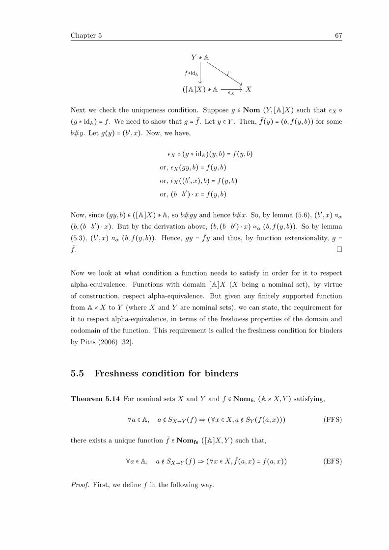
Chapter 5 67
Y ∗A
([A]X) ∗A X
f∗idA f
εX
Next we check the uniqueness condition. Suppose g ∈ Nom (Y, [A]X) such that εX ○
(g ∗ idA) = f . We need to show that g = f . Let y ∈ Y . Then, f(y) = (b, f(y, b)) for some
b#y. Let g(y) = (b′, x). Now, we have,
εX ○ (g ∗ idA)(y, b) = f(y, b)
or, εX(gy, b) = f(y, b)
or, εX((b′, x), b) = f(y, b)
or, (b b′) ⋅ x = f(y, b)
Now, since (gy, b) ∈ ([A]X) ∗A, so b#gy and hence b#x. So, by lemma (5.6), (b′, x) ≈α(b, (b b′) ⋅ x). But by the derivation above, (b, (b b′) ⋅ x) ≈α (b, f(y, b)). So by lemma
(5.3), (b′, x) ≈α (b, f(y, b)). Hence, gy = fy and thus, by function extensionality, g =
f .
Now we look at what condition a function needs to satisfy in order for it to respect
alpha-equivalence. Functions with domain [A]X (X being a nominal set), by virtue
of construction, respect alpha-equivalence. But given any finitely supported function
from A ×X to Y (where X and Y are nominal sets), we can state, the requirement for
it to respect alpha-equivalence, in terms of the freshness properties of the domain and
codomain of the function. This requirement is called the freshness condition for binders
by Pitts (2006) [32].
5.5 Freshness condition for binders
Theorem 5.14 For nominal sets X and Y and f ∈ Nomfs (A ×X,Y ) satisfying,
∀a ∈ A, a ∉ SX→Y (f)⇒ (∀x ∈X,a ∉ SY (f(a, x))) (FFS)
there exists a unique function f ∈ Nomfs ([A]X,Y ) such that,
∀a ∈ A, a ∉ SX→Y (f)⇒ (∀x ∈X, f(a, x) = f(a, x)) (EFS)
Proof. First, we define f in the following way.
Chapter 5 68
Let (a, x) ∈ [A]X. Let us choose some b ∈ A such that b ∉ {a} ∪ SX→Y (f) ∪ SX(x).
Then f(a, x) = f(b, (b a) ⋅ x).
We now prove that f is a finitely supported function with S[A]X→Y (f) = SA×X→Y (f).
But before that, we need to prove a lemma.
Lemma 5.15 Given a1, a2 ∈ A and x1, x2 ∈ X such that a1, a2 ∉ SA×X→Y (f) and
(a1, x1) ≈α (a2, x2) holds, then f(a1, x1) = f(a2, x2).
Proof. Let us choose a3 ∈ A such that a3 ∉ SX(x1)∪SX(x2)∪SY (f(a1, x1))∪SY (f(a2, x2))∪
SA×X→Y (f). Then we have,
f(a1, x1)
= (a3 a1) ⋅ (f(a1, x1)) [∵a3 ∉ S(f(a1, x1)) ∧ a1 ∉ S(f(a1, x1))]
= f((a3 a1) ⋅ (a1, x1)) [∵a3, a1 ∉ S(f)]
= f(a3, (a3 a1) ⋅ x1)
Similarly, we can show that f(a2, x2) = f(a3, (a3 a2)⋅x2). But since (a1, x1) ≈α (a2, x2),
so (a3 a1) ⋅ x1 = (a3 a2) ⋅ x2. The lemma follows.
Now we shall verify axiom (FS1). Let c, d ∈ A such that c, d ∉ S(f). Let (a, x) ∈
[A] × X. Now f(a, x) = f(b, (b a) ⋅ x) = y1 (say) for some b ∉ {a} ∪ S(f) ∪ S(x).
And f((c d) ⋅ a, (c d) ⋅ x) = f(b′, (b′ (c d) ⋅ a) ⋅ (c d) ⋅ x) = y2 (say) for some b′ ∉
{(c d) ⋅ a} ∪ S(f) ∪ S((c d) ⋅ x). We need to show that (c d) ⋅ y2 = y1. For this, let us
choose m ∈ A such that m ∉ {c, d, (c d) ⋅ a} ∪ S(f) ∪ S(y2) ∪ S(x) ∪ S((c d) ⋅ x). Then,
we have,
(c d) ⋅ y2
= (c d) ⋅ (m b′) ⋅ y2 [∵m,b′ ∉ S(y2)]
= (c d) ⋅ f(m b′) ⋅ (b′, (b′ (c d) ⋅ a) ⋅ (c d) ⋅ x) [∵m,b′ ∉ f]
= (c d) ⋅ f(m, (m b′) ⋅ (b′ (c d) ⋅ a) ⋅ (c d) ⋅ x)
= (c d) ⋅ f(m, (m b′) ⋅ (b′ (c d) ⋅ a) ⋅ (m b′) ⋅ (c d) ⋅ x)
[∵m,b′ ∉ S((c d) ⋅ x)]
= (c d) ⋅ f(m, (m (c d) ⋅ a) ⋅ (c d) ⋅ x) [By lemma (2.28)]
= (c d) ⋅ f((c d) ⋅m, (c d) ⋅ (m a) ⋅ x) [By corollary (2.25)]
= (c d) ⋅ f(c d) ⋅ (m, (m a) ⋅ x)
= f(m, (m a) ⋅ x) [∵c, d ∉ S(f)]
= f(b, (b a) ⋅ x) [By lemma (5.15)]
Chapter 5 69
To show that f is a finitely supported function, we need to verify axiom (FS2) as well.
But this follows from lemma (5.15). Now we shall prove the existence and uniqueness
conditions. The existence condition follows from lemma (5.15). To prove the uniqueness
condition, let us assume g ∈ Nomfs ([A]X,Y ) satisfies EFS. We need to show that
g = f . Let (a, x) ∈ [A]X. Let f(a, x) = f(b, (b a) ⋅ x) for some b ∈ A such that
b ∉ {a} ∪ S(f) ∪ S(x). Now, we have,
g(a, x)
= g(b, (b a) ⋅ x) [∵g respects ≈α]
= f(b, (b a) ⋅ x) [∵b ∉ S(f)]
= f(a, x)
The lemma follows.
Equivariant functions are emptily supported functions. So for equivariant functions, we
have the following corollary of the above theorem.
Corollary 5.16 For nominal sets X,Y,Z and f ∈ Nom (X ×A × Y,Z) satisfying,
∀x ∈X,a ∈ A, a ∉ SX(x)⇒ ((∀y ∈ Y ), a ∉ SZ(f(x, a, y))) (FEQ)
there exists a unique f ∈ Nom (X × [A]Y,Z) such that,
∀x ∈X,a ∈ A, a ∉ SX(x)⇒ ((∀y ∈ Y ), f(x, a, y) = f(x, a, y)) (EEQ)
Proof. First, we define f in the following way.
Let (x, a, y) ∈X × [A]Y . Let us choose b ∈ A such that b ∉ {a} ∪ SX(x) ∪ SY (y). Then
f(x, a, y) = f(x, b, (b a) ⋅ y).
In order to show that f is an equivariant function, we need to prove a lemma.
Lemma 5.17 Given x ∈ X and (a1, y1), (a2, y2) ∈ [A]Y such that a1, a2 ∉ SX(x) and
(a1, y1) ≈α (a2, y2), we have f(x, a1, y1) = f(x, a2, y2).
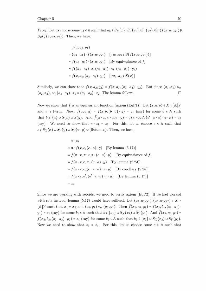
Chapter 5 70
Proof. Let us choose some a3 ∈ A such that a3 ∉ SX(x)∪SY (y1)∪SY (y2)∪SZ(f(x, a1, y1))∪
SZ(f(x, a2, y2)). Then, we have,
f(x, a1, y1)
= (a3 a1) ⋅ f(x, a1, y1) [∵a1, a3 ∉ S(f(x, a1, y1))]
= f(a3 a1) ⋅ (x, a1, y1) [By equivariance of f ]
= f((a3 a1) ⋅ x, (a3 a1) ⋅ a1, (a3 a1) ⋅ y1)
= f(x, a3, (a3 a1) ⋅ y1) [∵a1, a3 ∉ S(x)]
Similarly, we can show that f(x, a2, y2) = f(x, a3, (a3 a2) ⋅ y2). But since (a1, x1) ≈α
(a2, x2), so (a3 a1) ⋅ x1 = (a3 a2) ⋅ x2. The lemma follows.
Now we show that f is an equivariant function (axiom (EqP1)). Let (x, a, y) ∈X × [A]Y
and π ∈ Perm. Now, f(x, a, y) = f(x, b, (b a) ⋅ y) = z1 (say) for some b ∈ A such
that b ∉ {a} ∪ S(x) ∪ S(y). And f(π ⋅ x,π ⋅ a, π ⋅ y) = f(π ⋅ x, b′, (b′ π ⋅ a) ⋅ π ⋅ x) = z2
(say). We need to show that π ⋅ z1 = z2. For this, let us choose c ∈ A such that
c ∉ SX(x) ∪ SY (y) ∪ SY (π ⋅ y) ∪ (flatten π). Then, we have,
π ⋅ z1
= π ⋅ f(x, c, (c a) ⋅ y) [By lemma (5.17)]
= f(π ⋅ x,π ⋅ c, π ⋅ (c a) ⋅ y) [By equivariance of f ]
= f(π ⋅ x, c, π ⋅ (c a) ⋅ y) [By lemma (2.23)]
= f(π ⋅ x, c, (c π ⋅ a) ⋅ π ⋅ y) [By corollary (2.25)]
= f(π ⋅ x, b′, (b′ π ⋅ a) ⋅ π ⋅ y) [By lemma (5.17)]
= z2
Since we are working with setoids, we need to verify axiom (EqP2). If we had worked
with sets instead, lemma (5.17) would have sufficed. Let (x1, a1, y1), (x2, a2, y2) ∈ X ×
[A]Y such that x1 ≈ x2 and (a1, y1) ≈α (a2, y2). Then f(x1, a1, y1) = f(x1, b1, (b1 a1) ⋅
y1) = z3 (say) for some b1 ∈ A such that b ∉ {a1} ∪ SX(x1) ∪ SY (y1). And f(x2, a2, y2) =
f(x2, b2, (b2 a2) ⋅ y2) = z4 (say) for some b2 ∈ A such that b2 ∉ {a2} ∪ SX(x2) ∪ SY (y2).
Now we need to show that z3 = z4. For this, let us choose some c ∈ A such that
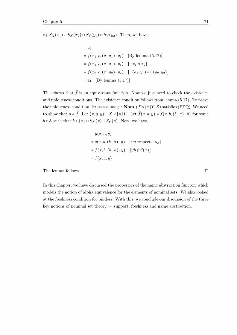
Chapter 5 71
c ∉ SX(x1) ∪ SX(x2) ∪ SY (y1) ∪ SY (y2). Then, we have,
z3
= f(x1, c, (c a1) ⋅ y1) [By lemma (5.17)]
= f(x2, c, (c a1) ⋅ y1) [∵x1 ≈ x2]
= f(x2, c, (c a2) ⋅ y2) [∵(a1, y1) ≈α (a2, y2)]
= z4 [By lemma (5.17)]
This shows that f is an equivariant function. Now we just need to check the existence
and uniqueness conditions. The existence condition follows from lemma (5.17). To prove
the uniqueness condition, let us assume g ∈ Nom (X×[A]Y,Z) satisfies (EEQ). We need
to show that g = f . Let (x, a, y) ∈ X × [A]Y . Let f(x, a, y) = f(x, b, (b a) ⋅ y) for some
b ∈ A such that b ∉ {a} ∪ SX(x) ∪ SY (y). Now, we have,
g(x, a, y)
= g(x, b, (b a) ⋅ y) [∵g respects ≈α]
= f(x, b, (b a) ⋅ y) [∵b ∉ S(x)]
= f(x, a, y)
The lemma follows.
In this chapter, we have discussed the properties of the name abstraction functor, which
models the notion of alpha equivalence for the elements of nominal sets. We also looked
at the freshness condition for binders. With this, we conclude our discussion of the three
key notions of nominal set theory — support, freshness and name abstraction.

Chapter 6
Conclusion
We have shown that a considerable portion of the theory of nominal sets can be de-
veloped constructively in the dependent type theoretic environment of Agda. We have
formalized the category theoretic properties of nominal sets, properties of freshness and
name abstraction sets as presented in [6]. This development can form the base for
future constructive implementations of nominal techniques in languages like Coq and
Agda. One of the key challenges in that direction will be the reduction of complexity of
the proofs involved. In general, machine level formalizations are much more tedious as
compared to pen and paper formalizations, since one has to work out even the smallest
technical detail explicitly. In addition to that, the thorough dependence of our work
on setoids made our proofs even more verbose, since the equivalence relation has to be
invoked at every step when working with elements of setoids. The situation becomes un-
wieldy when one has to simultaneously manipulate several setoids, which are also related
to one another. It would be interesting to find out how much of this setoid dependence
can be done away with, without yielding to non-constructive methods. For example,
if the permutations can be represented as sets instead of setoids, something which we
believe might be possible, then the verbosity of the proofs can be substantially reduced.
The other area of exploration might be looking for a minimal data type for Atom that
would satisfy all the required properties. The other problem we faced while developing
our proofs in Agda is that very often Agda fails to infer implicit arguments, thus requir-
ing one to explicitly mention all the implicit arguments, something that makes proofs
look more verbose than is necessary. If the type inference mechanism of Agda can be
made stronger, proofs will become leaner. These improvements would make large-scale
development of nominal techniques in Agda more feasible.
73

Bibliography
[1] Rod M. Burstall. Proving properties of programs by structural induction. The
computer journal, 12, 1969.
[2] N. G. de Bruijn. Lambda calculus notation with nameless dummies, a tool for
automatic formula manipulation, with applications to the church-rosser theorem.
Indagationes Mathematicae (Koninglijke Nederlandse Akademie van Wetenschap-
pen), 34(5):381–392, 1972.
[3] F. Pfenning and C. Elliot. Higher-order abstract syntax. In Proceedings of the ACM
SIGPLAN 1988 Conference on Programming Language Design and Implementation,
PLDI ’88, pages 199–208, New York, NY, USA, 1988. ACM.
[4] Furio Honsell, Marino Miculan, and Ivan Scagnetto. pi-calculus in (co)inductive
type theory. Theoretical Computer Science, 253(2):239–285, 2001.
[5] Murdoch J. Gabbay and Andrew M. Pitts. A new approach to abstract syntax with
variable binding. Formal Aspects of Computing, 13(3–5):341–363, 2002.
[6] A. M. Pitts. Nominal Sets: Names and Symmetry in Computer Science, volume 57
of Cambridge Tracts in Theoretical Computer Science. Cambridge University Press,
2013. ISBN 9781107017788.
[7] A. Swan. An Algebraic Weak Factorisation System on 01-Substitution Sets: A
Constructive Proof. ArXiv e-prints, September 2014.
[8] Mars Climate Orbiter Mishap Investigation Board. Mars Climate Orbiter Mishap
Investigation Board Phase I Report, November 1999.
[9] U.S.-Canada Power System Outage Task Force. Final Report on the August 14,
2003 Blackout in the United States and Canada: Causes and Recommendations,
April 2004.
[10] Edsger Wybe Dijkstra. A Discipline of Programming. Prentice Hall PTR, Upper
Saddle River, NJ, USA, 1st edition, 1997.
75
Bibliography 76
[11] Daniel Hirschkoff. A full formalisation of π-calculus theory in the calculus of con-
structions. In ElsaL. Gunter and Amy Felty, editors, Theorem Proving in Higher
Order Logics, volume 1275 of Lecture Notes in Computer Science, pages 153–169.
Springer Berlin Heidelberg, 1997.
[12] BrianE. Aydemir, Aaron Bohannon, Matthew Fairbairn, J.Nathan Foster, Ben-
jaminC. Pierce, Peter Sewell, Dimitrios Vytiniotis, Geoffrey Washburn, Stephanie
Weirich, and Steve Zdancewic. Mechanized metatheory for the masses: The
poplmark challenge. In Joe Hurd and Tom Melham, editors, Theorem Proving
in Higher Order Logics, volume 3603 of Lecture Notes in Computer Science, pages
50–65. Springer Berlin Heidelberg, 2005.
[13] Mark Ross Shinwell. The Fresh Approach: Functional Programming with Names
and Binders. PhD thesis, University of Cambridge, 2005.
[14] Christian Urban and Stefan Berghofer. A recursion combinator for nominal
datatypes implemented in isabelle/hol. In Ulrich Furbach and Natarajan Shankar,
editors, IJCAR, volume 4130 of Lecture Notes in Computer Science, pages 498–512.
Springer, 2006.
[15] Brian Aydemir, Aaron Bohannon, and Stephanie Weirich. Nominal reasoning tech-
niques in coq: (extended abstract). Electronic Notes in Theoretical Computer Sci-
ence, 174(5):69 – 77, 2007.
[16] R. Zach. Hilbert’s program then and now. In Dale Jacquette, ed., Philosophy of
Logic, volume 5 of Handbook of the Philosophy of Science, pages 411–417, Amster-
dam, 2006. Elsevier.
[17] L. E. J. Brouwer. Philosophy and Foundations of Mathematics. Collected Works,
Volume-1. North-Holland Pub. Co., 1975.
[18] A. Heyting. Intuitionism: an introduction. Studies in logic and the foundations of
mathematics. North-Holland Pub. Co., 1971.
[19] P. Martin-Lof. Constructive mathematics and computer programming. In Proc.
Of a Discussion Meeting of the Royal Society of London on Mathematical Logic
and Programming Languages, pages 167–184, Upper Saddle River, NJ, USA, 1985.
Prentice-Hall, Inc.
[20] Per Martin-Lof. An intuitionistic theory of types, 1972.
[21] B. Russell. Mathematical logic as based on the theory of types. American Journal
of Mathematics, 30:222–262, 1908.
Bibliography 77
[22] A. Church. A formulation of a simple theory of types. Journal of Symbolic Logic,
5:56–68, 1940.
[23] Jean Yves Girard. Interpretation fonctionelle et elimination des coupures dans
l’arithmetique d’ordre superieur. PhD thesis, Universite Paris VII, 1972.
[24] Nicolas Oury and Wouter Swierstra. The power of pi. In Proceedings of the 13th
ACM SIGPLAN International Conference on Functional Programming, ICFP ’08,
pages 39–50, New York, NY, USA, 2008. ACM.
[25] Bengt Nordstrom, Kent Petersson, and Jan M. Smith. Programming in Martin-
Lof ’s Type Theory: An Introduction. Oxford University Press, 1990.
[26] Ulf Norell. Towards a practical programming language based on dependent type
theory. PhD thesis, Department of Computer Science and Engineering, Chalmers
University of Technology, SE-412 96 Goteborg, Sweden, September 2007.
[27] Ulf Norell. Dependently typed programming in agda. In Pieter Koopman, Rinus
Plasmeijer, and Doaitse Swierstra, editors, Advanced Functional Programming, vol-
ume 5832 of Lecture Notes in Computer Science, pages 230–266. Springer Berlin
Heidelberg, 2009.
[28] Martin Hofmann. Extensional Concepts in Intensional Type Theory. PhD thesis,
University of Edinburgh, Scotland , UK, July 1995.
[29] Steve Awodey. Category theory, volume 49 of Oxford Logic Guides. The Clarendon
Press Oxford University Press, New York, 2006.
[30] S. Eilenberg and Saunders Mac Lane. General theory of natural equivalences. Trans.
Am. Math. Soc., 58:231–294, 1945.
[31] Peter Freyd. Algebraically complete categories. In Aurelio Carboni, MariaCristina
Pedicchio, and Guiseppe Rosolini, editors, Category Theory, volume 1488 of Lecture
Notes in Mathematics, pages 95–104. Springer Berlin Heidelberg, 1991.
[32] Andrew M. Pitts. Alpha-structural recursion and induction. J. ACM, 53(3):459–
506, May 2006.


![Practical introduction to Agda - ERDI Gergo · Introduction \Agda is a proof assistant [...] for developing constructive proofs based on the Curry-Howard correspondence [...]. It](https://img.pdfslide.us/doc/110x75/605ad1ca8390d946b912f53a/practical-introduction-to-agda-erdi-gergo-introduction-agda-is-a-proof-assistant.jpg)