Constructive cooperative coevolution for large-scale ...publications.lib.chalmers.se/records/fulltext/253271/local_253271.pdfConstructive cooperative coevolution for large-scale

J Heuristics (2017) 23:449–469DOI 10.1007/s10732-017-9351-z

Constructive cooperative coevolution for large-scaleglobal optimisation

Emile Glorieux1 · Bo Svensson1 · Fredrik Danielsson1 ·Bengt Lennartson2

Received: 25 March 2016 / Revised: 29 June 2017 / Accepted: 30 June 2017 /Published online: 17 July 2017© The Author(s) 2017. This article is an open access publication

Abstract This paper presents theConstructiveCooperativeCoevolutionary (C3) algo-rithm, applied to continuous large-scale global optimisation problems. The noveltyof C3 is that it utilises a multi-start architecture and incorporates the CooperativeCoevolutionary algorithm. The considered optimisation problem is decomposed intosubproblems. An embedded optimisation algorithm optimises the subproblems sep-arately while exchanging information to co-adapt the solutions for the subproblems.Further,C3 includes anovel constructive heuristic that generates different feasible solu-tions for the entire problem and thereby expedites the search. In thiswork, two differentversions of C3 are evaluated on high-dimensional benchmark problems, including theCEC’2013 test suite for large-scale global optimisation. C3 is compared with severalstate-of-the-art algorithms, which shows that C3 is among the most competitive algo-rithms. C3 outperforms the other algorithms for most partially separable functionsand overlapping functions. This shows that C3 is an effective algorithm for large-scaleglobal optimisation. This paper demonstrates the enhanced performance by usingconstructive heuristics for generating initial feasible solutions for Cooperative Coevo-lutionary algorithms in a multi-start framework.

Keywords Evolutionary optimisation · Cooperative coevolution · Algorithm designand analysis · Large-scale optimisation

This work was supported in part by Västra Götalandsregionen, Sweden, under the Grant PROSAM612-0974-14.

B Emile [email protected]

1 Department of Engineering Science, University West, S-461 86 Trollhättan, Sweden

2 Department of Signals and Systems, Chalmers University of Technology, S-412 96 Gothenburg,Sweden

123

http://crossmark.crossref.org/dialog/?doi=10.1007/s10732-017-9351-z&domain=pdf

http://orcid.org/0000-0002-0044-2795

450 E. Glorieux et al.

1 Introduction

Manypractical real-world optimisationproblemswithin engineering canbe consideredas global optimisation problems. Such problems are also often complex and large-scale(i.e. large number of parameters) which makes them difficulty to solve (Ali et al. 2005;Lozano et al. 2011). Heuristics and metaheuristics are among the existing methods tosolve continuous optimisation problems.

Multi-start methods are one type of metaheuristics. These methods usually embedother optimisation algorithms, such as local search and neighbourhood search, whichlack the required diversification to explore the search space globally (Grendreau andPotvin 2010). Themulti-start method starts the embedded algorithm frommultiple dif-ferent initial solutions, often obtained by random sampling. A well-known multi-startmethod, the Continuous Greedy Randomised Adaptive Search Procedure (CGRASP)(Hirsch et al. 2010), is relevant for the work presented in this paper.

Another metaheuristic, that is adopted in this work, is the Cooperative Coevolu-tionary (CC) algorithm (Potter and De Jong 1994). This algorithm requires that theoptimisation problem is decomposed into subproblems. Then, each subproblem hasa group of corresponding parameters. These subproblems are optimised separately,but there is cooperation between the optimisations. The cooperation is necessary toensure that the solutions for the subproblems are still optimal when combined into asolution for the entire problem. CC has a good performance especially on large-scaleoptimisation problems. Though, other works (Li and Yao 2009; Omidvar et al. 2014,2010; Potter and De Jong 1994; Ray and Yao 2009; Yang et al. 2008) found thatthe CC struggles to solve non-separable problems (i.e. interactions/interdependenciesbetween parameters). Those works propose different versions of CC to improve theperformance on non-separable problems. These different versions of CCmainly focuson regrouping the parameters into different subproblems. The aimwith this is to gatherinteracting parameters in the same subproblem and optimise them together.

This work considers a different approach to improve CC’s performance, but canstill be used together with earlier proposed regrouping strategies. The focus is onextending CC using the GRASP multi-start architecture. The algorithm proposed inthis work is called the Constructive Cooperative Coevolutionary (C3) algorithm. Aconstructive heuristic is incorporated in C3 to efficiently find good feasible solutions.These feasible solutions are used as initial solution for CC. When the search of CCstagnates, C3 restarts the constructive heuristic to get a new initial solution. C3’saim is to increase the performance of CC, specifically on non-separable large-scaleoptimisation problems.

The main contribution of this paper is the evaluation of the performance and therobustness of the C3 algorithm and to get insight into its behaviour towards spe-cific characteristics of large-scale optimisation problems (modality, separability, etc.).Compared to previous work (Glorieux et al. 2014, 2015), C3 is improved in order tomake it scalable in number of subproblems. Thereby, it can be applied on awider rangeof problems. C3 is compared with other algorithms, such as the Cooperative Coevolu-tionary (CC) algorithm (Potter and De Jong 2000; Wiegand et al. 2001; Zamuda et al.2008), Self-Adaptive Differential Evolution (jDErpo) (Brest et al. 2014) and Particle

123

Constructive cooperative coevolution for large-scale... 451

Swarm Optimiser (PSO) (Nickabadi et al. 2011). This shows that C3 is better than theother algorithms, both in terms of performance and robustness.

The remaining of this paper is organised as follows, in Sect. 2 the relevant back-ground information for C3 is given. In Sect. 3, the details of C3 are presented. Theimplementation of the tests performed in this paper is described in Sect. 4. The resultsof these tests are presented and discussed in Sect. 5 and finally Sect. 6 concludes thiswork.

2 Background

In earlier work, C3 is applied on practical optimisation problems concerning controlof interacting production stations (Glorieux et al. 2014, 2015). There, it is used withina simulation-based optimisation framework and it is shown that C3 outperforms otheroptimisation methods. The previous version of C3 was not scalable in number ofsubproblems, which was a limitation of the algorithm. In this work, an improvedversion of C3 is proposed for which this limitation is removed. Hence, it can beapplied on a wider range of problems. In previous work on C3 the algorithm has onlybeen tested on problems that has up to 100 dimensions. In this work, C3 is tested on awide range of large-scale problems with up to 1000 dimensions. This section providesthe relevant background for the design of C3.

2.1 Greedy randomised adaptive search procedure

A well-known multi-start method (Martí et al. 2010) is the Continuous Greedy Ran-domised Adaptive Search Procedure (CGRASP) (Hirsch et al. 2007, 2010), which isbased on the discrete GRASP (Feo and Resende 1995). For each start (also referred toas iteration), two phases are executed: a constructive phase and a local improvementphase. The constructive phase builds a feasible solution. This is done by performinga line search separately in each search direction while keeping the parameters for theother directions fixed to a random initial value. This solution is then used as an initialsolution for the optimisation algorithm used in the local improvement phase. The localimprovement phase terminates when the search reaches a local optimum.

Hirsch et al. (2007, 2010) evaluated the performance of CGRASP on a set of stan-dard benchmark functions and a real world continuous optimisation problems. Forsome of the benchmark functions, CGRASP’s performance was not as good com-pared to other optimisation methods (Simulated Annealing and Tabu Search). Later,an improved version of DC-GRASP was proposed by Araújo et al. (2015) that has animproved performance, especially on high-dimensional problems.

C3 adopts CGRASP’s multi-start architecture with a constructive and improvementphase for each start. The constructive phase of C3 is different in that the subproblemsare stepwise optimised (instead of a single parameter) and only the previously opti-mised subproblems are kept fixed and the other subproblems are not considered duringthe function evaluations. Another difference is that in C3’s improvement phase CC isincorporated.

123


2.2 Cooperative coevolutionary algorithm

The Cooperative Coevolutionary (CC) algorithm for continuous global function opti-misationwas first proposed byPotter andDe Jong (1994). It requires that the problem isdecomposed into subproblems. Typically, a natural decomposition is used that groupsthe D parameters into n sets, one set for each subproblem. For each subproblem, asubpopulation is initialised and optimised separately. In order to evaluate the cost of amember of a subpopulation, collaborator solutions are selected from the other subpop-ulations in order to form a complete solution. The combination of these collaboratorsis called the context solution. These collaborators are updated at specific intervals.

It has been proposed to use multiple collaborators from each subpopulation (Potterand De Jong 1994;Wiegand et al. 2001). When multiple collaborators are used, differ-ent combinations of these collaborators are evaluated to calculate the cost for a givensubpopulation member. The function evaluation results of these different combina-tions are then combined into a single cost value for the subpopulation member. One ofthe questions when using CC is how to select the collaborators for the context solutionand how many from each subpopulation.Wiegand et al. (2001) investigate the choiceof the collaborator solutions, more specifically the collaborator selection pressure, thenumber of collaborators for a given function evaluation, and the credit assignmentwhen using multiple collaborators. It was shown that how to select the collaboratorsdepends on specific characteristics of the problem, especially the separability. More-over, the selection pressure of collaborators is of less importance than the number ofcollaborators.Although, increasing the number of collaborators is not always preferredbecomes the cost calculation because computationally more expensive.

The decomposition or grouping of the parameters influences the performance ofthe cooperative coevolutionary algorithm. Random grouping has been proposed toincrease the performance on non-separable high dimensional problems (Omidvaret al. 2010; Yang et al. 2008). With random grouping, the parameters are frequentlyregrouped to increase the chance of having interacting parameters in the same sub-problem. Omidvar et al. (2014) propose differential grouping to automatically uncoverthe underlying substructures of the problem for grouping the parameters. The param-eter groups are then determined so that the interactions between the subproblems iskept to a minimum. Results show that this increases the performance significantlyfor non-separable problems. Ray and Yao (2009) propose to group the parametersaccording to their observed correlation during the optimisation. With this approach, apopulation of solutions for the entire problem is generated, prior to the optimisation,to determine the initial grouping. Thus, it requires an additional computational effort.Decomposition strategies for C3 are not investigated in the work presented in thispaper but is considered a topic for future studies.

CC could have the tendency to limit its search to a single neighbourhood instead ofexploring the search spacemore (Grendreau andPotvin 2010). This behaviour has beenobserved especially when best solution in the subpopulation is used as collaborator.The search then convergence towards a local optimum.

Shi et al. (2005) propose using Differential Evolution (DE) instead of a geneticalgorithm for the subproblem optimisations in the cooperative coevolutionary algo-rithm. Furthermore, an alternative static decomposition scheme is proposed in which

123


a subproblem takes half of the parameters. Typically, a problem is decomposed sothat there is a subproblem for each parameter. The proposed algorithm (CCDE) anddecomposition scheme showed an improved performance compared to DE and com-pared to the typical decomposition scheme. Though, the proposed algorithm was nottested on large scale non-separable problems.

Using the Particle Swarm Optimiser (PSO) for the subproblem optimisation in CChas been proposed by Bergh and Engelbrecht (2004). CCPSO has an increased perfor-mance and robustness compared to PSO, especially when the optimisation problem’sdimension increases. Though, itwas also noticed that the chance of converging to a sub-optimum increases. Li and Yao (2012) propose a more advanced version of CCPSOthat incorporates a new PSO model and a random parameter regrouping scheme withdynamic size for large scale problems up to 2000 parameters. The results showedan increased performance compared to PSO and other state-of-the-art optimisationalgorithms.

3 Constructive cooperative coevolutionary algorithm

The details of the Constructive Cooperative Coevolutionary (C3) algorithm aredescribed in this section. In Algorithm 1 the pseudo code of C3 is presented. C3

is based on CGRASP’s construction and adopts the multi-start architecture. Further-more, C3 also incorporates the CC algorithm. Hence, each iteration (or start) of C3

includes a constructive heuristic (Phase I) and CC (Phase II).The optimisation problem is decomposed into n subproblems. This is done by

partitioning the D-dimensional set of search dimensions G = {1, 2, . . . , D} into nsetsG1, . . . ,Gn (line 1 in Algorithm 1). The decomposition or partitioning G can havean influence on the performance of C3 and is thus important. This is not investigatedfurther in this work, but suggested as future work. The problems in this work arealways decomposed randomly in equal sized subproblems.

In Phase I, the constructive heuristic builds up a feasible solution for the entire opti-misation problem (xi t,constr on line 4 in Algorithm 1). A feasible solution is a solutionthat does not violate the constraints of the optimisation problem. Next, xi t,constr isused in Phase II as initial context solution for CC that further improves this solution(line 5 in Algorithm 1). Phase II is terminated when CC’s search stagnates. At thenext iteration, i t + 1, the constructive heuristic (Phase I) is restarted to build up anew feasible solution. This is repeated for all iterations until the termination criteriaare met. An example of a termination criterion is to limit the maximum number offunction evaluations. The best solution x∗ found over all iterations is recorded andpresented as the result when the optimisation ends.

In both Phase I and II, the subproblems are optimised separately during n steps,by an embedded optimisation algorithm. To calculate the cost of the members duringPhase I, the subproblems’ trial solutions are assembled in a partial solution. A partialsolution pi from Step i , is a solution for the first i subproblems, with 1 ≤ i ≤ n,and neglects Subproblem i + 1 to Subproblem n. During the function evaluation, theneglected subproblems are then also not considered. Note that calculating the cost of apartial solution is equivalent to calculating the cost of a solution for a smaller problemthat only considers the parameters that are included in the partial solution.

123


During Phase II, to calculate the cost of a member of a subpopulation, they areassembled in a context solution (a solution for the entire problem) in the same way aswith CC. Asmentioned earlier, the context solution consists of collaborators, one fromeach of the other subpopulations. In this work, different collaborators are randomlychosen for each function evaluation.

The embedded optimisation algorithmmust be a population-based algorithm.Whenit is deployed for optimising a subproblem, it initialises a (sub)population for thecorresponding subproblem’s parameters and evolves this subpopulation according tothe procedure of the used population-based algorithm. After the optimisation, the bestpartial solutions in this subpopulations are used while the others are discarded. Hence,in general terms, C3 can be combined with any suitable population-based optimisationalgorithm. This is demonstrated in this work by using both an evolution algorithm (i.e.Differential Evolution) and a swarm-based algorithm (i.e. Particle Swarm Optimiser).

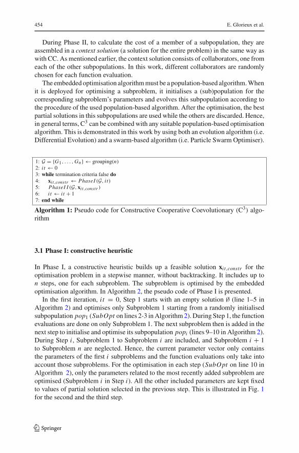
1: G = {G1, . . . ,Gn} ← grouping(n)2: i t ← 03: while termination criteria false do4: xi t,constr ← PhaseI (G, i t)5: PhaseI I (G, xi t,constr )6: i t ← i t + 17: end while

Algorithm 1: Pseudo code for Constructive Cooperative Coevolutionary (C3) algo-rithm

3.1 Phase I: constructive heuristic

In Phase I, a constructive heuristic builds up a feasible solution xi t,constr for theoptimisation problem in a stepwise manner, without backtracking. It includes up ton steps, one for each subproblem. The subproblem is optimised by the embeddedoptimisation algorithm. In Algorithm 2, the pseudo code of Phase I is presented.

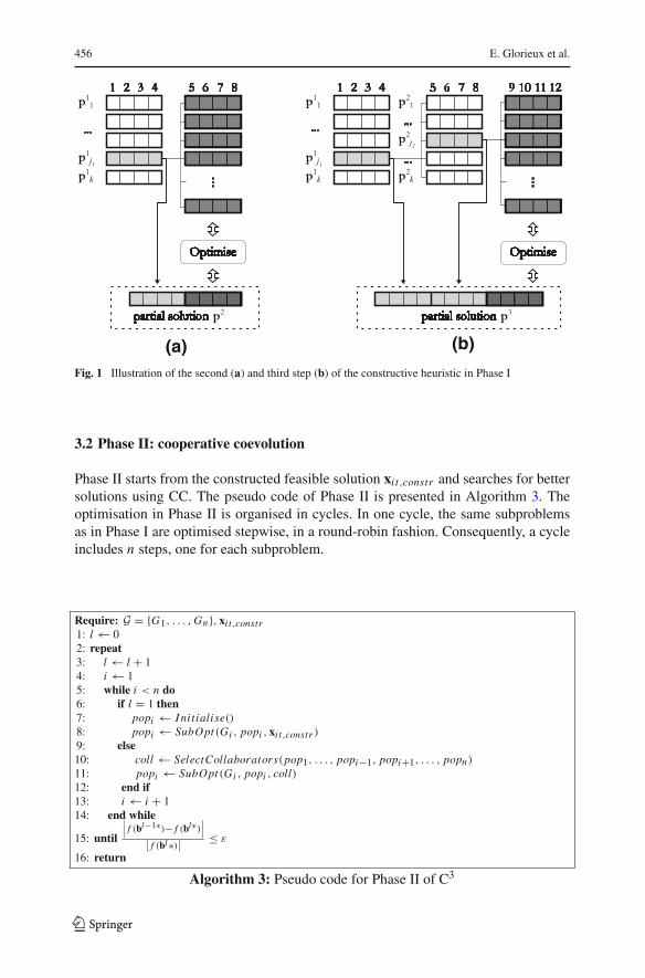
In the first iteration, i t = 0, Step 1 starts with an empty solution ∅ (line 1–5 inAlgorithm 2) and optimises only Subproblem 1 starting from a randomly initialisedsubpopulation pop1 (SubOpt on lines 2-3 inAlgorithm2). During Step 1, the functionevaluations are done on only Subproblem 1. The next subproblem then is added in thenext step to initialise and optimise its subpopulation popi (lines 9–10 in Algorithm 2).During Step i , Subproblem 1 to Subproblem i are included, and Subproblem i + 1to Subproblem n are neglected. Hence, the current parameter vector only containsthe parameters of the first i subproblems and the function evaluations only take intoaccount those subproblems. For the optimisation in each step (SubOpt on line 10 inAlgorithm 2), only the parameters related to the most recently added subproblem areoptimised (Subproblem i in Step i). All the other included parameters are kept fixedto values of partial solution selected in the previous step. This is illustrated in Fig. 1for the second and the third step.

123


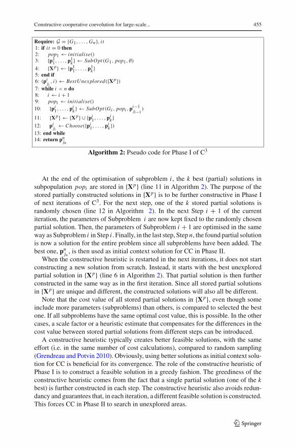
Require: G = {G1, . . . ,Gn}, i t1: if i t = 0 then2: pop1 ← ini tialise()3: {p11, . . . ,p1k } ← SubOpt (G1, pop1,∅)

4: {Xp} ← {p11, . . . , p1k }5: end if6: (piji , i) ← BestUnexplored({Xp})7: while i < n do8: i ← i + 19: popi ← ini tialise()10: {pi1, . . . , pik } ← SubOpt (Gi , popi , p

i−1ji−1

)

11: {Xp} ← {Xp} ∪ {pi1, . . . ,pik }12: piji ← Choose({pi1, . . . , pik })13: end while14: return pnjn

Algorithm 2: Pseudo code for Phase I of C3

At the end of the optimisation of subproblem i , the k best (partial) solutions insubpopulation popi are stored in {Xp} (line 11 in Algorithm 2). The purpose of thestored partially constructed solutions in {Xp} is to be further constructive in Phase Iof next iterations of C3. For the next step, one of the k stored partial solutions israndomly chosen (line 12 in Algorithm 2). In the next Step i + 1 of the currentiteration, the parameters of Subproblem i are now kept fixed to the randomly chosenpartial solution. Then, the parameters of Subproblem i + 1 are optimised in the sameway as Subproblem i in Step i . Finally, in the last step, Step n, the found partial solutionis now a solution for the entire problem since all subproblems have been added. Thebest one, pnjn , is then used as initial context solution for CC in Phase II.

When the constructive heuristic is restarted in the next iterations, it does not startconstructing a new solution from scratch. Instead, it starts with the best unexploredpartial solution in {Xp} (line 6 in Algorithm 2). That partial solution is then furtherconstructed in the same way as in the first iteration. Since all stored partial solutionsin {Xp} are unique and different, the constructed solutions will also all be different.

Note that the cost value of all stored partial solutions in {Xp}, even though someinclude more parameters (subproblems) than others, is compared to selected the bestone. If all subproblems have the same optimal cost value, this is possible. In the othercases, a scale factor or a heuristic estimate that compensates for the differences in thecost value between stored partial solutions from different steps can be introduced.

A constructive heuristic typically creates better feasible solutions, with the sameeffort (i.e. in the same number of cost calculations), compared to random sampling(Grendreau and Potvin 2010). Obviously, using better solutions as initial context solu-tion for CC is beneficial for its convergence. The role of the constructive heuristic ofPhase I is to construct a feasible solution in a greedy fashion. The greediness of theconstructive heuristic comes from the fact that a single partial solution (one of the kbest) is further constructed in each step. The constructive heuristic also avoids redun-dancy and guarantees that, in each iteration, a different feasible solution is constructed.This forces CC in Phase II to search in unexplored areas.

123


(a) (b)

Fig. 1 Illustration of the second (a) and third step (b) of the constructive heuristic in Phase I

3.2 Phase II: cooperative coevolution

Phase II starts from the constructed feasible solution xi t,constr and searches for bettersolutions using CC. The pseudo code of Phase II is presented in Algorithm 3. Theoptimisation in Phase II is organised in cycles. In one cycle, the same subproblemsas in Phase I are optimised stepwise, in a round-robin fashion. Consequently, a cycleincludes n steps, one for each subproblem.

Require: G = {G1, . . . ,Gn}, xi t,constr1: l ← 02: repeat3: l ← l + 14: i ← 15: while i < n do6: if l = 1 then7: popi ← I ni tialise()8: popi ← SubOpt (Gi , popi , xi t,constr )9: else10: coll ← SelectCollaborators(pop1, . . . , popi−1, popi+1, . . . , popn)

11: popi ← SubOpt (Gi , popi , coll)12: end if13: i ← i + 114: end while

15: until

∣∣∣ f (bl−1∗)− f (bl∗)

∣∣∣

∣∣ f (bl∗)

∣∣

≤ ε

16: return

Algorithm 3: Pseudo code for Phase II of C3

123


Subpopulation popi is optimised in the corresponding Step i by the embeddedoptimisation algorithm (line 11 in Algorithm 3). To evaluate the cost, an individual ofthe subpopulation is assembled in a context solution to form a complete solution. Thiscontext solution consists of collaborator solutions that are randomly chosen from theother subpopulations (line 10 in Algorithm 3). For each function evaluation, differentcollaborators are randomly selected as proposed by Wiegand et al. (2001).

During the first cycle of Phase II the context solution is initially the constructedsolution xi t,constr instead of collaborators from the other subpopulations (lines 6–9in Algorithm 3). A collaborator from subpopulation popi of Subproblem i is usedonly after Step i has been completed. In other words, in Step i , the collaborators forSubproblem i + 1 until Subproblem n are taken from xit,constr . Only in the first cycle,the subpopulations are randomly initialised at the start of the subproblem optimisation(line 7 in Algorithm 3).

Phase II is terminated when the search stagnates because it is likely that then alocal optimum is reached. When the relative difference between the best solutionfound during the current cycle and the best solution from the previous cycle is lessthan ε, Phase II is terminated. This is shown in line 15 in Algorithm 3, where bl∗ isthe best solution found in cycle l.

Because CC optimises the smaller subproblems separately, it is well-suited forlarge-scale problems. The context solution ensures that a subproblem is co-adaptivelyoptimised, as a part of the complete problem, and not as an isolated optimisation prob-lem. By using different collaborators in the context solution for each cost calculation,a subproblem is optimised to collaborate with the individuals of the other subpopula-tions and not with just a single specific context solution. On the other hand, using theconstructed solution from Phase I as context solution in the first cycle ensures that theCC starts search in the region of the search space specific by this constructed solution.In each iteration, the constructed solution directs CC to search a different region ofthe search space.

4 Implementation

Two version of C3, C3jDErpo and C3PSO, are compared with 4 other algorithms. The6 different optimisation algorithms compared in this work are: C3jDErpo, CCjDErpo,jDErpo, C3PSO, CCPSO, PSO. Here, C3jDErpo refers to C3 where jDErpo is used asembedded algorithm to optimise the subproblems, and in the sameway for CCjDErpo,C3PSO and CCPSO. To evaluate the performance and robustness of C3, 51 tests onlarge-scale benchmark functions were done for both versions of C3. Of which, 36 arebased on 12 benchmark functions (see Table 1 and Appendix 1) and each is tested with3 different number of dimensions (D = 100, D = 500, D = 1000). Additionally,tests are done on the test suite of the CEC’2013 special session on Large-Scale GlobalOptimisation (LSGO) (Li et al. 2013).

The jDErpo algorithmused as an embedded algorithm inC3jDErpo for the subprob-lem optimisation is proposed by Brest et al. (2014), and has a self-adaptive mechanismto tune the control parameters, i.e. the mutation scale factor (F) and the crossoverparameter (CR). The PSO algorithm used as an embedded algorithm in C3PSO for

123


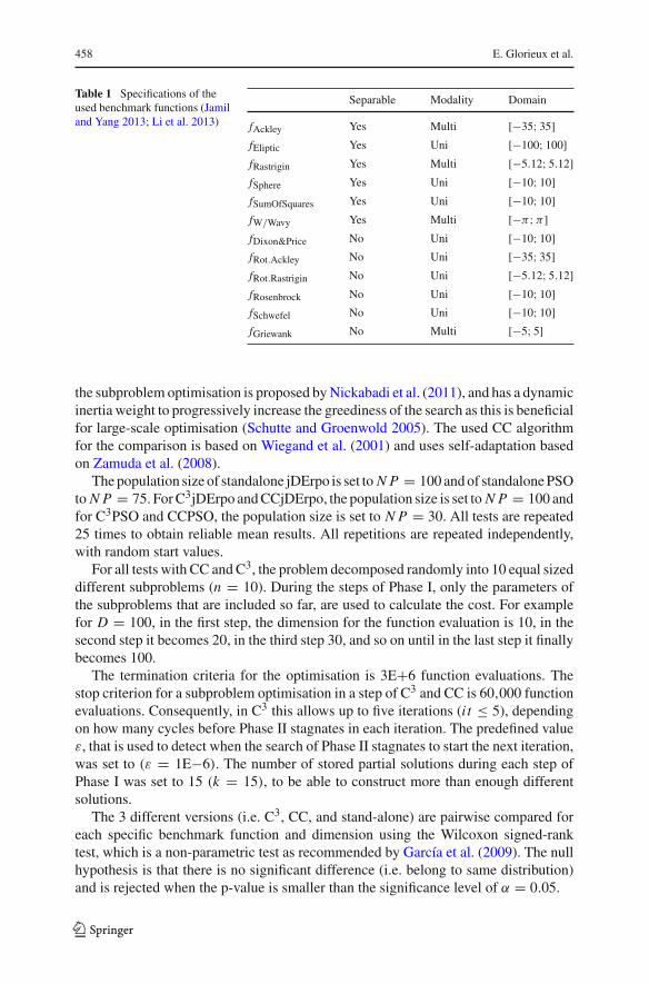
Table 1 Specifications of theused benchmark functions (Jamiland Yang 2013; Li et al. 2013)

Separable Modality Domain

fAckley Yes Multi [−35; 35]fEliptic Yes Uni [−100; 100]fRastrigin Yes Multi [−5.12; 5.12]fSphere Yes Uni [−10; 10]fSumOfSquares Yes Uni [−10; 10]fW/Wavy Yes Multi [−π;π ]fDixon&Price No Uni [−10; 10]fRot.Ackley No Uni [−35; 35]fRot.Rastrigin No Uni [−5.12; 5.12]fRosenbrock No Uni [−10; 10]fSchwefel No Uni [−10; 10]fGriewank No Multi [−5; 5]

the subproblem optimisation is proposed byNickabadi et al. (2011), and has a dynamicinertia weight to progressively increase the greediness of the search as this is beneficialfor large-scale optimisation (Schutte and Groenwold 2005). The used CC algorithmfor the comparison is based on Wiegand et al. (2001) and uses self-adaptation basedon Zamuda et al. (2008).

Thepopulation size of standalone jDErpo is set to N P = 100 andof standalonePSOto N P = 75. ForC3jDErpo andCCjDErpo, the population size is set to N P = 100 andfor C3PSO and CCPSO, the population size is set to N P = 30. All tests are repeated25 times to obtain reliable mean results. All repetitions are repeated independently,with random start values.

For all tests with CC and C3, the problem decomposed randomly into 10 equal sizeddifferent subproblems (n = 10). During the steps of Phase I, only the parameters ofthe subproblems that are included so far, are used to calculate the cost. For examplefor D = 100, in the first step, the dimension for the function evaluation is 10, in thesecond step it becomes 20, in the third step 30, and so on until in the last step it finallybecomes 100.

The termination criteria for the optimisation is 3E+6 function evaluations. Thestop criterion for a subproblem optimisation in a step of C3 and CC is 60,000 functionevaluations. Consequently, in C3 this allows up to five iterations (i t ≤ 5), dependingon how many cycles before Phase II stagnates in each iteration. The predefined valueε, that is used to detect when the search of Phase II stagnates to start the next iteration,was set to (ε = 1E−6). The number of stored partial solutions during each step ofPhase I was set to 15 (k = 15), to be able to construct more than enough differentsolutions.

The 3 different versions (i.e. C3, CC, and stand-alone) are pairwise compared foreach specific benchmark function and dimension using the Wilcoxon signed-ranktest, which is a non-parametric test as recommended by García et al. (2009). The nullhypothesis is that there is no significant difference (i.e. belong to same distribution)and is rejected when the p-value is smaller than the significance level of α = 0.05.

123


5 Results and discussion

In this section, the results of the performed tests in this work are presented and therelevant aspects of the results are highlighted and discussed. For simplicity, in this sec-tion C3 is used as a collective name for C3jDErpo and C3PSO, and CC for CCjDErpoand CCPSO, and the “stand-alone algorithms” for jDErpo and PSO.

5.1 Convergence analysis

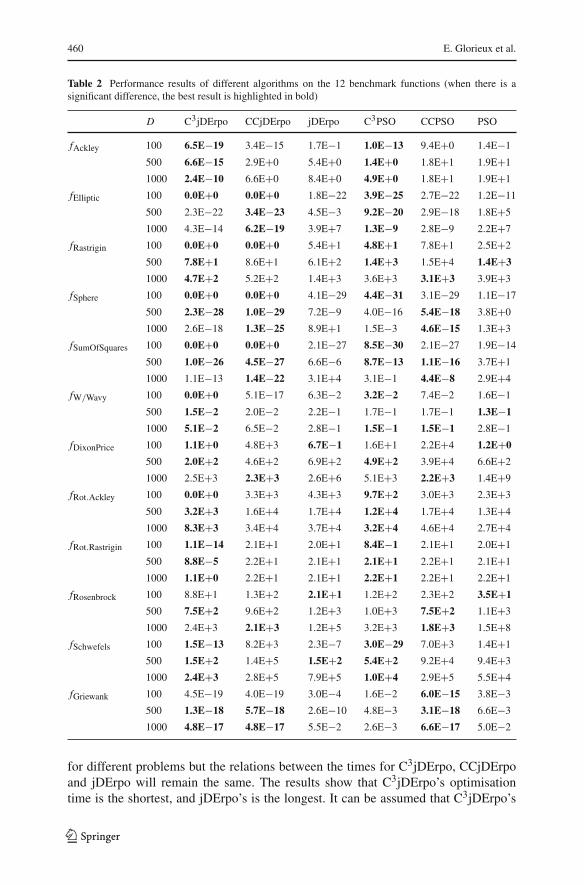
The evaluation of C3’s convergence performance is presented in this section. Themain indicator for this is the cost of the best solution found after all 3E + 6 functionevaluations. The results are shown in Table 2. These are the mean of 25 independentrepetitions. When there is a significant difference between the algorithms accordingto the pairwise comparison using the Wilcoxon signed-rank test, the best result(s) arehighlighted in bold font in Table 2.

It can be seen that C3 has a better convergence for themajority of the tests comparedto CC and the stand-alone algorithms. Considering the statistically significant differ-ences, C3jDErpo is the best algorithm or among the best in 28 of the 36 tests comparedto CCjDErpo and jDErpo, and C3PSO in 23 of the 36 tests compared to CCPSO andPSO. Furthermore, the pairwise comparison showed that C3jDErpo performs betterthan CCjDErpo in 20 of the 36 tests, and similar in 10. C3PSO performs better in 20 ofthe 36 tests, and similar in 5 tests. There is also no drastic deterioration in convergenceperformance when the number of dimensions increases. It can be concluded that ingeneral there is a benefit of using C3 instead of CC because it either performs better orat least similar. It must be noted that C3’s convergence performance is better than CCon the non-separable functions, except for fRosenbrock. This indicates that C3 strugglesless with this type of optimisation problems.

The pairwise comparison between C3 and the standalone algorithms showed thatC3jDErpo performs significantly better in 33 of the 36 tests compared with jDErpo,and C3PSO performs significantly better in 31 of the 36 tests. It can be concludedthat C3 performs better on these large-scale problems compared to the stand-alonealgorithms.

It can be concluded that in general C3jDErpo shows the best convergence perfor-mance compared with C3PSO. The same is true for CCjDErpo and CCPSO, and alsowhen comparing jDErpo and PSO. Note that the embedded optimisation algorithmfor the subproblem optimisations has a significant influence on the convergence ofC3. If the subproblems have very different characteristics, it might be valuable to evenconsider different optimisation algorithms for specific subproblems.

5.2 Computational effort

The difference in computation effort ofC3, CCand a stand-alone algorithm is analysed.This was done by recording the optimisation time on the Rosenbrock benchmarkfunction ( fRosenbrock) and with jDErpo. The results of this are presented in Table 3.Each test was repeated 25 times on the same computer. The specific time values differ

123


Table 2 Performance results of different algorithms on the 12 benchmark functions (when there is asignificant difference, the best result is highlighted in bold)

D C3jDErpo CCjDErpo jDErpo C3PSO CCPSO PSO

fAckley 100 6.5E−19 3.4E−15 1.7E−1 1.0E−13 9.4E+0 1.4E−1

500 6.6E−15 2.9E+0 5.4E+0 1.4E+0 1.8E+1 1.9E+1

1000 2.4E−10 6.6E+0 8.4E+0 4.9E+0 1.8E+1 1.9E+1

fElliptic 100 0.0E+0 0.0E+0 1.8E−22 3.9E−25 2.7E−22 1.2E−11

500 2.3E−22 3.4E−23 4.5E−3 9.2E−20 2.9E−18 1.8E+5

1000 4.3E−14 6.2E−19 3.9E+7 1.3E−9 2.8E−9 2.2E+7

fRastrigin 100 0.0E+0 0.0E+0 5.4E+1 4.8E+1 7.8E+1 2.5E+2

500 7.8E+1 8.6E+1 6.1E+2 1.4E+3 1.5E+4 1.4E+3

1000 4.7E+2 5.2E+2 1.4E+3 3.6E+3 3.1E+3 3.9E+3

fSphere 100 0.0E+0 0.0E+0 4.1E−29 4.4E−31 3.1E−29 1.1E−17

500 2.3E−28 1.0E−29 7.2E−9 4.0E−16 5.4E−18 3.8E+0

1000 2.6E−18 1.3E−25 8.9E+1 1.5E−3 4.6E−15 1.3E+3

fSumOfSquares 100 0.0E+0 0.0E+0 2.1E−27 8.5E−30 2.1E−27 1.9E−14

500 1.0E−26 4.5E−27 6.6E−6 8.7E−13 1.1E−16 3.7E+1

1000 1.1E−13 1.4E−22 3.1E+4 3.1E−1 4.4E−8 2.9E+4

fW/Wavy 100 0.0E+0 5.1E−17 6.3E−2 3.2E−2 7.4E−2 1.6E−1

500 1.5E−2 2.0E−2 2.2E−1 1.7E−1 1.7E−1 1.3E−1

1000 5.1E−2 6.5E−2 2.8E−1 1.5E−1 1.5E−1 2.8E−1

fDixonPrice 100 1.1E+0 4.8E+3 6.7E−1 1.6E+1 2.2E+4 1.2E+0

500 2.0E+2 4.6E+2 6.9E+2 4.9E+2 3.9E+4 6.6E+2

1000 2.5E+3 2.3E+3 2.6E+6 5.1E+3 2.2E+3 1.4E+9

fRot.Ackley 100 0.0E+0 3.3E+3 4.3E+3 9.7E+2 3.0E+3 2.3E+3

500 3.2E+3 1.6E+4 1.7E+4 1.2E+4 1.7E+4 1.3E+4

1000 8.3E+3 3.4E+4 3.7E+4 3.2E+4 4.6E+4 2.7E+4

fRot.Rastrigin 100 1.1E−14 2.1E+1 2.0E+1 8.4E−1 2.1E+1 2.0E+1

500 8.8E−5 2.2E+1 2.1E+1 2.1E+1 2.2E+1 2.1E+1

1000 1.1E+0 2.2E+1 2.1E+1 2.2E+1 2.2E+1 2.2E+1

fRosenbrock 100 8.8E+1 1.3E+2 2.1E+1 1.2E+2 2.3E+2 3.5E+1

500 7.5E+2 9.6E+2 1.2E+3 1.0E+3 7.5E+2 1.1E+3

1000 2.4E+3 2.1E+3 1.2E+5 3.2E+3 1.8E+3 1.5E+8

fSchwefels 100 1.5E−13 8.2E+3 2.3E−7 3.0E−29 7.0E+3 1.4E+1

500 1.5E+2 1.4E+5 1.5E+2 5.4E+2 9.2E+4 9.4E+3

1000 2.4E+3 2.8E+5 7.9E+5 1.0E+4 2.9E+5 5.5E+4

fGriewank 100 4.5E−19 4.0E−19 3.0E−4 1.6E−2 6.0E−15 3.8E−3

500 1.3E−18 5.7E−18 2.6E−10 4.8E−3 3.1E−18 6.6E−3

1000 4.8E−17 4.8E−17 5.5E−2 2.6E−3 6.6E−17 5.0E−2

for different problems but the relations between the times for C3jDErpo, CCjDErpoand jDErpo will remain the same. The results show that C3jDErpo’s optimisationtime is the shortest, and jDErpo’s is the longest. It can be assumed that C3jDErpo’s

123


Table 3 Average CPU times for3E+6 FEs on fRosenbrock(D = 1000)

C3jDErpo CCjDErpo jDErpo

Time (s) 57.12 60.80 74.48

and CCjDErpo’s shorter optimisation times, compared to jDErpo, is due to separatelyoptimising smaller subproblems. Furthermore, the difference between C3jDErpo andCCjDErpo is assumingly due to only considering a subset of subproblems during thesteps of Phase I.

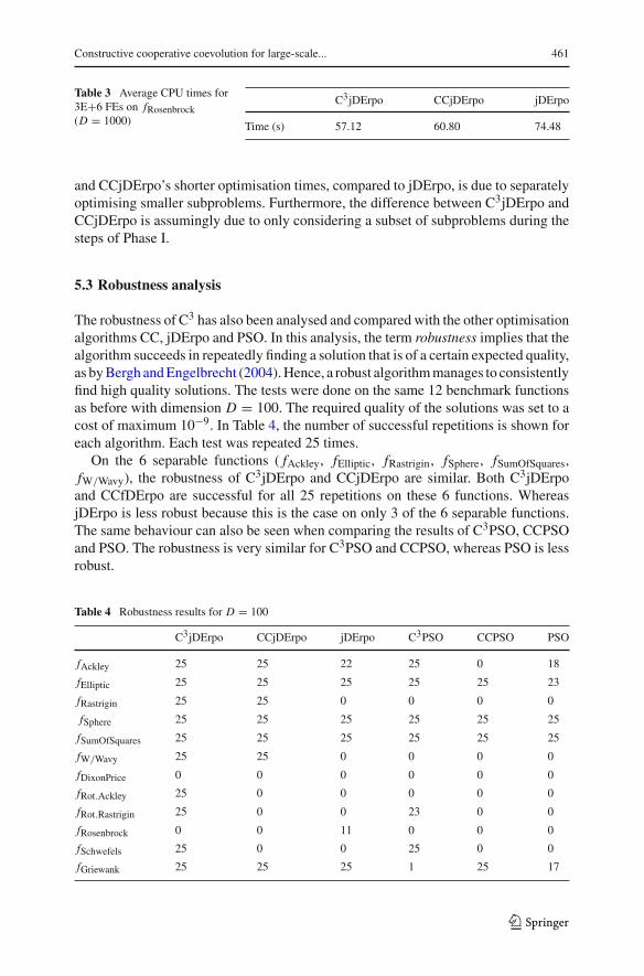
5.3 Robustness analysis

The robustness of C3 has also been analysed and compared with the other optimisationalgorithms CC, jDErpo and PSO. In this analysis, the term robustness implies that thealgorithm succeeds in repeatedly finding a solution that is of a certain expected quality,as byBergh andEngelbrecht (2004).Hence, a robust algorithmmanages to consistentlyfind high quality solutions. The tests were done on the same 12 benchmark functionsas before with dimension D = 100. The required quality of the solutions was set to acost of maximum 10−9. In Table 4, the number of successful repetitions is shown foreach algorithm. Each test was repeated 25 times.

On the 6 separable functions ( fAckley, fElliptic, fRastrigin, fSphere, fSumOfSquares,fW/Wavy), the robustness of C3jDErpo and CCjDErpo are similar. Both C3jDErpoand CCfDErpo are successful for all 25 repetitions on these 6 functions. WhereasjDErpo is less robust because this is the case on only 3 of the 6 separable functions.The same behaviour can also be seen when comparing the results of C3PSO, CCPSOand PSO. The robustness is very similar for C3PSO and CCPSO, whereas PSO is lessrobust.

Table 4 Robustness results for D = 100

C3jDErpo CCjDErpo jDErpo C3PSO CCPSO PSO

fAckley 25 25 22 25 0 18

fElliptic 25 25 25 25 25 23

fRastrigin 25 25 0 0 0 0

fSphere 25 25 25 25 25 25

fSumOfSquares 25 25 25 25 25 25

fW/Wavy 25 25 0 0 0 0

fDixonPrice 0 0 0 0 0 0

fRot.Ackley 25 0 0 0 0 0

fRot.Rastrigin 25 0 0 23 0 0

fRosenbrock 0 0 11 0 0 0

fSchwefels 25 0 0 25 0 0

fGriewank 25 25 25 1 25 17

123


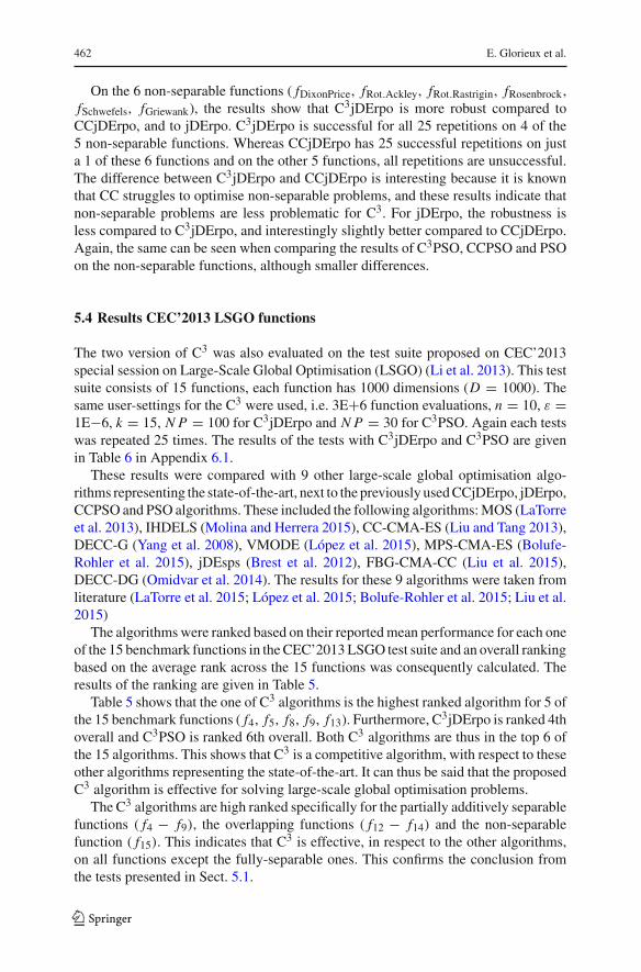
On the 6 non-separable functions ( fDixonPrice, fRot.Ackley, fRot.Rastrigin, fRosenbrock,fSchwefels, fGriewank), the results show that C3jDErpo is more robust compared toCCjDErpo, and to jDErpo. C3jDErpo is successful for all 25 repetitions on 4 of the5 non-separable functions. Whereas CCjDErpo has 25 successful repetitions on justa 1 of these 6 functions and on the other 5 functions, all repetitions are unsuccessful.The difference between C3jDErpo and CCjDErpo is interesting because it is knownthat CC struggles to optimise non-separable problems, and these results indicate thatnon-separable problems are less problematic for C3. For jDErpo, the robustness isless compared to C3jDErpo, and interestingly slightly better compared to CCjDErpo.Again, the same can be seen when comparing the results of C3PSO, CCPSO and PSOon the non-separable functions, although smaller differences.

5.4 Results CEC’2013 LSGO functions

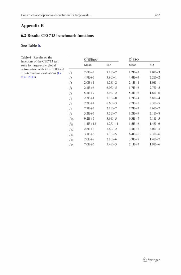
The two version of C3 was also evaluated on the test suite proposed on CEC’2013special session on Large-Scale Global Optimisation (LSGO) (Li et al. 2013). This testsuite consists of 15 functions, each function has 1000 dimensions (D = 1000). Thesame user-settings for the C3 were used, i.e. 3E+6 function evaluations, n = 10, ε =1E−6, k = 15, N P = 100 for C3jDErpo and N P = 30 for C3PSO. Again each testswas repeated 25 times. The results of the tests with C3jDErpo and C3PSO are givenin Table 6 in Appendix 6.1.

These results were compared with 9 other large-scale global optimisation algo-rithms representing the state-of-the-art, next to the previously usedCCjDErpo, jDErpo,CCPSO and PSO algorithms. These included the following algorithms:MOS (LaTorreet al. 2013), IHDELS (Molina and Herrera 2015), CC-CMA-ES (Liu and Tang 2013),DECC-G (Yang et al. 2008), VMODE (López et al. 2015), MPS-CMA-ES (Bolufe-Rohler et al. 2015), jDEsps (Brest et al. 2012), FBG-CMA-CC (Liu et al. 2015),DECC-DG (Omidvar et al. 2014). The results for these 9 algorithms were taken fromliterature (LaTorre et al. 2015; López et al. 2015; Bolufe-Rohler et al. 2015; Liu et al.2015)

The algorithmswere ranked based on their reportedmean performance for each oneof the 15 benchmark functions in theCEC’2013LSGO test suite and an overall rankingbased on the average rank across the 15 functions was consequently calculated. Theresults of the ranking are given in Table 5.

Table 5 shows that the one of C3 algorithms is the highest ranked algorithm for 5 ofthe 15 benchmark functions ( f4, f5, f8, f9, f13). Furthermore, C3jDErpo is ranked 4thoverall and C3PSO is ranked 6th overall. Both C3 algorithms are thus in the top 6 ofthe 15 algorithms. This shows that C3 is a competitive algorithm, with respect to theseother algorithms representing the state-of-the-art. It can thus be said that the proposedC3 algorithm is effective for solving large-scale global optimisation problems.

The C3 algorithms are high ranked specifically for the partially additively separablefunctions ( f4 − f9), the overlapping functions ( f12 − f14) and the non-separablefunction ( f15). This indicates that C3 is effective, in respect to the other algorithms,on all functions except the fully-separable ones. This confirms the conclusion fromthe tests presented in Sect. 5.1.

123


Table5

Algorith

mrank

ingon

the15

benchm

arkfunctio

nsof

theCEC’201

3testsuite

forlarge-scaleglob

alop

timisationwith

D=

1000

(Lietal.2013

)

f 1f 2

f 3f 4

f 5f 6

f 7f 8

f 9f 10

f 11

f 12

f 13

f 14

f 15

Overall

C3jDErpo

1010

102

12

21

112

127

12

54

C3PS

O12

914

16

45

211

142

104

47

6

CCjDErpo

42

1113

1114

1313

1413

138

1313

1313

CCPS

O8

813

1410

1514

1415

1514

914

1415

14

jDErpo

1515

1215

1212

1515

139

1515

1515

1415

PSO

1413

156

913

68

1210

813

77

812

MOS

14

33

78

15

73

51

23

11

IHDELS

26

94

86

34

911

42

31

23

CC-C

MA-ES

97

17

1511

710

65

66

88

98

DECC-G

65

410

135

1111

87

115

1211

1110

VMODE

1112

69

149

89

106

711

65

69

MPS

-CMA-ES

511

75

23

47

34

34

56

32

jDEsps

31

28

41

126

42

103

1110

105

FBG-C

MA-C

C7

35

123

109

32

81

1210

1212

7

DECC-D

G13

148

115

710

125

19

149

94

11

123


6 Conclusions and future work

The Constructive Cooperative Coevolutionary (C3) algorithm for global optimisa-tion of bound-constrained large-scale global optimisation problems is presented inthis paper. C3 includes a novel constructive heuristic combined with the CooperativeCoevolutionary (CC) algorithm in a multi-start architecture. For each restart, a newgood initial solution is created by the constructive heuristic. The region in the searchspace around the constructed solution is then explored by using it as initial solutionfor CC. The constructive heuristic ensures that a different solution is constructed foreach restart. Thereby, it drives CC to search specific regions of the search space.

C3 was compared with state-of-the-art algorithms on a set of large-scale benchmarkfunctions with up to 1000 dimensions, and on the test suite of CEC’2013 competi-tion on large-scale global optimisation (Li et al. 2013). For the latter, 15 algorithms(including two versions of C3) were compared on the 15 benchmark functions of theCEC’2013 test suite. The latter shows that a C3 algorithm is highest ranked for 5 ofthe 15 benchmark functions, outperforming the top algorithms from the most recentCEC’2015 competition on large-scale global optimisation.

Based on the overall ranking across all benchmark function, the two proposed C3

algorithms are in the top 6 out of 15 algorithms (i.e. C3jDErpo is 4th and C3PSO is6th). The results also showed that C3 outperforms the other algorithms on the partiallyseparable functions and the overlapping functions. Results also showed that there isno extra computational cost with C3. It can thus be concluded that C3 is a competitiveeffective algorithm for large-scale global optimisation.

It was demonstrated that C3 can be embedded with different population-basedoptimisation algorithms for the subproblem optimisation. Results showed that theembedded algorithm can significantly influence C3’s performance. Hence, it is impor-tant to select an optimisation algorithm that is well-suited for the specific subproblemsat hand.

Future work with C3 should investigate whether it is rewarding to use automaticdecomposition strategies (i.e. parameter grouping), instead of a static decomposition asused in this work. An adaptive or dynamic decomposition strategywould be preferablein order to adjust the decomposition during the search. This could further improve theperformance and abilities of the C3 algorithm.

Open Access This article is distributed under the terms of the Creative Commons Attribution 4.0 Interna-tional License (http://creativecommons.org/licenses/by/4.0/), which permits unrestricted use, distribution,and reproduction in any medium, provided you give appropriate credit to the original author(s) and thesource, provide a link to the Creative Commons license, and indicate if changes were made.

123

http://creativecommons.org/licenses/by/4.0/


Appendix A

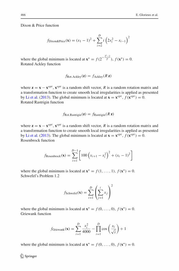
6.1 Benchmark functions

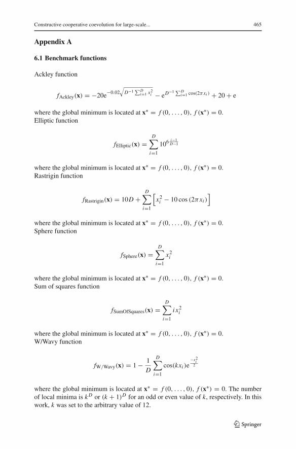
Ackley function

fAckley(x) = −20e−0.02√

D−1∑D

i=1 x2i − eD

−1 ∑Di=1 cos(2πxi ) + 20 + e

where the global minimum is located at x∗ = f (0, . . . , 0), f (x∗) = 0.Elliptic function

fElliptic(x) =D

∑

i=1

106i−1D−1

where the global minimum is located at x∗ = f (0, . . . , 0), f (x∗) = 0.Rastrigin function

fRastrigin(x) = 10D +D

∑

i=1

[

x2i − 10 cos (2πxi )]

where the global minimum is located at x∗ = f (0, . . . , 0), f (x∗) = 0.Sphere function

fSphere(x) =D

∑

i=1

x2i

where the global minimum is located at x∗ = f (0, . . . , 0), f (x∗) = 0.Sum of squares function

fSumOfSquares(x) =D

∑

i=1

i x2i

where the global minimum is located at x∗ = f (0, . . . , 0), f (x∗) = 0.W/Wavy function

fW/Wavy(x) = 1 − 1

D

D∑

i=1

cos(kxi )e−x2i2

where the global minimum is located at x∗ = f (0, . . . , 0), f (x∗) = 0. The numberof local minima is kD or (k + 1)D for an odd or even value of k, respectively. In thiswork, k was set to the arbitrary value of 12.

123


Dixon & Price function

fDixon&Price(x) = (x1 − 1)2 +D

∑

i=2

i(

2x2i − xi−1

)2

where the global minimum is located at x∗ = f (2− 2i−22i ), f (x∗) = 0.

Rotated Ackley function

fRot.Ackley(z) = fAckley(R z)

where z = x − xopt , xopt is a random shift vector, R is a random rotation matrix anda transformation function to create smooth local irregularities is applied as presentedby Li et al. (2013). The global minimum is located at x = xopt , f (xopt ) = 0.Rotated Rastrigin function

fRot.Rastrigin(z) = fRastrigin(R z)

where z = x − xopt , xopt is a random shift vector, R is a random rotation matrix anda transformation function to create smooth local irregularities is applied as presentedby Li et al. (2013). The global minimum is located at x = xopt , f (xopt ) = 0.Rosenbrock function

fRosenbrock(x) =D−1∑

i=1

[

100(

xi+1 − x2i

)2 + (xi − 1)2]

where the global minimum is located at x∗ = f (1, . . . , 1), f (x∗) = 0.Schwefel’s Problem 1.2

fSchwefel(x) =D

∑

i=1

⎛

⎝

i∑

j=1

x j

⎞

⎠

2

where the global minimum is located at x∗ = f (0, . . . , 0), f (x∗) = 0.Griewank function

fGriewank(x) =D

∑

i=1

x2i4000

−D

∏

i=1

cos

(xi√i

)

+ 1

where the global minimum is located at x∗ = f (0, . . . , 0), f (x∗) = 0.

123


Appendix B

6.2 Results CEC’13 benchmark functions

See Table 6.

Table 6 Results on thefunctions of the CEC’13 testsuite for large-scale globaloptimisation with D = 1000 and3E+6 function evaluations (Liet al. 2013)

C3jDErpo C3PSO

Mean SD Mean SD

f1 2.6E−7 7.1E−7 1.2E+3 2.0E+3

f2 4.9E+3 3.9E+1 4.4E+3 2.2E+2

f3 2.0E+1 1.2E−2 2.1E+1 1.0E−1

f4 2.1E+6 6.0E+5 1.7E+6 7.7E+5

f5 5.2E+2 3.9E+2 5.3E+6 1.6E+6

f6 2.3E+1 5.3E+0 1.7E+4 5.8E+4

f7 2.2E+4 6.6E+3 2.7E+5 8.3E+5

f8 7.7E+7 2.1E+7 7.7E+7 3.6E+7

f9 3.2E+7 3.5E+7 1.2E+9 2.1E+8

f10 9.2E+7 3.9E+5 9.3E+7 7.1E+5

f11 1.4E+12 1.2E+11 1.5E+6 1.4E+6

f12 2.6E+3 2.6E+2 3.3E+3 3.0E+3

f13 3.1E+6 7.3E+5 6.4E+6 2.3E+6

f14 2.0E+7 2.8E+6 3.3E+7 1.4E+7

f15 7.0E+6 5.4E+5 2.1E+7 1.9E+6

123


References

Ali, M.M., Khompatraporn, C., Zabinsky, Z.B.: A numerical evaluation of several stochastic algorithms onselected continuous global optimization test problems. J. Glob. Optim. 31(4), 635–672 (2005)

Araújo, T.M.U.D., Andrade, L.M.M.S., Magno, C., Cabral, L.D.A.F., Nascimento, R.Q.D., Meneses, C.N.:DC-GRASP: directing the search on continuous-GRASP. J. Heuristics 22(4), 365–382 (2016)

Bolufe-Rohler, A., Fiol-Gonzalez, S., Chen, S.: A minimum population search hybrid for large scale globaloptimization. In: Evolutionary Computation (CEC), 2015 IEEE Congress on, IEEE, pp. 1958–1965(2015)

Brest, J., Boskovic, B., Zamuda, A., Fister, I., Maucec, M.: Self-adaptive differential evolution algorithmwith a small and varying population size. In: 2012 IEEE Congress on Evolutionary Computation(CEC), pp. 1–8 (2012)

Brest, J., Zamuda, A., Fister, I., Boskovic, B.: Some improvements of the self-adaptive jDE algorithm. In:IEEE Symposium on Differential Evolution (SDE), pp. 1–8 (2014)

Feo, T.A., Resende,M.G.C.: Greedy randomized adaptive search procedures. J. Glob. Optim. 6(2), 109–133(1995)

García, S., Molina, D., Lozano, M., Herrera, F.: A study on the use of non-parametric tests for analyzing theevolutionary algorithms’ behaviour: a case study on the CEC’2005 special session on real parameteroptimization. J. Heuristics 15(6), 617–644 (2009)

Glorieux, E., Danielsson, F., Svensson, B., Lennartson, B.: Optimisation of interacting production sta-tions using a constructive cooperative coevolutionary approach. In: IEEE International Conference onAutomation Science and Engineering (CASE), pp. 322–327 (2014)

Glorieux, E., Danielsson, F., Svensson, B., Lennartson, B.: Constructive cooperative coevolutionary opti-misation for interacting production stations. Int. J. Adv. Manuf. Technol. 80(1–4), 673–688 (2015)

Grendreau,M., Potvin, J.Y. (eds.): Handbook ofMetaheuristics. International Series in Operations Research& Management Science, vol. 146, 2nd edn. Springer, USA (2010)

Hirsch, M.J., Meneses, C.N., Pardalos, P.M., Resende, M.G.C.: Global optimization by continuous grasp.Optim. Lett. 1(201–212), 2 (2007)

Hirsch, M., Pardalos, P., Resende, M.: Speeding up continuous GRASP. Eur. J. Oper. Res. 205(3), 507–521(2010)

Jamil, M., Yang, X.: A literature survey of benchmark functions for global optimisation problems. Int. J.Math. Model. Numer. Optim. 4(2), 150–194 (2013)

LaTorre, A., Muelas, S., Pena, JM.: Large scale global optimization: experimental results with mos-basedhybrid algorithms. In: Evolutionary Computation (CEC), 2013 IEEE Congress on, IEEE, pp. 2742–2749 (2013)

LaTorre, A., Muelas, S., Peña, J.M.: A comprehensive comparison of large scale global optimizers. Inf. Sci.316, 517–549 (2015)

Li, X., Yao,X.: Tackling high dimensional nonseparable optimization problems by cooperatively coevolvingparticle swarms. In: IEEE Congress on Evolutionary Computation, 2009. CEC ’09, pp. 1546–1553(2009)

Li, X., Yao, X.: Cooperatively coevolving particle swarms for large scale optimization. IEEE Trans. Evol.Comput. 16(2), 210–224 (2012)

Li, X., Tang, K., Omidvar, MN., Yang, Z., Qin, K.: Benchmark functions for the CEC’2013 special sessionand competition on large-scale global optimization. Technical report, evolutionary computation andmachine learning group, RMIT University, Australia (2013)

Liu, H., Guan, S., Liu, F., Wang, Y.: Cooperative co-evolution with formula based grouping and CMA forlarge scale optimization. In: 2015 11th International Conference on Computational Intelligence andSecurity (CIS), pp. 282–285 (2015)

Liu, J., Tang, K.: Scaling up covariance matrix adaptation evolution strategy using cooperative coevolution.In: Yin, H., Tang, K., Gao, Y., Klawonn, F., Lee, M., Weise, T., Li, B., Yao, X. (eds.) Intelligent DataEngineering and Automated Learning—IDEAL 2013. Lecture Notes in Computer Science, vol. 8206,pp. 350–357. Springer, Berlin (2013)

López, E.D., Puris, A., Bello, R.R.: VMODE: a hybrid metaheuristic for the solution of large scale opti-mization problems. Revista Investigacion Operacional 36(3), 232–239 (2015)

Lozano,M.,Molina,D., Herrera, F.: Editorial scalability of evolutionary algorithms and othermetaheuristicsfor large-scale continuous optimization problems. Soft Comput. 15(11), 2085–2087 (2011)

123


Martí, R., Moreno-Vega, J.M., Duarte, A.: Advanced multi-start methods. In: Gendreau, M., Potvin, J.Y.(eds.) Handbook of Metaheuristics. International Series in Operations Research & Management Sci-ence, vol. 146, pp. 265–281. Springer, New York (2010)

Molina, D., Herrera, F.: Iterative hybridization of DE with local search for the CEC’2015 special sessionon large scale global optimization. In: 2015 IEEE Congress on Evolutionary Computation (CEC), pp.1974–1978 (2015)

Nickabadi, A., Ebadzadeh, M.M., Safabakhsh, R.: A novel particle swarm optimization algorithm withadaptive inertia weight. Appl. Soft Comput. 11(4), 3658–3670 (2011)

Omidvar, M., Li, X., Yang, Z., Yao, X.: Cooperative co-evolution for large scale optimization through morefrequent random grouping. In: IEEE Congress on Evolutionary Computation, 2010. (CEC’10), pp.1–8 (2010)

Omidvar, M., Li, X., Mei, Y., Yao, X.: Cooperative co-evolution with differential grouping for large scaleoptimization. IEEE Trans. Evol. Comput. 18(3), 378–393 (2014)

Potter, M.A., De Jong, K.A.: A cooperative coevolutionary approach to function optimization. In: Davidor,Y., Schwefel, H.P., Männer, R. (eds.) Parallel Problem Solving fromNature—PPSN III. Lecture Notesin Computer Science, vol. 866, pp. 249–257. Springer, Berlin (1994)

Potter, M.A., De Jong, K.A.: Cooperative coevolution: an architecture for evolving coadapted subcompo-nents. Evol. Comput. 8(1), 1–29 (2000)

Ray, T., Yao, X.: A cooperative coevolutionary algorithm with correlation based adaptive variable parti-tioning. In: IEEE Congress on Evolutionary Computation, 2009. CEC ’09, pp. 983–989 (2009)

Schutte, J.F., Groenwold, A.A.: A study of global optimization using particle swarms. J. Glob. Optim. 31(1),93–108 (2005)

Shi, Y., Teng, H., Li, Z.: Cooperative co-evolutionary differential evolution for function optimization. In:Proc. of International Conference on Natural Computation, pp. 1080–1088 (2005)

Van den Bergh, F., Engelbrecht, A.: A cooperative approach to particle swarm optimization. IEEE Trans.Evol. Comput. 8(3), 225–239 (2004)

Wiegand, RP., Liles, WC., Jong, KAD.: An empirical analysis of collaboration methods in cooperativecoevolutionary algorithms. In: Proc. from the Genetic and Evolutionary Computation Conference,Morgan Kaufmann, pp. 1235–1242 (2001)

Yang, Z., Tang, K., Yao, X.: Large scale evolutionary optimization using cooperative coevolution. Inf. Sci.178(15), 2985–2999 (2008)

Zamuda, A., Brest, J., Boskovic, B., Zumer, V.: Large scale global optimization using differential evolutionwith self-adaptation and cooperative co-evolution. In: Proc. Congr. Evolutionary Computation (CEC08), pp. 3718–3725 (2008)

123

Documents

Constructive cooperative coevolution for large-scale ...publications.lib.chalmers.se/records/fulltext/253271/local_253271.pdfConstructive cooperative coevolution for large-scale