Embed Size (px)
Citation preview
CONSTRUCTION-RELATED IMPACTS OF THE
TRANS-ALASKA PIPELINE SYSTEM ON TERRESTRIAL WILDLIFE HABITATS
AUGUST1979
us. ... l;.r \ - ..... IHt. ~·
"i.- t~:'ll Ala~ka .:..;.oloqicc .>arv::- • A'lchorcrge, Alw.;';tT
doint State I Federal Fish & Wildlife Advisory Team
\
r t • ' [
t
CONSTRUCTION-RELATED IMPACTS OF THE TRANS-ALASKA PIPELINE SYSTEM
ON TERRESTRIAL WILDLIFE HABITATS
By: W. Lewis Pamplin, Jr.
August, 1979
Special Report Number 24
JOINT STATE/FEDERAL FISH AND.WILDLIFE ADVISORY TEAM
SPONSORED BY THE
U.S. Department of the Interior, Alaska Pipeline Office
State of Alaska, Pipeline Coordinator's Office
U.S. Fish and Wildlife Service Alaska Department of Fish and Game
Bureau of Land Management National Marine Fisheries Service Alyeska Pipeline Service Company
Permission to reproduce any of the information contained herein is withheld pending approval of the author.
CONTENTS
PREFACE and ACKNOWLEDGMENTS ••••••••••••• • • • • • • ••••• • • • • • • • • • • • Page
i
.ABSTRACT •••••••••••••••••••••••••••••• • • • • • • • • • • • • • • • • • • • • • • • • ii
INTRODUCTION • • • • • • • • • • • • • • • • • • • • • • • • • • • • • • • • • • • • • • • • • • • • • • • • • • 1
STUDY AREA
PROCEDURES .................................................... Quantitative Phase
Qualitative Phase ......................................... FINDINGS .......................................................
Habitat Typing
4
7
21
26
29
29
Habitat Quality . . . . . . . . . . . . . . . . . . . . . . . . . . . . . . . . . . . . . . . . . . . 32
Construction-Related Impacts ....................... Impacts
Impacts
by
by
Land Ownership
Construction Section ••
Impacts by Construction Activity
DISCUSSION .••••••..•••••.••••••.•••••..•••. ·'· ••••••..••••••.•••
RECO:MMENDATIONS
SUMMARY ........................................................ REFERENCES ...................................................... APPENDICES .....................................................
Appendix I: Glossary ............................. . . . . . . Appendix II: Pipeline Construction-Related Impacts ...... Appendix III: Wildlife Evaluation Elements ....... Appendix IV: Rating Entries and Contingency Tables ...... Appendix V: Plates (13 - 34) ...........................
35
35
42
42
52
58
61
63
70
70
73
91
96
121
PREFACE and ACKOWLEDGEMENTS
In 1974 the Joint State/Federal Fish and Wildlife Advisory Team (JFWAT) was organized to monitor the construction of the Trans-Alaska Pipeline System (TAPS). JFWAT was disbanded in December, 1977 after TAPS construction and major restoration activities were completed. During this period (1975 to 1977), JFWAT conducted a terrestrial habitat evaluation to determine the impacts of TAPS construction on terrestrial wildlife habitats. Most of the basic data for this evaluation was obtained prior to JFWAT's disbandment. Final data compilation and data analysis were completed in 1978 after the author returned to regular duties with the U.S. Fish and Wildlife Service (FWS).
This report does not include copies of the habitat-type maps developed during the evaluation. The enlarged pre-construction photographs used to map habitat types are currently located in the FWS Area Office in Anchorage. The author hopes that in the near future funds can be obtained to permit these data to be transferred to topographic base maps and published in a format suitable for office and field work involving vegetation analyses along the TAPS.
The plates (photographs) used in this report are organized into two main groups: (1) the twelve habitat types and (2) examples of pipeline constructionrelated impacts. Descriptions of key terms used in this report are contained in Appendix I.
I would like to thank Jim Hemming, Hank Hosking, Al Carson, and Carl Yanagawa for their support and encouragement throughout the evaluation. The efforts of the JFWAT biologists who participated in the collection of collateral field data and in the development of the qualitative phase of the evaluation are appreciated.
I am indebted to Erik Westman, the principal photo interpreter and main biological assistant, for his dedication to this project and his many outstanding accomplishments. Erik's contributions were a major factor in the successful completion of this evaluation.
I would like to thank SuzAnne Miller for her expert assistance in statistical analysis of the qualitative data. The following persons took time from busy schedules to review complete drafts of this report and offered comments which I greatly appreciate: Dirk Derksen, Jim Glaspell, Nancy Hemming, Hank Hosking, Norval Netsch, and Al Ott. I accept, however, full responsibility for the final statements and conclusions. I am grateful to Paula Wade and Joyce Hursh for typing and editing this report and to Mel Monson for allowing me the time to finish it.
Funds for printing this report were provided by the FWS, Area Office Ecological Services in Anchorage. Copies of this report may be obtained by contacting the following offices:
(1) Area Office Ecological Services u.s. Fish and Wildlife Service 1011 E. Tudor Road Anchorage, Alaska 99503 (907) 276-3800, ext. 469
i
(2) Pipeline Surveillance Office Alaska Department of Fish and Game 520 E. 4th Avenue Anchorage, Alaska 99501 (907) 276-8410
ABSTRACT
The Joint State/Federal Fish and Wildlife Advisory Team (JFWAT) conducted a terrestrial habitat evaluation of the 800-mile Trans-Alaska Pipeline System (TAPS). The purposes of this project were to identify and evaluate wildlife habitats along the TAPS and determine the quantitative and qualitative impacts of TAPS construction on these habitats. Using a classification system consisting of twelve habitat types, the study area (about 2150 square miles) was cover typed on pre-construction aerial imagery. Post-construction imagery of the same scale was used to determine the surface area impacts. Approximately 31,403 acres of terrestrial wildlife habitat were altered or destroyed by construction activities as of July, 1976.
About 66.7% of the impacts were on federal land while 28.9% and 4.4% were on state and private lands, respectively. Construction~
Section 6 had the greatest overall impact (10,900 acres) and Section 3 had the least (2,946 acres). Nearly one-half of the impacts were on high (wetlands and wet-meadow tundra) and high-medium (spruce-deciduous woodland, shrub thicket, and riparian willow) quality wildlife habitats.
Material sites caused the most habitat alteration (11,828 acres) of any construction activity. The work pad, Yukon River to Prudhoe Bay Haul Road, and access roads produced habitat losses of 10,610 acres, 3,751 acres, and 1,196 acres, respectively, and were the most detrimental construction activities to high quality wildlife habitats.
Recommendations for minimizing adverse impacts to wildlife habitats are made for the operational phase of TAPS and future projects including oil and gas pipelines, roads, water-related projects, and mining. Interagency/inter-disciplinary teams must be used to evaluate potential impacts of future developments on wildlife habitats if unnecessary and avoidable impacts are to be eliminated or minimized. Habitat evaluations should be conducted during the planning stage of major projects so that impacts by habitat type can be identified and the least damaging alternatives selected. Mitigative measures must be incorporated into project designs when unavoidable adverse impacts occur to wildlife habitats.
ii

INTRODUCTION
Background
In 1968 oil was discovered at Prudhoe Bay on Alaska's Arctic Coastal Plain. The following year several oil companies applied for state permits and a Bureau of Land Management (BLM) right-of-way permit to construct a pipeline across state and federal lands in Alaska. The federal government was temporarily stopped from issuing the permit due to legal suits filed by national environmental organizations.
Litigation evolved around the requirements of the National Environmental Policy Act of 1969 and the Mineral Leasing Act of 1920. A final environmental impact statement was issued by the Secretary of Interior in March, 1972 (U.S. Dept. Int. 1972). In November, 1973, Congress passed Public Law 93-153 (TransAlaska Pipeline Authorization Act) which, among other things, amended the Mineral Leasing Act so that a BLM permit could then be issued for pipeline construction which required an increased right-of-way width.
In early 1974, a consortium of seven major oil companines (Amerada Hess Corp., ARCO Pipeline Co., Exxon Pipeline Co., Mobil Alaska Pipeline Co., Phillips Petroleum Co., Sohio Pipeline Co., and Union Alaska Pipeline Co.) signed agreements and grants of right-of-way with both the United States of America (U.S. Dept. Int. 1974) and the State of Alaska. With the major legal requirements resolved, the aforementioned companies designated Alyeska Pipeline Service Company (APSC) to function as the Permittee for construction, operation, maintenance, and termination of the Trans-Alaska Pipeline System (TAPS). APSC thus became the oil industry's agent responsible for ensuring that the provisions (e.g. environmental and technical stipulations) contained in the federal and state agreements and grants of right-of-way would be followed. Certain other requirements also were mandated. For example, the Permittee through its Quality Assurance Program was to ensure that impacts to fish and wildlife resources were minimized during the construction, operation, maintenance, and termination of the TAPS (U.S. Dept. Int. 1974).
In Section 13 of the Agreement and Grant of Right-of-Way for Trans-Alaska Pipeline between the federal government and the Permittees (U.S. Dept. Int. 1974), a requirement was set forth such that the Permittees:
"(2) shall rehabilitate (including but not limited to, revegetation, restocking fish or other wildlife populations and re-establishing their habitats), to the written satisfaction of the Authorized Officer, any natural resource that shall be seriously damaged or destroyed, if the immediate cause of the damage or destruction arises out of, is connected with, or results from, the construction, operation, maintenance or termination of all or any part of the Pipeline System".
The above requirements may appear stringent; however, it should be remembered that the TAPS project was controversial and unprecedented in Alaska's arctic and subarctic environments. There was, and continues to be, a great potential for serious and long-term environmental damage. Prior to TAPS, the
1
concepts of mitigation (i.e. lessening impacts) and compensation (i.e. replacing or reestablishing) of altered and destroyed fish and wildlife habitats had been established nationwide. These principles have been applied to federally funded and permitted water-related development projects. In the past decade, the American public has demanded that fish and wildlife values receive adequate protection when threatened by major development projects.
The terms and conditions of the state and federal right-of-way agreements (e.g. environmental and technical stipulations) provided the mechanisms to protect public fish and wildlife resources. Enforcement of the stipulations was the primary vehicle for ensuring that unnecessary and avoidable adverse impacts were minimized during construction. However, regardless of the degree of environmental stipulation compliance by APSC, it was inevitable that unavoidable and, in many instances, irreparable damages would occur to fish and wildlife habitats.
Construction of the TAPS started in the spring of 1974. The Joint State/Federal Fish and Wildlife Advisory Team (JFWAT) was organized during this same time period, under the authority of Section II, Paragraph 6 of the Cooperative Agreement between the United States Department of the Interior and the State of Alaska regarding the proposed transAlaska Pipeline (U.S. Dept. Int. 1974). JFWAT was not fully staffed for field monitoring until late fall 1974. The purpose of JFWAT was to function as a single interagency team of professional biologists who would provide for the protection of fish and wildlife resources by cooperative effort over the length of the pipeline on both state and federal lands. Biologists from the Alaska Department of Fish and Game (ADF&G), BLM, National Marine Fisheries Service (NMFS), and U.S. Fish and Wildlife Service (FWS) participated in this joint effort.
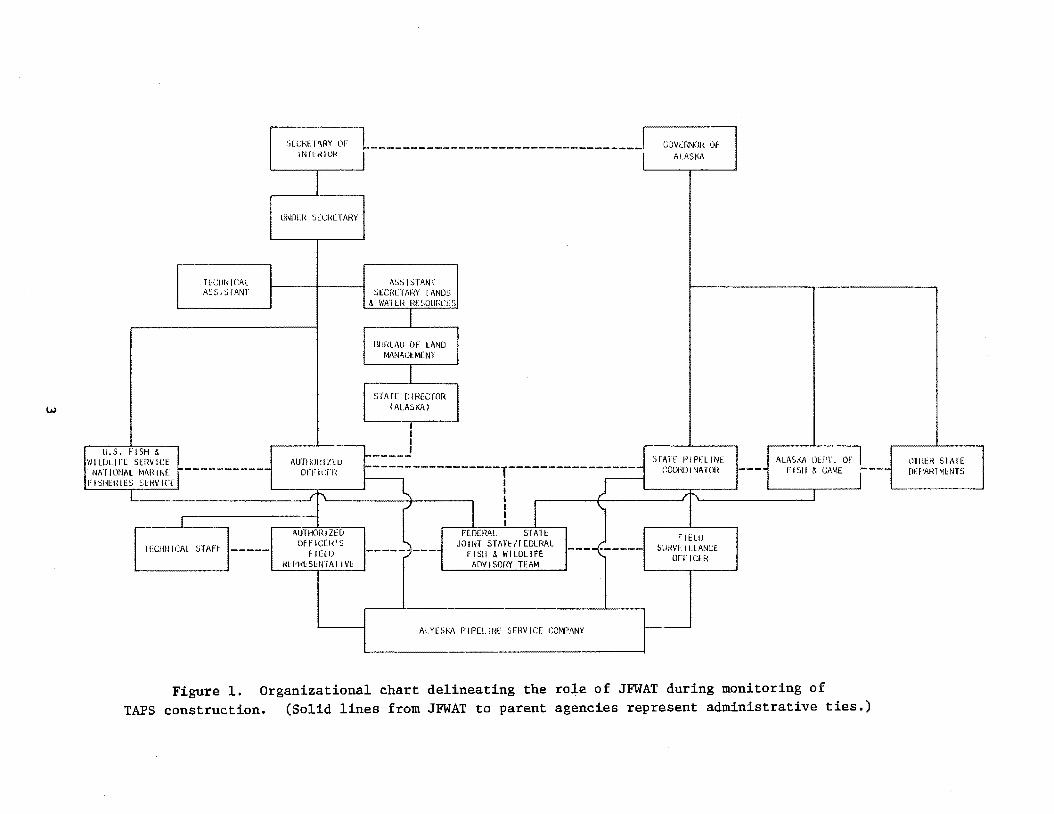
JFWAT functioned as a line component of both the federal government's Alaska Pipeline Office (APO) and the State Pipeline Coordinator's Office (SPCO) (Figure 1) and coordinated many of the pipeline-related statutory and regulatory responsibilities of the cooperating resource agencies. The primary objective of JFWAT was to ensure that the construction and future operation of the TAPS caused only minimal adverse impacts, both short and long-term, to fish and wildlife populations and their habitats.
APO and SPCO were responsible for enforcing the right-of-way agreements and stipulations on federal and state lands. JFWAT recommendations and field advices were given to the appropriate offices and field representatives of APO and SPCO and pertained to the following items:
(1) design review of technical documents, change orders, contingency plans, and permit applications submitted by APSC;
(2) the Permittee's compliance with environmental stipulations during the construction phase of the project; and
2
U.S. FISH & WI UJU F£ SEHV ICE
TI:CIINICAL ASSI:JfANT
NAT IOI'JAL ~IAHINE -----------
OitCH£: 11\RY 01' ·-1~,...----------------------------------'~· I!WRIOI\
~--+-----
1\UTfiOI<I ZUJ OfF liTH
AS~ I STAN I SlCHLTARY I ANOS
.~ WAHl< 1\f.~,Qllf\CI: :;
I l:lUf\l/IU OF LAND
MIINf,G~.MENT
I STAlE DIHECfOR I
(ALASKA) .J I I I
1-----J -----------------r-----------------
GOVERNOH Of ALASKA
~ fATF PI PH INf. I ~OOI{Ill NA TOB
ALASKA DlPT. OF l tlTHER STArE DH'AR1MI::NTS
~ I ) m.r\.1-zE_o _____ I-+-----r:~IERAL l )1\f.--l,----2+----,_---_ -_-_ -'-L---...,
FISHEHIES SlHVICf
I
FISII & CAME
1
----
1 L---------~ '-----------..J
I
OFFICEI<'S JOINT STAH/FEDLHAL FltliJ FICtD -----·--- FISII & WILDLIFE --- ·----- SliHVLILLANC£
RFf'l<lS~tHAliVl ADVISORY TEAM OfFIC~R lFCHNICAL STAH -----
ALYESKA PIPU.INf SERVICE COMPANY
Figure 1. Organizational chart delineating the role of JFWAT during monitoring of TAPS construction. (Solid lines from JFWAT to parent agencies represent administrative ties.)
(3) determination if as-built structures for fish and wildlife protection and utilization were constructed according to approved designs and specifications.
After being directly involved with continuous surveillance of pipeline construction activities for more than a year~ JFWAT recognized the need for an overall documentation of TAPS construction impacts on fish and wildlife habitats. To fulfill this need~ JFWAT conducted two broad evaluations: one concerned with terrestrial wildlife habitats and one with fish stream habitats. This report pertains only to the former evaluation.
Objectives
The objectives of JFWAT's terrestrial habitat evaluation were:
(1) identify and evaluate the major wildlife habitats along the TAPS;
(2) determine quantitative and qualitative impacts of TAPS construction on terrestrial wildlife habitats;
(3) provide baseline information for future evaluations of long-term habitat alterations caused by developments associated with the TAPS;
(4) provide information and recommendations applicable to future construction projects in subarctic and arctic environments.
STUDY AREA
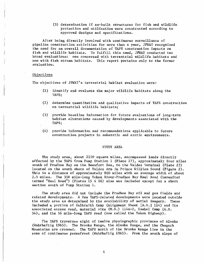
The study area, about 2150 square miles, encompassed lands directly affected by the TAPS from Pump Station 1 (Plate 27), approximately four miles south of Prudhoe Bay on the Beaufort Sea, to the Valdez Terminal (Plate 23) located on the south shore of Valdez Arm in Prince William Sound (Figure 2). This is a distance of approximately 800 miles with an average width of about 2.5 miles. The 358 mile-long Yukon River-Prudhoe Bay Haul Road (hereafter termed "Haul Road") (Plates 15 & 16) also was included except for a short section south of Pump Station 1.
The study area did not include the Prudhoe Bay oil and gas fields and related developments. A few TAPS-related developments were located outside the study area as determined by the availability of aerial imagery. These included a portion of Galbraith Camp (Alignment Sheet [A.S.] 114) and its associated access road, material site (M.S.) 114A-2, Isabel Camp (A.S. 34), and the 56 mile-long TAPS road (now called the Yukon Highway).
The TAPS traverses eight of twelve physiographic provinces of Alaska (Wahrhaftig 1965). The Brooks Range, the Alaska Range, and the Chugach Mountains are crossed. The TAPS north of the Brooks Range lies in the zone of continuous permafrost (Wahrhaftig 1965). From the south slope of
4
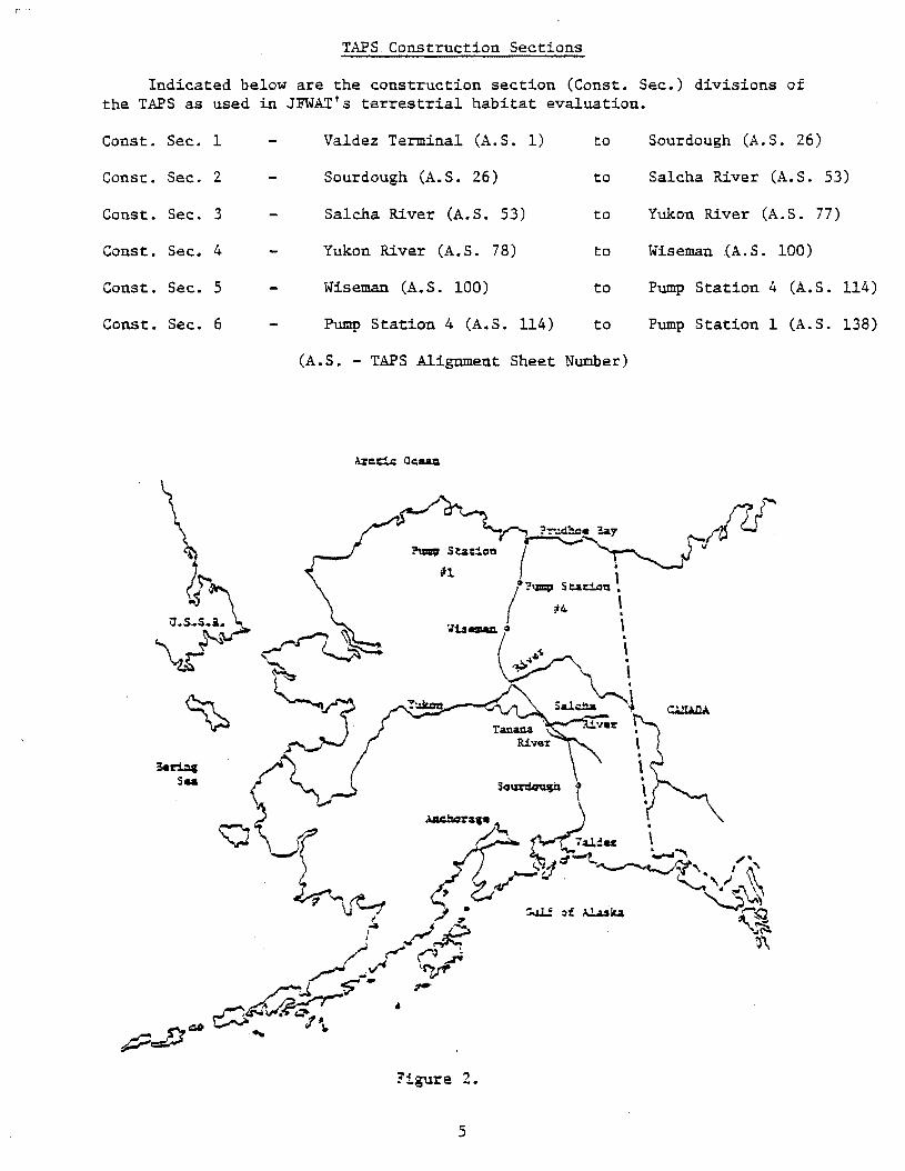
TAPS Construction Sections
Indicated below are the construction section (Const. Sec.) divisions of the TAPS as used in J'FWAT's terrestrial habitat evaluation.
Const. Sec. 1 Valdez Terminal (A. S. 1) to Sourdough (A. S. 26)
Const. Sec. 2 Sourdough (A.S. 26) to Salcha River (A.S. 53)
Const. Sec. 3 Salcha River (A.S. 53) to Yukon River (A.S. 77)
Const. Sec. 4 Yukon River (A.S. 78) to Wiseman (A.S. 100)
Const. Sec. 5 Wiseman (A.S. 100) to Pump Station 4 (A. S. 114)
Const. Sec. 6 Pump Station 4 (A.S. 114) to Pump Station 1 (A. S. 138)
(A.S. - TAPS Alignment Sheet Number)
. \ . \ . l 1
?igure 2.
5
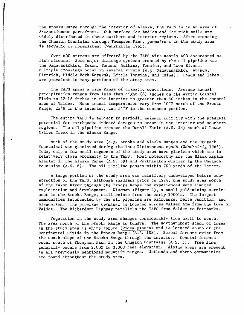
1 the Brooks Range through the interior of Alaska, the TAPS is in an area of discontinuous permafrost. Sub-surface ice bodies and ice-rich soils are widely distributed in these northern and interior regions. After crossing the Chugach Mountains through Thompson Pass, permafrost in the study area is sporadic or nonexistent (Wahrhaftig 1965).
Over 600 streams are affected by the TAPS with nearly 400 documented as fish streams. Some major drainage systems crossed by the oil pipeline are the Sagavanirktok, Yukon, Tanana, Gulkana, Tonsina, and Lowe Rivers. Multiple crossings occur in several rivers (e.g. Sagavanirktok, Atigun, Dietrich, Middle Fork Koyukuk, Little Tonsina, and Tsina). Ponds and lakes are prevalent in many portions of the study area.
The TAPS spans a wide range of climatic conditions. Average annual precipitation ranges from less than eight (8) inches on the Arctic Coastal Plain to 12-16 inches in the interior to greater than 60 inches in the coastal area of Valdez. Mean annual temperatures vary from l0°F north of the Brooks Range, 25°F in the interior, and 34°F in the southern portion.
The entire TAPS is subject to periodic seismic activity with the greatest potential for earthquake-induced damages to occur in the interior and southern regions. The oil pipeline crosses the Denali Fault (A.S. 38) south of Lower Miller Creek in the Alaska Range.
Much of the study area (e.g. Brooks and Alaska Ranges and the Chugach Mountains) was glaciated during the late Pleistocene epoch (Wahrhaftig 1965). Today only a few small segments of the study area have glaciers which are in relatively close proximity to the TAPS. Most noteworthy are the Black Rapids Glacier in the Alaska Range (A.S. 39) and Worthington Glacier in the Chugach Mountains (A.S. 6). The oil pipeline passes within 700 yards of the latter.
A large portion of the study area was relatively undeveloped before construction of the TAPS. Although roadless prior to 1974, the study area north of the Yukon River through the Brooks Range had experienced very limited exploitation and development. Wiseman (Figure 2), a small gold-mining settlement in the Brooks Range, still exists from the early 1900's. The largest communities intersected by the oil pipeline are Fairbanks, Delta Junction, and Glennallen. The pipeline terminal is located across Valdez Arm from the town of Valdez. The Richardson Highway parallels the TAPS from Valdez to Fairbanks.
Vegetation in the study area changes considerably from north to south. The area north of the Brooks Range is tundra. The northernmost stand of trees in the study area is white spruce (Picea glauca) and is located south of the Continental Divide in the Brooks Range (A.S. 108). Boreal forests exist from the south slope of the Brooks Range through the interior. Coastal forests occur south of Thompson Pass in the Chugach Mountains (A.S. 5). Tree line generally occurs from 2,000 to 3,000 feet elevation. Alpine areas are present in all previously mentioned mountain ranges. Wetlands and shrub communities are found throughout the study area.
6
PROCEDURES
General
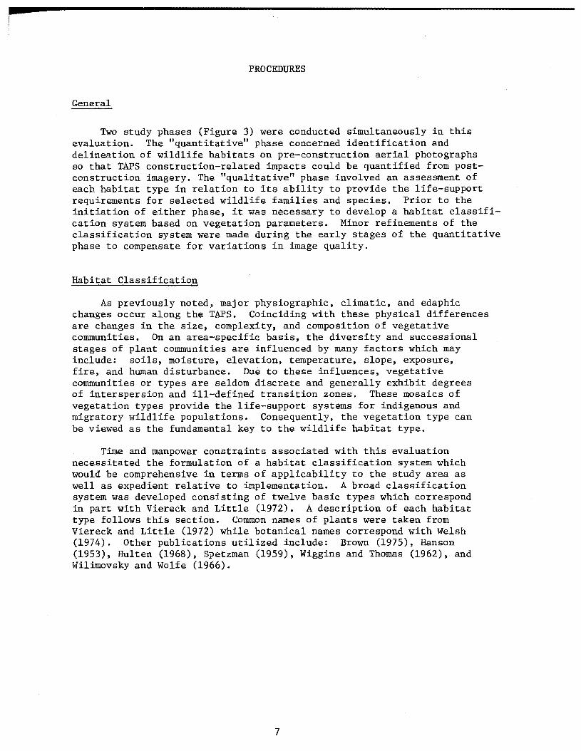
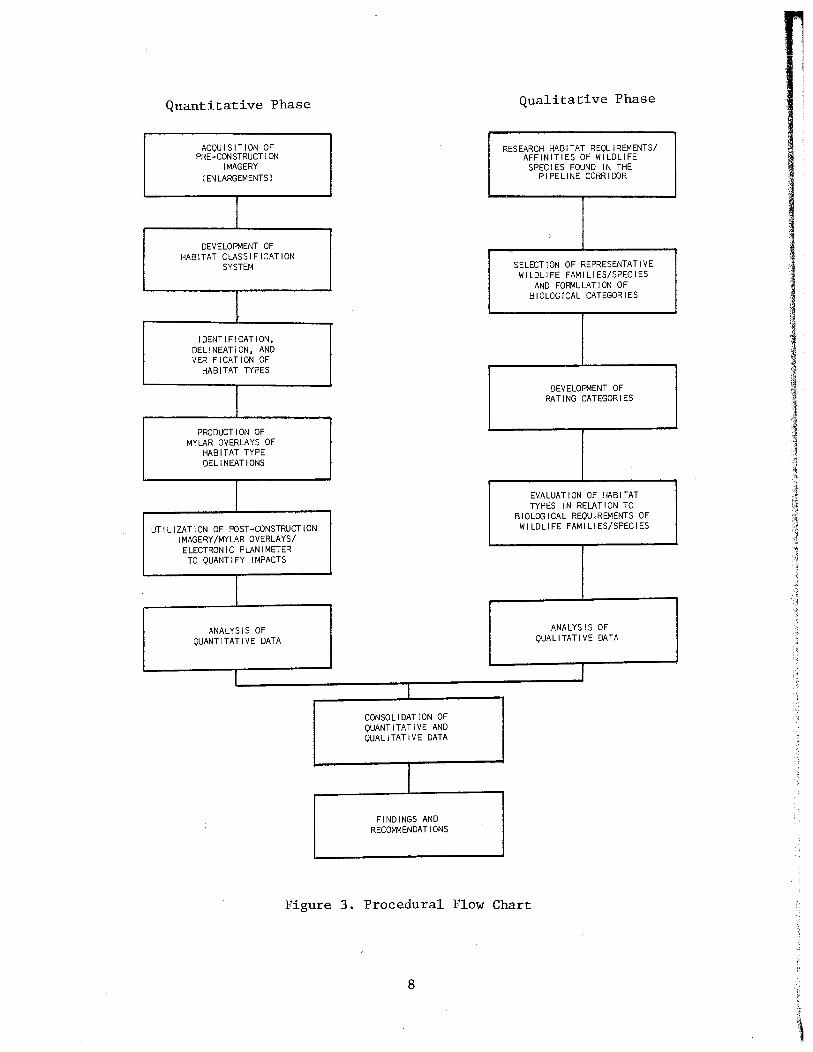
Two study phases (Figure 3) were conducted simultaneously in this evaluation. The "quantitative" phase concerned identification and delineation of wildlife habitats on pre-construction aerial photographs so that TAPS construction-related impacts could be quantified from postconstruction imagery. The "qualitative" phase involved an assessment of each habitat type in relation to its ability to provide the life-support requirements for selected wildlife families and species. Prior to the initiation of either phase, it was necessary to develop a habitat classification system based on vegetation parameters. Minor refinements of the classification system were made during the early stages of the quantitative phase to compensate for variations in image quality.
Habitat Classification
As previously noted, major physiographic, climatic, and edaphic changes occur along the TAPS. Coinciding with these physical differences are changes in the size, complexity, and composition of vegetative communities. On an area-specific basis, the diversity and successional stages of plant communities are influenced by many factors which may include: soils, moisture, elevation, temperature, slope, exposure, fire, and human disturbance. Due to these influences, vegetative communities or types are seldom discrete and generally exhibit degrees of interspersion and ill-defined transition zones. These mosaics of vegetation types provide the life-support systems for indigenous and migratory wildlife populations. Consequently, the vegetation type can be viewed as the fundamental key to the wildlife habitat type.
Time and manpower constraints associated with this evaluation necessitated the formulation of a habitat classification system which would be comprehensive in terms of applicability to the study area as well as expedient relative to implementation. A broad classification system was developed consisting of twelve basic types which correspond in part with Viereck and Little (1972). A description of each habitat type follows this section. Common names of plants were taken from Viereck and Little (1972) while botanical names correspond with Welsh (1974). Other publications utilized include: Brown (1975), Hanson (1953), Hulten (1968), Spetzman (1959), Wiggins and Thomas (1962), and Wilimovsky and Wolfe (1966).
7
Quantitative Phase Qualitative Phase
ACQUISITION OF RESEARCH HABITAT REQUIREMENTS/ PRE-CONSTRUCTION AFFINITIES OF WILDLIFE
IMAGERY SPECIES FOUND IN THE (ENLARGEMENTS) PIPELINE CORRIDOR
I )
DEVELOPMENT OF HABITAT CLASSIFICATION
SYSTEM SELECTION OF REPRESENTATIVE WILDLIFE FAMILIES/SPECIES
AND FORMULATION OF
l BIOLOGICAL CATEGORIES
IDENTIFICATION, DELINEATION, AND VERIFICATION OF
HABITAT TYPES
I DEVELOPMENT OF
RATING CATEGORIES
PRODUCTION OF MYLAR OVERLAYS OF
HABITAT TYPE DELl NEAT IONS
I EVALUATION OF HABITAT TYPES IN RELATION TO
BIOLOGICAL REQUIREMENTS OF UTILIZATION OF POST-CONSTRUCTION WILDLIFE FAMILIES/SPECIES
IMAGERY/MYLAR OVERLAYS/ ELECTRONIC PLANIMETER
TO QUANTIFY IMPACTS
I j ~'
ANALYSIS OF ANALYSIS OF QUANTITATIVE DATA QUALITATIVE DATA
I I
CONSOLIDATION OF QUANTITATIVE AND QUALITATIVE DATA
I FINDINGS AND
RECOMMENDATIONS
Figure 3. Procedural Flow Chart
8
Coastal Forest (01)
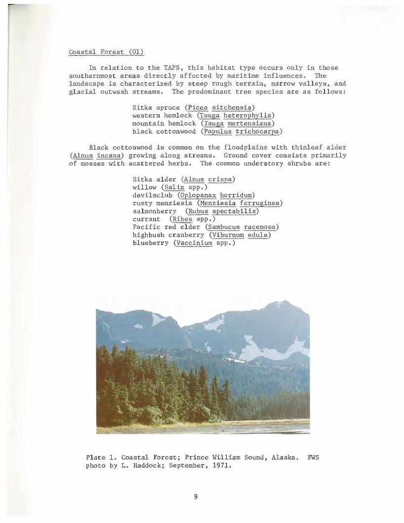
In relation to the TAPS, this habitat type occurs only in those southernmost areas directly affected by maritime influences. The landscape is characterized by steep rough terrain, narrow valleys, and glacial outwash streams. The predominant tree species are as follows:
Sitka spruce (Picea sitchensis) western hemlock (Tsuga heterophylla) mountain hemlock (Tsuga mertensiana) black cottonwood (Populus trichocarpa)
Black cottonwood is common on the floodplains with thinleaf alder (Alnus incana) growing along streams. Ground cover consists primarily of mosses with scattered herbs. The common understory shrubs are:
Sitka alder (Alnus crispa) willow (Salix spp.) devilsclub (Oplopanax horridum) rusty menziesia (Menziesia ferruginea) salmonberry (Rubus spectabilis) currant (Ribes spp.) Pacific red elder (Sambucus racemosa) highbush cranberry (Viburnum edule) blueberry (Vaccinium spp.)
Plate 1. Coastal Forest; Prince William Sound, Alaska. FWS photo by L. Haddock; September, 1971 .
9
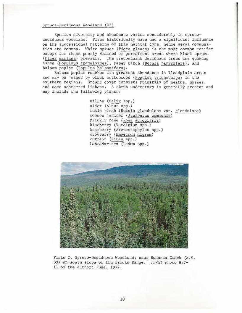
Spruce-Deciduous Woodland (02)
Species diversity and abundance varies considerably in sprucedeciduous woodland. Fires historically have had a significant influence on the successional patterns of this habitat type, hence seral communities are common. White spruce (Picea glauca) is the most common conifer except for those poorly drained or permafrost areas where black spruce (Picea mariana) prevails. The predominant deciduous trees are quaking aspen (Populous tremuloides), paper birch (Betula papyrifera), and balsam poplar (Populus balsamifera).
Balsam poplar reaches its greatest abundance in floodplain areas and may be joined by black cottonwood (Populus trichocarpa) in the southern regions. Ground cover consists primarily of heaths, mosses, and some scattered lichens. A shrub understory is generally present and may include the following plants:
willow (Salix spp.) alder (Alnus spp.) resin birch (Betula glandulosa var. glandulosa) common juniper (Juniperus communis) prickly rose (Rosa acicularis) blueberry (Vac~um spp.) bearberry (Arctostaphylos spp .) crowberry (Empetrum nigrum) currant (Ribes spp.) Labrador- tea (Ledum spp.)
Plate 2. Spruce-Deciduous Woodland; near Bonanza Creek (A.S. 89) on south slope of the Brooks Range. JFWAT photo 827-11 by the author; June, 1977.
10
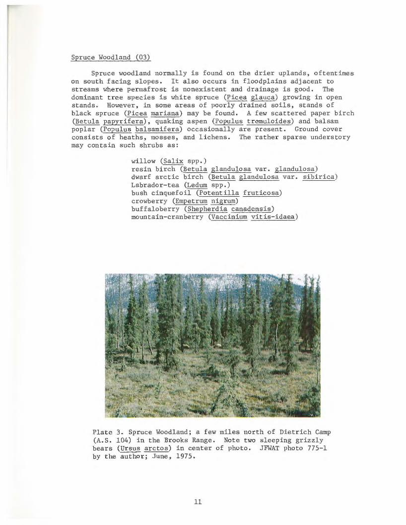
Spruce Woodland (03)
Spruce woodland normally is found on the drier uplands, oftentimes on south facing slopes . It also occurs in floodplains adjacent to streams where permafrost is nonexistent and drainage is good. The dominant tree species is white spruce (Picea glauca) growing in open stands . However, in some areas of poorly drained soils, stands of black spruce (Picea mariana) may be found. A few scattered paper birch (Betula papyrifera), quaking aspen (Populus tremuloides) and balsam poplar (Populus balsamifera) occasionally are present. Ground cover consists of heaths, mosses, and lichens. The rather sparse understory may contain such shrubs as:
willow (Salix spp . ) resin birch (Betula glandulosa var. glandulosa) dwarf arctic birch (Betula glandulosa var. sibirica) Labrador-tea (Ledum spp.) bush cinquefoil (Potentilla fruticosa) crowberry (Empetrum nigrum) buffaloberry (Shepherdia canadensis) mountain-cranberry (Vaccinium vitis-idaea)
Pl ate 3. Spruce Woodland; a few miles north of Dietrich Camp (A.S. 104) in the Brooks Range. Note two s leeping grizzly bears (Ursus arctos) in center of photo. JFWAT photo 775-1 by the author; June, 1975.
11
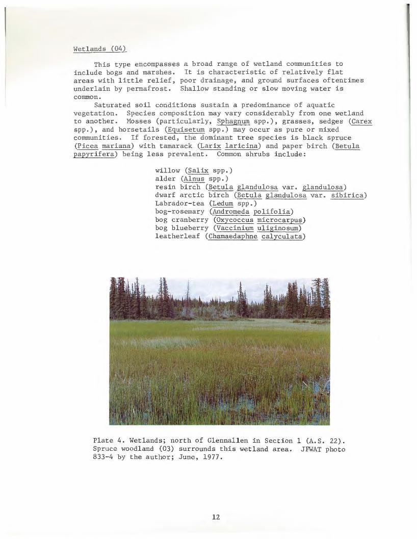
Wetlands (04)
This type encompasses a broad range of wetland communities to include bogs and marshes. It is characteristic of relatively flat areas with little relief, poor drainage, and ground surfaces oftentimes underlain by permafrost. Shallow standing or slow moving water is common.
Saturated soil conditions sustain a predominance of aquatic vegetation. Species composition may vary considerably from one wetland to another. Mosses (particularly, Sphagnum spp.), grasses, sedges (Carex spp . ), and horsetails (Equisetum spp.) may occur as pure or mixed communities. If forested, the dominant tree species is black spruce (Picea mariana) with tamarack (Larix laricina) and paper birch (Betula papyrifera) being less preval ent. Common shrubs include:
willow (Salix spp.) alder (Alnus spp . ) r esin birch (Betul~ glandulosa var. glandulosa) dwarf arctic birch (Betul a glandulosa var . sibirica) Labrador-tea (Ledum spp . ) bog-rosemary (Andromeda polifolia) bog cranberry (Oxycoccus microcarpus) bog blueberry (Vaccinium uliginosum) leatherleaf (Chamaedaphne calyculata)
Plate 4. Wetlands; north of Glennal len in Section 1 (A.S. 22 ). Spruce woodland (03) surrounds this wetland area. JFWAT photo 833- 4 by the author; June, 1977 .
12
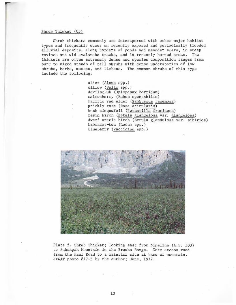
Shrub Thicket (05)
Shrub thickets commonly are interspersed with other major habitat types and frequently occur on recently exposed and periodically flooded alluvial deposits, along borders of ponds and meander scars, in steep ravines and old avalanche tracks, and in recently burned areas. The thickets are often extremely dense and species composition ranges from pure to mixed stands of tall shrubs with dense understories of low shrubs, herbs, mosses, and lichens. The common shrubs of this type include the following:
alder (Alnus spp.) willow (Salix spp.) devilsclub (Oplopanax horridum) salmonberry (Rubus spectabilis) Pacific red elder (Sambuscus racemosa) prickly rose (Rosa acicularis) bush cinquefoil (Potentilla fruticosa) resin birch (Betula glandulosa var. glandulosa) dwarf arctic birch (Betula glandulosa var. sibirica) Labrador- tea (Ledum spp.) blueberry (Vaccinium spp.)
Pl ate 5. Shrub Thicket; looking east from pipeline (A.S. 103) to Sukakpak Mountain in the Brooks Range. No t e access road from the Haul Road to a material site at base of mountain. JFWAT photo 817- 5 by the author; June, 1977.
13
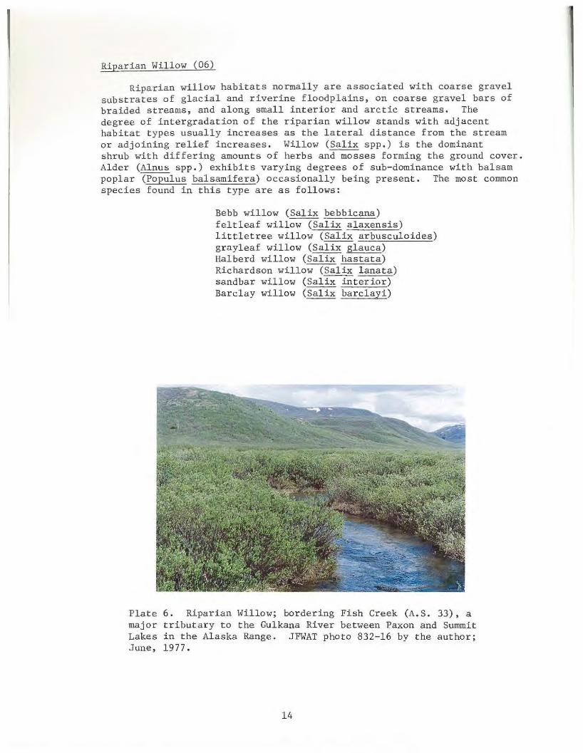
Riparian Willow (06)
Riparian willow habitats normally are associated with coarse gravel substrates of glacial and riverine floodplains, on coarse gravel bars of braided streams, and along small interior and arctic streams. The degree of intergradation of the riparian willow stands with adjacent habitat types usually increases as the lateral distance from the stream or adjoining relief increases. Willow (Salix spp .) is the dominant shrub with differing amounts of herbs and mosses forming the ground cover. Alder (Alnus spp.) exhibits varying degrees of sub-dominance with balsam poplar (Populus balsamifera) occasionally being present. The most common species found in this type are as follows:
Bebb willow (Salix bebbicana) feltleaf willow (Salix alaxensis) littletree willow (Salix arbusculoides) grayleaf willow (Salix glauca) Halberd willow (Salix hastata) Richardson willow (Salix lanata) sandbar willow (Salix interior) Barclay willow (Salix barclayi)
Plate 6. Riparian Willow; bordering Fish Creek (A.S. 33), a major tributary to the Gulkana River between Paxon and Summit Lakes in the Alaska Range. JFWAT photo 832-16 by the author; June, 1977.
14
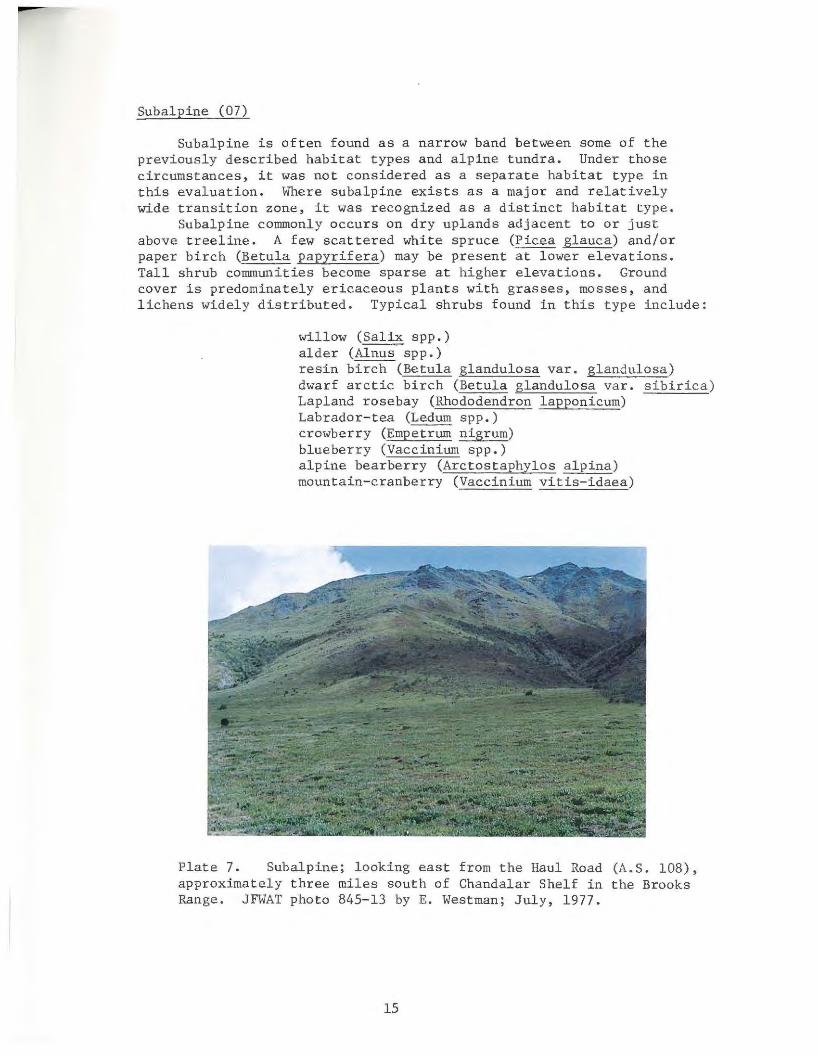
Subalpine (07)
Subalpine is often found as a narrow band between some of the previously described habitat types and alpine tundra. Under those circumstances, it was not considered as a separate habitat type in this evaluation. Where subalpine exists as a major and relatively wide transition zone, it was recognized as a distinct habitat type.
Subalpine commonly occurs on dry uplands adjacent to or just above treeline. A few scattered white spruce (Picea glauca) and/or paper birch (Betula papyrifera) may be present at lower elevations. Tall shrub communities become sparse at higher elevations. Ground cover is predominately ericaceous plants with grasses, mosses, and lichens widely distributed. Typical shrubs found in this type include:
willow (Salix spp.) alder (Alnus- spp.) resin birch (Betula glandulosa var. glandulosa) dwarf arctic birch (Betula glandulosa var. sibirica) Lapland rosebay (Rhododendron lapponicum) Labrador-tea (Ledum spp . ) crowberry (Empetrum nigrum) blueberry (Vaccinium spp.) alpine bearberry (Arctostaphylos alpina) mountain-cranberry (Vaccinium vitis-idaea)
Plate 7 . Subalpine; looking east from the Haul Road (A.S. 108), approximately three miles south of Chandalar Shelf in the Brooks Range. JFWAT photo 845-13 by E. Westman; July, 1977.
15
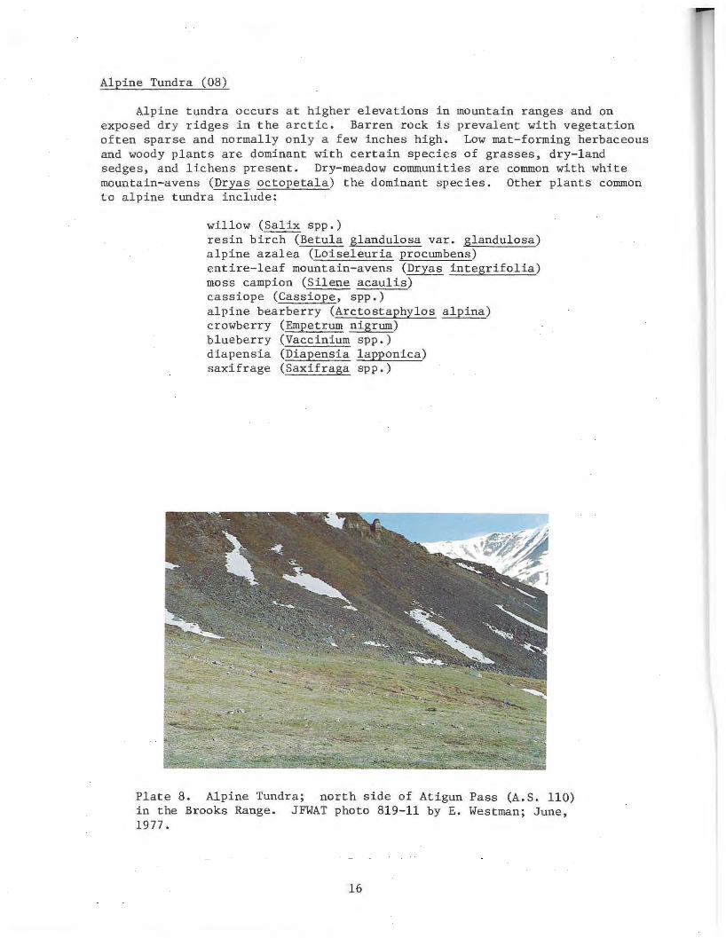
Alpine Tundra (08)
Alpine tundra occurs at higher elevations in mountain ranges and on exposed dry ridges in the arctic. Barren rock is prevalent with vegetation often sparse and normally only a few inches high. Low mat-forming herbaceous and woody plants are dominant with certain species of grasses, dry-land sedges, and lichens present. Dry-meadow communities are common with white mountain-avens (Dryas octopetala) the dominant species. Other plants common to alpine tundra include:
willow (Salix spp.) resin birch (Betula glandulosa var . glandulosa) alpine azalea (Loiseleuria procumbens) entire-leaf mountain-avens (Dryas integrifolia) moss campion (Silene acaulis) cassiope (Cassiope, spp . ) alpine bearberry (Arctostaphylos alpina) crowberry (Empetrum nigrum) blueberry (Vaccinium spp.) diapensia (Diapensia lapponica) saxifrage (Saxifraga spp.)
Plate 8 . Alpine Tundra; north side of Atigun Pass (A . S. 110) in the Brooks Range. JFWAT photo 819-11 by E. Westman; June, 1977.
16
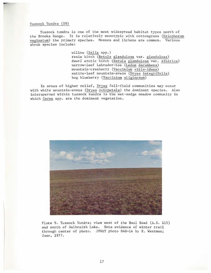
Tussock Tundra (09)
Tussock tundra is one of the most widespread habitat types north of the Brooks Range. It is relatively monotypic with cottongrass (Eriophorum vaginatum) the primary species. Mosses and lichens are common . Various shrub species include:
willow (Salix spp.) resin birch (Betula glandulosa var. glandulosa) dwarf arctic birch (Betula glandulosa var. sibirica) narrow-leaf Labrador-tea (Ledum decumbens) mountain-cranberry (Vaccinium vitis-idaea) entire-leaf mountain-avens (Dryas integrifolia) bog blueberry (Vaccinium uliginosum)
In areas of higher relief, Dryas fell-field communities may occur with white mountain-avens (Dryas octopetala) the dominant species. Also interspersed within tussock tundra is the wet-sedge meadow community in which Carex spp. are the dominant vegetation.
Plate 9. Tussock Tundra; view west of the Haul Road (A.S. 115) and north of Galbraith Lake. Note evidence of winter trail through center of photo. JFWAT photo 848-14 by E. Westman; June, 1977.
17
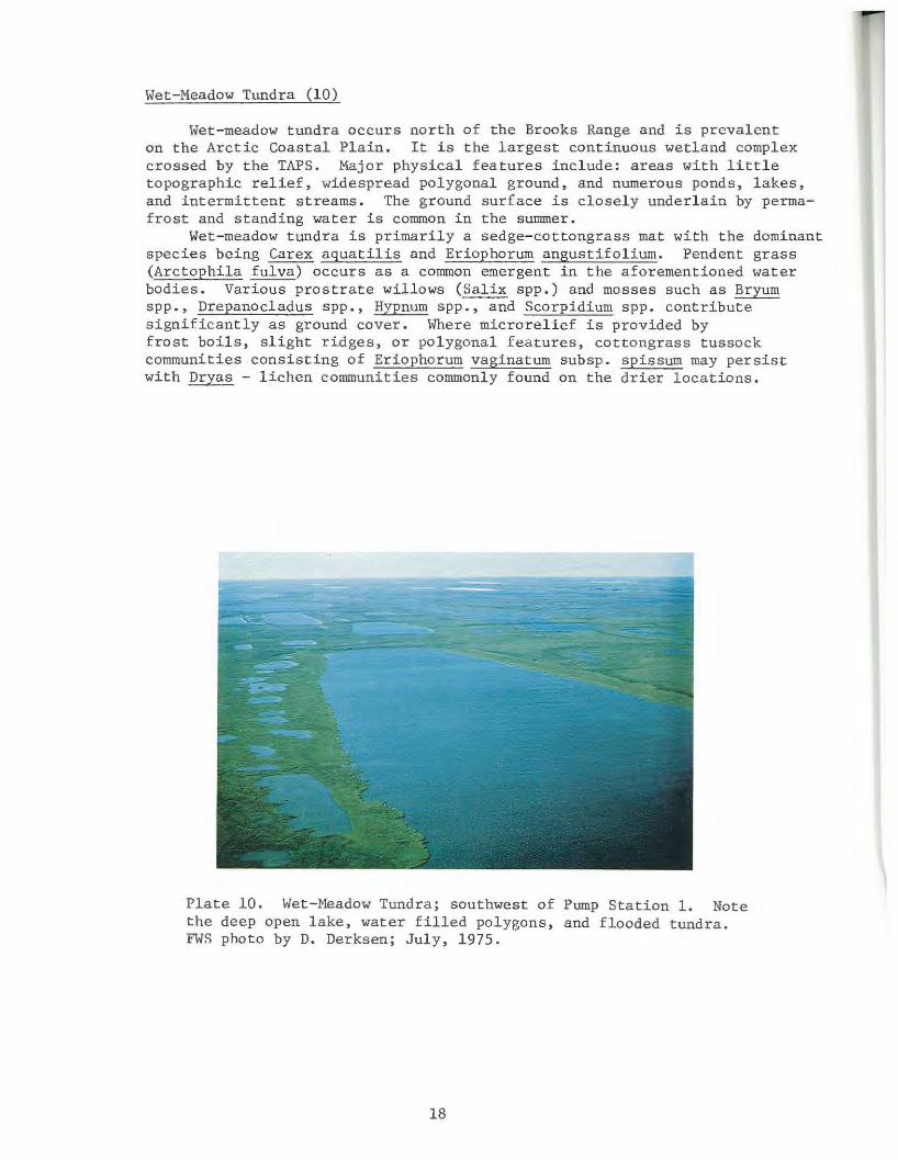
Wet- Meadow Tundra (10)
Wet-meadow tundra occurs north of the Brooks Range and is prevalent on the Arctic Coastal Plain . It is the largest continuous wetland complex crossed by the TAPS. Major physical features include: areas with little topographic relief, widespread polygonal ground, and numerous ponds, lakes, and intermittent streams. The ground surface is closely underlain by permafrost and standing water is common in the summer.
Wet-meadow tundra is primarily a sedge-cottongrass mat with the dominant species being Carex aquatilis and Eriophorum angustifolium. Pendent grass (Arctophila fulva) occurs as a common emergent in the aforementioned water bodies. Various prostrate willows (Salix spp.) and mosses such as Bryum spp . , Drepanocladus spp., Hypnum spp., and Scorpidium spp. contribute significantly as ground cover. Where microrelief is provided by frost boils, slight ridges, or polygonal features, cottongrass tussock communities consisting of Eriophorum vaginatum subsp. spissum may persist with Dryas - lichen communities commonly found on the drier locations.
Plate 10. Wet-Meadow Tundra; southwest of Pump Station 1. Note the deep open lake, water filled polygons, and flooded tundra. FWS photo by D. Derksen; July, 1975.
18
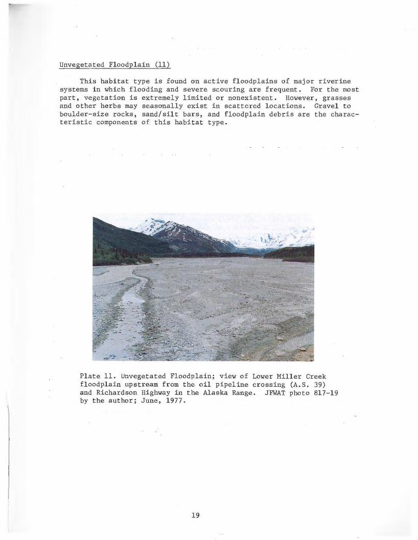
Unvegetated Floodplain (11)
This habitat type is found on active floodplains of major riverine systems in which flooding and severe scouring are frequent. For the most part, vegetation is extremely limited or nonexistent. However, grasses and other herbs may seasonally exist in scattered locations. Gravel to boulder- size rocks, sand/silt bars, and floodplain debr is are the characteristic components of t his habitat type.
Plat e 11. Unveget a t ed Floodplain; view of Lower Mill er Creek f l oodplain upstream from the oil pi peline crossing (A.S. 39) and Richardson Highway in the Alaska Range. JFWAT photo 817-19 by the author; June, 1977.
19
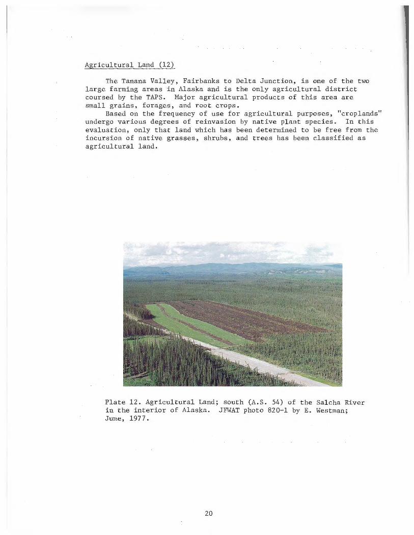
Agricultural Land (12)
The Tanana Valley, Fairbanks to Delta Junction, is one of the two large farming areas in Alaska and is the only agricultural district coursed by the TAPS. Major agricultural products of this area are small grains, forages, and root crops.
Based on the frequency of use for agricultural purposes, "croplands" undergo various degrees of reinvasion by native plant species. In this evaluation, only that land which has been determined to be free from the incursion of native grasses, shrubs, and trees has been classified as agricultural land.
Plate 12. Agricultural Land; south (A.S. 54) of the Sal cha River in the interior of Al aska. JFWAT photo 820-1 by E. Westman; June, 1977.
20
I ~
j
Quantitative Phase
Pre-Construction Imagery
In February, 1976, JFWAT acquired panchromatic black and white negatives of the TAPS corridor (scale 1:15,840) which had been taken aerially in 1969 and 1970. These negatives were used to produce an uncorrected 1:6,000 scale panchromatic black and white mosaic. This mosaic, comprised of 525 enlarged images, covered an area approximately 2.5 miles in width and extended the 800-mile length of the TAPS. The decision to use a large scale (i.e. 1:6,000) was prompted by the image dimensional characteristics of the TAPS construction impacts and the planimetric methodology that would be employed to measure those impacts.
Average Local Scale
An average scale normally is used to define the overall mean scale of a vertical photograph taken over variable terrain. Average scale is defined as the scale at the average elevation of the terrain covered by a specific photograph (Reeves et al. 1975). Since the pre-construction imagery was uncorrected for topographic variation, tilt, and radial distortion, an average local scale for each of the 525 images was determined. This was accomplished by calculating the mean for three separate scales identified at various locations on each pre-construction image. Each individual scale was derived by identifying the ratio of linear image distance to actual ground distance obtained from U.S. Geological Survey 1:63,360 scale topographic maps. Thus, the average local scale was more representative of the actual scale of each image than either the average scale of the entire image or the theoretical scale at the photograph's principle point.
Photo Interpretation
Conventional methods of aerial photographic interpretation were used to identify and delineate the twelve habitat (vegetation) types on the pre-construction aerial photographs. By evaluating image characteristics and collateral data (e.g. ground data), habitat delineations were made directly on the enlarged aerial photographs with a mechanical grease pencil. This technique permitted the revision of interpretations and avoided damaging the photographic image. Revisions were made as ground data were accumulated and changes in interpretations were warranted.
Although the twelve habitat types were general, the delineations of type boundaries were quite specific. For the most part, distinct habitats of three or more acres were cover typed. In some instances, dependent on image quality, it was possible to delineate habitat types as small as one acre.
21
A two-digit habitat type code was inscribed within the habitat-type boundary on the imagery. In developed areas where man-caused actions had resulted in the removal of all vegetation, the code "CL11 (cleared) was marked within the delineated boundary of the developed area. Airstrips, mine tailings, roads, and community developments are representative of the types of disturbances identified in this manner and were not included in the evaluations and computations.
Although each photographic enlargement was interpreted individually, the overlapping sections of adjacent enlargements were concurrently interpreted stereoscopically. By using this approach, habitat-type delineations that traversed overlapping image areas of adjacent enlargements had the same type boundaries.
Once each photographic enlargement had been interpreted, an edit was made to ensure that all habitat boundary lines were complete and the appropriate habitat codes marked within the delineated habitat types. After all collateral data had been compiled and analyzed, a final edit was conducted of all habitat interpretations and delineations for each pre-construction enlargement.
Collateral Data
Throughout the photo interpretation process, supportive information (i.e. collateral data) was used to facilitate the identification and delineation of the habitat types. Sources of collateral data included:
(1) color infrared vertical aerial photographic imagery, (2) color and panchromatic black and white vertical aerial
photographic imagery, (3) color and panchromatic black and white 35mm oblique
photographs, (4) aerial and on-the-ground field observations collected by
JFWAT personnel, and (5) miscellaneous cartographic material.
Emphasis for collection of ground data was placed on making numerous observations rather than relying upon a limited number of defined sample sites. This rationale was based on three factors:
(1) the large size of the study area, (2) the generality of the twelve habitat types, and (3) personnel and timetable limitations.
Ground data were collected by ocular inspection and plants identified with the aid of vegetation identification keys (e.g. Hulten [1968] and Welsh [1974]). The principal photo interpreter participated in the acquisition of ground data. Habitat type observations were made from the ground or during aerial flights and were recorded on 1:12,000 scale
22

base maps. Ground data were collected primarily during the summer field seasons of 1976 and 1977. A total of 6,321 field observations were obtained, approximately 35% aerially and 65% ground.
Overlay Preparation
Following the interpretation and delineation of habitat types on pre-construction imagery, transparent mylar overlays were prepared. The mylars were trimmed to the same dimensions as the pre-construction aerial photographs. After cataloging each overlay to coincide with the appropriate enlargement, the habitat-type delineations were traced and codes marked on the overlay. Terrain features that would facilitate correct alignment of the overlay upon post-construction images were identified on the mylar overlays. Relatively static features, such as lakes and man-made clearings, provided alignment guides for the placement of pre-construction habitat-type overlays upon post-construction photographic enlargements. The function of the overlays was limited to the transfer of pre-construction habitat information to post-construction imagery enlarged to the same scale.
Post-construction Imagery
In order to compare pre- and post-construction imagery, panchromatic black and white negatives (scale 1:36,000), taken aerially in June and July 1976, were enlarged approximately six times using a commercial enlarger. By using a pre-construction image of the same area as an enlarging guide, post-construction imagery of the same scale was produced. This was done to allow the direct comparison of pre-construction habitattype overlays with enlarged post-construction imagery. Post-construction imagery of the TAPS consisted of 362 panchromatic black and white photographic enlargements with an approximate scale of 1:6,000.
Areal Calculation of Construction-Related Impacts
APSC "G-5" technical drawings and field documentation by JFWAT monitors were used to identify the various components (e.g. work pad, material sites, camps, etc.) of TAPS construction-related impacts (Appendix V, Plates 15 - 34) on the post-construction imagery. It should be stressed that a conservative approach was taken in quantifying impacts. If there were questions as to whether or not a particular impact was TAPS associated, the impact was not included.
Following identification of construction-related impacts on postconstruction imagery, the pre-construction habitat type overlays, having the same scale as the post-construction imagery, were aligned with the appropriate post-construction image. In this manner, the pre-construction overlays revealed the habitat types prior to TAPS construction.
23
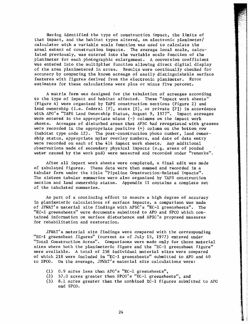
Having identified the type of construction impact, the limits of that impact, and the habitat types altered, an electronic planimeter/ calculator with a variable scale function was used to calculate the areal extent of construction impacts. The average local scale, calculated previously, was entered into the variable scale function of the planimeter for each photographic enlargement. A conversion coefficient was entered into the multiplier function allowing direct digital display of the area planimetered in acres. Resul~s were continually checked for accuracy by comparing the known acreage or easily distinguishable surface features with figures derived from the electronic planimeter. Error estimates for these calculations were plus or minus five percent.
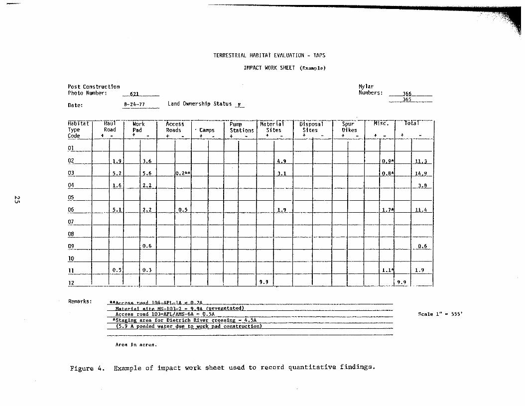
A matrix form was designed for the tabulation of acreages according to the type of impact and habitat affected. These "impact work sheets" (Figure 4) were organized by TAPS construction sections (Figure 2) and land ownership (i.e. federal [F), state [S], or private [P]) in accordance with APO's "TAPS Land Ownership Status, August 9, 1977". Impact acreages were entered in the appropriate minus (-) columns on the impact work sheets. Acreages of disturbed areas that APSC had revegetated with grasses were recorded in the appropriate positive (+) column on the bottom row (habitat type code 12). The post-construction photo number, land ownership status, appropriate mylar overlay numbers, and date of data entry were recorded on each of the 414 impact work sheets. Any additional observations made of secondary physical impacts (e.g. areas of ponded water caused by the work pad) were measured and recorded under "remarks".
After all impact work sheets were completed, a final edit was made of tabulated figures. These data were then summed and recorded in a tabular form under the title "Pipeline Construction-Related Impacts". The sixteen tabular summaries were also organized by TAPS construction section and land ownership status. Appendix II contains a complete set of~the tabulated summaries.
As part of a continuing effort to ensure a high degree of accuracy in planimeteric calculations of surface impacts, a comparison was made of JFWAT's material site findings with APSC's "EC-1 greensheets". The "EC-1 greensheets" were documents submitted to APO and SPCO which contained information on surface disturbance and APSC's proposed measures for rehabilitation and restoration.
JFWAT's material site findings were compared with the corresponding "EC-1 greensheet figures" (current as of July 15, 1977) entered under "Total Construction Acres". Comparisons were made only for those material sites where both the planimeteric figure and the "EC-1 greensheet figure" were available. A total of 258 individual material sites were compared of which 218 were included in "EC-1 greensheets" submitted to APO and 40 to SPCO. On the average, JFWAT's material site calculations were:
(1) 0.9 acres less than APO's "EC-1 greensheets", (2) 57.0 acres greater than SPCO's "EC-1 greensheets", and (3) 8.1 acres greater than the combined EC-1 figures submitted to APO
and SPCO.
24
N \J1
TERRESTRII\L 11/\0ITAT EV/\LUI\TION - TI\PS
H1PACT WORK SHEET (F.xample)
Post Construction Mylar Photo Number: _6.21 __ _ Numbers: __ Jf!L __
Date: 8-24-77 Land Ownership Status _r_ ______m __ _
Habitat flaul Work Access Pump Material ~-· Misc. Iota! Disposal Spur Type Road Pad Roads · Camps Stations Sites Sites Dikes Code + - + - + - + - + - + - + - + - + - + - ·-01
02 .L.2. -- h6 4.9 ~. '--- .JL.L
~- 5.2 5.6 0.2"'* J.L - J)_.8* lhl_ --04 - 1.6 2.2 -~..JL ----05 .
06 5.1 2.2 0.5 1.9 1. 7"' 11.4
07 ·- ·--- - ---08 '---·
09 0.6 0.6 -10 -11 0.5 O.J 1.1 1.9
12 ' 9.9 9.9
·-·- ------· .....- ·---···--
Remarks: ..M,A=ess road 104-API.-Material sJ te MS-101-2 c 9..!1A._(Revegetnte<!l. ___________________ _ Access road 10J=APL/AMS-6A = 0.5A Scale 1" = 555'
*Staging area for Dietrich River crossing - 4.5A (5.9 A ponded water due to work pad construction)
Area :In acres.
Figure 4. Example of impact work sheet used to record quantitative findings.
Qualitative Phase
General
In the past few years, several state fish and wildlife agencies, private conservation organizations, and the FWS have been working cooperatively to develop a habitat evaluation system for determining the effects of water-related development projects on fish and wildlife resources (Flood et al. 1977). Although interim products are now available (usm~s 1976), standardized procedures for evaluating potential impacts of major projects on fish and wildlife habitats have not been finalized. JFWAT's efforts to evaluate and document the overall impacts of a major construction project (TAPS) were unprecedented in Alaska.
Without a basic understanding of the qualitative values associated with wildlife habitats, knowledge of quantified habitat losses is meaningless. The primary purpose of the qualitative phase was to determine the overall value or quality of each of the twelve habitat types relative to the myriad of wildlife species which these habitats support. To accomplish this task, a systematic and empirical approach was used.
Representative Wildlife Families/Species
A literature review was conducted to obtain an understanding of the existing data base relative to the habitat requirements and preferences of Alaskan wildlife species common to the TAPS corridor. The objective was to focus on wildlife in general with no preference toward any particular group (i.e. big game, small game, furbearers, etc.) Based on this review six major wildlife groups were chosen: large mammals, small mammals, birds of prey, upland birds, waterfowl, and other water/marsh birds. Families of each group were analyzed and four families were selected to represent each group. Based on distribution, adaptability, status, seasonality, and differing habitat requirements, species within each family were chosen as the "Wildlife Evaluation Elements" (Appendix III). The selection of wildlife families and species was directed at obtaining a representative cross-section of the wildlife community such that a broad basis could be used to evaluate habitat quality. Information sources used in this part of the evaluation are included in the "References" section.
Biological Parameters
For each selected wildlife species, a detailed literature review was conducted to compile ·available data concerning habitat requirements and preferences. The information was categorized by three basic biological parameters (food, cover, and reproduction) and analyzed for each wildlife species. A fourth parameter, migration/movement, was included initially, but was dropped from the evaluation due to insufficient information in the literature relative to habitat types.
26
Life-support requirements and habitat preferences oftentimes vary between wildlife species with differences being much greater when species are from different families. Depending on the species, food sources may be comprised of plants, animals, or a combination of these sources. For each species selected, data on food sources included, when appropriate, the following items:
(1) types of plants, (2) parts of plants (e.g. stems, buds, leaves, fruit, and seeds), (3) animal prey (e.g. adults, young, avian eggs), and (4) miscellaneous items such as invertebrates and carrion.
As with food, the availability and quality of cover is important to wildlife. Cover is used for various functions to include:
(1) escape from natural enemies, (2) concealment, (3) shelter from adverse environmental conditions, (4) resting, and (5) performance of bodily maintenance (e.g. grooming, preening, molting).
When gathering information on cover requirements, both living and dead vegetation were considered. For example, ground cover is composed not only of living plants but also may contain fallen leaves, branches, and tree trunks. Other cover features such as rock structures, bluffs, and streambanks also were noted.
Successful reproduction by a wildlife population is related closely to the quantity and quality of food and cover. In addition, other reproductive requirements vary depending on the species and may include:
(1) adequate nest sites (e.g. evergreen trees, tall shrubs, hollow logs), (2) availability of materials to construct nests (e.g. sticks, leaves,
grasses), (3) calving or lambing areas, (4) den sites, and (5) rearing areas (e.g. waterfowl brood rearing).
Determination of Habitat Quality
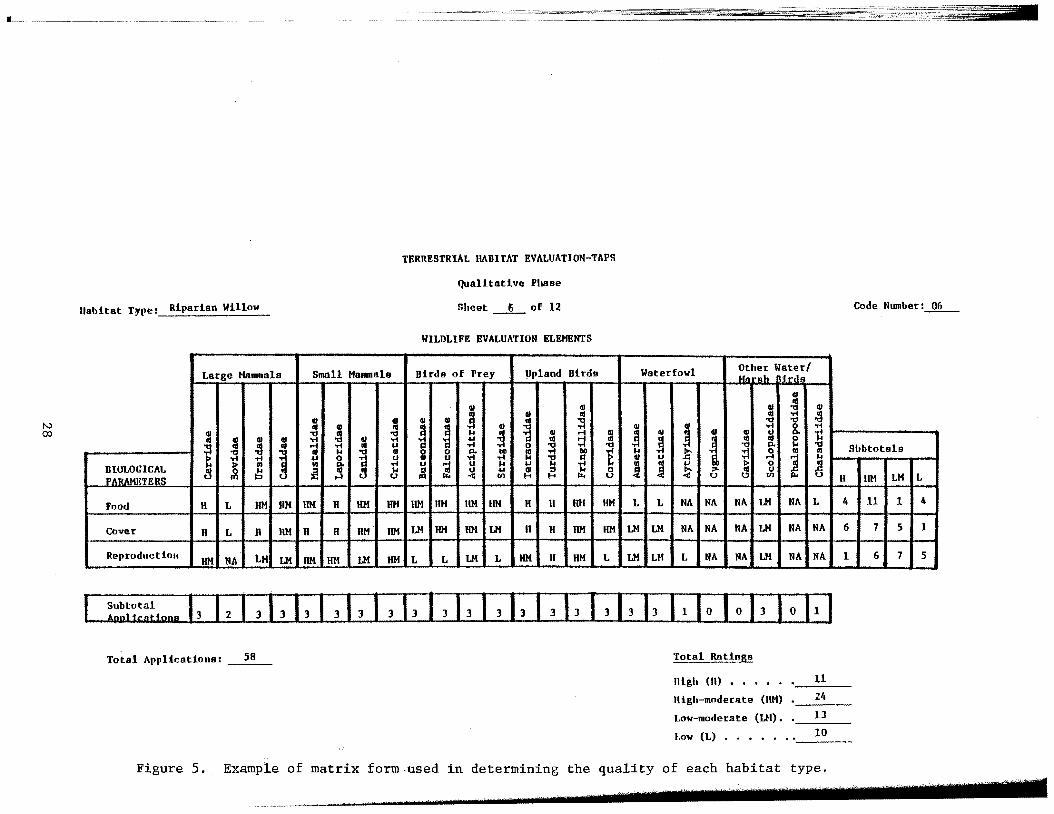
A matrix form (Figure 5) was used in assessing the quality of each habitat type. Habitat types were evaluated independently in order to minimize bias relative to comparing habitats. For each type, an analysis was made of the potential capability of that habitat to provide the necessary food, cover, and reproduction requirements for each of the wildlife evaluation elements. In addition to evaluating each habitat type, the ecological relationships of the terrestrial types when interfacing with freshwater aquatic communities (e.g. ponds, lakes, and streams) were considered. Rating categories for expressing these relationships were:
{1) high, (2) high-moderate, (3) low-moderate, and (4) low.
27
L .. -
TERRESTRIAL HABITAT EVALUATION-TAPS
Qualitative Phase
Uabitat Trpe: Riparian Willow Sheet _6_ of 12 Code Number:~
WILDLIFE EVALUATION ELEMENTS
Large Ma11111als Small Malllllals Birds of Prey Upland Birds Waterfowl Other Water/ MArAb Urds
41
j 41 = ~ 41
Ill ~ -3 ., = " Ill
~ ;t 'tl 'tl
-3 ~ ! ~ .. J
41 Ti 0 Ti
" ;t k
~ = a = 41
~ Ill .. i
p. 'U ~ :1 ~ : ...t :1 4.1
~ i Ill 0
;t .-! Ti 4.1 1'1 Ti 0 ;t 'tl 'tl k 'tl Subtotals ;t ] Ill ,.. 'tl 41 2 0 ;r 1>0 ~ 1>0 t k .t' :;1 !\ Ill j ~ ...t 4.1 0 s ~ 0 Ti 'tl J:l 41 4.1
~ BIOLOGICAL ! !II Ill ~ .., .-! 0 tl
.., ,.. ...t i i ..,
~ 0
~ :i1 k a ~ .<.1 ~ ::s J:: 0 ~ ;o. u PARAMI~TERS
u o-1 u (I} ..,. u u tl) II liM LM L
Food H L HM HM liM H HM HM HM HM liM liM II ll Htl HM L L NA NA NA LM NA L 4 11 1 4
Cover II L H HM H H liM JIM LM HM HM LM lt H liM HM LM LM NA NA NA LM NA NA 6 7 5 1
Reproduction HM NA LM LM liM HM LM HM L L LM L HM II HM L LM LM L NA NA LM NA NA 1 6 7 5
Total Applications: __ 5_8_ Total Ratings
II igh (II) • • • 11
High-moderate (liM) • 24
{,ow-moderate (UI). • 13
l.ow (L) 10 ..... ··-----
Figure 5. _ Example of matrix form used in determining the quality of each habitat type.
An "NA" (non-applicable) was entered whenever a particular biological parameter did not apply to a certain evaluation element for a specific habitat type or if the wildlife use of that habitat type for a particular parameter was relatively insignificant.
Eight JFWAT biologists conducted independent qualitative evaluations of each of the twelve habitat types. The results of these evaluations were correlated with data obtained from the literature review to yield a subjective rating for each of the 24 wildlife evaluation elements relative to the three biological parameters for each habitat type. The total number of times which a rating category was entered across the evaluation elements for a particular biological parameter was totaled on the right side of the matrix form. The number of applications (rating entries minus "NA's") were totaled under each evaluation element column. The total applications and ratings were summed for each habitat type.
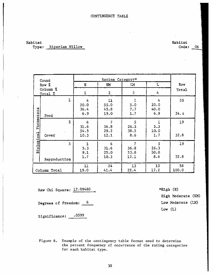
In order to quantitatively analyze the ratings of habitat quality, standard statistical procedures were employed. Contingency tables (Figure 6) were developed for the twelve habitat types. These tables display the percent frequency of occurrence of the rating category subtotals (Figure 5). Using this procedure, the overall differences between the ratings of the three biological parameters could be determined for each habitat type. This is reflected by the raw chi square values and their corresponding levels of significance. Thus, the most important aspects of each habitat type relative to its ability to provide the necessary habitat requirements for a broad spectrum of wildlife species were identified.
A contingency table was developed for the twelve habitat types in relation to the overall rating categories and a significant difference was found using a chi square test. A series of multiple range tests (Least Significant Difference [LSD], Tukey-Honest Significant Difference, and Scheffe) were conducted for the purpose of rank ordering the habitat types according to habitat quality. The resulting groups were comprised of habitat types which were not significantly different in their overall ratings. For each group, the mean, standard deviation, and standard error were calculated.
FINDINGS
Habitat Typing
As a result of cover typing the study area on pre-construction aerial photographs, a mosaic of habitat types was produced which is equivalent to approximately 2,150 square miles. This area is equal to approximately 1.37 million acres (an area slightly larger than the State of Delaware). Since the habitat typing data cannot be provided in this report, a brief discussion of the results follows in order to provide an overview of the geographical and areal extent of habitats delineated based on the classification system used in this evaluation.
29
CONTINGENCY TABLE
Habitat Habitat Code: Type: Riparian Willow
I
I
Count Row% H Column % Total % 1
]._ 4 20.0
Ill 36.4 M (1) 6.9 ~ Food (1) c: c:a 2 6 M co 31.6 p..
~ 54.5
d Cover 10.3 ~
o-f
g: 3 1 ..-1 0 5.3 -I:Q 9.1
Reproduction 1.7
11 Column Total 19.0
Raw Chi Square: 12.09480
Degrees of Freedom: 6
Significance: .0599
Ratin~ CategorY* HH L'1
2 3
11 1 55.0 5.0 45.8 7.7 19.0 1.7
7 5 36.8 26.3 29.2 38.5 12.1 8.6
6 7 31.6 36.8 25.0 53.8 10.3 12.1
24 13 41.4 22.4
L Row Total
4
4 20 20.0 40.0 6.9 34.4
1 19 5.3
10.0 1.7 32.8
5 19 26.3 50.0 8.6 32.8
10 58 17.2 100.0
*High (H)
High Moderate (HM)
Low Moderate (~)
Low (L)
Figure 6. Example of the contingency table format used to determine the percent frequency of occurrence of the rating categories for each habitat type.
30
Section 1 - Terrestrial habitats found in the Valdez Terminal area (Figure 2) are primarily coastal forest and shrub thickets. Alpine tundra exists at the higher elevations but was not directly affected by the construction of the terminal facilities. Coastal forest extends northward from the Terminal through Section 1 for approximately 25 miles where it is replaced by sprucedeciduous woodland and spruce woodland north of Thompson Pass in the Chugach Mountains. Shrub thickets often occur in large expanses and unvegetated floodplains are common along the major river systems. Subalpine habitats are scattered throughout the mountainous regions of the section and alpine tundra is prevalent at higher elevations. Spruce-deciduous woodland is more common than spruce woodland, especially in the southcentral portion of Section 1. Wetlands occur periodically and increase in size and number from the central to the northern portions of the section.
Section 2 - Spruce woodland occurs more frequently than spruce-deciduous woodland. Shrub thickets and riparian willow are common throughout this section and are especially prevalent in the southern foothills of the Alaska Range. Subalpine is common along the TAPS through the Alaska Range with alpine tundra occurring at higher elevations. Wetlands commonly are interspersed with other habitat types, particularly spruce woodland. Unvegetated floodplains occur in the major drainages, especially along the Delta and Tanana Rivers. Agricultural lands are found primarily in the northern portion of Section 2.
Section 3 - The most widespread habitats are spruce-deciduous woodland and spruce woodland. Shrub thickets are more prevalent than riparian willow in this portion of the study area with the latter habitat normally occurring as narrow bands along small streams. Agricultural lands and unvegetated floodplains occur in the southern portion of this section. There are no developed agricultural lands north of Section 3. Rolling hills and low-elevation mountains exist in the central and northern portions of Section 3 and subalpine habitats are relatively small and scattered; alpine tundra was not found in this section. Wetlands are relatively widespread in the southern portion of this section but are restricted primarily to lowlands in the northern portion.
Section 4 - Both spruce-deciduous woodland and spruce woodland are found with the latter becoming more widespread in the central and northern portions of the section. Wetlands are found mainly in the lowlands and adjacent to low-gradient streams. Riparian willow and shrub thickets are interspersed throughout the section. A large expanse of subalpine habitat occurs in the northcentral portion with alpine tundra becoming prevalent at higher elevations on the south slope of the Brooks Range. Unvegetated floodplains occur in the Middle Fork Koyukuk drainage. Relatively small areas of tussock tundra are found in parts of this section.
Section 5 - Spruce-deciduous woodland and spruce woodland occur in the southern and central portions of Section 5 with both habitat types reaching their northernmost extent in this section. Riparian willow and
31
shrub thickets are both prevalent with the former type common along small streams and on floodplains of the Dietrich and Atigun Rivers. Subalpine occurs as a common transition type in this portion of the Brooks Range with alpine tundra found at higher elevations throughout the section. Wetlands are usually small but frequently occur in the lowlands and areas adjacent to small streams and side channels of larger rivers. Tussock tundra becomes widespread at lower elevations on the north side of the Continental Divide.
Section 6 - Tussock tundra is prevalent in the southern and central portions of Section 6 with wet~eadow tundra becoming essentially a monotype in the northern portion of the section. Alpine tundra occurs on the higher elevations in the southern part of the section with wetlands normally existing in areas with little topographic relief in the southern and central portions. Shrub thickets and riparian willow are found throughout the section with the latter being common along small streams and in the floodplains of major drainages, particularly the Sagavanirktok River.
As previously discussed, the delineations of habitat type boundaries on the pre-construction imagery were quite specific. An analysis was not made of the degree and frequency of interspersion of the various habitat types. However, an 11% systematic random sample of the aerial imagery was selected and analyzed to determine the mean linear distance of the transition zone between different habitat types. The overall mean width of habitat transition zones (as derived from the accumulated data of 53 enlargement sample means) was 237 feet.
Habitat Quality
Copies of the completed matrix forms and corresponding contingency tables, used in determining the overall quality of each habitat type, are contained in Appendix IV. The overall relationships of the various biological parameters to the wildlife evaluation elements for each particular habitat type are shown in the contingency tables. They illustrate consistency within a given type, as well as identify the biological parameter(s) which is (are) most important for wildlife with respect to the type's ability to fulfill the habitat requirements. By reviewing the contingency table for each habitat type, it becomes clear that an evaluation of habitat quality should not be based solely on a single biological parameter nor on a limited number of wildlife evaluation elements.
In the case of riparian willow, there were 20 (34.4%) rating entries made for food (out of a possible 24 wildlife evaluation elements) and 19 (32.8%) entries for both cover and reproduction (Figure 6). A review of the "column totals" shows a significantly greater number of high-moderate ratings (41.4%) than any other rating category. The chi square value (12.09380) is significant at .0599, thereby indicating that this habitat
32
type is inconsistent in providing the food, cover, and reproduction requirements of the selected wildlife families/species. The "column %" figures for food show 36.4% of the ratings as high and 45.8% highmoderate. Cover is 54.5% high and 29.2% high-moderate. Reproduction shows only 9.1% of the ratings high with 25.0% high-moderate. Thus, while riparian willow provides relatively equal numbers of wildlife evaluation elements with food, cover, and reproduction requirements, the quality of these parameters is not uniform. However, its overall ability to fulfill the habitat requirements of a wide range of wildlife families is relatively high as reflected by 60.4% of the ratings being high or high-moderate.
Unlike riparian willow, agricultural land is consistent in the rating of the biological parameters; the overall ratings are low (Appendix IV). Agricultural land has 97.3% of the ratings under "column total" as low or low-moderate. Food is the only biological parameter of any importance relative to agricultural land's ability to provide the habitat needs of the wildlife evaluation elements.
For wet-meadow tundra (Appendix IV), the overall rating is high as shown by a combined "column total" of 72.0% for high or high-moderate. The ratings are also consistently high for all biological parameters. The .3606 significance level indicates little variability between the ratings of the biological parameters. The number of rating entries, as shown in the "row total", is less for reproduction (26.4%) than either food or cover. Thus, the reproductive needs of the wildlife evaluation elements are met for a smaller number of elements than the corresponding food and cover requirements for the same elements.
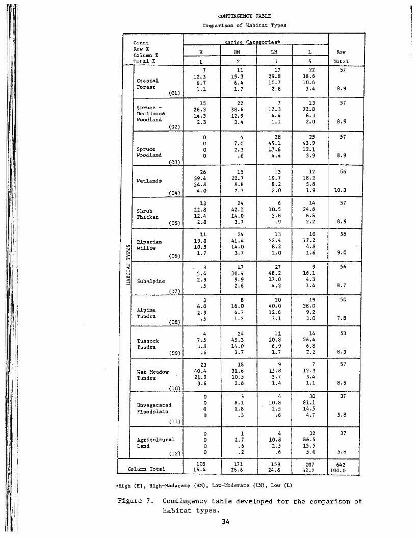
The contingency table for comparing the twelve habitat types is shown in Figure 7. The overall ratings of each habitat type and the consistency of ratings between the biological parameters for each type are incorporated in this table. The significance level of 0.0 indicates an extreme variability between the habitat types.
The greatest number of high ratings were for wetlands and wetmeadow tundra. Unvegetated floodplain and agricultural land received the greatest number of low ratings. Shrub thicket, riparian willow, and tussock tundra each had the same percentage of high-moderate ratings. The greatest number of low-moderate ratings occurred in spruce woodland, subalpine, and alpine tundra.
Relative to the 642 total applications, the low rating category for agricultural land occurred more frequently (5.0%) in the overall evaluation of biological parameters than any other rating category for any particular habitat type. The low ratings for unvegetated floodplain were next, followed by the high ratings for wetlands.
The multiple range tests (used for one-way analysis of variance of the ratings in the above contingency table) had different criteria for rank ordering the twelve habitat types. The LSD test was the most
33
Count Row% Colunm % Total %
Coastal Forest
(01)
Spruce -Deciduous Woodland
{02)
Spruce Woodland
(03)
Wetlands
(04)
Shrub Thicket
(05)
Riparian C/l Willow :.l
"" (06) ..... E-<
~ E-< .... ::::1
~ Subalpine
(07)
Alpine Tundra
(08)
Tussock Tundra
(09)
Wet: Meadow Tundra
(10)
Unvegetated Floodplain
(11)
Agricult:ural Land
(12}
Colunm Total
CONTDIGENCY TABLE
Comparison of Habitat Types
lt:•rin<> teat" •!>'ori<>"'*
H HM LM
1 2 3
7 11 17 12.3 19.3 29.8 6.7 6.4 10.7 1.1 1.7 2.6
15 22 7 26.3 38.6 12.3 14.3 12.9 4.4
2.3 3.4 1.1
0 4 28 0 7.0 49.1 0 2.3 17.6 0 .6 4.4
26 15 13 39.4 22.7 19.7 24.8 8.8 8.2 4.0 2.3 2.0
13 24 6 22.8 42.1 10. s 12.4 14.0 3.8
2.0 3.7 .9
u 24 13 19.0 41.4 22.4 10.5 14.0 8.2 1.7 3.7 2.0
3 17 27 5.4 30.4 48.2 2.9 9.9 17.0
.5 2.6 4.2
3 8 20 6.0 16.0 40.0 2.9 4.7 12.6 .s 1.2 3.1
4 24 11 7.5 45.3 20.8 3.8 14.0 6.9
.6 3.7 1.7
23 18 9 40.4 31.6 15.8 21.9 10.5 5.7 3.6 2.8 1.4
0 3 4 0 8.1 10.8 0 1.8 2.5 0 .5 .6
0 1 4 0 2.7 10.8 0 .6 2.5 0 .2 .6
105 171 159 16.4 26.6 24.8
*High (R) , High-Moderate (HM), LoY-'·!oderat:e (!...'!:} , Lo~.r (L)
L Row
4 Total
22 57 38.6 10.6 3.4 8.9
13 57 22.8 6.3 2.0 8.9
25 57 43.9 12.1
3.9 8.9
12 66 18.2
5.8 1.9 10.3
14 57 24.6 6.8 2.2 8.9
10 58 17.2
4.8 1.6 9.0
9 56 16.1 4.3 1.4 8.7
19 50 38.0
9.2 3.0 7.8
14 53 26.4 6.8 2.2 8.3
7 57 12.3
3.4 1.1 8.9
30 37 81.1 14.5
4.7 5.8
32 37 86.5 15.5 5.0 5.8
207 642 32.2 100.0
Figure 7. Contingency table developed for the comparison of habitat types.
34
1 l i
conservative while the Scheffe test was the most liberal. Based on significant differences, the results of all multiple range tests clearly indicated two extreme habitat groups; one composed of wetlands and wetmeadow tundra and the other composed of unvegetated floodplain and agricultural land. Regardless of the test procedure, the other habitat types remained in the same order, but different groups resulted depending upon the significance level applied in each test.
After analyzing the various test results, the most conservative test (the LSD) was selected for rank ordering the habitat types in relation to their overall habitat quality. The groups were differentiated based on their overall ratings and the degree of consistency in rating. The LSD test identified five groups which were significantly different at the .100 level (Figure 8). The habitat types in Group I are considered to be high quality (HQ) wildlife habitats, Those in Group II are high-medium quality (HMQ) and Group III types are medium quality (MQ). The habitat types in Group IV are low-medium quality (LMQ) and those in Group V are low quality (LQ) wildlife habitats. Hereafter in this report, a reference will be made to the habitat quality immediately following the name of the habitat type (e.g. wetlands [HQ]).
Construction-Related Impacts
As previously noted, summary sheets of TAPS construction-related impacts on terrestrial wildlife habitats are contained in Appendix II. The impacts are recorded by pipeline construction section (Figure 2) and land ownership. It should be re-emphasized that a conservative approach was used in determining TAPS impacts. Also, construction of the TAPS was not complete at the time (July, 1976) the "post-construction" photographs were taken. The author estimates that approximately 95% of the surface disturbances associated with TAPS construction occurred prior to July, 1976. A few of the twelve pump stations (Plates 27 & 28) had not been constructed or were partially constructed (e.g. Pump Stations 2 and 7). Numerous spur dikes (Plates 24 & 29) were not constructed, particularly in Sections 5 and 6. A few material sites (Plates 29 - 34) were expanded after the photography date. The facilities at the Valdez Terminal (Plate 23) were not complete. The Haul Road· (Plates 15, 16 & 21), access roads (Plates 21, 32, & 34), work pad (Plates 17-21 & 24), and camps (Plates 25 & 26) had been constructed.
Impacts By Land Ownership
Approximately two-thirds of the lands crossed by TAPS were federally owned. Slightly less than one-third were state lands, and the remaining lands were privately owned. Impacts by construction section on federal, state, and private lands are shown in Tables 1, 2, and 3, respectively. A summary of the impacts to the twelve habitat types according to land ownership is shown in Table 4. TAPS construction on federal lands
35
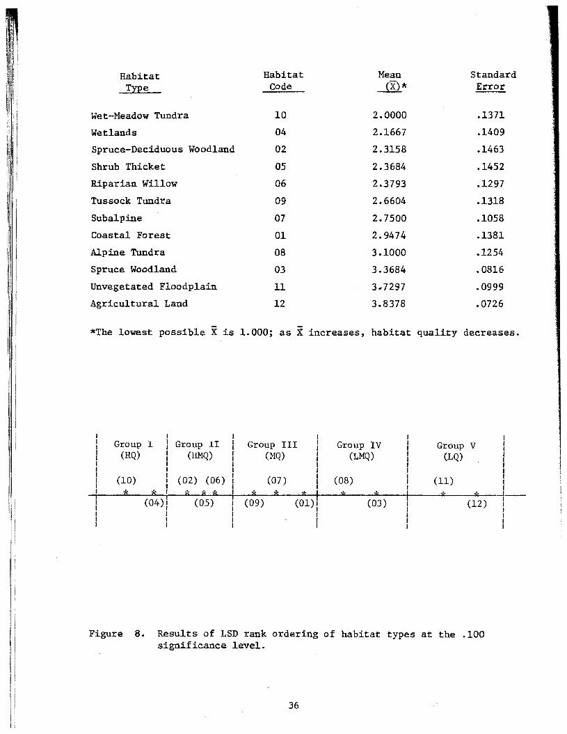
Habitat Habitat Mean Standard TYPe Code (X)* Error
Wet-Meadow Tundra 10 2.0000 .1371
Wetlands 04 2.1667 .1409
Spruce-Deciduous Woodland 02 2.3158 .1463
Shrub Thicket 05 2.3684 .1452
Riparian Willow 06 2.3793 .1297
Tussock Tundra 09 2.6604 .1318
Subalpine 07 2.7500 .1058
Coastal Forest 01 2.9474 .1381
Alpine Tundra 08 3.1000 .1254
Spruce Woodland 03 3.3684 .0816
Unvegetated Floodplain 11 3~7297 .0999
Agricultural Land 12 3.8378 .0726
*The lowest possible X is 1. 000; as X increases, habitat quality decreases.
I I I Group I I Group II Group III I Group IV Group v I
I I I (HQ) I (HMQ) (HQ) I (LMQ) (LQ) I
I I I I I I I I I
(10) I (02) (06) (07) I (08) (11) I I I I f I I
* * I .... * * * * * I * * * ... , _! __
0
(04)! (OS) (09) (01)1 (03) (12) I I
I I I I I I I I I I I
Figure 8. Results of LSD rank ordering of habitat types at the .100 significance level.
36
resulted in the alteration of 20,939 surface acres of terrestrial wildlife habitats (Table 1). This is approximately 67% of the total TAPS impact of 31,403 acres (Table 4). Spruce-deciduous woodland (HMQ), unvegetated floodplain (LQ), and spruce woodland (LMQ) received the greatest impacts (4,967, 3,982, and 3,580 acres, respectively). There were few, if any, areas of coastal forest under federal jurisdiction on the TAPS; hence, no impact to this habitat type (Table 1). Zero impacts are shown for riparian willow (HMQ) in Sections 1 and 3. There were areas of riparian willow (HMQ) in both sections, but the areas impacted by TAPS were so small (i.e. narrow fringes from 10-15 feet wide along small streams) that they could not be accurately quantified from the post-construction imagery.
Of all habitat types on federal lands in Section 1, spruce-deciduous woodland (HMQ) received the largest impact. Unvegetated floodplain (LQ) and spruce woodland (LMQ) were the most affected habitat types in Section 2. Spruce-deciduous woodland (HMQ) received over 50% of the total impacts in Section 3. The greatest impacts in Section 4 were to spruce woodland (LMQ) and spruce-deciduous woodland (HMQ). The most significant quantitative habitat loss (905 acres) for riparian willow (HMQ) occurred in Section 5, and 2,276 acres of tussock tundra were destroyed in Section 6. A total of 1,269 acres of wetlands (HQ) and 170 acres of wet-meadow tundra (HQ) were damaged by TAPS construction on federal lands.
The greatest impacts (combined 63%) of TAPS construction on state lands (Table 2) were to unvegetated floodplain (LQ) and wet-meadow tundra (HQ). There were no state lands in Section 5 and the minor impacts (5 acres) shown for Section 4 reflect that this section was nearly all federal land. Section 6 accounted for over 59% of the total impacts of TAPS on state lands. In Section 1, coastal forest (MQ) was affected more than any other habitat type with 409 acres removed. The impacts in Section 2 were relatively evenly distributed. Spruce-deciduous woodland (HMQ) and spruce woodland (LMQ) bore the greatest losses in Section 3.
The most significant impacts of TAPS construction on private lands (Table 3) occurred at the Valdez Terminal (Plate 23) where 129 acres of coastal forest (LMQ) and 517 acres of shrub thicket (HMQ) were lost. Although TAPS impacts on freshwater and marine environments were not evaluated in this study, approximately 80 acres of intertidal marine habitats were filled at the Valdez Terminal site. Thus, the total impact of the Valdez Terminal was about 726 acres, as of July, 1976. Shrub thicket (HMQ) received the greatest impacts on private lands. Impacts on spruce-deciduous woodland (HMQ) totaled 408 acres with the majority of these losses occurring in Sections 2 and 3.
A summary of the overall habitat losses by land ownership is shown in Table 4. Agricultural land (LQ) was more adversely affected by TAPS on private lands (28 acres) than on either state or federal lands. Coastal forest (LMQ), wet-meadow tundra (HQ), and unvegetated floodplain (LQ) incurred their greatest losses on state lands. Seventy-eight
37
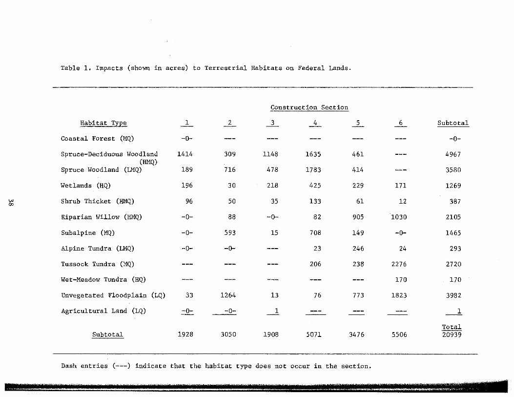
Table 1. Impacts (shown in acres) to Terrestrial Habitats on Federal Lands.
Construction Section
Habitat Type 2 5 6 Subtotal
Coastal Forest (MQ) -o- -0-
Spruce-Deciduous Woodland 1414 309 1148 1635 461 4967 (HMQ)
Spruce Woodland (LMQ) 189 716 478 1783 414 3580
Wetlands (HQ) 196 30 218 425 229 171 1269
w Shrub Thicket (HMQ) 96 50 35 133 61 12 387 co
Riparian Willow (HMQ) -0- 88 -0- 82 905 1030 2105
Subalpine (MQ) -0- 593 15 708 149 -0- 1465
Alpine Tundra (LMQ) -0- -0- 23 246 24 293
Tussock Tundra (MQ) 206 238 2276 2720
Wet-Meadow Tundra (HQ) 170 170
Unvegetated Floodplain (LQ) 33 1264 13 76 773 1823 3982
Agricultural Land (LQ) -0- -0- 1
Total Subtotal 1928 3050 1908 5071 3476 5506 20939
Dash entries (---) indicate that the habitat type does not occur in the section.
•11 1 i!!I!:SE!!!!!TJ!f! :rr:!!I T! .T !!!!!!!IJ!!·····r:r:!t!f.!!!?!! ! :r···:: ·· m:::::::::m;: sn .J ----
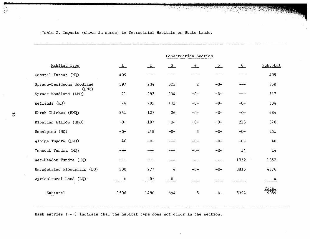
Table 2. Impacts (shown in acres) to Terrestrial Habitats on State Lands.
Construction Section
Habitat Type 1 2 4 5 6 Subtotal
Coastal Forest (MQ) 409 409
Spruce-Deciduous Woodland 397 234 325 2 -0- 958 (HMQ)
Spruce Woodland (LMQ) 21 292 234 -0- -0- 547
Wetlands (HQ) 24 205 105 -0- -0- -0- 334
w Shrub Thicket (HMQ) 331 127 26 -0- -0- -0- 484 \0
Riparian Willow (HMQ) -0- 107 -0- -0- -0- 213 320
Subalpine (MQ) -0- 248 -0- 3 -0- -0- 251
Alpine Tundra (LMQ) 40 -0- -0- -0- -0- 40
Tussock Tundra (MQ) -0- -0- 14 14
Wet-Meadow Tundra (HQ) 1352 1352
Unvegetated Floodplain (LQ) 280 277 4 -0- -0- 3815 4376
Agricultural Land (LQ) -0- 4
Total Subtotal 1506 1490 694 5 -0- 5394 9089
Dash entries (---) indicate that the habitat type does not occur in the section.
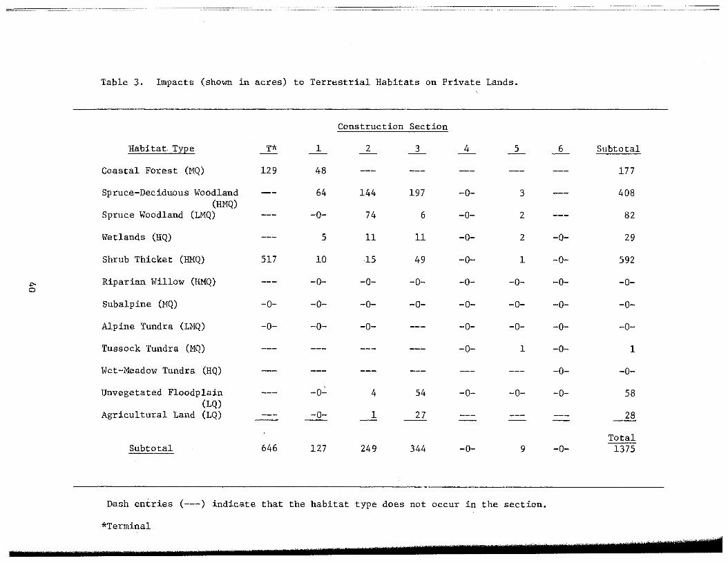
------~ .. ~---------···--·····--------------~----
Table 3. Impacts (shown in acres) to Terrestrial Habitats on Private Lands.
Construction Section
Habitat Type T* 3 4 6 Subtotal
Coastal Forest (MQ) 129 48 177
Spruce-Deciduous Woodland 64 144 197 -0- 3 408 (HMQ)
Spruce Woodland (LMQ) -0- 74 6 -0- 2 82
Wetlands (HQ) 5 11 11 -0- 2 -0- 29
Shrub Thicket (HMQ) 517 10 15 49 -o- 1 -0- 592
.p. Riparian Willow (HMQ) -0- -0- -0- -0- -0- -0- -0-0
Subalpine (MQ) -0- -0- -0- -0- -0- -0- -0- -0-
Alpine Tundra (LMQ) -0- -0- -0- -0- -0- -0- -0-
Tussock Tundra (MQ) -0- 1 -0- 1
Wet-Meadow Tundra (HQ) -0- -0-
Unvegetated Floodplain -a..:. 4 54 -0- -0- -0- 58 (LQ)
Agricultural Land (LQ) -0- 1 27 28
Total Subtotal 646 127 249 344 -0- 9 -0- 1375
Dash entries (---) indicate that the habitat type does not occur in the section.
1~Terminal

Table 4. Summary of Impacts (shown in acres) on Terrestrial Habitats by Land Ownership.
Habitat Type Federal Lands State Lands Private Lands Subtotal
Coastal Forest (MQ) -0- 409 177 586
Spruce-Deciduous Woodland (HMQ) 4967 958 408 6333
Spruce Woodland (LMQ) 3580 547 82 4209
Wetlands (HQ) 1269 334 29 1632
.j::-. Shrub Thicket (HMQ) 387 484 592 1463 1-'
Riparian Willow (HMQ) 2105 320 -0- 2425
Subalpine (MQ) 1465 251 -0- 1716
Alpine Tundra (LMQ) 293 40 -0- 333
Tussock Tundra (MQ) 2720 14 1 2735
Wet-Meadow Tundra (HQ) 170 1352 -0- 1522
Unvegetated Floodplain (LQ) 3982 4376 58 8416
Agricultural Land (LQ) 28 33
Total Subtotal 20939 9089 1375 31403
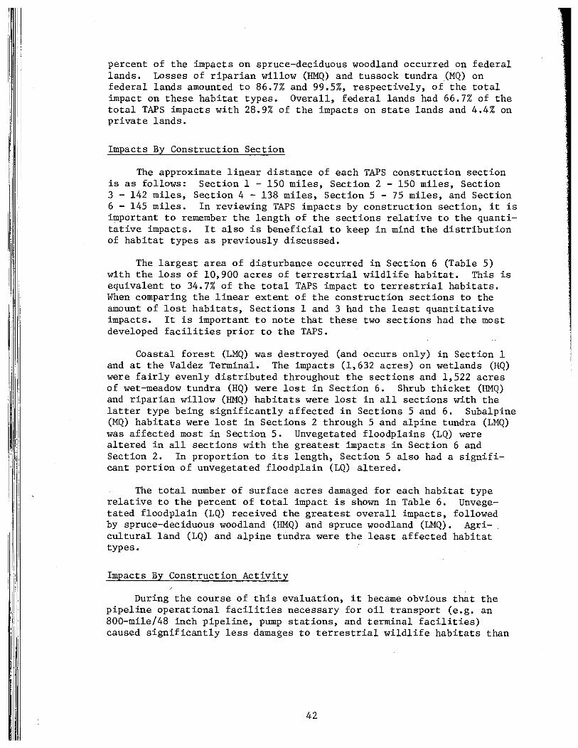
i :,
percent of the impacts on spruce-deciduous woodland occurred on federal lands. Losses of riparian willow (HMQ) and tussock tundra (MQ) on federal lands amounted to 86.7% and 99.5%, respectively, of the total impact on these habitat types. Overall, federal lands had 66.7% of the total TAPS impacts with 28.9% of the impacts on state lands and 4.4% on private lands.
Impacts By Construction Section
The approximate linear distance of each TAPS construction section is as follows: Section 1 - 150 miles, Section 2 - 150 miles, Section 3 - 142 miles, Section 4 - 138 miles, Section 5 - 75 miles, and Section 6 - 145 miles. In reviewing TAPS impacts by construction section, it is important to remember the length of the sections relative to the quantitative impacts. It also is beneficial to keep in mind the distribution of habitat types as previously discussed.
The largest area of disturbance occurred in Section 6 (Table 5) with the loss of 10,900 acres of terrestrial wildlife habitat. This is equivalent to 34.7% of the total TAPS impact to terrestrial habitats. When comparing the linear extent of the construction sections to the amount of lost habitats, Sections 1 and 3 had the least quantitative impacts. It is important to note that these two sections had the most developed facilities prior to the TAPS.
Coastal forest (LMQ) was destroyed (and occurs only) in Section 1 and at the Valdez Terminal. The impacts (1,632 acres) on wetlands (HQ) were fairly evenly distributed throughout the sections and 1,522 acres of wet-meadow tundra (HQ) were lost in Section 6. Shrub thicket (HMQ) and riparian willow (HMQ) habitats were lost in all sections with the latter type being significantly affected in Sections 5 and 6. Subalpine (MQ) habitats were lost in Sections 2 through 5 and alpine tundra (LMQ) was affected most in Section 5. Unvegetated floodplains (LQ) were altered in all sections with the greatest impacts in Section 6 and Section 2. In proportion to its length, Section 5 also had a significant portion of unvegetated floodplain (LQ) altered.
The total number of surface acres damaged for each habitat type relative to the percent of total impact is shown in Table 6. Unvegetated floodplain (LQ) received the greatest overall impacts, followed by spruce-deciduous woodland (HMQ) and spruce woodland (LMQ). Agricultural land (LQ) and alpine tundra were the least affected habitat types.
Impacts By Construction Activity
During the course of this evaluation, it became obvious that the pipeline operational facilities necessary for oil transport (e.g. an 800-mile/48 inch pipeline, pump stations, and terminal facilities) caused significantly less damages to terrestrial wildlife habitats than
42
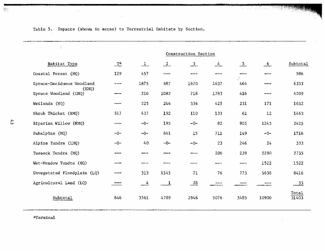
Table 5. Impacts (shown in acres) to Terrestrial Habitats by Section.
Construction Section
Habitat Type T* 1 2 3 4 5 6 Subtotal
Coastal Forest (MQ) 129 457 586
Spruce-Deciduous Woodland 1875 687 1670 1637 464 6333 (HMQ)
Spruce Woodland (LMQ) 210 1082 718 1783 416 4209
Wetlands (HQ) 225 246 334 425 231 171 1632
Shrub Thicket (HMQ) 517 437 192 110 133 62 12 1463
+:-Riparian Willow w (HMQ) -0- 195 -0- 82 905 1243 2425
Subalpine (MQ) -0- -0- 841 15 711 149 -0- 1716
Alpine Tundra (LMQ) -0- 40 -0- -0- 23 246 24 333
Tussock Tundra (MQ) 206 239 2290 2735
Wet-Meadow Tundra (HQ) 1522 1522
Unvegetated Floodplain (LQ) 313 1545 71 76 773 5638 8416
Agricultural Land (LQ) 4 1 33
Total Subtotal 646 3561 4789 2946 5076 3485 10900 31403
*Terminal
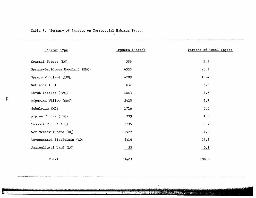
Table 6. Summary of Impacts on Terrestrial Habitat Types.
Habitat Type Impacts (Acres) Percent of Total Impact
Coastal Forest (MQ) 586 1.9
Spruce-Deciduous Woodland (HMQ) 6333 20.2
Spruce Woodland (LMQ) 4209 13.4
Wetlands (HQ) 1632 5.2
Shrub Thicket (HMQ) 1463 4.7
Riparian Willow (HMQ) 2425 7.7
Subalpine (MQ) 1716 5.5
Alpine Tundra (LMQ) 333 1.0
Tussock Tundra (MQ) 2735 8.7
Wet-Meadow Tundra (HQ) 1522 4.8
Unvegetated Floodplain (LQ) 8416 26.8
Agricultural Land (LQ) 33 0.1
Total 31403 100.0
the related activities (e.g. material sites, Haul Road, work pad, and access roads) associated with the construction effort. In order to determine those activities which had the most effects on terrestrial habitats, the impacts associated with pipeline operational facilities and construction-related facilities were analyzed. Impacts, categorized by construction activity for each section, are shown in Table 7. Percent of impacts by construction activity for each section are contained in Table 8 and a summary of construction-related impacts is shown in Table 9. Explanations of the various construction activities are contained in Appendix I.
The Haul Road (Plates 15, 16, & 17) was constructed in Sections 4, 5, and 6 and resulted in the permanent loss of 3,751 acres (Table 7) of terrestrial habitats. These impacts were caused not only from the areal extent of the gravel surfaces, but also from cut slopes, spoil areas adjacent to the road, and vehicle turn-outs built for rest areas. The length of the Haul Road through Section 4 is approximately 138 miles (1,432 acres damaged); Sections 5 and 6 are about 75 (841 acres) and 145 (1,478 acres) miles, respectively. Overall, each mile of the Haul Road directly destroyed about 10.5 acres of wildlife habitat.
Although the Yukon Highway (formally the TAPS Road) from Livengood to the Yukon River was not evaluated in this study, an estimate can be made of its impacts on terrestrial habitats. The Yukon Highway is about 56 miles long and was constructed in terrain that is similar to the southern portion of the Haul Road. Using the above figure of 10.5 acres of habitat damaged per mile of road, the Yukon Highway resulted in the loss of approximately 588 acres of terrestrial habitat. This figure does not include impacts associated with the material sites and other construction impacts of the Yukon Highway. Relative to the twelve habitat types used in this evaluation and the author's knowledge of the area, the most adversely affected habitats were spruce-deciduous woodland (HMQ) and spruce woodland (LMQ).
In Sections 1 through 4, the greatest impacts occurred from the construction of work pad (Plates 17- 21). Section 3 had 1,774 acres lost while Section 4 work pad impacts total 1,731 acres. The largest impacts to terrestrial habitats in Section 5 and 6 were caused by material sites which affected 1,268 and 6,528 acres, respectively (Plates 29 -34). In.Section 6, material site impacts were greater than the cumulative impact of all other construction activities.
Impacts resulting from access roads (Plates 21, 32, & 34) were relatively evenly distributed throughout the sections. Camps (~lates 25 & 26) and pump stations (Plates 27 & 28) resulted in the loss of 745 acres and 485 acres respectively. When surface impacts are complete for pump stations, the total loss of habitats from these permanent facilities will increase to an estimated 610 acres.
The impact figures for spur dikes (Plates 24 & 29) in Sections 5 and 6 are significantly less than the current actual losses since spur dike construction was not complete at the time of this evaluation.
45
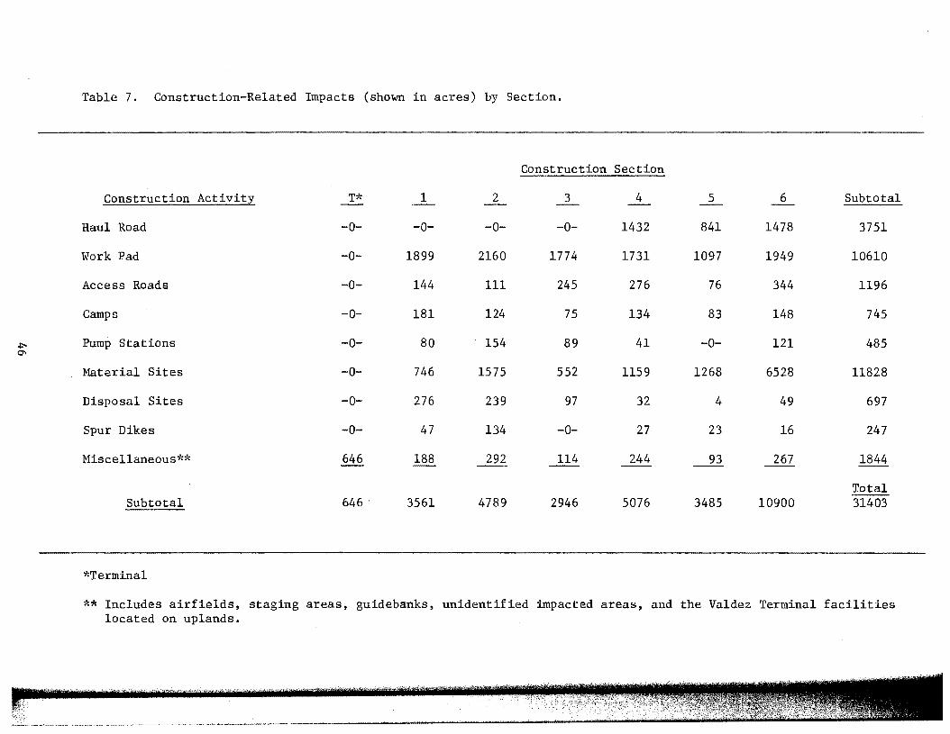
~ 0\
Table 7. Construction-Related Impacts (shown in acres) by Section.
Construction Section
Construction Activity T* 2 4 5 6 Subtotal
Haul Road -0- -0- -0- -0- 1432 841 1478 3751
Work Pad -0- 1899 2160 1774 1731 1097 1949 10610
Access Roads -0- 144 111 245 276 76 344 1196
Camps -0- 181 124 75 134 83 148 745
Pump Stations -0- 80 154 89 41 -0- 121 485
Material Sites -0- 746 1575 552 1159 1268 6528 11828
Disposal Sites -0- 276 239 97 32 4 49 697
Spur Dikes -0- 47 134 -0- 27 23 16 247
Miscellaneousi~* 646 188 292 114 244 267 1844
Total Subtotal 646. 3561 4789 2946 5076 3485 10900 31403
*Terminal
** Includes airfields, staging areas, guidebanks, unidentified impacted areas, and the Valdez Terminal facilities located on uplands.
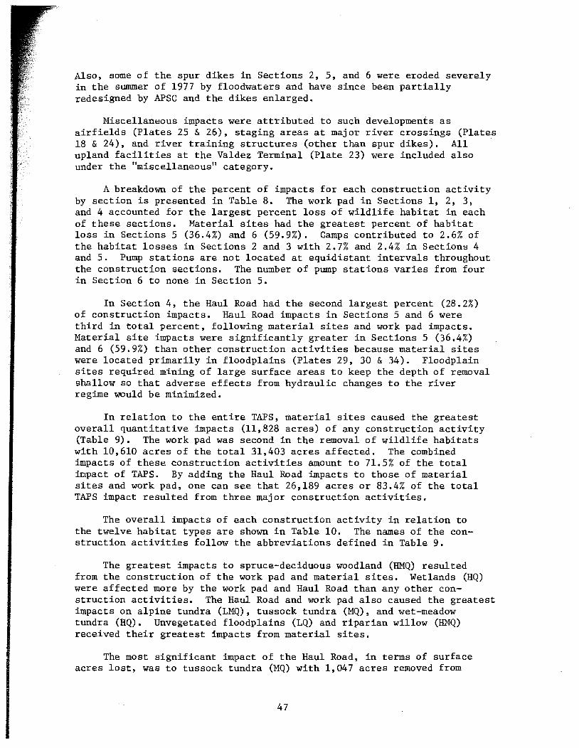
Also, some of the spur dikes in Sections 2, 5, and 6 were eroded severely in the summer of 1977 by floodwaters and have since been partially redesigned by APSC and the dikes enlarged.
Miscellaneous impacts were attributed to such developments as airfields (Plates 25 & 26), staging areas at major river crossings (Plates 18 & 24), and river training structures (other than spur dikes). All upland facilities at the Valdez Terminal (Plate 23) were included also under the "miscellaneous" category.
A breakdown of the percent of impacts for each construction activity by section is presented in Table 8. The work pad in Sections 1, 2, 3, and 4 accounted for the largest percent loss of wildlife habitat in each of these sections. Material sites had the greatest percent of habitat loss in Sections 5 (36.4%) and 6 (59.9%). Camps contributed to 2.6% of the habitat losses in Sections 2 and 3 with 2.7% and 2.4% in Sections 4 and 5. Pump stations are not located at equidistant intervals throughout the construction sections. The number of pump stations varies from four in Section 6 to none in Section 5.
In Section 4, the Haul Road had the second largest percent (28.2%) of construction impacts. Haul Road impacts in Sections 5 and 6 were third in total percent, following material sites and work pad impacts. Material site impacts were significantly greater in Sections 5 (36.4%) and 6 (59.9%) than other construction activities because material sites were located primarily in floodplains (Plates 29, 30 & 34). Floodplain sites required mining of large surface areas to keep the depth of removal shallow so that adverse effects from hydraulic changes to the river regime would be minimized.
In relation to the entire TAPS, material sites caused the greatest overall quantitative impacts (11,828 acres) of any construction activity (Table 9). The work pad was second in the removal of wildlife habitats with 10,610 acres of the total 31,403 acres affected. The combined impacts of these construction activities amount to 71.5% of the total impact of TAPS. By adding the Haul Road impacts to those of material sites and work pad, one can see that 26,189 acres or 83.4% of the total TAPS impact resulted from three major construction activities.
The overall impacts of each construction activity in relation to the twelve habitat types are shown in Table 10. The names of the construction activities follow the abbreviations defined in Table 9.
The greatest impacts to spruce-deciduous woodland (HMQ) resulted from the construction of the work pad and material sites. Wetlands (HQ) were affected more by the work pad and Haul Road than any other construction activities. The Haul Road and work pad also caused the greatest impacts on alpine tundra (LMQ), tussock tundra (MQ), and wet-meadow tundra (HQ). Unvegetated floodplains (LQ) and riparian willow (HMQ) received their greatest impacts from material sites.
The most significant impact of the Haul Road, in terms of surface acres lost, was to tussock tundra (MQ) with 1,047 acres removed from
47
~ ():)
Table 8. Percent (0.0%) of Construction-Related Impacts by Section.
Construction Section
Construction Activity T,'( 1 2 4 5 6
Haul Road o.o o.o 0.0 0.0 28.2 24.1 13.6
Work Pad o.o 53.3 45.1 60.2 34.1 31.5 17.9
Access Roads o.o 4.0 2.3 8.3 5.5 2.2 3.2
Camps o.o 5.1 2.6 2.6 2.7 2.4 1.4
Pump Stations o.o 2.2 3.2 3.0 0.8 0.0 1.1
Material Sites 0.0 21.0 32.9 18.7 22.8 36.4 59.9
Disposal Sites o.o 7.8 5.0 3.3 0.6 0.1 0.4
Spur Dikes o.o 1.3 2.8 0.0 0.5 0.6 0.1
Miscellaneous*ic 100.0 5.3 6.1 3.9 4.8 2.7
Total 100.0 100.0 100.0 100.0 100.0 100.0 100.0
*Terminal
**Includes airfields, staging areas, guidebanks, unidentified impacted areas, and the Valdez Terminal facilities located on uplands.
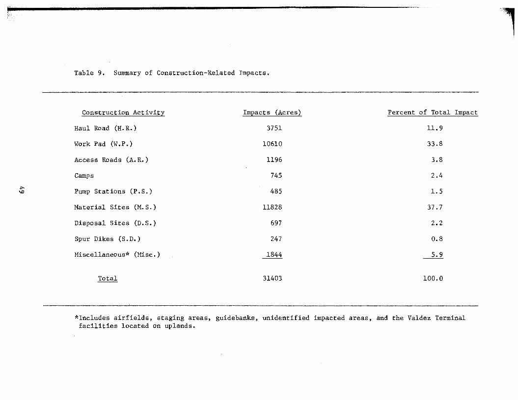
J::-. \0
Table 9. Summary of Construction-Related Impacts.
Construction Activit~ Impacts (Acres) Percent of Total Im:eact
Haul Road (H.R.) 3751 11.9
Work Pad (W .P.) 10610 33.8
Access Roads (A. R.) 1196 3.8
Camps 745 2.4
Pump Stations (P.S.) 485 1.5
Material Sites (M.S.) 11828 37.7
Disposal Sites (D.S.) 697 2.2
Spur Dikes (S.D.) 247 0.8
Miscellaneous* (Misc.) 1844 5.9
Total 31403 100.0
*Includes airfields, staging areas, guidebanks, unidentified impacted areas, and the Valdez Terminal facilities located on uplands.
.. .. ·1· .. ··.· ... · .
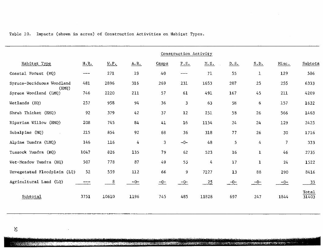
Table 10. Impacts (shown in acres) of Construction Activities on Habitat Types.
Habitat Type
Coastal Forest (MQ)
Spruce-Deciduous Woodland (HMQ)
Spruce Woodland (LMQ)
Wetlands (HQ)
Shrub Thicket (HMQ)
Riparian Willow (HMQ)
Subalpine (MQ)
Alpine Tundra (LMQ)
Tussock Tundra (MQ)
Wet-Meadow Tundra (HQ)
Unvegetated Floodplain
Agricultural Land
V1 0
Subtotal
(LQ)
(LQ)
H.R. W.P.
271
481 2896
746 2220
257 958
92 379
208 745
215 854
146 116
1047 826
507 778
52 559
8
3751 10610
Construction Activity
A.R. Camps P.S. M.S.
19 40 71
316 269 231 1653
211 57 61 491
94 36 3 63
42 37 12 251
84 41 16 1154
92 68 36 318
4 3 -o- 48
135 79 62 523
87 49 55 4
112 66 9 7227
-0- -0- -o- 25
1196 745 485 11828
D. S. S.D. Misc. Subtota
55 1 129 586
207 25 255 6333
167 45 211 4209
58 6 157 1632
58 26 566 1463
24 24 129 2425
77 26 30 1716
5 4 7 333
16 1 46 2735
17 1 24 1522
13 88 290 8416
-0- -0- 33
Total 697 247 1844 31403
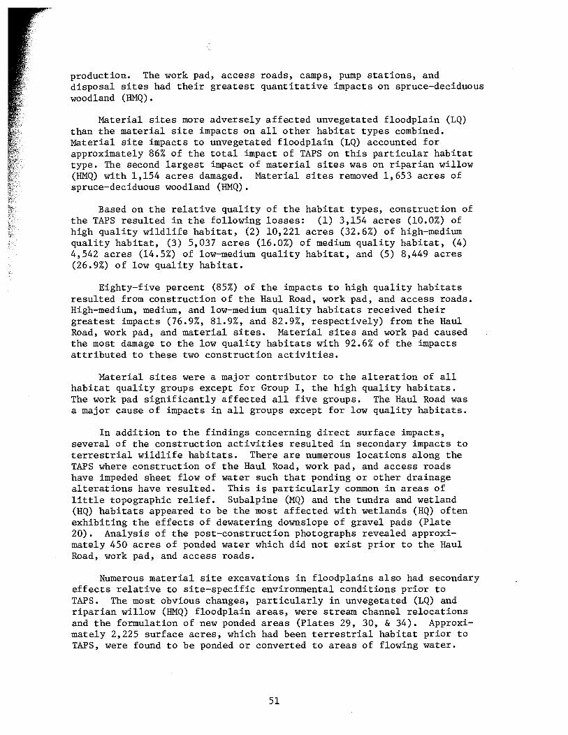
production. The work pad, access roads, camps, pump stations, and disposal sites had their greatest quantitative impacts on spruce-deciduous woodland (HMQ).
Material sites more adversely affected unvegetated floodplain (LQ) than the material site impacts on all other habitat types combined. Material site impacts to unvegetated floodplain (LQ) accounted for approximately 86% of the total impact of TAPS on this particular habitat type. The second largest impact of material sites was on riparian willow (HMQ) with 1,154 acres damaged. Material sites removed 1,653 acres of spruce-deciduous woodland (HMQ).
Based on the relative quality of the habitat types, construction of the TAPS resulted in the following losses: (1) 3,154 acres (10.0%) of high quality wildlife habitat, (2) 10,221 acres (32.6%) of high-medium quality habitat, (3) 5,037 acres (16.0%) of medium quality habitat, (4) 4,542 acres (14.5%) of low-medium quality habitat, and (5) 8,449 acres (26.9%) of low quality habitat.
Eighty-five percent (85%) of the impacts to high quality habitats resulted from construction of the Haul Road, work pad, and access roads. High-medium, medium, and low-medium quality habitats received their greatest impacts (76.9%, 81.9%, and 82.9%, respectively) from the Haul Road, work pad, and material sites. Material sites and work pad caused the most damage to the low quality habitats with 92.6% of the impacts attributed to these two construction activities.
Material sites were a major contributor to the alteration of all habitat quality groups except for Group I, the high quality habitats. The work pad significantly affected all five groups. The Haul Road was a major cause of impacts in all groups except for low quality habitats.
In addition to the findings concerning direct surface impacts, several of the construction activities resulted in secondary impacts to terrestrial wildlife habitats. There are numerous locations along the TAPS where construction of the Haul Road, work pad, and access roads have impeded sheet flow of water such that ponding or other drainage alterations have resulted. This is particularly common in areas of little topographic relief. Subalpine (MQ) and the tundra and wetland (HQ) habitats appeared to be the most affected with wetlands (HQ) often exhibiting the effects of dewatering downslope of gravel pads (Plate 20). Analysis of the post-construction photographs revealed approximately 450 acres of ponded water which did not exist prior to the_ Haul Road, work pad, and access roads.
Numerous material site excavations in floodplains also had secondary effects relative to site-specific environmental conditions prior to TAPS. The most obvious changes, particularly in unvegetated (LQ) and riparian willow (HMQ) floodplain areas, were stream channel relocations and the formulation of new ponded areas (Plates 29, 30, & 34). Approximately 2,225 surface acres, which had been terrestrial habitat prior to TAPS, were found to be ponded or converted to areas of flowing water.
51
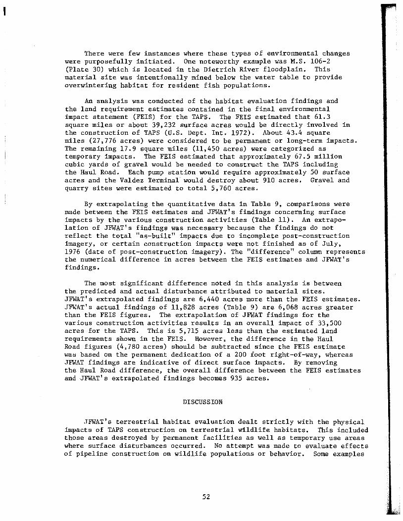
I
There were few instances where these types of environmental changes were purposefully initiated. One noteworthy example was M.S. 106-2 (Plate 30) which is located in the Dietrich River floodplain. This material site was intentionally mined below the water table to provide overwintering habitat for resident fish populations.
An analysis was conducted of the habitat evaluation findings and the land requirement estimates contained in the final environmental impact statement (FEIS) for the TAPS. The FEIS estimated that 61.3 square miles or about 39,232 surface acres would be directly involved in the construction of TAPS (U.S. Dept. Int. 1972). About 43.4 square miles (27,776 acres) were considered to be permanent or long-term impacts. The remaining 17.9 square miles (11,450 acres) were categorized as temporary impacts. The FEIS estimated that approximately 67.5 million cubic yards of gravel would be needed to construct the TAPS including the Haul Road. Each pump station would require approximately 50 surface acres and the Valdez Terminalwould destroy about 910 acres. Gravel and quarry sites were estimated to total 5,760 acres.
By extrapolating the quantitative data in Table 9, comparisons were made between the FEIS estimates and JFWAT's findings concerning surface impacts by the various construction activities (Table 11). An extrapolation of JFWAT's findings was necessary because the findings do not reflect the total "as-built" impacts due to incomplete post-construction imagery, or certain construction impacts were not finished as of July, 1976 (date of post-construction imagery). The "difference" column represents the numerical difference in acres between the FEIS estimates and JFWAT's findings.
The most significant difference noted in this analysis is between the predicted and actual disturbance attributed to material sites. JFWAT's extrapolated findings are 6,440 acres more than the FEIS estimates. JFWAT's actual findings of 11,828 acres (Table 9) are 6,068 acres greater than the FEIS figures. The extrapolation of JFWAT findings for the various construction activities results in an overall impact of 33,500 acres for the TAPS. This is 5,715 acres less than the estimated land requirements shown in the FEIS. However, the difference in the Haul Road figures (4,780 acres) should be subtracted since the FEIS estimate was based on the permanent dedication of a 200 foot right-of-way, whereas JFWAT findings are indicative of direct surface impacts. By removing the Haul Road difference, the overall difference between the FEIS estimates and JFWAT's extrapolated findings becomes 935 acres.
DISCUSSION
JFWAT's terrestrial habitat evaluation dealt strictly with the physical impacts of TAPS construction on terrestrial wildlife habitats. This included those areas destroyed by permanent facilities as well as temporary use areas where surface disturbances occurred. No attempt was made to evaluate effects of pipeline construction on wildlife populations or behavior. Some examples
52
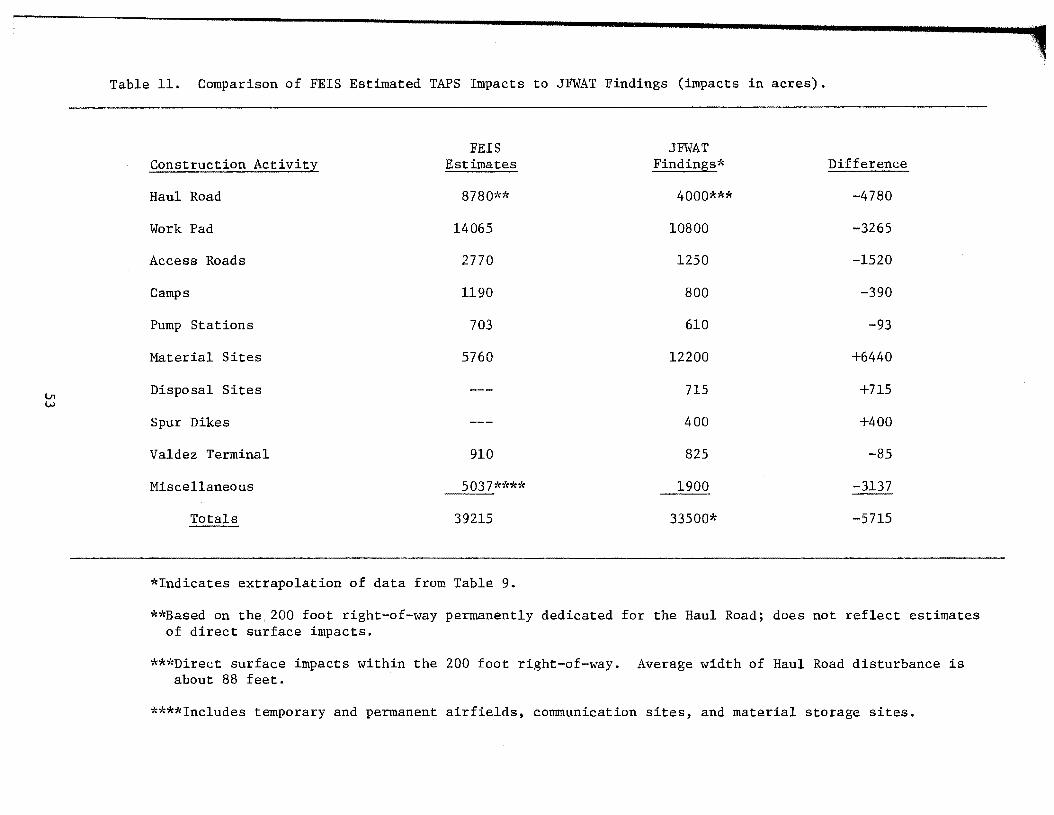
1..11 w
Table 11. Comparison of FEIS Estimated TAPS Impacts to JFWAT Findings (impacts in acres).
FEIS JFi.JAT Construction Activity Estimates Findings of~ Difference
Haul Road 8780** 4000*** -4780
Work Pad 14065 10800 -3265
Access Roads 2770 1250 -1520
Camps 1190 800 -390
Pump Stations 703 610 -93
Material Sites 5760 12200 +6440
Disposal Sites 715 +715
Spur Dikes 400 +400
Valdez Terminal 910 825 -85
Miscellaneous 5037*,~*1< 1900 -3137
Totals 39215 33500* -5715
*Indicates extrapolation of data from Table 9.
**Based on the 200 foot right-of-way permanently dedicated for the Haul Road; does not reflect estimates of direct surface impacts.
***Direct surface impacts within the 200 foot right-of-way. Average width of Haul Road disturbance is about 88 feet.
****Includes temporary and permanent airfields, communication sites, and material storage sites.
=>~I
!
of adverse effects of TAPS construction not covered in this evaluation include:
(1) noise, (2) dust, (3) harassment of wildlife (especially grizzly bears, Dall sheep,
moose, and caribou) by aircraft and vehicles, (4) blasting, (5) animal feeding (particularly bears, wolves, and foxes), (6) attraction of wildlife to camp refuse areas, (7) interruptions in normal migration and movement patterns, (8) illegal hunting, and (9) other human disturbances.
The impacts on wildlife habitats resulting from construction-related fuel spills, crude oil spills (Plate 13), man-caused thermal erosion (Plate 14), snow pads, and winter trails were not evaluated.
The TAPS construction section with the greatest overall impact on both federal and state lands was Section 6. Impacts on federal land in Section 6 totaled 5,506 acres (Table 1) while impacts on state lands were 5,394 acres (Table 2). The sum of these impacts (10,900 acres) is 34.7% of the total TAPS impact.
Over one-third of the total TAPS construction impacts occurred in an area which was slightly more than one-fifth of the total length of the TAPS corridor. The main reason this excessive amount of impact occurred in Section 6 was the number and size of material sites. A total of 6,528 surface acres (Table 7) of terrestrial wildlife habitat were altered significantly in order that material sources could be developed. This impact alone is quantitatively greater than the total impacts of any other construction section (Table 7).
The braided Sagavanirktok River was the primary gravel source in Section 6. Approximately 80% (5,200 acres) of the material site impacts were in unvegetated floodplains (LQ) with about 10% of the impacts occurring in riparian willow (HMQ) habitats. About one-fifth of the total surface disturbance of TAPS occurred in the Sagavanirktok River floodplain.
Section 3 had the least overall quantitative impacts (2,946 acres) of any construction section. This was due primarily to the number and location of existing facilities (e.g. the City of Fairbanks, roads, material sites, etc.) which were used by APSC during TAPS construction. Section 3 had the greatest percentage (8.3%) of access road damages to terrestrial habitats (Table 8). This was mainly a result of the relatively long access roads which had to be constructed from the Elliot and Yukon Highways to the TAPS' right-of-way.
54
Disposal sites in Sections 4, 5, and 6 had significantly less impacts on terrestrial habitats than the southern sections (Tables 7 and 8). There are several probable reasons for these differences:
(1) less need for disposal areas in the northern sections because of widespread tundra areas where clearing was minimal,
(2) the predominance of elevated pipe and reduced ditch spoil, and (3) mined-out areas of upland material sites used for disposal of
wastes in lieu of creating new disposal sites.
Construction camps ranged in size from about 25 acres to 50 acres. Camp airstrips and associated facilities varied in size from about 10 to 75 acres. Pump stations required between 38 and 55 acres per site.
The Haul Road was built in the northern sections for three main purposes:
(1) provide ground access for the logistical support of TAPS construction north of the Yukon River,
(2) provide easy access to the oil pipeline and related facilities during the operation and maintenance phase of the TAPS, and
(3) provide an overland transportation corridor to the Prudhoe Bay oil and gas fields and for futur~ developments.
As previously shown, construction of the Haul Road caused some of the most significant adverse impacts to high, high-medium, and medium quality wildlife habitats (Table 10). Continuing secondary impacts to wildlife habitats associated with the Haul Road include drainage alterations, aufeis, erosion, and fuel spills.
Future construction projects which require large amounts of gravel can be expected to cause significant widespread damages to terrestrial wildlife habitats which are part of major river floodplains, particularly in arctic regions. Secondary impacts resulting from hydrologic changes also can be anticipated. These statements are based on the following:
(1) either the gravel sources are located primarily in floodplain ~ areas, or
(2) the gravel sources are easily obtainable in the floodplain areas and approving officials concur with their exploitation in lieu of alternative sources.
Borrow materials (i.e. gravel, shotrock, etc.) from nearly 300 material sites were used to construct the Haul Road, work pad, access roads, spur dikes, camp pads, and other features of the TAPS. Burger and Swenson (1977) reported that approximately 61 million cubic yards of material had been extracted for TAPS construction purposes as of February, 1976. This information, coupled with the knowledge that approximately 11,828 acres of terrestrial habitat were altered to obtain this quantity of material, clearly indicates that siting of material sites is critical in minimizing unnecessary adverse impacts to wildlife habitats. This is
55
especially important when material sites are used during construction and throughout the operation phase of a project. Numerous TAPS material sites will be used during the operational phase for maintenance activities (e.g. Haul Road, work pad, and spur dikes).
Following material sites, the work pad damaged more wildlife habitat (10,610 acres) than any other construction activity (Table 9). The high quality habitat types incurred their greatest losses from construction of the work pad, followed by the Haul Road and then access roads (Table 10). High-medium and medium quality habitats also received some of their greatest impacts from the work pad and Haul Road. The impacts on wildlife habitats resulting from the Haul Road, work pad, and many of the access roads are permanent. Secondary effects (e.g. ponding, thermal erosion, and other drainage alterations) continue in some areas as a result of these construction activities.
During the timeframe in which the surface impacts of TAPS were calculated for this evaluation, restoration and revegetation efforts by APSC had been started but were minimal. The primary purpose of revegetation with grasses was to establish a ground cover as soon as possible to m1n1m1ze erosion. About 575 acres (Appendix II) had been revegetated with grasses (Plates 21 and 22) at the time of post-construction analysis. However, it was not until the summer of 1977 (oil began flowing through the pipeline in June, 1977) that comprehensive rehabilitation, restoration, and revegetation measures were implemented by APSC.
Various wildlife species have been observed feeding in revegetated areas (Plate 22). The overall habitat quality of areas revegetated with grasses is considered to be similar to agricultural land (i.e. low quality wildlife habitat) since it provides some food sources but satisfies few cover and reproduction requirements. APSC also attempted to reestablish woody shrubs, primarily alder (Alnus spp.) and willow (Salix spp.) in certain areas along the pipeline, but these efforts have been unsuccessful to date.
The most important element for minimizing long-term adverse impacts of gravel-pad construction (e.g. haul roads, access roads, and work pads) is the implementation of an inter-disciplinary evaluation of alignments and facility siting during the pre-construction phase of a project. This type of evaluation provides an opportunity to avoid loss of higher quality wildlife habitats when acceptable alternatives can be identified. It also allows for appropriate mitigative measures to be implemented regardless of the habitat quality. Once the alignment and facility locations are set and the structures built, the resulting impacts are usually permanent and irretrievable. As an example, Section 5 proposed access road alignments were field checked by a team consisting of:
(1) an APSC representative, (2) the construction contractor's representative, (3) an APO field engineer, and (4) a JFWAT biologist.
56
Proposed access routes were evaluated first for actual need and proximity to adjacent access roads. Following justification of a particular access road, its proposed alignment was scrutinized with respect to potential adverse environmental impacts and possible difficulties from a construction standpoint. In several instances, proposed access roads were moved to alternate locations or shifts made in the original alignments to avoid unnecessary loss of higher quality wildlife habitats.
Factors which play significant roles in the selection of material site locations are the availability of borrow materials that meet construction specifications, economics, potential difficulties associated with mining the materials, and environmental consequences. If severe impacts to wildlife habitats are to be minimized in future projects, it is imperative that proposed material site locations be evaluated by a process similar to that discussed above for roads and other projectrelated facilities.
Although the total FEIS estimate of surface requirements for TAPS was remarkably close to the total extrapolated figures of TAPS impacts determined by this study, the FEIS projection for surface impacts of material sites was extremely low (Table 11). This amplifies the importance of comprehensive, inter-disciplinary, pre-construction planning for future projects which require large amounts of gravel.
Both industry and government used the inter-disciplinary approach during the planning phase of the TAPS. This approach also was used to varying degrees during TAPS construction. There was, however, littie biological input into the alignment planning and construction of the Haul Road. TAPS impacts on wildlife habitats were quantitatively less than the FEIS predictions because of two basic reasons:
(1) government design review and field monitoring of TAPS construction on an inter-agency/inter-disciplinary basis and
(2) a generally comprehensive and enforceable set of stipulations designed to ensure pipeline integrity and protect environmental values.
Adverse impacts on wildlife habitats undoubtedly would have been greater had there not been government surveillance and enforcement of environmental and technical stipulations for construction and operation of the TAPS. There were many instances, during the construction of TAPS, where construction philosophies did not coincide with the best means for ensuring environmental protection. For example, most contractors wanted a normal work pad width for convenience at a small stream crossing rather than a "necked down" pad which would have decreased the destruction of riparian vegetation and minimize instream disturbances. Many contractors would have preferred to place overburden spoil from a newly opened floodplain material site into an adjacent wetland, stream channel, or floodplain rather than take the spoils to a mined-out, upland material site for disposal. The fact that sufficient erosion controls were not implemented, in many instances, until the summer of 1977 clearly indicates that environmental protection was oftentimes precluded by construction schedules.
57
•
The TAPS is an unprecedented "working model" of the environmental successes and failures of a major construction project in subarctic and arctic environments. Knowledge gained from TAPS is applicable to virtually all types of future construction projects. As time progresses, the longterm impacts and cumulative ramifications of TAPS on wildlife resources will become more apparent. Government and industry both have the responsibility and opportunity to work together to ensure that the expanding TAPS information base is used to benefit public wildlife resources which are threatened by the TAPS' operation phase, as well as future developments in the State of Alaska,
RECOMMENDATIONS
JFWAT's terrestrial habitat evaluation resulted in numerous recommendations, some are applicable to the TAPS' operational phase and others to future development projects in Alaska. Recommendations are separated into four categories.
1. General recommendations - possibly the most crucial for protecting wildlife resources threatened by major projects:
(a) During all phases of project development, an interagency/inter-disciplinary approach must be used to evaluate the potential adverse impacts of all project features on wildlife habitats. Examples of projects are: new facilities in the Prudhoe Bay oil and gas fields, oil development in the Kuparuk region, Susitna Hydroelectric Project, and the proposed Alaskan gas pipeline.
(b) Government agencies must ensure that comprehensive terrestrial (and aquatic) habitat evaluations of proposed project areas are conducted to identify wildlife (and fish) habitats in terms of quantity and quality.
(c) Emphasis must be placed on these evaluations during the preliminary planning and design stages prior to the construction phase.
(d) Results of inter-disciplinary evaluations must be incorporated into project designs to ensure the protection of wildlife habitats.
(e) Regardless of the habitat type, unnecessary and avoidable impacts must be eliminated.
(f) When adverse impacts are unavoidable, the least environmentally damaging alternative must be selected.
(g) Mitigative measures must be applied consistently throughout project development (e.g. alignment shifts, minimum pad widths, use of environmentally acceptable existing facilities, adequate cross drainage, proper waste disposal, and rehabilitation/restoration of disturbed areas).
58
(h) The project sponsor(s) should be required to adequately compensate for all significant unmitigated losses of public wildlife resources as determined by government resource agencies.
2. Recommendations for the TAPS' operational phase:
(a) Periodic government surveillance of TAPS and stipulation enforcement must continue to ensure the protection of project-affected wildlife resources.
(b) APSC's oil spill contingency plans, equipment, and procedures must be periodically reviewed and updated.
(c) APSC should continue to implement rehabilitation and restoration measures until natural vegetation communities have clearly reestablished on previously disturbed areas. Special attention should be given to restoring riparian willow (HMQ) and shrub thickets (HMQ), especially in Sections 5 and 6.
(d) Government resource agencies, in cooperation with APSC, should continue studies of the TAPS' revegetation program to determine what measures and procedures were successful for different site conditions. A detailed analysis of habitat regeneration should be conducted every fifth year (at a minimum) during the operation phase. This will assist in determining whether or not adequate rehabilitation is taking place.
(e) Resource agencies must work with the Alaska Department of Transportation (ADOT) and APSC to identify locations along the Haul Road and work pad where drainage alterations, caused by gravel pads, are affecting adversely terrestrial wildlife habitats (e.g. thermal erosion, aufeis, pending, and downslope dewatering of wetland communities). It is the responsibility of the land managing agencies to ensure that corrective actions for minimizing further damages are implemented in a timely manner.
(f) Resource agencies must conduct site-specific evaluations of the effects of gravel pads on wetlands (HQ), wetmeadow tundra (HQ), and associated biota. This is particularly important in areas of the Arctic Coastal Plain where oil and gas developments have increased significantly in the last five years.
(g) Abandoned access roads, camp pads, and airstrips should be used, whenever technically feasible, as material sources for maintenance operations in lieu of expanding or initiating new operational material sites.
59
l
1:
i
l:i
(h) Once operational material sites are depleted, they must be rehabilitated immediately. Revegetation measures must be applied by the end of the next growing season following the last use of the sites.
(i) If habitats damaged by TAPS construction and operation do not reestablish or major spills of crude oil severely affect wildlife habitats, compensation measures must be required of APSC to offset serious losses of wildlife resources.
3. Recommendations for future oil and gas pipelines:
(a) See 1 (a-h) above.
(b) Existing facilities, unless they have been found to be environmentally unsound, should be used to the greatest extent possible in lieu of damaging additional wildlife habitats. These decisions must be based on an interdisciplinary review of potential adverse effects of existing and proposed facilities.
(c) The potential for cumulative adverse impacts (e.g. effects of two parallel pipelines on caribou migrations, multiple drainage alterations, etc.) must be analyzed and appropriate actions taken to ensure that these impacts are minimized.
(d) The use of snow pads for construction of pipelines and resulting impacts on terrestrial wildlife habitats should be further researched.
(e) An inter-agency/inter-disciplinary surveillance organization must be implemented to review project designs, monitor project construction, and enforce environmental and technical stipulations so that impacts to wildlife habitats can be minimized throughout the project.
4. Recommendations for future, non-pipeline, development projects including roads, water-related projects, and mining:
(a) See 1 (a-h) above.
(b) Conduct terrestrial and aquatic habitat evaluations in preliminary planning stages for all sites being considered, including alternatives.
(c) Analyze proposed road alignments, material sites, and other development activities during planning, construction, and operation phases to identify temporary and permanent commitments of terrestrial wildlife habitats.
60
(d) Ensure that mitigative measures for unavoidable adverse impacts are incorporated into project designs and implemented during the construction, operation, and termination phases. Major development activities must be periodically monitored during operation so that unforeseen environmental impacts (e.g. drainage alterations and subsequent adverse effects on vegetation) can be corrected in a timely manner without unnecessary habitat losses for the project duration.
(e) Temporary-use facilities (e.g. construction camps, airfields, equipment storage areas) must be placed in environmentally sound locations which can be easily rehabilitated at completion of use. Recognize that temporary use of a habitat does not necessarily mean temporary disturbance. Some habitats are difficult, if not impossible, to restore (e.g. alpine tundra) and conventional measures may not be effective.
(f) Restoration and revegetation measures must be applied to disturbed areas as soon as construction or use of those areas is completed.
(g) Prior to construction, project sponsors should be required to post bonds which include assessments for potential damages to public wildlife resources. Funds for reestablishing wildlife habitats (both quantity and quality) also should be included.
SUMMARY
A classification system composed of twelve habitat types was used to cover type the 2,150 square mile study area. Habitat quality was determined by evaluating the food, cover, and reproduction requirements of 24 representative wildlife familites with respect to each habitat type. An LSD multiple range test was used to rank order the habitat types into five qualitative groups ranging from high to low quality habitats.
Construction of the 800-mile TAPS resulted in the loss of approximately 31,403 acres of terrestrial wildlife habitat. Impacts by land ownership were: 66.7% (20,939 acres) on federal lands, 28.9% (9,089 acres) on state lands, 4.4% (1,375 acres) on private lands. These overall percentages are not surprising since federal lands were involved for about two-thirds of the TAPS with slightly less than one-third of the distance being state lands.
Evaluation of the six construction sections indicated that the greatest quantitative impacts occurred in Section 6 with 10,900 acres of terrestrial habitats adversely affected by pipeline construction. This is about 34.7% of the total TAPS impact. Sections 1 and 3 had the least quantitative impacts (3,561 and 2,946 acres, respectively) which were expected since the southern sections had some developed facilities prior to TAPS construction.
61
Coastal forest was damaged (and occurs) only in Section 1 and at the Valdez Terminal. Spruce-deciduous woodland and spruce woodland were lost in all sections, except Section 6 where forest habitats do not exist. Alteration of wetlands, shrub thicket, riparian willow, and unvegetated floodplains occurred in all construction sections. Subalpine habitats were adversely affected in Sections 2 through 5 and alpine tundra was removed in Sections 1, and 4 through 6. Tussock tundra was lost in Sections 4 through 6 and wet-meadow tundra was removed in Section 6. Impacts to agricultural land occurred in the three southern sections.
The two habitat types rece1v1ng the greatest overall impacts were unvegetated floodplain and spruce-deciduous woodland. The least affected type was agricultural land.
The work pad, Haul Road, and access roads contributed the greatest impacts to high quality wildlife habitats. These impacts were both direct (destruction by gravel pads) and secondary (e.g. ponding and dewatering downslope).
Material sites damaged more terrestrial wildlife habitats (11,828 acres) than any other construction activity. The work pad caused the second greatest habitat loss (10,610 acres) with the Haul Road third in impacts (3,751 acres).
An extrapolation of JFWAT's quantitative findings to encompass all construction impacts resulted in an estimated 33,500 acres of terrestrial habitat damaged by the TAPS. This is 935 acres less than the FEIS prediction (not including the entire 200 foot Haul Road right-of-way) concerning the land requirements of TAPS. Government monitoring and enforcement by inter-agency/inter-disciplinary organizations and a comprehensive set of stipulations are probable reasons the quantitative impacts of TAPS were less than the FEIS predictions.
Recommendations for lessening impacts on terrestrial wildlife habitats are made that address the operational phase of TAPS and provide guidance for future development projects. Detailed inter-disciplinary reviews should be made of all proposed project features directly affecting land surfaces (e.g. roads, pipelines, other transportation alignments, material sites, construction camps, and other related facilities). During the early planning stages of a major project, habitat evaluations of alternative sites should be conducted to obtain an overall understanding of the quantity and quality of threatened wildlife resources. The least environmentally damaging alternative should be selected and appropriate mitigation and compensation measures incorporated into project designs.
62
REFERENCES
Alaska Dept. of Fish and Game. 1973. Alaska's wildlife and habitat. Anchorage, Alaska • 590 pp.
Anderson, M. 1973. Birds of Nuvagapak Point, northeastern Alaska. Arctic 26:186-197.
Bartonek, J.C. 1969. Arctic slope and trans-Alaska pipeline task force report: the bird resources of Alaska's arctic slope and petroleum development. North. Prairie Wildl. Res. Cen., Jamestown, N.D. 28 pp.
Bee, J.W. 1958. Birds found on the arctic slope of northern Alaska. Univ. Kansas, Mus. Nat. Hist. Publ. 10(5):163-211.
and E.R. Hall. 1956. Mammals of northern Alaska. Kansas, Mus. Nat. Hist. Misc. Publ. 8. 309 pp.
Bellrose, F.C. 1976. Ducks, geese and swans of North America. Books, Harrisburg, Pa. and Wildl. Mgmt. Inst., Wash. D.C.
Univ.
Stackpole 543 pp.
Bent, A.C. 1961. Life histories of North American birds of prey. Dover Publ., Inc., New York. 2 vols.
1962. Life histories of North American shore birds. Dover Publ., Inc., New York. 2 vols.
Bergman, R.D. 1974. Wetlands and waterbirds at Point Storkersen, Unpubl. Ph.D. Thesis, Iowa State Univ., Ames. 58 pp. Alaska.
----~~7., R.L. Howard, K.F. Abraham and M.W. Weller. 1977. Water birds and their wetland resources in relation to oil development at Storkersen Point, Alaska. U.S. Dept. Int., Fish & Wildl. Ser. Res. Publ. 129. 38 pp.
Brown, J. (ed.). 1975. Ecological and limnological reconnaissances from Prudhoe Bay into the Brooks Range, Alaska, summer, 1975. CRREL Res. Rep., Hanover, N.H. 65 pp.
1975. Ecological investigations of the tundra biome in the Prudhoe Bay region, Alaska. Univ. Alaska Biol. Pap. Spec. Rep. No. 2. 215 pp.
Cade, T.J. 1960. Ecology of the peregrine and gyrfalcon populations in Alaska. Univ. Calif. Publ. Zool. 63(3):151-290.
1967. Ecology of raptor populations in arctic Alaska. Submitted to the Arctic Inst. of N. Am. Rep. ONR Proj. 391.
1968. Ecology of raptor populations in arctic Alaska. Submitted to the Arctic Inst. of N. Am. Rep. ONR Proj. 409.
and R. Fyfe. 1970. The North American peregrine survey. Can. Field-Nat. 48:231-245.
63
Cameron, R.D. and K.R. Whitten. 1978. Third interim report of the effects of the trans-Alaska pipeline on caribou movements. Alaska Dept. of Fish and Game. Fed. Aid in Wild. Rest. Proj. W-17-9&10. Joint State/Federal Fish and Wildlife Advisory Team, Spec. Rep. No. 22. 29 pp.
Campbell, J.M. 1960. Nesting of the golden eagle in the central Brooks Range of arctic Alaska. Condor 62(4):298.
1969. The owls of the central Brooks Range, Alaska. Auk 86(3):565-568.
Chesemore, D.L. 1968. Distribution and movements of white foxes in northern and western Alaska. Can. J. Zool. 46:849-854.
1968. Notes on the food habits of arctic foxes in northern Alaska. Can. J. Zool. 46:1127-1130.
1969. Den ecology of the arctic fox in northern Alaska. Can. J. Zool. 47:121-129.
Cowan, I. MeT., W.S. Hoar and J. Hatter. 1950. The effect of forest succession upon the quantity and upon the nutritive values of woody plants used as food by moose. Can. J. Res. 28(D)(5):249-271.
Crook, J.L. 1971. Determination of abundance and distribution of brown bear (Ursus arctos) north of the Brooks Range, Alaska. Unpubl. M.S. Thesis, Univ. Alaska, College. 78 pp.
Dean, F.C. and D.L. Chesemore. 1975. Studies of birds and mammals in the Baird and Schwatka mountains, Alaska. Univ. Alaska Biol. Pap. No. 15. 80 pp.
Flood, B.S., M.E. Sangster, R.D. Sparrowe and T.S. Baskett. 1977. A handbook for habitat evaluation procedures. U.S. Dept. Int., Fish & Wildl. Ser. Res. Publ. 132. 77 pp.
Forest Management Institute. 1974. Vegetation types of the Mackenzie Corridor. Can. For. Ser., Envir. Can. Environmental Soc. Com., North. Pipelines, Task Force on North. Oil Devel. Rep. No. 73-46. 30 pp.
Fortenbery, D.K. 1974. Migratory birds, raptors, and endangered species. Resources Inventory, Arctic Planning Region. Joint Federal-State Land Use Planning Com. 34 pp.
Gabrielson, I.N. and F.C. Lincoln. 1959. Birds of Alaska. Stackpole Co., Harrisburg, Pa. and Wildl. Mgmt. Inst., Wash., D.C. 922 pp.
64
Gill, D. 1973. Ecological modifications caused by the removal of tree and shrub canopies in the Mackenzie Delta. Arctic 26(2):95-111.
Graber, J.W. and R.R. Graber. birds and their habitats. 97. 39 pp.
1976. Environmental evaluations using Ill. Nat. Hist. Sur. Biol. Notes No.
Grodzinski, W. 1971. Food consumption of small mammals in the Alaskan taiga forest. Ann. Zool. Fenn. 8:133-136.
Hall, R.H. and K.R. Kelson. 1959. The mammals of North America. Ronald Press Co., New York. 2 vols.
Hanson, H.C. 1953. Vegetation types in northwestern Alaska and comparisons with communities in other arctic regions. Ecology 34(1):111-140.
Hatler, D.F. 1972. Food habits of black bears in interior Alaska. Can. Field-Nat. 86:17-31.
Heimer, W.E. 1973. Dall sheep movements and mineral lick use. Alaska Dept. of Fish and Game. Fed. Aid in Wildl. Rest. Proj. W-17-2 through W-17-5. Juneau. 35 pp.
Hemming, J.E. 1971. The distribution and movement patterns of caribou in Alaska. Alaska Dept. of Fish and Game. Wildl. Tech. Bull. No. 1, Juneau. 60 pp •
• and K.A. Morehouse (ed.). 1976. Wildlife atlas: trans-----~~~-
Alaska oil pipeline, Valdez to Prudhoe Bay. Alaska Interagency Fish and Wildlife Team and the Joint State/Federal Fish and Wildlife Advisory Team. JS/FFWAT Spec. Rep. No. 3. 30 pp.
Hines, J.Q. 1963. Birds of the Noatak River, Alaska. Condor 65: 410-425.
Hjeljord, O.G. 1971. Feeding ecology and habitat preference of the mountain goat in Alaska. Unpubl. M.S. Thesis, Univ. Alaska, College. 126 pp.
Hobbie, J.E. and T.J. Cade, 1962. Observations on the breeding of golden eagles at Lake Peters in northern Alaska. Condor 64:235-237.
Holmes, R.T. and F.A. Pitelka. 1968. Food overlap among coexisting sandpip~rs on northern Alaska tundra. Syst. Zoo!. 17(3):305-318.
Hulten, E. 1968. Univ. Press.
Flora of Alaska and neighboring territories. 1,008 pp.
Stanford
Irvine, C.A. 1975. Black bear studies. Alaska Dept. of Fish and Game. Fed. Aid in Wildl. Rest. Proj. W-17-7, Juneau. 7 pp.
65
Irving, L. 1960. Birds of Anaktuvuk Pass, Kobuk, and Old Crow. U.S. Nat. Mus. Bull. 217. 409 pp.
Isleib, M.E. and B. Kessel. 1973. Birds of the North Gulf Coast -Prince William Sound region, Alaska. Univ. Alaska Biol. Pap. No. 14. 149 pp.
Johnson, P.L. and T.C. Vogel. 1966. Vegetation of the Yukon Flats Region, Alaska. CRREL Res. Rep. 209, Hanover, N.H. 53 pp.
King, J.G. 1970. The swans and geese of Alaska's arctic slope. Wildfowl 21:11-17.
and C.J. Lensink. 1971. An evaluation of Alaskan habitat migratory birds. U.S. Dept. Int., Bu. Sport Fish & Wildl.
Wash., D.C. 46 pp.
Kessel, B. and T.J. Cade. 1958. Birds of the Colville River, northern Alaska. Univ. Alaska Biol. Pap. No. 2. 83 pp.
and H.K. Springer. 1966. Recent data on status of some interior birds. Condor 68(2):185-195.
, R.B. Weeden and G.C. West. 1967. Bird- findings in interior and southcentral Alaska. Alaska Ornith. Soc. 42 pp.
Lensink, C.J., R.O. Skoog and J.L. Buckley. 1955. Food habits of marten in interior Alaska and their significance. J. Wildl. Mgmt. 37(3):364-368.
LeResche, R.E., R.H. Bishop and J.W. Coady. 1974. habitats of moose in Alaska. Naturaliste Can.
Distribution and 101:143-178.
MacLean, S.F., Jr., B.M. Fitzgerald and F.A. Pitelka~ 1974. Population cycles in arctic lemmings: winter reproduction and predation by weasels. Arctic Alpine Res. 6(1):1-12.
Manville, R.H. and S.P. Young. 1965. Distribution of Alaskan mammals. U.S. Dept. Int., Fish and Wildl. Serv., Cir. 211. 74 pp.
McGowan, J.D. 1975. Distribution, density and productivity of goshawks in interior Alaska. Alaska Dept. of Fish and Game. Fed. Aid in Wildl. Rest. Proj. W-17-3 through W-17-6, Job 10.6R. 31 pp.
Murie, A. 1944. The wolves of Mount Mckinley. U.S. Natl. Park Serv. Fauna Ser. No. 5. 238 pp.
_________ • 1962. Mammals of Mount Mckinley National Park, Alaska. Mount Mckinley Nat. Hist. Asso. 56 pp.
O'Farrell, T.P. 1965. interior Alaska.
Home range and ecology of snowshoe hares in J. Mammal. 46(3):406-418.
66
Pitelka, F.A. 1961. northern Alaska. Am. 18 pp.
Ecology of lemmings and other microtines in Rep. for 1960-61 submitted to Arctic Inst. of N.
1974. An avifaunal review for the Barrow region and north slope of arctic Alaska. Arctic Alpine Res. 6(2):161-184.
Rausch, R.A. Alaska.
1967. Some aspects of population ecology of wolves, Amer. Zool. 7(2):253-265.
Rausch, R.L. 1950. arctic Alaska •
Notes on microtine rodents from the Brooks Range, J. Wash. Acad. Sci. 40(4):133-136.
. 1951. Notes on the Nunamiut Eskimo and mammals of the ------:,-
Anaktuvuk Pass region, Brooks Range, Alaska. Arctic 4(3):148-195 •
• 1953. On the status of some arctic mammals. Arctic --6-::-(-:-:::2-:-) : 91-148.
Reeves, R.G., A. Anson, and D. Landen, eds. 1975. Manual of remote sensing. Amer. Soc. Photogrammetry, Falls Church, Virginia. 2 vols.
Reynolds, H.V. 1974. of Fish and Game. 25 pp.
North Slope grizzly bear studies. Alaska Dept. Fed. Aid in Wildl. Rest. Proj. W-17-6, Juneau.
Rutter, R.J. 1969. A contribution to the biology of the gray jay (Perisoeus canadensis). Can. Field-Nat. 83:300-316.
Sage, B.L. 1974. Ecological distribution of birds in the Atigun and Sagavanirktok River Valleys, arctic Alaska. Can. Field-Nat. 88:281-291.
Skoog, R.O. Alaska.
1968. Ecology of the caribou (Rangifer tarandus granti) in Unpubl. Ph. D. Thesis, Univ. Calif., Berkeley. 699 pp.
Special Habitat Evaluation Group. 1973. An inventory of wildlife habitat of the Mackenzie Valley and the northern Yukon. Can. Wildl. Ser., Dept. Envir. Environmental-Soc. Com., North. Pipelines, Task Force on North. Oil Devel. Rep. No. 73-27. 152 pp.
Spetzman, L.A. 1959. Vegetation of the arctic slope of Alaska. U.S. Dept. Int., Geol. Surv. Pap. 302-B. 39 pp.
Stephenson, R.O. 1971. Wolf report. Alaska Dept. of Fish and Game. Fed. Aid in Wildl. Rest. Proj. W-17-3, Juneau. 41 pp •
----,-• 1974. Characteristics of wolf den sites. Alaska Dept. of Fish and Game. Fed. Aid in Wildl. Rest. Proj. W-17-2 through W-17-6, Juneau. 27 pp.
Temple, S.A. Alaska.
1974. Winter food habits of ravens on the arctic slope of Arctic 27(1):41-46.
67
I
:I U.S. Department of Interior. 1972. proposed trans-Alaska pipeline. Wash., D.C.
Final environmental impact statement Government Printing Office.
U.S. Department of Interior. 1974. Agreement and grant of right-ofway for trans-Alaska pipeline between the United States of America and Amerada Hess Corp., ARGO Pipeline Co., Exxon Pipeline Co., Mobil Alaska Pipeline Co., Phillips Petroleum Co., Sohio Pipeline Co., and Union Alaska Pipeline Co. Government Printing Office. Wash., D.C.
U.S. Fish and Wildlife Service. 1976. Habitat evaluation procedures. U.S. Dept. Int., Fish & Wildl. Ser., Div. Ecol. Ser. Wash., D.C. 30 pp.
VanBallenberghe, V. 1978. Final report on the effects of the trans-Alaska pipeline on moose movements. Alaska Dept. of Fish and Game. Fed. Aid in Wildl. Rest. Proj. W-17-8. Joint State/Federal Fish and Wildlife Advisory Team, Spec. Rep. No. 23. 41 pp.
Viereck, L.A. and E.L. Little, Jr. U.S. Dept. Agri. Handbk. 410.
1972. Alaska trees and shrubs. 265 pp.
Wahrhaftig, C. 1965. Physiographic divisions of Alaska. U.S. Dept. Int., Geol. Surv. Pap. 482. 52 pp.
Weeden, R.B. 1965. Fish and Game. 110 pp.
Grouse and ptarmigan in Alaska. Fed. Aid in Wildl. Rest. Proj.
Alaska Dept. of W-6-R-5, Juneau
1969. Foods of rock and willow ptarmigan in central Alaska with comments on interspecific competition. Auk 86(2):271-281 .
------~-. and Lawrence N. Ellison. 1968. Upland game birds of forest
and tundra, Alaska Dept. of Fish and Game Wild!. Bkl. Series: No. 3, Juneau. 44 pp.
Welsh, S.L. 1974. Anderson's flora of Alaska and adjacent parts of Canada. Brigham Young Univ. Press, Provo, Utah. 724 pp.
Wiggins, I.L. and J.H. Thomas. 1962. A flora of the Alaskan arctic slope. Arctic Inst. N. Am. Spec. Publ. 4:3-31.
Wilimovsky, N.J. and J.N. Wolfe. 1966. Environment of the Cape Thompson Region, Alaska. U.S. Atomic Energy Com. 277-354.
Williamson, F.S.L. 1957. Ecological distribution of birds in the Napaskiak area of the Kuskokwim River Delta, Alaska. Condor 59:317-338 •
. and L.J. Peyton. 1962. ---------the Iliamna Lake area, Alaska. 73 pp.
Faunal relationships of birds in Univ. Alaska Biol. Pap. No. 5.
68
, , and M.E. Isleib. 1965. New distributional and ----------overwintering records of birds from southcentral Alaska. Condor 67(1):73-80.
White, C.M. and T.J. Cade. 1971. Cliff-nesting raptors and ravens along the Colville River in arctic Alaska. The Liv. Bird, Ten. Ann., 1971 Cornell Lab. Orni., Dec. 1, 1971. 107-150.
69
Appendix I: Glossary
70
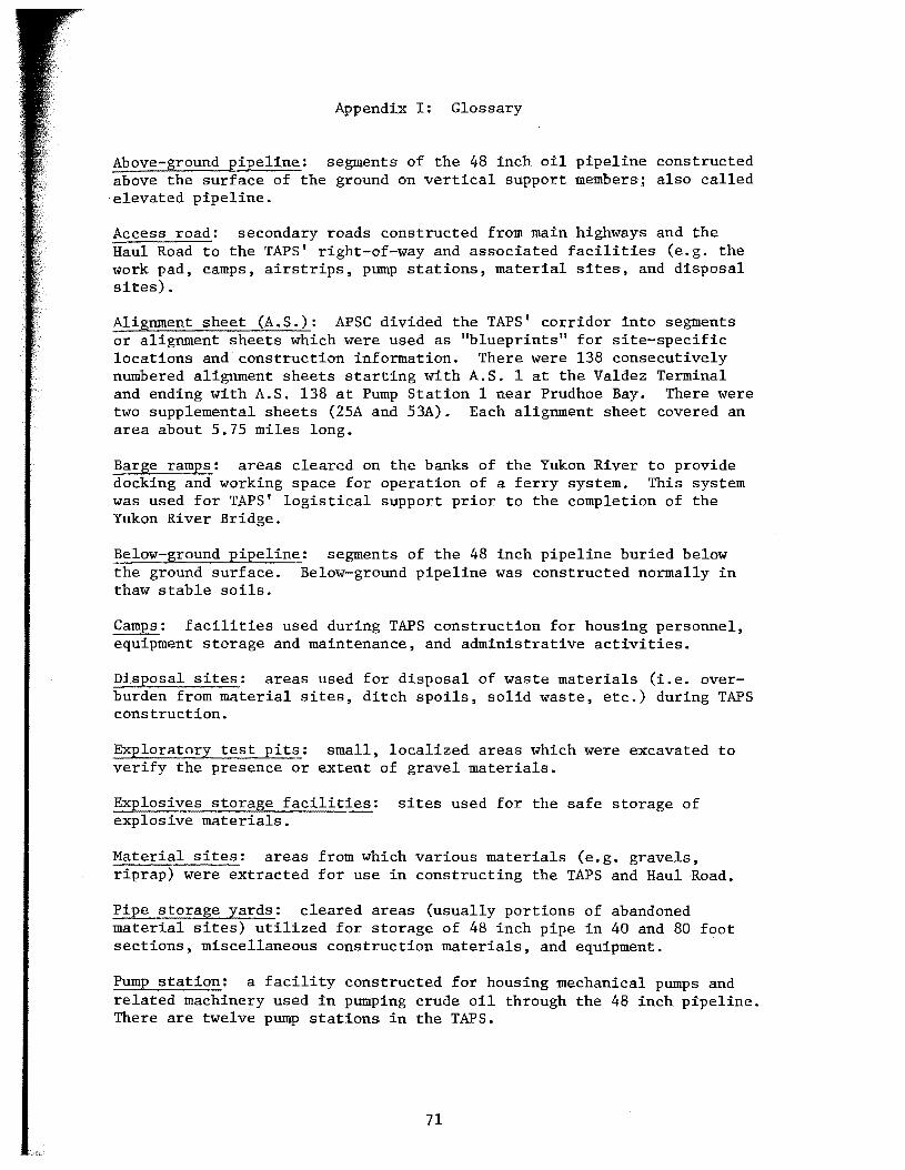
Appendix I: Glossary
Above-ground Eipeline: segments of the 48 inch oil pipeline constructed above the surface of the ground on vertical support members; also called
·elevated pipeline.
Access road: secondary roads constructed from main highways and the Haul Road to the TAPS' right-of-way and associated facilities (e.g. the work pad, camps, airstrips, pump stations, material sites, and disposal sites).
Alignment sheet (A.S.): APSC divided the TAPS' corridor into segments or alignment sheets which were used as 11blueprints" for site-specific locations and construction information. There were 138 consecutively numbered alignment sheets starting with A.S. 1 at the Valdez Terminal and ending with A.S. 138 at Pump Station 1 near Prudhoe Bay. There were two supplemental sheets (25A and 53A). Each alignment sheet covered an area about 5.75 miles long.
Barge ramps: areas cleared on the banks of the Yukon River to provide docking and working space for operation of a ferry system. This system was used for TAPS' logistical support prior to the completion of the Yukon River Bridge.
Below-ground pipeline: segments of the 48 inch pipeline buried below the ground surface. Below-ground pipeline was constructed normally in thaw stable soils.
Camps: facilities used during TAPS construction for housing personnel, equipment storage and maintenance, and administrative activities.
Disposal sites: areas used for disposal of waste materials (i.e. overburden from material sites, ditch spoils, solid waste, etc.) during TAPS construction.
Exploratory test pits: small, localized areas which were excavated to verify the presence or extent of gravel materials.
ExElosives storage facilities: sites used for the safe storage of explosive materials.
Material sites: areas from which various materials (e.g. gravels, riprap) were extracted for use in constructing the TAPS and Haul Road.
Pipe storage yards: cleared areas (usually portions of abandoned material sites) utilized for storage of 48 inch pipe in 40 and 80 foot sections, miscellaneous construction materials, and equipment.
PumE station: a facility constructed for housing mechanical pumps and related machinery used in pumping crude oil through the 48 inch pipeline. There are twelve pump stations in the TAPS.
71
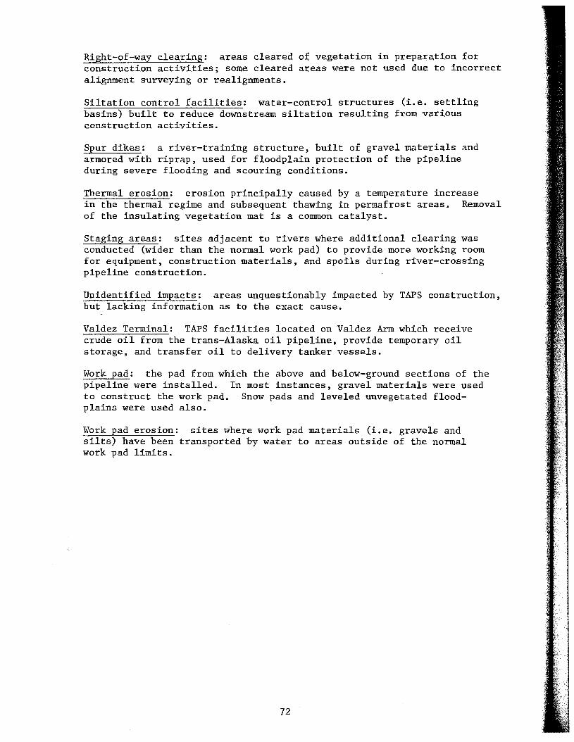
Right-of-way clearing: areas cleared o£ vegetation in preparation £or construction activities; some cleared areas were not used due to incorrect alignment surveying or realignments.
Siltation control facilities: water-control structures (i.e. settling basins) built to reduce downstream siltation resulting from various construction activities.
Spur dikes: a river-training structure, built of gravel materials and armored with riprap, used for floodplain protection of the pipeline during severe flooding and scouring conditions.
Thermal erosion: erosion principally caused by a temperature increase in the thermal regime and subsequent thawing in permafrost areas. Removal of the insulating vegetation mat is a common catalyst.
Staging areas: sites adjacent to rivers where additional clearing was conducted (wider than the normal work pad) to provide more working room for equipment, construction materials, and spoils during river-crossing pipeline construction.
Unidentified impacts: areas unquestionably impacted by TAPS construction, but lacking information as to the exact cause.
Valdez Terminal: TAPS facilities located on Valdez Arm which receive crude oil from the trans-Alaska oil pipeline, provide temporary oil storage, and transfer oil to delivery tanker vessels.
Work pad: the pad from which the above and below-ground sections of the pipeline were installed. In most instances, gravel materials were used to construct the work pad. Snow pads and leveled unvegetated floodplains were used also.
Work pad erosion: sites where work pad materials (i.e. gravels and silts) have been transported by water to areas outside of the normal work pad limits.
72
Appendix II: Pipeline ConstructionRelated Impacts
73
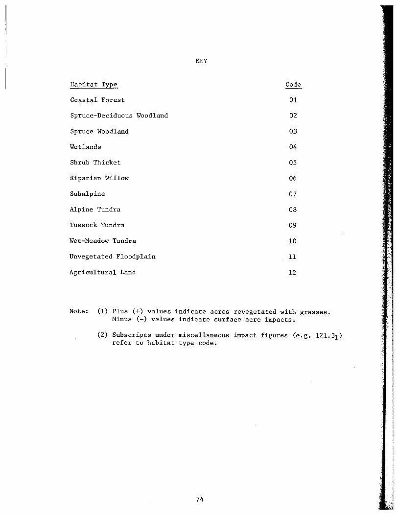
KEY
Habitat Type Code
Coastal Forest 01
Spruce-Deciduous Woodland 02
Spruce Woodland 03
Wetlands 04
Shrub Thicket 05
Riparian Willow 06
Subalpine 07
Alpine Tundra 08
Tussock Tundra 09
Wet-Meadow Tundra 10
Unvegetated Floodplain 11
Agricultural Land 12
Note: (1) Plus (+) values indicate acres revegetated with grasses. Minus (-) values indicate surface acre impacts.
(2) Subscripts under miscellaneous impact figures (e.g. 121.31) refer to habitat type code.
74
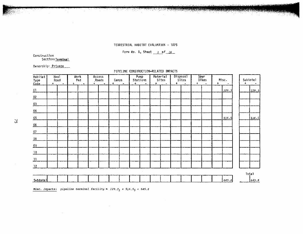
Construction Section:Terminal
Ownership: Private
Habitat Haul Type Road c'Orie + -01
02
03
04
05
06
07
08
09
10
11
12
_subtotal!
Work Access Pad .Roads
+ - +
TERRESTRIAL HABITAT EVALUATION - TAPS
Form No. 1, Sheet ___ l ___ Of__!§__
PIPELINE CONSTRUCTION-RELATED IMPACTS Pump Material Disposal
Camps Stations Sites Sites - + - + - + - + -
Misc. Impacts: pipeline terminal facility • 129.31 + 516.55 = 645.8
Spur Dikes Misc.
+ - + -129.3
516.5
1645.81
Subtotal + -
129.3
516.5
Total
'645.8
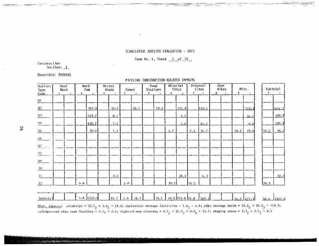
l rtmt~S IRJ At. 111\IH TJ\T EV/\I.UATION - TAPS
For-111 t!o. l,.Sheet Cou; trur lion
~ec t i 011: _!.....
PII'EI.INE CONSTI!UCTION-RELATED IMPACTS ------
Wor·k 14a ted a l Disposal Spur llob ita l Ita u l Access Pump Type l~oatl Pad Roads Camps Stat ions Sites Sitos Dikes Misc. J:.ili.l.c..... __ I· - + - + - -~ - ~- - + - + - + - i -·--'---·
Sul.ltota 1 + -
Ill ------ ··-- ·--· - --,__ ,_ -- - -- --- ----02 ----- .J.!!.J..:1. --..J!!..d. -- 2hL -- ...l2.:j_ 231.8 110.1 112. '\ 414
0:1 149.2 _Q_,J_ 5.2 - 14 4 -----· ----· ---- -- --- - 18~_:2
1)11 ---- ---· 168.2 7.1 --l..Jl.. 14 2 -O...ll. 195. t
()!) 30.6 1.1 1.7 2.3 34.7 16.5 29.8 20.5 96. ---- ----- ---------m.
1----, __ -___ , ___
--·--·-·-- -- ------ ----·----r--· --(J/ --- - ;--·" ·-. "~ ···---·· --- --- -- --
·--- ---- ---- -- ·---- ----·-(l') ---- --- -----.., ---- --· -- -- -----l 0_ -- ----·--·-------· -----'---- ------·---!1 __
1---- --- 0.2 . .1lhl 4.3 --- ----- -- -- ,...Jl..,l
lt. 4.6 1.0 39.2 33.5 78.3
!!:Jsc_,__.!!!!J~a_£Ul: airstrips"' 12.22
+ 3.65
15.8; <:!xploslves storage facill.ti<:!s = 1.62
= 1.6; pip<:! storage yards= 93.12 + 26.2 5 = 119.3;
r<:!t'rigerat<:!d pi.pe tust facility~ 2.l•z 2.1;; ri.ght-of-way clearlng = 0.72
·t-·32.23
+ 0.84 = 33.7; staging areas= 2.32 + 2.23 = 4.5
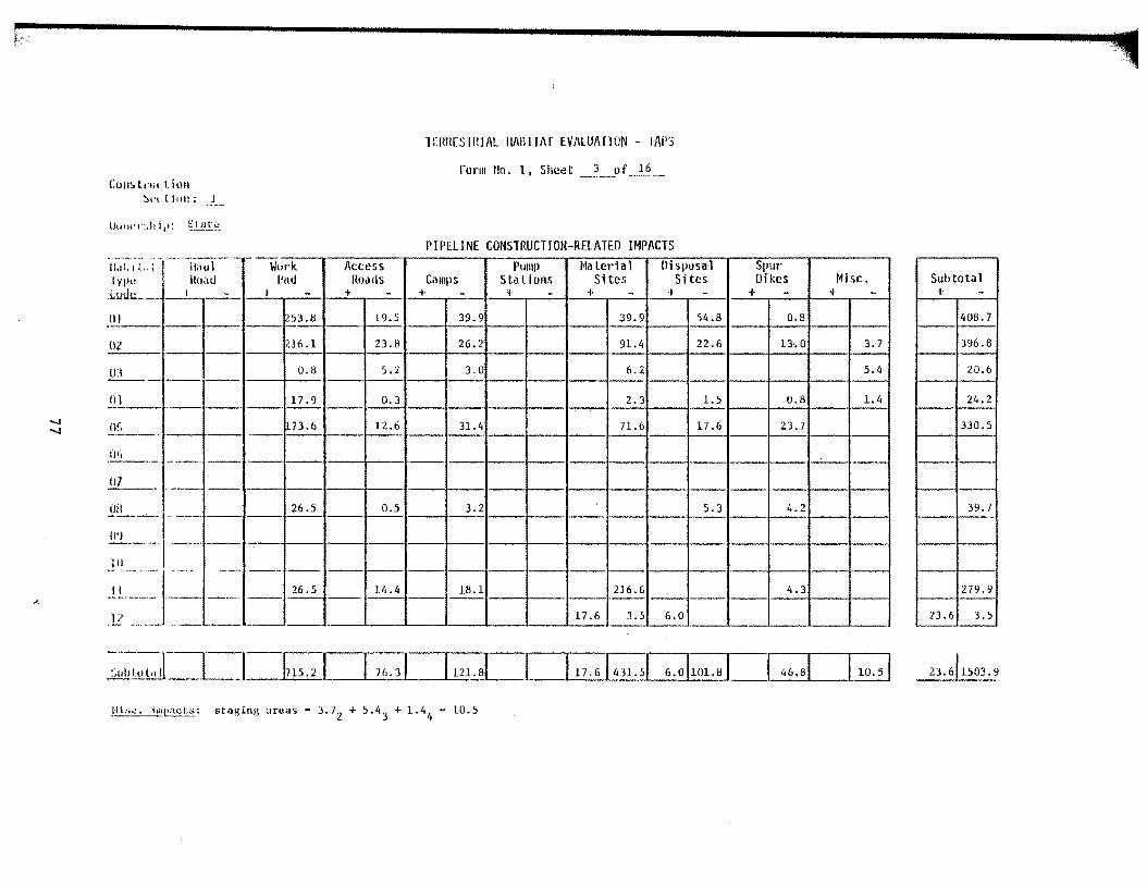
lrfm[SIItiAL IIABll'/\T EVI\lUi\TION - 11\P:i
rorm t!o. 1, Sheet 16 t:ou~ tnH1. ion
~i't I lnn; J
PIPELINE CONSTRUCTION-RELATED IMPACTS
U~d.1 L. \ lypt:
-~······ __ ..., ___ ._,_,,_
-Work lli.IU j Access PUIIII) 14a ter·i a 1 Disposal Spur-lto.1d Pad Roads Camps S ta lions SHes Sites Dikes Misc. Subtotal
Lulie. ___ ---'--- - I - + - + - 'I - + - + - + - i· - + -01 >53.1:! 19.5 39.9 39.9 54.8 0.8 408.7 ·-------- -- --· ~ ---- ----02 i2J6.1 23.8 26.2 91.4 22.6 n.o 3.7 --i---- 1·-
396.8 ·-
0:\ 0.8 5.2 3.0 6.2 5.4 20.6 --·-----.. --{).'} --- - 1:2.:2... 0.3 ~ 1.5 0.8 1.4
··-- --· --- 24.2
"'-l Wl "'-l ----- 73.6 12.6 31.4 71.6 17.6 23.7 ---- ----------·- - --·- 330.5
Ofi ·--·- --~----.. __ --- --
.Ql ___ ··--- -- -- -- - --
_Q_ll __ ~_ 26.5 0.5 3.2 5.3 4.2 ~·--·-· ----· -- ----- - ---- 39.7 ----
0'1 ----·· ----·· --~ -.. ...... _ .. --- --- ---- -----. ------------· r- --'---·
26.5 11!.!1 18.1 216.6 4.3 279.9 ·--- ----Wo• -- --- -- ----- -- - ---- --
17.6 3.5 6.0 23.6 3.5 .. ·---- ·-- -
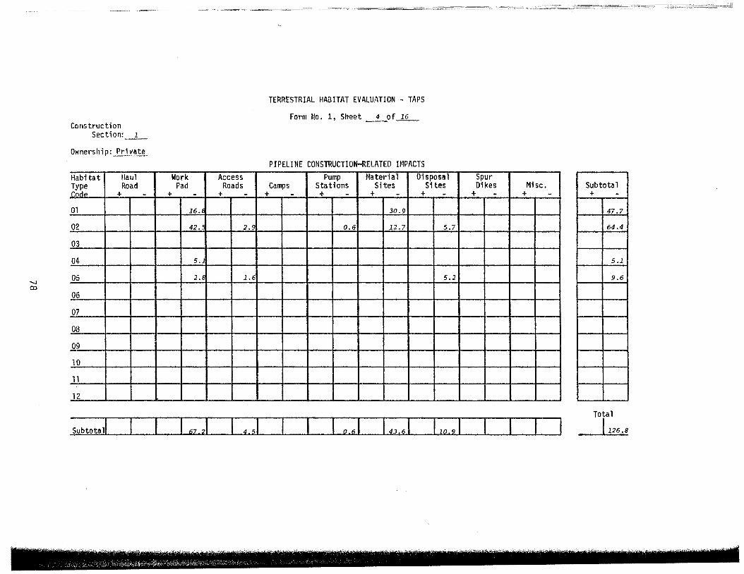
Construction Section: 1
Ownership: Private
Habitat Haul Type Road r.niiP + -01
02
03
04
05
06
07
08
09
10
11
12
Subtotal!
Work Access Pad Roads
+ - + -16.
42. 2.9
5.
2.6 1.6
67.21 4.51
TERRESTRIAL HABITAT EVALUATION - TAPS
Form No. 1, Sheet ___ 4 ___ of~
PIPELINE CONSTRUCTION-RELATED IMPACTS Pump Material Disposal
Camps Stations Sites Sites + - + - + - + -
30.9
0.6 12.7 5.7
5.2
143.61
Spur Dikes Misc.
+ - + - Subtota 1 + -
47.7
64.4
5.1
9.6
Total
1126.8
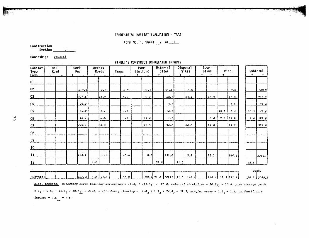
TERRESTRIAL HABITAT EVALUATION - TAPS
Form No. 1, Sheet _s_of ___,l,_L Consti"uctfon
Section 2
Ownership: Federal
PIPELINE CONSTRUCTION-RELATED IMPACTS Habitat Haul Work Access Pump Material IHsposal Spur
~!~: Road Pad Roads Camps Stations Sites Sites Dikes Mise. + - + - + - + - + - + - + - + - + -
Subtotal + -
01
02 219.9 7 .2 0.9 11 .2 53 .. 4 6 ~ Q.~ 1nR.R
03 497.6 1.4 5.6 39.7 60.7 63.4 19.9 17.9 716
04 25.2 3.3 1.1 29.6
05 30.9 1.7 1.6 14.2 30.3 1.4 30.3 49.8
06 42.7 0.6 1.3 14.4 1.5 3.4 7.0 23.9 7.0 ,;B'J.8
07 326.7 1.4 26.5 94.6 64.6 24.0 24.8 592.6
08
09
10
11 134.4 1.3 46.6 8.6 851.6 5.8 71.1 144.6 il2~4.n
12 6.2 31.6 11.0 48.8
Subtotal
Misc. impacts: accessory river training structures 11.46 + 113.611 = 125.0; material stockpiles = 10.811 = 10.8; pipe storage yards
9.62 + 6.5 3 + 12.56 + 12.611 = 41.2; right-of-way clearing= 11.43
+ 1.14
+ 24.87
= 37.3; staging areas 1.45
= 1.4; unidentifiable
impacts= 7.611
= 7.6
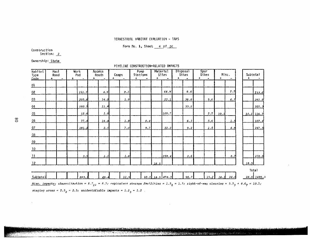
(X) 0
Construction Section: _]__
Ownership: State
Habitat Haul Type Road r.niiP +
01
02
03
04
05
06
07
08
09
10
11
12
Subtotal
- +
Work Access Pad Roads
- + -
151.7 4.9
205.€ 14.0
160. 11.4
12 .f. 1.9
77 -~ 14.0
191. 2.1
3.5 1.1
TERRESTRIAL HABITAT EVALUATION - TAPS
Form No. 1, Sheet __ 6_of ....l:.§..___
PIPELINE CONSTRUCTION-RELATED IMPACTS Pump Material Disposal
Camps Stations Sites Sites + - + - + - + -
0.2 64.9 9.4
1.9 22.1 36.0
33.2
109.7
1.8 0.4 6.3
7.0 9.7 22.2 9.2
1.6 259.4 2.6
18.5
Spur Dikes Misc.
+ - + -
2.5
5.6 6.
2.5 10.1
5.6 l.
1.5 4.
8.;
Subtotal + -
233.6
291.9
205.3
10 l 126.7
107.4
247.5
276.9
18.5
Total
28.611489.3
~isc. impact~ channelization 8.711 = 8.7; explosives storage facilities= 1.56 = 1.5; right-of-way clearing= 5.53 + 4.b7 = 10.1;
stagin'] areas= 2.52 = 2.5; unident.i:fiable impacts= 1.23 ;= 1.2.
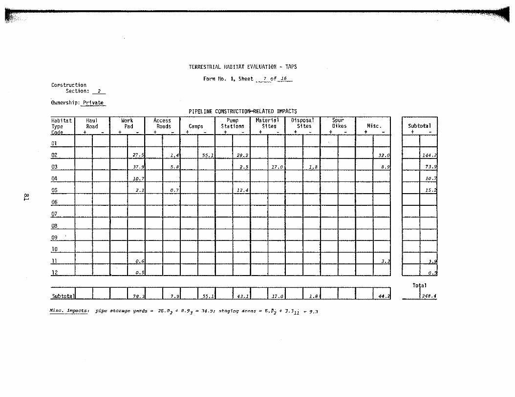
Construction Section: 2
Ownership: Private
Habitat Haul Type Road code + -01
02
03
04
05
06
07
08
09
10
11
12
Sub to tall
Work Access Pad Roads
+ - + -
27.5 1.4
37.9 5.8
10.7
2.1 0.7
0.6
0.5
I 79.J
TERRESTRIAL HABITAT EVALUATION - TAPS
Form No. 1, Sheet __ 7_of _l!L_
PIPELINE CONSTRUCTION-RELATED IMPACTS Pump Material Disposal
Camps Stations Sites Sites + - + - + - + -
55.1 28.2
2.5 17.0 1.8
12.4
:
55.11
Misc. impacts: pipe storage yards = 215.02 + 8.93 = 34.9; staging areas = 15.U2 + 3.311 = 9.3
Spur Dikes Misc. Subtotal
+ - + - + -
32.0 144.2
8.9 73.5
10.
15.
3.3 3.S
0.~
I 44.J
Torl 248.4
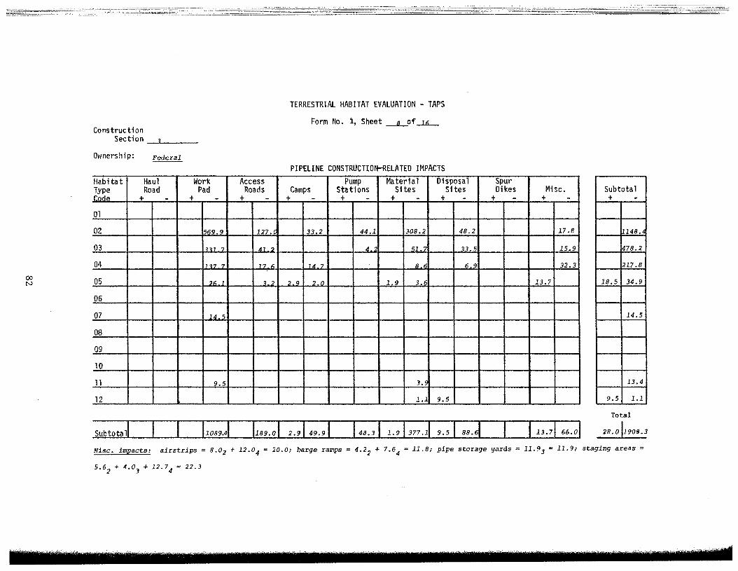
()::) N
TERRESTRIAL HABITAT EVALUATION - TAPS
Form No. 1, Sheet _LOf ....1.6........ Construction
Section _ _.__ __ _
Ownership: Federal
PIPELINE CONSTRUCTIOt+-RELATEO IMPACTS Habitat Haul Work Access Pump Material Disposal Spur
~~~: Road Pad Roads Camps Stations Sites Sites Dikes Misc. + - + - + - + - + - + - + - + - + -
Subtotal + -
01
02 'i69.9 127 .( 33.2 44.1 308.2 48.2 17.8 148.<
03 ln1 7 41.2 4 'il.7 33.5 15.9 478.2
04 '?7 7 17.6 14.7 8.6 6 9 32.3 217.8
05 :};; l ''L' 2.9 2.0 1.9 3.6 13.7 18.5 34.9
06
07 14 <; 14.5
08
09
10
11 9.5 3.5 13.4
12 1.1 9.5 9.5 1.1
Total
Subtotal 28.011908.3
Misc. impacts: airstrips= 8.02 + 12.04 ~ 20.0; barge ramps= 4.22 + 7.64 ~ 11.8; pipe storage yards= 11.93 = 11.9; staging areas
5.62 + 4.03 + 12.74 = 22.3
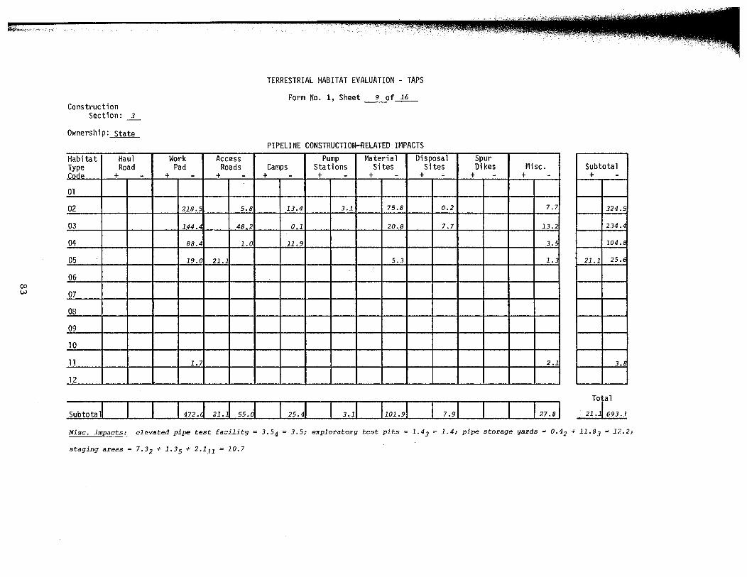
00 w
Construction Section: 3
Ownership: State
Habitat Haul Type Road code +
01
02
03
04
05
06
07
08
09
10
11
12
Subtotal!
- +
Work Access Pad Roads
- + - +
218.5 5.8
144.4 48.2
88.4 1.0
l9.C 21.1
1.7
1472.J nJ 55.J
TERRESTRIAL HABITAT EVALUATION - TAPS
Form No. 1, Sheet _9_of ...1§_
PIPELINE CONSTRUCTION-RELATED IMPACTS Pump Material Disposal
Camps Stations Sites Sites - + - + - + -
13.4 3.1 75.8 0.2
0.1 20.8 7.7 11.9
5.3
Spur Dikes Misc.
+ - + -
7.7 13.
3.5
l.
2.1
127.81
Subtotal + -
324.5
234.4
104.8
21.1 25.6
3.8
Total
21.1,693.1
Misc. impacts: elevated pipe test facility = 3.54 = 3.5; exploratory test pits= 1.43 = 1.4; pipe storage yards = 0.42 + 11.83 = 12.2;
staging areas= 7.32 + 1.35 + 2.111 = 10.7
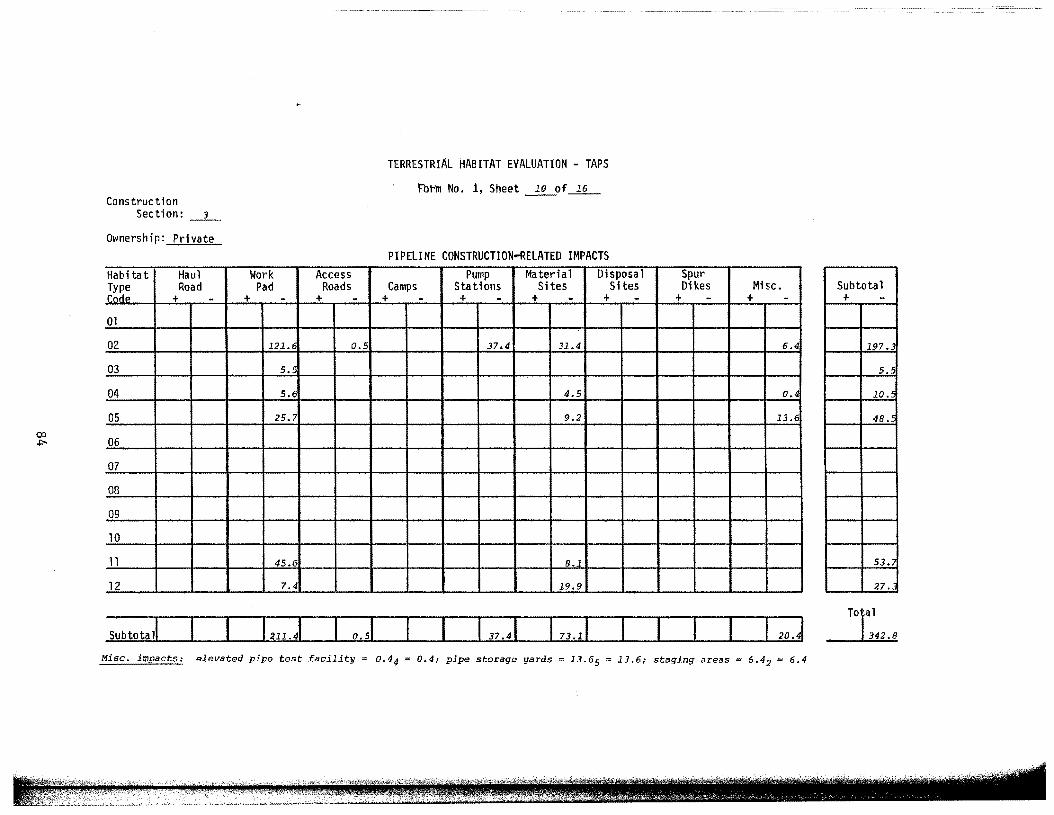
Construction Section: _3_
Ownership: Private
Habitat Haul
~~~; Road + -
01
02
03
04
05
06
07
08
09
10
11
12
Subtotal!
Work Access Pad Roads
+ - + - +
121.6 0.5
5 • .5
5.6
25.7
45.6
7.4
o.sl
TERRESTRIAL HABITAT EVALUATION - TAPS
tbrm No. 1, Sheet ___EL_of _1§__
PIPELINE CONSTRUCTION~ELATED IMPACTS Pump Material Disposal Spur
Camps Stations Sites Sites Dikes Misc. - + - + - + - + - + -
37.4 31.4 6.4
4.5 0.4
9.2 13.6
8.1
19.9
I 20.J
Misc. impacts: elevated pipe test facility 0.44 0.4; pipe storage yards= 13.65 = 13.6; staging areas = 6.42 = 6.4
Subtotal + -
197.
s.~
10.
48.
53.
27.
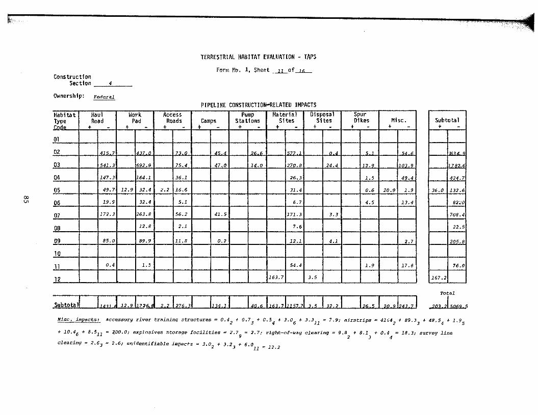
TERRESTRIAL HABITAT EVALUATION - TAPS
Form ~!o. 1, Sheet ___,U__.Of __.1_6__
Construction Section __ 4.:_.. __
Ownership: Federal
PIPELINE CONSTRUCTION-RELATED IMPACTS Habitat Haul Work. Access Pump Material Disposal Spur
~~~= Road Pad Roads Camps Stations Sites Sites Dikes Misc. + - + - + - + - + - + - + - + - + -
Subtota 1 + -
01
02 415 7 !4~7 .0 73.0 45.4 26.6 1577.1 0 4 ~ I ~tJ " II>~ 4 <l
03 541.3 692.9 75.4 47.0 14.0 270.8 24.4 12.9 103.9 h 7 82.6
04 147.3 164.1 36.1 26.3 1.5 49.4 424.7
05 49.7 12.9 32.4 2.2 16.6 31.4 0.6 20.9 1.9 36.0 132.6
06 19.9 32.4 5.1 6.7 4.5 13.4 82;.!0
07 172.3 263.8 56.2 41.5 171.3 3.3 708.4
08 12.8 2.1 7.6 22.5
09 85.0 89.9 11.8 0.2 12.1 4.1 2.7 205.8
10
11 0.4 1.5 54.4 1.9 17.8 76.0
12 163.7 3.5 167.2
Subtotal! 11411 J 12.911726.J 2.21276.A L6.5 120.912~3.71 Total
2Ql 215Q.69. 5
Misc. impacts: accessory river training structures= 0.42 + 0.73
+ 0.54
+ 3.06
+ 3.311
= 7.9; airstrips= 41142
+ 89.33
+ 48.54
+ 1.95
+ 10.46 + 8.511 = ~00.0; explosives storage facilities = 2.7 = 2.7; right-of-wag clearing = 9.8 + 8.1 + 0.4 = 18.3; survey line 9 2 3 4
clearing = 2.63 = 2.6; unidentifiable impacts 3 0 + 3 2 + 6 0 • 2 • 3 • 11 = 12.2
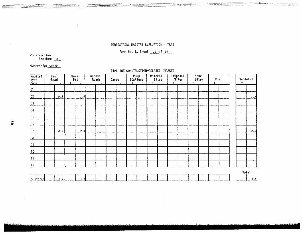
Construction Section: _4_
Ownership: State
Habitat Haul Type Road code + -Ol
02 0.3
03
04
05
06
07 0.4
08
09
10
11
12
Subtota 1!
Work Access Pad Roads
+ - + -
1.<
2.4
I 3.J
TERRESTRIAL HABITAT EVALUATION - TAPS
Form No. 1, Sheet _E_of ...1.§._
PIPELINE CONSTRUCTION-RELATED IMPACTS Pump Material Disposal Spur
Camps Stations Sites Sites Dikes Misc. Subtotal + - + - + - + - + - + - + -
1 7
2.8
Total
I 4.5
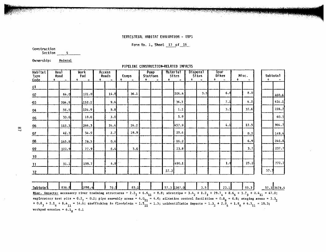
Construction Section----='----
Ownership: Federal
Habitat Haul Work Type Road Pad coite + - + -01
02 64.C 121.0
-()J 204.9 152.2
04 56.9 124.9
05 33.6 18.0
06 115.3 266.3
07 42.3 54.9
08 145.8 76.5
09 122. s 77.9
10
l1 51. 199.7
12
Subtotal
Access Roads
+ - +
14.8
9.6
9.8
3.0
24.4
2.7
0.6
6.4
4.8
TERRESTRIAl HABITAT EVALUATION - TAP$
Form flo. 1, Sheet ~of~
PIPELINE CONSTRUCTION-RELATED IMPACTS Pump Material Ofsposal Spur
Camps Stations Sftes Sites Dikes Mfsc. Subtotal - + - + - + - + - + - + -
36.1 206.4 3.5 6.f 8.0 460.6
36.1 7. 4.2 414.1
1.2 3. 32.6 228.7
5.9 60.5
24.2 457.9 4. 12.5 904.7
19.9 29.4 0,2 149.4
16.2 6.9 246.0
3.0 23.8 3.7 237.7
490.1 1. 25.2 772.7
57.3 57.
Misc. impacts: accessory river training structures= 2.23 + 6.611 = 8.8; airstrips= 3.42 + 1.23 + 29.74
+ 8.66 + 3.79
+ 0.411 = 47.0;
exploratory test pits = 0.27 = 0.2; pipe assembly areas = 4.o11 4.0; siltation control facilities = 0.88 = 0.8; staging areas = 3.32 + 0.83 + 2.1
6 + 8.4
11 = 14.6; trafficking in floodplain= 1.5
11 1.5; unidentifiable impacts= 1.3
2 + 2.9
4 + 1.8
6 + 4.311 = 10.3;
workpad erosion = 6.18
= 6.1
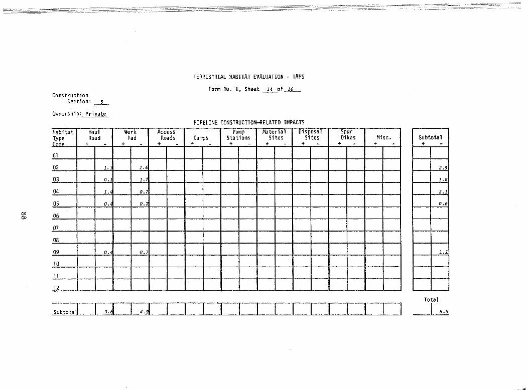
Construction Section: _s_
Ownership: Private
Habitat Haul Type Road CodP. + -01
02 1.
03 o.
04 1.
05 o.
06
07
08
09 o.
10
11
12
Subtotal! I 3.J
Work Access Pad Roads
+ - + -
1.6
1.
0.7
0.2
0.7
TERRESTRIAL HABITAT EVALUATION - TAPS
Form No. 1, Shee.t ___!!__of ...1.§._
PIPELINE CONSTRUCTION-RELATED IMPACTS Pump Material Disposal Spur
Camps Stations Sites Sites Dikes Misc. Subtotal + - + - + - + - + - + - + -
2.9
l.B
2.1
0.6
l.l
Total
I 8.5
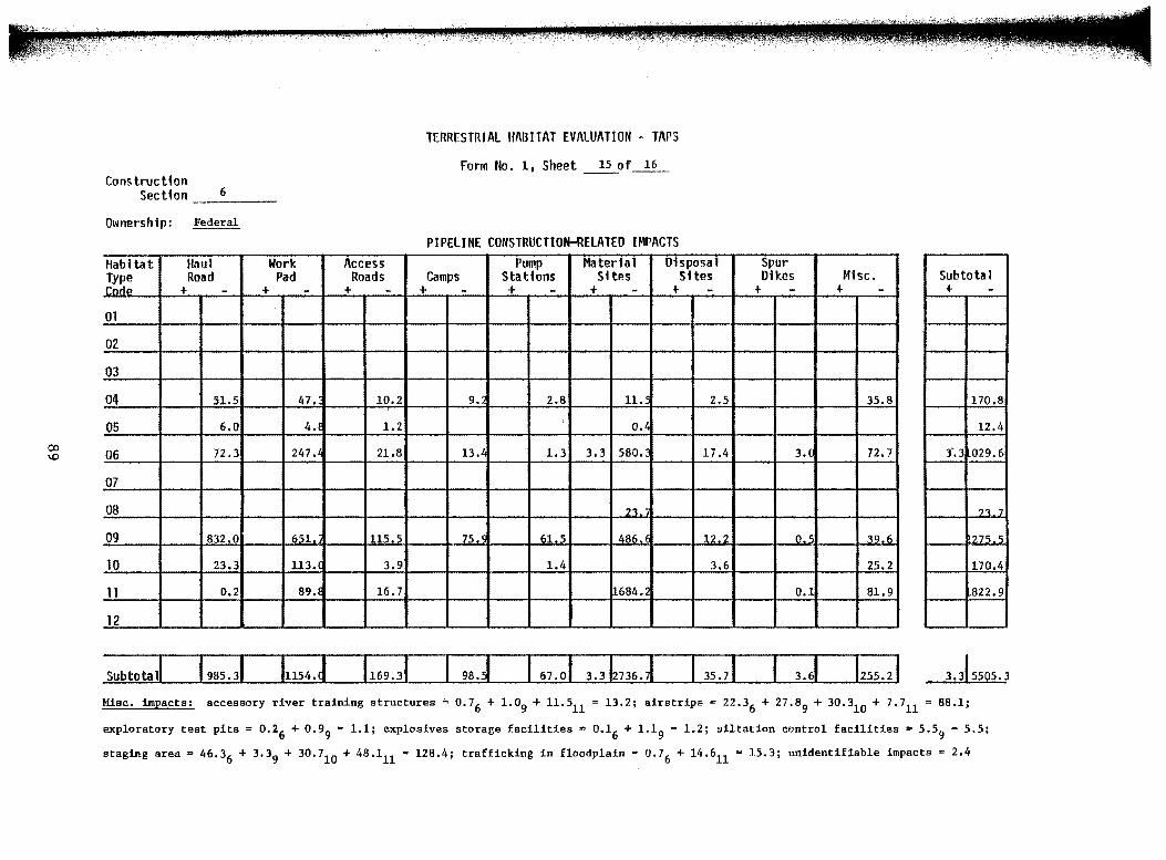
TERRESTRIAL HABITAT EV/\LUATION - TAPS
Form No. 1, Sheet ~of~ Construction
Section __ 6 __ _
Ownership: Federal
PIPELINE CONSTRUCTION-RELATED IMPACTS Habitat Haul Work Access Pump Material Disposal Spur Type Road Pad Roads Camps Stations Sites Sites Dikes Misc. code + - + - + - + - + - + - + - + - + -
Subtotal + -
01
02
03
04 51.5 47. 10.2 9. 2.8 11. 2.5 35.8 170.8
05 6.0 4.! 1.2 ' o.~ 12.4
06 72.3 247 ,l 21.8 l3,l 1.3 3.3 580. 17.4 3.0 72.7 3-.3 029.6
07
08 23 2'L7
09 832.0 651. 1155 75.9 615 486.t 12 2 0 5 39.6 t275 5
10 23.3 113.( 3.9 1.4 3.6 25.2 170.4
11 0.2 89.! 16.7 684.£ 0.1 81.9 822.9
12
Subtotal 3.3,5505.3
Misc.. impacts: accessory river training structures z 0.76 + 1.09 + 11.511 = 13.2; airstrips= 22.36 + 27.89
+ 30.310 + 7.711 = 88.1;
exploratory test pits = 0.26 + 0.99 = 1.1; explosives storage facilities = 0.16 + 1.19 = 1.2; siltation control facilities = 5.59 = 5.5;
staging area= 46.36 + 3.39 + 30.710 + 48.111 = 128.4; trafficking in floodplain = 0.76 + 14.611 = 15.3; unidentifiable impacts = 2,4
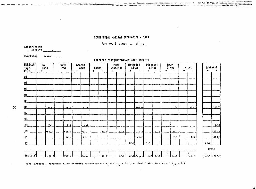
TERRESTRIAL HABITAT EVALUATION - TAPS
Form flo. 1, Sheet ....l.li.-of ....1.6...._ Construction
Section __ __.... __
Ownership: State
PIPELINE CONSTRUCTION-RELATED IMPACTS Habitat Haul Work Access Pump Material Disposal Spur Type Road Pad Roads Camps Sta t1ons Sites Sites Dikes r.r.fl, + - + - + - + - + - + - + - + - +
01
02
03
04
05
06 fl R 7R. 'i 17 8 lfl7.0 318
07
08
09 7.1 5.4 1.0
10 484.2 664.9 83.0 49.5 53.5 3.7 13.5 0.1
11 46.6 73.3 3 680.6 7.7
12 17.6 6.0
Subtotal
Misc. impacts: accessory river training structures = 4.86 + 5.211 = 10.0; unidentifiable impacts 1.611 1.6
Misc. -
4.8
6.8
Subtota 1 + -
212:1
13.5
1352.
3815.0
23.6
Total
23.6,5393.6
Appendix III: Wildlife Evaluation Elements
91
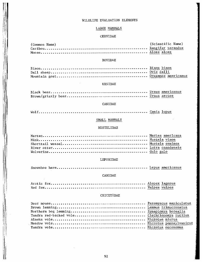
!I' !I' '
' :, I
(Common Name) Caribou. Moose •••
Bison •••.•• Dall sheep •• Mountain goat.
Black bear •••••••••• Brown/grizzly bear ••
WILDLIFE EVALUATION ELEMENTS
LARGE MAMMALS
CERVIDAE
BOVIDAE
URSIDAE
CANIDAE
(Scientific Name) Rangifer tarandus Alces alces
Bison bison Ovis dalli Oreamnos americanus
Ursus americanus Ursus arctos
Wolf. . . . . . . . . . . . . . . . . . . . . . . . . . . . . . . . . . . . . . . . . . . . . . . . . . . . . . . Canis lupus
Marten .• Mink •.•• Shorttail weasel. River otter •• Wolverine .•••
SMALL MAMMALS
MUSTELIDAE
LEPORIDAE
Martes americana Mustela vison Mustela erminea Lutra canadensis Gulo gulo
Snowshoe hare. . . . . . . . . . . . . . . . . . . . . . . . . . . . . . . . . . . . . . . . . . . . . . Lepus americanus
Arctic fox. Red fox ••••
Deer mouse ••••. Brown lemming ••• Northern bog lemming. Tundra red-backed vole •• Alaska vole •• Meadow vole •• Tundra vole ••
CANIDAE
CRICETIDAE
92
Alopex lagopus Vulpes vulpes
Peromyscus maniculatus Lemmus trimucronatus Synaptomys borealis Clethrionomys rutilus Microtus miurus Microtus pennsylvanicus Microtus oeconomus
BIRDS OF PREY
BUTEONINAE (Common Name) Bald eagle . .................... . Golden eagle •.....•.......•..... Red-tailed hawk •.•••••.•••••....•.••...• Harlan's hawk ••••••••• Rough-legged hawk •••••
American kestrel •••••• Gyrfalcon ••••••••••••• Merlin . ............ . Peregrine falcon ••••
FALCONINAE
ACCIPITRINAE
Goshawk .•••. .......•.. Sharp-shinned hawk ••••
Great horned owl ••• Great gray owl •••••• Hawk owl • ........... Short-eared owl •••••• Snowy owl ..........•.
STRIGIDAE
UPLAND BIRDS
TETRAONIDAE
Ruffed grouse •••• Spruce grouse. . . . . . . . . . . . . . e •••••••••••••
Rock ptarmigan. ~ ........................... . White-tailed ptarmigan •••••••••••••••• Willow ptarmigan •••••..••••••..••.••..•.
Robin . ......•....... Gray-checked thrush. Hermit thrush ••••••••• Varied thrush .••••••.••••...•• Vlhea tear • •••••••••••••••••••••
TURIDIDAE
93
(Scientific Name) Haliaeetus leucocephalus Aquila chrysaetos Buteo jamaicensis Buteo _h harlani Buteo lagopus
Falco sparverius Falco rusticolus Falco columbarius Falco peregrinus
Accipiter gentilis Accipiter striatus
Bubo virginianus Strix nebulosa Surnia ulula Asio flammeus Nyctea scandiaca
Bonasa umbellus Canachites canadensis Lagopus mutus Lagopus leucurus Lagopus lagopus
Turdus migratorius Catharus minimus Catharus guttatus Ixoreus naevius Oenanthe oenanthe
(Common Name) Pine grosbeak •••••••••••• Gray-crowned rosy finch •• Redpoll . ............... . White-winged crossbill. Savannah sparrow. Dark-eyed junco. Tree sparrow ••••• White-crowned sparrow. Lapland longspur. Snow bunting ••••.
Gray jay . ........... . Black-billed magpie •• Common raven •••••••••
Canada goose ••••.•••••••.•• White-fronted goose .•••••• Snow goose •••••••••••
American green-winged teal •• Mallard. Pintail. American wigeon •• Northern shoveler ••
Greater scaup •••••••• Lesser scaup ••••••. Barrow's goldeneye •• Oldsquaw •••••••• Harlequin duck •• King eider •••••• White-winged scoter ••
Trumpeter swan •••• Whistling swan ••••
FRINGILLIDAE
CORVIDAE
WATERFOWL
ANSERINAE
ANATINAE
AYTHYINAE
CYGNINAE
94
(Scientific Name) Pinicola enucleator Luecosticte t
--"-----...::..:::-=.::.~; Carduelis spp. Loxia leucoptera Passerculus Junco hyemalis Spizella arborea Zonotrichia leucophrys Clacarius lapponicus-Plectrophenax nivalis
Perisoreus canadensis Pica pica Corvus corax
Branta canadensis Anser albifrons Chen caerulescens
Anas crecca Anas platyrhynchos Anas acuta Anas americana Anas clypeata
Aythya marila Aythya affinis Bucephala islandica Clangula hyemalis Histrionicus histr Somateria spectabilis Melanitta deglandi
Olor buccinator Olor columbianus
OTHER WATER/MARSH BIRDS
GAVIIDAE (Common Name) (Scientific Name) Arc tic loon. • • • • . • • • • • • • • • • • . • • • • • • . • . • • • . • • • • • • • . • • • • • • Gavia arc tic a Connnon loon. . . . . . . . . . . . . . . . . . . . . . . . . . . . . . . . . . . . . . . . . . . . . Gavia imm.er
SCOLOPACIDAE
Common snipe ••..••••••••••••.•••••..•••.••••••.•..•.•.•• Capella gallinago Upland sandpiper. • • • • • • . • • • • • • . • . • • • • • • • • • • • • • • • • . • • • • . • Bartramia longicauda Spotted sandpiper •••••••••.•••..•••.••.••••••••••••..••• Actitis macularia Solitary sandpiper ••••••••••••.••.•.••.•••••••.••.•••••• Tringa solitaria Wandering tattler •.••.••••.••••.•••••••.•••••••••.•.•••. Heteroscelus incanus Lesser yellow legs. . • . • • • • • • . • • • . . • • • • • • • • • • • • • . • . • • • • • • • Tringa flavipes Baird's sandpiper. . • . • • • • • • • • • • . • • . • . • • . • • • • • • • • • • • . • • • • Calidris bairdii Dunlin. • • • . • • . • • • • . • • • • • • • . • • • • • • • • . • • • • • • • • • • . • . • • • • • • • Calidris alp ina Pectoral sandpiper. • • • • • . • . • . . . • • • . • • • • • • • • • • • . • . • • • • • • • Calidris melanotos Semipalmated sandpiper .••.•••••.•••.••••••••••.•.••••.•• Calidris pusilla
PHALAROPODIDAE
Northern phalarope ••••.•••••.••••...••..•.••.•.•.••••.•• Lobipes lobatus Red phalarope. • • . • . • • • • • • • • • . . • • • • • • • • • • • • • • • • . • • • • • • • • • Phalaropus fulicarius
CHARADRIIDAE
American golden plover ••••••.•••••..••••••...••••.••.•.• Pluvialis dominica Black-bellied plover .••••.•••.••••••.•••••••••..•.•••••• Pluvialis squatarola Semipalmated plover ••••••••••••.••••••••••••••..••••.... Charadrius semipalmatus
95
Appendix IV: Rating Entries and Contingency Tables
96
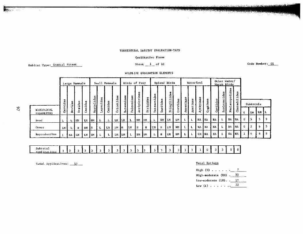
TERRESTRIAL IIABITA'r EVALUATION-TAPS
Qualitative fhuse
Sheet 1 of 12 Code Nrnnber:~-
WILDUFE EVALUATION ELEMENTS
l.arge Nammals Smull Mallllnuls Birds of Prey Upland Birds Waterfowl Other Water/ M' ·"h irds
Ill Ill
<II QJ QJ 'tl QJ
Ill <II
~ <!I .,; .,
(!) Ill (!) Ill s:l ~ 'tl 'tl 'tl ., Q) <!I :I ~ .,; Ill Q) ~
.,; 0 .... Q) 'tl ., 'tl ... Ill .,; QJ .-i QJ ] Ill OJ OJ 0 p.. .,; ., OJ Ill •(II ·rl 'tl (!) .,; .,; ·a .... 'tl l:l ., :;.1 Ill ~ ~ 3 Ill ., 0 ,.. "'
., ., Ill ,...j .,; ., .... d .... .,; 0 'tl 'tl "' p.. ... 'tl Sbbtotals .,.; 'tl 'tl :;l Ill H :;l Q) g 0 p.. btl Ill .,.; btl t ,.. .,; :>-. .... ·rf ;l 01 01
~ .... .,.; ... 0 tJ (J •rl ·rf ... 'tl s:l 41 ... ..::: c ·rf ,...j ... IHOI.Ol.:lf:AL ? Ul ~ II) p.. ~ .,; .... .-i 0 H .... '"' •rl Ill ., ... llO :> 0 ~ ~ 111 0 ... :il Q) H Jl "' (J ... 41 ::1 H 0 .'il .'il ~ ..... 01 0
PA l<A~!I('f" ItS (.."1 IQ p (.."1 ...:l (.."1 (.."1 11< ....; Ul £-< E-1 11< (.."1 (.."1 (,!) til 1'4 (.."1
H liM LM L
l'ooJ L L HM LH HH L L LM LM L HM HM L HH LM LM L L NA NA NA L NA NA 0 5 5 9
(:over LM L H HM H L JJ-1 LM H LM I! H U1 H LM HM L L NA NA NA L NA NA 6 2 6 5
Rl:lp rodut:t ion L NA LM LM HM L L U1 LM L liM HM L H LM HM L L LM NA NA L NA NA 1 4 6 8
Total Applications: _2_ __ _ Total Ratings
High (II) • • .
High-moderate (liM) 11
!.ow-moderate (LM). _...;:!1:.!.7 __
Low (L) •• , • • • • 22
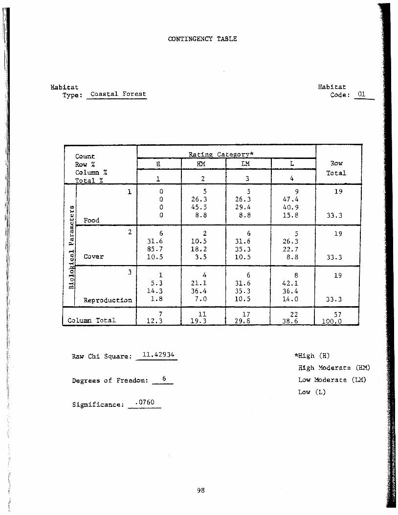
~~
il· I
' i q,
CONTINGENCY TABLE
Habitat Type: Coastal Forest
I Count Rating Category* Row% H HM L"f Column %
l Total % 1 2 3
1 0 5 5 0 26.3 26.3
(1.1 0 45.5 29.4 ).I Q.l 0 8.8 8.8 .1.1 Food Q.l e co 2 6 2 6 ).I
I co 31.6 10.5 31.6 ~
.-1 85.7 18.2 35.3 aS Cover 10.5 3.5 10.5 C;;l
.,..;
.g 3 1 4 6 .-1 0 5.3 21.1 31.6 .,..;
!XI 14.3 36.4 35.3 Reproduction 1.8 7.0 10.5
7 11 17 Column Total 12.3 19.3 29.8
Raw Chi Square: 11.42934
Degrees of Freedom: __ 6_
Significance: _._0_7_6_0 _
98
L
4
9 47.4 40.9 15.8
5 26.3 22.7 8.8
8 42.1 36.4 14.0
22 38.6
Habitat Code: 01
Row Total
19
33.3
19
33.3
19
33.3
57 100.0
*High (FI)
High Moderate (!h~)
Low Moderate (L~)
Low (L)
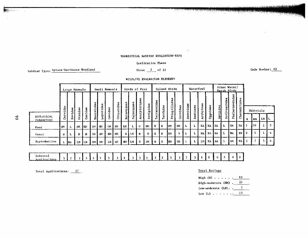
TERRESTRIAL IIABITA'f EVALUATION-TAPS
Qualitat:lve Phase
Habitat 'fylH>: Spruce-Deciduous Woodland Sheet 2 of 12 Code Number :_0_2 _
WIT.DLU'E EVALUATION ELEMENTS
Large Mmmuals Small Mammals Birds of Prey Upland Birds Waterfowl Other Water/ MRrRh irds
Q) Cll
Q) Q) Q) "" Q)
Cll Q) Cll "' .... Cll Q) Q) Q) Q) ;l ~ "" "" "" "" ~
Q) Cll Cll m Ql -rl Q) Q) •ri 0 -rl <U Cll "" 1:2 1-1 Cll -rl Q) rl Ql ] Ql "' Q) Ql u tl. -rl
"' ~ Q) ·Q) •rt "" Q) -rl •rt ·a ... "" 1:2 "' rl Cll Cll -~ -~ "' Cll 0 1-1
'tl ol "' rl •rt ol ... 1:2 ..-l ..-l 0 "" ..-l "" 1'1 "" p. 1-1 "" Subtotals ·.-1 "" "" :;! Q) 1-1 "" Q) 0 0 p. bO e •.-1 bO ..-l 1-1 •<"I 1:' :~ ~ Ill ., > ..-l ·ri ... 0 ..-l u Q) u ..-l ..-l "" l'l ~ Q) ... tl rl 1-1
Ill OLOG leAL ... > til ~ til p.
~ ·ri ... rl <J 1-1 ... 1-1 •ri (/) 01 ... bO > 0 ~ ~ Q) 0 l3 :il ~ k ;3 Cll :.! ... Q) ::1 t: 0 ~ ~ :>-. () Ill 0
PA I~ AM I~'!' I•: RS u o:tl u u o:tl 1<. til £-< £-< u < t:l til ~ u H liM LM L
Food HM L HM JIM JIM I!H HM HM LM L n JIM H H HM JIM L L NA NA NA L NA NA 3 10 1 5
Cover H L H H HH HM HM HM I! LM H II H H HM H L L NA NA NA L NA NA 9 5 1 4
Rcpruduet 1on L NA LM I,M HM liM LM liM HM LM H JIM H H liM HM L L LM NA NA L NA NA 3 7 5 4
'fotal Avpllcatlons: _...:5::...7~- Total Ratings
High (II) • • •
High-moderate (liM) 22
!.ow-moderate (LM). 7
Low (L) • • • • • • • __ 1_3_~
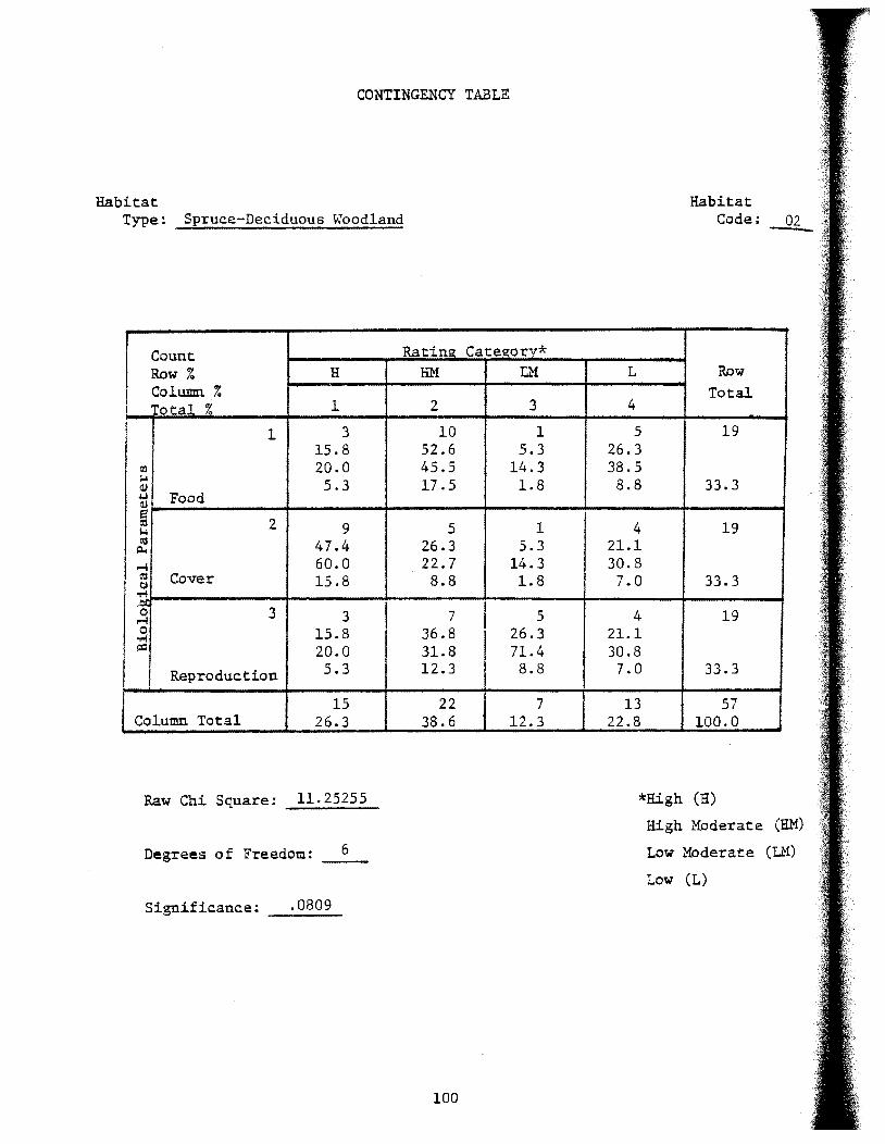
CONTINGENCY TABLE
Habitat Type: Spruce-Deciduous Woodland
Count Ratin12: Cate2orv* Row% H HM I.."!
Column % Total % 1 2 3
1 3 10 1 15.8 52.6 5.3
(Q 20.0 45.5 14.3 $.< 5.3 17.5 1.8 <U +.I Food <U
Ia 2 9 5 1 $.< cu 47.4 26.3 5.3 ~
I ...-! 60.0 22.7 14.3
I cu Cover 15.8 8.8 1.8 (;l
"'"" ·~ 3 3 7 5 """ 0 15.8 36.8 26.3 ...; ~ 20.0 31.8 71.4
Reproduction 5.3 12.3 8.8
15 22 7 Column Total 26.3 38.6 12.3
Raw Chi Square: 11.25255
Degrees of Freedom: __ 6_
Significance: .0809
100
L
4
5 26.3 38.5 8.8
4 21.1 30.8 7.0
4 21.1 30.8 7.0
13 22.8
Habitat Code:
Row Total
19
33.3
19
33.3
19
33.3
57 100.0
*High (H)
High Moderate (HM)
Low Moderate (~'1)
Low (L)
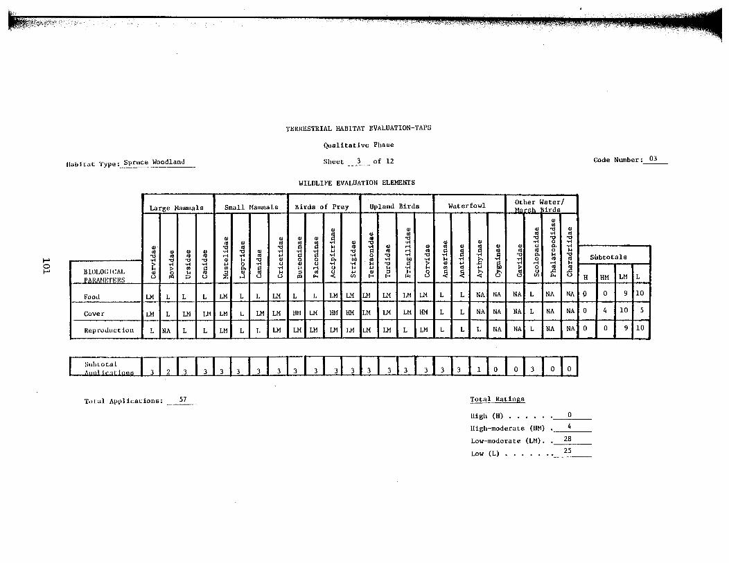
1-' 0 1-'
llal>i tat Type : __ ~pruce Woodland
Large Hannuals
Cl)•
"' Cl.l Cl.l 41 ., "' "' "' ·.-l ., ., .,
~ ·.-l ·.-l ·.-l
Bllll.OG ICAL :> Ul ~ Cl.l 0 ... PARANETERS 0 1"1 ::> 0
Food LM L L L
Cover LM L LM LM
Reproduce ion L NA L L
Total Applications: 57
Small Hammals
Cl.l Cl.l
~ Cl.l "' "' .,
·.-l ., Cl.l ·.-l .-1 ..-1 "' .... Q) ... ., Q) .... 0 ·.-l <J Ul p. ~ ·.-l
~ Q) H t-1 0 0
LM L L LM
LM L LM Ul
LM L L LM
TERRESTRIAL HABITAT EVALUATION-TAl'S
Qualitative Phase
Sheet 3 of 12
WILDLIFE EVALUATION ELEMENTS
Blrds of Prey Upland Birds
Cl.l Cl.l ., Cl.l ., Cl.l Cl.l 1:1 ., ., "' ~ •.-l Cl.l ., ·.-l 1:1 ... "' •.-l Cl.l .-1 Cl.l
·.-l ·a .... ., 1:1 "' .-1 "' 1:1 ·.-l ·.-l 0 ., •.-l ., 0 0 p. bl) "' ·.-l bl) •.-l Cl.l u ·.-l •.-l ... ., s:: ~ .... .-1 <J ... .... ... ·.-l ::J "' <J .... Cl.l ::l ... 0
1"1 I>< < Cll E-< E-< I>< 0
L L LM LM LM LM LM LM
11M LM 11M HM LM LM LM 11M
LM LM LM LM LM LM L LM
Code Number: OJ
Waterfowl Other Water/ Harsh irds
Cl.l ., Cl.l ., Cl.l ., ..-1 ., ., ., .,
~ Cl.l ·.-l 0 ·.-l Cl.l "' Cl.l Cl.l <J p. ·.-l
1:1 ~ 1:1 "' "' "' 0 ... ·.-l ·.-l .~
., p. ... ., Subtotals ... ·.-l .Ei' ..-1 0 "' "' Cl.l .... 1:1 ..-1 .-1 .-1 ...
Ul "' .... QD :> 0 "' "' ~ ~ :>-. ~ "' <J .c .c < l!l Cll p., 0 II HM LM L
L L NA NA NA L NA NA 0 0 9 10
L L NA NA NA L NA NA 0 4 10 5
L L L NA NA L NA NA 0 0 9 10
Total Ratings
High (II) • • • 0
High-moderate (HM) 4
Low-moderate (LM). 28
Low (L) • • • • • • •. __ zs __
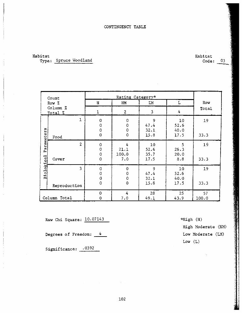
Habitat Type: Spruce Woodland
l Count Row% H Column % Total % 1
1 0 0
(1.1 0 l-4 aJ 0 -1-1 Food aJ = (ij 2 0 l-4 ca 0 p..
..-1 0
l ca Cover 0 Cl .....
I -~ 3 0 0 ..-1
I 0 0 ..... ~ 0
I Reproduction 0
I 0 j Column Total 0
Raw Chi Square: 10.07143
Degrees of Freedom: 4
Significance! .0392
CONTINGENCY TABLE
Rating Category* HM L.'1
2 3
0 9 0 47.4 0 32.1 0 15.8
4 10 21.1 52.6
100.0 35.7 7.0 17.5
0 9 0 47.4 0 32.1 0 15.8
4 28 7.0 49.1
102
L
4
10 52.6 40.0 17.5
5 26.3 20.0 8.8
10 52.6 40.0 17.5
25 43.9
Habitat Code: 03
Row Total
19
33.3
19
33.3
19
33.3
57 100.0
*High (H)
High Moderate (HM)
Low Moderate (k'1)
Low (L)
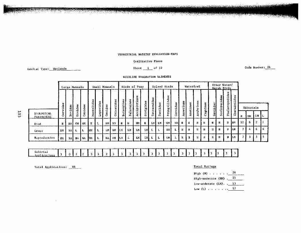
..... 0 w
Uald Lat '1'ypc
J.arge Mun~nals
<1.1 01 Q) Q) <II 'tl "' "' "' •ri 'tl 'tl ~ > •ri .,.;
BIOLOGICAL H > UJ ~ 0) ~ ~ PARMU<:TERS u u
Food H NA HM liM
Cover HM NA L L
Reproduction HM NA NA NA
Total Application;;: 66
Small Mannnals
0) Q)
"' 0) 01 'tl "' 'tl ·ri 'tl 0) .,; ..-! •ri "' ... Q) ... 'tl Q) ... 0 .,.; u Ul g. l:l •ri
:i! Ill .... ...:1 u u
H L HM HH
HM L LM llt!
HM L NA HM
'rERIU:S'l'RIAL HABITAT EVALUATION-TAPS
Qualitative Phase
Sheet of 12
WILDLIFE EVALUATION ELEMENTS
Birds of Prey Upland Birds
Cl) Cl)
01 Cl) 01 Q) 0) l:l .:g 'tl
"' m •ri Q) ·ri l:l .... 01 .,.; Cl) ..-! Q)
•ri •ri ... 'tl l:l "' ..-! 01 l:l l:l .,; .,; 0 'tl .,.; 'tl 0 0 "' tJQ '<II .,; t>IJ •ri 0) <.1 ..-1 .,; .... 'tl l:l e ... ..-! u .... ... H ·ri :;! 01 ~ ... Cl) :;! .... 0 ~ ~ "' 1:-< 1:-< ~ u
H H liM H LM LM HM liM
I.M LM LM U! L L liM L
LM L I..M Ul L L LM L
Q)
] H Q)
~ H
H
H
Code Number: 04
Waterfowl Other Water/ Marsh irds
Q)
01 Q) 'tl Q)
01 •ri "' 'tl 'tl 'tl 0) ·ri 0 ·ri
Q) 01 Q) Q) u "' .,.;
"' "' 0 .... m .~ ] 'tl "' .... 'tl Subtotals •ri :>-. :~ 0 Ill <11 ... 01
.'a
H
H
H
.<:1 g, ..-! ..-! .... ... > 0 ~ ~ :>-. :>-. 01 0 < u (!) "' P-; u H
H H H H H HM 12
u H H H H LM 7
H H H H H LM 7
Total Ratings
High (H) • • • 26
High-moderate (llt!) __ 1_5 __
Low-moderate (LM). --=lc-=:3 __
Low (L) • • • • • • ·--~1=2 __
liM LM L
8 2 1
4 6 6
3 5 5
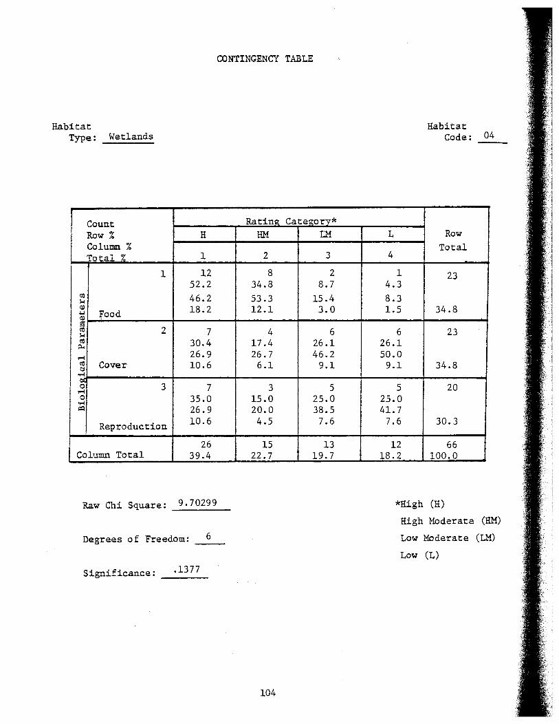
Habitat Type: Wetlands
Count Row% H Column % Total % 1
1 12 52.2
C1l 46.2 l-1 (1) 18.2 .j.J Food (1) e tO 2 7 l-1 tO 30.4 j:l..j
l .-l 26.9 tO Cover 10.6 ~ ~
~ 3 7 .-l 0 35.0 ..... ~ 26.9
Reproduction 10.6
26 Column Total 39.4
Raw Chi Square: 9.70299
Degrees of Freedom: 6
Significance: .1377
CONTINGENCY TABLE
Rating Category* HM L.'1
2 3
8 2 34.8 8.7 53.3 15.4 12.1 3.0
4 6 17.4 26.1 26.7 46.2 6.1 9.1
3 5 15.0 25.0 20.0 38.5 4.5 7.6
15 13 22.7 19.7
104
L
4
1 4.3 8.3 1.5
6 26.1 50.0
9.1
5 25.0 41.7
7.6
12 18.2
Habitat Code: 04
Row Total
23
34.8
23
34.8
20
30.3
66 100.0
*High (H)
High Moderate (HM)
Low Moderate (L'1)
Low (L)
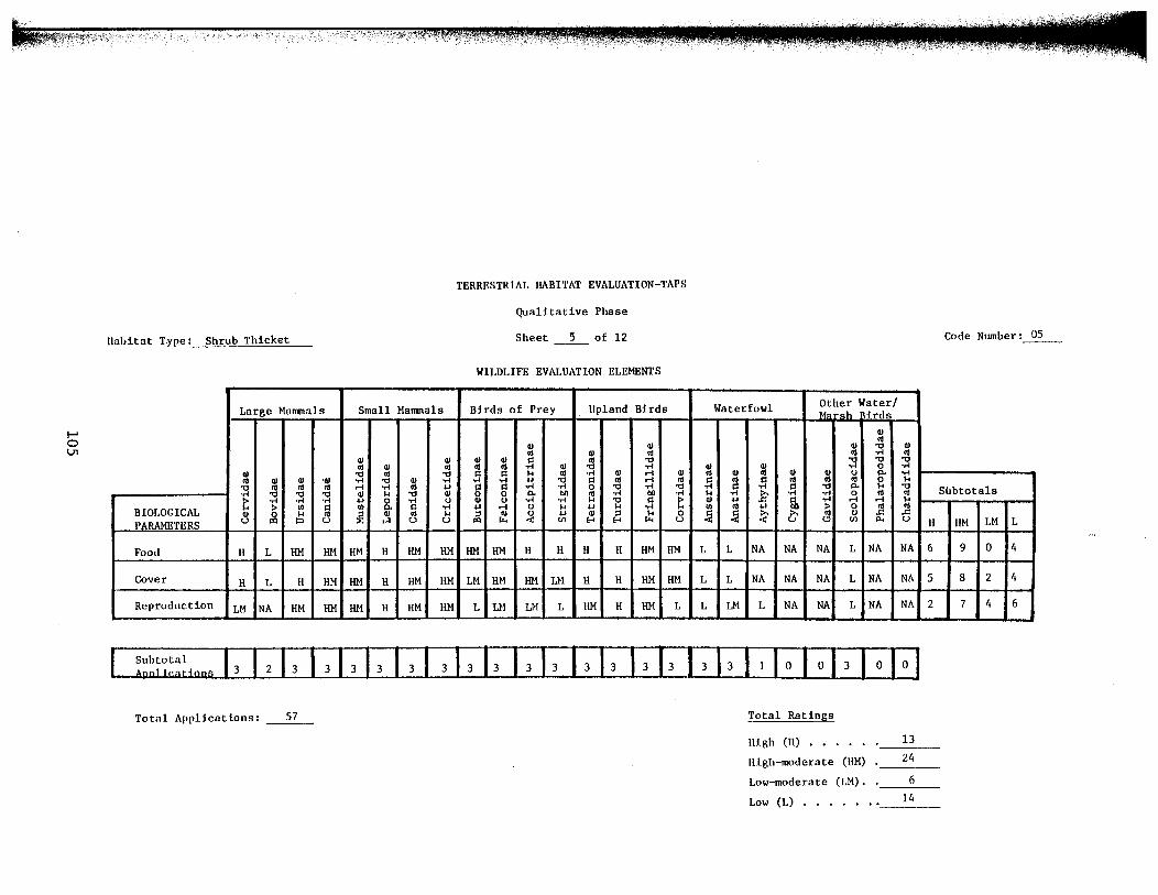
...... 0 I.J1
Habitat T:ype: Shrub Thicket
Large Mannnals
Q)
"' Q) Q) ·GJ '"0 "' "' "' ·.-1 '"0 '"0 '"0
~ oM •.-1 ·.-1
BIOLOGICAL :> Ill 1:1 Ql 0 ... "' PARAMETERS u IQ ::> u
Food H L HM HM
Cover H L H HM
Reproduction LM NA HM HM
Total Applicati.ons: _......::.5'-7-
Small Mannnals
Q) Q)
"' Q) "' '"0 "' '"0 •.-1 '"0 Ql •.-1 .-l ·.-1 "' ... Ql ... '"0 Ql ... 0 •.-1 u Ill p. ~ •.-1
~ Q) ...
...:1 u u
HM H HM HM
HM H HM HM
HM H HM HM
TERRESTRIAL HABITAT EVALUATION-TAPS
Qualitative Phase
Sheet 5 of 12
WILDLIFE EVALUATION ELEMENTS
Birds of Prey Upland Birds
Q) Q)
"' Q) "' Q) Q) ;; "' '"0
~ ~ Q) '"0 oM ... "' •.-1 Q) .-l Q)
•.-1 -a ... '"0 1:1 "' .-l "' 1:1 •.-1 ·.-I 0 '"0 oM '"0 0 0 p. bO "' ·.-1 bO ·.-1 Ql u ·.-1 ·.-1 ... '"0 1:1 ~ ... .-l u ... ... ... oM
~ "' ~ ... Ql ::l t:: 0
"'"' Ul H H u
HM HM H H H H HM HM
LM HM HM LH H H HM HM
L Ul Ul L HM H HM L
Q)
"' 1:1 oM ... Ql Ill
.'il
L
L
L
Waterfowl Other Water/
Q)
~ ·.-1 ... "' .'il
L
L
LM
M!'lr"h
Q)
"' '"0 Q) •.-1
"' Q) Q) u 1:1 ~ "' "' •.-1 '"0 p.
.t' ·.-1 ·.-I 0
~ oM .-l ... :> 0
~ (J 01 u (.!) Ul
NA NA NA L
NA NA NA L
L NA NA L
Total Ratings
High (11) • • •
111gh-modera te (HM)
Low-moderate (LM).
Low (L) . • . . .
irds Q)
"' '"0 ·.-1 '"0 0 p. 0 ... "' .-l
"' .c p.,
NA
NA
NA
Code Nwnber: OS
Q)
"' '"0 •.-1 ·.-1 ... '"0 Subtotals "' ... l! u H JIM LM L
NA 6 9 0 4
NA 5 8 2 4
NA 2 7 4 6
13
24
6
14
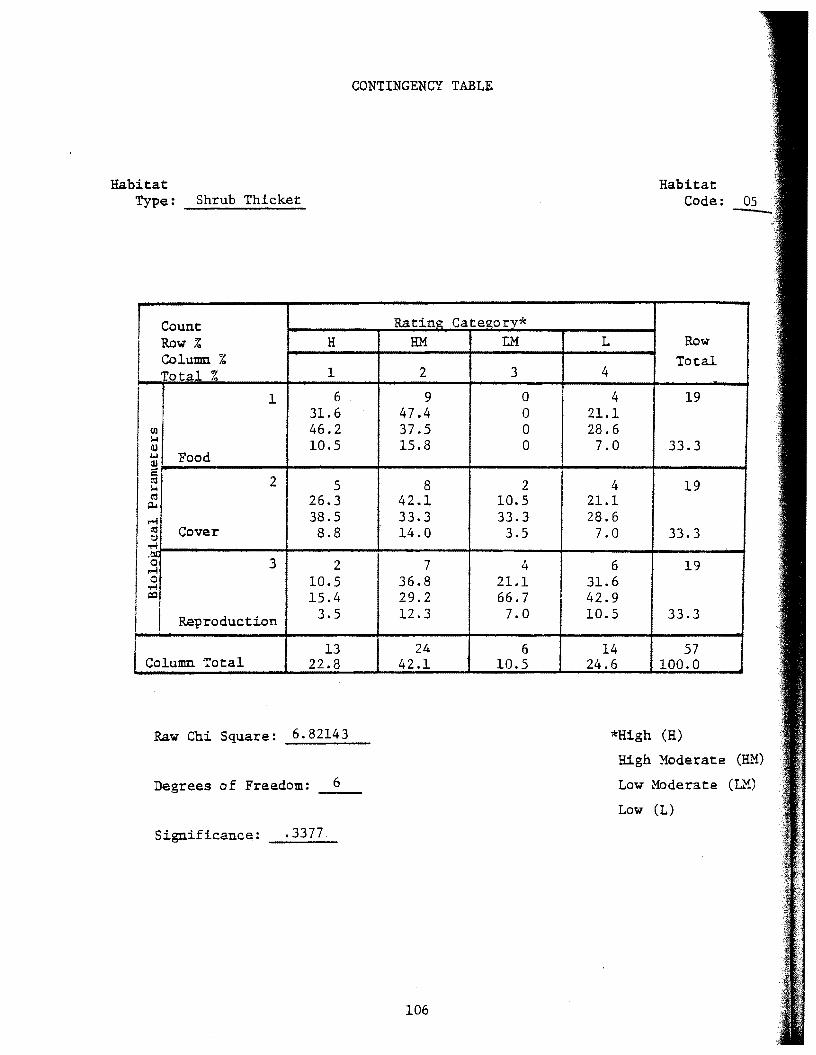
Habitat Type: Shrub Thicket
I Count Row% H Column %
! Total % 1
1 6 31.6
Ql 46.2 i-1 10.5
I (]) .w Food (])
~ i-1 2 5 <tl 26.3 ~
...... 38.5 as Cover 8.8 (;)
I ...-!
'o 3 2 ...... 0 10.5 .,..; ~ 15.4
Reproduction 3.5 I
13 Column Total 22.8
Raw Ch.i Square: 6. 82143
Degrees of Freedom: 6
Significance: .3377
CONTINGENCY TABLE
RatinSl: CateSl;orv* HM L.'i
2 3
9 0 47.4 0 37.5 0 15.8 0
8 2 42.1 10.5 33.3 33.3 14.0 3.5
7 4 36.8 21.1 29.2 66.7 12.3 7.0
24 6 42.1 10.5
106
L
4
4 21.1 28.6 7.0
4 21.1 28.6 7.0
6 31.6 42.9 10.5
14 24.6
Habitat Code:
Row Total
19
33.3
19
33.3
19
33.3
57 100.0
*High (H)
High Moderate
Low Moderate (L'i)
Low (L)
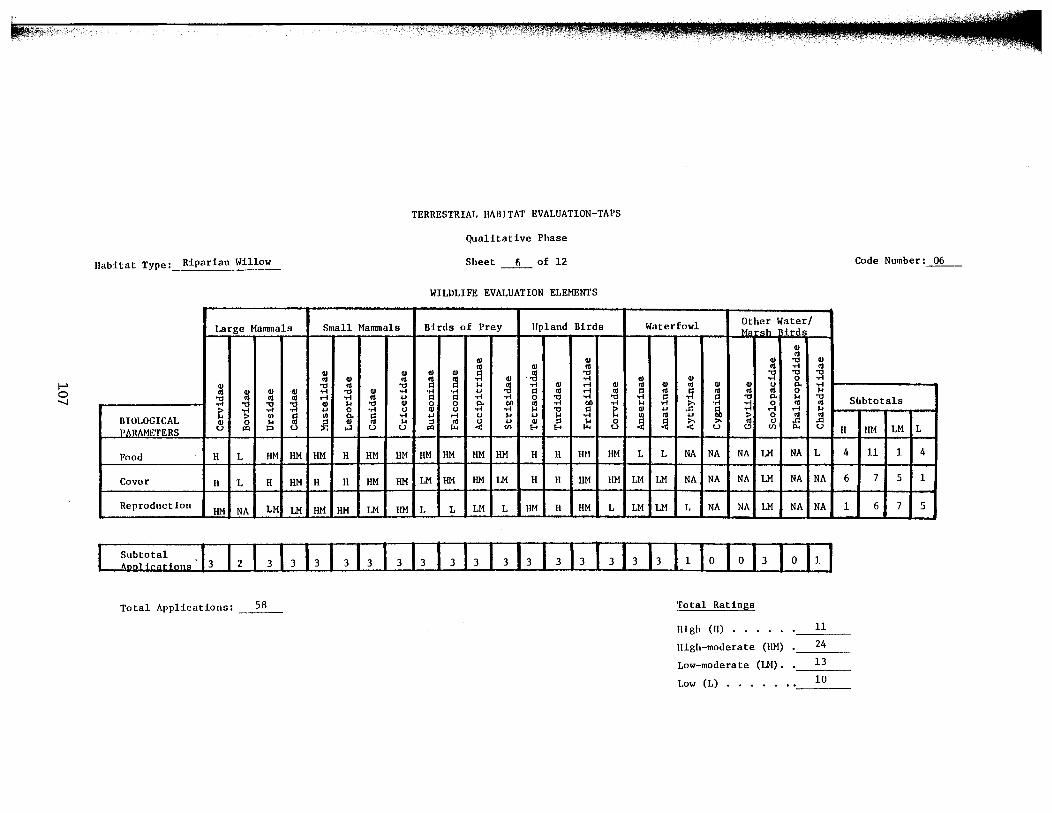
TERRESTRIAL I~BITAT EVALUATION-TAPS
Qualitative Phase
Habitat Type: Riparian Willow Sheet _6_ of 12 Code Number:~
WILDLIFE EVALUATION ELEMENTS
Large Mammals Small Mammals Birds of Prey Upland Birds Waterfowl Other Water/ Marsh irds
Q)
"' Q) Q) Q)
""' Q)
"' Q) "' "' ..-1 "' Q) Q) Q) Q) ~ "' ""' ""' ""' ""' "' Q) "' "' m Q) ·"tl ..... Q) Q) ..... 0 . .... Q)
""' "' ""' s:l ... "' ..-1 Q) .-i Q) "' Q) "' Q) Q) (.) p. ..-1
"' Q) Q) ·CIJ ..... ""'
Q) ..-1 . .... ..... +' ""' s:l "' :;:l "' s:l "' .~ "' "' "' 0 ... ""' "' "' "' .-i ..-1 "' ... s:l s:l ..-1 . .... 0 ""' ""' ..-1 s:l s:l ""'
p. ... ""' Subtotals ..... ""' ""' ""'
Q) ... ""' Q) 0 0 p. t>O "' ..-1 t>O ..-1 ... ..... .t' . .... :~ 0 "' "' ~
..... . .... ·.-1 ... 0 ·.-I (.) Q) rJ ..-1 ..-1 ... ""' s:l ~ Q) ... {;, .-i .-i ... BIOLOGICAL > Ill g Ill go g ..-1 ... .-i (.) ... +' ... .....
] "' ... ~ 0 "' "' Q) 0 ... jl ... ::! "' ~ +' Q) ::! ... 0 !il ~ :>- (.) ..:: ..:: PARAMETERS tJ IXl ::::> tJ H tJ tJ IXl ~ U) H H ~ tJ tJ (.!) U) p., tJ II liM LM L
Food H L HM HM HM H HM 11M HM HM HM HM H H HH liM L L NA NA NA LM NA L 4 11 1 4
Cover II L H liM H H HM 11M LM 11M 11M LM H H 11M liM LM LM NA NA NA LM NA NA 6 7 5 1
Reproduction 11M NA LM LM liM HM LM HM L L LM L 11M H HM L LM LM L NA NA LM NA NA 1 6 7 5
Total Applications: 58 Total Ratings
High (II) • • • 11
High-moderate (HM) 24
Low-moderate (UI). 13
Low (L) . • . • . . • 10
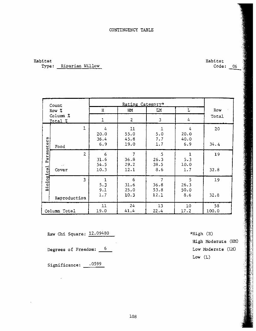
CONTINGENCY TABLE
Habitat Type: Riparian Willow
I Count Rating Cateszorv* Row % H HM L'1 Column % Total % 1 2 3
1 4 11 1 20.0 55.0 5.0
Ol 36.4 45.8 7.7 ,... QJ 6.9 19.0 1.7 .... Food QJ s ~ 2 6 7 5 ,... ~ 31.6 36.8 26.3 ~
,...; _) 54.5 29.2 38.5 ~ Cover 10.3 12.1 8.6 C.l ~
0 3 1 6 7 ,...; 0 5.3 31.6 36.8
...-! ~ 9.1 25.0 53.8
I Reproduction 1.7 10.3 12.1
j Column Total 11 24 13
19.0 41.4 22.4
Raw Chi Square: 12.09480
Degrees of Freedom: __ 6_
Significance: .0599
108
L
4
4 20.0 40.0 6.9
1 5.3
10.0 1.7
5 26.3 50.0 8.6
10 17.2
Habitat Code: 06
Row Total
20
34.4
19
32.8
19
32.8
58 100.0
*High (H)
High Moderate
Low Moderate (L~)
Low (L)
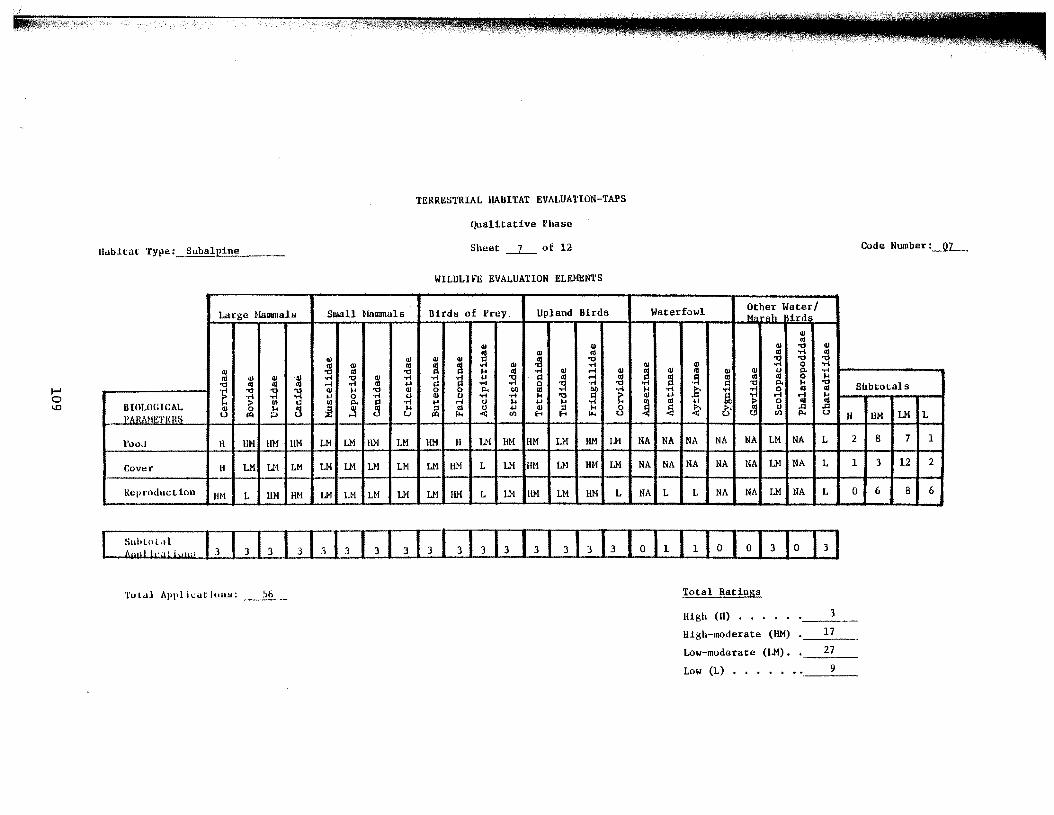
TERRESTRIAL HABITAT EVALUATION-TAPS
Qualitative Phase
Uabitat Type: Subal,.~:P:.=i!!n::::e ___ _ Sheet~ of 12 Code Nwnber :_91__
WILDLIFE EVALUATION ELEMENTS
Large Mammals Small Mammals Birds of Prey Upland Birds Waterfowl Other Water/ Ma ·sh irds
<I)
<I) <I) "' <I) 'tl <11 111 <11 111 "' oM "' <I) 4) <11 <11 .!'l "' 'tl 'tl 'tl ~ ., 4) ~ ~ ~ w ~ ·rl
~ 4) oM 0
w ~ "' .... <II Ill .-1 <11 Ill 111 <I> w <J "" oM <II ~
Q) ·Ill ~ ~ oM ·rl -a ... 'tl l:l "' .-1 111
~ -~ 111 Ill Ill 0 .... 'tl <II Ill .-1 +' l'l ""' ·rl
~ 'tl •rl 'tl •rl .!'l 'tl p.
~ 'tl •.-I 'tl 'tl 'tl \11 .... 'tl Ill ~ 0 p. Ill) ·rl Ill) •rl .... ~ ~ ~ "' Subtotals t ·rl .,.; ..... ... 0 .,.; (J ;j •rl •rl 'tl 1:1 ~ Q) ... a .-1 ....
BIOLOGICAL ~ Ill 3 Ill p. 3 ·rl ... <J .... ... .... .,.;
~ Ill ... > 0 ~ tl <I) .... :f <I> .... :;1 ~ ;;] ... <I) ::1 .... 8 ~ ~ Is' 111 (J
P6BAH!"l'ERS u ltl p t-1 u ltl 00
"'"' "'"' .... (.!) Cll p.. II LM L liM
Foot.! H liM liM liM LM LM liM I.M HM H LM HM HM LM HM LM NA NA NA NA NA LM NA L 2 8 7 1
Covtor H LM LM LM LM LM LM LM LM liM L LM HM LM liM LM NA NA NA NA NA LM NA L 1 3 12 2
Reproduction liM L liM HH LN LM LM LM LM liM L LM liM LM HH L NA L L NA NA LM NA L 0 6 8 6
'l'ut.tl Appl h:atJoa:;: ___ .. ::..:::.. ·- Total Ratings
High (H) • • • 3
lligh-moderate (HM) 17
Low-moderate (LM). 27
Low (L) • • • • • • • 9
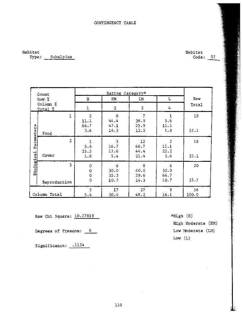
Habitat Type: Subalpine
Count Row,% Column % Total %
1
rn ,... QJ ~ Food QJ s ell 2 ,... ell
p..
.-1 ell Cover tJ
...... ·~ 0 3 ,..., 0
'l"'i ~
Reproduction
Column Total
H
1
2 11.1 66.7
3.6
1 5.6
33.3 1.8
0 0 0 0
3 5.4
Raw Chi Square: 10.27819
CONTINGENCY TABLE
Ratin12: Cate12:orv* HM LM
2 3
8 7 44.4 38.9 47.1 25.9 14.3 12.5
3 12 16.7 66.7 17.6 44.4 5.4 21.4
6 8 30.0 40.0 35.3 29.6 10.7 14.3
17 27 30.4 48.2
Degrees of Freedom: __ 6_
Significance: .1134
110
L
4
1 5.6
11.1 1.8
2 11.1 22.2 3.6
6 30.0 66.7 10.7
9 16.1
Habitat Code: 07
Row Total
18
32.1
18
32.1
20
35.7
56 100.0
*High (H)
High Moderate (RM)
Low Moderate (L4~)
Low (L)
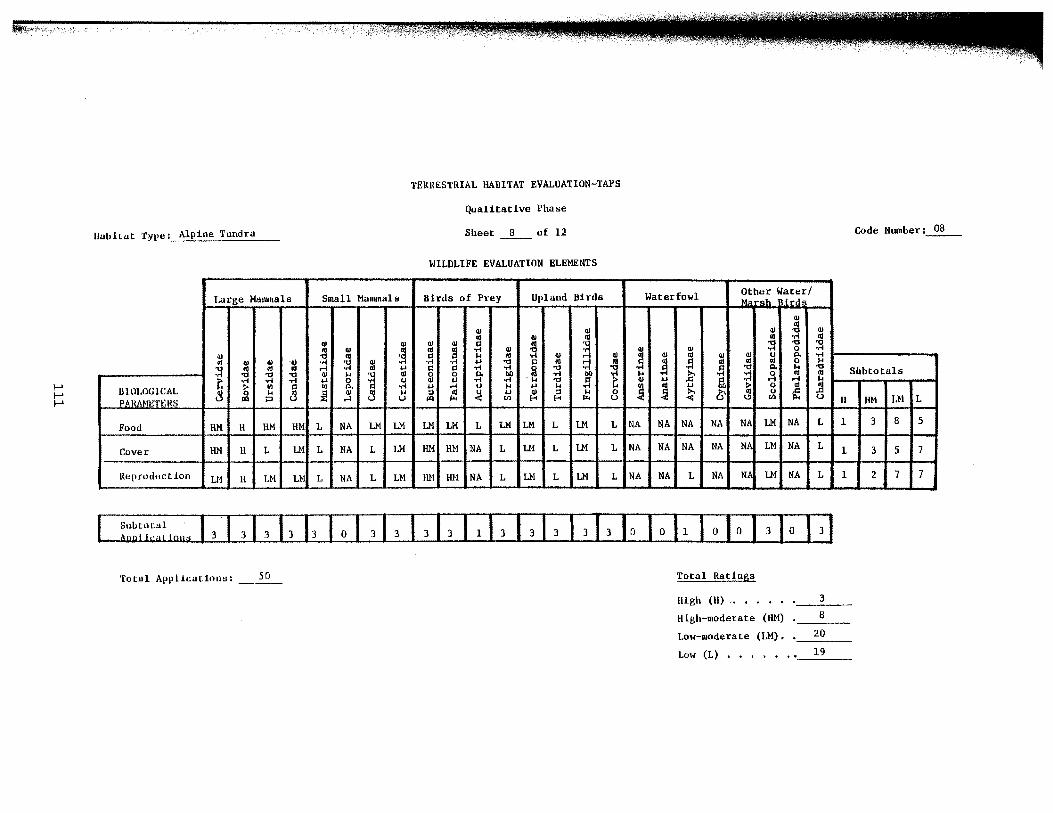
'l'ERRESTlUAL HABITAT EVALUATION-TAPS
Qualitative Phase
Uabil.at 'f,ype: Alpine Tundra Sheet of 12 Code Number:~
WILDLIFE EVALUNfiON ELEMENTS
I.arge Mammals Small Mal!llnals Birds of Prey Upland Birds Waterfowl Other Water/ Marsh ird
Q) qj
Q) Q) Q) ..., Q)
<G Q) <G Ill .... <G Q)
~ Ql Ql ~ ~ "'CI ;I "'CI "'CI
~ Ql ~ .§ \1) .,.;
31 Ql 0 .,.; Ql <G ;I ... 01 Q) rl \1) Qj
~ ~ Q) 0 p.. .,.;
<G Q) fl) ·Ill .... ;I lll .,.; .... "'CI ~ .,
:;:1 "' ~ -~ Ill ., 0 ...
;I <G 01 "' rl .... ~ l'l .,.; .,.; 0 "'CI "'CI ~ "'CI p.. ... "'CI Subtotals "'CI "'CI ;I Ql ... ~
Q) 0 0 !7 !>() "' .,.; ! .,.; ... ~ :::l 0 "' <11
r. .... .,.; .... 0 0 \1) u .,.; . ... "'CI t Ql .... a rl ';;t ~ IHOI.OGlCAL ~ Ul 5 Ul p.. .,.; .... rl <.1 ... .... !;! ~ ! .... ~
0 QJ ... :il Ql 01 ... ~ <11 ~ .... Ql ... 0 :>. & 0 .d
PARAH~'n:RS u IQ p ,.:! u u '"' 1/) E-< E-< '"' u < <1.1 p.. u II HM LM L
Food HM H HM liM L NA LM LM LM LM L LM LM L LM L NA NA NA NA NA LM NA L 1 3 8 s
Cover 11M ll L LM L NA L LM 11M HH NA L U1 L LM L NA NA NA NA N/ LM NA L 1 3 5 7
Reproduction Ll1 H LM LM L NA L LM liN ill! NA L LH L LM L NA NA L NA Nl LM NA L 1 2 7 7
Total Appllcutilllll>: 50 Total Ratings
High (ll) • , ,
High-moderate (HM) 8
!.ow-moderate (LM), 20
Low (L) , •••• , • 19
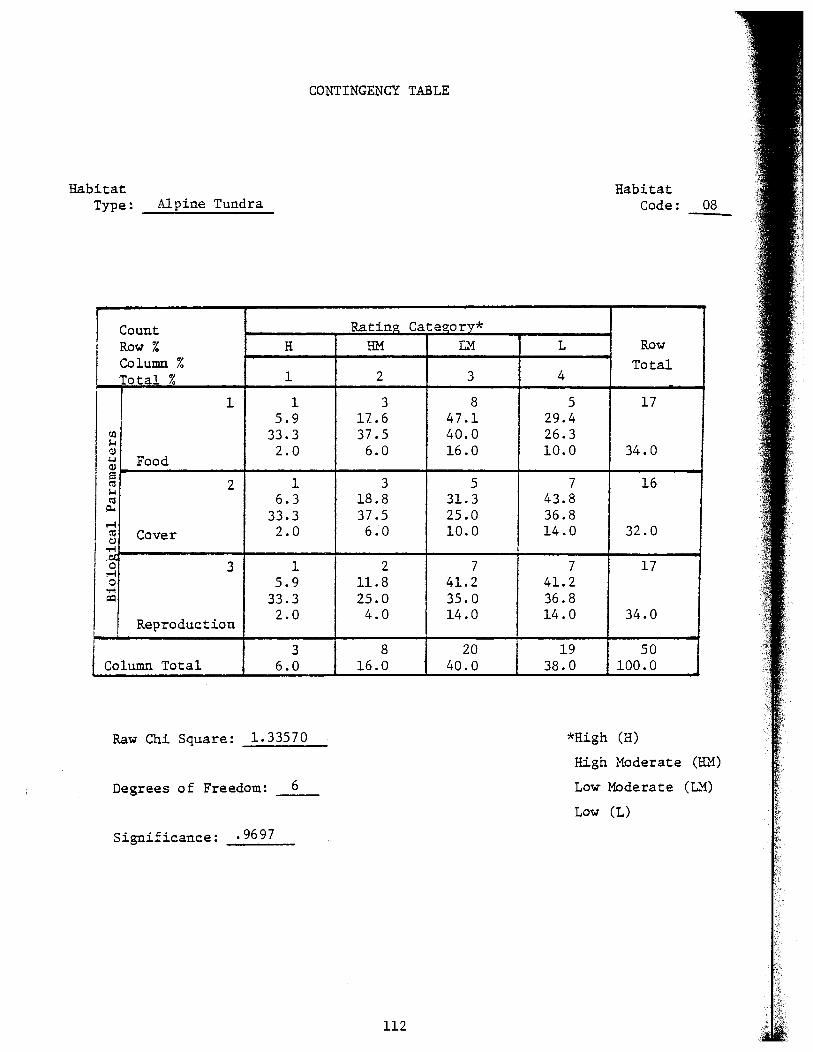
Habitat Type: Alpine Tundra
I Count Row % H Column % Total % 1
1 1 5.9
en 33.3 ~ a) 2.0 .u Food a)
6 1 ell 2 ~
6.3 ell p..
33.3 I '""' 2.0 I ('d Cover
Cl "1'-l ·~ 3 1 0
'""' 0 "1'-l
5.9 I:Q 33.3
t Reproduction 2.0
I Column Total 3
6.0
Raw Chi Square: 1.33570
Degrees of Freedom: 6
Significance: .9697
CONTINGENCY TABLE
Rating Category* HM L.'1
2 3
3 8 11.6 47.1 37.5 40.0
6.0 16.0
3 5 18.8 31.3 37.5 25.0 6.0 10.0
2 7 11.8 41.2 25.0 35.0 4.0 14.0
8 20 16.0 40.0
112
L
4
5 29.4 26.3 10.0
7 43.8 36.8 14.0
7 41.2 36.8 14.0
19 38.0
Habitat Code: 08
Row Total
17
34.0
16
32.0
17
34.0
50 100.0
*High (H)
High Moderate (1h'1)
Low Moderate (L'1)
Low (L)
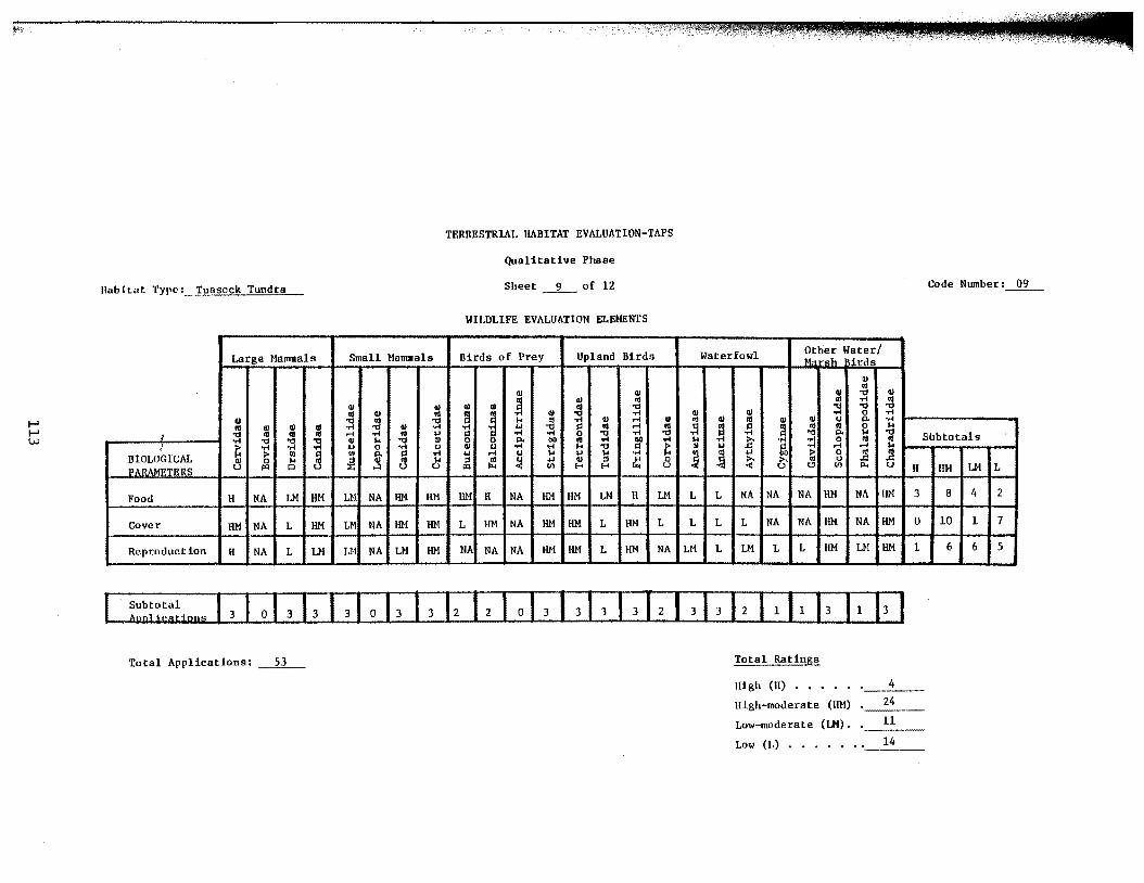
llab ltut 'l'ypt' :_ . .'!:1!1!1Sock Tundra
Large Mammals
' ; BIOLOGICAL PARAMETERS
Food
Cover
Reproduction
Subtotal Appl !rations
Q) ., '1:1 •.-1
~ Q) u
H
HM
H
Q) Q) ., Ill '1:1 :;1 .... ~ (I) ...
1<1 p
NA LM
NA L
NA L
Total Applicat:l.ons: _ _,5:.::3:___
= :;1
~
HM
HM
LM
Small Mammals
Q) II) Ill II) Ill 'd ., '1:1 .... '1:1 II) .... .... .... Cll ... II) ... '1:1 Q)
u 0 s <.> (I) p. .... :i! II) ...
...:1 u
LM NA HM HM
LM NA HM HM
LM NA LM HM
TERRESTRIAl. IIABITAT EVALUATION-TAPS
Qualitative Phase
Sheet _9_ of 12
WILDLIFE EVALUATION ELEMEN'l'S
Birds of Prey Upland Birds
Ql Q)
Q) ] II) Cll II) ~ '1:1
! ~ Q) .... ... ., .... Ql .... m ... '1:1 s:: Ill :;:j 1:1 ..-! ..-! 0 '1:1 '1:1
~ 0 p. !lO ., .... !lO ..-! u .... .... ... '1:1 d ~ ... .... u "' ... ... ·.-1
::1 &! .'A ... Cll ::1 ~ 0 1<1 Ul !-< !-< u
HM H NA HM HM 1M H LM
1 HM NA HM HM 1 HM L
NA NA NA 11M HM L 11M NA
Code Number :___Q2__
Waterfowl Other Water/ M' rsh lirds
Ql Cll
Q) '1:1 Q)
Ill .... ~ :;1 'd
:s Q) 0 Q) ., II) II) u p. ....
~ ! ~ Ill Ill Ill 0 "' J:: '1:1 p. "' '1:1 Subtotals "' %:' .... ..-! 0 Ill ., II) ... tt .... .-1 .-1 ] ~
<II ... ~
0 ~ .lii !{ :>, u u Ul I>< u H liM LM L
L L NA NA NA HM NA liM 3 8 4 2
L L 1 NA NA 1:!}1 NA HM 0 10 1 7
LM L LM L L 11M LH HM 1 6 6 5
Total Ratings
High (H) • • •
High-moderate (liM) 24
Low-moderate (LM). 11
Low (L} • • • • • . • 14
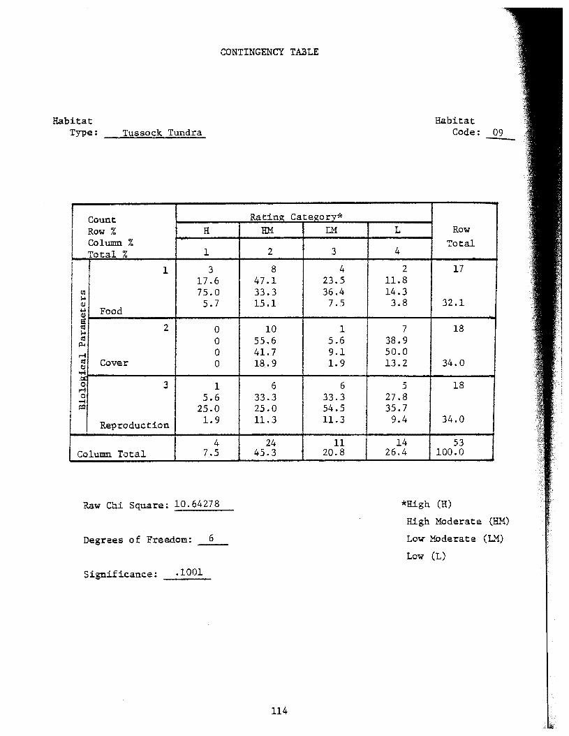
Habitat Type: Tussock Tundra
[ Count Row % H Column % Total % 1
1 3 17.6
rn 75.0 ,_ (]) 5.7 .u Food (])
I e \'0 2 0 ,_ \'0 0 p..
...... 0 \'0 Cover 0 tl
.,..; ·~
3 0 1 ...... 0 5.6 .,..;
::Q 25.0
Reproduction 1.9
4 Column Total 7.5
Raw Chi Square: 10.64278
Degrees of Freedom: 6
Significance: .1001
CONTINGENCY TABLE
Rating Categorv* HM L.'1
2 3
8 4 47.1 23.5 33.3 36.4 15.1 7.5
10 1 55.6 5.6 41.7 9.1 18.9 1.9
6 6 33.3 33.3 25.0 54 .s 11.3 11.3
24 11 45.3 20.8
114
L
4
2 11.8 14.3
3.8
7 38.9 50.0 13.2
5 27.8 35.7
9.4
14 26.4
Habitat Code:
Row Total
17
32.1
18
34.0
18
34.0
53 100.0
*High (H)
High Moderate
Low Moderate (~'1)
Low (L)
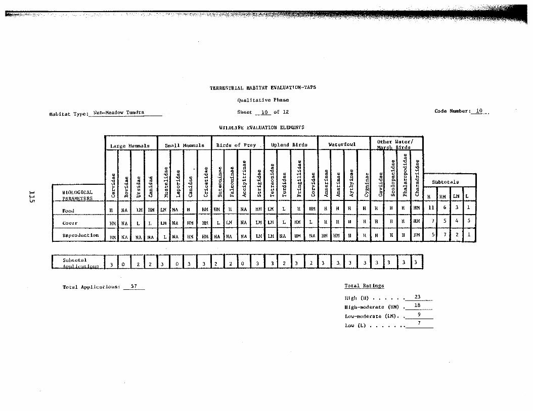
'l'ERRESTRIAL HABITAT EVALUA'riON-TAPS
Qualitative Phase
Habitat T:ype: Her-Meadow Tundra Sheet _lQ_ of 11! Code Nl.Ullber :_!Q__
WILDLIFE EVAI.UATION ELEMENTS
Large Hannnals Small Hammals Birds of Prey Upland Birds Waterfowl Other Water/ M~ ·sh irds
Gl
<II <II <II ~ Gl
m Gl ol ol .... ol <II . <II Ill Ill "' "CC "CC "CC ~ Ill <II ol ~ ~
·.-t Gl "CC .... at Ill .... 0 Gl "CC ol "' ... ~ .... Ill .... Gl Ill Ill Ill Ql 0 ll. .... ol Ql ~ '$ ·.-t "CC ::1 .... ·.-t ... p ol .... ~ .;j .~ .~
., ., <d e k 'tl "' .... .... ... p .... ·.-t 0 "' .... .;j 'tl ll. "CC Subtotals ·.-t 'tl "' ~ <II k "CC <II 0 0 p. bO <d .... bO .... k ~ :;:1 0 I'll ol
~ .... .... ... 0 g 0 <II 1.1 •.-t .... k 1! .!1 t <II ... tt .... .... J.l
lllOI.OGICAL > til
~ til p. ·.-t .... .-i 0 k ... ! I'll ....
~ 0 I'll I'll
<II 0 ... ~ Gl k ~ t.'l 5;! ... Ill ::I ... 0 ~ ~ :>. u ..d ..d
PAllMmTJmS u j:Q ::> H u u Ul E-1 E-1 ""' u u tl) 11< u H liM LH L
Food u NA LM UM U! NA H HM liM u NA HH LH L H UM H H H H H H H HM 11 6 3 1
Cover HM NA L L LM NA HM HM L LM NA LM LM 1 HM 1 H I! H H H H H liM 7 5 4 5
Re1>wduction liM NA NA NA L NA liM HM NA NA NA LM LM NA liM NA liM HN H H II H II HM 5 7 2 1
131 o I 212 13 I o 13 13 12 12 I o 131 d 2 13 I 213 1313 I 31 3 13 13 13 1
Total Applications: Total Ratings
High (I!) • • • 23 High-moderate (JIM) 18
Low-moderate (LM). 9
Low (1) • • • • • • •. __ 7 __
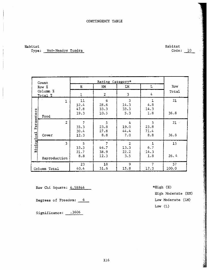
CONTINGENCY TABLE
Habitat Type: Wet'- Meadow Tundra
Count Rating Category* Row% H HM L.'1 Column % Total % 1 2 3
1 11 6 3 52.4 28 .,6 14.3
co 47.8 33.3 33.3 l-1 19.3 10.5 5.3 Q) ~ Food Q)
s \1j 2 7 5 4 l-1 \1j 33.3 23.8 19.0 p.,
o.-1 30.4 27.8 44.4 \1j Cover 12.3 8.8 7.0 C;j
-M
0 3 5 7 2 .-! 0 33.3 46.7 13.3 ...;
::0 21.7 38.9 22.2
I Reproduction 8.8 12.3 3.5
23 18 9 Column Total 40.4 31.6 15.8
Raw Chi Square: 6.58846
6 Degrees of Freedom: ---
Significance: .3606
116
L
4
1 4.8
14.3 1.8
5 23.8 71.4 8.8
1 6.7
14.3 1.8
7 12.3
Habitat Code: 10
Row
Total
21
36.8
21
36.8
15
26. 4
57 100.0
*High (H)
High Moderate (th'1)
Low Moderate (L'1)
Low (L)
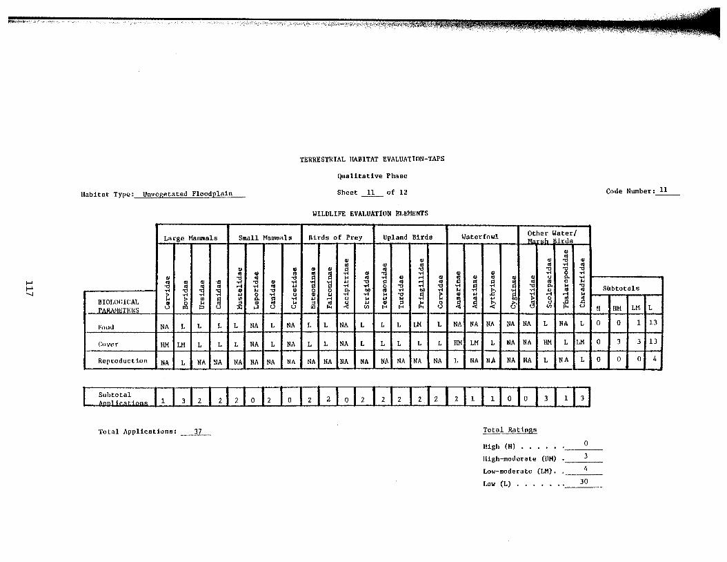
TERRESTRIAL IIABITA'f EVALUATION-TAPS
Qualitative Phase
Habitat Type: Unvegetated Floodplain Sheet of 12 Code Number: 11
WILDLIFE EVAI.UATION ELEMENTS
Large Mallllllals Small Mallllllall!:l Birds of Prey Upland Birds Waterfowl Other Water/ M• ·"h irds
QJ
QJ QJ Ill
QJ "tl QJ ol QJ Ill Ill ..-! Ill
QJ QJ QJ Ill ;! ol "tl "tl "tl "tl ol QJ <!l
~ ~ QJ "tl ..-! QJ QJ •rl 0 ·rl
QJ "tl Ill ~ ... Ill ..-! QJ ...... QJ ~ QJ ol QJ m CJ 0. ·rl <II
= QJ •41 ·.-1 "tl
= -a .... "tl p Ill :;:j 111 ~ ;! ol Ill 0 ... '<1 "' Ill ...... ..-! .... p ..-! ..-! 0 "tl "tl ..-! ;! "tl 0. ... "tl g!Jbtotals ..-! "' ~ ~ QJ 1-1 'tl QJ ~ 0 0. t>O Ill ..-! Ill) ..-! ... ·.-1 ~ :::l ~ <II "' ~ ..-! .... 0 ..-! CJ u ..-! ..-! 1-1 'tl p
~ QJ .... tt ...... 1-1
BIOLOGICAl. :> Ill ~ Ill 0. e ..-! .... ...... CJ 1-1 .... 1-1 ..-! ! Ill .... ~ 0 <II 11 Ill 0 :!:l ;.@ QJ 1-1 ;:) ~ <J .... QJ ;:) t: 0 !ii >. >. CJ .c PARM!Kl'l<:l{S u ~ u ...:1 u u ~ < til f-< f-< u < u 0 til 0. u I! liM LM. L
Food NA L L L L NA L NA L L NA L L L LM L NA NA NA NA NA L NA L 0 0 1 13
Cover 11M 1M L L L NA L NA L L NA L L L L L HM LM L NA NA 11M L LM 0 3 3 13
Reproduction NA L NA NA NA NA NA NA NA NA NA NA NA NA NA NA L NA NA NA NA L NA L 0 0 0 4
To tal Applications: ~--"'3.:..7_ Total Ratings
High (H) • • • 0
High-moderate (liM) 3
Low-moderate (LM). 4
Low (L) ••••••• __ Jo __
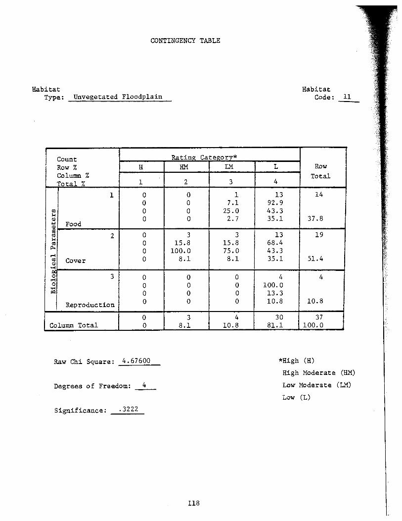
CONTINGENCY TABLE
Habitat Type: Unvegetated Floodplain
f Count Rating_ Category* Row % H HM L.'1
Column % Total % 1 2 3
1 0 0 1 0 0 7.1
co 0 0 25.0 ~ Q) 0 0 2.7 +.I Food Q)
6 0 3 3 ctl 2 ~ ctl 0 15.8 15.8
ll-< 0 100.0 75.0
I ..-1
0 8.1 8.1 ctl Cover C;l ~
~ 3 0 0 0 ..-! 0 0 0 0 ...-! ~ 0 0 0
Reproduction 0 0 0
0 3 4 Column Total 0 8.1 10.8
Raw Chi Square: 4.67600
Degrees of Freedom: 4
Significance: .3222
118
L
4
13 92.9 43.3 35.1
13 68.4 43.3 35.1
4 100.0 13.3 10.8
30 81.1
Habitat Code: 11
Row Total
14
37.8
19
51.4
4
10.8
37 100.0
*High (H)
High Moderate (HM)
Low MOderate (L'1)
Low (L)

TERRESTRIAL HABITAT EVALUATION-TAPS
Qualitative Phase
Uabitat T;ype: Agricultural Land Sheet _g_ of 12 Code Number._~--
WILDLIFE EVALUATION ELEMENTS
Large Mammals Small Mammals Birds of Prey Upland Birds Waterfowl Other Water/ M~ r<th Hrd
QJ
QJ QJ
., QJ "' QJ
<II QJ <II <II •rl <II Ill m Ill Ill .~
., :::l "' "' "' <II QJ
~ ~ QJ :::l ~ 111 .... 0 .... 111 "' <II "'
,.. ~ QJ .-! QJ QJ
~ 111 QJ <J p. .... ., 111 ~ =
.... "' Ill .... ·a ... p <II .-! <II .;] .~ ., <II <II 0
"" :::l <II .-! '" <II ... .... .... 0 "' .... "' .;] "' p.,
"" "' Subtotals "' "' 'tl QJ
"" "' QJ 0 0 p. 1>0 :1 •ri 1>0 '" "' ~ ~ ~ "' .,
~ '" .... .... ... 0 .... <J Ql u '" .... "' d ~ QJ .., a .-! "' BIOWGICAL > Ill ~ Ill p. c:l •rl .., .-! <J k 1.1 !; .... ~
<II ... 5 0 ~ ~ Ql 0 k :il QJ ~ ... ::1 <II <J .., QJ "' 0 !i! ~ :.... ()
PARAMETERS u ""' p u H u
""' "" < U') £-1 £-1 "" u u U') p., u H HM LM L
Food L L L NA L L L L L L L L L 1M HM L LM LM NA NA NA L NA L 0 1 3 15
Cover L L NA NA L 1 L L NA L NA L J, 1 LM L L L NA NA NA L NA L 0 0 1 15
Repro duet ion NA NA NA NA NA NA NA L NA NA NA NA NA NA L NA NA NA NA NA NA NA NA N/1 0 0 0 2
:::~~~:!ions I 2 I 211 I o I 21 2 12 I 3 11 I 2 I 1 I 2 I 2 I 2 13 I 2 I 21 2 I o I o I o I 2 I o 12 I
Total Applications: ---~ Total Ratings
High (H) • • •
High-moderate (liM)
Low-moderate (Uf).
!..ow (L) . • • • •
0
1
4
32 ------
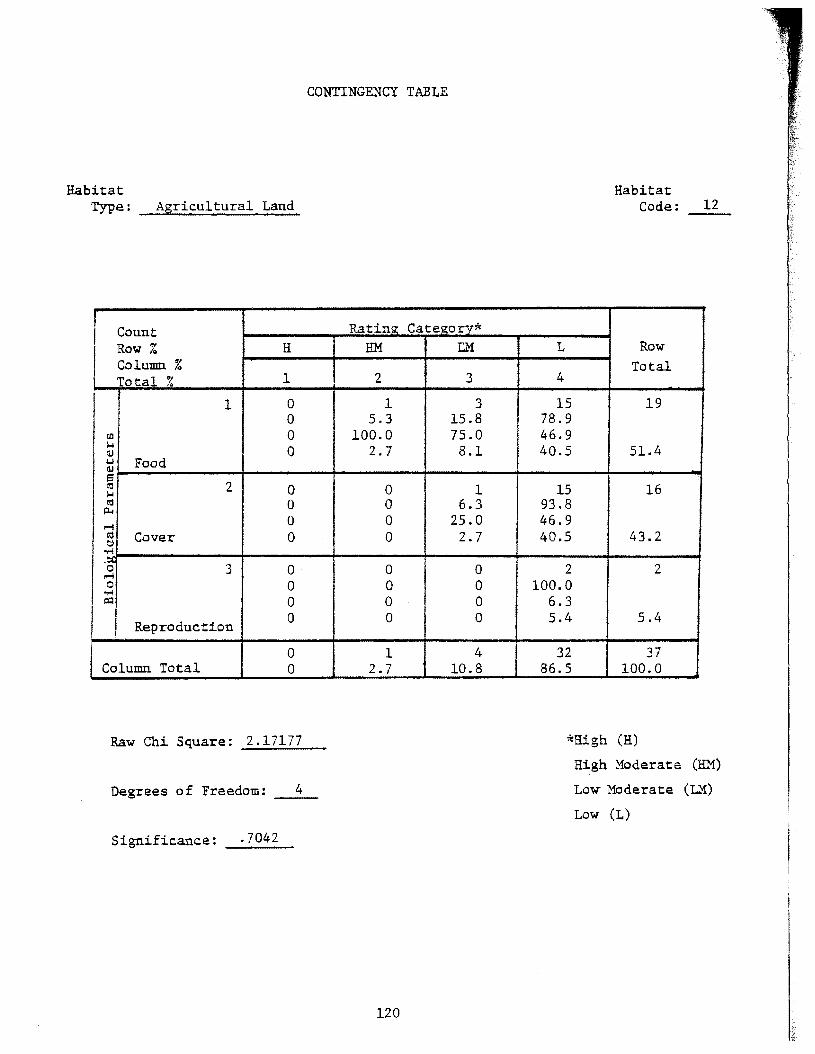
CONTINGENCY TABLE
Habitat Type: Agricultural Land
Count Rating Category* Row % H HM tM Column % Total % 1 2 3
1 0 1 3 0 5.3 15.8
c.Q 0 100.0 75.0 1-1 0 2.7 8.1 Q) .j,.\ Food Q)
~ 2 0 0 1 1-1 til 0 0 6.3 p.,.
1""'! 0 0 25.0
I til Cover 0 0 2.7 t;l ......
I '~ 3 0 0 0 0 ..-+ 0 0 0 0 ~ I:Q 0 0 0
l Reproduction 0 0 0
I Column Total 0 1 4 0 2.7 10.8
Raw Chi Square: 2.17177
Degrees of Freedom: _.....;4_
Significance: .7042
120
L
4
15 78.9 46.9 40.5
15 93.8 46.9 40.5
2 100.0
6.3 5.4
32 86.5
Habitat Code: 12
Row Total
19
51.4
16
43.2
2
5.4
37 100.0
*High (H)
High Moderate (HM)
Low MOderate (L~)
Low (L)
Appendix V: Plates
121
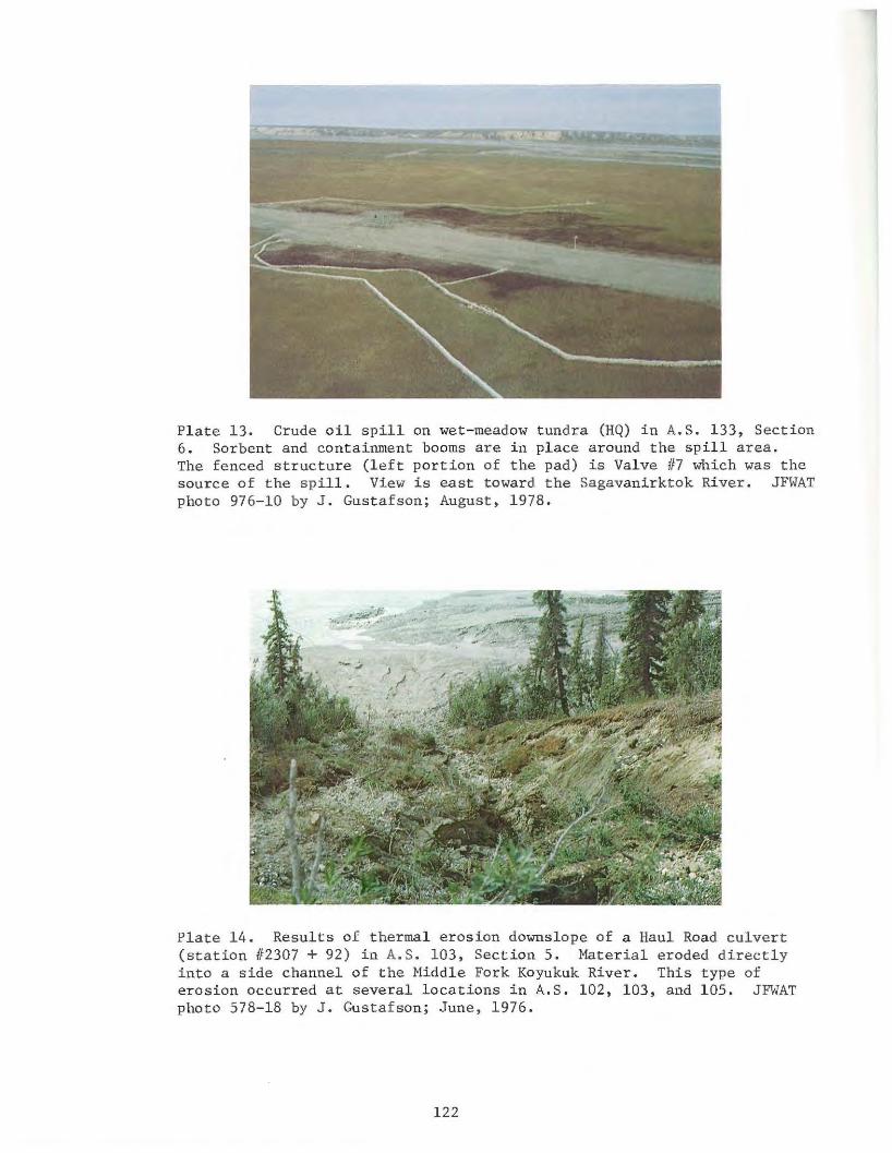
Plate 13. Crude oil spill on wet-meadow tundra (HQ) in A.S. 133, Section 6. Sorbent and containment booms are in place around the spill area. The fenced structure (left portion of t he pad) is Valve #7 which was the source of t he spill. View is east towar d the Sagavanirktok River. JFWAT photo 976-10 by J. Gustafson; August, 1978.
Plate 14. Results of thermal erosion downslope of a Haul Road culvert (station #2307 + 92) in A. S. 103, Section 5 . Material eroded directly into a side channel of the Middl e Fork Koyukuk River. This t ype of erosion occurred at several locations i n A.S. 102, 103, and 105. JFWAT pho t o 578-18 by J. Gust afson; June, 1976 .
122
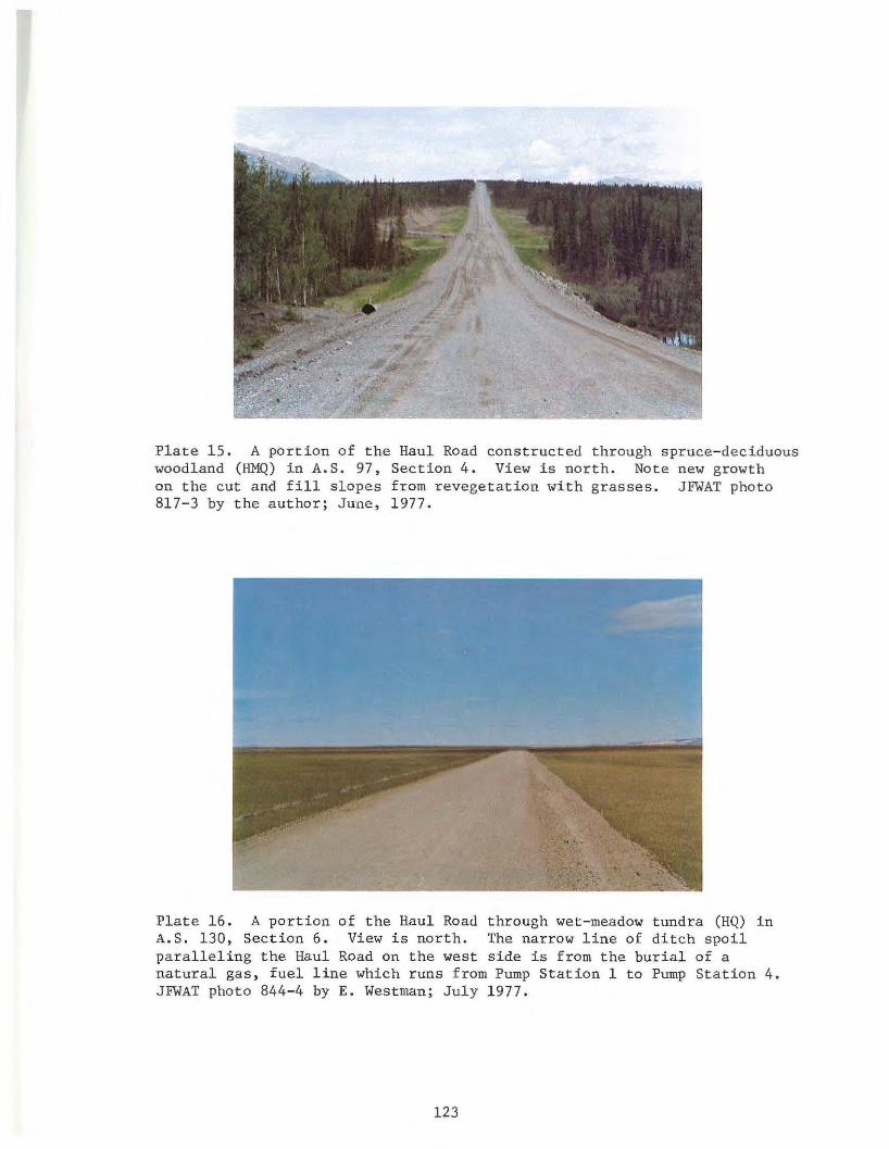
Plate 15. A portion of the Haul Road constructed through spruce-deciduous woodland (HMQ) in A.S. 97, Section 4. View is north. Note new growth on the cut and fill slopes from revegetation with grasses. JFWAT photo 817-3 by the author; June, 1977.
Plate 16. A portion of the Haul Road through wet-meadow tundra (HQ) in A.S . 130, Section 6 . View is north. The narrow line of ditch spoil paralleling the Haul Road on the west side is from the burial of a natural gas, fuel line which runs from Pump Station 1 to Pump Station 4. JFWAT photo 844-4 by E. Westman; July 1977.
123
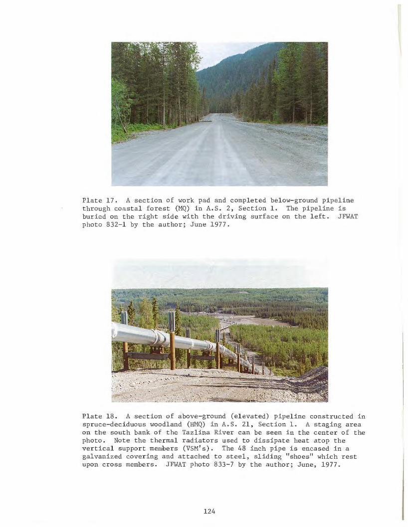
Plate 17. A section of work pad and completed below-ground pipeline through coastal forest (MQ) in A.S. 2, Section 1. The pipeline is buried on the right side 'vith the driving surface on the left. JFWAT photo 832-1 by the author; June 1977.
Plate 18. A section of above- ground (elevated) pipeline constructed in spruce-deciduous woodland (HMQ) in A. S. 21, Section 1. A staging area on the south bank of the Tazlina River can be seen in the center of the photo . Note the thermal radiators used to dissipate heat atop the vertical support members (VSM's). The 48 inch pipe is encased in a galvanized covering and attached to steel, sliding "shoes" which rest upon cross members. JFWAT photo 833-7 by the author; June, 1977.
124
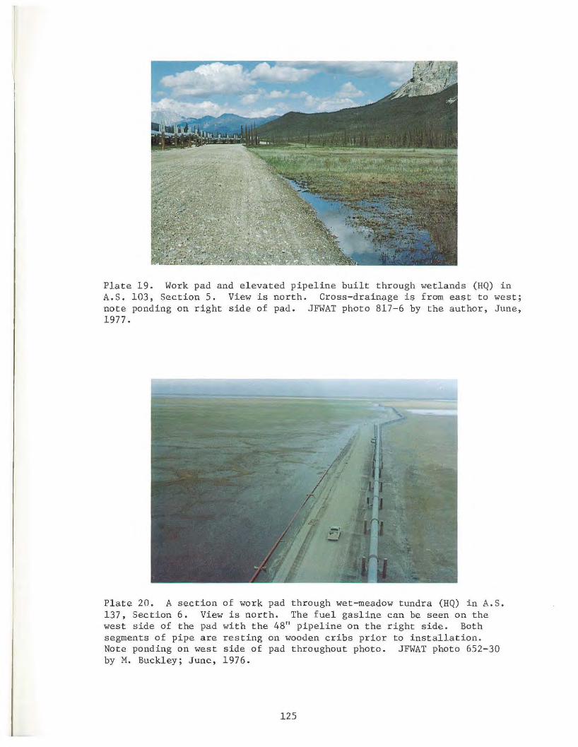
Plate 19. Work pad and elevated pipeline built through wetlands (HQ) in A.S . 103, Section 5. View is north. Cross- drainage is from east to west; note ponding on right side of pad. JFWAT photo 817- 6 by the author, June, 1977 .
Pl ate 20. A section of work pad through wet-meadow tundra (HQ) in A.S. 137, Section 6. Vi ew is north. The fuel gasline can be seen on the west side of the pad with the 48" pipeline on the right side. Both segments of pipe are resting on wooden cribs prior to installation. Note ponding on west side of pad throughout photo . JFWAT photo 652-30 by M. Buckl ey; June, 1976.
125
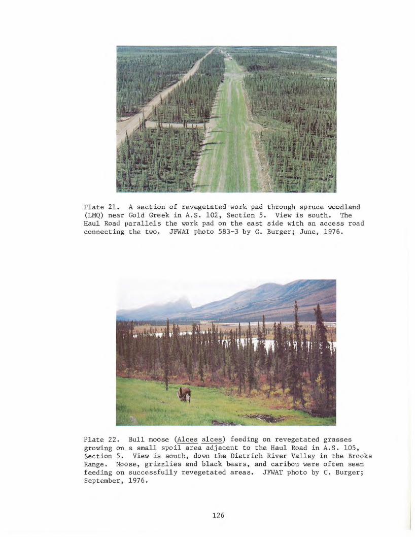
Plate 21. A section of revegetated work pad through spruce woodland (LMQ) near Gold Greek in A. S. 102, Section 5 . View is south. The Haul Road parallels the work pad on the east side with an access road connecting the two. JFWAT photo 583-3 by C. Burger; June, 1976.
Plate 22 . Bull moose (Alces alces) feeding on revegetated grasses growing on a small spoil area adjacent to the Haul Road in A. S. 105, Section 5. View is south, down the Dietrich River Valley in the Brooks Range. Moose, grizzlies and black bears, and caribou were often seen feeding on successfully revegetated areas. JFWAT photo by C. Burger; September, 1976.
126
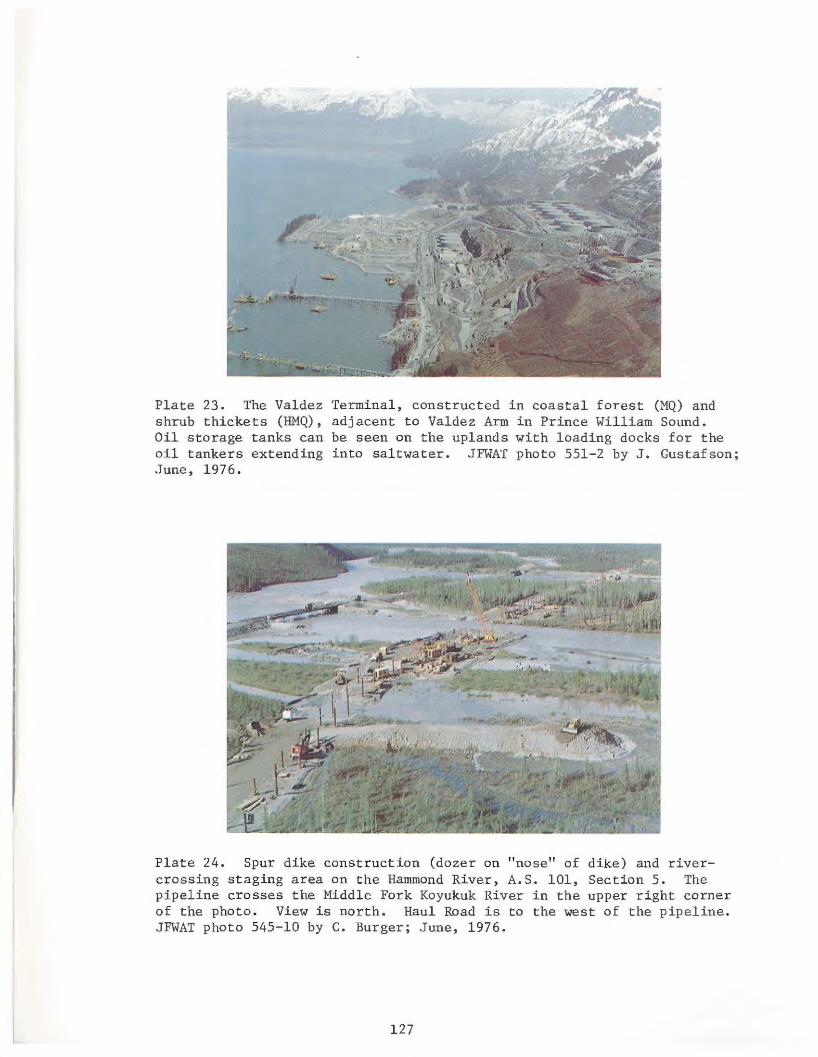
Plate 23. The Valdez Terminal, constructed in coastal forest (MQ) and shrub thickets (HMQ), adjacent to Valdez Arm in Prince William Sound. Oil storage tanks can be seen on the uplands with loading docks for the oil tankers extending into saltwater. JFWAT photo 551- 2 by J . Gustafson; June, 1976.
Plate 24. Spur dike construction (dozer on "nose" of dike) and rivercrossing staging area on the Hammond River, A.S . 101, Section 5. The pipeline crosses the Middle Fork Koyukuk River in the upper right corner of the photo. View is north. Haul Road is to the west of the pipeline. JFWAT photo 545-10 by C. Burger; June, 1976.
127
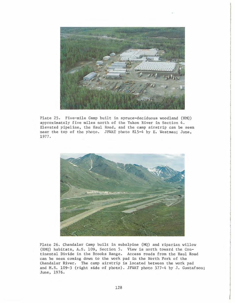
Plate 25. Five-mile Camp built in spruce-deciduous woodland (HMQ) approximat ely five miles north of the Yukon River in Section 4 . Elevated pipeline, the Haul Road, and the camp airstrip can be seen near the top of the photo. JFWAT photo 815-4 by E. Westman; June, 1977.
Plate 26. Chandalar Camp built in subalpine (MQ) and riparian willow (HMQ) habitats, A.S. 109, Section 5 . View is north toward the Continental Divide in the Brooks Range. Access roads from the Haul Road can be seen coming down to the work pad in the North Fork of the Chandalar River. The camp airstrip is located between the work pad and M. S. 109- 3 (right side of photo). JFWAT photo 577-4 by J . Gustafson; June, 1976.
128
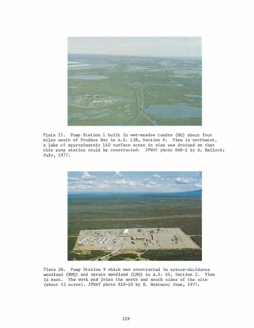
Plate 27. Pump Station 1 built in wet- meadow tundra (HQ) about four miles south of Prudhoe Bay in A.S . 138, Sect ion 6. View is northwest. A lake of approximately 140 surface acres in size was drained so that this pump station could be constructed. JFWAT photo 868- 1 by R. Hall ock; July , 1977.
Plate 28. Pump St ation 9 which was constructed in spruce-deciduous woodland (HMQ) and spruce woodl and (LMQ) i n A.S. 44, Sec t ion 2 . View is east. The work pad j oins the north and south s i des of the site (about 43 acres) . JFWAT photo 818-10 by E. Westman; June, 1977 .
129
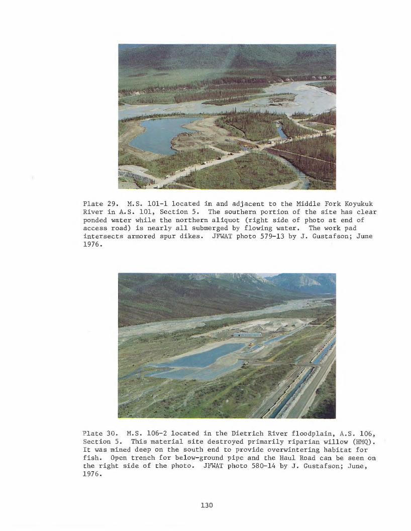
Plate 29. M.S. 101-1 located in and adjacent to the Middle Fork Koyukuk River in A.S. 101, Section 5. The southern portion of the site has clear ponded water while the northern aliquot (right side of photo at end of access road) is nearly all submerged by f l owing water. The work pad intersects armored spur dikes . JFWAT photo 579-13 by J. Gustafson; June 1976.
Plate 30. M.S. 106-2 located i n the Dietrich River floodplain, A. S. 106, Section 5. This material site destroyed pr i marily riparian willow (HMQ). It was mined deep on the south end to provide overwintering habitat for fish. Open trench for below-ground pipe and the Haul Road can be seen on the right side of the photo. JFWAT photo 580-14 by J. Gustafson; June, 1976.
130
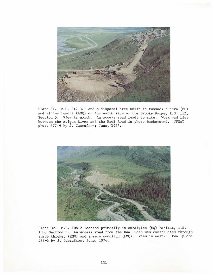
M.S. 112-3.1 and a disposal area built in tussock tundra (MQ) tundra (LMQ) on the north side of the Brooks Range, A.S. 112, View is north. An access road leads to site. Work pad lies Atigun River and the Haul Road in photo background. JFWAT by J. Gustafson; June, 1976.
Plate 31. and alpine Section 5 . between the photo 577 -9
Plate 32. M.S. 108-2 located primarily in subalpine (MQ) habitat, A. S. 108, Section 5. An access road from the Haul Road was constructed through shrub thicket (HMQ) and spruce woodland (LMQ). View is west. JFWAT photo 577 - 3 by J. Gustafson; June, 1976.
131
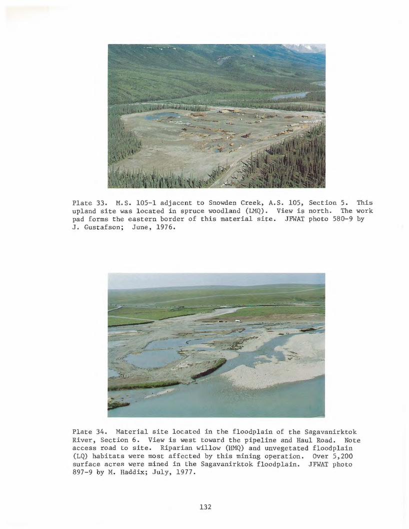
Plate 33. M.S . 105- 1 adjacent to Snowden Creek, A. S. 105, Section 5 . This upland site was located in spruce woodland (LMQ). View is north. The work pad forms the eastern border of this material site . JFWAT photo 580- 9 by J . Gustafson; June, 1976.
Plate 34 . Material site located in the floodplain of the Sagavanirktok River , Section 6 . View is west toward the pipeline and Haul Road. Note access road to site. Riparian willow (HMQ) and unvegetated floodplain (LQ) habitats were most affected by this mini ng operation. Over 5,200 surface acres were mined in the Sagavanirktok floodplain. JFWAT photo 897-9 by M. Haddix ; July, 1977 .
132