CONSTRUCTION OF A LOW TEMPERATURE SIMPLIFIED …

CONSTRUCTION OF A LOW TEMPERATURE SIMPLIFIED

PSYCHROMETRIC CHART

Technical Report

Submitted in partial fulfilment of the requirements for the course of

Design of Air Conditioning Systems (TH819)

in

Mechanical Engineering

By

Sthavishtha B.R.

(13ME125)

Under the supervision of

Prof. T.P. Ashok Babu

(Dean Faculty Welfare)

DEPARTMENT OF MECHANICAL ENGINEERING

NATIONAL INSTITUTE OF TECHNOLOGY KARNATAKA

SURATHKAL, MANGALORE - 575025 (INDIA)

April, 2017

ACKNOWLEDGEMENT

I am deeply indebted to Prof. T.P. Ashok Babu for guiding me throughout the course of this

work. Without his support and motivation, this work would not have been successful enough

to be completed within the stipulated time.

Finally, I am thankful to the Almighty for showering his blessings, thus enabling me to

complete this course and its project work satisfactorily.

NOMENCLATURE

𝑝 Partial pressure (𝑁

𝑚2)

𝑅𝐻 Relative Humidity

𝑤 Specific Humidity (𝑘𝑔 /𝑘𝑔 )

𝑕 Enthalpy (𝑘𝐽 /𝑘𝑔 )

t Dry bulb temperature (°C)

Σ Sigma heat function

𝑅 Gas constant (𝑘𝐽 /𝑘𝑔𝐾)

T Temperature (K)

Subscripts

a Dry air

atm Atmospheric

v Vapour

s Saturated

f Saturated water (specifically for enthalpy)

Superscript

*

Saturated conditions (during adiabatic saturation)

ABSTRACT

The current study attempts to construct a low temperature psychrometric chart whose dry

bulb temperature varies from -60 °C to 0 °C at constant atmospheric pressure. For this

purpose, a numerical code was developed in MATLAB and the required thermodynamic data

was imported from a file. The constructed chart has also been validated with an available low

temperature psychrometric chart (in the reference section), which satisfies the credibility of

the developed code and the method. In the future, this code can be extended to construct

charts operating in other vapour systems or at other altitudes with sufficient accuracy. This

report also contains the methodology required to construct the psychrometric chart along with

the MATLAB numerical code for reference.

TABLE OF CONTENTS

1 INTRODUCTION .............................................................................................................. 7

1.1 Overview of Psychrometrics and Psychrometric Chart .............................................. 7

1.2 Motivation ................................................................................................................... 7

1.3 Literature Review ........................................................................................................ 7

1.4 Psychrometric Relations .............................................................................................. 7

2 METHODOLOGY ............................................................................................................. 9

2.1 Saturation Line ............................................................................................................ 9

2.2 Constant Relative Humidity Lines ............................................................................ 10

2.3 Constant Specific Volume Lines ............................................................................... 11

2.4 Constant Thermodynamic Wet Bulb Temperature Lines ......................................... 11

2.5 Constant Enthalpy lines ............................................................................................. 12

2.6 Sensible Heat Factor (SHF) Protractor...................................................................... 13

3 RESULTS AND DISCUSSIONS .................................................................................... 14

3.1 Psychrometry chart from the current study ............................................................... 14

3.2 Validation of the Chart obtained from the present study .......................................... 14

3.3 Comparison of Saturation water Vapour Pressure with data from ASHRAE [9] and

correlation [9, 12] ................................................................................................................. 16

4 NUMERICAL CODE....................................................................................................... 18

5 CONCLUSIONS .............................................................................................................. 26

6 APPENDIX ...................................................................................................................... 27

6.1 Thermodynamic Data from ASHRAE [9] ................................................................ 27

6.2 Percentage Deviations of the psychrometric values obtained along constant enthalpy

lines on comparison with reference chart [11] and ASHRAE table [9] ............................... 28

6.3 Percentage Deviation of saturated water vapour pressure between the ones from

ASHRAE [9] and correlation [9,12] .................................................................................... 29

7 REFERENCES ................................................................................................................. 31

LIST OF FIGURES

Figure 2.1. Plot of saturation line in the psychrometric chart .................................................. 10

Figure 2.2. Plot of constant relative humidity lines in the psychrometric chart ...................... 10

Figure 2.3. Plot of constant specific volume lines in the psychrometric chart ........................ 11

Figure 2.4. Plot of constant wet bulb temperature lines in the psychrometric chart ................ 12

Figure 2.5. Constant enthalpy lines in the psychrometric chart ............................................... 13

Figure 3.2. Validation of the constant specific volume line from the current study with

reference chart [11] .................................................................................................................. 14

Figure 3.1. Low temperature simplified psychrometric chart obtained from the present study

.................................................................................................................................................. 15

Figure 3.3. Validation of the constant enthalpy line from the current study with the reference

chart [11] .................................................................................................................................. 16

1 INTRODUCTION

1.1 Overview of Psychrometrics and Psychrometric Chart Psychrometrics is a subject which deals with the determination of thermodynamic properties

of gas-vapour mixtures. A psychrometric chart helps in graphically representing these

properties and enables a lay man to easily identify them without explicitly calculating them

from the tables given in several data handbooks. The most commonly used psychrometric

charts deal with air-water vapour (or moist air) systems.

Psychrometric charts have numerous applications. They can be used for analyzing the

psychrometric processes involving moist air and in determination of human thermal comfort

conditions. Additionally, the properties of moist air listed in the psychrometric chart make it

imperative to design air-conditioning equipments for storage of food, dryers and cooling

towers in food processing plants [1].

Several standard psychrometric charts are available by ASHRAE for reference [2,9]. These

are constructed at different altitudes (different pressures) and for a range of dry bulb

temperatures (low, high, normal and very high). In this direction, generalized psyhcrometric

charts [3] and charts at different gas-vapour systems [4,5] have also been constructed.

1.2 Motivation

In polar regions and harsh climatic areas, the dry bulb temperatures may drop way below the

freezing point of water (0°C). Hence, in such cases, it becomes vital for constructing a low

temperature psychrometric chart. Moreover, manual construction of a psychrometric chart

helps the students in improving their fundamental understanding of thermodynamic relations

and psychrometric processes [6]. With this motivation, the current study aims to plot the

psychrometric chart from -60°C to 0°C dry bulb temperature at atmospheric pressure.

1.3 Literature Review

Plethora of previous works in constructing psychometric charts and tutorials have been

carried out [3,4,5,6,7]. Most of these charts have been constructed using Flash, HTML pages

or Excel spreadsheets. However, the current study attempts to construct a psychrometric chart

by programming in MATLAB R2013, wherein the saturated properties of moist air are

imported from excel files.

1.4 Psychrometric Relations The psychrometric relations used in the current study are taken from [8,9]. Some of them

necessary for plotting the chart are summarized below.

𝑃𝑎𝑟𝑡𝑖𝑎𝑙 𝑃𝑟𝑒𝑠𝑠𝑢𝑟𝑒 𝑜𝑓 𝑑𝑟𝑦 𝑎𝑖𝑟 (

𝑁

𝑚2): 𝑝𝑎 = 𝑝𝑎𝑡𝑚 − 𝑝𝑣 (1)

𝑅𝑒𝑙𝑎𝑡𝑖𝑣𝑒 𝐻𝑢𝑚𝑖𝑑𝑖𝑡𝑦: 𝑅𝐻 = 𝑝𝑣

𝑝𝑠 (2)

𝑆𝑝𝑒𝑐𝑖𝑓𝑖𝑐 𝐻𝑢𝑚𝑖𝑑𝑖𝑡𝑦(𝑘𝑔 /𝑘𝑔 ) ∶ 𝑤 = 0.62198 𝑝𝑣

𝑝𝑎

(3)

𝑆𝑝𝑒𝑐𝑖𝑓𝑖𝑐 𝑉𝑜𝑙𝑢𝑚𝑒(𝑚3 /𝑘𝑔 ) ∶ 𝑣𝑎 = 𝑅𝑎𝑇

𝑝𝑎

(4)

𝑆𝑝𝑒𝑐𝑖𝑓𝑖𝑐 𝐻𝑢𝑚𝑖𝑑𝑖𝑡𝑦 𝑎𝑡 𝑠𝑎𝑡𝑢𝑟𝑎𝑡𝑖𝑜𝑛(𝑘𝑔 /𝑘𝑔 ) ∶ 𝑤𝑠 = 0.62198 𝑝𝑠

𝑝𝑎 (5)

𝐸𝑛𝑡𝑕𝑎𝑙𝑝𝑦 (𝑘𝐽 /𝑘𝑔 ) ∶ 𝑕 = 1.006 + 1.805𝜔 𝑡 + 2501𝜔

(6)

2 METHODOLOGY

This chapter lists down the relevant method adopted to construct the low temperature

psychrometric chart. The procedure for constructing the psychrometric chart follows [8]. The

table containing the thermodynamic properties of moist air are taken from [9], which is also

available in the Appendix. Unlike [10] which uses Virial equation of states to determine the

specific volume of moist air, this study directly imports the data present from the excel file,

which is fairly simple and accurate.

All psychrometric properties of moist air can be determined when any three properties are

known. Since the psychrometric chart is constructed at constant atmospheric pressure, any

two independent variables in the psychrometric chart can help one in locating other properties

too. This is the basic principle adopted in the current study.

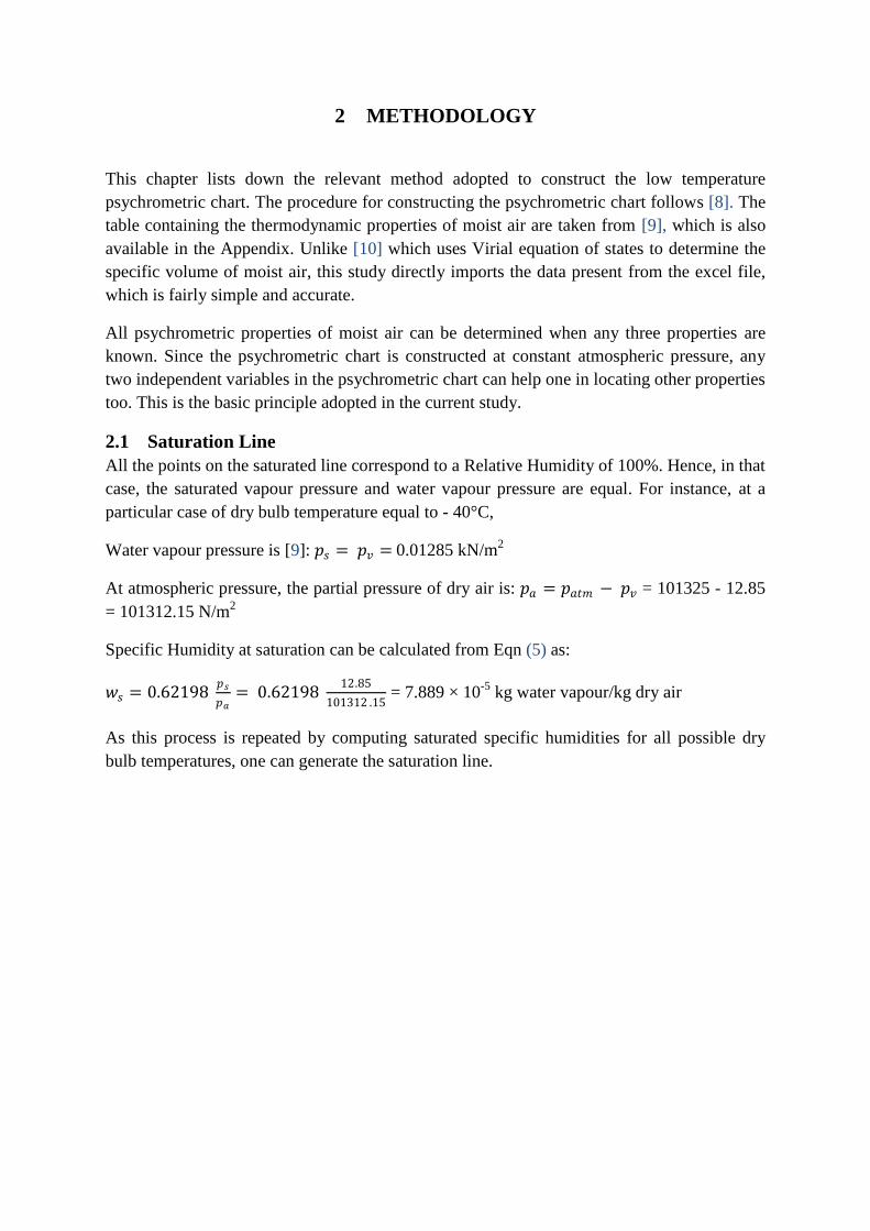
2.1 Saturation Line

All the points on the saturated line correspond to a Relative Humidity of 100%. Hence, in that

case, the saturated vapour pressure and water vapour pressure are equal. For instance, at a

particular case of dry bulb temperature equal to - 40°C,

Water vapour pressure is [9]: 𝑝𝑠 = 𝑝𝑣 = 0.01285 kN/m2

At atmospheric pressure, the partial pressure of dry air is: 𝑝𝑎 = 𝑝𝑎𝑡𝑚 − 𝑝𝑣 = 101325 - 12.85

= 101312.15 N/m2

Specific Humidity at saturation can be calculated from Eqn (5) as:

𝑤𝑠 = 0.62198 𝑝𝑠

𝑝𝑎= 0.62198

12.85

101312 .15 = 7.889 × 10

-5 kg water vapour/kg dry air

As this process is repeated by computing saturated specific humidities for all possible dry

bulb temperatures, one can generate the saturation line.

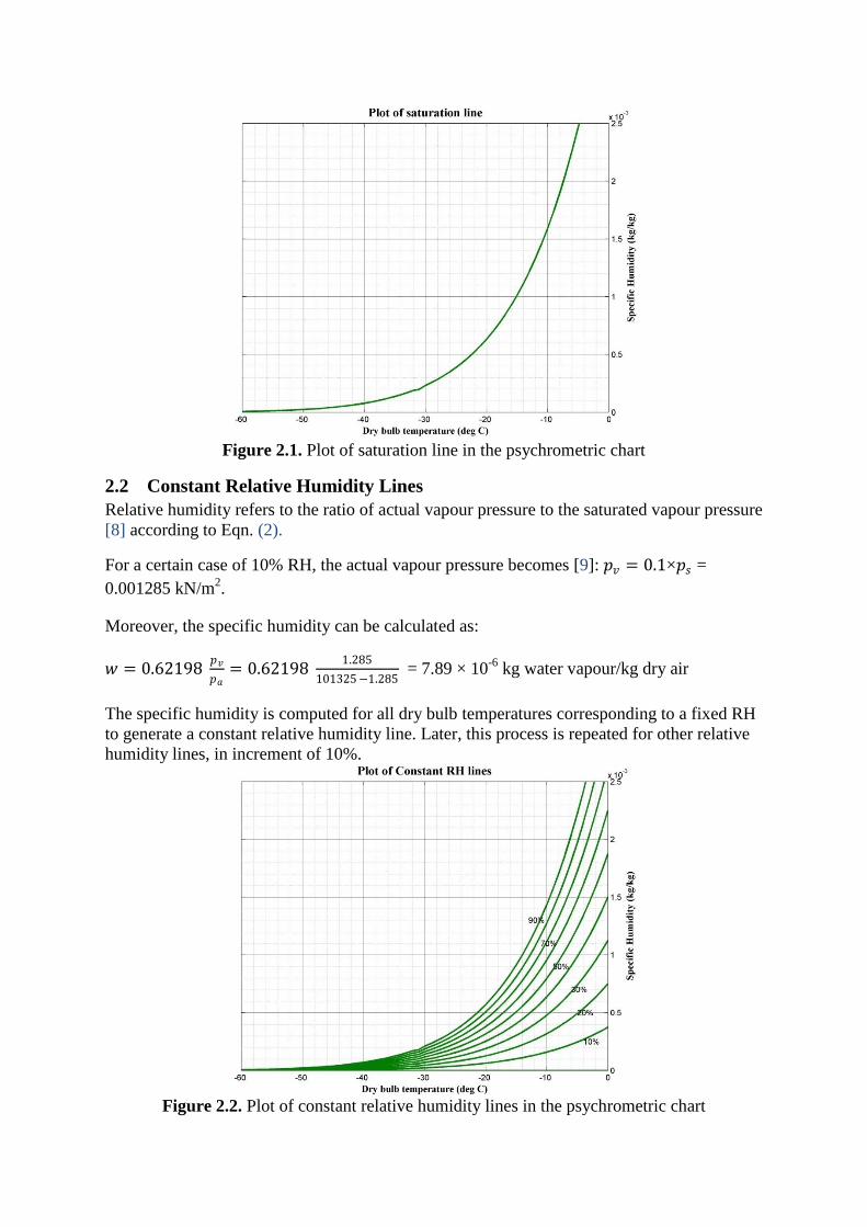
Figure 2.1. Plot of saturation line in the psychrometric chart

2.2 Constant Relative Humidity Lines

Relative humidity refers to the ratio of actual vapour pressure to the saturated vapour pressure

[8] according to Eqn. (2).

For a certain case of 10% RH, the actual vapour pressure becomes [9]: 𝑝𝑣 = 0.1×𝑝𝑠 =

0.001285 kN/m2.

Moreover, the specific humidity can be calculated as:

𝑤 = 0.62198 𝑝𝑣

𝑝𝑎= 0.62198

1.285

101325 −1.285 = 7.89 × 10

-6 kg water vapour/kg dry air

The specific humidity is computed for all dry bulb temperatures corresponding to a fixed RH

to generate a constant relative humidity line. Later, this process is repeated for other relative

humidity lines, in increment of 10%.

Figure 2.2. Plot of constant relative humidity lines in the psychrometric chart

2.3 Constant Specific Volume Lines

For this task, an iterative procedure [8] was adopted to compute specific volume and its

corresponding saturated dry bulb temperature. For a fixed specific volume, an approximate

saturated dry bulb temperature and its corresponding saturation pressure were estimated by

interpolation from the data in the excel file. The specific volume (approximate) was later

computed according to Eqn. (4):

𝑣𝑎 = 𝑅𝑎𝑇

𝑝𝑎=

287.1 × (273.15 + 𝑡)

101325 − (1000 × 𝑝𝑠)

The error between the approximate and fixed specific volume was calculated for the iteration

to proceed. In the developed numerical code, the error (absolute) was fixed to be 3×10-6

according to the user convenience. Moreover, the dry bulb temperature was incremented

(decremented) when the approximate specific volume came out to be more than the fixed

specific volume (vice-versa). Later, the saturated specific humidity and the dry bulb

temperature lying on the fixed volume line at zero humidity was calculated. This process was

later repeated for plotting other constant specific volume lines.

Figure 2.3. Plot of constant specific volume lines in the psychrometric chart

2.4 Constant Thermodynamic Wet Bulb Temperature Lines

The constant wet bulb temperature corresponds to the process of adiabatic saturation,

Σ = 𝑕 − 𝜔𝑕𝑓∗ = 𝑕∗ − 𝜔∗𝑕𝑓

∗ = Σ∗ = constant

where the ∗ superscript corresponds to the saturated conditions. For instance, at a specific dry

bulb temperature of - 40 °C, saturated specific humidity [9] is 7.889 × 10-5

kg water

vapour/kg dry air. To calculate the saturated enthalpy, we use the Eqn. (6):

𝑕∗ = 1.006 + 1.805𝜔∗ 𝑡∗ + 2501𝜔∗

Later, Σ = 𝑕∗ − 𝜔∗𝑕𝑓∗ is calculated.

Since the constant wet bulb temperature line is a line with constant slope, the temperature

corresponding to zero specific humidity lying along this line is computed as per Eqn. (7).

This was later joined to the saturated dry bulb temperature to get a straight line.

𝑡 = Σ

1.006

(7)

Figure 2.4. Plot of constant wet bulb temperature lines in the psychrometric chart

2.5 Constant Enthalpy lines

Rather than plotting enthalpy deviation lines on the chart, separate enthalpy lines were drawn.

For a fixed enthalpy, the dry bulb temperature corresponding to zero specific humidity was

estimated by Eqn. (7).

For enhancing the readability of the constant enthalpy lines, an enthalpy axis is essential. For

user convenience, the enthalpy axis here is drawn as a straight line with a slope of 4.5 × 10-5

,

which extends as a straight line joining the corner points of the plot space : (-60, 0.25×10-3

)

and (-10,2.5×10-3

). The equation of the line joining these corner points can be calculated to

be:

𝑤 = 4.5 × 10−5t + 2.95 × 10−3 kg/kg.

(8)

Substituting the expression for w from Eqn. (8) in Eqn. (6) and simplifying, we get

𝑕 = 9.025 × 10−5t2 + 1.1373𝑡 + 8.7535 𝑘𝐽/𝑘𝑔

(9)

For a fixed enthalpy, this quadratic equation is solved to determine the dry bulb temperature

which lies on the enthalpy axis. Finally, a line joining this temperature to the dry bulb

temperature at zero specific humidity gives a straight line corresponding to constant enthalpy.

Figure 2.5. Constant enthalpy lines in the psychrometric chart

2.6 Sensible Heat Factor (SHF) Protractor

The protractor at the top left of the psychrometric chart is the SHF protractor. SHF is defined

as the ratio of the sensible heat to total heat transfer. The presence of a protractor is necessary

to identify the direction and slope of the moist air process line. For plotting SHF lines, the

procedure available in [8] has been adopted.

3 RESULTS AND DISCUSSIONS

3.1 Psychrometry chart from the current study

Using the aforementioned psychrometric equations along with the methodology (previous

chapter) to plot the psychrometric curves, a numerical code had been developed in MATLAB

R2013 to plot the psychrometric chart from 0 to -60°C dry bulb temperature at constant

atmospheric pressure of 1 atm. The relevant thermodynamic data was imported from an excel

file (also found in the Appendix). The psychrometric chart obtained from the current study is

shown Fig.3.1. This chart resembles the commercial one present in [11], and is validated as

described later which establishes the credibility of the developed code and reliability of the

present chart for educational purposes.

3.2 Validation of the Chart obtained from the present study

The procedure of validation is inherent for every numerical code and method. Hence, to

render the credibility of the established code and its developed chart, validation of specific

volume lines (at 0.76 m3/kg) and enthalpy lines (at -20 kJ/kg) has been performed with the

data points extracted from the reference chart [11]. The data points and the lines in Figs. 3.2

and 3.3 are quite close to each other, thus confirming the validity of the present study.

Figure 3.1. Validation of the constant specific volume line from the current study with

reference chart [11]

Figure 3.2. Low temperature simplified psychrometric chart obtained from the present study

Figure 3.3. Validation of the constant enthalpy line from the current study with the reference

chart [11]

For a detailed analysis of the psychrometric values obtained from the current study, they have

been compared with the values extracted from the reference chart [11] by calculating the

percentage deviations at constant specific enthalpy lines over the entire dry bulb temperature

range. This will allow the reader or the user to obtain the psychrometric values from this

chart with an uncertainty range.

The percentage deviations over the range of the chart along constant enthalpy lines can be

found in Appendix 6.2 and Psychro_Chart_Deviations excel file, which can be found in

Folder 4 - Matlab files and Program_corrections_20-04-2017. As a consequence of this

validation study, the values were found to lie within an absolute deviation of 0.555% to

2.455% in comparison to the reference chart [11], which deems the current study to be

accurate. Since the available reference chart [11] extends up to a dry bulb temperature of -50

°C, all deviations of the chart from the current study have thus been studied till this

temperature. However, the specific enthalpy of dry air from this chart has been compared

with the data in ASHRAE [6] to render credibility to the validation study over the entire low

temperature range. Thus, the chart obtained from the current study is equally accurate as

existing commercial charts, with an uncertainty of less than 2.455 %.

3.3 Comparison of Saturation water Vapour Pressure with data from ASHRAE

[9] and correlation [9, 12]

A numerical code was developed in MATLAB (available in Chapter 4 - Numerical Code) to

compute the saturated vapour pressure values from this correlation, which was later

compared with ASHRAE data [9] (also in Appendix).

The correlation available for calculating the saturation water vapour pressure at low

temperatures ranging from -100 to 0 °C can be given by [9,12] :

𝑙𝑛𝑝𝑠 =𝐶1

𝑇+ 𝐶2 + 𝐶3𝑇 + 𝐶4𝑇

2 + 𝐶5𝑇3 + 𝐶6𝑇

4 + 𝐶7𝑙𝑛𝑇 (10)

where

𝐶1 = -5.6745359 × 103

𝐶2 = 6.3925247

𝐶3 = -9.677843 × 10-3

𝐶4 = 6.2215701 × 10-7

𝐶5 = 2.0747825 × 10-9

𝐶6 = -9.484024 × 10-13

𝐶7 = 4.1635019

Comparison between these values (from Appendix 6.3) shows excellent agreement of the

correlation values with accurate ASHRAE data, with an absolute deviation lying between

0.000213 % to 0.307013 %. This infers that this correlation is reliable, which will render

simple computations over importing the data from tables (ASHRAE) to the program. This

could also be used when the range of dry bulb temperatures are huge to be imported from

tables.

4 NUMERICAL CODE

Contruction_Psychor_chart_MATLAB.m

The numerical code developed in MATLAB to generate the psychrometric chart is shown

below. The line colours, line widths and additional text were added on the plot to make it user

friendly. Comments are also shown to explain the significance of each line in the code.

%Program to plot a low temperature simplified psychrometric chart %% Section to plot the saturation line of 100% RH clc; clear all; format long prop=xlsread('Thermodynamic prop.xlsx'); %reading thermodynamic properties

from excel file t_a=prop(:,1); %dry bulb temperature (deg C) p_s=prop(:,2); %saturated vapour pressure (kN/m^2) v_sp=prop(:,3); %specific volume of moist air (m^3/kg) h_f=prop(:,4); %enthalpy of saturated water (kJ/kg) w_s=(0.62198*p_s*1000)/(101325-(1000*p_s)); %saturated specific humidity w_s=w_s(:,1); figure(1); plot(t_a,w_s,'Color',[0 0.5 0],'LineWidth',2); %plotting saturation line of

100% RH - Green grid on; grid minor; axis([-60 0 0 2.5e-3]); xlabel('Dry bulb temperature (deg C)','FontSize',12,'FontName','Times New

Roman','FontWeight','bold'); ylabel('Specific Humidity (kg/kg)','FontSize',12,'FontName','Times New

Roman','FontWeight','bold'); set(gca,'yaxislocation','right'); title('Plot of saturation line','FontSize',15,'FontName','Times New

Roman','FontWeight','bold'); print(figure(1),'Saturation_Line','-djpeg','-r300'); figure(6); % figure('units','inches'); % set(gcf,'pos',[1 1 1366 608]) fullfig(figure(6)); plot(t_a,w_s,'Color',[0 0.5 0],'LineWidth',2); %plotting saturation line of

100% RH - Green hold on; %holds the figure for plotting next portions grid on; %plotting grid lines grid minor; xlabel('Dry bulb temperature (deg C)','FontSize',12,'FontName','Times New

Roman','FontWeight','bold'); ylabel('Specific Humidity (kg/kg)','FontSize',12,'FontName','Times New

Roman','FontWeight','bold'); set(gca,'yaxislocation','right'); title('Psychrometric chart','FontSize',15,'FontName','Times New

Roman','FontWeight','bold'); axis([-65 0 0 2.5e-3]); %limits of x- and y-axis

%% Section to plot constant RH lines for rh=0.1:0.1:0.9 %varying rh from 10% to 90% p_v=rh*p_s; %vapour pressure w=(0.62198*p_v*1000)/(101325-(1000*p_v)); %specific humidity at a

constant RH

figure(2); plot(t_a,w,'g-','Color',[0 0.5 0],'LineWidth',2); %plotting constant RH

lines from 10% to 90% RH - Green grid on; grid minor; axis([-60 0 0 2.5e-3]); xlabel('Dry bulb temperature (deg C)','FontSize',12,'FontName','Times

New Roman','FontWeight','bold'); ylabel('Specific Humidity (kg/kg)','FontSize',12,'FontName','Times New

Roman','FontWeight','bold'); set(gca,'yaxislocation','right'); title('Plot of Constant RH lines','FontSize',15,'FontName','Times New

Roman','FontWeight','bold'); hold on; figure(6); plot(t_a,w,'g-','Color',[0 0.5 0]); %plotting constant RH lines from

10% to 90% RH - Green grid on; grid minor; hold on; end figure(2); text(-4,0.25e-3,'10%'); text(-5,0.5e-3,'20%'); text(-6,0.7e-3,'30%'); text(-9,0.9e-3,'50%'); text(-11,1.1e-3,'70%'); text(-13,1.3e-3,'90%'); print(figure(2),'Constant RH lines','-djpeg','-r300'); figure(6); text(-4,0.25e-3,'10%','Color',[0 0.5 0]); text(-5,0.5e-3,'20%','Color',[0 0.5 0]); text(-6,0.7e-3,'30%','Color',[0 0.5 0]); text(-9,0.9e-3,'50%','Color',[0 0.5 0]); text(-11,1.1e-3,'70%','Color',[0 0.5 0]); text(-12,1.3e-3,'90%','Color',[0 0.5 0]); %% Section to plot constant volume lines %adopting an iterative procedure for v_sq=0.61:0.01:0.77 %varying vol. from 0.61 m^3/kg to 0.77 m^3/kg t_s0=interp1(v_sp,t_a,v_sq); %guessed (interpolated) value of satd.

temp diff=1.0; %assumed difference while diff>3e-6 p_s0=interp1(t_a,p_s,t_s0); %value of satd. pressure at that satd.

temp (interpolated) v_s0=(287.1*(t_s0+273.15))/(101325-(1000*p_s0)); %recalc. sp.

volume diff=abs(v_s0-v_sq); %absolute error b/w true sp. volume and

approx. one if diff<3e-6 break; elseif v_s0>v_sq t_s0=t_s0-0.001; %decrementing satd. temp continue; else t_s0=t_s0+0.001; %incrementing satd. temp continue; %continues the loop end end w_sp=0.62198*(1000*p_s0)/(101325-(1000*p_s0)); %satd. humidity at

const. volume

t_0=(101325*v_sq)/287.3-273.15; %temp at 0 humidity along the const.

sp. volume line figure(3); plot([t_s0,t_0],[w_sp,0],'b-','LineWidth',2); %plotting constant volume

lines grid on; grid minor; axis([-60 0 0 3.5e-3]); xlabel('Dry bulb temperature (deg C)','FontSize',12,'FontName','Times


Roman','FontWeight','bold'); set(gca,'yaxislocation','right'); title('Plot of Constant specific volume

lines','FontSize',15,'FontName','Times New Roman','FontWeight','bold'); hold on; figure(6); plot([t_s0,t_0],[w_sp,0],'b-','LineWidth',2); %plotting constant volume

lines hold on; grid on; grid minor; end figure(3); text(-6,3.1e-3,'0.77 m^3/kg'); text(-7,2.5e-3,'0.76 m^3/kg'); text(-11,2e-3,'0.75 m^3/kg'); text(-14,1.4e-3,'0.74 m^3/kg'); text(-18,1e-3,'0.73 m^3/kg'); text(-25,0.5e-3,'0.71 m^3/kg'); text(-32,0.4e-3,'0.69 m^3/kg'); text(-40,0.2e-3,'0.67 m^3/kg'); text(-46,0.1e-3,'0.65 m^3/kg'); text(-58,0.08e-3,'0.61 m^3/kg'); print(figure(3),'Constant specific volume lines','-djpeg','-r300'); figure(6); text(-3,2e-3,'0.77 m^3/kg','rotation',90,'Color',[0 0

1],'FontWeight','bold'); text(-6,1.25e-3,'0.76','rotation',90,'Color',[0 0 1],'FontWeight','bold'); text(-10,1.25e-3,'0.75','rotation',90,'Color',[0 0 1],'FontWeight','bold'); text(-13,1e-3,'0.74','rotation',90,'Color',[0 0 1],'FontWeight','bold'); text(-17,0.675e-3,'0.73','rotation',90,'Color',[0 0

1],'FontWeight','bold'); text(-24,0.3e-3,'0.71','rotation',90,'Color',[0 0 1],'FontWeight','bold'); text(-31,0.05e-3,'0.69','rotation',90,'Color',[0 0 1],'FontWeight','bold'); %% Section to plot constant WBT lines for t_s0=-60:0 %varying satd. dbt from -60 to 0 h_fs=interp1(t_a,h_f,t_s0); %interpolated enthalpy of satd. water from

tables p_s0=interp1(t_a,p_s,t_s0); %interpolated satd. vap pressure w_s0=0.62198*(1000*p_s0)/(101325-(1000*p_s0)); %satd. humidity h_s0=(1.006+1.805*w_s0)*t_s0+(2501*w_s0); %satd. humidity along

constant WBT line sigma_fn=h_s0-(w_s0*h_fs); %calc. sigma heat function t_0=sigma_fn/1.006; %temp at 0 humidity along constant WBT line figure(4); plot([t_s0,t_0],[w_s0,0],'r-','LineWidth',2); %plot the line hold on; grid on; grid minor; axis([-60 0 0 2.5e-3]);

xlabel('Dry bulb temperature (deg C)','FontSize',12,'FontName','Times


Roman','FontWeight','bold'); set(gca,'yaxislocation','right'); title('Plot of Constant WBT lines','FontSize',15,'FontName','Times New

Roman','FontWeight','bold'); figure(6); plot([t_s0,t_0],[w_s0,0],'r-'); %plot the line grid on; grid minor; hold on; end print(figure(4),'Constant WBT lines','-djpeg','-r300'); %% Section to plot constant enthalpy lines (rather than enthalpy deviation) for h=-60:5 %range of enthalpy variation t_0=h/1.006; %temp at 0 humidity along constant enthalpy line p=[8.1225e-5 1.12387 7.377795-h]; %polynomial(enthalpy) as a function

of dbt t=roots(p); %finding the roots of the above polynomial if(t(1)<0 && t(1)>-60) %only the temp. which lies in this range is

reliable t1=t(1); else t1=t(2); end w1=4.5e-5*t1+2.95e-3; %enthalpy axis eqn. figure(5); if rem(h,5)==0 %solid lines for enthalpies which are multiples of 5 plot([t_0,t1],[0,w1],'k-','LineWidth',2); else plot([t_0,t1],[0,w1],'k--'); %dashed lines end grid on; grid minor; axis([-65 0 0 2.5e-3]); xlabel('Dry bulb temperature (deg C)','FontSize',12,'FontName','Times


Roman','FontWeight','bold'); set(gca,'yaxislocation','right'); title('Plot of Constant Enthalpy lines','FontSize',15,'FontName','Times

New Roman','FontWeight','bold'); hold on; figure(6); if rem(h,5)==0 %solid lines for enthalpies which are multiples of 5 plot([t_0,t1],[0,w1],'k-','LineWidth',2); else plot([t_0,t1],[0,w1],'k--'); %dashed lines end grid on; grid minor; hold on; end figure(5); plot([-60 -10],[0.25e-3 2.5e-3],'k-','LineWidth',2); %plotting the anthalpy

axis text(-65,0.35e-3,'-60 KJ/kg'); text(-57,0.55e-3,'-55'); text(-53,0.7e-3,'-50'); text(-49,0.9e-3,'-45');

text(-45,1.1e-3,'-40'); text(-40,1.3e-3,'-35'); text(-35,1.5e-3,'-30'); text(-30,1.75e-3,'-25'); text(-26,1.95e-3,'-20'); text(-22,2.15e-3,'-15'); text(-18,2.3e-3,'-10'); print(figure(5),'Constant Enthalpy line','-djpeg','-r300'); figure(6); plot([-60 -10],[0.25e-3 2.5e-3],'k-','LineWidth',2); %plotting the anthalpy

axis text(-62,0.35e-3,'-60 KJ/kg','FontWeight','bold','rotation',23); text(-57,0.55e-3,'-55','FontWeight','bold','rotation',23); text(-53,0.7e-3,'-50','FontWeight','bold','rotation',23); text(-49,0.9e-3,'-45','FontWeight','bold','rotation',23); text(-45,1.1e-3,'-40','FontWeight','bold','rotation',23); text(-40,1.3e-3,'-35','FontWeight','bold','rotation',23); text(-35,1.5e-3,'-30','FontWeight','bold','rotation',23); text(-30,1.75e-3,'-25','FontWeight','bold','rotation',23); text(-26,1.95e-3,'-20','FontWeight','bold','rotation',23); text(-22,2.15e-3,'-15','FontWeight','bold','rotation',23); text(-18,2.3e-3,'-10','FontWeight','bold','rotation',23); text(-35,0.0018,'Enthalpy (kJ/kg) dry

air','FontWeight','bold','rotation',23); text(-26.1,0.57e-3,'Wet Bulb and Dew Point or Saturation

Temperatures','FontWeight','bold','rotation',40); hold on; %% Section to plot the SHF protractor % x0=-54; %positions at which the SHF protractor is drawn from % y0=2.25e-3; % for shf=0.9:-0.1:0.2 %left half portion of shf % delta_t=4.0; %assuming temp. diff. % delta_w=(1.0216*delta_t/2501)*(1/shf-1); %calc. sp. humidity diff. % x1=x0-5.0*(5.0-delta_t); %end points of the shf line % y1=y0-delta_w; % figure(6); % plot([x0 x1],[y0 y1],'k-'); %plotting the shf line % hold on; % end % for shf=1.1:0.1:4.0 %right half portion of shf % delta_t=4.0; % delta_w=(1.0216*delta_t/2501)*(1/shf-1); % x2=x0+5.0*(5.0-delta_t); % y2=y0+delta_w; % figure(6); % plot([x2 x0],[y2 y0],'k-'); % hold on; % end annotation(figure(6),'ellipse',... [0.212566617862372 0.767034774436087 0.102953147877013

0.143092105263156],... 'LineWidth',2,... 'Color',[0.235294118523598 0.235294118523598 0.235294118523598]); annotation(figure(6),'line',[0.213762811127379 0.315519765739385],... [0.844888529167162 0.845888529167162]); annotation(figure(6),'line',[0.262811127379209 0.218887262079063],... [0.841105263157894 0.805921052631579]); annotation(figure(6),'line',[0.262811127379209 0.232064421669107],... [0.84375 0.779605263157895]); annotation(figure(6),'line',[0.264275256222548 0.243045387994143],... [0.841105263157894 0.773026315789473]);

annotation(figure(6),'line',[0.262811127379209 0.248901903367496],... [0.841105263157894 0.766447368421052]); annotation(figure(6),'line',[0.262811127379209 0.253294289897511],... [0.837815789473684 0.763157894736842]); annotation(figure(6),'line',[0.262811127379209 0.256954612005857],... [0.841105263157894 0.761513157894737]); annotation(figure(6),'line',[0.263543191800879 0.311127379209371],... [0.84275 0.810855263157895]); annotation(figure(6),'line',[0.265007320644217 0.304538799414348],... [0.839460526315789 0.791118421052631]); annotation(figure(6),'line',[0.262811127379209 0.293557833089312],... [0.842105263157895 0.776315789473684]); annotation(figure(6),'line',[0.264275256222548 0.288433382137628],... [0.839460526315789 0.769736842105263]); annotation(figure(6),'line',[0.263543191800879 0.281844802342606],... [0.839460526315789 0.766447368421052]); annotation(figure(6),'line',[0.263543191800879 0.275988286969253],... [0.837815789473684 0.768092105263157]); annotation(figure(6),'line',[0.264275256222548 0.27086383601757],... [0.834526315789473 0.766881757158132]); text(-56.5,2.35e-3,'SHF Scale','FontWeight','bold'); annotation(figure(6),'textbox',... [0.189888888888889 0.832592592592592 0.0241851851851852

0.032592592592592],... 'String',{'1.0'},... 'FontSize',9,... 'FontName','Times New Roman',... 'FitBoxToText','off',... 'LineStyle','none'); annotation(figure(6),'textbox',... [0.318777777777777 0.831851851851851 0.0241851851851852




0.032592592592592],... 'String',{'0.8'},... 'FontSize',9,... 'FontName','Times New Roman',... 'FitBoxToText','off',... 'LineStyle','none');

annotation(figure(6),'textbox',... [0.302666937801638 0.760842454587797 0.0241851851851852



0.0365781710914427],... 'String',{'-4.0'},... 'FontSize',9,... 'FontName','Times New Roman',... 'FitBoxToText','off',... 'LineStyle','none'); annotation(figure(6),'textbox',... [0.233618621549807 0.738498852835134 0.0241851851851852


0.032592592592592],... 'String',{'0.2'},... 'FontSize',9,... 'FontName','Times New Roman',... 'FitBoxToText','off',... 'LineStyle','none'); print(figure(6),'Psychrometric Chart','-djpeg','-r300');

Saturation_press_deviations.m

This numerical code serves the purpose of comparing the saturated water vapour pressure

values obtained from ASHRAE and correlation, as discussed earlier.

%Program to find the deviations between the saturation pressures of ASHRAE %table and correlation from Hyland and Wexler 1983 clc; clear all; format long p_s_correlation = zeros(61,1); perc_diff = zeros(61,1); prop=xlsread('Thermodynamic prop.xlsx'); t_a=prop(:,1); %dry bulb temperature (deg C) p_s=prop(:,2); %saturated vapour pressure (kN/m^2) c1=-5.6745359e3; %empirical constants of the correlation

c2=6.3925247; c3=-9.6778430e-03; c4=6.2215701e-7; c5=2.0747825e-9; c6=-9.4840240e-13; c7=4.1635019; fid=fopen('Saturation Pressure Deviations.dat','w'); fprintf(fid,'Saturated DBT (C) \t Saturated Pressure from ASHRAE

table(kN/m^2) \t Saturated Pressure from correlation(kN/m^2) \t Percentage

Deviation between correlation and ASHRAE \n'); T_a=t_a+273.15; for i=1:61 p_s_correlation(i) =

exp(c1/T_a(i)+c2+c3*T_a(i)+c4*T_a(i)*T_a(i)+c5*power(T_a(i),3)+c6*power(T_a

(i),4)+c7*log(T_a(i)))*power(10,-3); perc_diff(i)=(p_s_correlation(i)-p_s(i))*100/p_s(i); fprintf(fid,'%f\t %f\t %f\t

%f\n',t_a(i),p_s(i),p_s_correlation(i),perc_diff(i)); end fclose(fid); fclose('all'); max=max(abs(perc_diff)); min=min(abs(perc_diff)); fprintf('Maximum Percentage Deiviation = %f\n',max); fprintf('Minimum Percentage Deiviation = %f\n',min);

5 CONCLUSIONS

Using the available thermodynamic data and psychrometric relations, a low temperature

psychrometric chart was plotted in MATLAB. Comparison with a previously available

psychrometric chart shows that the chart obtained in the current study is equally accurate with

an absolute deviation less than 2.455 %.. Moreover, reliance on the data taken from available

sources which are equally accurate confirms the reliability of the developed chart. The

success of this work could allow the investigator to extend this to study at different pressures

and at different water-vapour systems. Moreover, the current study has also shown the

existing saturation vapour pressure correlation to be reliable with a minor absolute deviation

of less than 0.307013 % in comparison to accurate thermodynamic data. This will make it

easier to compute the saturated vapour pressure through a simple implementation of the

formula, rather than importing from tables containing huge data.

6 APPENDIX

6.1 Thermodynamic Data from ASHRAE [9]

Temperature

(°C)

Saturated

Vapour

Pressure

(kN/m2)

Specific

Volume of

moist air

(m3/kg)

Specific

enthalpy of

water(kJ/kg)

Saturated

specific

Humidity

(kg/kg)

-60 0.00108 0.6027 -446.29 0.0000067

-59 0.00124 0.6056 -444.63 0.0000076

-58 0.00141 0.6084 -442.95 0.0000087

-57 0.00161 0.6113 -441.27 0.00001

-56 0.00184 0.6141 -439.58 0.0000114

-55 0.00209 0.617 -437.89 0.0000129

-54 0.00238 0.6198 -436.19 0.0000147

-53 0.00271 0.6227 -434.48 0.0000167

-52 0.00307 0.6255 -432.76 0.000019

-51 0.00348 0.6284 -431.03 0.0000215

-50 0.00394 0.6312 -429.3 0.0000243

-49 0.00445 0.6341 -427.56 0.0000275

-48 0.00503 0.6369 -425.82 0.0000311

-47 0.00568 0.6398 -424.06 0.000035

-46 0.0064 0.6426 -422.3 0.0000395

-45 0.00721 0.6455 -420.54 0.000445

-44 0.00811 0.6483 -418.76 0.00005

-43 0.00911 0.6512 -416.98 0.0000562

-42 0.01022 0.654 -415.19 0.0000631

-41 0.01147 0.6569 -413.39 0.0000708

-40 0.01285 0.6597 -411.59 0.0000793

-39 0.01438 0.6626 -409.77 0.0000887

-38 0.01608 0.6654 -407.96 0.0000992

-37 0.01796 0.6683 -406.13 0.0001108

-36 0.02005 0.6712 -404.29 0.0001237

-35 0.02235 0.674 -402.45 0.0001379

-34 0.0249 0.6769 -400.6 0.0001536

-33 0.02772 0.6798 -398.75 0.000171

-32 0.03082 0.6826 -396.89 0.0001902

-31 0.03245 0.6855 -395.01 0.0002113

-30 0.03802 0.6884 -393.14 0.0002346

-29 0.04217 0.6912 -391.25 0.0002602

-28 0.04673 0.6941 -389.36 0.0002883

-27 0.05175 0.697 -387.46 0.0003193

-26 0.05725 0.6999 -385.55 0.0003533

-25 0.06329 0.7028 -383.63 0.0003905

-24 0.06991 0.7057 -381.71 0.0004314

-23 0.07716 0.7086 -379.78 0.0004762

-22 0.0851 0.7115 -377.84 0.0005251

-21 0.09378 0.7144 -375.9 0.0005787

-20 0.10326 0.7173 -373.95 0.0006373

-19 0.11362 0.7202 -371.99 0.0007013

-18 0.12492 0.7231 -370.02 0.0007711

-17 0.13725 0.7261 -368.04 0.0008473

-16 0.15068 0.729 -366.06 0.0009303

-15 0.1653 0.732 -364.07 0.0010207

-14 0.18122 0.7349 -362.07 0.0011191

-13 0.19852 0.7379 -360.07 0.0012262

-12 0.21732 0.7409 -358.06 0.0013425

-11 0.23775 0.7439 -356.04 0.001469

-10 0.25991 0.7469 -354.01 0.0016062

-9 0.28395 0.7499 -351.97 0.0017551

-8 0.30999 0.753 -349.93 0.0019166

-7 0.33821 0.756 -347.88 0.0020916

-6 0.36874 0.7591 -345.82 0.0022811

-5 0.40178 0.7622 -343.76 0.0024862

-4 0.43748 0.7653 -341.69 0.0027081

-3 0.47606 0.7685 -339.61 0.002948

-2 0.51773 0.7717 -337.52 0.0032074

-1 0.56268 0.7749 -335.42 0.0034874

0 0.61117 0.7781 -333.32 0.0037895

6.2 Percentage Deviations of the psychrometric values obtained along constant

enthalpy lines on comparison with reference chart [11] and ASHRAE table

[9]

Specific

Enthalpy

(kJ/kg)

Maximum Deviation

(%)

Minimum Deviation

(%)

-60 0.01491276 0.01491276

-55 0.019884669 0.019884669

-50 0.674016269 0.649790794

-45 0.721327974 0.629329722

-40 0.895325885 0.600882261

-35 0.89862588 0.554862716

-30 1.143413162 0.611004726

-25 1.120326462 0.602421421

-20 1.229045185 0.63055244

-15 1.336134957 0.622564669

-10 1.522790215 0.847087816

-5 2.21057839 1.10239276

0 2.45476102 0.655393256

6.3 Percentage Deviation of saturated water vapour pressure between the ones

from ASHRAE [9] and correlation [9,12]

Saturated

DBT (C)

Saturated Pressure from

ASHRAE table (kN/m2)

Saturated Pressure

from correlation

(kN/m2)

Percentage Deviation

between correlation and

ASHRAE (%) -60 0.00108 0.001082 0.154923

-59 0.00124 0.001238 -0.196176

-58 0.00141 0.001414 0.295796

-57 0.00161 0.001614 0.248166

-56 0.00184 0.00184 -0.009288

-55 0.00209 0.002095 0.227786

-54 0.00238 0.002382 0.092865

-53 0.00271 0.002706 -0.149102

-52 0.00307 0.00307 0.006057

-51 0.00348 0.00348 -0.014353

-50 0.00394 0.003939 -0.025745

-49 0.00445 0.004454 0.095257

-48 0.00503 0.005031 0.028208

-47 0.00568 0.005677 -0.047632

-46 0.0064 0.006399 -0.010959

-45 0.00721 0.007206 -0.061234

-44 0.00811 0.008105 -0.060538

-43 0.00911 0.009108 -0.02635

-42 0.01022 0.010224 0.037346

-41 0.01147 0.011465 -0.039742

-40 0.01285 0.012845 -0.03697

-39 0.01438 0.014377 -0.019625

-38 0.01608 0.016076 -0.022258

-37 0.01796 0.01796 -0.002642

-36 0.02005 0.020044 -0.02744

-35 0.02235 0.022351 0.004106

-34 0.0249 0.0249 0.000213

-33 0.02772 0.027715 -0.018067

-32 0.03082 0.030821 0.002515

-31 0.03435 0.034245 -0.307013

-30 0.03802 0.038016 -0.01137

-29 0.04217 0.042166 -0.009528

-28 0.04673 0.04673 -0.000349

-27 0.05175 0.051744 -0.010846

-26 0.05725 0.05725 -0.000464

-25 0.06329 0.063289 -0.001362

-24 0.06991 0.069909 -0.001095

-23 0.07716 0.07716 0.000334

-22 0.0851 0.085096 -0.004367

-21 0.09378 0.093775 -0.004818

-20 0.10326 0.10326 0.000367

-19 0.11362 0.113618 -0.001637

-18 0.12492 0.124921 0.000695

-17 0.13725 0.137246 -0.002982

-16 0.15068 0.150676 -0.00254

-15 0.1653 0.1653 0.0003

-14 0.18122 0.181214 -0.003321

-13 0.19852 0.198518 -0.000815

-12 0.21732 0.217323 0.001152

-11 0.23775 0.237743 -0.003109

-10 0.25991 0.259903 -0.002745

-9 0.28395 0.283936 -0.005005

-8 0.30999 0.309983 -0.002348

-7 0.33821 0.338194 -0.004629

-6 0.36874 0.368731 -0.002394

-5 0.40178 0.401764 -0.003952

-4 0.43748 0.437475 -0.001129

-3 0.47606 0.476057 -0.000543

-2 0.51773 0.517717 -0.002555

-1 0.56268 0.562672 -0.001505

0 0.61117 0.611154 -0.002688

7 REFERENCES

1. R.P. Singh and D.R. Heldman, Psychrometrics (Chapter 9) in Introduction to Food

Engineering, Fifth edition, Elsevier, 2014

2. R.B. Stewart, R.T. Jacobsen and J.H. Becker, Formulations for thermodynamic

properties of moist air at low pressure as used for construction of new ASHRAE SI

unit psychrometric charts, ASHRAE Transactions, 89 (2A) (1983), 536-548

3. H-S Ren, Construction of a generalized psychrometric chart for different pressures,

International Journal of Mechanical Engineering Education, 32(3), 212-222

4. D.C. Shallcross, Preparation of psychrometric charts for water vapour in Martian

atmosphere, International Journal of Heat and Mass Transfer, 48 (2005), 1785-1796

5. D.C. Shallcross, Psychrometric charts for water vapour in natural gas, Journal of

Petroleum Science and Engineering, 61 (2008), 1-8

6. M.R. Maixner and J.W. Baughn, Teaching Psychrometry to Undergraduates, 2007

available online at https://peer.asee.org/teaching-psychrometry-to-

undergraduates.pdf

7. K.L. Biasca, Development of an Interactive Psychrometric Chart tutorial, Proceedings

of the 2005 American Society for Engineering Education Annual Conference and

Exposition, 2005.

8. C.P. Arora, Refrigeration and Air Conditioning, Tata McGraw Hill Education Private

Limited, Third Edition, New Delhi, 2012

9. Psychrometrics, Chapter 6 in ASHRAE Handbook , ASHRAE, Georgia, USA, 2013

10. D.C. Shallcross, Handbook of Psychrometric Charts: Humidity diagrams for

engineers, Blackie Academic & Professional, First Edition, 1997

11. -50 °C Industrial Chart by Akton Psychrometrics available at www.aktonassoc.com

12. R.W. Hyland and A. Wexler, Formulations for the thermodynamic properties of the

saturated phases of H2O from 173.15 K to 473.15 K, ASHRAE Transactions, 89(2A),

(1983), 520-535

https://peer.asee.org/teaching-psychrometry-to-undergraduates.pdf

https://peer.asee.org/teaching-psychrometry-to-undergraduates.pdf

www.aktonassoc.com

Documents

CONSTRUCTION OF A LOW TEMPERATURE SIMPLIFIED …