University of South FloridaScholar Commons

Graduate Theses and Dissertations Graduate School

November 2017

Construction Effects on the Side Shear of DrilledShaftsLucas Caliari De LimaUniversity of South Florida, lucascaliari@engineer.com

Follow this and additional works at: http://scholarcommons.usf.edu/etd

Part of the Civil Engineering Commons

This Dissertation is brought to you for free and open access by the Graduate School at Scholar Commons. It has been accepted for inclusion inGraduate Theses and Dissertations by an authorized administrator of Scholar Commons. For more information, please contactscholarcommons@usf.edu.

Scholar Commons CitationCaliari De Lima, Lucas, "Construction Effects on the Side Shear of Drilled Shafts" (2017). Graduate Theses and Dissertations.http://scholarcommons.usf.edu/etd/7004

Construction Effects on the Side Shear of Drilled Shafts

by

Lucas Caliari de Lima

A dissertation submitted in partial fulfillmentof the requirements for the degree of

Doctor of Philosophy in Civil EngineeringDepartment of Civil and Environmental Engineering

College of EngineeringUniversity of South Florida

Major Professor: Austin G. Mullins, Ph.D.Rajan Sen, Ph.D.

Michael Stokes, Ph.D.Ryan Toomey, Ph.D.Sarah Kruse, Ph.D.

Date of Approval:November 30, 2017

Keywords: Drilling Slurry, Exposure Time, Rock Socket,Temporary Casing, Pullout Strength

Copyright © 2017, Lucas Caliari de Lima

DEDICATION

This dissertation is dedicated to my wife, Mariana, and son, Isaac. Without their support,

encouragement, understanding and love, this accomplishment and all it means would never be

possible. The dedication is extended to my father-in-law, Leonardo, his wife Socorro, my uncle,

Canario, my sister Debora and my father, Amos, for having provided conditions to achieve the

finish line of this journey.

ACKNOWLEDGEMENTS

I would like to express my eternal gratitude to Dr. Gray Mullins for his guidance, support,

time, advice, knowledge exchange and patience. My acknowledgements are also extended to Dr.

Rajan Sen and Dr. Michael Stokes for all the orientation, availability and guidance. Dr. Sarah

Kruse and Dr. Toomey for their availability, insights and encouragement. The knowledge that was

gained throughout this research is one of the most important things in my life.

Special thanks to the members of Structural Research Group at the University of South

Florida, specifically Jeff Vomacka, Warren Allen, Daniel Hagerman, Kevin Johnson, Kelly

Costello, Miles Mullins, Philip Hopkins, Anhar Sarsour, Sarah Mobley, Joseph Scott, Spencer

Baker, Zuly Garcia and Elizabeth Mitchell. Their participation was fundamental to perform the

experiments and to succeed in the beginning of the program. I am also especially thankful to the

office staff in the Department of Civil and Environmental Engineering at the University of South

Florida.

Thanks also to Cetco®, KB International and Matrix Construction Products for donating

their products and participating during testing setup.

Most importantly, special thanks to the Florida Department of Transportation for funding

this research program.

i

TABLE OF CONTENTS

LIST OF TABLES iii

LIST OF FIGURES v

ABSTRACT x

CHAPTER 1: INTRODUCTION 11.1 Problem Statement 21.2 Organization of this Dissertation 3

CHAPTER 2: REVIEW OF SIDE SHEAR BEHAVIOR OF DRILLED SHAFTS 52.1 Background 62.2 Excavation Stabilization Techniques 7

2.2.1 Slurry Stabilization of Drilled Shafts 72.2.2 Cased Stabilization of Drilled Shafts 15

2.3 Design Methods for Side Resistance of Drilled Shafts 212.3.1 Design Methods for Sandy Soils 222.3.2 Design Methods for Rock Socketed Shafts 27

2.4 Case Studies 302.4.1 Case Studies with Slurry Stabilized Excavations 302.4.2 Case Studies with Temporary Casing Supported Excavations 42

2.5 Need for Further Study 47

CHAPTER 3: CONSTRUCTION PROCEDURE AND TESTING RESULTS:SLURRY SHAFTS 49

3.1 Research Program Overview 493.2 Shafts Construction 52

3.2.1 Slurry Mixing 523.2.2 Excavation 593.2.3 Concrete Placement 59

3.3 Pull-Out Load Tests 613.3.1 Testing Procedures 613.3.2 Results 63

3.4 Flow Rate Study 673.4.1 Testing Procedures 673.4.2 Results 70

ii

CHAPTER 4: CONSTRUCTION PROCEDURE AND TESTING RESULTS:ROCK SOCKETED SHAFTS 75

4.1 Research Program Overview 754.2 Simulated Limestone Material 754.3 Sockets Construction 78

4.3.1 Rock Socket Excavation 814.3.1.1 Driven Casing Sockets 824.3.1.2 Coarse-Tooth and Fine-Tooth Rotated Casing Sockets 834.3.1.3 Control Specimens 84

4.3.2 Concrete Placement 864.4 Pull-Out Load Tests 894.5 Test Results 90

CHAPTER 5: DISCUSSIONS AND CONCLUSION 995.1 Overview 995.2 Slurry Constructed Shafts 995.3 Temporary Casing Shafts 1035.4 Construction-Based Resistance Factors 1075.5 Conclusions 118

REFERENCES 120

APPENDIX A: CPT RESULTS OF PHASE 2 SHAFTS 126

APPENDIX B: COPYRIGHT PERMISSIONS 134B.1 Permissions from Individuals in Photographs 134

iii

LIST OF TABLES

Table 2.1. Specified property ranges for mineral slurry 14

Table 2.2. Specified property ranges for polymer slurry 15

Table 2.3. Classification of the 41 case studies presented in Reese and O’Neill (1988b) 25

Table 2.4. Maximum side shear 45

Table 2.5. Calculated versus measured side shear (Reese et al. 1985) 47

Table 3.1. Summary of slurry data for all shafts 58

Table 4.1. Types of construction used on the rock socket specimens 79

Table 4.2. Measured dimensions of the extracted sockets 91

Table 4.3. Maximum load for all sockets 93

Table 4.4. Displacement at peak load for all sockets 93

Table 4.5. Maximum side shear strength for all sockets 94

Table 4.6. Maximum normalized side shear 97

Table 4.7. Side shear ratios between temporary and respective control casings 97

Table 5.1. Resistance factors for side shear of drilled shafts(adapted from AASHTO 2014) 108

Table 5.2. Resistance factors for side shear of drilled shafts(adapted from FDOT 2017a) 108

Table 5.3. Load parameters used on this dissertation 109

Table 5.4. Field resistance factor for target reliability index of 2.33 – slurry study 110

Table 5.5. Field resistance factor for target reliability index of 2.33 –temporary casing study 110

iv

Table 5.6. Adjusted resistance factor for target reliability index of 2.33 – slurry study 114

Table 5.7. Adjusted resistance factor for target reliability index of 2.33 –temporary casing study 114

v

LIST OF FIGURES

Figure 1.1. Load combinations and resistance mechanisms in deep foundations 2

Figure 2.1. Shaft construction steps: (left to right) excavation, cage placement andconcreting 6

Figure 2.2. Diagram of the slurry method of stabilization 8

Figure 2.3. Formation of filter cake and positive net pressure in granular soils 11

Figure 2.4. Borehole stabilization through polymer slurries 13

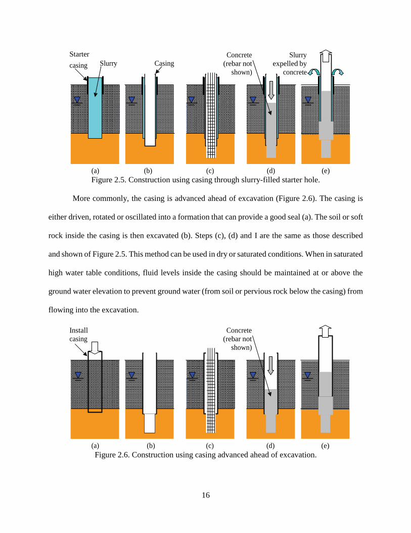
Figure 2.5. Construction using casing through slurry-filled starter hole 16

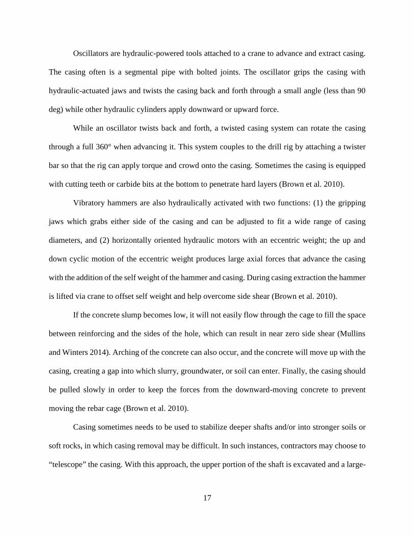
Figure 2.6. Construction using casing advanced ahead of excavation 16

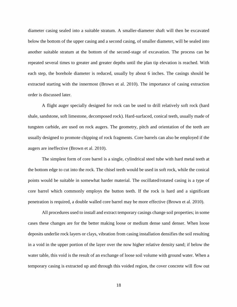
Figure 2.7. Conceptual process during casing extraction 19

Figure 2.8. Example case where concrete / water exchange was detected by fieldintegrity test 20

Figure 2.9. Concrete level differential (inside vs outside cage) with respect to cagetightness 21

Figure 2.10. Representation of the friction model for side shear in granular soils 26

Figure 2.11. Measured normalized lateral stress changes during shaft construction 32

Figure 2.12. Ultimate side resistance vs viscosity and slurry type 33

Figure 2.13. Variation of unit side shear with exposure time 34

Figure 2.14. Time effect on side shear from Opelika test shafts 36

Figure 2.15. Effects of exposure time, Canary Wharf site 38

Figure 2.16. Load vs displacement curves, Stratford site 39

Figure 2.17. Estimated side shear resistance 40

vi

Figure 2.18. Side shear vs exposure time 42

Figure 2.19. Load-displacement at top for test shafts in Jacksonville 44

Figure 3.1. Plan view layout of all 36 test shafts 50

Figure 3.2. Overview of the testing site 51

Figure 3.3. Simplified geotechnical profile and illustration of the shafts positioning 51

Figure 3.4. Phase 2 mixing and testing setup 53

Figure 3.5. Bentonite slurry mixing 53

Figure 3.6. Cetco polymer mixing 54

Figure 3.7. KBI polymer mixing 55

Figure 3.8. Matrix polymer mixing 55

Figure 3.9. Phase 3 shafts slurry mixing 56

Figure 3.10. Setup for the viscosity vs fluid loss study 56

Figure 3.11. Viscosity measurement during the construction of phase 2 shafts 57

Figure 3.12. Phase 2 shafts excavation (left) and predominant silty-sand soil (right) 59

Figure 3.13. Illustration of concrete placement 60

Figure 3.14. Concrete mixing for phase 2 shafts 61

Figure 3.15. Small-scale pull-out load tests setup 62

Figure 3.16. Overall view of the phase 2 testing area 62

Figure 3.17. Field pull-out load vs displacement for the 32 small-scale shafts 64

Figure 3.18. Maximum pull-out load vs exposure time 65

Figure 3.19. Side shear resistance vs exposure time 65

Figure 3.20. Variation of shafts stiffness over time 66

Figure 3.21. Variation of normalized stiffness over time 66

vii

Figure 3.22. Normalized side shear over time 67

Figure 3.23. Monitoring of fluid level on phase 2 shafts 68

Figure 3.24. Volumetric measurement of the slurry being introduced in the shafts (phase 2) 69

Figure 3.25. Illustration of the testing being performed overnight 70

Figure 3.26. Labeled buckets used on phase 3 shafts 70

Figure 3.27. Viscosity variation over time 71

Figure 3.28. Cumulative volume of slurry introduced on the shafts over time 72

Figure 3.29. Flow rate vs exposure time, phase 2 shafts 73

Figure 3.30. Cumulative slurry volume over time for different viscosities 74

Figure 3.31. Flow rate over time for different viscosities 74

Figure 4.1. Field retrieved limestone cores (left); core from simulated limestonebed and simulated limestone cylinder specimen (right) 76

Figure 4.2. Casting of simulated limestone bed 77

Figure 4.3. Debonding plastic disks (left) and centering rods (right) 77

Figure 4.4. Preparation of cylinders from limestone bed material 78

Figure 4.5. Rock socket construction layout on each simulated limestone bed 79

Figure 4.6. Casing cutting tips, drive shoe, casing extensions and drill rod couplers 80

Figure 4.7. Fine-tooth (left), coarse-tooth (center) and driving shoe (right) 80

Figure 4.8. Top of simulated limestone beds flooded with water and being pre-cored 81

Figure 4.9. Pre-drilling (left) and driving the casing (right) 82

Figure 4.10. Airlift vacuum used to clean up fragments from inside the installed casings 83

Figure 4.11. Rotatory casing installation (left) and drill bit (right) 84

Figure 4.12. Cuttings replacement on the outer perimeter of the casings 85

Figure 4.13. Example of high-resolution pictures taken on the control holes 85

viii

Figure 4.14. Concrete casting on the rock sockets 87

Figure 4.15. PVC tube containing the all-thread rod being pushed into the fresh concrete 87

Figure 4.16. Debonding plastic sleeves on top 8in of the sockets 88

Figure 4.17. Sockets immediately after concreting (left), ready for load testing(center and right) 88

Figure 4.18. Pull-out load test in progress 89

Figure 4.19. Extracted sockets from bed 5 (left), bed 1 (center) and bed 4 (right) 90

Figure 4.20. Load vs displacement for all sockets 92

Figure 4.21. Side shear resistance vs displacement for all sockets 95

Figure 4.22. Normalized side shear resistance (by bed UCS) vs displacement 96

Figure 4.23. Temporary / control side shear ratio vs displacement 98

Figure 5.1. Partial view of freshly concreted test shafts 100

Figure 5.2. Measured vs design side shear (O’Neill and Reese 1999) 101

Figure 5.3. Resistance bias factor based on O’Neill and Reese (1999) 102

Figure 5.4. Measured vs design side shear (Brown et al. 2010) 102

Figure 5.5. Resistance bias factor based on Brown et al. (2010) 103

Figure 5.6. Rock socketed specimens being prepared for pull-out tests 104

Figure 5.7. Design and measured side shear / UCS ratio vs simulated limestonebeds UCS 105

Figure 5.8. Resistance bias factor based on four methods – temporary casing sockets 106

Figure 5.9. Resistance factor vs reliability index – slurry effects research (0h – 96h) 112

Figure 5.10. Resistance factor vs reliability index – temporary casing effects research 113

Figure 5.11. Adjusted resistance factors – slurry study 115

Figure 5.12. Adjusted resistance factors – temporary casing study 116

ix

Figure A.1. CPT test results – shaft B48 126

Figure A.2. CPT test results – shaft B96 127

Figure A.3. CPT test results – shaft C48 128

Figure A.4. CPT test results – shaft C96 129

Figure A.5. CPT test results – shaft K48 130

Figure A.6. CPT test results – shaft K96 131

Figure A.7. CPT test results – shaft M48 132

Figure A.8. CPT test results – shaft M96 133

x

ABSTRACT

Design methods for side shear of drilled shafts, including the resistance factors that should

be applied, do not account for any specific construction procedure. Instead, design often relies on

analysis of case studies which include all construction methods used in each geomaterial type (e.g.

clays, sands and rocks), or on parametric analysis. Nonetheless, literature suggests that different

construction procedures result in varying side shear.

This research investigated 2 types of construction: (1) slurry stabilization in sandy soils

using bentonite and polymer products that are commonly used on the field, with exposure times

from near 0h to 96h, and (2) temporary casing stabilization in simulated limestone using 3 different

methods for installation and extraction of the casings which included: driven, coarse-tooth rotated

and fine-tooth rotated. All specimens were 1/10th scale in relation to the most common shafts sizes

constructed in the field.

The results showed that bentonite slurry causes a significant reduction on the side shear

within relatively short periods of time (between 2h and 4h of open excavation), whereas polymer

slurry did not show appreciable variations up to 96h.

The driven and coarse-tooth rotated temporary casing exhibited lower side shear resistance

than the fine-tooth rotated casings, which can be attributed to the larger annulus outside the casing

and the additional crumbled pieces of rock that degrades the contact interface with the socket

concrete.

Construction-based resistance factors are suggested for each construction procedure

investigated in this study and clearly show the effects from different methods.

1

CHAPTER 1: INTRODUCTION

Foundations are below ground structural elements responsible for distributing loads that

come from above ground structures. The loads can be due to the structure self-weight, occupants,

wind, rain / snow, earthquakes, vessel or vehicle impacts, machinery induced vibration and other

sources. Foundation elements can be shallow (footings), which have a large area of contact with

the soil but are relatively close to the ground surface, or deep, with high length to cross sectional

area ratios.

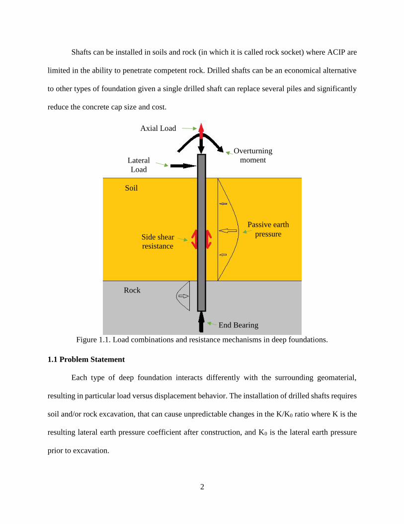
Deep foundation elements resist axial loads by side shear, end bearing or a combination

thereof; lateral and overturning loads depend on the ability of the adjacent geomaterial to provide

sufficient passive soil resistance (Figure 1.1). The two most common deep foundation types are

driven (piles) and cast-in place elements. Driven piles are commonly made of wood, steel, or

concrete; cast in place elements are made from concrete (or grout).

Cast-in-place elements are broken into two categories: augered-cast-in-place (ACIP) piles

and drilled shafts. ACIP piles differ from shafts in that a full depth continuous flight auger is used

to pierce the ground and as the auger is extracted, grout is pumped to replace the cylindrical volume

of the auger. Reinforcing steel is then placed in the fluid grout. Drilled shafts, (also known as

shafts, bored piles, drilled caissons, drilled piers and cast-in-drilled-hole piles) are cylindrical,

large diameter column-like reinforced concrete members. Shafts are typically between 2.5ft and

12ft in diameter (up to 30ft) and can have lengths that exceed 300ft. Shafts differ from ACIP piles

in that an open excavation is formed by the successive removal of soil or rock in relatively short

length increments (e.g. 1-2ft).

2

Shafts can be installed in soils and rock (in which it is called rock socket) where ACIP are

limited in the ability to penetrate competent rock. Drilled shafts can be an economical alternative

to other types of foundation given a single drilled shaft can replace several piles and significantly

reduce the concrete cap size and cost.

Figure 1.1. Load combinations and resistance mechanisms in deep foundations.

1.1 Problem Statement

Each type of deep foundation interacts differently with the surrounding geomaterial,

resulting in particular load versus displacement behavior. The installation of drilled shafts requires

soil and/or rock excavation, that can cause unpredictable changes in the K/K0 ratio where K is the

resulting lateral earth pressure coefficient after construction, and K0 is the lateral earth pressure

prior to excavation.

OverturningmomentLateral

Load

Axial Load

Side shearresistance

Passive earthpressure

End Bearing

Soil

Rock

3

The excavation for drilled shaft construction requires stabilization methods to prevent

collapse of the sidewalls. Typically, the stability of a drilled shaft excavation can be maintained

hydrostatically (drilling slurry), mechanically (permanent or temporary casing), or by a

combination of both. Each particular type of stabilization (drilling slurry, or temporary casing for

instance), can affect the resulting behavior of the shafts. These effects are not currently addressed

in present design methods. Upon closer review of current design methods, it becomes evident that

further refinements for side shear of drilled shafts could be implemented that address the different

types of excavation stabilization. The major objectives of this research program were:

Identify the effect of slurry type on side shear (e.g. mineral or polymer).

Identify if there is a time limit after which effects from drilling slurry (mineral and

polymer) exposure may exist, and quantify how the unit side shear changes due to the

effects from prolonged open excavation times.

Identify the magnitude of side shear variations that accompany the crumbling / degradation

of limestone around the temporary casing due to different casing types and installation /

extraction methods.

1.2 Organization of this Dissertation

This dissertation is divided into four ensuing chapters. Chapter two presents a literature

review of available publications regarding design methods and case studies pertaining to side shear

of drilled shafts in soils and rocks, primarily in sand and limestone. This chapter includes the

history of the development of the design methods as well as several case studies pertaining to

drilled shafts excavated under drilling slurry stabilization in sandy soils and the use of temporary

casings in limestone.

4

Chapters 3 and 4 present the research approach and results for both the influence of time

exposure to bentonite and polymer slurries on the side shear of drilled shafts over time, and the

effects of different types / methods of casing installation / extraction procedures on the side shear

of rock sockets in limestone, respectively. Chapter 3 also includes results of slurry fluid loss

experiments performed with polymer slurry at various viscosities.

Chapter 5 presents more in-depth analyses of the results presented in Chapters 3 and 4.

Discussions regarding the different observed side shear behavior due to each construction

procedure are included. The findings are extended to Load and Resistance Factor Design (LRFD)

concepts where the measured capacity is compared to predicted design capacity (bias). LRFD

resistance factors are suggested for each construction procedure that stem from the test program

results.

5

CHAPTER 2: REVIEW OF SIDE SHEAR BEHAVIOR OF DRILLED SHAFTS

Design methods used today to determine the side shear resistance of drilled shafts in soil

and rock were developed, mostly, using case studies and parametric evaluations to develop design

equations. However, despite the close link to actual field conditions (e.g. O’Neill and Reese 1999)

present design methods do not account for the unique features associated with each construction

procedure. Instead, a lower bound envelope that encompasses the majority of the observed

performance through analysis of load tests was proposed (both soils and rocks). On the other hand,

the FHWA 2010 Drilled Shaft Construction Manual proposed that a more theoretical approach,

based on geotechnical investigation results, is more suitable for defining the design side shear of

drilled shafts in sandy soils (Brown et al. 2010).

Both the FHWA (2010) and (AASHTO 2014) design manuals present similar equations

for computing the anticipated side shear of rock sockets. FDOT (2017a) requires the use of a

different method developed by McVay et al. (1992), which is also based on load test results, but

with relationships specifically to Florida limestone. Although the McVay method was supported

by results of laboratory unconfined compression and split tensile strengths on limestone specimens

taken from 14 load test sites in the field, it is theoretically linked to the Mohr-Coulomb failure

criteria. Again, methods to determine rock socket resistance while based on empirical field load

test results, still do not take into account the wide range of construction techniques (i.e. temporary

casing versus no casing) that can lead to varied side wall roughness and/or states of cleanliness.

6

According to O’Neill (1981), the factors that mostly influence the behavior of drilled shafts

include in-situ soil conditions, type and direction of loading, shaft geometry and, “very

importantly,” construction procedure. This chapter presents an overview of some of the most

commonly used design methods for side shear of drilled shafts in sandy soils and rocks, including

limitations. Case studies available in literature are included to illustrate, where possible, the

differences in side shear behavior from varied construction methods.

This dissertation focuses on how construction and excavation stabilization methods affect

the side shear resistance of a drilled shaft. The effects of concrete flow properties are not addressed.

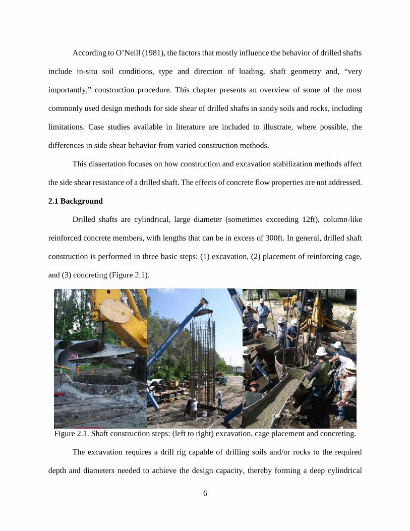
2.1 Background

Drilled shafts are cylindrical, large diameter (sometimes exceeding 12ft), column-like

reinforced concrete members, with lengths that can be in excess of 300ft. In general, drilled shaft

construction is performed in three basic steps: (1) excavation, (2) placement of reinforcing cage,

and (3) concreting (Figure 2.1).

Figure 2.1. Shaft construction steps: (left to right) excavation, cage placement and concreting.

The excavation requires a drill rig capable of drilling soils and/or rocks to the required

depth and diameters needed to achieve the design capacity, thereby forming a deep cylindrical

7

void space. Drill rigs are typically mechanically or hydraulically driven with telescopic Kelley

bars that are adjustable in length and attached to a single or multi-flight auger (Mullins and Winters

2014). Manuals that include construction procedures of drilled shafts, such as such as the FHWA

Drilled Shaft Construction Manual (O’Neill and Reese 1999; Brown et al. 2010) and state

specifications, present details for each type of construction procedure and its particularities.

On drilled shaft construction, the auger is not continuous-flight, but rather 2 or 3 flights.

Once the proper tip elevation is reached, the auger is replaced with a clean out bucket in order to

remove any loose material from the bottom of the excavation. The reinforcing cage is placed within

the excavation, followed by concrete. This process requires the in-situ soils/rocks to act as the

formwork and define the shape of the concrete (Mullins and Winters 2014).

2.2 Excavation Stabilization Techniques

Excavation stability and concreting are the two most important and yet difficult steps in

shaft construction. The side walls are held in place either by fluid slurry pressure inside the

excavation pressing outward on the excavated walls or by mechanical means afforded by the

strength of a casing (large diameter steel pipe). In the early 1900’s shaft excavations were

stabilized with vertical boards and lateral bracing; excavation was carried out via men in the hole,

but this method was only plausible in dry conditions.

2.2.1 Slurry Stabilization of Drilled Shafts

In cases where the ground water table is encountered within the design shaft depths, some

form of fluid must be maintained within the excavation to prevent intrusion of ground water. Use

of slurry stabilization is most commonly performed using mineral products (i.e. bentonite or

attapulgite) or synthetic polymeric compounds mixed with water. Using water alone is not a

common practice when there are no full length casings due to the enormous refill rates that would

8

be necessary to prevent borehole collapse (Mullins and Winters 2014). Support is provided by the

radially applied hydrostatic slurry pressure to the excavated walls, which requires the slurry level

to be maintained above the ground water table throughout the entire construction. The slurry inside

the excavation is typically mantained between 4 and 8 feet above the water table, depending on

the type of slurry (Mullins and Winters 2014).

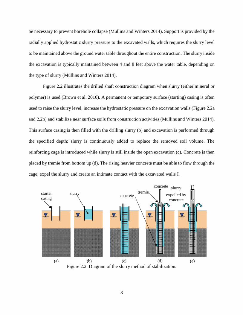
Figure 2.2 illustrates the drilled shaft construction diagram when slurry (either mineral or

polymer) is used (Brown et al. 2010). A permanent or temporary surface (starting) casing is often

used to raise the slurry level, increase the hydrostatic pressure on the excavation walls (Figure 2.2a

and 2.2b) and stabilize near surface soils from construction activities (Mullins and Winters 2014).

This surface casing is then filled with the drilling slurry (b) and excavation is performed through

the specified depth; slurry is continuously added to replace the removed soil volume. The

reinforcing cage is introduced while slurry is still inside the open excavation (c). Concrete is then

placed by tremie from bottom up (d). The rising heavier concrete must be able to flow through the

cage, expel the slurry and create an intimate contact with the excavated walls I.

concrete slurrystartercasing

slurry concretetremie

expelled byconcrete

(a) (b) (c) (d) (e)Figure 2.2. Diagram of the slurry method of stabilization.

9

Although both mineral and polymer slurry have been shown to be effective in stabilizing

an excavation (and now both permitted in most cases), the mechanisms by which they provide this

stability are quite different. Mineral slurries depend on minimum clay mineral concentration (0.3-

1.0lb/gal) to quickly seal the excavation walls. The layer of clay minerals that form on the walls is

called a filter cake (where the clay particles are filtered out of the slurry by the surrounding

permeable soils). When mineral slurry is mixed correctly, very little flow into the surrounding soil

occurs and the excess head differential between the slurry elevation and the ground water table is

directly converted to a lateral force.

Polymer slurry is more viscous than water which allows it to bind sandy soil in a quasi-

cohesive manner making it less susceptible to low pressure sloughing behind the auger. The

concentration of polymer products in the slurry are approximately 1/100th that of mineral slurry

and no filter cake forms. While polymer slurry will continue to flow, the flow rate will slow but

will not completely seal off the excavation walls (Mullins and Winters 2014). Nonetheless, similar

to mineral slurry, this outward flow also causes radially outward pressure on the walls, but to a

lesser level. As the density and lateral flow / pressure are lower for a given head differential,

polymer slurry levels must be maintained at higher levels than mineral slurry.

Depending on the soil type and slurry level maintenance, the excavation process may also

be accompanied by stress relaxation in the surrounding soil (Clayton and Milititsky 1983; O’Neill

2001). Filling the borehole with fluid concrete can partially or completely restore the in situ lateral

soil stresses (Bernal and Reese 1983; Chang and Zhu 2004). The available side shear resistance

depends on how much effective stress in the soil near the borehole is lost before the borehole is

concreted, how effective the concreting process is at restoring lateral stress in the soil, the degree

10

of roughness in the borehole, and the pore pressure response of the resulting modified soil (O’Neill

2001).

Bentonite is the common name for a type of mineral slurry, which is a processed powdered

clay consisting predominately of the mineral sodium montmorillonite. Other processed, powdered

clay minerals, such as attapulgite (calcium montmorillonite) and sepiolite, may also be used,

typically in saline groundwater conditions (Brown et al. 2010).

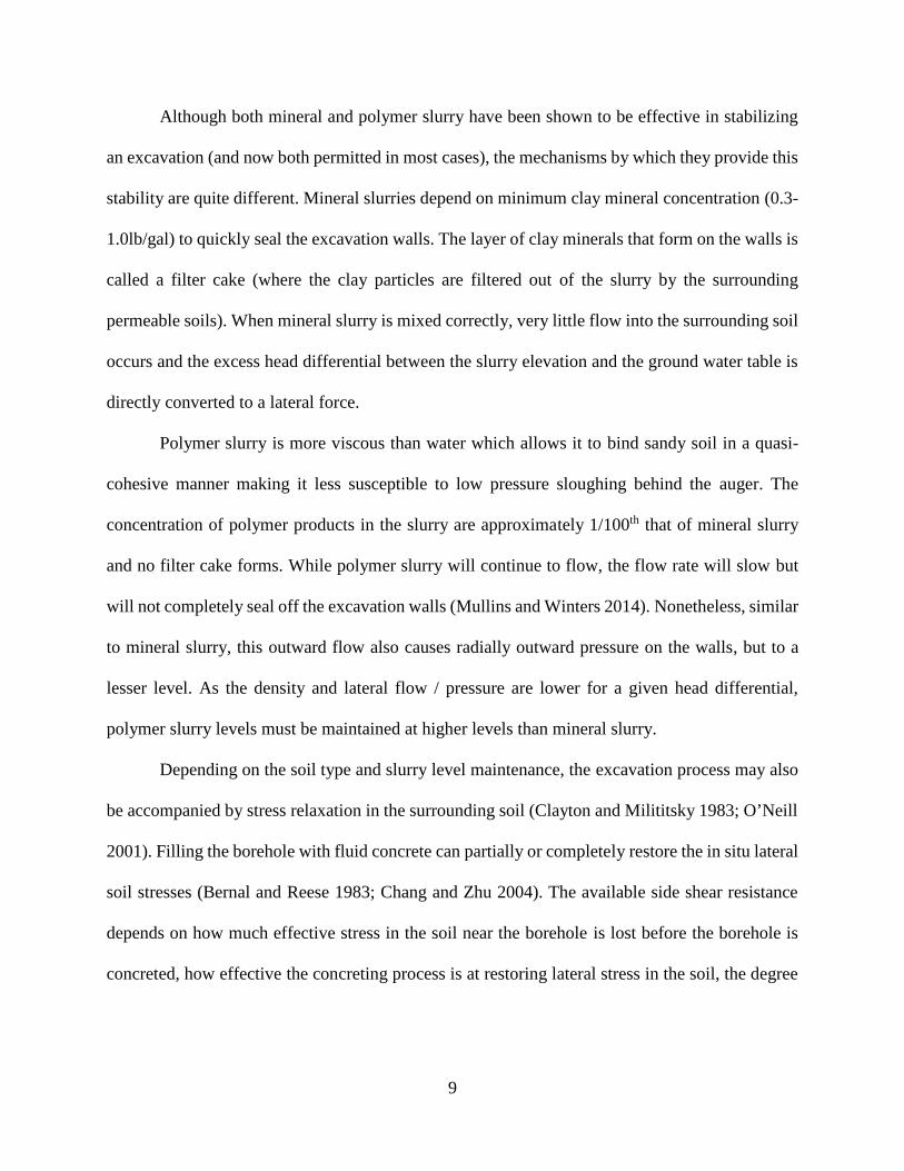
When introduced into a drilled shaft excavation, the mineral slurry contributes to borehole

stability through two mechanisms: formation of a filter cake, which effectively acts as a membrane

on the sidewalls of the borehole, and a positive fluid pressure acting against the filter cake

membrane and borehole sidewalls from increased density (Figure 2.3, Brown et al. 2010).

The filter cake is formed due to the hydration of the clay minerals (attapulgite,

montmorillonite and other expansive minerals), which creates the double layer, generating plate-

like particles that accumulate on the pores of permeable materials. The infiltration of this material

exhibits an aptness to form larger and larger nets that builds a seal in the geomaterial voids,

significantly decreasing the permeability. This phenomenon was observed by Terzaghi (1925),

Macey (1942) and Grace (1953), as summarized in Mesri and Olson (1971). The filter cake may

affect the effective shaft dimensions, especially in small diameter shafts, as observed by Majano

(1992).

The bentonite slurry will have a density a little greater than water alone from the suspended

slurry products; mineral slurry also develops gel strength which aids in the transport of cuttings

during excavation and concrete placement. During recirculation, the solids that are suspended on

the slurry increase the slurry density and can make it thicker (more viscous). If the slurry becomes

11

too heavy or viscous the integrity of the shaft can be at risk as it becomes more difficult to be

displaced by the fluid concrete.

Figure 2.3. Formation of filter cake and positive net pressure in granular soils.

The term polymer refers to any natural and synthetic compounds, usually of high molecular

weight, consisting of individual units (monomers) linked in a long, chain-like hydrocarbon

molecules. Synthetic polymer slurries made from acrylamide and acrylic acid, specifically termed

anionic polyacrylamide or PAM, entered the drilled shaft market in the 1980s. More recently,

advanced polymers made by combining polyacrylamides with other chemicals have been

introduced in an effort to improve performance while minimizing the need for additives.

Commercial polymer products vary in physical form (dry powder, granules, or liquids) and in the

details of the chemistry of the hydrocarbon molecules (molecular weight, molecule length, surface

charge density, etc., Brown et al. 2010).

Synthetic polymers can be made by modifying natural polymers. For example, carboxy-

methylcellulose (CMC) is made by reacting cellulose with chloracetic acid and NaOH, substituting

CH2COO-Na+ for H. In the cellulose unit, there are three OH groups, and each one is capable of

substitution. In general, the average number of carboxy groups (OH-C-H) on the chain per unit

12

cell is known as the “degree of substitution”. The carboxy group has the function of imparting

water solubility (or dispersability) to the polymer. It is also responsible for stretching linearly the

chains of polymer by creating negative charges that repel every unit from each other, therefore

increasing the viscosity of the polymer-based slurry.

Another common type of water soluble polymer is made of a polyacrylamide base. This

type of polymer is also an anionic polyelectrolyte which is made by converting some amides on a

polyacrylamide chain to carboxylates through hydrolysis (Majano 1992).

When polymer slurry is introduced, there is an initial fluid loss into the formation. This

penetration of polymer slurry into a porous formation allows the polymer to interact with the soil

particles by chemical adhesion, creating a bonding effect and improving stability. The strength of

adhesion varies significantly between polymer types and can be affected by various additives

(Brown et al. 2010).

Polymer slurries are designed to perform through continuous infiltration through

permeable formations (sand, silt, and permeable rock). The fluid loss is dependent on the viscosity,

time of excavation and slurry type. Care must be taken on rising the tool because it generates zones

of lower pressure behind the extracting tool, which can pull the soil walls in. There must be excess

pressure head to prevent this, even if the head is kept above the water table. The borehole stability

is produced by a combination of hydrostatic pressure and continuous percolation of the slurry

through the zone containing the polymer strands, in addition to the adhesion and three-dimensional

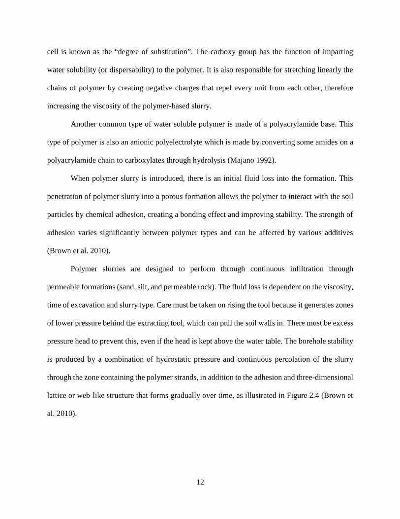
lattice or web-like structure that forms gradually over time, as illustrated in Figure 2.4 (Brown et

al. 2010).

13

Commercial polymer products vary in physical form (dry powder, granules, or liquids) and

in the details of the chemistry of the hydrocarbon molecules (molecular weight, molecule length,

surface charge density, etc.).

Figure 2.4. Borehole stabilization through polymer slurries.

The simpler PAM slurries may be sensitive to the presence of chloride (salt), free calcium,

magnesium and chlorine in the mixing water or groundwater (low pH). Unless the polymer has

been developed to remain stable in hard waters, typical upper limits for the concentration of

chloride, calcium and magnesium, and chlorine are 1500ppm, 100ppm and 50ppm, respectively

(Matrix 2016).

Usually, the quantification of the hardness of the water is done indirectly taking pH

measurements. If the pH is low, it has to be corrected to a range between 8 and 11, according to

design manuals. A commonly used product in the field is the soda ash. Some manufacturers have

developed its own products to correct the pH (Matrix 2016).

As mineral and polymer slurries are so different, different values for density, viscosity and

sand content (due to contamination during drilling) are imposed by state and federal specifications.

14

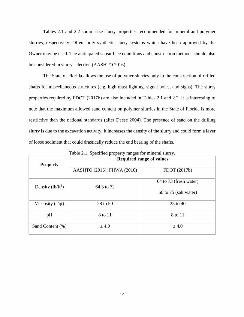
Tables 2.1 and 2.2 summarize slurry properties recommended for mineral and polymer

slurries, respectively. Often, only synthetic slurry systems which have been approved by the

Owner may be used. The anticipated subsurface conditions and construction methods should also

be considered in slurry selection (AASHTO 2016).

The State of Florida allows the use of polymer slurries only in the construction of drilled

shafts for miscellaneous structures (e.g. high mast lighting, signal poles, and signs). The slurry

properties required by FDOT (2017b) are also included in Tables 2.1 and 2.2. It is interesting to

note that the maximum allowed sand content on polymer slurries in the State of Florida is more

restrictive than the national standards (after Deese 2004). The presence of sand on the drilling

slurry is due to the excavation activity. It increases the density of the slurry and could form a layer

of loose sediment that could drastically reduce the end bearing of the shafts.

Table 2.1. Specified property ranges for mineral slurry.

PropertyRequired range of values

AASHTO (2016); FHWA (2010) FDOT (2017b)

Density (lb/ft3) 64.3 to 7264 to 73 (fresh water)

66 to 75 (salt water)

Viscosity (s/qt) 28 to 50 28 to 40

pH 8 to 11 8 to 11

Sand Content (%) ≤ 4.0 ≤ 4.0

15

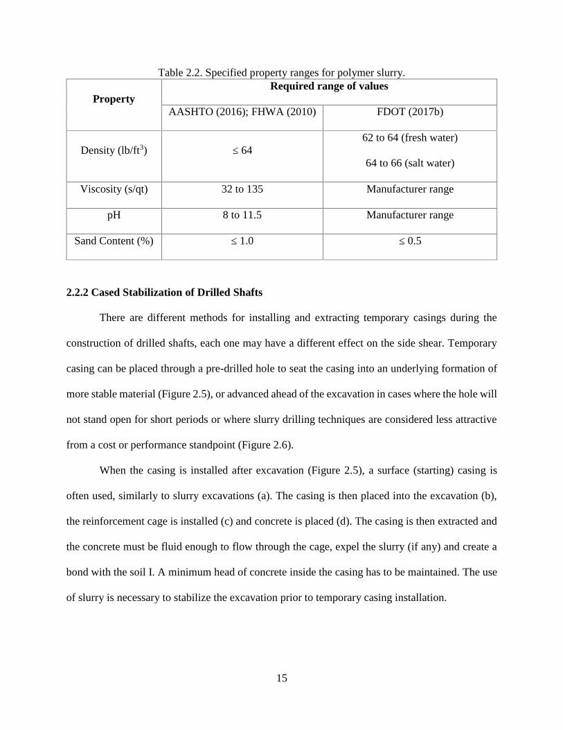
Table 2.2. Specified property ranges for polymer slurry.

PropertyRequired range of values

AASHTO (2016); FHWA (2010) FDOT (2017b)

Density (lb/ft3) ≤ 6462 to 64 (fresh water)

64 to 66 (salt water)

Viscosity (s/qt) 32 to 135 Manufacturer range

pH 8 to 11.5 Manufacturer range

Sand Content (%) ≤ 1.0 ≤ 0.5

2.2.2 Cased Stabilization of Drilled Shafts

There are different methods for installing and extracting temporary casings during the

construction of drilled shafts, each one may have a different effect on the side shear. Temporary

casing can be placed through a pre-drilled hole to seat the casing into an underlying formation of

more stable material (Figure 2.5), or advanced ahead of the excavation in cases where the hole will

not stand open for short periods or where slurry drilling techniques are considered less attractive

from a cost or performance standpoint (Figure 2.6).

When the casing is installed after excavation (Figure 2.5), a surface (starting) casing is

often used, similarly to slurry excavations (a). The casing is then placed into the excavation (b),

the reinforcement cage is installed (c) and concrete is placed (d). The casing is then extracted and

the concrete must be fluid enough to flow through the cage, expel the slurry (if any) and create a

bond with the soil I. A minimum head of concrete inside the casing has to be maintained. The use

of slurry is necessary to stabilize the excavation prior to temporary casing installation.

16

Starter

casing Slurry CasingConcrete

(rebar notshown)

Slurryexpelled by

concrete

(a) (b) (c) (d) (e)Figure 2.5. Construction using casing through slurry-filled starter hole.

More commonly, the casing is advanced ahead of excavation (Figure 2.6). The casing is

either driven, rotated or oscillated into a formation that can provide a good seal (a). The soil or soft

rock inside the casing is then excavated (b). Steps (c), (d) and I are the same as those described

and shown of Figure 2.5. This method can be used in dry or saturated conditions. When in saturated

high water table conditions, fluid levels inside the casing should be maintained at or above the

ground water elevation to prevent ground water (from soil or pervious rock below the casing) from

flowing into the excavation.

Installcasing

Concrete(rebar not

shown)

(a) (b) (c) (d) (e)Figure 2.6. Construction using casing advanced ahead of excavation.

17

Oscillators are hydraulic-powered tools attached to a crane to advance and extract casing.

The casing often is a segmental pipe with bolted joints. The oscillator grips the casing with

hydraulic-actuated jaws and twists the casing back and forth through a small angle (less than 90

deg) while other hydraulic cylinders apply downward or upward force.

While an oscillator twists back and forth, a twisted casing system can rotate the casing

through a full 360° when advancing it. This system couples to the drill rig by attaching a twister

bar so that the rig can apply torque and crowd onto the casing. Sometimes the casing is equipped

with cutting teeth or carbide bits at the bottom to penetrate hard layers (Brown et al. 2010).

Vibratory hammers are also hydraulically activated with two functions: (1) the gripping

jaws which grabs either side of the casing and can be adjusted to fit a wide range of casing

diameters, and (2) horizontally oriented hydraulic motors with an eccentric weight; the up and

down cyclic motion of the eccentric weight produces large axial forces that advance the casing

with the addition of the self weight of the hammer and casing. During casing extraction the hammer

is lifted via crane to offset self weight and help overcome side shear (Brown et al. 2010).

If the concrete slump becomes low, it will not easily flow through the cage to fill the space

between reinforcing and the sides of the hole, which can result in near zero side shear (Mullins

and Winters 2014). Arching of the concrete can also occur, and the concrete will move up with the

casing, creating a gap into which slurry, groundwater, or soil can enter. Finally, the casing should

be pulled slowly in order to keep the forces from the downward-moving concrete to prevent

moving the rebar cage (Brown et al. 2010).

Casing sometimes needs to be used to stabilize deeper shafts and/or into stronger soils or

soft rocks, in which casing removal may be difficult. In such instances, contractors may choose to

“telescope” the casing. With this approach, the upper portion of the shaft is excavated and a large-

18

diameter casing sealed into a suitable stratum. A smaller-diameter shaft will then be excavated

below the bottom of the upper casing and a second casing, of smaller diameter, will be sealed into

another suitable stratum at the bottom of the second-stage of excavation. The process can be

repeated several times to greater and greater depths until the plan tip elevation is reached. With

each step, the borehole diameter is reduced, usually by about 6 inches. The casings should be

extracted starting with the innermost (Brown et al. 2010). The importance of casing extraction

order is discussed later.

A flight auger specially designed for rock can be used to drill relatively soft rock (hard

shale, sandstone, soft limestone, decomposed rock). Hard-surfaced, conical teeth, usually made of

tungsten carbide, are used on rock augers. The geometry, pitch and orientation of the teeth are

usually designed to promote chipping of rock fragments. Core barrels can also be employed if the

augers are ineffective (Brown et al. 2010).

The simplest form of core barrel is a single, cylindrical steel tube with hard metal teeth at

the bottom edge to cut into the rock. The chisel teeth would be used in soft rock, while the conical

points would be suitable in somewhat harder material. The oscillated/rotated casing is a type of

core barrel which commonly employs the button teeth. If the rock is hard and a significant

penetration is required, a double walled core barrel may be more effective (Brown et al. 2010).

All procedures used to install and extract temporary casings change soil properties; in some

cases these changes are for the better making loose or medium dense sand denser. When loose

deposits underlie rock layers or clays, vibration from casing installation densifies the soil resulting

in a void in the upper portion of the layer over the now higher relative density sand; if below the

water table, this void is the result of an exchange of loose soil volume with ground water. When a

temporary casing is extracted up and through this voided region, the cover concrete will flow out

19

first to fill the void and some exchange of water and concrete occurs. This was described by

Sliwinski et al. (1984) and illustrated in Figure 2.7, where a water-filled void around the casing

(1) is filled by denser, higher pressure fluid concrete (2) resulting in trapped water inside casing

or shaft volume (3).

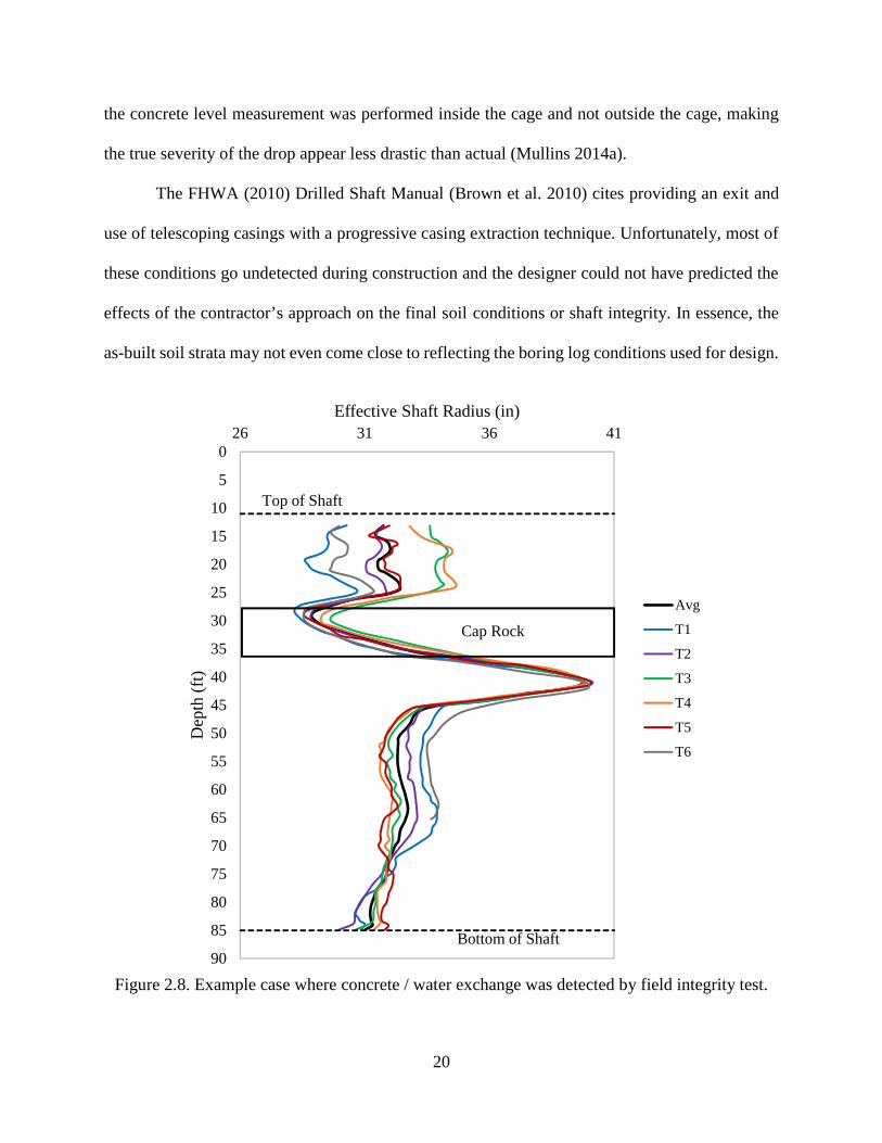
In a local case in south Florida (Mullins 2014a), the scenario described by Sliwinski was

observed where a significant drop in concrete level inside the temporary casing occurred during

casing extraction. Figure 2.8 shows the predicted shaft radius from thermal profiling which

indicated concrete within the permanent casing region (above 30ft depth) was less than that of the

casing. Below the cap rock, the shaft was oversized (design radius was 30in). This problem can be

a by-product of temporary casing (Mullins 2014a).

Figure 2.7. Conceptual process during casing extraction.

In the case shown by Figure 2.8 the concrete was sufficiently fluid to flow into the

surrounding void, and where no alternate exit for the incompressible water in the void was

available. It should also be noted that the core concrete level falls much slower due to the cage

obstruction making the cover region more prone to water intrusion/fluid exchange. Unfortunately,

(1) (2) (3)

Clay

Sand

Water

Concrete

20

the concrete level measurement was performed inside the cage and not outside the cage, making

the true severity of the drop appear less drastic than actual (Mullins 2014a).

The FHWA (2010) Drilled Shaft Manual (Brown et al. 2010) cites providing an exit and

use of telescoping casings with a progressive casing extraction technique. Unfortunately, most of

these conditions go undetected during construction and the designer could not have predicted the

effects of the contractor’s approach on the final soil conditions or shaft integrity. In essence, the

as-built soil strata may not even come close to reflecting the boring log conditions used for design.

Figure 2.8. Example case where concrete / water exchange was detected by field integrity test.

0

5

10

15

20

25

30

35

40

45

50

55

60

65

70

75

80

85

90

26 31 36 41

Dep

th (

ft)

Effective Shaft Radius (in)

Avg

T1

T2

T3

T4

T5

T6

Top of Shaft

Bottom of Shaft

Cap Rock

21

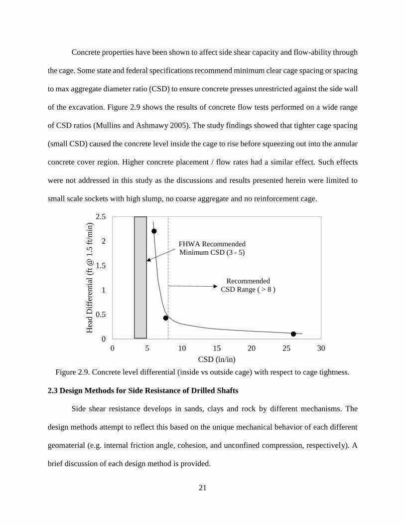
Concrete properties have been shown to affect side shear capacity and flow-ability through

the cage. Some state and federal specifications recommend minimum clear cage spacing or spacing

to max aggregate diameter ratio (CSD) to ensure concrete presses unrestricted against the side wall

of the excavation. Figure 2.9 shows the results of concrete flow tests performed on a wide range

of CSD ratios (Mullins and Ashmawy 2005). The study findings showed that tighter cage spacing

(small CSD) caused the concrete level inside the cage to rise before squeezing out into the annular

concrete cover region. Higher concrete placement / flow rates had a similar effect. Such effects

were not addressed in this study as the discussions and results presented herein were limited to

small scale sockets with high slump, no coarse aggregate and no reinforcement cage.

Figure 2.9. Concrete level differential (inside vs outside cage) with respect to cage tightness.

2.3 Design Methods for Side Resistance of Drilled Shafts

Side shear resistance develops in sands, clays and rock by different mechanisms. The

design methods attempt to reflect this based on the unique mechanical behavior of each different

geomaterial (e.g. internal friction angle, cohesion, and unconfined compression, respectively). A

brief discussion of each design method is provided.

0

0.5

1

1.5

2

2.5

0 5 10 15 20 25 30

Hea

d D

iffe

rent

ial (

ft @

1.5

ft/

min

)

CSD (in/in)

FHWA RecommendedMinimum CSD (3 - 5)

RecommendedCSD Range ( > 8 )

22

2.3.1 Design Methods for Sandy Soils

Side shear resistance is the dominant load carrying component in shafts; end bearing can

be considered, but only to a far lesser degree. This study again focuses on side shear and how it is

affected by construction methods.

Several methods to estimate the ultimate side shear resistance for shafts in sand have been

developed. Two of them are discussed in this dissertation: (1) Reese and Oneill (1988a) and

O’Neill and Hassan (1994), which were last updated in the 1999 version of the FHWA Drilled

Shafts Manual (O’Neil and Reese 1999), and (2) Brown et al. (2010), based on the work of Chen

and Kulhawy (2002), which was recommended by the 2010 version of the FHWA Drilled Shafts

Manual and by AASHTO after 2014.

Essentially, in sandy soils cohesion I is zero and the side shear resistance (fsmax) becomes

a function of the effective internal friction angle (’) and the effective vertical overburden stress

(σ’v). Based on this, Touma (1972), and Touma and Reese (1972) presented analyses of side shear

behavior of drilled shafts in sandy soils using the following equation, in which alpha () does not

relate to the alpha method; instead, it was the beginning of the beta methods:fs = α ∗ σ v ∗ tan( ) eqn. 2.1

O’Neill and Reese (1978) suggested that the side shear resistance of drilled shafts in sands

would be proportional to a parameter then called , and it would be a function of the ratio between

the final (after construction) lateral earth pressure coefficient and the corresponding at rest value,

and the ratio between the shaft to concrete and soil to soil friction angle. The parameter was

suggested as a representation of how construction would change these ratios. The side shear

resistance of drilled shafts was further defined as a relationship between and the effective vertical

overburden stress, σ’v (O’Neill and Reese 1978):

23

fsmax = ∗ σ v eqn. 2.2

The two methods discussed herein derive from this same approach, though one of them

recommended equations for based on analysis of case studies, and the other suggested that a

more theoretical approach would be more suitable.

The original beta method was last updated by O’Neill and Reese (1999) in the 1999 FHWA

Drilled Shaft Manual, which was also adopted by AASHTO until 2014. The resulting equations

for calculating beta were based on the work of Reese and O’Neill (1988a), with contributions of

O’Neill and Hassan (1994). The equations recommended for the coefficient were based on the

following equation:β = ∗ Ko ∗ tan ′

eqn. 2.3

In equation 2.3, K0 is the at rest lateral earth pressure, K is the resulting lateral earth

pressure after construction, ’ is the soil friction angle and is the friction angle between soil and

shaft concrete. Note that equation 2.3 can be simplified, but it highlights the ratios (K/K0) and

(/’), which have been investigated by several authors.

Both (K/K0) and (/’) are very difficult to evaluate for any particular drilled shaft because

they are highly dependent on the construction procedures. Whether the contractor is using a drilling

tool that is appropriate to the soil encountered or is excessively rotating the tool in the hole; the

length of time the borehole remains open; whether drilling slurry is used and when during the

drilling process the slurry is introduced into the borehole; the length of time drilling slurry

(especially mineral slurry) remains unagitated in the borehole; the diameter of the borehole; the

grain-size distribution of the soil (as it relates to arching of stresses in the soil), and many similar

factors which had not been individually quantified (O’Neill and Reese 1999).

24

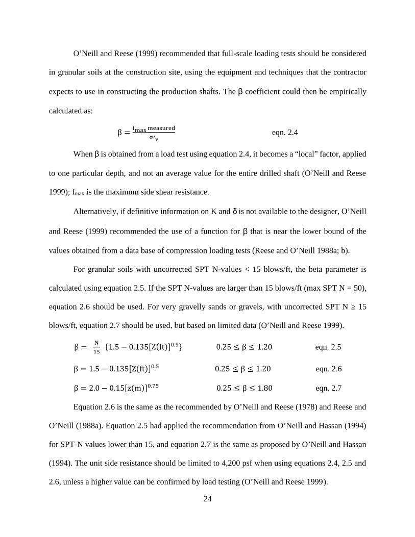
O’Neill and Reese (1999) recommended that full-scale loading tests should be considered

in granular soils at the construction site, using the equipment and techniques that the contractor

expects to use in constructing the production shafts. The coefficient could then be empirically

calculated as: β = eqn. 2.4

When is obtained from a load test using equation 2.4, it becomes a “local” factor, applied

to one particular depth, and not an average value for the entire drilled shaft (O’Neill and Reese

1999); fmax is the maximum side shear resistance.

Alternatively, if definitive information on K and is not available to the designer, O’Neill

and Reese (1999) recommended the use of a function for that is near the lower bound of the

values obtained from a data base of compression loading tests (Reese and O’Neill 1988a; b).

For granular soils with uncorrected SPT N-values < 15 blows/ft, the beta parameter is

calculated using equation 2.5. If the SPT N-values are larger than 15 blows/ft (max SPT N = 50),

equation 2.6 should be used. For very gravelly sands or gravels, with uncorrected SPT N ≥ 15

blows/ft, equation 2.7 should be used, but based on limited data (O’Neill and Reese 1999).β = {1.5 − 0.135[Z(ft)] . } 0.25 ≤ β ≤ 1.20 eqn. 2.5β = 1.5 − 0.135[Z(ft)] . 0.25 ≤ β ≤ 1.20 eqn. 2.6β = 2.0 − 0.15[z(m)] . 0.25 ≤ β ≤ 1.80 eqn. 2.7

Equation 2.6 is the same as the recommended by O’Neill and Reese (1978) and Reese and

O’Neill (1988a). Equation 2.5 had applied the recommendation from O’Neill and Hassan (1994)

for SPT-N values lower than 15, and equation 2.7 is the same as proposed by O’Neill and Hassan

(1994). The unit side resistance should be limited to 4,200 psf when using equations 2.4, 2.5 and

2.6, unless a higher value can be confirmed by load testing (O’Neill and Reese 1999).

25

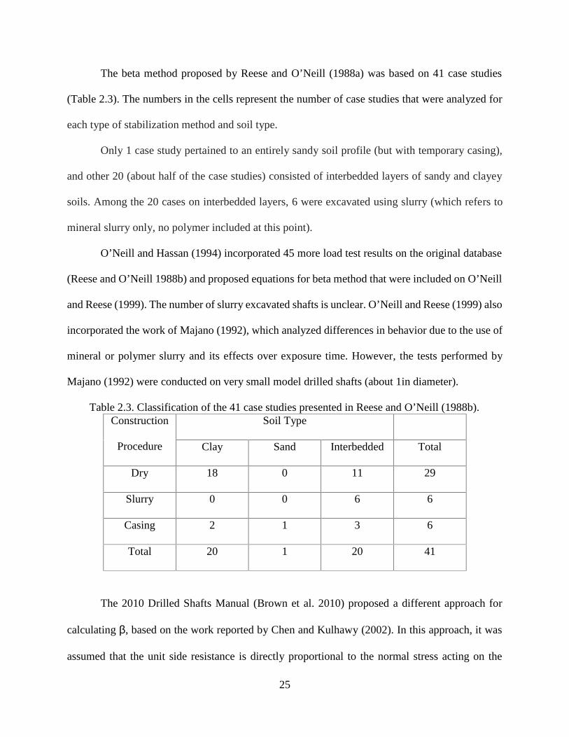
The beta method proposed by Reese and O’Neill (1988a) was based on 41 case studies

(Table 2.3). The numbers in the cells represent the number of case studies that were analyzed for

each type of stabilization method and soil type.

Only 1 case study pertained to an entirely sandy soil profile (but with temporary casing),

and other 20 (about half of the case studies) consisted of interbedded layers of sandy and clayey

soils. Among the 20 cases on interbedded layers, 6 were excavated using slurry (which refers to

mineral slurry only, no polymer included at this point).

O’Neill and Hassan (1994) incorporated 45 more load test results on the original database

(Reese and O’Neill 1988b) and proposed equations for beta method that were included on O’Neill

and Reese (1999). The number of slurry excavated shafts is unclear. O’Neill and Reese (1999) also

incorporated the work of Majano (1992), which analyzed differences in behavior due to the use of

mineral or polymer slurry and its effects over exposure time. However, the tests performed by

Majano (1992) were conducted on very small model drilled shafts (about 1in diameter).

Table 2.3. Classification of the 41 case studies presented in Reese and O’Neill (1988b).Construction

Procedure

Soil Type

Clay Sand Interbedded Total

Dry 18 0 11 29

Slurry 0 0 6 6

Casing 2 1 3 6

Total 20 1 20 41

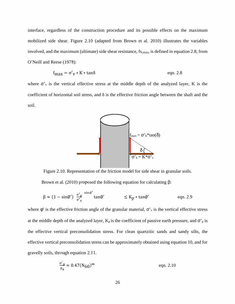
The 2010 Drilled Shafts Manual (Brown et al. 2010) proposed a different approach for

calculating , based on the work reported by Chen and Kulhawy (2002). In this approach, it was

assumed that the unit side resistance is directly proportional to the normal stress acting on the

26

interface, regardless of the construction procedure and its possible effects on the maximum

mobilized side shear. Figure 2.10 (adapted from Brown et al. 2010) illustrates the variables

involved, and the maximum (ultimate) side shear resistance, fs,max, is defined in equation 2.8, from

O’Neill and Reese (1978):fmax = σ v ∗ K ∗ tanδ eqn. 2.8

where ’v is the vertical effective stress at the middle depth of the analyzed layer, K is the

coefficient of horizontal soil stress, and δ is the effective friction angle between the shaft and the

soil.

Figure 2.10. Representation of the friction model for side shear in granular soils.

Brown et al. (2010) proposed the following equation for calculating :

β ≈ (1 − sin∅ ) ∅ tan∅ ≤ Kp ∗ tan∅ eqn. 2.9

where ’ is the effective friction angle of the granular material, ’v is the vertical effective stress

at the middle depth of the analyzed layer, Kp is the coefficient of passive earth pressure, and ’p is

the effective vertical preconsolidation stress. For clean quartzitic sands and sandy silts, the

effective vertical preconsolidation stress can be approximately obtained using equation 10, and for

gravelly soils, through equation 2.11.≈ 0.47(N60) eqn. 2.10

’h = K*’v

fmax = ’h*tan()

27

= 0.15N60 eqn. 2.11

where pa is the atmospheric pressure, and N60 is the corrected SPT N-value, corresponding to an

efficiency of 60%.

In the approach described above, it is assumed that no change in horizontal stress, and

therefore no change in K, should occur because of construction (Brown et al. 2010).

The beta method proposed by Kulhawy and Chen (2002) was based on 58 field load test

results (27 in uplift and 31 in compression). Among the 27 shafts tested in uplift, 5 were

constructed using slurry and 22, dry. Slurry was used on 7 of the compression shafts, 3 used casing

and 21 were constructed dry (Kulhawy and Chen 2002). It is unclear if polymer was used as a type

of drilling slurry.

The methods for design side shear of drilled shafts in sands ( methods) were, again,

developed considering all used construction procedures and did not account for particular effects

on the actual side shear, although differences were observed by O’Neill and Reese (1999) and

Kulhawy and Chen (2002). The shafts constructed using slurry were minority; most of the shafts

on the methods database were excavated dry.

2.3.2 Design Methods for Rock Socketed Shafts

The side shear strength of rock-socketed drilled shafts is similar to that of clayey soils in

that it is dependent on the in situ shear strength of the bearing strata. In this case, rock cores are

taken from the field and tested using various methods. Specifically, mean failure stresses from two

tests are commonly used: the unconfined compression test, qu, and the splitting tensile test, qt.

Local experience and results from load tests can provide the best insight into the most appropriate

approach (Mullins 2014b).

28

Side resistance in rock depends upon factors other than solely the strength of the

geomaterial. These include the roughness of the socket, the presence of soft seams within the

geomaterial, and the angle of friction between the concrete and geomaterial. The first

recommendation that O’Neill and Reese (1999) provided was to decide whether the socket will be

smooth or rough, since roughness of the borehole wall has a large effect on side resistance.

It was recommended that, unless the sides of the borehole are artificially roughened during

construction, the socket is considered smooth; however, procedures must guarantee that no

smeared material remains on the sides of the borehole. For design purposes, a smooth socket

contains a roughness naturally created with the drilling tool, but without leaving smeared material

on the sides of the borehole wall (Hassan and O’Neill 1997).

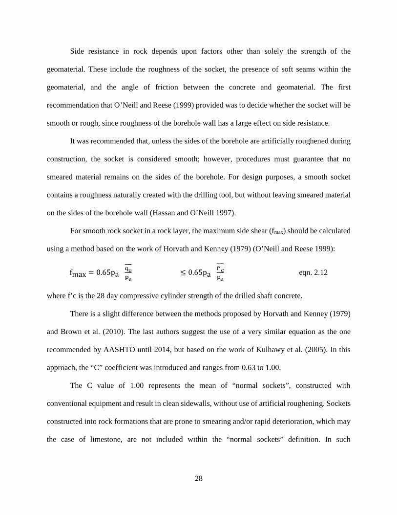
For smooth rock socket in a rock layer, the maximum side shear (fmax) should be calculated

using a method based on the work of Horvath and Kenney (1979) (O’Neill and Reese 1999):

fmax = 0.65pa ≤ 0.65pa eqn. 2.12

where f’c is the 28 day compressive cylinder strength of the drilled shaft concrete.

There is a slight difference between the methods proposed by Horvath and Kenney (1979)

and Brown et al. (2010). The last authors suggest the use of a very similar equation as the one

recommended by AASHTO until 2014, but based on the work of Kulhawy et al. (2005). In this

approach, the “C” coefficient was introduced and ranges from 0.63 to 1.00.

The C value of 1.00 represents the mean of “normal sockets”, constructed with

conventional equipment and result in clean sidewalls, without use of artificial roughening. Sockets

constructed into rock formations that are prone to smearing and/or rapid deterioration, which may

the case of limestone, are not included within the “normal sockets” definition. In such

29

circumstances, Brown et al. (2010) not explicitly suggests using a lower bound value for “C” of

0.63, which encompasses 90% of the load test results analyzed by Kulhawy et al. (2005).

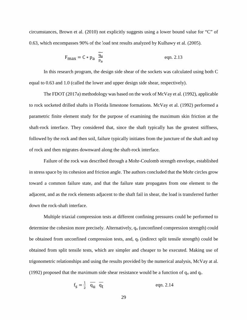
Fmax = C ∗ pa eqn. 2.13

In this research program, the design side shear of the sockets was calculated using both C

equal to 0.63 and 1.0 (called the lower and upper design side shear, respectively).

The FDOT (2017a) methodology was based on the work of McVay et al. (1992), applicable

to rock socketed drilled shafts in Florida limestone formations. McVay et al. (1992) performed a

parametric finite element study for the purpose of examining the maximum skin friction at the

shaft-rock interface. They considered that, since the shaft typically has the greatest stiffness,

followed by the rock and then soil, failure typically initiates from the juncture of the shaft and top

of rock and then migrates downward along the shaft-rock interface.

Failure of the rock was described through a Mohr-Coulomb strength envelope, established

in stress space by its cohesion and friction angle. The authors concluded that the Mohr circles grow

toward a common failure state, and that the failure state propagates from one element to the

adjacent, and as the rock elements adjacent to the shaft fail in shear, the load is transferred further

down the rock-shaft interface.

Multiple triaxial compression tests at different confining pressures could be performed to

determine the cohesion more precisely. Alternatively, qu (unconfined compression strength) could

be obtained from unconfined compression tests, and, qt (indirect split tensile strength) could be

obtained from split tensile tests, which are simpler and cheaper to be executed. Making use of

trigonometric relationships and using the results provided by the numerical analysis, McVay at al.

(1992) proposed that the maximum side shear resistance would be a function of qu and qt.fs = qu qt eqn. 2.14

30

Hudyma and Hiltunen (2014) argued that the large variability of the Florida limestone

properties should be incorporated into the design in order to obtain the design side shear

(ultimate/nominal) by applying the average recovery from the coring. FDOT (2017a) recommends

that the design side shear should be calculated as:fs = REC ∗ qu qt eqn. 2.15

where REC is the recovery expressed in decimals.

The method proposed by McVay et al. (1992) for rock sockets into Florida limestone and

adopted by FDOT (2017a) was supported by 14 case studies and over a thousand unconfined and

split tensile tests performed on recovered rock cores. The unconfined compressive strength (UCS)

from McVay at al. (1992) database ranged from 160psi to 1,400psi on the limestone samples tested,

and the split tensile strength, from 47psi to 166psi. The particular effects of using casings

(permanent or temporary) were not considered in the basis of this design method.

2.4 Case Studies

2.4.1 Case Studies with Slurry Stabilized Excavations

Numerous studies about the effects of slurry type on drilled shaft capacity have been

published, and yet there is no consensus agreement about the differences in side shear due to use

of bentonite or synthetic polymer slurry. Depending on the soil type, bentonite may leave no filter

cake (i.e. clayey soils) (Clayton and Milititsky 1983) due to little radial permeation into those soils.

Furthermore, the availability of publications that discuss the effects of longer exposure times to

bentonite and polymer slurry are scarce and, in general, limited to 36h.

Research by Reese et al. (1973) and Fleming and Sliwinski (1977) has showed that proper

use of slurry does not reduce the side resistance of drilled shafts, provided that the slurry and fluid

concrete are handled so that the slurry is displaced during concrete placement and concrete is

31

placed as soon as possible after the excavation is complete (Turner 1992). This could be virtually

true if actual 0h exposure times could occur either in practice or research. For longer exposure

times, soil relaxation may introduce changes on the K/K0 ratio.

In reality, most variations between test shafts are due to soil strength, concrete or

inadvertent construction variations. Studies reported by Mullins (2012) and Mullins and Winters

(2014) showed that using of polymer slurry did not adversely affect side shear capacity but rather

a modest improvement was noted. This finding was also reported by Majano (1992). Intuitively

many feel that the slick / slippery texture of polymer slurry materials may lubricate the soil particle

interfaces, but the high pH of the concrete is hypothesized to break down the polymer and eliminate

this effect. However, the concrete does not penetrate the soil as deeply as the slurry and would not

prevent “lubrication” of the more peripheral soils.

Chang and Zhu (2004) monitored the changes in horizontal stress in the ground during the

construction of a 2.6ft diameter and 98ft long drilled shaft, adjacent to the excavation, at a piling

site at Singapore. The upper part of the ground consisted of over 26ft of compacted residual soil

fill, classified as predominantly sandy silt, containing a fraction of clay. The ground water table

was encountered at 62ft depth.

One flat dilatometer was installed and left in place 1.6ft away from the borehole wall, at

the depth of 14.7ft (within the compacted fill) 5 days prior to pile construction. The initial

membrane lift off pressure (p0i) was measured before the excavation, and subsequent membrane

lift off pressure (p0) measurements were performed to monitor the changes in horizontal stress

throughout the construction (Figure 2.11). After some localized collapses (indicating loss of

stability), the piling contractor decided to fill up the excavation with water. Casting of concrete

32

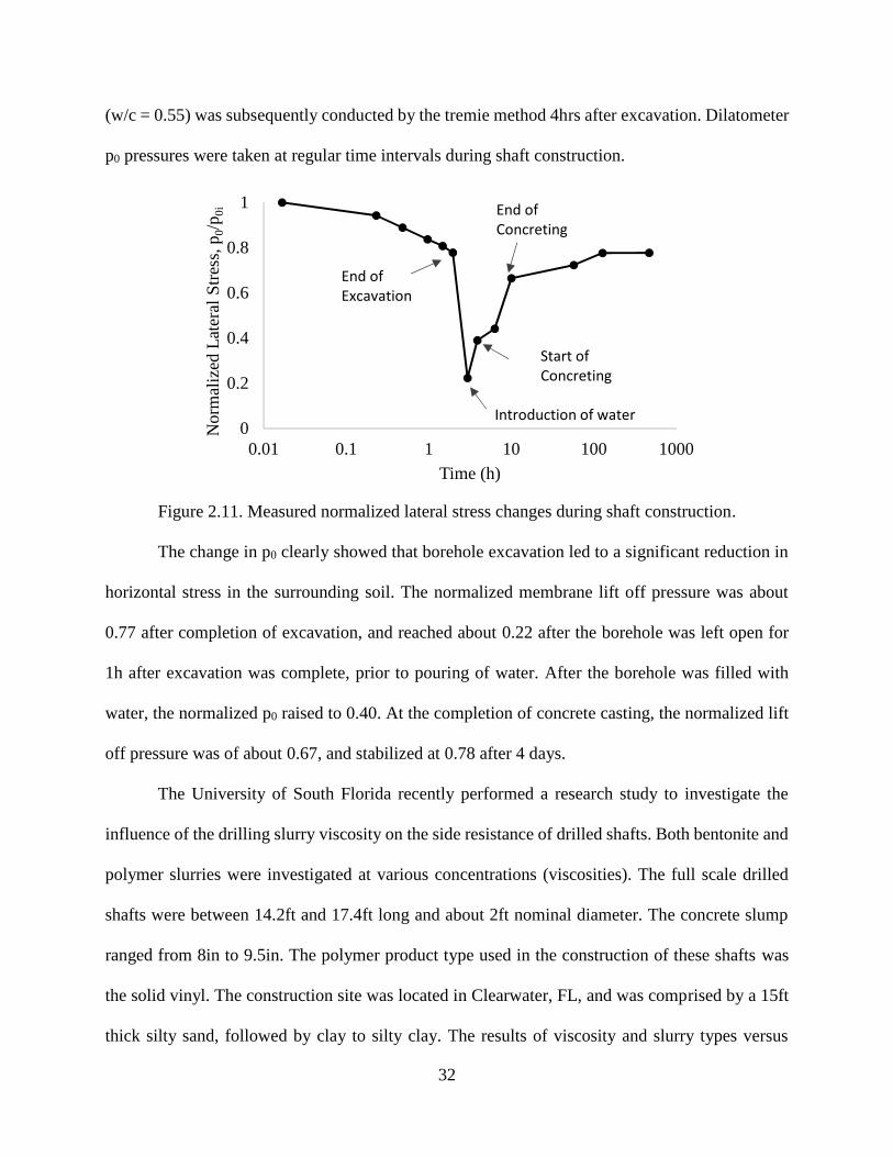
(w/c = 0.55) was subsequently conducted by the tremie method 4hrs after excavation. Dilatometer

p0 pressures were taken at regular time intervals during shaft construction.

Figure 2.11. Measured normalized lateral stress changes during shaft construction.

The change in p0 clearly showed that borehole excavation led to a significant reduction in

horizontal stress in the surrounding soil. The normalized membrane lift off pressure was about

0.77 after completion of excavation, and reached about 0.22 after the borehole was left open for

1h after excavation was complete, prior to pouring of water. After the borehole was filled with

water, the normalized p0 raised to 0.40. At the completion of concrete casting, the normalized lift

off pressure was of about 0.67, and stabilized at 0.78 after 4 days.

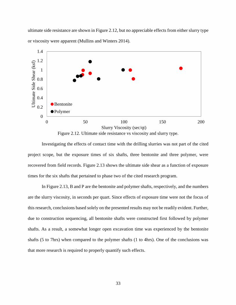
The University of South Florida recently performed a research study to investigate the

influence of the drilling slurry viscosity on the side resistance of drilled shafts. Both bentonite and

polymer slurries were investigated at various concentrations (viscosities). The full scale drilled

shafts were between 14.2ft and 17.4ft long and about 2ft nominal diameter. The concrete slump

ranged from 8in to 9.5in. The polymer product type used in the construction of these shafts was

the solid vinyl. The construction site was located in Clearwater, FL, and was comprised by a 15ft

thick silty sand, followed by clay to silty clay. The results of viscosity and slurry types versus

0

0.2

0.4

0.6

0.8

1

0.01 0.1 1 10 100 1000

Nor

mal

ized

Lat

eral

Str

ess,

p0/

p 0i

Time (h)

Introduction of water

End ofConcreting

End ofExcavation

Start ofConcreting

33

ultimate side resistance are shown in Figure 2.12, but no appreciable effects from either slurry type

or viscosity were apparent (Mullins and Winters 2014).

Figure 2.12. Ultimate side resistance vs viscosity and slurry type.

Investigating the effects of contact time with the drilling slurries was not part of the cited

project scope, but the exposure times of six shafts, three bentonite and three polymer, were

recovered from field records. Figure 2.13 shows the ultimate side shear as a function of exposure

times for the six shafts that pertained to phase two of the cited research program.

In Figure 2.13, B and P are the bentonite and polymer shafts, respectively, and the numbers

are the slurry viscosity, in seconds per quart. Since effects of exposure time were not the focus of

this research, conclusions based solely on the presented results may not be readily evident. Further,

due to construction sequencing, all bentonite shafts were constructed first followed by polymer

shafts. As a result, a somewhat longer open excavation time was experienced by the bentonite

shafts (5 to 7hrs) when compared to the polymer shafts (1 to 4hrs). One of the conclusions was

that more research is required to properly quantify such effects.

0

0.2

0.4

0.6

0.8

1

1.2

1.4

0 50 100 150 200

Ult

imat

e S

ide

She

ar (

ksf)

Slurry Viscosity (sec/qt)

Bentonite

Polymer

34

Figure 2.13. Variation of unit side shear with exposure time.

Auburn University in 2002 showed some effect of exposure time from polymer and

bentonite slurry types. In that study, dry polymer pellets (DP) were used as well as liquid polymer

(LP) (Brown and Vinson 1998; Brown and Drew 2000; Camp et al. 2002; Brown 2002). In total,

10 drilled shafts were constructed with 3ft nominal diameter and 36ft long. In two shafts,

excavation was stabilized with bentonite slurry, four with polymer slurry, and four using temporary

casing. The four polymer shafts were constructed using PHPA type, two in the dry form (solid),

and the other two contained an emulsifying agent (liquid). The exposure time to the drilling fluids

was either 1h or 24h. Some reduction was noted as a result of exposure which may have been due

to soil relaxation and not exposure.

The construction site was located at the Auburn University National Geotechnical

Experimentation Site, at Spring Villa, Alabama. The subgrade materials were comprised of

Piedmont residual soils, which may have a significant spatial variability due to the remaining

parent rock characteristics (such as foliation and structural arrangements). This case study was

developed within the top 49ft, where the soils were classified as micaceous sandy to clayey silt.

0.0

0.2

0.4

0.6

0.8

1.0

1.2

0 2 4 6 8

fmax

(ks

f)

Exposure Time (h)

B-56sB-67sB-99sP-108sP-112sP-174s

35

On the construction site, the grain size distribution showed about 47% sand, 33% silt and 10%

clay. In this zone, the SPT-N values ranged between 8 and 14.

All shafts were tested via static axial compression load tests. The load was applied with the

use of a hydraulic jack acting against a reaction frame, in increments of 45kips to 67kips held for

5min. Each test was about 1 hour long.

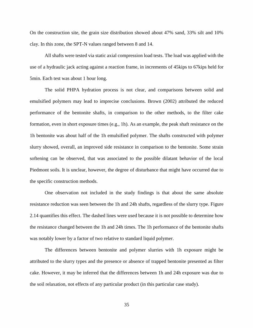
The solid PHPA hydration process is not clear, and comparisons between solid and

emulsified polymers may lead to imprecise conclusions. Brown (2002) attributed the reduced

performance of the bentonite shafts, in comparison to the other methods, to the filter cake

formation, even in short exposure times (e.g., 1h). As an example, the peak shaft resistance on the

1h bentonite was about half of the 1h emulsified polymer. The shafts constructed with polymer

slurry showed, overall, an improved side resistance in comparison to the bentonite. Some strain

softening can be observed, that was associated to the possible dilatant behavior of the local

Piedmont soils. It is unclear, however, the degree of disturbance that might have occurred due to

the specific construction methods.

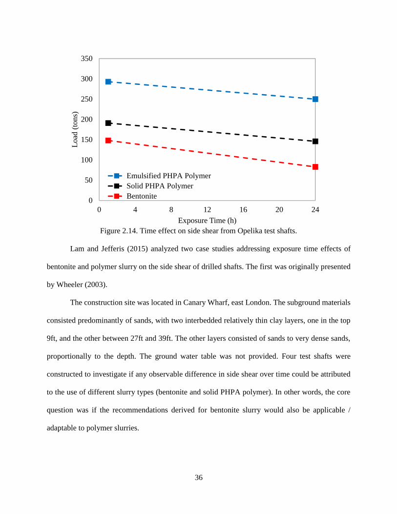
One observation not included in the study findings is that about the same absolute

resistance reduction was seen between the 1h and 24h shafts, regardless of the slurry type. Figure

2.14 quantifies this effect. The dashed lines were used because it is not possible to determine how

the resistance changed between the 1h and 24h times. The 1h performance of the bentonite shafts

was notably lower by a factor of two relative to standard liquid polymer.

The differences between bentonite and polymer slurries with 1h exposure might be

attributed to the slurry types and the presence or absence of trapped bentonite presented as filter

cake. However, it may be inferred that the differences between 1h and 24h exposure was due to

the soil relaxation, not effects of any particular product (in this particular case study).

36

Figure 2.14. Time effect on side shear from Opelika test shafts.

Lam and Jefferis (2015) analyzed two case studies addressing exposure time effects of

bentonite and polymer slurry on the side shear of drilled shafts. The first was originally presented

by Wheeler (2003).

The construction site was located in Canary Wharf, east London. The subground materials

consisted predominantly of sands, with two interbedded relatively thin clay layers, one in the top

9ft, and the other between 27ft and 39ft. The other layers consisted of sands to very dense sands,

proportionally to the depth. The ground water table was not provided. Four test shafts were

constructed to investigate if any observable difference in side shear over time could be attributed

to the use of different slurry types (bentonite and solid PHPA polymer). In other words, the core

question was if the recommendations derived for bentonite slurry would also be applicable /

adaptable to polymer slurries.

0

50

100

150

200

250

300

350

0 4 8 12 16 20 24

Loa

d (t

ons)

Exposure Time (h)

Emulsified PHPA PolymerSolid PHPA PolymerBentonite

37

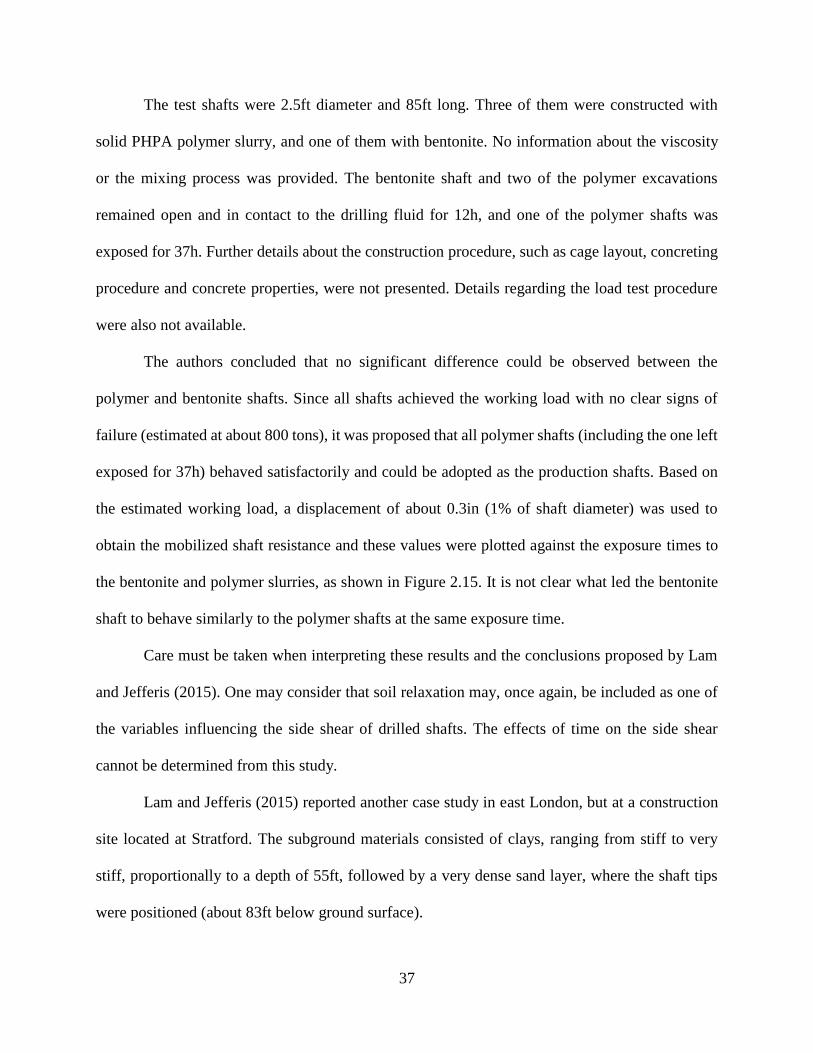
The test shafts were 2.5ft diameter and 85ft long. Three of them were constructed with

solid PHPA polymer slurry, and one of them with bentonite. No information about the viscosity

or the mixing process was provided. The bentonite shaft and two of the polymer excavations

remained open and in contact to the drilling fluid for 12h, and one of the polymer shafts was

exposed for 37h. Further details about the construction procedure, such as cage layout, concreting

procedure and concrete properties, were not presented. Details regarding the load test procedure

were also not available.

The authors concluded that no significant difference could be observed between the

polymer and bentonite shafts. Since all shafts achieved the working load with no clear signs of

failure (estimated at about 800 tons), it was proposed that all polymer shafts (including the one left

exposed for 37h) behaved satisfactorily and could be adopted as the production shafts. Based on

the estimated working load, a displacement of about 0.3in (1% of shaft diameter) was used to

obtain the mobilized shaft resistance and these values were plotted against the exposure times to

the bentonite and polymer slurries, as shown in Figure 2.15. It is not clear what led the bentonite

shaft to behave similarly to the polymer shafts at the same exposure time.

Care must be taken when interpreting these results and the conclusions proposed by Lam

and Jefferis (2015). One may consider that soil relaxation may, once again, be included as one of

the variables influencing the side shear of drilled shafts. The effects of time on the side shear

cannot be determined from this study.

Lam and Jefferis (2015) reported another case study in east London, but at a construction

site located at Stratford. The subground materials consisted of clays, ranging from stiff to very

stiff, proportionally to a depth of 55ft, followed by a very dense sand layer, where the shaft tips

were positioned (about 83ft below ground surface).

38

Figure 2.15. Effects of exposure time, Canary Wharf site.

Three 4ft diameter and 89ft long shafts were constructed, similarly to the Canary Wharf

case study, to investigate the influence of different drilling fluids and exposure times on the side

shear of drilled shafts. Two shafts were constructed with the aid of solid PHPA polymer slurry,

and one with bentonite slurry (same products as the Canary Wharf case study). The load vs

displacement curves are presented on Figure 2.16.

In this case, the polymer shafts outperformed bentonite. No appreciable difference could

be observed between the 7.5h and 26h exposure times to polymer slurry. Soil spatial variation

could be one of the variables, but no further information was provided that could explain these

results. Once again, the tests did not reach clear failure, and no means for computing the changes

in side shear were provided.

Lam and Jefferis (2015) concluded that, even under the working load, estimated to be about

1000 tons, no significant difference existed between the three shafts. No further discussions can

be properly proposed herein since the amount of available data is limited.

0

200

400

600

800

1000

1200

0 5 10 15 20 25 30 35 40

Loa

d (t

ons)

Exposure Time (h)

Polymer

Bentonite

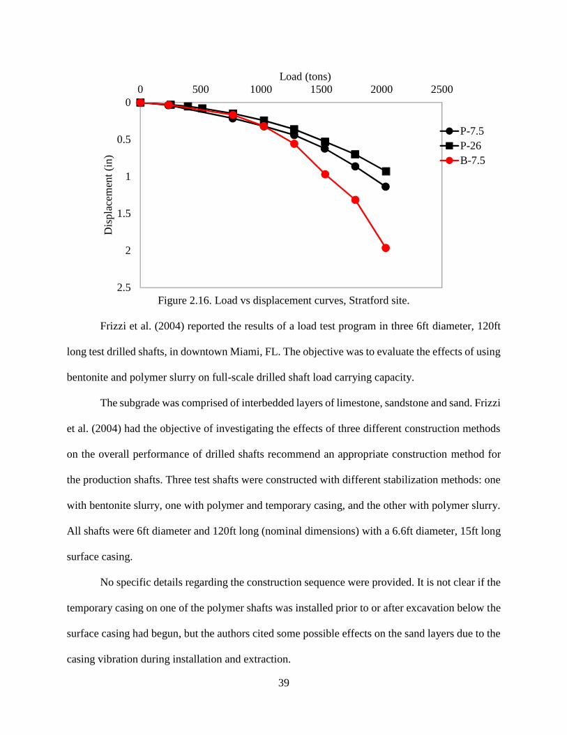
39

Figure 2.16. Load vs displacement curves, Stratford site.

Frizzi et al. (2004) reported the results of a load test program in three 6ft diameter, 120ft

long test drilled shafts, in downtown Miami, FL. The objective was to evaluate the effects of using

bentonite and polymer slurry on full-scale drilled shaft load carrying capacity.

The subgrade was comprised of interbedded layers of limestone, sandstone and sand. Frizzi

et al. (2004) had the objective of investigating the effects of three different construction methods

on the overall performance of drilled shafts recommend an appropriate construction method for

the production shafts. Three test shafts were constructed with different stabilization methods: one

with bentonite slurry, one with polymer and temporary casing, and the other with polymer slurry.

All shafts were 6ft diameter and 120ft long (nominal dimensions) with a 6.6ft diameter, 15ft long

surface casing.

No specific details regarding the construction sequence were provided. It is not clear if the

temporary casing on one of the polymer shafts was installed prior to or after excavation below the

surface casing had begun, but the authors cited some possible effects on the sand layers due to the

casing vibration during installation and extraction.

0

0.5

1

1.5

2

2.5

0 500 1000 1500 2000 2500

Dis

plac

emen

t (in

)

Load (tons)

P-7.5P-26B-7.5

40

All shafts were load tested by the use of O-cells. The results were presented in terms of

mobilized end bearing versus displacement and equivalent load on top versus displacement,

making possible to estimate the mobilized side resistance versus displacement for the three shafts

described by Frizzi et al. (2004). These inferred results are presented on Figure 2.17.

Figure 2.17. Estimated side shear resistance.

From Figure 2.17, the polymer shaft showed the best response in terms of side shear versus

displacement at side resistances below 6,000 kips, where the polymer-cased and the bentonite shaft

exhibited very similar results. At higher side resistance levels (beyond 8000 kips), the bentonite

shaft showed a better response. Based on the available information, explanations for these

differences and results do not seem appropriate.

Majano (1992) presented a series of small scale laboratory pull-out tests carried out on

model shafts constructed in sand, under different slurry types, concentrations and times of contact

with the soil. The lab model shafts were constructed in compacted sand, collected from the San

Jacinto River, which contained about 2% silt and clay. Five slurry product types were used in

various concentrations (viscosities) and different exposure times. The extraction cell reported by

Majano (1992) and Majano and O’Neill (1993) was designed to accommodate 3in diameter by

0

0.5

1

1.5

2

2.5

3

3.5

4

0 2000 4000 6000 8000 10000 12000

Dis

plac

emen

t (in

)

Load (kips)

Side Shear B

Side Shear P-C

Side Shear P

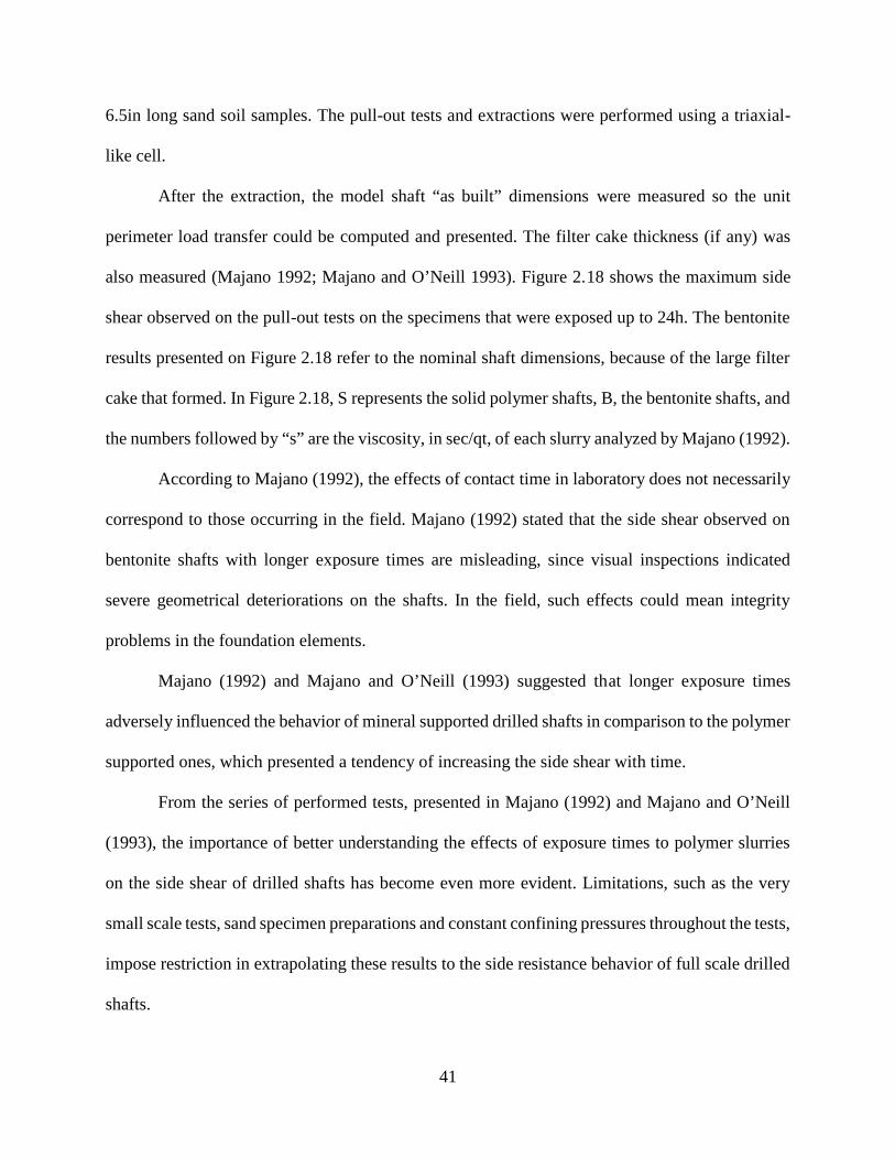
41

6.5in long sand soil samples. The pull-out tests and extractions were performed using a triaxial-

like cell.

After the extraction, the model shaft “as built” dimensions were measured so the unit

perimeter load transfer could be computed and presented. The filter cake thickness (if any) was

also measured (Majano 1992; Majano and O’Neill 1993). Figure 2.18 shows the maximum side

shear observed on the pull-out tests on the specimens that were exposed up to 24h. The bentonite

results presented on Figure 2.18 refer to the nominal shaft dimensions, because of the large filter

cake that formed. In Figure 2.18, S represents the solid polymer shafts, B, the bentonite shafts, and

the numbers followed by “s” are the viscosity, in sec/qt, of each slurry analyzed by Majano (1992).

According to Majano (1992), the effects of contact time in laboratory does not necessarily

correspond to those occurring in the field. Majano (1992) stated that the side shear observed on

bentonite shafts with longer exposure times are misleading, since visual inspections indicated

severe geometrical deteriorations on the shafts. In the field, such effects could mean integrity

problems in the foundation elements.

Majano (1992) and Majano and O’Neill (1993) suggested that longer exposure times

adversely influenced the behavior of mineral supported drilled shafts in comparison to the polymer

supported ones, which presented a tendency of increasing the side shear with time.

From the series of performed tests, presented in Majano (1992) and Majano and O’Neill

(1993), the importance of better understanding the effects of exposure times to polymer slurries

on the side shear of drilled shafts has become even more evident. Limitations, such as the very

small scale tests, sand specimen preparations and constant confining pressures throughout the tests,

impose restriction in extrapolating these results to the side resistance behavior of full scale drilled

shafts.

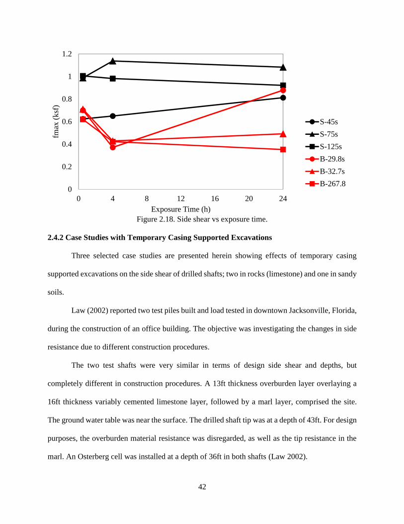
42

Figure 2.18. Side shear vs exposure time.

2.4.2 Case Studies with Temporary Casing Supported Excavations

Three selected case studies are presented herein showing effects of temporary casing

supported excavations on the side shear of drilled shafts; two in rocks (limestone) and one in sandy

soils.

Law (2002) reported two test piles built and load tested in downtown Jacksonville, Florida,

during the construction of an office building. The objective was investigating the changes in side

resistance due to different construction procedures.

The two test shafts were very similar in terms of design side shear and depths, but

completely different in construction procedures. A 13ft thickness overburden layer overlaying a

16ft thickness variably cemented limestone layer, followed by a marl layer, comprised the site.

The ground water table was near the surface. The drilled shaft tip was at a depth of 43ft. For design

purposes, the overburden material resistance was disregarded, as well as the tip resistance in the

marl. An Osterberg cell was installed at a depth of 36ft in both shafts (Law 2002).

0

0.2

0.4

0.6

0.8

1

1.2

0 4 8 12 16 20 24

fmax

(ks

f)

Exposure Time (h)

S-45s

S-75s

S-125s

B-29.8s

B-32.7s

B-267.8

43

In the first test shaft, an outer surface temporary casing, with outer diameter of 42.5in, was

installed with a vibratory hammer to the top of rock elevation, and an earth auger removed the

spoil from inside this casing. Next, a 15ft long, 36.75in outside diameter core barrel cored the

entire limestone layer at once. Then, a telescopic casing, with outer diameter of 36in, was placed

in the annular space excavated by the core barrel, and rotated into the marl formation. The rock

plug and the marl were drilled with a rock auger, the borehole was cleaned and the concrete was

poured by free fall (dry excavation). The temporary casings were extracted from outside-in (Law

2002).

In the second test shaft, the limestone was penetrated using a rock auger, which removed

the inner rock from the borehole during the excavation. The major difference was that the

temporary casings were extracted from the inside out.

The results of the load tests performed on the two test shafts were completely different. For

the first test shaft, the upper portion of the shaft failed in side shear when the applied O-cell load

reached around 205kips. For the second test shaft, no signs of failure were identified in the upper

portion up to the maximum applied O-cell load of around 1,220kips. Figure 2.19 shows the load

vs displacement curve for the two test shafts.

Law (2002) suggested that firstly extracting the outer casing could have caused degraded

materials to infuse into the annular space generated between the outer and inner casings, so

concrete could not establish bond with the excavated walls.

After the failure of the upper portion of test shaft in which the outer casing was extracted

first, no significant residual side shear could be observed. The displacement went back to zero by

the action of the upper shaft portion self-weight, estimated to be about 40kips. No information

about fluid concrete, cage or construction time was provided. Nonetheless, this extreme

44

discrepancy unquestionably emphasizes the importance of construction procedures on the side

shear of drilled shafts and its overall performance.

Figure 2.19. Load-displacement at top for test shafts in Jacksonville.

Castelli and Fan (2002) presented the results of load tests conducted in two drilled shafts

constructed with temporary casings into the limestone, during the replacement of the existing I-95

Fuller Warren Bridge over the St. Johns River in Jacksonville, Florida.

The bridge alignment was underlain by three formations, including overburden soils,

limestone, and marl. The limestone was found to be porous, weakly-cemented to well-cemented

(SPT N-values from less than 10 blows per foot to over 50/2 inches), having a thickness up to 20ft.

The top of the limestone stratum was typically encountered at elevations -15 to -35ft, and contained

interbedded seams of calcareous sand, silt, and clay, and was underlain by marl (Hawthorne

-5

-4

-3

-2

-1

0

1

2

0 200 400 600 800 1000 1200 1400

Dis

plac

emen

t (in

)

O-Cell Load (kips)

Outside-in, Upward

Outside-In, Downward

Inside-out, Upward

Inside-out, Downward

≈ 220kips

≈ 50kips

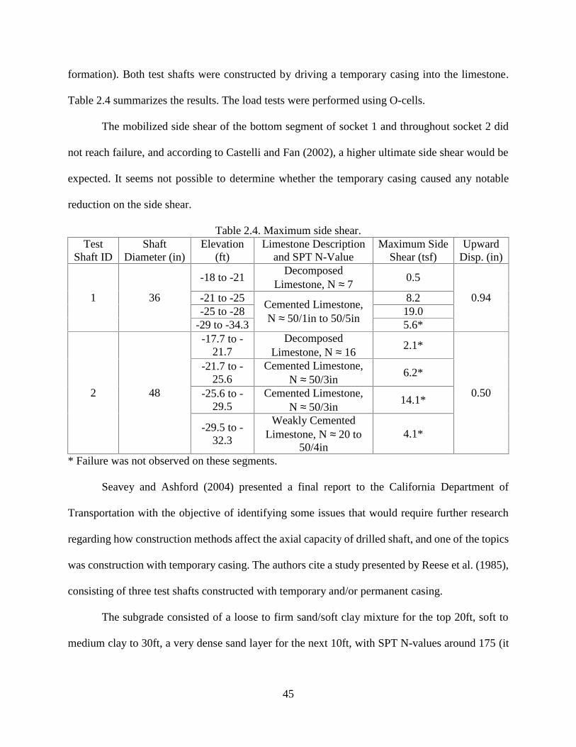
45

formation). Both test shafts were constructed by driving a temporary casing into the limestone.

Table 2.4 summarizes the results. The load tests were performed using O-cells.

The mobilized side shear of the bottom segment of socket 1 and throughout socket 2 did

not reach failure, and according to Castelli and Fan (2002), a higher ultimate side shear would be

expected. It seems not possible to determine whether the temporary casing caused any notable

reduction on the side shear.

Table 2.4. Maximum side shear.Test

Shaft IDShaft

Diameter (in)Elevation

(ft)Limestone Description

and SPT N-ValueMaximum Side

Shear (tsf)Upward

Disp. (in)

1 36

-18 to -21Decomposed

Limestone, N 70.5

0.94-21 to -25Cemented Limestone,N 50/1in to 50/5in

8.2-25 to -28 19.0

-29 to -34.3 5.6*

2 48

-17.7 to -21.7

DecomposedLimestone, N 16

2.1*

0.50

-21.7 to -25.6

Cemented Limestone,N 50/3in

6.2*

-25.6 to -29.5

Cemented Limestone,N 50/3in

14.1*

-29.5 to -32.3

Weakly CementedLimestone, N 20 to

50/4in4.1*

* Failure was not observed on these segments.

Seavey and Ashford (2004) presented a final report to the California Department of

Transportation with the objective of identifying some issues that would require further research

regarding how construction methods affect the axial capacity of drilled shaft, and one of the topics

was construction with temporary casing. The authors cite a study presented by Reese et al. (1985),

consisting of three test shafts constructed with temporary and/or permanent casing.

The subgrade consisted of a loose to firm sand/soft clay mixture for the top 20ft, soft to

medium clay to 30ft, a very dense sand layer for the next 10ft, with SPT N-values around 175 (it

46

is not clear why refusal was not noted). This dense sand layer was classified as an IGM and was

underlain by a soft to medium silty clay, with an undrained cohesive strength, su = 0.4tsf.

The first shaft was 60ft long and 48 inches diameter, constructed with temporary casing to

the depth of 52ft, and augering the soil from inside. The remaining length was excavated with

slurry, but the type of slurry was not provided. As the concrete was poured, the casing was

removed. This pile was chosen to be the control shaft. The second shaft was constructed with a

temporary 48 inch diameter casing that was driven to 50ft. The inner 36 inches were excavated

with slurry, and a permanent 36 inch diameter casing was placed inside the first casing and the

concrete poured. The third shaft used surface casing for the upper 10ft, and was excavated with

the slurry method for the remaining depth with a permanent 36 inch casing placed down to 40ft

(Reese et al. 1985), from Seavey and Ashford (2004).

Test shaft 1 showed the highest measured side shear among these three piles (Table 2.5).

The side resistance dropped significantly when permanent casing was installed, especially on test

shaft 2, where a combination of temporary and permanent casing was used in construction. In test

shaft 2, upon removal of the outer temporary casing, the soil experienced a significant relaxation

and possibly moved inward, indicating a void space between the pile and soil; thus, side resistance

was expected to be low. The ultimate side shear was estimated between 2.1 and 2.8tsf for the IGM

layer (Reese et al. 1985; Seavey and Ashford 2004). From these results, it is possible to infer that

constructing with temporary casing, and then extracting it, did not affect the side shear in

comparison with the designed / calculated values. No information regarding how the casings were

installed and extracted was presented.

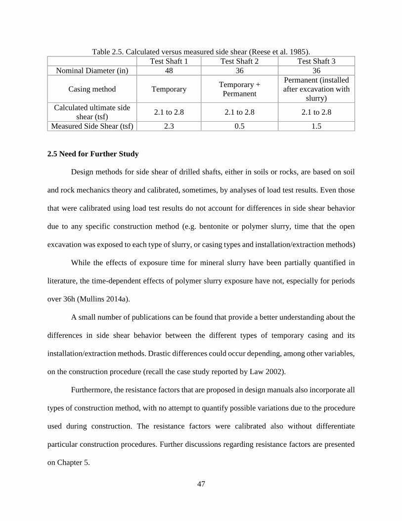
47

Table 2.5. Calculated versus measured side shear (Reese et al. 1985).Test Shaft 1 Test Shaft 2 Test Shaft 3

Nominal Diameter (in) 48 36 36

Casing method TemporaryTemporary +Permanent

Permanent (installedafter excavation with

slurry)Calculated ultimate side

shear (tsf)2.1 to 2.8 2.1 to 2.8 2.1 to 2.8

Measured Side Shear (tsf) 2.3 0.5 1.5

2.5 Need for Further Study

Design methods for side shear of drilled shafts, either in soils or rocks, are based on soil

and rock mechanics theory and calibrated, sometimes, by analyses of load test results. Even those

that were calibrated using load test results do not account for differences in side shear behavior

due to any specific construction method (e.g. bentonite or polymer slurry, time that the open

excavation was exposed to each type of slurry, or casing types and installation/extraction methods)

While the effects of exposure time for mineral slurry have been partially quantified in

literature, the time-dependent effects of polymer slurry exposure have not, especially for periods

over 36h (Mullins 2014a).

A small number of publications can be found that provide a better understanding about the

differences in side shear behavior between the different types of temporary casing and its

installation/extraction methods. Drastic differences could occur depending, among other variables,

on the construction procedure (recall the case study reported by Law 2002).

Furthermore, the resistance factors that are proposed in design manuals also incorporate all

types of construction method, with no attempt to quantify possible variations due to the procedure

used during construction. The resistance factors were calibrated also without differentiate

particular construction procedures. Further discussions regarding resistance factors are presented

on Chapter 5.

48

This research program provides evidence that the side shear behavior of drilled shafts in

sands and rock socketed shafts in limestone is influenced not only by the geotechnical properties

of the foundation geomaterial, but also by the construction procedures.

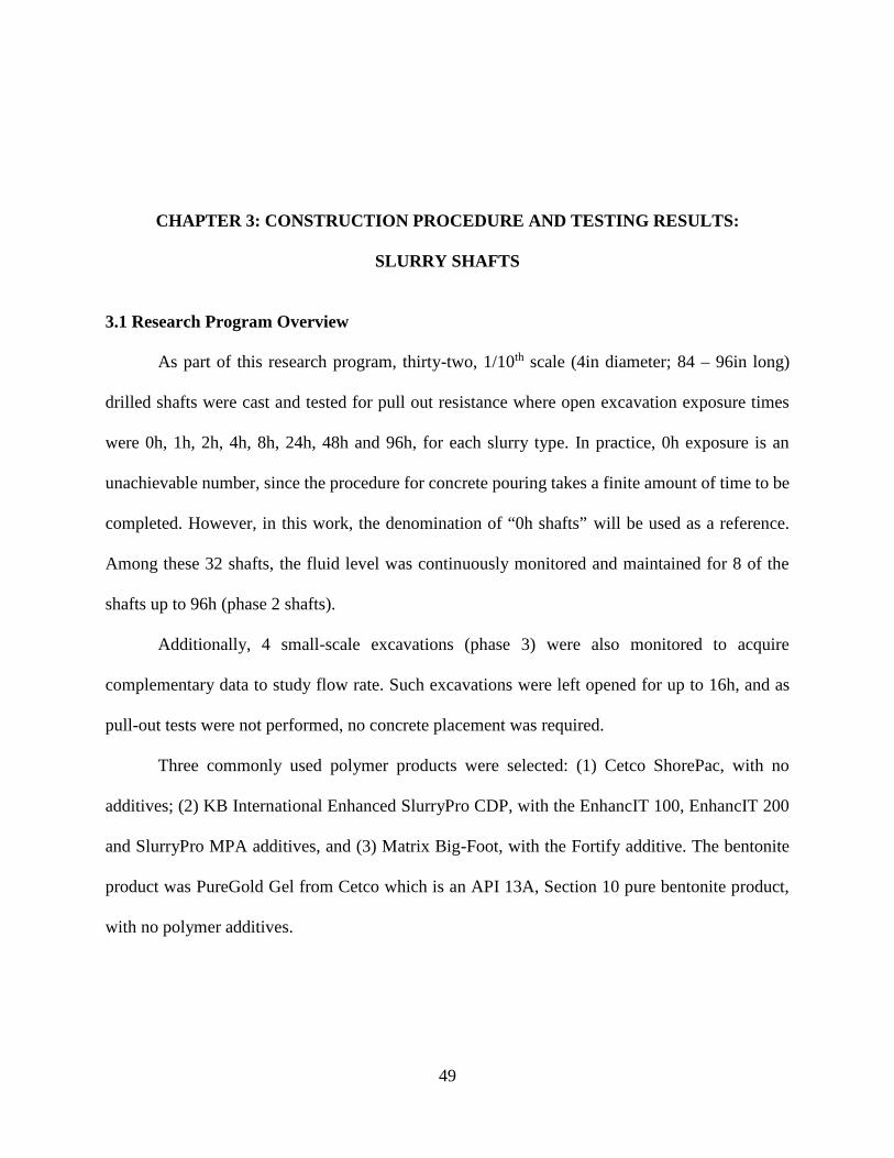
49

CHAPTER 3: CONSTRUCTION PROCEDURE AND TESTING RESULTS:

SLURRY SHAFTS

3.1 Research Program Overview

As part of this research program, thirty-two, 1/10th scale (4in diameter; 84 – 96in long)

drilled shafts were cast and tested for pull out resistance where open excavation exposure times

were 0h, 1h, 2h, 4h, 8h, 24h, 48h and 96h, for each slurry type. In practice, 0h exposure is an

unachievable number, since the procedure for concrete pouring takes a finite amount of time to be

completed. However, in this work, the denomination of “0h shafts” will be used as a reference.

Among these 32 shafts, the fluid level was continuously monitored and maintained for 8 of the

shafts up to 96h (phase 2 shafts).

Additionally, 4 small-scale excavations (phase 3) were also monitored to acquire

complementary data to study flow rate. Such excavations were left opened for up to 16h, and as

pull-out tests were not performed, no concrete placement was required.

Three commonly used polymer products were selected: (1) Cetco ShorePac, with no

additives; (2) KB International Enhanced SlurryPro CDP, with the EnhancIT 100, EnhancIT 200

and SlurryPro MPA additives, and (3) Matrix Big-Foot, with the Fortify additive. The bentonite

product was PureGold Gel from Cetco which is an API 13A, Section 10 pure bentonite product,

with no polymer additives.

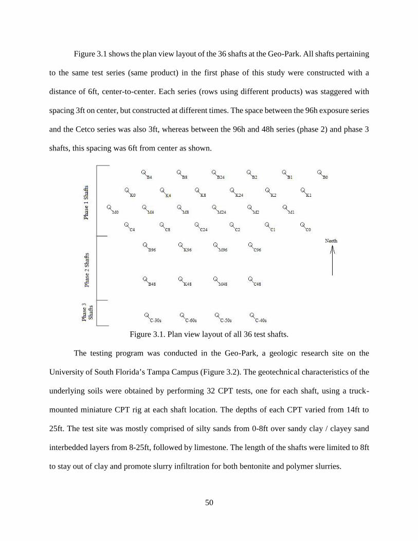
50

Figure 3.1 shows the plan view layout of the 36 shafts at the Geo-Park. All shafts pertaining

to the same test series (same product) in the first phase of this study were constructed with a

distance of 6ft, center-to-center. Each series (rows using different products) was staggered with

spacing 3ft on center, but constructed at different times. The space between the 96h exposure series

and the Cetco series was also 3ft, whereas between the 96h and 48h series (phase 2) and phase 3

shafts, this spacing was 6ft from center as shown.

Figure 3.1. Plan view layout of all 36 test shafts.

The testing program was conducted in the Geo-Park, a geologic research site on the

University of South Florida’s Tampa Campus (Figure 3.2). The geotechnical characteristics of the

underlying soils were obtained by performing 32 CPT tests, one for each shaft, using a truck-

mounted miniature CPT rig at each shaft location. The depths of each CPT varied from 14ft to

25ft. The test site was mostly comprised of silty sands from 0-8ft over sandy clay / clayey sand

interbedded layers from 8-25ft, followed by limestone. The length of the shafts were limited to 8ft

to stay out of clay and promote slurry infiltration for both bentonite and polymer slurries.

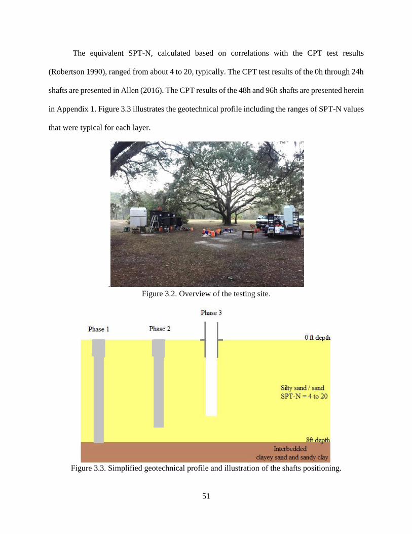
51

The equivalent SPT-N, calculated based on correlations with the CPT test results

(Robertson 1990), ranged from about 4 to 20, typically. The CPT test results of the 0h through 24h

shafts are presented in Allen (2016). The CPT results of the 48h and 96h shafts are presented herein

in Appendix 1. Figure 3.3 illustrates the geotechnical profile including the ranges of SPT-N values

that were typical for each layer.

.Figure 3.2. Overview of the testing site.

Figure 3.3. Simplified geotechnical profile and illustration of the shafts positioning.

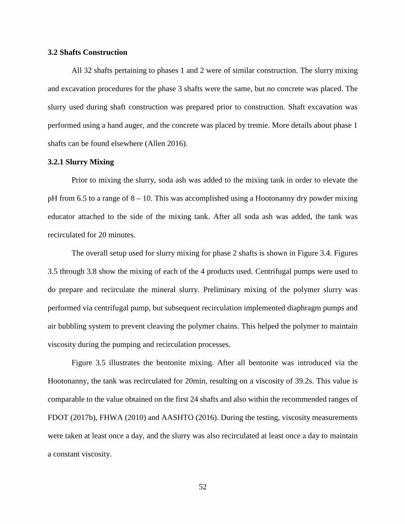
52

3.2 Shafts Construction

All 32 shafts pertaining to phases 1 and 2 were of similar construction. The slurry mixing

and excavation procedures for the phase 3 shafts were the same, but no concrete was placed. The

slurry used during shaft construction was prepared prior to construction. Shaft excavation was

performed using a hand auger, and the concrete was placed by tremie. More details about phase 1

shafts can be found elsewhere (Allen 2016).

3.2.1 Slurry Mixing

Prior to mixing the slurry, soda ash was added to the mixing tank in order to elevate the

pH from 6.5 to a range of 8 – 10. This was accomplished using a Hootonanny dry powder mixing

educator attached to the side of the mixing tank. After all soda ash was added, the tank was

recirculated for 20 minutes.

The overall setup used for slurry mixing for phase 2 shafts is shown in Figure 3.4. Figures

3.5 through 3.8 show the mixing of each of the 4 products used. Centrifugal pumps were used to

do prepare and recirculate the mineral slurry. Preliminary mixing of the polymer slurry was

performed via centrifugal pump, but subsequent recirculation implemented diaphragm pumps and

air bubbling system to prevent cleaving the polymer chains. This helped the polymer to maintain

viscosity during the pumping and recirculation processes.

Figure 3.5 illustrates the bentonite mixing. After all bentonite was introduced via the

Hootonanny, the tank was recirculated for 20min, resulting on a viscosity of 39.2s. This value is

comparable to the value obtained on the first 24 shafts and also within the recommended ranges of

FDOT (2017b), FHWA (2010) and AASHTO (2016). During the testing, viscosity measurements

were taken at least once a day, and the slurry was also recirculated at least once a day to maintain

a constant viscosity.

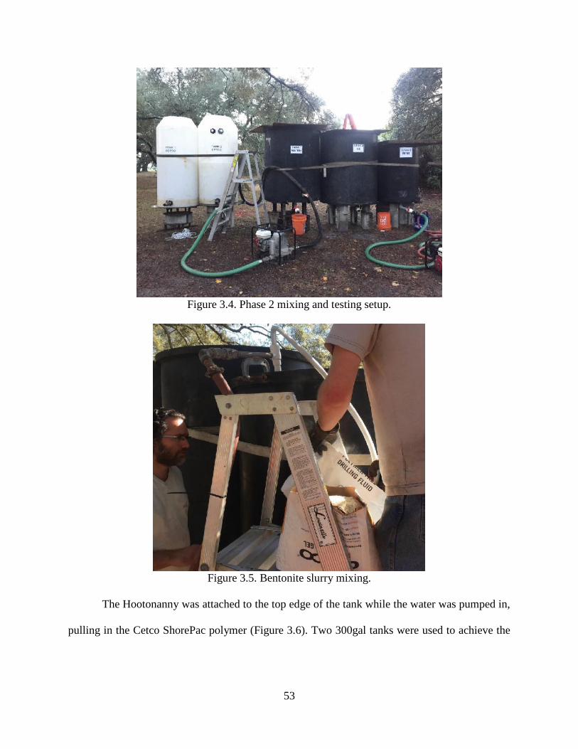
53

Figure 3.4. Phase 2 mixing and testing setup.

Figure 3.5. Bentonite slurry mixing.

The Hootonanny was attached to the top edge of the tank while the water was pumped in,

pulling in the Cetco ShorePac polymer (Figure 3.6). Two 300gal tanks were used to achieve the

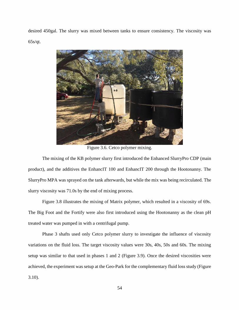
54

desired 450gal. The slurry was mixed between tanks to ensure consistency. The viscosity was

65s/qt.

Figure 3.6. Cetco polymer mixing.

The mixing of the KB polymer slurry first introduced the Enhanced SlurryPro CDP (main

product), and the additives the EnhancIT 100 and EnhancIT 200 through the Hootonanny. The

SlurryPro MPA was sprayed on the tank afterwards, but while the mix was being recirculated. The

slurry viscosity was 71.0s by the end of mixing process.

Figure 3.8 illustrates the mixing of Matrix polymer, which resulted in a viscosity of 69s.

The Big Foot and the Fortify were also first introduced using the Hootonanny as the clean pH

treated water was pumped in with a centrifugal pump.

Phase 3 shafts used only Cetco polymer slurry to investigate the influence of viscosity

variations on the fluid loss. The target viscosity values were 30s, 40s, 50s and 60s. The mixing

setup was similar to that used in phases 1 and 2 (Figure 3.9). Once the desired viscosities were

achieved, the experiment was setup at the Geo-Park for the complementary fluid loss study (Figure

3.10).

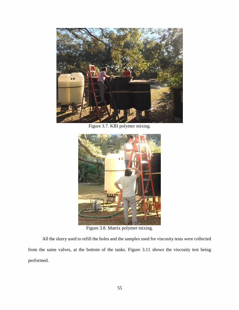
55

Figure 3.7. KBI polymer mixing.

Figure 3.8. Matrix polymer mixing.

All the slurry used to refill the holes and the samples used for viscosity tests were collected

from the same valves, at the bottom of the tanks. Figure 3.11 shows the viscosity test being

performed.

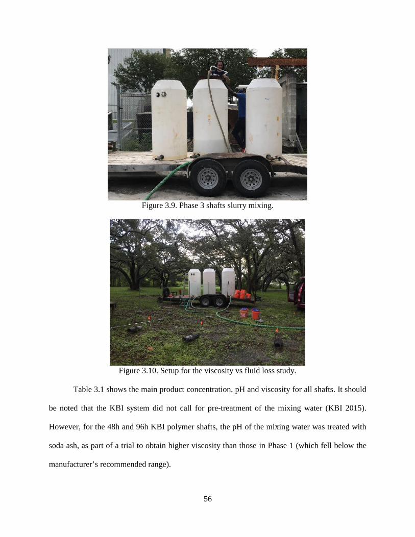
56

Figure 3.9. Phase 3 shafts slurry mixing.

Figure 3.10. Setup for the viscosity vs fluid loss study.

Table 3.1 shows the main product concentration, pH and viscosity for all shafts. It should

be noted that the KBI system did not call for pre-treatment of the mixing water (KBI 2015).

However, for the 48h and 96h KBI polymer shafts, the pH of the mixing water was treated with

soda ash, as part of a trial to obtain higher viscosity than those in Phase 1 (which fell below the

manufacturer’s recommended range).

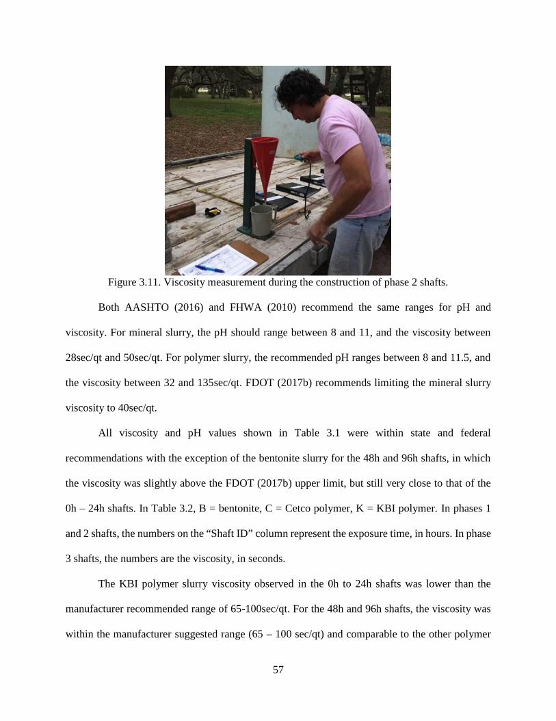
57

Figure 3.11. Viscosity measurement during the construction of phase 2 shafts.

Both AASHTO (2016) and FHWA (2010) recommend the same ranges for pH and

viscosity. For mineral slurry, the pH should range between 8 and 11, and the viscosity between

28sec/qt and 50sec/qt. For polymer slurry, the recommended pH ranges between 8 and 11.5, and

the viscosity between 32 and 135sec/qt. FDOT (2017b) recommends limiting the mineral slurry

viscosity to 40sec/qt.

All viscosity and pH values shown in Table 3.1 were within state and federal

recommendations with the exception of the bentonite slurry for the 48h and 96h shafts, in which

the viscosity was slightly above the FDOT (2017b) upper limit, but still very close to that of the

0h – 24h shafts. In Table 3.2, B = bentonite, C = Cetco polymer, K = KBI polymer. In phases 1

and 2 shafts, the numbers on the “Shaft ID” column represent the exposure time, in hours. In phase

3 shafts, the numbers are the viscosity, in seconds.

The KBI polymer slurry viscosity observed in the 0h to 24h shafts was lower than the

manufacturer recommended range of 65-100sec/qt. For the 48h and 96h shafts, the viscosity was

within the manufacturer suggested range (65 – 100 sec/qt) and comparable to the other polymer

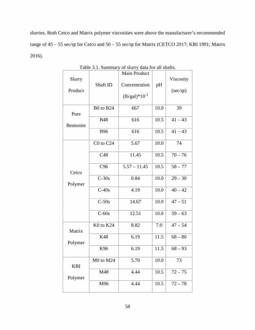
58

slurries. Both Cetco and Matrix polymer viscosities were above the manufacturer’s recommended

range of 45 – 55 sec/qt for Cetco and 50 – 55 sec/qt for Matrix (CETCO 2017; KBI 1991; Matrix

2016).

Table 3.1. Summary of slurry data for all shafts.

Slurry

ProductShaft ID

Main Product

Concentration

(lb/gal)*10-3

pHViscosity

(sec/qt)

Pure

Bentonite

B0 to B24 667 10.0 39

B48 616 10.5 41 – 43

B96 616 10.5 41 – 43

Cetco

Polymer

C0 to C24 5.67 10.0 74

C48 11.45 10.5 70 – 76

C96 5.57 – 11.45 10.5 58 – 77

C-30s 0.84 10.0 29 – 30

C-40s 4.19 10.0 40 – 42

C-50s 14.67 10.0 47 – 51

C-60s 12.51 10.0 59 – 63

Matrix

Polymer

K0 to K24 8.82 7.0 47 – 54

K48 6.19 11.5 68 – 80

K96 6.19 11.5 68 – 93

KBI

Polymer

M0 to M24 5.70 10.0 73

M48 4.44 10.5 72 – 75

M96 4.44 10.5 72 – 78

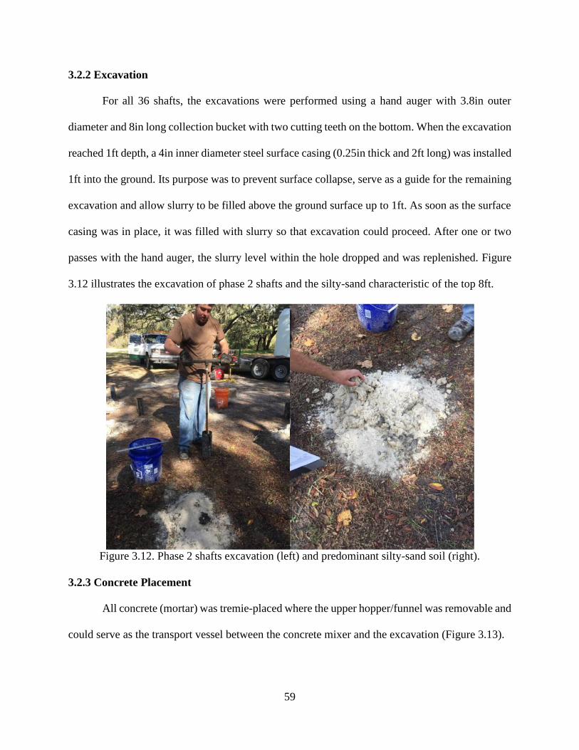
59

3.2.2 Excavation

For all 36 shafts, the excavations were performed using a hand auger with 3.8in outer

diameter and 8in long collection bucket with two cutting teeth on the bottom. When the excavation

reached 1ft depth, a 4in inner diameter steel surface casing (0.25in thick and 2ft long) was installed

1ft into the ground. Its purpose was to prevent surface collapse, serve as a guide for the remaining

excavation and allow slurry to be filled above the ground surface up to 1ft. As soon as the surface

casing was in place, it was filled with slurry so that excavation could proceed. After one or two

passes with the hand auger, the slurry level within the hole dropped and was replenished. Figure

3.12 illustrates the excavation of phase 2 shafts and the silty-sand characteristic of the top 8ft.

Figure 3.12. Phase 2 shafts excavation (left) and predominant silty-sand soil (right).

3.2.3 Concrete Placement

All concrete (mortar) was tremie-placed where the upper hopper/funnel was removable and

could serve as the transport vessel between the concrete mixer and the excavation (Figure 3.13).

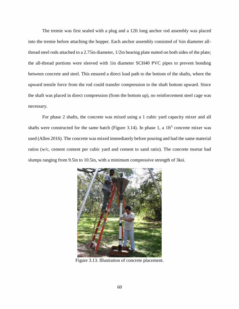
60

The tremie was first sealed with a plug and a 12ft long anchor rod assembly was placed

into the tremie before attaching the hopper. Each anchor assembly consisted of ¾in diameter all-

thread steel rods attached to a 2.75in diameter, 1/2in bearing plate nutted on both sides of the plate;

the all-thread portions were sleeved with 1in diameter SCH40 PVC pipes to prevent bonding

between concrete and steel. This ensured a direct load path to the bottom of the shafts, where the

upward tensile force from the rod could transfer compression to the shaft bottom upward. Since

the shaft was placed in direct compression (from the bottom up), no reinforcement steel cage was

necessary.

For phase 2 shafts, the concrete was mixed using a 1 cubic yard capacity mixer and all

shafts were constructed for the same batch (Figure 3.14). In phase 1, a 1ft3 concrete mixer was

used (Allen 2016). The concrete was mixed immediately before pouring and had the same material

ratios (w/c, cement content per cubic yard and cement to sand ratio). The concrete mortar had

slumps ranging from 9.5in to 10.5in, with a minimum compressive strength of 3ksi.

Figure 3.13. Illustration of concrete placement.

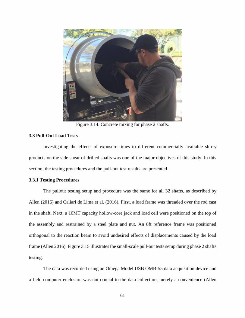
61

Figure 3.14. Concrete mixing for phase 2 shafts.

3.3 Pull-Out Load Tests

Investigating the effects of exposure times to different commercially available slurry

products on the side shear of drilled shafts was one of the major objectives of this study. In this

section, the testing procedures and the pull-out test results are presented.

3.3.1 Testing Procedures

The pullout testing setup and procedure was the same for all 32 shafts, as described by

Allen (2016) and Caliari de Lima et al. (2016). First, a load frame was threaded over the rod cast

in the shaft. Next, a 10MT capacity hollow-core jack and load cell were positioned on the top of

the assembly and restrained by a steel plate and nut. An 8ft reference frame was positioned

orthogonal to the reaction beam to avoid undesired effects of displacements caused by the load

frame (Allen 2016). Figure 3.15 illustrates the small-scale pull-out tests setup during phase 2 shafts

testing.

The data was recorded using an Omega Model USB OMB-55 data acquisition device and

a field computer enclosure was not crucial to the data collection, merely a convenience (Allen

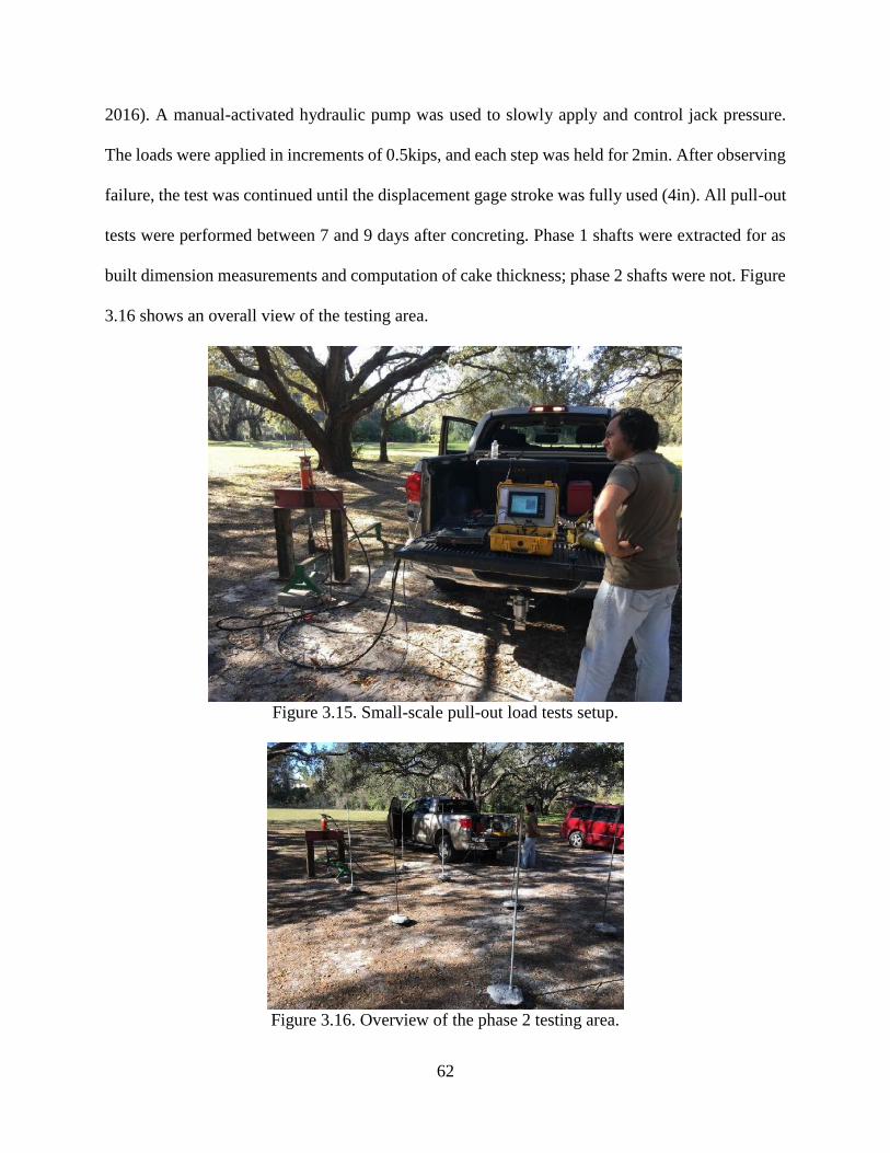
62

2016). A manual-activated hydraulic pump was used to slowly apply and control jack pressure.

The loads were applied in increments of 0.5kips, and each step was held for 2min. After observing

failure, the test was continued until the displacement gage stroke was fully used (4in). All pull-out

tests were performed between 7 and 9 days after concreting. Phase 1 shafts were extracted for as

built dimension measurements and computation of cake thickness; phase 2 shafts were not. Figure

3.16 shows an overall view of the testing area.

Figure 3.15. Small-scale pull-out load tests setup.

Figure 3.16. Overview of the phase 2 testing area.

63

3.3.2 Results

Figure 3.17 shows the field load vs displacement results for all 32 tested shafts, organized

by each set of products. In the legends, B denotes bentonite, C the Cetco polymer, K the KBI

polymer and M the Matrix polymer. Again, the numbers after the letters represent the exposure

time in hours.

When looking strictly at the pull-out load, the bentonite shafts were somewhat comparable

to polymer shafts for exposure times up to 4h. After longer exposure times, the polymer shafts

outperformed bentonite.

The maximum load achieved by the 96h bentonite shaft was about half of the 0h bentonite

shaft. This significant reduction on the maximum load can be associated with the filter cake

buildup over time (Allen 2016). Reductions due to longer exposure times were not observed in the

polymer shaft results. Majano (1992), Majano and O’Neill (1993) and Majano et al. (1994) also

reported similar observations.

Figures 3.18 and 3.19 show the variation of the maximum pull-out load and the side shear

resistance variations over time, respectively. The letter P on the legend represents the averaged

values for all three polymer products used. Again, little changes in the polymer performance were

noted; bentonite shafts showed almost a linear capacity loss with time after 4h.

Variations in both local soil strength and shaft dimensions can have an effect on the side

shear when comparing side-by-side load test results. Some variations are real, like shaft length,

and some are artificial, such as filter cake build up. Phase 1 shafts were exhumed and measured,

and smaller diameters caused by filter cake buildup after washing are not truly the correct

dimensions when computing side shear and, therefore, the actual failure surface was used which

included the filter cake thickness or the true sheared surface diameters (Allen 2016).

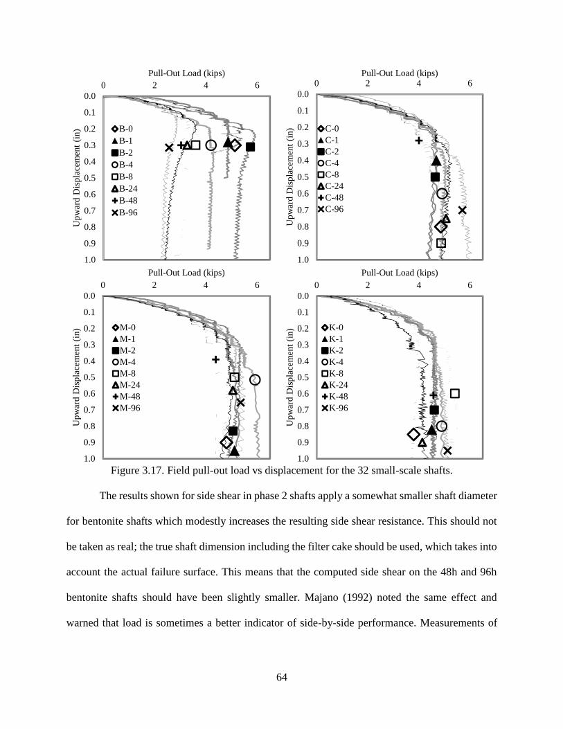
64

Figure 3.17. Field pull-out load vs displacement for the 32 small-scale shafts.

The results shown for side shear in phase 2 shafts apply a somewhat smaller shaft diameter

for bentonite shafts which modestly increases the resulting side shear resistance. This should not

be taken as real; the true shaft dimension including the filter cake should be used, which takes into

account the actual failure surface. This means that the computed side shear on the 48h and 96h

bentonite shafts should have been slightly smaller. Majano (1992) noted the same effect and

warned that load is sometimes a better indicator of side-by-side performance. Measurements of

0.0

0.1

0.2

0.3

0.4

0.5

0.6

0.7

0.8

0.9

1.0

0 2 4 6U

pwar

d D

ispl

acem

ent

(in)

Pull-Out Load (kips)

B-0B-1B-2B-4B-8B-24B-48B-96

0.0

0.1

0.2

0.3

0.4

0.5

0.6

0.7

0.8

0.9

1.0

0 2 4 6

Upw

ard

Dis

plac

emen

t (i

n)

Pull-Out Load (kips)

C-0C-1C-2C-4C-8C-24C-48C-96

0.0

0.1

0.2

0.3

0.4

0.5

0.6

0.7

0.8

0.9

1.0

0 2 4 6

Upw

ard

Dis

plac

emen

t (i

n)

Pull-Out Load (kips)

M-0M-1M-2M-4M-8M-24M-48M-96

0.0

0.1

0.2

0.3

0.4

0.5

0.6

0.7

0.8

0.9

1.0

0 2 4 6U

pwar

d D

ispl

acem

ent

(in)

Pull-Out Load (kips)

K-0K-1K-2K-4K-8K-24K-48K-96

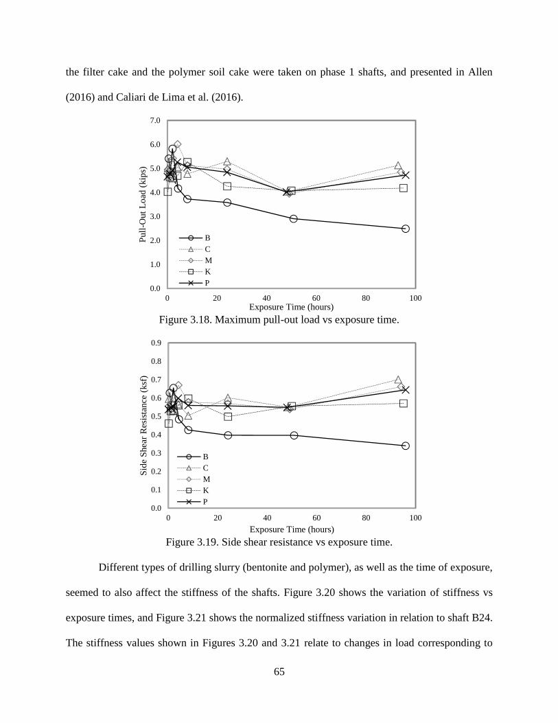
65

the filter cake and the polymer soil cake were taken on phase 1 shafts, and presented in Allen

(2016) and Caliari de Lima et al. (2016).

Figure 3.18. Maximum pull-out load vs exposure time.

Figure 3.19. Side shear resistance vs exposure time.

Different types of drilling slurry (bentonite and polymer), as well as the time of exposure,

seemed to also affect the stiffness of the shafts. Figure 3.20 shows the variation of stiffness vs

exposure times, and Figure 3.21 shows the normalized stiffness variation in relation to shaft B24.

The stiffness values shown in Figures 3.20 and 3.21 relate to changes in load corresponding to

0.0

1.0

2.0

3.0

4.0

5.0

6.0

7.0

0 20 40 60 80 100

Pul

l-O

ut L

oad

(kip

s)

Exposure Time (hours)

BCMKP

0.0

0.1

0.2

0.3

0.4

0.5

0.6

0.7

0.8

0.9

0 20 40 60 80 100

Side

She

ar R

esis

tanc

e (k

sf)

Exposure Time (hours)

BCMKP

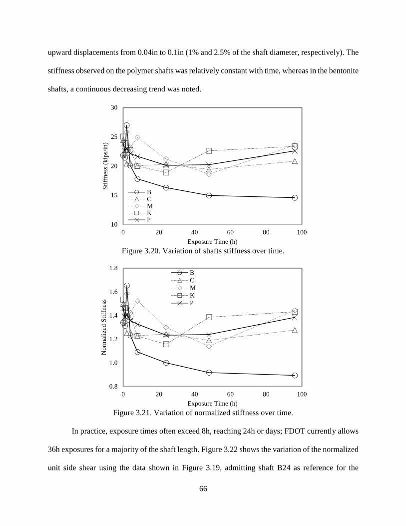
66

upward displacements from 0.04in to 0.1in (1% and 2.5% of the shaft diameter, respectively). The

stiffness observed on the polymer shafts was relatively constant with time, whereas in the bentonite

shafts, a continuous decreasing trend was noted.

Figure 3.20. Variation of shafts stiffness over time.

Figure 3.21. Variation of normalized stiffness over time.

In practice, exposure times often exceed 8h, reaching 24h or days; FDOT currently allows

36h exposures for a majority of the shaft length. Figure 3.22 shows the variation of the normalized

unit side shear using the data shown in Figure 3.19, admitting shaft B24 as reference for the

10

15

20

25

30

0 20 40 60 80 100

Stif

fnes

s (k

ips/

in)

Exposure Time (h)

BCMKP

0.8

1.0

1.2

1.4

1.6

1.8

0 20 40 60 80 100

Nor

mal

ized

Stif

fnes

s

Exposure Time (h)

BCMKP

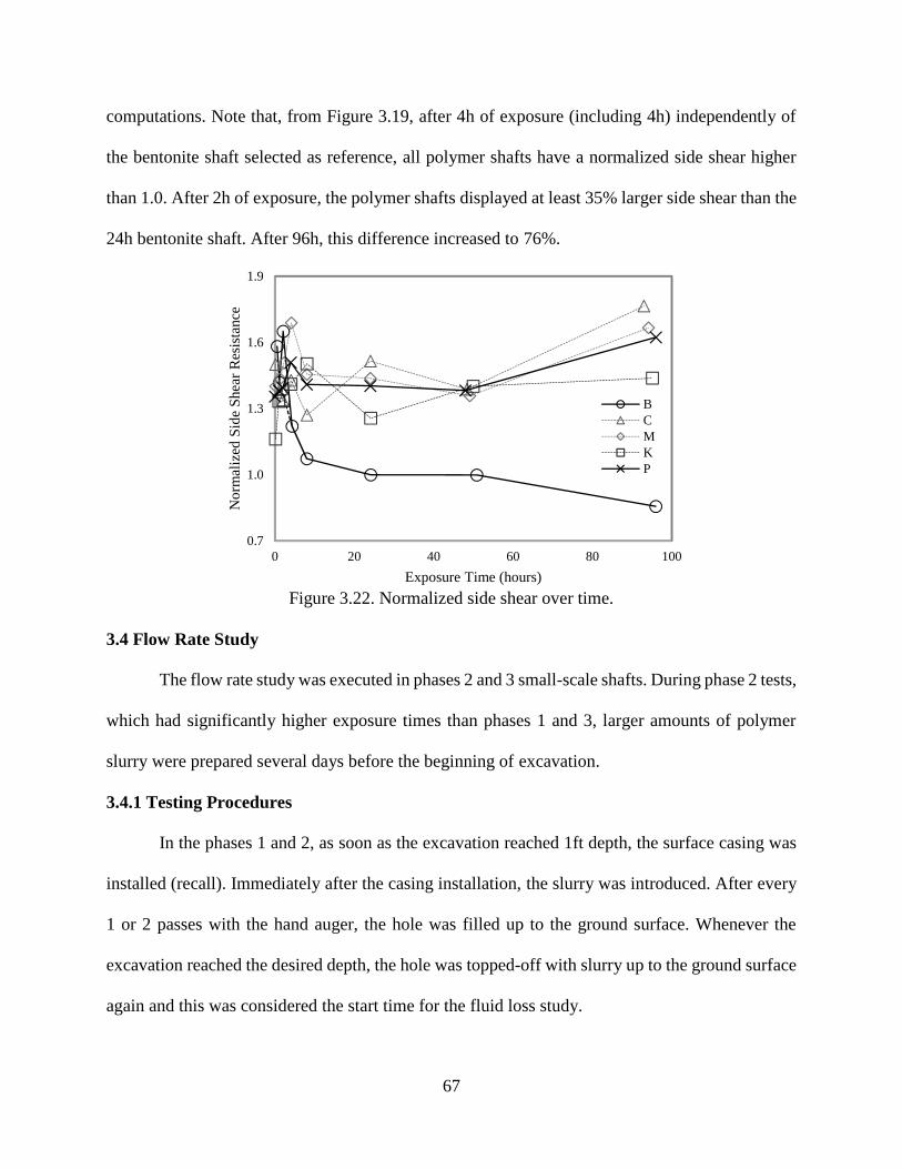
67

computations. Note that, from Figure 3.19, after 4h of exposure (including 4h) independently of

the bentonite shaft selected as reference, all polymer shafts have a normalized side shear higher

than 1.0. After 2h of exposure, the polymer shafts displayed at least 35% larger side shear than the

24h bentonite shaft. After 96h, this difference increased to 76%.

Figure 3.22. Normalized side shear over time.

3.4 Flow Rate Study

The flow rate study was executed in phases 2 and 3 small-scale shafts. During phase 2 tests,

which had significantly higher exposure times than phases 1 and 3, larger amounts of polymer

slurry were prepared several days before the beginning of excavation.

3.4.1 Testing Procedures

In the phases 1 and 2, as soon as the excavation reached 1ft depth, the surface casing was

installed (recall). Immediately after the casing installation, the slurry was introduced. After every

1 or 2 passes with the hand auger, the hole was filled up to the ground surface. Whenever the

excavation reached the desired depth, the hole was topped-off with slurry up to the ground surface

again and this was considered the start time for the fluid loss study.

0.7

1.0

1.3

1.6

1.9

0 20 40 60 80 100

Nor

mal

ized

Sid

e Sh

ear

Res

ista

nce

Exposure Time (hours)

BCMKP

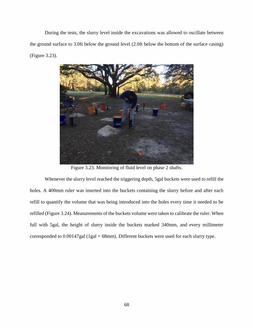
68

During the tests, the slurry level inside the excavations was allowed to oscillate between

the ground surface to 3.0ft below the ground level (2.0ft below the bottom of the surface casing)

(Figure 3.23).

Figure 3.23. Monitoring of fluid level on phase 2 shafts.

Whenever the slurry level reached the triggering depth, 5gal buckets were used to refill the

holes. A 400mm ruler was inserted into the buckets containing the slurry before and after each

refill to quantify the volume that was being introduced into the holes every time it needed to be

refilled (Figure 3.24). Measurements of the buckets volume were taken to calibrate the ruler. When

full with 5gal, the height of slurry inside the buckets marked 340mm, and every millimeter

corresponded to 0.00147gal (1gal = 68mm). Different buckets were used for each slurry type.

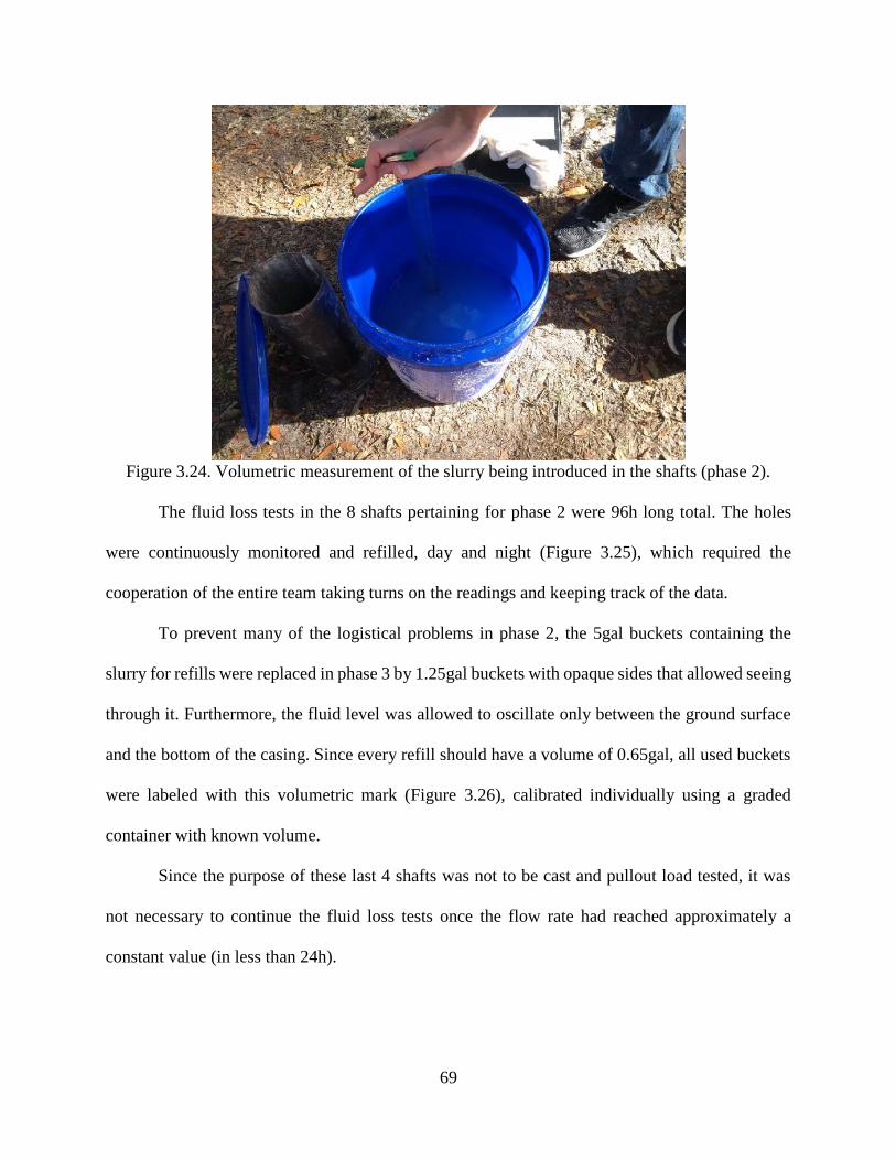
69

Figure 3.24. Volumetric measurement of the slurry being introduced in the shafts (phase 2).

The fluid loss tests in the 8 shafts pertaining for phase 2 were 96h long total. The holes

were continuously monitored and refilled, day and night (Figure 3.25), which required the

cooperation of the entire team taking turns on the readings and keeping track of the data.

To prevent many of the logistical problems in phase 2, the 5gal buckets containing the

slurry for refills were replaced in phase 3 by 1.25gal buckets with opaque sides that allowed seeing

through it. Furthermore, the fluid level was allowed to oscillate only between the ground surface

and the bottom of the casing. Since every refill should have a volume of 0.65gal, all used buckets

were labeled with this volumetric mark (Figure 3.26), calibrated individually using a graded

container with known volume.

Since the purpose of these last 4 shafts was not to be cast and pullout load tested, it was

not necessary to continue the fluid loss tests once the flow rate had reached approximately a

constant value (in less than 24h).

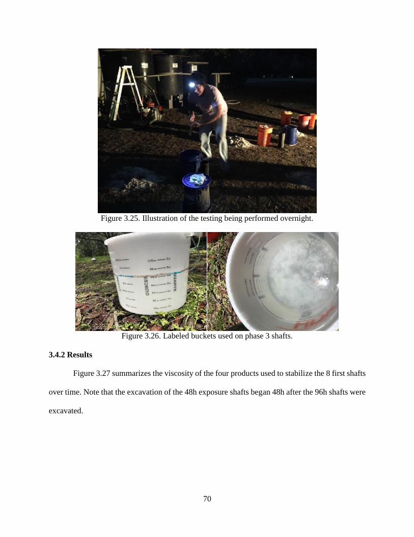
70

Figure 3.25. Illustration of the testing being performed overnight.

Figure 3.26. Labeled buckets used on phase 3 shafts.

3.4.2 Results

Figure 3.27 summarizes the viscosity of the four products used to stabilize the 8 first shafts

over time. Note that the excavation of the 48h exposure shafts began 48h after the 96h shafts were

excavated.

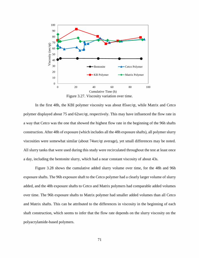
71

Figure 3.27. Viscosity variation over time.

In the first 48h, the KBI polymer viscosity was about 85sec/qt, while Matrix and Cetco

polymer displayed about 75 and 62sec/qt, respectively. This may have influenced the flow rate in

a way that Cetco was the one that showed the highest flow rate in the beginning of the 96h shafts

construction. After 48h of exposure (which includes all the 48h exposure shafts), all polymer slurry

viscosities were somewhat similar (about 74sec/qt average), yet small differences may be noted.

All slurry tanks that were used during this study were recirculated throughout the test at least once

a day, including the bentonite slurry, which had a near constant viscosity of about 43s.

Figure 3.28 shows the cumulative added slurry volume over time, for the 48h and 96h

exposure shafts. The 96h exposure shaft to the Cetco polymer had a clearly larger volume of slurry

added, and the 48h exposure shafts to Cetco and Matrix polymers had comparable added volumes

over time. The 96h exposure shafts to Matrix polymer had smaller added volumes than all Cetco

and Matrix shafts. This can be attributed to the differences in viscosity in the beginning of each

shaft construction, which seems to infer that the flow rate depends on the slurry viscosity on the

polyacrylamide-based polymers.

0

10

20

30

40

50

60

70

80

90

100

0 20 40 60 80 100

Vis

cosi

ty (

sec/

qt)

Cumulative Time (h)

Bentonite Cetco Polymer

KB Polymer Matrix Polymer

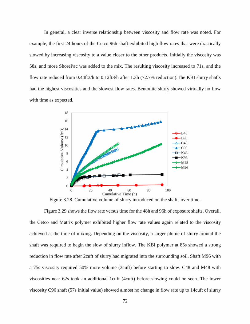
72

In general, a clear inverse relationship between viscosity and flow rate was noted. For

example, the first 24 hours of the Cetco 96h shaft exhibited high flow rates that were drastically

slowed by increasing viscosity to a value closer to the other products. Initially the viscosity was

58s, and more ShorePac was added to the mix. The resulting viscosity increased to 71s, and the

flow rate reduced from 0.44ft3/h to 0.12ft3/h after 1.3h (72.7% reduction).The KBI slurry shafts

had the highest viscosities and the slowest flow rates. Bentonite slurry showed virtually no flow

with time as expected.

Figure 3.28. Cumulative volume of slurry introduced on the shafts over time.

Figure 3.29 shows the flow rate versus time for the 48h and 96h of exposure shafts. Overall,

the Cetco and Matrix polymer exhibited higher flow rate values again related to the viscosity

achieved at the time of mixing. Depending on the viscosity, a larger plume of slurry around the

shaft was required to begin the slow of slurry inflow. The KBI polymer at 85s showed a strong

reduction in flow rate after 2cuft of slurry had migrated into the surrounding soil. Shaft M96 with

a 75s viscosity required 50% more volume (3cuft) before starting to slow. C48 and M48 with

viscosities near 62s took an additional 1cuft (4cuft) before slowing could be seen. The lower

viscosity C96 shaft (57s initial value) showed almost no change in flow rate up to 14cuft of slurry

0

2

4

6

8

10

12

14

16

18

0 20 40 60 80 100

Cum

ulat

ive

Vol

ume

(ft^

3)

Cumulative Time (h)

B48B96C48C96K48K96M48M96

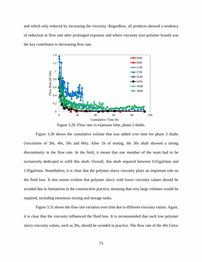
73

and which only reduced by increasing the viscosity. Regardless, all products showed a tendency

of reduction in flow rate after prolonged exposure and where viscosity (not polymer brand) was

the key contributor to decreasing flow rate.

Figure 3.29. Flow rate vs exposure time, phase 2 shafts.

Figure 3.30 shows the cumulative volume that was added over time for phase 3 shafts

(viscosities of 30s, 40s, 50s and 60s). After 1h of testing, the 30s shaft showed a strong

discontinuity in the flow rate. In the field, it meant that one member of the team had to be

exclusively dedicated to refill this shaft. Overall, this shaft required between 0.65gal/min and

1.95gal/min. Nonetheless, it is clear that the polymer slurry viscosity plays an important role on

the fluid loss. It also seems evident that polymer slurry with lower viscosity values should be

avoided due to limitations in the construction practice, meaning that very large volumes would be

required, including enormous mixing and storage tanks.

Figure 3.31 shows the flow rate variation over time due to different viscosity values. Again,

it is clear that the viscosity influenced the fluid loss. It is recommended that such low polymer

slurry viscosity values, such as 30s, should be avoided in practice. The flow rate of the 40s Cetco

0

0.2

0.4

0.6

0.8

1

1.2

1.4

0 20 40 60 80 100

Flow

Rat

e (f

t^3/

h)

Cumulative Time (h)

B48

B96

C48

C96

K48

K96

M48

M96

74

polymer slurry was 2.3 times larger the value observed on the 50s slurry after 4h of exposure, and

4.4 times larger than the 60s slurry after 4h of exposure.

Figure 3.30. Cumulative slurry volume over time for different viscosities.

Figure 3.31. Flow rate over time for different viscosities.

0

2

4

6

8

10

12

14

16

18

0 2 4 6 8 10 12 14 16

Cum

ulat

ive

volu

me

(ft^

3)

Time after excavation (h)

C-30sC-40sC-50sC-60s

0

2

4

6

8

10

12

14

16

18

0 2 4 6 8 10 12 14 16

Flow

Rat

e (f

t^3/

h)

Time after excavation (h)

C-30s

C-40s

C-50s

C-60s

75

CHAPTER 4: CONSTRUCTION PROCEDURE AND TESTING RESULTS:

ROCK SOCKETED SHAFTS

4.1 Research Program Overview

A total of 29 small scale rock sockets (nominally 4.6in to 4.8in diameter and 18in long)

were constructed. The sockets were excavated into different simulated limestone materials, using

different casing installation and extraction procedures. Among these sockets, 11 were selected to

be inspection holes (control specimens), in which the casings were extracted before concrete

placement and the open excavation was cleaned out with water and then inspected prior to

concreting. The intent of the control specimens was to set a baseline for comparisons between

temporarily cased and uncased construction conditions.

All sockets were pull-out tested with tension loads applied on sleeved anchor bars, which

extended to a bearing plate on the bottom of the excavation, subjecting the socket concrete to

compression (similar to what was performed with the small-scale slurry shafts). After extraction,

the dimensions of the sockets were determined on the observable failure surface.

4.2 Simulated Limestone Material

The search for representative simulated limestone materials was a challenge itself

involving over 200 unconfined compression test specimens prepared from 29 different mixes. All

mixes were cast using varying ratios of sand, coquina shells, calcium hydroxide, cement and water.

The simulated limestone mixes targeted strengths between 100psi and 600psi. Similarly, texture

and porosity needed to replicate the porous structure typical of natural Florida limestone.

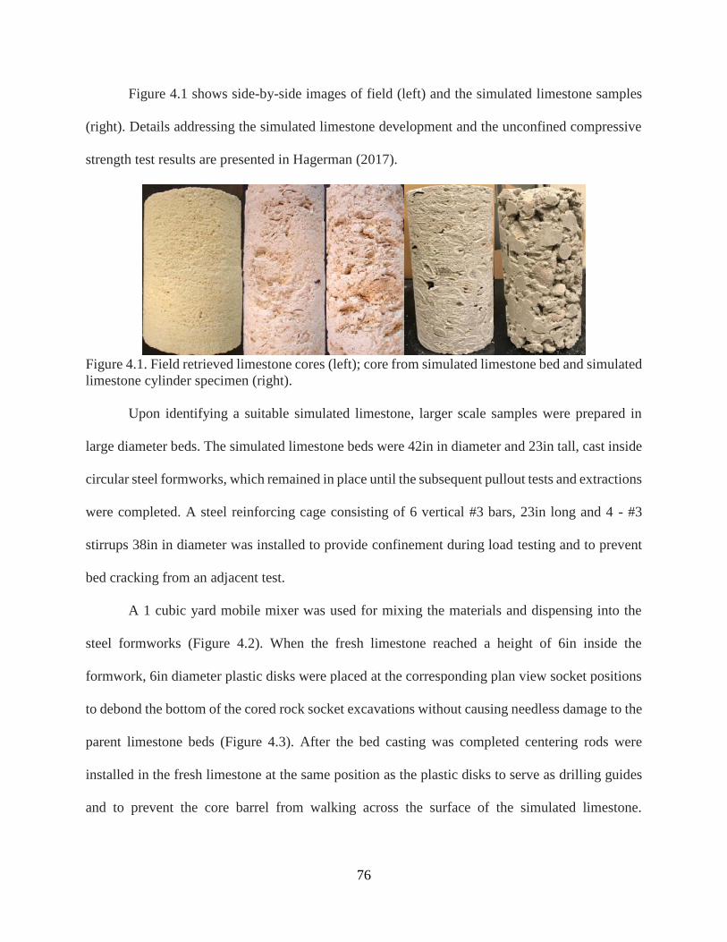
76

Figure 4.1 shows side-by-side images of field (left) and the simulated limestone samples

(right). Details addressing the simulated limestone development and the unconfined compressive

strength test results are presented in Hagerman (2017).

Figure 4.1. Field retrieved limestone cores (left); core from simulated limestone bed and simulatedlimestone cylinder specimen (right).

Upon identifying a suitable simulated limestone, larger scale samples were prepared in

large diameter beds. The simulated limestone beds were 42in in diameter and 23in tall, cast inside

circular steel formworks, which remained in place until the subsequent pullout tests and extractions

were completed. A steel reinforcing cage consisting of 6 vertical #3 bars, 23in long and 4 - #3

stirrups 38in in diameter was installed to provide confinement during load testing and to prevent

bed cracking from an adjacent test.

A 1 cubic yard mobile mixer was used for mixing the materials and dispensing into the

steel formworks (Figure 4.2). When the fresh limestone reached a height of 6in inside the

formwork, 6in diameter plastic disks were placed at the corresponding plan view socket positions

to debond the bottom of the cored rock socket excavations without causing needless damage to the

parent limestone beds (Figure 4.3). After the bed casting was completed centering rods were

installed in the fresh limestone at the same position as the plastic disks to serve as drilling guides

and to prevent the core barrel from walking across the surface of the simulated limestone.

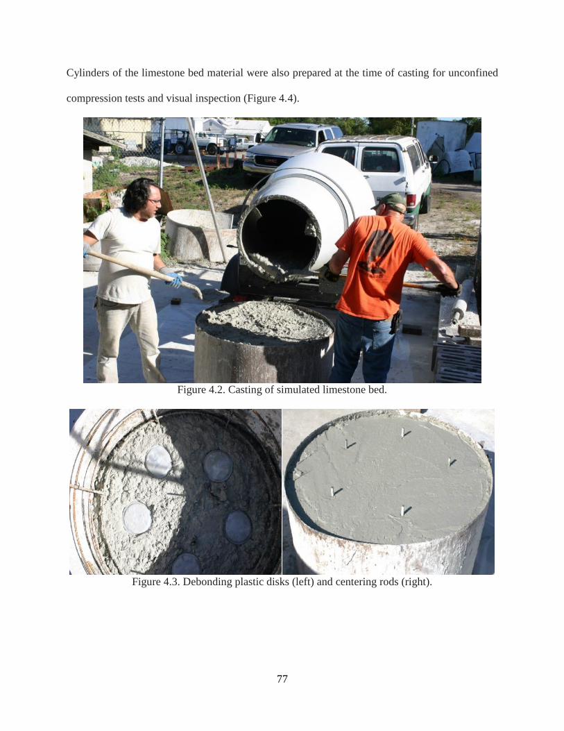
77

Cylinders of the limestone bed material were also prepared at the time of casting for unconfined

compression tests and visual inspection (Figure 4.4).

Figure 4.2. Casting of simulated limestone bed.

Figure 4.3. Debonding plastic disks (left) and centering rods (right).

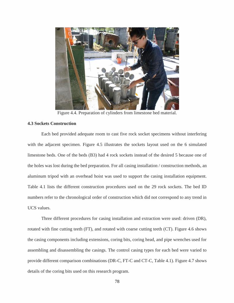
78

Figure 4.4. Preparation of cylinders from limestone bed material.

4.3 Sockets Construction

Each bed provided adequate room to cast five rock socket specimens without interfering

with the adjacent specimen. Figure 4.5 illustrates the sockets layout used on the 6 simulated

limestone beds. One of the beds (B3) had 4 rock sockets instead of the desired 5 because one of

the holes was lost during the bed preparation. For all casing installation / construction methods, an

aluminum tripod with an overhead hoist was used to support the casing installation equipment.

Table 4.1 lists the different construction procedures used on the 29 rock sockets. The bed ID

numbers refer to the chronological order of construction which did not correspond to any trend in

UCS values.

Three different procedures for casing installation and extraction were used: driven (DR),

rotated with fine cutting teeth (FT), and rotated with coarse cutting teeth (CT). Figure 4.6 shows

the casing components including extensions, coring bits, coring head, and pipe wrenches used for

assembling and disassembling the casings. The control casing types for each bed were varied to

provide different comparison combinations (DR-C, FT-C and CT-C, Table 4.1). Figure 4.7 shows

details of the coring bits used on this research program.

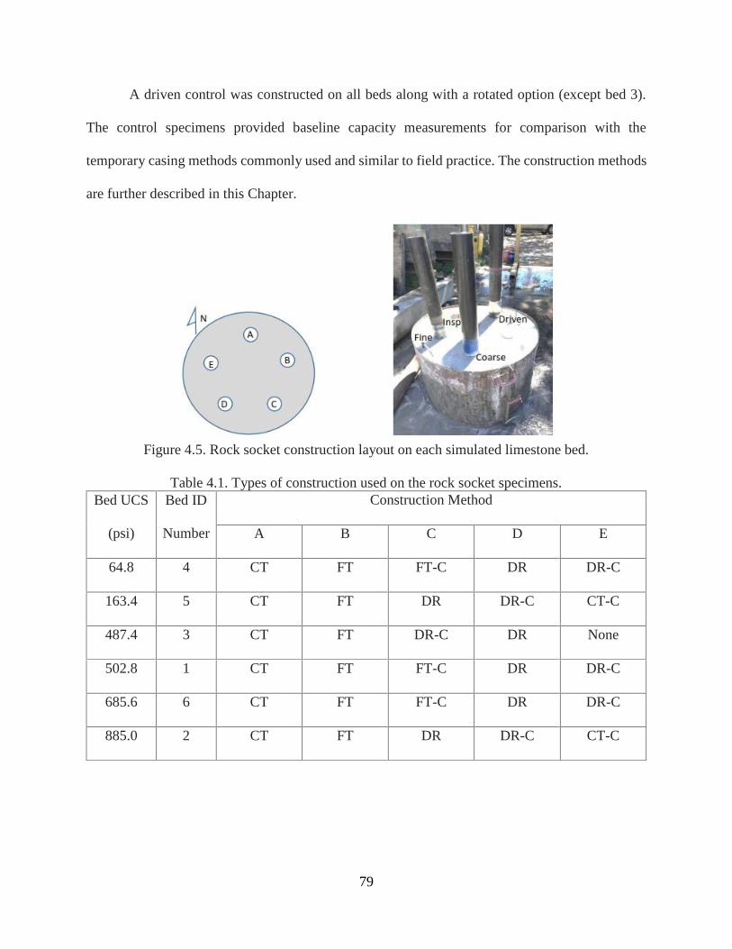
79

A driven control was constructed on all beds along with a rotated option (except bed 3).

The control specimens provided baseline capacity measurements for comparison with the

temporary casing methods commonly used and similar to field practice. The construction methods

are further described in this Chapter.

Figure 4.5. Rock socket construction layout on each simulated limestone bed.

Table 4.1. Types of construction used on the rock socket specimens.Bed UCS

(psi)

Bed ID

Number

Construction Method

A B C D E

64.8 4 CT FT FT-C DR DR-C

163.4 5 CT FT DR DR-C CT-C

487.4 3 CT FT DR-C DR None

502.8 1 CT FT FT-C DR DR-C

685.6 6 CT FT FT-C DR DR-C

885.0 2 CT FT DR DR-C CT-C

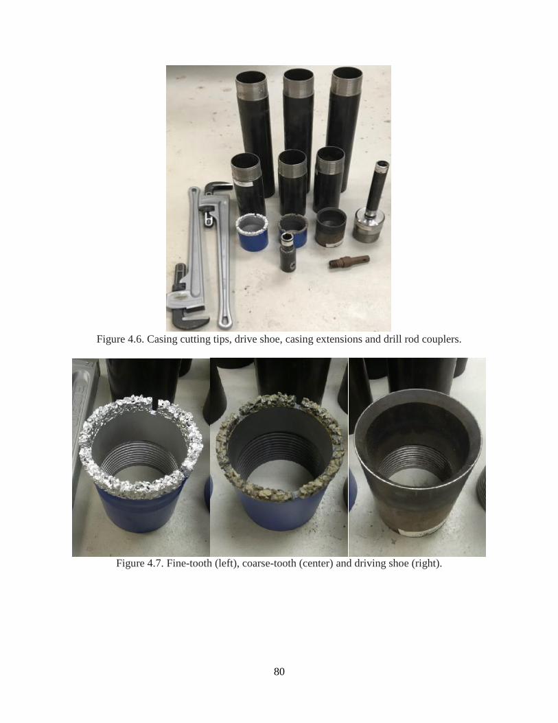
80

Figure 4.6. Casing cutting tips, drive shoe, casing extensions and drill rod couplers.

Figure 4.7. Fine-tooth (left), coarse-tooth (center) and driving shoe (right).

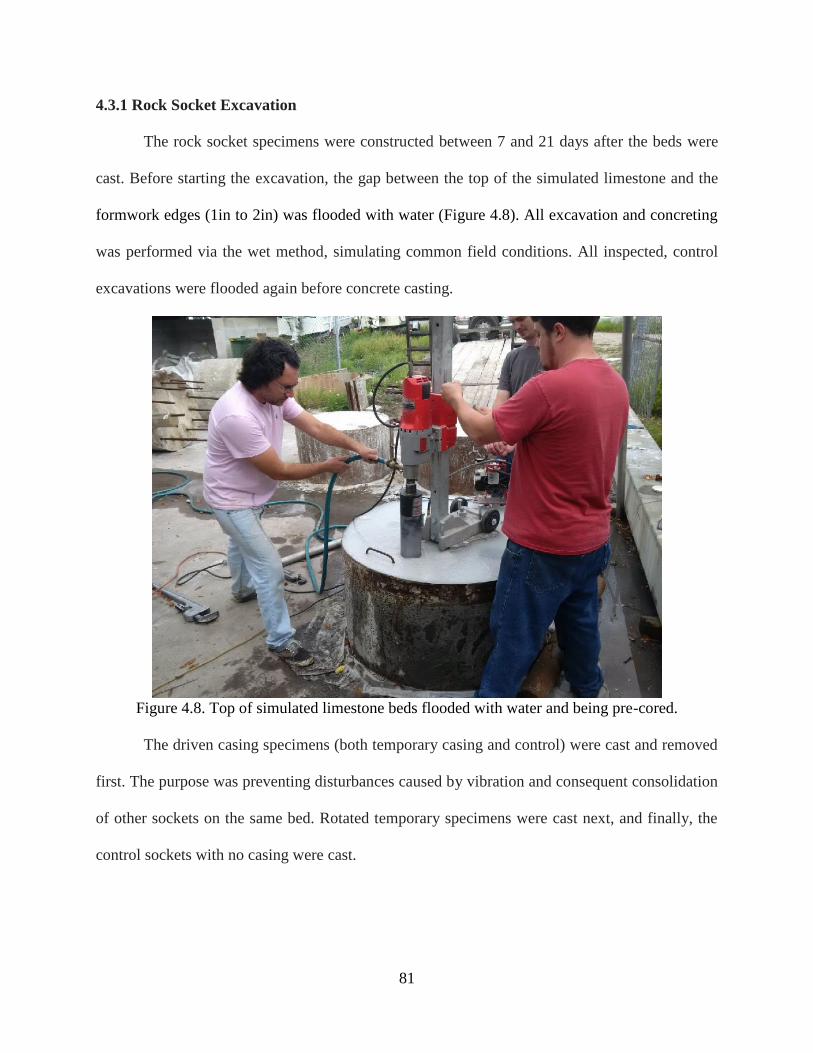
81

4.3.1 Rock Socket Excavation

The rock socket specimens were constructed between 7 and 21 days after the beds were

cast. Before starting the excavation, the gap between the top of the simulated limestone and the

formwork edges (1in to 2in) was flooded with water (Figure 4.8). All excavation and concreting

was performed via the wet method, simulating common field conditions. All inspected, control

excavations were flooded again before concrete casting.

Figure 4.8. Top of simulated limestone beds flooded with water and being pre-cored.

The driven casing specimens (both temporary casing and control) were cast and removed

first. The purpose was preventing disturbances caused by vibration and consequent consolidation

of other sockets on the same bed. Rotated temporary specimens were cast next, and finally, the

control sockets with no casing were cast.

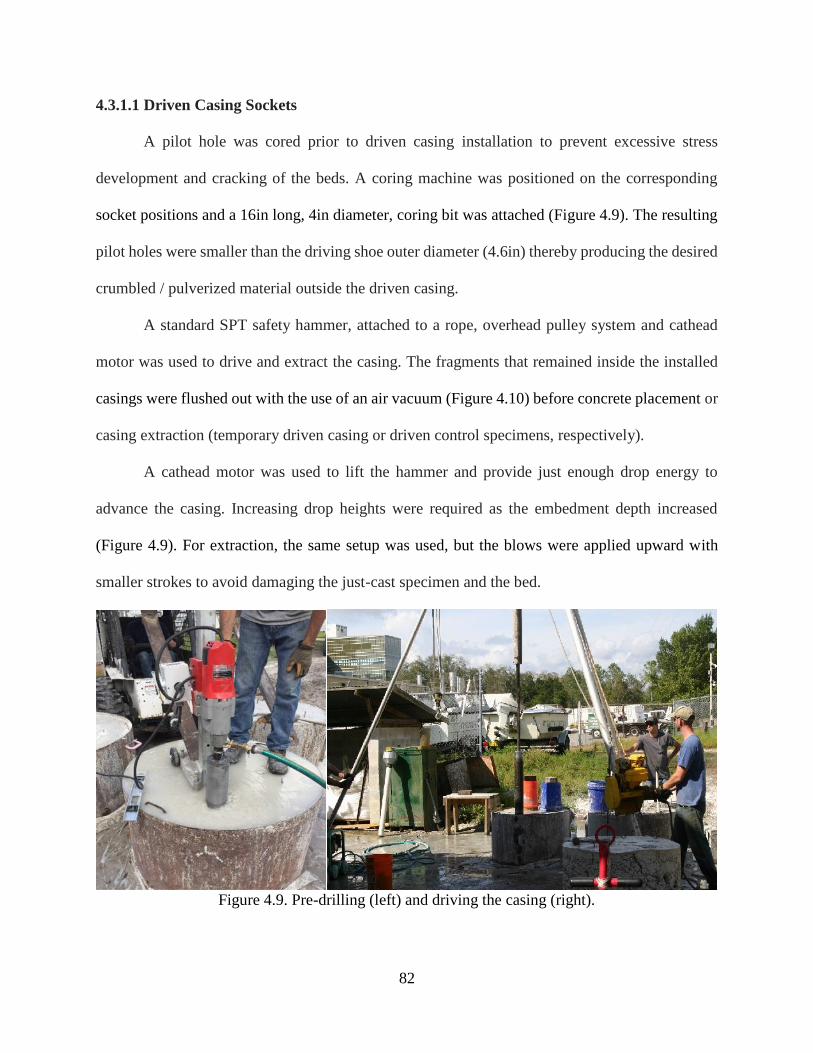
82

4.3.1.1 Driven Casing Sockets

A pilot hole was cored prior to driven casing installation to prevent excessive stress

development and cracking of the beds. A coring machine was positioned on the corresponding

socket positions and a 16in long, 4in diameter, coring bit was attached (Figure 4.9). The resulting

pilot holes were smaller than the driving shoe outer diameter (4.6in) thereby producing the desired

crumbled / pulverized material outside the driven casing.

A standard SPT safety hammer, attached to a rope, overhead pulley system and cathead

motor was used to drive and extract the casing. The fragments that remained inside the installed

casings were flushed out with the use of an air vacuum (Figure 4.10) before concrete placement or

casing extraction (temporary driven casing or driven control specimens, respectively).

A cathead motor was used to lift the hammer and provide just enough drop energy to

advance the casing. Increasing drop heights were required as the embedment depth increased

(Figure 4.9). For extraction, the same setup was used, but the blows were applied upward with

smaller strokes to avoid damaging the just-cast specimen and the bed.

Figure 4.9. Pre-drilling (left) and driving the casing (right).

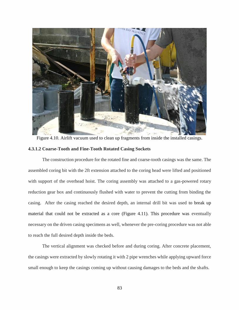
83

Figure 4.10. Airlift vacuum used to clean up fragments from inside the installed casings.

4.3.1.2 Coarse-Tooth and Fine-Tooth Rotated Casing Sockets

The construction procedure for the rotated fine and coarse-tooth casings was the same. The

assembled coring bit with the 2ft extension attached to the coring head were lifted and positioned

with support of the overhead hoist. The coring assembly was attached to a gas-powered rotary

reduction gear box and continuously flushed with water to prevent the cutting from binding the

casing. After the casing reached the desired depth, an internal drill bit was used to break up

material that could not be extracted as a core (Figure 4.11). This procedure was eventually

necessary on the driven casing specimens as well, whenever the pre-coring procedure was not able

to reach the full desired depth inside the beds.

The vertical alignment was checked before and during coring. After concrete placement,

the casings were extracted by slowly rotating it with 2 pipe wrenches while applying upward force

small enough to keep the casings coming up without causing damages to the beds and the shafts.

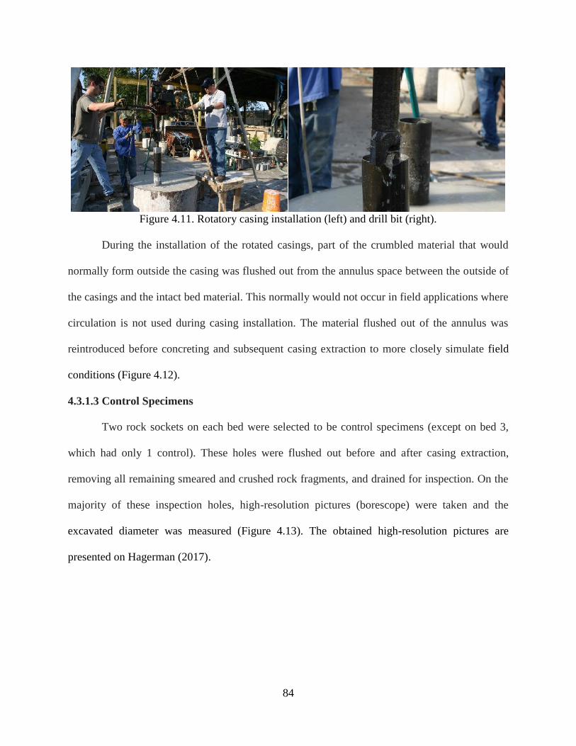
84

Figure 4.11. Rotatory casing installation (left) and drill bit (right).

During the installation of the rotated casings, part of the crumbled material that would

normally form outside the casing was flushed out from the annulus space between the outside of

the casings and the intact bed material. This normally would not occur in field applications where

circulation is not used during casing installation. The material flushed out of the annulus was

reintroduced before concreting and subsequent casing extraction to more closely simulate field

conditions (Figure 4.12).

4.3.1.3 Control Specimens

Two rock sockets on each bed were selected to be control specimens (except on bed 3,

which had only 1 control). These holes were flushed out before and after casing extraction,

removing all remaining smeared and crushed rock fragments, and drained for inspection. On the

majority of these inspection holes, high-resolution pictures (borescope) were taken and the

excavated diameter was measured (Figure 4.13). The obtained high-resolution pictures are

presented on Hagerman (2017).

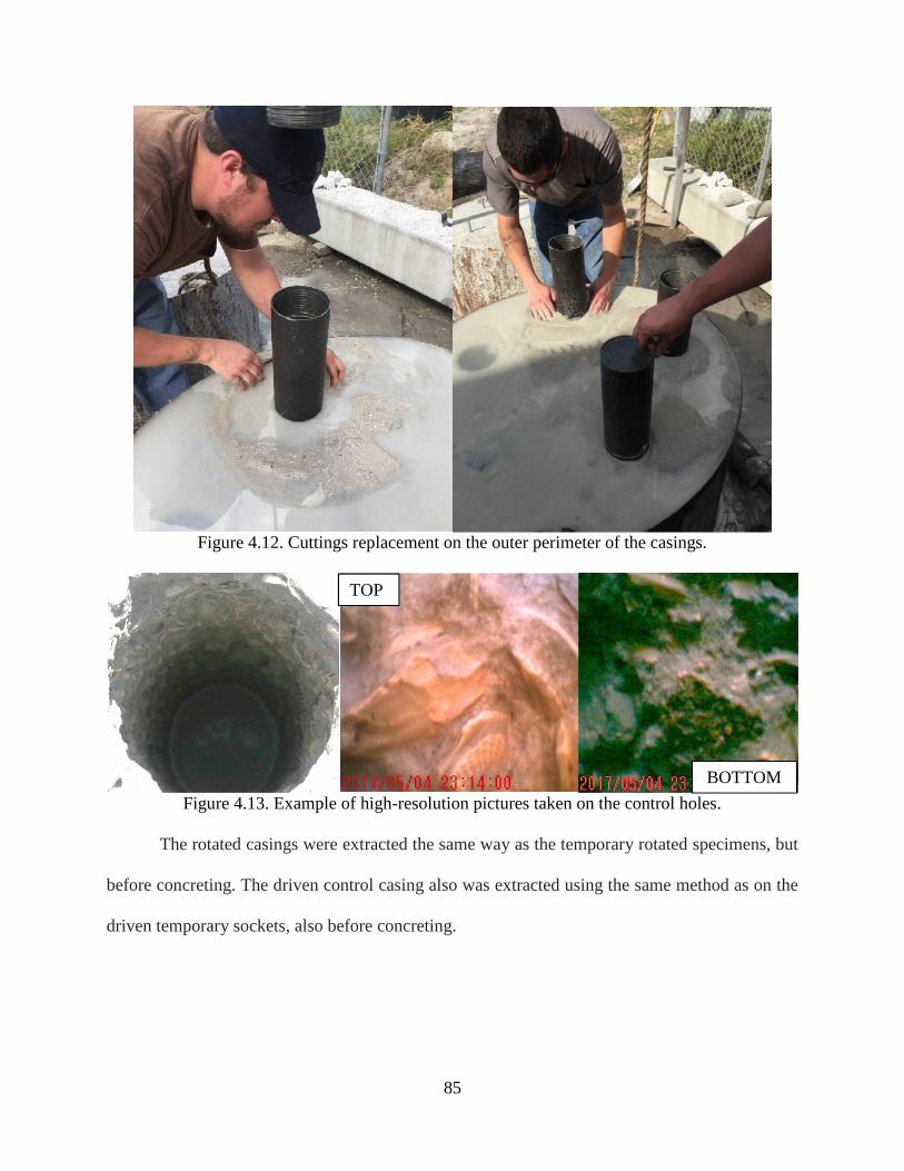
85

Figure 4.12. Cuttings replacement on the outer perimeter of the casings.

Figure 4.13. Example of high-resolution pictures taken on the control holes.

The rotated casings were extracted the same way as the temporary rotated specimens, but

before concreting. The driven control casing also was extracted using the same method as on the

driven temporary sockets, also before concreting.

TOP

BOTTOM

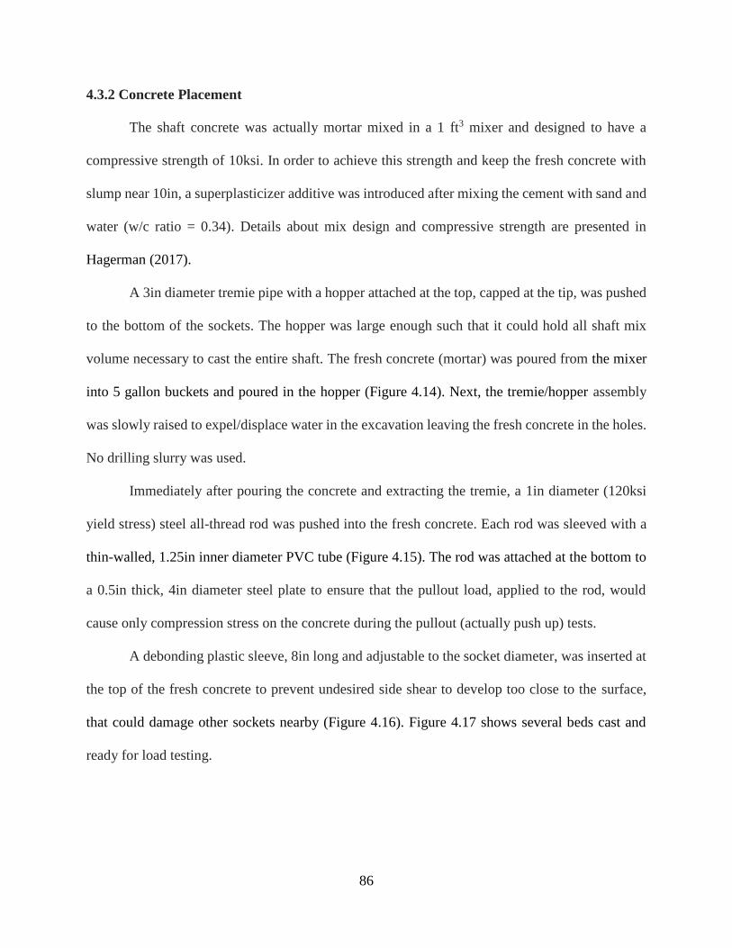
86

4.3.2 Concrete Placement

The shaft concrete was actually mortar mixed in a 1 ft3 mixer and designed to have a

compressive strength of 10ksi. In order to achieve this strength and keep the fresh concrete with

slump near 10in, a superplasticizer additive was introduced after mixing the cement with sand and

water (w/c ratio = 0.34). Details about mix design and compressive strength are presented in

Hagerman (2017).

A 3in diameter tremie pipe with a hopper attached at the top, capped at the tip, was pushed

to the bottom of the sockets. The hopper was large enough such that it could hold all shaft mix

volume necessary to cast the entire shaft. The fresh concrete (mortar) was poured from the mixer

into 5 gallon buckets and poured in the hopper (Figure 4.14). Next, the tremie/hopper assembly

was slowly raised to expel/displace water in the excavation leaving the fresh concrete in the holes.

No drilling slurry was used.

Immediately after pouring the concrete and extracting the tremie, a 1in diameter (120ksi

yield stress) steel all-thread rod was pushed into the fresh concrete. Each rod was sleeved with a

thin-walled, 1.25in inner diameter PVC tube (Figure 4.15). The rod was attached at the bottom to

a 0.5in thick, 4in diameter steel plate to ensure that the pullout load, applied to the rod, would

cause only compression stress on the concrete during the pullout (actually push up) tests.

A debonding plastic sleeve, 8in long and adjustable to the socket diameter, was inserted at

the top of the fresh concrete to prevent undesired side shear to develop too close to the surface,

that could damage other sockets nearby (Figure 4.16). Figure 4.17 shows several beds cast and

ready for load testing.

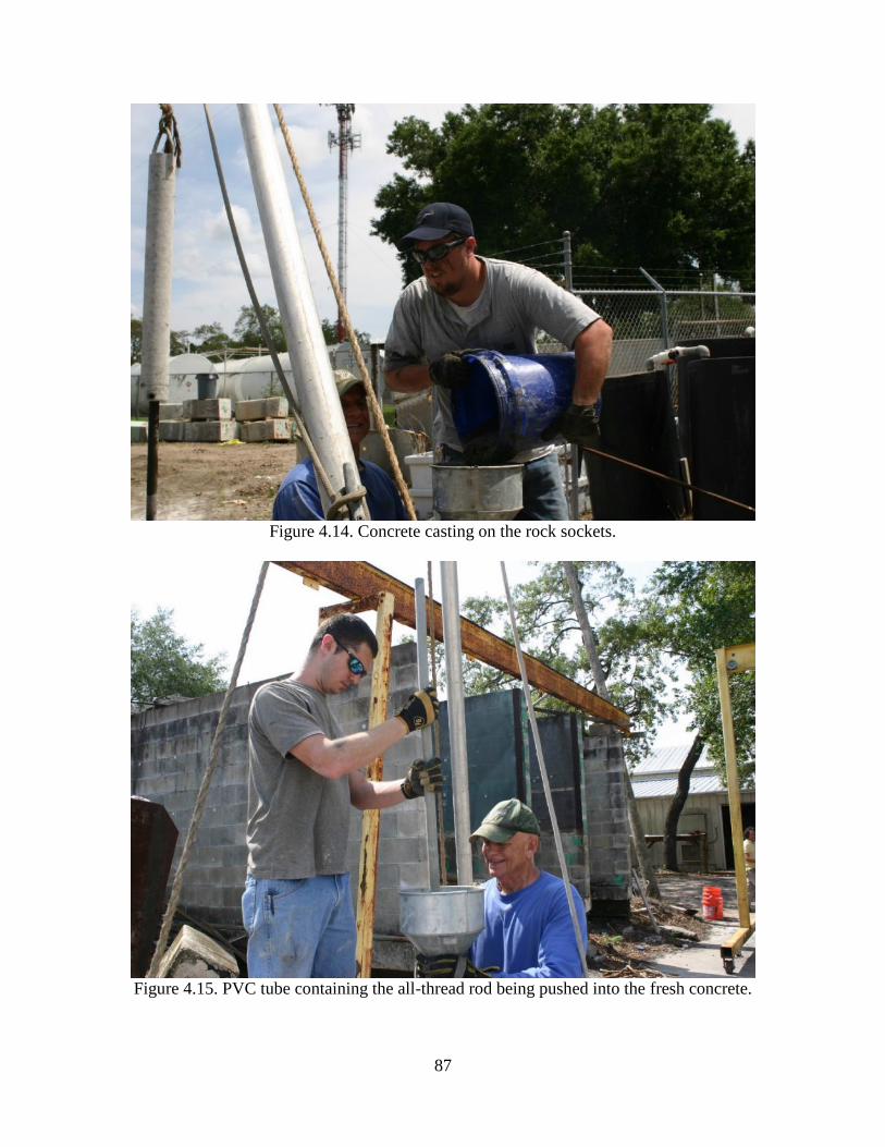
87

Figure 4.14. Concrete casting on the rock sockets.

Figure 4.15. PVC tube containing the all-thread rod being pushed into the fresh concrete.

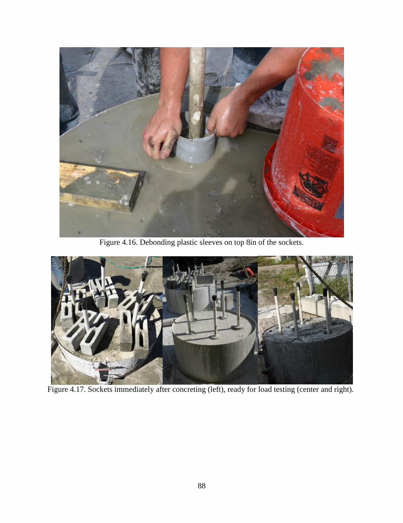
88

Figure 4.16. Debonding plastic sleeves on top 8in of the sockets.

Figure 4.17. Sockets immediately after concreting (left), ready for load testing (center and right).

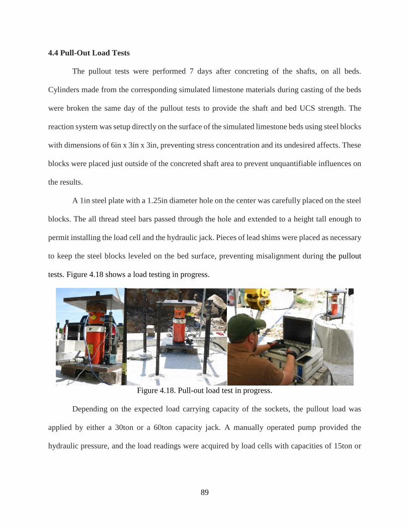
89

4.4 Pull-Out Load Tests

The pullout tests were performed 7 days after concreting of the shafts, on all beds.

Cylinders made from the corresponding simulated limestone materials during casting of the beds

were broken the same day of the pullout tests to provide the shaft and bed UCS strength. The

reaction system was setup directly on the surface of the simulated limestone beds using steel blocks

with dimensions of 6in x 3in x 3in, preventing stress concentration and its undesired affects. These

blocks were placed just outside of the concreted shaft area to prevent unquantifiable influences on

the results.

A 1in steel plate with a 1.25in diameter hole on the center was carefully placed on the steel

blocks. The all thread steel bars passed through the hole and extended to a height tall enough to

permit installing the load cell and the hydraulic jack. Pieces of lead shims were placed as necessary

to keep the steel blocks leveled on the bed surface, preventing misalignment during the pullout

tests. Figure 4.18 shows a load testing in progress.

Figure 4.18. Pull-out load test in progress.

Depending on the expected load carrying capacity of the sockets, the pullout load was

applied by either a 30ton or a 60ton capacity jack. A manually operated pump provided the

hydraulic pressure, and the load readings were acquired by load cells with capacities of 15ton or

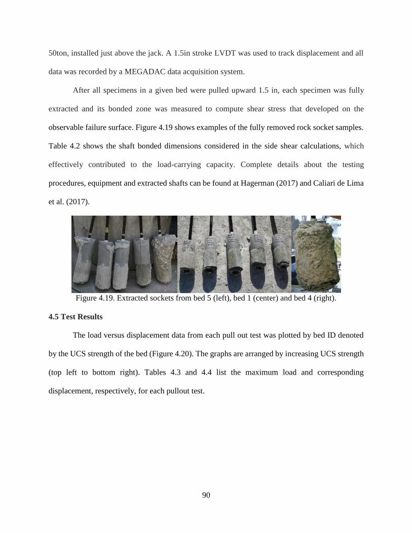
90

50ton, installed just above the jack. A 1.5in stroke LVDT was used to track displacement and all

data was recorded by a MEGADAC data acquisition system.

After all specimens in a given bed were pulled upward 1.5 in, each specimen was fully

extracted and its bonded zone was measured to compute shear stress that developed on the

observable failure surface. Figure 4.19 shows examples of the fully removed rock socket samples.

Table 4.2 shows the shaft bonded dimensions considered in the side shear calculations, which

effectively contributed to the load-carrying capacity. Complete details about the testing

procedures, equipment and extracted shafts can be found at Hagerman (2017) and Caliari de Lima

et al. (2017).

Figure 4.19. Extracted sockets from bed 5 (left), bed 1 (center) and bed 4 (right).

4.5 Test Results

The load versus displacement data from each pull out test was plotted by bed ID denoted

by the UCS strength of the bed (Figure 4.20). The graphs are arranged by increasing UCS strength

(top left to bottom right). Tables 4.3 and 4.4 list the maximum load and corresponding

displacement, respectively, for each pullout test.

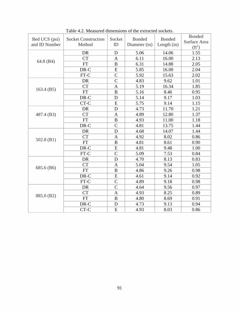
91

Table 4.2. Measured dimensions of the extracted sockets.

Bed UCS (psi)and ID Number

Socket ConstructionMethod

SocketID

BondedDiameter (in)

BondedLength (in)

BondedSurface Area

(ft2)

64.8 (B4)

DR D 5.06 14.06 1.55CT A 6.11 16.00 2.13FT B 6.31 14.88 2.05

DR-C E 5.85 16.00 2.04FT-C C 5.92 15.63 2.02

163.4 (B5)

DR C 4.83 9.62 1.01CT A 5.19 16.34 1.85FT B 5.16 8.46 0.95

DR-C D 5.14 9.17 1.03CT-C E 5.75 9.14 1.15

487.4 (B3)DR D 4.73 11.70 1.21CT A 4.89 12.80 1.37FT B 4.93 11.00 1.18

DR-C C 4.81 13.75 1.44

502.8 (B1)

DR D 4.68 14.07 1.44CT A 4.92 8.02 0.86FT B 4.81 8.61 0.90

DR-C E 4.81 9.48 1.00FT-C C 5.09 7.53 0.84

685.6 (B6)

DR D 4.70 8.13 0.83CT A 5.04 9.54 1.05FT B 4.86 9.26 0.98

DR-C E 4.61 9.14 0.92FT-C C 4.89 9.18 0.98

885.0 (B2)

DR C 4.64 9.56 0.97CT A 4.93 8.25 0.89FT B 4.80 8.69 0.91

DR-C D 4.73 9.13 0.94CT-C E 4.93 8.03 0.86

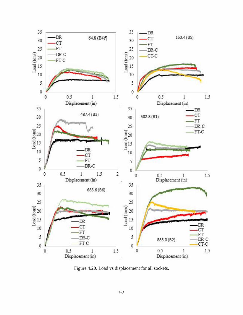
92

Figure 4.20. Load vs displacement for all sockets.

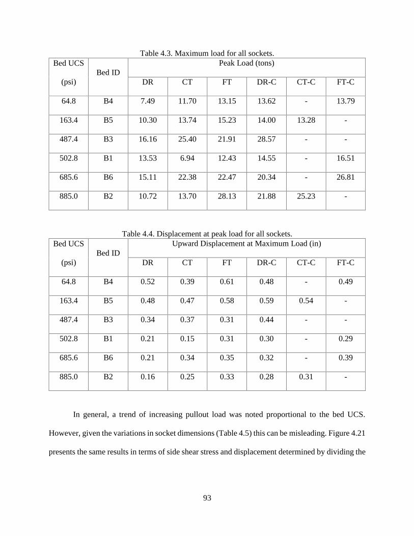
93

Table 4.3. Maximum load for all sockets.Bed UCS

(psi)Bed ID

Peak Load (tons)

DR CT FT DR-C CT-C FT-C

64.8 B4 7.49 11.70 13.15 13.62 - 13.79

163.4 B5 10.30 13.74 15.23 14.00 13.28 -

487.4 B3 16.16 25.40 21.91 28.57 - -

502.8 B1 13.53 6.94 12.43 14.55 - 16.51

685.6 B6 15.11 22.38 22.47 20.34 - 26.81

885.0 B2 10.72 13.70 28.13 21.88 25.23 -

Table 4.4. Displacement at peak load for all sockets.Bed UCS

(psi)Bed ID

Upward Displacement at Maximum Load (in)

DR CT FT DR-C CT-C FT-C

64.8 B4 0.52 0.39 0.61 0.48 - 0.49

163.4 B5 0.48 0.47 0.58 0.59 0.54 -

487.4 B3 0.34 0.37 0.31 0.44 - -

502.8 B1 0.21 0.15 0.31 0.30 - 0.29

685.6 B6 0.21 0.34 0.35 0.32 - 0.39

885.0 B2 0.16 0.25 0.33 0.28 0.31 -

In general, a trend of increasing pullout load was noted proportional to the bed UCS.

However, given the variations in socket dimensions (Table 4.5) this can be misleading. Figure 4.21

presents the same results in terms of side shear stress and displacement determined by dividing the

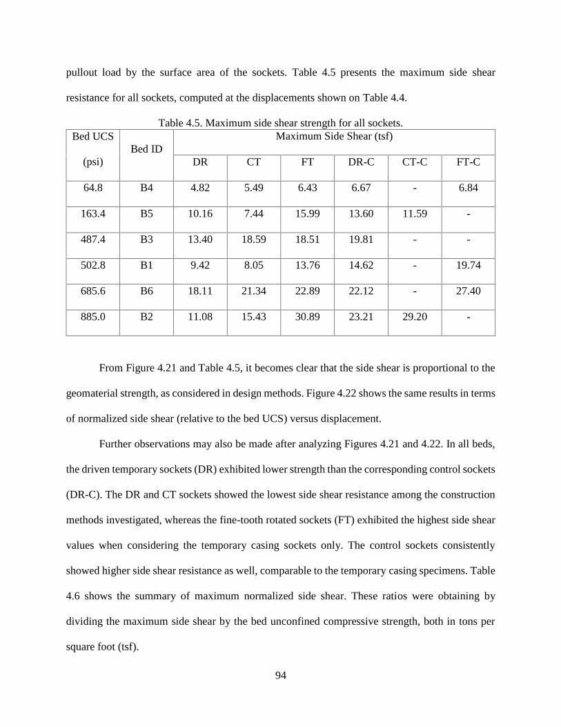
94

pullout load by the surface area of the sockets. Table 4.5 presents the maximum side shear

resistance for all sockets, computed at the displacements shown on Table 4.4.

Table 4.5. Maximum side shear strength for all sockets.Bed UCS

(psi)Bed ID

Maximum Side Shear (tsf)

DR CT FT DR-C CT-C FT-C

64.8 B4 4.82 5.49 6.43 6.67 - 6.84

163.4 B5 10.16 7.44 15.99 13.60 11.59 -

487.4 B3 13.40 18.59 18.51 19.81 - -

502.8 B1 9.42 8.05 13.76 14.62 - 19.74

685.6 B6 18.11 21.34 22.89 22.12 - 27.40

885.0 B2 11.08 15.43 30.89 23.21 29.20 -

From Figure 4.21 and Table 4.5, it becomes clear that the side shear is proportional to the

geomaterial strength, as considered in design methods. Figure 4.22 shows the same results in terms

of normalized side shear (relative to the bed UCS) versus displacement.

Further observations may also be made after analyzing Figures 4.21 and 4.22. In all beds,

the driven temporary sockets (DR) exhibited lower strength than the corresponding control sockets

(DR-C). The DR and CT sockets showed the lowest side shear resistance among the construction

methods investigated, whereas the fine-tooth rotated sockets (FT) exhibited the highest side shear

values when considering the temporary casing sockets only. The control sockets consistently

showed higher side shear resistance as well, comparable to the temporary casing specimens. Table

4.6 shows the summary of maximum normalized side shear. These ratios were obtaining by

dividing the maximum side shear by the bed unconfined compressive strength, both in tons per

square foot (tsf).

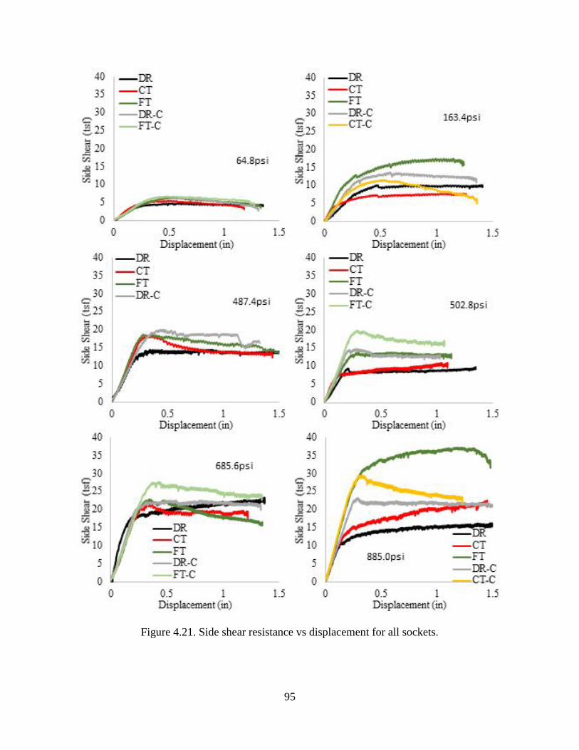
95

Figure 4.21. Side shear resistance vs displacement for all sockets.

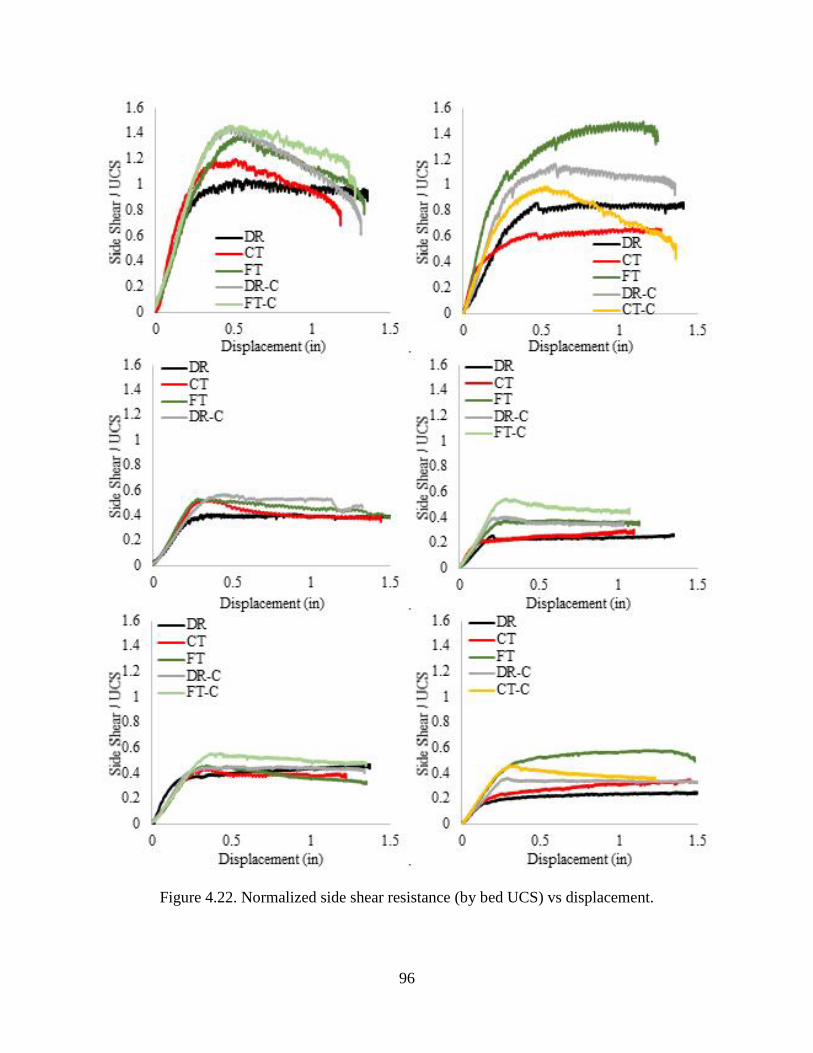
96

Figure 4.22. Normalized side shear resistance (by bed UCS) vs displacement.

97

Table 4.6. Maximum normalized side shear.Bed UCS

(psi)Bed ID

Maximum Normalized Side Shear (Side Shear / UCS Ratio)DR CT FT DR-C CT-C FT-C

64.8 B4 1.03 1.18 1.38 1.43 - 1.47163.4 B5 0.86 0.63 1.36 1.16 0.99 -487.4 B3 0.38 0.53 0.53 0.56 - -502.8 B1 0.26 0.22 0.38 0.40 - 0.55685.6 B6 0.37 0.43 0.46 0.45 - 0.56885.0 B2 0.17 0.24 0.48 0.36 0.46 -

Table 4.7 shows the ultimate side shear ratios between the temporary casing and the control

sockets, using the values shown on Table 4.4. Figure 4.23 shows the side shear ratios versus

displacement.

Table 4.7. Side shear ratios between temporary and respective control casings.

Casing TypeBed UCS (psi)

and IDPeak Displacement

(in)Ultimate

Stress Ratio

Average Peak

Stress Ratio

Driven (DR)

64.8 (B4) 0.52 0.72

0.68163.4 (B5) 0.48 0.75487.4 (B3) 0.34 0.68502.8 (B1) 0.21 0.64685.6 (B6) 0.21 0.82885.0 (B2) 0.16 0.48

Coarse-ToothRotated (CT)

163.4 (B5) 0.47 0.64 0.59885.0 (B2) 0.25 0.53

Fine-ToothRotated (FT)

64.8 (B4) 0.61 0.940.82

502.8 (B1) 0.31 0.70685.6 (B6) 0.35 0.84

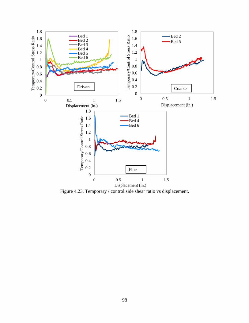
98

Figure 4.23. Temporary / control side shear ratio vs displacement.

0

0.2

0.4

0.6

0.8

1

1.2

1.4

1.6

1.8

0 0.5 1 1.5

Tem

pora

ry/C

ontr

ol S

tres

s R

atio

Displacement (in.)

Bed 1Bed 2Bed 3Bed 4Bed 5Bed 6

Driven

0

0.2

0.4

0.6

0.8

1

1.2

1.4

1.6

1.8

0 0.5 1 1.5

Tem

pora

ry/C

ontr

ol S

tres

s R

atio

Displacement (in.)

Bed 2Bed 5

Coarse

0

0.2

0.4

0.6

0.8

1

1.2

1.4

1.6

1.8

0 0.5 1 1.5

Tem

pora

ry/C

ontr

ol S

tres

s R

atio

Displacement (in.)

Bed 1Bed 4Bed 6

Fine

99

CHAPTER 5: DISCUSSIONS AND CONCLUSION

5.1 Overview

Present design methods for side shear resistance of drilled shafts in soils and rock were

derived and/or verified from full scale case studies, but do not make any distinctions for a wide

range of construction techniques. Instead, the design parameters encompass all excavation

procedures, and therefore the resulting calculated side shear is solely dependent on the soil type

regardless of whether slurry, temporary casing or dry construction is used.

This research program separately investigated the effects of slurry and casing stabilization

of drilled shaft excavations. For slurry excavations, the type of slurry (e.g. mineral or polymer)

and open excavation / slurry exposure time was altered to identify how sandy soils might be

affected (Chapter 3). Clayey soils were not addressed as very little slurry inflow occurs into clay

and slurry stabilization is often not needed. Similarly, the effects of different procedures to install

and extract temporary casings in simulated limestone were examined (Chapter 4).

This Chapter presents further discussions regarding the results, which evidence even more

that there are significant differences in side shear due to the different excavation stabilization

methods.

5.2 Slurry Constructed Shafts

Thirty two small scale drilled shafts were constructed and pull-out tested for quantifying

the effects of 4 different commercial drilling slurry products used in the field (one bentonite and

three polymers). The shafts were, nominally, 4in diameter and 7ft to 8ft long.

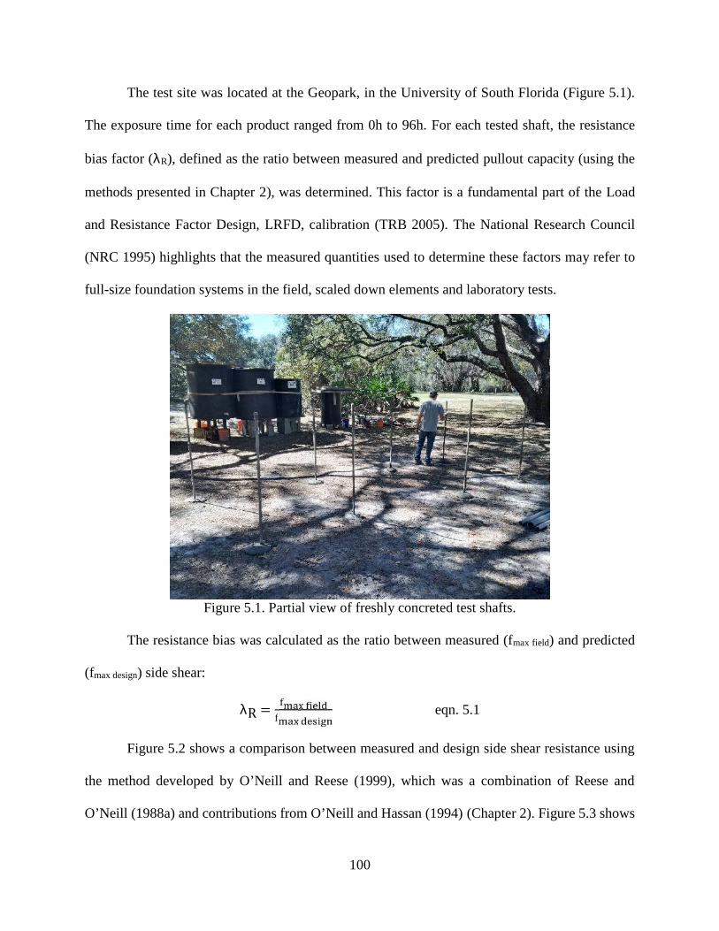
100

The test site was located at the Geopark, in the University of South Florida (Figure 5.1).

The exposure time for each product ranged from 0h to 96h. For each tested shaft, the resistance

bias factor (R), defined as the ratio between measured and predicted pullout capacity (using the

methods presented in Chapter 2), was determined. This factor is a fundamental part of the Load

and Resistance Factor Design, LRFD, calibration (TRB 2005). The National Research Council

(NRC 1995) highlights that the measured quantities used to determine these factors may refer to

full-size foundation systems in the field, scaled down elements and laboratory tests.

Figure 5.1. Partial view of freshly concreted test shafts.

The resistance bias was calculated as the ratio between measured (fmax field) and predicted

(fmax design) side shear:

R = eqn. 5.1

Figure 5.2 shows a comparison between measured and design side shear resistance using

the method developed by O’Neill and Reese (1999), which was a combination of Reese and

O’Neill (1988a) and contributions from O’Neill and Hassan (1994) (Chapter 2). Figure 5.3 shows

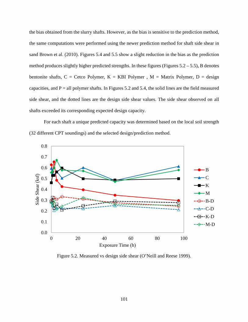
101

the bias obtained from the slurry shafts. However, as the bias is sensitive to the prediction method,

the same computations were performed using the newer prediction method for shaft side shear in

sand Brown et al. (2010). Figures 5.4 and 5.5 show a slight reduction in the bias as the prediction

method produces slightly higher predicted strengths. In these figures (Figures 5.2 – 5.5), B denotes

bentonite shafts, C = Cetco Polymer, K = KBI Polymer , M = Matrix Polymer, D = design

capacities, and P = all polymer shafts. In Figures 5.2 and 5.4, the solid lines are the field measured

side shear, and the dotted lines are the design side shear values. The side shear observed on all

shafts exceeded its corresponding expected design capacity.

For each shaft a unique predicted capacity was determined based on the local soil strength

(32 different CPT soundings) and the selected design/prediction method.

Figure 5.2. Measured vs design side shear (O’Neill and Reese 1999).

0.0

0.1

0.2

0.3

0.4

0.5

0.6

0.7

0.8

0 20 40 60 80 100

Sid

e S

hear

(ks

f)

Exposure Time (h)

B

C

K

M

B-D

C-D

K-D

M-D

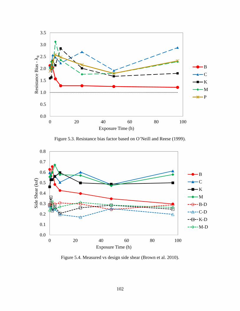
102

Figure 5.3. Resistance bias factor based on O’Neill and Reese (1999).

Figure 5.4. Measured vs design side shear (Brown et al. 2010).

0.0

0.5

1.0

1.5

2.0

2.5

3.0

3.5

0 20 40 60 80 100

Res

ista

nce

Bia

s-

R

Exposure Time (h)

B

C

K

M

P

0.0

0.1

0.2

0.3

0.4

0.5

0.6

0.7

0.8

0 20 40 60 80 100

Sid

e S

hear

(ks

f)

Exposure Time (h)

B

C

K

M

B-D

C-D

K-D

M-D

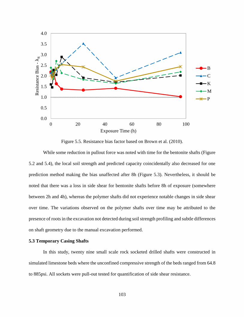
103

Figure 5.5. Resistance bias factor based on Brown et al. (2010).

While some reduction in pullout force was noted with time for the bentonite shafts (Figure

5.2 and 5.4), the local soil strength and predicted capacity coincidentally also decreased for one

prediction method making the bias unaffected after 8h (Figure 5.3). Nevertheless, it should be

noted that there was a loss in side shear for bentonite shafts before 8h of exposure (somewhere

between 2h and 4h), whereas the polymer shafts did not experience notable changes in side shear

over time. The variations observed on the polymer shafts over time may be attributed to the

presence of roots in the excavation not detected during soil strength profiling and subtle differences

on shaft geometry due to the manual excavation performed.

5.3 Temporary Casing Shafts

In this study, twenty nine small scale rock socketed drilled shafts were constructed in

simulated limestone beds where the unconfined compressive strength of the beds ranged from 64.8

to 885psi. All sockets were pull-out tested for quantification of side shear resistance.

0.0

0.5

1.0

1.5

2.0

2.5

3.0

3.5

4.0

0 20 40 60 80 100

Res

ista

nce

Bia

s-

R

Exposure Time (h)

B

C

K

M

P

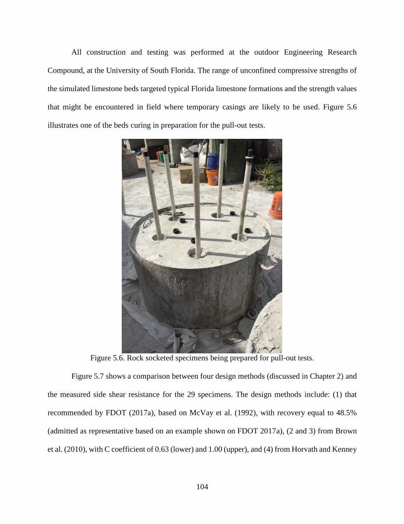
104

All construction and testing was performed at the outdoor Engineering Research

Compound, at the University of South Florida. The range of unconfined compressive strengths of

the simulated limestone beds targeted typical Florida limestone formations and the strength values

that might be encountered in field where temporary casings are likely to be used. Figure 5.6

illustrates one of the beds curing in preparation for the pull-out tests.

Figure 5.6. Rock socketed specimens being prepared for pull-out tests.

Figure 5.7 shows a comparison between four design methods (discussed in Chapter 2) and

the measured side shear resistance for the 29 specimens. The design methods include: (1) that

recommended by FDOT (2017a), based on McVay et al. (1992), with recovery equal to 48.5%

(admitted as representative based on an example shown on FDOT 2017a), (2 and 3) from Brown

et al. (2010), with C coefficient of 0.63 (lower) and 1.00 (upper), and (4) from Horvath and Kenney

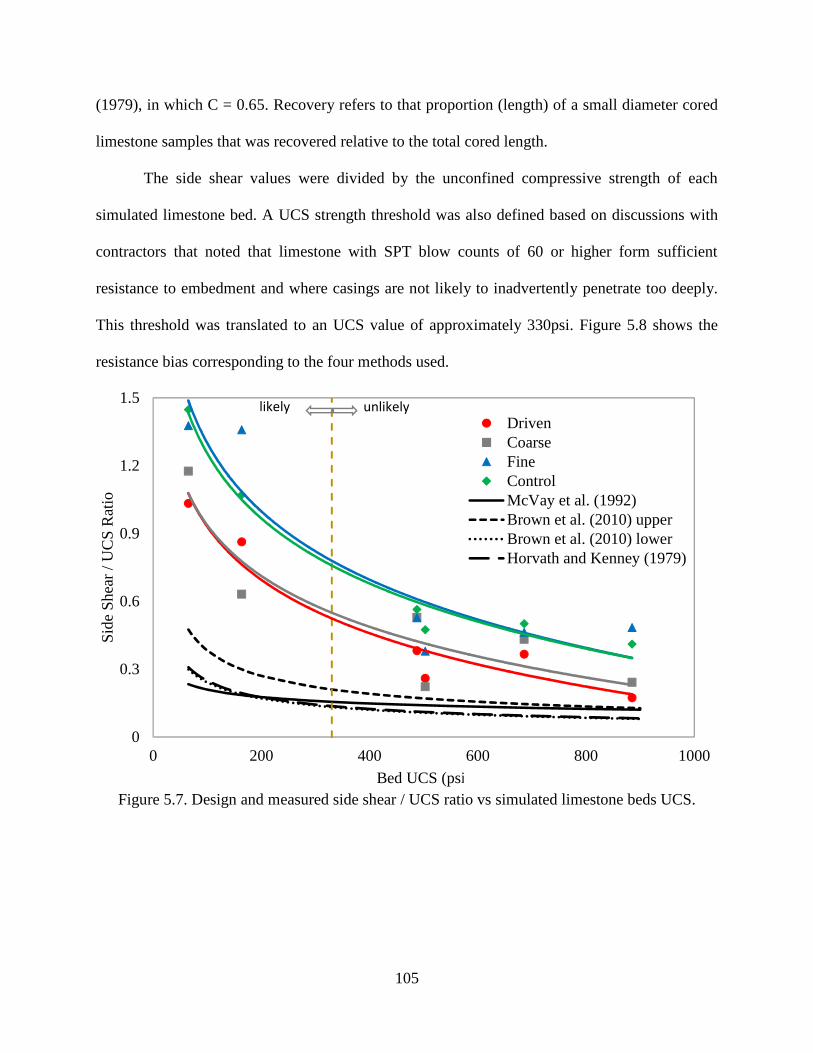
105

(1979), in which C = 0.65. Recovery refers to that proportion (length) of a small diameter cored

limestone samples that was recovered relative to the total cored length.

The side shear values were divided by the unconfined compressive strength of each

simulated limestone bed. A UCS strength threshold was also defined based on discussions with

contractors that noted that limestone with SPT blow counts of 60 or higher form sufficient

resistance to embedment and where casings are not likely to inadvertently penetrate too deeply.

This threshold was translated to an UCS value of approximately 330psi. Figure 5.8 shows the

resistance bias corresponding to the four methods used.

Figure 5.7. Design and measured side shear / UCS ratio vs simulated limestone beds UCS.

0

0.3

0.6

0.9

1.2

1.5

0 200 400 600 800 1000

Sid

e S

hear

/ U

CS

Rat

io

Bed UCS (psi)

DrivenCoarseFineControlMcVay et al. (1992)Brown et al. (2010) upperBrown et al. (2010) lowerHorvath and Kenney (1979)

unlikelylikely

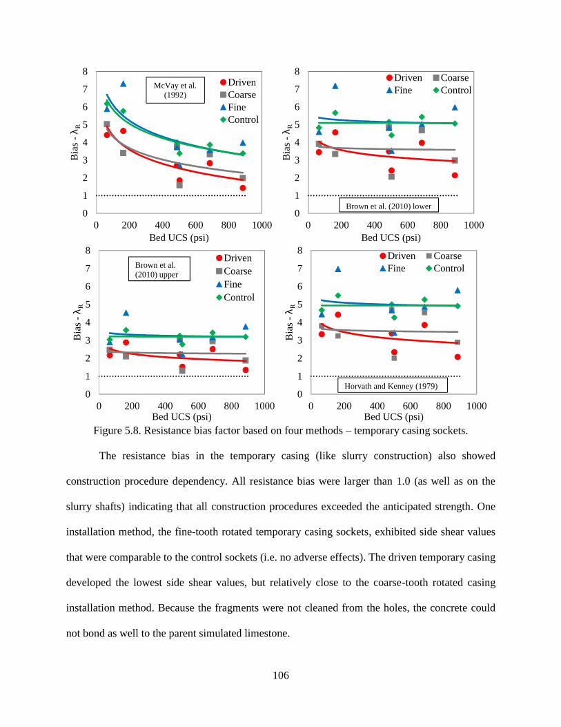
106

Figure 5.8. Resistance bias factor based on four methods – temporary casing sockets.

The resistance bias in the temporary casing (like slurry construction) also showed

construction procedure dependency. All resistance bias were larger than 1.0 (as well as on the

slurry shafts) indicating that all construction procedures exceeded the anticipated strength. One

installation method, the fine-tooth rotated temporary casing sockets, exhibited side shear values

that were comparable to the control sockets (i.e. no adverse effects). The driven temporary casing

developed the lowest side shear values, but relatively close to the coarse-tooth rotated casing

installation method. Because the fragments were not cleaned from the holes, the concrete could

not bond as well to the parent simulated limestone.

0

1

2

3

4

5

6

7

8

0 200 400 600 800 1000

Bia

s-

R

Bed UCS (psi)

DrivenCoarseFineControl

McVay et al.(1992)

0

1

2

3

4

5

6

7

8

0 200 400 600 800 1000

Bia

s-

R

Bed UCS (psi)

Driven CoarseFine Control

Brown et al. (2010) lower

0

1

2

3

4

5

6

7

8

0 200 400 600 800 1000

Bia

s-

R

Bed UCS (psi)

DrivenCoarseFineControl

Brown et al.(2010) upper

0

1

2

3

4

5

6

7

8

0 200 400 600 800 1000

Bia

s-

R

Bed UCS (psi)

Driven CoarseFine Control

Horvath and Kenney (1979)

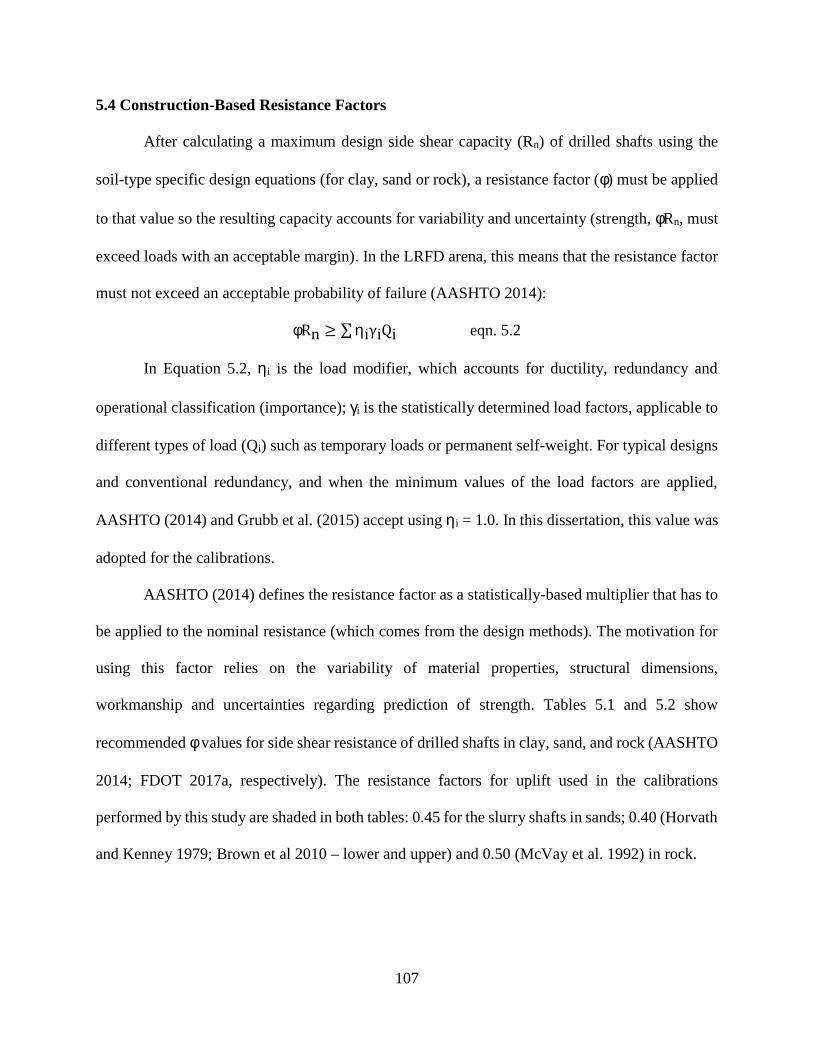
107

5.4 Construction-Based Resistance Factors

After calculating a maximum design side shear capacity (Rn) of drilled shafts using the

soil-type specific design equations (for clay, sand or rock), a resistance factor () must be applied

to that value so the resulting capacity accounts for variability and uncertainty (strength, Rn, must

exceed loads with an acceptable margin). In the LRFD arena, this means that the resistance factor

must not exceed an acceptable probability of failure (AASHTO 2014):

Rn ≥ ∑iγiQi eqn. 5.2

In Equation 5.2, i is the load modifier, which accounts for ductility, redundancy and

operational classification (importance); i is the statistically determined load factors, applicable to

different types of load (Qi) such as temporary loads or permanent self-weight. For typical designs

and conventional redundancy, and when the minimum values of the load factors are applied,

AASHTO (2014) and Grubb et al. (2015) accept using i = 1.0. In this dissertation, this value was

adopted for the calibrations.

AASHTO (2014) defines the resistance factor as a statistically-based multiplier that has to

be applied to the nominal resistance (which comes from the design methods). The motivation for

using this factor relies on the variability of material properties, structural dimensions,

workmanship and uncertainties regarding prediction of strength. Tables 5.1 and 5.2 show

recommended values for side shear resistance of drilled shafts in clay, sand, and rock (AASHTO

2014; FDOT 2017a, respectively). The resistance factors for uplift used in the calibrations

performed by this study are shaded in both tables: 0.45 for the slurry shafts in sands; 0.40 (Horvath

and Kenney 1979; Brown et al 2010 – lower and upper) and 0.50 (McVay et al. 1992) in rock.

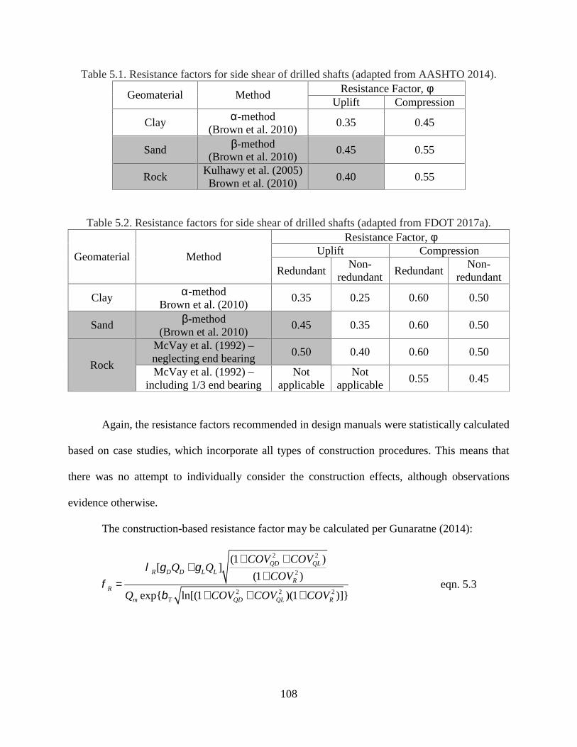
108

Table 5.1. Resistance factors for side shear of drilled shafts (adapted from AASHTO 2014).

Geomaterial Method Resistance Factor, Uplift Compression

Clay -method(Brown et al. 2010)

0.35 0.45

Sand -method(Brown et al. 2010)

0.45 0.55

RockKulhawy et al. (2005)Brown et al. (2010)

0.40 0.55

Table 5.2. Resistance factors for side shear of drilled shafts (adapted from FDOT 2017a).

Geomaterial Method

Resistance Factor, Uplift Compression

RedundantNon-

redundantRedundant

Non-redundant

Clay -methodBrown et al. (2010)

0.35 0.25 0.60 0.50

Sand -method(Brown et al. 2010)

0.45 0.35 0.60 0.50

Rock

McVay et al. (1992) –neglecting end bearing

0.50 0.40 0.60 0.50

McVay et al. (1992) –including 1/3 end bearing

Notapplicable

Notapplicable

0.55 0.45

Again, the resistance factors recommended in design manuals were statistically calculated

based on case studies, which incorporate all types of construction procedures. This means that

there was no attempt to individually consider the construction effects, although observations

evidence otherwise.

The construction-based resistance factor may be calculated per Gunaratne (2014):

2 2

2

2 2 2

(1 )[ ]

(1 )

exp{ ln[(1 )(1 )]}

QD QLR D D L L

RR

m T QD QL R

COV COVQ Q

COV

Q COV COV COV

eqn. 5.3

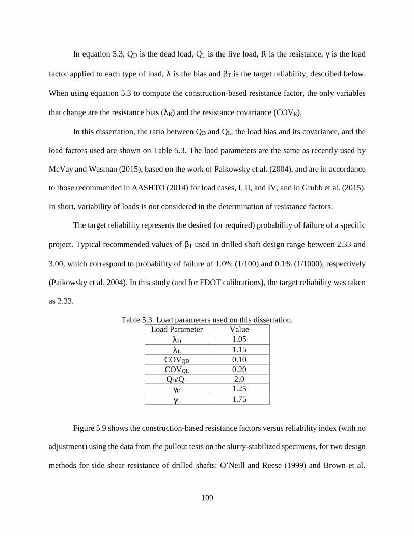
109

In equation 5.3, QD is the dead load, QL is the live load, R is the resistance, is the load

factor applied to each type of load, is the bias and T is the target reliability, described below.

When using equation 5.3 to compute the construction-based resistance factor, the only variables

that change are the resistance bias (R) and the resistance covariance (COVR).

In this dissertation, the ratio between QD and QL, the load bias and its covariance, and the

load factors used are shown on Table 5.3. The load parameters are the same as recently used by

McVay and Wasman (2015), based on the work of Paikowsky et al. (2004), and are in accordance

to those recommended in AASHTO (2014) for load cases, I, II, and IV, and in Grubb et al. (2015).

In short, variability of loads is not considered in the determination of resistance factors.

The target reliability represents the desired (or required) probability of failure of a specific

project. Typical recommended values of T used in drilled shaft design range between 2.33 and

3.00, which correspond to probability of failure of 1.0% (1/100) and 0.1% (1/1000), respectively

(Paikowsky et al. 2004). In this study (and for FDOT calibrations), the target reliability was taken

as 2.33.

Table 5.3. Load parameters used on this dissertation.Load Parameter Value

D 1.05L 1.15

COVQD 0.10COVQL 0.20QD/QL 2.0

D 1.25L 1.75

Figure 5.9 shows the construction-based resistance factors versus reliability index (with no

adjustment) using the data from the pullout tests on the slurry-stabilized specimens, for two design

methods for side shear resistance of drilled shafts: O’Neill and Reese (1999) and Brown et al.

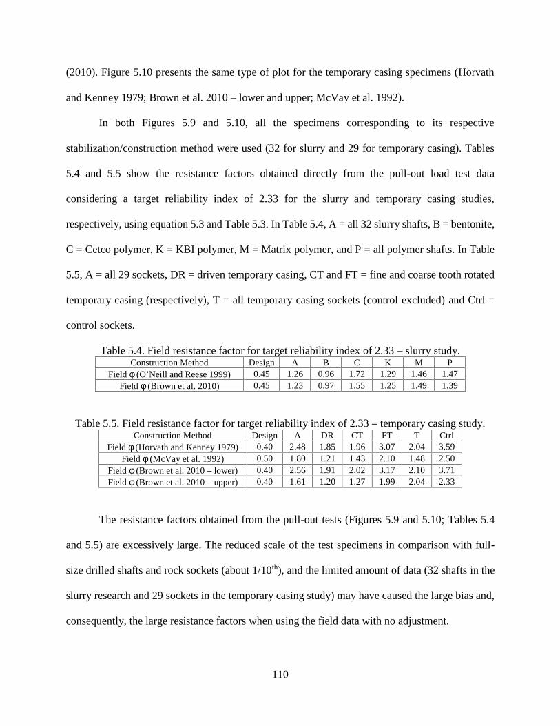
110

(2010). Figure 5.10 presents the same type of plot for the temporary casing specimens (Horvath

and Kenney 1979; Brown et al. 2010 – lower and upper; McVay et al. 1992).

In both Figures 5.9 and 5.10, all the specimens corresponding to its respective

stabilization/construction method were used (32 for slurry and 29 for temporary casing). Tables

5.4 and 5.5 show the resistance factors obtained directly from the pull-out load test data

considering a target reliability index of 2.33 for the slurry and temporary casing studies,

respectively, using equation 5.3 and Table 5.3. In Table 5.4, A = all 32 slurry shafts, B = bentonite,

C = Cetco polymer, K = KBI polymer, M = Matrix polymer, and P = all polymer shafts. In Table

5.5, A = all 29 sockets, DR = driven temporary casing, CT and FT = fine and coarse tooth rotated

temporary casing (respectively), T = all temporary casing sockets (control excluded) and Ctrl =

control sockets.

Table 5.4. Field resistance factor for target reliability index of 2.33 – slurry study.Construction Method Design A B C K M P

Field (O’Neill and Reese 1999) 0.45 1.26 0.96 1.72 1.29 1.46 1.47Field (Brown et al. 2010) 0.45 1.23 0.97 1.55 1.25 1.49 1.39

Table 5.5. Field resistance factor for target reliability index of 2.33 – temporary casing study.Construction Method Design A DR CT FT T Ctrl

Field (Horvath and Kenney 1979) 0.40 2.48 1.85 1.96 3.07 2.04 3.59Field (McVay et al. 1992) 0.50 1.80 1.21 1.43 2.10 1.48 2.50

Field (Brown et al. 2010 – lower) 0.40 2.56 1.91 2.02 3.17 2.10 3.71Field (Brown et al. 2010 – upper) 0.40 1.61 1.20 1.27 1.99 2.04 2.33

The resistance factors obtained from the pull-out tests (Figures 5.9 and 5.10; Tables 5.4

and 5.5) are excessively large. The reduced scale of the test specimens in comparison with full-

size drilled shafts and rock sockets (about 1/10th), and the limited amount of data (32 shafts in the

slurry research and 29 sockets in the temporary casing study) may have caused the large bias and,

consequently, the large resistance factors when using the field data with no adjustment.

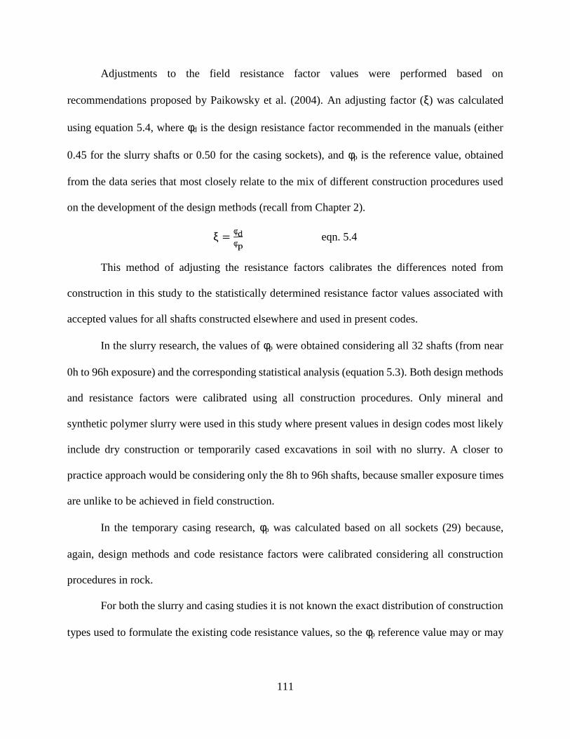
111

Adjustments to the field resistance factor values were performed based on

recommendations proposed by Paikowsky et al. (2004). An adjusting factor () was calculated

using equation 5.4, where d is the design resistance factor recommended in the manuals (either

0.45 for the slurry shafts or 0.50 for the casing sockets), and p is the reference value, obtained

from the data series that most closely relate to the mix of different construction procedures used

on the development of the design methods (recall from Chapter 2).

=

eqn. 5.4

This method of adjusting the resistance factors calibrates the differences noted from

construction in this study to the statistically determined resistance factor values associated with

accepted values for all shafts constructed elsewhere and used in present codes.

In the slurry research, the values of p were obtained considering all 32 shafts (from near

0h to 96h exposure) and the corresponding statistical analysis (equation 5.3). Both design methods

and resistance factors were calibrated using all construction procedures. Only mineral and

synthetic polymer slurry were used in this study where present values in design codes most likely

include dry construction or temporarily cased excavations in soil with no slurry. A closer to

practice approach would be considering only the 8h to 96h shafts, because smaller exposure times

are unlike to be achieved in field construction.

In the temporary casing research, p was calculated based on all sockets (29) because,

again, design methods and code resistance factors were calibrated considering all construction

procedures in rock.

For both the slurry and casing studies it is not known the exact distribution of construction

types used to formulate the existing code resistance values, so the p reference value may or may

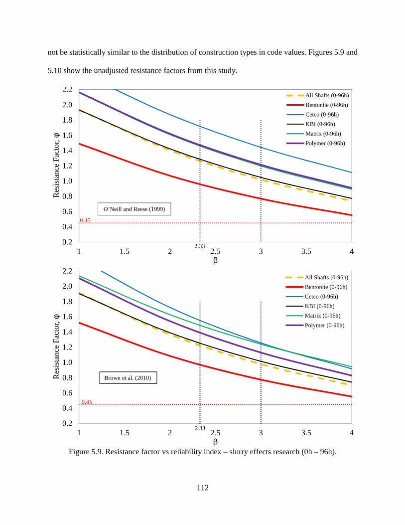
112

not be statistically similar to the distribution of construction types in code values. Figures 5.9 and

5.10 show the unadjusted resistance factors from this study.

Figure 5.9. Resistance factor vs reliability index – slurry effects research (0h – 96h).

0.2

0.4

0.6

0.8

1.0

1.2

1.4

1.6

1.8

2.0

2.2

1 1.5 2 2.5 3 3.5 4

Res

ista

nce

Fact

or,

All Shafts (0-96h)

Bentonite (0-96h)

Cetco (0-96h)

KBI (0-96h)

Matrix (0-96h)

Polymer (0-96h)

2.33

0.45

0.2

0.4

0.6

0.8

1.0

1.2

1.4

1.6

1.8

2.0

2.2

1 1.5 2 2.5 3 3.5 4

Res

ista

nce

Fact

or,

All Shafts (0-96h)

Bentonite (0-96h)

Cetco (0-96h)

KBI (0-96h)

Matrix (0-96h)

Polymer (0-96h)

2.33

0.45

Brown et al. (2010)

O’Neill and Reese (1999)

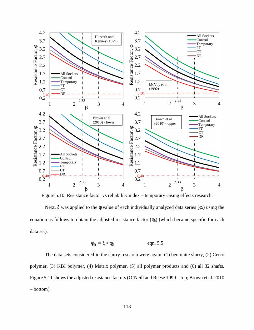
113

Figure 5.10. Resistance factor vs reliability index – temporary casing effects research.

Next, was applied to the value of each individually analyzed data series (s) using the

equation as follows to obtain the adjusted resistance factor (a) (which became specific for each

data set).

a = ∗ s eqn. 5.5

The data sets considered in the slurry research were again: (1) bentonite slurry, (2) Cetco

polymer, (3) KBI polymer, (4) Matrix polymer, (5) all polymer products and (6) all 32 shafts.

Figure 5.11 shows the adjusted resistance factors (O’Neill and Reese 1999 – top; Brown et al. 2010

– bottom).

0.2

0.7

1.2

1.7

2.2

2.7

3.2

3.7

4.2

1 2 3 4

Res

ista

nce

Fact

or,

All SocketsControlTemporaryFTCTDR

2.33

0.400.2

0.7

1.2

1.7

2.2

2.7

3.2

3.7

4.2

1 2 3 4

Res

ista

nce

Fact

or,

All SocketsControlTemporaryFTCTDR

2.33

0.50

0.2

0.7

1.2

1.7

2.2

2.7

3.2

3.7

4.2

1 2 3 4

Res

ista

nce

Fact

or,

All SocketsControlTemporaryFTCTDR

2.33

0.400.2

0.7

1.2

1.7

2.2

2.7

3.2

3.7

4.2

1 2 3 4

Res

ista

nce

Fact

or,

All SocketsControlTemporaryFTCTDR

2.33

0.40

Brown et al.(2010) - upper

McVay et al.(1992)

Horvath andKenney (1979)

Brown et al.(2010) - lower

114

In the temporary casing research, the individually analyzed data sets were again: (1) driven

temporary casing (DR), (2) coarse-tooth rotated temporary casing (CT), (3) fine-tooth rotated

temporary casing (FT), (4) all temporary casing sockets, (5) all control specimens and (6) all 29

sockets. Figure 5.12 shows the adjusted resistance factors based on the design methods proposed

by Horvath and Kenney (1979), Brown et al. (2010) – lower and upper (plot on top), and McVay

et al. (1992) (plot on bottom). As expected, the adjusted resistance factors for the first three cited

methods resulted in the same effect as these methods all use the same equation for computing the

design side shear only changing “C”.

Tables 5.6 and 5.7 show the adjusted resistance factors considering a target reliability index

of 2.33, for the slurry and temporary casing studies, respectively.

Table 5.6. Adjusted resistance factor for target reliability index of 2.33 – slurry study.Construction Method Design All B C K M P

Adjusted (O’Neill and Reese 1999) 0.45 0.45 0.34 0.61 0.46 0.52 0.52Adjusted (Brown et al. 2010) 0.45 0.45 0.35 0.57 0.46 0.54 0.51

Table 5.7. Adjusted resistance factor for target reliability index of 2.33 – temporary casing study.Construction Method Design All DR CT FT T Ctrl

Adjusted (Horvath and Kenney 1979) 0.40 0.40 0.30 0.31 0.49 0.33 0.58Adjusted (McVay et al. 1992) 0.50 0.50 0.33 0.40 0.58 0.41 0.69Adjusted (Brown et al. 2010 – lower) 0.40 0.40 0.30 0.31 0.49 0.33 0.58Adjusted (Brown et al. 2010 – upper) 0.40 0.40 0.30 0.31 0.49 0.33 0.58

From the presented results, it is again evident that different construction methods may

result in significantly varying adjusted resistance factors (this statement is also observable in the

non-adjusted resistance factors). The resistance factor variations observed between design methods

was less significant and relatively small.

115

Figure 5.11. Adjusted resistance factors – slurry study.

0.2

0.4

0.6

0.8

1.0

1 1.5 2 2.5 3 3.5 4

Adj

uste

d R

esis

tanc

e Fa

ctor

,a

Reliability Index,

All Shafts

Bentonite (0-96h)

Cetco (0-96h)

KBI (0-96h)

Matrix (0-96h)

Polymer (0-96h)

2.33

0.45

O'Neill andReese (1999)

0.2

0.4

0.6

0.8

1.0

1 1.5 2 2.5 3 3.5 4

Adj

uste

d R

esis

tanc

e Fa

ctor

,a

Reliability Index,

All Shafts

Bentonite (0-96h)

Cetco (0-96h)

KBI (0-96h)

Matrix (0-96h)

Polymer (0-96h)

2.33

0.45

Brown et al.(2010)

116

Figure 5.12. Adjusted resistance factors – temporary casing study.

0

0.2

0.4

0.6

0.8

1

1 1.5 2 2.5 3 3.5 4

Adj

uste

d R

esis

tanc

e Fa

ctor

,a

Reliability Index,

All Sockets

Control

Temporary

DR

CT

FT

2.33

Horvath and Kenney(1979); Brown et al.

(2010) - lower and upper

0

0.2

0.4

0.6

0.8

1

1 1.5 2 2.5 3 3.5 4

Adj

uste

d R

esis

tanc

e Fa

ctor

,

Reliability Index,

All Sockets

Control

Temporary

DR

CT

FT

2.33

0.50

McVay et al. (1992)

117

Regarding slurry stabilization, the bentonite shafts exhibited an adjusted resistance factor

24.4% smaller that the recommended in design manuals when using the method developed by

O’Neill and Reese (1999), and 22.2% smaller when using Brown et al. (2010) method.

Regardless of differences between one polymer slurry product and another, the conjunct of

polymer shafts exhibited an adjusted resistance factor 15.5% higher than recommended in the

manuals if using O’Neill and Reese (1999), and 13.3% higher if using Brown et al. (2010).

Other construction procedures, such as dry excavation and temporary casings in sandy soils

were not addressed in this study, but it is not viewed to be a problem. Because of the limited

amount of data for each analyzed exposure time (1 bentonite and 3 polymer shafts per each

exposure), it is not appropriate to suggest variations on the resistance factor on the basis of open

excavation time (soil remained in contact with the drilling slurry). However, the effects of

prolonged exposure can clearly be seen and could be reflected in future specifications.

Similar observations may be made in the temporary casing study. The construction

procedures used in this research (which are, typically, used in Florida limestone formations) have

resulted in different resistance factors. The differences of adjusted resistance factors between the

methods proposed by McVay et al. (1992) and those from Horvath et al. (1979), and Brown et al.

(2010 – lower and upper) for a given excavation method were relatively small, but the differences

due to construction procedures are evident.

The driven temporary casing sockets displayed an adjusted resistance factor 25.0% smaller

than the recommended by FDOT (2017a) when using the design methods proposed by Horvath

and Kenney (1979) and Brown et al. (2010). This difference increases to 34.0% when considering

the method proposed by McVay et al. (1992). The conjunct of all temporarily cased sockets

118

showed adjusted resistance factors 17.5% and 18.0% smaller in comparison to AASHTO (2014)

and FDOT (2017b), respectively.

The control sockets showed 45.0% and 38.0% larger adjusted resistance factors in

comparison to the standards of AASHTO (2014) and FDOT (2017a). However, given that this

type of socket is preferred in the field (e.g. below the temporary casing in the rock socket), the

adjusted resistance factors would be further reduced for all temporary casing methods if the

reference sample data set were the control sockets and not all 29 shaft specimens. This again

highlights the importance of knowing the distribution of construction techniques used in the

database formulating present FDOT and AASHTO code resistance values.

5.5 Conclusions

The use of a resistance factor equal to 0.45 for design side shear of drilled shafts subjected

to uplift in sands may not be technically valid for all construction procedures, because each

excavation method result in its particular side shear behavior. Furthermore, the design methods

analyzed herein produced different resistance bias and covariance values, and based on statements

presented in the 2010 FHWA Drilled Shafts Manual, the newer beta method (Brown et al. 2010)

is being used presently without a thorough statistical validation.

The bentonite shafts performed similarly to the polymer shafts in terms of side shear up to

2h or 4h of exposure. After 2h, the filter cake seemed to have caused a drastic reduction in side

shear capacity of the bentonite shafts. In field construction, the time that the excavation remains

open before concreting can easily exceed 4h, and a large reduction in side shear when using

bentonite slurry should be expected. In the polymer shafts, this phenomenon was not observed. A

suggested change to the present specifications might remove limitations to open excavations times

on the basis of filter cake formation as polymer slurry did not degrade side shear with time and

119

bentonite exposure effects ceased after 8hrs. Recall, the present specification restricts open

excavation times to 36h per FDOT specifications and the last 5ft of the excavation can only be

open for 12h.

The temporary casing study of rock socketed drilled shafts in simulated limestone showed

that, again, construction procedures have led to different side shear and adjusted resistance factors.

The recommendation of extending the socket depth by 50% of the extra length that the casing is

driven into Florida limestone formations (FDOT 2017b) is reasonable based on the results of this

study.

Regardless of the database that comprises each of the methods discussed herein, significant

differences can be observed between construction procedures (e.g. excavation stabilization) and

these particularities are not included on the design methods or in the suggested resistance factor.

As a suggestion for further research, it is recommended that a more in depth investigation

of the data used to determine present code specified resistance factors be performed. This should

define the distribution of construction methods used such that adjustment factors like that

suggested in this study can be properly matched and not skewed to a preponderance of one

construction technique. For example, the average bias for this study was skewed to include: ¾

polymer and ¼ mineral shafts; ¾ temporary casing and ¼ no casing. For the adjustments proposed

in this study to be meaningful, both data sets should have a similar distribution of construction

techniques.

120

REFERENCES

[1] AASHTO (2014). “AASHTO AASHTO LRFD Bridge Design Specifications 2014, 7thEdition, with 2015 and 2016 Interim Revisions”, Customary U.S. Units. AmericanAssociation of State Highway and Transportation Officials. ISBN number: 978-1-56051-952-0.

[2] AASHTO (2016). “AASHTO LRFD Bridge Construction Specifications”, 3rd Edition, with2010, 2011, 2012, 2014, 2015, and 2016 Interim Revisions. American Association of StateHighway and Transportation Officials. ISBN number: 978-1-56051-452-7.

[3] Allen, W. R. (2016). “Time Dependent Effect of Drilling Slurries On Side ShearResistance of Drilled Shafts”. Master thesis, University of South Florida, Tampa FL.

[4] Bernal, J. B., and Reese, L. C. (1983). “Study of the Lateral Pressure of Fresh Concrete asRelated to the Design of Drilled Shafts”. Research Report No 308-1F, Center forTransportation Research, The University of Texas at Austin.

[5] Brown, D. (2002). “Effect of Construction on Axial Capacity of Drilled Foundations inPiedmont Soils.” Journal of Geotechnical and Geoenvironmental Engineering, Vol. 128,No. 12, pp. 967-973, (doi: http://dx.doi.org/10.1061/(ASCE)1090-0241(2002)128:12(967)).

[6] Brown, D. A., and Vinson, J. (1998). ‘‘Comparison of Strength and Stiffness Parametersfor a Piedmont Residual Soil.’’ Geotechnical site characterization, ISC’98, P. K.Robertson and P. W. Mayne, eds., Vol. 2, Balkema, Rotterdam, The Netherlands, 1229–1234.

[7] Brown, D. A., and Drew, C. (2000). ‘‘Axial Capacity of Augered Displacement.’’ NewTechnological and Design Developments in Deep Foundations, GSP 100, N. D. Dennis,R. Castelli, and M. W. O’Neill, eds., ASCE, New York, 397–403.

[8] Brown, D. A., Turner, J. P., Castelli, R. J. (2010). “Drilled Shafts: ConstructionProcedures and LRFD Design Methods,” NHI Course No. 132014, FHWA-NHI-10-016,FHWA GEC 010, U.S. Department of Transportation, Federal Highway Administration.

[9] Caliari de Lima, L., Allen, W. R., and Mullins, A. G. (2016). “Effect of Polymer SlurryStabilization on Drilled Shaft Side Shear Over Time”. FDOT Project No. BDV25-977-19, Task 3 Deliverable – Laboratory Side Shear Testing.

121

[10] Caliari de Lima, L., Hagerman, D. J., and Mullins, A. G. (2017). “Evaluating the Effectof Temporary Casing on Drilled Shaft Rock Socket Friction.” FDOT Project No. BDV25TWO 977-18, Task 3 Deliverable – Small Scale Side Shear Testing.

[11] Camp, W.M., Brown, D.A., and Mayne, P.W. (2002). “Construction Methods Effects onDrilled Shaft Axial Performance.” Deep Foundations 2002, Geotech Spec. Publ. 116,M.W. O’Neill and F. C. Townsend, eds., ASCE, Reston, VA, pp. 193-208.

[12] Castelli, R. J., and Fan, K. (2002). “O-Cell Test Results for Drilled Shafts in Marl andLimestone.” Deep Foundations 2002: pp. 807-823. Doi: 10.1061/40601(256)57.

[13] CETCO (2017). “Shore Pac Calculator,” Accessed August 3, 2017,http://www.cetco.com/en-us/Tools/Drilling-Products/SHORE-PAC-Calculator

[14] Clayton, C. R. I., and Milititsky, J. (1983). “Installation effects and the performance ofbored piles in stiff clay”. Ground Engineering, 16, (2), 17-22.

[15] Chang, M. and Zhu, H. (2004). ”Construction Effect on Load Transfer along Bored Piles.”Journal of Geotechnical and Geoenvironmental Engineering, 130(4), 426–437.

[16] Chen, YJ, and Kulhawy, F. H. (2002). “Evaluation of Drained Axial Capacity for DrilledShafts”. Deep Foundations 2002: pp. 1200-1214. Doi: 10.1061/40601(256)86.

[17] Das, B. M. (2008). “Advanced Soil Mechanics”. Third Edition, Taylor & Francis, NewYork. ISBN 0-203-93584-5 Master e-book ISBN.

[18] Deese, G. G. (2004). “Slurry Sand Content and Concrete Interaction in Drilled ShaftConstruction”. Master thesis, University of South Florida, Tampa FL.

[19] FDOT (2017a). “Soils and Foundation Handbook.” State Materials Office, Gainesville,Florida.

[20] FDOT (2017b). “Standard Specifications for Road and Bridge Construction”. FloridaDepartment of Transportation, 2014.

[21] FHWA (2010). “Drilled Shafts: Construction Procedures and LRFD Design Methods,”NHI Course No. 132014, FHWA-NHI-10-016, FHWA GEC 010, U.S. Department ofTransportation, Federal Highway Administration.

[22] Fleming, W. K., and Sliwinski, Z. J. (1977). “The use and influence of bentonite in boredpile 121onstruction.” Report PG3, Construction Industry Research and InformationAssociation, London, England.

[23] Frizzi, R. P., Meyer, M. E. and Zhou, L. (2004). “Full scale field performance of drilledshafts constructed utilizing bentonite and polymer slurries”. Proceedings, GeoSupportConference 2004, Orlando, FL, American Society of Civil Engineers, pp. 573-586.

122

[24] Grace, H. P. (1953) Resistance and compressibility of filter cakes: Chem. EngineeringProg. 49, 303-318,367-377.

[25] Grubb, M. A., Wilson, K. E., White, C. D., and Nickas, W. N. Load and Resistance FactorDesign (LRFD) For Highway Bridge Superstructures – Reference Manual. NHI CourseNo. 130081, 130081A, and 130081B. Report Number FHWA-NHI-15-047, U.S.Department of Transportation, Federal Highway Administration.

[26] Gunaratne, M. (2014). “The Foundation Engineering Handbook.” Second Edition, CRCPress, Taylor and Francys Group, Boca Raton, FL. ISN 978-1-4398-9278-7 (eBook –PDF).

[27] Hagerman (2017). “Evaluating the Effect of Temporary Casing on Drilled Shaft RockSocket Capacity.” Master thesis, University of South Florida, Tampa FL. 318pp.

[28] Hassan, K. and O’Neill, M. (1997). ”Side Load-Transfer Mechanisms in Drilled Shafts inSoft Argillaceous Rock.” Journal of Geotechnical and Geoenvironmental Eng., 123(2),145–152.

[29] Horvath, R. G., and Kenney, T. C. (1979). “Shaft Resistance of Rock-Socketed DrilledPiers,” in Proceedings, Symposium on Deep Foundations (Fuller, ed.), ASCE, Atlanta,October, pp. 182 – 214.

[30] Hudyma, N., and Hiltunen, D. R. (2014). “Variability of Weathered Limestone PropertiesIn Light of Drilled Shaft Design in Florida.” Geo-Congress 2014 Technical Papers: pp.989-998. Doi: 10.1061/9780784413272.096.

[31] KB International (1991). “Slurry Pro CDP, Product Technical Sheet,” Accessed August1, 2017, http://www.kbtech.com/assets/slurrypro-cdp-product-data-sheet.pdf

[32] KB International (2015), Enhanced CDP SlurryPro System, KB International LLC,http://www. Kbtech .com/kb–enhanced-slurrypro –cdp-system.html.

[33] Kulhawy, F.H., Prakoso, W.A., and Akbas, S.O. (2005). “Evaluation of Capacity of RockFoundation Sockets,” Alaska Rocks 2005, Proceedings, 40th U.S. Symposium on RockMechanics, G. Chen, S. Huang, W. Zhou and J. Tinucci, Editors, American RockMechanics Association, Anchorage, AK, 8p.

[34] Lam, C. and Jefferis, S. (2015). “Performance of Bored Piles Constructed Using PolymerFluids: Lessons from European Experience.” J. Perform. Constr. Facil.,10.1061/(ASCE)CF.1943-5509.0000756 , 04015024.

[35] Law Engineering and Environmental Services, Inc. (2002). “Interoffice Memorandum:Side Shear Loss Attributed to Rock Coring During Drilled Shaft Construction.”Jacksonville, Florida.

123

[36] Macey, H. H. (1942). “Clay-water relationship and the internal mechanisms of drying”.Trans. Br. Ceram. Soc. 41, 73-121.

[37] Majano, R. E. (1992). “Effect of mineral and polymer slurries on perimeter load transferin drilled shafts.” Ph.D. dissertation, University of Houston, TX, 388p.

[38] Majano, R. E., and O’Neill, M. W. (1993). “Effect of mineral and polymer slurries onperimeter load transfer in drilled shafts”. Report to the ADSC: The InternationalAssociation of Foundation Drilling, Houston, TX, 410p.

[39] Majano, R., O’Neill, M., and Hassan, K. (1994). “Perimeter Load Transfer in ModelDrilled Shafts Formed under Slurry.” Journal of Geotechnical Engineering,10.1061/(ASCE)0733-9410(1994)120:12(2136), pp. 2136-2154.

[40] Matrix (2016). “Bigfoot Polymer Slurry, Product Data Sheet,” Accessed August 1, 2017,http://www.matrixcp.com/big-foot/

[41] McVay, M. C., Townsend, F., and Williams, R. (1992). ”Design of Socketed Drilled Shaftsin Limestone.” Journal of Geotechical Engineering., 118(10), 1626–1637.

[42] McVay, M. C., and Wasman, S. J. (2015). “Embedded Data Collector (EDC) Phase II Loadand Resistance Factor Design (LRFD).” Final Report Submitted to Florida Department ofTransportation, FDOT Contract No.: BDV31-977-13, Gainesville, FL.

[43] Mesri, G., and Olson, R. E. (1971). “Mechanisms Controlling the Permeability of Clays”.In: Clays and Clay Minerals, 1971,Vol. 19, pp. 151-158. Pergamon Press, England.

[44] Mullins, A. G., and Ashmawy, A. K. (2005). “Factors Affecting Anomaly Formation inDrilled Shafts – Final Report.” Final Report Submitted to the Florida Department ofTransportation.

[45] Mullins, A. G. (2012). Load Testing of Drilled Shafts Constructed with CETCO PolymerSlurry, Final Report.

[46] Mullins, A. G. (2014a). Effect of Polymer Slurry Stabilization on Drilled Shaft Side Shearover Time. Exhibit A – Scope of Service, Research Project Proposal sent to the FloridaDepartment of Transportation.

[47] Mullins, A. G. (2014b). “Chapter 7: Design of Drilled Shafts, in: The FoundationEngineering Handbook, Second Edition.” Edited by Manjriker Gunaratne, CRC Press,Taylor & Francis Group.

[48] Mullins, A. G. and Winters, D. (2014). “Defining the Upper Viscosity Limit for MineralSlurries used in Drilled Shaft Construction.” FDOT Project No. BDK84-977-24, FinalReport.

124

[49] NRC (1995). “Probabilistic Methods in Geotechnical Engineering.” National ResearchCouncil, Washington, D.C., 84p.

[50] O’Neill, M. W. (1981). “Drilled Piers and Caissons”. Proceedings of a session sponsoredby the Geotechnical Engineering Division at the ASCE National Convention, St. Louis,Missouri. ISBN 0-87262-285-1.

[51] O'Neill, M. W., (2001). ”Side Resistance In Piles and Drilled Shafts.” Journal ofGeotechnical and Geoenvironmental Engineering, 127(1), 3–16. 34th Terzaghi Lecture.

[52] O’Neill, M. W., and Hassan, K. M. (1994). “Drilled Shafts: Effects of Construction onPerformance and Design Criteria.” Proceedings: International Conference on Design andConstruction of Deep Foundations. Volume I, Keynote Papers. US Federal HighwayAdministration (FHWA), pp 137-187.

[53] O’Neill, M.W., and Reese, L. C. (1978). “Load Transfer in a Slender Drilled Pier in Sand”.Preprint 3141, ASCE Spring Convention and Exhibit, April 24-28, 1978, Pittsburgh,Pennsylvania.

[54] O’Neill, M. W., and Reese, L. C. (1999). Drilled Shafts: Construction Procedures andDesign Methods. DTFH6 1-96-2-0005, Report Number FHWA-IF-99-025.

[55] Paikowsky, S. G., (2004). Load and resistance factor design (LRFD) for deep foundations.”NCHRP Report 507, Transportation Research Board, Washington D.C.

[56] Reese, L. C., and O’Neill, M. W. (1988a). “Drilled Shafts: Construction Procedures andDesign Methods”. US Department of Transportation, FHWA, Office of Implementation,McLean, Virginia.

[57] Reese, L. C., and O'Neill, M. W. (1988b). "Field Load Tests of Drilled Shafis," inProceedings, International Seminar on Deep Foundations on Bored and Auger Piles, VanImpe (ed.), Balkema, Rotterdam, June, pp. 145-192.

[58] Reese, L. C, O'Neill, M. W., and Touma, F. T. (1973). "Bored piles installed by slurrydisplacement." Proc, 8th International Conference on Soil Mechanics and FoundationsEngineering, Moscow, U.S.S.R.

[59] Reese, L.C., Owens, M., Hoy, H. (1985) “Effects of Construction Methods on CIDH piles”.Proceedings of a session sponsored by the Geotechnical Engineering Division of theAmerican Society of Civil Engineers in conjunction with the ASCE Convention, Denver,Colorado.

[60] Robertson, P. K. 1990. Soil classification using the cone penetration test. CanadianGeotechnical Journal 27 (1), pp. 151 – 158.

125

[61] Seavey, D. A., and Ashford, S. A. (2004). “Effects of Construction Methods on the AxialCapacity of Drilled Shafts.” Final Report Submitted to Caltrans, Contract No. 59A0337,Report No SSRP-04/17.

[62] Terzaghi, C. (1925). “Determination of the permeability of clay”. Engineering News Rec.95, 832-836.

[63] Touma, F. T. (1972). “The Behavior of Axially Loaded Drilled Shafts in Sand”. Ph.DDissertation, the University of Texas at Austin, December, 1972, Austin, Texas.

[64] Touma, F. T., and Reese, L. C. (1972). “The Behavior of Axially Loaded Drilled Shafts inSand”. Research Report No 176-1 – The Behavior of Drilled Shafts, Center for HighwayResearch, the University of Texas at Austin.

[65] TRB (2005). “Calibration to Determine Load and Resistance Factors for Geotechnical andStructural Design.” Transportation Research Board, Circular No E-C079, September 2005,Washington, D.C., 93p.

[66] Turner, J. P. (1992). “Constructability for Drilled Shafts”. Journal of ConstructionEngineering and Management, American Society of Civil Engineers,10.1061/(ASCE)0733-9364(1992)118:1(77), 77-93.

[67] Wheeler, P. (2003). “Piles Unlock Polymer Potential.” European Foundation, 8–9.

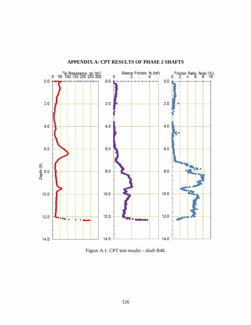
126

APPENDIX A: CPT RESULTS OF PHASE 2 SHAFTS

Figure A.1. CPT test results – shaft B48.

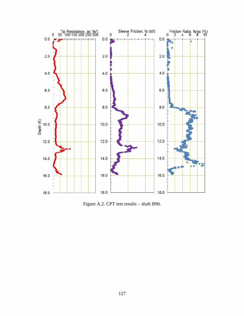
127

Figure A.2. CPT test results – shaft B96.

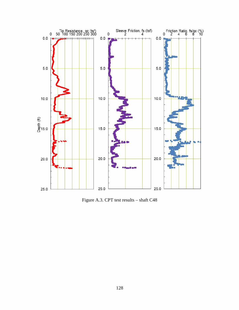
128

Figure A.3. CPT test results – shaft C48

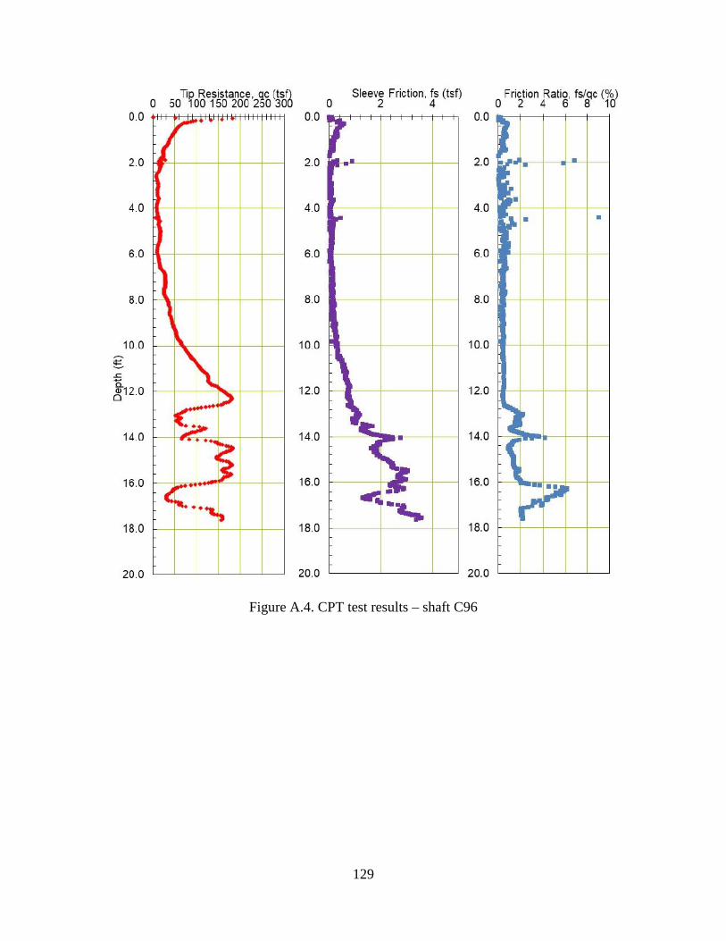
129

Figure A.4. CPT test results – shaft C96

130

Figure A.5. CPT test results – shaft K48

131

Figure A.6. CPT test results – shaft K96

132

Figure A.7. CPT test results – shaft M48

133

Figure A.8. CPT test results – shaft M96

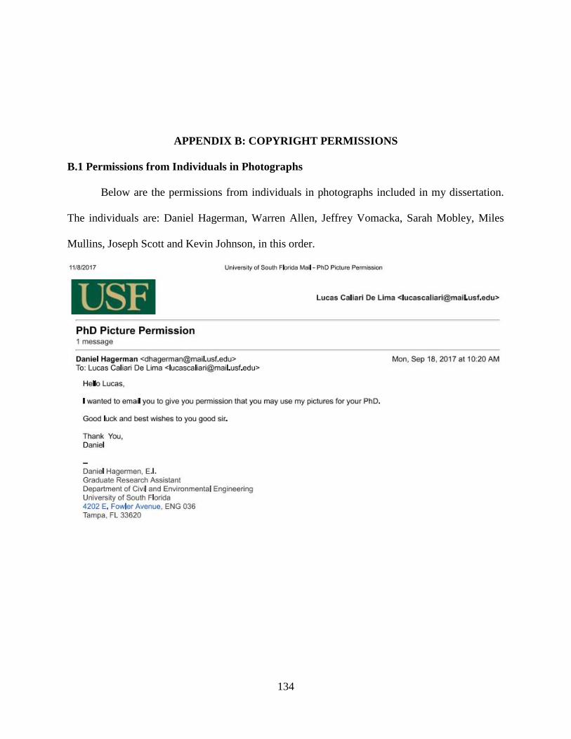
134

APPENDIX B: COPYRIGHT PERMISSIONS

B.1 Permissions from Individuals in Photographs

Below are the permissions from individuals in photographs included in my dissertation.

The individuals are: Daniel Hagerman, Warren Allen, Jeffrey Vomacka, Sarah Mobley, Miles

Mullins, Joseph Scott and Kevin Johnson, in this order.

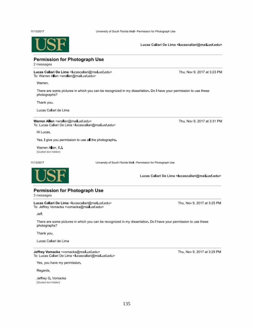
135

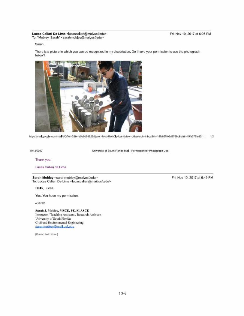
136

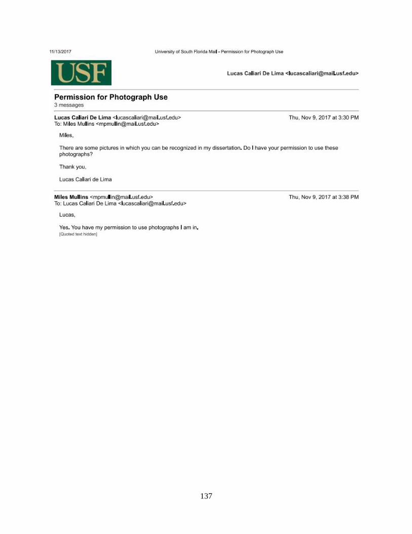
137

138

139