CONSTRUCTION COST OF UNDERGROUND INFRASTRUCTURE by …

CONSTRUCTION COST OF UNDERGROUND INFRASTRUCTURE

RENEWAL: A COMPARISON OF TRADITIONAL OPEN-CUT

AND PIPE BURSTING TECHNOLOGY

by

SEYED BEHNAM HASHEMI

Presented to the Faculty of the Graduate School of

The University of Texas at Arlington in Partial Fulfillment

of the Requirements

for the Degree of

MASTER OF SCIENCE IN CIVIL ENGINEERING

THE UNIVERSITY OF TEXAS AT ARLINGTON

December 2008

Copyright © by Seyed Behnam Hashemi

All Rights Reserved

iii

ACKNOWLEDGEMENTS

I am very grateful and would like to thank my supervisor,

Dr. Mohammad Najafi, Ph.D., P.E., Director of Center for Underground

Infrastructure Research and Education (CUIRE), for his continued great

help, encouragements, and friendship throughout the course of my

graduate studies and thesis completion. I would also like to thank my

committee members, Dr. Siamak Ardekani and Dr. John Matthys for their

valuable suggestions.

My sincere thanks to Dr. Rayman Mohamed for his help to obtain the

GIS data for the case study chapter of my research and also special

thanks to Dr. Nancy Rowe from Statistical Services Department of the

University of Texas at Arlington for her valuable guidance regarding

statistical analysis and using SAS software. I also appreciate survey

respondents and municipalities who contributed to my survey and shared

their valuable information with me (Appendix O).

I would like to express my especial appreciation to my very kind and

patient wife, Nazanin, for her continuous support all the way through my

life and education road. I will always love you.

November 17, 2008

iv

ABSTRACT

CONSTRUCTION COST OF UNDERGROUND INFRASTRUCTURE

RENEWAL: A COMPARISON OF TRADITIONAL OPEN-CUT

AND PIPE BURSTING TECHNOLOGY

Seyed Behnam Hashemi, M.S.

The University of Texas at Arlington, 2008

Supervising Professor: Mohammad Najafi

Renewal of aging underground infrastructure is a major challenge that

municipalities in North America face every day. Traditional replacement or

renewal of these underground utilities uses open-cut excavation methods that

can be disruptive to everyday life of citizens and expensive, particularly in built-

up areas and in projects with difficult ground and site conditions. In contrast,

trenchless technologies use innovative methods, materials, and equipment that

require minimum surface excavation to renew and construct aging underground

infrastructure. These new methods are considered to be more safe, cost-

effective, efficient and productive than conventional open-cut projects. However,

to select trenchless technologies in utility design, consulting engineers and utility

owners need to compare their costs with open-cut methods.

v

This research provides a basis for cost comparison of pipe bursting as a

trenchless technology and traditional open-cut method. There is a case study in

this research as an example for cost comparison of replacing the sewer pipeline

in the City of Troy, Michigan. The results of the research indicates that pipe

bursting in many cases would be less expensive than the open-cut method and

by using trenchless methods, such as pipe bursting, municipalities and utility

owners could save millions of dollars in the renewal of their of underground

pipeline systems.

vi

TABLE OF CONTENTS

ACKNOWLEDGEMENTS .................................................................................... iii

ABSTRACT .......................................................................................................... iv

LIST OF ILLUSTRATIONS ................................................................................. .ix

LIST OF TABLES ............................................................................................... xii

Chapter 1. INTRODUCTION .............................................................................................. 1

1.1 Background ................................................................................................. 1

1.2 Problem Statement ..................................................................................... 3

1.3 Objectives and Methodology ....................................................................... 5

1.3.1 Objectives ............................................................................................. 5

1.3.2 Methodology ......................................................................................... 5

1.4 Literature review ......................................................................................... 6

1.5 Expected Outcomes and Limitations ........................................................... 9

2. TRENCHLESS TECHNOLOGY AND PIPE BURSTING ................................. 11

2.1 Introduction ............................................................................................... 11

2.2 Trenchless Technology ............................................................................. 11

2.2.1 Trenchless Construction Methods (TCM) ........................................... 12

2.2.2 Trenchless Renewal Methods (TRM).................................................. 13

2.3 Pipe Bursting History ................................................................................ 14

2.4 What is Pipe Bursting? .............................................................................. 14

2.5 Insertion and Receiving Pits...................................................................... 17

2.6 Reconnection of Service ........................................................................... 18

2.7 Different Methods of Pipe Bursting ........................................................... 18

2.7.1 Pneumatic Pipe Bursting ..................................................................... 19

2.7.2 Hydraulic Expansion ........................................................................... 20

2.7.3 Static Pull ............................................................................................ 21

vii

2.8 Pipe Material ............................................................................................. 23

2.8.1 Asbestos Cement Pipe (ACP) ............................................................. 24

2.8.2 Concrete Pipe (CP) ............................................................................. 24

2.8.3 Vitrified clay pipe (VCP) ...................................................................... 24

2.8.4 Metallic Pipe ....................................................................................... 25

2.8.6 Plastic Pipe ......................................................................................... 26

2.9 Applicability of Pipe Bursting ..................................................................... 26

2.10 Advantages and Limitations .................................................................... 28

2.11 Summary ................................................................................................. 29

3. OVERVIEW OF OPEN-CUT CONSTRUCTION ............................................. 30

3.1 Introduction ............................................................................................... 30

3.2 Pipe Material ............................................................................................. 30

3.3 Trench Excavation .................................................................................... 31

3.4 Trench Wall ............................................................................................... 32

3.5 Bedding and Laying .................................................................................. 33

3.6 Embedment................................................................................................... 34

3.7 Backfill and Compaction ........................................................................... 34

3.8 Summary................................................................................................... 35

4. COST ANALYSIS OF OPEN-CUT AND PIPE BURSTING ............................. 36

4.1 Regression and Model Building ................................................................ 36

4.1.1 Simple Regression Model ................................................................... 37

4.1.2 Multiple Regression Model .................................................................. 37

4.2 Pipe Bursting ............................................................................................. 38

4.2.1 Data Collection ................................................................................... 38

4.2.2 Pipe Bursting Data Analysis ................................................................ 41

4.3 Open-Cut .................................................................................................. 52

4.3.1 Data Collection ................................................................................... 52

4.3.2 Open-Cut Data Analysis ..................................................................... 53

4.4 Comparison ............................................................................................... 65

4.5 Hypothesis Test ........................................................................................ 66

4.6 Summary................................................................................................... 69

viii

5. CASE STUDY OF PIPE BURSTING VS. OPEN-CUT .................................... 70

5.1 Pipeline Infrastructure in City of Troy, Michigan ........................................ 70

5.2 Cost Estimating for Pipe Replacement Using Bursting Method ................ 73

5.3 Cost Estimating for Pipe Replacement Using Open-Cut Method .............. 76

5.4 Cost Comparison Results and Analysis .................................................... 79

6. CONCLUSIONS AND RECOMMENDATIONS FOR FUTURE RESEARCH .. 81

6.1 Conclusions .............................................................................................. 81

6.2 Recommendations for Future Research ................................................... 83

Appendix

A. SIMPLE REGRESSION ............................................................................. 85

B. MULTIPLE REGRESSION ......................................................................... 88

C. PIPE BURSTING ACTUAL PROJECTS DATA .......................................... 91

D. PIPE BURSTING AND OPEN-CUT SURVEY ROW DATA........................ 94

E. PIPE BURSTING AND OPEN-CUT SURVEY QUESTIONAIRE .............. 101

F. ABBREVIATIONS ..................................................................................... 106

G. SAS CODES FOR PIPE BURSTING MODEL ......................................... 108

H. SAS DATA MATRIX FOR PIPE BURSTING ............................................ 111

I. SAS MATRIX METHOD OUTPUT FOR PIPE BURSTING MODEL .......... 113

J. SAS CODES FOR OPEN-CUT MODEL ................................................... 115

K. SAS DATA MATRIX FOR OPEN-CUT ..................................................... 118

L. SAS MATRIX METHOD OUTPUT FOR OPEN-CUT MODEL .................. 120

M. PIPE BURSTING REGRESSION CALCULATION .................................. 122

N. OPEN-CUT REGRESSION CALCULATION ............................................ 124

O. SURVEY RESPONDENTS ...................................................................... 126

REFERENCES ................................................................................................. 128

BIOGRAPHICAL INFORMATION ..................................................................... 131

ix

LIST OF ILLUSTRATIONS Figure Page

1.1 U.S. sanitary and storm sewer systems survey coverage …… 4 1.2 Cost identification for underground utility project ………..……. 7 2.1 Typical pipe bursting operation layout………………………...... 16 2.2 Pneumatic, hydraulic and static head ………………………….. 19

2.3 Bursting head of the pneumatic system………………………... 19

2.4 Hydraulic bursting head (Xpandit) in

expanded and contracted positions…………………………….. 21

2.5 Bursting head of the static pull system…………………………. 22 3.1 Open-Cut trench width requirement…………………….……….32

3.2 Site clearance for trench walls a) Vertical trench wall and b) Sloping trench wall……….......... 33 3.3 Open-Cut trench cross section view.……………………………. 35 4.1 Scatter plots of pipe bursting data (a) Cost versus pipe diameter size and (b) cost versus length of project ……... 41

4.2 Fit trend line on pipe bursting cost and diameter data (a) linear (b) logarithmic (c) power (d) exponential regression.. 42 4.3 Fit trend line on pipe bursting cost and length data (a) linear (b) logarithmic (c) power (d) exponential regression.. 44

4.4 SAS scattered plot of pipe bursting data (a) cost vs. diameter size (b) cost vs. length (c) cost vs. length square (d) cost vs. logarithm of diameter (e) cost vs. logarithm of length…………... 46

4.5 Fit Analysis of the length and diameter variables………………. 47

4.6 Fit Analysis of the length, diameter, and L2 variables…………. 48

x

4.7 Fit Analysis of the length, L2, and LD variables………………… 49

4.8 Fit Analysis of the length, diameter, L2, LD, and LL variables………………………………………….. 50

4.9 Scatter plots of open-cut data (a) Cost versus pipe diameter size (b) cost versus length of project……………. 54

4.10 Fit trend line on cost and diameter size of open-cut data (a) linear (b) logarithmic (c) power (d) exponential regression... 55

4.11 Fit trend line on cost and length of open-cut data (a) linear (b) logarithmic (c) power (d) exponential regression... 57

4.12 SAS scattered plot of open-cut data (a) cost vs. diameter size (b) cost vs. length (c) cost vs. length square (d) cost vs. logarithm of diameter (e) cost vs. logarithm of length…….. 59

4.13 Fit Analysis of the length and diameter variables……………… 60

4.14 Fit Analysis of the length and LD variables…………………….. 61

4.15 Fit Analysis of the LD and LL variables…………………………. 62

4.16 Fit Analysis of the LD and LL variables…………………………. 63

4.17 Comparison of trend lines of open-cut and pipe bursting (a) open-cut price vs. diameter (b) pipe bursting price vs. diameter (c) open-cut price vs. length (d) pipe bursting price vs. length…………………….……………………………...... 65

5.1 Location of City of Troy in State of Michigan…………………… 71

5.2 Sewer Pipeline Layout of City of Troy in State of Michigan…………………………………………. 71

5.3 Estimated Sewer Pipeline Replacement Cost Comparison for City of Troy………………………………………. 79

xi

LIST OF TABLES Table Page

2.1 Trenchless Technology Methods………………...……………… 12

4.1 Pipe Bursting Data ………………………………………………. 39

4.2 Cost vs. Diameter, Trend Lines Comparison………………….. 43 4.3 Cost vs. Length, Trend Lines Comparison…………………….. 44

4.4 Comparison of Different Multiple Regression Lines…………. 51

4.5 Open-Cut Data……………………………………………………. 52

4.6 Cost vs. Diameter, Trend Lines Comparison………………….. 56 4.7 Cost vs. Length, Trend Lines Comparison…………………….. 57

4.8 Comparison of Different Multiple Regression Lines…………. 64 4.9 Average and Standard Deviation for Pipe Bursting Data ……. 67 4.10 Average and Standard Deviation for Open-Cut Data….. ……. 68

5.1 City of Troy Sewer Pipeline Information……………………….. 72 5.2 Estimation of Pipe Bursting Cost

by Multiple Regression…………………………………………… 73

5.3 Estimation of Pipe Bursting Cost Per Foot Per Inch …………. 74

5.4 Estimation of Open-Cut Cost by Multiple Regression………… 76

5.5 Estimation of Open-Cut Cost Per Foot Per Inch………………. 77 5.6 City of Troy Sewer Pipeline Replacement Cost Comparison…………………………………………………. 80

1

CHAPTER 1

INTRODUCTION

1.1 Background

A large amount of the underground infrastructure currently in use in the

North America was the result of the postwar construction rise started by fast

growth of the economies of Canada and the United States in the 1950s and

1960s. During this period, most of today’s infrastructure utilities such as water,

sewer, gas, and power were developed. Now, these systems on the average are

more than 70 years old, have exceeded their design lives, and have deteriorated

to the point that their failures have become a common everyday news item.

It is estimated that the water and wastewater industry needs from $150

billion to $2 trillion for next 20 years (Najafi and Gokhale, 2005). American

Society of Civil Engineers (ASCE) estimates that it will cost $1.3 trillion just to

maintain current underground infrastructure systems for the next five years.

As a result of deterioration of municipal underground infrastructure

systems and a growing population that demands better quality of life, the efficient

and cost effective installation, renewal, and replacement of underground utilities

is becoming an increasing important issue. The traditional open-cut construction

method requires reinstatement of the ground surface, such as sidewalks,

pavement, landscaping; and therefore, considered to be a wasteful operation.

2

Additionally, considering social and environmental factors, open-cut methods

have negative impacts on the community, businesses, and commuters due to

surface and traffic disruptions. Trenchless technologies include all methods of

underground utility installation, replacement and renewal without or with

minimum surface excavation. These methods can be used to repair, upgrade,

replace, or renovate underground infrastructure systems with minimum surface

disruptions, and therefore offer a viable alternative to the traditional open-cut

methods.

The total cost of every pipeline project varies with many factors such as

pipe size, pipe material, depth and length of installation, project site, subsurface

conditions, and type of pipeline or utility application. With open-cut construction, it

is estimated that approximately 70 percent of a project’s direct costs will be spent

for reinstatement of ground only, not installation of the pipe itself (Najafi and

Gokhale, 2005).

An established form of trenchless construction is pipe bursting. ASCE

Pipe Bursting Manual (2006) defines pipe bursting as “… a replacement method

in which an existing pipe is broken by brittle fracture, using mechanically applied

force from within. The pipe fragments are forced into the surrounding ground. At

the same time, a new pipe of the same or larger diameter is drawn in, replacing

the existing pipe. Pipe bursting involves the insertion of a conically shaped tool

(bursting tool) into the existing pipe to shatter the existing pipe and force its

fragments into surrounding soil by pneumatic or hydraulic action. A new pipe is

pulled or pushed in behind the bursting head.”

3

In the engineering community, there is usually hesitation and resistance in

accepting new technologies. This might be due to a number of reasons, such as

risk and uncertainty involved, unfamiliarity with the new technology, and most of

all, a misconception that the new technologies definitely would cost more than

the traditional ones. Although there have been several preliminary studies

regarding the cost comparison of trenchless with open-cut method, more detailed

cost comparison will be helpful in acceptance of these new technologies. In this

research, we will specifically compare cost of open-cut and pipe bursting as a

trenchless technology method by use of surveys, case studies and statistical

analysis..

1.2 Problem Statement

Traditional open-cut construction method includes direct costs that

greatly increase by the need to restore ground surfaces such as sidewalks,

pavement, and landscaping. Additionally, considering social and environmental

factors into the comparison, open-cut methods have negative impacts on the

communities, businesses, and commuters due to surface and traffic disruptions.

In comparison, trenchless technologies can be used to repair, upgrade, replace,

or install underground infrastructure systems with minimum surface disruptions

and offer a viable alternative to existing open-cut methods. When new

technologies and methods are considered as alternative construction methods,

there is usually hesitation and resistance in accepting the new technology mainly

due to unknown cost parameters.

4

Najafi and Gokhale (2005) state that the total U.S. sanitary and storm

sewer system includes 5,200,000,000 ft (approximately 985,000 miles) of pipe.

Based on the U.S. sanitary and storm sewer systems survey concluded by

Hashemi and Najafi (2007), it is estimated that about 9 percent of the U.S. total

existing sewer pipeline systems is in poor conditions and needs to be replaced.

Figure 1.1 shows the coverage of this survey throughout the United States. If we

apply the result of this survey, (0.09 x 5,200,000,000 ft), there would be

approximately 468,000,000 ft or approximately 90,000 miles of pipeline that

currently is in need of replacement. This problem would be more critical, if

deteriorated water, gas, and oil pipelines are also added to the sewer estimates.

Figure 1.1 U.S. sanitary and storm sewer systems survey coverage (Hashemi & Najafi, 2007)

Although there have been several studies regarding the cost comparison

of trenchless with open-cut methods, a more detailed cost comparison study will

be helpful in acceptance of these new technologies.

5

1.3 Objectives and Methodology

1.3.1 Objectives

The first objective of this research is development of a model for cost

comparison of pipe bursting and open-cut method. Our hypothesis is that pipe

bursting would cost much less than traditional open-cut method. The second

objective is to examine the model developed in the first objective to illustrate cost

benefits of pipe bursting.

1.3.2 Methodology

The methodology for this research is literature search, survey of

municipalities and industry professionals and preliminary statistical analysis using

regression method. Regression method is a technique that has ability to figure

out the relationship between one parameter as a function of one or more

variables. In this research, price per foot of pipe bursting and open-cut is used as

“y” parameter and length and diameter size of pipeline project is used as “x”

variables.

While limited data reduces reliability of regression analysis presented,

nevertheless, this research safely concludes that the cost of the pipe bursting

method is significantly less than the open-cut method. This cost saving will

consequently save municipalities millions of dollars in the renewal of their

underground utilities systems.

6

1.4 Literature review

According to Jung and Sinha (2007), there are various costs related

to a renewal pipeline project either with open-cut or pipe bursting. The authors

considered some parameters related to these kinds of projects; namely, direct,

social, and environmental. They asserted that the interrelation among these

costs is becoming more important with growing public awareness of societal and

environmental issues. They provided two general formulas for open-cut and

trenchless methods as:

TCOC = CDIRECT + CSOCIAL + CENVIRONMENTAL + COTHER FACTORS

TCTT = CDIRECT + CSOCIAL + CENVIRONMENTAL + COTHER FACTORS.

Where:

TCOC = total cost of open-cut method

TCTT = total cost of trenchless technology

CDIRECT = earthwork cost, restoration cost, overhead cost, and so on

(including material, labor, and equipment cost).

CSOCIAL = traffic delay cost, income loss of business, and so on.

CENVIRONMENTAL = noise pollution cost, air pollution cost, and so on. COTHER

FACTORS = productivity loss cost, safety hazard cost, structural behavior

cost, and so on.

The authors concluded that with above parameters, pipe bursting as a

trenchless method would be less expensive than open-cut technique. However,

they did not consider any actual project data for prediction of the pipe bursting or

open-cut costs.

7

Woodroffe and Ariaratnam (2008) presented a comparison of risk factors

of another trenchless technology technique called horizontal directional drilling

(HDD) and compared those factors with traditional open cut applications. They

found that HDD can minimize risks and reduce the overall costs of construction in

an urban environment. The main concentration of their research was based on

risk factors shown in Figure 1.1, however; they failed to present a cost analysis of

the two methods.

Figure 1.2 Cost identification for underground utility project (Woodroffe & Ariaratnam, 2008)

Najafi and Kim (2004) presented an investigation of parameters involved

in constructing underground pipelines with trenchless methods in urban centers

in comparison with conventional open-cut method. Their study included a

breakdown of the engineering and capital costs of the construction and the social

costs for both methods. They considered life-cycle cost of a project with the point

of view of pre-construction, construction, and post-construction parameters. They

8

asserted that considering the life-cycle costs of a project, innovative methods and

trenchless technology are more cost-effective than traditional open-cut method.

Although the authors considered cost parameters for both trenchless and open-

cut methods, they did not consider an actual cost data analysis for comparison of

these two methods. Such actual cost anaysis is the main consideration of this

thesis.

Gangavarapu (2003) presented a case study to compare traffic and road

disruption costs during utility construction when open-cut and trenchless

construction methods are used. The author presented a breakdown of social

costs involved in utility construction. He investigated traffic flow rates and

patterns during two sample utility construction projects to analyze the impact of

construction on the traffic flow. Using traffic delay estimates obtained from the

traffic flow and length of detoured roads, he developed a flow chart for estimating

costs of traffic disruption. He did not consider costs due to damage to pavement,

environmental impacts, safety issues, and noise and dust in his study. Although

he considered important social costs of a utility project, he did not compared

direct cost of open-cut with trenchless techniques which is the main subject of

this thesis.

Adedapo (2007) has verified and compared the impact of traditional open-

cut method and horizontal directional drilling (HDD) as a trenchless technology

method on the life of pavement structure. He considered deteriorating aspects of

open-cut construction to asphalt pavement and concluded that HDD would cause

less damage to the pavement than open-cut. His focus in this research was more

9

on physical aspects of two methods and did not cover cost aspects. In this thesis,

the focus is on cost comparison of open-cut and pipe bursting methods.

Atalah (2004) has studied interaction between pipe bursting and

surrounding soil especially in sand and gravel with the goal of comparing the cost

effectiveness of pipe bursting versus open-cut. He studied a comparison of

these two methods based on soil characteristics. He did not concentrate on the

relationship between cost as a function of pipe diameter and length for open-cut

and pipe bursting methods which is the main focus of this thesis.

1.5 Expected Outcomes and Limitations

Our hypothesis is that the trenchless pipe-bursting method would be less

expensive than the open-cut method for replacing the underground sewer

pipelines. Among other factors, the open-cut method mainly requires continuous

excavation and often expensive trench-wall protective systems all along the

pipeline alignment, while trenchless technology requires only the excavation at

entry and exit pits which are located at widely spaced intervals. Therefore, we

expect to conclude that using trenchless methods instead of open-cut excavation

can save municipalities millions of dollars in the renewal of their underground

utilities systems.

With regard to the open cut method, our sample size is small with only

cost data for 9 projects. We understand the constraints of limited data but for the

sake of calculation and cost comparisons with pipe bursting where we obtained

more data, decided to continue with our regression analysis. In reality, project

10

specific conditions including surface and subsurface differences, prohibit any

scientific cost comparison between two methods.

For the purpose of case study presented in this research, we assume the

entire sewer pipeline in the City of Troy, Michigan, would be replaced at the

same time. In reality, the replacement process will be dependent on the age and

conditions of specific pipeline sections, along with many other factors. Therefore,

the total budget estimated for this case study would in fact incur over a period of

time.

Another assumption for this study is that all replacement and renewal work

will be conducted with pipe bursting, while in reality it may be performed using

other trenchless technology methods (such as cured-in-place pipe or CIPP,

sliplining, close-fit-pipe, point repair, and so on) or a new pipeline may be

installed with such methods as microtunneling or horizontal directional drilling.

It should be noted that pipe bursting is the only trenchless renewal method

capable of increasing diameter of an existing pipe, which makes it more suitable

for conditions where existing pipe has inadequate hydraulic capacity and/or

future growth is expected. Another limitation of this research is that for the City of

Troy, the case of study does not consider service laterals which would add some

costs to the pipe bursting option.

11

CHAPTER 2

TRENCHLESS TECHNOLOGY AND PIPE BURSTING

2.1 Introduction

Trenchless Technology is a new alternative for traditional installation or

replacement of the underground infrastructure with minimal disruption to surface

and subsurface. Advantages of these methods are fewer trenches,

environmentally friendly construction operations, cost-effectiveness, and a better

level of safety and productivity in the construction process. This technology

branches to different techniques and methods mainly in two groups of new

installation and replacement of old pipelines. Pipe Bursting is one of the

replacement methods that will be described in this chapter.

2.2 Trenchless Technology

North American Society for Trenchless Technology (NASTT) defines

trenchless technology as a family of methods, materials, and equipment capable

of being used for the installation of new or replacement or rehabilitation of

existing underground infrastructure with minimal disruption to surface traffic,

business, and other activities. Trenchless technology methods are divided into

two main categories; Trenchless Construction Methods (TCM) and Trenchless

Renewal Methods (TRM), as shown in Table 2.1.

12

Table 2.1 Trenchless Technology Methods

Trenchless Technology Methods

Trenchless Construction Methods (TCM)

Trenchless Renewal Methods (TRM)

Utility Tunneling Cured-In-Place Pipe

Pipe Jacking Pipe Bursting

Horizontal Auger Boring Close-fit Pipe

HDD Thermoformed Pipe

Microtunneling Sliplining

Pipe ramming In-line Replacement

Pilot Tube Microtunneling Localized repair

Lateral renewal

Coating & Linings

Manhole renewal

2.2.1 Trenchless Construction Methods (TCM)

First group of trenchless technology methods as shown in Table 2.1 is

TCM for installation of new pipelines. Table 2.1 also divides TCM into major

methods: utility tunneling (UT), pipe jacking (PJ), horizontal auger boring (HAB),

horizontal directional drilling (HDD), microtunneling, pipe ramming and pilot tube

microtunneling (PTMT). Both PJ and UT techniques require workers inside the

tunnel during excavation and pipe and/or temporary-support installation process.

Nonetheless, PJ is different from UT by the support structure. PJ technique uses

installation of pre-manufactured pipe sections during the tunnel excavation. In

this method, new pipe sections are jacked from a drive shaft so that the complete

string of pipe is installed simultaneously with the excavation of the tunnel (Najafi

13

and Gokhale, 2005). In UT, first a support liner is installed during the tunnel

excavation and then the pipe sections are transported and placed inside the

tunnel.

2.2.2 Trenchless Renewal Methods (TRM)

Second group of trenchless technology techniques shown in Table 2.1 is

TRM. TRM includes methods for replacing, rehabilitating, renewing, or upgrading

(collectively called renewal methods) the existing pipeline systems. The renewal

methods can also be used to replace and enlarge existing pipelines. The term

renewal is used when trenchless methods are applied to extend the design life of

pipelines however; the term repair is used when the trenchless methods are used

to repair existing pipelines without extending their design life.

According to Najafi and Gokhale (2005), the selection of trenchless

pipeline renewal methods depends on the physical conditions of the existing

pipeline system, such as pipeline length, type of material, size, type and number

of manholes, service connections, bends, and the nature of the problem or

problems involved. The problems with an existing pipe may include structural or

nonstructural, infiltration or inflow, ex-filtration or outflow, pipe breakage, joint or

pipe misalignment, capacity, corrosion and abrasion problems, and so on. Other

features of the renewal systems such as applicability to a specific project,

constructability, cost factors, availability of service providers, life expectancy of

new pipe, and future use of pipe should also be considered. Table 2.1 shows the

different TRMs which includes pipe bursting. The following sections of this

14

chapter describe pipe bursting method in detail as in this research pipe bursting

is selected for cost comparison of trenchless method with open-cut technique.

2.3 Pipe Bursting History

Pipe bursting was first developed in the UK in the late 1970s by D. J. Ryan

& Sons in conjunction with British Gas, for the replacement of small diameter, 3

and 4 in. cast iron gas mains (ASCE 2006). The pipe bursting process at the time

involved a pneumatically drive, cone-shaped bursting head operating by a

reciprocating impact process. This method was patented in the U.K. in 1981 and

in the United States in 1986. While the original patents expired in April 2005, new

proprietary pipe bursting methods have been developed and patented. When it

was first introduced, this method was used only in replacing cast iron gas

distribution pipes; and later was developed for replacing water and sewer lines.

The total footage of pipe replaced using pipe bursting in the United States is

growing at approximately 20% per year, the majority of which is for sewer line

replacement (ASCE 2006).

2.4 What is Pipe Bursting?

Based on ASCE (2006) Pipe Bursting Manual, pipe bursting is defined as

a replacement method in which an existing pipe is broken by brittle fracture,

using mechanically applied force from within. The pipe fragments are forced into

15

the surrounding ground. At the same time, a new pipe of the same or larger

diameter is drawn in, replacing the existing pipe.

In a pipe bursting operation (Figure 2.1), a cone-shaped tool, bursting

head, is inserted into the existing pipe and forced through it and fracture the pipe

and push its fragments into the surrounding soil. At the same time, a new pipe is

pulled or pushed in the annulus left by the expanding operation (depending on

the type of the new pipe). In majority of pipe bursting operations, the new pipe is

pulled into place. The new pipe can be of the same size or larger than the

replaced pipe. The rear of the bursting head is connected to the new pipe, and

the front end of the bursting head to either a winching cable or a pulling rod

assembly.

The bursting head and the new pipe are launched from an insertion pit.

The cable or rod assembly is pulled from the pulling or reception pit. The leading

or nose portion of the bursting head is often smaller in diameter than the existing

pipe, to maintain alignment and to ensure a uniform burst. The base of the

bursting head is larger than the inside diameter of the existing pipe to be burst, to

fracture it. The head is also slightly larger than the outside diameter of the

replacement pipe, to reduce friction on the new pipe and to provide space for

maneuvering the pipe. The bursting head can be additionally equipped with

expanding crushing arms, sectional ribs, or sharp blades, to further promote the

bursting efficiency.

16

Figure 2.1 Typical pipe bursting operation layout (Simicevic & Sterling, 2001)

Sometimes an external protective covering pipe is installed during the

bursting process and the product pipe installed within this casing or conduit pipe.

This is usually only considered for pressure pipe installations. Alternatively, in

gravity sewer applications, the wall thickness of the product pipe is increased to

allow for external scaring of the pipe as it is pulled into the place. The bursting

operation can proceed either continuously or in steps, depending on the applied

type of pipe bursting system. Before bursting, to reduce the required pull force,

the existing pipe should always be cleaned and any sand or debris is removed,

as well as all the service connections located and disconnected.

Many factors should be reviewed thoroughly before pipe bursting projects

are considered and released for bid. Engineers should consider different options

and select the most cost effective and environmentally friendly methods for bid.

The method selection should not be left to only to the judgment of the contractor.

Pipe bursting is especially cost effective if the existing pipe is out of capacity.

There are, however, limits to the use of the pipe bursting method, and various

17

conditions challenge the successful use of its application which are presented in

section 2.10 of this chapter.

Pipe bursting techniques are most advantageous in cost terms when:

there are few lateral connections to be reconnected within a replacement section,

the old pipe is structurally deteriorated, additional capacity is needed, or

restoration/environmental mitigation requirements are difficult.

2.5 Insertion and Receiving Pits

According to ASCE pipe bursting manual (2006), insertion (new pipe entry

point) and receiving pits should be strategically and safely located to reduce the

overall excavation on a project, considering the traffic flow and specific conditions

of a project. Normally, water main systems have clusters of gate valves at street

intersections and fire hydrants at intervals of 500 ft or less. Trunk sewer systems

commonly have manholes at intervals of 400 to 500 ft or less. These should be

prime locations for pits because valves, hydrants, and manholes are usually

replaced with the pipe. In general, the material, diameter, and diameter thickness

ratio (DR) of the new pipe will determine the length of the entry pit required.

Over-bending the pipe can cause overstressing the pipe material and create

damage which may not become apparent until the pipe is in operation. The width

of the pit is dependent on the pipe diameter and OSHA confined space or

shoring requirements. The use of appropriate pit shoring is defined by depth and

ground conditions as described in OSHA regulations.

18

2.6 Reconnection of Service

According to the ASCE Pipe Bursting Manual (2006), the reconnection of

service, sealing of the annular space at the manhole location, or backfilling of the

insertion pit for new polyethylene (PE) pipe must be delayed for the pipe

manufacturer’s recommended time, but normally not less than 4 hours. This

period allows for PE pipe shrinkage due to cooling and pipe relaxation owning to

the tensile stresses inducted in the pipe during installation. Following the

relaxation period, the annular space in the manhole wall may be sealed. Sealing

is extended a minimum of 8 in. into a manhole wall in such a manner as to form a

smooth, watertight joint. Ensuring a proper bond between the polyvinyl chloride

(PVC) or PE replacement pipe and the new manhole wall joint is critical.

Service connections can be reconnected with specially designed fittings

by various methods. The saddles, made of a material compatible with that of new

pipe, are connected to create a leak-free joint. Different types of fused saddles

(electrofusion saddles, conventional fusion saddles) are installed in accordance

with manufacturer’s recommended procedures. Connection of new service

laterals to the pipe also can be accomplished by compression-fit service

connections. After testing and inspection to ensure that the service meets all the

required specifications of the service line, the pipeline returns to service.

2.7 Different Methods of Pipe Bursting

According to Simicevic and Sterling (2001), currently available pipe

bursting systems which is based on the type of bursting head used, can be

classified into three main classes (Figure 2.2):

19

(1) Pneumatic pipe bursting

(2) Hydraulic expansion

(3) Static pull

Figure 2.2 From left to right, pneumatic, hydraulic and static head

(Simicevic & Sterling, 2001)

2.7.1 Pneumatic Pipe Bursting

In the pneumatic pipe bursting, the bursting head is a cone-shaped soil

displacement hammer. It is driven by compressed air, and operated at a rate of

180 to 580 blows /minute. As Figure 2.3 shows, a small pulling device guides the

head via a constant tension winch and cable. Hydraulic head expands and closes

sequentially as it is pulled through the pipe, bursting the pipe on its way. Static

head has no moving internal parts. The head is simply pulled through the pipe by

a heavy-duty pulling device via a segmented drill rod assembly or heavy anchor

chain.

Figure 2.3 Bursting head of the pneumatic system (Simicevic & Sterling, 2001)

20

The percussive action of the bursting head is similar to hammering a nail

into a wall, where each impact pushes the nail a small distance farther into the

wall. In a like manner, the bursting head creates a small fracture with every

stroke, and thus continuously cracks and breaks the old pipe.

The percussive action of the bursting head is combined with the tension

from the winch cable, which is inserted through the old pipe and attached to the

front of the bursting head. It keeps the bursting head pressed against the existing

pipe wall, and pulls the new pipe behind the head.

The air pressure required for the percussion is supplied from the air

compressor through a hose, which is inserted through the new pipe and

connected to the rear of the bursting tool. The air compressor and the winch are

kept at constant pressure and tension values respectively. The bursting process

continues with little operator intervention, until the bursting head comes to the

reception pit.

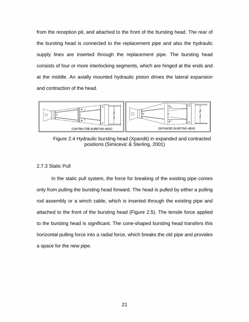
2.7.2 Hydraulic Expansion

In the hydraulic expansion system, the bursting process advances from

the insertion pit to the reception (pulling) pit in sequences, which are repeated

until the full length of the existing pipe is replaced. In each sequence, one

segment of the pipe (which matches the length of the bursting head) is burst in

two steps: first the bursting head is pulled into the old pipe for the length of the

segment, and then the head is expanded laterally to break the pipe. The bursting

head is pulled forward with a winch cable, which is inserted through the old pipe

21

from the reception pit, and attached to the front of the bursting head. The rear of

the bursting head is connected to the replacement pipe and also the hydraulic

supply lines are inserted through the replacement pipe. The bursting head

consists of four or more interlocking segments, which are hinged at the ends and

at the middle. An axially mounted hydraulic piston drives the lateral expansion

and contraction of the head.

Figure 2.4 Hydraulic bursting head (Xpandit) in expanded and contracted positions (Simicevic & Sterling, 2001)

2.7.3 Static Pull

In the static pull system, the force for breaking of the existing pipe comes

only from pulling the bursting head forward. The head is pulled by either a pulling

rod assembly or a winch cable, which is inserted through the existing pipe and

attached to the front of the bursting head (Figure 2.5). The tensile force applied

to the bursting head is significant. The cone-shaped bursting head transfers this

horizontal pulling force into a radial force, which breaks the old pipe and provides

a space for the new pipe.

22

Figure 2.5 Bursting head of the static pull system (Simicevic & Sterling, 2001)

If a rod assembly is used for pulling, the bursting process is done in

consecutive sequences, rather than continuously. Prior to bursting, the

segmented rods are inserted into the old pipe from the reception pit. The rods are

only a few feet long, and during insertion they are threaded together to reach the

bursting head at the insertion pit. The rods are attached to the front end of the

bursting head, and the new pipe is connected to its rear end. In each sequence

during the bursting, the hydraulic unit in the reception pit pulls the rods for the

length of individual rods, and the rods are separated from the rest of rod

assembly as they reach the reception pit. If a winch cable is used instead of rods,

the pulling process can be continuous. However, a typical cable system does not

transmit as a large pulling force to the bursting head as a rod assembly.

23

2.8 Pipe Material

According to ASCE Pipe Bursting Manual (2006), most existing pipe

materials used for water, wastewater, and natural gas piping systems are

candidates for bursting using present replacement methodologies. Nonetheless,

there are some circumstances where an existing pipeline may not be a good

applicant for bursting due to the surrounding soil environment of the pipe, such

as when pipe installed in a rock trench, backfilled with concrete or certain other

fill encasement, or a pipeline at a shallow depth. In addition, there are some

types of pipe materials for which technology is not presently available for

fracturing, splitting, or otherwise displacing the burst pipe or its fragments in to

the nearby soil.

Therefore, the first step in evaluating the compatibility of a given piping

system using pipe bursting replacements is to evaluating the concerns related to

the existing pipe and its soil environment. Existing pipe materials are considered

fracturable if the pipe experiences breakable disastrous crash when subjected to

a radial increasing (or tensile) force. In most cases, fracture and expand pipe

materials have mechanical properties which are either very low in tensile yield

strengths or have very low elongation characteristics (they are brittle). Pipe

materials with these properties are good candidates for pipe bursting. They

include ACP, CP, RCP, PCP, VCP, and CIP∗.

∗ Appendix F shows abbreviations

24

2.8.1 Asbestos Cement Pipe (ACP)

Asbestos cement pipe generally used in water and not often in sewer

application in the United States until a controversial U.S. Although ACP is

structurally a good candidate for pipe bursting/replacement, the owner and

engineer must investigate any federal, state, or local regulations may consider

burst asbestos pipe a potential hazard, even when left underground and outside

the new pipe.

2.8.2 Concrete Pipe (CP)

Concrete pipe is designed as a rigid conduit where the external earth

loads are designed to be transferred through the pipe wall into the soil

underneath the pipe. Thus, standard CP is ideally suitable for the pipe

bursting/replacement process, during which the bursting cone generates tensile

stresses within the walls the pipe, causing fracture of the existing pipe.

RCP and other pressure cylinder pipes, nonetheless, incorporate a steel

reinforcing cage or solid steel cylinders on the inside of the pipe for addressing

loading conditions a significant increase in tensile capability (e.g., relatively large

pipe diameter, increases in burial depth, or both). This steel limits the number of

bursting systems that can be used for replacing this type of pipe (ASCE Pipe

Bursting Manual, 2006).

2.8.3 Vitrified clay pipe (VCP)

Vitrified clay pipe is one of the most essentially static pipe materials

available which is good resistant to a broader range of PH values and

25

contaminants than any other pipe material. Due to its excellent compression

strength and poor tension characteristics, VCP is also designed as a rigid

conduit. The manufacturing process for VCP prohibits the use of secondary steel

reinforcement which, in combination with the relatively low tensile strength and

lack of ductility of this ceramic pipe, renders this material the ideal candidate for

pipe bursting/ replacement. Similar to CIP, VCP generally breaks off in slabs

which, in yielding soil trenches where the existing pipe fragments can be properly

expanded, do not normally tend to damage new plastic pipes during the

replacement process. It is important that scratching or gouging is not generally a

concern for long-term performance of pipes other than plastic pipes such as

HDPE or PVC (ASCE Pipe Bursting Manual, 2006).

2.8.4 Metallic Pipe

Existing metallic pipes for sewer applications will generally include Ductile

Iron Pipe (DIP) or steel pipe with smooth-wall and corrugated. They have almost

the same mechanical properties. With a minimum tensile strength of 60,000 psi

and a minimum elongation of 10%, metallic pipes are clearly some of the most

difficult material for bursting. In addition, there is the possibility that the axial slit/

split, cut into the wall of either DIP or steel pipe prior to the expansion, may

present sharp edges to the replacement pipe. During a large upsizing, this

condition may detract from the long-term performance of plastic pipe due to

external scouring, cutting, or gouging of the pipe wall. Such external damage

would have a much greater impact on plastic pressure pipe than on plastic

gravity service piping applications. In order to reduce such occurrences, the pipe

26

burst operation should be limited to size-on-size or to an increase of only one

nominal size (ASCE Pipe Bursting Manual, 2006).

2.8.6 Plastic Pipe

Most well-known plastic pipes would be fiberglass, High Density

Polyethylene (HDPE), and Poly Vinyl Chloride (PVC). Filament wound fiberglass

pipe can have tensile strengths on the same order of magnitude as metallic

pipes. Therefore, these pipes typically require the process of slitting/splitting prior

to expanding. Nonetheless, random oriented fiberglass pipe, such as reinforced

plastic mortar pipe, may be burst by expansion. Due to their high ductility

personality, existing HDPE and PVC pipes also require slitting/splitting prior to

replacement. HDPE pipe may be installed by any of the bursting systems,

including pneumatic, static pull, hydraulic expansion, and pipe splitting.

Equipment is available for installation of pipe up to 54 in. in diameter. HDPE

pipes through 36-in. diameter are installed on a regular basis. To facilitate

inspection of gravity flow pipes, gray-colored HDPE pipe is available. Black

HDPE with a white inner lining is also available at an added cost (ASCE Pipe

Bursting Manual, 2006).

2.9 Applicability of Pipe Bursting

Pipe bursting can be applied on a wide range of pipe sizes and types, in a

variety of soil and site conditions. The size of pipes being burst typically ranges

from 2 to 48 inches, although some projects have used larger diameters (e.g.,

80-inch) and more sizes will be possible with larger equipment in the future. The

27

most common pipe bursting method is size-for-size, or upsizing the diameter of

the existing pipe up to three sizes (e.g. 8-inch to 12-inch). Large upsizing require

more energy and may cause more ground movement. The larger sizes slow the

replacement operation and need careful evaluation and project planning

(Simicevic & Sterling, 2001).

With respect to the type of existing pipe, the pipes suitable for pipe

bursting are typically made of brittle materials, such as vitrified clay, cast iron,

plain concrete, asbestos, or some plastics. Reinforced concrete pipe (RCP) can

also be successfully replaced, if it is not heavily reinforced, or if it is substantially

deteriorated. Ductile iron and steel pipes are not suitable for pipe bursting, but

can be replaced using pipe splitting.

According to ASCE Pipe Bursting Manual (2006), two types of concrete

pressure pipe manufactured using multiple components are not economically

feasible to burst using existing technologies. These include prestressed concrete

pipe (both with and without a steel cylinder) and bar-wrapped concrete cylinder

pipe. Historically, the smallest-sized pipes for these materials have been 16-in

and 12-in., respectively, with secondary wraps of either high-strength pre

stressing wire or mild steel rod. It is this combination of a steel cylinder with wire

or rod that prevents technologies from successfully bursting/replacement such

pipes.

Simicevic and Sterling (2001), state that the bursting length is usually

between 300 and 400 feet, which is a typical distance between sewer manholes.

However, much longer bursts may be achieved when needed. A long burst

28

generally requires more powerful equipment to complete the job. The longest

continuous pipe reaming replacement was 1,320 ft (Nowak Pipe Reaming).

2.10 Advantages and Limitations

According to Atalah (2004), the pipe bursting has considerable

advantages over open cut replacements; it is much faster, more efficient, and

often cheaper than open cut especially in sewer line replacement because of the

depth of sewer lines. The increased sewer depth requires extra excavation,

shoring, and dewatering which substantially increases the cost of open cut

replacement. The increased depth has a minimal effect on the cost of pipe

bursting. Furthermore to the direct cost advantage of pipe bursting over open cut,

pipe bursting has many indirect cost savings such as less road or lane closing,

less time for replacement, less business interruption, and less traffic disturbance

than open-cut method.

Atalah (2004) asserts that the exclusive benefit of pipe bursting over

other trenchless techniques; such as CIPP, sliplining, and so on, is the ability to

upsize the service lines so that a 41% upsizing doubles the capacity of the sewer

line without considering the impact of the smoother surface of the new pipe. Pipe

bursting technique is most advantageous compared to the other trenchless

techniques in cost terms when there are few lateral connections to be

reconnected within a replacement section, when the old pipe is structurally

deteriorated, when additional capacity is needed.

29

Pipe bursting has the following limitations:

(1) Excavation for the lateral connections is needed

(2) Expansive soils could cause difficulties for bursting

(3) A collapsed pipe or excessive sag at a certain point along the pipe run

requires a corrective action to fix the pipe sag if this point is not used

as an insertion or pulling shaft

(4) Point repairs with ductile material require some special cutting blades

or rollers

(5) If the old sewer line is significantly out of line and grade, the new line

will also tend to be out of line and grade although some corrections of

localized sags are possible

(6) Insertion and pulling shafts are needed especially for larger bursts.

2.11 Summary

After presenting an overview of trenchless technology methods, this

chapter explained pipe bursting characteristics, procedures, and pipe materials

used in this method. Pipe bursting applicability, advantages, and limitations were

also discussed.

30

CHAPTER 3

OVERVIEW OF OPEN-CUT CONSTRUCTION

3.1 Introduction

Open-cut method is the more common traditional installation or

replacement of the underground infrastructure. This method includes trenching

the ground for either placing new pipe or replacing existing old pipe with a new

pipe and then reinstatement of the surface. This process includes excavation of

the trench, installation of trench walls protections, bedding and laying the pipe,

embedment, and finally backfill and compaction of the trench and reinstatement

of the surface. This chapter briefly presents the open-cut method and its

characteristics.

3.2 Pipe Material

According to Howard (1996), a particular pipe type is usually considered

as either a rigid or flexible pipe. Pipes have sometimes been referred to as semi-

rigid or very flexible, but for open-cut replacement pipe is treated as either rigid or

flexible pipe. Strength is the ability of a rigid pipe to resist stress that is created in

the pipe wall due to internal pressure, backfill, live load, and longitudinal bending

while stiffness is the ability of a flexible pipe to resist deflection.

31

Rigid pipes are proper for open-cut such as clay pipe, reinforced concrete

pipe, unreinforced Concrete pipe, Reinforced Concrete Cylinder pipe,

Prestressed Concrete Cylinder pipe. Rigid pipes are designed to transmit the

load on the pipe through the pipe walls to the foundation soil beneath. Load on

the buried pipe is created by backfill soil placed on top of the pipe and by any

surcharge and/or live load on the backfill surface over the pipe.

Flexible pipe are designed to transmit part of the load on the pipe to the

soil at the sides of the pipe. This load is created by the backfill soil. There are

some type of flexible pipe such as Steel pipe, Prestressed Concrete pipe, Ductile

Iron pipe, Corrugated Metal pipe, Fiberglass pipe, Polyvinyl Chloride pipe (PVC),

High Density Polyethylene pipe (HDPE), Acrylonitrile Butadiene Styrene pipe

(ABS). Normally unless the type of the soil limits the design, the flexible pipe can

be used in open-cut method.

3.3 Trench Excavation

First physical step in open-cut method is to trench the ground to start the

operation of either installing a new underground pipe or replacing the exiting

utility. Based on Howard (1996), the trench width is normally depends on the pipe

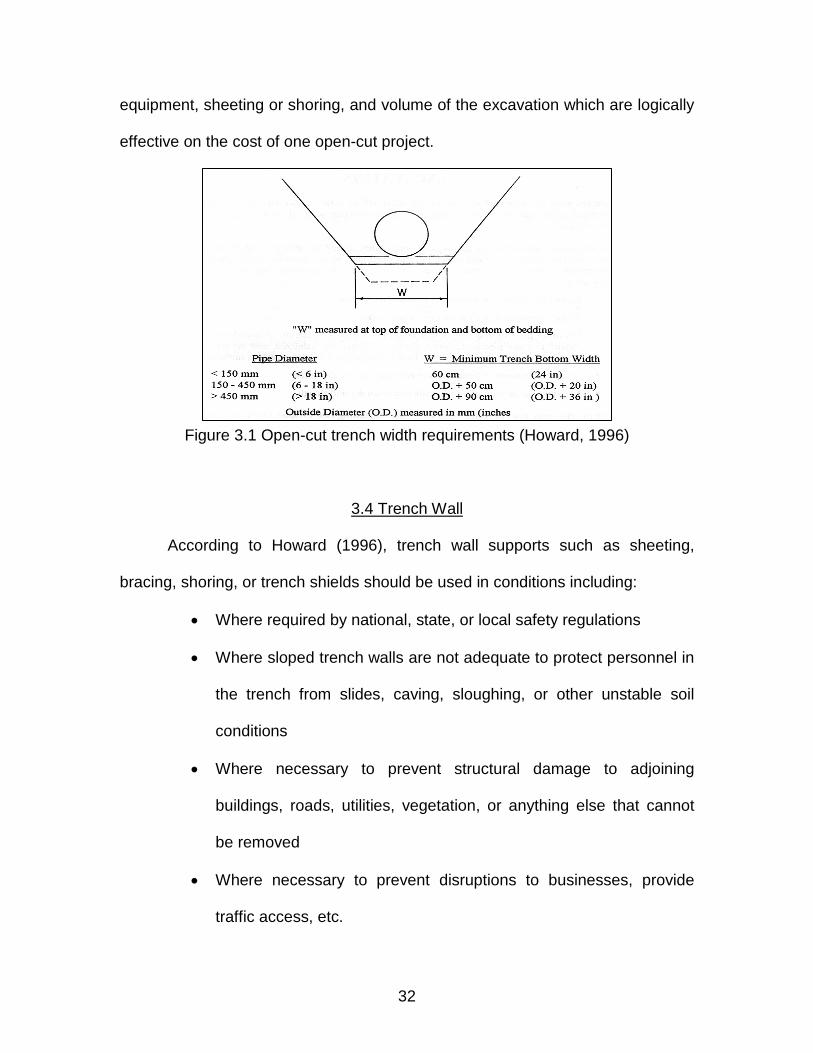
outside diameter (OD), construction methods, and inspection requirements.

Figure 3-1 shows a typical specification required width for trench. There are

some design assumptions as certain trench width at the top or bottom regarding

to the specification of the project. There are some successors based on the

design condition of the trench such as amount of dewatering time and

32

equipment, sheeting or shoring, and volume of the excavation which are logically

effective on the cost of one open-cut project.

Figure 3.1 Open-cut trench width requirements (Howard, 1996)

3.4 Trench Wall

According to Howard (1996), trench wall supports such as sheeting,

bracing, shoring, or trench shields should be used in conditions including:

• Where required by national, state, or local safety regulations

• Where sloped trench walls are not adequate to protect personnel in

the trench from slides, caving, sloughing, or other unstable soil

conditions

• Where necessary to prevent structural damage to adjoining

buildings, roads, utilities, vegetation, or anything else that cannot

be removed

• Where necessary to prevent disruptions to businesses, provide

traffic access, etc.

33

• Where necessary to remain within the construction easement of

right-of-way

Basically, there are two main types of trench walls, vertical and sloping so

that each one includes specific cost parameter characteristics and is related to

the type of pipe material, soil, and project conditions. Figure 3-2 shows a

schematic view of trench wall.

a) b)

Figure 3.2 Site clearances for trench walls. a) Vertical trench wall and b) Sloping trench wall. O.D. is outside pipe diameter. Retrieved from Howard (2004)

3.5 Bedding and Laying

The bedding is the material placed on the bottom of the trench to provide

uniform support for the pipe. Consistent support is essential to support the pipe

longitudinally, as well as to spread out the load on the underside of the pipe. The

34

bedding is placed in a way that the pipe will be at the appropriate elevation and

slope when the pipe is laid on the bedding. The thickness of the bedding also

varies depending on the type and size of pipe. Typically the minimum bedding

thickness is 4 to 6 inches (Howard, 1996).

3.6 Embedment

The embedment is the material placed around the pipe to act with the pipe

together as a pipe-soil structure to support the external loads on the pipe. Each

pipe-soil system has been selected or designed for the specific conditions of

pipeline. The embedment is designed to serve different functions for either rigid

or flexible pipe. The embedment for rigid pipe takes the load on the top of the

pipe such as dead, live, or weight of the pipe and distribute the load to the soil on

the bottom of the pipe. While in the flexible pipe, the embedment gives the

resistance to the pipe deflecting (Howard, 1996).

.

3.7 Backfill and Compaction

Backfill is the material placed above the embedment soil and pipe which

depending on the height of the embedment, backfill may or may not be in contact

with the pipe. Usually the excavated material from the trench is used as backfill

with a few exceptions such as scalping off large rock particles.

When using a backfill material that will settle excessively, such as organic

materials, frozen soil, and loosely-placed large mass of soil, the ground surface

35

should be mounted over the trench, or other provisions should be made to

prevent a depression over the pipe (Howard, 1996).

Figure 3.3 Open-cut trench cross section view (Howard, 1996)

As Figure 3.3 shows, there are various steps in open-cut technique from

excavation of the trench all the way to the compaction of the trench either in

installing new underground pipeline or replacing the deteriorated or under–

capacity size existing utility which each one of these operation consume the

project budget.

3.8 Summary

This chapter covered the construction steps necessary for open-cut

method. These steps include trench excavation, trench walls, bedding and laying,

embedment, backfill, and compaction.

36

CHAPTER 4

COST ANALYSIS OF OPEN-CUT AND PIPE BURSTING

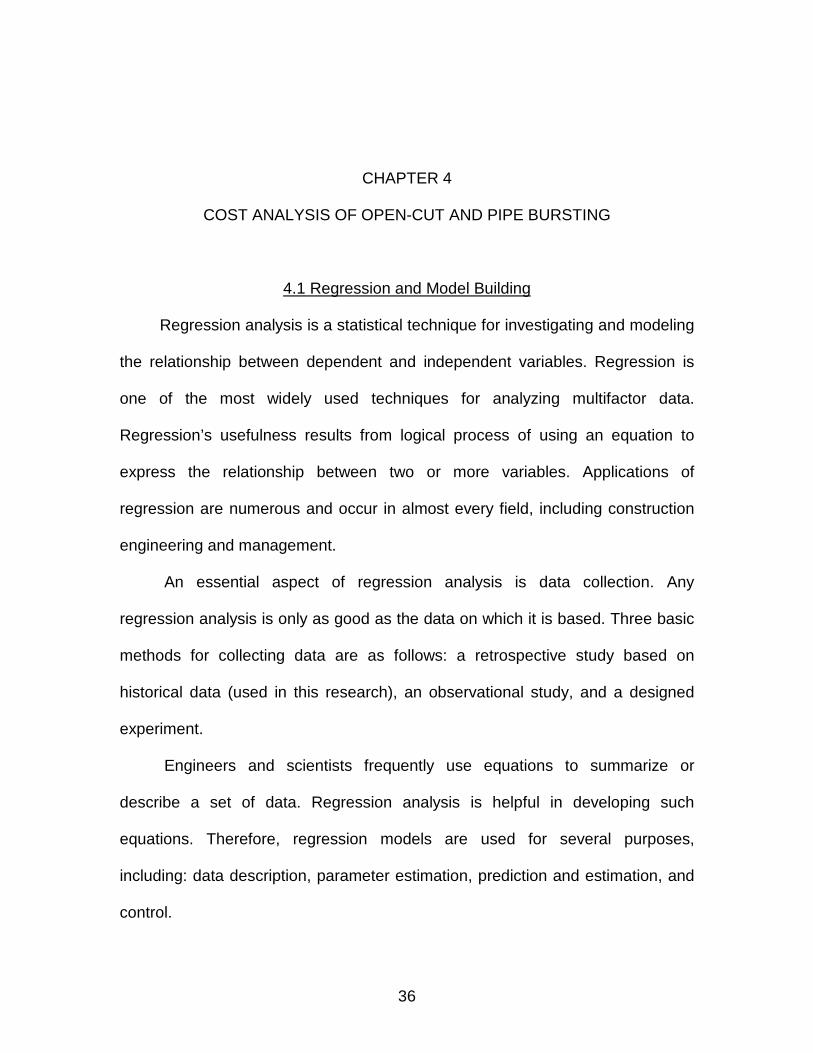
4.1 Regression and Model Building

Regression analysis is a statistical technique for investigating and modeling

the relationship between dependent and independent variables. Regression is

one of the most widely used techniques for analyzing multifactor data.

Regression’s usefulness results from logical process of using an equation to

express the relationship between two or more variables. Applications of

regression are numerous and occur in almost every field, including construction

engineering and management.

An essential aspect of regression analysis is data collection. Any

regression analysis is only as good as the data on which it is based. Three basic

methods for collecting data are as follows: a retrospective study based on

historical data (used in this research), an observational study, and a designed

experiment.

Engineers and scientists frequently use equations to summarize or

describe a set of data. Regression analysis is helpful in developing such

equations. Therefore, regression models are used for several purposes,

including: data description, parameter estimation, prediction and estimation, and

control.

37

4.1.1 Simple Regression Model

According to Montgomery and et al. (2006), simple regression is a model

with a single independent variable or regressor (x) that has a relationship with a

response (y) through a straight line. Eq. 4.1 shows the simple linear regression

model equation.

0 1y xβ β ε= + + Eq. 4.1

where the intercept 0β and the slope 1β are unknown constants and ε is a

random error component. The parameters 0β and 1β are estimated using sample

data and the Least Squares Regression method. The 0β and 1β estimation

process involves summing the squares of the differences between the

observation data and a single estimate of the measure of central tendency—the

mean—is minimum. The formulas and calculation process of the simple linear

regression method are provided in appendix A.

4.1.2 Multiple Regression Model

A regression model that involves more than one independent variable

(regressor) is called a multiple regression model. In general, the response y may

be related to k regressor or predictor variables. Eq. 4.2 shows the multiple linear

regression model with k variables:

0 1 1 2 2 ...β β β β ε= + + + + +k ky x x x Eq. 4.2

38

The parameters jβ , j=0, 1,…, k, are called the regression coefficients. The

parameter jβ represent the expected change in the response y per unit change in

jx when all of the remaining regressor variables ix ( i j≠ ) are held constant. The

formulas and calculation process of the multiple linear regression method is

provided in appendix B.

4.2 Pipe Bursting

4.2.1 Data Collection

As mentioned previously, the considered methodology in this research is

based on statistical techniques for analyzing the gathered data from surveys and

TCC data base. To collect the data, a survey of companies and water and sewer

departments of municipalities was conducted. Additionally, a database published

by the Trenchless Technology Center (TTC) at Louisiana Tech University was

used. TTC data for various pipe bursting projects is included in Appendix C. The

raw survey results and the survey questionnaire are included in Appendix E and

Appendix D. Table 4.1 presents a summary of all collected data.

39

Table 4.1 Pipe Bursting Data

Location Year Name of Project Length

(ft) Diameter

(in.) Price ($/ft)

Ratio 2007 Price ($/ft)

Fort Wayne, IN

2000 Sunny Meadows Sanitary Sewer Rehabilitation

2,637 12 112 1.37 154

Greeley, CO 2001 Sewer Rehabilitation Project

678 6 81 1.33 108

Libertyville, IL 2000 Wildwood 15 in. Interceptor Upgrade

88 15 161 1.37 220

San Antonio, TX

2000 Briarcroft Emergency Sewer Rehab Project

175 8 112 1.37 154

San Antonio, TX

2001 Westlyn Sanitary Sewer Emergency Rehab

1,112 8 103 1.33 137

San Antonio, TX

2002 Pipe Bursting Construction Contract

3,000 10 46 1.29 59

San Antonio, TX


1,000 12 70 1.29 91

San Antonio, TX


1,000 18 128 1.29 164

San Antonio, TX

2002 Pipe Bursting Construction

1,000 21 54 1.29 70

San Diego, CA 2002 Sewer Group Job 510 8 100 1.29 129

Berkeley, CA 2002 Sanitary Sewer Rehab. and Replacement

1,690 6 70 1.29 90

Berkeley, CA 2002 Sanitary Sewer Rehab. and Replacement

3,620 6 70 1.29 90

Boston, MA 2000 Sewer and Waterworks Improvements

910 10 80 1.37 110


910 15 100 1.37 137

Boston, MA 2000 Sewer/waterworks Improvements

790 18 130 1.37 178

40

Table 4.1 - Continued


944 12 150 1.37 206

Lancing, MI 2004 Pipe Bursting Construction Contract

310 18 168 1.16 194

Dallas, TX 2000 Lower Five Mile Creek

650 8 138 1.37 189


500 18 91 1.37 125


600 21 105 1.37 144

Dallas, TX 2000 Replacement in IH 635,75,35,45E

120 6 66 1.37 91

Dallas, TX 2000 Replacement in IH 635,75,35,45E

80 8 85 1.37 116

Dallas, TX 2001 Misc. Water and Wastewater Replacement

1,550 12 71 1.33 95

Burleson, TX 2007 Elk Ridge Relief Sewer

4,500 12 100 1 100

Dallas, TX 2008 Dallas Water Utilities Contract #08-003/004

770 6 55 0.97 54

Garland, TX 2008 Leon Pipe Burst 1,590 8 60 0.97 59

Pocatello, ID 2008 Downtown Sanitary Sewer Rehab Phases II and III

700 8 105 0.97 102

Pine Bluff, AR 2006 2006 Pipe Bursting Project

3,596 6 58 1.04 60

Troy, MI 2008 City of Troy Water Main replacement

2,000 6 50 0.97 59

San Francisco, CA

2008 Pipe Bursting Project

3,000 12 65 0.97 63

Table 4.1 includes the location, year, name of the project, length (ft),

diameter (inch), and the total price of the project (dollar per foot). Since there are

projects in different years and base year for doing the analysis assumed to be

2007; therefore, all the other years’ prices have been multiplied by the year-to-

year ratio to become compatible with 2007 prices. These conversion ratios are

retrieved from R.S. Means database.

41

0

50

100

150

200

250

5 10 15 20 25

Diameter (in.)

Pric

e ($

/ft)

0

50

100

150

200

250

0 1000 2000 3000 4000 5000

Length (ft)

Pric

e ($

/ft)

4.2.2 Pipe Bursting Data Analysis

After collecting data, we analyzed the data with regression method. In this

research, there is one intercept parameter and two main variables that would be

analyzed based on price per foot of pipe bursting as intercept parameter and

length and diameter of pipeline project as variables.

As Figure 4.1 (a) illustrates, each project data has been divided in the

form of price (dollar per foot) versus diameter (inch), or in the form of price (dollar

per foot) versus length of project (foot) as shown in Figure 4.1 (b).

(a)

(b)

Figure 4.1 Scatter plots of pipe bursting data (a) Cost versus pipe diameter size and (b) cost versus length of project.

42

0

50

100

150

200

250

5 10 15 20 25

Diameter (in.)

Pric

e ($

/ft)

0

50

100

150

200

250

5 10 15 20 25

Diameter (in.)

Pric

e ($

/ft)

0

50

100

150

200

250

5 10 15 20 25

Diameter (in.)

Pric

e ($

/ft)

0

50

100

150

200

250

5 10 15 20 25

Diameter (in.)

Pric

e (

$/ft)

Now that the scatter plot and graphs are ready, finding a proper and

significant trend equation based on relationship between these variables would

be the next step. Therefore, regression technique of the statistical methods

would be a good tool. As there are different regression methods, such as straight

linear, exponential, logarithmic, and power, it is important to decide the best fit

trend line on the scatter plot. Relationship ratio between two parameters, R-

squared (R2), would be a proper decision criteria. Obviously, the higher the R2,

the more accurate the trend line will be.

(a) (b)

(c) (d)

Figure 4.2 Fit trend line on pipe bursting cost and diameter data (a) linear (b) logarithmic (c) power (d) exponential regression.

43

Figure 4.2 shows four different regression trend lines fitted on the cost-

diameter size data regarding to pipe bursting projects. As mentioned before, to

find out the best fitted trend line on these data, the relationship between variables

(R2) would be the criteria, so that the higher (R2) the higher relationship between

the cost and variables. Table 4.2 shows each line equation and the related R2 of

that line. As third column shows, the highest relationship ratio with regards to

logarithmic regression with equation of y= 52.385Ln(x) - 3.3132 and R2 of 0.21.

Parameter “y” and “x” respectively are cost and diameter size, respectively.

Table 4.2 Cost vs. Diameter, Trend Lines Comparison

Regression Type Equation R Square (R2)

Linear y = 4.2342x + 71.218 0.18

Logarithmic y = 52.385Ln(x) - 3.3132 0.21

Power y = 38.364 x 0.4497 0.20

Exponential y = 72.846e 0.0362x 0.17

The same process would be performed to figure out the relationship

between cost and length of the pipe bursting from collected data. Figure 4.3

similarly shows four different regression lines fitted on the data and Table 4.3

shows each line equation and the related R2 of that line. As third column shows,

the highest relationship ratio regards to power regression with equation of y=

52.385Ln(x) - 3.3132 and R2 of 0.24. Parameter “y” and “x” respectively are cost

($/ft) and length size (ft) of the project, respectively.

44

0

50

100

150

200

250

0 1000 2000 3000 4000 5000

Length (ft)

Pri

ce (

$/ft

)

0

50

100

150

200

250

0 1000 2000 3000 4000 5000

Length (ft)

Pri

ce (

$/ft

)

0

50

100

150

200

250

0 1000 2000 3000 4000 5000

Length (ft)

Pric

e ($

/ft)

0

50

100

150

200

250

0 1000 2000 3000 4000 5000

Length (ft)

Pric

e ($

/ft)

(a) (b)

(c) (d)

Figure 4.3 Fit trend line on pipe bursting cost and length data (a) linear (b) logarithmic (c) power (d) exponential regression

Table 4.3 Cost vs. Length, Trend Lines Comparison


Linear y = -0.0193x + 144.12 0.223

Logarithmic y = -21.767Ln(x) + 265.59 0.230

Power y = 400.23x -0.1923 0.236

Exponential y = 137.29e-0.0002x 0.235

45

The statistical Analysis System software known as SAS is one the most

powerful software for statistical analysis. In this research SAS is used to analyze

and find out the mathematical relationship between the problem’s variables. The

starting step with this software would be inserting the codes for the particular

program. Appendix G shows the codes that have been used in this research.

After inserting the codes and the gathered data, it is time to run the

program and calculate the results. The way that SAS will solve the multiple

variable regression, is the matrix technique which is demonstrated in appendixes

A and B. Appendix H shows the data matrix of the program and appendix I

demonstrates how SAS solve the program by using matrix method.

Figure 4.4 shows the scattered plot of the data which is used as input in

SAS software. The perpendicular axes in all four graphs in Figure 4.4 is cost

parameter that is in dollar per foot format and respectively horizontal axes are

diameter size (inch), length of project (foot), L2 (length square), LD (logarithm of

diameter), and LL (logarithm of length) parameters. Each graph shows the points

related to the amount of the two variables of the inserted data. For example, the

cost-diameter graph indicates how the data is scattered regarding to cost and

diameter amounts of data. The “L2” variable is defined as square of the length of

each data and “LD” variable is defined as logarithm of the diameter size and “LL”

variable is defined as logarithm of the length size. These three variables have

been added to the programs regarding to the single regression equations of the

cost-diameter and cost-length for more accuracy of the model.

46

(a) (b)

(c) (d)

(e)

Figure 4.4 SAS scattered plot of pipe bursting data. (a) cost vs. diameter size (b) cost vs. length (c) cost vs. length square (d) cost vs. logarithm of diameter

(e) cost vs. logarithm of length.

47

The fit Analysis option of SAS has the ability to run the model with

different variables to determine which combination of variables would be the best

estimation of the data. During this process, four combinations have been

considered for comparison; the first combination includes the main simple

variables; diameter and length as shown in Figure 4.5.

Figure 4.5 Fit Analysis of the length and diameter variables

48

As Figure 4.5 shows, the R2 of this regression line is 0.29. Second

combination includes the main simple variables; diameter and length and

additional L2 that is shown in Figure 4.6. As Figure 4.6 shows, the R2 of this

regression line is 0.34 and it indicates that the second combination is more

accurate than the first combination.

Figure 4.6 Fit Analysis of the length, diameter, and L2 variables

49

The third combination of variables includes the LD, L2, and length

variables. The Fit analysis of SAS for this combination is shown in Figure 4.7.

Regarding Figure 4.7, the R2 of this regression line is 0.38, which it indicates that

the third combination is more accurate than the first two combinations.

Figure 4.7 Fit Analysis of the length, L2, and LD variables

50

Finally Figure 4.8 shows the Fit Analysis of the best combination of

variables, namely are diameter, length, L2, LD, and LL. The amount of the R2 for

this combination is 0.48. Consequently the fourth combination would be the

selected regression equation fitted on the pipe bursting data.

Figure 1

Figure 4.8 Fit Analysis of the length, diameter, L2, LD, and LL variables

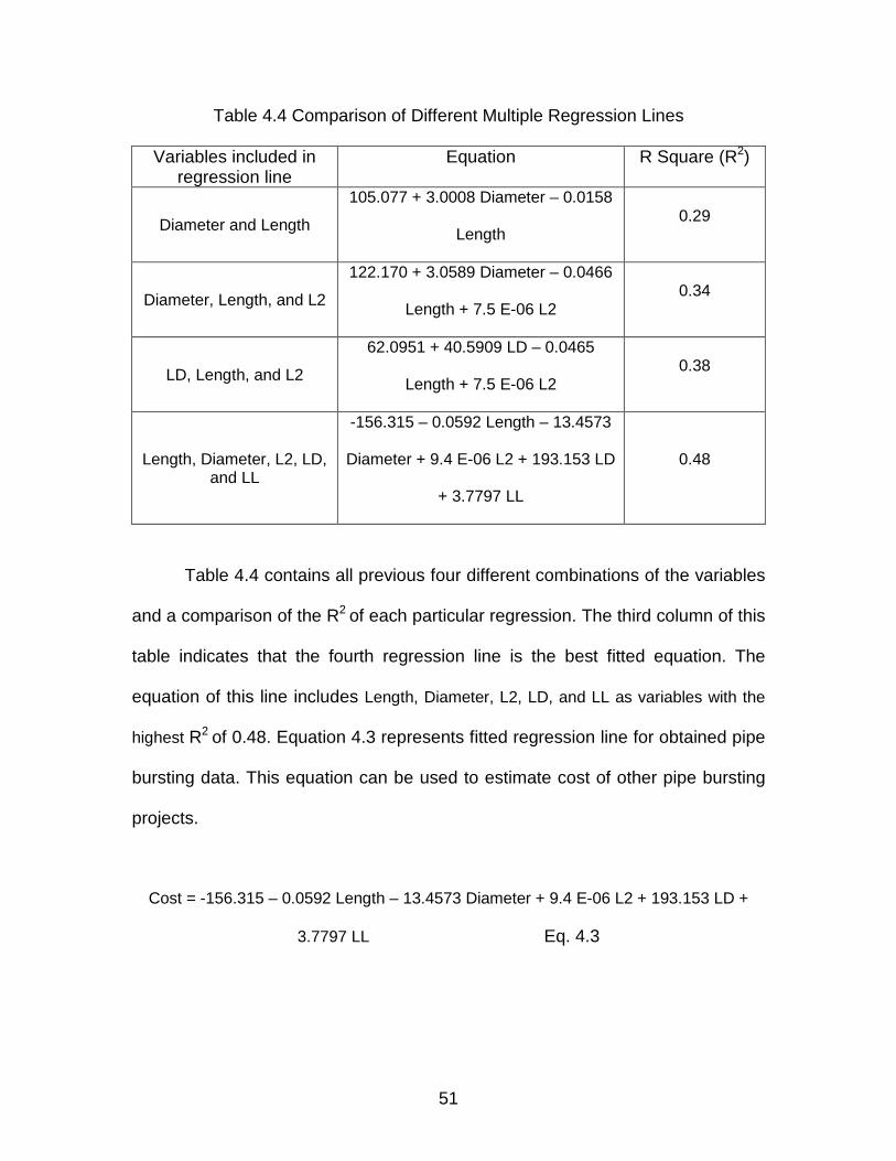
51

Table 4.4 Comparison of Different Multiple Regression Lines

Variables included in regression line

Equation R Square (R2)

Diameter and Length

105.077 + 3.0008 Diameter – 0.0158

Length 0.29

Diameter, Length, and L2

122.170 + 3.0589 Diameter – 0.0466

Length + 7.5 E-06 L2 0.34

LD, Length, and L2

62.0951 + 40.5909 LD – 0.0465

Length + 7.5 E-06 L2 0.38

Length, Diameter, L2, LD, and LL

-156.315 – 0.0592 Length – 13.4573

Diameter + 9.4 E-06 L2 + 193.153 LD

+ 3.7797 LL

0.48

Table 4.4 contains all previous four different combinations of the variables

and a comparison of the R2 of each particular regression. The third column of this

table indicates that the fourth regression line is the best fitted equation. The

equation of this line includes Length, Diameter, L2, LD, and LL as variables with the

highest R2 of 0.48. Equation 4.3 represents fitted regression line for obtained pipe

bursting data. This equation can be used to estimate cost of other pipe bursting

projects.

Cost = -156.315 – 0.0592 Length – 13.4573 Diameter + 9.4 E-06 L2 + 193.153 LD +

3.7797 LL Eq. 4.3

52

4.3 Open-Cut

4.3.1 Data Collection

Similar to the pipe bursting data analysis, the considered methodology to

analyze the open-cut data is also based on the statistical techniques. The data of

open-cut projects have been gathered from the survey of “Construction Cost

Comparison of Open-Cut and Pipe Bursting for Municipal Water, Sewer and Gas

Applications.” The questionnaire of the mentioned survey is attached in appendix

E and the complete details of the gathered data are shown in appendix D. Table

4.5 includes all the collected data from the open-cut projects based on the

conducted survey.

Table 4.5 Open-Cut Data

Location Year Name of Project Length

(ft) Diameter

(in.) Price ($/ft)

Ratio 2007 Price ($/ft)

Cambridge, MS

2006 Sanitary sewer & storm drain

220 8 417 1.04 434

Cambridge, MS

2006 Sanitary sewer &

storm drain 220 12 625 1.04 650

Dallas, TX 2008 Dallas Water

Utilities Contract #08-003/004

915 6 90 0.97 87

Greeley, CO 2008

2008 Sanitary Sewer

Rehabilitation Projects

1,729 6 221 0.97 214

Garland, TX 2008 Sasche Relief Line & metering Station

2,050 24 217 0.97 210

Chattanooga, TN

2008 Charger Drive replacement

158 8 190 0.97 184

Pine Bluff, AR 2005 Pennsylvania

Street Re-Construct.

214 6 47 1.07 50

Santa Ramon, CA 2008

Ollinger Canyon Road 7,000 16 225 0.97 218

San Francisco, CA

2008 San Francisco Airport Project

10,000 12 120 0.97 116

53

Table 4.5 includes the location, year, name of the project, length (foot),

diameter (inch), and the price of the project (dollar per foot) as main information

of the each project. Since there are projects in different years and the base year

for preparing the analysis is assumed to be 2007; therefore, all the other years’

prices have been multiplied by the year-to-year ratio to become compatible with

2007 dollars. These conversion ratios are retrieved from R.S. Means (2007)

database.

4.3.2 Open-Cut Data Analysis

While due to limited time and resources, we did not obtain sufficient open-

cut cost data, nevertheless, only for comparison purposes we continued our

regression analysis for the limited data we collected. As mentioned previously, in

this research there is one intercept parameter and two main variables that would

be analyzed based on; price of per foot of open-cut as intercept parameter,

length and diameter size of pipeline project as variables.

As Figure 4.9 demonstrates, each project data has been graphed in the

form of price (dollar per foot) versus Diameter size (inch) in Figure 4.9 (a), or in

the form of price (dollar per foot) versus Length of project (foot) in Figure 4.9 (b).

54

(a)

(b)

Figure 4.9 Scatter plots of open-cut data. (a) Cost versus pipe diameter size (b) cost versus length of project.

Now that the scatter plot data and graphs are ready, finding a proper and

significant trend equation based on the relationship between these variables

would be next step and the regression technique would be a good tool. As there

are different regression methods, such as straight linear, exponential,

logarithmic, and power, it is important to decide the best fit trend line on the

scatter plot. Relationship ratio between two parameters, R-squared (R2), would

0

100

200

300

400

500

600

700

0 2000 4000 6000 8000 10000 12000

Length (ft)

Pri

ce (

$/ft

)

0

100

200

300

400

500

600

700

5 10 15 20 25

Diameter (in.)

Pric

e ($

/ft)

55

0

100

200

300

400

500

600

700

5 10 15 20 25

Diameter (in.)

Pric

e ($

/ft)

0

100

200

300

400

500

600

700

5 10 15 20 25

Diameter (in.)

Pric

e ($

/ft)

0

100

200

300

400

500

600

700

5 10 15 20 25

Diameter (in.)

Pric

e ($

/ft)

0

100

200

300

400

500

600

700

5 10 15 20 25

Diameter (in.)

Pric

e ($

/ft)

be a proper decision criterion, with the higher the R2, the more accuracy of the

trend line.

(a) (b)

(c) (d)

Figure 4.10 Fit trend line on cost and diameter size of open-cut data. (a) linear (b) logarithmic (c) power (d) exponential regression.

Figure 4.10 shows four different regression trend lines fitted on the cost-

diameter size data for the open-cut projects. As mentioned before, to find out the

best fitted trend line on these data, relationship ratio between variables (R2)

56

would be the criteria. Table 4.6 shows each line equation and the related R2 of

that line. As the third column shows, the highest relationship ratio is for the power

regression with equation of y = 49.537x0.5812 and R2 of 0.13. Variables “y” and “x”

respectively would be cost and diameter size.

Table 4.6 Cost vs. Diameter, Trend Lines Comparison


Linear y = 4.226x + 194.55 0.02

Logarithmic y = 89.992Ln(x) + 36.035 0.05

Power y = 49.537x0.5812 0.13

Exponential y = 125.95e0.0356x 0.08

Same process would be performed to figure out the relationship between

cost and length of the pipe bursting collected data. Figure 4.11 similarly shows

four different regression lines fitted on the data and Table 4.7 shows each line

equation and the related R2 of that line. As the third column shows, the highest

relationship ratio is achieved for the Logarithmic regression with the equation

y = -42.976Ln(x) + 532.7 and R2 of 0.1306. Variables “y” and “x” respectively would

be cost ($/ft) and length size (ft) of the project.

57

0

100

200

300

400

500

600

700

0 5000 10000 15000

Length (ft)

Pric

e ($

/ft)

0

100

200

300

400

500

600

700

0 5000 10000 15000

Length (ft)

Pric

e ($

/ft)

0

100

200

300

400

500

600

700

0 5000 10000 15000

Length (ft)

Pri

ce (

$/ft)

0

100

200

300

400

500

600

700

0 5000 10000 15000

Length (ft)

Pri

ce (

$/ft)

(a) (b)

(c) (d)

Figure 4.11 Fit trend line on cost and length of open-cut data. (a) linear (b) logarithmic (c) power (d) exponential regression.

Table 4.7 Cost vs. Length, Trend Lines Comparison


Linear y = -0.0155x + 279.27 0.0848

Logarithmic y = -42.976Ln(x) + 532.7 0.1306

Power y = 326.89x-0.0833 0.028

Exponential y = 202.59e-4E-05x 0.0255

58

In this part of the research, one more time SAS is used to analyze and

find out the mathematical relationship among the variables. The starting step with

this software would be inserting the codes for the particular program. Appendix J

shows the codes have been used in this research for SAS.

After inserting the codes and the gathered data, it is time to run the

program. The way that SAS will solve the multiple variable regression is the

matrix technique, demonstrated in appendix A and B. Appendix K shows the data

matrix of the program and appendix I demonstrates how SAS solves the program

by using the matrix method.

Following Figure 4.12 shows the scattered plot of the data which is input in

the SAS software. The perpendicular axes in all four graphs in Figure 4.12 is the

cost variable that is in dollars per foot unit and respectively horizontal axes are

diameter size (inch), length of project (foot), L2 (length square), LD (logarithm of

diameter), and LL (logarithm of length) parameters. Each graph shows the points

related to the value of the two variables of the inserted data. For example, the

cost-diameter graph indicates how the data is scattered regarding the cost and

diameter amounts of the data. The “L2” variable is defined as the square of the

length of each data and “LD” parameter is defined as the logarithm of the

diameter size and the “LL” variable is defined as logarithm of the length size.

These three variables have been added to the programs regarding to the single

regression equations of the cost-diameter and cost-length for more accuracy of

the model.

59

(a) (b)

(c) (d)

(e)

Figure 4.12 SAS scattered plot of open-cut data. (a) cost vs. diameter size (b) cost vs. length (c) cost vs. length square (d) cost vs. logarithm of diameter

(e) cost vs. logarithm of length.

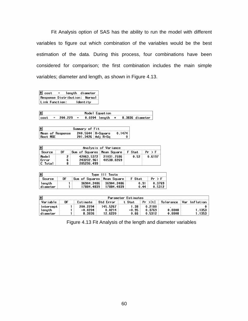
60

Fit Analysis option of SAS has the ability to run the model with different

variables to figure out which combination of the variables would be the best

estimation of the data. During this process, four combinations have been

considered for comparison; the first combination includes the main simple

variables; diameter and length, as shown in Figure 4.13.

Figure 4.13 Fit Analysis of the length and diameter variables

61

As Figure 4.13 shows, the R2 of this regression line is 0.15. The second

combination includes the length and additional LD as illustrated in Figure 4.14.

As Figure 4.14 shows, the R2 of this regression line is 0.25 which indicates that

the second combination is more accurate than the first.

Figure 4.14 Fit Analysis of the length and LD variables

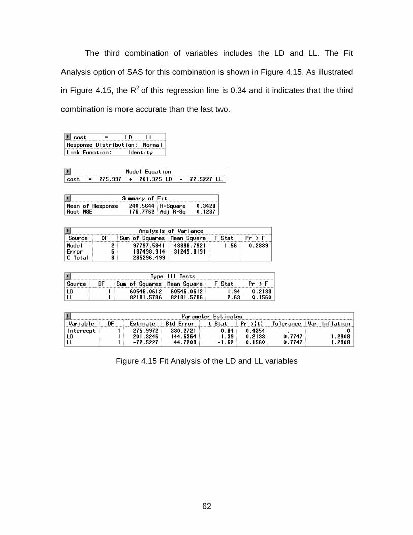
62

The third combination of variables includes the LD and LL. The Fit

Analysis option of SAS for this combination is shown in Figure 4.15. As illustrated

in Figure 4.15, the R2 of this regression line is 0.34 and it indicates that the third

combination is more accurate than the last two.

Figure 4.15 Fit Analysis of the LD and LL variables

63

Finally, Figure 4.16 shows the Fit Analysis option of SAS for combination

of variables namely the diameter, length, L2, LD, and LL. The amount of the R2

for this combination is 0.88. Consequently, the fourth combination would be the

selected regression equation fitted on the pipe bursting data.

Figure 4.16 Fit Analysis of the LD and LL variables

64

Table 4.8 Comparison of Different Multiple Regression Lines

Variables included in regression line

Equation R Square (R2)

Diameter and Length

200.229 – 0.0204 Length + 8.3836

Diameter 0.15

Length and LD

-84.1502 + 171.249 LD – 0.0258

Length 0.25

LD and LL 275.997 + 201.325 LD – 72.5227 LL 0.34

Length, Diameter, L2, LD, and LL

-4701.98 – 0.2507 Length – 193.836

Diameter + 1.0 E-05 L2 + 2576.18 LD

+ 242.461 LL

0.88

Table 4.8 includes all previous four different combinations of the

parameters and compares the R2 of each particular regression. The third column

of this table indicates that the fourth regression line is the best fitted equation.

The equation of this line includes Length, Diameter, L2, LD, and LL as variables with

the highest R2 amount of 0.88. Therefore, to estimate similar open-cut projects,

the regression line is:

Cost = - 4701.98 – 0.2507 Length – 19.836 Diameter + 1.0 E-05 L2 + 2576.18 LD +

242.461 LL Eq. 4.4

65

0

100

200

300

400

500

600

700

5 10 15 20 25

Diameter (in.)

Pric

e ($

/ft)

0

100

200

300

400

500

600

700

5 10 15 20 25

Diameter (in.)

Pric

e ($

/ft)

0

100

200

300

400

500

600

700

0 5000 10000 15000

Length (ft)

Pric

e ($

/ft)

0

100

200

300

400

500

600

700

0 1000 2000 3000 4000 5000

Length (ft)

Pric

e ($

/ft)

4.4 Comparison

After identifying the most fitted trend lines over the data of both pipe

bursting and open-cut and attaining their regression equations, pipe bursting

proves to be less expensive compare to the open-cut method, as shown in

Figure 4.17.

Open-cut Pipe Bursting

(a) (b)

(c) (d)

Figure 4.17 Comparison of trend lines of open-cut and pipe bursting. (a) open-cut price vs. diameter (b) pipe bursting price vs. diameter (c) open-cut

price vs. length (d) pipe bursting price vs. length

66

Figure 4.17 (c) and (d) point out that the relationship between length

versus the cost in both pipe bursting and open-cut methods. There is an inverse

relationship between the length of the project and the cost of project. However;

there is a sharp decrease at the beginning of the project and then relationship

becomes flat in longer lengths. Overall, considering length of project shown in

Figures 4.17 (c and d), pipe bursting is more cost effective that open-cut method.

According to Figure 4.17 (a) and (b), as far as the comparison is based on

the diameter size, until 25-inch size both methods demonstrate that the cost

steadily increase but the ratio of increasing the cost versus the diameter size in

open-cut is a little more than pipe bursting. However; approximately the total cost

of pipe bursting, considering diameter, is up to 40% less than open-cut.

4.5 Hypothesis Test

Statistically, hypothesis test is a proper way to prove that the average

price of pipe bursting is less than open-cut. For this test, standard deviation and

average price for both pipe bursting and open-cut cost data are necessary.

Tables 4.9 and 4.10 show the average and standard deviation with generic form

of price per-inch-per foot for both methods. By dividing the total cost of each

project (cost per foot multiply by length) over the product of diameter and length,

will arrive at the cost per-inch-per-foot of each project. If we divide the sum of

the cost per-inch-per-foot over the number of projects, we will obtain the average

cost. The standard deviation formula would be ( 2( )

1

x x

n

−

−∑ ).

67

Table 4.9 Average and Standard Deviation for Pipe Bursting Data

Project Length (ft)

Diameter (in.)

2007 Price ($/ft)

Diameter X Length

Total Cost ($) $/in./ft

1 2,637 12 154 31,644 $406,098 $12.83

2 678 6 108 4,068 $73,224 $18.00

3 88 15 220 1,320 $19,360 $14.67

4 175 8 154 1,400 $26,950 $19.25

5 1,112 8 137 8,896 $152,344 $17.13

6 3,000 10 59 30,000 $177,000 $5.90

7 1,000 12 91 12,000 $91,000 $7.58

8 1,000 18 164 18,000 $164,000 $9.11

9 1,000 21 70 21,000 $70,000 $3.33

10 510 8 129 4,080 $65,790 $16.13

11 1,690 6 90 10,140 $152,100 $15.00

12 3,620 6 90 21,720 $325,800 $15.00

13 910 10 110 9,100 $100,100 $11.00

14 910 15 137 13,650 $124,670 $9.13

15 790 18 178 14,220 $140,620 $9.89

16 944 12 206 11,328 $194,464 $17.17

17 310 18 194 5,580 $60,140 $10.78

18 650 8 189 5,200 $122,850 $23.63

19 500 18 125 9,000 $62,500 $6.94

20 600 21 144 12,600 $86,400 $6.86

21 120 6 91 720 $10,920 $15.17

22 80 8 116 640 $9,280 $14.50

23 1,550 12 95 18,600 $147,250 $7.92

24 4,500 12 100 54,000 $450,000 $8.33

25 770 6 54 4,620 $41,580 $9.00

26 1,590 8 59 12,720 $93,810 $7.38

27 700 8 102 5,600 $71,400 $12.75

28 3,596 6 60 21,576 $215,760 $10.00

29 2,000 6 59 12,000 $118,000 $9.83

30 3,000 12 63 36,000 $189,000 $5.25

Average $11.65 Standard Deviation 4.9

68

Table 4.10 Average and Standard Deviation for Open-Cut Data

Project Length (ft)

Diameter (in.)

2007 Price ($/ft)

Diameter X Length

Total Cost ($) $/in./ft

1 220 8 434 1,760 $95,480 $54.25

2 220 12 650 2,640 $143,000 $54.17

3 915 6 87 5,490 $79,605 $14.50

4 1,729 6 214 10,374 $370,006 $35.67

5 2,050 24 210 49,200 $430,500 $8.75

6 158 8 184 1,264 $29,072 $23.00

7 214 6 50 1,284 $10,700 $8.33

8 7,000 16 218 112,000 $1,526,000 $13.63

9 10,000 12 116 120,000 $1,160,000 $9.67

Average $24.66

Standard Deviation 18.84

The formula for one-sided hypothesis test for comparison of both methods’

mean would be:

2 21 2( 1) ( 1)

2PB OC

PB OC

n S n SS

n n− + −

′ =− −

and 1 1

( )

PB OCcalculation

PB OC

t

Sn n

µ µ−=

′ +

Where as 11.65PBµ = and 4.90PBS = are mean and standard deviation of

pipe bursting, respectively. Also, 24.66OCµ = and 18.84OCS = are mean and

standard deviation of open-cut, respectively. 30PBn = and 9OCn = are the

number of data for pipe bursting and open-cut, respectively. The hypothesis for

the comparison between the means of two methods is:

0

1

:

:PB OC

PB OC

H

H

µ µ

µ µ

=

⟨

Level of confidence for this test is assumed to be 95% ( 0.05α = ).

69

After plugging the available data into the formulas; we obtain 10.05S′ = and

consequently 3.40calculationt = − . Using “t” function standard table, the amount of t

for 0.05α = and the degree of freedom of 37 (30+9-2) would be 1.68.

Consequently, from statistical point of view, because 0.05,37calculationt t> we can

conclude that the 0H hypothesis would be rejected and 1H hypothesis would be

accepted. It means that with 95% of confidence, the average price of pipe

bursting would be less than open-cut method.

Next chapter concentrates on a case study to have a better understanding

of the cost comparison between open-cut and pipe bursting.

4.6 Summary

This chapter covered the data analysis of both pipe bursting and open-cut

methods. Excel and SAS software were used to develop the regression lines fit

on different combination of variables. Finally, a hypothesis test was performed to

verify results of regression analysis which indicated on the average pipe bursting

costs are less than traditional open-cut costs.

70

CHAPTER 5

CASE STUDY OF PIPE BURSTING VS. OPEN-CUT

5.1 Pipeline Infrastructure in City of Troy, Michigan

Previous chapters indicated that overall, cost bursting costs can be

expected to be less than open-cut costs. Several models and cost estimates

were developed to illustrate this fact. This chapter presents a hypothetical case

study, to show how U.S. municipalities would save millions of dollars if they use

innovative technologies such as pipe bursting. The case study presented here is

the replacement of the entire sewer system in the City of Troy in the State of

Michigan.

The City of Troy is located in Oakland County, Michigan. It is a suburb of

Detroit and considered a part of the Metro Detroit area. In the 2000 census, Troy

was the 12th largest city in Michigan by population, with 80,959 residents and

area of 33.6 square miles—33.5 square miles of land and 0.1 square miles of

lakes.

Figure 5.1 and 5.2 respectively show the location of the City of Troy and

the schematic layout of the sewer pipelines system.

71

Figure 5.1 Location of City of Troy in the State of Michigan

Figure 5.2 Sewer Pipeline Layout of City of Troy in the State of Michigan*

* Source: GIS Department, City of Troy

72

Table 5.1 shows the sewer system detail information which is retrieved

from the City of Troy GIS Department. In this table, the first column demonstrates

the 19 different diameter sizes (inch) and the second column consists of the

length size (feet) of each particular diameter size of the City of Troy sewer

pipeline. As it is obvious from the table, the total length of the sewer line would

be 2,051,370 feet and the diameter range is from 3 inches to 78 inches. It should

be noted that pipes with a diameter of 60 inches or more are challenging or and

not currently suitable for pipe bursting methods. Although they are presented

here for cost calculation purposes only, Simicevic and Sterling (2001) assert that

due to technology improvements, we will have up to 80 in. diameter pipe bursting

ability in the near future.

Table 5.1 City of Troy Sewer Pipeline Information

Pipe Diameter

(in.) Pipe Length

(ft) Pipe Diameter

(in.) Pipe Length

(ft) 3 1,900 27 13,737 6 7,810 30 11,140 8 1,194,414 36 22,256

10 219,310 42 2,767 12 431,924 48 11,563 15 81,958 60 10,859 17 319 66 1,397 20 71 72 1,900 21 20,857 78 1,178 24 16,010 TOTAL 2,051,370

73

5.2 Cost Estimating for Pipe Replacement Using Bursting Method

Now that we have the essential data, it is time to plug these information to

achieved regression equations from previous chapter and figure out what be the

cost of the city of Troy sewer system underground pipeline replacement using

pipe bursting technology. Table 5.2 demonstrates the summary calculation of the

City of Troy sewer system replacement cost by using the multiple regression

which is achieved in the previous chapter (Eq. 4.3). The equation for the cost of

pipe bursting considers Length, Diameter, L2 (Length square), LD (logarithm of

Diameter), and LL (logarithm of Length) as variables; Cost = -156.315 – 0.0592 Length –

13.4573 Diameter + 9.4 E-06 L2 + 193.153 LD + 3.7797 LL. Appendix M demonstrates

the detail calculations.

Table 5.2 Estimation of Pipe Bursting Cost by Multiple Regression

Diameter (in.) Length (ft.) Estimated Cost ($/ft) Total ($) 3 1,900 30 56,063 6 7,810 80 626,498 8 1,194,414 109 130,035,144 10 219,310 125 27,425,955 12 431,924 133 57,600,093 15 81,958 136 11,153,333 17 319 166 52,959 20 71 165 11,724 21 20,857 120 2,509,781 24 16,010 106 1,693,103 27 13,737 119 1,634,318 30 11,140 132 1,472,609 36 22,256 159 3,530,454 42 2,767 127 351,931 48 11,563 212 2,445,641

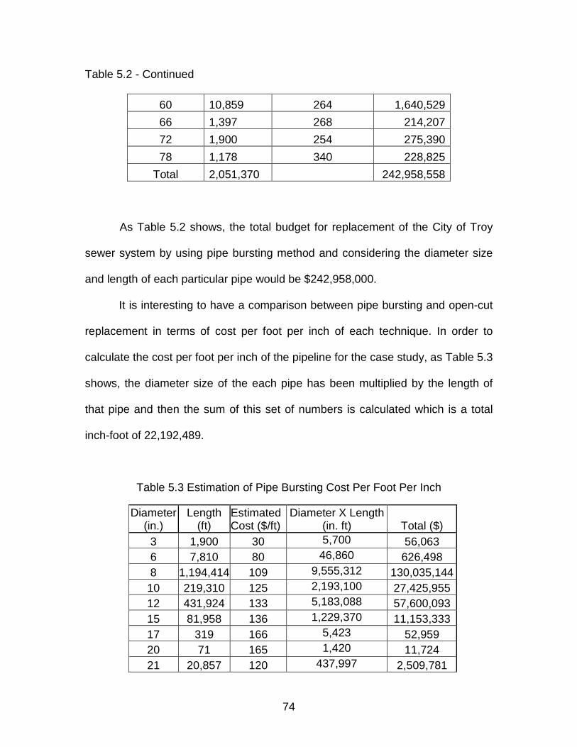
74


60 10,859 264 1,640,529

66 1,397 268 214,207

72 1,900 254 275,390

78 1,178 340 228,825

Total 2,051,370 242,958,558

As Table 5.2 shows, the total budget for replacement of the City of Troy

sewer system by using pipe bursting method and considering the diameter size

and length of each particular pipe would be $242,958,000.

It is interesting to have a comparison between pipe bursting and open-cut

replacement in terms of cost per foot per inch of each technique. In order to

calculate the cost per foot per inch of the pipeline for the case study, as Table 5.3

shows, the diameter size of the each pipe has been multiplied by the length of

that pipe and then the sum of this set of numbers is calculated which is a total

inch-foot of 22,192,489.

Table 5.3 Estimation of Pipe Bursting Cost Per Foot Per Inch

Diameter (in.)

Length (ft)

Estimated Cost ($/ft)

Diameter X Length (in. ft) Total ($)

3 1,900 30 5,700 56,063 6 7,810 80 46,860 626,498 8 1,194,414 109 9,555,312 130,035,144

10 219,310 125 2,193,100 27,425,955 12 431,924 133 5,183,088 57,600,093 15 81,958 136 1,229,370 11,153,333 17 319 166 5,423 52,959 20 71 165 1,420 11,724 21 20,857 120 437,997 2,509,781

75


Diameter (in.)

Length (ft)



24 16,010 106 384,240 1,693,103 27 13,737 119 370,899 1,634,318 30 11,140 132 334,200 1,472,609 36 22,256 159 801,216 3,530,454 42 2,767 127 116,214 351,931 48 11,563 212 555,024 2,445,641 60 10,859 264 651,540 2,866,776 66 1,397 268 92,202 214,207 72 1,900 254 136,800 275,390

78 1,178 340 91,884 228,825 Total 22,192,489 242,958,558

To calculate the cost of per-foot-per-inch of pipe bursting, the total amount

of pipe bursting cost ($242,958,000) would be divided by the total inch-foot

amount (22,192,489 in. ft) to arrive at the cost per-inch-per-foot of pipe bursting

as ≈$242,958,558

$11/in.ft.22,192,489 in. ft

76

5.3 Cost Estimating for Pipe Replacement Using Open-Cut Method

Similar to the pipe bursting cost estimation process for the City of Troy sewer

pipeline replacement, next step is to plug the information into the derived

regression equations from the previous chapter to figure out what the open-cut

cost would be. Table 5.4 demonstrates the summarized calculation of the City of

Troy sewer system replacement cost by using the multiple regression which is

obtained in the previous chapter (Eq. 4.4). The equation for cost of pipe bursting

considering Length, Diameter, L2 (Length square), LD (logarithm of Diameter), and LL

(logarithm of Length) as variables; Cost = - 4701.98 – 0.2507 Length – 19.836 Diameter

+ 1.0 E-05 L2 + 2576.18 LD + 242.461 LL. Appendix N demonstrates the details of

the calculation.

Table 5.4 Estimation of Open-Cut Cost by Multiple Regression

Diameter (in.) Length (ft) Estimated Cost ($/ft) Total ($) 3 1,900 70 133,326 6 7,810 140 1,096,080 8 1,194,414 166 198,134,675 10 219,310 189 41,417,906 12 431,924 210 90,689,536 15 81,958 239 19,591,392 17 319 257 82,008 20 71 283 20,061 21 20,857 291 6,062,551 24 16,010 314 5,029,210 27 13,737 353 4,854,594 30 11,140 393 4,374,251 36 22,256 471 10,486,893 42 2,767 550 1,521,093 48 11,563 628 7,264,555

77


60 10,859 785 8,527,826

66 1,397 864 1,206,806

72 1,900 942 1,790,537

78 1,178 1,021 1,202,644

Total 2,051,370 403,485,944

As Table 5.4 shows, the total budget for replacement of the City of Troy

sewer system by using open-cut method and considering the diameter size and

length of each particular pipe would be $403,486,000.

A proper comparison between pipe bursting and open-cut replacement

cost is to have the cost per foot per inch of each technique. In order to calculate

the cost per foot per inch of the pipeline for the case study, as Table 5.5 shows,

the diameter size of each pipe has been multiplied by the length of that pipe and

then the sum of this set of numbers is calculated to arrive at a total of 22,192,489

in. ft.

Table 5.5 Estimation of Open-Cut Cost Per Foot Per Inch

Diameter (in.)

Length (ft)



3 1,900 70 5,700 133,326 6 7,810 140 46,860 1,096,080 8 1,194,414 166 9,555,312 198,134,675

10 219,310 189 2,193,100 41,417,906 12 431,924 210 5,183,088 90,689,536 15 81,958 239 1,229,370 19,591,392 17 319 257 5,423 82,008 20 71 283 1,420 20,061 21 20,857 291 437,997 6,062,551

78


Diameter (in.)

Length (ft)



24 16,010 314 384,240 5,029,210 27 13,737 353 370,899 4,854,594 30 11,140 393 334,200 4,374,251 36 22,256 471 801,216 10,486,893 42 2,767 550 116,214 1,521,093 48 11,563 628 555,024 7,264,555 60 10,859 785 651,540 8,527,826 66 1,397 864 92,202 1,206,806 72 1,900 942 136,800 1,790,537 78 1,178 1,021 91,884 1,202,644

Total 22,192,489 403,485,944

To calculate the cost per-foot-per-inch of pipe bursting, the total amount of

open-cut cost ($403,486,000) would be divided over the total inch-foot amount

(22,192,489 in. ft) to obtain the cost per-inch-per-foot of pipe bursting as

≈$403,485,944

$18/in.ft22,192,489 in. ft

.

79

5.4 Cost Comparison Results and Analysis

Table 5.6 and Figure 5.3 show the estimated total cost for sewer pipeline

replacement in the City of Troy using the open-cut and pipe bursting methods.

For the traditional open-cut, the total cost was $403,486,000 while the estimated

cost using the pipe bursting technique was $242,959,000. Subtracting the pipe

bursting cost from the open-cut cost gives a savings of $160,527,386. With

respect of the cost of per-inch-per-foot of both methods, pipe bursting shows a

cost of $11 per-inch-per-foot while open-cut costs $18 per-inch-per-foot. Thus

pipe bursting cost approximately 40% less than the cost of open-cut. The

difference between two methods from point of view of cost per-inch-per-foot is

shown in Table 5.6, showing $7 less for pipe bursting per-inch-per-foot of pipe.

Figure 5.3 Estimated Sewer Pipeline Replacement Cost Comparison for

City of Troy

0

50

100

150

200

250

300

350

400

450

Open-Cut Pipe-Burst ing

Mill

ion

Dol

lar

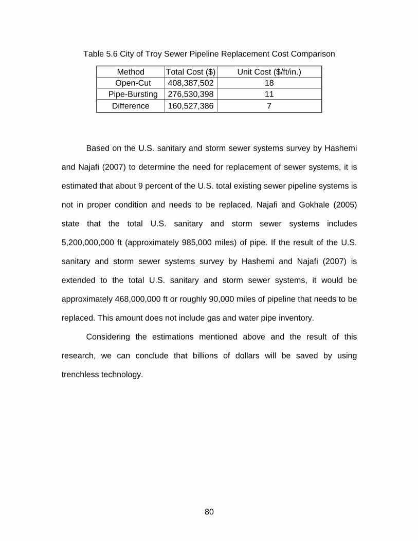
80

Table 5.6 City of Troy Sewer Pipeline Replacement Cost Comparison

Based on the U.S. sanitary and storm sewer systems survey by Hashemi

and Najafi (2007) to determine the need for replacement of sewer systems, it is

estimated that about 9 percent of the U.S. total existing sewer pipeline systems is

not in proper condition and needs to be replaced. Najafi and Gokhale (2005)

state that the total U.S. sanitary and storm sewer systems includes

5,200,000,000 ft (approximately 985,000 miles) of pipe. If the result of the U.S.

sanitary and storm sewer systems survey by Hashemi and Najafi (2007) is

extended to the total U.S. sanitary and storm sewer systems, it would be

approximately 468,000,000 ft or roughly 90,000 miles of pipeline that needs to be

replaced. This amount does not include gas and water pipe inventory.

Considering the estimations mentioned above and the result of this

research, we can conclude that billions of dollars will be saved by using

trenchless technology.

Method Total Cost ($) Unit Cost ($/ft/in.) Open-Cut 408,387,502 18

Pipe-Bursting 276,530,398 11 Difference 160,527,386 7

81

CHAPTER 6

CONCLUSIONS AND RECOMMENDATIONS FOR FUTURE RESEARCH

6.1 Conclusions

This thesis covered a cost analysis for both pipe bursting and open-cut

methods. Computer software was used to develop the regression lines fit on

different combination of variables. A hypothesis test was performed to verify

results of regression analysis which indicated on the average pipe bursting costs

are less than traditional open-cut costs. Based on the results of this research, we

concluded that trenchless pipe-bursting method, in certain conditions, is much

less expensive than the open-cut method for replacing the underground sewer

pipelines.

Based on the results of our research, there is an inverse relationship

between the length of the project and the cost of the project. Open-cut projects

show a sharp cost decrease from $300/ft up to 2,500 ft at $200/ft, then the

decrease in cost becomes gradual as it continues to 10,000 ft to $100/ft. Pipe

bursting costs starts at $200/ft and after a sharp decrease to $100/ft at 1,000 ft

tends to stay the same until 4,000 ft. For cost comparison on diameter size, until

25-inch pipe size both pipe bursting and open-cut methods demonstrate that the

cost steadily increase with diameter of pipe, but the ratio of cost increase versus

the diameter size in open-cut is more than pipe bursting. However; approximately

82

the total cost of pipe bursting, considering diameter, is up to 40% less than open-

cut.

To show how the difference between two methods can potentially save

millions of dollars for municipalities and government agencies, a hypothetical

case study was presented based on the total sewer pipe inventory of City of

Troy, Michigan. The estimated total cost for sewer pipeline replacement in the

City of Troy using the open-cut, the total cost was found to be $403,486,000

while the estimated cost using the pipe bursting technique was estimated as

$242,959,000 with an estimated saving of $160,527,386. With respect to cost of

installation per-inch-per-foot of both methods, pipe bursting shows a cost of $11

per-inch-per-foot while open-cut costs $18 per-inch-per-foot. Consequently, there

is $7 per-inch-per-foot or approximately 40% saving by using pipe bursting.

Looking at the total sanitary sewer inventory in the United States,

approximately 9 percent of the U.S. total existing sewer pipeline systems is not in

proper condition and needs to be replaced. On the other hand, the total U.S.

sanitary and storm sewer systems includes 5,200,000,000 ft (985,000 miles) of

pipe. Therefore, it would be approximately 468,000,000 ft or 90,000 miles of

pipeline that needs to be replaced. This amount does not include gas and water

pipe inventory. The interesting point is that for a relatively small City of Troy with

approximately 400 miles of pipe line, the potential saving from using pipe

bursting was about $160 millions. Therefore, it can be stated that the U.S. can

potentially save billions of dollars by using innovative methods, such as pipe

bursting.

83

In the case study for City of Troy, there was an assumption that the whole

sewer system will be replaced. In reality, the replacement process will be

dependent on the age and condition of specific pipeline sections, along with

many other factors. Therefore, the total budget estimated in this research would

incur over a period of time. Another assumption of the case study is that

replacement and renewal work will be conducted with pipe bursting, while in

reality renewal work may be performed using other trenchless technology

methods (cured-in-place pipe or CIPP, sliplining, close-fit-pipe, point repair, etc.),

or even a new pipeline installed with such methods as microtunneling or

horizontal directional drilling. However, pipe bursting is the only trenchless

method capable of increasing the diameter of an existing pipe, which makes it

more suitable for conditions where existing pipe has inadequate hydraulic

capacity and/or future growth is expected.

6.2 Recommendations for Future Research

One of the major limitations of this study was lack of enough cost data and

project specific conditions for both pipe bursting and open-cut methods. While

we understood this weakness, due to limited time and resources, for comparison

purposes, decided to continue with our cost analysis and develop statistical

models. We recommend future researchers obtain more cost data, and

specifically develop a complete database (such as soil and site conditions,

project conditions, equipment used, problems encountered, etc.) of each project

associated with these cost data. This is specifically important as in reality not two

84

construction project are the same, and we understand that many factors could

change the cost outcome of our analysis. We recommend future researchers to

take upon these important issues.

While for conventional open-cut project increasing the length may in fact

decrease the unit cost ($/ft), for trenchless technology methods, the size factor

may not necessarily be true. For pipe bursting and some trenchless technology

methods larger diameters and longer lengths may make the project more

challenging and may require more sophisticated equipment and experience,

thereby increasing the cost. It is recommended that future researchers consider

these issues in estimating costs.

Notwithstanding these limitations, it appears that there are distinct cost

advantages with trenchless technology. It is important to note that this conclusion

is based only on direct costs of both methods. As in any project, there are

indirect costs that effect the decision making process. Regarding the construction

operation of underground replacement or installation, one of the most important

problems for municipalities is the social costs which have an effect on the total

costs and decision making process of the project. In this research, the

comparison between open-cut and pipe bursting methods was only based on the

direct costs and indirect costs as well as social costs have not been considered.

Therefore, it is expected that pipe bursting technology would be even more cost

effective if these costs had also been considered.

85

APPENDIX A

SIMPLE REGRESSION

86

The Least Squares normal equations are:

0 11 1

n n

i ii i

n x yβ β∧ ∧

= =

+ =∑ ∑

20 1

1 1 1

n n n

i i i ii i i

x X y xβ β∧ ∧

= = =

+ =∑ ∑ ∑

The solution to the Least Squares normal equations is:

0 1ˆ ˆy xβ β= −

that

1 1

11 2

2

2 1

1

ˆ

n n

i ini i

i ii

n

ini

ii

y x

y xn

x

Xn

β

= =

=

=

=

−

= −

∑ ∑∑

∑∑

, 1

1 n

ii

y yn =

= ∑ , 1

1 n

ii

x xn =

= ∑ , 0 1ˆ ˆy xβ β= +

and

2

2

12 2

1 1

( )

n

in ni

xx i ii i

x

S x x xn

=

= =

= − = −∑

∑ ∑

1 1

1 1

( )

n n

i in ni i

xy i i i ii i

y x

S y x y x xn

= =

= =

= − = −∑ ∑

∑ ∑

1xy

xx

S

Sβ =

where

1

1 n

ii

x xn =

= ∑ and 1

1 n

ii

y yn =

= ∑

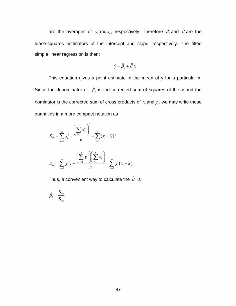
87

are the averages of iy and ix , respectively. Therefore 0β and 1β are the

lease-squares estimators of the intercept and slope, respectively. The fitted

simple linear regression is then:

0 1ˆ ˆy xβ β= +

This equation gives a point estimate of the mean of y for a particular x.

Since the denominator of 1β is the corrected sum of squares of the ix and the

nominator is the corrected sum of cross products of ix and iy , we may write these

quantities in a more compact notation as

2

2

12 2

1 1

1 1

1 1

( )

( )

n

in ni

xx i ii i

n n

i in ni i

xy i i i ii i

x

S x x xn

y x

S y x y x xn

=

= =

= =

= =

= − = −

= − = −

∑∑ ∑

∑ ∑∑ ∑

Thus, a convenient way to calculate the 1β is

1xy

xx

S

Sβ =

88

APPENDIX B

MULTIPLE REGRESSION

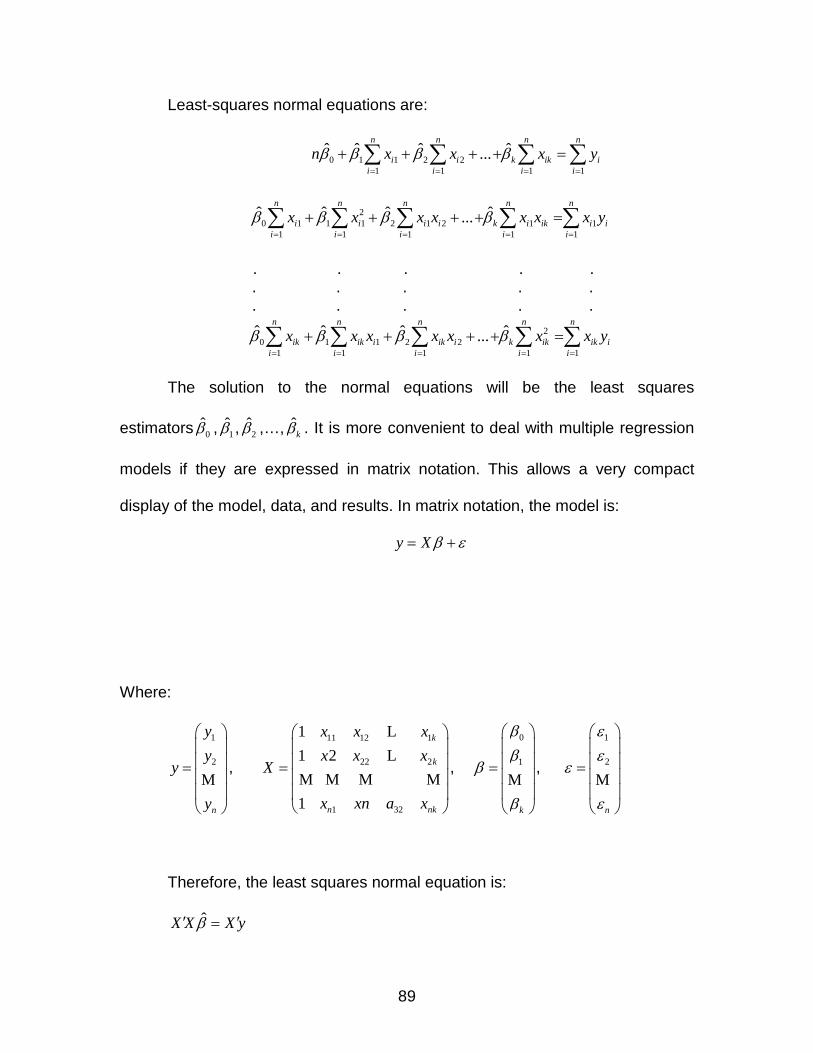
89

Least-squares normal equations are:

0 1 1 2 21 1 1 1

ˆ ˆ ˆ ˆ...n n n n

i i k ik ii i i i

n x x x yβ β β β= = = =

+ + + + =∑ ∑ ∑ ∑

20 1 1 1 2 1 2 1 1

1 1 1 1 1

ˆ ˆ ˆ ˆ...n n n n n

i i i i k i ik i ii i i i i

x x x x x x x yβ β β β= = = = =

+ + + + =∑ ∑ ∑ ∑ ∑

. . . . . . . . . . . . . . .

20 1 1 2 2

1 1 1 1 1

ˆ ˆ ˆ ˆ...n n n n n

ik ik i ik i k ik ik ii i i i i

x x x x x x x yβ β β β= = = = =

+ + + + =∑ ∑ ∑ ∑ ∑

The solution to the normal equations will be the least squares

estimators 0β , 1β , 2β ,…, ˆkβ . It is more convenient to deal with multiple regression

models if they are expressed in matrix notation. This allows a very compact

display of the model, data, and results. In matrix notation, the model is:

y X β ε= +

Where:

1

2

n

y

yy

y

=

M,

11 12 1

22 2

1 32

1

1 2

1

k

k

n nk

x x x

x x xX

x xn a x

=

L

L

M M M M,

0

1

k

β

ββ

β

=

M,

1

2

n

ε

εε

ε

=

M

Therefore, the least squares normal equation is:

ˆX X X yβ′ ′=

90

and in the form of matrix it would be:

01 21 1 1 1

21 1 1 2 1 11

1 1 1 1 1

21 2

1 1 1 1 1

ˆ

ˆ

ˆ

n n n n

i i ik ii i i i

n n n n n

i i i i i ik i ii i i i i

n n n n n

ik ik i ik i ik ik iki i i i i

n x x x y

x x x x x x x y

x x x x x x x y

β

β

β

= = = =

= = = = =

= = = = =

=

∑ ∑ ∑ ∑

∑ ∑ ∑ ∑ ∑

∑ ∑ ∑ ∑ ∑

L

L

M M M M MM

L

Thus, the least squares estimator of β is

( ) 1ˆ X X X yβ −′ ′=

The difference between the observed value iy and the corresponding fitted

value îy is the residual î i ie y y= − . The n residuals may be conveniently written in

matrix notation as

î i ie y y= − or ê y X β= −

91

APPENDIX C

PIPE BURSTING ACTUAL PROJECTS DATA

92

Location Year Name of Project

Length (ft)

Diameter (in.)

Price ($/ft)

Convert to year ratio

2007 Price (S/ft)

Fort Wayne, IN 2000

Sunny Meadows Sanitary Sewer Rehabilitation 2637 12 112 1.37 154.05

Greeley, CO 2001

Sewer Rehabilitation Project 678 6 81 1.33 108.00

Libertyville, IL 2000

Wildwood 15 in. Interceptor Upgrade 88 15 161 1.37 220.83

San Antonio, TX 2000

Briarcroft Emergency Sewer Rehab Project 175 8 112 1.37 153.78


Westlyn Sanitary Sewer Emergency Rehab 1112 8 103 1.33 137.15


Pipe Bursting Construction Contract 3000 10 46 1.29 59.33





San Antonio,TX 2002

Pipe Bursting Construction 1000 21 54 1.29 69.65

San Diego, CA 2002

Sewer Group Job 510 8 100 1.29 128.98

Berkeley, CA 2002

Sanitary Sewer Rehab. and Replacement 1690 6 70 1.29 90.29

Berkeley, CA 2002

Sanitary Sewer Rehab. and Replacement 3620 6 70 1.29 90.29

Boston, MA 2000

Sewer and Waterworks Improvements 910 10 80 1.37 109.84

Boston, MA 2000


Boston, MA 2000


93

Boston, MA 2000


Lancing, MI 2004


Dallas, TX 2000 Lower Five Mile Creek 650 8 138 1.37 189.25



Dallas, TX 2000

Replacement in IH 635,75,35,45E 120 6 66 1.37 91.01

Dallas, TX 2000

Replacement in IH 635,75,35,45E 80 8 85 1.37 116.11

Dallas, TX 2001

Misc. Water and Wastewater Replacement 1550 12 71 1.33 94.74

94

APPENDIX D

PIPE BURSTING AND OPEN-CUT SURVEY ROW DATA

95

Pipe Bursting Project San Francisco, CA Cambridge, MS Dallas, TX Troy, MI

1) Name of the Project Pipe Bursting Project City Hall Sewer &

Drain Replacement Dallas Water Utilities Contract #08-003/004

City of Troy Water Main replacement

2) Year of the Project 2008 2006 2008 2008

3) Location of the Project San Francisco, CA Cambridge, MS Cartwright Street and Drew Street

Troy, MI

4) Type of application (Water, Sanitary Sewer, Storm Sewer, Gas -- other, please specify

Water sanitary sewer & drain Sanitary Sewer Water

5) Total Length of the Project (ft) 3000' 220 ft each 770 2000'

6) Nominal Diameter of the OLD Pipe (in.) 12" 8" SS & 12" SD 6 6"

7) Nominal Diameter of the NEW Pipe (in.) 12" 8" SS & 12" SD 8 8"

8) Average Pipe Depth (from Ground Surface to the Top of the Pipe) ft

10'-14' 5 8'

9) Average Depth of Water Table (from Ground Surface) ft

8' 10 10'

10) Material of the OLD Pipe (Cast Iron, Clay, Concrete, Reinforced Concrete, Asbestos, Ductile Iron, etc., Please Name)

clay & clay Clay Cast Iron

11) Material of the NEW Pipe (HDPE, PVC, Ductile Iron, Clay, Fiber Glass (Hobas), -- other, please specify)

HDPE & HDPE HDPE PVC

12) Soil Conditions (Sandy, Clayey, Gravelly, -- other, please specify)

urban fill w/ silty sand & gravel Clayey Sandy

13) No. of Service Laterals Per Pipe Bursting Drive 3 SD and 1 SS 4

14) Project duration is working days 30 days 10 21

15) Type of Pipe Bursting (Pneumatic, Static, Hydraulic, Pipe Reaming, Pipe Splitting, Tenbusch Method -- other, please specify

Pneumatic Static Static

96

1) Total Cost of Project, including the NEW pipe material cost (Total Bid Price or $/ft)

$65/ft $233,000 or $530/LF $55/ft $50/ft

2) Lateral Installation, if any ($/each) $4,000 SD & $6,250 SS 1320

3) Bypass Pumping, if any ($/day) n/a 0 n/a

4) Point Repairs, if any ($/each, please briefly describe)

n/a 1475 n/a

5) Pit Excavation & Shoring ($/each, please specify the size of the pit)

$118,175 incl common

manhole separation 0 500

6) Pit Reinstatement (backfill, compaction, pavement, etc.) ($/each or per sq ft)

$31,000 surface restoration

3.7 500

7) SOCIAL Costs such as traffic disruptions, inconvenience to public (please provide if available)

n/a n/a

8) Other Costs (please briefly explain)

Actual P/B cost was $66,000 for both SS & SD-Existing conditions

were a 8" SS under a 12" SD with 6" separation.

Pit cost includes common manhole separation. Exit

location was MH.

0

Open-Cut Project Bellevue, WA Cambridge, MS Dallas, TX Greeley, CO

1) Name of the Project

Bellevue Pump Station Force Main

City Hall Sewer & Drain Replacement

Dallas Water Utilities Contract

#08-003/004

2008 Sanitary Sewer

Rehabilitation Projects


3) Location of the Project Bellevue, WA Cambridge, MA Dallas, TX Madison Avenue

residential, Greeley, CO

4) Type of application (Water, Sanitary Sewer, Storm Sewer, Gas, -- other, please specify)

SS Sanitary sewer & storm drain

Water and Sanitary Sewer Sanitary Sewer

5) Total Length of the Project (ft)

500 220 LF each 915 1729

6) Nominal Diameter of the OLD Pipe (in.) 8" SS under 12" SD 6 4

7) Nominal Diameter of the NEW Pipe (in.) 24 8" SS & 12" SD 8 8

8) Width Size of the Trench (respectively; at the Top of Trench-at the Bottom of the Trench-at the Depth of the Trench) ft

8 n/a 4.5-2-2.5 8' top 8' bottom 9.5' deep

9) Average Pipe Depth (from Ground Surface to Top of the Pipe) ft

5 10'-14' 4 9.5


5'-6' 8' 10 n/a

11) Material of the OLD Pipe (Cast Iron, Clay, Concrete, Reinforced Concrete, Asbestos, Ductile Iron, -- other, please specify)

Clay Cast Iron/Clay Clay

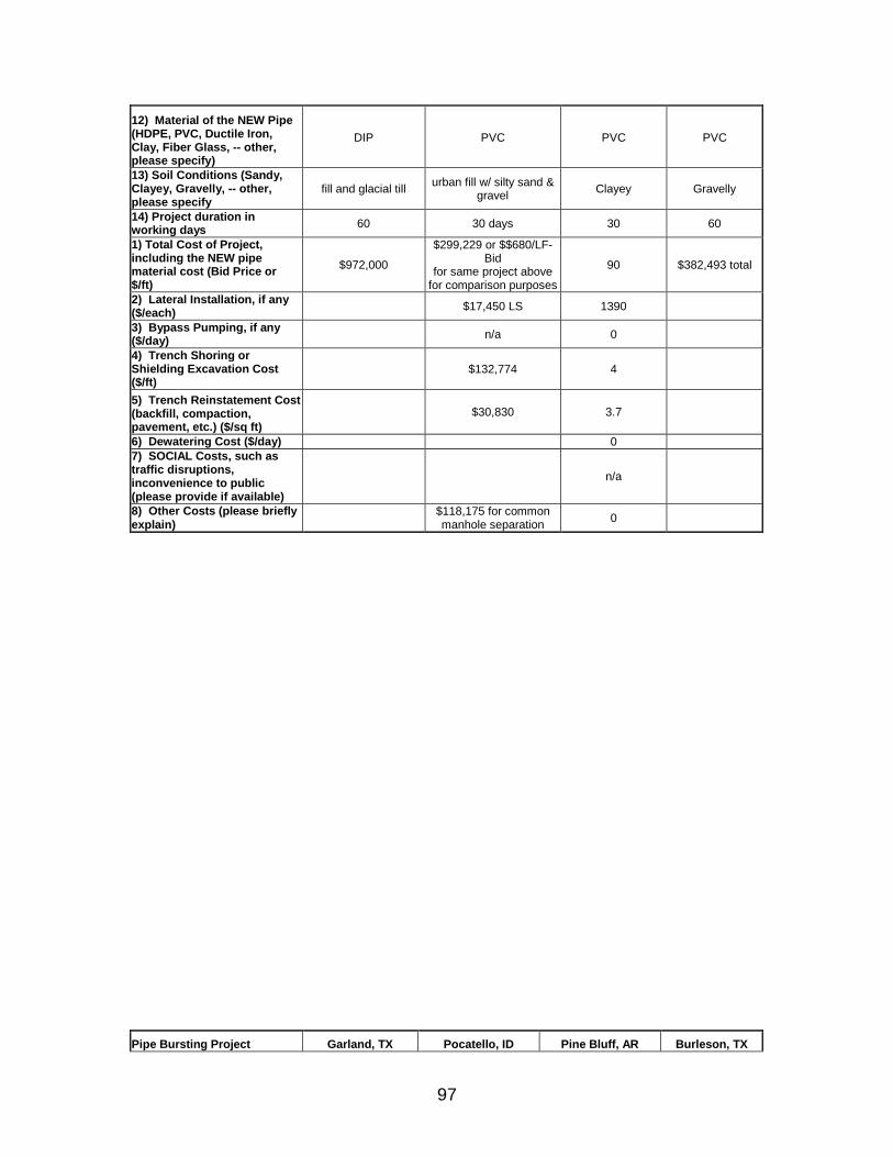
97

12) Material of the NEW Pipe (HDPE, PVC, Ductile Iron, Clay, Fiber Glass, -- other, please specify)

DIP PVC PVC PVC

13) Soil Conditions (Sandy, Clayey, Gravelly, -- other, please specify

fill and glacial till urban fill w/ silty sand & gravel Clayey Gravelly

14) Project duration in working days 60 30 days 30 60

1) Total Cost of Project, including the NEW pipe material cost (Bid Price or $/ft)

$972,000

$299,229 or $$680/LF-Bid

for same project above for comparison purposes

90 $382,493 total

2) Lateral Installation, if any ($/each) $17,450 LS 1390

3) Bypass Pumping, if any ($/day) n/a 0

4) Trench Shoring or Shielding Excavation Cost ($/ft)

$132,774 4

5) Trench Reinstatement Cost (backfill, compaction, pavement, etc.) ($/sq ft)

$30,830 3.7

6) Dewatering Cost ($/day) 0 7) SOCIAL Costs, such as traffic disruptions, inconvenience to public (please provide if available)

n/a


$118,175 for common manhole separation 0

Pipe Bursting Project Garland, TX Pocatello, ID Pine Bluff, AR Burleson, TX

98

1) Name of the Project Leon Pipe Burst

Downtown Sanitary Sewer Rehab Phases

II and III

2006 Pipe Bursting Project

Elk Ridge Relief Sewer


3) Location of the Project Leon/Wall, Garland,

TX Pocatello, ID Pine Bluff, AR Burleson, TX

4) Type of application (Water, Sanitary Sewer, Storm Sewer, Gas -- other, please specify

Sanitary Sewer Sanitary Sewer Sanitary Sewer Water

5) Total Length of the Project (ft) 1590 700 3596 4500

6) Nominal Diameter of the OLD Pipe (in.) 8 8 6 12

7) Nominal Diameter of the NEW Pipe (in.) 10 8 8 12


14 14 6


20 35 Unknown

10) Material of the OLD Pipe (Cast Iron, Clay, Concrete, Reinforced Concrete, Asbestos, Ductile Iron, etc., Please Name)

VCT Clay Clay Clay

11) Material of the NEW Pipe (HDPE, PVC, Ductile Iron, Clay, Fiber Glass (Hobas), -- other, please specify)

HDPE HDPE HDPE HDPE


Clayey Gravely Sandy

13) No. of Service Laterals Per Pipe Bursting Drive 1 6 8

14) Project duration is working days 10 30 60

15) Type of Pipe Bursting (Pneumatic, Static, Hydraulic, Pipe Reaming, Pipe Splitting, Tenbusch Method -- other, please specify

Pneumatic Pneumatic Pneumatic


$95,410 total $105 $208,126 $100

2) Lateral Installation, if any ($/each) 177 $300 each

3) Bypass Pumping, if any ($/day) 250 None

4) Point Repairs, if any ($/each, please briefly describe)

$5,000, Point repairs were done on Main

Line pipe that was not included in the pipe

bursting lines.

None


included in pipe cost $10,000

6) Pit Reinstatement (backfill, compaction, pavement, etc.) ($/each or per sq ft)

$6.00 $10,000

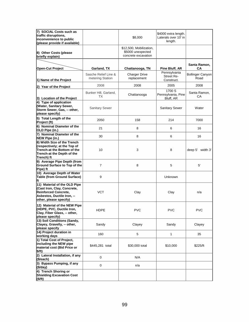
99

7) SOCIAL Costs such as traffic disruptions, inconvenience to public (please provide if available)

$8,000 $4000 extra length. Laterals over 10' in

length.


$12,500, Mobilization,

$5000 unexpected concrete excavation

Open-Cut Project Garland, TX Chattanooga, TN Pine Bluff, AR

Santa Ramon, CA


Sasche Relief Line & metering Station

Charger Drive replacement

Pennsylvania Street Re-Construct.

Bollinger Canyon Road


3) Location of the Project

Bunker Hill, Garland, TX

Chattanooga 1700 S

Pennsylvania, Pine Bluff, AR

Santa Ramon, CA


Sanitary Sewer Sanitary Sewer Water


2050 158 214 7000

6) Nominal Diameter of the OLD Pipe (in.) 21 8 6 16

7) Nominal Diameter of the NEW Pipe (in.) 30 8 6 16


10 3 8 deep 5' width 3'


7 8 5 5'


9 Unknown


VCT Clay Clay n/a


HDPE PVC PVC PVC


Sandy Clayey Sandy Clayey

14) Project duration in working days 160 5 1 35


$445,281 total $30,000 total $10,000 $225/ft

2) Lateral Installation, if any ($/each) 0 N/A

3) Bypass Pumping, if any ($/day) 0 n/a


100


8520

6) Dewatering Cost ($/day) 0 7) SOCIAL Costs, such as traffic disruptions, inconvenience to public (please provide if available)

None


$619,015-abandon siphon & construct

aerial creek crossing & add Gabion retaining

walls

Open-Cut Project San Francisco, CA Mesquite, NV


San Francisco Airport Project Mesquite, NV

2) Year of the Project 2008 2008

3) Location of the Project San Francisco Airport Mesquite


Water


10000 4000

6) Nominal Diameter of the OLD Pipe (in.) 12 16

7) Nominal Diameter of the NEW Pipe (in.)

12 16






PVC


14) Project duration in working days


$120/ft $110/ft

101

APPENDIX E

PIPE BURSTING AND OPEN-CUT SURVEY QUESTIONAIRE

102

Construction Cost Comparison of Open-Cut and Pipe Bursting for Municipal Water, Sewer and Gas

Applications

Project OverviewProject OverviewProject OverviewProject Overview

The Center for Underground Infrastructure Research and Education (CUIRE) at The University of Texas at Arlington on a project entitled "Construction Cost Comparison of Open-Cut and Pipe Bursting for Municipal Water, Sewer and Gas Applications," The main objective of this project is to provide a comprehensive study and decision making procedures for cost comparison of trenchless technology methods for replacement of municipal water, wastewater and gas infrastructures.

This national survey will provide valuable information regarding the asset management of underground infrastructure and use of trenchless technologies. There are few questions in this survey and we estimate that it will take around 20-25 minutes to complete. There are no risks or individual benefits by associated with completing this survey.

We will acknowledge your help in completing this questionnaire in our final report, but we will not refer to your individual responses, therefore, your input will be anonymous. Once again, we greatly appreciate your help in advance and we will send you a copy of the final report scheduled for late fall 2008.

If you have any question or concern, please feel free to contact CUIRE director, Dr. Mohammad Najafi directly at 817-272-0507 and [email protected] or graduate student in charge of the survey, Behnam Hashemi at 817-272-9164 and [email protected]

Contact Person’s Name Position

Phone E-mail

103

Part A:Part A:Part A:Part A: Pipe Bursting Actual Project ExamplePipe Bursting Actual Project ExamplePipe Bursting Actual Project ExamplePipe Bursting Actual Project Example


2) Year of the Project

3) Location of the Project 4) Type of application (Water, Sanitary Sewer, Storm Sewer, Gas -- other, please specify)


6) Nominal Diameter of the OLD Pipe (in.)

7) Nominal Diameter of the NEW Pipe (in.)


9) Average Depth of Water Table (from Ground Surface) ft 10) Material of the OLD Pipe (Cast Iron, Clay, Concrete, Reinforced Concrete, Asbestos, Ductile

Iron, etc., Please Name) 11) Material of the NEW Pipe (HDPE, PVC, Ductile Iron, Clay, Fiber Glass (Hobas), -- other,

please specify)


13) No. of Service Laterals Per Pipe Bursting Drive

14) Project duration is working days 15) Type of Pipe Bursting (Pneumatic*, Static*, Hydraulic*, Pipe Reaming*, Pipe Splitting*,

Tenbusch Method* -- other, please specify)) • For description of Pipe Bursting terms please refer to the bottom of the page! Pipe Bursting Cost Data: Pipe Bursting Cost Data: Pipe Bursting Cost Data: Pipe Bursting Cost Data:


Name of Organization

Type of Organization (owner, consulting/design engineer, contractor, manufacturer (other, please specify)

City State choose one

Zip

104

It would be more helpful if you provide detailed price as follows:

2) Lateral Installation, if any ($/each)

3) Bypass Pumping, if any ($/day) 4) Point Repairs, if any ($/each, please briefly describe)


6) Pit Reinstatement (backfill, compaction, pavement, etc.) ($/each or per sq ft) 7) SOCIAL Costs such as traffic disruptions, inconvenience to public (please provide if available)

8) Other Costs (please briefly explain) Part B:Part B:Part B:Part B: OpeOpeOpeOpennnn----Cut Project Actual Project ExampleCut Project Actual Project ExampleCut Project Actual Project ExampleCut Project Actual Project Example


2) Year of the Project

3) Location of the Project 4) Type of application (Water, Sanitary Sewer, Storm Sewer, Gas, -- other, please specify)


6) Nominal Diameter of the OLD Pipe (in.)

7) Nominal Diameter of the NEW Pipe (in.) 8) Width Size of the Trench (respectively; at the Top of Trench-at the Bottom of the Trench-at the

Depth of the Trench) ft


10) Average Depth of Water Table (from Ground Surface) ft 11) Material of the OLD Pipe (Cast Iron, Clay, Concrete, Reinforced Concrete, Asbestos, Ductile

Iron, -- other, please specify) 12) Material of the NEW Pipe (HDPE, PVC, Ductile Iron, Clay, Fiber Glass, -- other, please

specify)


14) Project duration in working days OpenOpenOpenOpen----Cut Cost Data: Cut Cost Data: Cut Cost Data: Cut Cost Data:


105

It would be more helpful if you provide any price details as follows:

2) Lateral Installation, if any ($/each)

3) Bypass Pumping, if any ($/day)



6) Dewatering Cost ($/day) 7) SOCIAL Costs, such as traffic disruptions, inconvenience to public (please provide if available)


106

APPENDIX F

ABBREVIATIONS

107

ABS Acrylonitrile Butadiene Styrene ACP Asbestos Cement Pipe ASCE American Society of Civil Engineers CIPP Cured In Place Pipe CLG Controlled Line and Grade CP Concrete Pipe DIP Ductile Iron Pipe DR Diameter thickness Ratio HEB Horizontal Earth Boring HDD Horizontal Directional Drilling HDPE High Density Polyethylene ID Inside Diameter L2 Length Square LD Logarithm Diameter LL Logarithm Length NASTT North American Society of Trenchless Technology OD Outside Diameter OSHA Occupational Safety and Health Administration PCCP Prestressed Concrete Cylinder Pipe PE Polyethylene PJ Pipe Jacking PVC Poly Vinyl Chloride RCCP Reinforced Concrete Cylinder Pipe RCP Reinforced Concrete Pipe SAS Statistical Analysis System TCM Trenchless Construction Methods TLP Tunnel Liner Plates TRM Trenchless Renewal Methods TTC Trenchless Technology Center UT Utility Tunneling UCP Unreinforced Concrete Pipe VCP Vitrified clay pipe

108

APPENDIX G

SAS CODES FOR PIPE BURSTING MODEL

109

data BPPPP; input cost length diameter; l2=length*length; LD=log (diameter); LL=log (length); cards ; 154.05 2637 12 108 678 6 220.83 88 15 153.78 175 8 137.15 1112 8 59.33 3000 10 90.62 1000 12 164.49 1000 18 69.65 1000 21 128.98 510 8 90.29 1690 6 90.29 3620 6 109.84 910 10 137.3 910 15 178.49 790 18 205.96 944 12 194.48 310 18 189.25 650 8 124.95 500 18 144.17 600 21 91 120 6 116.11 80 8 94.74 1550 12 100 4500 12 54 770 6 59 1590 8 102 700 8 60 3596 6 59 2000 6 63 3000 12 ; proc means data =BPPPP; var length; output out =stats mean=mleng; data BPPPP1; set BPPPP; if (_n_ eq 1) then set stats; leng=length-mleng; leng2=leng*leng; proc print; proc corr data =BPPPP1 noprob ; var cost leng diameter leng2; proc print; proc iml; use BPPPP1; read all var{cost} into y; read all var{leng diameter leng2} into X; n=nrow(X); X=J(n, 1) || X;

110

print X; p=ncol(X); xpx=X`*X; print xpx; xpxi=inv(xpx); print xpxi; xpy=X`*y; print xpy; b=xpxi*xpy; print b; store ; quit; proc reg data =BPPPP1; model cost = leng diameter leng2 / ss1 vif i ; output out =costout predicted =yhat residual =e student =tres h=hii cookd =cookdi dffits =dffitsi; proc reg data =BPPPP1; model cost = leng diameter / ss1 vif i cli ; output out =costout predicted =yhat residual =e student =tres h=hii cookd =cookdi dffits =dffitsi; run; proc reg data =BPPPP1; model cost = LD LL / ss1 vif i cli ; output out =costout predicted =yhat residual =e student =tres h=hii cookd =cookdi dffits =dffitsi; run; data cost2; set costout; x1x2= length*diameter; run; proc plot data =costout; plot e*yhat; run; proc plot data =costout; plot cost*leng= 'a' yhat*leng= 'p' / overlay ; run;

111

APPENDIX H

SAS DATA MATRIX FOR PIPE BURSTING

112

The SAS System 13:30 Tuesday, October 28, 2008

Obs cost length diameter l2 LD _TYPE_ _FREQ_ mleng leng leng2 1 154.05 2637 12 6953769 2.48491 0 28 1386.07 1250.93 1564822.29 2 108.00 678 6 459684 1.79176 0 28 1386.07 -708.07 501365.15 3 220.83 88 15 7744 2.70805 0 28 1386.07 -1298.07 1684989.43 4 153.78 175 8 30625 2.07944 0 28 1386.07 -1211.07 1466694.01 5 137.15 1112 8 1236544 2.07944 0 28 1386.07 -274.07 75115.15 6 59.33 3000 10 9000000 2.30259 0 28 1386.07 1613.93 2604765.43 7 90.62 1000 12 1000000 2.48491 0 28 1386.07 -386.07 149051.15 8 164.49 1000 18 1000000 2.89037 0 28 1386.07 -386.07 149051.15 9 69.65 1000 21 1000000 3.04452 0 28 1386.07 -386.07 149051.15 10 128.98 510 8 260100 2.07944 0 28 1386.07 -876.07 767501.15 11 90.29 1690 6 2856100 1.79176 0 28 1386.07 303.93 92372.58 12 90.29 3620 6 13104400 1.79176 0 28 1386.07 2233.93 4990436.86 13 137.30 910 15 828100 2.70805 0 28 1386.07 -476.07 226644.01 14 178.49 790 18 624100 2.89037 0 28 1386.07 -596.07 355301.15 15 205.96 944 12 891136 2.48491 0 28 1386.07 -442.07 195427.15 16 189.25 650 8 422500 2.07944 0 28 1386.07 -736.07 541801.15 17 124.95 500 18 250000 2.89037 0 28 1386.07 -886.07 785122.58 18 144.17 600 21 360000 3.04452 0 28 1386.07 -786.07 617908.29 19 91.00 120 6 14400 1.79176 0 28 1386.07 -1266.07 1602936.86 20 116.11 80 8 6400 2.07944 0 28 1386.07 -1306.07 1705822.58 21 94.74 1550 12 2402500 2.48491 0 28 1386.07 163.93 26872.58 22 100.00 4500 12 20250000 2.48491 0 28 1386.07 3113.93 9696551.15 23 54.00 770 6 592900 1.79176 0 28 1386.07 -616.07 379544.01 24 59.00 1590 8 2528100 2.07944 0 28 1386.07 203.93 41586.86 25 102.00 700 8 490000 2.07944 0 28 1386.07 -686.07 470694.01 26 60.00 3596 6 12931216 1.79176 0 28 1386.07 2209.93 4883784.29 27 59.00 2000 6 4000000 1.79176 0 28 1386.07 613.93 376908.29 28 63.00 3000 12 9000000 2.48491 0 28 1386.07 1613.93 2604765.4

113

APPENDIX I

SAS MATRIX METHOD OUTPUT FOR PIPE BURSTING MODEL

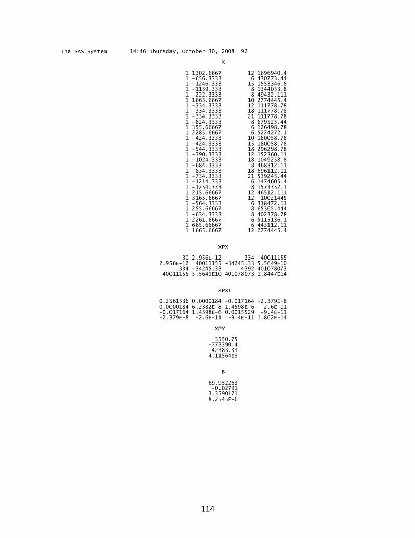
114

The SAS System 14:46 Thursday, October 30, 2008 92 X 1 1302.6667 12 1696940.4 1 -656.3333 6 430773.44 1 -1246.333 15 1553346.8 1 -1159.333 8 1344053.8 1 -222.3333 8 49432.111 1 1665.6667 10 2774445.4 1 -334.3333 12 111778.78 1 -334.3333 18 111778.78 1 -334.3333 21 111778.78 1 -824.3333 8 679525.44 1 355.66667 6 126498.78 1 2285.6667 6 5224272.1 1 -424.3333 10 180058.78 1 -424.3333 15 180058.78 1 -544.3333 18 296298.78 1 -390.3333 12 152360.11 1 -1024.333 18 1049258.8 1 -684.3333 8 468312.11 1 -834.3333 18 696112.11 1 -734.3333 21 539245.44 1 -1214.333 6 1474605.4 1 -1254.333 8 1573352.1 1 215.66667 12 46512.111 1 3165.6667 12 10021445 1 -564.3333 6 318472.11 1 255.66667 8 65365.444 1 -634.3333 8 402378.78 1 2261.6667 6 5115136.1 1 665.66667 6 443112.11 1 1665.6667 12 2774445.4 XPX 30 2.956E-12 334 40011155 2.956E-12 40011155 -34245.33 5.5649E10 334 -34245.33 4392 401078073 40011155 5.5649E10 401078073 1.8447E14 XPXI 0.2561536 0.0000184 -0.017164 -2.379E-8 0.0000184 6.2382E-8 1.4598E-6 -2.6E-11 -0.017164 1.4598E-6 0.0015529 -9.4E-11 -2.379E-8 -2.6E-11 -9.4E-11 1.862E-14 XPY 3550.75 -772390.4 42383.33 4.11564E9 B 69.952263 -0.02791 3.3590171 8.2545E-6

115

APPENDIX J

SAS CODES FOR OPEN-CUT MODEL

116

data BPPPP; input cost length diameter; l2=length*length; LD=log (diameter); LL=log (length); cards ; 434 220 8 650 220 12 87 915 6 214 1729 6 210 2050 24 184 158 8 50 214 6 218 7000 16 116 10000 12 ; proc means data =BPPPP; var length; output out =stats mean=mleng; data BPPPP1; set BPPPP; if (_n_ eq 1) then set stats; leng=length-mleng; leng2=leng*leng; proc print; proc corr data =BPPPP1 noprob ; var cost leng diameter leng2; proc print; proc iml; use BPPPP1; read all var{cost} into y; read all var{leng diameter leng2} into X; n=nrow(X); X=J(n, 1) || X; print X; p=ncol(X); xpx=X`*X; print xpx; xpxi=inv(xpx); print xpxi; xpy=X`*y; print xpy; b=xpxi*xpy; print b; store ; quit; proc reg data =BPPPP1; model cost = leng diameter leng2 / ss1 vif i ; output out =costout predicted =yhat residual =e student =tres h=hii cookd =cookdi dffits =dffitsi;

117

proc reg data =BPPPP1; model cost = leng diameter / ss1 vif i cli ; output out =costout predicted =yhat residual =e student =tres h=hii cookd =cookdi dffits =dffitsi; run; proc reg data =BPPPP1; model cost = LD LL / ss1 vif i cli ; output out =costout predicted =yhat residual =e student =tres h=hii cookd =cookdi dffits =dffitsi; run; data cost2; set costout; x1x2= length*diameter; run; proc plot data =costout; plot e*yhat; run; proc plot data =costout; plot cost*leng= 'a' yhat*leng= 'p' / overlay ; run;

118

APPENDIX K

SAS DATA MATRIX FOR OPEN-CUT

119

Obs cost length diameter l2 LD LL _TYPE_ _FREQ_ mleng leng leng2 1 434 220 8 48400 2.07944 5.39363 0 9 2500.67 -2280.67 5201440.44 2 650 220 12 48400 2.48491 5.39363 0 9 2500.67 -2280.67 5201440.44 3 87 915 6 837225 1.79176 6.81892 0 9 2500.67 -1585.67 2514338.78 4 214 1729 6 2989441 1.79176 7.45530 0 9 2500.67 -771.67 595469.44 5 210 2050 24 4202500 3.17805 7.62560 0 9 2500.67 -450.67 203100.44 6 184 158 8 24964 2.07944 5.06260 0 9 2500.67 -2342.67 5488087.11 7 50 214 6 45796 1.79176 5.36598 0 9 2500.67 -2286.67 5228844.44 8 218 7000 16 49000000 2.77259 8.85367 0 9 2500.67 4499.33 20244000.44 9 116 10000 12 100000000 2.48491 9.21034 0 9 2500.67 7499.33 56240000.44

120

APPENDIX L

SAS MATRIX METHOD OUTPUT FOR OPEN-CUT MODEL

121

The SAS System 14:46 Thursday, October 30, 2008 54 X 1 -2280.667 8 5201440.4 1 -2280.667 12 5201440.4 1 -1585.667 6 2514338.8 1 -771.6667 6 595469.44 1 -450.6667 24 203100.44 1 -2342.667 8 5488087.1 1 -2286.667 6 5228844.4 1 4499.3333 16 20244000 1 7499.3333 12 56240000 XPX 9 2.274E-12 98 100916722 2.274E-12 100916722 58946.667 4.5977E11 98 58946.667 1356 1.20162E9 100916722 4.5977E11 1.20162E9 3.691E15 XPXI 1.5166459 0.0002783 -0.076233 -5.132E-8 0.0002783 7.956E-8 -0.000011 -1.38E-11 -0.076233 -0.000011 0.0051201 1.8265E-9 -5.132E-8 -1.38E-11 1.8265E-9 2.803E-15 XPY 2163 -1564579 24770 1.8235E10 B 20.902765 -0.054971 12.93935 7.004E-6

122

APPENDIX M

PIPE BURSTING REGRESSION CALCULATION

123

Number Diameter (in.)

Length (ft)

Adjusted Diameter

Diameter Ratio

Adjusted Length

Length Ratio

Diameter Logarithm

Length Logarithm

9.4 E-06 X Length Square

Regression Total Price

1 3 1,900 6 0.5 1,900 1.00 1.7917595 7.5496092 33.934000 30 56,063 2 6 7,810 6 1.00 5,000 1.12 1.7917595 8.5171932 235.000000 80 626,498 3 8 1,194,414 8 1.00 5,000 170.63 2.0794415 8.5171932 235.000000 109 130,035,144 4 10 219,310 10 1.00 5,000 31.33 2.3025851 8.5171932 235.000000 125 27,425,955 5 12 431,924 12 1.00 5,000 61.70 2.4849066 8.5171932 235.000000 133 57,600,093 6 15 81,958 15 1.00 5,000 11.71 2.7080502 8.5171932 235.000000 136 11,153,333 7 17 319 17 1.00 319 1.00 2.8332133 5.7651911 0.956553 166 52,959 8 20 71 20 1.00 71 1.00 2.9957323 4.2626799 0.047385 165 11,724 9 21 20,857 21 1.00 5,000 2.98 3.0445224 8.5171932 235.000000 120 2,509,781

10 24 16,010 24 1.00 5,000 2.29 3.1780538 8.5171932 235.000000 106 1,693,103 11 27 13,737 24 1.125 5,000 1.96 3.1780538 8.5171932 235.000000 119 1,634,318 12 30 11,140 24 1.25 5,000 1.59 3.1780538 8.5171932 235.000000 132 1,472,609 13 36 22,256 24 1.5 5,000 3.18 3.1780538 8.5171932 235.000000 159 3,530,454 14 42 2,767 24 1.75 2,767 1.00 3.1780538 7.925519 71.969117 127 351,931 15 48 11,563 24 2 5,000 1.65 3.1780538 8.5171932 235.000000 212 2,445,641 16 60 10,859 24 2.5 5,000 1.55 3.1780538 8.5171932 235.000000 264 1,640,529 17 66 1,397 24 2.75 1,397 1.00 3.1780538 7.2420824 18.345125 268 214,207 18 72 1,900 24 3 1,900 1.00 3.1780538 7.5496092 33.934000 254 275,390 19 78 1,178 24 3.25 1,178 1.00 3.1780538 7.0715734 13.044230 340 228,825

Total 2,051,370 242,958,558

124

APPENDIX N

OPEN-CUT REGRESSION CALCULATION

125

Diameter (inch)

Length (foot)

Adjusted Diameter

Diameter Ratio

Adjusted Length

Length Ratio

Diameter Logarithm

Length Logarithm

1.0 E-05X Length Square Regression Total ($)

3 1,900 6 0.5 1900 1 1.791759 7.549609 180.5 70 133,326 6 7,810 6 1 7810 1 1.791759 8.96316 3049.805 140 1,096,080 8 1,194,414 8 1 10000 119.44 2.079442 9.21034 5000 166 198,134,675

10 219,310 10 1 10000 21.931 2.302585 9.21034 5000 189 41,417,906 12 431,924 12 1 10000 43.192 2.484907 9.21034 5000 210 90,689,536 15 81,958 15 1 10000 8.1958 2.70805 9.21034 5000 239 19,591,392 17 319 17 1 319 1 2.833213 5.765191 5.08805 257 82,008 20 71 20 1 71 1 2.995732 4.26268 0.25205 283 20,061 21 20,857 21 1 10000 2.0857 3.044522 9.21034 5000 291 6,062,551 24 16,010 24 1 10000 1.601 3.178054 9.21034 5000 314 5,029,210 27 13,737 24 1.125 10000 1.3737 3.178054 9.21034 5000 353 4,854,594 30 11,140 24 1.25 10000 1.114 3.178054 9.21034 5000 393 4,374,251 36 22,256 24 1.5 10000 2.2256 3.178054 9.21034 5000 471 10,486,893 42 2,767 24 1.75 2767 1 3.178054 7.925519 382.81445 550 1,521,093 48 11,563 24 2 10000 1.1563 3.178054 9.21034 5000 628 7,264,555 60 10,859 24 2.5 10000 1.0859 3.178054 9.21034 5000 785 8,527,826 66 1,397 24 2.75 1397 1 3.178054 7.242082 97.58045 864 1,206,806 72 1,900 24 3 1900 1 3.178054 7.549609 180.5 942 1,790,537 78 1,178 24 3.25 1178 1 3.178054 7.071573 69.3842 1,021 1,202,644

Total 2,051,370 403,485,944

126

APPENDIX O

SURVEY RESPONDENTS

127

Name Organization City State James Chae Jacobs Engineering Group Bellevue Washington

John Struzziery S E A Consultants Inc. Cambridge Mississippi Marty Paris Kimley-Horn and Associates, Inc. Dallas Texas Tony Braun City of Greeley Greeley Colorado

Brent Erickson City of Garland Garland Texas Mike Patrick City of Chattanooga Chattanooga Tennessee

Jesse Schuerman City of Pocatello Pocatello Idaho David Poe Pine Bluff Wastewater Utility Pine Bluff Arkansas

Mike Garrett Underground Solutions Poway California

128

REFERENCES Adedapo, A. A. (2007). Pavement deterioration and PE pipe behavior resulting from open-cut and HDD pipeline installation techniques. Waterloo, Ontario, Canada. Retrieved from ASCE database, September 30, 2008. Atalah, A. (2004). Ground movement in hard rock conditions related to Pipe bursting., ASCE Pipelines 2004., Retrieved from ASCE database,

October 10, 2008. City of Troy Website. (2007). http://en.wikipedia.org/wiki/Troy,_Michigan. Retrieved April 15, 2008. Cody, R. (2007). Learning SAS by Examples: A programmer’s guide. Cary SAS Institute, North Carolina. Gangavarapu, B. S. (2003). Analysis and comparison of traffic disruption using open-cut and trenchless methods of pipe installation. ProQuest Information and Learning Company. Ann Arbor, MI. Harrell, F. E. (2001). Statistical tools for nonlinear regression. Spring-Verlag New York, Inc., New York. Hashemi, B., and Najafi, M. (2007). U.S. sanitary and storm sewer systems survey. Trenchless Technology Magazine. Vol. 15, page 34-38. October, 2007. Howard, A. (1996). Pipeline Installation. Relativity Publishing., Lake Wood, Colorado. Huet, S., Bouvier, A., Poursat, M. A., and Jolivet, E. (2003). Regression Modeling Strategies: with application to linear models, logistic regression, and survival analysis. Spring-Verlag New York, Inc., New York.

Jung, Y., Sinha, S. (2007). Evaluation of Trenchless Technology Methods for Municipal Infrastructure System. Journal of Infrastructure Systems, Vol. 13, No. 2, pp. 144-156.

Lee H., Najafi, M., & Matthys, J. (2007). Cost comparison of pipeline asset replacement: open-cut and pipe-bursting. Proceedings of ASCE International Pipeline 2007 Conference, Boston, Massachusetts.

129

McKim, R. A. (1997). Selection method for trenchless technologies. Journal of Infrastructure Systems, Vol. 3, No. 3, pp. 119-125.

Montgomery, D. C., Peck, E. A., and Vining, G. G. (2006). Introduction to linear regression analysis. John Wiley & Sons, Inc. Hoboken, New Jersey. Muller, K. E., Fetterman, B. A. (2003). Regression and ANOVA: an integrated approach using SAS software. SAS Institute Inc and Wisely. Cary, NC. Najafi, M., & Gokhale, S. (2005). Trenchless technology: pipeline and utility

design, construction and renewal. McGraw-Hill, New York. Najafi, M., & American Society of Civil Engineers (ASCE). (2007). Pipe Bursting

Projects., American Society of Civil Engineers., Reston, VA. Najafi, M. and Kim, K. O. (2004). Life-Cycle-Cost Comparison of Trenchless and

Conventional Open-Cut Pipeline Construction Projects. Retrieved from ASCE database September 30, 2008.

Oxford Plastics Inc. Web site. (2007).

http://www.oxfordplasticsinc.com/pipebursting.htm, Retrieved May, 29 2008.

R. S. Means Database. (2007). Site work & landscape cost data. Construction

Publishers & Consultants, Kingston, MA. ASCE R. S. Means. (2007). Building Construction Cost Data. Reed Construction Data, Inc. Kingston, MA. Simicevic, J., & Sterling, R. (2001). Guideline for pipe bursting. U.S. Army Corps

of Engineers Engineering Research and Development Center (ERDC). Vicksburg, MS.

Spector, P. E. (2001). SAS programming for researchers and social scientists. Sage Publications, Inc. Thousands Oaks, CA. Trenchless Technology Center (TTC) website. (2008).

http://www.coes.latech.edu/ttc. Retrieved July 20, 2008. TT Technologies Co. Web site. (2008).

http://tttechnologies.com/jstories/gcrack/index.html, Retrieved July, 20 2008.

130

Woodroffe, N. J. A., & Ariaratnam, S. T. (2008). Cost and Risk Evaluation for Horizontal Directional Drilling versus Open Cut in an Urban Environment, Practice Periodical on Structural Design and Construction © ASCE / MAY 2008 / pp. 85-92. Retrieved from ASCE database September 30, 2008. Zhao, J. Q., Rajani, B. (2002). Construction and rehabilitation costs for buried

pipe with a focus on trenchless technologies. Institute for Research in Construction National Research Council Canada, Ottawa, Canada.

131

BIOGRAPHICAL INFORMATION

Behnam Hashemi received his B.S. degree in Industrial Engineering from

Azad University of Esfahan, Iran in 2002. In 2006, he graduated from the same

university with a M.S. in Industrial Engineering. He came to the U.S.A for

continuing his studies in Construction Engineering and Management area of Civil

Engineering.

Although he had experiences in project control and manufacturing, he

started to work on Trenchless Technology with Dr. Mohammad Najafi at the

Center of Underground Infrastructure Research and Education (CUIRE), and

completed several research projects. He has published and presented several

papers in the ASCE international Pipeline Conferences and Underground

Construction Technology (UCT) seminars related to U.S. sanitary and storm

sewer systems survey and cost comparison of trenchless technology with

traditional methods.

His plan is to continue his education towards a PhD along with working in

the industry to learn and contribute the theory and practice of construction

engineering and Trenchless Technology.

Documents

CONSTRUCTION COST OF UNDERGROUND INFRASTRUCTURE by …