Construction and Control of an Inverted Pendulumcontrol.lth.se/documents/2000/5679.pdf · Construction and Control of an Inverted Pendulum Carina Hansen ... This solution makes it

ISSN 0280-5316ISRN LUTFD2/TFRT--5679--SE

Construction and Controlof an Inverted Pendulum

Carina HansenCecilia Svensson

Department of Automatic ControlLund Institute of Technology

July 2000

Document nameMASTER THESESDate of issueJuly 2000

Department of Automatic ControlLund Institute of TechnologyBox 118SE-221 00 Lund Sweden Document Number

ISRN LUTFD2/TFRT--5679--SESupervisorKarl-Erik Årzén, LTHHåkan Andersson, Saab Ericsson Space AB

Author(s)Carina HansenCecilia Svensson

Sponsoring organization

Title and subtitleConstruction and control of an inverted pendulum. (Design och reglering av en inverterad pendel).

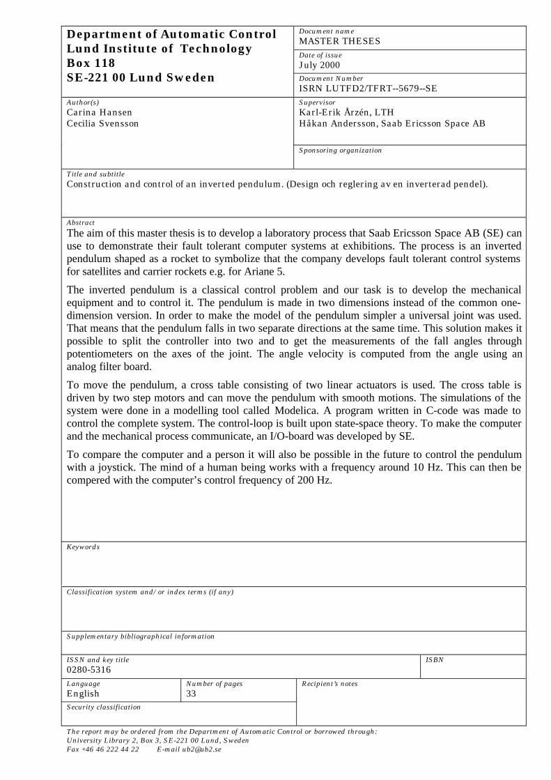
Abstract

The aim of this master thesis is to develop a laboratory process that Saab Ericsson Space AB (SE) canuse to demonstrate their fault tolerant computer systems at exhibitions. The process is an invertedpendulum shaped as a rocket to symbolize that the company develops fault tolerant control systemsfor satellites and carrier rockets e.g. for Ariane 5.

The inverted pendulum is a classical control problem and our task is to develop the mechanicalequipment and to control it. The pendulum is made in two dimensions instead of the common one-dimension version. In order to make the model of the pendulum simpler a universal joint was used.That means that the pendulum falls in two separate directions at the same time. This solution makes itpossible to split the controller into two and to get the measurements of the fall angles throughpotentiometers on the axes of the joint. The angle velocity is computed from the angle using ananalog filter board.

To move the pendulum, a cross table consisting of two linear actuators is used. The cross table isdriven by two step motors and can move the pendulum with smooth motions. The simulations of thesystem were done in a modelling tool called Modelica. A program written in C-code was made tocontrol the complete system. The control-loop is built upon state-space theory. To make the computerand the mechanical process communicate, an I/O-board was developed by SE.

To compare the computer and a person it will also be possible in the future to control the pendulumwith a joystick. The mind of a human being works with a frequency around 10 Hz. This can then becompered with the computer’s control frequency of 200 Hz.

Keywords

Classification system and/or index terms (if any)

Supplementary bibliographical information

ISSN and key title0280-5316

ISBN

LanguageEnglish

Number of pages33

Security classification

Recipient’s notes

The report may be ordered from the Department of Automatic Control or borrowed through:University Library 2, Box 3, SE-221 00 Lund, SwedenFax +46 46 222 44 22 E-mail [email protected]

Master Thesis Construction and control of an inverted pendulum 2000-06-20

2

Outline

• Introduction The first chapter presents the problem and goal of this master thesisand gives the background to what Saab Ericsson Space will use the equipment for.

• The Equipment Chapter 2 brings up the physical equipment to discussion. How thependulum should be built and which motor that is to prefer, are examples ofquestions answered in this part. The communication between the equipment and thecomputer is also described.

• Simulation The modelling and simulation is treated in Chapter 3. Force analysisand system equations are derived and the simulation tool is presented. The resultsare explained and conclusions are made for demands upon the equipment.

• Control Design In Chapter 4 the state-space controller is derived and comparedwith the PD-controller used in the simulation.

• Real-Time Implementation Here is an overview of the program and modulespresented. The computer hardware is also described.


3

Acknowledgements

We would like to thank Niclas Åberg at Östergrens Elmotor AB for untiring answeredall our questions about motors and linear actuators. We also want to thank ChristerHoubaer at Elwia for helping us finding a joystick that matches our demand for thependulum.

Thanks to section DD and DP for your support and for listen to our whining. Finally wewill thank our supervisors Karl-Erik Årzen at the Department of Automatic Control,Lund Institute of Technology, Håkan Andersson at Saab Ericsson Space AB.


4

Table of Contents

1. INTRODUCTION ..................................................................................................................................... 5

1.1 BACKGROUND ....................................................................................................................................... 51.2 PROBLEM DESCRIPTION......................................................................................................................... 51.3 OBJECTIVE ............................................................................................................................................. 51.4 STATUS .................................................................................................................................................. 5

2. PHYSICAL PROCESS DESCRIPTION................................................................................................ 6

2.1 THE PENDULUM..................................................................................................................................... 62.2 CROSS TABLE......................................................................................................................................... 8

2.2.1 Construction and Function ........................................................................................................112.3 MOTOR.................................................................................................................................................11

2.3.1 Step motor vs Servomotor..........................................................................................................112.3.2 Drive-unit....................................................................................................................................112.3.3 Limits for the step motor and the linear actuator ....................................................................12

2.4 BOARDS ...............................................................................................................................................13

3. MODELLING AND SIMULATION....................................................................................................14

3.1 MODELLING AN INVERTED PENDULUM ..............................................................................................14Force analysis and system equations ....................................................................................................14

3.2 MODELICA ...........................................................................................................................................163.2.1 Model and equation ...................................................................................................................17

3.3 RESULTS...............................................................................................................................................18

4. CONTROL DESIGN..............................................................................................................................22

4.1 CONTROL STRUCTURE.........................................................................................................................224.2 POLE-PLACEMENT...............................................................................................................................224.3 CALCULATION OF THE FEEDBACK VECTOR ........................................................................................234.4 PROCESS UNCERTAINTY......................................................................................................................24

5. PROGRAMMING ..................................................................................................................................25

5.1 STRUCTURE..........................................................................................................................................255.2 POLLING...............................................................................................................................................26

6. CONCLUSION ........................................................................................................................................28

7. ABBREVIATIONS..................................................................................................................................29

8. REFERENCES ........................................................................................................................................30

9. APPENDIX...............................................................................................................................................31

A JOYSTICKB LINEAR UNITC MOTORSD DRIVE-UNITE AVMF SCORPIOG MODELICAH PROGRAM


5

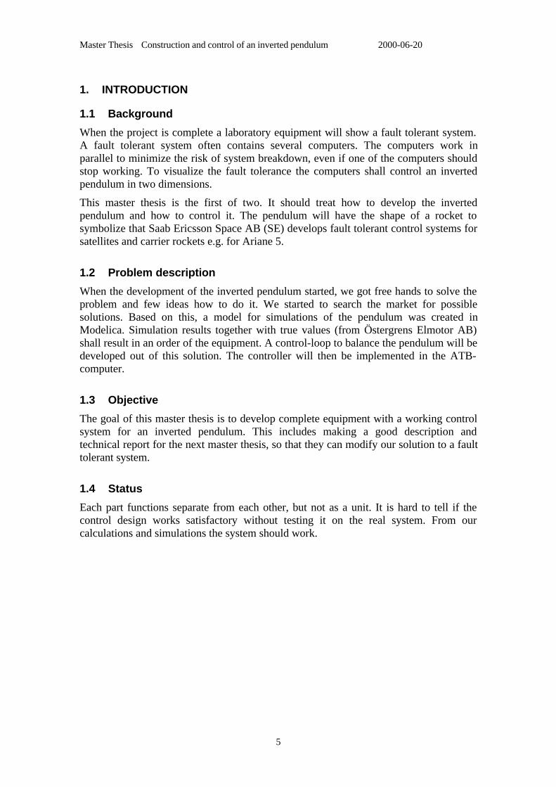
1. INTRODUCTION

1.1 Background

When the project is complete a laboratory equipment will show a fault tolerant system.A fault tolerant system often contains several computers. The computers work inparallel to minimize the risk of system breakdown, even if one of the computers shouldstop working. To visualize the fault tolerance the computers shall control an invertedpendulum in two dimensions.

This master thesis is the first of two. It should treat how to develop the invertedpendulum and how to control it. The pendulum will have the shape of a rocket tosymbolize that Saab Ericsson Space AB (SE) develops fault tolerant control systems forsatellites and carrier rockets e.g. for Ariane 5.

1.2 Problem description

When the development of the inverted pendulum started, we got free hands to solve theproblem and few ideas how to do it. We started to search the market for possiblesolutions. Based on this, a model for simulations of the pendulum was created inModelica. Simulation results together with true values (from Östergrens Elmotor AB)shall result in an order of the equipment. A control-loop to balance the pendulum will bedeveloped out of this solution. The controller will then be implemented in the ATB-computer.

1.3 Objective

The goal of this master thesis is to develop complete equipment with a working controlsystem for an inverted pendulum. This includes making a good description andtechnical report for the next master thesis, so that they can modify our solution to a faulttolerant system.

1.4 Status

Each part functions separate from each other, but not as a unit. It is hard to tell if thecontrol design works satisfactory without testing it on the real system. From ourcalculations and simulations the system should work.


6

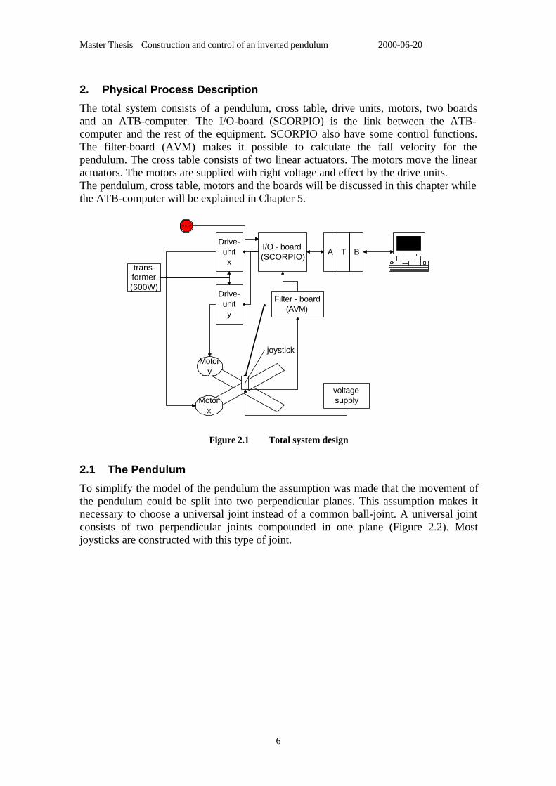
2. Physical Process Description

The total system consists of a pendulum, cross table, drive units, motors, two boardsand an ATB-computer. The I/O-board (SCORPIO) is the link between the ATB-computer and the rest of the equipment. SCORPIO also have some control functions.The filter-board (AVM) makes it possible to calculate the fall velocity for thependulum. The cross table consists of two linear actuators. The motors move the linearactuators. The motors are supplied with right voltage and effect by the drive units.The pendulum, cross table, motors and the boards will be discussed in this chapter whilethe ATB-computer will be explained in Chapter 5.

Motorx

Motory

Drive-unitx

STOP

joystick

I/O - board(SCORPIO)

A T B

Drive-unity

trans-former(600W)

voltagesupply

Filter - board(AVM)

Figure 2.1 Total system design

2.1 The Pendulum

To simplify the model of the pendulum the assumption was made that the movement ofthe pendulum could be split into two perpendicular planes. This assumption makes itnecessary to choose a universal joint instead of a common ball-joint. A universal jointconsists of two perpendicular joints compounded in one plane (Figure 2.2). Mostjoysticks are constructed with this type of joint.


7

Figure 2.2 Universal joint.

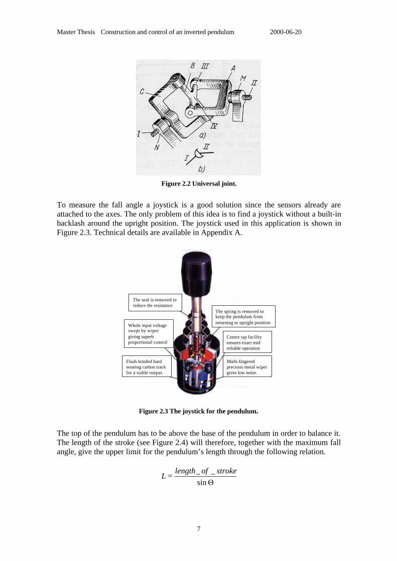
To measure the fall angle a joystick is a good solution since the sensors already areattached to the axes. The only problem of this idea is to find a joystick without a built-inbacklash around the upright position. The joystick used in this application is shown inFigure 2.3. Technical details are available in Appendix A.

Centre tap facilityensures exact midreliable operation

Multi-fingeredprecious metal wipergives low noise.

Flush bonded hardwearing carbon trackfor a stable output.

Whole input voltageswept by wipergiving superbproportional control

The seal is removed toreduce the resistance

The spring is removed tokeep the pendulum fromreturning to upright position

Figure 2.3 The joystick for the pendulum.

The top of the pendulum has to be above the base of the pendulum in order to balance it.The length of the stroke (see Figure 2.4) will therefore, together with the maximum fallangle, give the upper limit for the pendulum’s length through the following relation.

Θ=

sin__ strokeoflength

L


8

Choosing the total motion to a maximum of 75×75-cm gives a stroke-length atapproximately 37 cm. The maximum fall angle of the joystick is ±18° and this will limitthe length of the pendulum to 119 cm. This will be discussed later in the simulationpart; the pendulum length will also be much shorter for other reasons.

Θ

length of stroke

z

x

L

Figure 2.4 Length of stroke.

2.2 Cross table

The ideas of how to balance the pendulum were numerous and varying. Everythingfrom pneumatic control in different shapes to the final solution with linear actuators wasdiscussed.

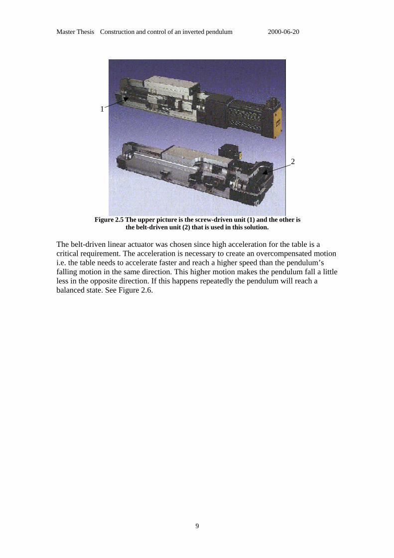
There are two available linear actuators one with belt-driven unit and the other withball-screw-driven unit, Figure 2.5. The belt-driven unit can reach higher speed,acceleration and a greater distance. The ball-screw-driven unit has higher repeatabilitybut can not reach as high acceleration as the belt-driven unit.

Design constraints for the pendulum:Max fall angle = 18°Max angle velocity ~ 2.6 rad/s ~ 149°/sMax length = 1.19 m


9

Figure 2.5 The upper picture is the screw-driven unit (1) and the other isthe belt-driven unit (2) that is used in this solution.

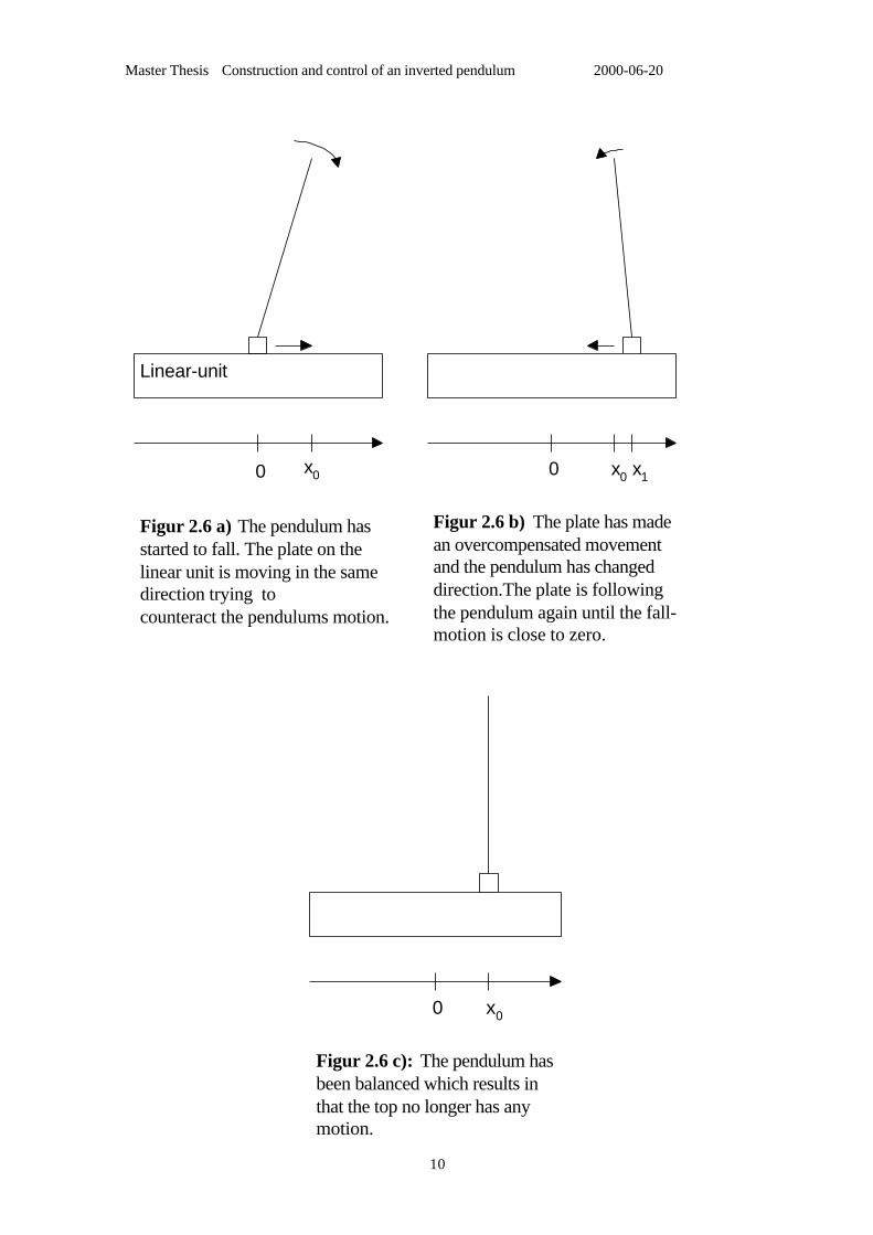
The belt-driven linear actuator was chosen since high acceleration for the table is acritical requirement. The acceleration is necessary to create an overcompensated motioni.e. the table needs to accelerate faster and reach a higher speed than the pendulum’sfalling motion in the same direction. This higher motion makes the pendulum fall a littleless in the opposite direction. If this happens repeatedly the pendulum will reach abalanced state. See Figure 2.6.

1

2


10

0 x0 0 x0 x1

Linear-unit

Figur 2.6 a) The pendulum hasstarted to fall. The plate on thelinear unit is moving in the samedirection trying tocounteract the pendulums motion.

Figur 2.6 b) The plate has madean overcompensated movementand the pendulum has changeddirection.The plate is followingthe pendulum again until the fall-motion is close to zero.

0 x0

Figur 2.6 c): The pendulum hasbeen balanced which results inthat the top no longer has anymotion.


11

2.2.1 Construction and Function

To create a two-dimension motion two linear actuators have to be mounted on top ofeach other in a cross shape. The moving part of the actuator is only a small plate on topof the unit. The bottom unit has to be more robust and it has to be driven by a strongermotor to bear the weight of the upper unit (see Appendix B). Each axle has its ownmotor and drive-unit so they are controlled separately from each other.

To check that the plate has not come to close to any edge there are four sensors on thetable, one sensor at each edge. When a sensor is set there are only two centimetres leftto the edge. The motor then has to be stopped before it hits the edge and becomeoverheated. To control if the plate on the cross table is centred in the middle of thetable, there are two centre sensors applied to the middle. The home sensors are set whenthe plate is in the exact right position. This is necessary since dead reckoning is used.More about the sensor use is discussed in the I/O-part, see Chapter1.4.

2.3 Motor

There are a lot of motors to choose among which all reach the demand of speed andrepeatability. The two motors discussed in the following chapter are common, and usedin many applications. They also have the advantage of being easy to control.

2.3.1 Step motor vs. Servomotor

Servo motorWith a servomotor it is possible to control position, number of revolutions and thebraking. By using higher frequencies compared to the step motor, high acceleration isachieved. A change of current direction will only affect the acceleration of the motor,not the direction of the motion. In this case, a feedback signal of velocity and position tocontrol the motor is needed. To get this feedback a sensor is used on the motor, makingit more expensive and complicated compared to a simple step motor.

Step motorThe step motor consists of one stator and one rotor. When one or more of the windingshave current drift, a magnetic field is generated. This field will turn the rotor untilbalance arises. The motor has now taken one step and found its new position. Bysending in pulses to the motor, the current drift will move from one winding to the next.This results in the rotor moving step by step, one at a time.

To change the motor’s speed or direction, the pulse frequency or the direction signal tothe drive-unit that controls the motor is changed. The motor can only take a step if apulse has been sent into it. This makes the motor easy to control since no feedbacksignals are needed as e.g. for the servomotor. The step motor was chosen for thisapplication due to the easy control and the low cost. (Appendix C)

2.3.2 Drive-unit

This is a high-performance motion control equipment, capable of producing rapidmovement and very high forces. It can be powered by 48Vdc or 70Vac and 5A supplies(appendix D). The pulse train and direction signal for the driver will come from theSCORPIO. The driver then creates the corresponding electrical pulse train to the motor.


12

2.3.3 Limits for the step motor and the linear actuator

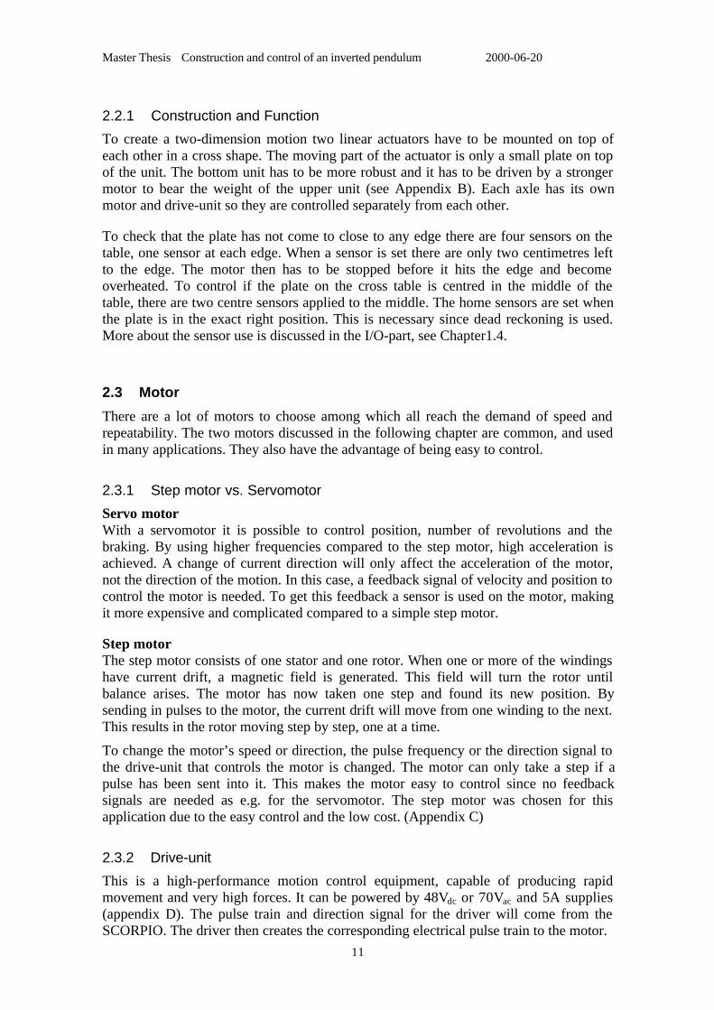
In the simulations (Chapter 3.3) it was found that the max velocity needed is 0.6 m/s, tostabilise the pendulum when the fall angle is large (~18°). The max velocity is reachedin 4 cm and has a linear progress as seen in figure 2.7. In the drive-unit it is possible tochange the step length for the motor. The step length is depending on how exact themovements have to be. In this case it does not have to be so exact. It is high velocitythat is needed. The lead on the linear unit has a circumference of 70mm for the smallunit and 100 mm for the large unit.

revolutionstepncecircumfereleadlinear

lengthStep/

___ =

step/revolution 400 800 2000 4000Step length x (mm) 0.1750 0.0875 0.0335 0.0175Step length y (mm) 0.2500 0.1250 0.0500 0.0250Table 2.1: Step length

The reach the same velocity with a shorter step length SCORPIO has to send out pulseswith higher frequencies to the motors. That can cause disturbances that are not wanted.The lowest precision, 400 step/revolution, is therefore chosen.

(m)

(m/s) Max velocity0.6 (m/s)0.6

0.2

0.02 0.04

0.4

Figure 2.7 Acceleration from 0 to 0.6 in 4 cm.

Based on this, some important values can be calculated.

Limits for the actuator:Position = 0.37 mMax velocity = 0.6 m/sMax acceleration = 4.5 m/s2


13

The connections to the motor must be using a high quality braided-screen cable. This toprevent cross talk disturbances between control signals.

2.4 Boards

To control the step motor drivers a specified I/O board, called SCORPIO, has beendeveloped by SE. It interfaces the signals from four end-sensors and two centre-sensors.It also takes care of all the signals coming from the inverted pendulum. The anglesignals are conditioned to provide a better measurement and filtered to provide the anglevelocity. The filter board (AVM) is developed by LTH (Department of AutomaticControl). Specifications for this board are found in Appendix E. These signals areconnected to an A/D-converter on SCORPIO.

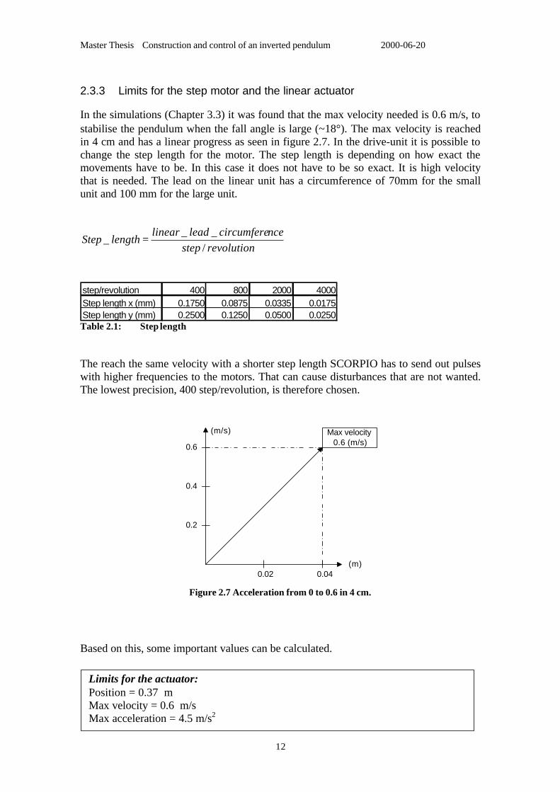
SCORPIO should also count all steps that have been sent out, making it possible toupdate the position counting and velocity of the table in the program. The properties ofthe counter are seen in Figure 2.8. Every time the pendulum passes the center sensor thecounter is reset and restarted. Signals from the program out to SCORPIO determine howmany steps the motors should move and in which direction. If the counter passes thelimit an overflow/underflow bit is set. This bit will not be cleared until the plate passesthe center sensor. The specification of SCORPIO is found in Appendix F.

counted area

y

x

overflow x,y

underflow xoverflow yunderflow x,y

overflow xunderflow y

TotalTableArea

Figure 2.8 Count area on the cross table.

Limits for the motor:Step length x = 0.175 mmStep length y = 0.250 mmSample time = 4.992 msecMax number of steps per sample (x-direction) = 17 step/sampleMax number of steps per sample (y-direction) = 12 step/sampleSample to reach max velocity = 0.13 / 4.99m = 26 samples


14

3. Modelling and Simulation

A model of the equipment is used for the control design for the real system. Thedynamics of the model is calculated to be as close as possible to the real process.Through simulations it is possible to extract the requirements for the equipment such asthe length of the pendulum and requirements upon the velocity and acceleration of thetable. Also the impact of noise and sample rates on the measurements and stability ofthe system is studied.

3.1 Modelling an inverted pendulum

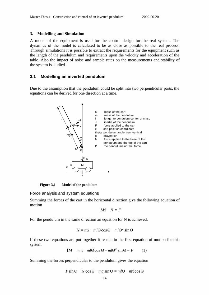
Due to the assumption that the pendulum could be split into two perpendicular parts, theequations can be derived for one direction at a time.

M mass of the cartm mass of the penduluml length to pendulum center of massJ inertia of the pendulumF force applied to the cartx cart position coordinatetheta pendulum angle from verticalg gravitationN force applied to the base of the pendulum and the top of the cartP the pendulums normal force

MF

x

NPΘl

l

mg

Jθ

x

N P

Figure 3.1 Model of the pendulum

Force analysis and system equations

Summing the forces of the cart in the horizontal direction give the following equation ofmotion

FNxM =+&&

For the pendulum in the same direction an equation for N is achieved.

ΘΘ−ΘΘ+= sincos 2&&&&& mlmlxmN

If these two equations are put together it results in the first equation of motion for thissystem.

( ) FmlmlxmM =ΘΘ−ΘΘ++ sincos 2&&&&& (1)

Summing the forces perpendicular to the pendulum gives the equation

Θ+Θ=Θ−Θ+Θ cossincossin xmmlmgNP &&&&


15

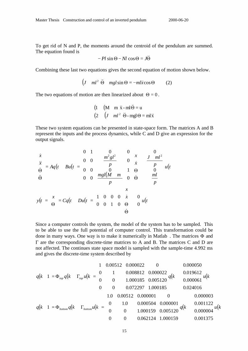
To get rid of N and P, the moments around the centroid of the pendulum are summed.The equation found is

Θ=Θ−Θ− &&JNlPl cossin

Combining these last two equations gives the second equation of motion shown below.

( ) Θ−=Θ+Θ+ cossin2 xmlmglmlJ &&&& (2)

The two equations of motion are then linearized about 0=Θ .

( ) ( )( ) ( ) xmlmgl-2

uml-xmM12 &&&&

&&&&

=ΘΘ+

=Θ+

mlJ

These two system equations can be presented in state-space form. The matrices A and Brepresent the inputs and the process dynamics, while C and D give an expression for theoutput signals.

( ) ( )( )

( )tu

pml

pmlJ

xx

pmMmgl

pglm

tButAqxx

+

+

ΘΘ

+

=+=

ΘΘ 0

0

000

1000

000

0010222

&

&

&&&&&&

( ) ( ) ( ) ( )tuxx

tDutCqx

ty

+

ΘΘ

=+=

Θ

=00

01000001

&

&

Since a computer controls the system, the model of the system has to be sampled. Thisto be able to use the full potential of computer control. This transformation could bedone in many ways. One way is to make it numerically in Matlab. The matrices Φ andΓ are the corresponding discrete-time matrices to A and B. The matrices C and D arenot affected. The continues state space model is sampled with the sample-time 4.992 msand gives the discrete-time system described by

( ) ( ) ( ) ( ) ( )

( ) ( ) ( ) ( ) ( )kukqkukqkq

kukqkukqkq

bottombottom

toptop

+

=Γ+Φ=+

+

=Γ+Φ=+

001375.0000004.0001122.0000003.0

000159.1062124.000005120.0000159.100000001.0000504.00.10

0000001.000512.00.1

1

024016.0000061.0019612.0000050.0

000185.1072297.000005120.0000185.100000022.0008812.010

0000022.000512.01

1


16

3.2 Modelica

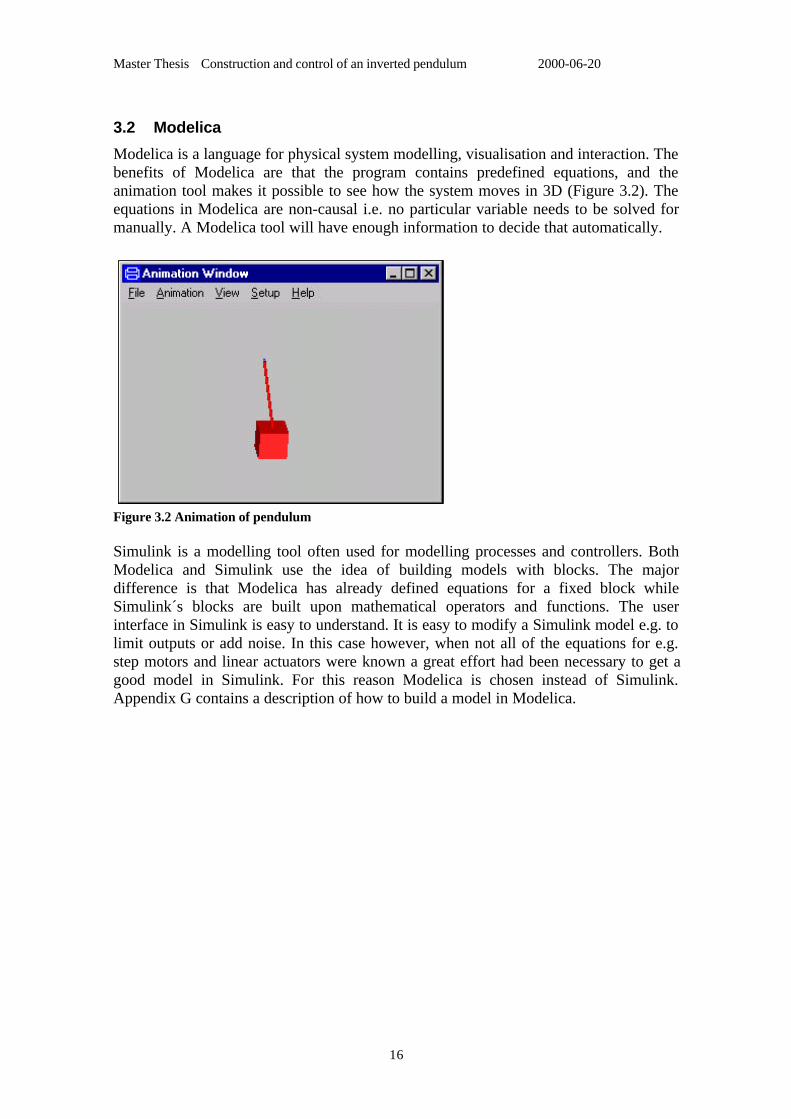
Modelica is a language for physical system modelling, visualisation and interaction. Thebenefits of Modelica are that the program contains predefined equations, and theanimation tool makes it possible to see how the system moves in 3D (Figure 3.2). Theequations in Modelica are non-causal i.e. no particular variable needs to be solved formanually. A Modelica tool will have enough information to decide that automatically.

Figure 3.2 Animation of pendulum

Simulink is a modelling tool often used for modelling processes and controllers. BothModelica and Simulink use the idea of building models with blocks. The majordifference is that Modelica has already defined equations for a fixed block whileSimulink´s blocks are built upon mathematical operators and functions. The userinterface in Simulink is easy to understand. It is easy to modify a Simulink model e.g. tolimit outputs or add noise. In this case however, when not all of the equations for e.g.step motors and linear actuators were known a great effort had been necessary to get agood model in Simulink. For this reason Modelica is chosen instead of Simulink.Appendix G contains a description of how to build a model in Modelica.


17

3.2.1 Model and equation

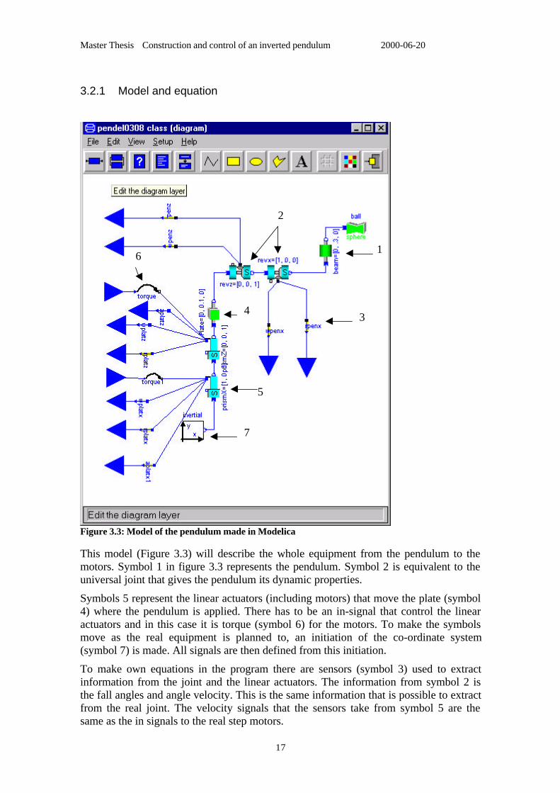
Figure 3.3: Model of the pendulum made in Modelica

This model (Figure 3.3) will describe the whole equipment from the pendulum to themotors. Symbol 1 in figure 3.3 represents the pendulum. Symbol 2 is equivalent to theuniversal joint that gives the pendulum its dynamic properties.

Symbols 5 represent the linear actuators (including motors) that move the plate (symbol4) where the pendulum is applied. There has to be an in-signal that control the linearactuators and in this case it is torque (symbol 6) for the motors. To make the symbolsmove as the real equipment is planned to, an initiation of the co-ordinate system(symbol 7) is made. All signals are then defined from this initiation.

To make own equations in the program there are sensors (symbol 3) used to extractinformation from the joint and the linear actuators. The information from symbol 2 isthe fall angles and angle velocity. This is the same information that is possible to extractfrom the real joint. The velocity signals that the sensors take from symbol 5 are thesame as the in signals to the real step motors.

1

2

34

5

7

6


18

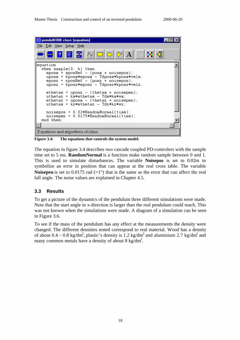
Figure 3.4: The equations that controls the system model.

The equation in figure 3.4 describes two cascade coupled PD-controlers with the sampletime set to 5 ms. RandomNormal is a function make random sample between 0 and 1.This is used to simulate disturbances. The variable Noisepos is set to 0.02m tosymbolize an error in position that can appear at the real cross table. The variableNoisepen is set to 0.0175 rad (=1°) that is the same as the error that can affect the realfall angle. The noise values are explained in Chapter 4.5.

3.3 Results

To get a picture of the dynamics of the pendulum three different simulations were made.Note that the start angle in x-direction is larger than the real pendulum could reach. Thiswas not known when the simulations were made. A diagram of a simulation can be seenin Figure 3.6.

To see if the mass of the pendulum has any effect at the measurements the density werechanged. The different densities tested correspond to real material. Wood has a densityof about 0.4 – 0.8 kg/dm3, plastic’s density is 1.2 kg/dm3 and aluminium 2.7 kg/dm3 andmany common metals have a density of about 8 kg/dm3.


19

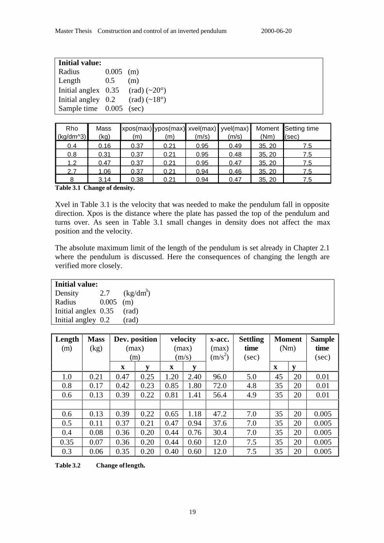
Initial value:Radius 0.005 (m)Length 0.5 (m)Initial anglex 0.35 (rad) (~20°)Initial angley 0.2 (rad) (~18°)Sample time 0.005 (sec)

Rho Mass xpos(max) ypos(max) xvel(max) yvel(max) Moment Setting time(kg/dm^3) (kg) (m) (m) (m/s) (m/s) (Nm) (sec)

0.4 0.16 0.37 0.21 0.95 0.49 35, 20 7.50.8 0.31 0.37 0.21 0.95 0.48 35, 20 7.51.2 0.47 0.37 0.21 0.95 0.47 35, 20 7.52.7 1.06 0.37 0.21 0.94 0.46 35, 20 7.58 3.14 0.38 0.21 0.94 0.47 35, 20 7.5

Table 3.1 Change of density.

Xvel in Table 3.1 is the velocity that was needed to make the pendulum fall in oppositedirection. Xpos is the distance where the plate has passed the top of the pendulum andturns over. As seen in Table 3.1 small changes in density does not affect the maxposition and the velocity.

The absolute maximum limit of the length of the pendulum is set already in Chapter 2.1where the pendulum is discussed. Here the consequences of changing the length areverified more closely.

Initial value:Density 2.7 (kg/dm3)Radius 0.005 (m)Initial anglex 0.35 (rad)Initial angley 0.2 (rad)

Dev. position(max)(m)

velocity(max)(m/s)

Moment(Nm)

Length(m)

Mass(kg)

x y x y

x-acc.(max)(m/s2)

Settlingtime(sec)

x y

Sampletime(sec)

1.0 0.21 0.47 0.25 1.20 2.40 96.0 5.0 45 20 0.010.8 0.17 0.42 0.23 0.85 1.80 72.0 4.8 35 20 0.010.6 0.13 0.39 0.22 0.81 1.41 56.4 4.9 35 20 0.01

0.6 0.13 0.39 0.22 0.65 1.18 47.2 7.0 35 20 0.0050.5 0.11 0.37 0.21 0.47 0.94 37.6 7.0 35 20 0.0050.4 0.08 0.36 0.20 0.44 0.76 30.4 7.0 35 20 0.0050.35 0.07 0.36 0.20 0.44 0.60 12.0 7.5 35 20 0.0050.3 0.06 0.35 0.20 0.40 0.60 12.0 7.5 35 20 0.005

Table 3.2 Change of length.


20

A small fall angle will give a shorter turning point than a larger fall angle. That explainsthe big difference between the maximum movement in x-direction and y-directionrespectively. Since the max deviation of the real pendulum is 18° the conclusions for theequipment was drawn from the x-direction simulation.

To keep the table size down the length of the pendulum was reduced as seen in crossTable 3.2. Between 0.3 m and 0.6 m the difference in position deviation is not verylarge. The table size will be about 0.75 m. The corresponding velocity is of vitalimportance to decide which length to use. A length of 0.3 m only requires a velocity of0.6 m/s while a length of 0.6 m requires 1.18 m/s. Choosing the shorter pendulummakes it possible to use step motors. The physical limits of the motor are found inChapter 2.3.

Even if the shorter pendulum implies both lower velocity and acceleration, theaccelerations are still very high. A simulation with a bounded acceleration should bepreferred but problems modifying the Modelica model made that impossible. Insteadsome assumptions were made.

The fall angle will never reach its maximum. A smaller angle gives a smaller positiondeviation. This gives some extra space and time to counteract the falling motion of thependulum making it possible to balance the pendulum with a limited acceleration.

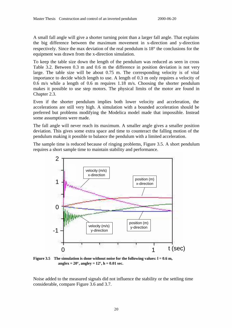
The sample time is reduced because of ringing problems, Figure 3.5. A short pendulumrequires a short sample time to maintain stability and performance.

2

1

-1

0

0 1 t (sec)

velocity (m/s)x-direction

velocity (m/s)y-direction

position (m)x-direction

position (m)y-direction

Figure 3.5 The simulation is done without noise for the following values: l = 0.6 m,anglex = 20°, angley = 12°, h = 0.01 sec.

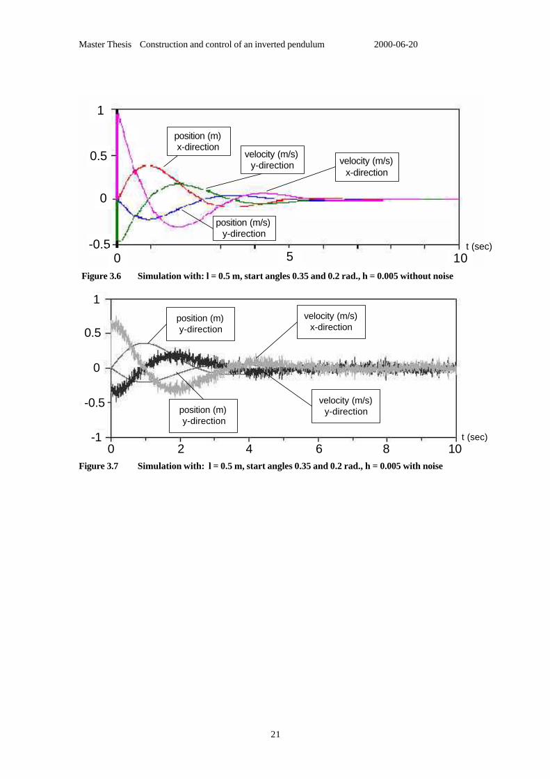
Noise added to the measured signals did not influence the stability or the settling timeconsiderable, compare Figure 3.6 and 3.7.


21


velocity (m/s)y-direction

position (m)x-direction

position (m/s)y-direction

1

0.5

-0.55

0

0 10t (sec)

Figure 3.6 Simulation with: l = 0.5 m, start angles 0.35 and 0.2 rad., h = 0.005 without noise

1

0.5

0

-0.5

-10 2 4 6 8 10


velocity (m/s)y-directionposition (m)

y-direction

position (m)y-direction

t (sec)

Figure 3.7 Simulation with: l = 0.5 m, start angles 0.35 and 0.2 rad., h = 0.005 with noise


22

4. Control Design

Modelling the dynamic properties of a process makes it possible to calculate a controllerfor the process. Sometimes process uncertainty, disturbances and time delays have to betaken into account. However as shown later this controller does not have to involvethese problems.

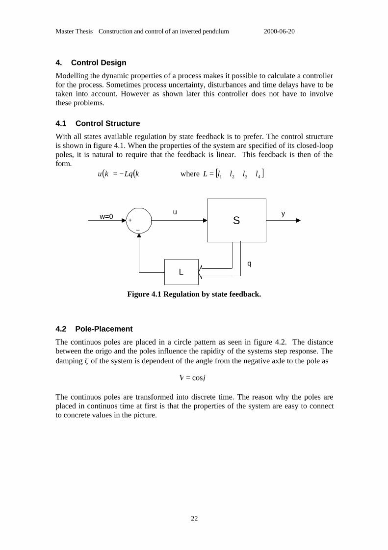
4.1 Control Structure

With all states available regulation by state feedback is to prefer. The control structureis shown in figure 4.1. When the properties of the system are specified of its closed-looppoles, it is natural to require that the feedback is linear. This feedback is then of theform.

( ) ( )kLqku −= where [ ]4321 llllL =

S+ _

L

y

q

uw=0

Figure 4.1 Regulation by state feedback.

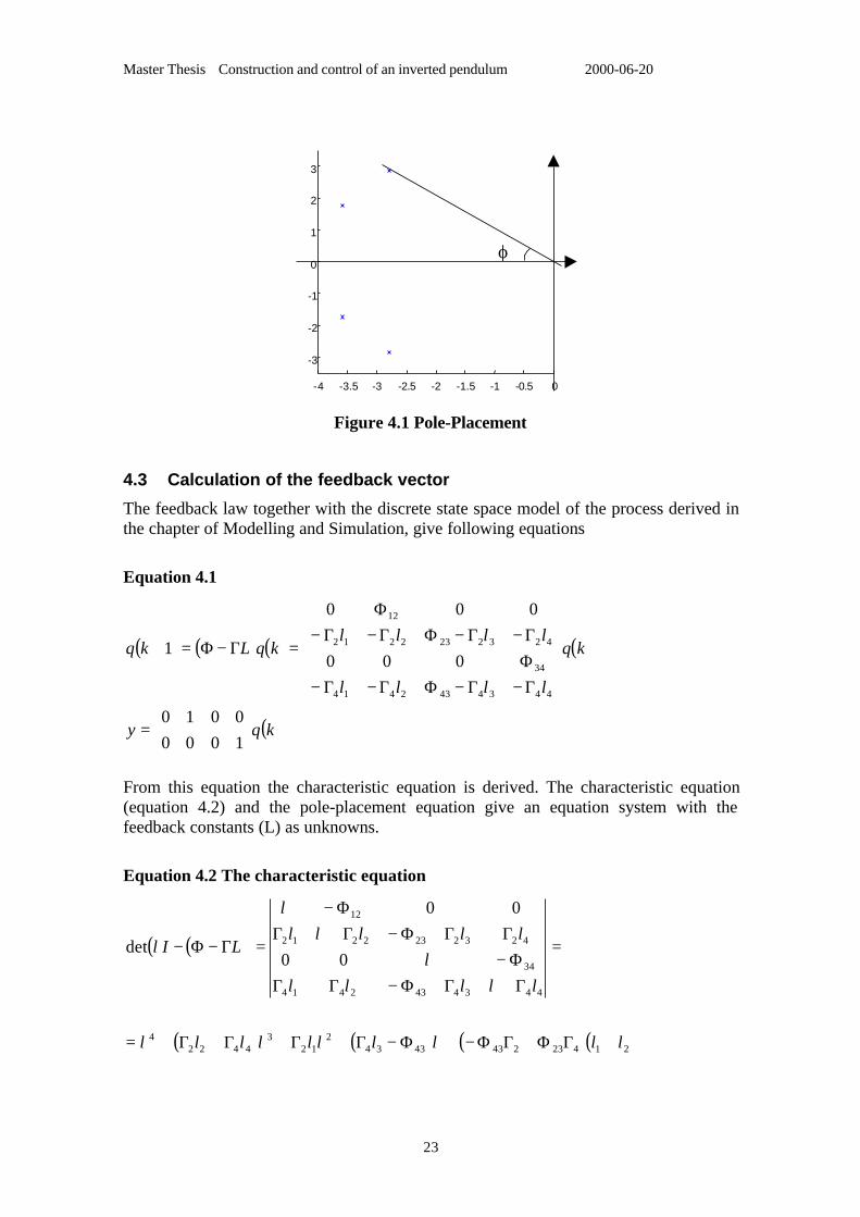
4.2 Pole-Placement

The continuos poles are placed in a circle pattern as seen in figure 4.2. The distancebetween the origo and the poles influence the rapidity of the systems step response. Thedamping ζ of the system is dependent of the angle from the negative axle to the pole as

ϕς cos=

The continuos poles are transformed into discrete time. The reason why the poles areplaced in continuos time at first is that the properties of the system are easy to connectto concrete values in the picture.


23

-4 -3.5 -3 -2.5 -2 -1.5 -1 -0.5 0

-3

-2

-1

0

1

2

3

ϕ

Figure 4.1 Pole-Placement

4.3 Calculation of the feedback vector

The feedback law together with the discrete state space model of the process derived inthe chapter of Modelling and Simulation, give following equations

Equation 4.1

( ) ( ) ( ) ( )

( )kqy

kq

llll

llllkqLkq

=

Γ−Γ−ΦΓ−Γ−ΦΓ−Γ−ΦΓ−Γ−

Φ

=Γ−Φ=+

10000010

000

000

1

4434432414

34

4232232212

12

From this equation the characteristic equation is derived. The characteristic equation(equation 4.2) and the pole-placement equation give an equation system with thefeedback constants (L) as unknowns.

Equation 4.2 The characteristic equation

( )( )

( ) ( ) ( )( )2142324343342

123

44224

4434432414

34

4232232212

12

00

00

det

llllll

llll

llllLI

+ΓΦ+ΓΦ−+Φ−Γ+Γ+Γ+Γ+=

=

Γ+Γ+Φ−ΓΓΦ−

ΓΓ+Φ−Γ+ΓΦ−

=Γ−Φ−

λλλλ

λλ

λλ

λ


24

4.4 Process uncertainty

The A/D-converter on SCORPIO needs 10µs to sample and place the measurementsinto the registers in the ATB. Measuring the calculation time in the program give aworst case of 18.75µs. These two delays added to the delay to set out the control signalgives a total delay of 29µs. The delay is then about 0.58 % of the sample time and doesnot need to be taken into consideration.

Many different sources can contribute to the total error in the angle measurement. Thevoltage supplies over the potentiometers in the joystick e.g. can variate. To prevent thisa reference generator is used. The reference is placed on the AVM. The signals from thejoystick pass through the AVM can be affected by disturbances. These disturbances arereduced to about 100mV through screened cables. The value 100mV corresponds toabout 0.396°. The truncation error that appears in the A/D-converter is 0.154°. If thependulum fall with a velocity of 149°/s and the time delay is 29µs a angle error of0.004° arise. The total angle error is 0.55°. The simulations managed an error of 1°,which is nearly twice the calculated error.

The mass of the pendulum does not influence the control as seen in the simulations.However, the mass matters when the pendulum changes direction. The breakout frictionis easier overcome with a heavy pendulum.

The repeatability was of minor importance compared to the velocity in the choice oflinear unit. To prevent errors in the control calculations a function in the programadjusts the position (chapter 5.1). In the simulations the control has been successful withan error of 2cm in position. With a step length of 0.25 mm, this results in a maximumerror of up to 80 steps without disturbing the control.


25

5. Programming

The program was edited in Borland C++ on a PC with NT-platform and compiled by afree GCC (gnu c-compiler) in UNIX-environment. The choice of language is based onthe environment of the ATB-computer. The ATB, computer is part of a fault tolerantcomputer system designed by SE. The ATB was used to demonstrate the fault tolerantcomputer concept for the Automatic Transfer Vehicle (ATV), in the frame of theInternational Space Station (ISS). The ATB is based on an ERC32, a 32-bits Sparcprocessor, specifically designed for space applications. The processor ERC32 makes itpossible to use C or ADA. C has been chosen since it is easier and faster to learn.

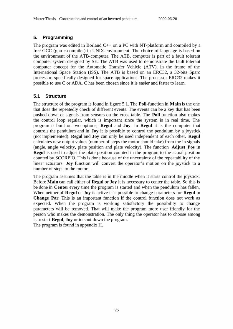
5.1 Structure

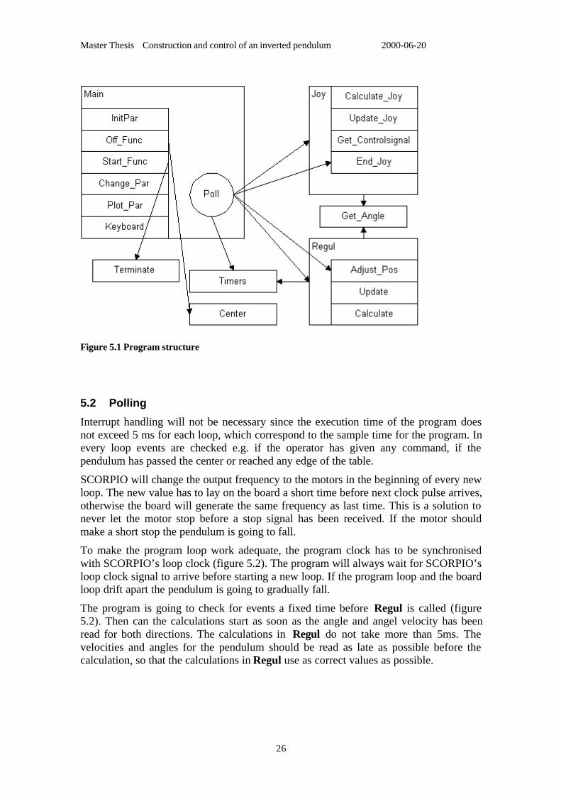
The structure of the program is found in figure 5.1. The Poll-function in Main is the onethat does the repeatedly check of different events. The events can be a key that has beenpushed down or signals from sensors on the cross table. The Poll-function also makesthe control loop regular, which is important since the system is in real time. Theprogram is built on two options, Regul and Joy. In Regul it is the computer thatcontrols the pendulum and in Joy it is possible to control the pendulum by a joystick(not implemented). Regul and Joy can only be used independent of each other. Regulcalculates new output values (number of steps the motor should take) from the in signals(angle, angle velocity, plate position and plate velocity). The function Adjust_Pos inRegul is used to adjust the plate position counted in the program to the actual positioncounted by SCORPIO. This is done because of the uncertainty of the repeatability of thelinear actuators. Joy function will convert the operator’s motion on the joystick to anumber of steps to the motors.

The program assumes that the table is in the middle when it starts control the joystick.Before Main can call either of Regul or Joy it is necessary to center the table. So this isbe done in Center every time the program is started and when the pendulum has fallen.When neither of Regul or Joy is active it is possible to change parameters for Regul inChange_Par. This is an important function if the control function does not work asexpected. When the program is working satisfactory the possibility to changeparameters will be removed. That will make the program more user friendly for theperson who makes the demonstration. The only thing the operator has to choose amongis to start Regul, Joy or to shut down the program.The program is found in appendix H.


26

Figure 5.1 Program structure

5.2 Polling

Interrupt handling will not be necessary since the execution time of the program doesnot exceed 5 ms for each loop, which correspond to the sample time for the program. Inevery loop events are checked e.g. if the operator has given any command, if thependulum has passed the center or reached any edge of the table.

SCORPIO will change the output frequency to the motors in the beginning of every newloop. The new value has to lay on the board a short time before next clock pulse arrives,otherwise the board will generate the same frequency as last time. This is a solution tonever let the motor stop before a stop signal has been received. If the motor shouldmake a short stop the pendulum is going to fall.

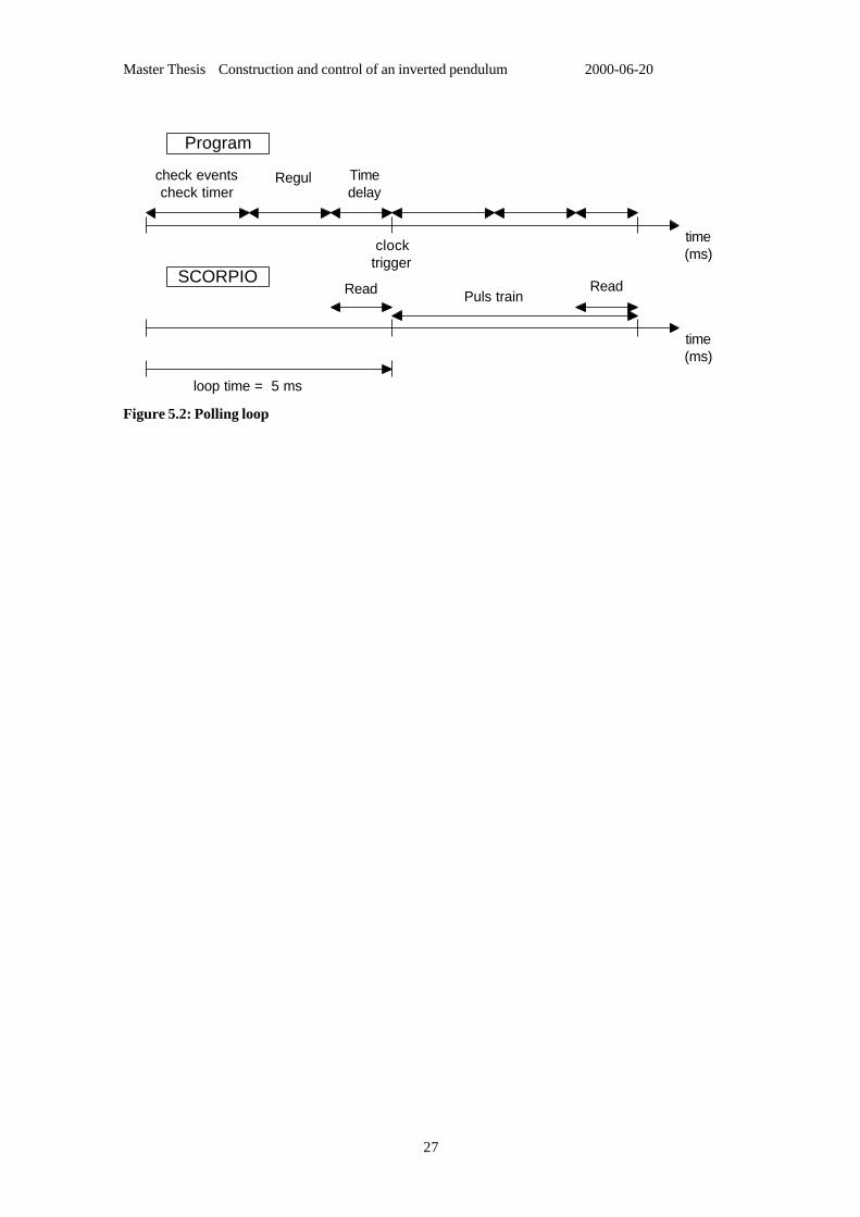
To make the program loop work adequate, the program clock has to be synchronisedwith SCORPIO’s loop clock (figure 5.2). The program will always wait for SCORPIO’sloop clock signal to arrive before starting a new loop. If the program loop and the boardloop drift apart the pendulum is going to gradually fall.

The program is going to check for events a fixed time before Regul is called (figure5.2). Then can the calculations start as soon as the angle and angel velocity has beenread for both directions. The calculations in Regul do not take more than 5ms. Thevelocities and angles for the pendulum should be read as late as possible before thecalculation, so that the calculations in Regul use as correct values as possible.


27

loop time = 5 ms

Program

SCORPIO

clocktrigger

check eventscheck timer

Regul Timedelay

Read Puls trainRead

time(ms)

time(ms)

Figure 5.2: Polling loop


28

6. Conclusion

The main goal with this master thesis was to develop an equipment from specification toa final commission. The total system is not finished because of delays in delivering ofthe mechanical equipment and problems with the development of SCORPIO.

At this date all the parts of the system are working separately. The simulations havegiven the demands of the equipment. Modelica has been chosen to simulate the systemsince e.g. the step motor is very difficult to make model of in Simulink. To simplify thecalculations and simulations a universal joint has been chosen instead of a ball joint. Aball joint can be affected by a torque in contrast to the universal joint. That makes themodel equations for the ball joint very complicated. The AVM gives out the angle andangle velocity from the pendulum with very little noise. The estimated total noise andtime delay lay within the limits.

So the only things that remains are to put all parts together and do the final tests and fineadjustments.


29

7. Abbreviations

ATB Avionia Test Bench

ATV Automatic Transfer Vehicle

AVM Angle and Velocity Measurements

ISS International Space Station

LTH Lund Institute of Technology

SCORPIO Step motor Controller and Rocket Position IO board

SE Saab Ericsson Space (AB)

e.g for example (Latin: exempli gratia)

i.e that is (Latin: id est)

vs. versus

Ariane 5 Carrier rocket


30

8. REFERENCES

Karl J. Åström, Björn Wittenmark; Computer-Controlled Systems, Prentice Hall, 1997.

Ulf Bilting, Jan Skansholm; Vägen till C, Studentlitteratur, 1987.

L.J. Meriam, L.G. Kraige; Engineering Mechanics, Wiley, 1993.

Department of industrial electrical engineering and automation; Elmaskinsystem, 1997.

Östergrens Elmotor AB; Produktkatolog 2000.

Modelica; http://www.dynasim.se, http://www.simulink.org

Bill Messner, Dawn Tilbury, http://tech.buffalostate.edu/ctm/index.html, 1996.


31

9. Appendix.

A Joystick

B Linear unit

C Motors

D Drive-unit

E AVM

F SCORPIO

G Modelica

H Program

Documents

Construction and Control of an Inverted Pendulumcontrol.lth.se/documents/2000/5679.pdf · Construction and Control of an Inverted Pendulum Carina Hansen ... This solution makes it