Constructing Tax Efficient Withdrawal Strategies for Retirees

Dr. James DiLellio, Dr. Dan Ostrov

Paper No. GCAR-A005 Category: Research Article

Working Paper SeriesCenter for Applied Research

February, 2018

Constructing Tax Efficient Withdrawal Strategies for Retirees ∗

November 6, 2017

Abstract

We construct an algorithm for United States retirees that computes individualized tax-efficient

annual withdrawals from IRAs/401(k)s, Roth IRAs/Roth 401(k)s, and taxable accounts. Our al-

gorithm applies a new approach that generates an individualized strategy that results in consistent

improvements over non-individualized withdrawal strategies currently advocated by financial insti-

tutions and academics. Among other results, we quantifiably demonstrate why retirees should avoid,

not seek, dividend producing stocks in their taxable accounts. Our model, which can work to optimize

either portfolio longevity or the bequest to an heir, accommodates many salient tax code features,

including dividends, different taxable lots, conversions, and required minimum distributions.

keywords: retirement income, tax efficiency, optimization

United States retirees generally have their stock1 invested in three types of accounts: 1) tax-

deferred accounts (TDAs) like traditional IRAs or traditional 401(k)s, 2) Roth IRAs or Roth 401(k)s,

∗The authors wish to thank Clemens Sialm and Sanjiv Das for reviewing the manuscript and making suggestions forimprovements.

1In this paper, the term “stock” will be shorthand for a portfolio of stocks that may include mutual funds, exchange-traded funds, as well as a variety of individual stocks.

1

and 3) taxable accounts. These three accounts are governed by significantly different tax rules,

especially in the case of the taxable account, that can be quite complicated. Much attention has been

given by non-academic institutions, as well as academic researchers, for how to best build up these

accounts in preparation for retirement. Brown et al. (2016), for example, provides a comprehensive

list of academic papers in this area. Intrinsic to answering this question, as well as of great interest

in its own right, is understanding the somewhat less investigated question of how to best withdraw

from these three accounts during retirement. The sequencing of withdrawals that a retiree makes

among stock accounts with varying tax structures can have a significant effect on their portfolio’s

longevity or, after the retiree passes away, on the size and utility of their bequest to an heir. In

this paper, we provide an algorithm that determines a strategy that is optimal or near-optimal for

allocating withdrawals among these three accounts, by minimizing the effect of taxes on the retiree

and the retiree’s heir.

Non-academic advice, coming from investment firms, financial advisors, and books on retirement,

recommend strategies for retirees’ withdrawal choices that are often far from optimal and often in

contradiction with each other, with the exception that there is general agreement that Required

Minimum Distributions (RMDs) should be taken from TDAs. For example, one very common

category of strategies, termed “naıve” strategies by Horan (2006a and 2006b), recommends that

retirees completely exhaust one account before moving to the next. The books by Solin (2010),

Rodgers (2009), and Lange (2009), suggest sequencing withdrawals so that retirees drain taxable

accounts first, then TDAs, and finally Roth accounts. This strategy is also endorsed by large

retail investment firms Fidelity (see Fidelity (2014) and Fidelity (2015)) and Vanguard (Vanguard

(2013)). In contrast, other financial authors, such as Larimore, Lindauer, Ferri, and Dogu (2011),

recommend first draining taxable accounts, but then recommend draining Roth accounts followed

finally by TDAs. Another Vanguard paper (Jaconetti and Bruno (2008)) recommends that the

2

decision on whether to drain the TDA or Roth account immediately following the taxable account

should be based on expected future marginal tax rates. Coopersmith and Sumutka (2011) estimate

the suboptimality of these naıve strategies to be approximately 16%. This agrees with DiLellio and

Ostrov (2017), who provide illustrations for which the naıve approaches are 10-26% suboptimal.

A second set of strategies, termed “informed” strategies by Horan (2006a and 2006b), use TDA

spending up to the top of a given tax bracket in every year. This is advocated in the book by Piper

(2013), who suggests filling any remaining consumption needs first with taxable stock, then with

Roth money, and lastly the TDA, if the TDA is not already exhausted. The informed strategies are

a considerable improvement over the naive strategies, but their inability to consider using the TDA

to partially fill a tax bracket or to consider using different amounts of TDA spending in different

years generally makes them suboptimal.

From an academic research point of view, there are two potential approaches to find the optimal

withdrawal strategy. The first, and seemingly most obvious, is to use one of the many numerical

methods available (see, for example, the book by Nocedal and Wright (2006)) to solve this constrained

optimization problem. However, to our knowledge there are no recent papers following this approach,

because, in practice, these numerical methods generally fail by producing a locally optimal strategy

that is far from the global optimum.

The second academic approach for locating the optimal withdrawal strategy, which this paper

among others takes, is to directly consider the implications of the tax laws and work to mini-

mize their downside for the retiree. Brown et al. (2016) points out that in the broader realm of

retirement-related academic research, “prior literature often...considers tax advantaged accounts in

an environment with a known, flat tax rate.” The flat tax rate assumption can be found, for example,

in Shoven and Sialm (2003) and Dammon et al. (2004), among many others. If the income tax rate

is flat, papers by Spitzer and Singh (2006) and Cook, Meyer, and Reichenstein (2015) in discrete

3

time, and by DiLellio and Ostrov (2017) in continuous time, give compelling examples and cases

that suggest the withdrawal strategy between the TDA and Roth account is irrelevant. In Appendix

1, we give a simple proof in continuous time that definitively shows the withdrawal strategy in this

flat tax environment does not matter. Even in the context of progressive tax brackets used in this

paper, this fact has important implications.

Within the context of withdrawal optimization for just TDA and Roth accounts, Horan’s (2006a

and 2006b) informed strategies, described previously, were a considerable step towards optimizing

a retiree’s portfolio longevity. This seminal work was expanded and investigated further in Re-

ichenstein, Horan, and Jennings (2012). Al Zaman (2008) extended a retiree’s possible objectives

to optimal bequests, in addition to the easier subcase of optimal portfolio longevity. DiLellio and

Ostrov (2017) give an algorithm that yields an optimal TDA and Roth account withdrawal strategy

for either the goal of optimizing bequests or the subcase of optimizing portfolio longevity. That

algorithm, summarized in Step 1.1 of Stage 1 in Subsection 4.3 of this paper, yields a geometrically

simple, easy to understand optimal strategy that becomes an important subroutine for this paper.

However, because taxable accounts have very different taxation rules than TDAs and Roth accounts,

this paper will require a far more complex algorithm, requiring a number of additional steps and

stages. Also, unlike DiLellio and Ostrov (2017), while the resulting withdrawal strategy in this pa-

per will often be optimal, to be computationally tractable, we allow some small assumptions and

approximations that will result in some cases where the resulting strategy will be near-optimal. We

will point out these assumptions and approximations when they occur.

Previous papers, such as Spitzer and Singh (2006), that consider how to optimize the longevity

of portfolios with TDAs, Roth accounts, and taxable stock accounts have proposed a variety of

fixed strategies and then compared their effectiveness for different financial scenarios. For example,

Sumutka, Sumutka, and Coopersmith (2012) compare the effectiveness of a wide variety of naıve

4

and informed withdrawal strategies for an array of portfolios. Cook, Meyer, and Reichenstein (2015)

cleverly expanded the field of possible strategies by considering the advantages of using conversions

from the TDA account in addition to withdrawals in a variety of examples. We address the potential

benefits these conversions can provide in Section 6.

Our approach differs from previous research in that it looks to construct a tax efficient strategy by

means of an adaptive algorithm that can tailor itself to a retiree’s specific circumstances. This allows

us to better address a far wider range of circumstances than comparing fixed strategies allows. We

have not found a circumstance under which either a naıve or an informed strategy produces better

results, meaning a higher bequest or a longer portfolio longevity, than our algorithm produces. Our

model includes working with Required Minimum Distributions (RMDs) for TDAs, as is the case with

most of the academic research above, but it also considers the less commonly considered effects of

working with stock dividends and conversions from the TDA account. The model also accommodates

working with different taxable lots within the taxable account, since, when selling taxable stock, it

is always optimal to select the lot containing stock purchased at the highest share price. We note

that our algorithm is general enough to accommodate many common changes to tax policies, such

as a change to the number of tax brackets or the marginal tax rates, should such changes occur at

a later date.

While the algorithm works to optimally determine how much a retiree should spend each year

from their TDA, Roth, and taxable stock accounts — that is, these are the three decision variables

to be determined each year — it also accommodates two other sources of income. Both of these

sources provide fixed amounts of money each year. The first source, which we will call L(t) in this

paper, because it will be geometrically represented in the lower part of our graphs, encompasses any

known (or projected) sources of money, other than the TDA account, that are subject to income

tax. These include earned income, some pensions, annuities bought with pre-tax money, and the

5

earnings from annuities bought with post-tax money. It also applies to the Social Security benefits

of some wealthy retirees, as discussed in DiLellio and Ostrov (2017). The second source, which we

will call U(t) in this paper, because it will geometrically be represented in the upper part of our

graphs, encompasses any known (or projected) sources of money that (a) have tax rates that are

independent of the retiree’s allocation decisions among the TDA, Roth, and taxable accounts, and

(b) unlike L(t), have no effect on the taxation rate of the TDA or taxable account. Examples include

tax-free gifts and tax-free accounts like Health Savings Accounts, some pensions, and the principal

from annuities bought with post-tax money. It also applies to the Social Security benefits of some

less well-off retirees, again as discussed in DiLellio and Ostrov (2017).

The main restriction in this paper is that nothing is stochastic. Everything in the future is

known or, more realistically, projected by the retiree and/or their financial advisor. This includes

the annual rate of return for the stock, the stock’s dividend rate, the rate of inflation, all tax rates

and tax brackets, as well as the values of L(t) and U(t) in each year. If the goal is to optimize an

heir’s bequest, the time at which the retiree will die, the effective marginal tax rate of the heir, and

the rate at which the heir will consume inherited TDA or Roth money must also be known/projected.

This non-stochastic model still corresponds to a very difficult tax minimization problem. To expand

to a stochastic model with an adaptive method would require a Bellman equation approach, which

would be impossible to implement due to the so-called “curse of dimensionality” without considerable

simplifications to the model. Among these simplifications would be the removal of multiple taxable

lots and RMDs if the time of the retiree’s death is unknown, because information about these is

complex and moves forwards in time, whereas the Bellman equation, by its nature, must evolve its

solution backwards in time, and therefore cannot accommodate all these complex possibilities.

One of the ramifications of our model being deterministic is that it will be optimal to have strictly

stock, as opposed to bonds or cash, in the TDAs, Roth accounts, and taxable accounts. That is,

6

because the stock returns are assumed known, the model cannot recommend having bonds or cash

given their lower return rates. Further, in a taxable account, bonds and cash also have an inferior

tax structure, since taxes on bond coupons and interest, unlike capital gains, cannot be deferred and

are taxed as ordinary income. Of course, in practice, bonds and cash have an important role to play

due to their lower volatility. And our model can accommodate known/projected payouts from bond

and cash positions via L(t) and U(t), since bond coupons and interest are part of L(t) and principal

is part of U(t).

The organization of this paper is as follows: In Section 2 we introduce some basic definitions

for our model. Section 3 contains our model’s assumptions. Section 4 lists five guiding principles

that will define how our algorithm prioritizes spending in order to maximize the retiree’s bequest.

Section 5 details the algorithm, working through 4 stages: Stage 1 optimizes using just the TDA

and Roth account. Stage 2 incorporates the use of the taxable stock if there are no dividends. Stage

3 incorporates dividends. Stage 4 incorporates RMDs from the TDA. Section 6 shows how Section

5’s algorithm for optimizing a retiree’s bequest can be used for the subcase where the retiree instead

wishes to optimize portfolio longevity. Section 7 discusses how the algorithm can be altered if we

wish to include the possibility of incorporating conversions from the TDA to the Roth account or

to the taxable stock account. Section 8 shows additional results from our algorithm, including a

comparison of them to the naıve and the informed strategies. In Section 9, we discuss our main

conclusions.

7

1 Definitions

Definition of basic variables:

t = time (in years) during retirement

tdeath = value of t when the investor dies

µ = annual rate of return, in real dollars, for stock in all accounts

before dividends are distributed

d = annual dividend rate, where all dividends are assumed to be qualified,

distributed at the end of the year, and may be consumed or reinvested

Definition of tax rates:

τdiv = tax rate on qualified dividends

τgains = tax rate on long term capital gains

τmarg = marginal income tax rate in a given year for the top tax bracket

in which there is L(t) +TDA consumption by the retiree.

τheir = effective marginal income tax rate for the heir or heirs, which is

applicable to distributions from an inherited TDA

Definition of the index j, “lot j of stock”, and jmax: Since the cost basis of a stock’s lot depends

the stock’s purchase date, we attach a new index, j, to each successive stock purchase in the retiree’s

taxable account. All stock purchased at the same time, indexed by j, will be referred to as “lot j of

stock.” For example, “lot 4 of stock” would be the fourth oldest lot of stock in the retiree’s taxable

8

account. The index jmax corresponds to the total number of different tax lots held by the retiree.

When dividends are not immediately used for consumption, they will be used to purchase more

stock2 forming a new lot and increasing the value of jmax by one. If a lot is completely consumed

by the retiree, then jmax is reduced by one.

Definition of ωjt : For the jth lot of stock at time t, we define

ωjt = the fraction at time t of the worth of lot j’s stock that is equal to its cost basis.

So, for example, let’s say that $20 was used to purchase the original stock in the portfolio. If, 15

years into our algorithm’s projection, that lot of stock is projected to be worth $100, then ω115 = 0.2.

Note that when a new lot of stock such as reinvested dividends is created, we initially have ωjmaxt = 1

for this new lot j = jmax stock, since there are no capital gains yet. Each year, each group of stock,

in real dollars, becomes worth (1 +µ)(1− d) times its previous years’ worth. Given this, for each lot

j in year t+ 1, we have that

ωjt+1 =ωjt

(1 + µ)(1− d).

Also, since our model assumes positive returns, i.e., µ > 0, we have that3

ω1t ≤ ω2

t ≤ ... ≤ ωjmaxt .

Definition of a, the heir’s discount factor for inherited taxable stock: Comparing the worth of in-

herited Roth money to inherited TDA money is straightforward, because at t = tdeath inheriting a

2If the retiree has no earned income, they cannot put dividend money into a TDA or a Roth account. Even if theyhave earned income, but are older than 70 and a half, they cannot put dividend money into a TDA. See IRS rules:https://www.irs.gov/retirement-plans/traditional-and-roth-iras.

3In fact, even if we allow for negative returns, this ordering for the ωjt will still hold for an optimally minded investor,

since, for any stock at a loss, it is always optimal for the investor to sell the stock and then buy another stock with similarproperties to immediately reap the tax advantage of realized capital losses. The replacement stock cannot be exactlyidentical because of wash sale rules. So, for example, a total stock market fund would be replaced with another total stockmarket fund that tracks a similar, but not identical, index. See, for example, Ostrov and Wong (2011).

9

dollar of Roth money is equivalent to inheriting 11−τheir

dollars of TDA money. Comparing the

worth of inherited Roth money to inherited taxable stock money is more complicated. We define

the discount factor a ≤ 1, so that inheriting a dollar of Roth money at t = tdeath is equivalent to

inheriting 1a dollars of taxable money at t = tdeath. If an heir immediately liquidates their inherited

TDAs and Roth accounts, then a = 1. It is beneficial to the heir to keep a low by not immediately

liquidating these accounts. In Appendix 2, we compute explicit formulas for amin, the lower bound

on a that corresponds to an heir being wise and only taking RMDs from inherited TDAs and Roth

accounts. Under typical circumstances, as shown in Appendix 2, amin ≥ 0.75; that is, 0.75 ≤ a ≤ 1.

2 Financial and Model assumptions

We make the following financial and model assumptions in this paper:

1. Because we work in real dollars, we assume the inflation rate is known or projected. So, for

example, if µ = 5% and the rate of inflation is 3%, then the annual nominal rate of return for

the stock is 8%.

2. Tax rates and tax brackets:

(a) We assume that τheir, τdiv, and τgains are known/projected constants. Note that τheir may

be a projected average or effective tax rate over time and/or over a number of heirs.

(b) We assume, as is typically the case in tax law, that the nominal tax bracket thresholds

adjust with the rate of inflation. This means the projected tax brackets in our model are

constant in real dollars, which is why our model employs real, instead of nominal, dollars.

(c) We assume that the tax rates for each tax bracket are known/projected constants. This

implies τmarg is known/projected.

3. We assume the investor’s total after-tax consumption needs, C(t), are known/projected in

10

each year of retirement. We note that the model can easily be rerun with various projec-

tions/scenarios for C(t), as well as any of our other parameters, enabling an investor to exper-

iment with these to better understand their financial implications.

4. We assume L(t) and U(t) are known/projected in each year t. The money from these funds is

used strictly for consumption, not, for example, to purchase stock. We emphasize that L(t) is

subject to income tax rates, while the tax rate for all funds in U(t) must be fixed and cannot

depend on the manner in which spending is allocated among the TDA, Roth account, and

taxable account, nor can the value of U(t) affect the manner in which the TDA or taxable

account is taxed.

5. We do not consider most of the rather complicated tax implications from Social Security income

in our model. The tax rate on Social Security income is a complex function of other income,

including income from TDA funds. As we indicated earlier, very wealthy and very poor retiree’s

Social Security may be able to be accommodated by using L(t) or U(t). Details concerning

this and the ability, or lack of ability, to use L(t) and U(t) for a variety of other retiree income

sources can be found in DiLellio and Ostrov (2017).

6. Stock:

(a) We assume that µ, the annual rate of return for stock in real dollars, and d, the annual

dividend rate, are known or projected. That is, there is no source of uncertainty or volatil-

ity for stock returns or dividend rates in our model. For simplicity, we only consider cases

where µ and d are constant, although non-constant cases can easily be accommodated.

(b) We also assume there are no transaction costs for buying or selling stock, and that stock

can be sold in any quantity, including fractional shares, as is available with mutual funds.

(c) Because dividends are reinvested without immediate taxation in the TDA and Roth ac-

count, they have no effect on these accounts. For the taxable stock account, we assume

11

that dividends are paid out annually on December 31st of a year (call it year t − 1). At

that time, we pay taxes on these dividends and use the remainder of the dividends to buy

stock in a new lot, so we increase jmax by one to label this new lot j = jmax stock. The

next day, January 1st of year t, we will liquidate enough from the TDA, Roth, and taxable

stock accounts to satisfy all the consumption needs in year t not met by L(t) and U(t).

This may include immediately selling back the lot j = jmax stock that the investor just

bought, in which case, we reduce jmax by one to reflect the fact that this lot has been

sold. In this case, there are no capital gains for buying and immediately selling this lot. In

practice, an investor would just consume the previous year’s dividends directly. But, since

our model has no transaction costs, this is equivalent to buying and selling lot j = jmax

stock.

Appendix 3 gives the subroutine by which our algorithm annually updates the TDA, Roth

account, and each of the lots in the taxable stock account to address consumption, growth,

dividends, and taxes.

7. In our main algorithm, detailed in Subsection 4.3, we assume there are no additional contribu-

tions to the TDA, Roth, or taxable stock accounts, nor are there any conversions from one of

these three accounts to another. However, in Section 6, we discuss how to incorporate allowing

Roth conversions from non-RMD TDA money. Section 6 also considers years where RMDs are

greater than the consumption needs, C(t), in which case the excess RMDs may be used to buy

taxable stock, since the IRS prohibits RMDs from being converted into a Roth account (see,

for example, Rosato (2015)).

8. We assume that tdeath is a known/projected time. If desired, tdeath can be projected from

IRS life expectancy tables or, as mentioned earlier, the algorithm can easily be reapplied with

various values of tdeath to obtain strategies for different tdeath scenarios.

12

9. We assume the inheritance is not high enough that the estate tax is relevant. We note that

only one fifth of one percent of estates are so large that any estate tax is due (see Huang and

DeBot (2015)).

10. We assume the rate at which the heir consumes their inheritance is known/projected. This

is only needed to compute a, the heir’s discount factor for inherited taxable stock, discussed

earlier and detailed in Appendix 2.

3 Guiding Principles

At times, we will think about consuming from taxable stock and from dividends separately, even

though both originate from the taxable stock account. In Subsection 4.3, we will present a detailed

algorithm to optimize withdrawals from four types of money: TDA, Roth, taxable stock, and div-

idends generated by the taxable stock. This algorithm will be governed by the following guiding

principles that stem from United States tax law:

Guiding Principle #1: If a given amount of TDA money that is taxed at a constant marginal rate

τ and a given amount of Roth money are both going to be spent to address fixed consumption

needs, C(t), the allocation/sequencing between the TDA and the Roth to address this consump-

tion does not matter. Similarly, if a given amount of TDA money that is taxed at a marginal

rate τ1 and a given amount of TDA money that is taxed at a marginal rate τ2 are both going

to be spent, the allocation/sequencing between them does not matter.

This first statement is proven in Appendix 1. The second statement can also easily be proven

using the method presented in Appendix 1. This means that, given a specific amount of TDA

money and Roth money to be consumed, we optimize these funds’ use by keeping the consumed

TDA money in the lowest tax brackets, be they for the retiree or for the heir, as possible.

13

Guiding Principle #2: It is better to use taxable stock and dividends for earlier, rather than later,

consumption by the retiree.

Since the taxable stock and the reinvested dividends have returns that are slowly eroded by the

effects of dividends, if we know we are going to use part of our taxable account for consumption,

it is better to use that part as early as possible. This means our prioritization of whether to use

taxable stock/dividends vs. TDA/Roth money to satisfy consumption may be time dependent,

with more likelihood of using the taxable stock or dividends at earlier times, since taxation on

TDA/Roth spending is not time dependent in the way taxable stock is.

More specifically, if we know we are going to spend some taxable stock money for consumption,

it should be prioritized to be consumed before spending any Roth money. The bigger question

between the Roth account and the taxable account is whether or not it is worth prioritizing

using more Roth money for the retiree’s consumption needs so that less taxable stock is used

for consumption, enabling more capital gains in the taxable account to be forgiven at death.

The answer to this question depends on the heir’s value of a. The question of prioritizing the

TDA versus the taxable account can be even more complex, as the desire to spend the TDA

in lower tax brackets may override the desire to spend taxable stock earlier.

Guiding Principle #3: When consuming taxable stock, we consume the lot with the highest cost

basis, ωjt , that is available at time t. One ramification of this principle is that we always

consume dividends before liquidating other lots.

By consuming stock with the highest cost basis, we minimize the amount of stock that we need

to consume. If we must consume the lower cost basis stock later, we have had the advantage of

having a longer time to collect returns accrued from the larger capital gains in the lower cost

basis stock. Further, it is more desirable to have stock with a lower cost basis be in the retiree’s

account when the retiree dies, since that means that more tax on the retiree’s capital gains will

14

be forgiven, to the greater benefit of the heir. We note that since ω1t ≤ ω2

t ≤ ... ≤ ωjmaxt ≤ 1,

guiding principle #3 corresponds to LIFO (last in, first out) being the optimal strategy for an

investor. That is, we consume first from lot jmax and then, should this lot become exhausted

and it is desirable to consume more taxable stock, we consume from lot jmax − 1, which is

relabeled lot jmax, and we continue in this manner as long as it remains desirable to consume

the lot of taxable stock with the highest remaining j (and ωjt ) value. Further, since dividends

correspond to a taxable lot where ωjmaxt = 1, they are always prioritized for consumption before

any other lot.

Guiding Principle #4: We always prioritize using dividends to satisfy the retiree’s consumption

needs before using Roth money.

Choosing to prioritize consuming the Roth money, which is not subject to any tax for the

retiree or the heir, so that we can retain (after-tax) dividend money used to buy taxable stock4

is an inferior choice for three reasons: 1) the erosive effect of taxes on dividends over time with

taxable stock, 2) the tax on capital gains should the taxable stock need to be sold before the

retiree’s death, and 3) the heir is subject to tax on capital gains accrued after the taxable stock

is inherited, even though capital gains are forgiven when the retiree dies.

Guiding Principle #5: We always take out any Required Minimum Distributions (RMDs).

The 50% fee levied on any RMDs not taken by the retiree from their TDA or the heir from their

inherited TDA or Roth cannot be compensated by anything else in the current tax system.

4We assume the retiree is not working, so the money remaining from dividends after taxes cannot be used to purchasestock in the TDA or Roth account.

15

4 Approximate optimal algorithm

In this section we work to determine the annual allocations from the TDA, Roth account, and

taxable stock account that satisfy the retiree’s annual consumption needs and maximize the objective

function Wtotal(tdeath), which is the total worth of the bequest to an heir or heirs:

Wtotal(tdeath) =1

a(1− τheir)WTDA(tdeath) +

1

aWRoth(tdeath) +WTS(tdeath), (1)

where WTDA(t), WRoth(t), and WTS(t) are the pre-tax worths of the Roth, TDA, and taxable stock

accounts at time t. In the context of this equation, the factor 1a represents the additional benefit to

the heir of having the tax advantages of the TDA and the Roth account before they are liquidated by

the heir. In Section 5, we will show how to extend this algorithm to optimizing portfolio longevity,

instead of optimizing a bequest to an heir or heirs.

4.1 Bar graph visualization and basic set up

We note the example bar graphs in Figure 1 below. There is a bar for each year t = 1 through

t = tdeath. The height of the bar in year t is C(t), the known/projected real dollar consumption

needs of the retiree in that year. Just below the title of the bar graph, we present the four quantities

in equation (1): Wtotal(tdeath), WTDA(tdeath),WRoth(tdeath), and WTS(tdeath).

Since we have assumed the tax bracket thresholds are constant in real dollars over time, as is

usually the case, the income bounds for each tax bracket correspond to horizontal lines on the graph.

These are represented by dashed lines, with the exception of our using a solid line on the graph at

the height, Hheir, which we define as the unique height below which τmarg ≤ τheir and above which

τmarg > τheir. We will prefer to use the TDA over the Roth for consumption needs below Hheir and

the Roth over the TDA above Hheir, as we will see in Step 1.1 below.

16

Figure 1: Annual after-tax consumption for Cases #1 and #2. The parameter values for all of our cases can be foundin Appendix 4. For Case #1 in the left panel, we attempt to address the retiree’s consumption needs, C(t), by choosingvalues of the three decision variables: TDA spending (in light blue), Roth spending (in green), and taxable stock anddividends spending (in magenta). In this case, even without considering RMDs or taxation on dividends, there is too littlemoney in these three sources, so the retiree will have unmet consumption needs (in red). For Case #2 in the right panel,we have two additional sources to address consumption, but these are fixed, not decision variables: L(t) (in yellow), whichis subject to income taxes and therefore affects the marginal tax rate of TDA spending, and U(t) (in dark blue), which hasa fixed tax rate that does not affect, nor is affected by, the tax rates determined by the three decision variables. The TDAis divided between RMDs, which start at age 70 and a half and are represented by the parts of the light blue bars withvertical line segments within them, and voluntary TDA consumption, which is represented by the parts of the light bluebars without vertical line segments. The horizontal lines on the graph represent tax bracket thresholds in real dollars. Thesolid horizontal line represents Hheir, which corresponds to the effective marginal tax bracket for the heir.

The case number, given in the graph’s vertical axis label, corresponds to specific values for

parameters, which can be found in Appendix 4. These parameters are: the initial balances for the

TDA, Roth, and taxable stock accounts, the annual consumption needs of the retiree, the values of

L(t) and U(t), the values of tdeath, µ, d, τdiv, τgains, τmarg, τheir, and a. Also, we must specify the age

of the retiree at t = 1, so we know when the retiree reaches the age of 70 and a half and RMDs from

the TDA begin. We will restrict our computations, although not our algorithm, to the case of the

retiree buying only a single lot of taxable stock prior to t = 1, so we must specify the initial value of

ω for this lot. In all of our cases, we employ the IRS tax brackets for a single filer from 2016, which

are also given in Appendix 4.

Since the retiree’s consumption needs must be fulfilled with after-tax dollars, the consump-

17

tion bars must be filled with after-tax money from the retiree’s five money sources: L(t) (in yel-

low), U(t) (in dark blue), TDA money (in light blue), Roth money (in green), and taxable stock

money/dividends (in magenta). Consumption needs that are not filled by any source are shown in

red.

Because U(t) involves known/projected sources of money for consumption with known fixed tax

rates, we can determine the after-tax worth of these sources, which gives us the value of U(t). We

then subtract U(t) from C(t) to determine the investor’s remaining consumption needs. That is,

U(t) essentially lowers the heights of the consumption bars, so we represent this by placing the

consumption from U(t) at the top of the bars.

There are two sources of money subject to income tax, L(t) and the TDA, and we put them

— again, in after-tax dollars — at the bottom of the bars, so that their income tax rate is clear.

Because L(t) involves known/projected sources of money for consumption, we put it at the very

bottom. Because TDA consumption is a decision variable, we ideally choose to spend it in the lower

tax brackets, following guiding principle #1. Geometrically, this can be accomplished by thinking

of L(t) as a fixed sandy shore at the bottom of the graph and the TDA as calm water on top of

it. This approach is used in Step 1.1. Often, there are other approaches using the TDA that also

minimize income taxes, leading to the same value of Wtotal(tdeath). These other approaches can have

advantages, which we will exploit, for example, in Step 1.2. We also note that vertical line segments

are placed within the TDA spending to indicate RMDs from the TDA. We refer to TDA spending

that is not a part of RMDs, and therefore does not have vertical line segments, as “voluntary TDA

spending.”

Consumption from the final two sources of money, Roth and taxable stock/dividends, is rep-

resented in the graph above the sand/water geometry of the L(t)/TDA system and below U(t).

Because there are times, as in Step 2.5 and Step 3.2, when we treat taxable stock/dividend spending

18

as if it were part of U(t), we place taxable stock/dividend spending above Roth spending when they

occur in the same year.

After our initial application of U(t) to the top of the bars and L(t) to the bottom of the bars,

we determine our optimal, or near-optimal, strategy for the three time-dependent decision variables

(the TDA, Roth, and taxable stock/dividends) in four stages:

Stage 1: Determining an exact (not approximate) optimal strategy for applying just the TDA and

Roth money, under the temporary assumption that there are no RMDs from the TDA.

Stage 2: Determining a (potentially approximate) optimal strategy for adding in the use of taxable

stock without dividends.

Stage 3: Determining a (potentially approximate) optimal strategy for the use of taxable stock

with dividends.

Stage 4: Incorporating RMDs from the TDA into a (potentially approximate) optimal strategy.

Working through these stages in this order helps to minimize the suboptimal effects that our ap-

proximations can make. These stages will use the following desirability factors to help prioritize

consumption spending.

4.2 Desirability factors for consuming from the TDA, Roth ac-

count, taxable account, and dividends

We next define the desirability, D, of spending from each of the four groups of money (TDA, Roth,

taxable stock, and dividends) in a given year t to satisfy consumption. For a chosen one of these

four groups at time t, D is the after-tax amount that can be applied to consumption at time t or, if

19

it is left to the heir, it will have the value of one inherited Roth dollar. For example,

DTDA = (1− τmarg)×1

(1 + µ)(tdeath−t)× 1

1− τheir=

(1− τmarg

1− τheir

)1

(1 + µ)(tdeath−t),

since 1− τmarg equals the dollars that can be applied to consumption needs at time t for each TDA

dollar at time t, 1

(1+µ)(tdeath−t) equals the value in TDA dollars at time t corresponding to the value of

a TDA dollar at time tdeath, and 11−τheir

equals the value in TDA dollars at time tdeath corresponding

to the value of one inherited Roth dollar to the heir. Similarly, for the Roth, taxable stock, and

dividends,

DRoth = 1× 1

(1 + µ)(tdeath−t)× 1 =

1

(1 + µ)(tdeath−t)

Dtax = (1− τgains(1− ωjmaxt ))× 1

[(1 + µ)(1− τdivd)](tdeath−t)× 1

a

=1− τgains(1− ωjmax

t )

a[(1 + µ)(1− τdivd)](tdeath−t)

Ddiv = 1× 1

[(1 + µ)(1− τdivd)](tdeath−t)× 1

a=

1

a[(1 + µ)(1− τdivd)](tdeath−t),

where jmax, by its nature, corresponds to the lot of taxable stock with the highest available cost

basis fraction ωt. We note that the factor (1− τdivd)(tdeath−t) in the denominator of Dtax and Ddiv

represents the fact that each year taxable stock loses (1 − τdivd) of its worth due to taxation on

dividends.

Our goal is to fill the retiree’s consumption needs in any given year using money with the highest

desirability, while taking into account the fact that the amount of money in each of the four groups is

often limited. Since we only use these desirability factors for comparisons among these four groups,

we can remove the common factor 1(1+µ)(tdeath−t) from the expressions for all four D above and instead

20

compare the resulting four adjusted D desirabilities:

DTDA =1− τmarg

1− τheir

DRoth = 1

Dtax =1− τgains(1− ωjmax

t )

a(1− τdivd)(tdeath−t)

Ddiv =1

a(1− τdivd)(tdeath−t).

4.3 Our algorithm in four stages

Stage 1: An exact optimal strategy for using just the TDA and Roth money

In this stage, after applying L(t) and U(t), we look to optimally satisfy consumption using just

the TDA and Roth accounts. That is, for the moment, we ignore the fact that we have a taxable

stock account and its resulting dividends, and we ignore RMDs from the TDA. Unlike the later

stages, we determine an exact, not approximate, optimal solution in this stage. A graphical example

of the two steps in this stage can be found in Figure 2.

To start, we prioritize using the TDA for consumption when DTDA ≥ DRoth and using the Roth

when DTDA < DRoth.5 This means using the TDA in tax brackets whose tax rate is below or equal

to τheir and the Roth in tax brackets above τheir. When this is not possible because the TDA or

the Roth is exhausted, we still keep the TDA in the lowest tax brackets possible by treating it,

geometrically, like water. This process is made explicit in Step 1.1. We note that this step follows

DiLellio and Ostrov (2017), which also contains numerous examples that graphically demonstrate

how the process in Step 1.1 evolves.

5When DTDA = DRoth, it doesn’t matter if we prioritize TDA or Roth money in this stage. The only reason we prioritizeconsuming TDA money in this case is because it better positions the algorithm to satisfy RMDs in Stage 4.

21

Figure 2: Case #3. Left panel: Step 1.1 produces an optimal strategy for the TDA (in light blue) and the Roth (ingreen). The unmet consumption needs are in red. The 15% tax bracket lies between the solid and dashed horizontal lines,which we refer to as the “transition tax bracket” because it contains the horizontal line representing the surface of the TDAmoney. Right panel: In preparation for using taxable stock money in Stage 2, we move the unmet consumption to as earlyas possible in the transition tax bracket and the brackets above it. Then, within the transition tax bracket, we move theTDA money to earlier than the Roth money, because, being above Hheir, it is less desirable for consumption than the Roth.This is also an optimal strategy, as confirmed by the fact that Wtotal is unchanged by Step 1.2.

Step 1.1: We fill the bar graph system with TDA “liquid” as long as τmarg ≤ τheir. Recall that Hheir

is the specific height on the consumption bar graph for which τmarg ≤ τheir below Hheir and

τmarg > τheir above Hheir. More specifically, we fill the bars until the TDA account is exhausted

or the level of the liquid in the unfilled bars is at Hheir. (Note that the liquid may completely

fill a shorter bar, in which case any additional liquid then goes strictly to filling the taller bars

with further consumption needs.) If all the bars in the graph are completely filled with TDA

money after this step, then proceed to Stage 2. Otherwise, there is at least one unfilled bar, in

which case we proceed to the next paragraph.

We use Roth money to fill the bars as a light gas would fill them, rising to the top of the

bars. If all the bars are full from this, proceed to Step 1.2. Otherwise, the Roth money was

exhausted before all the bars could be filled, as is the case in the left panel of Figure 2. In this

case we have that the bottom of the Roth “gas” is at the same level in every bar that contains

22

any Roth “gas,” and we proceed to the next paragraph.

We continue to fill the bars with TDA “liquid” until they are all full or all the TDA money is ex-

hausted. If we exhaust the TDA money, we hope to address the remaining unmet consumption

needs with taxable stock and dividends in the next two stages.

Step 1.1 produces an optimal solution. But, by guiding principle #1, if the horizontal line

corresponding to the surface of the TDA water does not lie on the interface of two tax brackets,

then there is an infinite set of other optimal solutions. Specifically, defining the tax bracket in which

the horizontal line lies to be the “transition tax bracket,” an optimal solution is formed by any case

where (a) the upper bounds of TDA spending that are present in the bars stay within the transition

tax bracket, even if these upper bounds are different in different bars, creating an uneven surface,

and (b) the solution contains “the same amount of water and the same amount of gas,” meaning that

both WTDA(tdeath) and WRoth(tdeath) are unchanged. Note that if we form an alternative optimal

solution by shifting the TDA spending in the transition tax bracket to later years, maintaining “the

same amount of water” means the TDA takes up more area in the consumption bar graph because it

has more time to grow. Further, if there are no unmet consumption needs in the optimal solutions,

then the Roth will have had to have shifted to earlier years in the transition tax bracket, and, by

guiding principle #1, maintaining “the same amount of gas” means that the area in the consumption

bar graph taken by the Roth will shrink exactly as much as the TDA’s area grew.

In Step 1.2, we find the optimal solution in which we have shifted any unmet consumption needs

to as early as possible as a first priority, followed by shifting the least desirable TDA or Roth spending

in the transition tax bracket to as early as possible as a second priority. This helps set up Stage 2,

where we want to use taxable stock as early as possible so as to follow guiding principle #2. We note

that guiding principle #2 corresponds to the property that Dtax decreases over time, unlike DTDA

and DRoth, which remain constant over time.

23

Step 1.2: We first choose the optimal solution in which the TDA consumption is shifted to later

years as much as possible in the transition tax bracket. If there is any unfulfilled consumption,

we then move all the Roth gas to as late as is possible without it displacing any of the TDA,

L(t), or U(t) consumption. Finally, if τmarg of the transition tax bracket is above τheir, then,

temporarily treating the unmet consumption needs as part of U(t), we then choose the optimal

solution in which the TDA is shifted to earlier years as much as possible in the transition

tax bracket, noting that it cannot be shifted into the unmet consumption, since the unmet

consumption is being treated as part of U(t). An example of this is shown in the right panel

of Figure 2.

Stage 2: Incorporating taxable stock

In this step, we assume that no dividends are generated. That is, we set d = 0. At first we apply

a straightforward philosophy: we first use taxable stock to fill any unmet consumption needs in Step

2.1, and then, in Step 2.2, we use our previously determined desirability factors to have taxable stock

replace the least desirable TDA or Roth consumption until the taxable stock runs out or becomes

less desirable than all the remaining TDA and Roth consumption. These major steps can create

some smaller, subtle problems that are then addressed by Steps 2.3, 2.4, and 2.5. Figure 3 shows

the effects of Steps 2.1, 2.2, 2.4, and 2.5 on Case #3, which was used in Figure 2 in Stage 1. Since

our computed examples, unlike our algorithm, only work with a single lot of taxable stock bought

before t = 0, Step 2.3, which applies to multiple lots, is not shown in Figure 3.

Step 2.1: Use taxable stock to fill the retiree’s unmet consumption needs, working in chronological

order and following the lot order specified in guiding principle #3, so as to minimize the effects

of capital gains taxes. If all consumption is not fulfilled after this step, the retiree does not

have sufficient funds to be able to satisfy their projected consumption needs, and we stop our

algorithm.

24

Figure 3: Case #3 continued. Upper left panel: Step 2.1 fills previously unmet consumption with taxable stock.This replaces the red of unmet consumption in the right panel of Figure 2 with the magenta that represents taxable stock(including dividends). Upper right panel: Step 2.2 replaces the least desirable TDA and Roth money with taxable stockmoney, if using taxable stock money is better. In this case, because there is TDA spending above the height Hheir, whichis undesirable, taxable stock money is used to replace this TDA money in the early years 4, 5, and 6, until we run out oftaxable stock, meaning WTS(tdeath) = 0. Lower left panel: For Step 2.4, after freezing the TDA spending, we move thetaxable stock spending to as early as possible, meaning we move the Roth spending to as late as possible. This followsguiding principle #2. Lower right panel: For Step 2.5, after now freezing the taxable stock spending, we reapply Step 1.1,which has some minor beneficial value in this case. Overall, we note that Wtotal increases in each of these four steps.

Step 2.2: Using lot jmax stock, make a list that contains the values of the ratio

rTDA =DTDA

Dtax

25

for each year and each tax bracket in which there is currently TDA consumption. To that list,

add the values of the ratio

rRoth =DRoth

Dtax

for each year in which there is currently Roth consumption.6 Order this list from lowest to

highest, which is the order from the best case to the worst case for replacement with taxable

stock. Remove from this list any ratios that are greater than 1, since it is better not to use

taxable stock in these cases.

As long as we continue to have lot jmax stock, we use it to replace either the TDA or the Roth

consumption corresponding to the lowest ratio value currently in this list. So, if the lowest

value corresponds to TDA consumption in year t = 5, it will be for the TDA spending in

the highest used tax bracket at t = 5. Assuming there is currently $3000 of after-tax TDA

consumption in this bracket, we replace this TDA consumption by instead selling enough lot

jmax stock in year t = 5 to produce $3000 after capital gains taxes.

If lot jmax stock becomes exhausted, lot jmax − 1, which has the next highest value of ω,

becomes lot jmax. Since the value of ω has likely decreased instead of staying the same, we

must recompute all the rTDA and rRoth ratios, which are all guaranteed to be higher than before

if ω decreased. Again, we toss out any ratios that are now greater than one from the list, and

continue this iterative process until the list becomes empty or we run out of taxable stock.

Most often, this process will correspond to either 1) taxable stock first replacing the earliest

Roth spending, and then replacing additional Roth spending in chronological order or 2) taxable

stock replacing the earliest TDA spending at the highest tax bracket in which TDA money is

spent, and then replacing additional TDA spending in this bracket in chronological order. This

6Note that for computing rTDA and rRoth, the value of d in Dtax is its actual value, so that a correct comparison canbe made. That is, d is not set equal to zero when computing Dtax.

26

is because the effect of time on Dtax is, in general, smaller than the effect of jumping tax

brackets or jumping from the TDA to the Roth or the Roth to the TDA.

Step 2.3: Step 2.2 replaces Roth or TDA consumption with taxable stock consumption in the order

of the strength of the case for replacement. This order may not be chronological, which, by

guiding principle #3, is not optimal. We therefore take all the yearly taxable stock spending

suggested by Step 2.2, and refill it in chronological order with taxable stock, using guiding

principle #3. Because this uses the optimal lot order, there may be a case to replace further

Roth or TDA spending with taxable stock spending. To address this possibility, we repeat Step

2.2.

Repeating Step 2.2 may create a new problem with the same nature as before, although if this

happens, the problem will be on a smaller scale. We therefore repeat this step until the process

it describes has no effect on Wtotal(tdeath), and then we are ready to move on to Step 2.4.

Step 2.4: Similar to part of Step 1.2, we now move the Roth consumption to later and the taxable

stock consumption to earlier in accordance with guiding principle #2.7 To accomplish this, we

first freeze each year’s TDA consumption. We then satisfy the consumption needs that were

previously addressed by Roth and taxable stock at the end of Step 2.3 by filling consumption

needs in the following manner:

• If, at the end of Step 2.3, the taxable stock money was exhausted, then we fill what was met

with Roth and taxable stock consumption by first applying taxable stock in chronological

order following guiding principle #3. Once we exhaust the taxable stock, as will very

likely still happen, we fill the remaining years’ needs with Roth money. An example of

this process appears in the lower left panel of Figure 3.

• If, at the end of Step 2.3, the taxable stock money was not exhausted, we fill what was

7This step is actually unnecessary if, just after Step 2.1, τmarg for the TDA in every year was at or below τheir, since,in this case, the Roth consumption will already be later than the taxable stock consumption after Step 2.3.

27

met with Roth and taxable stock consumption at the end of Step 2.3 using Roth money

in reverse chronological order (i.e., starting at year t = tdeath and then moving backwards

in time, year by year) until either the Roth money is exhausted or we fill the consumption

needs in the earliest time that Roth money was used at the end of Step 2.3. We then

fill the early remaining years’ consumption needs using taxable stock, working in forward

chronological order following guiding principle #3.

In the few cases where this step is not exactly optimal, it will be quite close, because the optimal

switchover time from taxable stock to the Roth will be off by, at most, a year. Fortunately,

the desirability of the Roth and the taxable stock will be almost equal at this switchover time,

causing almost no difference to the heir.

Step 2.5: The use of taxable stock money for consumption in this stage may have freed either new

Roth money or new TDA money that had previously been exhausted at the end of Stage 1. It

will often be the case that this newly freed Roth money or TDA money is best used to replace

the other. This is easily accomplished: We temporarily freeze our taxable stock spending by,

for this step, treating it as part of U(t). We then throw out all of our current yearly TDA

and Roth spending, and redo Stage 1 to determine our new optimal yearly TDA and Roth

spending. An example of the result of this process appears in the lower right panel of Figure 3.

Of course, the end result of this process may not be exact, because the new TDA and Roth

spending may suggest slightly different optimal taxable stock consumption. If this is a concern,

Stage 2 can be rerun as many times as desired, before moving on to addressing dividends in

Stage 3. In our experience, rerunning Stage 2 is not worthwhile, as it has almost no effect on

Wtotal(tdeath).

Stage 3: Incorporating dividends

From a taxation point of view, dividends are essentially a forced sale of taxable stock gains if

28

τdiv = τgains. Reinvesting dividends is actually a new purchase of taxable stock. This distinguishes

dividends from taxable stock in our algorithm: we assume no new taxable stock is purchased by the

retiree once t > 0, except, if desired, through dividend reinvestment.

Since we set the dividend rate, d, to zero in Stage 2, we now reset d back to its actual value. Our

process in this stage determines whether or not to apply the dividends to consumption needs in each

year by working in chronological order, which simplifies the process considerably. This generally

conforms to the optimal strategy, but there are some cases where it may make our strategy slightly

suboptimal.

In Figure 4 we show the effects of this stage on a new case, Case #4, whose inputs, as with all

of our cases, are available in Appendix 4. Because dividends, from a taxation perspective, are a

forced sale on gains, their inclusion reduces the worth of the portfolio to the heir. Step 3.1 suggests

when it is better to apply dividends to consumption needs, helping to reduce this negative effect. If,

after Step 3.1, there is no taxable stock left to the heir, Step 3.1 may have created some new unmet

consumption needs, corresponding to a new red sliver on the bar graph in the year the taxable stock

is drained. Generally, this red sliver of unmet consumption is small. Step 3.2 addresses this new

unmet consumption, except in the unusual case where there is no TDA or Roth money left to address

this sliver, in which case the algorithm must stop, since we cannot address the retiree’s consumption

needs.

Step 3.1: Starting with year 1: Following guiding principle #3, we first use dividends in place of any

taxable stock consumption specified at the end of Stage 2. If, after using all the dividends, there

are remaining taxable stock consumption needs, we fill these needs by following guiding principle

#3. If there were no taxable stock consumption needs or all the taxable stock consumption

needs are filled by the dividends, we use the remaining dividends to replace the group of money

corresponding to the smaller of DTDA (if DTDA < Ddiv) or DRoth, and we repeat this until we

29

Figure 4: Case #4. Left panel: The bar graph here is the same as when Step 2.5 was completed. However, the newinclusion of a 3% dividend rate decreases Wtotal at tdeath from $612,884 after Step 2.5 to $597,309. This decrease, whichis strictly through WTS, happens because taxes must immediately be paid on the dividends that, starting in year t = 19,are reinvested. Right panel: Following guiding principle #4, Step 3.1 applies the dividends to consumption needs insteadof reinvesting them. Indeed, all the magenta in the bars where t ≥ 19 represent dividend spending, as opposed to othertaxable stock spending. This superior strategy increases Wtotal. Step 3.2 has no effect on this example because WTS > 0.

either run out of dividends or (1) there is no more Roth spending and (2) the value of DTDA

that corresponds to the marginal tax bracket of any remaining TDA spending is greater than

Ddiv. This process incorporates the fact from guiding principle #4 that it is always preferable

to use dividends in place of Roth money to satisfy consumption. We then repeat this process

for successive years, working chronologically until year t = tdeath is finished or we run out of

stock.

In any year where we do not run out of taxable stock, the amount of aftertax consumption

addressed by the taxable stock and dividends in this step will be usually be equal to the amount

of aftertax consumption that was addressed by taxable stock at the end of Stage 2, and when

it’s not equal, it will be more than before. Therefore, because dividends have tax disadvantages,

if we run out of taxable stock and dividends at some point in this step, it will be earlier than

when we ran out of taxable stock in Stage 2, thereby creating new unmet consumption needs

that Step 3.2 works to address using TDA and Roth account money.

30

Approximations are made in this step that can make our strategy slightly suboptimal. By

having taxable stock only be able to run out in its final years, we are assuming that the most

desirable place to replace taxable stock consumption with TDA or Roth consumption is in these

final years, which is usually, although not always, the case. Also, in unusual circumstances, it

may be better for the retiree to hold off using dividends for a few years, so that they can be

applied in later years. Because our algorithm works in chronological order, these opportunities

will be missed. But even in the cases where these issues occur, the fact that dividends are small

means that the effect of these issues on the retiree will also be small.

Step 3.2: To fill any new consumption needs created by Step 3.1, we essentially repeat Step 2.5.

That is, we freeze our computed yearly dividend and taxable stock spending, but throw out all

our computed yearly TDA and Roth spending. The dividend and taxable stock spending now

temporarily become part of U(t), and to determine our final yearly TDA and Roth spending,

we redo Stage 1, except that we skip Step 1.2, since we no longer need to make room for new

taxable stock spending.8 If desired, we can use a modified Step 1.2 that moves all the TDA

spending in the transition tax bracket to earlier years in order to minimize RMDs, although in

our presentation of Stage 4, we will not assume that this has been done.

Stage 4: Incorporating Required Minimum Distributions (RMDs) generated by the

TDA

Following guiding principle #5, the retiree should take all RMDs generated by their TDA. In

this stage, we alter our algorithm to incorporate RMDs. For clarity, we partition each year’s TDA

spending into RMDs and “voluntary TDA spending,” which is any TDA spending that is in addition

to RMDs. Figure 5 shows the effect of the steps in this stage on a new case.

8We note that there may be some cases where the disadvantages of dividends may lead to the retiree no longer being ableto satisfy all their consumption needs after this step, even though they were able to in Step 2.1 when none of the stock’sreturn was given in dividends. In this case, the algorithm stops since we are unable to fulfill the retiree’s consumptionneeds.

31

Figure 5: Case #5. We note that all the consumption is below Hheir, making spending TDA money a priority. Also, notaxable stock other than the dividends are used for consumption. Upper left panel: The colors represent the results fromStage 3, but the vertical segments representing TDA RMDs for this case are not contained in the light blue TDA spendingin years 20 to 30, so RMDs are not yet satisfied. Upper right panel: The RMD vertical segments correspond to no voluntaryTDA spending, but we still have additional TDA money, which we then apply. Lower left panel: The application of thisadditional, voluntary TDA spending reduces the RMDs. Note how they no longer crowd out some of the dividends. Thefact that RMDs have been reduced, frees more voluntary TDA money, leading to iterations of Step 4.3 where the surfaceof the voluntary TDA spending increases and the RMDs decrease. Lower right panel: The surface has risen so much thatall the TDA spending reaches the 28% tax bracket. By guiding principle #1, this strategy is as good as the strategy usedin the upper left panel, which is confirmed by their identical Wtotal values, so our algorithm ends. Step 4.4 is unnecessaryin this case.

Step 4.1: We check if the TDA consumption results from Stage 3 satisfy RMDs in every year. If

they do, we keep the results from Stage 3 and are done with Stage 4. If they do not, we toss

out all the results from Stage 3, determine each year’s RMDs when there is no voluntary TDA

32

spending, and then temporarily incorporate those after-tax RMDs into L(t).

Step 4.2: We rerun stages 1–3 with the new, temporary version of L(t). If the results contain no

voluntary TDA spending in any year, we 1) restore L(t) to its original values, 2) set TDA

spending equal to the RMDs in each year, and 3) move directly to Step 4.4, skipping Step 4.3.

Step 4.3: The new voluntary TDA spending that must be present to reach this step may cause some

or all of the RMDs to shrink. Moving in chronological order, we leave the total level of TDA

spending frozen in any year that contains voluntary spending while, in any year that contains

no voluntary TDA spending, we reduce the level of TDA spending to the newly recalculated

RMDs. We then incorporate the new level of TDA spending in every year into a new, temporary

L(t).

The reduction in RMDs frees new TDA money that goes to the heir. But that money may

be better used as voluntary TDA spending, so we loop back to Step 4.2 and repeat this cycle.

With each loop, the resulting “water surface level” of the TDA will rise (or stay the same), the

height of the RMD “islands” that rise above this water surface level will decrease (or stay the

same), and Wtotal(tdeath) will increase (or stay the same). We stop looping when Wtotal(tdeath)

stops increasing.

Once Wtotal(tdeath) stops increasing, we set the after-tax TDA spending in each year t to equal

the temporary value of L(t) minus the original value of L(t) and then we restore L(t) back to

its original value. An example of this iterative process attaining a steady state is shown in the

two lower panels of Figure 5.

Step 4.4: Finally, we consider the possibility that additional earlier voluntary TDA spending may

be advantageous if it reduces later RMDs that currently force the retiree into a larger tax

bracket.

We start by defining T to be the last time in the results from Step 4.3 at which the RMDs reach

33

their highest attained marginal tax rate. We define the “T tax bracket” to be the tax bracket

with this highest attained marginal tax rate. Finally, we define “taxable income spending” in

year t to mean after-tax TDA +L(t) spending in year t in the results from Step 4.3.

We can skip the rest of this step and are done unless the RMDs are severe enough that, after

Step 4.3, there is no voluntary TDA spending in the T tax bracket at any time t. Since this

condition is not met for Case #5 in Figure 5, we skip this step and are done. Further, this

condition is not met, and so we skip this step and are done, if the taxable income spending

always stays within the same tax bracket, including possibly touching the top, though not the

bottom, of the bracket. When this condition is met, the following algorithm usually works for

most common cases, such as when the taxable income spending either strictly increases or it

increases and then decreases:

First, we consider the subset of years before time T that correspond to the lowest tax bracket

that is unfilled by taxable income spending. We fill this tax bracket by working in reverse

chronological order within this subset of years by first tapping TDA money from the heir and

then, once WTDA = 0, tapping in chronological order the voluntary TDA money from the

highest tax bracket containing voluntary TDA spending after time T .

Each time we move TDA consumption money to a year that is earlier than T , it reduces RMDs,

so we compute a new, temporary L(t) just as we did in Step 4.3, and then we run Steps 4.2

and 4.3 to see if Wtotal(tdeath) is increased by this move of TDA money. If it is not increased,

we return to the situation before the move and are done with the algorithm. If it is increased,

we go back to the beginning of this step and repeat it, which may happen many times. Should

the lowest tax bracket that was originally unfilled by the taxable income spending now become

completely filled, we move to filling the next lowest tax bracket from the times before T , again

in reverse chronological order, understanding that there may be more of these years to fill than

34

there had been for the previous, lower tax bracket. Similarly, if we run out of voluntary TDA

money in the tax bracket we were tapping from times greater than T , we move to tapping

voluntary TDA money from times greater than T in the tax bracket below that, understanding

that there may be fewer of these years to tap than were available for the previous, higher tax

bracket.

On rare occasions, this step’s order of replacement is slightly suboptimal due to its assumption

that changing tax brackets has a bigger effect than changing time has on the moved taxable

stock. Further, in more complicated, uncommon cases, such as where the taxable income

spending oscillates over time due to an oscillating L(t) for example, this step may more easily

lead to a suboptimal order of replacement. In these uncommon cases, the principles behind

moving consumption presented in this step can still be applied, although the resulting algorithm

to address these cases will need to be more complicated.

We note that since RMDs often force TDA expenditure where it would otherwise not be optimal,

RMDs may create new unmet consumption needs that Stage 4 cannot be address. Should this occur,

the algorithm stops, since the retiree’s consumption needs cannot be met.

5 Optimizing portfolio longevity

As noted in the introduction, determining a retiree’s optimal portfolio longevity is a subset of the

problem of determining how a retiree can optimize their bequest to an heir. This is because we

can simply run our algorithm repeatedly with progressively larger values of tdeath if Wtotal(tdeath) >

0 and progressively smaller values of tdeath if the retiree has consumption needs that cannot be

met. A fraction, α, of the final year can be accommodated by multiplying the last year’s annual

consumption needs of the retiree by α. Once we have converged to the value of t = tlongevity where

35

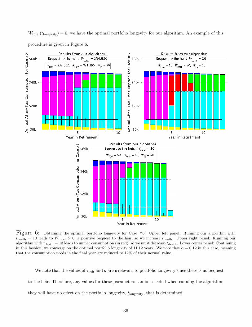
Wtotal(tlongevity) = 0, we have the optimal portfolio longevity for our algorithm. An example of this

procedure is given in Figure 6.

Figure 6: Obtaining the optimal portfolio longevity for Case #6. Upper left panel: Running our algorithm withtdeath = 10 leads to Wtotal > 0, a positive bequest to the heir, so we increase tdeath. Upper right panel: Running ouralgorithm with tdeath = 13 leads to unmet consumption (in red), so we must decrease tdeath. Lower center panel: Continuingin this fashion, we converge on the optimal portfolio longevity of 11.12 years. We note that α = 0.12 in this case, meaningthat the consumption needs in the final year are reduced to 12% of their normal value.

We note that the values of τheir and a are irrelevant to portfolio longevity since there is no bequest

to the heir. Therefore, any values for these parameters can be selected when running the algorithm;

they will have no effect on the portfolio longevity, tlongevity, that is determined.

36

6 Conversions of the TDA to a Roth or to a taxable

stock account

Our model for the algorithm presented in Subsection 4.3, by assumption, does not accommodate

conversions among the TDA, Roth account, and taxable stock account. Here, we consider the

opportunities that can be opened by removing that assumption. Since the Roth is tax-free, it is

never desirable to convert from the Roth account to the TDA or taxable stock account. As was

discussed in Section 1, after RMDs begin, the retiree is prohibited from draining a taxable stock

account to make TDA contributions. Also, if they have no earned income, they cannot drain the

taxable stock account to make Roth contributions.

This leaves possible conversions from the TDA account. Conversions of TDA RMDs must be to

taxable accounts, because IRS rules prohibit conversions of these RMDs to Roth accounts. Voluntary

TDA money, however, may be converted to Roth accounts (see Cook, Meyer, and Reichenstein

(2015)). In this section, we first consider conversions when TDA RMDs cause us to exceed our

consumption needs, C(t). Then we consider two ways where conversion of voluntary TDA money to

Roth accounts is useful. In all cases, our approaches in this section are only approximately optimal.

6.1 Converting excess TDA RMDs to taxable stock

TDA RMDs that cause the TDA +L(t) + U(t) to exceed C(t) must be used to buy taxable stock,

since it cannot be converted to a Roth account. To accommodate this conversion of RMDs to taxable

stock, in Stage 4 of Section 4.3, as we move chronologically through determining RMDs, if we hit a

year where the TDA RMDs go above C(t), we purchase taxable stock in that year with the after-tax

excess RMDs. This newly purchased taxable stock is combined with the after-tax dividends from

that year. We then freeze the strategy up to that year and rerun our algorithm on the later years.

37

This process is repeated for each subsequent year where the TDA RMDs cause consumption to

exceed C(t), until we reach tdeath.

6.2 Converting voluntary TDA money to a Roth account via over-

consumption

It may be the case that we stop using voluntary TDA money in some years because consumption

needs are satisfied, but in later years TDA money is consumed in a higher tax bracket. In this case

TDA to Roth conversions in these earlier years are advantageous, as they either replace the later

high tax bracket TDA spending with Roth spending or they provide more desirable Roth money to

the heir.

More specifically, we consider the marginal tax bracket of additional TDA spending in every

year, and then consider the earliest of the years that correspond to the lowest of these marginal tax

brackets. We then see if there is voluntary TDA spending in a later year at a tax bracket that is

higher than this lowest marginal tax bracket. If there is not, we remove considering conversions in

this year from all future iterations, and we iterate this process again. If there is, we consume TDA

money in this earliest, lowest tax bracket year until it fills its tax bracket, and then we convert this

additional TDA money to Roth money. This brings the TDA +L(t) consumption in this year to

the top of its marginal tax bracket, so, in subsequent iterations, the next higher tax bracket will be

associated with this year. We then freeze the strategy up to this (previously) lowest consumption

year, rerun our algorithm on all later years, and repeat this process until all years have been removed

from consideration.

After this process terminates, we consider the method in the next subsection, which details a

second way by which converting voluntary TDA money to Roth money can be useful.

38

6.3 Using taxable stock for consumption in place of the TDA,

which is then converted to a Roth

Cook, Meyer, and Reichenstein (2015) point out that voluntary TDA to Roth conversions can be

helpful to investors who are intending to use voluntary TDA money to address consumption needs

in a sufficiently early year. In these years, they point out that the investor is generally better off

using taxable stock to fill the consumption needs that were previously slated to be addressed by the

voluntary TDA money and then converting all the previously slated voluntary TDA money to Roth

money. This maneuver enables earlier spending of the taxable stock, which, by guiding principle

#2, is always advantageous. Since this is advantageous, there will always be enough Roth money

generated by the conversion to address any later gaps in addressing consumption that may occur

due to running out of taxable stock.

Our algorithm can be modified to incorporate the advantages of these conversions. We begin by

running our algorithm from Subsection 4.3, followed by the modifications in Subsections 7.1 and 7.2.

After running Subsection 7.2 we take note of the value of WTS(tdeath). Because we do not want to

diminish the beneficial effect to the heir of capital gains taxes being forgiven when the retiree dies,

we will not let the value of WTS(tdeath) be reduced by our process in this subsection.

Next we freeze the taxable stock and dividend consumption by temporarily treating it as part of

U(t), and then we shift the TDA spending in the transition tax bracket as far as possible to earlier

years, while still satisfying RMDs. This move has the potentially beneficial effect of increasing the

amount of early voluntary TDA money, enabling the conversion maneuver to be more effective.

Starting at t = 1, and then moving in chronological order, we apply the Cook, Meyer, and

Reichenstein conversion maneuver to any voluntary TDA spending. After each year where this ma-

neuver is applied, we freeze all spending in this year and the previous years, and reapply Subsection

4.3 and Subsection 7.1 and 7.2 to the remaining years with the newly altered worths of the Roth and

39

taxable stock accounts. At first, we run this allowing dividends, but no taxable stock, to be spent

in these remaining years, and we see if WTS(tdeath) has dipped below its original value. If it has, we

reduce the amount the maneuver was applied in this year until WTS(tdeath) again attains its original

value, and once this is the case, we are done. If it has not, we again reapply Subsection 4.3 and

Subsection 7.1 and 7.2 to the remaining years, but this time we allow both dividends and taxable

stock to be spent in these remaining years, and, once this is done, we proceed to the next year to

see if there is any voluntary taxable stock on which to perform the Cook, Meyer, and Reichenstein

conversion maneuver or, if the current year is tdeath, we are done.

7 Results

We discuss computed results from our algorithm for a variety of cases, where each case’s parameter

values can be found in Appendix 4. In all of our cases, we have employed the IRS tax brackets for

a single filer from 2016, which are also given in Appendix 4, although our program can also easily

accommodate changes to the thresholds, rates, and number of tax brackets, should Congress change

any of these. For the sake of simplicity, our computer program, as opposed to our algorithm, does

not consider situations that involve more than a single lot of taxable stock purchased prior to t = 1,

situations that involve RMDs that are so severe that Step 4.4 is triggered, or the use of conversions

as discussed in Section 6. The MATLAB R2017a computer program for our algorithm typically ran

in under 4 seconds on an iMac with a 4 GHz Intel Core i7 processor and 16 GB of 1867 MHz DDR3

memory.

7.1 Examples of our algorithm results

The three computed examples in Figure 7 demonstrate some of the wide range of behavior that our

algorithm captures. The two upper panels of Figure 7 are the final products of the algorithm for

40

Case #3 and Case #4, whose intermediate steps were presented in Subsection 4.3.

Figure 7: Algorithm results. Upper left panel: Case #3. Upper right panel: Case #4. Lower panel: Case #7.

For Case #3 in the upper left panel of Figure 7, we see that the solid horizontal line for Hheir is

at the top of the lowest tax bracket, which is the 10% bracket, because τheir = 13% here, which is less

than 15%, the rate for the second bracket. Ideally the TDA would only fill the area below Hheir and

nothing above, but RMDs require that more be filled, following guiding principle #5. After that,

it is hoped that the Roth and taxable stock accounts can fill the remainder. The optimal strategy

requires the taxable stock to be consumed as early as possible, following guiding principle #2. In

41

this case, we fill to the point where the taxable stock is exhausted, causing WTS(tdeath) = 0, then we

fill with the Roth. The Roth also becomes exhausted, causing WRoth(tdeath) = 0, so the remainder

of the consumption needs must be filled with “voluntary” TDA money. It is optimal for the Roth

to fill the two small parts of the consumption in years 8 and 9 that lie in the third tax bracket,

which is the 25% bracket, as TDA spending in this bracket would be highly taxed. However, by

guiding principle #1, the method in which the TDA and the Roth fill the 15% tax bracket, which

is the transition tax bracket in this case, does not matter, as long as the Roth is exhausted and all

consumption needs are satisfied.

For Case #4 in the upper right panel of Figure 7, we have known, fixed sources that create

L(t) and U(t) at the bottom and the top, respectively, of the consumption bars. In this case,

WTDA(tdeath), WRoth(tdeath), and WTS(tdeath) are all non-zero, so the TDA stays below Hheir and the

Roth stays above Hheir. Up through year 18, there is a stronger case to use taxable stock instead

of the Roth. That is, during this period, the forgiveness of capital gains for taxable stock when the

retiree dies is a weaker effect than the erosive effects of dividend taxes and the inability to shield the

heir’s subsequent gains from taxes. Starting in year 19, the forgiveness of capital gains for taxable

stock becomes the stronger factor, making using the Roth preferable to using taxable stock, so,

starting in year 19, only dividends are consumed from the taxable stock account, as required by

guiding principle #4. Similarly, up through year 8, there is a stronger case to use taxable stock

instead of the TDA in the 15% tax bracket, but, starting in year 9, this preference reverses.

From an economic point of view, C(t), L(t), and U(t) generally exhibit exponential growth or

decay. For example, C(t) may need to grow faster than inflation to accommodate increased medical

needs; L(t) may represent part-time work that decreases over time after retiring; or U(t) may be

a tax-free pension that grows with inflation and is therefore constant in real dollars. But this

restriction to exponential models is only for economic reasons. Our algorithm is capable of handling

42

any functions for C(t), L(t), and U(t) that we wish to model. Case #7 in the lower panel of Figure

7, for example, employs non-exponential functions for all three.

7.2 Comparison of our results with the naıve and informed strate-

gies

In the introduction, we discussed previous strategies non-academics and academics have employed

for drawing down funds in retirement, which Horan called naıve and informed strategies. In all of

these strategies, RMDs from the TDA are first satisfied. In naıve strategy #1, the retiree then

drains the taxable stock account, followed by the TDA, and finally the Roth. In naıve strategy #2,

the retiree then drains the taxable stock account, followed by the Roth, and finally the TDA. In an

informed strategy, the retiree drains the TDA up to the top of one of the tax brackets, and then

fills any excess consumption needs by first draining the taxable stock account, followed by the Roth,

and finally the TDA if it has not already been drained. The best informed strategy selects the tax

bracket with the best outcome.

Our algorithm’s approximations for the optimal solution are quite small compared to the approx-

imations in these other three strategies. Indeed, we have not found a case where either of the naıve

strategies or the best informed strategy are superior to the strategy generated by our algorithm.

This includes every case presented in this paper and the numerous other cases we have run but not

included here for the sake of space.

Case #8, for example, which is shown in Figure 8, was produced by considering an investor who

had a salary of $200,000 and followed two standard rules of thumb for retirement: 1) the investor

saved 10 times their salary before retiring, and 2) the investor planned on initially spending 70% of

their salary during retirement.9 Comparing the four strategies, we find that the size of the bequest,

9See, for example, https://www.fidelity.com/viewpoints/retirement/how-much-money-do-i-need-to -retire

43

Wtotal(tdeath), for our algorithm is highest, followed by the best informed strategy, naıve strategy

#1, and finally, naıve strategy #2.

Figure 8: Comparison of naıve strategy #1 (upper left panel), naıve strategy #2 (upper right panel), the best informedstrategy (lower left panel), and the strategy generated by our algorithm (lower right panel). We note that the best informedstrategy in this case fills the retiree’s consumption needs with TDA money up to the top of the third tax bracket, which isthe 25% bracket.

In Table 1, we find similar results for Case #6 and Case #9, where we compare optimal portfolio

longevity, instead of bequest size. Case #6 was previously presented in Figure 6. Case #9 somewhat

resembles the pictures for Case #8 in Figure 8, although it applies to a retiree with fewer needs and

fewer resources. For Case #6, the best informed strategy fills the retiree’s consumption needs with

44

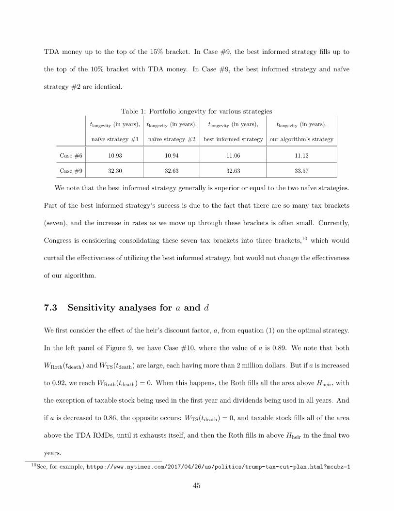
TDA money up to the top of the 15% bracket. In Case #9, the best informed strategy fills up to

the top of the 10% bracket with TDA money. In Case #9, the best informed strategy and naıve

strategy #2 are identical.

Table 1: Portfolio longevity for various strategies

tlongevity (in years), tlongevity (in years), tlongevity (in years), tlongevity (in years),

naıve strategy #1 naıve strategy #2 best informed strategy our algorithm’s strategy

Case #6 10.93 10.94 11.06 11.12

Case #9 32.30 32.63 32.63 33.57

We note that the best informed strategy generally is superior or equal to the two naıve strategies.

Part of the best informed strategy’s success is due to the fact that there are so many tax brackets

(seven), and the increase in rates as we move up through these brackets is often small. Currently,

Congress is considering consolidating these seven tax brackets into three brackets,10 which would

curtail the effectiveness of utilizing the best informed strategy, but would not change the effectiveness

of our algorithm.

7.3 Sensitivity analyses for a and d

We first consider the effect of the heir’s discount factor, a, from equation (1) on the optimal strategy.

In the left panel of Figure 9, we have Case #10, where the value of a is 0.89. We note that both

WRoth(tdeath) and WTS(tdeath) are large, each having more than 2 million dollars. But if a is increased

to 0.92, we reach WRoth(tdeath) = 0. When this happens, the Roth fills all the area above Hheir, with

the exception of taxable stock being used in the first year and dividends being used in all years. And

if a is decreased to 0.86, the opposite occurs: WTS(tdeath) = 0, and taxable stock fills all of the area

above the TDA RMDs, until it exhausts itself, and then the Roth fills in above Hheir in the final two

years.

10See, for example, https://www.nytimes.com/2017/04/26/us/politics/trump-tax-cut-plan.html?mcubz=1

45

Figure 9: Left panel: Case #10 for studying how sensitive the optimal strategy is to changes in the heir’s discountfactor, a. Right panel: Case #11 for studying the corrosive effect of dividends, d.

Given a choice between two stocks with an expected return of 5%, where one stock returns 4

of that 5% as dividends and the other gives no dividends, the heavy majority of retirees and their

advisors will pick the stock that returns dividends for reasons including that dividend paying firms

are often considered to be more stable than non-dividend paying firms. From a taxation point of

view, however, this is a considerable mistake. It is well known for long term stock investing that

the loss of deferring capital gains taxes due to an intermediate sale and repurchase of a stock can

have a considerable negative impact on the total gains after the final sale of the stock. Assuming

τgains = τdiv, dividends are like a forced intermediate sale, except that dividends are worse for two

reasons: 1) The sale of normal stock is at the cost basis, ω, of the lot being sold, but dividends are

like a sale on just the gains. That is, it is a sale on a part of the lot where ω = 0, the worst case. 2)

The fact that dividends then lower ω for the rest of the lot will partially compensate for this if the

stock is later sold by the retiree. But once the retiree stops using taxable stock for consumption,

this lot will not be sold by the retiree. It will go to the heir, where all gains are forgiven and the

fact that ω was lowered for the retiree becomes irrelevant.

46

Consider Case #11 shown in the right panel of Figure 9, where the investor starts with a million

dollars in taxable stock, a = 1, and the dividend rate is d = 4%. All the magenta in the panel

represents dividends, which are optimally used for consumption by general principle #4. If we now

change the dividend rate to d = 0, the magenta part will be replaced by the Roth in green, and the

value of Wtotal(tdeath) will increase from $3,239,007 to $3,563,895. That is, in this case, if the retiree

chooses the stock without dividends for their taxable account, their heir will receive $324,888 more

dollars.

8 Conclusions

Previous strategies for how a United States retiree should allocate their withdrawals in a tax efficient

manner among TDAs, Roth accounts, and taxable stock accounts have not depended on the amounts

in these three accounts, nor on the parameters governing them. In this paper, we have presented an

algorithm that uses these amounts and parameters to develop a strategy that adapts to the retiree’s

specific circumstances. The development of our algorithm reveals insights into the complex structure

governing the trade-offs in using these three accounts to satisfy retiree consumption needs. This is

particularly challenging with the taxable account, since its tax structure differs significantly from

the tax structure of the TDA and the Roth account.

Our algorithm starts by using tax law to create five guiding principles that govern prioritizing

consumption from the three accounts: 1) We prove that if the retiree consumes a given amount of

Roth money and given amounts of TDA money at various marginal tax rates, the order/allocation

in which these are consumed is irrelevant; 2) In contrast, taxable stock and dividends are better

spent earlier rather than spent later; 3) When consuming taxable stock, the lot with the highest

cost basis should always be tapped; 4) Dividends should always be consumed before Roth money;

and 5) Required Minimum Distributions (RMDs) should always be taken out of any TDA. These

47

five guiding principles help us develop desirability factors for the three accounts. These desirability

factors help us determine the most favorable annual allocations among the accounts that satisfy

the consumption needs of the retiree. Our algorithm incorporates a number of standard features

studied in the research literature, such as working with RMDs from the TDA account and optimizing

portfolio longevity, as well as a number of less standard features, such as incorporating the effect

of dividends, optimizing a bequest to an heir, allowing for two types of additional fixed sources

of money for the retiree, accommodating different taxable lots in the taxable stock account, and

working with conversions from the TDA to both the Roth account and the taxable stock account.

We explain why the taxation structure for dividends can produce large, negative effects in a

retiree’s taxable stock portfolio. The magnitude of these effects, which can be quantified with

our algorithm, suggests that, contrary to conventional wisdom, many retirees would be better off

avoiding, instead of prizing, dividend paying stocks in their taxable accounts. Our algorithm appears

to be a significant improvement over the previous naıve and informed strategies, which are the most

common strategies in the academic and non-academic literature for withdrawing money in retirement.

We were unable to find a case where these previous strategies were superior to the strategy produced

by our algorithm, nor would we expect to, except in unusual circumstances, and, even then, only by

minute amounts.

References

[1] Al Zaman, Ashraf. 2008. “Reconsidering IRA and Roth IRA: Keeping Bequests and Other

Options in Mind.” Journal of Wealth Management, Fall: 82–92.

[2] Brown, David C., Scott Cederburg, and Michael S. O’Doherty. 2016. “Tax Uncertainty and

Retirement Savings Diversification” Journal of Financial Economics, forthcoming.

48

[3] Cook, Kristen A., William Meyer, and William Reichenstein. 2015. “Tax-Efficient Withdrawal

Strategies” Financial Analysts Journal, vol. 71, no. 2: 16–29.

[4] Coopersmith, Lewis W. and Sumutka, Alan R. 2011. “Tax-Efficient Retirement Withdrawal

Planning Using a Linear Programming Model” Journal of Financial Planning, September: 50–

59.

[5] Dammon, Robert M., Spatt, Chester S., and Zhang, Harold H. 2004. “Optimal Asset Location

and Allocation with Taxable and Tax-Deferred Investing” The Journal of Finance, vol. 59,

no. 3, June: 999–1037.

[6] DiLellio, James A. and Ostrov, Daniel N. 2017. “Optimal Strategies for Traditional versus Roth

IRA/401(k) Consumption During Retirement”, Decision Sciences, vol. 48, pp. 356-384.

[7] Fidelity. 2014. “Four Tax-Efficient Strategies in Retirement.” www.fidelity.com/viewpoints/

retirement/tax-savvy-withdrawals.

[8] Fidelity. 2015. “Detailed Methodology, Retirement Income Planner” http://personal.

fidelity.com/planning/retirement/pdf/rip_methodology.pdf, April 2015.

[9] Huang, Chye-Ching and Brandon DeBot. April 2005. “Ten Facts You Should Know About the

Federal Estate Tax”. Center on Budget and Policy Priorities.

[10] Horan, Stephen M. 2006a. “Withdrawal Location with Progressive Tax Rates.” Financial An-

alysts Journal, vol. 62, no. 6: 77–87.

[11] Horan, Stephen M. 2006b. “Optimal Withdrawal Strategies for Retirees with Multiple Savings

Accounts.” Journal of Financial Planning, vol. 19, no. 11, November: 62–75.

[12] Jaconetti, Colleen M., and Maria A. Bruno. 2008. “Spending from a Portfolio: Implications of

Withdrawal Order for Taxable Investors.” Vanguard Research, 1–13.

[13] Lange, James. 2009. Retire Secure! Wiley, ISBN: 0470405317.

49

[14] Larimore, Taylor, Lindauer, M., Ferri, R.A., and Dogu, L.F. 2011. The Bogleheads’ Guide To

Retirement Planning. Wiley, ISBN: 0470919019.

[15] Nocedal, Jorge, and Wright, Stephen. Numerical Optimization, Springer, 2006.

[16] Ostrov, Daniel N. and Thomas G. Wong. 2011. “Optimal Asset Allocation for Passive Investing

with Capital Loss Harvesting”, Applied Mathematical Finance, vol. 18, no. 4, pp. 291–329.

[17] Piper, Mike. 2013. Can I Retire? Simple Subjects, LLC, ISBN: 0981454259.

[18] Reichenstein, William, Stephen M. Horan, and William W. Jennings. 2012. “Two Key Concepts

for Wealth Management and Beyond.” Financial Analysts Journal, vol. 68, no. 1: 14–22.

[19] Rodgers, Rick. 2009. The New Three-Legged Stool. Wiley, ISBN: 1592803636.

[20] Rosato, Donna. 2015. “Can I Put My Required Minimum Distribu-

tion into a Roth IRA?” Money: http://time.com/money/3835309/

retirement-required-minimum-distribution-roth/, April 28, 2015.

[21] Shoven, John B. and Sialm, Clemens 2003. “Asset location in tax-deferred and conventional

savings accounts.” Journal of Public Economics, vol. 88: pp. 23?38.

[22] Solin Daniel R. 2010. The Smartest Retirement Book You’ll Ever Read. Perigee Trade, ISBN:

0399536345.

[23] Spitzer, John J. and Singh, Sandeep 2006. “Extending Retirement Payouts by Optimizing the

Sequence of Withdrawals,” Journal of Financial Planning, vol. 19, no. 4, April: 52–61.

[24] Sumutka, Alan R., Andrew M. Sumutka, and Lewis W. Coopersmith. 2012. “Tax-Efficient

Retirement Withdrawal Planning Using a Comprehensive Tax Model.” Journal of Financial

Planning, April: 41–52.

50

[25] Vanguard. 2013. “How to Turn Retirement Savings into Retirement Income.”

https://retirementplans.vanguard.com/ekit/pmed/retirement_income_center/pdf/

RILongBroc.PDF

Appendix 1: Proof that the withdrawal strategy between

a TDA taxed at a constant tax rate versus a Roth account

does not matter.

Define T (t) and R(t) to be the worths of the TDA and Roth account respectively, which we assume

grow at the same rate, µ(t). Define CT (t) and CR(t) be the continuous time after-tax consumption

rates chosen for the TDA and Roth account respectively. Finally, we assume that the TDA is taxed

at a constant rate, τ , when money is taken out from it to satisfy consumption. Given this, the TDA

is governed by the ordinary differential equation (ODE)

dT

dt= µ(t)T (t)− CT (t)

1− τ,

and the Roth account is governed by the ODE

dR

dt= µ(t)R(t)− CR(t).

Let C(t) be the total, fixed, after-tax consumption rate for the retiree’s needs, so CT (t) and CR(t)

need to be chosen so that CT (t) + CR(t) = C(t). We define α(t) to be the fraction of the total

consumption met by the TDA, i.e., CT = α(t)C(t), and therefore 1−α(t) is the fraction of the total

consumption met by the Roth account, i.e., CR(t) = (1 − α(t))C(t). When T > 0 and R > 0, the

51

retiree can choose α to take any value between 0 and 1. If T > 0 and R = 0, then α must be 1, and

if T = 0 and R > 0, then α must be 0. Should the portfolio reach the state T = R = 0, we are at

the time tlongevity, as the retiree is out of money.

The key question is “Does the retiree’s choice for consumption allocation between the TDA at a

constant tax rate and the Roth account matter?” or, equivalently in our notation, “Does the retiree’s

choice for α(t) matter?” Conventional wisdom generally suggests that it does, as indicated by the

many references in the introduction that advocate using one of the naıve strategies. Academic

research, on the other hand, suggests that it doesn’t. For example, Cook et al. (2015) give two

convincing, illustrative examples in discrete time with µ and C constant, where portfolios with x

Roth dollars last exactly as long as portfolios with x1−τ TDA dollars. DiLellio and Ostrov (2017)

show analytically in continuous time with any constant µ and C and any initial positions, T (0) and

R(0), that a portfolio lasts just as long when the TDA is drained (α = 1) and then the Roth is

drained (α = 0) as when the Roth is drained and then the TDA is drained.

We extend these results with a surprisingly simple argument to show that every strategy α(t)

leads to the same portfolio longevity, even when µ and C are functions of time. The argument is to

simply multiply the ODE for the TDA

dT

dt= µ(t)T (t)− α(t)C(t)

1− τ,

by (1− τ) and add it to the ODE for the Roth account,

dR

dt= µ(t)R(t)− (1− α(t))C(t), (2)

to obtain the ODE

dW

dt= µ(t)W (t)− C(t), (3)

52

where W (t) = R(t) + (1 − τ)T (t). The fact that α(t) does not appear in equation (3) establishes

why the strategy, α(t), chosen by the retiree does not matter. The definition of W (t) fits with the

statement in Cook et al. (2015) that x Roth dollars are equivalent to x1−τ TDA dollars, since W = x

in either case.

Should we want to determine W (t), we simply solve the linear ODE, equation (3), by multiplying

equation (3) by an integrating factor

e−∫ t0 µ(s)ds

(dW

dt− µ(t)W (t)

)= −e−

∫ t0 µ(s)dsC(t),

applying the product rule

d

dt

(e−∫ t0 µ(s)dsW (t)

)= −e−

∫ t0 µ(s)dsC(t),

and then integrating from time 0 to an arbitrary time t to obtain

W (t)e−∫ t0 µ(τ)dτ −W (0) = −

∫ t

0e−∫ s0 µ(τ)dτC(s)ds (4)

or, equivalently,

W (t) = W (0)e∫ t0 µ(τ)dτ −

∫ t

0e∫ ts µ(τ)dτC(s)ds.

Assuming C(t) is sufficiently big, there will be a time, tlongevity, where the portfolio becomes

exhausted. When this happens, from equation (4), we have that

R(0) + (1− τ)T (0) =

∫ tlongevity

0e−∫ s0 µ(τ)dτC(s)ds, (5)

since W (0) = R(0)+(1−τ)T (0) and W (tlongevity) = 0. Again, we note from equation (5) that tlongevity

53

is unaffected by the retiree’s choice of α(t). If, for example, µ is constant and the consumption grows

or decays exponentially, so C(t) = C(0)ekt, we can solve equation (5) to obtain

tlongevity =1

k − µln

(1 +

k − µC(0)

(R(0) + (1− τ)T (0))

).

We note that tlongevity only exists when k−µC(0)(R(0)+(1−τ)T (0)) > −1, since the portfolio never runs

out of money if k−µC(0)(R(0) + (1− τ)T (0)) ≤ −1. For the subcase where µ and C are both constant,

we simply set k = 0, yielding

tlongevity = − 1

µln(

1− µ

C(R(0) + (1− τ)T (0))

),

which agrees with the result given in DiLellio and Ostrov (2017).

Finally, we note that this continuous time proof is easily converted into a discrete time proof:

again, we simply show that changes to W do not depend on the retiree’s choice of α.

Appendix 2: Derivation of amin, the lower bound on the

heir’s discount factor

Recall that a is defined as the ratio of the worth to an heir of a dollar inherited in a taxable account

to a dollar inherited in a Roth account. The upper bound on a is a = 1, which corresponds to the

heir liquidating their Roth immediately upon inheriting it, since, at that time, neither the Roth nor

the taxable stock account are subject to tax, due to the forgiveness of all taxable gains when the

retiree dies. Of course, this is the worst case scenario for the heir. In this appendix, we derive a

formula for amin, the lower bound on a, which corresponds to the best case scenario, where the heir

liquidates their Roth account as slowly as possible by only taking RMDs.

54

To determine amin, our approach will be to exhaust the Roth, which is initially worth, say, M0

dollars, as slowly as possible through RMDs and then find the initial worth of a comparable taxable

stock account that, after providing the heir with the same after-tax payouts as the Roth RMDs,

exhausts itself at the same time as the Roth. Because this Roth account and this taxable stock

account are of equal worth to the heir, the initial worth of the taxable account must be M0amin

, which

determines amin.

According to current IRS rules, if at t = tdeath, the heir has a life expectancy of Their more years

to live, then the heir’s RMDs are 1Their

of their Roth money (and of their TDA money) in the first

year of their inheritance, followed by 1Their−1 of their Roth (and TDA) money in the second year,

then 1Their−2 in their third year, etc., so their Roth (and TDA) portfolios are completely liquidated

in the Their− 1 year of their inheritance.11 Since our analysis will be in continuous time, we will use

continuous time analogues of these RMD rules, and we will use µc = ln(1 + µ) and dc = ln(1 + d),

which are the continuous time versions of µ and d. We will also assume that dividends are always

produced at a rate that is smaller than the Roth RMDs (i.e., d ≤ 1Their

). Finally, we redefine the

time t = 0 to now correspond to the time when the heir begins their inheritance.

We begin with the Roth account. Letting MR(t) represent the amount of money in the Roth

account at time t, the continuous form of the IRS’s RMD rules forces us to liquidate the account at

a rate of MR(t)Their−t dollars per year. Therefore, MR is governed by the differential equation

dMR

dt= µcMR −

MR

Their − t,

11Here we are assuming the heir is not a spouse. If the heir is a spouse, the spouse has no Roth RMDs, and the spousehas a variety of options for any inherited TDA (i.e., leave the TDA in the name of the deceased, roll it into an inheritedIRA, or roll it into a spousal IRA). Each of these choices potentially affects the value of amin.

55

subject to the initial condition MR(0) = M0. Separating variables

dMR

MR=

(µc −

1

Their − t

)dt

and integrating using the initial condition yields

MR(t) =M0

Their

eµct(Their − t).

That is, we liquidate the Roth account at a rate of MR(t)Their−t = M0

Theireµct (tax-free) dollars per year.

Now we look at the taxable account. Dividends are created at a rate of dcMT (t), where MT (t)

represents the amount of money in the taxable account at time t. Since we have to pay taxes

on the dividends at a rate of τdiv, the dividends generate after-tax cash at a continuous rate of

(1− τdiv)dcMT .

In addition to using these dividends, we need to sell stock at an after-tax rate of M0Their

eµct− (1−

τdiv)dcMT to keep the same after-tax cash flow as the Roth account. Given that the capital gains tax

rate on any stock sold will be τgains(1− e−(µc−dc)t), this means we need to sell stock at a before-tax

rate ofM0Their

eµct − (1− τdiv)dcMT

1− τgains(1− e−(µc−dc)t).

Given this, MT (t) is governed by the differential equation

dMT

dt= (µc − dc)MT −

M0Their

eµct − (1− τdiv)dcMT

1− τgains(1− e−(µc−dc)t).

Since this equation is linear, it can be put in the form

dMT

dt+ f(t)MT = g(t),

56

where

f(t) = −[(µc − dc) +

(1− τdiv)dc

(1− τgains) + τgainse−(µc−dc)t

]and

g(t) =− M0Their

eµct

(1− τgains) + τgainse−(µc−dc)t.

Multiplying the equation by the integrating factor

I(t) = e∫f(t)dt = e−(µc−dc)t

(e(µc−dc)t +

τgains1− τgains

)− (1−τdiv)dc(1−τgains)(µc−dc)

and applying the product rule transforms the linear equation into the form

d(MT (t)I(t))

dt= I(t)g(t).

Recall that we start with MT (0) = M0amin

dollars, which are to be completely drained by the Roth-size

cash flows by time Their, so MT (Their) = 0. Therefore, if we integrate between t = 0 and t = Their,

we have that

−I(0)M0

amin=

∫ Their

0I(t)g(t)dt.

Finally, using the full expressions for I and g and isolating amin yields

amin =

1

Their

∫ Their

0eµct

((1− τgains)e(µc−dc)t + τgains

)−(1+ (1−τdiv)dc(1−τgains)(µc−dc)

)dt

−1

. (6)

If we assume that dividends are negligible, then we set dc = 0 in (6), which reduces to simply

amin =µcTheir(1− τgains)

ln((1− τgains)eµcTheir + τgains

) . (7)

Note that as Their → 0 in (7), by L’Hopital’s Rule we have that amin → 1 as expected. Also, as

57

Their → ∞, we have that amin → (1 − τgains), which is also expected, since, in this limit, taxes on

capital gains still occur, but the disadvantage of having to pay them earlier vanishes. Similarly, for

(6), as Their → 0, amin → 1, and, if τgains = τdiv (as is the case for most long-term investors), then as

Their → ∞, amin → (1 − τgains)µc

µc−dc . Of course, letting Their → ∞ corresponds to a lower value for

amin, so if we use typical values like τgains = 0.15, µc = 0.06, and dc = 0.02, we produce the low-ball

estimate amin = (1− 0.15)0.06

0.06−0.02 = 0.78; hence our statement in Section 1 that amin ≥ 0.75 under

typical circumstances.

Appendix 3: Updating the worth of the TDA, Roth, and

taxable stock accounts during a given year

Update process for the Roth account

Notation:

sRoth is the worth of the stock in the Roth account.

MRoth are the after-tax consumption needs to be satisfied by the Roth account.

1. At the beginning of year t, use the Roth to satisfy the MRoth (after-tax) dollars

of consumption needs.

sRoth = sRoth −MRoth

2. Account for the gains over the year, noting that all dividends are reinvested, so

they have no effect.

58

sRoth = sRoth(1 + µ)

Update process for the TDA

Notation:

sTDA is the pre-tax worth of the TDA stock.

τmarg,k is the value of τmarg in the kth tax bracket, where k = 1 is the lowest tax bracket and kmax

is highest tax bracket in which TDA stock will be consumed.

MTDA,k are the after-tax consumption needs to be satisfied by TDA money in the kth tax bracket.

1. At the beginning of year t, use the TDA to satisfy thekmax∑k=1

MTDA,k (after-tax)

dollars of consumption needs.

For k = 1 to kmax

sTDA = sTDA −MTDA,k1−τmarg,k

2. Account for the gains over the year, noting that all dividends are reinvested, so

they have no effect.

sTDA = sTDA(1 + µ)

Update process for the taxable stock account

Notation:

59

sTS,j is the pre-tax worth of the stock in lots j = 1, 2, ..., jmax.

ωj is the fraction of the stock in lot j that is in the cost basis, where j = 1, 2, ..., jmax. That is, the

current cost basis in lot j is ωjsTS,j .

MTS are the after-tax consumption needs to be satisfied by dividends and capital gains.

1. At the end of year t−1, take dividends out of all the lots of stock, which decreases

their worth, but increases their cost basis fraction, ω. Use these dividends, after paying

taxes on them, to buy a new lot of stock.

For j = 1 to jmax

sTS,j = sTS,j(1− d)

ωj =ωj1−d

jmax = jmax + 1 (create the new lot)

sTS,jmax = (1− τdiv)d

(jmax−1∑j=1

sTS,j

)

ωjmax = 1

2. At the beginning of year t, use the taxable stock account to satisfy the MTS

(after-tax) dollars of consumption needs.

For j = jmax to 1 (note decrement, not increment)

if MTS ≥ sTS,j [1− τgains(1− ωj)] (There are more consumption needs than lot j can satisfy.)

MTS = MTS − sTS,j [1− τgains(1− ωj)] (Exhaust all lot j stock for consumption.)

sTS,j = 0

else

sTS,j = sTS,j −MTS

1−τgains(1−ωj)(Sell just enough stock to satisfy remaining consumption needs)

60

MTS = 0

jmax = j (since there are only j lots left)

break

3. Account for the gains over the year, just prior to dividend distributions.

For j = 1 to jmax

sTS,j = sTS,j(1 + µ)

ωj =ωj1+µ

Appendix 4: Parameter values for computations

The following table gives the parameter values for all the cases presented in this paper:

61

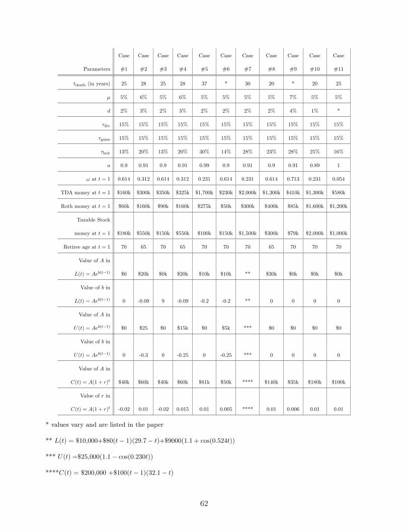
Case Case Case Case Case Case Case Case Case Case Case

Parameters #1 #2 #3 #4 #5 #6 #7 #8 #9 #10 #11

tdeath (in years) 25 28 25 28 37 * 30 20 * 20 25

µ 5% 6% 5% 6% 5% 5% 5% 5% 7% 5% 5%

d 2% 3% 2% 3% 2% 2% 2% 2% 4% 1% *

τdiv 15% 15% 15% 15% 15% 15% 15% 15% 15% 15% 15%

τgains 15% 15% 15% 15% 15% 15% 15% 15% 15% 15% 15%

τheir 13% 20% 13% 20% 30% 14% 28% 23% 28% 25% 16%

a 0.9 0.91 0.9 0.91 0.99 0.9 0.91 0.9 0.91 0.89 1

ω at t = 1 0.614 0.312 0.614 0.312 0.231 0.614 0.231 0.614 0.713 0.231 0.054

TDA money at t = 1 $160k $300k $350k $325k $1,700k $230k $2,000k $1,300k $410k $1,300k $580k

Roth money at t = 1 $60k $160k $90k $160k $275k $50k $300k $400k $85k $1,600k $1,200k

Taxable Stock

money at t = 1 $180k $550k $150k $550k $100k $150k $1,500k $300k $79k $2,000k $1,000k

Retiree age at t = 1 70 65 70 65 70 70 70 65 70 70 70

Value of A in

L(t) = Aeb(t−1) $0 $20k $0k $20k $10k $10k ** $30k $0k $0k $0k

Value of b in

L(t) = Aeb(t−1) 0 -0.09 9 -0.09 -0.2 -0.2 ** 0 0 0 0

Value of A in

U(t) = Aeb(t−1) $0 $25 $0 $15k $0 $5k *** $0 $0 $0 $0

Value of b in

U(t) = Aeb(t−1) 0 -0.3 0 -0.25 0 -0.25 *** 0 0 0 0

Value of A in

C(t) = A(1 + r)t $40k $60k $40k $60k $81k $50k **** $140k $35k $180k $100k

Value of r in

C(t) = A(1 + r)t -0.02 0.01 -0.02 0.015 0.01 0.005 **** 0.01 0.006 0.01 0.01

* values vary and are listed in the paper

** L(t) = $10,000+$80(t− 1)(29.7− t)+$9000(1.1 + cos(0.524t))

*** U(t) =$25,000(1.1− cos(0.230t))

****C(t) = $200,000 +$100(t− 1)(32.1− t)

62

The following table gives the incomes at which each IRS tax bracket begins for a single filer in 2016 (see

https://www.irs.com/articles/2016-federal-tax-rates-personal-exemptions-and

-standard-deductions):

Bracket tax rate 10% 15% 25% 28% 33% 35% 39.6%

Bottom of the bracket in pre-tax dollars 0 $9,275 $37,650 $91,150 $190,150 $413,350 $415,050

Bottom of the bracket in after-tax dollars 0 $8,347.50 $32,466.25 $72,591.25 $143,871.25 $293,415.25 $294,520.25

We note that because our bar graphs are in after-tax dollars, the after-tax values in the final row of our table

correspond to the heights of the dashed and solid horizontal lines in the bar graphs.

63