Journal of Mathematical Psychology 55 (2011) 106–117

Contents lists available at ScienceDirect

Journal of Mathematical Psychology

journal homepage: www.elsevier.com/locate/jmp

Constructing informative model priors using hierarchical methodsWolf VanpaemelDepartment of Psychology, University of Leuven, Tiensestraat 102, B-3000 Leuven, Belgium

a r t i c l e i n f o

Article history:Received 6 February 2010Received in revised form8 July 2010Available online 8 October 2010

Keywords:BayesHierarchicalEstimationPriorsInformativeSubjectiveAbstractionCategory learning

a b s t r a c t

Despite their negative reputation, informative priors are very useful in inference. Priors that express psy-chologically meaningful intuitions damp out random fluctuations in the data due to sampling variability,without sacrificing flexibility. This article focuses on how an intuitively satisfying informative prior dis-tribution can be constructed. In particular, it demonstrates how the hierarchical introduction of a param-eterized generative account of the set of models under consideration naturally imposes a non-uniformprior distribution over the models, encoding existing intuitions about the models. The hierarchical ap-proach for constructing informative model priors is made concrete using a worked example, the VaryingAbstraction Model (VAM), a family of categorization models including and expanding the exemplar andprototype models. It is shown how psychological intuitions about the relative plausibilities of the modelsin the VAM can be formally captured in an informative prior distribution over these models, by specify-ing a theoretically informed process for generating the models in the VAM. The smoothing effect of theinformative prior in estimation is demonstrated by considering ten previously published data sets fromthe category learning literature.

© 2010 Elsevier Inc. All rights reserved.

1. Introduction

Rouder, Lu, Speckman, Sun, and Jiang (2005, p. 198) tell thefollowing (true) anecdote from a baseball game:

In the late summer of 2000, the struggling Kansas City Royalswere hosting the Boston Red Sox. Pitching for Bostonwas PedroMartínez, who was having a truly phenomenal year. Many inthe crowd came to see Martínez and his dominant pitching.Contrary to expectation, in the first inning, Kansas City scoredfive runs, and Boston none. At the end of the first inning, oneof our colleagues, who is a loyal Royals fan and an APA editor,predicted a final score of 45–0.

There is a lot of logic to the prediction of 45–0, because it followsfrommultiplying the score after one inning by the total number ofinnings in a baseball game. However, it turned out to be far awayfrom the truth. Rouder et al. (2005, p. 198) recount:

After the first inning, Martínez pitched well, allowing only oneadditional run. Kansas City lost the game by a score of 7–6;Martínez was the winning pitcher.

It seems that it should be possible to come up with a betterprediction than the logical one that turnedout to be so dramaticallywrong. Fortunately, there is an easy remedy: adding knowledge

E-mail address:wolf.vanpaemel@psy.kuleuven.be.URL: http://ppw.kuleuven.be/concat.

0022-2496/$ – see front matter© 2010 Elsevier Inc. All rights reserved.doi:10.1016/j.jmp.2010.08.005

about baseball to the prediction. Even the slightest knowledge ofbaseball, such as knowing that there has never been a professionalbaseball game with a score as extreme as 45–0, would havedramatically improved the prediction of the final score. Moredetailed knowledge of the game, such as a (rough) distributionof final baseball scores, would have resulted in an even betterprediction. A baseball expert knowing that Boston was superior toKansas City and had the best pitcher might even have come closeto nailing the final score. In sum, the prediction could have beenvastly improved by combining the observation of the score afterone inning with some knowledge about the game.

1.1. The ugly duckling called prior

This example highlights the major theme of this article: usingknowledge about what is plausible can smooth inference, in thesense that it can prevent one from reaching extreme or unreason-able conclusions. Including such knowledge is greatly facilitated bythe adoption of the Bayesian framework, which provides a coher-ent andprincipledway to combine information fromobserved datawith information from additional knowledge that does not dependon the data. The Bayesian framework achieves this by augment-ing the likelihood function with a distribution for parameters andmodels, the prior, which provides an opportunity to incorporateadditional knowledge and intuitions. A prior could, for example,encode that final scores in professional baseball games rarely ex-ceed 10.

The ability to take relevant prior knowledge into account ininference is one of the major distinctions between the Bayesian

W. Vanpaemel / Journal of Mathematical Psychology 55 (2011) 106–117 107

framework and the standard framework (Lindley & Phillips, 1976).Most standard methods tend to ignore the prior knowledge that isavailable in a problem. For example, maximum likelihood estima-tion implicitly and by default assumes a uniform prior (see foot-notes 4 and 8), which does not encode any additional informationabout the plausibility of parameter values ormodels. Priors that, incontrast, are intended to express this sort of knowledge are calledinformative.

Informative priors are an often maligned aspect of Bayesianinference. As a result, most current psychological modeling ex-plicitly or implicitly relies on uniform priors, thereby closing itseyes to additional knowledge, theory, assumptions or intuitionsthat might exist. This unfortunate state of affairs has at least twogrounds, both conceptual and practical (Goldstein, 2006). A first,conceptual objection to including prior knowledge in the form ofan informative prior is that this practice is considered to makeinference inherently and irremediably subjective. It is often arguedthat informative priors corrupt scientific thinking,which seizes thehigh ground of objectivity, into mere wishful thinking (e.g., Efron,1986). From this perspective, informative priors are inappropriatefor reaching scientific conclusions and have no place in scientificanalyses (see, e.g., Lindley, 2004; Wagenmakers, Lee, Lodewyckx,& Iverson, 2008, for discussions).

A second, practical reason for the current underuse of informa-tive priors in psychological modeling relates to a lack of methodsfor formalizing prior knowledge or intuitions. Even when theoristshave clear prior intuitions about the parameters ormodels they aredealing with, and even if they are convinced that the inference willbenefit from including these intuitions, they are still confrontedwith the challenging problem of quantifying these intuitions in or-der to make quantitative inferences.

Contrary to the widespread view that the influence of the prioron inference should be minimized, I regard informative priors tobe highly useful in inference, chiefly for their capacity to pull thedata away from inappropriate and implausible inferences, withoutlosing useful flexibility. Adding prior knowledge or intuitions, inthe form of a non-uniform, informative prior should be pursuedmuch more often than is the case now. The present articlemainly addresses the practical objection to informative priors,by illustrating a generally applicable mechanism for formallycapturing existing intuitions about models in an informative priordistribution over the models.

1.2. Outline

This article provides a detailed demonstration of how a theo-retically motivated, informative prior distribution over models ina model family can be obtained by hierarchically extending themodel family with a parameterized account of how themodels aregenerated. The demonstration of how hierarchical methods can beused to construct an informative prior overmodels in amodel fam-ily focuses on the Varying Abstraction Model (VAM: Vanpaemel &Storms, 2008) as a case study. The VAM is a model family that en-compasses a range of categorizationmodels, including the familiarexemplar and prototype models, as well as various other modelsthat can be considered intermediate between these two extremes.

After providing an introduction to the VAM family, it is shownhow existing intuitions about the relative plausibilities of themodels in the VAM can be formally translated into an informativeprior distribution over these models. A key role is played bya process that, informed by psychological intuitions about themodels in the VAM, details how these models are generated. Usingten previously published data sets from the category learningliterature, it is illustrated how, just like in the baseball example,adding prior knowledge in the mix can smooth inference. Finally,the discussion touches upon the conceptual reason behind the

underuse of informative priors and reflects on the relation betweeninformative priors and subjectivity.

Before we get started, I provide a second example of how priorknowledge can smooth inference, focusing on a simple coin tossingproblem. Apart from an additional motivation of why includingprior intuitions in inference is desirable, this example also providesthe necessary Bayesian background for the more involved VAMexample. The coin tossing example thus serves as a mini-tutorialfor readers without a working knowledge of Bayesian methods.

2. Using an informative prior to smooth estimation

The Bayesian approach to estimation is most easily introducedusing a simple coin tossing example (see also Griffiths, Kemp, &Tenenbaum, 2008; Lee & Wagenmakers, 2005; Lindley & Phillips,1976). The probability of a sequence of n coin tosses containing hheads and t = n−h tails being generated by a coinwhich producesheads with probability π is

h ∼ Binomial(n, π), (1)

with

π ∈ [0, 1]. (2)

Based on an observed sequence of heads and tails, we would liketo estimate the value of π .

2.1. The maximum a posteriori (MAP) estimate

Treating π as a random variable, the initial (i.e., before the dataare collected) assumptions or knowledge about which values of πare likely and unlikely is represented in a distribution, p(π). Toreflect that this distribution is independent of observed data andthus can be expressed before data are observed, it is referred to asthe prior. After observing data d, such as the number of heads in acoin tossing sequence, the prior distribution p(π) is updated to theposterior distribution p(π | d), representing the knowledge aboutπ based upon the combination of the initial assumptions and theobserved data. Updating takes place according to Bayes’ rule:

p(π | d) =P(d | π)p(π)

P(d), (3)

where P(d | π) is the likelihood, indicating the probability of thedata given π , and P(d) a normalizing constant given by

P(d) =

∫Ωπ

P(d | π)p(π)dπ, (4)

with Ωπ the range of π .One commonly used method to obtain a point estimate1 from

the posterior distribution is maximum a posteriori (MAP) estima-tion: choosing the value of π that maximizes the posterior proba-bility,

πMAP = argmax p(π | d) = argmaxP(d | π)p(π)

P(d). (5)

Note that, since P(d) does not depend upon π , this term doesnot affect πMAP and can be omitted in the computation of πMAP;i.e., πMAP = argmax P(d | π)p(π). Accordingly, computing πMAPdoes not require the integral of (4) to be evaluated, but only re-quires an optimization algorithm.

1 Because reducing the full distribution p(π | d) to a single number like πMAPdiscards useful information, such as the uncertainty about the estimate, it is oftenpreferable to maintain the full posterior distribution.

108 W. Vanpaemel / Journal of Mathematical Psychology 55 (2011) 106–117

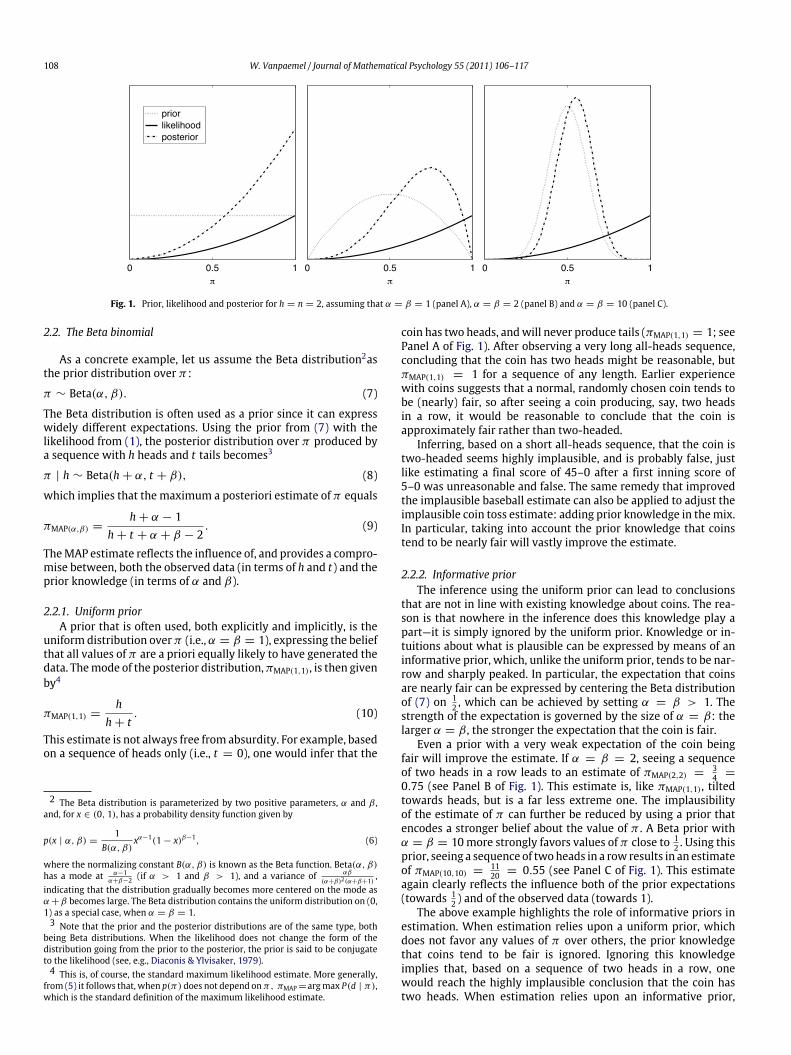
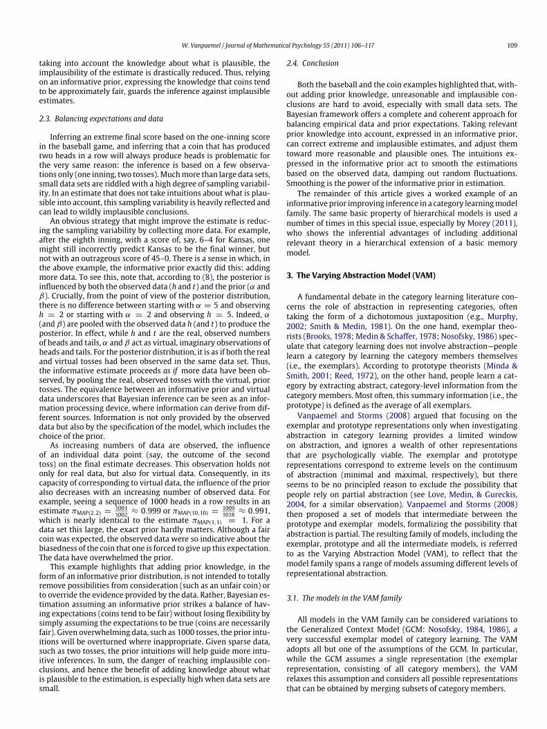
Fig. 1. Prior, likelihood and posterior for h = n = 2, assuming that α = β = 1 (panel A), α = β = 2 (panel B) and α = β = 10 (panel C).

2.2. The Beta binomial

As a concrete example, let us assume the Beta distribution2asthe prior distribution over π :

π ∼ Beta(α, β). (7)

The Beta distribution is often used as a prior since it can expresswidely different expectations. Using the prior from (7) with thelikelihood from (1), the posterior distribution over π produced bya sequence with h heads and t tails becomes3

π | h ∼ Beta(h + α, t + β), (8)

which implies that the maximum a posteriori estimate of π equals

πMAP(α,β) =h + α − 1

h + t + α + β − 2. (9)

TheMAP estimate reflects the influence of, and provides a compro-mise between, both the observed data (in terms of h and t) and theprior knowledge (in terms of α and β).

2.2.1. Uniform priorA prior that is often used, both explicitly and implicitly, is the

uniform distribution overπ (i.e., α = β = 1), expressing the beliefthat all values of π are a priori equally likely to have generated thedata. Themode of the posterior distribution,πMAP(1,1), is then givenby4

πMAP(1,1) =h

h + t. (10)

This estimate is not always free from absurdity. For example, basedon a sequence of heads only (i.e., t = 0), one would infer that the

2 The Beta distribution is parameterized by two positive parameters, α and β ,and, for x ∈ (0, 1), has a probability density function given by

p(x | α, β) =1

B(α, β)xα−1(1 − x)β−1, (6)

where the normalizing constant B(α, β) is known as the Beta function. Beta(α, β)

has a mode at α−1α+β−2 (if α > 1 and β > 1), and a variance of αβ

(α+β)2(α+β+1),

indicating that the distribution gradually becomes more centered on the mode asα +β becomes large. The Beta distribution contains the uniform distribution on (0,1) as a special case, when α = β = 1.3 Note that the prior and the posterior distributions are of the same type, both

being Beta distributions. When the likelihood does not change the form of thedistribution going from the prior to the posterior, the prior is said to be conjugateto the likelihood (see, e.g., Diaconis & Ylvisaker, 1979).4 This is, of course, the standard maximum likelihood estimate. More generally,

from (5) it follows that, when p(π) does not depend onπ, πMAP =argmax P(d | π),which is the standard definition of the maximum likelihood estimate.

coin has two heads, andwill never produce tails (πMAP(1,1) = 1; seePanel A of Fig. 1). After observing a very long all-heads sequence,concluding that the coin has two heads might be reasonable, butπMAP(1,1) = 1 for a sequence of any length. Earlier experiencewith coins suggests that a normal, randomly chosen coin tends tobe (nearly) fair, so after seeing a coin producing, say, two headsin a row, it would be reasonable to conclude that the coin isapproximately fair rather than two-headed.

Inferring, based on a short all-heads sequence, that the coin istwo-headed seems highly implausible, and is probably false, justlike estimating a final score of 45–0 after a first inning score of5–0 was unreasonable and false. The same remedy that improvedthe implausible baseball estimate can also be applied to adjust theimplausible coin toss estimate: adding prior knowledge in themix.In particular, taking into account the prior knowledge that coinstend to be nearly fair will vastly improve the estimate.

2.2.2. Informative priorThe inference using the uniform prior can lead to conclusions

that are not in line with existing knowledge about coins. The rea-son is that nowhere in the inference does this knowledge play apart—it is simply ignored by the uniform prior. Knowledge or in-tuitions about what is plausible can be expressed by means of aninformative prior, which, unlike the uniform prior, tends to be nar-row and sharply peaked. In particular, the expectation that coinsare nearly fair can be expressed by centering the Beta distributionof (7) on 1

2 , which can be achieved by setting α = β > 1. Thestrength of the expectation is governed by the size of α = β: thelarger α = β , the stronger the expectation that the coin is fair.

Even a prior with a very weak expectation of the coin beingfair will improve the estimate. If α = β = 2, seeing a sequenceof two heads in a row leads to an estimate of πMAP(2,2) =

34 =

0.75 (see Panel B of Fig. 1). This estimate is, like πMAP(1,1), tiltedtowards heads, but is a far less extreme one. The implausibilityof the estimate of π can further be reduced by using a prior thatencodes a stronger belief about the value of π . A Beta prior withα = β = 10more strongly favors values of π close to 1

2 . Using thisprior, seeing a sequence of twoheads in a row results in an estimateof πMAP(10,10) =

1120 = 0.55 (see Panel C of Fig. 1). This estimate

again clearly reflects the influence both of the prior expectations(towards 1

2 ) and of the observed data (towards 1).The above example highlights the role of informative priors in

estimation. When estimation relies upon a uniform prior, whichdoes not favor any values of π over others, the prior knowledgethat coins tend to be fair is ignored. Ignoring this knowledgeimplies that, based on a sequence of two heads in a row, onewould reach the highly implausible conclusion that the coin hastwo heads. When estimation relies upon an informative prior,

W. Vanpaemel / Journal of Mathematical Psychology 55 (2011) 106–117 109

taking into account the knowledge about what is plausible, theimplausibility of the estimate is drastically reduced. Thus, relyingon an informative prior, expressing the knowledge that coins tendto be approximately fair, guards the inference against implausibleestimates.

2.3. Balancing expectations and data

Inferring an extreme final score based on the one-inning scorein the baseball game, and inferring that a coin that has producedtwo heads in a row will always produce heads is problematic forthe very same reason: the inference is based on a few observa-tions only (one inning, two tosses).Muchmore than large data sets,small data sets are riddled with a high degree of sampling variabil-ity. In an estimate that does not take intuitions about what is plau-sible into account, this sampling variability is heavily reflected andcan lead to wildly implausible conclusions.

An obvious strategy that might improve the estimate is reduc-ing the sampling variability by collecting more data. For example,after the eighth inning, with a score of, say, 6–4 for Kansas, onemight still incorrectly predict Kansas to be the final winner, butnot with an outrageous score of 45–0. There is a sense in which, inthe above example, the informative prior exactly did this: addingmore data. To see this, note that, according to (8), the posterior isinfluenced by both the observed data (h and t) and the prior (α andβ). Crucially, from the point of view of the posterior distribution,there is no difference between starting with α = 5 and observingh = 2 or starting with α = 2 and observing h = 5. Indeed, α(and β) are pooled with the observed data h (and t) to produce theposterior. In effect, while h and t are the real, observed numbersof heads and tails, α and β act as virtual, imaginary observations ofheads and tails. For the posterior distribution, it is as if both the realand virtual tosses had been observed in the same data set. Thus,the informative estimate proceeds as if more data have been ob-served, by pooling the real, observed tosses with the virtual, priortosses. The equivalence between an informative prior and virtualdata underscores that Bayesian inference can be seen as an infor-mation processing device, where information can derive from dif-ferent sources. Information is not only provided by the observeddata but also by the specification of the model, which includes thechoice of the prior.

As increasing numbers of data are observed, the influenceof an individual data point (say, the outcome of the secondtoss) on the final estimate decreases. This observation holds notonly for real data, but also for virtual data. Consequently, in itscapacity of corresponding to virtual data, the influence of the prioralso decreases with an increasing number of observed data. Forexample, seeing a sequence of 1000 heads in a row results in anestimate πMAP(2,2) =

10011002 ≈ 0.999 or πMAP(10,10) =

10091018 ≈ 0.991,

which is nearly identical to the estimate πMAP(1,1) = 1. For adata set this large, the exact prior hardly matters. Although a faircoin was expected, the observed data were so indicative about thebiasedness of the coin that one is forced to give up this expectation.The data have overwhelmed the prior.

This example highlights that adding prior knowledge, in theform of an informative prior distribution, is not intended to totallyremove possibilities from consideration (such as an unfair coin) orto override the evidence provided by the data. Rather, Bayesian es-timation assuming an informative prior strikes a balance of hav-ing expectations (coins tend to be fair) without losing flexibility bysimply assuming the expectations to be true (coins are necessarilyfair). Given overwhelming data, such as 1000 tosses, the prior intu-itions will be overturned where inappropriate. Given sparse data,such as two tosses, the prior intuitions will help guide more intu-itive inferences. In sum, the danger of reaching implausible con-clusions, and hence the benefit of adding knowledge about whatis plausible to the estimation, is especially high when data sets aresmall.

2.4. Conclusion

Both the baseball and the coin examples highlighted that, with-out adding prior knowledge, unreasonable and implausible con-clusions are hard to avoid, especially with small data sets. TheBayesian framework offers a complete and coherent approach forbalancing empirical data and prior expectations. Taking relevantprior knowledge into account, expressed in an informative prior,can correct extreme and implausible estimates, and adjust themtoward more reasonable and plausible ones. The intuitions ex-pressed in the informative prior act to smooth the estimationsbased on the observed data, damping out random fluctuations.Smoothing is the power of the informative prior in estimation.

The remainder of this article gives a worked example of aninformative prior improving inference in a category learningmodelfamily. The same basic property of hierarchical models is used anumber of times in this special issue, especially by Morey (2011),who shows the inferential advantages of including additionalrelevant theory in a hierarchical extension of a basic memorymodel.

3. The Varying Abstraction Model (VAM)

A fundamental debate in the category learning literature con-cerns the role of abstraction in representing categories, oftentaking the form of a dichotomous juxtaposition (e.g., Murphy,2002; Smith & Medin, 1981). On the one hand, exemplar theo-rists (Brooks, 1978; Medin & Schaffer, 1978; Nosofsky, 1986) spec-ulate that category learning does not involve abstraction—peoplelearn a category by learning the category members themselves(i.e., the exemplars). According to prototype theorists (Minda &Smith, 2001; Reed, 1972), on the other hand, people learn a cat-egory by extracting abstract, category-level information from thecategory members. Most often, this summary information (i.e., theprototype) is defined as the average of all exemplars.

Vanpaemel and Storms (2008) argued that focusing on theexemplar and prototype representations only when investigatingabstraction in category learning provides a limited windowon abstraction, and ignores a wealth of other representationsthat are psychologically viable. The exemplar and prototyperepresentations correspond to extreme levels on the continuumof abstraction (minimal and maximal, respectively), but thereseems to be no principled reason to exclude the possibility thatpeople rely on partial abstraction (see Love, Medin, & Gureckis,2004, for a similar observation). Vanpaemel and Storms (2008)then proposed a set of models that intermediate between theprototype and exemplar models, formalizing the possibility thatabstraction is partial. The resulting family of models, including theexemplar, prototype and all the intermediate models, is referredto as the Varying Abstraction Model (VAM), to reflect that themodel family spans a range of models assuming different levels ofrepresentational abstraction.

3.1. The models in the VAM family

All models in the VAM family can be considered variations tothe Generalized Context Model (GCM: Nosofsky, 1984, 1986), avery successful exemplar model of category learning. The VAMadopts all but one of the assumptions of the GCM. In particular,while the GCM assumes a single representation (the exemplarrepresentation, consisting of all category members), the VAMrelaxes this assumption and considers all possible representationsthat can be obtained by merging subsets of category members.

110 W. Vanpaemel / Journal of Mathematical Psychology 55 (2011) 106–117

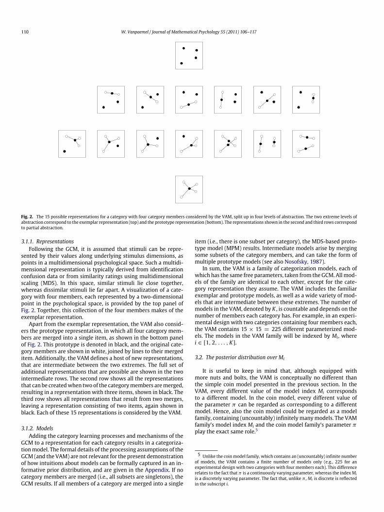
Fig. 2. The 15 possible representations for a category with four category members considered by the VAM, split up in four levels of abstraction. The two extreme levels ofabstraction correspond to the exemplar representation (top) and the prototype representation (bottom). The representations shown in the second and third rows correspondto partial abstraction.

3.1.1. RepresentationsFollowing the GCM, it is assumed that stimuli can be repre-

sented by their values along underlying stimulus dimensions, aspoints in a multidimensional psychological space. Such a multidi-mensional representation is typically derived from identificationconfusion data or from similarity ratings using multidimensionalscaling (MDS). In this space, similar stimuli lie close together,whereas dissimilar stimuli lie far apart. A visualization of a cate-gory with four members, each represented by a two-dimensionalpoint in the psychological space, is provided by the top panel ofFig. 2. Together, this collection of the four members makes of theexemplar representation.

Apart from the exemplar representation, the VAM also consid-ers the prototype representation, in which all four category mem-bers are merged into a single item, as shown in the bottom panelof Fig. 2. This prototype is denoted in black, and the original cate-gory members are shown in white, joined by lines to their mergeditem. Additionally, the VAM defines a host of new representations,that are intermediate between the two extremes. The full set ofadditional representations that are possible are shown in the twointermediate rows. The second row shows all the representationsthat can be createdwhen two of the categorymembers aremerged,resulting in a representation with three items, shown in black. Thethird row shows all representations that result from two merges,leaving a representation consisting of two items, again shown inblack. Each of these 15 representations is considered by the VAM.

3.1.2. ModelsAdding the category learning processes and mechanisms of the

GCM to a representation for each category results in a categoriza-tionmodel. The formal details of the processing assumptions of theGCM (and the VAM) are not relevant for the present demonstrationof how intuitions about models can be formally captured in an in-formative prior distribution, and are given in the Appendix. If nocategory members are merged (i.e., all subsets are singletons), theGCM results. If all members of a category are merged into a single

item (i.e., there is one subset per category), the MDS-based proto-type model (MPM) results. Intermediate models arise by mergingsome subsets of the category members, and can take the form ofmultiple prototype models (see also Nosofsky, 1987).

In sum, the VAM is a family of categorization models, each ofwhich has the same free parameters, taken from the GCM. Allmod-els of the family are identical to each other, except for the cate-gory representation they assume. The VAM includes the familiarexemplar and prototype models, as well as a wide variety of mod-els that are intermediate between these extremes. The number ofmodels in the VAM, denoted by K , is countable and depends on thenumber of members each category has. For example, in an experi-mental design with two categories containing four members each,the VAM contains 15 × 15 = 225 different parameterized mod-els. The models in the VAM family will be indexed by Mi, wherei ∈ [1, 2, . . . , K ].

3.2. The posterior distribution over Mi

It is useful to keep in mind that, although equipped withmore nuts and bolts, the VAM is conceptually no different thanthe simple coin model presented in the previous section. In theVAM, every different value of the model index Mi correspondsto a different model. In the coin model, every different value ofthe parameter π can be regarded as corresponding to a differentmodel. Hence, also the coin model could be regarded as a modelfamily, containing (uncountably) infinitelymanymodels. The VAMfamily’s model index Mi and the coin model family’s parameter πplay the exact same role.5

5 Unlike the coinmodel family, which contains an (uncountably) infinite numberof models, the VAM contains a finite number of models only (e.g., 225 for anexperimental design with two categories with four members each). This differencerelates to the fact that π is a continuously varying parameter, whereas the indexMiis a discretely varying parameter. The fact that, unlike π , Mi is discrete is reflectedin the subscript i.

W. Vanpaemel / Journal of Mathematical Psychology 55 (2011) 106–117 111

Just like the coin model family can be used to infer from ob-served data which value of π is the most probable to have gener-ated the data (or which values ofπ , if the full posterior distributionismaintained), the VAM can be used for estimation—inferring fromobserved datawhich value(s) ofMi (i.e., whichmodel(s) of the VAMfamily) is (are) themost likely to have generated the data. Using theVAM to estimate Mi from data d observed in a category learningtask is conceptually identical to using the coin model to estimateπ from the observed number of heads in a sequence of coin tosses.Estimation proceeds by calculating the posterior distribution,which can be obtained using Bayes’ rule (see (3)). Rather than overπ , the distribution of interest is the posterior distribution overMi:

P(Mi | d) =P(d | Mi)P(Mi)

P(d). (11)

Aswith the coinmodel, the posterior distribution requires three in-gredients. The first is the normalizing constant P(d), which is givenby

P(d) =

K−i=1

P(d | Mi)P(Mi). (12)

The normalizing constant is computed by summation rather thanintegration as in (4), because, unlike π ,Mi is discrete.

The second ingredient to calculate the posterior is the likelihoodP(d | Mi). In the coin tossing example, the likelihood is straightfor-wardly definedby (1). In theVAM, the likelihood is somewhatmorecomplicated. In the coin model family, the model that results at agiven value of π is a parameter-free point hypothesis, and it there-fore makes unambiguous (albeit probabilistic) predictions. In con-trast, in the VAM family, the model that results at a given value ofMi contains free parameters (in particular, the ones adopted fromthe GCM). For a parameterized model as Mi, P(d | Mi) is known asthe marginal likelihood, and it can be obtained by integrating out,or marginalizing over, the parameters (see, e.g., Lee, 2004; Myung& Pitt, 1997):

P(d | Mi) =

∫Ωτ

P(d | τ ,Mi)p(τ | Mi)dτ , (13)

where Ωτ indicates the prior range of the parameter (vector) τ ,p(τ | Mi) indicates the prior distribution over τ , and P(d | τ ,Mi)indicates the likelihood. The range, prior, and likelihood are dis-cussed in the Appendix.

The third part in the calculation of P(Mi | d) is the prior distri-bution P(Mi). One particularly easy, and tomany appealing, way tocompute P(Mi) is to assume equal prior probabilities for all modelsindexed by Mi (i.e., P(Mi) is the uniform distribution). Most cur-rent modeling in psychology, explicitly or most often implicitly,relies on this uniform assumption. However, as illustrated in thecoin tossing example, taking prior knowledge into account in es-timation, in the form of an informative prior distribution, can ad-just implausible estimates and improve inference. In the context ofthe VAM as well, adding prior information through an informativeprior distribution overMi has the desirable effect of smoothing theinferences made by the VAM, by avoiding implausible estimates.

While in the coin tossing example the translation of the expec-tations about π is fairly straightforward, by setting α and β to spe-cific values in (7), this ismuch less so forMi. It is at this pointwherehierarchicalmethods come in useful: as away to formally translatetheory or intuitions into a non-uniform, informative prior distribu-tion over models. The next section illustrates how the hierarchicalintroduction of a theoretically meaningful parameterized genera-tive process, motivated by existing psychological intuitions aboutthe relative plausibilities of the models, naturally gives rise to aninformative prior distribution P(Mi).

4. Constructing an informative prior

Using a hierarchical extension to formally translate theory orintuitions about models in a model family into a prior modeldistribution involves three steps (e.g., Lee, 2006). The first stepinvolves deciding which intuitions and expectations about themodels under consideration seem reasonable. The second step is,inspired by these intuitions, to define a process that generatesthe models. This generative process then automatically imposesa theoretically informed and psychologically meaningful, non-uniform prior distribution over the models. These three steps areillustrated for the VAM, taking the lead from Lee and Vanpaemel(2008).

4.1. Priors intuitions about the models in the VAM family

The first step of the hierarchical extension of the VAM is articu-lating whichmodels are intuitively more likely than others. To thisend, it is useful to note that the models in the VAM family differ intwo aspects. First, they differ in their level of abstraction, roughlyreflected by howmany category members are merged. Second, at agiven level of abstraction, the extreme ones aside, different mod-els are possible, differing inwhichmembers exactly are merged. Inthe present demonstration, two intuitions will be formalized, oneabout each aspect.

As far as the number of merges is concerned, there exists ampleevidence for prototype and exemplar models, suggesting they areviable accounts of category learning. Therefore, these models aregiven a high prior mass, inversely proportional to the number ofabstraction levels implied by the experimental design. As far asthe type of merges is concerned, it seems reasonable to expectthat merging is driven by similarity. Taking the category fruit as anexample, one could sensibly expect that similar members, such astwo different lemons or a lemon and an orange, are merged ratherthan dissimilar members, such as a lemon and a banana. In thecontext of the VAM, the model at the very right end of the secondrow in Fig. 2 seems intuitively more likely than its immediate(left) neighbor. This bias towards similarity is a core assumptionof other models that are similar to the VAM, like SUSTAIN (Loveet al., 2004) and the Rational Model of Categorization (Anderson,1991; Griffiths, Canini, Sanborn, & Navarro, 2007).

4.2. Generating the models in the VAM family

The second step of the hierarchical extension of themodel fam-ily is to capture these prior intuitions in a process for generatingthe models. In this application, the generative process starts withthe exemplar model (at the top of Fig. 2) and, because it is inspiredby two intuitions, it has two parts and two hierarchical parame-ters. How many merges are made – how deep the process contin-ues in Fig. 2 – is controlled by the first part of the process. When anadditional merge is undertaken, different merges are possible, asindicated by the six (or seven) possibilities in the second (or third)row of Fig. 2. Which members are merged – how far to the left orthe right the process continues in Fig. 2 – is controlled by the sec-ond part of the process. Consistent with the intuition that mergingis driven by similarity, the probability of being merged should de-pend on the similarity of the black items (i.e., the original categorymembers or their merged replacement) in a current model.

Formally, the probability that an additional merge will takeplace, and the process will continue, is instantiated by a parameter0 ≤ θ ≤ 1. This means that, at any stage of the process, there is a1− θ probability that the current model will be maintained as thefinal one. If θ is close to 1, merging is very likely, and the prototypemodel almost always results. If, instead, θ is close to 0, merging isvery unlikely, and the exemplar model is almost always retained.

112 W. Vanpaemel / Journal of Mathematical Psychology 55 (2011) 106–117

Further, the probability of choosing to merge the pair of items(i, j) is given by an exponentiated Luce choice rule,

pij =sγij∑

x

∑y≥x

sγxy, (14)

where sij, the similarity between the ith and jth item, is modeledas an exponentially decaying function of the Minkowski r-metricdistance between their points, sij = exp[−

∑k(|vik − vjk|

r)1/r ],with vik the coordinate location on the kth dimension for the pointthat represents the ith item. The parameter γ ≥ 0 controls thelevel of emphasis given to similarity in determining the pair tobe merged. When γ = 0, similarity is not taken into account, soall pairs of items are equally likely to be merged. Since the pairthat is merged is chosen at random, all models within a given levelof abstraction are equally probable. As γ increases, the maximallysimilar pair dominates the others, and will be chosen as the pair tobe merged with probability approaching one. For example, whenγ is very large (e.g., γ = 10), only the most similar items aremerged. This would imply that, in the second row of Fig. 2, themodel to the far right will be the only one that is generated at thatlevel of abstraction. Values of γ between these extremes result inintermediate behavior. In the second row of Fig. 2, themodel to thefar right will be the most likely one, but also other models at thesame level of abstraction will have a non-negligible probability ofbeing generated.

4.3. The prior distribution over the models in the VAM family

The generative process assigns, for each value of θ and γ , aprobability to each of the models in the VAM family, P(Mi | θ, γ ).In the third and final step of the construction of the informativeprior, the prior distribution over Mi is obtained by integrating outthe hierarchical parameters θ and γ , weighted by their prior:

P(Mi) =

∫Ωθ

∫Ωγ

p(Mi | θ, γ )p(θ, γ ) dθ dγ . (15)

Thus themodel prior P(Mi) is the average of all of the distributionsthat result from some combination of θ and γ , weighted by thepriors for θ and γ . In the present applications, θ and γ wereassumed to be independent: i.e., p(θ, γ ) = p(θ)p(γ ). For γ , it wasassumed that

γ ∼ Gamma(2, 1), (16)

which gives support to all positive values, but has most densityaround the modal value one, corresponding to the prior expecta-tion that similarity plays an important role inmerging. For θ , it wasassumed that

θ ∼ Beta(3.2, 1.8). (17)

Consistent with prior intuitions, this distribution assures that theprototype and exemplar models both have a prior mass of roughly16 , reflecting the number of levels of abstraction in an experimentaldesign involving two categories with four members each.6

In sum, the distribution P(Mi) falls out of the way in whichthe generative process works, and the priors on the hierarchicalparameters that control the process. This means that it directlyfollows from theoretical assumptions about how themodels in theVAMare generated, and is fully specified before any data have beenobserved, or inferences have been made.

6 This is the design of seven of the ten data sets considered in the rest of thisarticle. The remaining three data sets involve one category with three membersand another category with four members, and required a Beta(2.4, 1.5) prior for θ ,assigning a prior mass of 1

5 to both the exemplar and prototype models.

5. Application to data from category learning tasks

In this section, the VAM is used to estimate Mi based on tenpreviously published data sets. All data sets were taken fromthree seminal articles presented by Nosofsky and his collaborators(Nosofsky, 1986, 1987; Nosofsky, Clark, & Shin, 1989). The categorylearning tasks involve learning various two-category structuresover a small number of stimuli varying on two dimensions (forexample, color chips varying in saturation and brightness). In eachtask, a subset of the stimuli is assigned to categories A and B,and the remaining stimuli are left unassigned. Most tasks consistof a training phase, in which the category structure is learned,followed by a test phase. During the training phase, only theassigned stimuli are presented, and the participant classifies eachpresented stimulus into either category A or category B. Followingeach response, corrective feedback is presented. During the testphase, both the trained and the untrained stimuli are presented.The human data used in the estimation ofMi are the categorizationresponses to the stimuli presented in the test phase. Some detailsabout these data sets are provided in Table 1.

To illustrate how the hierarchical extension to the VAM andthe informative prior over the models it implies make a differencein the estimation, I focus on two versions of the VAM. Thefirst one, VAMuni, assumes a uniform prior over the models, sothat each model of the VAM is a priori equally likely (formally,P(Mi) =

1K ). The second version is VAMsim, which assumes the

informative prior obtained by the generative process described inthe previous section. According to VAMuni, all levels of abstractionare equally likely, and all sorts of merging are equally likely.VAMsim, in contrast, captures two intuitions: extreme levels ofabstraction are more likely than intermediate ones; similarly-based intermediate models are more likely than intermediatemodels based on the merging of dissimilar category members.

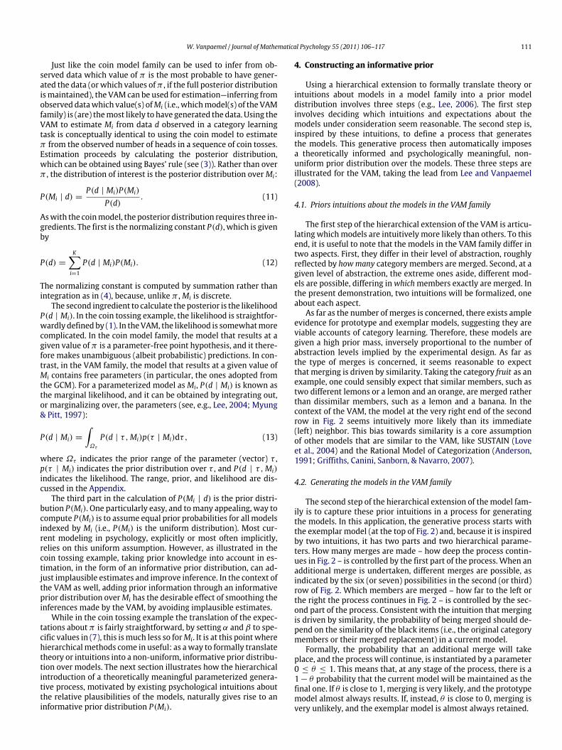
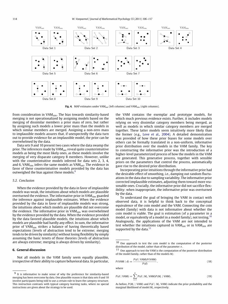
These biases are illustrated in Fig. 3, showing, for data set 6, the13 models with the highest prior mass. The bottom row of Fig. 3shows themodels, using the graphical conventions adopted earlier(i.e., the items representing the category are shown in black andare connected by lines to the original category members, shown inwhite). Squares relate to category A and circles relate to categoryB. The top row of Fig. 3 indicates, by the height of the bar, the priormass the model is given under VAMsim. The four models with thehighest mass, on the left, show the bias towards extreme levels ofabstraction, corresponding to the exemplar model, the prototypemodel, and the two hybrid mixture models where one categoryhas an exemplar representation and the other one has a prototyperepresentation. The remaining nine models show the bias towardssimilarity-basedmerging. Ifmerging takes place, it always involvesstimuli that lie very close, and are thus similar to each other. Forexample, the stimulus represented by the square in the left bottomcorner, which is clearly separated from the three other stimuli inthe same category, is only merged if this merging results in theprototype model.

The aim of the application is to demonstrate the effect ofan informative prior in estimation, rather than providing insightinto category learning. The substantive insights that follow fromthe application of the VAM, as well as the implications for theprototype versus exemplar debate, are discussed elsewhere (Lee& Vanpaemel, 2008; Vanpaemel & Storms, 2008).

5.1. Results

The primary interest concerns the inferences that can be drawnfrom the posterior distribution P(Mi | d).7 As noted earlier, the full

7 Note that the parameter θ can be readily interpreted as a measure of theextent of abstraction, and γ as a measure of the reliance on similarity in forming

W. Vanpaemel / Journal of Mathematical Psychology 55 (2011) 106–117 113

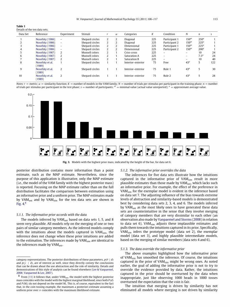
Table 1Details of the ten data sets.

Data Set Reference Experiment Stimuli r α Categories K Condition N n s

1 Nosofsky (1986) – Shepard circles 2 2 Diagonal 225 Participant 1 150m 250a 12 Nosofsky (1986) – Shepard circles 2 2 Diagonal 225 Participant 2 150m 225a 13 Nosofsky (1986) – Shepard circles 2 2 Dimensional 225 Participant 1 150m 225a 14 Nosofsky (1986) – Shepard circles 2 2 Dimensional 225 Participant 2 150m 200a 15 Nosofsky (1987) 2 Munsell colors 2 1 Criss-cross 225 – – 10 246 Nosofsky (1987) 2 Munsell colors 2 1 Saturation A 225 – – 7.5a 247 Nosofsky (1987) 2 Munsell colors 2 1 Saturation B 225 – – 10 408 Nosofsky et al.

(1989)1 Shepard circles 1 1 Interior–exterior 75 Free 43a 5 122

9 Nosofsky et al.(1989)

2 Shepard circles 1 1 Interior–exterior 75 Rule 1 43a 5 30

10 Nosofsky et al.(1989)

2 Shepard circles 1 1 Interior–exterior 75 Rule 2 43a 5 28

Notes: r = metric; α = similarity function; K = number of models in the VAM family; N = number of trials per stimulus per participant in the training phase; n = numberof trials per stimulus per participant in the test phase; s = number of participants; m

= minimal value (actual value unreported); a= approximate average value.

Fig. 3. Models with the highest prior mass, indicated by the height of the bar, for data set 6.

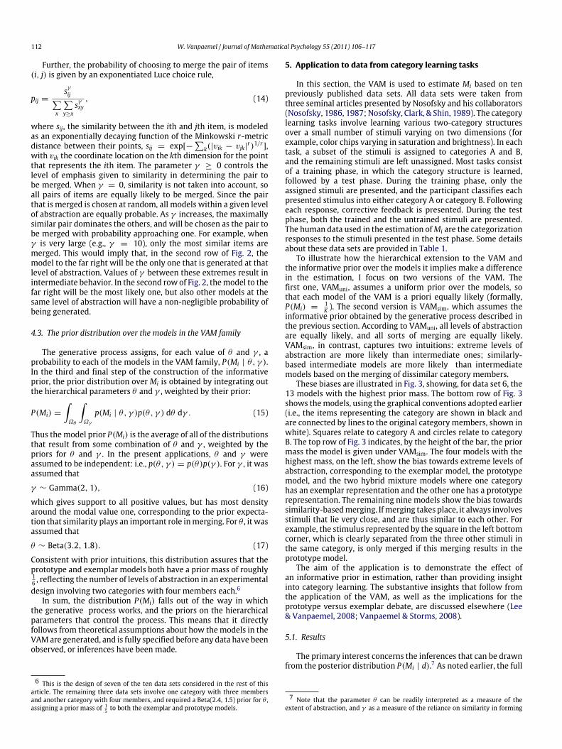
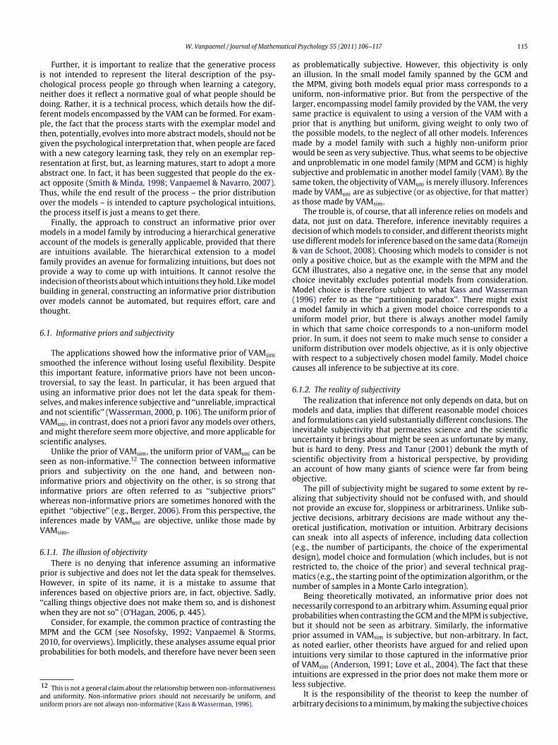
posterior distribution contains more information than a pointestimate, such as the MAP estimate. Nevertheless, since thepurpose of this application is illustrative, only the MAP estimate(i.e., the model of the VAM family with the highest posterior mass)is reported. Focusing on the MAP estimate rather than on the fulldistribution facilitates the comparison between estimation usingan informative prior and a uniform prior. TheMAP estimates madeby VAMuni and by VAMsim for the ten data sets are shown inFig. 4.8

5.1.1. The informative prior accords with the dataThe models inferred by VAMuni based on data sets 1, 5, and 8

seem very plausible. All models rely on the merging of one or twopairs of similar category members. As the inferred models complywith the intuitions about the models captured in VAMsim, theinference does not change when these prior intuitions are addedto the estimation. The inferences made by VAMsim are identical tothe inferences made by VAMuni.

category representations. The posterior distributions of these parameters, p(θ | d)and p(γ | d), are of interest as well, since they directly convey the conclusionsthat can be drawn about the use abstraction and the role of similarity. Details anddemonstrations of this style of analysis can be found elsewhere (Lee & Vanpaemel,2008; Vanpaemel & Lee, 2007).8 From (11) it follows that, under VAMuni , the model with the highest posterior

mass coincideswith themodelwith the highestmarginal likelihood, since both P(d)and P(Mi) do not depend on the model Mi . This is, of course, equivalent to the factthat, in the coin tossing example, the maximum a posteriori estimate assuming auniform prior over π coincides with the maximum likelihood estimate.

5.1.2. The informative prior overrides the dataThe inferences for five data sets illustrate how the intuitions

captured in the informative prior of VAMsim result in moreplausible estimates than those made by VAMuni, which lacks suchan informative prior. For example, the effect of the preference inVAMsim for the exemplar model is evident in the inference basedon data set 7. The adjusting influence of the bias towards extremelevels of abstraction and similarity-based models is demonstratedbest by considering data sets 2, 3, 4, and 6. The models inferredby VAMuni as the most likely ones to have generated these datasets are counterintuitive in the sense that they involve mergingof category members that are very dissimilar to each other (anobservation alsomade byVanpaemel and Storms (2008) in relationto data set 6). VAMsim adjusts these implausible estimates andpulls them towards the intuitions captured in its prior. Specifically,VAMsim infers the prototype model (data set 2), the exemplarmodel (data set 3), and highly plausible intermediate models,based on the merging of similar members (data sets 4 and 6).

5.1.3. The data override the informative priorThe above examples highlighted how the informative prior

of VAMsim has smoothed the inference. Of course, the intuitionscaptured in the prior of VAMsim might be wrong ones. As notedearlier, the goal of adding the informative prior is not to try tooverride the evidence provided by data. Rather, the intuitionscaptured in the prior should be overturned by the data wheninappropriate, just like observing 1000 heads in 1000 tossesoverturned the expectation that the coin is fair.

The intuition that merging is driven by similarity has noteliminated all models where merging is not driven by similarity

114 W. Vanpaemel / Journal of Mathematical Psychology 55 (2011) 106–117

Fig. 4. MAP estimates under VAMuni (left columns) and VAMsim (right columns).

from consideration in VAMsim. The bias towards similarity-basedmerging is not operationalized by assigning models based on themerging of dissimilar members a prior mass of zero, but ratherby assigning such models a lower prior mass than the models inwhich similar members are merged. Assigning a non-zero massto implausible models assures that, if unexpectedly the data turnout to provide evidence for an implausible model, the prior can beoverwhelmed by the data.

Data sets 9 and 10 present two cases where the data swamp theprior. The inferencesmade by VAMuni reveal quite counterintuitivemodels as being the most likely ones, as these models involve themerging of very disparate category B members. However, unlikewith the counterintuitive models inferred for data sets 2, 3, 4,and 6, VAMsim infers the same models as VAMuni. The evidence infavor of these counterintuitive models provided by the data hasoutweighed the bias against these models.9

5.2. Conclusion

When the evidence provided by the data in favor of implausiblemodels was weak, the intuitions about whichmodels are plausibleoverturned the evidence. The informative prior in VAMsim guardedthe inference against implausible estimates. When the evidenceprovided by the data in favor of implausible models was strong,the intuitions about which models are plausible did not overcomethe evidence. The informative prior in VAMsim was overwhelmedby the evidence provided by the data.When the evidence providedby the data favored plausible models, the intuitions about whichmodels are plausible had hardly any effect. In sum, the informativeprior of VAMsim strikes a balance of having theoretically basedexpectations (levels of abstraction tend to be extreme; mergingtends to be driven by similarity)without losing flexibility by simplyassuming the basic tenets of those theories (levels of abstractionare always extreme; merging is always driven by similarity).

6. General discussion

Not all models in the VAM family seem equally plausible,irrespective of their ability to capture behavioral data. In particular,

9 It is informative to make sense of why the preference for similarity-basedmerging has been overcome by data. One plausible reason is that data sets 9 and 10involve participants being told to use a certain rule to learn the category structure.This instruction contrasts with typical category learning tasks, where no specialinstructions are given about the strategy to be used.

the VAM contains the exemplar and prototype models, forwhich much previous evidence exists. Further, it includes modelsrelying on very dissimilar category members being merged, aswell as models in which similar category members are mergedtogether. These latter models seem intuitively more likely thanthe former (e.g., Love et al., 2004). A detailed demonstrationwas provided of how these prior biases for some models overothers can be formally translated in a non-uniform, informativeprior distribution over the models in the VAM family. The keyto constructing the informative prior was the introduction of ahigher-level parameterized process of how the models in the VAMare generated. This generative process, together with sensiblepriors on the parameters that control the process, automaticallygave rise to the desired prior distribution.

Incorporating prior intuitions through the informative prior hadthe desirable effect of smoothing, i.e., damping out random fluctu-ations in the data due to sampling variability. The informative priorcorrected implausible estimates, adjusting them towardmore rea-sonable ones. Crucially, the informative prior did not sacrifice flex-ibility: when inappropriate, the informative prior was overturnedby the data.

To understand the goal of bringing the VAM in contact withobserved data, it is helpful to think back to the conceptualequivalence of the coin model and the VAM. Connecting the coinmodel (family) with data is not informative about whether thecoin model is viable. The goal is estimation (of a parameter in amodel, or equivalently of a model in a model family), not testing.10Analogously, the applications of the VAM are not intended totest whether the intuitions captured in VAMuni or in VAMsim aresupported by the data.11

10 One approach to test the coin model is the computation of the posteriordistribution of the model, rather than of the parameter π .11 One approach to test the VAM is the computation of the posterior distributionof the model family, rather than of the models Mi:

P(VAM | d) =P(d | VAM)P(VAM)

P(d), (18)

where

P(d | VAM) =

K−i=1

P(d | Mi,VAM)P(Mi | VAM). (19)

As before, P(Mi | VAM) and P(d | Mi,VAM) indicate the prior probability and themarginal likelihood of model Mi , respectively.

W. Vanpaemel / Journal of Mathematical Psychology 55 (2011) 106–117 115

Further, it is important to realize that the generative processis not intended to represent the literal description of the psy-chological process people go through when learning a category,neither does it reflect a normative goal of what people should bedoing. Rather, it is a technical process, which details how the dif-ferent models encompassed by the VAM can be formed. For exam-ple, the fact that the process starts with the exemplar model andthen, potentially, evolves intomore abstract models, should not begiven the psychological interpretation that, when people are facedwith a new category learning task, they rely on an exemplar rep-resentation at first, but, as learning matures, start to adopt a moreabstract one. In fact, it has been suggested that people do the ex-act opposite (Smith & Minda, 1998; Vanpaemel & Navarro, 2007).Thus, while the end result of the process – the prior distributionover the models – is intended to capture psychological intuitions,the process itself is just a means to get there.

Finally, the approach to construct an informative prior overmodels in a model family by introducing a hierarchical generativeaccount of the models is generally applicable, provided that thereare intuitions available. The hierarchical extension to a modelfamily provides an avenue for formalizing intuitions, but does notprovide a way to come up with intuitions. It cannot resolve theindecision of theorists aboutwhich intuitions theyhold. Likemodelbuilding in general, constructing an informative prior distributionover models cannot be automated, but requires effort, care andthought.

6.1. Informative priors and subjectivity

The applications showed how the informative prior of VAMsimsmoothed the inference without losing useful flexibility. Despitethis important feature, informative priors have not been uncon-troversial, to say the least. In particular, it has been argued thatusing an informative prior does not let the data speak for them-selves, andmakes inference subjective and ‘‘unreliable, impracticaland not scientific’’ (Wasserman, 2000, p. 106). The uniform prior ofVAMuni, in contrast, does not a priori favor anymodels over others,and might therefore seemmore objective, and more applicable forscientific analyses.

Unlike the prior of VAMsim, the uniform prior of VAMuni can beseen as non-informative.12 The connection between informativepriors and subjectivity on the one hand, and between non-informative priors and objectivity on the other, is so strong thatinformative priors are often referred to as ‘‘subjective priors’’whereas non-informative priors are sometimes honored with theepithet ‘‘objective’’ (e.g., Berger, 2006). From this perspective, theinferences made by VAMuni are objective, unlike those made byVAMsim.

6.1.1. The illusion of objectivityThere is no denying that inference assuming an informative

prior is subjective and does not let the data speak for themselves.However, in spite of its name, it is a mistake to assume thatinferences based on objective priors are, in fact, objective. Sadly,‘‘calling things objective does not make them so, and is dishonestwhen they are not so’’ (O’Hagan, 2006, p. 445).

Consider, for example, the common practice of contrasting theMPM and the GCM (see Nosofsky, 1992; Vanpaemel & Storms,2010, for overviews). Implicitly, these analyses assume equal priorprobabilities for both models, and therefore have never been seen

12 This is not a general claim about the relationship between non-informativenessand uniformity. Non-informative priors should not necessarily be uniform, anduniform priors are not always non-informative (Kass & Wasserman, 1996).

as problematically subjective. However, this objectivity is onlyan illusion. In the small model family spanned by the GCM andthe MPM, giving both models equal prior mass corresponds to auniform, non-informative prior. But from the perspective of thelarger, encompassing model family provided by the VAM, the verysame practice is equivalent to using a version of the VAM with aprior that is anything but uniform, giving weight to only two ofthe possible models, to the neglect of all other models. Inferencesmade by a model family with such a highly non-uniform priorwould be seen as very subjective. Thus, what seems to be objectiveand unproblematic in one model family (MPM and GCM) is highlysubjective and problematic in another model family (VAM). By thesame token, the objectivity of VAMuni is merely illusory. Inferencesmade by VAMuni are as subjective (or as objective, for that matter)as those made by VAMsim.

The trouble is, of course, that all inference relies on models anddata, not just on data. Therefore, inference inevitably requires adecision ofwhichmodels to consider, and different theoristsmightuse differentmodels for inference based on the samedata (Romeijn& van de Schoot, 2008). Choosing which models to consider is notonly a positive choice, but as the example with the MPM and theGCM illustrates, also a negative one, in the sense that any modelchoice inevitably excludes potential models from consideration.Model choice is therefore subject to what Kass and Wasserman(1996) refer to as the ‘‘partitioning paradox’’. There might exista model family in which a given model choice corresponds to auniform model prior, but there is always another model familyin which that same choice corresponds to a non-uniform modelprior. In sum, it does not seem to make much sense to consider auniform distribution over models objective, as it is only objectivewith respect to a subjectively chosen model family. Model choicecauses all inference to be subjective at its core.

6.1.2. The reality of subjectivityThe realization that inference not only depends on data, but on

models and data, implies that different reasonable model choicesand formulations can yield substantially different conclusions. Theinevitable subjectivity that permeates science and the scientificuncertainty it brings about might be seen as unfortunate by many,but is hard to deny. Press and Tanur (2001) debunk the myth ofscientific objectivity from a historical perspective, by providingan account of how many giants of science were far from beingobjective.

The pill of subjectivity might be sugared to some extent by re-alizing that subjectivity should not be confused with, and shouldnot provide an excuse for, sloppiness or arbitrariness. Unlike sub-jective decisions, arbitrary decisions are made without any the-oretical justification, motivation or intuition. Arbitrary decisionscan sneak into all aspects of inference, including data collection(e.g., the number of participants, the choice of the experimentaldesign), model choice and formulation (which includes, but is notrestricted to, the choice of the prior) and several technical prag-matics (e.g., the starting point of the optimization algorithm, or thenumber of samples in a Monte Carlo integration).

Being theoretically motivated, an informative prior does notnecessarily correspond to an arbitrarywhim. Assuming equal priorprobabilitieswhen contrasting theGCMand theMPM is subjective,but it should not be seen as arbitrary. Similarly, the informativeprior assumed in VAMsim is subjective, but non-arbitrary. In fact,as noted earlier, other theorists have argued for and relied uponintuitions very similar to those captured in the informative priorof VAMsim (Anderson, 1991; Love et al., 2004). The fact that theseintuitions are expressed in the prior does not make them more orless subjective.

It is the responsibility of the theorist to keep the number ofarbitrary decisions to aminimum, bymaking the subjective choices

116 W. Vanpaemel / Journal of Mathematical Psychology 55 (2011) 106–117

non-arbitrary and well motivated. Further, where possible, therobustness of the conclusions against any arbitrary decision thatwas impossible to avoid should be checked. Finally, given thatsubjectivity permeates all aspects of science, it is essential to makesure that all subjectivity is transparent, fully in view, and availablefor scrutiny. It speaks for the informative Bayesian approach that itmakes (part of) the inevitable subjectivity explicit and precise, incontrast to many non-Bayesian approaches relying on implicit anddefault assumptions.

6.2. Model expansion and extension

In many debates in psychology, progress is sought by develop-ing a limited number ofmodels that adopt different theoretical po-sitions, and evaluating these models on the basis of empirical data.These evaluations then lead to choosing one model to the exclu-sion of all others. Considering a limited number of possibilities onlyprovides a narrow window on the possible ways in which peoplecan engage in a task. Expanding the number of theoretical posi-tions results in a freshening broadening of the debate, a strategyknown as model expansion in statistics (see, e.g., Draper, 1995).Using a largemodel family rather than a limited set ofmodels facil-itates approaching the debate fromamodel estimation perspectiverather than from a model selection perspective.

The hierarchical extension to a model family demonstrated inthis article seems to be most valuable for the areas of modeling inpsychology where the few models typically considered can be orhave been sensibly expanded into a broader model family. Havingexpanded the models into a large model family, the hierarchicalextension has the ability to generate psychologically meaningful,informative priors over the models and to tie the models togetherat a higher level in the hierarchy. Jointly, the vertical expansionand the horizontal hierarchical extension can result in a rich andpowerful estimation tool that can be used to advance and deepenour understanding.

Acknowledgments

The research reported in this article was funded by Grant FWOG.0513.08. I wish to thank Gert Storms for his support, Jan-WillemRomeijn for his insightful and detailed comments, andMichael Leefor both.

Appendix. Formal details of the GCM and the VAM

In the experimental designs considered in this article, stimuliare represented as points in a two-dimensional space. Let pikdenote the coordinate location on the kth dimension for the pointthat represents the ith stimulus presented in the test phase. Let vikdenote the coordinate location on the kth dimension for the pointthat represents the ith category member. The assignment of thecategorymembers to the two categories, as defined by the categorystructure to be learned, is represented by indicator variables, sothat ai = 1 if the ith category member belongs to category A, andai = 0 otherwise.

The response probability for the ith test stimulus being chosenas amember of category A is determined by the similarity betweenthe stimulus and both categories, according to a Luce choice rule13

ri =siA

siA + siB. (20)

13 A more general response rule with two additional parameters, the bias κ

and the response scaling λ, has also been proposed: ri =κsλiA

κsλiA+(1−κ)sλiB(Ashby &

Maddox, 1993; Navarro, 2007). This more general form is not used in the presentapplications.

In the GCM, siA, the similarity between the ith test stimulus andcategory A, is computed by the sum of the similarities between thestimulus and all members of category A:

siA =

−j

ajsij, (21)

and similarly

siB =

−j

(1 − aj)sij, (22)

where j indexes all category members. The similarity between theith test stimulus and the jth category member, sij, is modeled as anexponentially decaying function of their distance, dij:

sij = exp−(cdij)α, (23)

where c is the sensitivity parameter measuring the rate at whichsimilarity declines with distance, and α determines the shape ofthe function. The distance between the ith test stimulus and thejth category member is calculated according to the Minkowski r-metric:

drij = w(pi1 − vj1)r+ (1 − w)(pi2 − vj2)

r , (24)

where w is the attention weight parameter measuring the relativeemphasis given to the first stimulus dimension over the second.

The only way in which the VAM differs from the GCM is thatit does not assume that a category is necessarily represented by thecategorymembers, but also considers other representations. Theserepresentations are formed by merging subsets (possibly single-tons) of category members. This means that the representationsconsidered in the VAM are made up of items that can correspondto the original category members, but also to the merged replace-ments of the category members (i.e., the black circles in Fig. 2).Formally, then, the similarity between a test stimulus and a cat-egory is computed as the sum of the similarities of that stimulus tothe items in the VAM category representation, rather than to thecategorymembers. This implies that ai represents themembershipof the items rather than of the category members, that in (21) and(22) the index j runs over the items rather than over the categorymembers, and that in (24) vik denotes the coordinate location onthe kth dimension for the point that represents the ith item, ratherthan the ith category member.

The present applications relied on the Binomial likelihood

ki ∼ Binomial(ti, ri), (25)

with ki the number of times the ith test stimulus was chosen incategory A and ti the number of times it was presented, and on thefollowing priors for w and c:

w ∼ Uniform (0, 1), (26)

and

c2 ∼ Gamma (ε, ε), (27)

with ε = .001 set near zero, with the range of c being restricted torun between 0 and 10.

References

Anderson, J. R. (1991). The adaptive nature of human categorization. PsychologicalReview, 98, 409–429.

Ashby, F. G., & Maddox, W. T. (1993). Relations between prototype, exemplar, anddecision boundmodels of categorization. Journal ofMathematical Psychology, 37,372–400.

Berger, J. O. (2006). The case for objective Bayesian analysis. Bayesian Analysis, 1,385–402.

Brooks, L. R. (1978). Non-analytic concept formation andmemory for instances. In E.Rosch, & B. B. Lloyd (Eds.), Cognition and categorization (pp. 169–211). Hillsdale,NJ: Lawrence Erlbaum.

Diaconis, P., & Ylvisaker, D. (1979). Conjugate priors for exponential families. TheAnnals of Statistics, 7, 269–281.

W. Vanpaemel / Journal of Mathematical Psychology 55 (2011) 106–117 117

Draper, D. (1995). Assessment and propagation of model uncertainty. Journal of theRoyal Statistical Society. Series B, 57, 45–97.

Efron, B. (1986). Why isn’t everyone a Bayesian? The American Statistician, 40, 1–5.Goldstein, M. (2006). Subjective Bayesian analysis: principles and practice. Bayesian

Analysis, 1, 403–420.Griffiths, T. L., Canini, K. R., Sanborn, A. N., & Navarro, D. J. (2007). Unifying

rational models of categorization via the hierarchical Dirichlet process. In D. S.McNamara, & J. G. Trafton (Eds.), Proceedings of the 29th annual conference of thecognitive science society (pp. 323–328). Austin, TX: Cognitive Science Society.

Griffiths, T. L., Kemp, C., & Tenenbaum, J. B. (2008). Bayesian models of cognition.In R. Sun (Ed.), Cambridge handbook of computational cognitive modeling(pp. 59–100). Cambridge: Cambridge University Press.

Kass, R. E., & Wasserman, L. (1996). The selection of prior distributions by formalrules. Journal of the American Statistical Association, 91, 1343–1370.

Lee, M. D. (2004). A Bayesian analysis of retention functions. Journal of MathematicalPsychology, 48, 310–321.

Lee, M. D. (2006). A hierarchical Bayesian model of human decision-making on anoptimal stopping problem. Cognitive Science, 30, 555–580.

Lee, M. D., & Vanpaemel, W. (2008). Exemplars, prototypes, similarities and rules incategory representation: an example of hierarchical Bayesian analysis. CognitiveScience, 32, 1403–1424.

Lee,M. D., &Wagenmakers, E. J. (2005). Bayesian statistical inference in psychology:comment on Trafimow (2003). Psychological Review, 112, 662–668.

Lindley, D. V. (2004). That wretched prior. Significance, 1, 85–87.Lindley, D. V., & Phillips, L. D. (1976). Inference for a Bernoulli process (a Bayesian

view). The American Statistician, 30, 112–119.Love, B. C., Medin, D. L., & Gureckis, T. M. (2004). SUSTAIN: a network model of

category learning. Psychological Review, 111, 309–332.Medin, D. L., & Schaffer, M. M. (1978). Context theory of classification learning.

Psychological Review, 85, 207–238.Minda, J. P., & Smith, J. D. (2001). Prototypes in category learning: the effects

of category size, category structure, and stimulus complexity. Journal ofExperimental Psychology: Learning, Memory, and Cognition, 27, 775–799.

Morey, R. (2011). A Bayesian hierarchical model for the measurement of workingmemory capacity. Journal of Mathematical Psychology, 55(1), 8–24.

Murphy, G. L. (2002). The big book of concepts. Boston, MA: MIT Press.Myung, I. J., & Pitt, M. A. (1997). Applying Occam’s razor in modeling cognition: a

Bayesian approach. Psychonomic Bulletin & Review, 4, 79–95.Navarro, D. J. (2007). On the interaction between exemplar-based concepts and a

response scaling process. Journal of Mathematical Psychology, 51, 85–98.Nosofsky, R. M. (1984). Choice, similarity, and the context theory of classification.

Journal of Experimental Psychology: Learning, Memory, and Cognition, 10,104–114.

Nosofsky, R. M. (1986). Attention, similarity, and the identification–categorizationrelationship. Journal of Experimental Psychology: General, 115, 39–57.

Nosofsky, R. M. (1987). Attention and learning processes in the identification andcategorization of integral stimuli. Journal of Experimental Psychology: Learning,Memory, and Cognition, 13, 87–108.

Nosofsky, R. M. (1992). Exemplars, prototypes, and similarity rules. In A. F. Healy, S.M. Kosslyn, & R. M. Shiffrin (Eds.), From learning theory to connectionist theory:essays in honor of William K. Estes: vol. 1 (pp. 149–167). Hillsdale, NJ: LawrenceErlbaum.

Nosofsky, R. M., Clark, S. E., & Shin, H. J. (1989). Rules and exemplarsin categorization, identification, and recognition. Journal of ExperimentalPsychology: Learning, Memory, and Cognition, 15, 282–304.

O’Hagan, A. (2006). Science, subjectivity and software (comment on articles byBerger and by Goldstein). Bayesian Analysis, 1, 445–450.

Press, S. J., & Tanur, J. M. (2001). The subjectivity of scientists and the Bayesianapproach. New York: Wiley-Interscience.

Reed, S. K. (1972). Pattern recognition and categorization. Cognitive Psychology, 3,392–407.

Romeijn, J.-W., & van de Schoot, R. (2008). A philosopher’s view on Bayesianevaluation of informative hypotheses. In H. Hoijtink, I. Klugkist, & P. A. Boelen(Eds.), Bayesian evaluation of informative hypotheses (pp. 329–357). New York:Springer.

Rouder, J. N., Lu, J., Speckman, P., Sun, D., & Jiang, Y. (2005). A hierarchical modelfor estimating response time distributions. Psychonomic Bulletin & Review, 12,195–223.

Smith, E. E., & Medin, D. L. (1981). Categories and concepts. Cambridge, MA: HarvardUniversity Press.

Smith, J. D., &Minda, J. P. (1998). Prototypes in themist: the early epochs of categorylearning. Journal of Experimental Psychology: Learning,Memory, and Cognition, 24,1411–1436.

Vanpaemel,W., & Lee,M.D. (2007). Amodel of building representations for categorylearning. In D. S. McNamara, & J. G. Trafton (Eds.), Proceedings of the 29th annualconference of the cognitive science society (pp. 1605–1610). Austin, TX: CognitiveScience Society.

Vanpaemel, W., & Navarro, D. J. (2007). Representational shifts during categorylearning. In D. S. McNamara, & J. G. Trafton (Eds.), Proceedings of the 29th annualconference of the cognitive science society (pp. 1599–1604). Austin, TX: CognitiveScience Society.

Vanpaemel,W., & Storms, G. (2008). In search of abstraction: the varying abstractionmodel of categorization. Psychonomic Bulletin & Review, 15, 732–749.

Vanpaemel, W., & Storms, G. (2010). Abstraction and model evaluation in categorylearning. Behavior Research Methods, 42, 421–437.

Wagenmakers, E. J., Lee,M. D., Lodewyckx, T., & Iverson, G. J. (2008). Bayesian versusfrequentist inference. In H. Hoijtink, I. Klugkist, & P. A. Boelen (Eds.), Bayesianevaluation of informative hypotheses (pp. 181–207). New York: Springer.

Wasserman, L. (2000). Bayesian model selection and model averaging. Journal ofMathematical Psychology, 44, 92–107.