Constructing Basic Galactic Models

Julien Chemouni BachGalactic Ecosystems (AST-193)

Tufts University

December, 2007

Abstract

This paper presents an overview of galactic dynamics that focuses on mathematicaland conceptual modeling of stellar systems at an introductory level. We outline thebasic concepts and assumptions required to build galactic models and then we proceedwith a description of the mathematical methods used, along with an analysis of eachmodel, including results, issues, shortcomings, and comparison with observational data.This paper mixes both qualitative and quantitative accounts of galactic modeling,depending on the complexity of the galactic configuration. In the end, the reader willhave learned the tools required and methods of approach used to construct galaxymodels. We pay particular attention to spherical systems, whose mathematics arerelatively simple, and derive several models. We then turn to axisymmetric and triaxialsystems, dealing with them at a more superficial level. We conclude our study of modelswith spiral systems, the most difficult to model. Finally, we end with an overview ofstability analysis and additional effects not taken into account in our earlier modelingprocedures.

1

‘

Contents

1 Introduction 31.1 Features and Assumptions . . . . . . . . . . . . . . . . . . . . . . . . . . . . 4

2 Constructing a Galaxy 5

3 Spherical Systems 83.1 Spherical Models in Equilibria . . . . . . . . . . . . . . . . . . . . . . . . . . 8

3.1.1 Spherical Systems . . . . . . . . . . . . . . . . . . . . . . . . . . . . 83.1.2 Singular Isothermal Sphere . . . . . . . . . . . . . . . . . . . . . . . 103.1.3 King Models . . . . . . . . . . . . . . . . . . . . . . . . . . . . . . . 15

3.2 Alternate Spherical Models . . . . . . . . . . . . . . . . . . . . . . . . . . . 183.2.1 deVaucouleurs and Sersic Laws . . . . . . . . . . . . . . . . . . . . . 183.2.2 Hubble-Reynolds Law . . . . . . . . . . . . . . . . . . . . . . . . . . 193.2.3 Other Models . . . . . . . . . . . . . . . . . . . . . . . . . . . . . . . 19

4 Axisymmetric Systems 22

5 Triaxial Systems 235.1 Overview . . . . . . . . . . . . . . . . . . . . . . . . . . . . . . . . . . . . . 235.2 Bars . . . . . . . . . . . . . . . . . . . . . . . . . . . . . . . . . . . . . . . . 23

6 Spiral Systems 256.1 Density Wave Kinematics . . . . . . . . . . . . . . . . . . . . . . . . . . . . 256.2 Results of Density Wave Modeling . . . . . . . . . . . . . . . . . . . . . . . 256.3 Remaining Problems . . . . . . . . . . . . . . . . . . . . . . . . . . . . . . . 266.4 Sources of Density Waves . . . . . . . . . . . . . . . . . . . . . . . . . . . . 26

7 Stability 287.1 Choice of Equilibrium . . . . . . . . . . . . . . . . . . . . . . . . . . . . . . 287.2 General Stability . . . . . . . . . . . . . . . . . . . . . . . . . . . . . . . . . 29

7.2.1 Jeans Instability . . . . . . . . . . . . . . . . . . . . . . . . . . . . . 297.3 Stability of Spherical Systems . . . . . . . . . . . . . . . . . . . . . . . . . . 317.4 Stability of Uniformly Rotating Systems . . . . . . . . . . . . . . . . . . . . 317.5 Stability of Disks . . . . . . . . . . . . . . . . . . . . . . . . . . . . . . . . . 32

8 Incorporating Collisions and Other Effects 32

2

1 Introduction

Galaxies are the building blocks of our universe. Home to billions of stars, galaxies comein a variety of shapes and colors, and it is only in the last century that we have begun tounderstand the complex machinery of these grand structures. A variety of dynamical andchemical processes are observed in galaxies that often differ from one to the other. Thus, inorder to fully describe galaxies we require nearly every branch of physics. Galaxies cannotjust be thought of as collections of stars, like atoms in an object. They continually evolveunder the constant influence of physical laws both known and unknown, and as such, theypresent us with a view of nature at its fullest.

The study of galactic stability and equilibria is of the utmost importance in analyzinggalactic dynamics. Equilibrium refers to the state of a stellar system in which all theforces and torques on each star sum to zero. This state corresponds to a sort of finalstate of a galaxy, a structural condition that the galaxy will naturally evolve towardsbased on a variety of initial parameters and ongoing stellar events. For example, a rapidlyspinning sphere will tend to flatten itself into a disk - its equilibrium state. The study ofequilibria is thus extremely useful in theorizing the evolution and initial stages of galaxies.However, there is the crucial question of whether these equilibria are sufficiently stableto correspond to real stellar systems. That is where stability analysis enters in. Anystellar configurations based on equilibrium models must be tested for stability before beingemployed as a realistic model. Looking at our earlier example, a self-gravitating disk inwhich stars move in circular orbits is extremely unstable. The slightest perturbation to thissystem will cause it to quickly move away from this equilibrium state, revealing to us thatin order for a galaxy to form into a disk and remain stable, a minimum level of randommotion is required. Thus, the study of galactic stability helps us modify our models ofgalaxy structure so that they meet the observed structures and dynamics.

The primary goal in the field of galactic dynamics is to come up with a galactic modelthat accurately represents the observed state of a galaxy. Perturbations change galacticstructure drastically and so our basic models must be continuously modified, and in fact,it is the inclusion of these irregularities that allow us to discover where features like spiralarms and bars come from. The analysis of galactic stability and equilibria allows us to notonly describe the current dynamical conditions of a galaxy, but also its past and futureevolution, which would otherwise be impossible for us to observe in our lifetimes. Thus,comparison of our models with real observations provides us with a way of validating theoryand the underlying physical principles behind the analysis.

The study of galactic stability and equilibria is an extremely difficult and complex task,both mathematically and logistically. In fact, one of the most challenging tasks is obtaininghigh quality data from observed stellar systems. In this paper we will focus on relativelysimple models (that can be compared with some readily available and accurate data) withlimited reference to more complicated and comprehensive models. We hope to provide anoverview of the subject from an introductory level and draw more general conclusions on

3

galactic evolution from this foundation. But first, we describe several key characteristicsof galaxies that we will need to keep in mind throughout this paper.

1.1 Features and Assumptions

A galaxy is an enormous collection of gravitationally bound stars—on the order of 106 to1012 stars—that we call a stellar system . And within this stellar system are smaller stellarsystems that create their own local structures, ranging in size from two stars in a binarysystem to millions in a cluster. The end result is an intricate coordination of systemsdominated by Newtonian gravity. Unfortunately for us, the timescale of galactic motionand evolution is so long that our picture of a galaxy is essentially a snapshot in its lifetime.Binney and Tremaine, in their book on Galactic Dynamics (1999), show that the orbitalperiod around the galactic center of stars near the Sun is a factor 105 or 106 times longerthan the interval over which we have recorded observations. We can obtain measurementsof proper motions and line-of-sight velocities of many stars. However, these measurementsgive no indication of acceleration (due to the timescale of this acceleration) and are lessreliable, and often impossible, for far away stars.

Additionally, Binney & Tremaine (1999) calculate the mean free path of a star beforeit collides with another star, finding the collision interval to be on the order of 1019 years1,many times longer than the age of the universe. Thus, collisions between stars are sorare that they do not contribute to the overall dynamics of galaxies and, consequently, thespatial separation of stars means that they can often be regarded as point masses.

From these findings we can draw two key assumptions that will be used throughout thispaper. Firstly, since direct stellar collisions are so rare, each star’s motion is determinedonly by the gravitational attraction of all the other stars in the galaxy. We say that thegalaxy is self-consistent in that the combined mass of the stars provides the densitydistribution that generates the gravitational potential. This assumption will allow us tocreate our first basic mathematical model of galaxies described in Section 3. Our secondassumption is that a galaxy is stationary, meaning that the density at each point isconstant in time because the arrivals and departures of stars in any volume element exactlybalance. The use of this assumption to create models of galaxies implies a galaxy that ismany revolutions old2, and hence in a steady state. We must be careful in our use of thisassumption since many stationary systems are unstable. A small deviation from such amathematical model will cause the system—a galaxy in our case—to evolve away from ourmodel.

1Taking the random velocity of a star to be 40km s−1.2Meaning orbital periods of stars around the galaxy

4

2 Constructing a Galaxy

Describing the dynamics of a galaxy is a daunting task that compels us to begin with themost basic of physical principles. We outline the method behind this subject:

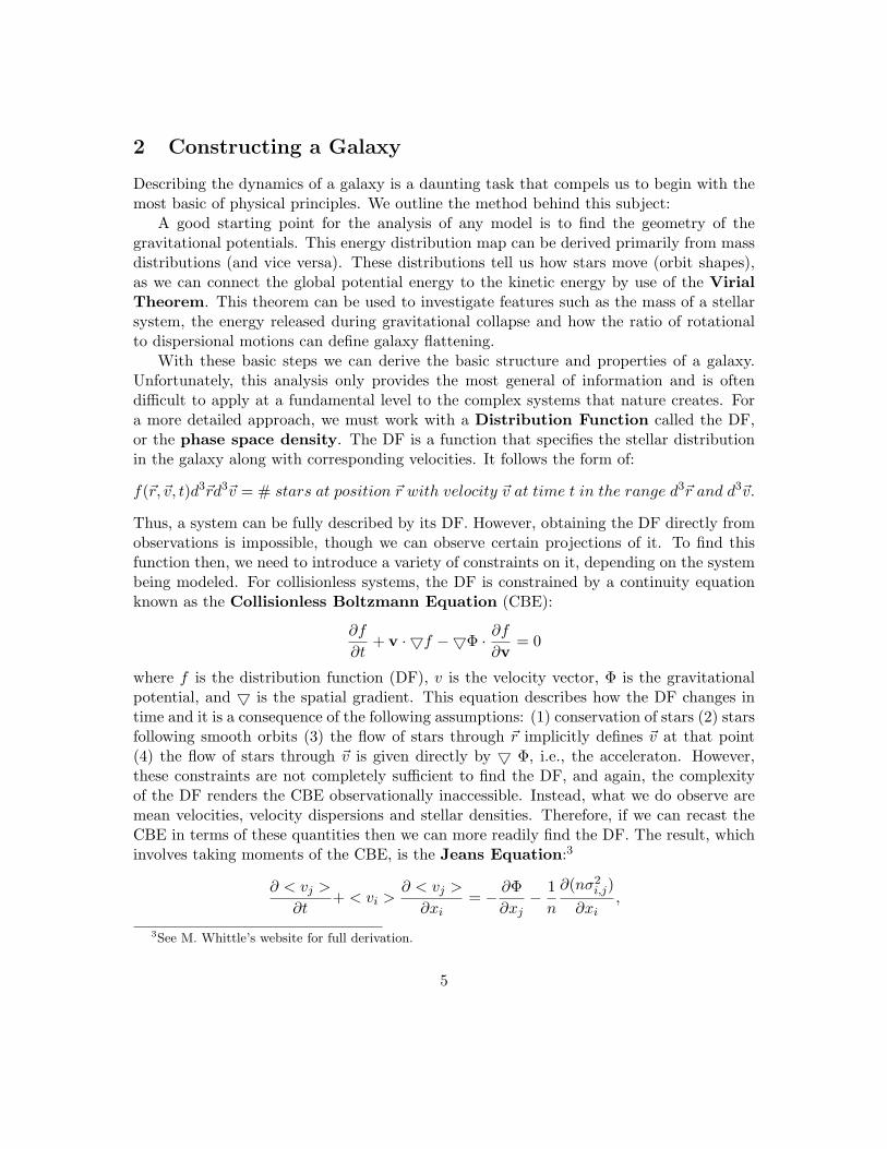
A good starting point for the analysis of any model is to find the geometry of thegravitational potentials. This energy distribution map can be derived primarily from massdistributions (and vice versa). These distributions tell us how stars move (orbit shapes),as we can connect the global potential energy to the kinetic energy by use of the VirialTheorem. This theorem can be used to investigate features such as the mass of a stellarsystem, the energy released during gravitational collapse and how the ratio of rotationalto dispersional motions can define galaxy flattening.

With these basic steps we can derive the basic structure and properties of a galaxy.Unfortunately, this analysis only provides the most general of information and is oftendifficult to apply at a fundamental level to the complex systems that nature creates. Fora more detailed approach, we must work with a Distribution Function called the DF,or the phase space density. The DF is a function that specifies the stellar distributionin the galaxy along with corresponding velocities. It follows the form of:

f(~r,~v, t)d3~rd3~v = # stars at position ~r with velocity ~v at time t in the range d3~r and d3~v.

Thus, a system can be fully described by its DF. However, obtaining the DF directly fromobservations is impossible, though we can observe certain projections of it. To find thisfunction then, we need to introduce a variety of constraints on it, depending on the systembeing modeled. For collisionless systems, the DF is constrained by a continuity equationknown as the Collisionless Boltzmann Equation (CBE):

∂f

∂t+ v · 5f −5Φ · ∂f

∂v= 0

where f is the distribution function (DF), v is the velocity vector, Φ is the gravitationalpotential, and 5 is the spatial gradient. This equation describes how the DF changes intime and it is a consequence of the following assumptions: (1) conservation of stars (2) starsfollowing smooth orbits (3) the flow of stars through ~r implicitly defines ~v at that point(4) the flow of stars through ~v is given directly by 5 Φ, i.e., the acceleraton. However,these constraints are not completely sufficient to find the DF, and again, the complexityof the DF renders the CBE observationally inaccessible. Instead, what we do observe aremean velocities, velocity dispersions and stellar densities. Therefore, if we can recast theCBE in terms of these quantities then we can more readily find the DF. The result, whichinvolves taking moments of the CBE, is the Jeans Equation:3

∂ < vj >

∂t+ < vi >

∂ < vj >

∂xi= − ∂Φ

∂xj− 1n

∂(nσ2i,j)

∂xi,

3See M. Whittle’s website for full derivation.

5

where we have used the summation convention with i = 1, 2, 3 and j = 1, 2, 3, correspondingto x, y, z. n ≡ n(x, t) is the space density, < vj > is the mean drift velocity along x, y,or z, and σ2

i,j is the velocity dispersion about the mean velocity4. The CBE is akin toNewton’s second law and is analogous to Euler’s equation for fluid flow. Now, combiningJeans equation with observations we can find a variety of useful features and factors ingalactic dynamics5:

• Derive M/L profiles for spherical galaxies

• Derive the flattening of a rotating spheroid with an isotropic velocity dispersion

• Quantify and analyze asymmetric drift6

• Find the surface or volume density in a galactic disk

We can take our study of the DF much further if we demand that the system is in steadystate, or equilibrium. In this case we can introduce integrals of motion, functions ofthe form I(x,v) which are constant along a star’s orbit7. Common examples of possibleintegrals of motion are the energy per unit mass of a system in a static potential or thetotal angular momentum in a spherical static potential. Since I(x,v) is constant along anorbit it is also a solution to the steady state CBE. And since the CBE is a linear equation,then functions of solutions are themselves solutions. This yields the Jeans Theorem: Anyfunction of integrals of motion f(I1, I2, I3, ...) is also a solution of the steady state CBE. Thisis very useful since we can construct DF’s using integrals of motion. The Strong JeansTheorem8 says that steady state DF’s are functions of a maximum of three independentintegrals.

We have left out an important requirement in our analysis above. We must set up theDF so that it generates the full potential, not just act as a tracer population. Both the CBEand the Jeans Equation include a potential gradient, 5Φ, however, in neither equation arethese potentials linked explicitly to the DF. Integration of the DF with respect to velocitygives us ρ(r), so we choose to define Φ in terms of the density. Thus, we can require theDF to yield the potential Φ(r) by the following equation:

4πG∫f(r,v)d3v = 4πGρ(r) = 52Φ(r), (1)

where we recognize the second equality as Poisson’s equation. Expressing52 in sphericalcoordinates will give us a fundamental equation describing spherical equilibrium systems.Solutions to this equation will give us physically plausible stellar dynamics.

4It arises from < v2j >=< vj >

2 +σ2i,j .

5The following is worked out in Ch 4 of Binney & Tremaine.6Asymmetric drift is the tendency of a star, or population of stars, to have a mean rotational velocity

around the galactic core that lags behind that of the local standard of the rest of the stars.7See Ch 3 Binney & Tremaine for more information8Binney & Tremaine, Ch 4

6

When using this equation solve a variety of systems, it is useful to introduce two newvariables.

Relative Potential: Ψ ≡ Φ0 − Φ

Relative Energy: E ≡ Ψ− 12v2

Note that both variables become more positive for increasingly bound stars deeper in thesystem. Also note that at a given Ψ, E spans the range 0 to Ψ, while v spans the range√

2Ψ = vesc to 0. We choose Φ0 so that f > 0 for E > 0 (bound).

We now have the tools to begin constructing a working steady state model of a galaxy(or any similar system). Rather than trying to find DF solutions to the CBE of the formf(r,v), instead we choose DF’s which are expressed as functions of integrals of motion sothat now these DF’s automatically satisfy the continuity condition expressed by the steadystate CBE. With these DF’s we can construct any self-consistent models of stellar systemsin equilibrium. In this paper we consider the most basic of these models.

Obviously, galaxies are not always in such a simple state. In order to successfully de-scribe more complex systems we must incorporate new factors and remove old assumptions.While we will not investigate the methods behind these changes, we outline the dynamicalcircumstances that require greater sophistication in modeling:

• We must incorporate a potential that changes in time. This is, for the most part,mathematically untreatable except for cases when the changes are rapid (with respectto the evolution of the galaxy) and large, an effect known as violent relaxation.This is important when studying galaxy formation and merging.

• We must remove the collisionless assumption. A system with star-star interactionsis described by the Fokker-Planck equation9 whose solutions reveals a number ofslow processes which occur in dense stellar systems and which we will discuss lateron.

• The following contributing effects must also be accounted for:

– Effect of nuclear black holes on stellar distributions

– Dynamical friction

– Tidal Evaporation

– Slow and fast encounters

– Merging and satellite accretion

9This differential equation has its roots in plasma physics and is beyond the scope of this paper. Seewebsite by M. Whittle for more information.

7

3 Spherical Systems

We commence our study of galactic modeling with the simplest models of a galaxy. Inthese models we make the following assumptions:

1. The galaxy is a collisionless system. Each star in a galaxy move under the influenceof the mean potential generated by all the other stars in the galaxy. We also say thatthe galaxy is self-consistent.

2. The galaxy is stationary; the density at each point in the galaxy is constant in time.

3. Our last assumption is more of an approximation. We state that the force on any starwill not vary rapidly, and each star may be supposed to accelerate smoothly throughthe force field that is generated by the galaxy as a whole. This means that the the netgravitational force acting on a star in a galaxy is determined by the overall structureof the galaxy rather than the star’s proximity to another star.10

With these assumptions and approximations we begin with our basic models.

3.1 Spherical Models in Equilibria

The galactic models we are about to construct are isotropic steady state models. Thismeans that the stellar distribution in the galaxy is homogeneous, or spherically symmetric,and the stellar motion is uniform11. These models are part of a bigger group of isothermalmodels. In this section we investigate equilibrium, non-rotating, spherical systems.

3.1.1 Spherical Systems

For all spherical systems it can be shown12 that the DF is of the form f(E, |L|), where Eis the energy per unit mass and L is the total angular momentum. Additionally, DF’s ofthe form f(E) must have an isotropic velocity dispersion, i.e., σr = σθ = σφ, and DF’sof the form f(E, |L|) must have an anisotropic velocity dispersion, i.e., σr 6= σθ = σφ. Inthis paper we focus on models that have a DF of the form f(E). We outline the generalprocess in constructing models from a DF:

1. Choose a DF which is a function of energy, f(E) ≡ f(Ψ− 12v

2), where Ψ = −Φ(r). ByJeans Theorem our solutions will naturally satisfy the basic phase space continuitycondition.

2. Integrate the DF over v in order to find ρ(ψ) (by equation (1), where d3v = 4πv2dv).10See Ch 4 of Binney & Tremaine for a full explanation.11These are clearly consequences of our previous assumptions12Ch 4.4, Binney & Tremaine.

8

3. Solve Poisson’s equation to find Ψ(r) (by equation (1) expressed in spherical coordi-nates).

4. Combine the results of steps 3 and 4 to solve for the mass distribution ρ(r).

If we wanted to reverse this method and calculate any DF from ρ(r)13, we would evaluateΨ(r) from ρ(r) and then use the Eddington Formula (Eddington 1916) to find the DF.This method can be extended to rotating spherical systems and axisymmetric systems.

Spherical systems follow general power laws given by

ρ = ρ0(r

a)−α

Φ(r) = −4πGaρ0

3− α(r

a)2−α =

v2c

α− 2,

where a is the radius of the sphere. The case α = 2 is the singular isothermal sphere.14

Before deriving this result, we continue our analysis of spherical systems to find propertiesof any homogenous spherical model.

Homogenous Sphere From first principles we know that for any homogenous sphere ofradius a and density ρ(r) = constant for r < a, the potential is given by:

Outside : Φ(r) = −GM/r

Inside : Φ(r) = −2πGρ(a2 − r2

3).15

This is the result of Newtonian gravitational force (per unit mass),

Fr = −GM(r)r2

= −43πGρr

The motion of a particle within this sphere follows simple harmonic motion with period,

Pr = (3πGρ

)12 ,

and we note that Pc = Pr. There is also, of course, a corresponding centripetal force,

Fc =mv2

r,

13ρ(r) can often be measured from deprojected surface photometry.14Notice that in this case the potential goes to infinity, the reason it is called singular. As we will see,

this model has infinite mass, and thus infinite energy, an obvious major drawback.15To derive this, one must first calculate the potential due to the inner mass on the sphere, and then add

this to the potential due to the outer mass. Alternately, one can calculate the potential required to bringan object from infinity to a, and then from a to a point r inside the sphere.

9

which, when equated with the gravitational force, gives us the circular (orbital) velocity,

vc = (43πGρ)

12 r.

From this we see that in a homogenous sphere we have solid body rotation.With these general properties set, we have the tools to build and analyze the simplest

of models, the singular isothermal sphere.

3.1.2 Singular Isothermal Sphere

The isothermal sphere is derived by likening the stars in a galaxy to the particles in anisothermal gas. This allows us to consider each star as having an average kinetic energy,as is evident when we hold the temperature T in the following equation which applies togas particles:

K =12mv2 =

32kTfixed.

Treating the galaxy as a collection of gas particles allows us to solve for a self-gravitatingcloud of stars whose density falls off as 1

r2. We begin by defining the system to be in

its equilibrium state according to the virial theorem. Though this seems to be a crudeapproximation of a galaxy, models based on this assumption do provide for interestingresults when compared with real data, as will be seen further on. The following derivationis an adaptation from the website associated with the book Galaxies and the CosmicFrontier, by Waller & Hodge (2003).

Letting the system be in virial equilibrium, we have

V + 2K = 0.

Taking m to be the test mass in this system and M to be the total interior mass, we cansubstitute in the familiar expressions for V and K.

−GMm

r+ 2(

12mv2) = 0,

which simplifies to,GM = v2r.

v2 is the mean square velocity of the stars in this isothermal system and G is the gravita-tional constant. We now write the equation in differential form,

GdM = v2dr,

and, since we are assuming spherical symmetry, we express M in terms of the density ρand the radius r,

dM = ρ(r)4πr2dr.

10

We now have,Gρ(r)4πr2dr = v2dr,

which, when solving for ρ(r), reduces to,

ρ(r) =v2

G4πr2. (2a)

Alternately, this result has the form,

ρ(r) =σ2

G2πr2(2b)

where σ2 is the velocity-dispersion.16

As stated previously, the singular isothermal sphere is the case α = 2. We find thatthe velocity is constant at all radii:

vc = σ√

2, 17

or from our power rules,vc = (4πGa2ρ0)

12 .

This flat rotation curve allows us to solve for the potential of the system. We know thatthe potential is defined by,

−dΦdr

= F.

Setting this equal to the centripetal force (per unit mass) we solve for Φ(r),

Φ(r) = 4πGa2ρ0ln(r

a).

Since this model is isothermal, the dispersion velocity must everywhere be,

< v2 >= 3σ2.18

It can be shown19 that the distribution of velocities at each point in this stellar isothermalsphere follows the Maxwellian distribution

F (v) = Ne12 v

2

σ2 .

16Sometimes expressed in tensor form, this term assumes a Gaussian projected stellar velocity distributionif possible.

17Note that plugging this into (2a) gives (2b).18From < v2 >=< v2

c > + < σ2 >.19See Ch 4.4, Binney & Tremaine.

11

Figure 1: Density (bottom left); potential (bottom right); rotation (top right); and imagefor a singular isothermal sphere (top left). (from website by M. Whittle).

12

(a) Observed radial density profile curve (Unknownsource).

(b) 1r2

curve.

Figure 2: Comparison between an observed galactic radial density profile and a 1r2

profile.Notice how (b) especially fails to fit the inner and outer regions.

Comparison to a Sphere of Gas It turns out that the structure of a hydrostaticisothermal self-gravitating sphere of gas is identical to the structure of a collisionless systemof stars when the specific DF is given by

f(ε) =ρ1

(2πσ2)32

exp(E

σ2)

where ρ1 is the density, σ2 is the stellar velocity-dispersion in its special isotropic form20,and E is the energy per unit mass of the system.

From kinetic theory (Jeans 1940) we see that this is also the equilibrium Maxwell-Boltzmann distribution which would be obtained if the stars were allowed to bounce elas-

20See Binney & Tremaine, Ch 5.

13

Figure 3: Observed light profiles for selected elliptical galaxies. Kormendy (1985)

tically off of each other, just like molecules in a gas. Thus, in this model it does not matterwhether or not the stars collide with one another.

Comparison to Light Profiles The goal here is to choose a radial light profile, I(R),law that matches the observed light profile of a galaxy, and from that find the radial densityprofile, from which we can derive the DF.21

For the case above, we return to equation (2) and take our analysis a step further.Integrating equation (2) yields a projected density distribution s(r) that goes as 1

R . Takinga constant mass to light ratio M

L throughout the entire model, we obtain a surface brightnessprofile I(R) that also has a 1

R dependence.22 Ultimately, we want a 3-dimensional luminositydensity function j(r), which turns out to be an Abel Integration function,23

j(r) =−1π

∫ ∞r

dI

dR

dR√R2 − r2

.

Before doing this however, we state generic results for any single power law of indexα as they apply to physical features and formulae that relate to our models.

• I(R) ∝ R−α

• j(r) ∝ r−α−1

21This can really only be done for a non-rotating spherical system, as we have in this case. See websiteby M. Whittle.

22R is the projected radius, while r is the ”true” 3D radius23See website by M. Whittle for more details.

14

• I(< R) ∝ R2−α (within projected radius)

• Mass(< r) ∝ r2−α

• Circular velocity vc ∝ r(1−α)

2

We are now in a position to look at several features of this basic isothermal sphericalmodel, which demonstrate both interesting physical results and problems that will need tobe rectified.

• All isothermal models are physically grounded, meaning that they are self-gravitatingsystems with a Boltzmann distribution in energy (potential and kinetic). In orderfor this Boltzmann distribution to occur, violent relaxation at the formation of thegalaxy may have occurred.

• This model has, as its name suggests, a singularity at r = 0. At this center ourisothermal spherical galaxy has infinite density which corresponds to infinite surfacebrightness. This is obviously a major problem with the model.

• At large R, since j(r) ∝ R−2, we have a flat rotation curve, vc ∼ constant.

• Because of this previous feature, at large R, I(< R) and M(< r) are ∝ R, i.e.,L ∝M , and mass quickly diverges. Clearly, we cannot have an isothermal sphere ofinfinite mass.

Before we can begin comparing our predicted radial light profiles with those of observedgalaxies, we must resolve the two issues mentioned above.

3.1.3 King Models

In the 1960’s, Ivan King created a series of quasi-thermal models that have a finite centraldensity and intensity. Without getting too involved in the mathematics, we discuss hismethod. Note that these King models are not analytic, but rather are solutions to anordinary differential equation.

In order to obtain a solution that is well behaved at the origin, King introduced twonew dimensionless variables ρ̃ and r̃ to replace ρ and r. They are defined in terms of thecentral density ρ0 and the King radius r0:

ρ̃ ≡ ρ

ρ0and r̃ ≡ r

r0,

where

r0 ≡

√9σ2

4πGρ0,

15

where σ is the velocity dispersion. It turns out that r0 is the radius at which the projecteddensity of the isothermal sphere falls to roughly half of its central value, earning it thealternate name of the core radius.24 Consequently, it is related to the overall bindingenergy of the system.

With the implementation of these new variables, our problematic 1R term becomes

11 + ( Rr0 )2

,

which obviously no longer diverges at R = 0.This two-parameter function also modifies the energy distribution of the isothermal

model so that the Boltzmann distribution has a cutoff above a certain threshold. Thisenergy cutoff solves the problem of the mass divergence at large R.

Additional features of the King models are:

• At small R < r0, I(R) turns over in a flat core which has known properties: (1)central density given by the equation for r0 and (2) a core M/L ratio = ρ0

j(0) , where

j(0) = 0.495 I(0)r0

. This strengthens the validity of this model.

• The energy cutoff leads to a truncation in j(r) at a tidal radius rt.25

• The King models form a sequence in concentration c = log10( rtr0 ). In the limitc → ∞, the sequence of King models goes over into the isothermal sphere modeledabove.

• The stellar velocity dispersion is approximately constant across the core, but dropsoutside.

So how do the King models compare with observed radial light profiles? Figure 4 showsthe sequence in concentration of the King models while demonstrating the basic shapes ofthe curves. It turns out that the surface-brightnesss profiles of many elliptical galaxies fitmoderately well with King models of an isothermal sphere, but only out to a few core radii.These correspond to a concentration c>2.2. However, in general elliptical galaxies andbulges of spiral galaxies have steeper and less saturated profiles which are better modeledby different isothermal models which we will discuss further on. An additional problem withKing models is that they do not take into account velocity anisotropy. Michie models,which we mention only in passing, are a natural extension of King models that do includevelocity anisotropy. In the limit of the anisotropy radius ra → ∞ Michie models reduceto the King models, and in both families of models the velocity distribution is isotropic atthe center and nearly radial in the outer parts, the transition occurring near ra.

24Binney & Tremaine, Ch. 4.4.25The tidal radius is the radius at which ψ becomes equal to zero and the density vanishes.

16

Figure 4:

Not surprisingly, better fits are found with globular clusters (c between 0.75 and 1.75)which exhibit a more spherical structure than elliptical galaxies. This successful fit alsoindicates that globular clusters are thermalized and relatively stable.

As we have said, King models fail to successfully predict the light distribution profilesfor most galaxies. This suggests that galaxies are less thermalized than globular clustersand that there may be additional dynamic processes occurring that our model does nottake into consideration. These include the presence of supermassive black holes in theirnuclei and tidal effects from nearby galaxies. There are a number of analytic expressionsthat have been found to fit I(R) for elliptical galaxies, with King and Michie model fitsas just two of those. We now examine several other I(R) laws which have proven moresuccessful.

17

3.2 Alternate Spherical Models

3.2.1 deVaucouleurs and Sersic Laws

One of the most popular fits used for theI(R) observed in elliptical galaxies is the de-Vaucouleurs Law. DeVaucouleurs noticedthat for many elliptical galaxies the loga-rithmic light profiles go as R

14 (see Figure

5). The law can be written as,

I(R) = Ieexp[−7.67((R

Re)

14 − 1)],

where Re is the radius inside of whichhalf the light is contained, and Ie is the in-tensity that corresponds to this radius.

While this law was formulated purely em-pirically, it has since been shown (Binney,1982) that this R

14 dependence arises natu-

rally from a reasonable distribution function.The law also has the advantage of giving afinite total flux when integrated out to aninfinite radius:

Ltotal = 7.22πR2eIe.

The ”R14 ” law is the most widely used

because it comes closest to fitting the ob-serve radial light profiles over the greatestrange of radii. As we can see from Figure6 the most successful fitting extends from0.03Re to 20Re. The law deviates signifi-cantly over the innermost and outmost re-gions. Another unfortunate aspect is thatdeprojection to j(r) is quite difficult (see Young,1975).

The deVaucouleurs law is actually a spe-cial cause of a general law, known as the Ser-sic law:

I(R) = Ieexp[−b((R

Re)

1n − 1)].

Figure 5: Surface brightness profiles in log-arithmic magnitudes per square arcsecond.

Figure 6: Surface brightness profile (in log-arithmic mags/arcsec2) of a dwarf ellipticalgalaxy compared to exponential (n = 1) andR

14 (n = 4) fits.

18

One can easily see that with n = 4 andb = 7.67 we regain deVaucouleurs law. Itturns out that different values for n corre-spond to different classes of ellipticals, withn = 4 as the most general, or common, value.An n = 1 law gives a simple exponential re-lation seen in galaxian disks, while valuesbetween n = 1 and n = 2 give good fits forthe bulges of many galaxies. This suggeststhat a hybrid model would work best to de-scribe this region.

3.2.2 Hubble-Reynolds Law

Another well known law was used by inde-pendently by both Reynolds (1913) and Hub-ble (1930):

I(R) =I0

(1 + Rr0

)2,

where Io is the intensity at the center and r0is the King radius. We can see that this func-tion is well behaved at R = 0 but Ltotal di-verges (logarithmically) for R >> r0. A re-lated Hubble-Oemler profile avoids this prob-lem by including an exponential cutoff atlarge R.26

Another modified Hubble law avoids someof the previously mentioned problems:

I(R) =I0

1 + ( Rr0 )2.

While this law also causes Ltotal to divergeat R >> r0, it has the benefit of offering asimple analytic expression for j(r).27

3.2.3 Other Models

There are many more laws that have beendeveloped with varying degrees of success.

26See Binney & Merrifield, Galactic Astronomy.27See website by M. Whittle.

Figure 7: Nuker law fits (Laur, 1995).

Figure 8: Comparison of different SB-profiles of galaxies. Red squares: Jaffemodel, Blue circles: r

14 , Cyan crosses: ex-

ponential, Lines: King models of differentbinding energy (from website by M. Whit-tle).

19

For example, Dehnen, Hernquist and Jaffe laws all use a three parameter functionto fit the large observed range in profile gradients. The latter two models have ρ ∝ r−4

at large values of r, which fits elliptical galaxies well. Lauer (1995) introduced a new fiveparameter function to describe the central nuclear regions of galaxies called the Nukerprofile (Figure 7).

There are also a range of models for the polytropic sphere, which is a sphere governedby a power law DF: f(E) = FEn−

32 for E > 0. The polytropic sphere was first studied as

the equation describing the hydrostatic equilibrium of a self-gravitating sphere of polytropicgas (i.e., the equation of state is p ∝ ργ). These provide good models for individual stars.We find that the density profile ρ(r) for a self-gravitating sphere is the same for an ensembleof stars with DF∝ En−

32 as it is for gas with a polytropic equation of state and γ = 1 + 1

n .Simple solutions exist only for n = 5 (γ = 6/5, and this is the Plummer sphere,

which has ρ(r) ∝ (1 + ( rb )2)−

52 . This model has finite mass and is well behaved at r = 0,

however it provides a better match for globular clusters than for ellipticals, for which itsprofile at large r is too steep.

We conclude this discussion of models with figures 8 and 9, which compare a number ofspherically symmetric different models for density. The various two parameter functionsall fit with similar quality over the midrange we discussed earlier, with the R

14 law being

the most commonly used law. However, other laws must be used to reproduce the observedcentral regions and the outer light profiles. While the discrepancies in the inner regionsare due to nuclear processes, those due to the outer light profiles can be attributed toenvironmental causes. Ellipticals in dense clusters have profiles that are cutoff at largeradii which is most likely caused by stars being lost due to tidal evaporation. Ellipticalsin close proximity to each other show a tendency to have raised outer profiles which couldpossibly be explained by tidal heating which causes the outer envelope to expand.

In the end, the ρ(r) or I(R) function can only give us hints as to the dynamics occurringwithin galaxies. By piecing together results we can obtain a set of properties that types ofgalaxies possess, and then construct a model that has these known features. This process is,of course, limited by the inherent complexity of galactic subsystems and by the availabilityof precise observational data.

20

Figure 9: Comparison of several models (from website by M. Whittle).

21

4 Axisymmetric Systems

We now move on to more sophisticated models of galaxies and briefly outline the processesinvolved in constructing such models.

Our models above are obviously crude representations of galaxies. The majority ofgalaxies are flattened disks with bulges near the centers. Thus, in order to model such asystem we need to somehow combine a spherical potential with that of a thin disk. Severalsuch models exist. The Miyamoto-Nagai flattened system (Miyamoto-Nagai 1975) isone of these, and reduces to either a Plummer model or a Kuzmin disk depending onwhich parameters are set to zero.

From the Jeans Theorem we expect axisymmetric systems to be described by DF ofthe form f(E,Lz, I3).28 We note that since the DF is not of the form f(E) we expectanisotropic velocities.29 Finding such DF’s is quite difficult and so most models beginwith a simpler case, a thin disk, whose DF takes on the form f(E,Lz). Then, like we didfor the isothermal sphere, we use the virial theorem to define the system. Again, the kineticenergy is shared between ordered (rotational) and random (dispersion) components. TheMestel disk is an example of carrying out this calculation using an exponential form forthe DF.30

An alternate analysis would be to begin with the density distribution. As for sphericalsystems, there are methods we can implement to convert the density function into a DF,but unfortunately, when plugging in observational data the models become highly unstable.

Generalized axisymmetric systems of the form f(E,Lz, I3) have not received muchattention due to the mathematical difficulties involved. I3 is itself a function of r andv so now the DF is a function of three more functions. So far, most chosen DF’s havenot generated very realistic models.31 Unfortunately it appears that our Galaxy, amongmany others, must be described by a third integral I3 since we observe anisotropic stellarvelocities.32

28I3 is some integral of motion, such as L, the total angular momentum.29i.e., < v2

r > 6=< v2z >.

30See Binney & Tremaine, Ch 4.5, for full calculation.31Ch 4.5 Binney & Tremaine.32In the solar neighborhood we measure < v2

r >∼ 2 < v2z >.

22

5 Triaxial Systems

5.1 Overview

Barred spirals and some elliptical galaxies are best described by triaxial models. Con-structing such models is even more difficult than it is for axisymmetric models and sothere remains much work to do in this area. There is, however, one special kind of triaxialsystem that can be understood and analyzed. It relies on old theories of rotating incom-pressible fluids, most notably investigated by Newton (1680), Maclaurin (1742), Jacobi(1834), Reimann (1890), and Chandrasekhar (1960).33

Newton was able to estimate the expected flattening of the Earth due to rotation, buthis mathematical treatment was only valid for small rotation speeds. Maclaurin found anexact solution for the equilibrium of a body rotating at any speed. Maclaurin spheroidsare such models, in which the fluid surface is a flattened axisymmetric body.

In 1834, Jacobi demonstrated that a rotating fluid body can form a triaxial figure ratherthan a Maclaurin spheroid. Jacobi ellipsoids are these solutions, which were later shownto be the preferred configurations of rapidly rotating fluid bodies. This is important as itsuggests that a rapidly rotating galaxy may not remain axisymmetric.

Riemann then showed that both of these models are special cases of a large groupof triaxial equilibrium systems, called Riemann ellipsoids. These models allow us toexamine the rate at which the matter of a rotating triaxial body streams and the rate atwhich the figure of the body rotates (the pattern speed). This is important in revealingthe way in which galaxy bars interact with the rest of the galaxy and the velocities of thebar stars.

All of these models are special cases that reveal just how strongly the structure of atriaxial system depends on its pattern speed. The simplest cases are for zero patternspeed. Currently, all research has been conducted from a initial given density distributionand then numerical methods implemented, like linear programming and N-body programs.A non-zero pattern speed creates a much more complicated situation. If the speed is toohigh then resonances become a dominant factor, creating many families of orbits. Researchinto these circumstances is quite limited and underdeveloped.

5.2 Bars

About half of all disk galaxies contain bars, making them the most common triaxial stellarsystems. They are also the only triaxial systems whose principle axis directions can bedetermined directly since the plane of two of the axes lies in the disk. Thus, the studyof bars is linked to the study of triaxial elliptical galaxies. While we still do not fully

33Dates from website by M. Whittle.

23

understand the dynamics of bars, there have been a number of important discoveries linkedto them.

The simplest finding is that bars exist. Numerical experiments and simulations haveshown that bars are straightforward to construct, stable over long periods, and, mostimportantly, they are naturally formed out of unstable disks.

A major hindrance to fully explaining and modeling barred stellar systems is lack ofreliable observations. Only recently have astronomers been able to begin obtaining gooddata, such as estimates of bar pattern speeds and streaming motion from stellar and nebularkinematics. This should hopefully accelerate research and allow us to answer some morefundamental questions related to the evolution of bars and to the galactic processes thatare caused by them. Here we speak of features like the rearrangement of disk gas, transferof angular momentum to various parts of the galaxy (disk, bar, halo), and the possibleformation of lenses (Kormendy 1982).

The timescale for these processes appears to be less than a Hubble time, meaning thatbarred galaxies might have undergone dramatic evolution in their lifetimes. N-body modelsof galaxies for a Hubble time is now possible in computer simulations and so many answersare yet to come.

24

6 Spiral Systems

Spiral galaxies are quite common throughout the galaxy, and while they are spectacular toobserve, they have proven to be quite difficult to model. Lindblad was the first astronomerto seriously examine their structure. He recognized that the spiral structure arises throughthe interaction between the orbits and the gravitational forces of the disk stars, thus allow-ing astronomers to use stellar dynamics in order to analyze spiral systems.34 Lin and Shu(1964; 1966) took this revelation a step forward by finding that the spiral structure in astellar disk could be regarded as a density wave. Thus, wave mechanics could be appliedto spiral structures where we observe differential rotation. In addition, Lin and Shu hypoth-esized that spiral configurations in galaxies are long-lasting. This, combined with the firstrevelation is known as the Lin-Shu hypothesis: spiral structure is a quasi-stationarydensity wave. This hypothesis has allowed for a possible conceptual and mathematicaltheory to be created.

Wave mechanics is by itself a complex and extensive subject, and yet, it must beextended to differentially rotating disks, as we have for spiral galaxies. This branch ofmathematical mechanics is called density-wave theory and it provides valuable insightinto the stability of galactic models, more so, in fact, than it does to explain the creation ofspiral structures. While the mathematics involved are beyond the scope of this paper, wecan still summarize important results and methods involved in modeling spiral galaxies.

6.1 Density Wave Kinematics

Modeling kinematic spirals assumes an axisymmetric potential, however, orbit crowdingresults in nonaxisymmetric spiral perturbations. Star and gas orbits are modified by thisperturbation in such a way that their new orbits define a new surface density and associatedpotential. The major search then is to find a self consistent solution, whereby the densityperturbation induces kinematic variations which, in turn, yield a new density perturbation,ad infinitum.35

6.2 Results of Density Wave Modeling

Modern density wave theory has succeeded in revealing many mechanisms that can explainthe formation and sustenance of spiral structures. The following is a short list of some of theresults that have been found in the study of quasi-stationary spiral density wave systems.

• Two spiral arms appear to be the most common number of arms observed for spiralgalaxies and mathematical models predict this as well (Toomre 1977).

34The majority of astronomers incorrectly believed that spiral structure was caused by an interstellarmagnetic field, which we now know is too weak to explain this configuration.

35See Lin $ Shu 1964, 1966, plus subsequent work.

25

• The geometry of the density wave and the strength of shock depend on the galaxymass or size and the central concentration. This explains the correlation of pitchangle with the bulge disk ratio, i.e., the Hubble type, (Roberts & Shu 1975), thatthe pitch angle tends to increase with lower luminosity galaxies, and the absence ofdwarf spirals since in low mass galaxies the spiral is weak or absent, leading to dwarfirregulars.

• We can predict the velocity streaming in the vicinity of the arms, and these predic-tions fit well with observed HI studies of ”grand design” spirals such as M81.

• The density wave propagates between resonant radii, where differences between theorbital and pattern frequencies are integer multiplies of the natural oscillation frequency—the so-called epicyclic frequency.

• Between the Inner Lindblad, Co-Rotation, and Outer Lindblad resonances, we canpredict spatio-temperal sequences of molecular clouds, newborn stars, and evolvedstars across spiral arms. These sequences have been observed in some ”grand design”systems. The resonances themselves have observable manifestations.

6.3 Remaining Problems

Unfortunately, there is still no direct evidence for the hypothesis that the spiral patternis stationary.36 It is also still unclear if the Lin-Shu hypothesis is important and valid formany spiral galaxies. The following are two serious issues with the theory that have yet tobe fully resolved:

• Unclear whether the strength of many observed arms can be achieved.

• An extensive of around 50 galaxies revealed few galaxies that really need this hypoth-esis (Kormendy & Norman 1979). Many galaxies have other causes of density waves(see below) or are flocculent, with no obvious global spiral pattern. There are evensome galaxies that have large solid body rotation regions where coherent materialarms can exist, removing the need for density waves as a causal explanation.

6.4 Sources of Density Waves

The methods and results described above were derived from the assumption that the densitywaves are kinematic. However, there are two other sources which can easily be attributedto the density waves: tides and bar distortions. The tidal field of a passing neighbor cancreate a strong perturbation that simulations reveal can create spiral arms. It must benoted though that these spirals are transient. It has also been found that a weak bargenerates strong spirals arms (Sanders & Huntley 1976) as long as we include viscosity,i.e., dissipation (See Figures 10 and 11). Removing viscosity will stop the arm formation.

36We are speaking of a time span of ∼ 109 years.

26

Figure 10:

Figure 11:

27

7 Stability

7.1 Choice of Equilibrium

Throughout our analysis of galactic models it has become apparent that there is a widerange of equilibrium configurations to which a collisionless stellar system can settle. Thereare two classes of explanations which serve to answer the question of what determines theparticular configuration to which the stellar system settles: (1) The configuration is relatedto a fundamental physical principle, similar to the way that the velocity distribution in anideal gas follows the Maxwell-Boltzmann distribution, (2) the configuration is a result ofinitial conditions. We can also combine these two cases to form hybrid explanations.

From an analysis involving the principle of maximum entropy we conclude that galaxiesare not in long-term thermodynamic equilibrium, but rather are evolving to states of highercentral concentration and entropy. Thus, to understand galactic configurations requires aninvestigation into the initial conditions and the rates at which various dynamical processesoccur within galaxies. These processes include phase mixing and violent relaxation. Nu-merical simulations are the best way to analyze a system of the magnitude of a galaxy,though it is still unclear to what degree even the best simulations match reality. We listseveral key findings before moving on to direct stability analysis:

• An initially cold and nonrotating system will first contract and then partially expand.After a series of these pulsations with decreasing intensity, the system settles to aquasi-steady state.

• An initially cold and slowly rotating system will form a more compact minimum-radius configuration than a hot or rapidly rotating system.

• An initially cold and somewhat fragmented system will settle into an equilibriumwhose density profile fits well with a R

14 law. Simulations that start from warmer

or more homogeneous initial conditions generate systems in equilibria that do not fitthis law as well (van Albada 1982).

• If the initial figure of the system is ellipsoidal, rather than spherical, then the finalsystem is also ellipsoidal, although it will usually be less flattened or elongated thanit was initially. Rotation is also preserved, i.e., it does not disappear if it was presentinitially.

• If the initial configuration is spherical and slowly rotating, the final system will bean oblate figure that also rotates. The faster the speed of rotation, the more the finalstate will tend towards a prolate triaxial bar (Hohl & Zang 1979 and Miller & Smith1979).

28

7.2 General Stability

The stability of a galactic model is crucial to determining whether it will remain in itsequilibrium position. In other words, we must see whether the equilibria of our models issufficiently stable to correspond to real galaxies. Alternately, stability analyses can imposeconstraints on parameters and functions like the DF, enhancing the process of constructiongalactic models. In addition, stability analysis can help explain the irregularities of galaxies,like spiral and barred structures.

The stability, or rather instability, that we speak of here is due to cooperative effects inwhich a density perturbation creates extra gravitational forces which deflect stellar orbitsand further perturb the galactic density distribution. More specifically, instabilities canarise from the competition between gravitational collapse and stellar dispersion and angularmomentum.

Unfortunately, generating equilibria is much easier than testing for stability. Stabilitytheory is limited and incomplete, and what we do know requires complex mathematics,most of which is beyond the scope of this paper. However, by likening a stellar system toanother kind of well known system whose instabilities have been thoroughly studied, wecan conduct a stability analysis. There are two such systems:

1. Self-gravitating fluid systems: Just like we did for the isothermal sphere, we cantreat the galaxy as a self-gravitating fluid system where the stress tensor gradients37

in a stellar system are analogous to the pressure gradients in a fluid system.

2. Electrostatic plasmas: Rarefied plasmas have the property that the mean field ofthe system is more important than the individual fields of neighboring particles, justlike a stellar system. While the stability theory of plasmas is well developed, there isa fundamental problem in using it with stellar systems. Plasmas have both positiveand negative charges so that they can be regarded as neutral on a large scale, formingstatic homogeneous equilibria. In stellar systems, however, we always have gravityacting as a positive force such that static homogeneous equilibria are never formed.

7.2.1 Jeans Instability

The simplest stability analysis likens a stellar system to a self-gravitating fluid system. Itfollows from the basic condition that for gravitational collapse to occur, the gravitationalenergy must exceed the kinetic energy:

−V > K

where V = −GMmr . We begin by considering an infinite homogeneous fluid of density ρ0

and pressure p0, with no internal motions, so that v0 = 0. Without going into the fullderivation we qualitatively discuss the method.

37This refers to the spread of stellar velocities, which at every point tends to disperse any density en-hancement before it has time to grow into a serious perturbation.

29

Imagine a sphere of radius r around any point and suppose we compress this sphericalregion. We can then calculate the pressure and density perturbation due to this reductionin volume, and then the corresponding extra outward pressure force, |Fp1|, and the extrainward gravitational force, |FG1|. Consequently, if the net force |Fp1| + |FG1| is outwardthen the compressed fluid reexpands and the perturbation is stable. However, if the netforce is inward, the fluid continues to contract and the perturbation is unstable. We thushave the condition for instability:

|FG1| > |Fp1|.

Plugging in the calculated values and solving for the radius, we find the following condition:

r2 &v2s

Gρ0,

where v2s = (dpdρ)0. We can conclude that perturbations with a scale longer than ≈ vs√

Gρ0are unstable.

The most commonly known solution of the Jeans criterion for gravitational stabilityis a minimum wavelength, above which the matter would be unstable and gravitationally

collapse. This is called the Jeans length, λj =√

πv2sGρ0

.38

An alternate derivation39 begins from the same basic condition above, and uses K =32kT . We can similarly define the Jeans radius, above which the system is unstable:

Rj = 2.1× 107(T

ρ)

12 ,

where Rj is in centimeters and the density is assumed constant throughout. We can solvefor a corresponding Jeans mass,

Mj =43πR3

jρ,

or, in terms of our derivation of the Jeans length,

Mj =43πρ0(

πv2s

Gρ0)

32 .

While the Jeans instability does provide a basic stability criterion, it holds under theassumption that the system is infinite and homogeneous. In addition, it neglects thegravitational potential of the unperturbed system.40 Thus, if we calculate the Jeans lengthassociated with the density distribution and random velocities of a self-gravitating system

38See Ch 5 of Binney & Tremaine for full derivation.39See endnotes of Cosmic Frontier.40This is called the Jeans swindle. See Ch 5 of Binney & Tremaine for more information.

30

in equilibrium, we find that it is comparable to the size of the system as given by thevirial theorem. Therefore, the Jeans analysis does not describe any real instability in anisolated, finite system. It does, however, suggest that any stellar system with approximatelyisotropic velocity dispersion is stable on all scales much shorter than the smallest dimensionof the system. Were the system to somehow grow in mass and size it would be unstable tofragmentation and/or collapse.

7.3 Stability of Spherical Systems

Stability analysis for finite and inhomogeneous systems is much more difficult. However, forspherical systems, a satisfactory theory exists.41 Most the results from this theory concernspherical systems whose DF depends only on energy. At the most basic level, the stabilitycriterion is based on the principle of minimum potential energy. While this is a sufficientcriterion, it is not always necessary for stability.42 Thus, in order to really investigate thestability of spherical stellar systems, we must conduct a more in-depth analysis, which isdone again by comparing a stellar system to a fluid system. This analysis is beyond thescope of the paper but in summary, a set of powerful theorems have been found whichestablish that all spherical stellar systems with DF f0 = f0(E) and df0

dE < 0 are stable.Unfortunately, we cannot extend these theorems to DF’s that depend on both the energyand the angular momentum. Instead we must rely on numerical simulations. As it turnsout, anisotropic spherical systems with highly eccentric orbits are unstable to deformationinto a triaxial shape.

7.4 Stability of Uniformly Rotating Systems

The stability of rotating disk systems is even more difficult than for spherical systems.This is due to the fact that rotating systems are usually flattened as opposed to beingspherically symmetric, and that there is now a reservoir of rotational kinetic energy thatserves to feed any unstable modes or perturbations. The limited results of stability analysisof these systems often relies on models of rotating fluids, and the simplest assumption isof uniform rotational motion.

Without detailing the mathematics involved, we can state the results for several typesof models. A uniformly rotating stellar sheet has quite similar stability properties to afluid, namely that a cold sheet is violently unstable and can only be completely stabilizedby a sound speed or certain velocity dispersion that satisfies a given stability criteria.

Uniformly rotating stellar disks all fall under a family of models called Kalnajs disks.It turns out that all of these disks are unstable. Thus, models that are stable in spherical,nonrotating systems may become either secularly or dynamically unstable when the systemis set in rotation.

41Many of the known results are the work of Antonov (1960, 1962b).42Think of a ball rolling around a bowl in circular motion at some constant height.

31

7.5 Stability of Disks

The problem with the stability analysis conducted above is that it is based on unrealisticmodels. In reality, galaxies do not rotate uniformly. Thus, we must analyze differentiallyrotating systems. This feature is thought to be at the root of the formation of spiralstructure.

The basic condition for local disk stability is based on Toomre’s stability criterion.Toomre (1964) found that the condition for instability is when Q < 1, where, for a stellardisk,

Q = κσR

3.36GΣ,

where Σ is the local surface density and κ is the epicycle frequency.43.Using this criterion and large scale N-body simulations we find some interesting results.

It appears that disks are highly sensitive to a wide variety of perturbations. However,disks appear to be stable to short-wavelength perturbations if Q > 1. Further numericalexperiments suggest that Q > 1 implies stability to all axisymmetric perturbations. Itappears that a minimum level of random motion is necessary for a stable disk (as opposedto a ”cold” disk). The strongest non-axisymmetric instability is a barlike instability whichis due to a feedback loop in which trailing waves propagate through the galactic center,emerging as leading waves that are swing amplified into stronger trailing waves.44

This rudimentary overview of disk stability should hopefully be sufficient to gain a basicunderstand of the workings of the more realistic galactic models. There is still much workto be done, but with access to faster and more powerful computers, simulations will beable to significantly aid in creating a more complete theory of, not only disk stability, butstellar system stability in general.

43See Ch 3 of Binney & Tremaine.44See website by M. Whittle.

32

8 Incorporating Collisions and Other Effects

We conclude this paper with a brief look at some of the more intricate features of galaxiesthat have to be considered when constructing galactic models.

• Collisions: As we saw in the beginning, star-to-star encounters are extremely rarein present day galaxies. Therefore, they may only be relevant in the dense nucleiof galaxies or galaxy clusters. Over the long run they cause the random velocitiesof disk stars to increase. Collisions among gas clouds are far more likely, leading toshocks and dissipation of energy.

• Dynamical Friction: This feature refers to the gravitational tug experiences by astar passing through a populated stellar region of the galaxy. This effect can causea stellar system to lose energy, and in the case of a cluster, it will spiral in towardthe galaxy center. Dynamical friction is also responsible for greater effects like themerging of galaxies (like our own with the SMC and LMC). Thus, this feature canhave a great effect on the overall density distribution of a galaxy in the long run.

The above features fall under the category of stellar encounters. As a result of 2-bodyencounters, relaxation occurs which causes stellar systems to evolve to states of higherentropy. This causes clusters to become more centrally concentrated. After a certainamount of time this process can turn into a gravothermal catastrophe.

Another result of encounters is ejection and evaporation. Stars can be given enoughenergy to escape into unbound phase space or they can be subject to an effect known astidal evaporation.

• Black Holes: Almost all galaxies with bulges seem to have nuclear black holes.Therefore, they play a large role in most galaxies. Due to their incredible gravitationalattraction, bulges can become more axisymmetric and cuspy45 as stars are scatteredby the black hole. A detailed study of the effect of black holes is still not fullydeveloped, yet it is surmised that they play a significant role in galaxy formation andevolution.

• Dark Matter: Dark matter is obviously extremely important when constructing akinematic model of a galaxy. It is thought that there is a large halo of dark matterthat surrounds a galaxy, thus greatly affecting stellar velocities and contributing todynamical stability. Any complete model of a galaxy must include the proper darkmatter distribution to match observed velocity dispersions and orbital speeds.

45See Kormendy ARAA.

33

References

[1] J. Binney and S. Tremaine, Galactic dynamics, Princeton University Press, 1988.

[2] G. Efstathiou, G. Lake, and J. Negroponte, The stability and masses of disc galaxies,MNRAS 199 (1982), 1069–1088.

[3] C. J. Jog, Local stability criterion for stars and gas in a galactic disc, MNRAS 278(1996), 209–218.

[4] B. Keel, Dynamics in disk galaxies, 2001, http://www.astr.ua.edu/keel/galaxies/diskdyn.html.

[5] D. Merritt and L. A. Aguilar, A numerical study of the stability of spherical galaxies,MNRAS 217 (1985), 787–804.

[6] J. A. Sellwood, The global stability of our Galaxy, MNRAS 217 (1985), 127–148.

[7] W. H. Waller and P. W. Hodge, Cosmic frontier, 2003, http://cosmos.phy.tufts.edu/cosmicfrontier/.

[8] M. Whittle, Extragalactic astronomy, January 2007, http://www.astro.virginia.edu/class/whittle/astr553/index_noframes.html.

34