Constraints to Human Capital Investment in Developing Countries:

Using the Asian Financial Crisis in Indonesia as a Natural Experiment

Dissertation

to obtain the degree of Doctor at Maastricht University, on the authority of Rector

Magnificus, Prof. mr. G.P.M.F. Mols, in accordance with the decision of the Board

of Deans, to be defended in public on Wednesday, 26 January 2011, at 10:00h.

By

Treena Wu

Supervisors

Prof. dr. L. Borghans

Dr. A. Dupuy

Committee

Prof. dr. A. De Grip (Chairman)

Prof. dr. A. Bedi (Erasmus University Rotterdam)

Prof. dr. N. Datta-Gupta (Aarhus University, Denmark)

Dr. B. Golsteyn

Prof. dr. D. Hamermesh

Acknowledgements

Throughout the course of this dissertation, Lex Borghans has provided invaluable support. He has

generously shared with me his brilliant, logical way of thinking on how to approach the world using

economic science. He has been very generous with his time having many insightful conversations with

me as I went through each step of the PhD. I will always be grateful for this. I would also like to thank

Arnaud Dupuy for his very useful guidance and support as I wrote each paper.

Several people have given their views on the ideas in this dissertation and how to improve on them as

contributions to the literature. Those who merit special attention are Edward (Ted) Miguel, Nabanita

Datta-Gupta, Daniel Hamermesh, Adam (Eddy) Szirmai and Eric Edmonds. In this respect, I also thank

the members of the assessment committee.

A person who stands out for me academically and personally is Rebecca Blank. I first met her when she

was visiting at Maastricht University. Since then, she has become my mentor where she has read my

research; she advises me on career choices; and more importantly she inspires me to make sound

linkages between research in economics and public policy. Because of her, I remain committed to public

service.

I would like to thank the school of governance for providing me with generous European Commission

Marie Curie funding to write this dissertation and to travel to various conferences to present my papers.

I appreciate the intellectual support provided by Henk Schulte Nordholt, Roger Tol and Rosemarijn

Hoefte of KITLV / Royal Netherlands Institute of Southeast Asian and Caribbean Studies in order for me

to better appreciate the different aspects of Indonesian life then and now. I would also like to thank

David Levine and Edward Miguel for inviting me to stay at the Department of Economics, UC Berkeley

in the last phase of completing my dissertation. In addition, I would like to acknowledge the RAND

Corporation and Kathleen Beegle for assistance with the Indonesia Family Life Surveys data.

Appreciation goes out to Sander Dijksman, Lex Borghans and Jan Sauermann for summarizing this

dissertation in Dutch and for proofreading.

During the process of writing the dissertation, I appreciate the support and wonderful company of

Henry Espinoza Pena, Marina Petrovic, Bart Golsteyn, Jan Sauermann, Sander Dijksman, Silvana de

Sanctis, Celine Duijsens-Rondagh and Susan Roggen.

Finally and most importantly, I am eternally grateful to my husband Ron for always listening to me

about my research and discussing with me all new ideas and endless possibilities during the PhD and

now for my Post-Doctoral research agenda. He moves with me not just between countries but between

continents for research and he’s always with me through thick and thin. I wouldn’t have been able to

start and complete this journey for the PhD without him.

Singapore

December 2010 Treena Wu

Table of Contents

1. Introduction .............................................................................................................................. 1

1.1 Aim ...................................................................................................................................... 2

1.2 Human Capital Accumulation, School Resources, Outputs and Outcomes ................... 5

1.2.1 Human Capital Accumulation ................................................................................... 5

1.2.2 School Resources ......................................................................................................... 5

1.2.3 Outputs ........................................................................................................................ 6

1.2.4 Outcomes..................................................................................................................... 6

1.3 Outline ................................................................................................................................ 7

1.3.1 Family Educational Spending when Income Falls .................................................... 8

1.3.2 Electricity Access, Use and Children’s Educational Performance ............................ 8

1.3.3 Family Income, Simultaneous Work-Schooling and Human Capital ...................... 9

1.3.4 Dynamic Complementarity of Investment in Education .......................................... 9

1.3.5 Main Findings and Implications .............................................................................. 10

2. Family Educational Spending when Income Falls ............................................................. 11

2.1 Introduction ...................................................................................................................... 12

2.2 Indonesia Country Overview .......................................................................................... 13

2.3 Institutional Context – Asian Financial Crisis and National Educational System ........ 14

2.3.1 Asian Financial Crisis ............................................................................................... 14

2.3.2 National Educational System ................................................................................... 15

2.4 Data ................................................................................................................................... 22

2.5 Prices, Income and Education .......................................................................................... 24

2.5.1 Price Indices .............................................................................................................. 24

2.5.2 Income ....................................................................................................................... 29

2.5.3 Education .................................................................................................................. 31

2.5.4 Family Strategies for Education ............................................................................... 39

2.5.5 Quality of Educational Outcomes ............................................................................ 42

2.6 Conclusions ....................................................................................................................... 46

2.7 Appendix .......................................................................................................................... 48

3. Electricity Access, Use and Children’s Educational Performance ..................................... 49

3.1 Introduction ...................................................................................................................... 50

3.2 The Energy Sector in Indonesia ....................................................................................... 51

3.3 School Quality and the National School Census ............................................................. 54

3.4 Empirical Strategy ............................................................................................................ 56

3.5 Descriptive Statistics......................................................................................................... 64

3.5.1 Educational Performance ......................................................................................... 64

3.5.2 School Characteristics ............................................................................................... 64

3.5.3 Household Characteristics........................................................................................ 67

3.6 Results ............................................................................................................................... 67

3.7 Conclusions ....................................................................................................................... 76

4. Household Income, Simultaneous Work-Schooling and Human Capital........................ 78

4.1 Introduction ...................................................................................................................... 79

4.2 National Child Labor and Schooling Trends .................................................................. 80

4.3 Empirical Strategy ............................................................................................................ 86

4.4 Child and Household Characteristics in Simultaneous Work-Schooling Behavior ...... 88

4.4.1 Distribution of Time for Work and Schooling ......................................................... 89

4.4.2 Relationship between Household Income and Simultaneous Work-Schooling .... 93

4.4.3. Descriptive Statistics ................................................................................................ 95

4.5 Results ..............................................................................................................................102

4.6 Conclusions ......................................................................................................................110

5. Dynamic Complementarity of Investment in Education ..................................................113

5.1 Introduction .....................................................................................................................114

5.2 A Model of the Distribution of Investments over the Child’s Life Cycle .....................117

5.3 Operational Definitions and Empirical Strategy ............................................................120

5.4 Findings ...........................................................................................................................124

5.4.1 Descriptive Statistics ............................................................................................... 124

5.4.2 Results ..................................................................................................................... 129

5.4.2.1 Financial Investments..................................................................................... 129

5.4.2.2 Time Investments ........................................................................................... 135

5.5 Conclusions ......................................................................................................................139

6. Main Findings and Implications .........................................................................................141

6.1 Main Findings ..................................................................................................................142

6.2 Implications .....................................................................................................................143

Bibliography .............................................................................................................................147

Summary in Dutch ...................................................................................................................153

Biography ..................................................................................................................................157

List of Figures

2.1 Map of the Indonesian Archipelago ................................................................................ 14

2.2 National Educational System - Formal ............................................................................ 17

2.3 National Educational System – Formal and Informal .................................................... 18

2.4 Household Income Per Capita ......................................................................................... 31

2.5 Household Educational Expenditures ............................................................................. 33

2.6 Registration Fees Censored Distribution ......................................................................... 36

2.7 Registration Fees Uncensored Distribution..................................................................... 37

2.8 Monthly Scheduled Fees Censored Distribution ............................................................ 38

2.9 Monthly Scheduled Fees Uncensored Distribution ........................................................ 39

2.10 Children in the Income Distribution and their EBTANAS Test Scores ........................ 45

3.1 Indonesia Main Power Plants and Transmission Lines .................................................. 52

4.1 National Level Trend of Average Hours Worked Per Week, Ages 10 - 17 .................... 82

4.2 National Level Trend of Simultaneous Work-Schooling Behavior, Ages 10 - 17 .......... 83

4.3 Kernel Density for Number of Hours Worked Per Week outside the Household &

Attending Formal School ....................................................................................................... 90

4.4 Kernel Density for Number of Hours Worked Per Week outside the Household &

Attending Non-Formal School .............................................................................................. 91

4.5 Kernel Density for Number of Hours Worked Per Week outside the Household &

Attending Informal School .................................................................................................... 92

4.6 Household Income Per Capita ......................................................................................... 93

4.7 Relationship between Household Income and Child Labor .......................................... 94

5.1 Model of the Distribution of Investments over the Child’s Life Cycle .........................117

5.2 School Age when Exposed to the Financial Crisis .........................................................122

5.3 Household Income Per Capita ........................................................................................126

5.4 Kernel Regressions of Financial Investments given Household Income Per Capita....128

5.5 Kernel Regressions of Financial Investments in Junior High given Prior EBTANAS

Test Scores in Primary School...............................................................................................129

List of Tables

2.1 Indonesian Macroeconomic Variables Time Series 1997 - 2000...................................... 15

2.2 Structure of Academic Hours per Week for the National Curriculum by the Primary

School Level and Junior High ................................................................................................ 19

2.3 Proportion of Grade 1 Cohorts Completing 9 Year of Education Time Series .............. 20

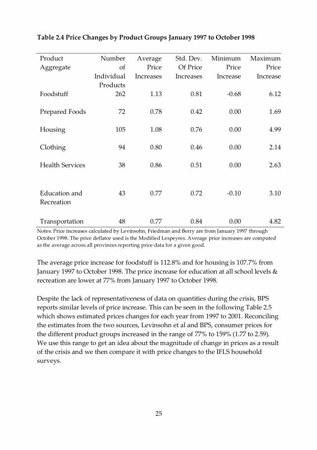
2.4 Price Changes by Product Groups January 1997 to October 1998.................................. 25

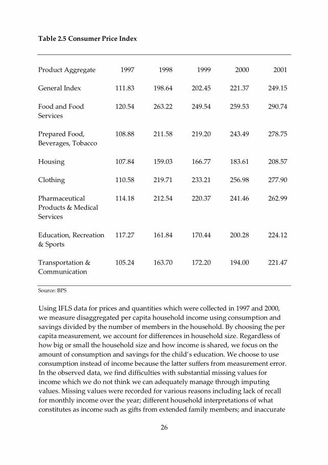
2.5 Consumer Price Index ...................................................................................................... 26

2.6 Price Indices ...................................................................................................................... 29

2.7 Household Income Per Capita ......................................................................................... 30

2.8 Household Spending on Education ................................................................................. 32

2.9 Expenditure Type as Share of Total Educational Expenditures .................................... 34

2.10 Households Reporting Zero Spent by Educational Expenditure Type........................ 35

2.11 Children Attending Different School Types .................................................................. 40

2.12 Characteristics of Children who Transition and Do Not Transition to Junior High ... 43

3.1 Indonesia Total Installed Capacity and Electricity Consumption 1997 - 2000 .............. 53

3.2 Distribution of Final Energy Use by Sector in Indonesia............................................... 54

3.3 MONE / MORA School Census Data – School Conditions Checklist ............................ 55

3.4 Measures of Association between Educational Performance, Electricity in School and

Electricity at Home in 1997 .................................................................................................... 61

3.5 Measures of Association between Educational Performance, Electricity in School and

Electricity at Home in 2000 .................................................................................................... 62

3.6 Measures of Association between Educational Performance, Electricity in School and

Electricity at Home for 1997 / 2000 ........................................................................................ 63

3.7 Descriptive Statistics......................................................................................................... 65

3.8 Electricity Availability and Educational Performance.................................................... 69

3.9 Electricity Availability, Use and Educational Performance ........................................... 73

4.1 Working Status of Children by Urban / Rural and Gender ........................................... 85

4.2 Children Working and Different Sources of Skill Formation ........................................ 95

4.3 Children Working outside the Household and Different Sources of Skill Formation . 95

4.4 Children Working in the Household and Different Sources of Skill Formation ........... 96

4.5 Characteristics of Children Working outside the Household ....................................... 97

4.6 Characteristics of Children Working in the Household ...............................................100

4.7 Household Income, Joint Work Outside-Schooling and Fulltime Schooling ..............103

4.8 Household Income, Joint Work Outside-Schooling and Joint Work in Household-

Schooling ..............................................................................................................................105

4.9 Household Income and Hours Worked by Child outside the Household while

Attending School .................................................................................................................108

5.1 Descriptive Statistics .......................................................................................................125

5.2 OLS & IV-2SLS Complementarity of Financial Investments in Junior High ...............131

5.3 OLS & IV-2SLS Complementarity of Financial Investments in Junior High ...............133

5.4 OLS & IV-2SLS Complementarity of Time Investments in Junior High ......................136

5.5 OLS & IV-2SLS Complementarity of Time Investments in Junior High .......................138

1

1. Introduction

2

1.1 Aim

Education is considered to be very important for economic growth. But family

investments in education are much lower in developing countries compared to

developed countries. This leads to the question whether families in developing

countries are less inclined to invest and whether the market rates of return are very

low; or that there are actually constraints to investment. Potential constraints are

basic facilities for schooling and low incomes. These constraints might not only

affect whether or not investments are made, but might also affect the extent and

quality of investments made. Spending a full day in school with limited basic

facilities might be less productive than going to school part of the day and rushing

home to help in the family enterprise and learn the trade. Families in developing

countries tend to face such constraints or “stumbling blocks” due to a multitude of

factors and unexpected events which might result in sub-optimal human capital

investments. In this dissertation we study two main constraints faced in the

Indonesian developing country context: resource constraints in basic facilities – we

use the access to and use of electricity for learning; and monetary constraints as

captured by family income.

The aim of this dissertation is to investigate the effects of inadequate basic facilities

on learning; and the effects of low income on educational investment. We consider

how these resource and income constraints affect the different dimensions of school

quality and educational outcomes. This investigation is carried out using data for

Indonesia over the period 1997 – 2000. To carry out this empirical analysis, we

adopt theoretical models of human capital from Becker (1964, 1993 updated), and

Cunha and Heckman (2007) and apply them within the context of Indonesian

children’s primary school and junior high education. The dataset that we use

throughout this dissertation is the RAND Corporation Indonesian Family Life

Surveys (IFLS) Wave 2 from 1997 and Wave 3 from 2000. Because of this dataset

that captures family strategic behavior in education, we are able to determine a

non-income resource constraint and income constraint for the following reasons.

First, as Indonesia is a large country there is sufficient geographic variation in

infrastructure to study the constraint of electricity access and use on schooling.

Parental investments in education differ in Indonesia because of huge variations in

regional development across the country with an estimated population of 237

million, land mass of 1.3 million km2 and over 13,000 islands. The main Java and

Bali islands have more advanced levels of economic development, more waged

labor opportunities and more schooling choice1. This is as opposed to the Outer

Islands that consist more of subsistence economies, agricultural economies and

1 Center for Studies in Higher Education, University of California at Berkeley 1991

3

have lower levels of economic development. In terms of electricity infrastructure,

Java and Bali have 77% of total capacity and the Outer Islands have the remaining

23%. Also because the Outer Islands are located further away from the central

government in Java and more difficult to access geographically there are fewer

quality schools available. Second, Indonesia faced the Asian Financial Crisis (AFC)

in end 1997 that lowered family incomes exogenously which provides us with an

instrument for income to study the effects of family income on child labor and

educational investments. Over the period of 1998 and 1999, the reduction in

household incomes produced a variety of observable behavioral responses towards

investment in education which makes this period ripe for a natural experiment2.

The differences observed in family strategic behavior provide us with the

opportunity to investigate various behavioral dimensions towards education.

In Indonesia investment in education is a goal shared by the family and the state.

This is highlighted in the opening chapter of the 1945 Republic of Indonesia

Constitution which explicitly states that one major goal of the state is to ensure the

intellectual development of all citizens of the country. While there is no

compulsory schooling age, the family and the state attempt to invest in at least 9

years of basic education for children aged 6 - 15. However, families face direct costs

and opportunity costs for schooling. Hence having 9 years of schooling is

considered an educational achievement in the country where only in recent

memory, achieving full adult literacy was still a long overdue goal. With economic

growth in Indonesia, there has been the expansion of schooling attainment. In the

country’s thirty year growth trajectory 1967 - 1997 universal primary education was

on target to be achieved and to be followed by an increase in junior high. By 1997, a

peak of 80% of all school children who enrolled in school had attained 9 years of

education in primary school and junior high while the remaining 20% dropped out.

But after 1997 coinciding with the crisis, the percentage of children who attained 9

years of schooling fell to 75% and the trend has since deteriorated to 52.6% in 2001;

and this negative trend continues to hold after 20013.

2 Why is the financial crisis as a natural experiment an opportunity? First and foremost this is an

opportunity because it is not possible to create a randomized controlled trial using the whole Indonesian

population as treatment and control subjects. Second and lyrically, we cite the econometrics forefather

Trygve Haavelmo (1944) and his thoughts on natural experiments: “the stream of experiments that

Nature is steadily turning out from her own enormous laboratory, and which we merely watch as

passive observers. The aim of the theory (behind experimental designs) is to become master of the

happenings of real life.” Also more recently, Jared Diamond and James A. Robinson (2010) write about

“Natural Experiments of History” on the basis that some central questions in the natural and social

sciences can’t be answered by controlled laboratory experiments. One has to then devise other methods

of observing, devising and explaining the world. 3 Indonesia Ministry of National Education (MONE)

4

In the literature on education in developing countries, children tend not to receive a

full basic education mainly because of credit constraints where there is limited

scope for borrowing in order to invest in education (Galor and Moav, 1999; Foster

and Rosenzweig, 2000; Glewwe and Jacoby, 2000, Glewwe and Kremer, 2005). Most

of the financial investment in education therefore has to be funded by the family. In

Indonesia, up to 60% of total financing for education is funded by the family

(World Bank, 2007). Hence how the family makes it decisions for educational

investment is a crucial issue. This is as argued by Rosen (1989) and Glewwe and

Kremer (2005) where it is not just credit constraints but the nature of family

decision making as well that will provide a better understanding of how much

education children attain. The parental decision to finance more or fewer years of

schooling is influenced by the private rate of return to additional years of schooling

(Psacharopoulos, 1994 and Psacharopoulos and Patrinos, 2004). Parental decision

making is also influenced by the value added to cognitive skills from each

additional year of schooling (Harbison and Hanushek, 1992; Hanushek and

Wößmann, 2010). Also Harbison and Hanushek (1992) find that some parents in

developing countries are predisposed to education for their children simply when a

minimum standard of school resources are available i.e. the school has a permanent

physical structure as opposed to temporary arrangements. Because of the various

considerations that parents make when deciding to finance their children’s

education, it is no longer simply a question of having the financing to attend or not

to attend school. The calculus of decision making involves how much schooling to

attain, whether the school has sufficient resources, the quality of knowledge and

skills accumulated; and parents’ perceived private and social returns to education.

While studying the empirics of family income and human capital is interesting in

its own right, these dissertation findings provide new information for development

policymaking. National development planners in Indonesia and foreign aid donors

have put much focus on improving school resources for the formal education

system in order to achieve the country’s educational goals. The government builds

more schools for formal education, buys more computers, trains more teachers and

tinkers more with the academic curriculum. To complement this would be more

understanding of the nature of decision making by parents for their children’s

future – the environment in which they live and not just the school specific

environment for education, what they do each day, what difficulties they face each

day and the multitudes of decisions they take for investing in their children. The

findings in this dissertation provide some policy implications concerning how

these two constraints affect educational investment decision making from a

monetary and non-monetary perspective. These findings may perhaps be of useful

application to the geographically large and socio-economically diverse developing

countries of Brazil, China and India that are faced with varying school quality.

5

1.2 Human Capital Accumulation, School Resources,

Outputs & Outcomes To carry out our empirical investigation, we review human capital concepts and

introduce the ways in which we measure them as educational inputs, outputs and

outcomes. These concepts and measures are derived from Becker (1964, 1993

updated), Hanushek (2006), Hanushek and Wößmann (2008), Cunha, Heckman,

Lochner and Masterov (2006) and Cunha and Heckman (2007).

1.2.1 Human Capital Accumulation

Following Becker, we view human capital as a stock of knowledge or skills that are

directly useful in the production process. Becker also recognizes that knowledge

and skills can be gained not just from school but from various sources and these

sources are elaborated upon by the Coleman Report (1966). To capture the

knowledge and skills from each additional year of schooling as a part of a total

stock, we mainly use the Indonesian national standardized achievement test scores

EBTANAS at the end of a given school level. Together with the initial endowments

when the child is born which are unobserved, additional knowledge and skills

increase the size of this stock. But the marginal benefits decline as additional capital

is accumulated. This can be due to memory capacity, a requisite skill or ability that

is not present to build new skills, etc. The implication is that eventually over the

child’s life cycle, diminishing returns set in from producing additional capital (Ben-

Porath, 1967). It becomes more costly to accumulate more human capital when the

child is older; and at a later school level compared to an earlier school level. To

then maximize the returns to human capital, parents should increase the

productivity of early knowledge and skills accumulated by making further

investments when the child is older. This can be related to complementary

investments in human capital (Cunha, Heckman, Lochner and Masterov, 2006).

1.2.2 School Resources

To build a stock of knowledge and skills requires school resources or educational

inputs for use in the educational production process. Using the structure of the

Indonesia national education system and educational policy, we determine the

characteristics of these school resources. Also we study how these school resources

relate to school quality and the implications for how much or how little family

income can do to acquire school quality (Glewwe, 2002 and Hanushek, 2009). Even

if a family in a developing country has high income, they may reside in an area

geographically that has limited schooling choice. This family for unobserved

reasons may also have low mobility i.e. there might be a low inclination to migrate

6

for education. As such they may be able to do very little using income to improve

the quality of schooling inputs available in their residential area.

The school resources that we investigate in Indonesia are school facilities

particularly electricity, teacher qualifications, the curriculum taught, the

availability of textbooks and the mode of learning. Closely related to school quality,

we study how these schooling inputs differ for children in the high quality formal

education system and children in low quality alternative education (non-formal

and informal schools).

1.2.3 Outputs

As the Indonesian national educational system recognizes but differentiates

between formal education and alternative education (non-formal and informal

schools), we use different measures of school attendance for formal education and

alternative education as educational outputs. For the formal education system, we

use each year of school enrollment as an output measure. For alternative education,

we use registration in a non-formal or informal school as a mode of learning as an

output measure. For both formal education and alternative education, available

data enables us to include as an output measure, time allocated to the learning

process over the period of a day and a week. This output measure of time

allocation includes the dimensions of time for classroom instruction and studying

in the evening after school. Time allocation for schooling also enables us to analyze

the relative value of a child’s time between schooling and work.

1.2.4 Outcomes

While many empirical studies define educational outcomes in terms of the number

of years of schooling enrollment, we take a different approach by using the

measure for transition between school levels as represented by the EBTANAS

standardized achievement tests. The full set of tests for EBTANAS consists of the

national language Bahasa Indonesia, Mathematics, Science, Social Studies and

Religious Studies. By passing EBTANAS at the end of the primary school level, the

child is qualified to transition to the junior high level.

Only children in the mainstream, formal education system are entitled to directly

sit for EBTANAS at the end of a school level. Children who are in alternative

schools such as non-formal school for child workers and informal school for

children who are home schooled or are child apprentices are entitled to sit for these

tests if they switch to the formal system and complete the full cycle of a school

level.

7

Transition from one school level to the next is both an output and outcome of the

educational process because it measures the number of schooling years attained

and the level of knowledge and skills attained. This measurement indicator is

important from both a technical and policy perspective. From a technical

perspective, a child’s labor market outcomes in adulthood can be traced back to the

number of schooling levels completed and qualifications attained for each level. In

Indonesia’s structured and hierarchical education system, the first transition is

from primary school to junior high. The second transition is from junior high to

senior high. The third transition is from senior high to tertiary education. Each

additional schooling year completed does not matter but each additional schooling

level completed matters because of the qualification received at the end of a level.

From a policy perspective, transition rates matter for the achievement of national

educational policy and the Indonesia UN Millennium Development Goal #2 of 9

years of universal basic education.

We do not use enrollment as an outcome measure in any of the chapters for various

reasons. Based on UNESCO technical guidelines, enrollment is recorded as

registration on the first day of the school year. Or it is recorded during a census. As

such this measurement indicator does not accurately capture school attendance

flows throughout the school year. As pointed out by Krueger and Lindahl (2001),

enrollment rates are then a flawed measure for human capital. Most importantly,

Hanushek and Wößmann (2008) argue that using years of schooling enrollment as

an education measure implicitly assumes that a year of schooling delivers the same

increase in knowledge and skills regardless of the education system i.e. the

difference between formal education and alternative education in Indonesia. The

school enrollment measure also assumes that formal education is the primary

source of education and variations in the quality of non-school factors affecting

learning such as where children are raised and their daily learning environment i.e.

family enterprise and lack of electricity have a negligible effect on human capital

outcomes.

1.3 Outline This dissertation consists of five chapters4. Chapter 2 provides the departure point

for the dissertation with a detailed description of the Indonesian national education

system and an overview of the AFC context. This is then followed by a descriptive

analysis of changes to Indonesian family educational investment behavior. The

changes are documented by comparing families in 1997 and families in 2000 that

4 The five chapters have been revised from four individual papers.

8

have similar characteristics. Also we justify using the crisis as a valid instrument

for income. We show that the AFC is relevant because it is correlated with income

and it is plausibly exogenous because it is not directly correlated with educational

investments but through its correlation with income. As Chapter 2 maps out the

role of the family in making educational investment decisions given available

income and time, schooling prices and the institutional environment, we are able to

then determine the two constraints for investment. We proceed to study the

resource constraint in Chapter 3 and the income constraint in Chapters 4 and 5. For

Chapters 4 and 5, we specifically use the AFC as an instrument for household

income. From these chapters, we determine that there are two constraints to the

amount and quality of educational investment: i) resources for basic facilities -

electricity, ii) low family income. The resource constraint is a non-income constraint

as it is not easily influenced by family income and together with the income

constraint, affect the quality of schooling inputs used for education, the number of

schooling years attained, the completion of school levels and educational

achievement. Chapter 6 provides a summary of this dissertation and implications

for policy. We will now elaborate on the structure of the chapters, methods used

and the line of thought.

1.3.1 Family Educational Spending when Income Falls

In Chapter 2, we describe the national education system and the environment when

the financial crisis occurred from end of 1997 - 2000. We then map out the role of

the family in making educational investment decisions for children aged 6 – 15.

This is given available income and time, real schooling prices and the institutional

environment. We document changes to family decision making by comparing

families in 1997 with families in 2000 that have similar characteristics. We carry out

a review of the extensive literature that was written to document the volatile

changes to prices and we isolate the price of schooling, incomes, consumption and

schooling behavior. We show that parents respond to an income reduction by

compromising on the quantity and quality of education that their children attain.

We then report on the various strategies families in different geographical areas

took for their children’s education. The documentation of these educational

investment responses to the financial crisis then justifies the use of the crisis as a

valid instrument for income. The crisis is used as an instrument in Chapters 4 and

5.

1.3.2 Electricity Access, Use and Children’s Educational

Performance

In Chapter 3, we study whether there is a correlation between the availability of

electricity in schools and households and educational performance at age 12. The

9

potential relationship between the two main variables of interest is via the use of

electricity in school and at home. We use pooled data from 1997 and 2000 which

consist of regional variation in electricity availability. We find that there exists a

positive correlational relationship between access to electricity and educational

performance. We find this result in both developed and underdeveloped, left

behind regions of the country. However children in underdeveloped, below-the-

poverty-line areas have lower test score performance than children in developed

areas. Using access to electricity, this chapter shows that the family can be

confronted with overall resource constraints in basic facilities for schooling. When

the educational performance of disadvantaged 12 year old children in

underdeveloped areas is found to be lagging behind, resource constraints may

prevent the children from progressing on to junior high.

1.3.3 Family Income, Simultaneous Work-Schooling and

Human Capital

In Chapter 4, we investigate the relationship between family income and child

labor in terms of the behavior of children who allocate time to work and attending

school simultaneously. This chapter documents how child workers can choose to

attend formal school, non-formal school or informal school. Using a natural

experiment with IV estimation, we find that a fall in income results in a shift away

from full time schooling to joint work-schooling. Within the joint work-schooling

decision, an income decrease is also found to increase the propensity to shift more

away from schooling and shift more towards work. Unexpectedly family income is

not the main constraint that prevents full time schooling. What drives the joint

work-schooling decision is the age of the child. After age 12, children are inclined

to work more and attend school less which increases the risk of failing to complete

a full course of 9 years of basic education.

1.3.4 Dynamic Complementarity of Investment in Education

In Chapter 5, we study the role of family income on financial and time investments

in education. We apply the Cunha and Heckman (2007) theoretical formulation for

the technology of skill formation. Using repeated cross sections from 1997 and

2000, we find that about 80% of the cross-sectional link between income and

educational expenditures is caused by differences in income. The remaining 20% is

related to unobserved income related parental characteristics. But lower

educational expenditures due to less income are highly compensated by time

investments. This strongly implies that income related parental characteristics as

well as unobserved child characteristics explain a substantial part of these

compensating time investments. But this is only for higher ability children who

10

have selected to complete primary school and transition to junior high. Also the

reduction in educational expenditures is much lower for children who have already

attained a few years of junior high education compared to children who have just

begun junior high. This then suggests that optimal education investment does

include accounting for the loss in returns from previous investments on the stock of

human capital that has been accumulated. Put another way, parents do face a loss

aversion where sunk costs do matter. Taken together these results reveal that

income constraints do restrict parents in their educational expenditures, that they

are concerned with future returns; and that especially parents with favorable

characteristics compensate reductions in educational expenditures by letting their

children spend more time in school.

1.3.5 Main Findings and Implications

The main findings of the dissertation are reviewed in Chapter 6 and we discuss the

implications of the role of the family in increasing human capital in developing

countries. By providing insight into the disadvantaged family and the resource

constraints and income constraints they are confronted with, we will be able to

better determine how to increase a child’s schooling attainment and educational

achievement

11

2. Family Educational Spending when Income

Falls

12

2.1 Introduction

In this chapter we describe educational spending in Indonesia and how it was

affected by the Asian Financial Crisis (AFC). The AFC reduced economic growth,

increased unemployment, substantially increased inflation and severely reduced

household purchasing power. Because of reduced income, households made

adjustments to daily expenditures, savings and budget allocations for their

children’s education.

Our aims are to document how households spent on education before the crisis;

how spending and schooling participation patterns changed in response to an

income reduction; and how these patterns are influenced by where the household

resides geographically in the Indonesian archipelago. Available data provides us

with the opportunity to examine not just whether parents continued to spend on

education and send their children to school when income fell but also the extent to

which schooling quality changed, as well as how schooling participation was

affected by the incidence of child labor.

We trace the effects of extreme increases in the general prices of goods and services

on household consumption and savings down to spending decisions for the child’s

education. We document these responses for children in primary school and junior

high. Regardless of extremely high levels of inflation and volatility in currency

exchange rates, we find that the children still managed to receive an education.

However the fall in household income reduced the quality of schooling purchased.

We document an increase in the number of children in schools that have lower

quality schooling inputs. We also find evidence that educational outcomes

deteriorated. There is evidence too that a smaller proportion of children

transitioned from the primary school level to the junior high level.

Sparrow (2006) who studied Indonesia state intervention during the financial crisis

found that targeted subsidies maintained enrollment flows; and it seemed to

relieve pressure on household spending in education. We expand on Sparrow’s

work on enrollment flows and study the quality of schooling inputs and outcomes

at the time. We use measures that encompass different schooling inputs which

includes school type (formal education and alternative education) and school

provision type (publicly funded and managed and privately funded and managed).

Our measures of educational outcomes are the EBTANAS national standardized

achievement test scores and transition rates. The rest of the chapter is organized in

the following way. Section 2.2 provides a general overview of the country. Section

13

2.3 provides the context in terms of the AFC occurring at the time and a detailed

description of the national educational system. In section 2.4 we describe the data

and where we carry out a pair-wise matching of households and schools in the

same community to enable comparison and use separate price deflators for

education and non-education goods. In section 2.5 we map out the changes to the

price of goods and services, household income and educational spending. Given

these changes we analyze adjustments to the different parental spending strategies

for their children. Section 2.6 covers the conclusions made from the documented

changes and makes linkages to Chapter 3 which investigates how spending is

influenced by where the household resides in the Indonesian archipelago.

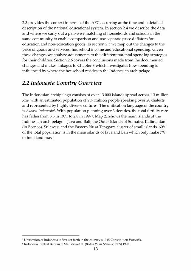
2.2 Indonesia Country Overview

The Indonesian archipelago consists of over 13,000 islands spread across 1.3 million

km2 with an estimated population of 237 million people speaking over 20 dialects

and represented by highly diverse cultures. The unification language of the country

is Bahasa Indonesia5. With population planning over 3 decades, the total fertility rate

has fallen from 5.6 in 1971 to 2.8 in 19976. Map 2.1shows the main islands of the

Indonesian archipelago – Java and Bali; the Outer Islands of Sumatra, Kalimantan

(in Borneo), Sulawesi and the Eastern Nusa Tenggara cluster of small islands. 60%

of the total population is in the main islands of Java and Bali which only make 7%

of total land mass.

5 Unification of Indonesia is first set forth in the country’s 1945 Constitution Pancasila. 6 Indonesia Central Bureau of Statistics et al. (Badan Pusat Statistik, BPS) 1998

14

Figure 2.1 Map of the Indonesian Archipelago

2.3 Institutional Context – Asian Financial Crisis and

National Educational System

2.3.1 Asian Financial Crisis

The AFC occurred at the end of 1997 with effects in the financial markets felt until

the beginning of 2000. It had interrupted a thirty year period of rapid growth in

East and South East Asia. In Indonesia, real per capita GDP rose four-fold between

1965 and 1995 with an annual growth rate averaging 4.5% until the 1990s when it

rose to almost 5.5% (World Bank, 1997). The poverty headcount rate declined from

over 40% in 1976 to just under 18% by 1996. The country’s domestic savings level

reached 30% prior to 1997. Primary school enrollment rates rose from 75% in 1970

to universal enrollment by 1995 and secondary enrollment rates from 13% to 55%

over the same period (World Bank, 1997).

In April 1997, the financial crisis began to be felt in the Southeast Asian region,

although the major impact did not hit Indonesia until December 1997 and January

1998. With reference to the following Table 2.1, which consists of macroeconomic

data, GDP growth fell from 4.70% in 1997 to -13.13% in 1998 and then rising to

0.79% in 1999 before reaching pre-crisis growth rates in 2000. Annual inflation rates

increased from 6.23% in 1997 to 58.39% in 1998 and then improving to 20.49% in

1999 before resuming a considerably lower rate of 3.72% in 2000. The trend for

15

gross domestic savings as a percentage of GDP presented a pattern of offsetting the

massive spike in inflation rates. While savings were at a high of 31.48% in 1997,

there was a decreasing trend from 1998 to 2000.

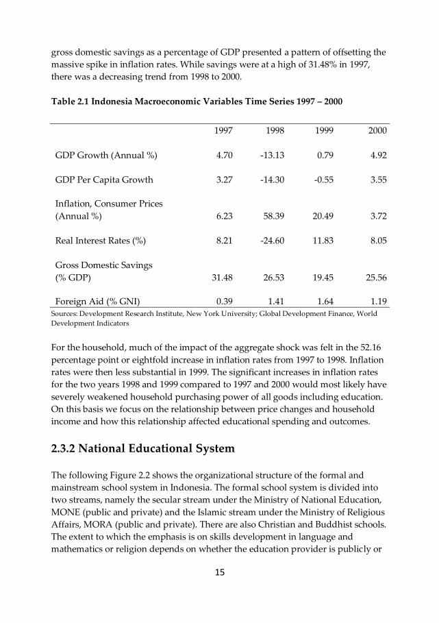
Table 2.1 Indonesia Macroeconomic Variables Time Series 1997 – 2000

1997 1998 1999 2000

GDP Growth (Annual %) 4.70 -13.13 0.79 4.92

GDP Per Capita Growth 3.27 -14.30 -0.55 3.55

Inflation, Consumer Prices

(Annual %) 6.23 58.39 20.49 3.72

Real Interest Rates (%) 8.21 -24.60 11.83 8.05

Gross Domestic Savings

(% GDP) 31.48 26.53 19.45 25.56

Foreign Aid (% GNI) 0.39 1.41 1.64 1.19 Sources: Development Research Institute, New York University; Global Development Finance, World

Development Indicators

For the household, much of the impact of the aggregate shock was felt in the 52.16

percentage point or eightfold increase in inflation rates from 1997 to 1998. Inflation

rates were then less substantial in 1999. The significant increases in inflation rates

for the two years 1998 and 1999 compared to 1997 and 2000 would most likely have

severely weakened household purchasing power of all goods including education.

On this basis we focus on the relationship between price changes and household

income and how this relationship affected educational spending and outcomes.

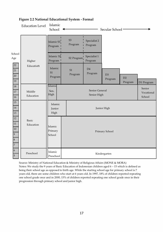
2.3.2 National Educational System

The following Figure 2.2 shows the organizational structure of the formal and

mainstream school system in Indonesia. The formal school system is divided into

two streams, namely the secular stream under the Ministry of National Education,

MONE (public and private) and the Islamic stream under the Ministry of Religious

Affairs, MORA (public and private). There are also Christian and Buddhist schools.

The extent to which the emphasis is on skills development in language and

mathematics or religion depends on whether the education provider is publicly or

16

privately funded and whether the education provider is regulated by MONE or

MORA.

Contrary to practices in many other countries, the public sector provides higher

quality education than the private sector (Lanjouw, Pradhan, Saadah, Sayed and

Sparrow, 2001; Newhouse and Beegle, 2005). The differences in quality between

public and private schools are in terms of schooling inputs (Newhouse and Beegle,

2005). Based on their studies of junior high schools, in public schools textbooks are

more easily available and teachers have higher educational qualifications

compared to private schools.

Since the end of the Suharto regime and the introduction of regional autonomy

laws, there is an increasing trend of schooling provision by religious associations

and non-governmental organizations. These private providers of education retain

the option to adjust the curriculum to a greater extent to meet local indigenous

needs. These include a curriculum covering local agricultural farming methods,

environmental education and local culture - traditional arts and languages /

dialects.

17

Figure 2.2 National Educational System - Formal

Source: Ministry of National Education & Ministry of Religious Affairs (MONE & MORA)

Notes: We study the 9 years of Basic Education of Indonesian children aged 6 – 15 which is defined as

being their school age as opposed to birth age. While the starting school age for primary school is 7

years old, there are some children who start at 6 years old. In 1997, 18% of children reported repeating

one school grade once and in 2000, 15% of children reported repeating one school grade once in their

progression through primary school and junior high.

Preschool

Basic

Education

Middle

Education

Highe

r Educatio

n

Higher

Education 22

21

20

19

18

17

16

15

14

13

12

11

10

9

8

7

6

5

School

Age

Kindergarte Islamic

Preschool

Islamic

Primary

School Primary Junior

High

Schoolchool

Islamic

Junior

High

Junior High

Islamic

Sen. High

Senior General

Senior High

Islamic S1

Program

S1 Program

D4

Program D3

Program D2

Program D1 Program

Islamic S2 Program

S2 Program Specialist 1

Program

Islamic S3 Program

S3

Program

Specialist 2 Program

Senior

Vocational

School

Kindergarten

Education Level Islamic

School Secular School

Primary School

18

Figure 2.3 shows the expanded organizational structure of the education system

that incorporates both formal schooling and alternative schooling. In this figure,

formal schooling is represented by in-school education and non-formal and

informal schooling are represented by out-of-school education. For disadvantaged

children e.g. child workers who have fewer fulltime educational opportunities the

education system provides two alternatives to the formal, mainstream system – the

non-formal school and informal school / education by the family.

Figure 2.3 National Educational System – Formal and Informal

School

Age

In-School Education Out-of-School Education

Formal Non Formal Informal

>22 Higher Education / Religious Higher Education Post

Grad

Education by

the Family

19 - 22 Higher Education / Religious Education Grad /

Diploma

16 - 18 Senior High Apprenticeship

Packet C

General Vocational

General Religious

Education

General Religious

Education

13 - 15 Junior High Junior High

Equivalent

Packet B

General

Religious Education

6 or 7 -

12

Primary School Primary School

Equivalent

Packet A

General

Religious Education

The non-formal school system consists of equivalency educational programs,

Packet A (equivalent to primary school) and Packet B (equivalent to junior high);

and vocational training programs provided by non-governmental organizations.

Private religious schools funded from charitable contributions and not

administered by MORA also provide non-formal education. Children who choose

the equivalency educational programs have the flexibility of customizing time for

learning around time for working. For example, if a child has to work on the farm

in the morning and late afternoon, s / he can attend classes with a tutor in the early

afternoon.

19

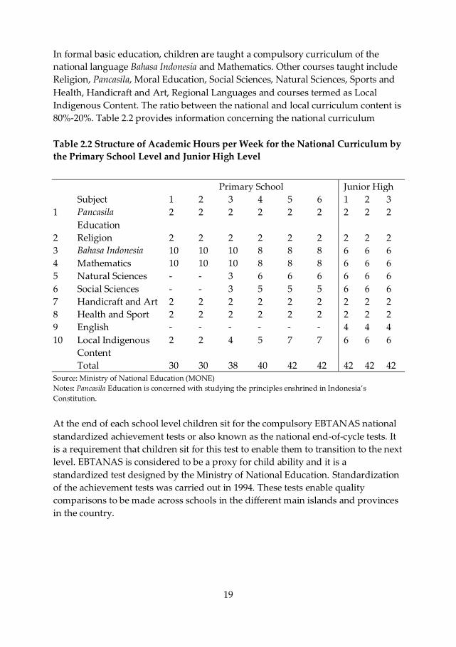
In formal basic education, children are taught a compulsory curriculum of the

national language Bahasa Indonesia and Mathematics. Other courses taught include

Religion, Pancasila, Moral Education, Social Sciences, Natural Sciences, Sports and

Health, Handicraft and Art, Regional Languages and courses termed as Local

Indigenous Content. The ratio between the national and local curriculum content is

80%-20%. Table 2.2 provides information concerning the national curriculum

Table 2.2 Structure of Academic Hours per Week for the National Curriculum by

the Primary School Level and Junior High Level

Primary School Junior High

Subject 1 2 3 4 5 6 1 2 3

1 Pancasila

Education

2 2 2 2 2 2 2 2 2

2 Religion 2 2 2 2 2 2 2 2 2

3 Bahasa Indonesia 10 10 10 8 8 8 6 6 6

4 Mathematics 10 10 10 8 8 8 6 6 6

5 Natural Sciences - - 3 6 6 6 6 6 6

6 Social Sciences - - 3 5 5 5 6 6 6

7 Handicraft and Art 2 2 2 2 2 2 2 2 2

8 Health and Sport 2 2 2 2 2 2 2 2 2

9 English - - - - - - 4 4 4

10 Local Indigenous

Content

2 2 4 5 7 7 6 6 6

Total 30 30 38 40 42 42 42 42 42 Source: Ministry of National Education (MONE)

Notes: Pancasila Education is concerned with studying the principles enshrined in Indonesia’s

Constitution.

At the end of each school level children sit for the compulsory EBTANAS national

standardized achievement tests or also known as the national end-of-cycle tests. It

is a requirement that children sit for this test to enable them to transition to the next

level. EBTANAS is considered to be a proxy for child ability and it is a

standardized test designed by the Ministry of National Education. Standardization

of the achievement tests was carried out in 1994. These tests enable quality

comparisons to be made across schools in the different main islands and provinces

in the country.

20

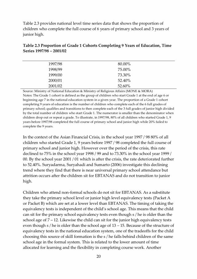
Table 2.3 provides national level time series data that shows the proportion of

children who complete the full course of 6 years of primary school and 3 years of

junior high.

Table 2.3 Proportion of Grade 1 Cohorts Completing 9 Years of Education, Time

Series 1997/98 – 2001/02

1997/98 80.00%

1998/99 75.00%

1999/00 73.30%

2000/01 52.40%

2001/02 52.60% Source: Ministry of National Education & Ministry of Religious Affairs (MONE & MORA)

Notes: The Grade 1 cohort is defined as the group of children who start Grade 1 at the end of age 6 or

beginning age 7 in the national education system in a given year. The proportion of a Grade 1 cohort

completing 9 years of education is the number of children who complete each of the 6 full grades of

primary school; qualifies and transitions to then complete each of the 3 full grades of junior high divided

by the total number of children who start Grade 1. The numerator is smaller than the denominator when

children drop out or repeat a grade. To illustrate, in 1997/98, 80% of all children who started Grade 1, 9

years before 1997/98 completed the full course of primary school and junior high while 20% failed to

complete the 9 years.

In the context of the Asian Financial Crisis, in the school year 1997 / 98 80% of all

children who started Grade 1, 9 years before 1997 / 98 completed the full course of

primary school and junior high. However over the period of the crisis, this rate

declined to 75% in the school year 1998 / 99 and to 73.30% in the school year 1999 /

00. By the school year 2001 / 01 which is after the crisis, the rate deteriorated further

to 52.40%. Suryadarma, Suryahadi and Sumarto (2006) investigate this declining

trend where they find that there is near universal primary school attendance but

attrition occurs after the children sit for EBTANAS and do not transition to junior

high.

Children who attend non-formal schools do not sit for EBTANAS. As a substitute

they take the primary school level or junior high level equivalency tests (Packet A

or Packet B) which are set at a lower level than EBTANAS. The timing of taking the

equivalency tests is independent of the child’s school age. This means that the child

can sit for the primary school equivalency tests even though s / he is older than the

school age of 7 – 12. Likewise the child can sit for the junior high equivalency tests

even though s / he is older than the school age of 13 – 15. Because of the structure of

equivalency tests in the national education system, one of the tradeoffs for the child

choosing this source of skill formation is the s / he falls behind children of the same

school age in the formal system. This is related to the lower amount of time

allocated for learning and the flexibility in completing course work. Another

21

tradeoff is that the child forgoes the EBTANAS credential for entering the labor

market. This is unless the child enters the formal system and starts the education

process from the beginning at grade 1.

The informal school is a source of skill formation that is derived from education or

skill development in the home. This includes apprenticeships, learning-on-the-job

or home production / domestic work. Children from informal schools also do not

sit for EBTANAS. However like children in non-formal school, they sit for the

equivalency tests. Children who make this schooling choice experience different

tradeoffs from children in non-formal schools. On the one hand, these children are

developing productive skills within the family business or trade and these skills

may also have private returns in the economy. The acquisition of such skills is

consistent with Becker’s theory of human capital accumulation. On the other hand

the tradeoff is that these skills may be valued in the economy as unskilled or low

skilled wages in comparison to the premium that skilled wages receive in the labor

market. However the wage premium for skilled labor in the economy is dependent

on the characteristics and relationships of the formal and informal sectors in

Indonesia. Another tradeoff of skill acquisition from the informal school is that if

parents perceive a higher value from the children working and learning within the

family business, their children will spend more time in the household and be less

inclined to allocate time for attending school.

For this chapter we focus on basic education consisting of primary school, ages 6 –

12; junior high school, ages 13 – 15 and the alternative schooling equivalent for

these school ages. But we do not provide an in-depth analysis of alternative

schooling in this chapter. We will do this in Chapter 4 when we examine the

incidence of simultaneous work-schooling behavior.

The education system is financed in broad terms by four sources: 1) funds from

general government revenue 2) government revenues earmarked for education 3)

tuition and other fees 4) voluntary contributions. In terms of the first two sources,

this refers to central and regional government where by constitutional law, the

central government should fund 20% of the total funding required each year.

Revenues earmarked for education include foreign aid assistance. The third source

of funding comes from the household and this varies based on the number of

children being sent to school at the same time. The fourth source includes gifts

from individuals, communities, charitable and religious bodies, domestic or

foreign, whether in cash, kind or services; endowments, commercial or private

loans; and the schools’ own efforts to raise funds (Daroesman, 1971). Based on

World Bank records (2007), the general split of funding sources for the education

system is 1) central government, 20% 2) regional / local government, 20% and 3)

other sources including parents’ contributions, 60%.

22

In end 1998, during the period of the financial crisis, MONE / MORA introduced a

scholarship and block grant program for disadvantaged children in primary and

junior high schools. This subsidy program was aimed at maintaining enrollments

and maintaining the quality of basic education at pre-crisis levels. The scholarships

were provided to the schools who then selected the children who would receive the

scholarships. Groups of children identified by MONE / MORA as having the

highest likelihood of dropping out of school because of the crisis were students

from households with reduced incomes; primary school leavers who were not

likely to transition to junior high; junior high school leavers who were not likely to

transition to senior high; and girl teenagers who did not complete primary and

junior high schooling. These groups of children were targeted by MONE / MORA

as being in the poorest schools in a district and this was defined as schools in low

income districts; schools that required parents to make higher than average

monthly scheduled payments to cover operating costs; and schools that served

students who live in government designated left behind villages (INPRES Desa

Tertinggal, IDT). However it was acknowledged by MONE/MORA that it did not

have full information concerning school conditions and the socio-economic

background of the disadvantaged communities. This is because such information is

mostly unavailable at the aggregate district level.

Using this description of the Indonesian education system, we document

household spending behavior that includes the different groups of children defined

as being at risk of dropping out. Given the institutional context, educational

spending behavior entails credit constrained parents making decisions on whether

to finance their children’s education given upfront costs and delayed benefits and

the mechanics of how their children receive an education. Various schooling

participation strategies available to parents were - children could attend formal

schooling or alternative schooling – religious schooling, home schooling

apprenticeships, on-the-job training or a combination of methods. Within one

school day, children could spend half their time in school and the other half of the

time working with livestock, learning local animal husbandry.

2.4 Data

The dataset that is used is the RAND Corporation Indonesian Family Life Surveys

(IFLS). We use Waves 2 – 1997 and 3 – 2000. The sample size for Wave 2 is 10,356

individual observations and for Wave 3 it is 11,686 individual observations. Data

for Wave 2 was captured at the end of 1997 when the financial crisis was about to

occur and data for Wave 2 was captured at the end of the financial crisis in 2000.

We use data from Wave 2 concerned with retrospective economic and schooling

behavior covering the calendar year January – December 1997 and retrospective

23

behavior for the school year July 1996 – June 1997. Similarly we use data from

Wave 3 concerning retrospective economic and schooling behavior covering the

calendar year January – December 2000 and the school year July 1999 – June 2000.

IFLS consists of an additional Wave 2+ which was collected during the period of

the financial crisis but this data is not publicly available. So we assume that the

market source of price changes experienced by the household by its given location

in 1999 is the same in 2000.

We merge observed data on household income to observed data on educational

spending from separate IFLS books using an ID that matches the child aged 6 – 15

to the household7. Only biological parent-child relationships are considered. We

then proceed to match income and education spending data to schooling data from

another IFLS book. The schooling data that we have covers the schools available to

the children within each community. In the observed data, all children can reach

their school in not more than thirty minutes whether they go on foot or by using

different modes of transportation. In the data, we find that a child can report

attending more than one school in the community in a school year. This can be seen

by the presence of more than one school ID matched to each child. The school

types available are either MONE / MORA registered, publicly funded and

managed; MONE / MORA registered, privately funded and managed or non-

registered schools with alternative learning methods. Also the schooling data

covers information on whether the children benefitted from the national

educational scholarship and whether schools participated in the block grant

program for the school years 1999 and 2000. In the observed data, 4% of all children

received MONE / MORA scholarships for the school years 1999 and 2000.

Educational spending data is captured in IFLS as the annual amount of household

spending on education. In the observed data, educational expenditures consist of

one time payments in the school year and streams of repeated payments across the

school year. One time payments are the registration fee on the first day of the school

year, the fee for taking the exams at the end of the school grade, a set of textbooks

for the current school grade, writing supplies, uniform, sneakers and sports

equipment. Repeated payments within the school year consist of the monthly

scheduled parental contribution to the school’s operating costs, transportation to

and from school and private tuition outside of school hours. As described in Section

2.2.2 parental contributions for keeping the school running makes up a dominant

60% of total funding required.

As comparable income and education variables are available in Waves 2 and 3, we

carry out a pair-wise matching of children in 1997 and 2000 that have the same age

7 While the school age for starting primary school is 7, some children start primary school at age 6.

24

group, household and schooling characteristics. These characteristics include where

children reside and go to school in terms of island, province and urban-rural, school

type; whether they have repeated a grade in primary school or in junior high8, the

curriculum and by the school age of 12, the EBTANAS test score. Because of the

consumer price variation over the period, we can then compare changes to spending

strategies for children in the same age group progressing through the same

educational system. In the next section, we will use general prices, income and

education prices to document the changes.

2.5 Prices, Income and Education

2.5.1 Price Indices

In this sub-section, we describe the price deflators in use, why we choose certain

price deflators over others and the reasoning for the type of goods and services to

include or exclude from the computations.

As a departure point, we review the price and quantity data used by the Indonesia

Central Bureau of Statistics (BPS) to calculate consumer prices and to estimate

household purchasing power. BPS uses the Modified Lespeyres formula to

calculate real prices. The bureau collects price and quantity data at the national

level and provides information on household level consumption using the BPS

SUSENAS household surveys. But we are unable to use the BPS price and quantity

data for a more detailed analysis. This is because the BPS baseline quantities for

urban areas are from 1996 and for rural areas from 1993, both periods that are

before the financial crisis which are not representative of consumer prices during the

crisis; and both baseline quantities had not yet been revised at the time of the crisis.

To cover the period of prices before and during the financial crisis, we then

reference Levinsohn, Friedman and Berry (1999) who have done extensive work

measuring price changes and have the most available and reliable data. They use

the Modified Lespeyres price deflator and the aggregate level SUSENAS data and

their estimates capture 184 products and the price changes from January 1997

through October 1998. These changes are estimated across provinces and as a

consequence might not capture changes at the disaggregated community level and

household level. Nonetheless this helps us to understand the general movement of

prices even though further price data until beginning 2000 is not available in their

calculations. Their estimates are in Table 2.4 which captures the price changes of by

aggregated product groups.

8 In 1997, 18% of children reported repeating a grade once and in 2000, 15% of children reported

repeating a grade once.

25

Table 2.4 Price Changes by Product Groups January 1997 to October 1998

Product

Aggregate

Number

of

Individual

Products

Average

Price

Increases

Std. Dev.

Of Price

Increases

Minimum

Price

Increase

Maximum

Price

Increase

Foodstuff 262 1.13 0.81 -0.68 6.12

Prepared Foods 72 0.78 0.42 0.00 1.69

Housing 105 1.08 0.76 0.00 4.99

Clothing 94 0.80 0.46 0.00 2.14

Health Services 38 0.86 0.51 0.00 2.63

Education and

Recreation

43 0.77 0.72 -0.10 3.10

Transportation 48 0.77 0.84 0.00 4.82

Notes: Price increases calculated by Levinsohn, Friedman and Berry are from January 1997 through

October 1998. The price deflator used is the Modified Lespeyres. Average price increases are computed

as the average across all provinces reporting price data for a given good.

The average price increase for foodstuff is 112.8% and for housing is 107.7% from

January 1997 to October 1998. The price increase for education at all school levels &

recreation are lower at 77% from January 1997 to October 1998.

Despite the lack of representativeness of data on quantities during the crisis, BPS

reports similar levels of price increase. This can be seen in the following Table 2.5

which shows estimated prices changes for each year from 1997 to 2001. Reconciling

the estimates from the two sources, Levinsohn et al and BPS, consumer prices for

the different product groups increased in the range of 77% to 159% (1.77 to 2.59).

We use this range to get an idea about the magnitude of change in prices as a result

of the crisis and we then compare it with price changes to the IFLS household

surveys.

26

Table 2.5 Consumer Price Index

Product Aggregate 1997 1998 1999 2000 2001

General Index 111.83 198.64 202.45 221.37 249.15

Food and Food

Services

120.54 263.22 249.54 259.53 290.74

Prepared Food,

Beverages, Tobacco

108.88 211.58 219.20 243.49 278.75

Housing 107.84 159.03 166.77 183.61 208.57

Clothing 110.58 219.71 233.21 256.98 277.90

Pharmaceutical

Products & Medical

Services

114.18 212.54 220.37 241.46 262.99

Education, Recreation

& Sports

117.27 161.84 170.44 200.28 224.12

Transportation &

Communication

105.24 163.70 172.20 194.00 221.47

Source: BPS

Using IFLS data for prices and quantities which were collected in 1997 and 2000,

we measure disaggregated per capita household income using consumption and

savings divided by the number of members in the household. By choosing the per

capita measurement, we account for differences in household size. Regardless of

how big or small the household size and how income is shared, we focus on the

amount of consumption and savings for the child’s education. We choose to use

consumption instead of income because the latter suffers from measurement error.

In the observed data, we find difficulties with substantial missing values for

income which we do not think we can adequately manage through imputing

values. Missing values were recorded for various reasons including lack of recall

for monthly income over the year; different household interpretations of what

constitutes as income such as gifts from extended family members; and inaccurate

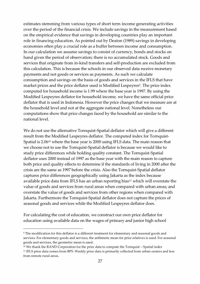
27

estimates stemming from various types of short term income generating activities

over the period of the financial crisis. We include savings in the measurement based

on the empirical evidence that savings in developing countries play an important

role in financing education. As pointed out by Deaton (1989) savings in developing

economies often play a crucial role as a buffer between income and consumption.

In our calculation we assume savings to consist of currency, bonds and stocks on

hand given the period of observation; there is no accumulated stock. Goods and

services that originate from in-kind transfers and self-production are excluded from

this calculation. This is because the schools in our observed data receive monetary

payments and not goods or services as payments. As such we calculate

consumption and savings on the basis of goods and services in the IFLS that have

market prices and the price deflator used is Modified Lespeyres9. The price index

computed for household income is 1.99 where the base year is 1997. By using the

Modified Lespeyres deflator for household income, we have the same official price

deflator that is used in Indonesia. However the price changes that we measure are at

the household level and not at the aggregate national level. Nonetheless our

computations show that price changes faced by the household are similar to the

national level.

We do not use the alternative Tornquist-Spatial deflator which will give a different

result from the Modified Lespeyres deflator. The computed index for Tornquist-

Spatial is 2.0610 where the base year is 2000 using IFLS data. The main reason that

we choose not to use the Tornquist-Spatial deflator is because we would like to

study price differences while holding quality constant. The Tornquist-Spatial

deflator uses 2000 instead of 1997 as the base year with the main reason to capture

both price and quality effects to determine if the standards of living in 2000 after the

crisis are the same as 1997 before the crisis. Also the Tornquist-Spatial deflator

captures price differences geographically using Jakarta as the index because

available price data from IFLS has an urban reporting bias11 which will overstate the

value of goods and services from rural areas when compared with urban areas; and

overstate the value of goods and services from other regions when compared with

Jakarta. Furthermore the Tornquist-Spatial deflator does not capture the prices of

seasonal goods and services while the Modified Lespeyres deflator does.

For calculating the cost of education, we construct our own price deflator for

education using available data on the wages of primary and junior high school

9 The modification for this deflator is a different treatment for elementary and seasonal goods and

services. For elementary goods and services, the arithmetic mean for price relatives is used. For seasonal

goods and services, the geometric mean is used. 10 We thank the RAND Corporation for the price data to compute the Tornquist – Spatial index 11 IFLS price data comes from BPS. Weekly price data is primarily collected from urban centers and less

from remote rural areas.

28

teachers that are in the same schools in the same communities in 1997 and 2000.

Data on other education costs is not available. The price index computed for

education is 2.47 where the base year is 1997. Wages are used because changes over

time are caused by the price effect and not the quality effect. The education price

deflator enables us to hold school quality reasonably constant in 1997 and 2000 to

isolate the pure income effect on education. One of the drawbacks of using teacher

wages is family educational spending is primarily for school fees and monthly

scheduled payments to cover school operational costs and not teacher wages.

However the cost of schooling related fees are nonetheless indirectly related to

teacher wages. We use this price deflator for education specifically covering primary

school and junior high instead of using the Modified Lespeyres deflator which is

computed using savings and all consumption goods including education at different

school levels.

Table 2.6 provides a summary of the different price indices. A review of these price

indices show that price changes for different consumer goods at the national

aggregate level are in a similar range as at the disaggregated household level. As

such our choice of the Modified Lespeyres deflator for household income and our

self-constructed priced deflator for education are robust for computing real prices.

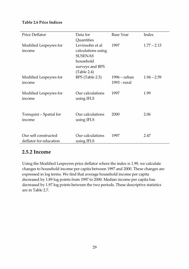
29

Table 2.6 Price Indices

Price Deflator Data for

Quantities

Base Year Index

Modified Lespeyres for

income

Levinsohn et al

calculations using

SUSENAS

household

surveys and BPS

(Table 2.4)

1997 1.77 – 2.13

Modified Lespeyres for

income

BPS (Table 2.5) 1996 – urban

1993 - rural

1.94 – 2.59

Modified Lespeyres for

income

Our calculations

using IFLS

1997 1.99

Tornquist – Spatial for

income

Our calculations

using IFLS

2000 2.06

Our self constructed

deflator for education

Our calculations

using IFLS

1997 2.47

2.5.2 Income

Using the Modified Lespeyres price deflator where the index is 1.99, we calculate

changes to household income per capita between 1997 and 2000. These changes are

expressed in log terms. We find that average household income per capita

decreased by 1.89 log points from 1997 to 2000. Median income per capita has

decreased by 1.97 log points between the two periods. These descriptive statistics

are in Table 2.7.

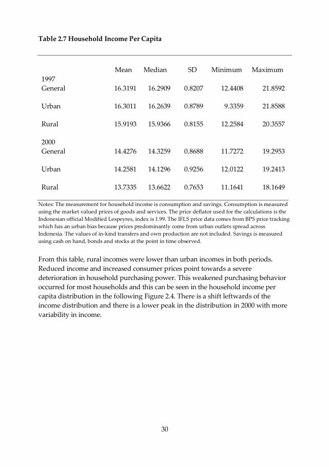
30

Table 2.7 Household Income Per Capita

Mean

Median SD Minimum Maximum

1997

General 16.3191 16.2909 0.8207 12.4408 21.8592

Urban 16.3011 16.2639 0.8789 9.3359 21.8588

Rural 15.9193 15.9366 0.8155 12.2584 20.3557

2000

General 14.4276 14.3259 0.8688 11.7272 19.2953

Urban 14.2581 14.1296 0.9256 12.0122 19.2413

Rural 13.7335 13.6622 0.7653 11.1641 18.1649

Notes: The measurement for household income is consumption and savings. Consumption is measured

using the market valued prices of goods and services. The price deflator used for the calculations is the

Indonesian official Modified Lespeyres, index is 1.99. The IFLS price data comes from BPS price tracking

which has an urban bias because prices predominantly come from urban outlets spread across

Indonesia. The values of in-kind transfers and own production are not included. Savings is measured

using cash on hand, bonds and stocks at the point in time observed.

From this table, rural incomes were lower than urban incomes in both periods.

Reduced income and increased consumer prices point towards a severe

deterioration in household purchasing power. This weakened purchasing behavior

occurred for most households and this can be seen in the household income per

capita distribution in the following Figure 2.4. There is a shift leftwards of the

income distribution and there is a lower peak in the distribution in 2000 with more

variability in income.

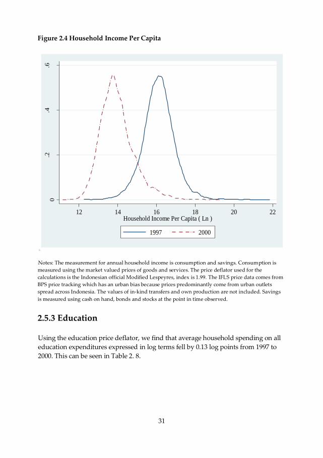
31

Figure 2.4 Household Income Per Capita

0.2

.4.6

12 14 16 18 20 22Household Income Per Capita ( Ln )

1997 2000

Notes: The measurement for annual household income is consumption and savings. Consumption is

measured using the market valued prices of goods and services. The price deflator used for the

calculations is the Indonesian official Modified Lespeyres, index is 1.99. The IFLS price data comes from

BPS price tracking which has an urban bias because prices predominantly come from urban outlets

spread across Indonesia. The values of in-kind transfers and own production are not included. Savings

is measured using cash on hand, bonds and stocks at the point in time observed.

2.5.3 Education

Using the education price deflator, we find that average household spending on all

education expenditures expressed in log terms fell by 0.13 log points from 1997 to

2000. This can be seen in Table 2. 8.

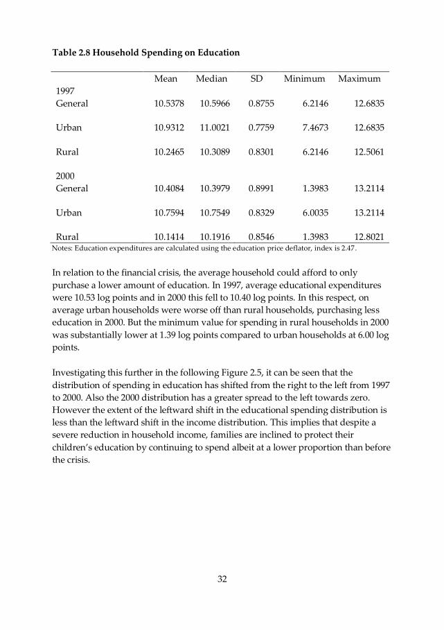
32

Table 2.8 Household Spending on Education

Mean Median SD Minimum Maximum

1997

General 10.5378 10.5966 0.8755 6.2146 12.6835

Urban 10.9312 11.0021 0.7759 7.4673 12.6835

Rural 10.2465 10.3089 0.8301 6.2146 12.5061

2000

General 10.4084 10.3979 0.8991 1.3983 13.2114

Urban 10.7594 10.7549 0.8329 6.0035 13.2114

Rural 10.1414 10.1916 0.8546 1.3983 12.8021 Notes: Education expenditures are calculated using the education price deflator, index is 2.47.

In relation to the financial crisis, the average household could afford to only

purchase a lower amount of education. In 1997, average educational expenditures

were 10.53 log points and in 2000 this fell to 10.40 log points. In this respect, on

average urban households were worse off than rural households, purchasing less

education in 2000. But the minimum value for spending in rural households in 2000

was substantially lower at 1.39 log points compared to urban households at 6.00 log

points.

Investigating this further in the following Figure 2.5, it can be seen that the

distribution of spending in education has shifted from the right to the left from 1997

to 2000. Also the 2000 distribution has a greater spread to the left towards zero.

However the extent of the leftward shift in the educational spending distribution is

less than the leftward shift in the income distribution. This implies that despite a

severe reduction in household income, families are inclined to protect their

children’s education by continuing to spend albeit at a lower proportion than before

the crisis.

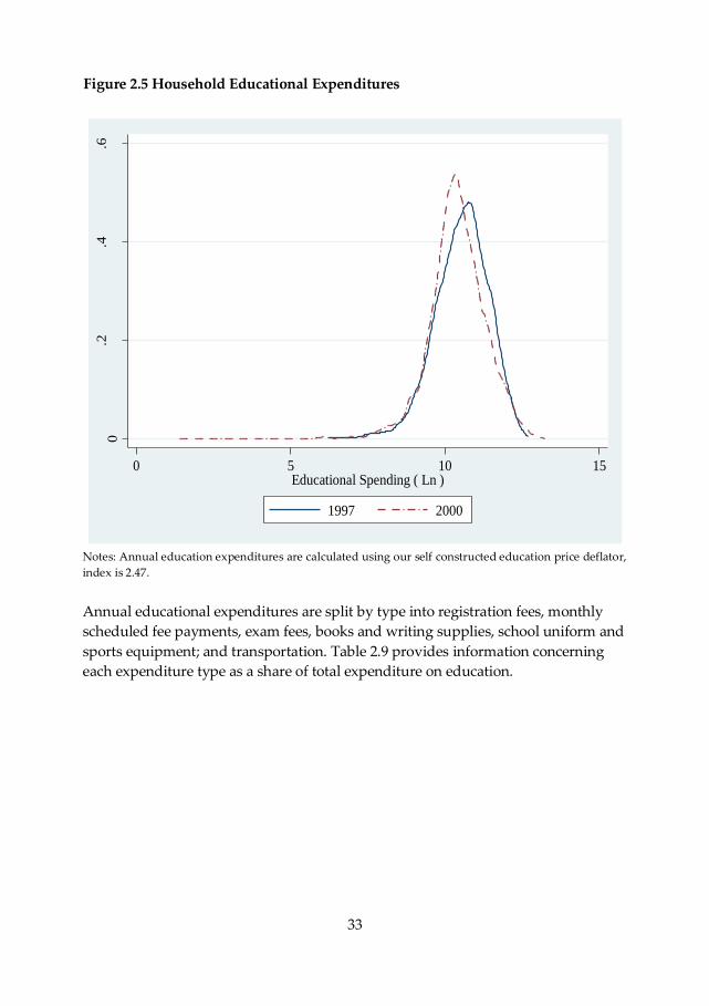
33

Figure 2.5 Household Educational Expenditures

0.2

.4.6

0 5 10 15Educational Spending ( Ln )

1997 2000

Notes: Annual education expenditures are calculated using our self constructed education price deflator,

index is 2.47.

Annual educational expenditures are split by type into registration fees, monthly

scheduled fee payments, exam fees, books and writing supplies, school uniform and

sports equipment; and transportation. Table 2.9 provides information concerning

each expenditure type as a share of total expenditure on education.

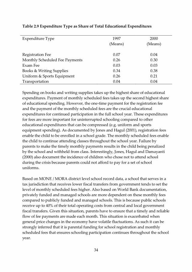
34

Table 2.9 Expenditure Type as Share of Total Educational Expenditures

Expenditure Type 1997

(Means)

2000

(Means)

Registration Fee

0.07

0.04

Monthly Scheduled Fee Payments 0.26 0.30

Exam Fee 0.03 0.03

Books & Writing Supplies 0.34 0.38

Uniform & Sports Equipment 0.26 0.21

Transportation 0.04 0.04

Spending on books and writing supplies takes up the highest share of educational

expenditures. Payment of monthly scheduled fees takes up the second highest share

of educational spending. However, the one-time payment for the registration fee

and the payment of the monthly scheduled fees are the crucial educational

expenditures for continued participation in the full school year. These expenditures

for fees are more important for uninterrupted schooling compared to other

educational expenditures that can be compressed (e.g. uniform and sports

equipment spending). As documented by Jones and Hagul (2001), registration fees

enable the child to be enrolled in a school grade. The monthly scheduled fees enable

the child to continue attending classes throughout the school year. Failure by

parents to make the timely monthly payments results in the child being penalized

by the school and withheld from class. Interestingly, Jones, Hagul and Damayanti

(2000) also document the incidence of children who chose not to attend school

during the crisis because parents could not afford to pay for a set of school

uniforms.

Based on MONE / MORA district level school record data, a school that serves in a

tax jurisdiction that receives lower fiscal transfers from government tends to set the

level of monthly scheduled fees higher. Also based on World Bank documentation,

privately funded and managed schools are more dependent on these monthly fees

compared to publicly funded and managed schools. This is because public schools

receive up to 40% of their total operating costs from central and local government

fiscal transfers. Given this situation, parents have to ensure that a timely and reliable

flow of fee payments are made each month. This situation is exacerbated when

general price changes in the economy have volatile fluctuations. As such it can be

strongly inferred that it is parental funding for school registration and monthly

scheduled fees that ensures schooling participation continues throughout the school

year.

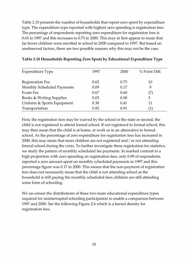
35

Table 2.10 presents the number of households that report zero spent by expenditure

type. The expenditure type reported with highest zero spending is registration fees.

The percentage of respondents reporting zero expenditure for registration fees is

0.65 in 1997 and this increases to 0.75 in 2000. This may at first appear to mean that

far fewer children were enrolled in school in 2000 compared to 1997. But based on

unobserved factors, there are two possible reasons why this may not be the case.

Table 2.10 Households Reporting Zero Spent by Educational Expenditure Type

Expenditure Type 1997 2000 % Point Diff.

Registration Fee 0.65 0.75 10

Monthly Scheduled Payments 0.09 0.17 9

Exam Fee 0.67 0.60 (7)

Books & Writing Supplies 0.03 0.08 5

Uniform & Sports Equipment 0.30 0.41 11

Transportation 0.92 0.91 (1)

First, the registration fees may be waived by the school or the state or second, the

child is not registered to attend formal school. If not registered in formal school, this

may then mean that the child is at home, at work or in an alternative to formal

school. As the percentage of zero expenditure for registration fees has increased in

2000, this may mean that more children are not registered and / or not attending

formal school during the crisis. To further investigate these registration fee statistics,

we study the pattern of monthly scheduled fee payments. In marked contrast to a

high proportion with zero spending on registration fees, only 0.09 of respondents

reported a zero amount spent on monthly scheduled payments in 1997 and this

percentage figure was 0.17 in 2000. This means that the non-payment of registration

fees does not necessarily mean that the child is not attending school as the

household is still paying the monthly scheduled fees; children are still attending

some form of schooling.

We un-censor the distributions of these two main educational expenditure types

required for uninterrupted schooling participation to enable a comparison between

1997 and 2000. See the following Figure 2.6 which is a kernel density for

registration fees.

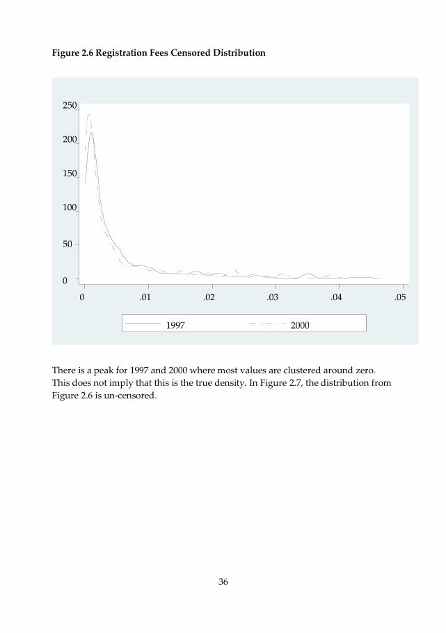
36

Figure 2.6 Registration Fees Censored Distribution

There is a peak for 1997 and 2000 where most values are clustered around zero.

This does not imply that this is the true density. In Figure 2.7, the distribution from

Figure 2.6 is un-censored.

0

50

100

150

200

250

0 .01 .02 .03 .04 .05

1997 2000

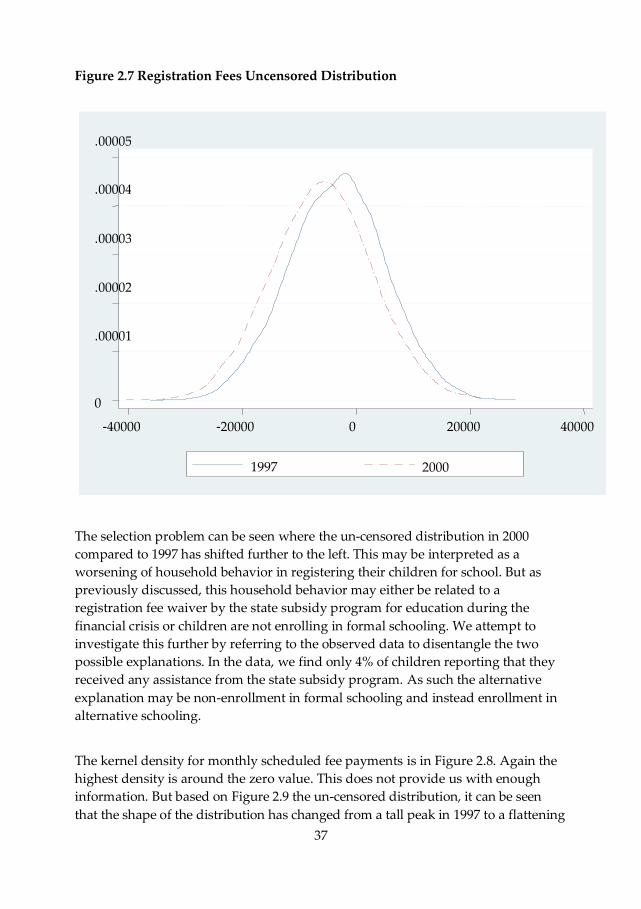
37

Figure 2.7 Registration Fees Uncensored Distribution

The selection problem can be seen where the un-censored distribution in 2000

compared to 1997 has shifted further to the left. This may be interpreted as a

worsening of household behavior in registering their children for school. But as

previously discussed, this household behavior may either be related to a

registration fee waiver by the state subsidy program for education during the

financial crisis or children are not enrolling in formal schooling. We attempt to

investigate this further by referring to the observed data to disentangle the two

possible explanations. In the data, we find only 4% of children reporting that they

received any assistance from the state subsidy program. As such the alternative

explanation may be non-enrollment in formal schooling and instead enrollment in

alternative schooling.

The kernel density for monthly scheduled fee payments is in Figure 2.8. Again the

highest density is around the zero value. This does not provide us with enough

information. But based on Figure 2.9 the un-censored distribution, it can be seen

that the shape of the distribution has changed from a tall peak in 1997 to a flattening

0

.00001

.00002

.00003

.00004

.00005

-40000 -20000 0 20000 40000

1997 2000

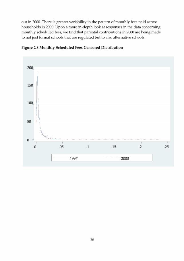
38

out in 2000. There is greater variability in the pattern of monthly fees paid across

households in 2000. Upon a more in-depth look at responses in the data concerning

monthly scheduled fees, we find that parental contributions in 2000 are being made

to not just formal schools that are regulated but to also alternative schools.

Figure 2.8 Monthly Scheduled Fees Censored Distribution

0

50

100

150

200

0 .05 .1 .15 .2 .25

1997 2000

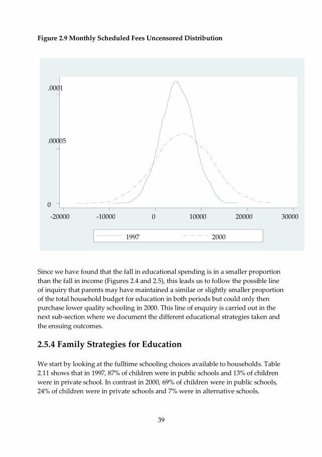
39

Figure 2.9 Monthly Scheduled Fees Uncensored Distribution

Since we have found that the fall in educational spending is in a smaller proportion

than the fall in income (Figures 2.4 and 2.5), this leads us to follow the possible line

of inquiry that parents may have maintained a similar or slightly smaller proportion

of the total household budget for education in both periods but could only then

purchase lower quality schooling in 2000. This line of enquiry is carried out in the

next sub-section where we document the different educational strategies taken and

the ensuing outcomes.

2.5.4 Family Strategies for Education

We start by looking at the fulltime schooling choices available to households. Table

2.11 shows that in 1997, 87% of children were in public schools and 13% of children

were in private school. In contrast in 2000, 69% of children were in public schools,

24% of children were in private schools and 7% were in alternative schools.

0

.00005

.0001

-20000 -10000 0 10000 20000 30000

1997 2000

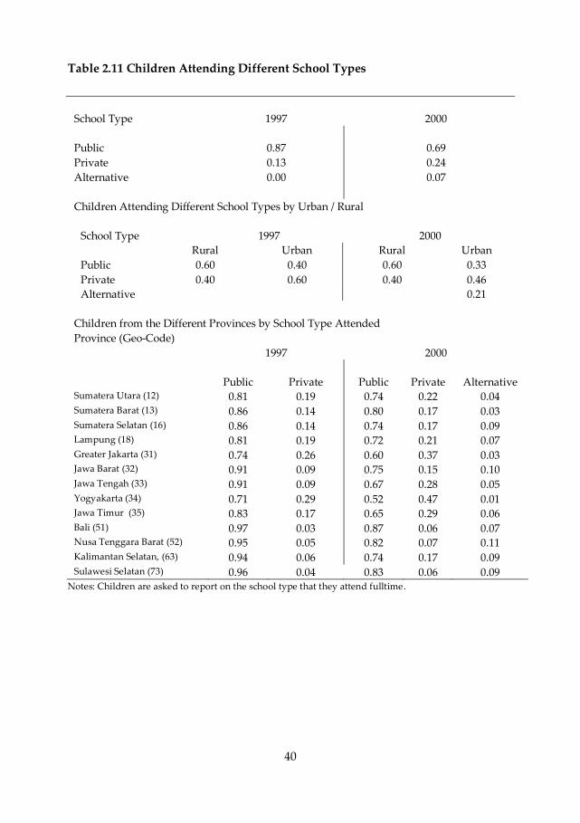
40

Table 2.11 Children Attending Different School Types

School Type 1997 2000

Public 0.87 0.69

Private 0.13 0.24

Alternative 0.00 0.07

Children Attending Different School Types by Urban / Rural

School Type 1997 2000

Rural Urban Rural Urban

Public 0.60 0.40 0.60 0.33

Private 0.40 0.60 0.40 0.46

Alternative 0.21

Children from the Different Provinces by School Type Attended

Province (Geo-Code)

1997

2000

Public

Private

Public

Private

Alternative Sumatera Utara (12) 0.81 0.19 0.74 0.22 0.04 Sumatera Barat (13) 0.86 0.14 0.80 0.17 0.03 Sumatera Selatan (16) 0.86 0.14 0.74 0.17 0.09 Lampung (18) 0.81 0.19 0.72 0.21 0.07 Greater Jakarta (31) 0.74 0.26 0.60 0.37 0.03 Jawa Barat (32) 0.91 0.09 0.75 0.15 0.10 Jawa Tengah (33) 0.91 0.09 0.67 0.28 0.05 Yogyakarta (34) 0.71 0.29 0.52 0.47 0.01 Jawa Timur (35) 0.83 0.17 0.65 0.29 0.06 Bali (51) 0.97 0.03 0.87 0.06 0.07 Nusa Tenggara Barat (52) 0.95 0.05 0.82 0.07 0.11 Kalimantan Selatan, (63) 0.94 0.06 0.74 0.17 0.09 Sulawesi Selatan (73) 0.96 0.04 0.83 0.06 0.09

Notes: Children are asked to report on the school type that they attend fulltime.

41

In the IFLS surveys in both years, households were asked to write down the type of

schooling received if the other closed ended school type options (formal public or

private schools) did not apply. We determined these open ended written

descriptions to be alternative ways of learning which corresponds to descriptions

provided by MONE and MORA in Section 2.2.2 and Figure 2.3. We add this

alternative method into the portfolio of school choice. As argued by Heckman and

Lochner (2000), we recognize non-institutional sources of skill formation like

families, neighborhoods and firms to be as important as the formal school system

for learning. Alternative schooling and the characteristics of children who attend

these schools such as child laborers and child apprentices will be examined further

in Chapter 4.

From Table 2.11, in terms of the urban-rural split, in 1997 60% of children from

rural households went to public school and 40% went to private school. For urban

children, the reverse pattern occurred where 40% went to public school and 60%

went to private school in 1997. In 2000 the rural household public – private school

split remained the same as in 1997. But there were changes for children from urban

households. In 2000, 33% of urban children were in public school; 46% of urban

children were in private school and 21% of urban children were in a third type being

alternative school.

32% of total observed alternative schools in Indonesia were located in Java and Bali

Islands and the rest split up between the Outer Islands. Because of modernization

and consequently urbanization, Java and Bali Islands have attracted the majority of

the population. Java and Bali based on BPS estimates in 2003 is home to 60% of the

total country population but represents less than 7% of total land mass in

Indonesia. Particularly the urbanization of Java is seen through the greater Jakarta

area which is characterized by slum dwellings and landless labor and this is

documented by BPS. Perhaps the majority population in Java and Bali has promoted

the availability of more alternative schooling choices.

From these findings it is inferred that given the larger school type choice available to

urban households, they had various ways to adjust their behavior when income fell.

It is posited that parents could look for market driven solutions (unregulated by

MONE and MORA) to maintain their children's education. Given these different

strategies, households appear to vary the amount of school quality that they can

afford to purchase. They choose to substitute between low quality and high quality

schools. One of the possible consequences is the increased incidence of children

attending low quality non-formal and informal schools while working. In the next

section, we study whether this substitution in schooling quality has negatively

affected the children in terms of educational outcomes.

42

2.5.5 Quality of Educational Outcomes

Based on the observed data, there are EBTANAS test scores for children who on the

basis of their scores have qualified to transition from formal primary school to

formal junior high school. This means that in 1997, we have test scores for children

who were at the junior high level. This level of schooling consists of three years. As

such there are score records for students in the first, second or third year in this

level. For a student in the first year of junior high in 1997, his / her test score is from

1996. For a student in the second year, the score is from 1995. For the third year, the

score is from 1994. The same sequence applies to 2000 for the first, second and third

school years being 1999, 1998 and 1997 respectively. We use EBTANAS to study

which children succeeded or failed to transition and relate this to the period of the

financial crisis. We use this measure of transition instead of years of schooling

because entry into the Indonesian formal labor market is primarily determined by

completion of successive school levels.12 As such the school level completed instead

of schooling years completed is a more valid measure of human capital

accumulation.

From the following Table 2.12, we find that there are two types of schooling

behavior in the observed data. The first type consists of children who completed

primary school, took EBTANAS and transitioned to junior high. The second type

consists of children who completed primary school, took EBTANAS but failed to

transition to junior high. For both periods, children who chose to transition have

higher average test scores than children who do not transition. This suggests that

higher ability children selected to progress on to junior high.

12 The level after SMP is senior high school for minimum entry into the formal labor market.

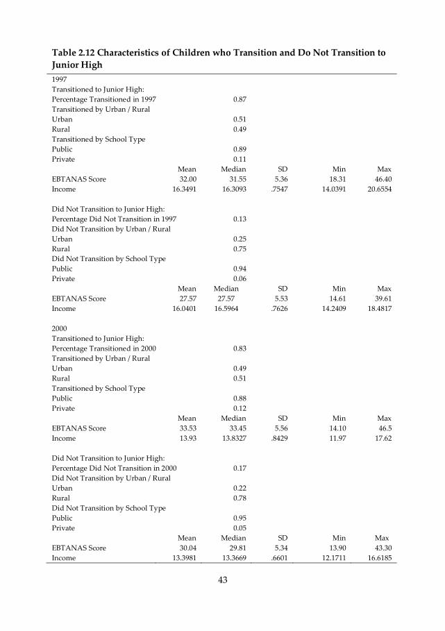
43

Table 2.12 Characteristics of Children who Transition and Do Not Transition to

Junior High

1997

Transitioned to Junior High:

Percentage Transitioned in 1997 0.87

Transitioned by Urban / Rural

Urban 0.51

Rural 0.49

Transitioned by School Type

Public 0.89

Private 0.11

Mean Median SD Min Max

EBTANAS Score 32.00 31.55 5.36 18.31 46.40

Income 16.3491 16.3093 .7547 14.0391 20.6554

Did Not Transition to Junior High:

Percentage Did Not Transition in 1997 0.13

Did Not Transition by Urban / Rural

Urban 0.25

Rural 0.75

Did Not Transition by School Type

Public 0.94

Private 0.06

Mean Median SD Min Max

EBTANAS Score 27.57 27.57 5.53 14.61 39.61

Income 16.0401 16.5964 .7626 14.2409 18.4817

2000

Transitioned to Junior High:

Percentage Transitioned in 2000 0.83

Transitioned by Urban / Rural

Urban 0.49

Rural 0.51

Transitioned by School Type

Public 0.88

Private 0.12

Mean Median SD Min Max

EBTANAS Score 33.53 33.45 5.56 14.10 46.5

Income 13.93 13.8327 .8429 11.97 17.62

Did Not Transition to Junior High:

Percentage Did Not Transition in 2000 0.17

Did Not Transition by Urban / Rural

Urban 0.22

Rural 0.78

Did Not Transition by School Type

Public 0.95

Private 0.05

Mean Median SD Min Max

EBTANAS Score 30.04 29.81 5.34 13.90 43.30

Income 13.3981 13.3669 .6601 12.1711 16.6185

44

Also average test scores overall are higher in 2000 compared to 1997. But there is a

larger spread of scores in 2000 compared to 1997. In 2000, 17% of students did not

sit for all 5 tests compared to 1997 where only 1% of students did not sit for all

tests13. This affected the lower bound of the cumulative test score reported in 2000.

The second type of schooling behavior, qualifying but not transitioning was also

observed by Suryadarma, Suryahadi and Sumarto (2006). They investigate the

causes of low junior high enrollment despite near universal primary school

attendance. They find that attrition during the transition between primary school

and junior high is the main cause. Our findings concerning this second type of

schooling behavior can be seen in Table 2.11 and the following Figure 2.10.

13 We carried out tabulations for the EBTANAS test scores by of the five individual subjects but do not

report them in this chapter.

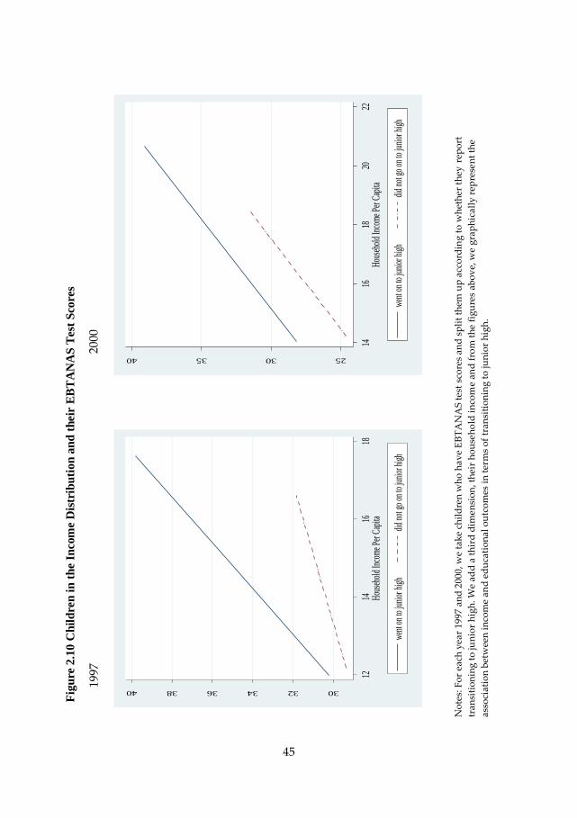
45

25303540

EBTANAS Score

1416

1820

22H

ouse

hold

Inco

me

Per C

apita

wen

t on

to ju

nior

hig

hdi

d no

t go

on to

juni

or h

igh

303234363840

EBTANAS Score

1214

1618

Hou

seho

ld In

com

e Per

Cap

ita

wen

t on

to ju

nior

hig

hdi

d no

t go

on to

juni

or h

igh

No

tes:

Fo

r ea

ch y

ear

19

97

an

d 2

00

0, w

e ta

ke

chil

dre

n w

ho

ha

ve

EB

TA

NA

S t

est

sco

res

an

d s

pli

t th

em u

p a

cco

rdin

g t

o w

het

her

th

ey r

epo

rt

tra

nsi

tio

nin

g t

o ju

nio

r h

igh

. W

e a

dd

a t

hir

d d

ime

nsi

on

, th

eir

ho

use

ho

ld i

nco

me

an

d f

rom

th

e f

igu

res

ab

ov

e, w

e g

rap

hic

all

y r

epre

sen

t th

e

ass

oci

ati

on

bet

wee

n i

nco

me

an

d e

du

cati

on

al

ou

tco

mes

in

ter

ms

of

tra

nsi

tio

nin

g t

o ju

nio

r h

igh

.

1997

20

00

Fig

ure

2.1

0 C

hil

dre

n i

n t

he

Incom

e D

istr

ibu

tio

n a

nd

th

eir

EB

TA

NA

S T

est

Sco

res

46

In Figure 2.10, for each year observed, we split children with EBTANAS test scores

into two groups by whether they qualified and transitioned to junior high or not.

As seen first in Table 2.12 and then in Figure 2.10, there are then two groups each

for 1997 and 2000 and their position in the household income distribution.

Children who qualify but do not transition to junior high in both periods are fewer

than those who do qualify and transition. But when comparing the percentage of

all qualified children who do not transition for 1997 and 2000, we find a

deterioration of this outcome in 2000. In 2000, 30% more children qualified but did

not transition compared to 1997.

In the observed data a majority of almost 90% of the children who transition come

from public schools and this appears to be a naturally occurring trend because the

same proportion is seen in both periods. This may because most children select

into public schools because of higher quality than private schools and this is also

observed by Newhouse and Beegle (2005). When viewed in terms of the income

distribution, in 2000, the non-transitioned children come from households with

lower incomes than in 1997. In Figure 2.10, upon further investigation there is a

greater distance in test scores between non-transitioned and transitioned children

in 2000. In 1997 children up to the 50th percentile of the distribution did not

transition. But in 2000 this became worse where children all the way up to the 60 th

percentile of the distribution did not transition to junior high. Since these children

were still in primary school in the prior crisis years of 1998 and 1999, it can be

inferred that reduced household incomes for up to the 60th percentile resulted in

failure to transition to junior high. Also it may appear that some of these children

chose alternative schooling which would have compromised their eligibility to sit

for EBTANAS.

2.6 Conclusions In this chapter we documented family spending behavior adjusting to an

unanticipated reduction in household income. We find that the amount of

education that is purchased is reduced and in relation to this, the quality of

educational outcomes over the period of the AFC is compromised. By analyzing

un-censored distributions for education related expenditures, we are able to

document and infer unobserved differences in education spending behavior. It is

found that parents used various strategies to maintain their children’s schooling

participation – struggling to keep up with making timely monthly scheduled fee

payments, substituting between public and private school, choosing alternative

schooling and deciding for their children to combine work with learning. The

ability of the child on the basis of EBTANAS test scores is also a factor that parents

47

took into consideration where children with a better educational performance

qualified and transitioned to junior high. But despite the different education

strategies taken there were children with household incomes up to the 60th

percentile who qualified but did not transition to junior high. This raises the

question whether the children continued their formal education later in time after

the AFC or never resumed their formal schooling.

The effects of the AFC washed away relatively quickly at the macroeconomic level.

But we argue that given the empirics on family background and intergenerational

mobility (Becker and Tomes, 1964), such associated effects can be profound in

terms of labor market outcomes and social changes. By losing out even temporarily

on a quality education in the formal education system, there may be a generation of

children who have come of age now a decade later and unable to effectively

compete in the formal labor market. Or this generation of children may have lost

out on further building socially productive skills.

Given this documentation and our arguments, we have provided justification for

the use of the AFC as an instrumental variable that is relevant and exogenous. We

show that the AFC is relevant because it is correlated with income and it is

plausibly exogenous because it is not directly correlated with educational spending

but through its correlation with income. As such we will use the AFC as an

instrumental variable in Chapters 4 and 5. However we are fully cognizant of the

possibility of the differential effects of the AFC on education across the archipelago.

As such we will examine this aspect of regional variation in Chapter 3.

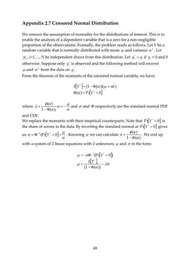
48

Appendix 2.7 Censored Normal Distribution

We remove the assumption of normality for the distributions of interest. This is to

enable the analysis of a dependent variable that is a zero for a non-negligible

proportion of the observations. Formally, the problem reads as follows. Let Y be a

random variable that is normally distributed with mean and variance 2 . Let

iy , i=1,…, N be independent draws from this distribution. Let ii yy * if

iy > 0 and 0

otherwise. Suppose only *

iy is observed and the following method will recover

and 2 from the data on *

iy

From the theorem of the moments of the censored normal variable, we have:

0Pr)(

)))((1(*

*

Y

YE

where

),(1

)(and and respectively are the standard normal PDF

and CDF.

We replace the moments with their empirical counterparts. Note that 0Pr * Y is

the share of zeroes in the data. By inverting the standard normal at 0Pr * Y gives

us

0(Pr *1 Y . Knowing we can calculate

)(1

)(

. We end up

with a system of 2 linear equations with 2 unknowns and in the form:

))(1(

)0(Pr*

*1

YE

Y

49

3. Electricity Access, Use and Children’s

Educational Performance

50

3.1 Introduction

In developing countries, promoting schooling includes establishing and

maintaining physical infrastructure. One of these basic facilities is the availability of

electricity in the school and the household. This enables children to learn efficiently

where studying can take place in both the classroom and at home. Doing

homework and study revision at home complements classroom instruction.

However in a large developing country like Indonesia, there is wide regional

variation in the distribution of electricity where underdeveloped areas have less

access to electricity compared to industrial and growth areas. Unequal access to

electricity is a potential constraint for educational performance.

The aim of this chapter is to study the proposed correlational relationship between

the availability and use of electricity and educational performance; given regional

variation14. We investigate the standardized achievement test scores of Indonesian

children aged 12 where we exploit variation in the availability and in the use of

electricity in the school and the household across different communities. We

examine whether available electricity is used as electric light for learning or

whether different uses of electricity influence outcomes. We study the children’s

educational performance using test scores for two periods, 1997 and 2000.

In the literature, Glewwe and Kremer (2005) write about the wide variation in

educational input levels and education systems across developing countries which

affect the quality of schooling. Teachers are often absent from classrooms and many

children learn much less than the learning objectives set in the official curriculum

(Lockheed and Verspoor, 1991; Harbison and Hanushek, 1992; Hanuskek, 1995;

Glewwe, 1999). Also many schools lack the most basic equipment and school

supplies and sometimes even classrooms, in which case classes meet outside and

are cancelled when it rains (World Bank, 1997 and Glewwe, 2004). But Kremer et al

(2005) find that in India one of the positive correlates of teacher presence is school

infrastructure which represents better working conditions. In Honduras, Bedi and

Marshall (2001) find that better school facilities increase primary school attendance.

Also Alatas (2000) finds that the introduction of basic infrastructure in left behind

villages in Indonesia improves school enrollment. More specifically, Bacalod and

Tobias (2006) find that minimal basic facilities in the school, particularly electricity

matter more for test score performance in the Philippines than class size and

teacher training programs. This chapter contributes to this strand of the literature

by focusing on the availability and use of electricity in the school and household in

Indonesia on educational achievement.

14 This chapter does not use the Asian Financial Crisis as an instrument and instead focuses on regional

variation.

51

The rest of the paper is set up in the following way. Section 3.2 provides a

description of the energy sector in Indonesia and how electric energy is delivered

from the source to the final user. This description consists of the layout of the

energy sources, power plants and transmission lines in the main islands. We also

include the distribution trends for industrial, household (including school) and

transport use. Section 3.3 provides a description of schooling provision in

Indonesia and how school quality is documented by the national school census.

Section 3.4 covers the empirical specification and the data we use, the Indonesian

Family Life Surveys (IFLS). In Section 3.5 we provide descriptive statistics followed

by results in Section 3.6. Conclusions are made in Section 3.7.

3.2 The Energy Sector in Indonesia

According to the Energy Information Administration of the US Government which

compiles energy statistics from around the world, Indonesia’s power generation

sector is dominated by the state-owned electric utility PT PLN (Persero), formerly

known as Perusahaan Listrik Negara. The history of PT PLN in Indonesia began at

the end of 19th century stemming from the Dutch East India Company establishing

power generation for its trading interests in certain geographical areas in the

archipelago. The electrical energy enterprise then expanded into the public interest

company, NV.NIGM. In World War II, the Japanese seized control of the electric

companies. After Indonesian Independence in 1945 the Republic of Indonesia

assumed ownership of the energy infrastructure. PT PLN operates 45 power plants

and transmission lines for on-grid energy supply, or roughly two-thirds of the

country’s generating capacity.

Indonesia’s electricity sector faces severe underinvestment, and the country’s

energy officials have set out on a program to expand generation capacity. The

consequences of underinvestment are bottlenecks in provincial level

interconnections between bulk transmission and sub-transmission levels,

overloading and voltage problems at sub-transmission levels (World Bank, 2003).

The bottlenecks in provincial level interconnections negatively affect the efficient

transmission of electric power. As such the outcome of transmission inefficiencies

is uneven and interrupted electricity transmission. These interruptions can

manifest themselves in terms of brownouts where there is a drop in voltage and

lights dim and / or; blackouts where there is a total loss of power.

One of the major obstacles to increasing Indonesia’s power generating capacity is

pricing. The government sets the price at which PT PLN sells electricity in the

country. In relation to the Asian Financial Crisis, from end 1997 – end 2006 the

central government suspended PT PLN automatic tariff adjustments annually for

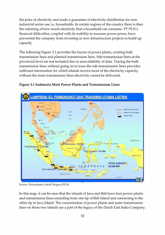
52

the price of electricity and made a guarantee of electricity distribution for non-

industrial sector use i.e. households. In certain regions of the country there is then

the rationing of how much electricity that a household can consume. PT PLN’s

financial difficulties, coupled with its inability to increase power prices, have

prevented the company from investing in new infrastructure projects to build up

capacity.

The following Figure 3.1 provides the layout of power plants, existing bulk

transmission lines and planned transmission lines. Sub-transmission lines at the

provincial level are not included due to unavailability of data. Tracing the bulk

transmission lines without going on to trace the sub-transmission lines provides

sufficient information for which islands receive most of the electricity capacity;

without the main transmission lines electricity cannot be delivered.

Figure 3.1 Indonesia Main Power Plants and Transmission Lines

Source: Perusahaan Listrik Negara (PLN)

In this map, it can be seen that the islands of Java and Bali have four power plants

and transmission lines extending from one tip of Bali Island and connecting to the

other tip in Java Island. The concentration of power plants and main transmission

lines on these two islands are a part of the legacy of the Dutch East India Company.

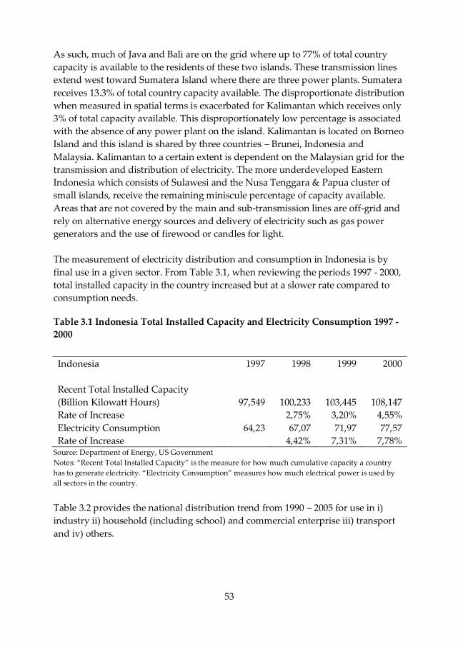
53

As such, much of Java and Bali are on the grid where up to 77% of total country

capacity is available to the residents of these two islands. These transmission lines

extend west toward Sumatera Island where there are three power plants. Sumatera

receives 13.3% of total country capacity available. The disproportionate distribution

when measured in spatial terms is exacerbated for Kalimantan which receives only

3% of total capacity available. This disproportionately low percentage is associated

with the absence of any power plant on the island. Kalimantan is located on Borneo

Island and this island is shared by three countries – Brunei, Indonesia and

Malaysia. Kalimantan to a certain extent is dependent on the Malaysian grid for the

transmission and distribution of electricity. The more underdeveloped Eastern

Indonesia which consists of Sulawesi and the Nusa Tenggara & Papua cluster of

small islands, receive the remaining miniscule percentage of capacity available.

Areas that are not covered by the main and sub-transmission lines are off-grid and

rely on alternative energy sources and delivery of electricity such as gas power

generators and the use of firewood or candles for light.

The measurement of electricity distribution and consumption in Indonesia is by

final use in a given sector. From Table 3.1, when reviewing the periods 1997 - 2000,

total installed capacity in the country increased but at a slower rate compared to

consumption needs.

Table 3.1 Indonesia Total Installed Capacity and Electricity Consumption 1997 -

2000

Indonesia 1997 1998 1999 2000

Recent Total Installed Capacity

(Billion Kilowatt Hours) 97,549 100,233 103,445 108,147

Rate of Increase 2,75% 3,20% 4,55%

Electricity Consumption 64,23 67,07 71,97 77,57

Rate of Increase 4,42% 7,31% 7,78% Source: Department of Energy, US Government

Notes: “Recent Total Installed Capacity” is the measure for how much cumulative capacity a country

has to generate electricity. “Electricity Consumption” measures how much electrical power is used by

all sectors in the country.

Table 3.2 provides the national distribution trend from 1990 – 2005 for use in i)

industry ii) household (including school) and commercial enterprise iii) transport

and iv) others.

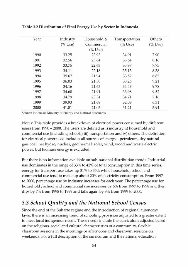
54

Table 3.2 Distribution of Final Energy Use by Sector in Indonesia

Year Industry

(% Use)

Household &

Commercial

(% Use)

Transportation

(% Use)

Others

(% Use)

1990 33.25 23.93 34.91 7.90

1991 32.56 23.64 35.64 8.16

1992 33.75 22.63 35.87 7.75

1993 34.11 22.18 35.13 8.58

1994 35.67 21.94 33.52 8.87

1995 36.03 21.50 33.26 9.21

1996 34.16 21.63 34.43 9.78

1997 34.60 21.91 33.98 9.52

1998 34.79 23.34 34.71 7.16

1999 39.93 21.68 32.08 6.31

2000 41.81 21.05 31.21 5.94 Source: Indonesia Ministry of Energy and Natural Resources

Notes: This table provides a breakdown of electrical power consumed by different

users from 1990 – 2000. The users are defined as i) industry ii) household and

commercial use (including schools) iii) transportation and iv) others. The definition

for electrical power used includes all sources of energy - petroleum, dry natural

gas, coal, net hydro, nuclear, geothermal, solar, wind, wood and waste electric

power. But biomass energy is excluded.

But there is no information available on sub-national distribution trends. Industrial

use dominates in the range of 33% to 42% of total consumption in this time series;

energy for transport use takes up 31% to 35% while household, school and

commercial use tend to make up about 20% of electricity consumption. From 1997

to 2000, percentage use by industry increases for each year. The percentage use for

household / school and commercial use increases by 6% from 1997 to 1998 and then

dips by 7% from 1998 to 1999 and falls again by 3% from 1999 to 2000.

3.3 School Quality and the National School Census Since the end of the Suharto regime and the introduction of regional autonomy

laws, there is an increasing trend of schooling provision adjusted to a greater extent

to meet local indigenous needs. These needs include the curriculum adjusted based

on the religious, social and cultural characteristics of a community, flexible

classroom sessions in the mornings or afternoons and classroom sessions on

weekends. For a full description of the curriculum and the national education

55

system, refer to Chapter 2. Geographic factors in relation to building schools and

maintaining school quality also have to be taken into consideration. As such

schools that are regulated and managed by MONE and MORA are registered in the

national school census. To ensure that the registered schools maintain a minimum

standard of school quality such as the level of teacher qualification and the

availability of teaching and learning material, there is also a checklist for required

physical school conditions that will promote an effective learning environment. The

checklist is in Table 3.3.

Table 3.3 MONE / MORA School Census Data – School Conditions Checklist

1. What is the number of seats in the classroom? (If one bench can be used for

6 students, then the count is 6 seats)

2. Are the blackboards, chalk and erasers in the classroom usable?

3. Is teaching in this classroom ever disrupted by inadequate lighting from

the main source of light, like window, door and opening?

4. Does the classroom use any electric lighting?

5. If yes, what is the main source of electricity?

PLN

Local Government Agency

School Generator

Social Self Reliance

Private Company or Cooperative

6. Did this classroom ever lose electrical power, and did this disrupt the

study activities?

7. When disruptions occur, is a substitute electricity source available?

8. Describe the floor of the classroom

9. Describe the walls in this classroom

10. Describe the roof used in this classroom

11. During the rainy season, did this classroom experience problems with:

leakage / floods / flash rains

56

Ensuring that schools have physical conditions that meet the minimum standards

of school quality is considered a pressing issue for schools serving in the central

government designated INPRES Desa Tertinggal (IDT) or Villages Left Behind

Program. This redistribution program is designed to identify underdeveloped

villages for the reduction of regional inequality. These neglected villages tend to be

characterized as being underdeveloped communities that include farm laborers,

peasants, fishermen, forest dwellers and young dropouts. These villages are

classified as left behind using population statistics; data on the village’s local

economic characteristics; whether the local population lives below the poverty line;

and the presence or absence of basic infrastructure and provincial government

provided facilities such as health services, schools, marketplaces, potable water,

electricity, and roads.15 Based on the program’s statistics, 94% of the villages

classified as IDT are located in rural areas. The 6% located in urban areas are in

slums. Because of underdevelopment, school quality in IDT villages is lower than

schools that are not serving in IDT villages. Consequently children’s educational

performance in IDT villages is very likely to be negatively affected.

3.4 Empirical Strategy

The dependent variable is educational performance as measured by the children’s

standardized achievement tests EBTANAS taken at the school age of 12. EBTANAS

assesses the child’s historical performance from age 6/7 at grade 116, to age 12 at

grade 6. EBTANAS is used to assess cognitive skills in the Indonesian language,

math, science, social studies and religious studies. The maximum score possible for

EBTANAS is 50 points. We compare the children’s EBTANAS educational

performance over two periods, 1997 and 2000 using pooled cross sections. We

investigate whether there exists a relationship between the availability of electricity

and electricity use in schools and households within a community and the child’s

educational performance. As our investigation is carried out when the Asian

Financial Crisis occurred in 1998, 1999 and to some extent in 2000, we factor this

context into our analysis.

We carry out the analysis at the community level which consists of the child’s

school and home. Our sample is restricted to communities that have schools and

households that report on whether they have access to electricity or not, if yes the

source of electricity (on the grid or off grid) and subsequently electricity use. We do

not have sufficient observations for schools that have access to the other types of

school infrastructure as described in Table 3.3. As such the sample is restricted to

15 The selection of villages into the program will also be politically driven and this was pointed out by

Perdana and Maxwell (2004). But our main consideration is the classification of this set of villages which

we will use in our empirical specification to identify villages that have low access to electricity. 16 While the starting school age for primary school is 7 years old, some children start at 6 years old.

57

electricity access in the school as well as in the household. We start with an OLS

base specification consisting of teacher quality, textbook loans to students and IDT

schools as educational inputs explaining the child’s educational achievement. From

IFLS, textbook loans are represented by Indonesian language and Math textbooks

only. The IDT variable represents underdevelopment in the child’s school and

household where there is only basic infrastructure available. The IDT variable is

then a proxy for low access to electricity. This is because in IFLS there is no data

available on the number of watts used in each community and there is no data on

the frequency of blackouts and brownouts. This base specification is similar to

Glewwe and Jacoby (1995) who attempt to isolate the school based determinants of

school achievement – teacher experience, the availability of textbooks and the

physical quality of a school. Also we include the availability of textbooks following

findings by Newhouse and Beegle (2005) where public schools in Indonesia that

have textbooks available for use are of higher quality. The number of sub-

transmission lines and connections to the national PLN grid in IDT are lower than

in developed communities. It is then more likely that schools and households in an

IDT community have low access (number of connections, volume and frequency) to

electricity compared to other communities that have high access to electricity. Also

the IDT variable is highly likely to be associated with low quality of educational

inputs compared to a developed community. That is, there may be fewer highly

qualified teachers who are willing to be posted to an underdeveloped community

and the latest textbooks may not be easily available.

We then expand the OLS base specification to include the endogenous explanatory

variables family income and the amount of the family budget allocated for

educational expenses. We do this to determine if the family has any role in

influencing test score variation. Then we introduce various variables measuring

electricity access and use to determine if there exists a relationship between

electricity and educational performance, after controlling for the child’s school

characteristics, household characteristics and underdevelopment in the community

(IDT).

We add an island control variable to the specification where a community is

located in Java and Bali Islands or not because of the placement of the grid and the

main transmission lines across the Main Islands. As 77% of the country’s total

energy capacity (both on-grid and off-grid) is available to Java and Bali,

communities located on these two islands are more likely to have access to

electricity as opposed to communities in Sumatera, Kalimantan, Sulawesi and the

cluster of small islands in Nusa Tenggara and Papua. The bulk of energy capacity

available on these two main islands also demonstrates that the major concentration

of economic activity, 60% of the country’s GDP is in Java and Bali (Hill, 1992; Hill et

al, 2008) In addition, we add a control variable for the community being located in

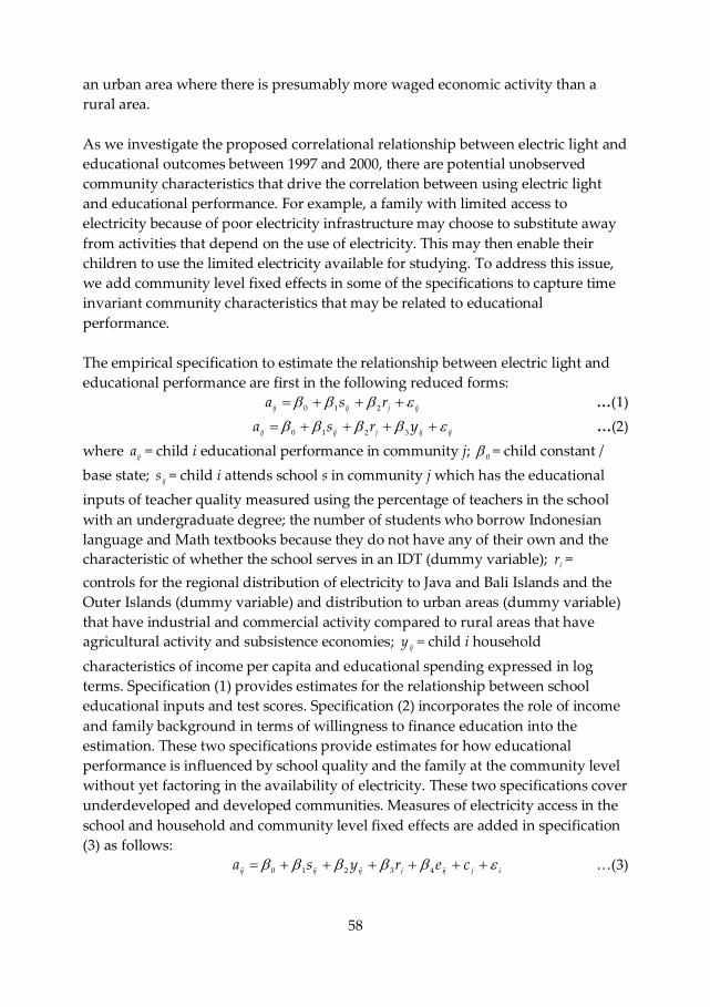
58

an urban area where there is presumably more waged economic activity than a

rural area.

As we investigate the proposed correlational relationship between electric light and

educational outcomes between 1997 and 2000, there are potential unobserved

community characteristics that drive the correlation between using electric light

and educational performance. For example, a family with limited access to

electricity because of poor electricity infrastructure may choose to substitute away

from activities that depend on the use of electricity. This may then enable their

children to use the limited electricity available for studying. To address this issue,

we add community level fixed effects in some of the specifications to capture time

invariant community characteristics that may be related to educational

performance.

The empirical specification to estimate the relationship between electric light and

educational performance are first in the following reduced forms:

ijjijij rsa 210 …(1)

ijijjijij yrsa 3210 …(2)

where ija = child i educational performance in community j; 0 = child constant /

base state; ijs = child i attends school s in community j which has the educational

inputs of teacher quality measured using the percentage of teachers in the school

with an undergraduate degree; the number of students who borrow Indonesian

language and Math textbooks because they do not have any of their own and the

characteristic of whether the school serves in an IDT (dummy variable); ir =

controls for the regional distribution of electricity to Java and Bali Islands and the

Outer Islands (dummy variable) and distribution to urban areas (dummy variable)

that have industrial and commercial activity compared to rural areas that have

agricultural activity and subsistence economies; ijy = child i household

characteristics of income per capita and educational spending expressed in log

terms. Specification (1) provides estimates for the relationship between school

educational inputs and test scores. Specification (2) incorporates the role of income

and family background in terms of willingness to finance education into the

estimation. These two specifications provide estimates for how educational

performance is influenced by school quality and the family at the community level

without yet factoring in the availability of electricity. These two specifications cover

underdeveloped and developed communities. Measures of electricity access in the

school and household and community level fixed effects are added in specification

(3) as follows:

ijijjijijij cerysa 43210 <(3)

59

where ije school and household have access to electricity in community j (dummy

variables); jc = fixed effects to capture time-invariant community characteristics

that may be related to educational outcomes. There is a small percentage of missing

values for the electricity access variables which we do not drop. Finally

specification (4) introduces the interaction between community underdevelopment,

electricity availability and electricity use as follows:

ijjijijijjijijij csuuerysa 6543210 <(4)

where iju = uses of electricity in the school and the household in community j

(dummy variables); ijsu = the interaction of the school characteristic of serving in an

IDT (Left Behind Village) with electricity use in school and at home in community

j. The interpretation of 6 is the number of EBTANAS points increased that is

explained by the availability of electricity in the child’s school and home and

electricity use for schooling and learning (low availability, low use if IDT, high

availability, high use if not IDT).

The data that we use is the RAND Corporation Indonesian Family Life Surveys

(IFLS) Waves 2 – 1997 and 3 – 2000. In IFLS, there is information on family income

and family spending on education. Educational expenditures are detailed by

expenditure types and whether spending is on a one time basis in the year or a

monthly flow of payments throughout the school year. The expenditure types

consist of registration fees, scheduled fee payment / contributions to the school,

textbooks for each course taken, writing supplies, uniforms, transportation costs,

private tuition, special courses and field trips. There is also a detailed description of

the household’s physical living environment; and whether it has any electricity

connection, a television and a refrigerator to store perishable food. Watching

television may be of indirect if not direct educational value which we will include

in our analysis. We exclude the refrigerator variable from our estimations because

the IFLS question is concerned with the use of the refrigerator to store perishable

food. There is no direct relationship with education. This dataset also provides

information on schooling inputs which consists of teachers, textbooks and

classrooms equipped with electricity. The data on schooling inputs is the same as

the MONE / MORA school census data. The questionnaire for the school physical

conditions component can be seen in Table 3.3. In the data there is also the child’s

officially reported EBTANAS test scores. The regional variables that we use from

the data are by island, community, urban / rural and whether the village is

underdeveloped (IDT).

We merge the variables of interest for community level of analysis using available

identifiers for the school, the household and the child. Because children can shift

between available schools of close proximity within the same community, we do

not observe the same individual children from the same household and from the

60

same school over the two periods of time. Also we do not observe a large sample of

the same households17 with two siblings the older aged 12 and the younger aged 9

in 1997 or aged 12 and 9 in 2000. As such we use the two pooled cross sections to

observe children from a given household attending school within a given

community. In addition, the use of repeated cross sections increases sample size

and power for analysis.

The main potential concern faced is the endogenous explanatory variables

representing where the family resides and whether there is out-migration for

schooling reasons. We address this in various ways. First, within our sample we

analyze family responses to IFLS questions concerning migration and the education

of primary school age children. This is done for 1997 and for 2000. From our

analysis, the family does not move to another community even if the choice of

schools available or the quality of schooling is low within the existing community.

Also we find that there is no household breakup since none of the children aged 12

in the sample have moved away from their parents for schooling reasons. Second,

we cross check these family responses by their location at the sub-district level and

the district level and find that there is still no movement at the higher

administrative levels. Third, further observations show that in the 99th percentile,

the children take not more than 30 minutes to travel from home to school be it on

foot, by bicycle or another mode of transportation. This means that the home and

the school are located in the same community. However these observations are

only based on the families observed once in 1997 and families observed once in

2000. There may have been out-migration from the community to schools in other

communities in prior periods.

An additional potential issue faced in this estimation is that the endogenous

exploratory variables representing schooling inputs and access to electricity are

time lagged with respect to the dependent variable. That is, the inputs are used in

the educational production function over the 6 grades of primary school and the

outcome is only observed at the end of the primary school level. The outcome

variable EBTANAS test scores are only arrived at when the child is age 12. So in the

first period of observation 1997, the 12 year old has educational performance that is

related to schooling inputs and unobserved variables from 1996 and 1995.

Correspondingly in the second period of observation 2000, performance is related

to time-lagged variables from 1999 and 1998. To address this issue, in our sample

we limit the time lagged schooling input variables to two prior years to observing

the outcome because it is likely that the children’s preparation for EBTANAS is

more focused when the child is aged 10 and 11, closer to age 12. Also this two prior

year limit enables us to capture the child’s schooling behavior during the two years

17 The balanced panel for households was only a small sample of 45 units.

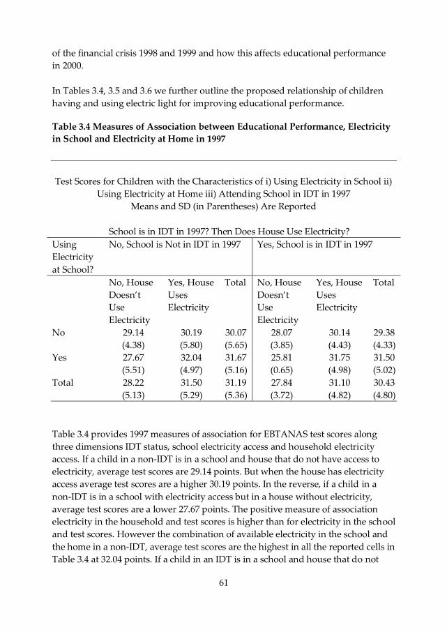
61

of the financial crisis 1998 and 1999 and how this affects educational performance

in 2000.

In Tables 3.4, 3.5 and 3.6 we further outline the proposed relationship of children

having and using electric light for improving educational performance.

Table 3.4 Measures of Association between Educational Performance, Electricity

in School and Electricity at Home in 1997

Test Scores for Children with the Characteristics of i) Using Electricity in School ii)

Using Electricity at Home iii) Attending School in IDT in 1997

Means and SD (in Parentheses) Are Reported

School is in IDT in 1997? Then Does House Use Electricity?

Using

Electricity

at School?

No, School is Not in IDT in 1997 Yes, School is in IDT in 1997

No, House

Doesn’t

Use

Electricity

Yes, House

Uses

Electricity

Total No, House

Doesn’t

Use

Electricity

Yes, House

Uses

Electricity

Total

No 29.14

(4.38)

30.19

(5.80)

30.07

(5.65)

28.07

(3.85)

30.14

(4.43)

29.38

(4.33)

Yes 27.67

(5.51)

32.04

(4.97)

31.67

(5.16)

25.81

(0.65)

31.75

(4.98)

31.50

(5.02)

Total 28.22

(5.13)

31.50

(5.29)

31.19

(5.36)

27.84

(3.72)

31.10

(4.82)

30.43

(4.80)

Table 3.4 provides 1997 measures of association for EBTANAS test scores along

three dimensions IDT status, school electricity access and household electricity

access. If a child in a non-IDT is in a school and house that do not have access to

electricity, average test scores are 29.14 points. But when the house has electricity

access average test scores are a higher 30.19 points. In the reverse, if a child in a

non-IDT is in a school with electricity access but in a house without electricity,

average test scores are a lower 27.67 points. The positive measure of association

electricity in the household and test scores is higher than for electricity in the school

and test scores. However the combination of available electricity in the school and

the home in a non-IDT, average test scores are the highest in all the reported cells in

Table 3.4 at 32.04 points. If a child in an IDT is in a school and house that do not

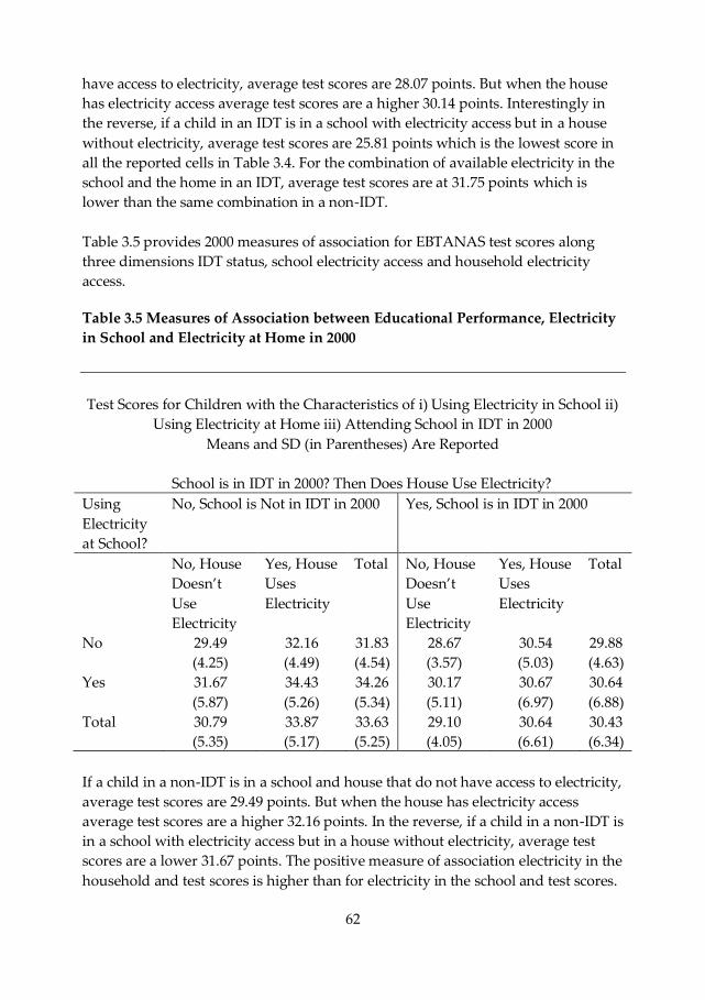
62

have access to electricity, average test scores are 28.07 points. But when the house

has electricity access average test scores are a higher 30.14 points. Interestingly in

the reverse, if a child in an IDT is in a school with electricity access but in a house

without electricity, average test scores are 25.81 points which is the lowest score in

all the reported cells in Table 3.4. For the combination of available electricity in the

school and the home in an IDT, average test scores are at 31.75 points which is

lower than the same combination in a non-IDT.

Table 3.5 provides 2000 measures of association for EBTANAS test scores along

three dimensions IDT status, school electricity access and household electricity

access.

Table 3.5 Measures of Association between Educational Performance, Electricity

in School and Electricity at Home in 2000

Test Scores for Children with the Characteristics of i) Using Electricity in School ii)

Using Electricity at Home iii) Attending School in IDT in 2000

Means and SD (in Parentheses) Are Reported

School is in IDT in 2000? Then Does House Use Electricity?

Using

Electricity

at School?

No, School is Not in IDT in 2000 Yes, School is in IDT in 2000

No, House

Doesn’t

Use

Electricity

Yes, House

Uses

Electricity

Total No, House

Doesn’t

Use

Electricity

Yes, House

Uses

Electricity

Total

No 29.49

(4.25)

32.16

(4.49)

31.83

(4.54)

28.67

(3.57)

30.54

(5.03)

29.88

(4.63)

Yes 31.67

(5.87)

34.43

(5.26)

34.26

(5.34)

30.17

(5.11)

30.67

(6.97)

30.64

(6.88)

Total 30.79

(5.35)

33.87

(5.17)

33.63

(5.25)

29.10

(4.05)

30.64

(6.61)

30.43

(6.34)

If a child in a non-IDT is in a school and house that do not have access to electricity,

average test scores are 29.49 points. But when the house has electricity access

average test scores are a higher 32.16 points. In the reverse, if a child in a non-IDT is

in a school with electricity access but in a house without electricity, average test

scores are a lower 31.67 points. The positive measure of association electricity in the

household and test scores is higher than for electricity in the school and test scores.

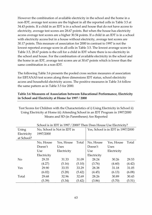
63

However the combination of available electricity in the school and the home in a

non-IDT, average test scores are the highest in all the reported cells in Table 3.5 at

34.43 points. If a child in an IDT is in a school and house that do not have access to

electricity, average test scores are 28.67 points. But when the house has electricity

access average test scores are a higher 30.54 points. If a child in an IDT is in a school

with electricity access but in a house without electricity, average test scores are

30.17 points. This measure of association for 2000 in contrast to 1997 is not the

lowest reported average score in all cells in Table 3.5. The lowest average score in

Table 3.5, 28.67 points is the cell for a child in IDT where there is no electricity in

the school and house. For the combination of available electricity in the school and

the home in an IDT, average test scores are at 30.67 points which is lower than the

same combination in a non-IDT.

The following Table 3.6 presents the pooled cross section measures of association

for EBTANAS test scores along three dimensions IDT status, school electricity

access and household electricity access. The positive measures in Table 3.6 follow

the same pattern as in Table 3.5 for 2000.

Table 3.6 Measures of Association between Educational Performance, Electricity

in School and Electricity at Home for 1997 / 2000

Test Scores for Children with the Characteristics of i) Using Electricity in School ii)

Using Electricity at Home iii) Attending School in an IDT Program in 1997/2000

Means and SD (in Parentheses) Are Reported

School is in IDT in 1997 / 2000? Then Does House Use Electricity?

Using

Electricity

at School?

No, School is Not in IDT in

1997/2000

Yes, School is in IDT in 1997/2000

No, House

Doesn’t

Use

Electricity

Yes, House

Uses

Electricity

Total No, House

Doesn’t

Use

Electricity

Yes, House

Uses

Electricity

Total

No 29.35

(4.27)

31.33

(5.16)

31.09

(5.10)

28.24

(3.76)

30.26

(4.60)

29.53

(4.42)

Yes 29.90

(6.02)

33.55

(5.28)

33.29

(5.42)

28.38

(4.45)

31.18

(6.13)

31.05

(6.08)

Total 29.68

(5.39)

32.96

(5.34)

32.69

(5.42)

28.26

(3.86)

30.89

(5.70)

30.43

(5.51)

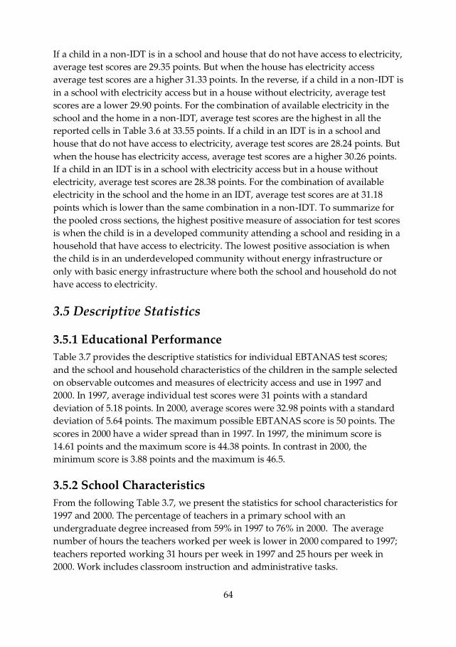
64

If a child in a non-IDT is in a school and house that do not have access to electricity,

average test scores are 29.35 points. But when the house has electricity access

average test scores are a higher 31.33 points. In the reverse, if a child in a non-IDT is

in a school with electricity access but in a house without electricity, average test

scores are a lower 29.90 points. For the combination of available electricity in the

school and the home in a non-IDT, average test scores are the highest in all the

reported cells in Table 3.6 at 33.55 points. If a child in an IDT is in a school and

house that do not have access to electricity, average test scores are 28.24 points. But

when the house has electricity access, average test scores are a higher 30.26 points.

If a child in an IDT is in a school with electricity access but in a house without

electricity, average test scores are 28.38 points. For the combination of available

electricity in the school and the home in an IDT, average test scores are at 31.18

points which is lower than the same combination in a non-IDT. To summarize for

the pooled cross sections, the highest positive measure of association for test scores

is when the child is in a developed community attending a school and residing in a

household that have access to electricity. The lowest positive association is when

the child is in an underdeveloped community without energy infrastructure or

only with basic energy infrastructure where both the school and household do not

have access to electricity.

3.5 Descriptive Statistics

3.5.1 Educational Performance

Table 3.7 provides the descriptive statistics for individual EBTANAS test scores;

and the school and household characteristics of the children in the sample selected

on observable outcomes and measures of electricity access and use in 1997 and

2000. In 1997, average individual test scores were 31 points with a standard

deviation of 5.18 points. In 2000, average scores were 32.98 points with a standard

deviation of 5.64 points. The maximum possible EBTANAS score is 50 points. The

scores in 2000 have a wider spread than in 1997. In 1997, the minimum score is

14.61 points and the maximum score is 44.38 points. In contrast in 2000, the

minimum score is 3.88 points and the maximum is 46.5.

3.5.2 School Characteristics

From the following Table 3.7, we present the statistics for school characteristics for

1997 and 2000. The percentage of teachers in a primary school with an

undergraduate degree increased from 59% in 1997 to 76% in 2000. The average

number of hours the teachers worked per week is lower in 2000 compared to 1997;

teachers reported working 31 hours per week in 1997 and 25 hours per week in

2000. Work includes classroom instruction and administrative tasks.

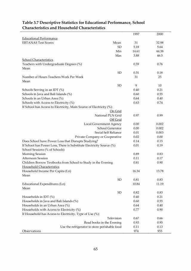
65

Table 3.7 Descriptive Statistics for Educational Performance, School

Characteristics and Household Characteristics

1997 2000

Educational Performance

EBTANAS Test Scores Mean 31 32.98

SD 5.18 5.64

Min 14.61 44.38

Max 3.88 46.5

School Characteristics

Teachers with Undergraduate Degrees (%)

Mean

0.59 0.76

SD 0.31 0.18

Number of Hours Teachers Work Per Week

Mean

31 25

SD 9 10

Schools Serving in an IDT (%) 0.40 0.21

Schools in Java and Bali Islands (%) 0.60 0.55

Schools in an Urban Area (%) 0.64 0.40

Schools with Access to Electricity (%) 0.63 0.74

If School has Access to Electricity, Main Source of Electricity (%):

On Grid

National PLN Grid 0.97 0.99

Off Grid

Local Government Agency 0.00 0.002

School Generator 0.00 0.002

Social Self Reliance 0.01 0.003

Private Company or Cooperative 0.02 0.00

Does School have Power Loss that Disrupts Studying? 0.14 0.15

If School has Power Loss, There is Substitute Electricity Source (%) 0.01 0.19

School Sessions (% of Schools)

Morning Session 0.89 0.83

Afternoon Session 0.11 0.17

Children Borrow Textbooks from School to Study in the Evening 0.81 0.90

Household Characteristics

Household Income Per Capita (Ln)

Mean

16.34 13.78

SD 0.81 0.83

Educational Expenditures (Ln)

Mean

10.84 11.19

SD 0.82 0.83

Households in IDT (%) 0.40 0.21

Households in Java and Bali Islands (%) 0.60 0.55

Households in an Urban Area (%) 0.64 0.40

Households with Access to Electricity (%) 0.77 0.90

If Household has Access to Electricity, Type of Use (%):

Television 0.67 0.66

Read books in the Evening 0.93 0.95

Use the refrigerator to store perishable food 0.11 0.13

Observations 974 955

66

Notes: Reported teacher hours worker per week consists of classroom instruction and administrative

tasks. For households with access to electricity, there are three possible types of use as asked by IFLS

(television, reading books in the evening and using the refrigerator to store perishable food). Each use is

separate from the other as IFLS does not ask if these uses overlap.

Based on the national curriculum, the number of teacher classroom instruction

hours should be 42 hours per week for fifth grade and sixth grade (our two grades

of interest in the specifications) but reported hours worked from Table 3.7 is lower.

The percentage of schools targeting children residing in an IDT is 40% in 1997 in

contrast to 21% in 2000. In the data we check that the children attend a school and

reside in a village within the boundaries of the same community classified as an

IDT. There is no incidence of a child for example attending a non-IDT designated

school while residing in an IDT.

Table 3.7 also provides statistics on the availability of electricity in schools. In 1997,

63% of schools observed report having electricity available. In 2000, 74% of schools

observed report electricity availability. For schools that have electricity, they also

report on the main source of electricity. In both 1997 and 2000, the main source of

electricity reported is the PLN grid; 97% of schools observed in 1997 and 99% of

schools observed in 2000. The remaining schools report other main sources of

electricity as the local government agency, school generator, social self reliance and

a private company or cooperative. In comparing school and household access to

electricity, in 1997, 63% of schools have electricity access compared to 77% of

households with electricity access. In 2000, the percentage of schools with

electricity access increases to 74% and there is also an increase to 90% in the

percentage of households being able to access electricity. In the IFLS questionnaire,

the schools are also asked if they lose electrical power which disrupts schooling. In

1997, 14% responded that there is power loss; in 2000 this response was 15%. A

subsequent IFLS question asked is when there is power loss the school has a

substitute electricity source available. In 1997, only 1% of schools observed

reported the availability of a substitute source but in 2000, an increased 19% of

schools have a substitute.

From IFLS, there is also information on start and end times for classroom sessions.

If schooling time is in the morning and afternoon, then natural sunlight is a

substitute for reading what is written on the blackboard, reading a book or writing

in class. However if an afternoon school session is running, classes end at 18:00h.

Natural sunlight ceases to be a substitute for electric light as the sun sets at 17:53h

in Western Indonesia and at 18:53h in Eastern Indonesia. In Table 3.7, schools

report that they offer two school sessions a day which maximizes the use of

classroom space. The two sessions are in the morning and in the afternoon. There

are no evening sessions.

67

In relation to how much learning material children can cover in the school day,

children can borrow Indonesian language and Math textbooks from the school.

Schools provide the children textbook loans for various reasons as documented in

IFLS – parents cannot afford to purchase the textbooks; parents can afford to

purchase the textbooks but the latest textbooks are not stocked in the local

bookstore; the school substitutes for the parents by purchasing and making

available the textbooks for use but the school budget is limited and children have to

share the textbooks during class time; and only a few children can access a

photocopier to make textbook copies. Because of these various reasons, in 1997 81%

of children borrow textbooks; and in 2000 this percentage increased to 90%.

3.5.3 Household Characteristics

Table 3.7 shows that average household income per capita in log terms for this

sample fell from 16.34 log points in 1997 to 13.78 log points in 2000. As detailed in

chapter 2, this is as a result of extreme price changes and depressed purchasing

power over the period of the financial crisis. The average deterioration in income

for this sample is larger than for the unrestricted sample in Chapter 2. In contrast

average household spending on education increased from 10.84 log points in 1997

to 11.19 log points in 2000. The percentage of households residing in an IDT is 40%

for 1997 and 21% in 2000. The percentage of all observed households that reside in

Java and Bali is 60% for 1997 and 55% for 2000. The percentage of households

residing in an urban area in 1997 is 64% and in 2000 it is 40%.

For household measures of electricity access and use, the percentage of households

that have access to electricity in 1997 is 77% and this rises to 90% in 2000. For

households that have access to electricity, the IFLS questionnaire asks if the

electricity is used for a television, a refrigerator to store perishable food or to read

books in the evening. The percentage of households that have electricity and use it

to watch television is 67% in 1997 and this percentage is 66% in 2000. In terms of

the use of light bulbs, the IFLS questionnaire asks if children bring home textbooks

from school to read in the evening. The percentage of children who responded

“Yes” to this question is 93% in 1997 and 95% in 2000. But there is no further

information on whether the children actually do read the textbooks that they bring

home from school.

3.6 Results

In Table 3.8 we present the output for specifications (i), (ii) and (iii) from Section

3.4. In column (1), using only the school characteristics base specification, the

percentage of undergraduate level qualified teachers and the facility for borrowing

school textbooks are positively related to EBTANAS test scores. Teacher quality

increases test score points by only 0.02 points and this is statistically significant at

68

the 1% level. Borrowing Indonesian language and Math textbooks from school

raises test scores by 0.25 points and this is statistically significant at the 5% level.

These very small gains to educational achievement compared to the other

explanatory variables can be seen across all specifications in columns (1) – (8). This

finding is then similar to what Bacalod and Tobias (2006) report that class size and

teacher training programs in Philippines’ primary schools matter less than

expected for test score performance.

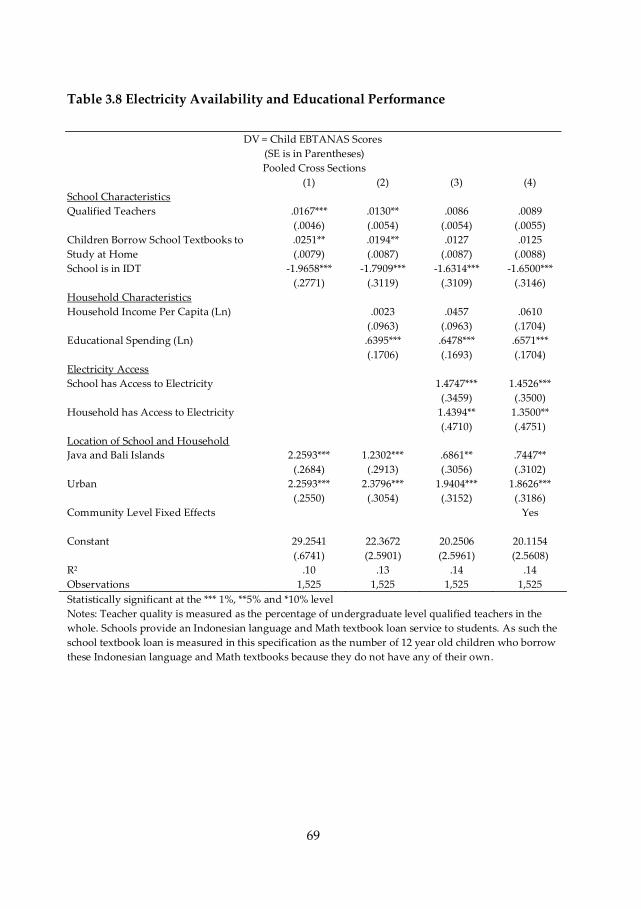
69

Table 3.8 Electricity Availability and Educational Performance

DV = Child EBTANAS Scores

(SE is in Parentheses)

Pooled Cross Sections

(1) (2) (3) (4)

School Characteristics

Qualified Teachers .0167***

(.0046)

.0130**

(.0054)

.0086

(.0054)

.0089

(.0055)

Children Borrow School Textbooks to

Study at Home

.0251**

(.0079)

.0194**

(.0087)

.0127

(.0087)

.0125

(.0088)

School is in IDT -1.9658***

(.2771)

-1.7909***

(.3119)

-1.6314***

(.3109)

-1.6500***

(.3146)

Household Characteristics

Household Income Per Capita (Ln) .0023

(.0963)

.0457

(.0963)

.0610

(.1704)

Educational Spending (Ln) .6395***

(.1706)

.6478***

(.1693)

.6571***

(.1704)

Electricity Access

School has Access to Electricity 1.4747***

(.3459)

1.4526***

(.3500)

Household has Access to Electricity 1.4394**

(.4710)

1.3500**

(.4751)

Location of School and Household

Java and Bali Islands 2.2593***

(.2684)

1.2302***

(.2913)

.6861**

(.3056)

.7447**

(.3102)

Urban 2.2593***

(.2550)

2.3796***

(.3054)

1.9404***

(.3152)

1.8626***

(.3186)

Community Level Fixed Effects Yes

Constant 29.2541

(.6741)

22.3672

(2.5901)

20.2506

(2.5961)

20.1154

(2.5608)

R2 .10 .13 .14 .14

Observations 1,525 1,525 1,525 1,525

Statistically significant at the *** 1%, **5% and *10% level

Notes: Teacher quality is measured as the percentage of undergraduate level qualified teachers in the

whole. Schools provide an Indonesian language and Math textbook loan service to students. As such the

school textbook loan is measured in this specification as the number of 12 year old children who borrow

these Indonesian language and Math textbooks because they do not have any of their own.

70

From Table 3.8, column (1) the negligible gains of teacher qualification and school

textbook loans are negated if the school is in an IDT where test scores drop by 2

points and this is statistically significant at the 1% level. The constant 0 is 29

points. If a child is in an IDT, the child has a lower starting score of 27 points

compared to a child in a developed area with 29 points. The result that a

disadvantaged child in an IDT school is in a lower starting position than a child

who is not in an IDT school is consistent across columns (1) – (4) in Table 8. This

suggests that a 12 year old child who attends school and resides in an IDT is in an

environment that negatively affects educational performance.

For the regional control variables, a child in Java and Bali Islands has a 1 point

advantage over a child in the other islands and a child in an urban area has a 2

point advantage over a child in a rural area. This implies that even if a child is in an

IDT and the IDT is in Java or Bali, instead of scoring 2 points less than a child in a

non-IDT, the performance gap is reduced to a 1 point difference. The estimate that

children in Java and Bali have better test scores than children in other islands,

holding other variables constant is seen across the specifications in columns (1) –

(8). But the size of the coefficient is reduced when household characteristics and

electricity access and use measures are included. This implies that children who

attend school and reside in Java and Bali have better educational performance

because school quality and the quality of the household environment including

access to electricity are higher in these islands compared to the other islands.

Similarly the estimate that children in urban areas have better test scores than

children in rural areas, holding other variables constant is seen across the

specifications in columns (1) – (8). However the coefficient size for urban areas

across the specifications is larger than the coefficient size for Java and Bali. This

may possibly suggest that within each of the main islands, when a child attends

school and resides in an urban area, this environment is conducive for schooling

and learning compared to a rural area.

In column (2), household characteristics are added to the specification. Household

income is positively related to test scores where a 1 log point change in income

shows a 0.002 change in test scores. But this estimate is not statistically significant.

A similar result is found across all specifications in columns (1) – (8). However

educational expenditures for the child show a positive relationship where a 1 log

point change in spending provides a 0.64 point change in test scores. This result is

statistically at the 1% level and is consistent across the specifications in columns (2)

– (4). This implies that family willingness to spend on education is far more

advantageous for a child’s education and this can be observed through educational

expenditures instead of family income. Also when taking into account in the

unpredictability of events of the Asian Financial Crisis in 1998, 1999 and to some

71

extent 2000, this result suggests that for this restricted sample reduced income has

less negative effect on outcomes than expected. The coefficients for school

characteristics have the same direction and magnitude in the second specification

as in the first specification. When viewing the influence of both the school and the

home on outcomes, it appears that the family has a more favorable role in

improving educational performance. This appears to be particularly the case when

the family is willing to set aside a proportion of available income specifically for

schooling expenditures. When considering that in this sample, families are less

inclined to migrate for schooling reasons, the family manages the existing quality

of schooling that they are confronted with by spending on different educational

expenditures that may improve performance e.g. private tuition, special courses,

writing supplies and different types of books.

In Table 3.8 columns (3) and (4), we now introduce measures of electricity

availability in the school and household. Community level fixed effects are

controlled for in column (4). The endogenous explanatory variables qualified

teachers and the school textbook loan lose statistical significance while the negative

relationship of an IDT school and test scores continues to hold and be statistically

significant at the 1% level. However the introduction of electricity access slightly

reduces the magnitude of the IDT school variable by 0.1 points. Of the two

measures of electricity access, school availability of electricity is related to slightly

higher test scores than household electricity availability. When the school has

access to electricity, test scores increase by 1.4 points and this is statistically

significant at the 1% level. When the home has access to electricity, test scores

increase by 1.4 points in column (3) and increase by 1.3 points when community

level fixed effects are added which can be seen in column (4). Both estimates are

statistically significant at the 1% level. Based on our empirical specification, the

availability of electricity has a time lagged effect on test scores. So the increase in

test scores is likely to be cumulative over the period of time the child has access to

electricity in school and the household. This implies that when the child is in an

environment where both the school and the home have continued access to

electricity, educational performance improves substantially. Since in this sample,

families do not move to communities that have better quality schools, by merely

having electrical connections in school and the household, children’s educational

performance can improve.

In Table 3.9 we present the output for specification (iv) from Section 3.4. This

expanded specification introduces measures of electricity use in the school and

household. While the use of electricity in school is for studying, families use

electricity at home for various work and leisure activities. These activities may

directly or indirectly influence learning over time. To examine the potential

pathways from electricity availability to electricity use in the household, Table 3.9

72

columns (5) and (6) provide estimates of the child who studies at home using

borrowed textbooks from school and the child who watches television at home.

Columns (7) and (8) sub-divide these activities by IDT to assess if within an

underdeveloped environment, unobserved factors will influence these two

activities differently compared to a developed community. For example, in an IDT

basic infrastructure provides lower access to electricity. Scholastically motivated

families may then choose to use the limited or rationed electricity by substituting

away from non-learning related activities to learning activities in favor of their

child’s development.

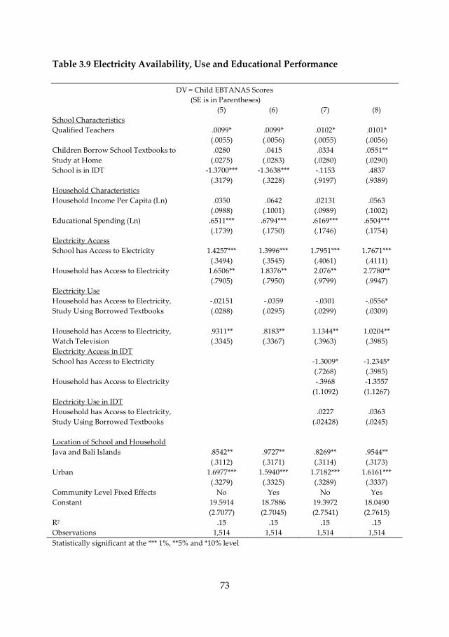
73

Table 3.9 Electricity Availability, Use and Educational Performance

DV = Child EBTANAS Scores

(SE is in Parentheses)

(5) (6) (7) (8)

School Characteristics

Qualified Teachers .0099*

(.0055)

.0099*

(.0056)

.0102*

(.0055)

.0101*

(.0056)

Children Borrow School Textbooks to

Study at Home

.0280

(.0275)

.0415

(.0283)

.0334

(.0280)

.0551**

(.0290)

School is in IDT -1.3700***

(.3179)

-1.3638***

(.3228)

-.1153

(.9197)

.4837

(.9389)

Household Characteristics

Household Income Per Capita (Ln) .0350

(.0988)

.0642

(.1001)

.02131

(.0989)

.0563

(.1002)

Educational Spending (Ln) .6511***

(.1739)

.6794***

(.1750)

.6169***

(.1746)

.6504***

(.1754)

Electricity Access

School has Access to Electricity 1.4257***

(.3494)

1.3996***

(.3545)

1.7951***

(.4061)

1.7671***

(.4111)

Household has Access to Electricity 1.6506**

(.7905)

1.8376**

(.7950)

2.076**

(.9799)

2.7780**

(.9947)

Electricity Use

Household has Access to Electricity,

Study Using Borrowed Textbooks

-.02151

(.0288)

-.0359

(.0295)

-.0301

(.0299)

-.0556*

(.0309)

Household has Access to Electricity,

Watch Television

.9311**

(.3345)

.8183**

(.3367)

1.1344**

(.3963)

1.0204**

(.3985)

Electricity Access in IDT

School has Access to Electricity -1.3009*

(.7268)

-1.2345*

(.3985)

Household has Access to Electricity -.3968

(1.1092)

-1.3557

(1.1267)

Electricity Use in IDT

Household has Access to Electricity,

Study Using Borrowed Textbooks

.0227

(.02428)

.0363

(.0245)

Location of School and Household

Java and Bali Islands .8542**

(.3112)

.9727**

(.3171)

.8269**

(.3114)

.9544**

(.3173)

Urban 1.6977***

(.3279)

1.5940***

(.3325)

1.7182***

(.3289)

1.6161***

(.3337)

Community Level Fixed Effects No Yes No Yes

Constant 19.5914

(2.7077)

18.7886

(2.7045)

19.3972

(2.7541)

18.0490

(2.7615)

R2 .15 .15 .15 .15

Observations 1,514 1,514 1,514 1,514

Statistically significant at the *** 1%, **5% and *10% level

74

Notes: Teacher quality is measured as the percentage of undergraduate level qualified teachers in the

whole. Schools provide an Indonesian language and Math textbook loan service to students. As such the

school textbook loan is measured in this specification as the number of 12 year old children who borrow

these Indonesian language and Math textbooks because they do not have any of their own.

In Table 3.9 columns (5) – (8), household access to electricity now provides larger

estimates for test score performance compared to school access to electricity. When

the home has electricity access scores increase by 1.65 points (column (5)) and 1.83

points (column (6)). Column (6) includes community level fixed effects. In contrast,

when the school has electricity access scores increase by 1.42 points (column (5))

and 1.39 points (column (6)). All four estimates are statistically significant. This

result appears to be the case because of the introduction of the variables

representing the type of use for electricity at home. When the household has access

to electricity and this variable interacts with the number of children who borrow

school Indonesian language and Math textbooks to read at home, test scores are at

a lower 0.02 points in column (5) and a lower 0.03 points in column (6). But these

results are statistically insignificant. This may suggest the children are less likely to

read their Indonesian language and Math textbooks in the evening. Instead they

may prefer to read other textbooks that their parents have purchased such as

science, social studies and religious studies. Children from Muslim households and

who attend MORA religious schools may prefer to recite the Koran. Or they may

prefer to read other types of books, comics and newspapers, all of which can

positively influence their cognitive skills. More interestingly, in columns (5) and (6)

when the household has access to electricity and this interacts with the variable for

whether the child watches television, test scores increase by 0.93 points. With a

control for community fixed effects, scores increase by 0.81 points. Both results are

statistically significant at the 5% level. A possible interpretation is that when the

child is able to watch television after school, the child watches programs with

educational content such as the Indonesian television channel Television Pendidikan

Indonesia (TPI or Education Television Indonesia). Or the child is able to watch

general programs on television that improve his or her language skills. Our

findings are similar to Gentzkow and Shapiro (2008) who use the American

Coleman Study data to show that younger children with an additional year of

television exposure have higher reading and verbal test scores when they are older.

In Table 3.9 columns (7) and (8), we study more in-depth the access and use of

electricity in the household by IDT status. Without controls for community level

fixed effects, if the child is in an IDT school, test scores fall by 0.11 points. But

unexpectedly, with fixed effects a child in an IDT school now has an increase in test

scores by 0.48 points. While these results are not statistically significant, they may

be of education significance. This may be of significance because despite

disadvantages faced in a community, families in such a community still have a

high preference for their children to have high educational achievement. The

75

magnitude of the IDT school coefficient in these two specifications is much smaller

than the specifications in columns (1) – (6). This is because of the introduction of

electricity access and use in IDT communities. When children attend an IDT school

that has access to electricity, test scores fall by 1.3 points (column (7)) and with

fixed effects fall by 1.2 points (column (8)). Both estimates are statistically

significant at the 10% level. In comparison, all children without conditioning on

IDT, access to electricity in school and test score performance is positive at 1.7

points and statistically significant at the 1% level. Similarly children are in IDT

households that have access to electricity, test scores fall by 0.4 points and with

community level fixed effects scores fall by 1.3 points. But these estimates are not

statistically significant. A possible interpretation is that in an IDT community,

schools and households have only basic infrastructure and electricity access may be

capturing the negative effect of underdevelopment on children’s performance. IDT

underdevelopment where there is poverty, a lack of employment opportunity and

a lack of public services including quality schooling may perhaps be viewed as a

source of disadvantage for children.

From Table 3.9, when we assess the use of electricity by IDT status, interestingly we

find that in an IDT household with electricity and children study using borrowed

Indonesian language and Math textbooks, test scores increase by 0.02 points. With

community level fixed effects scores increase by 0.03 points. In contrast, the

association for these two variables is negative for all children who have electricity

available for reading textbooks. This may imply that given the disadvantaged

position that children have in education in IDT communities, the mere opportunity

to borrow school textbooks and to be able to have electricity at home to read these

textbooks may motivate them to study. However the coefficient for the interaction

between household access to electricity and watching television has a negative sign

for children in IDT and is statistically insignificant. This is as opposed to all

children who watch television. Possible reasoning for this negative relationship is

IDT households while able to watch television may not have a reliable signal

reception since they may be located in a remote area. In the literature, Olken (2009)

finds that the variation in television signal reception and strength in Java Island

affects how many hours a day that Indonesians can watch television. If this is the

case for children in IDT households, they may be less likely able to watch

educational programs (e.g. the TPI channel). As such the television variable in the

specification may not be able to capture the positive effect on test scores.

In reconciling the estimates for IDT school status and the use of electricity in an IDT

household, the specification in column (8) with community level fixed effects raises

an interesting observation. In this specification, the negative relationship between a

child attending an IDT school and educational performance reverses and becomes

positive. The possible pathway from basic infrastructure that introduces access

76

(albeit low access) to electricity in an IDT community may lead to parents

preferring to let their children use the limited electricity available for studying in

the evening. This implies that low income families from underdeveloped areas may

demonstrate a preference for education if the physical environment is conducive

for them to choose learning for their children instead of other activities.

3.7 Conclusions In this chapter we have investigated if there is a relationship between the

availability and use of electricity and the educational performance of 12 year old

Indonesian children in primary school. Using EBTANAS test scores which capture

the child’s historical performance from grade 1 to grade 6 of primary school we

find that for 1997 and 2000, the availability of electricity in school and the

household raises test scores substantially and these results are statistically

significant. In establishing a potential pathway between electricity availability and

test scores, we find that how families use electricity in the household influences

outcomes. When children watch television at home, test scores markedly increase

after controlling for community level fixed effects. This may perhaps be attributed

to educational programming on national television. Conditioning on attending

school in an underdeveloped, below the poverty line, left behind village (IDT)

children who borrow school textbooks to study at home in the evening have

slightly improved test scores. While households use electricity for various reasons,

there is evidence that there are families who choose to use electricity for activities

where their children can learn better. This may be particularly the case for families

in underdeveloped areas where they are constrained in electricity access because of

rationing by the state.

Over the period of 1997 and 2000, more schools and households in our sample are

connected to the national PLN grid as well as off the grid to access electricity.

Particularly there are a higher proportion of households than schools that have

access to electricity. Studying and doing homework in the evening most likely

complement what the child learns in the classroom in the day. By having access to

electricity in the child’s daily environment both in school and at home, it is very

likely that the child is more motivated to learn and complete primary school. This

is regardless of a disadvantaged background such as the child coming from an

underdeveloped community or regardless of volatilities faced by the family during

the Asian Financial Crisis. However given the fixed placement of the national PLN

grid, where over 70% of energy is allocated for industrial use (industrial sector and

transport sector) and where Java and Bali receive 77% of total energy capacity, not

all communities are able to receive full access to electricity. Also children who

attend school and reside in urban areas tend to have more access to electricity and

better educational outcomes. This strongly implies that access to electricity is a

77

potential resource constraint on children’s educational outcomes. This is unless

families move from areas that have low access to electricity to areas with high

access to electricity in order to ensure that their children have a favorable learning

environment. However using available data, we are unable to conclude whether a

family’s out-migration for schooling reasons in Indonesia will improve outcomes.

On the basis of these results, the supply and provision of electricity to the

communities of the Outer Islands - Sumatera, Kalimantan, Sulawesi and Nusa

Tenggara is a concern. The public policy issue then is about the distribution of

energy for final use to all islands and not just the availability of energy. The

distribution of energy should cover all parts of an island and not just the urban

areas that have more waged economic activity. By considering that electricity

access promotes an environment that is conducive for schooling more children will

be motivated to pass their achievement tests at the primary school level. Then they

are more likely to progress on to junior high. But until then, the lack of access to

electricity in certain regions of Indonesia is a constraint on educational

achievement.

78

4. Household Income, Simultaneous Work-

Schooling and Human Capital

79

4.1 Introduction

This chapter studies the phenomenon of joint child work-schooling decisions in

Indonesia from the view of human capital theory. Productive skills are developed

in childhood for generating future returns. Human capital can be accumulated not

just by attending formal schooling but also through informal schooling such as

learning skills from the family. In Indonesia the national labor force starts at age 10

and this consists of economically active children who have either never attended

school or who combine work with schooling. For children who are in the labor

force while simultaneously attending school, this raises the question as to the

extent that the child’s labor supply affects the amount of time available to develop

skills. To address this, consideration has to be given to the timing of schooling,

whether this timing conflicts with work and the extent of this conflict. If there is

conflict this arises from the joint work-schooling decision that is influenced by

whether the child’s income augments household income and possibly the social

norms towards children working.

This chapter studies Indonesian child workers aged 6 – 15 who simultaneously

attend school. Two questions are asked. Does a reduction in parental income

change simultaneous work-schooling behavior? If yes, do these changes impair

human capital accumulation? In this chapter, I view child labor in terms of

economic work and unpaid household production / domestic work and I use the

terms schooling and skill formation interchangeably. I sequence the behavior of

simultaneous work-schooling as a child who first works and then second attends

school. As child labor and school decisions are joint outcomes out of a single time

allocation problem, I analyze the joint decision-making by studying the children’s

types of work and learning activities in and outside of the household and time

allocated to these activities. Using the Indonesian education system which

recognizes the phenomenon of child labor and provides skill development

alternatives for child workers18, I study three sources of skill formation. The first is

the formal and mainstream system of primary school and junior high. The second

is non-formal school which consists of alternatives to the mainstream system that

target child workers (refer to Chapter 2 for a full description of these three sources

of skill formation and how they are structured with the education system).

Educational service delivery for non-formal schooling includes the use of privately

managed religious schools; learning time is flexibly built around the child’s

working time. The third is informal school which consists of the provision of

independent study modules to complement the skills acquired from education

18 The previous chapters were related to the formal and mainstream education system. This chapter

expands on the system to examine alternative schooling for child workers.

80

within the home. Households that typically have informal schooling are parents

who are traders or entrepreneurs and have children who act as apprentices. Apart

from skill development, children who work in the household should face fewer

safety and health risks compared to children working outside without parental

supervision or monitoring.

In the literature on household income and child labor, Basu, Das, and Dutta (2007)

provide a discussion on child labor responses to variations in household income.

These responses include whether the child shifts from work within the household

to work outside the household. Work within the household is more likely if the

household has its own business as discussed by Edmonds and Turk (2004) for

Vietnamese households. In the overwhelming majority of cases, the work

performed by children takes place within the household – usually household

chores and work on the family farm (Basu and Ray, 2002). Wage work and work in

small enterprises which take place outside the household remains an exception

(ILO, 2002). The UNICEF definition of child labor reflects the distinction made

between working outside and in the household as well as recognizing that the

intensity of child labor is higher when the child is older19. In Asia, a further

distinction is made where child labor is primarily regarded as an urban as opposed

to rural phenomenon (Fafchamps and Wahba, 2006). However it is unclear whether

the activities carried out in the household necessarily constitute child labor if the

child is an apprentice in the family enterprise, building skills through on-the-job

learning. Given the state of the literature, my contribution is to produce more

insight on how joint work-schooling does not impair human capital accumulation.

The rest of the chapter is organized in the following way. In Section 4.2 I describe

national level trends of child labor in Indonesia and how this changed over the

period of the financial crisis. Section 4.3 describes the natural experiment and a

description of the dataset, the RAND Corporation Indonesia Family Life Surveys

(IFLS). Limitations arising from the observed data i.e. child labor as the dependent

variable is a censored variable (Basu et al, 2007) are discussed. Section 4.4 details

the child and household characteristics associated with work-schooling behavior

which I use for the estimations. Section 4.5 reports the results. Conclusions are in

Section 4.6.

19 UNICEF definition of child labor: children aged 5 – 11 who work at least 1 hour of economic work or

28 hours of domestic work per week; children aged 12 – 14 who work at least 14 hours of economic

work or 28 hours of domestic work per week.

81

4.2 National Child Labor and Schooling Trends The Asian Financial Crisis (AFC) occurred at the end of 1997 with effects in the

financial markets felt until the beginning of 2000. For the household, much of the

impact of the aggregate shock was felt in the 52.16 percentage point or eightfold

increase in inflation rates from 1997 to 1998. With reference to Chapter 2 Table 2.1,

annual inflation rates increased from 6.23% in 1997 to 58.39% in 1998 and then

improving to 20.49% in 1999 before resuming a considerably lower rate of 3.72% in

2000. Inflation rates were then less substantial in 1999. The significant increases in

inflation rates for the two years 1998 and 1999 compared to 1997 and 2000 severely

weakened household purchasing power of all goods including education.

In terms of schooling indicators, between 1997 and 199820 the percentage of 13-19

year olds that were not currently enrolled in school rose. The percentage not

enrolled increased more in urban centers - from 33 percent in 1997 to 38 percent in

1998, a change that is statistically significant. Children from poorer households in

general were more likely not to be enrolled in school compared to children from

higher income households — a phenomenon that intensified between 1997 and

1998. Younger children were less likely to be in school in 1998 as well. This is

especially true for the poorest. The percentage of 7 - 12 year olds in the bottom

quartile of the distribution of per capita expenditure that were not enrolled

implying delayed starting in school doubled, from about 6% in 1997 to about 12%

in 1998. But based on an empirical investigation carried out by Cameron (2001) in

Indonesia declines in schooling do not appear to be accompanied by a rise in

formal employment amongst children.

In terms of the occurrence of child labor, the Indonesian Census Bureau of

Statistics, BPS national labor force surveys SAKERNAS show that at least 1% of

children starting from age 5 to 9 are economically active (SAKERNAS 1998; Asra et

al 1995 and 1997). However detailed information is not available for this age group.

Using SAKERNAS, available data shows that the percentage and absolute number

of economically active children in Indonesia becomes noticeable when the child is

aged 10 onwards. With reference to Figure 4.1, it can be seen that there is a trend

where there are children who simultaneously work and attend school.

20 World Bank Indonesia Statistics

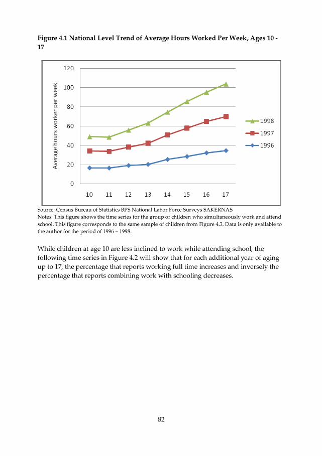
82

Figure 4.1 National Level Trend of Average Hours Worked Per Week, Ages 10 -

17

Source: Census Bureau of Statistics BPS National Labor Force Surveys SAKERNAS

Notes: This figure shows the time series for the group of children who simultaneously work and attend

school. This figure corresponds to the same sample of children from Figure 4.3. Data is only available to

the author for the period of 1996 – 1998.

While children at age 10 are less inclined to work while attending school, the

following time series in Figure 4.2 will show that for each additional year of aging

up to 17, the percentage that reports working full time increases and inversely the

percentage that reports combining work with schooling decreases.

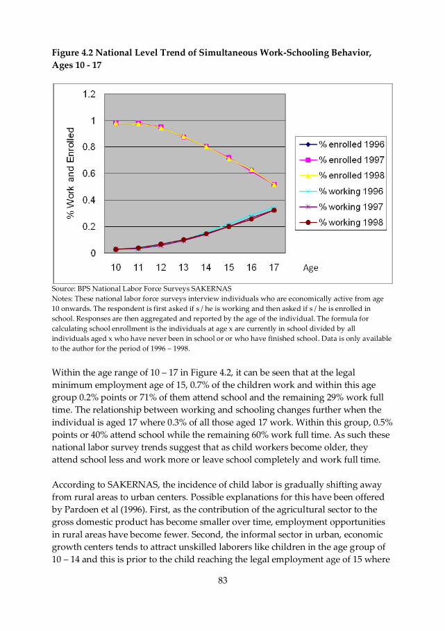
83

Figure 4.2 National Level Trend of Simultaneous Work-Schooling Behavior,

Ages 10 - 17

Source: BPS National Labor Force Surveys SAKERNAS

Notes: These national labor force surveys interview individuals who are economically active from age

10 onwards. The respondent is first asked if s / he is working and then asked if s / he is enrolled in

school. Responses are then aggregated and reported by the age of the individual. The formula for

calculating school enrollment is the individuals at age x are currently in school divided by all

individuals aged x who have never been in school or or who have finished school. Data is only available

to the author for the period of 1996 – 1998.

Within the age range of 10 – 17 in Figure 4.2, it can be seen that at the legal

minimum employment age of 15, 0.7% of the children work and within this age

group 0.2% points or 71% of them attend school and the remaining 29% work full

time. The relationship between working and schooling changes further when the

individual is aged 17 where 0.3% of all those aged 17 work. Within this group, 0.5%

points or 40% attend school while the remaining 60% work full time. As such these

national labor survey trends suggest that as child workers become older, they

attend school less and work more or leave school completely and work full time.

According to SAKERNAS, the incidence of child labor is gradually shifting away

from rural areas to urban centers. Possible explanations for this have been offered

by Pardoen et al (1996). First, as the contribution of the agricultural sector to the

gross domestic product has become smaller over time, employment opportunities

in rural areas have become fewer. Second, the informal sector in urban, economic

growth centers tends to attract unskilled laborers like children in the age group of

10 – 14 and this is prior to the child reaching the legal employment age of 15 where

84

labor laws can afford protection to the child. Also when comparing urban

employment with rural employment opportunities, it has been reported that the

urban informal sector provides higher and more stable incomes for child workers.

Particularly over the period of the financial crisis, Imawan (1999) documented that

in urban centers the number of working children rose from 1% to 1.5% in the

period of August 1997 to December 1998. Although the majority of the children

observed in this period still worked in the agricultural sector (64.4%), it is reported

that 14.7% worked in the manufacturing sector and 20.9% worked in the services

sector which includes street children who will provide services for a fee (BPS,

1998).

The gradual shift from the primary (agricultural) sector to secondary

(manufacturing) and tertiary (services) sectors has also gradually reduced the

number who work for less than 24 hours a week (Pardoen et al, 1996). This is

associated with children shifting from non-wage employment to wage

employment. Non-wage employment tends to occur when the child is engaged in

work in the household such as family farm production or home production /

domestic work. As a result, their working status as classified by BPS and

SAKERNAS as changing from unpaid family workers to laborers is when they shift

from non-wage employment to wage employment. With reference to the publicly

available BPS household survey SUSENAS 2000 as detailed in Table 4.2, the

working status of children can be defined as being i) self employed without family

assistance ii) self-employed with family assistance iii) self-employed with non-

family assistance iv) paid worker and v) unpaid worker in the family. For

definitions i) to iii), the child worker may or may not receive a wage.

85

Table 4.1 Working Status of Children by Urban / Rural and Gender

(% and Count is in Parentheses)

Urban Rural Girl Boy

Self-employed without

family assistance (paid and

unpaid)

9.4 (63) 5.7 (287) 5.0 (107) 6.8 (243)

Self-employed with family

assistance (paid and unpaid)

3.9 (26) 4.0 (202) 3.6 (77) 4.2 (151)

Self-employed with non-

family assistance (paid and

unpaid)

0.3 (2) 0.2 (8) 0.6 (6) 0.4 (4)

Paid worker 32.1 (216) 7.5 (375) 12.3 (265) 9.2 (326)

Unpaid worker in the family 54.5 (366) 82.7 (4,160) 78.8 (1,693) 79.6 (2833)

Total 100 (673) 100 (5,032) 100 (2,143) 100 (2,889) Source: BPS Household Survey SUSENAS 2000.

Notes: Given restrictions on accessing data, this is the only nationally representative sample publicly

available on child labor.

From Table 4.1, definitions i) and ii) when contrasted against iii) suggests that the

child worker may face higher safety and health risks without the presence of the

family. From this table too, it appears that the vast majority of child workers are

unpaid workers in the family located in rural areas. Also both female and male

child workers tend to be unpaid workers in the family.

The labor surveys also show that the proportion of male children who are

economically active has tended to rise over time (SAKERNAS 1998 – 1993, Pardoen

et al, 1996). However, according to Irwanto et al (2001) the national level trends

may be under-reporting the incidence of girls working. This is because they tend to

engage in home production / domestic production for the family and are not

remunerated.

86

4.3 Empirical Strategy

My research design is a natural experiment where I exploit the timing of the RAND

Corporation Indonesia Family Life Surveys (IFLS) wave 2 (1997) and wave 3 (2000)

to identify an exogenous source of variation in income - the Asian Financial Crisis.

This instrument enables me to study the variations to simultaneous work-schooling

behavior.

I define child work as i) a child aged 6 – 15 who works outside the household and

may or may not receive a wage and ii) a child aged 6 – 15 who works in the

household and does not receive a wage. I define schooling in terms of the three

sources of skill formation – formal, non-formal and informal. I have the two

definitions for work outside and in the household which follows from the

analytical model by Edmonds (2008) and the generalized child labor model by

Cigno and Rosati (2005). Both models imply that for most children the return to

time for work in the household (household production) is at least as large as the

value the family places on the child’s wage contribution from working outside the

household. These two labor definitions are also operationally similar to the

UNICEF definition of child labor and the information that I have concerning the

work status of children as defined in Table 4.2 particularly that the vast majority of

children are unpaid workers in the household. Work activities in the household

include participating in the family enterprise, farming, home production and

domestic work. I only consider the age range of 6 – 15 because children in the

formal education system start basic education either at end of age 6 or beginning

age 7 and complete their education at the end of age 14. Starting age 15, the child

can legally enter the labor market.

There are 3 different specifications for the dependent variable, child labor for its

response to a reduction in household income. This is because I would like to

capture different dimensions of child labor to prevent understating the magnitude

of child labor. Also these specifications enable me to study the dynamics of child

time allocation between work and learning activity. Using these specifications, I

explore i) the changes to the shift between work activity and schooling activity, ii)

changes between working outside the household and within the household; and iii)

if the child works outside the household, changes to the number of hours worked

per week. I match the children in the 1997 wave and the 2000 wave using the same

household characteristics, child characteristics and schooling type / source of skill

formation. These characteristics and how they relate to my two research questions

are detailed in Section 4.4. Only biological parent – child relationships are

considered. The estimates for child labor are then specified in the following

reduced form:

87

ittiititit fscmy 43210 <(1)

where icy is the dependent variable with three different specifications for work by

child i

i) if child works and attends school then 1 and if child has no work and attends

school full time then 0,

ii) if child works outside the household and attends schools then 1 but if child

works in the household and attends school then 0 and

iii) if child works outside the household and attends school, the number of hours

worked per week; itm represents household characteristics that vary before and

after the financial crisis – income and educational expenditures; itc captures child

characteristics over time t; is is a dummy variable that represents each of the three

schooling types / sources of skill formation and tf is a dummy variable for the

financial crisis.

Since I can only observe child and household behavior in 1997 and 2000, it is

acknowledged that I cannot observe anything spread across 1998 and 1999 given

data unavailability; this is where there is severe unpredictability in behavior.

Consequently, I carry out instrumental variable estimation to isolate the

relationship between parental income and simultaneous work-schooling behavior.

The IV approach is used to manage the omitted variable bias problem that is faced

from not being able to observe child and household behavior over the period of

1998 and 1999 as well as to enable a discussion of alternative explanations for

variations in child labor. As the instrument I use is the financial crisis, this

instrument works through the value of child time where the variation in child labor

is owing to the family’s need for the child’s contribution to household income or

the relative return to work rather than school. This is written as equation (2) where

the endogenous explanatory variable income mit is a linear function of the

exogenous variable the AFC z4, a dummy variable and an error term.

itit zzzzm 443322110 <(2)

I run OLS and IV regressions using the three different specifications for the

dependent variable. An alternative method considered would have been a

multinomial logit (MNL). But I do not choose this alternative because I am unable

to determine or order the hierarchy of choices for MNL. In the first restricted

sample, the dependent variable consists of both children who combine work with

school or who combine zero work with school full time. In the second restricted

sample, the dependent variable consists of both children who work outside the

household or in the household and gain a skill from one of the schooling types –

88

formal, non-formal and informal. Children who attend school full time are not

included in this second restricted sample. The size for the second sample is larger

than for the first sample because in the data there are more children who

demonstrate the behavior of work combined with schooling compared to children

attend school full time. In the third restricted sample, I then proceed to focus only

on children who work outside the household who report the number of hours

worked while simultaneously attending one of the school types. This is because in

IFLS waves 2 and 3 only children who work outside the household report the

number of hours worked. The sample size becomes substantially smaller which

then inevitably reduces the power of the analysis. However by comparing the

direction and magnitude of the relationship between the main variables of interest

using all 3 samples, I will have more information for analysis and interpretation.

A limitation of IFLS which is unavoidable and I account for this in my empirical

strategy is the possibility of household break-up in longitudinal study designs. This

limitation arguably cannot simply be explained away in terms of attrition. As

explained by Rosenzweig and Foster (2001) this design problem stems in part from

the relative absence of attention in the theoretical and empirical literature to the

determination of household structure. I try to address this problem by looking at

the data in terms of household splitting. That is, there may be children who out-

migrate for employment reasons. But none of the children aged 6 – 15 report

leaving the household to start a new household in another location.

4.4 Child and Household Characteristics in Simultaneous

Work-Schooling Behavior

The allocation of child time is an important component of a household's decision-

making process. The household must weigh the value of child time spent in many

activities including schooling, wage work, work inside the household, and work in

household chores or other components of household production. The value of child

time in any of these activities depends on both child and household attributes. In

this section I consider how observable child and household characteristics are

associated with the degree to which household income is improved over the period

of the financial crisis. To do this I carry out semi-parametric estimation and I

assume a normal distribution.

To capture child characteristics I use the variables gender, age and schooling type

or source of skill formation. But there is a limitation where there is no data

available on the type of work activity that the child carries out outside the

household or in the household. As detailed in Section 4.3, these are the

characteristics that are associated with the value of child time. National level trends

89

show that boys tend to work outside the household and this work can be waged or

non-waged. Wage work can be valued in terms of hourly wages or a fixed wage for

a given amount of work. In contrast girls tend to work in the household or also

known as attending informal school, primarily in farming, home production or

domestic work which is unremunerated. It is then difficult to monetize the value of

their work and how it improves family welfare. It is also difficult to measure the

number of hours girls allocate to work because there is no incentive to determine

the monetary value of an hour’s work. Because of these intrinsic differences in how

the work effort of boys and girls are viewed, there will also be differences in terms

of how boys and girls shift more towards work and less towards schooling given

joint work-schooling decisions. I capture these differences using the two definitions

of child work – work outside the household and work in the household.

In terms of household characteristics, I focus on the variables annual total

household income and household educational expenditures. Household income is

proxied by household reported expenditures on all market valued goods and

services. Educational expenditures consist of spending in the whole school year

related to learning activity such as books, private tuition and transportation to

school or the learning center. Because of the unanticipated reduction in household

income, adjustments to household expenditures may necessitate reducing or

foregoing educational expenditures entirely. However scholastically motivated

parents may likely continue to allocate a proportion of the household budget to

learning activity.

In relation to child and household attributes, I consider too the regional differences.

This is because of the vastness of the country and its different socio-economic

characteristics. To capture the regional differences, I use two variables – all

households residing in Java and Bali Islands and households split by urban and

rural in each of the main islands. Because of modernization and consequently

urbanization, Java and Bali Islands have attracted the majority of the population.

Java and Bali based on BPS estimates in 2003 are home to 60% of the total country

population but represent only 7% of the total land mass in Indonesia. In contrast

the Outer Islands are considered to have less industrialization, are less developed

and have a lower population density.

4.4.1 Distribution of Time for Work and Schooling

I present the distribution of hours worked per week while attending school and

one of the sources of skill formation. The kernel densities to be presented in Figures

4.3, 4.4 and 4.5 represent child work outside of the household but not child work in

the household. Based on the survey question asked in IFLS, children report on

actual number of hours worked in the previous week and the hours reported do

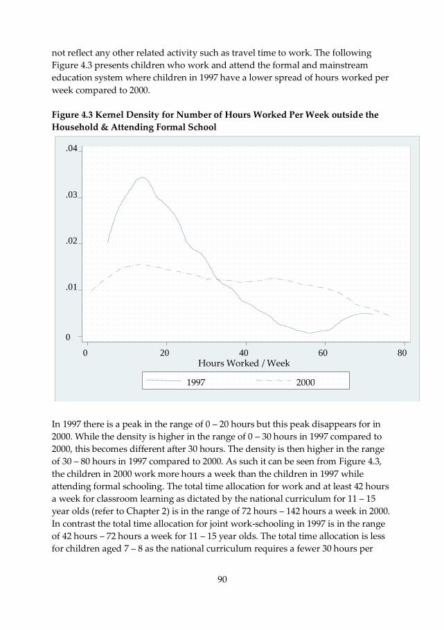
90

not reflect any other related activity such as travel time to work. The following

Figure 4.3 presents children who work and attend the formal and mainstream

education system where children in 1997 have a lower spread of hours worked per

week compared to 2000.

Figure 4.3 Kernel Density for Number of Hours Worked Per Week outside the

Household & Attending Formal School

In 1997 there is a peak in the range of 0 – 20 hours but this peak disappears for in

2000. While the density is higher in the range of 0 – 30 hours in 1997 compared to

2000, this becomes different after 30 hours. The density is then higher in the range

of 30 – 80 hours in 1997 compared to 2000. As such it can be seen from Figure 4.3,

the children in 2000 work more hours a week than the children in 1997 while

attending formal schooling. The total time allocation for work and at least 42 hours

a week for classroom learning as dictated by the national curriculum for 11 – 15

year olds (refer to Chapter 2) is in the range of 72 hours – 142 hours a week in 2000.

In contrast the total time allocation for joint work-schooling in 1997 is in the range

of 42 hours – 72 hours a week for 11 – 15 year olds. The total time allocation is less

for children aged 7 – 8 as the national curriculum requires a fewer 30 hours per

0

.01

.02

.03

.04

0 20 40 60 80 Hours Worked / Week

1997 2000

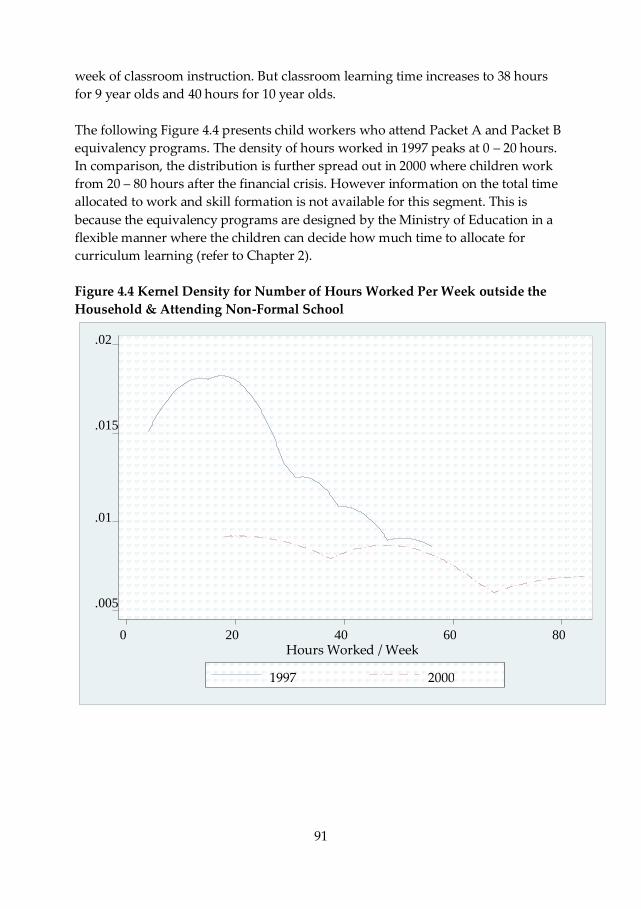
91

week of classroom instruction. But classroom learning time increases to 38 hours

for 9 year olds and 40 hours for 10 year olds.

The following Figure 4.4 presents child workers who attend Packet A and Packet B

equivalency programs. The density of hours worked in 1997 peaks at 0 – 20 hours.

In comparison, the distribution is further spread out in 2000 where children work

from 20 – 80 hours after the financial crisis. However information on the total time

allocated to work and skill formation is not available for this segment. This is

because the equivalency programs are designed by the Ministry of Education in a

flexible manner where the children can decide how much time to allocate for

curriculum learning (refer to Chapter 2).

Figure 4.4 Kernel Density for Number of Hours Worked Per Week outside the

Household & Attending Non-Formal School

.005

.01

.015

.02

0 20 40 60 80 Hours Worked / Week

1997 2000

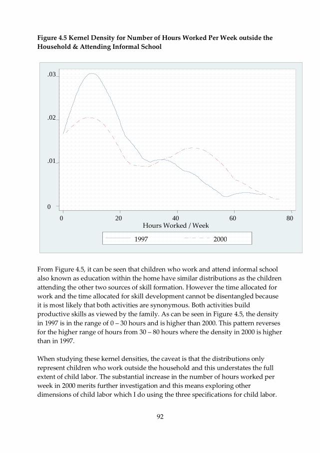
92

Figure 4.5 Kernel Density for Number of Hours Worked Per Week outside the

Household & Attending Informal School

From Figure 4.5, it can be seen that children who work and attend informal school

also known as education within the home have similar distributions as the children

attending the other two sources of skill formation. However the time allocated for

work and the time allocated for skill development cannot be disentangled because

it is most likely that both activities are synonymous. Both activities build

productive skills as viewed by the family. As can be seen in Figure 4.5, the density

in 1997 is in the range of 0 – 30 hours and is higher than 2000. This pattern reverses

for the higher range of hours from 30 – 80 hours where the density in 2000 is higher

than in 1997.

When studying these kernel densities, the caveat is that the distributions only

represent children who work outside the household and this understates the full

extent of child labor. The substantial increase in the number of hours worked per

week in 2000 merits further investigation and this means exploring other

dimensions of child labor which I do using the three specifications for child labor.

0

.01

.02

.03

0 20 40 60 80 Hours Worked / Week

1997 2000

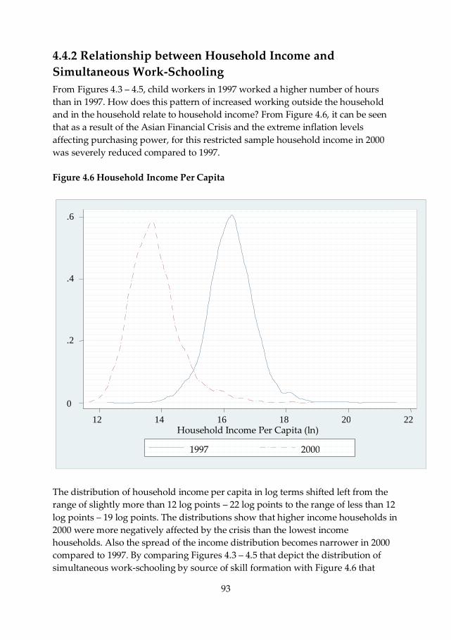
93

4.4.2 Relationship between Household Income and

Simultaneous Work-Schooling

From Figures 4.3 – 4.5, child workers in 1997 worked a higher number of hours

than in 1997. How does this pattern of increased working outside the household

and in the household relate to household income? From Figure 4.6, it can be seen

that as a result of the Asian Financial Crisis and the extreme inflation levels

affecting purchasing power, for this restricted sample household income in 2000

was severely reduced compared to 1997.

Figure 4.6 Household Income Per Capita

The distribution of household income per capita in log terms shifted left from the

range of slightly more than 12 log points – 22 log points to the range of less than 12

log points – 19 log points. The distributions show that higher income households in

2000 were more negatively affected by the crisis than the lowest income

households. Also the spread of the income distribution becomes narrower in 2000

compared to 1997. By comparing Figures 4.3 – 4.5 that depict the distribution of

simultaneous work-schooling by source of skill formation with Figure 4.6 that

0

.2

.4

.6

12 14 16 18 20 22 Household Income Per Capita (ln)

1997 2000

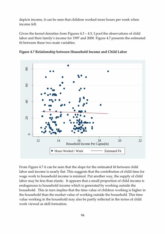
94

depicts income, it can be seen that children worked more hours per week when

income fell.

Given the kernel densities from Figures 4.3 – 4.5, I pool the observations of child

labor and their family’s income for 1997 and 2000. Figure 4.7 presents the estimated

fit between these two main variables.

Figure 4.7 Relationship between Household Income and Child Labor

020

40

60

80

Hours

Work

ed /

Week

12 14 16 18 20 22Household Income Per Capita(ln)

Hours Worked / Week Estimated Fit

From Figure 4.7 it can be seen that the slope for the estimated fit between child

labor and income is nearly flat. This suggests that the contribution of child time for

wage work to household income is minimal. Put another way, the supply of child

labor may be less than elastic. It appears that a small proportion of child income is

endogenous to household income which is generated by working outside the

household. This in turn implies that the time value of children working is higher in

the household than the market value of working outside the household. This time

value working in the household may also be partly reflected in the terms of child

work viewed as skill formation.

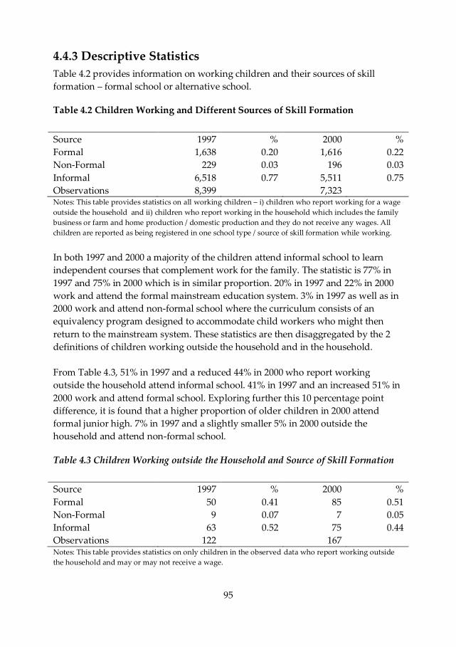
95

4.4.3 Descriptive Statistics

Table 4.2 provides information on working children and their sources of skill

formation – formal school or alternative school.

Table 4.2 Children Working and Different Sources of Skill Formation

Source 1997 % 2000 %

Formal 1,638 0.20 1,616 0.22

Non-Formal 229 0.03 196 0.03

Informal 6,518 0.77 5,511 0.75

Observations 8,399 7,323 Notes: This table provides statistics on all working children – i) children who report working for a wage

outside the household and ii) children who report working in the household which includes the family

business or farm and home production / domestic production and they do not receive any wages. All

children are reported as being registered in one school type / source of skill formation while working.

In both 1997 and 2000 a majority of the children attend informal school to learn

independent courses that complement work for the family. The statistic is 77% in

1997 and 75% in 2000 which is in similar proportion. 20% in 1997 and 22% in 2000

work and attend the formal mainstream education system. 3% in 1997 as well as in

2000 work and attend non-formal school where the curriculum consists of an

equivalency program designed to accommodate child workers who might then

return to the mainstream system. These statistics are then disaggregated by the 2

definitions of children working outside the household and in the household.

From Table 4.3, 51% in 1997 and a reduced 44% in 2000 who report working

outside the household attend informal school. 41% in 1997 and an increased 51% in

2000 work and attend formal school. Exploring further this 10 percentage point

difference, it is found that a higher proportion of older children in 2000 attend

formal junior high. 7% in 1997 and a slightly smaller 5% in 2000 outside the

household and attend non-formal school.

Table 4.3 Children Working outside the Household and Source of Skill Formation

Source 1997 % 2000 %

Formal 50 0.41 85 0.51

Non-Formal 9 0.07 7 0.05

Informal 63 0.52 75 0.44

Observations 122 167 Notes: This table provides statistics on only children in the observed data who report working outside

the household and may or may not receive a wage.

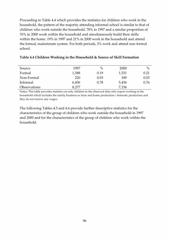
96

Proceeding to Table 4.4 which provides the statistics for children who work in the

household, the pattern of the majority attending informal school is similar to that of

children who work outside the household. 78% in 1997 and a similar proportion of

76% in 2000 work within the household and simultaneously build their skills

within the home. 19% in 1997 and 21% in 2000 work in the household and attend

the formal, mainstream system. For both periods, 3% work and attend non-formal

school.

Table 4.4 Children Working in the Household & Source of Skill Formation

Source 1997 % 2000 %

Formal 1,588 0.19 1,531 0.21

Non-Formal 220 0.03 189 0.03

Informal 6,456 0.78 5,436 0.76

Observations 8,277 7,156 Notes: This table provides statistics on only children in the observed data who report working in the

household which includes the family business or farm and home production / domestic production and

they do not receive any wages.

The following Tables 4.5 and 4.6 provide further descriptive statistics for the

characteristics of the group of children who work outside the household in 1997

and 2000 and for the characteristics of the group of children who work within the

household.

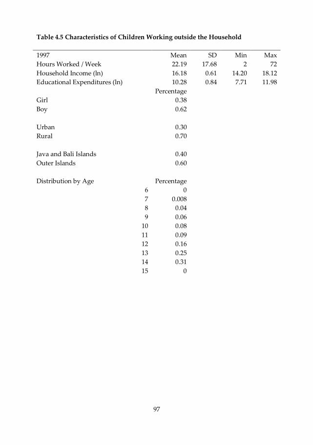
97

Table 4.5 Characteristics of Children Working outside the Household

1997 Mean SD Min Max

Hours Worked / Week 22.19 17.68 2 72

Household Income (ln) 16.18 0.61 14.20 18.12

Educational Expenditures (ln) 10.28 0.84 7.71 11.98

Percentage

Girl 0.38

Boy 0.62

Urban 0.30

Rural 0.70

Java and Bali Islands 0.40

Outer Islands 0.60

Distribution by Age Percentage

6 0

7 0.008

8 0.04

9 0.06

10 0.08

11 0.09

12 0.16

13 0.25

14 0.31

15 0

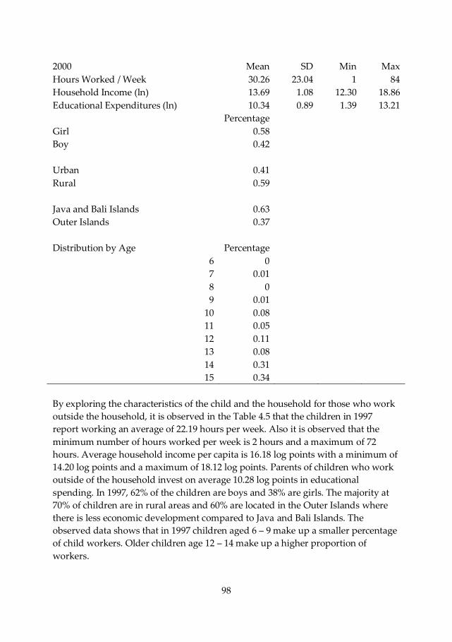
98

2000 Mean SD Min Max

Hours Worked / Week 30.26 23.04 1 84

Household Income (ln) 13.69 1.08 12.30 18.86

Educational Expenditures (ln) 10.34 0.89 1.39 13.21

Percentage

Girl 0.58

Boy 0.42

Urban 0.41

Rural 0.59

Java and Bali Islands 0.63

Outer Islands 0.37

Distribution by Age Percentage

6 0

7 0.01

8 0

9 0.01

10 0.08

11 0.05

12 0.11

13 0.08

14 0.31

15 0.34

By exploring the characteristics of the child and the household for those who work

outside the household, it is observed in the Table 4.5 that the children in 1997

report working an average of 22.19 hours per week. Also it is observed that the

minimum number of hours worked per week is 2 hours and a maximum of 72

hours. Average household income per capita is 16.18 log points with a minimum of

14.20 log points and a maximum of 18.12 log points. Parents of children who work

outside of the household invest on average 10.28 log points in educational

spending. In 1997, 62% of the children are boys and 38% are girls. The majority at

70% of children are in rural areas and 60% are located in the Outer Islands where

there is less economic development compared to Java and Bali Islands. The

observed data shows that in 1997 children aged 6 – 9 make up a smaller percentage

of child workers. Older children age 12 – 14 make up a higher proportion of

workers.

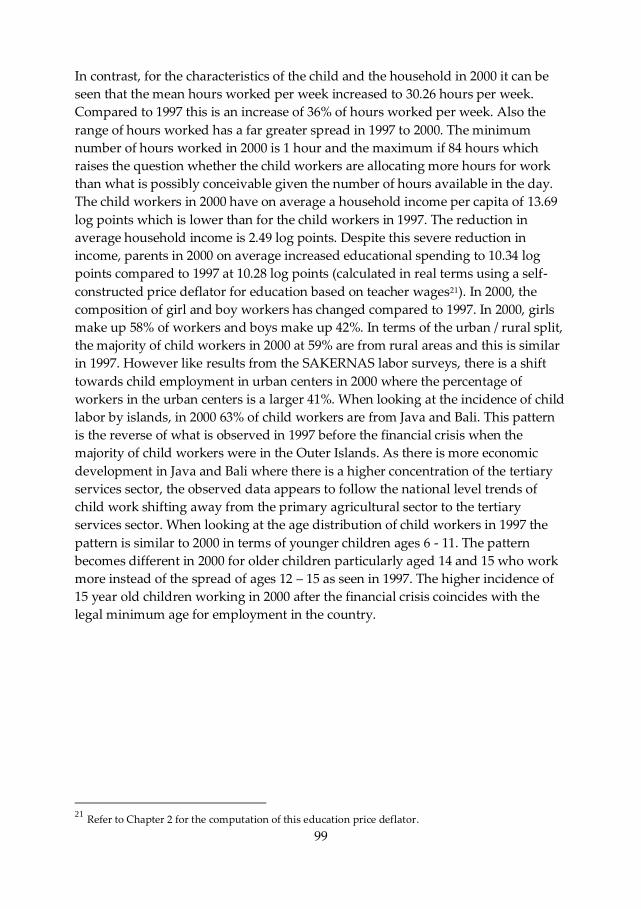
99

In contrast, for the characteristics of the child and the household in 2000 it can be

seen that the mean hours worked per week increased to 30.26 hours per week.

Compared to 1997 this is an increase of 36% of hours worked per week. Also the

range of hours worked has a far greater spread in 1997 to 2000. The minimum

number of hours worked in 2000 is 1 hour and the maximum if 84 hours which

raises the question whether the child workers are allocating more hours for work

than what is possibly conceivable given the number of hours available in the day.

The child workers in 2000 have on average a household income per capita of 13.69

log points which is lower than for the child workers in 1997. The reduction in

average household income is 2.49 log points. Despite this severe reduction in

income, parents in 2000 on average increased educational spending to 10.34 log

points compared to 1997 at 10.28 log points (calculated in real terms using a self-

constructed price deflator for education based on teacher wages21). In 2000, the

composition of girl and boy workers has changed compared to 1997. In 2000, girls

make up 58% of workers and boys make up 42%. In terms of the urban / rural split,

the majority of child workers in 2000 at 59% are from rural areas and this is similar

in 1997. However like results from the SAKERNAS labor surveys, there is a shift

towards child employment in urban centers in 2000 where the percentage of

workers in the urban centers is a larger 41%. When looking at the incidence of child

labor by islands, in 2000 63% of child workers are from Java and Bali. This pattern

is the reverse of what is observed in 1997 before the financial crisis when the

majority of child workers were in the Outer Islands. As there is more economic

development in Java and Bali where there is a higher concentration of the tertiary

services sector, the observed data appears to follow the national level trends of

child work shifting away from the primary agricultural sector to the tertiary

services sector. When looking at the age distribution of child workers in 1997 the

pattern is similar to 2000 in terms of younger children ages 6 - 11. The pattern

becomes different in 2000 for older children particularly aged 14 and 15 who work

more instead of the spread of ages 12 – 15 as seen in 1997. The higher incidence of

15 year old children working in 2000 after the financial crisis coincides with the

legal minimum age for employment in the country.

21 Refer to Chapter 2 for the computation of this education price deflator.

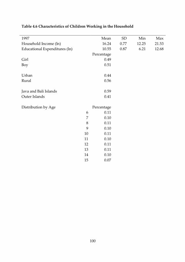
100

Table 4.6 Characteristics of Children Working in the Household

1997 Mean SD Min Max

Household Income (ln) 16.24 0.77 12.25 21.53

Educational Expenditures (ln) 10.55 0.87 6.21 12.68

Percentage

Girl 0.49

Boy 0.51

Urban 0.44

Rural 0.56

Java and Bali Islands 0.59

Outer Islands 0.41

Distribution by Age Percentage

6 0.11

7 0.10

8 0.11

9 0.10

10 0.11

11 0.10

12 0.11

13 0.11

14 0.10

15 0.07

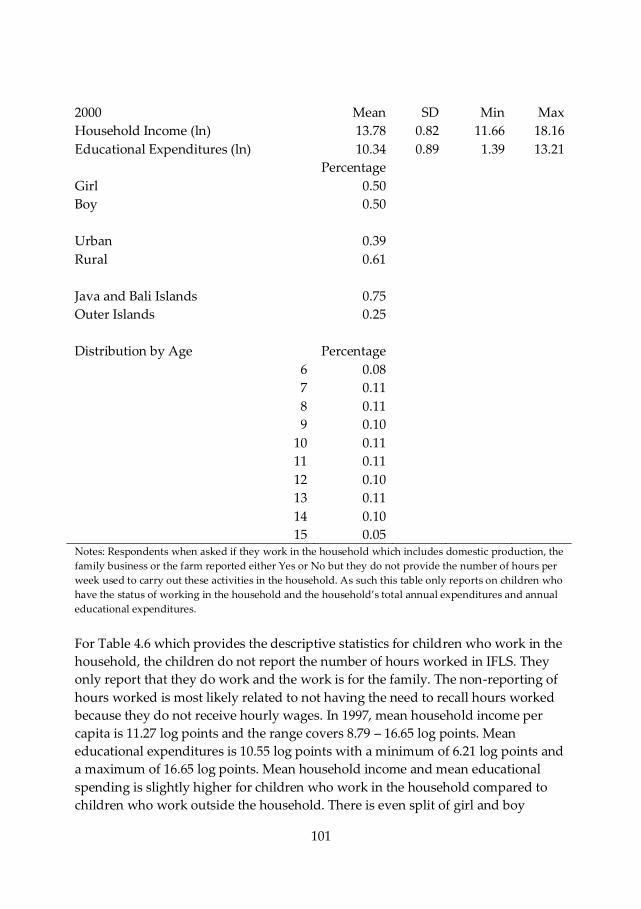
101

2000 Mean SD Min Max

Household Income (ln) 13.78 0.82 11.66 18.16

Educational Expenditures (ln) 10.34 0.89 1.39 13.21

Percentage

Girl 0.50

Boy 0.50

Urban 0.39

Rural 0.61

Java and Bali Islands 0.75

Outer Islands 0.25

Distribution by Age Percentage

6 0.08

7 0.11

8 0.11

9 0.10

10 0.11

11 0.11

12 0.10

13 0.11

14 0.10

15 0.05 Notes: Respondents when asked if they work in the household which includes domestic production, the

family business or the farm reported either Yes or No but they do not provide the number of hours per

week used to carry out these activities in the household. As such this table only reports on children who

have the status of working in the household and the household’s total annual expenditures and annual

educational expenditures.

For Table 4.6 which provides the descriptive statistics for children who work in the

household, the children do not report the number of hours worked in IFLS. They

only report that they do work and the work is for the family. The non-reporting of

hours worked is most likely related to not having the need to recall hours worked

because they do not receive hourly wages. In 1997, mean household income per

capita is 11.27 log points and the range covers 8.79 – 16.65 log points. Mean

educational expenditures is 10.55 log points with a minimum of 6.21 log points and

a maximum of 16.65 log points. Mean household income and mean educational

spending is slightly higher for children who work in the household compared to

children who work outside the household. There is even split of girl and boy

102

workers in 1997. Like children who work outside the household in 1997, the

majority who work in the household at 56% are from rural areas. But 59% are

located in Java and Bali and 41% are located in the Outer Islands. This is the reverse

of children who work outside the household. In terms of the age distribution, the

children ages 6 – 14 are evenly spread out in 1997 where there does not appear to

be any difference whether a younger or older child works in the household. The

slight exception is that a smaller percentage of 15 year olds work in the household.

As a comparison, in 2000 for children who work in the household, average

household income per capita is higher than in 1997. After the crisis, average

household income is 11.87 log points with a minimum of 9.86 log points and a

maximum of 14.78 log points. However mean educational investments at 10.34 log

points are lower in 2000 for children who work in the household compared to 1997.

Also the range for educational investments has severely deteriorated after the crisis

in terms of the minimum value is at a low of 1.39 log points. However the range

has a greater spread compared to 1997 with the maximum value at a high of 13.21

log points. In terms of gender and the urban / rural split, there is the same pattern

in both 1997 and 2000. The incidence of child labor in 2000 shows the same pattern

as in 1997 in terms of the majority who work in the household being located in Java

and Bali Islands. The age distribution for the children who work for the family in

the 2000 remains the same as in 1997 including 15 year old children working less at

home compared to the children aged 6 – 14.

4.5 Results In Table 4.7, I present the results for the first sample that consists of children who

work and attend school and children who do not work and only attend school full

time. Full time schooling is in terms of any of the three sources of skill formation.

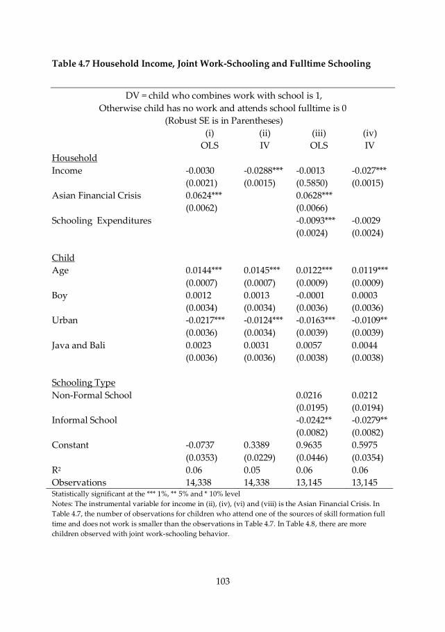
103

Table 4.7 Household Income, Joint Work-Schooling and Fulltime Schooling

DV = child who combines work with school is 1,

Otherwise child has no work and attends school fulltime is 0

(Robust SE is in Parentheses)

(i) (ii) (iii) (iv)

OLS IV OLS IV

Household

Income -0.0030

(0.0021)

-0.0288***

(0.0015)

-0.0013

(0.5850)

-0.027***

(0.0015)

Asian Financial Crisis 0.0624***

(0.0062)

0.0628***

(0.0066)

Schooling Expenditures -0.0093***

(0.0024)

-0.0029

(0.0024)

Child

Age 0.0144***

(0.0007)

0.0145***

(0.0007)

0.0122***

(0.0009)

0.0119***

(0.0009)

Boy 0.0012

(0.0034)

0.0013

(0.0034)

-0.0001

(0.0036)

0.0003

(0.0036)

Urban -0.0217***

(0.0036)

-0.0124***

(0.0034)

-0.0163***

(0.0039)

-0.0109**

(0.0039)

Java and Bali 0.0023

(0.0036)

0.0031

(0.0036)

0.0057

(0.0038)

0.0044

(0.0038)

Schooling Type

Non-Formal School 0.0216

(0.0195)

0.0212

(0.0194)

Informal School -0.0242**

(0.0082)

-0.0279**

(0.0082)

Constant -0.0737

(0.0353)

0.3389

(0.0229)

0.9635

(0.0446)

0.5975

(0.0354)

R2 0.06 0.05 0.06 0.06

Observations 14,338 14,338 13,145 13,145 Statistically significant at the *** 1%, ** 5% and * 10% level

Notes: The instrumental variable for income in (ii), (iv), (vi) and (viii) is the Asian Financial Crisis. In

Table 4.7, the number of observations for children who attend one of the sources of skill formation full

time and does not work is smaller than the observations in Table 4.7. In Table 4.8, there are more

children observed with joint work-schooling behavior.

104

In columns (i) and (ii) the regressions do not include the endogenous explanatory

variables, schooling expenditures and schooling type. I find that the OLS estimate

in (i) for household income per capita is negative and comparable in magnitude to

the IV estimate in (ii). However the IV estimate is statistically significant at the 1%

level and the OLS estimate is not significant. As expected when income is lower,

the child combines work with schooling and does not attend school full time.

Correspondingly, an increase in schooling related expenditures increases the

likelihood that the child will attend school full time. However the effect of

schooling expenditures on the child’s work – schooling behavior is smaller than the

effect of income. In columns (iii) and (iv) the coefficient size for schooling

expenditures is smaller than for income. While the OLS estimate for these

expenditures is statistically significant it is no longer the case for the IV estimate. In

terms of the age effect, I find that across columns (i) to (iv), the older the child is,

the higher the propensity for the child to work. This is similar to the national level

trend highlighted in Figure 4.1. The OLS and IV estimates for age are similar in

magnitude across the four columns and all are statistically significant at the 1%

level. As the OLS and IV estimates are similar, there is little bias. I also find that

children who reside in urban centers have the propensity to attend school full time

and not work. This is a statistically significant result across (i) to (iv) which is when

the endogenous explanatory variables are not included and when included. I do

not find any other significant results to explore further in terms of child attributes.

This includes the gender of the child which suggests there is minimal bias whether

a boy or a girl attends school full time or works full time. When I focus on the three

sources of skill formation, I find that the provision of non-formal schooling by non-

governmental organizations including religious schools increases the propensity of

joint work-schooling. This is consistent with the design of non-formal schools for

accommodating the skill development needs of child workers. However this result

is not statistically significant. In contrast, when the source of skill development

comes from the family, there is a positive relationship between attending school

full time and not working. The OLS and IV estimates have similar coefficients and

are statistically significant at the 5% level.

In Table 4.8, I present the results that use the dependent variable of children who

work outside the household combined with attending school and children who

work within the household while attending school.

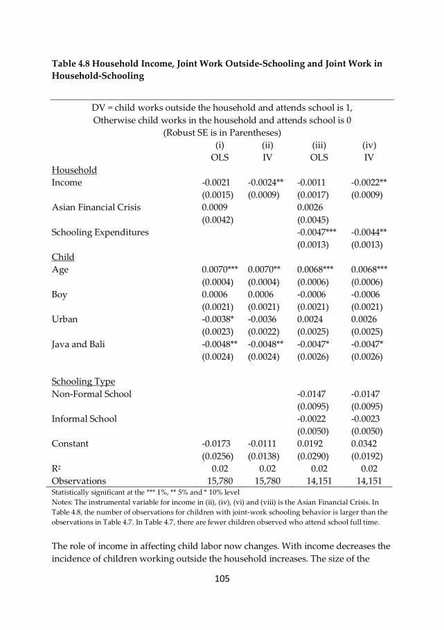
105

Table 4.8 Household Income, Joint Work Outside-Schooling and Joint Work in

Household-Schooling

DV = child works outside the household and attends school is 1,

Otherwise child works in the household and attends school is 0

(Robust SE is in Parentheses)

(i) (ii) (iii) (iv)

OLS IV OLS IV

Household

Income -0.0021

(0.0015)

-0.0024**

(0.0009)

-0.0011

(0.0017)

-0.0022**

(0.0009)

Asian Financial Crisis 0.0009

(0.0042)

0.0026

(0.0045)

Schooling Expenditures -0.0047***

(0.0013)

-0.0044**

(0.0013)

Child

Age 0.0070***

(0.0004)

0.0070**

(0.0004)

0.0068***

(0.0006)

0.0068***

(0.0006)

Boy 0.0006

(0.0021)

0.0006

(0.0021)

-0.0006

(0.0021)

-0.0006

(0.0021)

Urban -0.0038*

(0.0023)

-0.0036

(0.0022)

0.0024

(0.0025)

0.0026

(0.0025)

Java and Bali -0.0048**

(0.0024)

-0.0048**

(0.0024)

-0.0047*

(0.0026)

-0.0047*

(0.0026)

Schooling Type

Non-Formal School -0.0147

(0.0095)

-0.0147

(0.0095)

Informal School -0.0022

(0.0050)

-0.0023

(0.0050)

Constant -0.0173

(0.0256)

-0.0111

(0.0138)

0.0192

(0.0290)

0.0342

(0.0192)

R2 0.02 0.02 0.02 0.02

Observations 15,780 15,780 14,151 14,151 Statistically significant at the *** 1%, ** 5% and * 10% level

Notes: The instrumental variable for income in (ii), (iv), (vi) and (viii) is the Asian Financial Crisis. In

Table 4.8, the number of observations for children with joint-work schooling behavior is larger than the

observations in Table 4.7. In Table 4.7, there are fewer children observed who attend school full time.

The role of income in affecting child labor now changes. With income decreases the

incidence of children working outside the household increases. The size of the

106

income coefficient as reported by OLS and IV is similar to the size of the income

coefficient when the dependent variable is specified as whether a child attends

school full time (Table 4.7). However only the IV estimate is statistically significant

and this is at the 5% level. Household investment in schooling as represented by

schooling expenditures in columns (iii) and (iv) have the same relationship as

income in terms of how it relates to child labor. With a fall in schooling

expenditures, the incidence of children working outside the household increases.

The OLS and IV estimates for spending are similar in magnitude and statistically

significant. More importantly, the size of the coefficients for schooling expenditures

is now larger than for household income. The significance of schooling

expenditures when child labor is now specified in terms of working outside or

within the household suggest that when parents choose to keep their children

working in the home, there are likely to be elements of skill formation. As

described in Chapter 2, children complement learning in the informal school with

individual courses provided by the Ministry of Education. Parents can make these

investments in their children when they are in the home enterprise but this may be

less likely when the child works outside of the household for an employer.

In comparing the relationship between an income reduction and the incidence of

joint work-schooling (Table 4.7) with the relationship between an income reduction

and the incidence of working outside of the household (Table 4.8), decreases in

income drive the shift towards joint work-schooling. But the reduction in income

does not determine if the child will have a higher likelihood of working outside the

household or in the household. This can be interpreted as a fall in income causes

simultaneous work-schooling decisions but working can just as likely take place

outside the household or in the household.

The relationship between the age of the child and the incidence of working is also

borne out in Table 4.8 but now specifically in terms of an older child is more likely

to work outside the household while attending school. This result is statistically

significant at the 1% level. This finding is consistent with the intuition that when

older the child is expected to be better equipped to manage the safety and health

risks of working outside without parental supervision. In Table 4.8, I now have a

new result that I did not have from Table 4.8 which is related to the child’s

residential location. On the one hand residence in Java and Bali Islands does not

play a substantial role in determining whether a child is in school or at work full

time. But on the other hand, location becomes important for whether a child works

outside the household or in the household. From Table 4.8, across columns (i) – (iv)

it can be seen a child worker residing in Java and Bali Islands will work outside the

household and attend school and this is statistically significant. This strongly

suggests that there are more economic opportunities available in Java and Bali

compared to the Outer Islands that have lower levels of economic development. As

107

such when the child has to work, it is more likely that the child will work outside of

the household because the relative returns will likely be higher than what is gained

by working for the family in the household. I also find that the source of skill

formation that now plays a noticeable role is non-governmental organization run

schools for child laborers. This coefficient has a negative relationship with children

working outside the household which can be interpreted as non-formal schooling

reduces the incidence of working outside the household while attending school.

This is consistent with the design and availability of this school type to

accommodate the needs of child laborers. Schooling time is structured around the

working hours of the child laborers so as not to deprive them of the opportunities

for skill development. However the negative relationship between non-formal

schooling and working outside the household is not statistically significant. The

relationship between informal schooling and working outside the household is also

negative and not statistically significant. However the size of the coefficient for

informal school is smaller than for non-formal school. This implies that non-formal

schools have a more important influence than informal schools in the skill

development of children working outside of the household.

Table 4.9 shows the results for the specification of child labor in terms of the

number of hours worked per week outside the household while attending school.

Given the kernel densities from Figures 4.3 – 4.5, it was found that children in 1997

worked more hours per week while attending school compared to children in 2000.

This raises the question of how much time is available for a child to work and to

learn while contributing to household income.

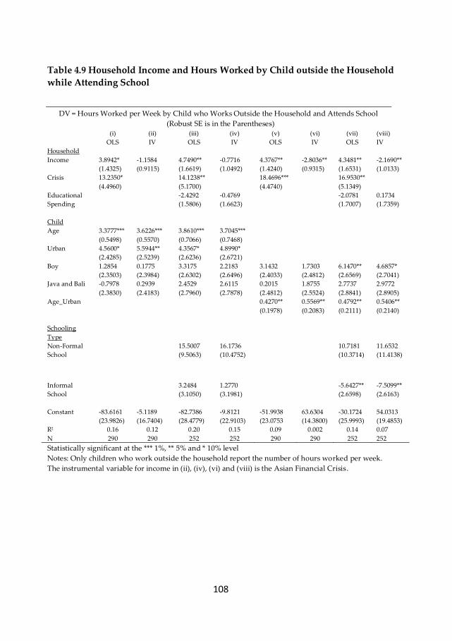
108

Table 4.9 Household Income and Hours Worked by Child outside the Household

while Attending School

DV = Hours Worked per Week by Child who Works Outside the Household and Attends School

(Robust SE is in the Parentheses)

(i) (ii) (iii) (iv) (v) (vi) (vii) (viii)

OLS IV OLS IV OLS IV OLS IV

Household

Income 3.8942*

(1.4325)

-1.1584

(0.9115)

4.7490**

(1.6619)

-0.7716

(1.0492)

4.3767**

(1.4240)

-2.8036**

(0.9315)

4.3481**

(1.6531)

-2.1690**

(1.0133)

Crisis 13.2350*

(4.4960)

14.1238**

(5.1700)

18.4696***

(4.4740)

16.9530**

(5.1349)

Educational

Spending

-2.4292

(1.5806)

-0.4769

(1.6623)

-2.0781

(1.7007)

0.1734

(1.7359)

Child

Age 3.3777***

(0.5498)

3.6226***

(0.5570)

3.8610***

(0.7066)

3.7045***

(0.7468)

Urban 4.5600*

(2.4285)

5.5944**

(2.5239)

4.3567*

(2.6236)

4.8990*

(2.6721)

Boy 1.2854

(2.3503)

0.1775

(2.3984)

3.3175

(2.6302)

2.2183

(2.6496)

3.1432

(2.4033)

1.7303

(2.4812)

6.1470**

(2.6569)

4.6857*

(2.7041)

Java and Bali -0.7978

(2.3830)

0.2939

(2.4183)

2.4529

(2.7960)

2.6115

(2.7878)

0.2015

(2.4812)

1.8755

(2.5524)

2.7737

(2.8841)

2.9772

(2.8905)

Age_Urban 0.4270**

(0.1978)

0.5569**

(0.2083)

0.4792**

(0.2111)

0.5406**

(0.2140)

Schooling

Type

Non-Formal

School

15.5007

(9.5063)

16.1736

(10.4752)

10.7181

(10.3714)

11.6532

(11.4138)

Informal

School

3.2484

(3.1050)

1.2770

(3.1981)

-5.6427**

(2.6598)

-7.5099**

(2.6163)

Constant -83.6161

(23.9826)

-5.1189

(16.7404)

-82.7386

(28.4779)

-9.8121

(22.9103)

-51.9938

(23.0753

63.6304

(14.3800)

-30.1724

(25.9993)

54.0313

(19.4853)

R2 0.16 0.12 0.20 0.15 0.09 0.002 0.14 0.07

N 290 290 252 252 290 290 252 252

Statistically significant at the *** 1%, ** 5% and * 10% level

Notes: Only children who work outside the household report the number of hours worked per week.

The instrumental variable for income in (ii), (iv), (vi) and (viii) is the Asian Financial Crisis.

109

From column (i) in Table 4.9, the OLS estimate for income is positive and

statistically significant at the 10% level. When household income decreases by one

log point, a child works nearly four hours less per week. The IV estimate in column

(ii) negates this relationship where when household income decreases by one log

point, the child works one more hour per week. But this result is statistically

insignificant. In comparing the OLS and IV estimates, there is selection bias in the

observed data where lower income households have children who work fewer

hours outside the household. The different directions of the OLS and IV estimates

for household income also hold in columns (iii) and (iv) when the endogenous

explanatory variables are included. In terms of schooling expenditures, its effect on

the number of hours worked outside the household is miniscule. This appears to be

consistent with the findings in Table 4.9 when child labor is specified in terms of

working outside or within the household. This implies that parents are less inclined

to invest in the skill formation process when the child works outside for an

employer.

As per the previous two specifications for the dependent variable, the OLS and IV

estimates for age reinforce the finding that as the child is older, the incidence and

intensity of child labor increases. The results across columns (i) – (iv) show that

when the child is older by a year, the child works over three hours more per week.

This is statistically significant at the 1% level. This strongly suggests that it is more

the age of the child worker that shifts a child’s time more towards work outside the

household than variations in household income. In terms of geographical factors, I

find that children in urban centers across all the main islands work on average four

hours more per week and this is statistically significant at the 1% level. This result

can be seen across columns (i) – (iv). The IV estimates are a half hour to an hour

higher than the OLS estimates for each week of work and this is most likely due to

attenuation bias.

Because of the statistically significant results from the age and urban center

exogenous covariates, I now interact the two covariates and run the regressions

from columns (v) – (viii) in Table 4.9. I now have different results for the main

relationship of interest which is income and hours worked per week. The OLS

estimates for income are positive and larger than for the IV estimates which mean

that the OLS estimates are overstating the relationship between income and hours,

due to omitted variables. Using the IV estimates from (vi) and (viii) and comparing

them with the IV estimates from (ii) and (iv), it can be seen that when income

decreases by one log point, the child works two hours more per week controlling

for the child’s age and urban location. This estimate is statistically significant at the

5% level. This finding also reflects the selection bias that lower income households

have children who work fewer hours outside the household. When I study the

interaction between age and urban center, I see that the IV estimates in (vi) and

110

(viii) are slightly higher than the OLS estimates in (v) and (vii) which are likely

related to attenuation bias. It can be seen that when the child is older by a year and

residing in an urban center, the child works 30 minutes more per week and this

finding is statistically significant at the 5% level. This interaction produces

coefficient sizes that are noticeably smaller compared to the prior separate

estimates on age and urban center in (i) – (iv). Another new finding from this

additional specification can be seen in columns (vii) and (viii) where boys tend to

spend more time outside the household working compared to girls. The OLS

estimate is 6 additional hours of work per week, statistically significant at the 5%

level and the IV estimate is at a lower 4.5 hours of more work per week statistically

significant at the 10% level. This strongly implies that there is a gender bias where

boys tend to work outside the household compared to girls and while working

outside for a wage or an in-kind transfer, boys increase hours worked more than

girls. However if the child worker is combining work outside with gaining skills

from informal schooling, hours worked per week fall substantially. When

schooling type as endogenous explanatory variables are included into the

additional specification of the interaction of age and urban center, accounting for

attenuation bias, the child works 7 hours less per week. This finding can be seen in

the IV estimate in column (viii) which is statistically significant at the 5% level. An

interpretation for this finding is that the practice of the family enterprise with child

apprenticeships downplays the need for the child’s market income to complement

household income when there is reduced income. The returns to work for the

family appear to be higher than the returns to work in the market. In addition, by

being an apprentice, the child’s skill formation process continues and this is less

likely when the child works outside the household.

4.6 Conclusions

This chapter has provided evidence on the variations in simultaneous work-

schooling behavior when income falls. I used different operational definitions for

the joint work-schooling decision: joint work and schooling, joint work within the

household and schooling, joint work outside the household and schooling; and

number of hours worked per week and schooling. A fall in income results in a shift

away from full time schooling to joint work-schooling. An income decrease is also

found to increase the propensity to shift away from schooling and towards more

work for children who demonstrate joint work-schooling behavior. But it is not

clear whether the increased incidence of working takes place outside or within the

household. When isolating only child work behavior outside the household for

wages or in-kind transfers, it is found that an income reduction increases the

number of hours worked per week but the increase is small. A one log point

decrease in income only increases work by 2 hours in a week which is not likely to

conflict with time for schooling. To reconcile these findings, a fall in income does

111

increase the propensity of simultaneous work-schooling behavior. However this

does not appear to be captured by the child’s contribution to household income.

Instead the reduction in income may be compensated by a higher relative value of

child time used for work. As such, income does not appear to be the main influence

for the incidence and intensity of child labor.

The main influence driving joint work-schooling is the age of the child. It is more

likely that the child who already demonstrates simultaneous work-schooling

behavior from an age as young as 6 is driven to work more when s/he is older.

When the child is 12 years old, there is a higher propensity for the child to work

outside the household while attending school. In addition this appears to be an

urban phenomenon in Indonesia where wage opportunities are higher in areas

with more economic development. As the 12 year old child becomes older until

s/he reaches the legal employment age of 15, the hours worked per week increase

and there is a greater shift towards full time work. This strongly implies that if the

child is in the formal school system in an urban center, the age range of 12 – 15 is

where the risk increases that the child will fail to complete junior high. This implies

that human capital accumulation will peak at the completion of primary school at

age 12.

This chapter has also provided insight into the schooling choices of child workers –

formal school, non-formal school or informal school. On the one hand the extent of

child labor is arguably overstated if the child is an apprentice in the family

enterprise where work and learning activity are occurring simultaneously; both

types of activity are the one and the same where work is carried out within the

household. As there are productive skills built during the apprenticeship which

provide social returns to the household if not private returns in the market, human

capital accumulation does not appear to be impaired. The child’s health and safety

are also more likely to be assured compared to if the child works outside the

household unsupervised by the parents. On the other hand the extent of child labor

is likely to be understated because in this chapter, a main limitation is that there is

no data available on the type of activity that is carried out. Activities in the

household that can be physically harmful or do not require any skills such as

mundane, repetitive tasks are not observed in the data. As such the child who shifts

more towards work and away from learning may be less likely to build human

capital.

From the perspective of the national education system, the institutional recognition

of both the informal school and non-formal school suggests that the relative value

of time working outside or within the household is higher than schooling for some

families. This then implies that in certain areas particularly urban centers, parents

perceive that the returns to schooling are low. The presence and development of

112

the informal school and non-formal school may then be an appropriate educational

policy response to ensure that economically active children aged 6 – 15 are

guaranteed some form of schooling. However another limitation of this chapter is

that there is no wage data available to assess this to what extent the returns to

schooling are lower than the returns to work outside or within the household.

113

5. Dynamic Complementarity of Investment in

Education

114

5.1 Introduction

Education is generally considered as an important investment for economic

growth. Optimal investments in human capital depend on the direct and

opportunity costs of schooling and the future expected benefits and are thus not

determined by parental income. If education is only considered to be a

consumption good income would matter. But in Indonesia, monetary constraints

together with other high priority expenditures could explain that parents invest

less than is optimal in their children’s education. This is because parents may have

a preference for spending on other urgent issues and perhaps have a preference for

their children to work or to help within the household. Alternative explanations for

sub-optimal investment would be that poorer parents differ in their characteristics

from richer parents and that these characteristics rather than income explain

differences in educational investment. These characteristics could include how they

vthe future expected benefits from the human capital accumulated by their

children. These benefits could be both private and social.

The aims of this chapter are the following. The first aim is to investigate how

income has a causal relationship with educational expenditures in Indonesia. The

second aim is to determine whether time spent on schooling by Indonesian

children is related to income. The third aim is investigate whether Indonesian

parents respond to the expected future benefits of education in their current

educational expenditures. To identify causality, we use the Asian Financial Crisis in

Indonesia as a natural experiment to investigate educational expenditures. In this

way, we obtain estimates of the impact of income on educational expenditures and

time used for schooling while holding constant parental characteristics. The

difference in the parameters between parents of children who have just started

junior high and parents of children who have already attained a few years of a

junior high education reveals whether parents react to differences in returns. Due

to dynamic complementarity in the accumulation of human capital, the loss in

returns due to lower investments for children in later grades of junior high is

higher. Using repeated cross sections from 1997 and 2000, we find that about 80%

of the cross-sectional link between income and educational expenditures is caused

by differences in income. The remaining 20% is related to unobserved parental

characteristics or to unobserved child characteristics. Lower educational

expenditures due to less income are highly compensated by time investments. The

effect of time investments is 50% stronger than suggested by cross-sectional

evidence. This strongly implies that income related parental characteristics explain

a substantial part of these compensating time investments. Finally the reduction in

educational expenditures is much lower for children who have already attained a

115

few years of junior high education. This implies that parents do take into account

the loss in returns related to previous investments on the stock of human capital

accumulated. Or put in another way, there is loss aversion. Thus this suggests that

the future expected benefits of their children’s education do play a role in

investment decisions. Taken together these results reveal that monetary constraints

do restrict parents in their educational expenditures, that they are concerned with

future returns; and that especially parents with favorable characteristics

compensate reductions in educational expenditures by letting their higher ability

children spend more time in school.

This chapter is related to the literature on educational investments in developing

countries. Optimal parental investments based on future expected benefits have

tended to be concentrated on potential lost productivity from premature school

dropout given credit constraints. Available estimates indicate that schooling in

developing countries has a high payoff of a 25 – 30 percent real rate of return,

especially for lower levels of schooling (e.g. Psacharopoulos 1994; Psacharopoulos

and Patrinos 2004). At the same time, school completion rates in developing

countries are very low (Lockheed and Verspoor 1991). To reconcile the

contradiction between high rates of return with low schooling attainment school

quality and quantity of schooling completed may be positively correlated, leading

to upward biases in the rates of return estimated by traditional approaches

(Behrman and Birdsall 1983; Hanushek, Lavy and Hitomi, 2008). In his review of

the literature on education investments comparing developed and developing

countries, Hanushek sums up that parents in developing countries may not invest

more in education if their children’s educational achievement and abilities do not

translate into earnings opportunities outside of school (1995, 2008).

This chapter is also related to the theory of the technology of skill formation in the

child’s life cycle (Cunha et al 2004, 2005; Cunha and Heckman, 2007; Caucutt and

Lochner, 2008). Cameron & Heckman (2001), Keane & Wolpin (2001) and Cameron

& Taber (2004) explore the positive correlation between college enrollment and

family income. Using different methodology types, the authors argue that short-

run borrowing constraints do not drive schooling decisions such as staying on at

school after the compulsory age. Rather, Cameron & Heckman (2001) argue that

binding lifetime credit constraints alter human capital investment through the

entire childhood and drive the stock of human capital at the time schooling

decisions are made. We take these arguments into consideration for the Indonesian

developing country context where there is no enforced compulsory schooling age,

thus credit constraints can drive schooling decisions at any schooling level.

The contributions of this chapter to the literature are threefold. First, optimal

education investment does include accounting for the loss in returns from previous

116

investments on the stock of human capital that has been accumulated. Put in

another way, sunk costs matter. Second, this chapter expands the Cunha and

Heckman (2007) technology of skill formation structural equation modeling to

instrumental variable estimation. Third, this chapter provides the first piece of

evidence on the technology of skill formation in a developing country.

The rest of the chapter is organized in the following way. In Section 5.2, using the

theoretical framework of the technology of skill formation, we will build a model to

formalize our ideas. In Section 5.3 we outline the empirical strategy, introduce

operational definitions related to the technology of skill formation framework; and

describe the data we use. This is followed by descriptive statistics and results in

Section 5.4. Conclusions are made in Section 5.5.

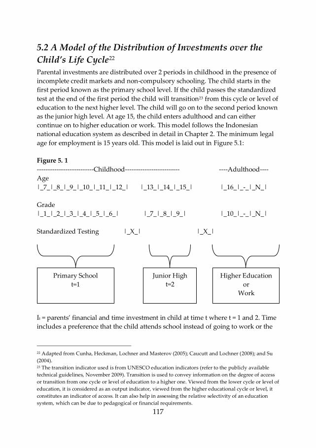
117

5.2 A Model of the Distribution of Investments over the

Child’s Life Cycle22

Parental investments are distributed over 2 periods in childhood in the presence of

incomplete credit markets and non-compulsory schooling. The child starts in the

first period known as the primary school level. If the child passes the standardized

test at the end of the first period the child will transition23 from this cycle or level of

education to the next higher level. The child will go on to the second period known

as the junior high level. At age 15, the child enters adulthood and can either

continue on to higher education or work. This model follows the Indonesian

national education system as described in detail in Chapter 2. The minimum legal

age for employment is 15 years old. This model is laid out in Figure 5.1:

Figure 5. 1

--------------------------Childhood------------------------- ----Adulthood----

Age

|_7_|_8_|_9_|_10_|_11_|_12_| |_13_|_14_|_15_| |_16_|_-_|_N_|

Grade

|_1_|_2_|_3_|_4_|_5_|_6_| |_7_|_8_|_9_| |_10_|_-_|_N_|

Standardized Testing |_X_| |_X_|

It = parents’ financial and time investment in child at time t where t = 1 and 2. Time

includes a preference that the child attends school instead of going to work or the

22 Adapted from Cunha, Heckman, Lochner and Masterov (2005); Caucutt and Lochner (2008); and Su

(2004). 23 The transition indicator used is from UNESCO education indicators (refer to the publicly available

technical guidelines, November 2009). Transition is used to convey information on the degree of access

or transition from one cycle or level of education to a higher one. Viewed from the lower cycle or level of

education, it is considered as an output indicator, viewed from the higher educational cycle or level, it

constitutes an indicator of access. It can also help in assessing the relative selectivity of an education

system, which can be due to pedagogical or financial requirements.

Primary School

t=1

Junior High

t=2

Higher Education

or

Work

118

child can stay at home. It is a function of household income which consists of per

capita consumption Ct and per capita savings Σt

),( tttt CfI

Ct > Σt; Σt≠0 because of incomplete credit markets; Parents’ utility is increasing and

concave.

St for t = 1 and 2 where 1 = skills acquired at the primary school level and 2 = skills

acquired at the junior high level. S1 skills consist of Indonesian language literacy,

math, science, social studies and moral studies. S2 skills consist of Indonesian and

English language literacy, math, science, social studies & moral studies. Implicitly

the stock of skills acquired will depreciate over time as per the Ben-Porath Model

(1967)24. This depreciation rate is dependent on the child’s innate ability.

S0 are initial skills when the child is born. Assume that the child is born to family

with a given occupation and initial skills are correlated with the family

occupation25. The technology of skill formation can be written as

),(1 tttt ISfS

where ft is a stage-t function mapping skill (ability) levels and financial investment

at stage t into skill(ability) levels at t+1. For simplicity we assume that ft is twice

continuously differentiable in its arguments. Its domain of definition is the same

for all inputs that make up the financial investment e.g. books, computers,

contributions to the parent-teacher association, etc. The proportion of inputs may

be different at different stages in childhood, so that the inputs in It may be different

from the inputs at period τ different from t.

Direct complementarity at stage t is defined by the L x K matrix:

tt

t

IS

S

1

2

>0

Higher levels of It raise the productivity of St. Or there is the reverse relationship

where higher levels of St raise the productivity of It

This generalized notation entertains the possibility that some components of skill

can only come together and be productive cumulatively at certain critical periods.

Period t is critical for skill (ability) j if

24 The implicit assumption of this model with reference to the Ben Porath model 25 This assumption follows Endogenous Inequality Theory (Mookherjee and Ray, 2003)

119

0,1

t

jt

I

S

But

,0,1

kt

jkt

I

S k>0

Crucial or sensitive points in time for investment are those where, at the same level

of input St, It, the t

t

I

S

1 are high. More formally, let St = st, It = it, t is a sensitive

period for skill or ability j if

0,,

,1

,

,1

kI

S

I

S

tttttkttkt iIsSt

jt

iIsSkt

jkt

The sensitive time in our model is the period of junior high at t = 2 after the child

has completed and transitioned from primary school at t = 1. This is a sensitive

period in terms of maximizing the returns to education in an incomplete credit

market.

If there is the dynamic complementarity of investment, current investment should

be at a higher level that prior investment. Intuitively, the current level of

expenditures for junior high should be higher because the child is older and all

educational expenditures should cost more. But it is not only age effects driving

expenditures. Our focus is on how much more productivity is gained from having

higher later investments on top of early investments. What the child learns in junior

high are gains in advanced skills in language and math; and the spillovers these

two subjects produce for the other subjects. To illustrate, when in primary school,

the child gains a basic skill in literacy using the Indonesian language. This sets the

stage for the child in junior high to learn a second language, English which

incidentally has similarity in syntax to the Indonesian language. Also the

Indonesian language has adopted much of the modern vocabulary of the English

language. Put simply, early investments in primary school are not productive if

they are not followed up by later investments in junior high.

Proceeding from the theoretical generalized model of the technology of skill

formation, we move on to a reduced form specification and we assume a linear

model. Considering the dynamic complementarity of investment given income we

have the following reduced form:

120

Investmentt = f(Incomet, Skills t-1, Aget) where t covers two periods

Investment at t is for current investment and household income at t is for current

income. Skills have been built up over the entire prior period t-1 to represent a

stock of accumulated human capital. Age represents the current school age of the

child and the schooling level. But there is an endogeneity problem. To be able to

test this model, we use instrumental variable (IV) analysis as detailed in our

empirical strategy in section 4 where the instruments work through the value that

parents have for the future expected benefits of their children’s skills attained,

where the variation in investment at t is owing to parental income at t. A

comparison of the OLS and IV estimators then enable us to determine the extent to

which unobserved parental characteristics influence educational investments. In

section 2, we will describe the institutional context for our investigation.

5.3. Operational Definitions and Empirical Strategy Our empirical strategy consists of a natural experiment with instrumental variable

(IV-2SLS) estimation. We closely follow the parameters in the theoretical model of

the technology of skill formation as can been seen in the applied model in Section

5.2. We proceed to test the causal relationship between income and educational

investments in the presence of credit constraints. We exploit the AFC as the source

of exogenous variation in income in order to carry out IV-2SLS analysis. Because of

the AFC, households incomes are all reduced and it is assumed that there are no

incomes moving in the other direction26. Heterogeneous responses are then

assumed to be with respect to a fall in income. We observe the behavior of rich and

poor households across the income distribution and how they adjust their

investment decisions before and after the AFC. These investment decisions are with

respect to their children transitioning from primary school to junior high. Our

identifying assumption is that the AFC affected educational decisions only through

income and not through other channels.

The data that we use is the RAND Corporation Indonesia Family Life Surveys

(IFLS) Wave 2, 1997 and Wave 3, 2000 repeated cross sections which we view

opportunistically as being observations of the same group with the same

characteristics in 1997 and 2000. There is no data publicly available for the period

between 1997 and 2000 to give us more information about the dynamic

relationships occurring during this period of extreme volatility and uncertainty.

The unit of analysis is the child with biological parents. To ensure that the group

observed in 1997 is the very similar to the group observed in 2000, we carry out a

simple pair-wise matching of children with the same school age 11 – 15; the same

26 We use this monotonicity assumption for our instrument which is the crisis and so the instrument can

only move the endogenous regressor in one direction.

121

province and the same schooling characteristics – curriculum and standardized

tests. The children in 1997 and in 2000 are all currently enrolled in junior high in

the period of observation. There is an incidence of 18% grade repeaters in 1997 and

15% grade repeaters in 200027. The children have all taken their national level

standardized qualifying tests at the end of primary school and have entered junior

high. As such they all have had the same national academic curriculum as

described in Chapter 2, Table 2.2. The children in both observed groups have

information on their test scores for EBTANAS; these test scores are a proxy for

skills attained in primary school prior to entering junior high. However the sample

for each period is not random. There is self-selection from children who either

qualified for junior high but did not transition or have qualified for junior high and

did transition. In our sample we do not observe the children who qualified but did

not transition from primary school to junior high. Also children who failed

EBTANAS are unobserved in the samples. This results in positive selection bias in

the samples where there are children with higher unobserved ability or children

who have parents who are scholastically motivated.

The data consists of children in junior high in each period of observation. With

reference to Figure 5.1, the child observed can be 12, 13, 14 or 15 years old. This

child has taken the qualifying tests EBTANAS, passed and transitioned which

represents prior skills attained. The skills built up represent the amount of financial

and time investment that their parents have put into their children in the previous

6 grades of primary school. We do not have more information on income, financial

and time investments for grade-to- grade. There is only data on current income and

current investment in the period of observation. For the rest of the paper, we

consider financial investment in terms of the annual educational expenditures

particularly the monthly scheduled fee payments that have to be kept up in each of

the grades in junior high. Failure to keep up payments is tantamount to schooling

interruptions, i.e. children who are not allowed to attend classes which then

negatively affect the skill formation process. Also we use time investment to

represent the opportunity cost of time of the child where s / he chooses how to

allocate time each day for schooling, work or for staying at home. Failure to keep

the optimum number of hours of schooling because of work or staying at home

may perhaps negatively affect the skill formation process.

Using the AFC, we exploit changes in income for the whole time period between

1997 and 2000. Children who are exposed to the AFC are in the group in 2000. By

this period of observation they will be in junior high and have the school age of 12,

13, 14 or 15. While junior high starts at the school age of 13, it is possible that some

children will start at age 12 because they started primary school at the school age 6

27 Grade repetition is only once in both 1997 and 2000.

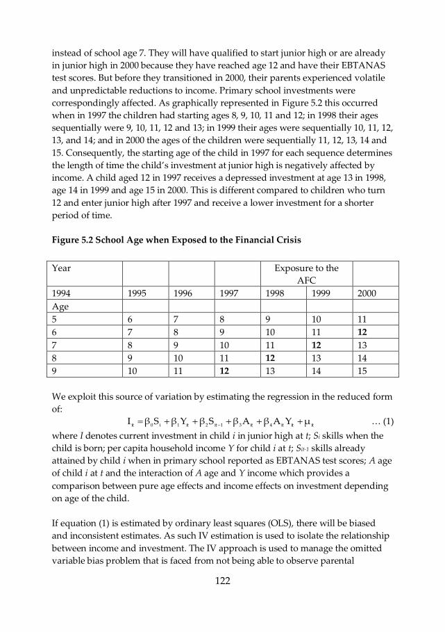
122

instead of school age 7. They will have qualified to start junior high or are already

in junior high in 2000 because they have reached age 12 and have their EBTANAS

test scores. But before they transitioned in 2000, their parents experienced volatile

and unpredictable reductions to income. Primary school investments were

correspondingly affected. As graphically represented in Figure 5.2 this occurred

when in 1997 the children had starting ages 8, 9, 10, 11 and 12; in 1998 their ages

sequentially were 9, 10, 11, 12 and 13; in 1999 their ages were sequentially 10, 11, 12,

13, and 14; and in 2000 the ages of the children were sequentially 11, 12, 13, 14 and

15. Consequently, the starting age of the child in 1997 for each sequence determines

the length of time the child’s investment at junior high is negatively affected by

income. A child aged 12 in 1997 receives a depressed investment at age 13 in 1998,

age 14 in 1999 and age 15 in 2000. This is different compared to children who turn

12 and enter junior high after 1997 and receive a lower investment for a shorter

period of time.

Figure 5.2 School Age when Exposed to the Financial Crisis

Year Exposure to the

AFC

1994 1995 1996 1997 1998 1999 2000

Age

5 6 7 8 9 10 11

6 7 8 9 10 11 12

7 8 9 10 11 12 13

8 9 10 11 12 13 14

9 10 11 12 13 14 15

We exploit this source of variation by estimating the regression in the reduced form

of:

ititit4it31it2it1i0it μYAβAβSβYβSβI

< (1)

where I denotes current investment in child i in junior high at t; Si skills when the

child is born; per capita household income Y for child i at t; Sit-1 skills already

attained by child i when in primary school reported as EBTANAS test scores; A age

of child i at t and the interaction of A age and Y income which provides a

comparison between pure age effects and income effects on investment depending

on age of the child.

If equation (1) is estimated by ordinary least squares (OLS), there will be biased

and inconsistent estimates. As such IV estimation is used to isolate the relationship

between income and investment. The IV approach is used to manage the omitted

variable bias problem that is faced from not being able to observe parental

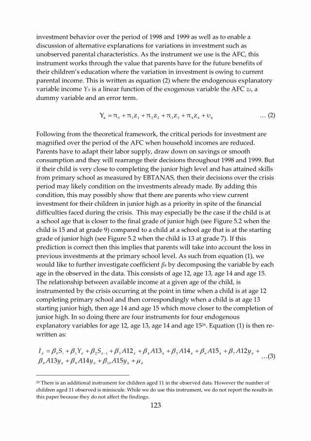
123

investment behavior over the period of 1998 and 1999 as well as to enable a

discussion of alternative explanations for variations in investment such as

unobserved parental characteristics. As the instrument we use is the AFC, this

instrument works through the value that parents have for the future benefits of

their children’s education where the variation in investment is owing to current

parental income. This is written as equation (2) where the endogenous explanatory

variable income Yit is a linear function of the exogenous variable the AFC z4, a

dummy variable and an error term.

it443322110it υzπzπzπzππY < (2)

Following from the theoretical framework, the critical periods for investment are

magnified over the period of the AFC when household incomes are reduced.

Parents have to adapt their labor supply, draw down on savings or smooth

consumption and they will rearrange their decisions throughout 1998 and 1999. But

if their child is very close to completing the junior high level and has attained skills

from primary school as measured by EBTANAS, then their decisions over the crisis

period may likely condition on the investments already made. By adding this

condition, this may possibly show that there are parents who view current

investment for their children in junior high as a priority in spite of the financial

difficulties faced during the crisis. This may especially be the case if the child is at

a school age that is closer to the final grade of junior high (see Figure 5.2 when the

child is 15 and at grade 9) compared to a child at a school age that is at the starting

grade of junior high (see Figure 5.2 when the child is 13 at grade 7). If this

prediction is correct then this implies that parents will take into account the loss in

previous investments at the primary school level. As such from equation (1), we

would like to further investigate coefficient β4 by decomposing the variable by each

age in the observed in the data. This consists of age 12, age 13, age 14 and age 15.

The relationship between available income at a given age of the child, is

instrumented by the crisis occurring at the point in time when a child is at age 12

completing primary school and then correspondingly when a child is at age 13

starting junior high, then age 14 and age 15 which move closer to the completion of

junior high. In so doing there are four instruments for four endogenous

explanatory variables for age 12, age 13, age 14 and age 1528. Equation (1) is then re-

written as:

itititit

itititititititiit

yAyAyA

yAAAAASYSI

151413

1215141312

1098

765431210<(3)

28 There is an additional instrument for children aged 11 in the observed data. However the number of

children aged 11 observed is miniscule. While we do use this instrument, we do not report the results in

this paper because they do not affect the findings.

<(3)

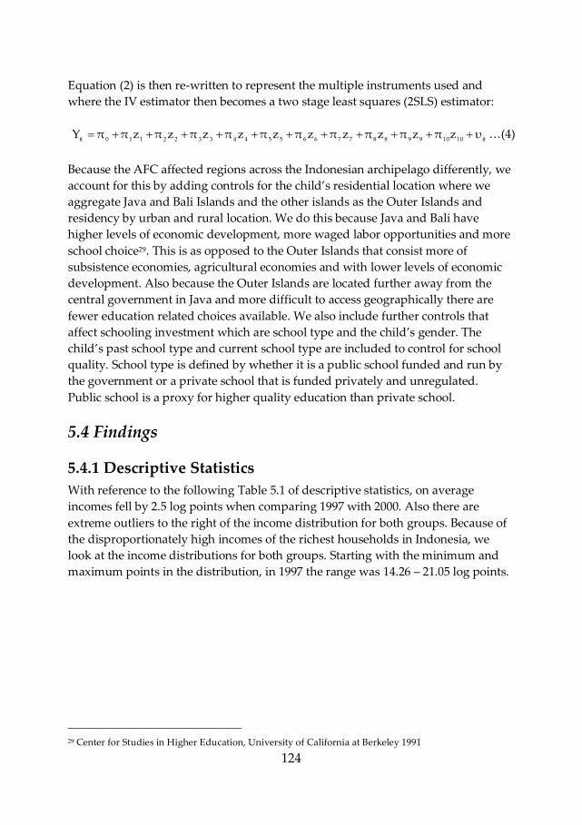
124

Equation (2) is then re-written to represent the multiple instruments used and

where the IV estimator then becomes a two stage least squares (2SLS) estimator:

it10109988776655443322110it υzπzπzπzπzπzπzπzπzπzππY <(4)

Because the AFC affected regions across the Indonesian archipelago differently, we

account for this by adding controls for the child’s residential location where we

aggregate Java and Bali Islands and the other islands as the Outer Islands and

residency by urban and rural location. We do this because Java and Bali have

higher levels of economic development, more waged labor opportunities and more

school choice29. This is as opposed to the Outer Islands that consist more of

subsistence economies, agricultural economies and with lower levels of economic

development. Also because the Outer Islands are located further away from the

central government in Java and more difficult to access geographically there are

fewer education related choices available. We also include further controls that

affect schooling investment which are school type and the child’s gender. The

child’s past school type and current school type are included to control for school

quality. School type is defined by whether it is a public school funded and run by

the government or a private school that is funded privately and unregulated.

Public school is a proxy for higher quality education than private school.

5.4 Findings

5.4.1 Descriptive Statistics

With reference to the following Table 5.1 of descriptive statistics, on average

incomes fell by 2.5 log points when comparing 1997 with 2000. Also there are

extreme outliers to the right of the income distribution for both groups. Because of

the disproportionately high incomes of the richest households in Indonesia, we

look at the income distributions for both groups. Starting with the minimum and

maximum points in the distribution, in 1997 the range was 14.26 – 21.05 log points.

29 Center for Studies in Higher Education, University of California at Berkeley 1991

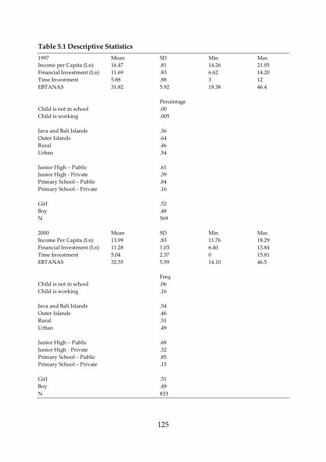
125

Table 5.1 Descriptive Statistics

1997 Mean SD Min Max

Income per Capita (Ln) 16.47 .81 14.26 21.05

Financial Investment (Ln) 11.69 .83 6.62 14.20

Time Investment 5.88 .88 3 12

EBTANAS 31.82 5.92 18.38 46.4

Percentage

Child is not in school .00

Child is working .005

Java and Bali Islands .36

Outer Islands .64

Rural .46

Urban .54

Junior High – Public .61

Junior High - Private .39

Primary School – Public .84

Primary School – Private .16

Girl .52

Boy .48

N 569

2000 Mean SD Min Max

Income Per Capita (Ln) 13.99 .83 11.76 18.29

Financial Investment (Ln) 11.28 1.03 6.40 13.84

Time Investment 5.04 2.37 0 15.81

EBTANAS 32.55 5.59 14.10 46.5

Freq

Child is not in school .06

Child is working .16

Java and Bali Islands .54

Outer Islands .46

Rural .51

Urban .49

Junior High – Public .68

Junior High - Private .32

Primary School – Public .85

Primary School – Private .15

Girl .51

Boy .49

N 833

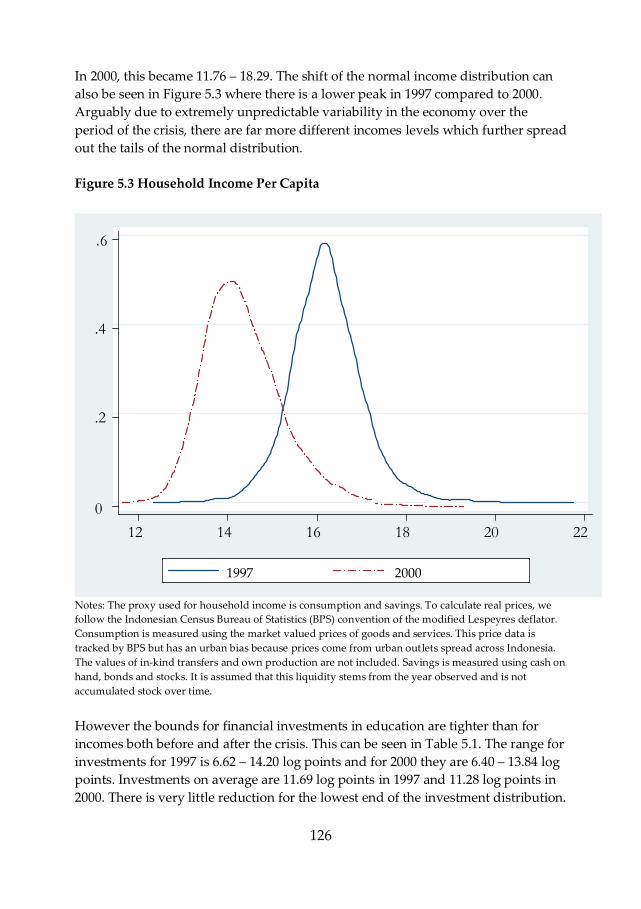
126

In 2000, this became 11.76 – 18.29. The shift of the normal income distribution can

also be seen in Figure 5.3 where there is a lower peak in 1997 compared to 2000.

Arguably due to extremely unpredictable variability in the economy over the

period of the crisis, there are far more different incomes levels which further spread

out the tails of the normal distribution.

Figure 5.3 Household Income Per Capita

Notes: The proxy used for household income is consumption and savings. To calculate real prices, we

follow the Indonesian Census Bureau of Statistics (BPS) convention of the modified Lespeyres deflator.

Consumption is measured using the market valued prices of goods and services. This price data is

tracked by BPS but has an urban bias because prices come from urban outlets spread across Indonesia.

The values of in-kind transfers and own production are not included. Savings is measured using cash on

hand, bonds and stocks. It is assumed that this liquidity stems from the year observed and is not

accumulated stock over time.

However the bounds for financial investments in education are tighter than for

incomes both before and after the crisis. This can be seen in Table 5.1. The range for

investments for 1997 is 6.62 – 14.20 log points and for 2000 they are 6.40 – 13.84 log

points. Investments on average are 11.69 log points in 1997 and 11.28 log points in

2000. There is very little reduction for the lowest end of the investment distribution.

0

.2

.4

.6

12 14 16 18 20 22

1997 2000

127

The fall in investment is primarily coming from the highest 20% of households of

the income distribution.

Looking at the other specification for investment which is the amount of schooling

time allocated we also find a reduction in 2000. On average time spent in school

each day fell from 5.88 hours in 1997 to 5.04 hours in 2000. For both periods, this

average time amount is below the required 7.6 hours based on the national

academic curriculum. The range of schooling time in 1997 was 3 – 12 hours per day.

In contrast, the range for 2000 was spread out to 0 – 15.81 hours per day with

greater variability compared to 1997.

The schooling time distributions also show that the 6th percentile of children in 1997

reported zero hours allocated for schooling. In addition 0.16 of the 2000 sample

reported working. The ages of the 0.16 of this 2000 sample are 14 and 15. In

comparison, no children in the 1997 group reported 0 hours of schooling. We

interpret this to mean that for the 0.06 not in school, they may either be at home or

working; or at home and working. Since the percentage of children reporting

working status is higher than the percentage of children with zero hours in school,

this suggests that there are children simultaneously working and going to school in

200030. We will investigate time investments further in the next section using IV

analysis. When we do this, we will transform the variable into log terms to enable

ease of comparison.

Despite an income reduction, the children’s stock of skill was not severely affected.

From the descriptive statistics in Table 5.1, it can be seen that average test scores

were higher in 2000. On average test scores in 2000 were 32.55 points in contrast to

31.82 points in 1997. But the minimum for scores in 2000 is an extremely low 14.10

points compared to 18.38 points in 1997. For children in the lower end of the

EBTANAS standardized test score distribution, more of them failed almost all of

the five subjects tested over the period of the crisis, all of 1998, 1999 and most of

2000. The lowest performance in 2000 versus 1997 came from the science test (this

statistic is not reported). The best performance for the children in the lower end of

the score distribution in 2000 against 1997 is the Indonesian language literacy test.

Looking at the highest end of the test score distribution, there is no change for both

groups. Children in the lower end of the EBTANAS distribution are pulling down

performance while the achievements of the children from the median to the top 1%

of the distribution remained unchanged. More importantly, the distribution of

skills in both periods appears to be a result of selection bias. It seems that the

children with test scores higher than the median score in both groups have the

same stock of skills. But the children selected into the group in 2000 with lower

30 I investigate simultaneous work-schooling behavior in Chapter 4.

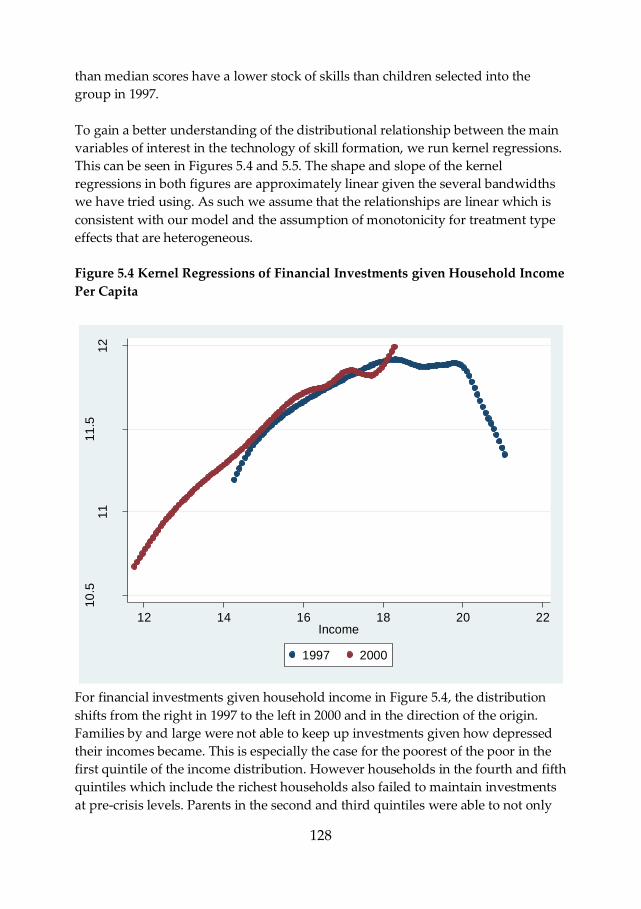
128

than median scores have a lower stock of skills than children selected into the

group in 1997.

To gain a better understanding of the distributional relationship between the main

variables of interest in the technology of skill formation, we run kernel regressions.

This can be seen in Figures 5.4 and 5.5. The shape and slope of the kernel

regressions in both figures are approximately linear given the several bandwidths

we have tried using. As such we assume that the relationships are linear which is

consistent with our model and the assumption of monotonicity for treatment type

effects that are heterogeneous.

Figure 5.4 Kernel Regressions of Financial Investments given Household Income

Per Capita

10

.511

11

.512

Edu

catio

na

l In

vestm

ents

12 14 16 18 20 22Income

1997 2000

For financial investments given household income in Figure 5.4, the distribution

shifts from the right in 1997 to the left in 2000 and in the direction of the origin.

Families by and large were not able to keep up investments given how depressed

their incomes became. This is especially the case for the poorest of the poor in the

first quintile of the income distribution. However households in the fourth and fifth

quintiles which include the richest households also failed to maintain investments

at pre-crisis levels. Parents in the second and third quintiles were able to not only

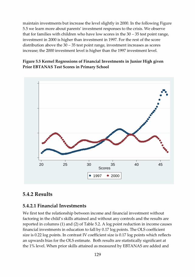
129

maintain investments but increase the level slightly in 2000. In the following Figure

5.5 we learn more about parents’ investment responses to the crisis. We observe

that for families with children who have low scores in the 30 – 35 test point range,

investment in 2000 is higher than investment in 1997. For the rest of the score

distribution above the 30 – 35 test point range, investment increases as scores

increase; the 2000 investment level is higher than the 1997 investment level.

Figure 5.5 Kernel Regressions of Financial Investments in Junior High given

Prior EBTANAS Test Scores in Primary School

100

00

02

00

00

03

00

00

04

00

00

0

Ed

uca

tion

al In

ve

stm

ents

20 25 30 35 40 45Scores

1997 2000

5.4.2 Results

5.4.2.1 Financial Investments

We first test the relationship between income and financial investment without

factoring in the child’s skills attained and without any controls and the results are

reported in columns (1) and (2) of Table 5.2. A log point reduction in income causes

financial investments in education to fall by 0.17 log points. The OLS coefficient

size is 0.22 log points. In contrast IV coefficient size is 0.17 log points which reflects

an upwards bias for the OLS estimate. Both results are statistically significant at

the 1% level. When prior skills attained as measured by EBTANAS are added and

130

this is seen in specifications (3) – (10), the magnitude of the income coefficient

remains at approximately 0.20 for OLS and at 0.17 for IV and is statistically

significant at the 1% level. These estimates remain unaffected by the introduction of

control variables. The IV estimates across specifications (1) – (10) indicate that the

OLS estimates are biased upwards for unobserved reasons. This finding then

strongly implies that in the presence of income constraints, 80% of the cross-

sectional link between income and financial investment in education is caused by

differences in income. The remaining 20% of the cross-sectional link between

income and educational investment is caused by differences in parental

characteristics.

When the stock of skills variable is included as a specification in (3) and (4), we find

that prior skills attained have a smaller relationship with investment compared to

the causal relationship between income and investment. A one test point increase

in EBTANAS increases educational expenditures by 0.02 log points; this is for both

the OLS and IV estimates and is statistically significant at the 1% level. It appears

that the differences in the observed human capital accumulated earlier in primary

school explain very little for later investment. When the control variables Java and

Bali residency, urban residency, school type and gender are added in specifications

(5) and (6), the impact of skills attained on investment weakens to 0.01 log points.

Statistical significance falls to the 5% level. This suggests that differences in where

the child resides and goes to school and gender differences further weaken the

relationship between stock of skills and investment. From these results, we show

that 0.8 of the cross-sectional link between income and educational expenditures

are caused by differences in income and this result is robust across specifications

(1) – (10).

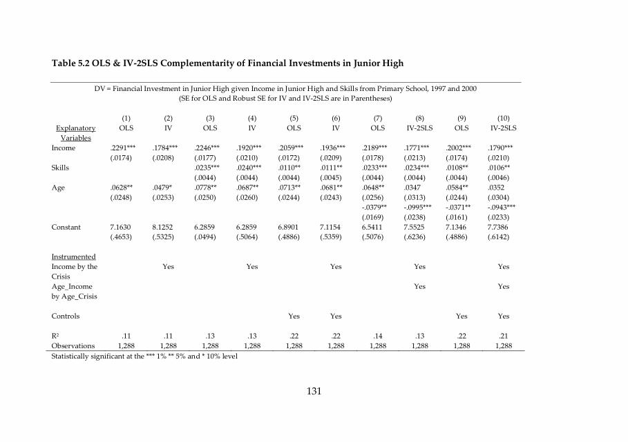
131

Table 5.2 OLS & IV-2SLS Complementarity of Financial Investments in Junior High

DV = Financial Investment in Junior High given Income in Junior High and Skills from Primary School, 1997 and 2000

(SE for OLS and Robust SE for IV and IV-2SLS are in Parentheses)

(1) (2) (3) (4) (5) (6) (7) (8) (9) (10)

Explanatory

Variables

OLS IV OLS IV OLS IV OLS IV-2SLS OLS IV-2SLS

Income .2291***

(.0174)

.1784***

(.0208)

.2246***

(.0177)

.1920***

(.0210)

.2059***

(.0172)

.1936***

(.0209)

.2189***

(.0178)

.1771***

(.0213)

.2002***

(.0174)

.1790***

(.0210)

Skills .0235***

(.0044)

.0240***

(.0044)

.0110**

(.0044)

.0111**

(.0045)

.0233***

(.0044)

.0234***

(.0044)

.0108**

(.0044)

.0106**

(.0046)

Age .0628**

(.0248)

.0479*

(.0253)

.0778**

(.0250)

.0687**

(.0260)

.0713**

(.0244)

.0681**

(.0243)

.0648**

(.0256)

.0347

(.0313)

.0584**

(.0244)

.0352

(.0304)

-.0379**

(.0169)

-.0995***

(.0238)

-.0371**

(.0161)

-.0943***

(.0233)

Constant 7.1630

(.4653)

8.1252

(.5325)

6.2859

(.0494)

6.2859

(.5064)

6.8901

(.4886)

7.1154

(.5359)

6.5411

(.5076)

7.5525

(.6236)

7.1346

(.4886)

7.7386

(.6142)

Instrumented

Income by the

Crisis

Yes Yes Yes Yes Yes

Age_Income

by Age_Crisis

Yes Yes

Controls Yes Yes Yes Yes

R2 .11 .11 .13 .13 .22 .22 .14 .13 .22 .21

Observations 1,288 1,288 1,288 1,288 1,288 1,288 1,288 1,288 1,288 1,288

Statistically significant at the *** 1% ** 5% and * 10% level

132

Notes: The age range is from 11 – 15. For the interaction of age and income, the age variable has been de-

meaned and the income variable has been de-meaned. The control variables are if the child resides and

goes to school in the Java and Bali Islands; if the child is in an urban area; the child’s school type at the

primary school level and junior high level and if the child is a girl or boy.

In columns (7) and (8) of Table 5.3, we introduce the OLS estimates for comparison

with the 2SLS estimates. We instrument income by the crisis and instrument the

interaction of age and available income by age and the crisis and without controls.

The OLS and 2SLS estimates for income are the same as the prior specifications and

are robust. The skill variable is now increased back to 0.02 log points and

statistically significant at the 1% level. But we find that the interaction of age with

income has a negative causal relationship with educational expenditures. In

response to a reduction in income, parents increase financial investment by 0.03 log

points when the child is older by a year. The coefficient size for the 2SLS estimate is

a smaller 0.09 which indicates that the OLS estimate is biased downwards for

unobserved reasons. This result is statistically significant for the 2SLS estimate at

the 1% level compared to the statistical significance for the OLS estimate at the 5%

level. When controls are re-introduced, the results as can be seen in specifications

(9) and (10) remain similar to specifications (7) and (8). The exception is that the

size of the skills coefficient is reduced by half again where a one test point increase

in EBTANAS only raises investment by 0.01 log points instead of 0.02 log points.

As the sensitive time in our model (Section 5.2) is the period of junior high at t = 2

after the child has completed and transitioned from primary school at t = 1, we

proceed to detail which school ages within the junior high level are investment

priorities. The relationship between available income at a given age of the child, is

instrumented by the crisis occurring at the point in time when a child is at age 12

completing primary school and then correspondingly when a child is at age 13

starting junior high, then age 14 and age 15 which move closer to the completion of

junior high and the beginning of the minimum legal employment age. The OLS and

2SLS results are presented in Table 5.3 and the coefficient sizes are similar across all

specifications (11) – (14).

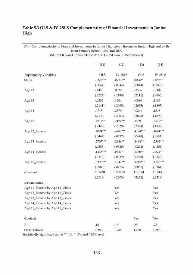
133

Table 5.3 OLS & IV-2SLS Complementarity of Financial Investments in Junior

High

DV = Complementarity of Financial Investments in Junior High given Income in Junior High and Skills

from Primary School, 1997 and 2000

(SE for OLS and Robust SE for IV and IV-2SLS are in Parentheses)

(11) (12) (13) (14)

Explanatory Variables OLS IV-2SLS OLS IV-2SLS

Skills .0223*** .0223*** .0096** .0095**

(.0044) (.0044) (.0044) (.0045)

Age 12 -.1450 .0027 -.2536 -.0902

(.2224) (.2180) (.2111) (.2066)

Age 13 -.0335 .1504 -.0880 .1165

(.2141) (.2005) (.2035) (.1893)

Age 14 .0718 .2579 -.0241 .1818

(.2133) (.2003) (.2028) (.1896)

Age 15 .4917** .7124*** .3489 .6512**

(.2442) (.2028) (.2324) (.1932)

Age 12_Income .4094*** .4702*** .4124*** .4841***

(.0464) (.0657) (.0440) (.0631)

Age 13_Income .2707*** .2446*** .2464*** .2302***

(.0305) (.0320) (.0292) (.0304)

Age 14_Income .1438*** .0621* .1350*** .0824**

(.0272) (.0339) (.0260) (.0323)

Age 15_Income .3998*** .4342*** .3245*** .4146***

(.0908) (.0275) (.0865) (.0361)

Constant 10.6991 10.5159 11.0174 10.8150

(.2518) (.2405) (.2442) (.2318)

Instrumented

Age 11_Income by Age 11_Crisis Yes Yes

Age 12_Income by Age 12_Crisis Yes Yes

Age 13_Income by Age 13_Crisis Yes Yes

Age 14_Income by Age 14_Crisis Yes Yes

Age 15_Income by Age 15_Crisis Yes Yes

Controls Yes Yes

R2 .16 .15 .25 .25

Observations 1,288 1,288 1,288 1,288

Statistically significant at the *** 1%, ** 5% and * 10% level

134

Notes: The age range is from 11 – 15. The reference age group is 11. The results for age 11 (not reported)

have a miniscule effect on the coefficient size for financial investments. For the interaction of each age

and income, the variable for each age is represented by a dummy and the income variable has been de-

meaned. The control variables are if the child resides and goes to school in the Java and Bali Islands; if

the child is in an urban area; the child’s school type at the primary school level and junior high level and

if the child is a girl or boy.

When the child is aged 12, has completed EBTANAS for primary school and given

an income reduction investment falls by 0.4. This decrease in investment at age 12

may perhaps be partly explained by government subsidies offsetting parental

spending in order to ensure that children complete the final grade of primary

school. But when the child is older by a year at age 13, has started junior high at

grade 7 and given an income reduction, investment only falls by 0.2. When the

child is aged 14, a year prior to taking EBTANAS for junior high to enter senior

high; and a year prior to being old enough to enter the labor force, an income

reduction causes investment to decrease by only 0.08. At age 15, an income

decrease causes a larger decrease in investment of 0.3 for OLS and 0.4 for 2SLS.

This implies that the 0.3 of the link between income and investment at age 15 is

caused by income and 0.7 by unobserved factors. This substantial decrease in

investment at age 15 then implies that investment decision making is influenced by

a new set of factors. There is now a fork in the decision path where the child can

either take EBTANAS to transition to senior high or take EBTANAS then enter the

labor force at the legal minimum age of 15. The presence of two options – to

continue with higher education or to work is consistent with the descriptive

statistics where for ages 14 and 15 in the 2000 sample 0.06 of the children reported

zero hours allocated for formal schooling and 0.16 reported working. In contrast no

children of the same age in the 1997 sample reported zero formal schooling time

and 0.005 of the children worked.

The pattern of reduction in educational expenditures is much lower for children

who have already attained a few years of junior high education. The reduction is

lower for the child aged 14 than for the child aged 13 and both have reductions

lower than for the child aged 12 who has only attained a primary school education.

This means that junior high investments are a priority despite depressed household

incomes. This implies that parents do take into account the loss in returns related to

previous investments on the stock of human capital accumulated. But this

investment behavior appears to only be partly explained up to 0.8 by differences in

household income related characteristics. The remaining 0.2 explanation for this

pattern of investment is related to parental characteristics such as scholastically

motivated parents. Such parents may view education as a high priority in their

children’s lifecycle. They allocate more of their children’s time for formal schooling

and do not consider the possibility of their children working or helping in the

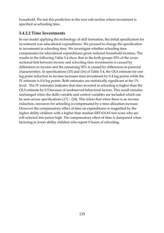
135

household. We test this prediction in the next sub-section where investment is

specified as schooling time.

5.4.2.2 Time Investments

In our model applying the technology of skill formation, the initial specification for

investment was educational expenditures. We proceed to change the specification

to investment in schooling time. We investigate whether schooling time

compensates for educational expenditures given reduced household incomes. The

results in the following Table 5.4 show that in the both groups 50% of the cross-

sectional link between income and schooling time investments is caused by

differences in income and the remaining 50% is caused by differences in parental

characteristics. In specifications (15) and (16) of Table 5.4, the OLS estimate for one

log point reduction in income increases time investment by 0.4 log points while the

IV estimate is 0.6 log points. Both estimates are statistically significant at the 1%

level. The IV estimates indicates that time invested in schooling is higher than the

OLS estimate by 0.5 because of unobserved behavioral factors. This result remains

unchanged when the skills variable and control variables are included which can

be seen across specifications (17) – (24). This infers that when there is an income

reduction, resources for schooling is compensated by a time allocation increase.

However the compensatory effect of time on expenditures is magnified by the

higher ability children with a higher than median EBTANAS test score who are

self-selected into junior high. The compensatory effect of time is dampened when

factoring in lower ability children who report 0 hours of schooling.

136

Table 5.4 OLS & IV-2SLS Complementarity of Time Investments in Junior High

DV = Complementarity of Time Investments in Junior High given Income in Junior High and Skills from Primary School, 1997 and 2000

(SE for OLS and Robust SE for IV and IV-2SLS are in Parentheses)

(15) (16) (17) (18) (19) (20) (21) (22) (23) (24)

Explanatory

Variables

OLS IV OLS IV OLS IV OLS IV-2SLS OLS IV-2SLS

Income -.4097***

(.0121)

-.6047***

(.0147)

-.4151***

(.0124)

-.5961***

(.0147)

-.4187***

(.0127)

-.6030***

(.0152)

-.4151***

(.0124)

-.5919***

(.0144)

-.4187***

(.0127)

-.5988***

(.0150)

Skills .0249***

(.0031)

.0270***

(.0033)

.0215***

(.0033)

.0231***

(.0034)

.0249***

(.0031)

.0271***

(.0033)

.0215***

(.0033)

.0231***

(.0034)

Age -.0205

(.0173)

-.0380**

(.0177)

.0345*

(.0179)

-.0237

(.0203)

.0353**

(.0179)

-.0210

(.0201)

.0345*

(.0179)

-.0140

(.0184)

.0353**

(.0179)

-.0111

(.0181)

Age_Income -.0011

(.0118)

.0040

(.0147)

-.0006

(.0118)

.0040

(.0145)

Constant 8.5062

(.3253)

12.2261

(.3587)

7.6013

(.3565)

11.0252

(.4122)

76.773

(.3599)

11.1474

(.4105)

7.6013

(.3565)

10.8387

(.3800)

7.6773

(.3599)

10.9669

(.3790)

Instrumented

Income by the

Crisis

Yes Yes Yes Yes Yes

Age_Income

by Age_Crisis

Yes Yes

Controls Yes Yes Yes Yes

R2 .47 .39 .49 .37 .50 .41 .49 .41 .50 .42

Observations 1,348 1,348 1,271 1,271 1,271 1,271 1,271 1,271 1,271 1,271

Statistically significant at the *** 1%, ** 5% and * 10% level

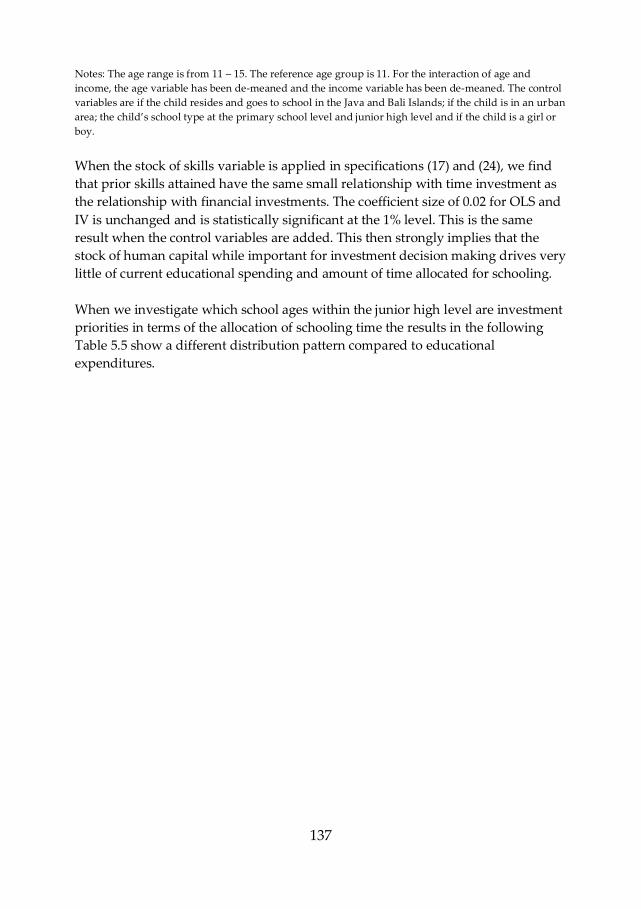
137

Notes: The age range is from 11 – 15. The reference age group is 11. For the interaction of age and

income, the age variable has been de-meaned and the income variable has been de-meaned. The control

variables are if the child resides and goes to school in the Java and Bali Islands; if the child is in an urban

area; the child’s school type at the primary school level and junior high level and if the child is a girl or

boy.

When the stock of skills variable is applied in specifications (17) and (24), we find

that prior skills attained have the same small relationship with time investment as

the relationship with financial investments. The coefficient size of 0.02 for OLS and

IV is unchanged and is statistically significant at the 1% level. This is the same

result when the control variables are added. This then strongly implies that the

stock of human capital while important for investment decision making drives very

little of current educational spending and amount of time allocated for schooling.

When we investigate which school ages within the junior high level are investment

priorities in terms of the allocation of schooling time the results in the following

Table 5.5 show a different distribution pattern compared to educational

expenditures.

138

Table 5.5 OLS & IV-2SLS Complementarity of Time investments in Junior High

DV = Complementarity of Time Investments in Junior High given Income in Junior

High and Skills from Primary School, 1997 and 2000

(SE for OLS and Robust SE for IV and IV-2SLS are in Parentheses)

(25) (26) (27) (28)

Explanatory Variables OLS IV-2SLS OLS IV-2SLS

Skills .0243*** .0268*** .0213*** .0233***

(.0031) (.0033) (.0033) (.0034)

Age 12 .1828 .1432 .1699 .1165

(.1621) (.2047) (.1620) (.2111)

Age 13 .1709 .0196 .1683 .0144

(.1567) (.1967) (.1567) (.2026)

Age 14 .2463 .0945 .2384 .0829

(.1561) (.1967) (.1562) (.2031)

Age 15 .5504** .1205 .5464 .1152

(.1771) (.2094) (.1775) (.2132)

Age 12_Income -.4067*** -.6231*** -.4039*** -.6234***

(.0323) (.0448) (.0323) (.0445)

Age 13_Income -.4448*** -.5968*** -.4472*** -.6034***

(.0214) (.0240) (.0215) (.0242)

Age 14_Income -.4171*** -.5993*** -.4196*** -.6050***

(.0190) (.0239) (.0192) (.0242)

Age 15_Income -.2268*** -.4726*** -.2334*** -.4863***

(.0628) (.0620) (.0631) (.0564)

Constant 1.6334 1.7149 1.6653 1.772

(.1837) (.2218) (.1873) (.2308)

Instrumented

Age 11_Income by Age 11_Crisis Yes Yes

Age 12_Income by Age 12_Crisis Yes Yes

Age 13_Income by Age 13_Crisis Yes Yes

Age 14_Income by Age 14_Crisis Yes Yes

Age 15_Income by Age 15_Crisis Yes Yes

Control Variables Yes Yes

R2 .50 .42 .51 .43

Observations 1,271 1,271 1,271 1,271 Statistically significant at the *** 1%, ** 5% and * 10% level

139

Notes: The age range is from 11 – 15. The reference age group is 11. The results for age 11 (not reported)

have a miniscule effect on the coefficient size for financial investments. For the interaction of each age

and income, the variable for each age is represented by a dummy and the income variable has been de-

meaned. The control variables are if the child resides and goes to school in the Java and Bali Islands; if

the child is in an urban area; the child’s school type at the primary school level and junior high level and

if the child is a girl or boy.

The interaction of each age 12, 13, 14 and 15 with income as instrumented by each

age with the crisis show that time investment is uniformly increased across age 12,

age 13 and 14. For each additional year of the child’s age given an income reduction

but only up to age 14, time investment increases by approximately 0.4 log points

for OLS and 0.6 log points for 2SLS. This is statistically significant at the 1% level.

These coefficient magnitudes hold with and without control variables as can be

seen in specifications (25) – (28) in Table 5.5. Given the difference between 0.4 for

the OLS estimate and 0.6 for the 2SLS estimate, it is strongly inferred that 50% of

the cross-sectional link between schooling time investments at age 12, age 13 and 14

and available income are caused by differences in income. The remaining 50% of

the cross-sectional link is caused by differences in parental characteristics or

differences in child characteristics. This suggests that there are parents who favor

education and are less inclined for their children aged 12 – 14 to allocate time for

work or helping in the household. Likewise the children may be scholastically

motivated and are more likely to spend more time studying. But the inclination to

be in school more hours may be limited to high quality and affordable public

schools. However there is a threshold at age 15 when time investment decision

making changes. The OLS estimate reduces to 0.2 log points and the 2SLS estimate

reduces to 0.4 log points and both are statistically significant at the 1% level.

Schooling time compensates less for educational expenditures at age 15 compared

to ages 12 – 14 but the differences explaining for this remain as half for income and

half for unobserved parental characteristics. This is reflected by 0.16 of the 2000

group dividing time between schooling and working. Also this investment

behavior may perhaps be attributed to the two choices that a 15 year old has –

complete junior high and go on to senior high or complete junior high and enter the

labor force.

5.5 Conclusions Optimal parental investments in education depend on an evaluation of upfront

costs and delayed benefits. If education was only viewed as a consumption good,

income would determine optimal investments. In the Indonesian context of

incomplete credit markets, we find that there is a causal interpretation between

reduced income and financial investments in education. Using repeated cross

sections from 1997 and 2000, 80% of the cross sectional link between income and

educational spending is caused by differences in income. The remaining 20% is

140

caused by unobserved parental characteristics or unobserved child characteristics.

Our findings also show that the 50% of cross sectional link between income and

time investment in education is caused by differences in income. Financial

investments and time investments in education compensate for each other when

household income is reduced. But this appears to only be for higher ability children

who have completed primary school and selected to enter junior high. This does

not appear to be the case for lower ability children in junior high where educational

expenditures and schooling time do not compensate each other.

This chapter has also shown that due to the dynamic complementarity of skills

attained the reduction in educational expenditures is much lower for children who

have already attained a few years of junior high education. This implies that

parents do take into account the loss in returns related to previous investments on

the stock of human capital accumulated. Put another way, parents do face a loss

aversion where sunk costs do matter. But at age 15 the final year of junior high and

the minimum legal age for employment, the reduction in expenditures is far greater

than for the earlier grades of junior high. This suggests that the child may enter the

labor force and have earning opportunities that match the skills accumulated up to

junior high. As households bear up to 60% of the total educational cost, low income

households may assess that going on to senior high may entail costs that far

outweigh market earning opportunities. As pointed out in the literature on

educational investment in developing countries, parents may view the market

value of schooling up to a certain school level and in the context of Indonesia this

may possibly be at junior high. Hence for low income households, educational

investments may then be sub-optimal.

The conclusions that we draw here is that monetary constraints drive schooling

decisions for Indonesian children at the junior high level. This is not the case at the

primary school level which is heavily subsidized by central and regional

government. Parents make sub-optimal investments when they equate the direct

and opportunity costs of education with future benefits up to only the junior high

level and not at higher levels of education. However, there are parents with

children of higher ability who are favorably pre-disposed to higher education

where they make investments in both time and money. The parents who are

scholastically motivated are then inclined for their children to go on to higher

levels of education. But for lower income households with lower ability children,

junior high becomes the level at which children may end up working pre-maturely

instead of gaining more education. The longer term consequence is then that in

adulthood they will have a lower stock of human capital and will be unable to

compete in the labor market against others with higher ability and higher

education levels.

141

6. Main Findings and Implications

142

6.1 Main Findings

Education is considered to be very important for economic growth. But family

investments in education are much lower in developing countries compared to

developed countries. This leads to the question whether families in developing

countries have a low preference to invest and whether the market rates of return

are very low; or that there are actually constraints to investment.

The aim of this dissertation has been to investigate whether families in developing

countries face actual constraints to investing in their children’s human capital.

Empirically we have determined two main constraints to educational investment in

the Indonesian developing country context: resource constraints on basic facilities –

we used the access to and use of electricity for studying; and monetary constraints

as captured by family income. This empirical work is covered in four chapters. The

method that we have used to determine these two main constraints on investment

in basic education is the natural experiment or a comparative method focusing on

Indonesian families over two periods, 1997 and 2000 where the Asian Financial

Crisis occurred in 1998 and 1999.

The main findings in Chapter 2 are that in response to an income reduction,

families used various ways to ensure that their children continued their education

in primary school and junior high. Parents’ adaptive strategies were to shift their

children from high quality formal education to low quality non-formal and

informal school; maintained a scheduled monthly flow of fees / contributions to

keep the school operational or risk their children being withheld from school;

trading off timely monthly flow payments by reducing spending on school

expenditures at the intensive margin such as school uniforms and sports

equipment; and only high ability children on the basis of test scores were selected

to transition from formal primary school to formal junior high. An additional

finding is that there are regional geographical patterns to the different school types

that children attended before and after the Asian Financial Crisis.

In Chapter 3, the main findings stem from investigating the regional patterns in

schooling across the Indonesian archipelago. 12 year old children who have more

access to electricity have better educational performance. The potential pathway

between the availability of electricity and test score performance is via how

children use electricity in school and in the household to improve learning

efficiency. However given the fixed placement of the national electricity grid which

pre-dominates in Java and Bali Islands, children in economically developed areas

have higher test score performance than disadvantaged children in

143

underdeveloped, lagging behind areas. The regional distribution of electricity is an

inherent resource constraint for schooling and learning. The lack of access to

electricity is viewed as a non-monetary resource constraint on education as family

income has a minimal influence on how the state distributes electricity.

The main findings in Chapter 4 are that there are children who are pre-disposed to

working from as young as age 6 and then starting to attend school and they

continue to work more as they become older. Work manifests itself in terms of

working within the household for the family (e.g. household chores or farm work)

or outside of the household for wages or in-kind transfers. Children especially boys

work more hours outside the household and for wages when they are older than

12. We find that simultaneous work-schooling behavior does not interrupt

schooling and does not impair human capital accumulation as much as would have

been expected. However child workers who attend non-formal school with flexible

hours that cater to their work patterns; and children who work as family

apprentices have lower qualifications than children in the formal education system.

This increases the probability of poor formal labor market outcomes later in life.

But child apprentices appear to be able to continue the traditional family trade

which may be viewed as having a high social return.

In Chapter 5, the main findings are that there exists a relationship between family

income and educational investment in Indonesia. A reduction in family income

reduces the amount used to finance schooling in junior high but this is

compensated by an increase in the amount of time invested in schooling and

learning. Despite reduced incomes, the family is not likely to terminate schooling

and this is as described in Chapter 2. Optimal education investment does include

accounting for the loss in returns from previous investments on the stock of human

capital that has been accumulated. Put another way, parents do face a loss aversion

where sunk costs do matter. Using repeated cross sections from 1997 and 2000, we

find that about 80% of the cross-sectional link between income and educational

expenditures is caused by differences in income. The remaining 20% is related to

unobserved parental characteristics. Strong influences for complementing prior

educational investment are when the child is close to completing junior high as

opposed to having just started junior high; and when the child has high cognitive

ability on the basis of prior primary school test scores.

6.2 Implications

The central finding of this dissertation is that families in developing countries do

not have a lower preference for education; but rather they are confronted with

resource constraints – the lack of school quality; and income constraints. Because

144

families are constrained, we will argue that policymakers can look at different ways

apart from educational financing and the formal educational system to increase

human capital. It is our position that understanding the social and economic status

of individual families and the constraints they face plays an important role in

educational policymaking.

Developing country governments tend to intervene in the provision of education

by building more schools, increasing the number of qualified teachers and

providing scholarships to disadvantaged children. Yet in the Indonesian context,

since 1997 when the Asian Financial Crisis occurred, the percentage of children

who complete a full course of 9 years of primary school and junior high has

steadily fallen from 75% in 1997 to 52.6% in 2001. Because of the main constraints to

educational investment, we posit that different families by social and economic

status have a different calculus of decision making. While in normative terms,

parental financing of education is meant to improve the child’s labor market

outcomes in adulthood, developing country families consider far more factors. The

calculus of decision making is most likely not about progressing from one school

grade to another. Instead the factors under consideration are concerned with

progressing from one school level to another. Given the evidence provided in this

dissertation, these factors are regional geographical constraints on school quality;

joint work-schooling starting from age 6 until age 15 at the end of junior high when

they can legally enter the labor market fulltime; and whether the children have the

cognitive skills to merit investment in education in senior high and university.

While near universal primary school education has been achieved, we posit that if

there is a clear understanding of the factors and constraints that families face when

their children are about to transition from primary school to junior high, there is a

higher likelihood that they will achieve all 3 years of schooling at junior high. That

is, the battleground to be fought for achieving 9 years of universal basic education

is at the junior high level. The battleground is no longer at the primary school level.

The school resource constraints and income constraints are likely to be tightest

when the child is aged 12 – 15. If the child has attended 6 years of primary school in

an underdeveloped, lagging behind village with only basic infrastructure, the

family may choose for the child to drop out. The school and home environment

may not be conducive for continued education at the junior high level. If a child

who is accustomed to working since age 6 and has turned 12 after completing

primary school, the child may be more likely to work more and attend school less.

This is because the child especially a boy working in an urban area may have a

higher relative value of time for working rather than attend a low quality school,

learning little. But there is evidence that once a child has started a few years of

junior high through ages 13 and 14, parents are more likely to continue financing

the child’s education until junior high is completed. By concentrating on the

145

educational choices that families make during this at risk period of three years of

junior high, policymakers are likely to be more successful in increasing schooling

attainment.

There are various concrete ways to relax these constraints on educational

investment. The resource constraint on basic facilities such as electricity access can

be relaxed when the state increases the distribution of electricity for school and

household use. This will mean redistributing energy capacity away from industrial

and transport use. This can be carried out as a part of the country’s redistribution

program that reduces not just income inequality but schooling inequalities. The

family income constraint can be less tight when the state disproportionately

increases student scholarships and expenditures for junior high schools when the

child is aged 13 in grade 8 and aged 14 in grade 9. Since there is evidence that

families substitute lower educational expenditures with higher time allocated for

studying, increasing electricity access in the school and household increases the

number of hours that a child can choose to use for learning activity. Hence, it is

possible to cogitate that educational investment constraints may interact and that

relaxing one loosens the other constraints.

Because of unobserved ability that may perhaps include less scholastic motivation,

there will be children who are less likely to complete a full course of 9 years of basic

education in the formal education system. These are children who are child

workers or apprentices who have gained marketable skills from young by learning

on the job. There is evidence of children who self-select out of the formal education

system and opt for non-formal and informal schooling. For this group of children,

school resource constraints and income constraints may not be the main factors

restricting decision making. Their families may view their children’s relative value

of time to be higher in market work and household production compared to formal

schooling. By recognizing these family perspectives, educational policymakers

particularly in Indonesia should continue to expand on non-formal and informal

schooling choices for this group of children. Based on our knowledge, Indonesia is

the only developing country in the world to have a national educational system

that provides schooling alternatives for child workers. These schooling alternatives

guarantee that economically active children receive some form of schooling

regardless of whether they work by choice or because they are forced to. As akin to

the Coleman Report and arguments made by Heckman and Lochner (1999), our

position is about rethinking how education and training can be used to build

socially productive skills and not just marketable skills in the formal sector. For

example, a child apprentice from a fishing family in Indonesia may be able to carry

on with the family tradition passing skills from one generation to another. This

tradition may perhaps be protected when the child receives modern technical skills

training to complement existing skills learnt on the job.

146

In forthcoming work, we will reconcile the educational choices of children in the

formal and alternative schools and examine their longer term educational and labor

market outcomes. New available IFLS data in 2007 will enable us to investigate

how family decision making over the period of the Asian Financial Crisis affects

later outcomes. While the effects of the financial crisis washed away relatively

quickly at the macroeconomic level, we would like to investigate if there are longer

term consequences in the labor market and within society.

147

Bibliography

Alatas, Vivi (2000) “Evaluating the Left Behind Villages Program in Indonesia:

Exploiting Rules to Identify Effects on Employment and Expenditures” Ph. D.

thesis, Princeton University

Aguiar, Mark and Hurst, Erik (2005) “Consumption vs. Expenditure” Journal of

Political Economy 113:5, pp. 919 – 948

Bacalod, Marigee P. and Tobias, Justin L. “School, School Quality and Achievement

Growth: Evidence from the Philippines” Economics of Education Review 25 (2006) pp.

619 – 632

Baland, Jean-Marie and Robinson, James A “Is Child Labor Inefficient?” The Journal

of Political Economy, Vol. 108, No. 4 (Aug., 2000), pp. 663-679

Basu, Kaushik, Das Sanghamitra and Dutta Bhaskar (2007), “Child Labor and

Household Wealth: Theory and Empirical Evidence of an Inverted-U” Working

Paper No. 139 (Bureau for Research and Economic Analysis of Development

Working Paper, Cambridge MA)

Bayhaqi, Akhmad, 2007 “Education and Economic Growth in Indonesia” PhD

Dissertation, National University of Singapore

Bedi, Arjun and Marshall, Jeffrey “Primary School Attendance in Honduras”

Journal of Development Economics 69 (2002) pp. 129 – 153

Becker, Gary S. 1964 “Human Capital: A Theoretical and Empirical Analysis with

Special Reference to Education” New York: Columbia University Press

Belley, Philippe and Lochner, Lance “The Changing Role of Family Income and

Ability in Determining Educational Achievement”, Journal of Human Capital, 1(1)

winter 2007 pp. 37-89

Behrman, Jere R., and Birdsall, Nancy 1983. "The Quality of Schooling: Quantity

Alone is Misleading." American Economic Review 73(5) pp. 928-46

Browning, Martin “Children and Household Economic Behavior” Journal of

Economic Literature, Vol. 30, No. 3, (Sep, 1992), pp. 1434 – 1475

148

Cameron, Lisa A and Worswick, Christopher, 2001. “Education Expenditure

Responses to Crop Loss in Indonesia: A Gender Bias” Economic Development and

Cultural Change University of Chicago Press, vol. 49(2), pp. 351-63

Card, David and Krueger, Alan B. (1992) “Does School Quality Matter? Returns to

Education and the Characteristics of Public Schools in the United States” Journal of

Political Economy, 100(1), pp. 1 - 40

Caucutt, Elizabeth M. and Lochner, Lance J. “Early and Late Human Capital

Investments, Borrowing Constraints and the Family” University of Western

Ontario, Working Paper 2008

Carneiro, Pedro and Heckman, James J. (2003) “Human Capital Policy” Working

Paper 9495, National Bureau of Economic Research

Coleman, James S. “Equality of Educational Opportunity (Coleman) Study (EEOS)”

1966. ICPSR06389-v3. Ann Arbor, MI: Inter-university Consortium for Political and

Social Research

Cunha, Flavio and Heckman, James J. “The Economics and Psychology of

Inequality and Human Development” Journal of the European Economic Association

April–May 2009 7(2–3) pp. 320–364

Cunha, Flavio and Heckman, James J. (2007) “The Technology of Skill Formation”

American Economic Review, 97(2), pp. 31 – 47

Cunha, Flavio, Heckman, James J., Lochner, Lance and Masterov, Dimitri V.

“Interpreting the Evidence on Life Cycle Skill Formation” National Bureau of

Economic Research Working Paper 11331, May 2005

Energy Information Administration, Department of Energy, US Government

http://www.eia.doe.gov/emeu/international/contents.html

Daroesman, Ruth “Finance of Education” Bulletin of Indonesian Economic Studies

December 1971, Pt. 1, pp. 61 - 95

Deaton, Angus “Understanding Consumption (Clarendon Lectures in Economics)”

USA: Oxford University Press, 1993

Deaton, Angus (1989) “Savings in Developing Countries: Theory and Review”

Proceedings of the World Bank, Annual Conference on Development Economics,

Washington DC

149

Department of Education and Culture, Directorate-General of Primary and

Secondary Education and Department of Religious Affairs, Directorate of Islamic

Institutions (September 1998) “Program Implementation Plan: Scholarship & Block

Grant Program for Primary and Secondary Schools”

Diamond, Jared and Robinson, James A. “Natural Experiments of History”

Cambridge: Harvard University Press, 2010

Duflo, Esther (2001) “Schooling and Labor Market Consequences of School

Construction in Indonesia: Evidence from an Unusual Policy Experiment”

American Economic Review, 91(4), pp. 795 – 813

Edmonds, Eric V. “Child Labor” in Schultz, T. Paul and Strauss, John (eds.)

Handbook of Development Economics Volume 4 Elsevier B.V: Amsterdam, 2008

Foster, Andrew and Rosenzweig Mark, “Household Division and Rural Economic

Growth”. Review of Economic Studies (2002) pp. 839–69

Frankenberg, Elizabeth and Thomas, Duncan “The Indonesia Family Life Survey

(IFLS): Study Design and Results from Waves 1 and 2”. March, 2000. DRU-2238/1-

NIA/NICH

Gentzkow, Matthew and Shapiro, Jesse M. “Preschool Television Viewing and

Adolescent Test Scores: Historical Evidence from the Coleman Study” The Quarterly

Journal of Economics, February 2008

Glewwe, Paul and Kremer, Michael “Schools, Teachers and Education Outcomes in

Developing Countries” chapter in Hanushek Eric A. and Welch, Finis (eds) the

Handbook of the Economics of Education Volume 2, Elsevier B.V.: Amsterdam (2006)

Glewwe, Paul and Hanan, Jacoby (1994) “Student Achievement and Schooling

Choice in Low-Income Countries: Evidence from Ghana,” Journal of Human

Resources, 29(3) pp. 843-864

Harbinson Ralph.W and Hanushek, Eric A. (1992) “Educational Performance of the

Poor: Lessons From Rural Northeast Brazil” Oxford University Press, New York

Hanushek, Eric. A “School Resources” chapter in Hanushek Eric A. and Welch,

Finis (eds) the Handbook of the Economics of Education Volume 2, Elsevier B.V.:

Amsterdam (2006)

150

Hanushek, Eric. A “Interpreting Recent Research on Schooling in Developing

Countries.” World Bank Research Observer 10 (August, 1995) pp. 227–46

Hanushek, Eric A. and Wößmann, Ludger “Education and Economic Growth”

chapter in the International Encyclopedia of Education, 3rd Edition (2008)

Hanushek, Eric A., Lavy, Victor and Hitomi, Kohtaro (2008) “Do Students Care

about School Quality? Determinants of Dropout Behavior in Developing

Countries?” Journal of Human Capital Vol.21 pp. 69 – 105

Heckman, James J. and Lochner, Lance "Rethinking Myths about Education and

Training: Understanding the Sources of Skill Formation in a Modern Economy," in

S. Danziger and J. Waldfogel (eds.), Securing the Future: Investing in Children from

Birth to College, Russell Sage Foundation: New York, 2000

Hill, Hal “Regional Development in a Boom and Bust Petroleum Economy:

Indonesia since 1970” Economic and Cultural Change, Vol. 40, No. 2 (Jan 1992), pp.

351 – 379

Hill Hal, Resosudarmo Budy P. and Vidyattama Yogi “Indonesia’s Changing

Economic Geography” Bulletin of Indonesian Economic Studies 2008, Vol. 44 Issue 3,

pp. 407-435

Jalal Fasli et al (2003) “National Plan of Action: Indonesia’s Education for All 2003 –

2015” Jakarta: National Coordination Forum

Jones, Gavin and Hagul, Peter (2001) “Schooling in Indonesia: crisis-related and

longer-term issues” Bulletin of Indonesian Economic Studies, Vol. 37, pp. 207–231

Krueger, Alan B. and Lindahl, Mikael “Education for Growth: Why and For

Whom” Journal of Economic Literature, Vol. 39, No. 4 (Dec, 2001), pp. 1101 - 1136

Kremer, Michael, Karthik Muraldhiran, Nazmul Chaudhury, Jeffrey Hammer, and

F. Hasley Rogers (2005) “Teacher Absence in India: A Snapshot,” Journal of the

European Economic Association.

Lockheed, Marlaine E., and Adriaan Verspoor. 1991 “Improving Primary Education

in Developing Countries” New York: Oxford University Press

Levine, David I. and Minnie Ames (2003) “Gender Bias and the Indonesian

Financial Crisis: Were Girls Hit Hardest?” CIDER Working Paper No. C03-130.

Berkeley CA: University of California

151

Levinsohn, James; Berry, Steven and Friedman, Jed (1999) “Impacts of the

Indonesian Economic Crisis: Price Changes for the Poor” Working Paper 7194,

National Bureau of Economic Research

Muins, Sutan Makmur “Studi Kondisi Linkungan Tempat Kerja Pekerja Anak di

Sektor Perkebunan dan Industri” Ministry of Manpower and Transmigration of the

Republic of Indonesia, 2004

Niehof, Anke and Lubis, Firman “Two is Enough: Family Planning in Indonesia

under the New Order” Leiden: KITLV Press, 2003

Newhouse, David and Beegle, Kathleen “The Effect of School Type on Academic

Achievement: Evidence from Indonesia” World Bank Policy Research Working

Paper 3604, May 2005

Olken, Benjamin (2009) “Do TV and Radio Destroy Social Capital? Evidence from

Indonesian Villages,” American Economic Journal: Applied Economics, American

Economic Association, vol. 1(4), pp. 1-33

Perdana, Ari A. and Maxwell, John “Poverty Targeting Indonesia: Programs,

Problems and Lessons Learned” Asian Development Bank Institute Working Paper

Series 083, 2004

Psacharopoulos, George, and Harry A. Patrinos. 2004. “Returns to Investment in

Education: A Further Update.” Education Economics 12 (August), pp. 111–34

Psacharopoulos, George. 1994. “Returns to Investment in Education: A Global

Update.” World Development 22 (September) pp.1325–44

Rosen, Sherwin “Human Capital” chapter in The New Palgrave: Social Economics

London and Basingstoke: Macmillan Press, 1989

Sparrow, Robert “Protecting the Education of the Poor in the Time of Crisis”

Oxford Bulletin of Economics and Statistics 69, 1 (2007), pp. 99 - 123

Strauss, J., K. Beegle, B. Sikoki, A. Dwiyanto, Y. Herawati and F. Witoelar. “The

Third Wave of the Indonesia Family Life Survey (IFLS3): Overview and Field

Report”. March 2004. WR-144/1-NIA/NICHD

Su, Xuejuan (2004) “The allocation of public funds in a hierarchical educational

system” Journal of Economic Dynamics and Control, 28 pp. 2485-2510

152

Suryadarma Daniel, Suryahadi Asep and Sumarto Sudarno “Causes of Low

Secondary School Enrollment in Indonesia” SMERU Working Paper, August 2006

Suryahadi Asep and Sumarto Sudarno and Pritchett Lant “Targeted Programs in

an Economic Crisis: Empirical Findings from the Experience of Indonesia', SMERU

Working Paper, October 2002

Witoelar, Firman “Intra-Household Differences in Education and Home Leaving in

Indonesia” ASEAN Economic Bulletin Vol.23, No.1 (2006), pp.75 - 97

World Bank Independent Evaluation Group. 2006. "From Schooling Access to

Learning Outcomes: An Unfinished Agenda. Washington: World Bank

World Bank Energy and Mining Sector Unit East Asia and Pacific Region (2003)

“Project Appraisal Document on a Proposed Loan in the Amount of US$140

Million to the Republic of Indonesia for a Java-Bali Restructuring and

Strengthening Project”

153

Summary in Dutch

Samenvatting

Onderwijs wordt gezien als erg belangrijk voor economische groei. Maar gezinnen

in ontwikkelingslanden investeren veel minder in onderwijs in vergelijking met

gezinnen uit ontwikkelde landen. Dit leidt tot de vraag of gezinnen in

ontwikkelingslanden een lage prioriteit aan investeringen geven, de opbrengst van

de investeringen laag is of dat de mogelijkheid om te investeren beperkt wordt.

Het doel van dit proefschrift is te onderzoeken of gezinnen in ontwikkelingslanden

geconfronteerd worden met beperkingen om te investeren in de ontwikkeling van

het menselijk kapitaal van hun kinderen. We onderzoeken empirisch twee

mogelijke beperkingen van de investering in het onderwijs van Indonesië als

ontwikkelingsland. Allereerst de beperking op het gebied van basisfaciliteiten,

hiervoor gebruiken we de toegang tot en het gebruik maken van elektriciteit voor

onderwijs. Daarnaast kijken we naar de monetaire beperking die tot uitdrukking

komt in de hoogte van het gezinsinkomen. Dit empirisch onderzoek beslaat 4

hoofdstukken. Om het effect van inkomen op investeringen in onderwijs te bepalen

gebruiken we de Aziatische Financiële Crisis als een natuurlijk experiment dat de

inkomens van Indonesische gezinnen beïnvloedde tussen 1997 en 2000, waarbij de

crisis in de tussenliggende jaren 1998 en 1999 plaatvond. Om de invloed van

toegang tot electriciteit op onderwijsinvesteringen te meten vergelijken we

verschillende regio’s in Indonesië.

De belangrijkste bevindingen in hoofdstuk twee zijn, dat in een reactie op een

inkomensdaling, gezinnen verschillende manieren vinden om er voor te zorgen dat

hun kinderen het basisonderwijs en de eerste drie jaar van het middelbaar

onderwijs kunnen blijven volgen. Ouders kiezen ervoor om hun kinderen in plaats

van officiële scholen van hoge kwaliteit naar kwalitatief mindere informele scholen

te sturen naar lage kwaliteit niet formeel onderwijs of naar een informele school;

onderhouden een geregelde maandelijkse stroom van vergoedingen en bijdragen

om de school te kunnen bekostigen en daarmee te voorkomen dat de kinderen niet

naar school kunnen gaan. Om deze maandelijkse contributie te kunnen betalen

wordt er minder besteedt aan de eenmalige kosten voor een schooljaar, zoals

schooluniformen en sportuitrustingen. Daarnaast krijgen alleen kinderen met

goede leercapaciteiten, op basis van behaalde testscores, de mogelijkheid om de

overgang te maken van formeel basisonderwijs naar de eerste drie jaar van de

formele middelbare school. Een additionele bevinding is dat er regionale

154

geografische patronen te herkennen zijn in de verschillende schoolsoorten waar

kinderen naar toe gaan, voor en na de Aziatische financiële crisis.

Hoofdstuk drie gaat in op de de regionale patronen in onderwijs in de

Indonesische archipel. Kinderen van twaalf jaar, die meer toegang tot elektriciteit

hebben, presteren beter op school. Dit verband tussen de beschikbaarheid van

elektriciteit en de testscores op school kan mogelijk verklaard worden doordat het

gebruik van elektriciteit op school en thuis de efficiëntie van het leren verbetert.

Uitgaande van het bestaande elektriciteitsnetwerk, voornamelijk goed ontwikkeld

op Java en Bali, blijkt dat kinderen in economisch ontwikkelde gebieden hogere

testscores halen op school vergeleken met kinderen in economisch

onderontwikkelde gebieden die achter lopen. De regionale distributie van

elektriciteit is een inherente beperking voor scholing en leren. Het gebrek aan

toegang tot elektriciteit wordt gezien als een niet-monetaire invloed op onderwijs,

aangezien het gezinsinkomen een minimaal effect heeft op de verdeling van de

elektriciteit door de overheid.

In hoofdstuk vier vinden we dat er kinderen zijn die voorbestemd zijn om al op

jonge leeftijd, vanaf zes jaar, te werken en op het moment dat ze naar school gaan,

naarmate ze ouder worden steeds meer gaan werken. Bij werk moeten we dan

denken aan werken binnen het huishouden (bijvoorbeeld huishoudelijke werk of

werk op de boerderij) of buiten het huishouden voor loon of beloning in natura.

Kinderen, vooral jongens, werken meer uren buiten het huishouden en voor loon,

als ze de leeftijd van twaalf jaar hebben bereikt. We vinden dat de combinatie van

school met werken niet zorgt voor een onderbreking van de scholing en minder

schadelijk is voor de ontwikkeling van het menselijke potentieel dan gedacht.

Echter kinderen die werken en naar een informele school gaan met flexibele uren,

die inspelen op hun werktijden en kinderen die het vak leren binnen het gezin,

behalen een diploma op een lager niveau dan kinderen in het formele onderwijs

systeem. Dit verhoogt de kans om op latere leeftijd een slechte arbeidsmarktpositie

in te nemen. Kinderen die het vak van de ouders leren lijken in staat te zijn om de

traditionele familiezaak voort te zetten, wat kan worden beschouwd als een vorm

van een hoog sociaal rendement.

De belangrijkste bevindingen in hoofdstuk vijf zijn dat er in Indonesië een relatie

bestaat tussen het gezinsinkomen en de investeringen in onderwijs. Een verlaging

van het gezinsinkomen vermindert de hoeveelheid financiële investering in de

eerste drie jaar van de middelbare school, maar dit wordt gecompenseerd door een

toename in de hoeveelheid tijd die geïnvesteerd wordt in scholing en leren.

Ondanks een vermindering in inkomen is het niet waarschijnlijk dat het gezin de

scholing beëindigt, de reden daarvoor is eerder beschreven in hoofdstuk twee. Met

behulp van herhaalde dwarsdoorsneden van 1997 en 2000, vinden we dat ongeveer

80% van het cross-sectionele verband tussen inkomen en de uitgaven voor

155

onderwijs wordt veroorzaakt door verschillen in inkomen. De resterende 20% is

gerelateerd aan de niet waargenomen kenmerken van de ouders. Sterke invloeden

om eerdere investeringen in onderwijs ondanks het lagere inkomen aan te vullen,

zijn er vooral wanneer het kind dicht bij het afronden van zijn middelbare school is,

in tegenstelling tot de tijd wanneer het kind net begint met de middelbare school.

En er is sprake van sterke invloed als het kind hoge cognitieve capaciteiten wordt

toegedicht op basis van testscores op de basisschool.

Implicaties

De belangrijkste conclusie van dit proefschrift is dat gezinnen in

ontwikkelingslanden niet beschikken over een lagere voorkeur voor het onderwijs;

maar zij worden geconfronteerd met beperkte middelen - het gebrek aan kwaliteit

van een school; en inkomensbeperkingen. Omdat gezinnen tegen beperkingen

aanlopen adviseren we beleidsmakers om naar andere manieren dan financiering

van onderwijs en het formele onderwijssysteem te kijken om het menselijk

potentieel te vergroten. Het is ons standpunt dat inzicht in de sociale en

economische status van individuele gezinnen en de beperkingen waarmee zij

worden geconfronteerd een belangrijke rol speelt in de beleidsvorming voor het

onderwijs.

Regeringen van ontwikkelingslanden hebben de neiging in te grijpen in het aanbod

van onderwijs door het bouwen van meer scholen, uitbreiding van het aantal

gekwalificeerde docenten en het verstrekken van studiebeurzen aan kansarme

kinderen. Als we kijken naar de Indonesië, sinds 1997 en het begin van de

Aziatische financiële crisis, blijkt dat het aantal kinderen dat de volledige 9 jaar van

basisschool en drie jaar middelbare school afmaakt gestaag daalt van 75% in 1997

tot 52,6% in 2001. Vanwege de belangrijkste belemmeringen voor investeringen op

onderwijsgebied, stellen we dat verschillende families door de sociale en

economische status een andere manier van besluitvorming hebben. Terwijl in

normatieve termen de financiering van onderwijs door de ouders bedoeld is om de

arbeidsmarktpositie van het kind op latere volwassen leeftijd te verbeteren, blijken

gezinnen in ontwikkelingslanden veel meer factoren in ogenschouw te nemen. De

manier van besluitvorming is waarschijnlijk niet gericht op de overgang naar de

volgende klas, maar de factoren die een rol spelen zijn gericht op het behalen van

het volgende niveau. De verstrekte gegevens in dit proefschrift bewijzen dat deze

factoren zijn de regionale geografische beperkingen op de kwaliteit van een school;

combinatie van werken en school vanaf de leeftijd van zes jaar tot aan het eind van

drie jaar middelbare school wanneer de kinderen met de leeftijd van vijftien jaar

legaal fulltime kunnen gaan werken; en of de kinderen voldoende cognitieve

vaardigheden hebben om investeringen in onderwijs in de laatste drie jaar

middelbare school en universiteit te verantwoorden.

156

We stellen dat als bij het bijna voltooien van de basisschool er een duidelijk inzicht

is in de factoren en beperkingen waarmee gezinnen te maken krijgen wanneer hun

kinderen de overgang maken van basisschool naar middelbare school, er een

hogere kans is dat de eerste drie jaar van de middelbare school worden afgemaakt.

Het grootste knelpunt om negen jaar basisopleiding te verkrijgen ligt niet op de

basisschool maar op de middelbare school. Gedurende de leeftijdsfase van twaalf

tot vijftien zijn de beperkingen voor school en inkomen het grootst. Als een kind

zes jaar basisschool heeft gehad in een dorp met beperkte infrastructuur in een

achtergebleven gebied is de kans het grootst dat de familie zal besluiten om te

stoppen met het onderwijs. Zowel de school als de leefomgeving is niet ideaal voor

het voortzetten van het onderwijs op de middelbare school. Als een kind gewend is

om te werken vanaf zijn zesde en met twaalf jaar zijn basisschool afmaakt, dan is

het waarschijnlijker dat het kind meer gaat werken en minder naar school zal gaan.

Dat komt omdat een kind, vooral een jongen, in een stadsomgeving een hogere

relatieve waarde zal hechten aan tijd voor werk dan aan tijd voor een lagere

kwaliteit school, waar hij niet veel zal leren. Er is echter bewijs te vinden voor de

veronderstelling dat als een kind een paar jaar middelbare school heeft gevolgd tot

de leeftijd van dertien of veertien jaar, het voor ouders steeds logischer is om de

opleiding van hun kind te blijven financieren tot het afronden van het derde jaar

middelbare school. Door te concentreren op de onderwijskeuzes die gezinnen

moeten maken in deze risicovolle periode van de eerste drie jaar van de middelbare

school, kunnen beleidsmakers succesvoller zijn in het verbeteren van de

leerprestaties.

157

Biography

Treena Wu was born in Kuala Lumpur, Malaysia on 19th August 1971. She

graduated from Raffles Junior College, Singapore in 1989.

After completing college in Monash University, Melbourne in 1994, she

started working in corporate America at DuPont. Being utterly disillusioned with

multinational corporation life, she left DuPont in 1998 and entered international

civil service at the United Nations. She worked as a portfolio associate at UNOPS /

UN Development Program in the Asia Office. She implemented community

development projects in various countries in South Asia and South East Asia.

In January 2002, she started graduate school at New York University

(NYU), New York City. At the Wagner School of Public Service, she specialized in

public policy and economics. After completing her Masters in 2004, she went on to

the PhD program in NYU. She dropped out after getting married and moved to

Geneva, Switzerland. In Geneva, she worked for humanitarian aid agencies.

She resumed writing her PhD in September 2006 at Maastricht University

where she was awarded a European Commission Marie Curie Fellowship. Her

research in labor economics focused on human capital theory and family transfers

in Indonesia. She carried out fieldwork and presented at conferences with the

support of the Netherlands Organization for Scientific Research (NWO-WOTRO),

Agence Française de Développement (the French Development Agency) and the

World Bank. In January 2010, she stayed at the Department of Economics,

University of California at Berkeley to complete her dissertation.

From September 2010 onwards, Treena is employed as Post-Doctoral

Research Fellow at the joint Duke University and National University of Singapore.

She is expanding her research on family transfers to intergenerational transfers.

158

Maastricht Graduate School of Governance

Dissertation Series

Pascal Beckers

Local space and economic success: The role of spatial segregation of migrants in the

Netherlands

MGSOG Dissertation Series, nr. 12 (2011)

Victor Cebotari

Conflicting Demands in Ethnically Diverse Societies

Ethnopolitical Contention and Identity Values in Europe

MGSOG Dissertation Series, nr. 11 (2010)

Dennis Gyllensporre

Competing and Complementary Perspectives on the EU as a Crisis Management Actor: An

Examination of the Common Security and Defence Policy through the Lens of Idealism and

Realism

MGSOG Dissertation Series, nr. 10 (2010)

Judit Vall Castello

Business Cycle and Policy Effects on Labor Market Transitions of Older and Disabled

Workers in Spain

MGSOG Dissertation Series, nr. 9 (2010)

Keetie Roelen

False Positive or Hidden Dimensions: the definition and measurement of child poverty

MGSOG Dissertation Series, nr. 8 (2010)

Denisa Sologon

Earnings Dynamics in Europe

MGSOG Dissertation Series, nr. 7 (2010)

Melissa Siegel

Money and Mobility: Migration and Remittances

MGSOG Dissertation Series, nr. 6 (2010)

Jessica Hagen-Zanker

Modest Expectations: Causes and effects of migration on migrant households in source

countries

MGSOG Dissertation Series, nr. 5 (2010)

159

Mirtha Muniz Castillo

Human Development and Autonomy in Project Aid: Experienecs from four bilateral

projects in Nicaragua and El Salvador

MGSOG Dissertation Series, nr. 4 (2009)

Christiane Arndt

Governance Indicators

MGSOG Dissertation Series, nr. 3 (2009)

Britta Augsburg

Microfinance – Greater Good or Lesser Evil?

MGSOG Dissertation Series, nr. 2 (2009)

Geranda Notten

Measuring and Managing Poverty Risks

MGSOG Dissertation Series, nr. 1 (2008)