CONSTRAINTS ON MODELS FOR THE HIGGS BOSONWITH EXOTIC SPIN AND PARITY

By

Emily Hannah Johnson

A DISSERTATION

Submitted toMichigan State University

in partial fulfillment of the requirementsfor the degree of

Physics - Doctor of Philosophy

2016

ABSTRACT

CONSTRAINTS ON MODELS FOR THE HIGGS BOSONWITH EXOTIC SPIN AND PARITY

By

Emily Hannah Johnson

The production of a Higgs boson in association with a vector boson at the Tevatron offers

a unique opportunity to study models for the Higgs boson with exotic spin J and parity P

assignments. At the Tevatron the V H system is produced near threshold. Different JP

assignments of the Higgs boson can be distinguished by examining the behavior of the cross

section near threshold. The relatively low backgrounds at the Tevatron compared to the

LHC put us in a unique position to study the direct decay of the Higgs boson to fermions. If

the Higgs sector is more complex than predicted, studying the spin and parity of the Higgs

boson in all decay modes is important. In this Thesis we will examine the WH → ℓνbb

production and decay mode using 9.7 fb−1 of data at the D0 experiment in an attempt to

derive constraints on models containing exotic values for the spin and parity of the Higgs

boson. In particular, we will examine models for the Higgs boson with JP = 0− and JP = 2+.

The WH → ℓνbb mode alone is unable to reject either exotic model considered. Next, we

will discuss the combination of the ZH → ℓℓbb, WH → ℓνbb, and V H → ννbb production

modes at the D0 experiment and with the CDF experiment. We use a likelihood ratio to

quantify the degree to which our data are incompatible with exotic JP predictions for a

range of possible production rates. Assuming that the production rate in the signal models

considered is equal to the standard model prediction, we reject the JP = 0− and JP = 2+

hypotheses at the 97.6% CL and at the 99.0% CL, respectively. When combining with the

CDF experiment we reject the JP = 0− and JP = 2+ hypotheses with significances of 5.0

standard deviations and 4.9 standard deviations, respectively.

PREFACE

I’ve found particle physics fascinating since high school and it has been my pleasure learning

about this field through research and great mentors both at Michigan State University and

Fermilab. My hope for this Thesis is that it is readily accessible by both the veterans of the

field and those who may be unfamiliar with the field. To help with this goal I’ve divided this

thesis into two Parts. Part I is a general overview of the tools used in particle physics as well

as a theoretical overview of the field. Part II expands on this background information and

describes the particulars of the research project that forms the subject of this Thesis, from

the devices used to gather data to the statistical analysis and interpretation of my results.

A veteran of the field will be satisfied with skipping Part I entirely to get straight to the

specific analysis in Part II. Someone less familiar can read Part I to get a better grasp of

Part II.

iv

TABLE OF CONTENTS

LIST OF TABLES . . . . . . . . . . . . . . . . . . . . . . . . . . . . . . . . . . . ix

LIST OF FIGURES . . . . . . . . . . . . . . . . . . . . . . . . . . . . . . . . . . x

Part I General . . . . . . . . . . . . . . . . . . . . . . . . . . . . . . . . . . . 1

Chapter 1 Introduction . . . . . . . . . . . . . . . . . . . . . . . . . . . . . . . 31.1 Fundamental Questions . . . . . . . . . . . . . . . . . . . . . . . . . . . . . . 31.2 Standard Model & Predictions . . . . . . . . . . . . . . . . . . . . . . . . . . 51.3 Notes on Notation . . . . . . . . . . . . . . . . . . . . . . . . . . . . . . . . 6

1.3.1 Coordinate Systems . . . . . . . . . . . . . . . . . . . . . . . . . . . . 61.3.2 Minkowski Space and Einstein Notation . . . . . . . . . . . . . . . . 81.3.3 Natural Units . . . . . . . . . . . . . . . . . . . . . . . . . . . . . . . 10

1.4 Tools . . . . . . . . . . . . . . . . . . . . . . . . . . . . . . . . . . . . . . . . 111.4.1 Particle Acceleration . . . . . . . . . . . . . . . . . . . . . . . . . . . 11

1.4.1.1 Electrostatic Accelerators . . . . . . . . . . . . . . . . . . . 111.4.1.2 Oscillating Field Accelerators . . . . . . . . . . . . . . . . . 13

1.4.2 Particle Production . . . . . . . . . . . . . . . . . . . . . . . . . . . . 161.4.2.1 Fixed Target . . . . . . . . . . . . . . . . . . . . . . . . . . 161.4.2.2 Collider . . . . . . . . . . . . . . . . . . . . . . . . . . . . . 181.4.2.3 Colliding Particles . . . . . . . . . . . . . . . . . . . . . . . 20

1.4.3 Particle Detection . . . . . . . . . . . . . . . . . . . . . . . . . . . . . 211.4.3.1 Matter Interactions . . . . . . . . . . . . . . . . . . . . . . . 221.4.3.2 Detectors . . . . . . . . . . . . . . . . . . . . . . . . . . . . 26

1.4.4 Simulation . . . . . . . . . . . . . . . . . . . . . . . . . . . . . . . . . 27

Chapter 2 Theory . . . . . . . . . . . . . . . . . . . . . . . . . . . . . . . . . . 302.1 Introduction . . . . . . . . . . . . . . . . . . . . . . . . . . . . . . . . . . . . 30

2.1.1 Particle Zoo . . . . . . . . . . . . . . . . . . . . . . . . . . . . . . . . 312.2 Standard Model . . . . . . . . . . . . . . . . . . . . . . . . . . . . . . . . . . 33

2.2.1 Quantum Electrodynamics . . . . . . . . . . . . . . . . . . . . . . . . 352.2.2 Quantum Chromodynamics . . . . . . . . . . . . . . . . . . . . . . . 362.2.3 Glashow-Weinberg-Salam Theory of Weak Interactions . . . . . . . . 392.2.4 Electroweak Symmetry Breaking . . . . . . . . . . . . . . . . . . . . 41

2.3 Searching for the Higgs Boson . . . . . . . . . . . . . . . . . . . . . . . . . . 452.3.1 LEP Searches . . . . . . . . . . . . . . . . . . . . . . . . . . . . . . . 472.3.2 Tevatron Searches . . . . . . . . . . . . . . . . . . . . . . . . . . . . . 472.3.3 LHC Discovery . . . . . . . . . . . . . . . . . . . . . . . . . . . . . . 52

2.4 Beyond the Standard Model . . . . . . . . . . . . . . . . . . . . . . . . . . . 522.4.1 BSM Higgs Spin & Parity . . . . . . . . . . . . . . . . . . . . . . . . 55

v

Part II Constraints on Models for the Higgs Bosonwith Exotic Spin and Parity . . . . . . . . . . . . . . . . . . . . . . . . . . 57

Chapter 3 Experimental Apparatus . . . . . . . . . . . . . . . . . . . . . . . 593.1 Introduction . . . . . . . . . . . . . . . . . . . . . . . . . . . . . . . . . . . . 593.2 Accelerating Particles at Fermilab . . . . . . . . . . . . . . . . . . . . . . . . 603.3 D0 Detector . . . . . . . . . . . . . . . . . . . . . . . . . . . . . . . . . . . . 613.4 Object Reconstruction . . . . . . . . . . . . . . . . . . . . . . . . . . . . . . 63

3.4.1 Primary Vertex . . . . . . . . . . . . . . . . . . . . . . . . . . . . . . 653.4.2 Jets . . . . . . . . . . . . . . . . . . . . . . . . . . . . . . . . . . . . 65

3.4.2.1 Heavy-flavor Jets . . . . . . . . . . . . . . . . . . . . . . . . 673.4.3 Charged Leptons . . . . . . . . . . . . . . . . . . . . . . . . . . . . . 68

3.4.3.1 Electrons . . . . . . . . . . . . . . . . . . . . . . . . . . . . 683.4.3.2 Muons . . . . . . . . . . . . . . . . . . . . . . . . . . . . . . 693.4.3.3 Tau Leptons . . . . . . . . . . . . . . . . . . . . . . . . . . 70

3.4.4 Missing Transverse Energy . . . . . . . . . . . . . . . . . . . . . . . . 70

Chapter 4 Models for the Higgs Boson with Exotic Spin and Parity . . . 724.1 Threshold Production . . . . . . . . . . . . . . . . . . . . . . . . . . . . . . . 734.2 Helicity Amplitudes . . . . . . . . . . . . . . . . . . . . . . . . . . . . . . . . 764.3 Invariant Mass as a Discrimination Tool . . . . . . . . . . . . . . . . . . . . 78

Chapter 5 Data & Simulation . . . . . . . . . . . . . . . . . . . . . . . . . . . 825.1 Data . . . . . . . . . . . . . . . . . . . . . . . . . . . . . . . . . . . . . . . . 82

5.1.1 Luminosity . . . . . . . . . . . . . . . . . . . . . . . . . . . . . . . . 825.1.2 Triggers . . . . . . . . . . . . . . . . . . . . . . . . . . . . . . . . . . 84

5.2 Simulated Samples . . . . . . . . . . . . . . . . . . . . . . . . . . . . . . . . 855.2.1 Signals . . . . . . . . . . . . . . . . . . . . . . . . . . . . . . . . . . . 865.2.2 Backgrounds . . . . . . . . . . . . . . . . . . . . . . . . . . . . . . . . 87

5.3 Multijet Sample Derivation . . . . . . . . . . . . . . . . . . . . . . . . . . . . 91

Chapter 6 Analysis Method . . . . . . . . . . . . . . . . . . . . . . . . . . . . 956.1 Event Selection . . . . . . . . . . . . . . . . . . . . . . . . . . . . . . . . . . 96

6.1.1 Reconstructing the W Boson . . . . . . . . . . . . . . . . . . . . . . . 966.1.2 Reconstructing the Higgs Boson . . . . . . . . . . . . . . . . . . . . . 100

6.2 Multivariate Analysis Technique . . . . . . . . . . . . . . . . . . . . . . . . . 1036.3 Final Observable . . . . . . . . . . . . . . . . . . . . . . . . . . . . . . . . . 104

Chapter 7 Statistical Analysis . . . . . . . . . . . . . . . . . . . . . . . . . . . 1087.1 The Hypothesis Test . . . . . . . . . . . . . . . . . . . . . . . . . . . . . . . 1087.2 CLs Method . . . . . . . . . . . . . . . . . . . . . . . . . . . . . . . . . . . . 1137.3 Systematic Uncertainties . . . . . . . . . . . . . . . . . . . . . . . . . . . . . 114

7.3.1 Modeling Uncertainties . . . . . . . . . . . . . . . . . . . . . . . . . . 1157.3.2 Theoretical Uncertainties . . . . . . . . . . . . . . . . . . . . . . . . . 1167.3.3 Jet Systematics . . . . . . . . . . . . . . . . . . . . . . . . . . . . . . 117

vi

7.3.4 Lepton Systematics . . . . . . . . . . . . . . . . . . . . . . . . . . . . 118

Chapter 8 Results and Interpretations . . . . . . . . . . . . . . . . . . . . . 1198.1 Hypothesis Construction . . . . . . . . . . . . . . . . . . . . . . . . . . . . . 1208.2 WX Analysis Results . . . . . . . . . . . . . . . . . . . . . . . . . . . . . . . 121

8.2.1 Pure Non-SM JP States . . . . . . . . . . . . . . . . . . . . . . . . . 1228.3 Combinations . . . . . . . . . . . . . . . . . . . . . . . . . . . . . . . . . . . 126

8.3.1 D0 Combination . . . . . . . . . . . . . . . . . . . . . . . . . . . . . 1288.3.1.1 D0 Combination Results: Pure Non-SM JP State . . . . . . 1318.3.1.2 D0 Combination Results: Admixtures of JP States . . . . . 1338.3.1.3 Summary of D0 Results . . . . . . . . . . . . . . . . . . . . 135

8.3.2 Tevatron Combination . . . . . . . . . . . . . . . . . . . . . . . . . . 1378.3.2.1 Tevatron Combination Results: Pure Non-SM JP State . . . 1388.3.2.2 Tevatron Combination Results: Admixtures of JP States . . 138

Chapter 9 Conclusion . . . . . . . . . . . . . . . . . . . . . . . . . . . . . . . . 141

APPENDICES . . . . . . . . . . . . . . . . . . . . . . . . . . . . . . . . . . . . . 142Appendix A Experimental Apparatus Details . . . . . . . . . . . . . . . . . . . . 143A.1 Fermilab Accelerator Chain . . . . . . . . . . . . . . . . . . . . . . . . . . . 143

A.1.1 Life of a Proton . . . . . . . . . . . . . . . . . . . . . . . . . . . . . . 143A.1.1.1 The Preaccelerator . . . . . . . . . . . . . . . . . . . . . . . 143A.1.1.2 The Linac . . . . . . . . . . . . . . . . . . . . . . . . . . . . 146A.1.1.3 The Booster . . . . . . . . . . . . . . . . . . . . . . . . . . . 149A.1.1.4 The Main Injector . . . . . . . . . . . . . . . . . . . . . . . 151A.1.1.5 The Tevatron . . . . . . . . . . . . . . . . . . . . . . . . . . 152

A.1.2 Life of an Antiproton . . . . . . . . . . . . . . . . . . . . . . . . . . . 152A.1.2.1 Target Vault . . . . . . . . . . . . . . . . . . . . . . . . . . 153A.1.2.2 The Debuncher . . . . . . . . . . . . . . . . . . . . . . . . . 153A.1.2.3 The Accumulator . . . . . . . . . . . . . . . . . . . . . . . . 154A.1.2.4 The Recycler . . . . . . . . . . . . . . . . . . . . . . . . . . 156A.1.2.5 The Main Injector: An Antiproton’s Point of View . . . . . 157A.1.2.6 The Tevatron: An Antiproton’s Point of View . . . . . . . . 158

A.2 The D0 Detector . . . . . . . . . . . . . . . . . . . . . . . . . . . . . . . . . 159A.2.1 Tracking System . . . . . . . . . . . . . . . . . . . . . . . . . . . . . 159

A.2.1.1 Magnets . . . . . . . . . . . . . . . . . . . . . . . . . . . . . 161A.2.1.2 Silicon Microstrip Tracker . . . . . . . . . . . . . . . . . . . 163A.2.1.3 Central Fiber Tracker . . . . . . . . . . . . . . . . . . . . . 166

A.2.2 Preshower Detectors . . . . . . . . . . . . . . . . . . . . . . . . . . . 167A.2.3 Calorimeters . . . . . . . . . . . . . . . . . . . . . . . . . . . . . . . . 169A.2.4 Muon System . . . . . . . . . . . . . . . . . . . . . . . . . . . . . . . 172

A.2.4.1 Wide Angle Muon System . . . . . . . . . . . . . . . . . . . 172A.2.4.2 Forward Angle Muon System . . . . . . . . . . . . . . . . . 175

A.2.5 Forward Proton Detector . . . . . . . . . . . . . . . . . . . . . . . . . 178A.2.6 Luminosity Monitor . . . . . . . . . . . . . . . . . . . . . . . . . . . 179

vii

A.2.7 Triggering System . . . . . . . . . . . . . . . . . . . . . . . . . . . . . 180A.2.7.1 Level 1 . . . . . . . . . . . . . . . . . . . . . . . . . . . . . 181A.2.7.2 Level 2 . . . . . . . . . . . . . . . . . . . . . . . . . . . . . 183A.2.7.3 Level 3 . . . . . . . . . . . . . . . . . . . . . . . . . . . . . 184

Appendix B Additional Distributions . . . . . . . . . . . . . . . . . . . . . . . . . 185B.1 Additional V X Distributions . . . . . . . . . . . . . . . . . . . . . . . . . . . 185B.2 Additional LLR Distributions . . . . . . . . . . . . . . . . . . . . . . . . . . 190B.3 Expected and Observed p-values for µ = 1.23 . . . . . . . . . . . . . . . . . . 192

BIBLIOGRAPHY . . . . . . . . . . . . . . . . . . . . . . . . . . . . . . . . . . . 193

viii

LIST OF TABLES

Table 1.1: Limits of Physical Laws . . . . . . . . . . . . . . . . . . . . . . . . . 5

Table 1.2: Einstein Notation Examples . . . . . . . . . . . . . . . . . . . . . . 10

Table 2.1: Three Particle Families . . . . . . . . . . . . . . . . . . . . . . . . . 32

Table 2.2: Fundamental Particles . . . . . . . . . . . . . . . . . . . . . . . . . . 34

Table 5.1: Integrated Luminosity . . . . . . . . . . . . . . . . . . . . . . . . . . 83

Table 5.2: Signal Cross Section Times Branching Ratio . . . . . . . . . . . . . 87

Table 5.3: W+Jets Event Sample . . . . . . . . . . . . . . . . . . . . . . . . . 89

Table 5.4: Z+Jets Event Sample . . . . . . . . . . . . . . . . . . . . . . . . . . 90

Table 5.5: Diboson and Top Quark Backgrounds . . . . . . . . . . . . . . . . . 92

Table 6.1: WX Event Selection . . . . . . . . . . . . . . . . . . . . . . . . . . 97

Table 7.1: Systematic Uncertainties . . . . . . . . . . . . . . . . . . . . . . . . 115

Table 8.1: Signal Normalizations . . . . . . . . . . . . . . . . . . . . . . . . . . 121

Table 8.2: D0 CLs Values for µ = 1.0. . . . . . . . . . . . . . . . . . . . . . . . 125

Table 8.3: D0 CLs Values for µ = 1.23. . . . . . . . . . . . . . . . . . . . . . . 126

Table 8.4: D0 Combination p-Values . . . . . . . . . . . . . . . . . . . . . . . . 133

Table 8.5: Expected and Observed CLs Values . . . . . . . . . . . . . . . . . . 136

Table 8.6: Tevatron 1 − CLs Values . . . . . . . . . . . . . . . . . . . . . . . . 139

Table B.1: Expected and Observed p-Values for µ = 1.23 . . . . . . . . . . . . . 192

ix

LIST OF FIGURES

Figure 1.1: Coordinate Systems . . . . . . . . . . . . . . . . . . . . . . . . . . . 7

Figure 1.2: Pseudorapidity and Polar Angle . . . . . . . . . . . . . . . . . . . . 8

Figure 1.3: Cockcroft-Walton Generator . . . . . . . . . . . . . . . . . . . . . . 13

Figure 1.4: Widerøe Accelerator . . . . . . . . . . . . . . . . . . . . . . . . . . . 14

Figure 1.5: Microwave Frequency Cavities . . . . . . . . . . . . . . . . . . . . . 15

Figure 1.6: Mean Energy Loss Rate . . . . . . . . . . . . . . . . . . . . . . . . . 23

Figure 1.7: Particle Detector Signatures . . . . . . . . . . . . . . . . . . . . . . 27

Figure 1.8: Single Top Quark Production . . . . . . . . . . . . . . . . . . . . . . 28

Figure 2.1: Scalar Potential . . . . . . . . . . . . . . . . . . . . . . . . . . . . . 43

Figure 2.2: Indirect Higgs Boson Mass Constraints . . . . . . . . . . . . . . . . 46

Figure 2.3: Higgs Boson Decay Branching Ratios . . . . . . . . . . . . . . . . . 48

Figure 2.4: Higgs Boson Mass Constraints from LEP . . . . . . . . . . . . . . . 48

Figure 2.5: Dominant Higgs Boson Production Modes . . . . . . . . . . . . . . . 49

Figure 2.6: Tevatron Higgs Boson Production Cross Sections . . . . . . . . . . . 49

Figure 2.7: Tevatron Higgs Boson 95% CL Limits . . . . . . . . . . . . . . . . . 51

Figure 2.8: Tevatron Log-Likelihood Ratio . . . . . . . . . . . . . . . . . . . . . 51

Figure 2.9: LHC Local p-Values . . . . . . . . . . . . . . . . . . . . . . . . . . . 52

Figure 3.1: Fermilab Campus . . . . . . . . . . . . . . . . . . . . . . . . . . . . 60

Figure 3.2: D0 Detector . . . . . . . . . . . . . . . . . . . . . . . . . . . . . . . 64

x

Figure 3.3: Central D0 Detector . . . . . . . . . . . . . . . . . . . . . . . . . . . 64

Figure 3.4: Heavy-flavor Tagging . . . . . . . . . . . . . . . . . . . . . . . . . . 68

Figure 4.1: WH Associated Production . . . . . . . . . . . . . . . . . . . . . . . 73

Figure 4.2: Proton parton distribution functions . . . . . . . . . . . . . . . . . . 74

Figure 4.3: Tevatron Parton Kinematics . . . . . . . . . . . . . . . . . . . . . . 75

Figure 4.4: Simple model of the invariant mass of the ZX → ℓℓbb system . . . . 80

Figure 4.5: Simple model of the transverse mass of the WX → ℓνbb system . . . 81

Figure 5.1: Recorded Luminosity . . . . . . . . . . . . . . . . . . . . . . . . . . 83

Figure 5.2: Single Top Quark Production Diagrams . . . . . . . . . . . . . . . . 90

Figure 5.3: Top Quark Pair Production Diagram . . . . . . . . . . . . . . . . . 91

Figure 6.1: WH Associated Production . . . . . . . . . . . . . . . . . . . . . . . 95

Figure 6.2: Lepton pT . . . . . . . . . . . . . . . . . . . . . . . . . . . . . . . . 98

Figure 6.3: Missing Transverse Energy . . . . . . . . . . . . . . . . . . . . . . . 99

Figure 6.4: Reconstructed W Boson . . . . . . . . . . . . . . . . . . . . . . . . 99

Figure 6.5: Jet pT . . . . . . . . . . . . . . . . . . . . . . . . . . . . . . . . . . . 100

Figure 6.6: Average b-tagging MVA Output . . . . . . . . . . . . . . . . . . . . 101

Figure 6.7: Dijet Invariant Mass . . . . . . . . . . . . . . . . . . . . . . . . . . . 102

Figure 6.8: BDT Output . . . . . . . . . . . . . . . . . . . . . . . . . . . . . . . 104

Figure 6.9: Transverse Mass of the WX System, High-Purity Region . . . . . . 106

Figure 6.10: Transverse Mass of the WX System, Low-Purity Region . . . . . . . 107

Figure 7.1: Example LLR Distributions . . . . . . . . . . . . . . . . . . . . . . 114

xi

Figure 8.1: Transverse Mass of the WH System, High-Purity Region . . . . . . 122

Figure 8.2: Log-likelihood Ratio Distributions . . . . . . . . . . . . . . . . . . . 124

Figure 8.3: Log-likelihood Ratio Distributions . . . . . . . . . . . . . . . . . . . 124

Figure 8.4: V H Associated Higgs Boson Production . . . . . . . . . . . . . . . . 128

Figure 8.5: ZH → ℓℓbb and V H → ννbb Dijet Invariant Mass . . . . . . . . . . 130

Figure 8.6: Invariant Mass of the ZH System . . . . . . . . . . . . . . . . . . . 130

Figure 8.7: Transverse Mass of the V H System . . . . . . . . . . . . . . . . . . 131

Figure 8.8: D0 Combination LLR Distributions for µ = 1.0 . . . . . . . . . . . . 132

Figure 8.9: Observed and Expected Exclusion Region . . . . . . . . . . . . . . . 134

Figure 8.10: CLs as a Function of Non-SM Signal Fraction . . . . . . . . . . . . 135

Figure 8.11: Observed and Expected Exclusion Regions for Admixtures . . . . . 136

Figure 8.12: LLR Distributions for the Tevatron Combination . . . . . . . . . . . 139

Figure 8.13: Observed and Expected Exclusion Regions for Admixtures . . . . . 140

Figure A.1: Surface Plasma Magnetron Source . . . . . . . . . . . . . . . . . . . 144

Figure A.2: Source and Accelerating Column . . . . . . . . . . . . . . . . . . . . 145

Figure A.3: Side-Coupled Section . . . . . . . . . . . . . . . . . . . . . . . . . . 147

Figure A.4: Nose-Cone Field . . . . . . . . . . . . . . . . . . . . . . . . . . . . . 148

Figure A.5: 400 MeV Chopper . . . . . . . . . . . . . . . . . . . . . . . . . . . . 148

Figure A.6: Charge Exchange Injection . . . . . . . . . . . . . . . . . . . . . . . 150

Figure A.7: Accumulator Stack Profile . . . . . . . . . . . . . . . . . . . . . . . 155

Figure A.8: D0 Detector . . . . . . . . . . . . . . . . . . . . . . . . . . . . . . . 159

Figure A.9: D0 Magnetic Field . . . . . . . . . . . . . . . . . . . . . . . . . . . . 162

xii

Figure A.10: D0 Silicon Microstrip Tracker . . . . . . . . . . . . . . . . . . . . . . 164

Figure A.11: Calorimeter Cell . . . . . . . . . . . . . . . . . . . . . . . . . . . . . 170

Figure A.12: Calorimeter Readout Towers . . . . . . . . . . . . . . . . . . . . . . 170

Figure A.13: D0 Muon Wire Chambers . . . . . . . . . . . . . . . . . . . . . . . . 175

Figure A.14: D0 Muon Scintillator . . . . . . . . . . . . . . . . . . . . . . . . . . 176

Figure A.15: Forward Muon Scintillator . . . . . . . . . . . . . . . . . . . . . . . 177

Figure B.1: Invariant Mass of the ℓℓbb System . . . . . . . . . . . . . . . . . . . 186

Figure B.2: Transverse Mass of the ℓνbb System in High-Purity Region . . . . . 187

Figure B.3: Transverse Mass of the ℓνbb System in Low-Purity Region . . . . . . 188

Figure B.4: Transverse mass of the ννbb system . . . . . . . . . . . . . . . . . . 189

Figure B.5: LLR Distributions for the JP = 0− Hypothesis . . . . . . . . . . . . 190

Figure B.6: LLR Distributions for the JP = 2+ Hypothesis . . . . . . . . . . . . 191

xiii

Part I1

General2

1

Part I introduces the concepts essential to understanding any particle physics experi-3

ment. Chapter 1 serves as an introduction to the field and the tools it uses. It begins by4

describing some notational information in Section 1.3 that will be useful throughout this5

Thesis. Section 1.4 introduces the tools needed to accelerate, produce, and detect high en-6

ergy particles. A general overview of the theoretical structure is given in Chapter 2 with7

special consideration on electroweak symmetry breaking and Higgs physics.8

2

Chapter 19

Introduction10

1.1 Fundamental Questions11

The meaning of what is truly a fundamental particle has changed throughout the centuries.12

The atom, from the Greek atomos meaning ‘indivisible’, is composed of several particles,13

some truly fundamental and some composite. From experiments by J.J. Thompson and14

Rutherford it was discovered that the atom consists of a halo of very light negatively charged15

particles (electrons) with a heavy positively charged nucleus at the center. Rutherford named16

the nucleus of the lightest element hydrogen ‘proton’. Since hydrogen is electrically neutral17

it was assumed to contain one electron. It seemed natural to expand this idea to heavier18

elements with each having one more proton and electron than the previous. While this is19

indeed true, it was not obvious from the start because instead of weighing twice as much as20

hydrogen, helium weighed four times as much. However, helium did contain two electrons,21

so where did the extra mass come from? This mystery wasn’t resolved until the discovery22

of the neutron by Chadwick. For a few years, all matter was perceived to be made up of23

protons, neutrons, and electrons.24

Physicists at this time were only familiar with the two forces that can be seen at work25

in ordinary macroscopic experiments: electromagnetism and gravity. Electromagnetism was26

formulated by Maxwell in the 1860s. Maxwell’s equations required that the speed of elec-27

tromagnetic waves (including light) in a vacuum be constant. This led to the idea that28

3

there existed a unique frame of reference in which electromagnetic waves propagated and29

Maxwell’s equations held. This (almost magical) frame of reference was named the aether.30

Indeed, as time went on its properties became more and more fanciful; it needed to be a31

fluid to fill all space but also be very rigid to accommodate the high frequencies of electro-32

magnetic waves. Many other problems plagued the notion of the aether, not the least of33

which was the continual negative results of experiments designed to directly detect it. The34

famous Michelson-Morley experiment in 1887 is frequently thought of as the turning point35

in the belief in the existence of the aether. They found that a beam of light traveling in36

the same direction as the motion of the earth through the aether doesn’t take any longer to37

travel than a beam traveling perpendicular to the motion. In the end, Einstein developed38

the theory of special relativity that didn’t rely on the existence of the aether and perfectly39

explained the form of Maxwell’s equations. The constant speed of light in a vacuum, along40

with the principle of relativity, became the postulates of special relativity.41

In the 1910s Einstein developed general relativity as a relativistic description of gravity.42

It changed the way the community thought about space and time. Space was no longer43

an unchanging void but something that was intricately related to time. Mass and energy44

change the very nature of space-time and cause it to curve. Planets orbiting stars follow45

curved paths like marbles on a rubber sheet, responding to the large mass of the star.46

At this time it was well known that the electrons and protons were bound by the elec-47

tromagnetic force due to their opposing charges. Bohr’s classical depiction of hydrogen as a48

single electron orbiting a proton was very successful. What held together the tightly packed49

protons? Since they all have the same charge they should be forced apart. It was clear50

that there was another force at work. What was its source? Were the proton, neutron, and51

electron truly fundamental particles? Questions like these have since been answered and new52

4

ones have come to take their place. The goal of particle physics has been an understanding53

of the fundamental particles and the forces that guide their interactions.54

1.2 Standard Model & Predictions55

The field of particle physics exists because the laws of physics used for speeding trains and56

flying cannonballs break down for very small and very fast objects1. Objects are considered57

‘relativistic’ (i.e. very fast) if their speed is close to the speed of light c. The behavior of sub-58

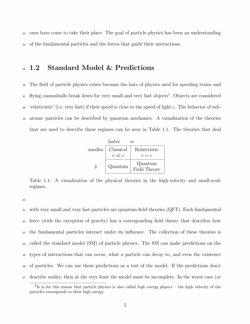
atomic particles can be described by quantum mechanics. A visualization of the theories59

that are used to describe these regimes can be seen in Table 1.1. The theories that deal

faster ⇒smaller Classical Relativistic

v ≪ c v ∼ c

⇓ QuantumQuantum

Field Theory

Table 1.1: A visualization of the physical theories in the high-velocity and small-scaleregimes.

60

with very small and very fast particles are quantum field theories (QFT). Each fundamental61

force (with the exception of gravity) has a corresponding field theory that describes how62

the fundamental particles interact under its influence. The collection of these theories is63

called the standard model (SM) of particle physics. The SM can make predictions on the64

types of interactions that can occur, what a particle can decay to, and even the existence65

of particles. We can use these predictions as a test of the model. If the predictions don’t66

describe reality, then at the very least the model must be incomplete. In the worst case (or67

1It is for this reason that particle physics is also called high energy physics – the high velocity of theparticles corresponds to their high energy.

5

the most interesting case, depending on your point of view) the model will have to be rebuilt.68

New predictions will either point to the model being correct or another reevaluation of the69

model. This cycle of testing and reevaluation is the scientific method. Observations made70

lead to a hypothesis about how the world works which in turn leads to predictions based on71

the hypothesis. These predictions are either confirmed and the hypothesis is strengthened72

or invalidated and the hypothesis discarded. Particle physics is simply the scientific method73

at work with the SM as its testable hypothesis.74

1.3 Notes on Notation75

It is prudent here to summarize a few notational quirks present in particle physics. This76

section is divided into information on coordinate systems, the Einstein summation conven-77

tion, and natural units. This section also has several useful figures describing the coordinate78

system that we use in particle physics that may be useful to refer to in the following chapters.79

1.3.1 Coordinate Systems80

Because of the physical design of particle physics experiments, the coordinate system we81

use when describing various aspects of the experimental side of the field is not the carte-82

sian coordinate system. Colliding particles naturally leads to a coordinate system where83

the incoming particles’ trajectories are aligned along the axis of a cylinder. Because the84

energies of the colliding particles are high, the particles that are produced at the collision85

point preferentially have trajectories that are at a small angle relative to the axis. It is for86

this reason that particle detectors are cylindrical in design. However, because the particles87

produced originate from a collision point, it is convenient to define trajectories by the angle88

6

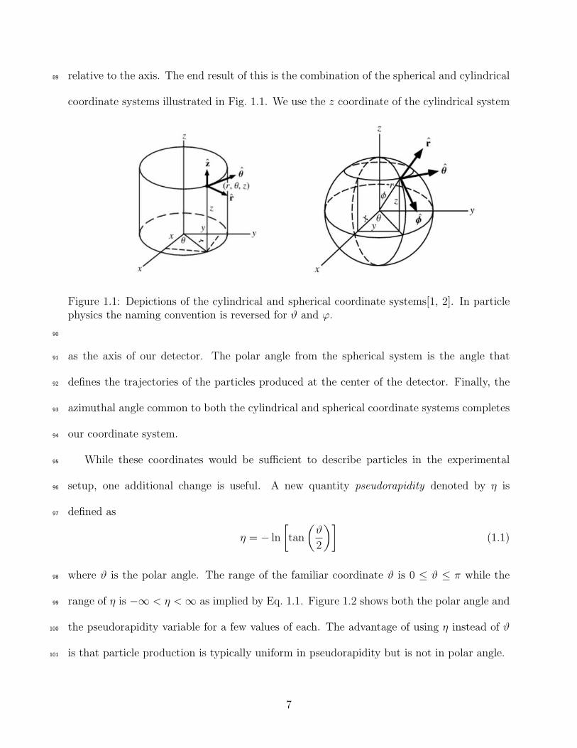
relative to the axis. The end result of this is the combination of the spherical and cylindrical89

coordinate systems illustrated in Fig. 1.1. We use the z coordinate of the cylindrical system

Figure 1.1: Depictions of the cylindrical and spherical coordinate systems[1, 2]. In particlephysics the naming convention is reversed for ϑ and ϕ.

90

as the axis of our detector. The polar angle from the spherical system is the angle that91

defines the trajectories of the particles produced at the center of the detector. Finally, the92

azimuthal angle common to both the cylindrical and spherical coordinate systems completes93

our coordinate system.94

While these coordinates would be sufficient to describe particles in the experimental95

setup, one additional change is useful. A new quantity pseudorapidity denoted by η is96

defined as97

η = − ln

[

tan

(ϑ

2

)]

(1.1)

where ϑ is the polar angle. The range of the familiar coordinate ϑ is 0 ≤ ϑ ≤ π while the98

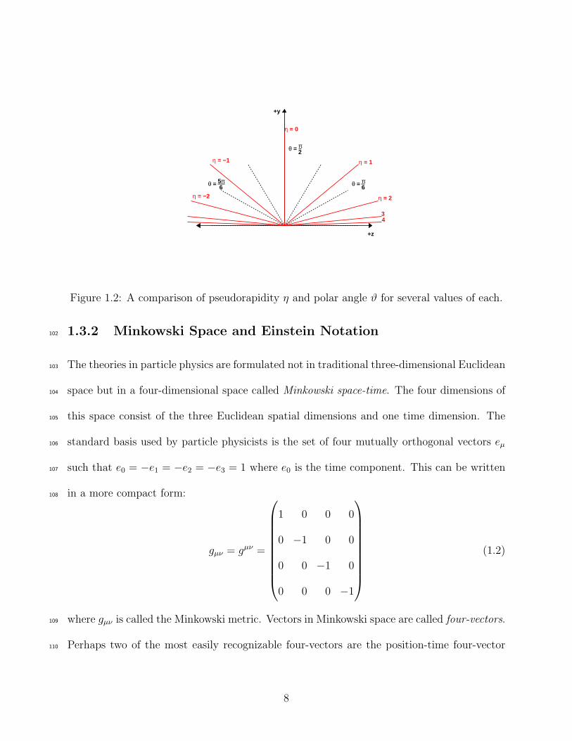
range of η is −∞ < η < ∞ as implied by Eq. 1.1. Figure 1.2 shows both the polar angle and99

the pseudorapidity variable for a few values of each. The advantage of using η instead of ϑ100

is that particle production is typically uniform in pseudorapidity but is not in polar angle.101

7

6π = θ

2π = θ

6π5 = θ

= 0η

= 1η

= 2η

34

= −2η

= −1η

+z

+y

Figure 1.2: A comparison of pseudorapidity η and polar angle ϑ for several values of each.

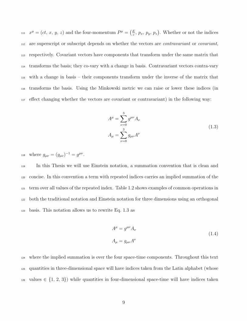
1.3.2 Minkowski Space and Einstein Notation102

The theories in particle physics are formulated not in traditional three-dimensional Euclidean103

space but in a four-dimensional space called Minkowski space-time. The four dimensions of104

this space consist of the three Euclidean spatial dimensions and one time dimension. The105

standard basis used by particle physicists is the set of four mutually orthogonal vectors eµ106

such that e0 = −e1 = −e2 = −e3 = 1 where e0 is the time component. This can be written107

in a more compact form:108

gµν = gµν =

1 0 0 0

0 −1 0 0

0 0 −1 0

0 0 0 −1

(1.2)

where gµν is called the Minkowski metric. Vectors in Minkowski space are called four-vectors.109

Perhaps two of the most easily recognizable four-vectors are the position-time four-vector110

8

xµ = (ct, x, y, z) and the four-momentum P µ =(

Ec, px, py, pz

). Whether or not the indices111

are superscript or subscript depends on whether the vectors are contravariant or covariant,112

respectively. Covariant vectors have components that transform under the same matrix that113

transforms the basis; they co-vary with a change in basis. Contravariant vectors contra-vary114

with a change in basis – their components transform under the inverse of the matrix that115

transforms the basis. Using the Minkowski metric we can raise or lower these indices (in116

effect changing whether the vectors are covariant or contravariant) in the following way:117

Aµ =3∑

ν=0

gµνAν

Aµ =3∑

ν=0

gµνAν

(1.3)

where gµν = (gµν)−1 = gµν .118

In this Thesis we will use Einstein notation, a summation convention that is clean and119

concise. In this convention a term with repeated indices carries an implied summation of the120

term over all values of the repeated index. Table 1.2 shows examples of common operations in121

both the traditional notation and Einstein notation for three dimensions using an orthogonal122

basis. This notation allows us to rewrite Eq. 1.3 as123

Aµ = gµνAν

Aµ = gµνAν

(1.4)

where the implied summation is over the four space-time components. Throughout this text124

quantities in three-dimensional space will have indices taken from the Latin alphabet (whose125

values ∈ 1, 2, 3) while quantities in four-dimensional space-time will have indices taken126

9

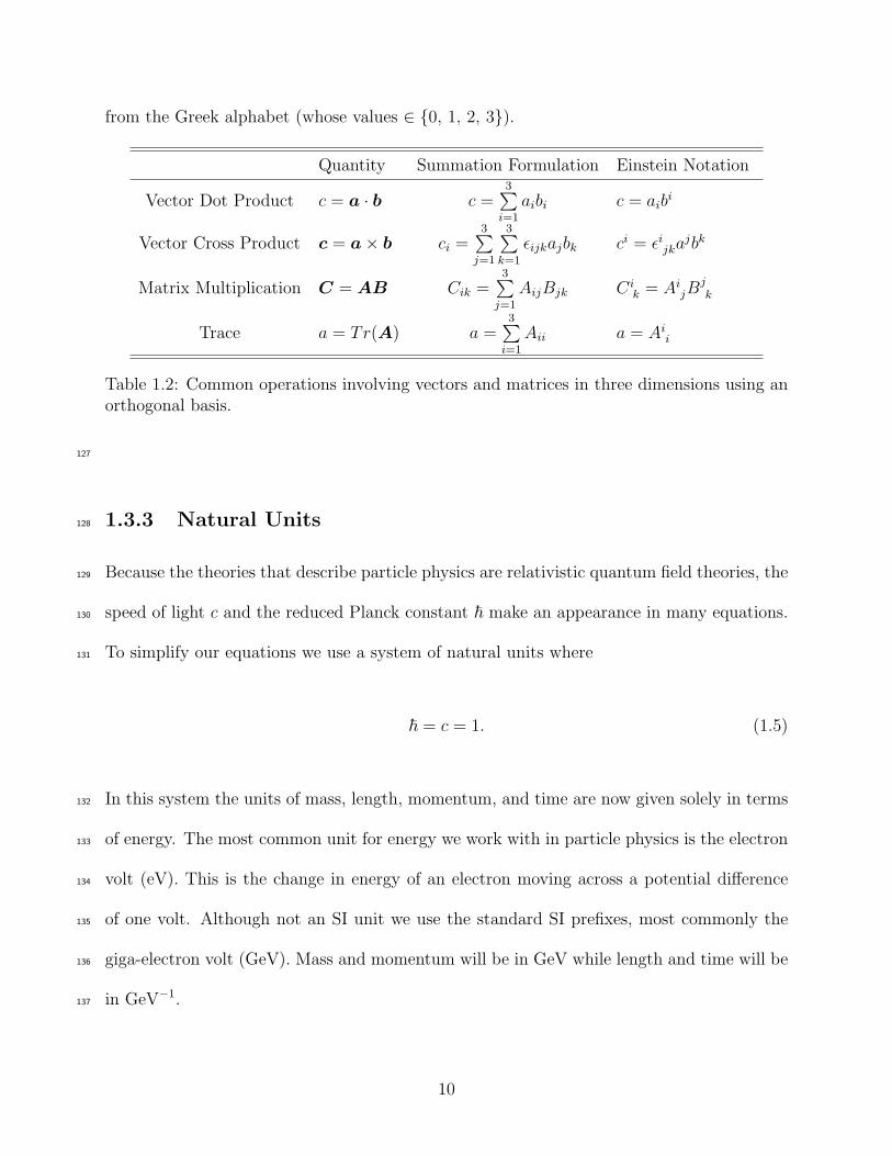
from the Greek alphabet (whose values ∈ 0, 1, 2, 3).

Quantity Summation Formulation Einstein Notation

Vector Dot Product c = a · b c =3∑

i=1

aibi c = aibi

Vector Cross Product c = a × b ci =3∑

j=1

3∑

k=1

ǫijkajbk ci = ǫijka

jbk

Matrix Multiplication C = AB Cik =3∑

j=1

AijBjk Cik = Ai

jBjk

Trace a = Tr(A) a =3∑

i=1

Aii a = Aii

Table 1.2: Common operations involving vectors and matrices in three dimensions using anorthogonal basis.

127

1.3.3 Natural Units128

Because the theories that describe particle physics are relativistic quantum field theories, the129

speed of light c and the reduced Planck constant ~ make an appearance in many equations.130

To simplify our equations we use a system of natural units where131

~ = c = 1. (1.5)

In this system the units of mass, length, momentum, and time are now given solely in terms132

of energy. The most common unit for energy we work with in particle physics is the electron133

volt (eV). This is the change in energy of an electron moving across a potential difference134

of one volt. Although not an SI unit we use the standard SI prefixes, most commonly the135

giga-electron volt (GeV). Mass and momentum will be in GeV while length and time will be136

in GeV−1.137

10

1.4 Tools138

To study elementary particles we need to be able to produce them, record their interactions,139

and then interpret the results. This section will be dedicated to the basics of particle produc-140

tion and detection. It will be built upon in later chapters with descriptions of the machinery141

specific to this Dissertation.142

1.4.1 Particle Acceleration143

To produce interesting and possibly never-before-seen particles we collide matter at high144

energy. The first step in setting up these collisions is the acceleration of particles to velocities145

approaching the speed of light. Current technologies using accelerating fields necessitate the146

use of electrically-charged particles. There are several accelerating schemes but all are based147

on the Lorentz force:148

F = q (E + v × B) (1.6)

where q is the charge of the particle, v is its velocity, and E and B are the electric and149

magnetic fields, respectively. Because the force due to the magnetic field is perpendicular150

to the particle’s velocity it cannot be used to accelerate the particle2. This means that all151

particle acceleration is done using electric fields.152

1.4.1.1 Electrostatic Accelerators153

The simplest type of accelerator uses a static electric field to impart energy to a stream154

of charged particles. This static electric field is produced by generating a constant voltage155

2Technically the magnetic field cannot be used to accelerate a particle in the direction of its velocity–itcan be used to accelerate a particle perpendicular to its direction, a detail that will be discussed later in thesection.

11

difference, similar to the field between capacitor plates. For a free test charge q moving in a156

uniform electric field the energy gained by the test charge is equal to the work done157

W = −q (Vf − Vi) (1.7)

where Vf and Vi are the final and initial voltage respectively. Negative test charges will158

accelerate in the direction opposite the electric field and positive test charges will accelerate159

in the direction of the electric field. To increase the energy gained by the particles you160

can increase their charge or you can increase the voltage difference they accelerate through.161

Depending on the particle species it is possible to add or remove electrons to increase the162

absolute value of the charge. Typically there is a limit to the amount of charge you can163

accumulate so we look to increasing the voltage difference. The high voltages required by164

particle physics experiments are obtained by specialized voltage generators. While there are165

several schemes for generating these high voltages we will discuss the one that is used to166

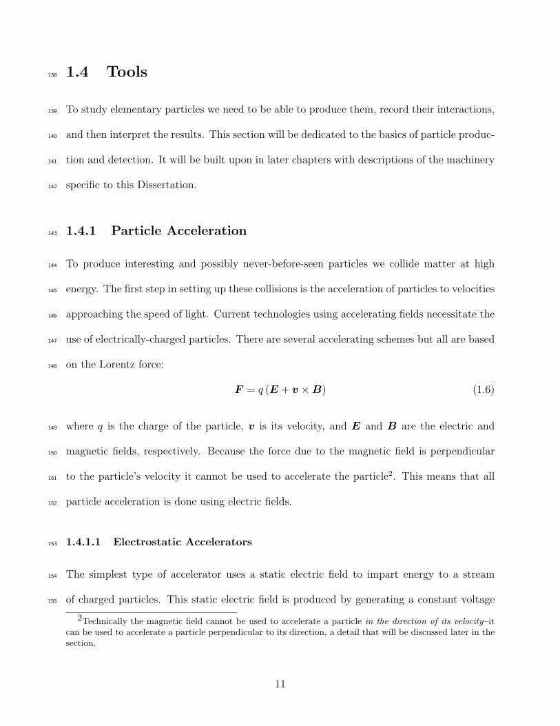
accelerate particles at Fermilab: the Cockcroft-Walton generator.167

The Cockcroft-Walton generator is a voltage multiplier consisting of two stacks of capac-168

itors linked by diodes as shown in Fig. 1.3 and is sometimes referred to as the Cockcroft-169

Walton ladder. The capacitors on the left hold a charge and couple to the alternating current170

(AC) voltage source at the bottom of the stack while the capacitors on the left are DC; the171

charge on them is constant. During the negative half-cycle the capacitors on the left are172

charged. The capacitors on the right are charged during the positive half-cycle. Figure 1.3173

shows only two stages of a Cockcroft-Walton ladder, more can be added on to increase the174

output voltage. For a Cockcroft-Walton ladder with n stages the final output voltage is175

2nV0.176

12

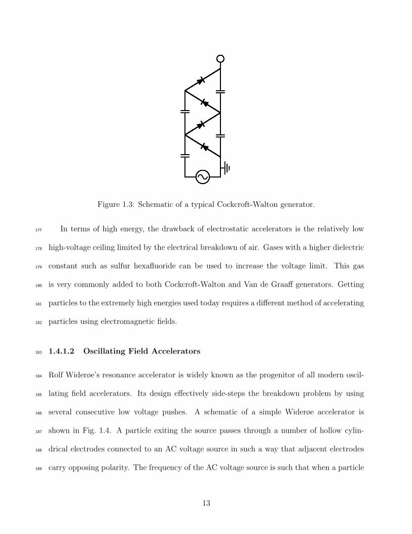
Figure 1.3: Schematic of a typical Cockcroft-Walton generator.

In terms of high energy, the drawback of electrostatic accelerators is the relatively low177

high-voltage ceiling limited by the electrical breakdown of air. Gases with a higher dielectric178

constant such as sulfur hexafluoride can be used to increase the voltage limit. This gas179

is very commonly added to both Cockcroft-Walton and Van de Graaff generators. Getting180

particles to the extremely high energies used today requires a different method of accelerating181

particles using electromagnetic fields.182

1.4.1.2 Oscillating Field Accelerators183

Rolf Widerøe’s resonance accelerator is widely known as the progenitor of all modern oscil-184

lating field accelerators. Its design effectively side-steps the breakdown problem by using185

several consecutive low voltage pushes. A schematic of a simple Widerøe accelerator is186

shown in Fig. 1.4. A particle exiting the source passes through a number of hollow cylin-187

drical electrodes connected to an AC voltage source in such a way that adjacent electrodes188

carry opposing polarity. The frequency of the AC voltage source is such that when a particle189

13

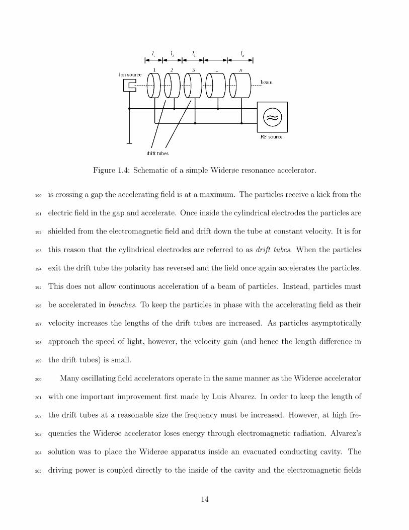
Figure 1.4: Schematic of a simple Widerøe resonance accelerator.

is crossing a gap the accelerating field is at a maximum. The particles receive a kick from the190

electric field in the gap and accelerate. Once inside the cylindrical electrodes the particles are191

shielded from the electromagnetic field and drift down the tube at constant velocity. It is for192

this reason that the cylindrical electrodes are referred to as drift tubes. When the particles193

exit the drift tube the polarity has reversed and the field once again accelerates the particles.194

This does not allow continuous acceleration of a beam of particles. Instead, particles must195

be accelerated in bunches. To keep the particles in phase with the accelerating field as their196

velocity increases the lengths of the drift tubes are increased. As particles asymptotically197

approach the speed of light, however, the velocity gain (and hence the length difference in198

the drift tubes) is small.199

Many oscillating field accelerators operate in the same manner as the Widerøe accelerator200

with one important improvement first made by Luis Alvarez. In order to keep the length of201

the drift tubes at a reasonable size the frequency must be increased. However, at high fre-202

quencies the Widerøe accelerator loses energy through electromagnetic radiation. Alvarez’s203

solution was to place the Widerøe apparatus inside an evacuated conducting cavity. The204

driving power is coupled directly to the inside of the cavity and the electromagnetic fields205

14

are contained inside the conductor. Furthermore, if the resonance frequency of the cavity is206

equal to that of the acceleration frequency the energy transfer is the most efficient. Varia-207

tions on this design lead to many different types of cavities that differ in size, shape, and208

conducting material. Examples of different cavities that operate in the microwave frequency209

range are shown in Fig. 1.5.

Figure 1.5: Examples of cavity shapes that operate in the microwave frequency range. AnAlvarez drift tube cavity and a superconducting cavity made to operate at very low temper-ature.

210

A device which has an advantage over the linear accelerators is the synchrotron. Accel-211

eration is done at one or more sites along a ring and the particle can make many passes212

through the accelerating region(s), gaining energy with every turn. The particles are steered213

using magnets located around the ring. The particles’ orbit has a fixed radius made possible214

by increasing the field strength of the magnets as the particles accelerate. With the devel-215

opment of strong focusing, the concept that alternating focusing and defocusing magnets216

will have a net focusing effect on the beam, we can separate the three functions of the syn-217

chrotron: acceleration, steering, and focusing. The acceleration is typically done in straight218

sections with microwave frequency cavities. The steering is handled with magnetic dipoles219

and the focusing is done with quadrupole and higher multipole magnets. Most accelerators220

that operate on the higher end of the energy spectrum are synchrotrons.221

15

1.4.2 Particle Production222

Relativistic kinematics allows for the production of new matter through the conservation223

of energy and momentum. Colliding particles at high energy and examining the particles224

that are produced as a result is the primary way particle physicists investigate fundamental225

particles and their interactions.226

1.4.2.1 Fixed Target227

One way to collide matter is to use particles to strike a target material. This was the228

mode of operation for many years in the field. The Bevatron (named for its ability to229

impart billions of electron-volts of energy) at Lawrence Berkeley National Lab (LBNL) was230

a machine that accelerated protons into a fixed target. The first antiproton was discovered231

using the Bevatron at LBNL. As an example of relativistic kinematics and the creation of a232

particle we can calculate the minimum energy required to produce a proton-antiproton pair.233

The reaction can be written as follows:234

p + p → p + p + p + p. (1.8)

Having just enough energy to create a proton-antiproton pair would mean there would be235

no extra energy left over for the kinetic energy of the products. It may be hard to formulate236

conditions for this in the frame of reference of the lab but it is relatively easy in the center237

of momentum (CoM) frame, where the total momentum of the system is zero. In this frame238

after the collision all of the products would be at rest. To solve this problem we can use239

the Lorentz invariance of the dot product of two four-vectors, vectors in four dimensional240

space-time. This means that the dot product of two four-vectors is the same in any frame of241

16

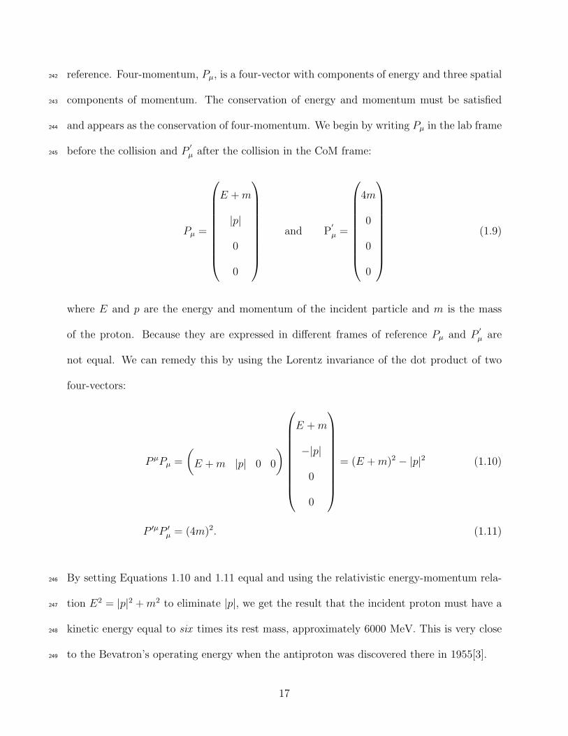
reference. Four-momentum, Pµ, is a four-vector with components of energy and three spatial242

components of momentum. The conservation of energy and momentum must be satisfied243

and appears as the conservation of four-momentum. We begin by writing Pµ in the lab frame244

before the collision and P′

µ after the collision in the CoM frame:245

Pµ =

E + m

|p|

0

0

and P′

µ =

4m

0

0

0

(1.9)

where E and p are the energy and momentum of the incident particle and m is the mass

of the proton. Because they are expressed in different frames of reference Pµ and P′

µ are

not equal. We can remedy this by using the Lorentz invariance of the dot product of two

four-vectors:

P µPµ =

(

E + m |p| 0 0

)

E + m

−|p|

0

0

= (E + m)2 − |p|2 (1.10)

P ′µP ′µ = (4m)2. (1.11)

By setting Equations 1.10 and 1.11 equal and using the relativistic energy-momentum rela-246

tion E2 = |p|2 + m2 to eliminate |p|, we get the result that the incident proton must have a247

kinetic energy equal to six times its rest mass, approximately 6000 MeV. This is very close248

to the Bevatron’s operating energy when the antiproton was discovered there in 1955[3].249

17

This exercise illustrates a major disadvantage of fixed target experiments; much of the250

initial kinetic energy is unavailable for creating new mass. The rest energy of six protons251

is needed to create two. In a sense this energy is ‘wasted’ in the kinetic energy of the final252

products. What if the center of momentum frame was the lab frame? It would then be253

possible to create particles at rest in the lab frame without wasting any energy! While fixed254

target experiments certainly still have their use, if you want the most energy available for255

particle creation you better build a collider.256

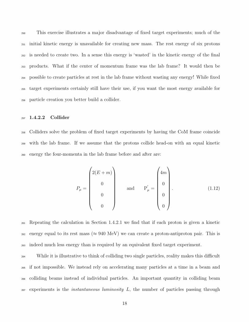
1.4.2.2 Collider257

Colliders solve the problem of fixed target experiments by having the CoM frame coincide258

with the lab frame. If we assume that the protons collide head-on with an equal kinetic259

energy the four-momenta in the lab frame before and after are:260

Pµ =

2(E + m)

0

0

0

and P′

µ =

4m

0

0

0

. (1.12)

Repeating the calculation in Section 1.4.2.1 we find that if each proton is given a kinetic261

energy equal to its rest mass (≈ 940 MeV) we can create a proton-antiproton pair. This is262

indeed much less energy than is required by an equivalent fixed target experiment.263

While it is illustrative to think of colliding two single particles, reality makes this difficult264

if not impossible. We instead rely on accelerating many particles at a time in a beam and265

colliding beams instead of individual particles. An important quantity in colliding beam266

experiments is the instantaneous luminosity L, the number of particles passing through267

18

a plane per unit time per unit area. The higher the instantaneous luminosity, the more268

chances there are for interactions to occur. The luminosity of a particular beam of particles269

is dependent on the physical aspects of the beam, e.g. its size, particle composition, and270

number of particles. Related to luminosity is the concept of a cross section, usually denoted271

by σ, with units of area. The term comes from scattering experiments where particles are272

impinged on a hard sphere. A scattering event will occur if the incident particle is within a273

circular area, the hard sphere’s cross section. Collisions in particle physics are not as simple274

as a collision with a hard sphere, but the term has stuck. Interaction boundaries are fuzzy so275

direct contact is not necessary for an interaction to occur, unlike the hard sphere scattering.276

Additionally, there are a variety of outcomes each with their own probability due to the277

quantum mechanical nature of the interaction. For these reasons, the cross section is not a278

physical description of the size of a particle, but rather an effective cross section of a clearly-279

defined process. A process with a small cross section is a rare event; the probability for it to280

occur is small. Knowing the instantaneous luminosity and a process you are interested in, it281

is possible to calculate how many of those events you can expect per unit time:282

dN

dt= σL (1.13)

where N is the number of events. Integrating both sides of Eq. 1.13 tells us that we can expect283

N events equal to the cross section multiplied by the integrated luminosity, Lint =∫

Ldt.284

One important thing to note is that the cross section for a process can be measured at285

any colliding experiment provided you can measure the luminosity and count the number of286

events.287

19

1.4.2.3 Colliding Particles288

There are many things to consider when deciding what type of particles to collide. Maybe289

the most important of these is choosing a relatively long-lived and charged particle. It290

is important to use long-lived particles that will not decay before they have a chance to291

collide. This is especially important in cyclic colliders where the beams may be in rotation292

for hours. Having a charged particle is necessary because accelerating the particles is done293

using electromagnetic fields or magnetic fields. Protons and electrons are both charged and294

very stable particles that are good candidates for colliders.295

Another consideration is whether the particle is point-like or composite. Colliding point-296

like particles like electrons is a much cleaner process than colliding protons because there297

are fewer particles in the final state. Protons have three valence quarks and typically only298

one quark is involved in a collision, the rest recombine to form additional particles. These299

additional particles not involved in the main interaction nonetheless leave signatures in the300

final state and are detected with those produced in the main interaction. Weeding out these301

additional particles is difficult and the precision of the measurement suffers. Additionally,302

it is difficult to accurately calculate the energy of the collision because the total energy of303

the particle is divided by the constituents. However, this curse is also a gift; there are more304

types of interactions possible with composite particles. If the goal is precision measurements305

then electrons are the way to go. If on the other hand the goal is discovery of new physics306

then protons are the particle of choice.307

So far we’ve assumed that both particles in the collision are identical particles. Another308

possibility is the use of antiparticles: particles with the same mass but opposite charge.309

In some ways this can simplify the design of the particle accelerator. The particles and310

20

antiparticles can share the same beam pipe and the same electromagnetic fields will accelerate311

them in opposite directions. Having identical particles as the colliding particles will require312

a more complicated accelerator complex. At relatively low energies there is an additional313

benefit to using protons and antiprotons due to the energy carried by the constituent quarks.314

At collision energies up to ∼ 3 TeV, most of the energy is carried by the three valence quarks315

with minimal energy carried by the sea quarks and gluons. It is more likely then to get an316

annihilation event by colliding a proton with an antiproton. At higher energies the sea quarks317

and gluons get a higher percentage of the energy and the benefit of using antiparticles is318

reduced. This is fortunate in a way because antiparticles are very hard to produce and store.319

Requiring a charged particle does have a downside for cyclic colliders: synchrotron radi-320

ation. This is a source of energy loss that is proportional to the charge and energy of the321

particle and inversely proportional to the particle mass and radius of the curve. Colliding322

very light, charged particles at very high energy means a very large accelerator. Taking into323

account all these factors to minimize the energy loss is a balancing act.324

1.4.3 Particle Detection325

To learn about particles and their interactions we must have a way to observe them. Tra-326

ditional methods of observation are not feasible and we must rely on their interactions with327

matter to learn about them. Like particle acceleration, particle detection relies heavily on328

charged particle interactions. The next section briefly overviews high energy particle interac-329

tions with matter focusing on electromagnetic interactions and introduces particle showers.330

Section 1.4.3.2 gives an overview of the basic structure of a particle detector.331

21

1.4.3.1 Matter Interactions332

Matter Interactions via the Electromagnetic Force333

All energetic charged particles interact with matter via the electromagnetic force, which334

is mediated by photons. These interactions result in the loss of kinetic energy. These335

interactions can either be with orbital atomic electrons or with atomic nuclei. An interaction336

with an orbital electron can result in excitation or ionization. Excitation occurs when the337

orbital electron gains energy from the passing charged particle and is promoted to a higher338

energy orbital. Following excitation, the orbital electron relaxes back to a lower energy orbit339

and emits a photon in the process. When the energy gained from the passing charged particle340

exceeds the binding energy of that electron, ionization occurs and the electron becomes341

unbound. In an interaction with an atomic nucleus the charged particle may radiate a photon342

as it decelerates, referred to as bremsstrahlung3. The characteristic length associated with343

this type of process is the radiation length X0, both the mean distance through which a344

high energy electron loses all but 1/e of its energy and 7/9 of the mean free path for a high345

energy photon. A charged particle can also scatter off of a nucleus, losing almost no energy346

in the process, and be deflected. This type of scattering is collectively referred to as coulomb347

scattering. The precise mechanism by which particles lose energy and the amount of energy348

lost depends on the mass of the particle, its momentum, and the material. For our purposes,349

we divide our discussion between heavy4 charged particles, electrons, and photons.350

Heavy charged particles interact electromagnetically through ionization and excitation.351

The mean energy loss rate for heavy charged particles can be approximated by the Bethe352

formula which depends on the material, the velocity of the incident particle (β = v/c), and353

3In German, literally “braking radiation”.4‘Heavy’ particles here refer to those more massive than the electron.

22

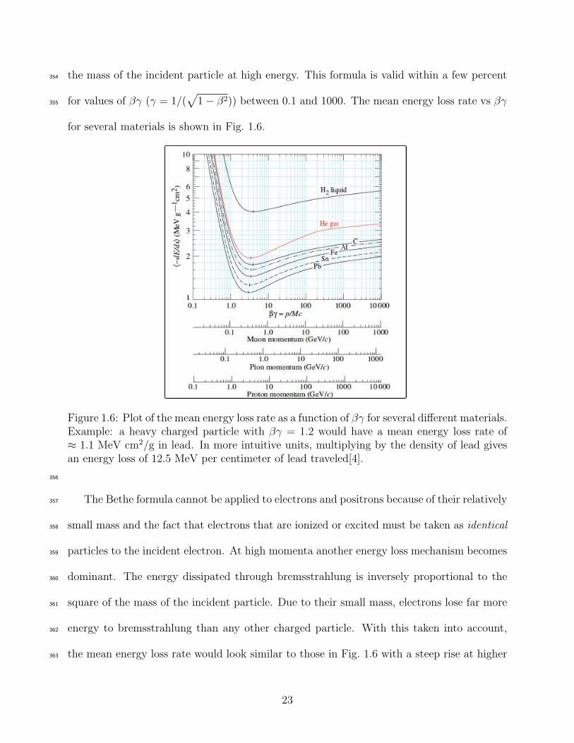
the mass of the incident particle at high energy. This formula is valid within a few percent354

for values of βγ (γ = 1/(√

1 − β2)) between 0.1 and 1000. The mean energy loss rate vs βγ355

for several materials is shown in Fig. 1.6.

Figure 1.6: Plot of the mean energy loss rate as a function of βγ for several different materials.Example: a heavy charged particle with βγ = 1.2 would have a mean energy loss rate of≈ 1.1 MeV cm2/g in lead. In more intuitive units, multiplying by the density of lead givesan energy loss of 12.5 MeV per centimeter of lead traveled[4].

356

The Bethe formula cannot be applied to electrons and positrons because of their relatively357

small mass and the fact that electrons that are ionized or excited must be taken as identical358

particles to the incident electron. At high momenta another energy loss mechanism becomes359

dominant. The energy dissipated through bremsstrahlung is inversely proportional to the360

square of the mass of the incident particle. Due to their small mass, electrons lose far more361

energy to bremsstrahlung than any other charged particle. With this taken into account,362

the mean energy loss rate would look similar to those in Fig. 1.6 with a steep rise at higher363

23

βγ to account for bremsstrahlung and other radiative losses.364

Although the photon does not carry a charge, it can interact electromagnetically as the365

mediator of the electromagnetic force. A photon can be absorbed by an orbital electron366

and either be re-emitted or, if the energy exceeds the binding energy, free the electron from367

its bound state. In the presence of the electromagnetic field of an electron or a nucleus a368

photon can convert into an electron-positron pair provided it has an energy greater than369

1.02 MeV, twice the mass of an electron. At high energy photons primarily lose energy via370

pair production in the field of a nucleus and to a lesser extent in the field of an orbital371

electron.372

Matter Interactions via the Strong Force373

As far as we can tell, nature has determined that quarks and gluons must be confined in374

hadrons as detailed by the theory governing the strong force. The property of confinement375

will be discussed in further detail in Chapter 2 but for our purposes here it is sufficient to376

grant its existence. The result of this property is that any gluons or quarks produced in the377

collision immediately form hadrons or ‘hadronize’ by combining with quark-antiquark pairs378

from the vacuum. Hadrons, whether charged or neutral, can interact with matter via the379

strong force. The characteristic distance in this type of interaction is the nuclear interaction380

length λA and is the mean distance a hadronic particle travels before interacting with a381

nuclei in the material.382

Particle Showers383

When enough material is present and the particle’s energy is high enough a particle384

shower can form. Incident particles, whether charged or neutral, interact with matter and385

24

produce secondary particles. If the energy imparted to the secondaries is large, they can also386

interact and produce additional particles. This continues until the resulting particles do not387

have enough energy to produce new particles. These particles continue to lose energy via388

ionization and excitation until they are captured or absorbed into the material. Two types389

of showers occur in a particle detector: electromagnetic showers and hadronic showers.390

EM showers begin with a high energy photon or electron. An electron, perhaps, interacts391

with a nucleus and emits a photon. This photon then produces an electron-positron pair392

and each emit a photon through bremsstrahlung. The shower continues in this manner until393

the energy has decreased below the point at which pair production or bremsstrahlung is the394

dominant mode of energy loss. The particles continue to lose energy by other methods. The395

characteristic length scale of shower formation is the radiation length X0.396

Hadronic showers begin with a high energy hadron. The hadron interacts with the nuclei397

of the detector material producing more quarks and gluons which immediately hadronize.398

Secondary particles with enough energy continue to interact until their energy is too low399

and they are captured by the detector material. The shower depth scales as the nuclear400

interaction length λA. Because λA is in general larger than the radiation length, hadronic401

showers take longer to form than EM showers. It happens then that electromagnetic showers402

occur within hadronic showers when secondary particles interact electromagnetically.403

Neutrinos404

It is worth noting here that of all the particles, neutrinos are the only ones that don’t405

interact via the electromagnetic or strong force. They only interact via the weak force which406

has a very short interaction range. Neutrinos can therefore pass through large amounts of407

matter without interacting and remain undetected by most multipurpose detectors. Their408

25

existence is inferred from the momentum imbalance or missing transverse energy 6ET in409

particle collisions.410

1.4.3.2 Detectors411

The second piece of equipment necessary for a particle physics experiment is a detector.412

The detector acts as a camera that records information about the collision and the particles413

that were created. Because the design of cyclic accelerators allows for multiple interaction414

points, it is common for there to be multiple detectors at each of these accelerator complexes.415

Detectors are roughly cylindrical in shape and are situated around the collision point. To416

maximize the number of physics studies that can be done most detectors are general purpose417

– they are designed to detect many different types of signatures.418

All detector components make use of electromagnetic interactions, especially ionization419

and excitation, to obtain information on passing particles. Ionization results in a free electron420

and a positive ion generally referred to as a hole. These electron-hole pairs can be collected421

and the charge measured. Photons emitted during excitations can be measured as light in a422

plastic scintillator. Tracking systems for multipurpose detectors are developed to trace the423

path of a particle without disturbing its trajectory by using small amounts of low atomic424

number and low atomic mass material. The particle momentum can be measured for charged425

particles by measuring the curvature of their track in a magnetic field. Calorimeters are used426

to measure the energy of a particle by initiating particle showers with high density materials427

and measuring the total energy deposited by charge collection or scintillation light.428

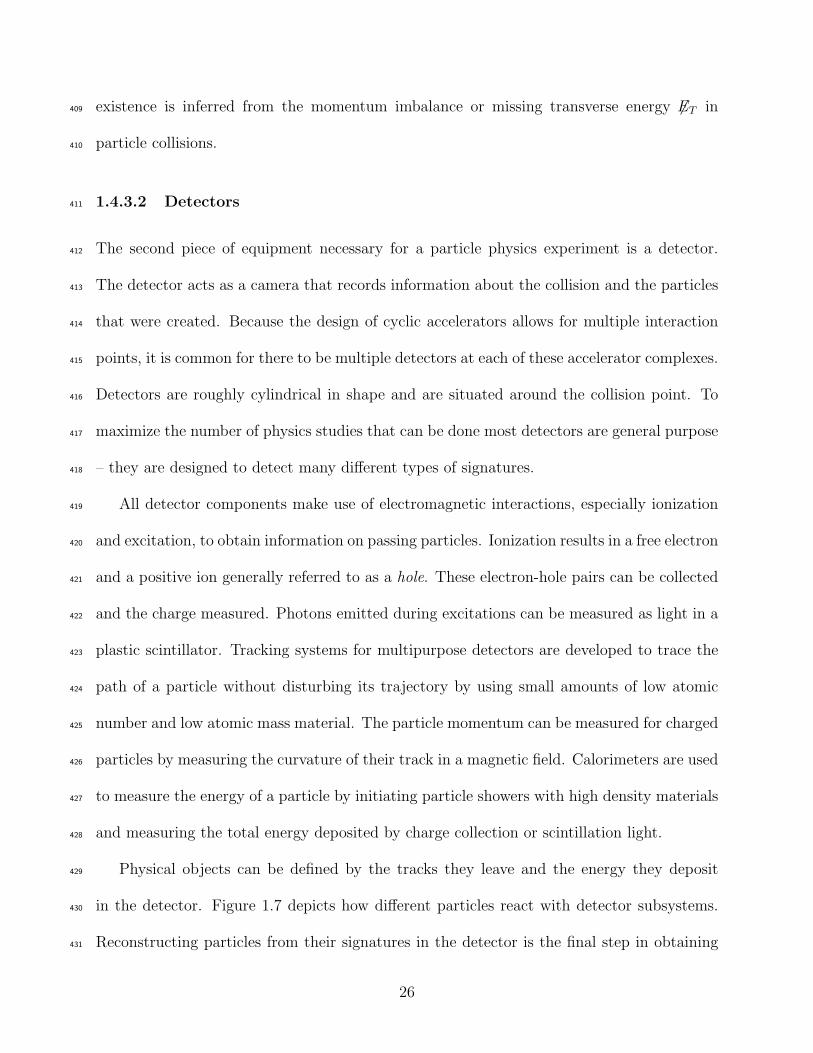
Physical objects can be defined by the tracks they leave and the energy they deposit429

in the detector. Figure 1.7 depicts how different particles react with detector subsystems.430

Reconstructing particles from their signatures in the detector is the final step in obtaining431

26

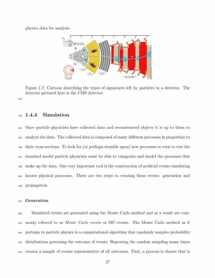
physics data for analysis.

Figure 1.7: Cartoon describing the types of signatures left by particles in a detector. Thedetector pictured here is the CMS detector.

432

1.4.4 Simulation433

Once particle physicists have collected data and reconstructed objects it is up to them to434

analyze the data. The collected data is composed of many different processes in proportion to435

their cross sections. To look for (or perhaps stumble upon) new processes or even to test the436

standard model particle physicists must be able to categorize and model the processes that437

make up the data. One very important tool is the construction of artificial events simulating438

known physical processes. There are two steps to creating these events: generation and439

propagation.440

Generation441

Simulated events are generated using the Monte Carlo method and as a result are com-442

monly referred to as Monte Carlo events or MC events. The Monte Carlo method as it443

pertains to particle physics is a computational algorithm that randomly samples probability444

distributions governing the outcome of events. Repeating the random sampling many times445

creates a sample of events representative of all outcomes. First, a process is chosen that is446

27

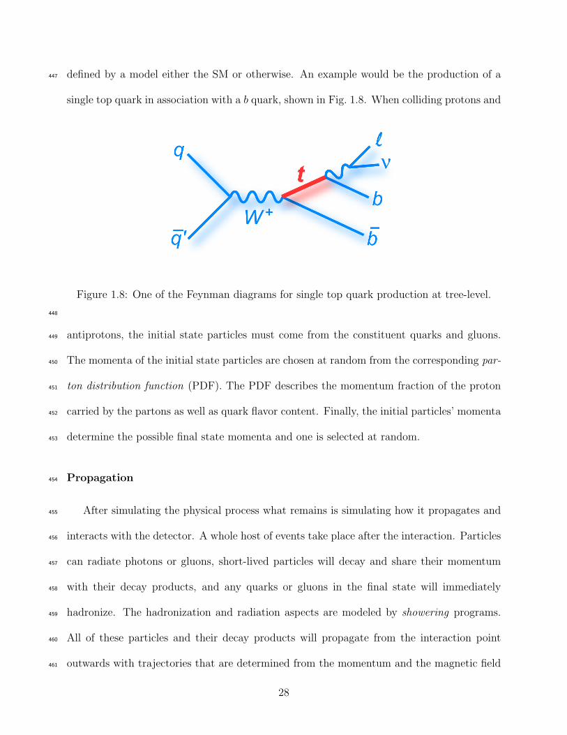
defined by a model either the SM or otherwise. An example would be the production of a447

single top quark in association with a b quark, shown in Fig. 1.8. When colliding protons and

Figure 1.8: One of the Feynman diagrams for single top quark production at tree-level.

448

antiprotons, the initial state particles must come from the constituent quarks and gluons.449

The momenta of the initial state particles are chosen at random from the corresponding par-450

ton distribution function (PDF). The PDF describes the momentum fraction of the proton451

carried by the partons as well as quark flavor content. Finally, the initial particles’ momenta452

determine the possible final state momenta and one is selected at random.453

Propagation454

After simulating the physical process what remains is simulating how it propagates and455

interacts with the detector. A whole host of events take place after the interaction. Particles456

can radiate photons or gluons, short-lived particles will decay and share their momentum457

with their decay products, and any quarks or gluons in the final state will immediately458

hadronize. The hadronization and radiation aspects are modeled by showering programs.459

All of these particles and their decay products will propagate from the interaction point460

outwards with trajectories that are determined from the momentum and the magnetic field461

28

within the detector. The particles that make it to the detector volume, most of which are462

stable, will interact with the detector material as described in Section 1.4.3.1. A model463

of the detector is constructed for this purpose and includes the active material, support464

structures, magnetic fields, detection thresholds and efficiencies, and geometric structure.465

Particles are propagated through the detector model and their interactions are recorded in466

the same format as real data.467

29

Chapter 2468

Theory469

2.1 Introduction470

In studying fundamental particles and their interactions it becomes necessary to move away471

from describing dynamics as systems of particles and towards systems of fields. While there472

are several reasons this becomes apparent perhaps the easiest way to come to terms with473

this is realizing that there is no reason to assume a relativistic process can be described by a474

single particle alone. Einstein’s mass-energy relation E = mc2 allows for the production of475

particle/antiparticle pairs. Other virtual particles, allowed to exist by Heisenberg’s uncer-476

tainty principle ∆E · ∆t ≥ ~

2for very short times, can appear in second order calculations.477

It makes the most sense then to instead describe systems of fields. This chapter will describe478

the field theories of particle physics.479

In nature we know of four fundamental forces:480

strong force responsible for the binding of quarks in hadrons; the residual effects of this481

force bind the protons in a nucleus482

electromagnetic force that governs the interactions between charged particles483

weak force that accounts for processes such as nuclear beta decay and the decay of the484

muon485

gravitational force that results in planetary orbits486

30

During the classical era in particle physics when all matter was perceived as nothing more487

than protons, neutrons and electrons, the two known forces were electromagnetism and488

gravity. This was due to the infinite range of the electromagnetic and gravitational forces.489

The strong and weak forces on the other hand have a very short range so were not recognizable490

until it was possible to examine objects on a very short length scale. We shall see that each491

of these forces (with the possible exception of gravity) is mediated by the exchange of one or492

more particles. These force carriers can be thought of as messengers between two particles493

that tell them how to interact through the force. We will also see that two of these forces are494

actually different aspects of a single force. All of these forces have a relativistic description.495

Three of them have a quantum description; their force carriers are the quanta of the field.496

Gravity presents a bit of a problem. Unlike the other forces, there is no satisfactory quantum497

theory of gravity at present and no force carrier has yet been discovered. For this reason, it498

will not be discussed in the following chapter. Section 2.2 describes the quantum field theories499

that made up the standard model in particle physics. Section 2.1.1 gives an overview of the500

particle types and families in the standard model. An overview of the searches for the Higgs501

boson is given in Section 2.3. A discussion of what physics may exist beyond the standard502

model is given in Section 2.4.503

2.1.1 Particle Zoo504

Before we dive into the description of the standard model theories, it is helpful to give an505

overview of the many types of particles, both composite and fundamental, that exist in the506

SM.507

Fundamental particles can be divided into quarks, leptons, and mediators. Quarks are508

the building blocks of protons, neutrons, and other particles like them. The group of leptons509

31

include the familiar electron and neutrino. The most recognizable mediator is the photon,510

the light quantum. The six quarks and six leptons are divided into three families of two each511

differing only in mass. The first family consists of the up quark (u), the down quark (d), the512

electron (e), and the electron neutrino (νe). This family is all that is needed to make the513

ordinary matter around us: protons, neutrons, nuclei, and atoms. Table 2.1 gives the names514

and symbols for the three families of quarks and leptons.

Quarks Leptons

First Familyup u electron edown d electron neutrino νe

Second Familycharm c muon µstrange s muon neutrino νµ

Third Familytop t tau τbottom b tau neutrino ντ

Table 2.1: A list of the quarks and leptons in each of the three families.

515

One attribute of particles is the intrinsic quantum number spin. Spin does not represent516

any sort of motion with respect to an axis, but is an intrinsic property of a particle. You517

can divide the group of all particles into two categories based on spin: fermions and bosons.518

Fermions have half-integer spin while bosons have integer spin. The difference in spin leads519

to a very strange property. Fermions follow the Pauli exclusion principle: no two identical520

particles can occupy the same state. Bosons do not follow this rule and arbitrarily many521

bosons can occupy the same state. All leptons and quarks are fermions and all force mediators522

are bosons.523

Parity (P ) is another intrinsic quantum number of particles. It refers to how the particle524

wavefunction transforms under a parity operation. In four-dimensional space-time a parity525

32

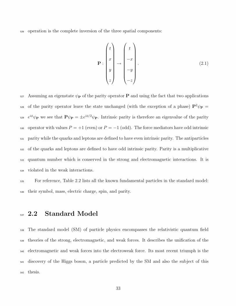
operation is the complete inversion of the three spatial components:526

P :

t

x

y

z

→

t

−x

−y

−z

. (2.1)

Assuming an eigenstate ψP of the parity operator P and using the fact that two applications527

of the parity operator leave the state unchanged (with the exception of a phase) P2ψP =528

eiφψP we see that PψP = ±eiφ/2ψP. Intrinsic parity is therefore an eigenvalue of the parity529

operator with values P = +1 (even) or P = −1 (odd). The force mediators have odd intrinsic530

parity while the quarks and leptons are defined to have even intrinsic parity. The antiparticles531

of the quarks and leptons are defined to have odd intrinsic parity. Parity is a multiplicative532

quantum number which is conserved in the strong and electromagnetic interactions. It is533

violated in the weak interactions.534

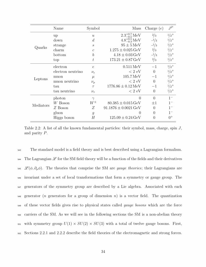
For reference, Table 2.2 lists all the known fundamental particles in the standard model:535

their symbol, mass, electric charge, spin, and parity.536

2.2 Standard Model537

The standard model (SM) of particle physics encompasses the relativistic quantum field538

theories of the strong, electromagnetic, and weak forces. It describes the unification of the539

electromagnetic and weak forces into the electroweak force. Its most recent triumph is the540

discovery of the Higgs boson, a particle predicted by the SM and also the subject of this541

thesis.542

33

Name Symbol Mass Charge (e) JP

Quarks

up u 2.3+0.7−0.5 MeV 2/3 1/2

+

down d 4.8+0.5−0.3 MeV -1/3 1/2

+

strange s 95 ± 5 MeV -1/3 1/2+

charm c 1.275 ± 0.025 GeV 2/3 1/2+

bottom b 4.18 ± 0.03 GeV -1/3 1/2+

top t 173.21 ± 0.87 GeV 2/3 1/2+

Leptons

electron e 0.511 MeV −1 1/2+

electron neutrino νe < 2 eV 0 1/2+

muon µ 105.7 MeV −1 1/2+

muon neutrino νµ < 2 eV 0 1/2+

tau τ 1776.86 ± 0.12 MeV −1 1/2+

tau neutrino ντ < 2 eV 0 1/2+

Mediators

photon γ 0 0 1−

W Boson W± 80.385 ± 0.015 GeV ±1 1−

Z Boson Z 91.1876 ± 0.0021 GeV 0 1−

gluon g 0 0 1−

Higgs boson H 125.09 ± 0.24 GeV 0 0+

Table 2.2: A list of all the known fundamental particles: their symbol, mass, charge, spin J ,and parity P .

The standard model is a field theory and is best described using a Lagrangian formalism.543

The Lagrangian L for the SM field theory will be a function of the fields and their derivatives544

L (φ, ∂µφ). The theories that comprise the SM are gauge theories ; their Lagrangians are545

invariant under a set of local transformations that form a symmetry or gauge group. The546

generators of the symmetry group are described by a Lie algebra. Associated with each547

generator (n generators for a group of dimension n) is a vector field. The quantization548

of these vector fields gives rise to physical states called gauge bosons which are the force549

carriers of the SM. As we will see in the following sections the SM is a non-abelian theory550

with symmetry group U(1) × SU(2) × SU(3) with a total of twelve gauge bosons. First,551

Sections 2.2.1 and 2.2.2 describe the field theories of the electromagnetic and strong forces.552

34

Section 2.2.3 describes the unification of the electromagnetic and weak forces under the553

Glashow-Weinberg-Salam (GWS) theory of weak interactions. Finally, Section 2.2.4 gives554

an overview of electroweak symmetry breaking and an introduction to the Higgs boson.555

2.2.1 Quantum Electrodynamics556

Quantum electrodynamics (QED) was the first formulation of a theory of particle interactions557

that took into account both quantum mechanics and special relativity. It is a relativistic558

quantum field theory that describes the interactions between electrically charged particles.559

The theory was a tremendous success in explanatory and predictive power and to this day,560

it boasts the highest agreement with experimental data. Because it was the first theory561

of its kind (and, in part, because of its wild success) other quantum field theories, such as562

quantum chromodynamics (QCD), are modeled after it.563

We begin by writing the Lorentz-invariant Dirac Lagrangian for a free electron:564

L Dirac = ψ (iγµ∂µ − m) ψ (2.2)

where ψ is a Dirac spinor with a Lorentz-invariant adjoint ψ = ψ†γ0 and the γµ are the Dirac565

matrices γ0 =

0 1

1 0

and γi =

0 σi

−σi 0

1. We then require our field to be invariant566

under the following transformation:567

ψ(x) → eiαxψ(x). (2.3)

This transformation is a phase rotation through an angle α(x) and it defines the symmetry568

1Here the σi are the Pauli matrices σ1 =

(0 11 0

)

, σ2 =

(0 −i

i 0

)

, and σ3 =

(1 00 −1

)

.

35

group U(1), the unitary group of dimension 1. The second term in Eq. 2.2 is invariant under569

this transformation but the first term is not. It is unclear what the derivative of the complex570

field should be when the field transformation at each point in space is different. We must571

introduce a new derivative that transforms like the field: the covariant derivative. For the572

transformation under U(1) symmetry, the covariant derivative takes the form Dµ = ∂µ+ieAµ573

where e is the electron charge and Aµ is a new vector field. We can identify the new574

vector field with the familiar electromagnetic four-potential. This is the single gauge field575

expected by the Lie algebra of U(1) and the quantum of this field is the photon. To complete576

the QED Lagrangian we must include a kinetic term for the four-potential that is locally577

invariant and does not depend on the field. We introduce the electromagnetic field tensor578

Fµν = ∂µAν − ∂νAµ for this purpose. The full QED Lagrangian can then be written as:579

L QED = ψ(iγµ∂µ − m)ψ︸ ︷︷ ︸

L Dirac

− eψγµAµψ︸ ︷︷ ︸

L int

+ 14(Fµν)

2

︸ ︷︷ ︸

L Maxwell

. (2.4)

The first term of Eq. 2.4 is just the Dirac equation we began with and the middle term580

describes the interaction between the field and the four-potential. Applying the Euler-581

Lagrange equation to the last term yields the inhomogeneous Maxwell equations. The QED582

Lagrangian describes the interactions of all massive spin-1/2 particles with the electromagnetic583

force which includes all the quarks and charged leptons.584

2.2.2 Quantum Chromodynamics585

Quantum chromodynamics (QCD) is the theory that describes strong interactions. Its devel-586

opment began with the conception of the quark model, used to explain the many mesons and587

baryons discovered in the ’50s and ’60s. The early quark model had two problems: quarks588

36

that didn’t appear to obey Fermi-Dirac statistics and particles with a fractional charge could589

not be found. Quarks are fermions; their wavefunctions must be antisymmetric under ex-590

change. This problem with the early quark model can be illustrated by the ∆++ particle, a591

spin-3/2 particle with charge +2. This particle can be explained as a bound state of three up592

quarks with parallel spin – symmetric in flavor and spin. To solve this, it was proposed that593

an additional (hidden) quantum number was carried by quarks and that all baryons were594

antisymmetric in this hidden quantum number. This quantum number is called color and it595

represents an internal SU(3) symmetry.596

Closely related to the second problem with the early quark model is the discovery that597

electron-proton scattering exhibited Bjorken scaling 2; at high enough energies (or a short598

enough timescale) the constituents of the proton behaved as free particles. How is it possible599

then that quarks only weakly interact yet are so tightly bound that they don’t exist freely in600

nature? The answer to this lies in asymptotic freedom, the cornerstone of QCD. Asymptotic601

freedom is a property that causes interactions between particles to become weaker at high602

energies and short timescales and stronger at low energies and long timescales. The Nobel603

Prize in physics for 2004 was awarded to Wilczek, Gross, and Politzer for their 1973 discovery604

of asymptotic freedom in non-abelian3 gauge theories and their relation to strong dynamics[5,605

6].606

Quantum Chromodynamics is a non-abelian gauge theory with local SU(3) color sym-607

metry. In its most compact form the QCD Lagrangian looks almost identical to the QED608

2Properties that exhibit Bjorken scaling are found to be independent of the energy at which the experimentis performed while depending on dimensionless kinematic quantities like a scattering angle. Named for JamesBjorken who found that structure functions of nucleons exhibited this behavior, strongly implying that thenucleons had point-like substructure.

3Unlike the abelian gauge theory QED, the generators of a non-abelian gauge theory do not commute.It is this characteristic that allows non-abelian gauge theories to be asymptotically free.

37

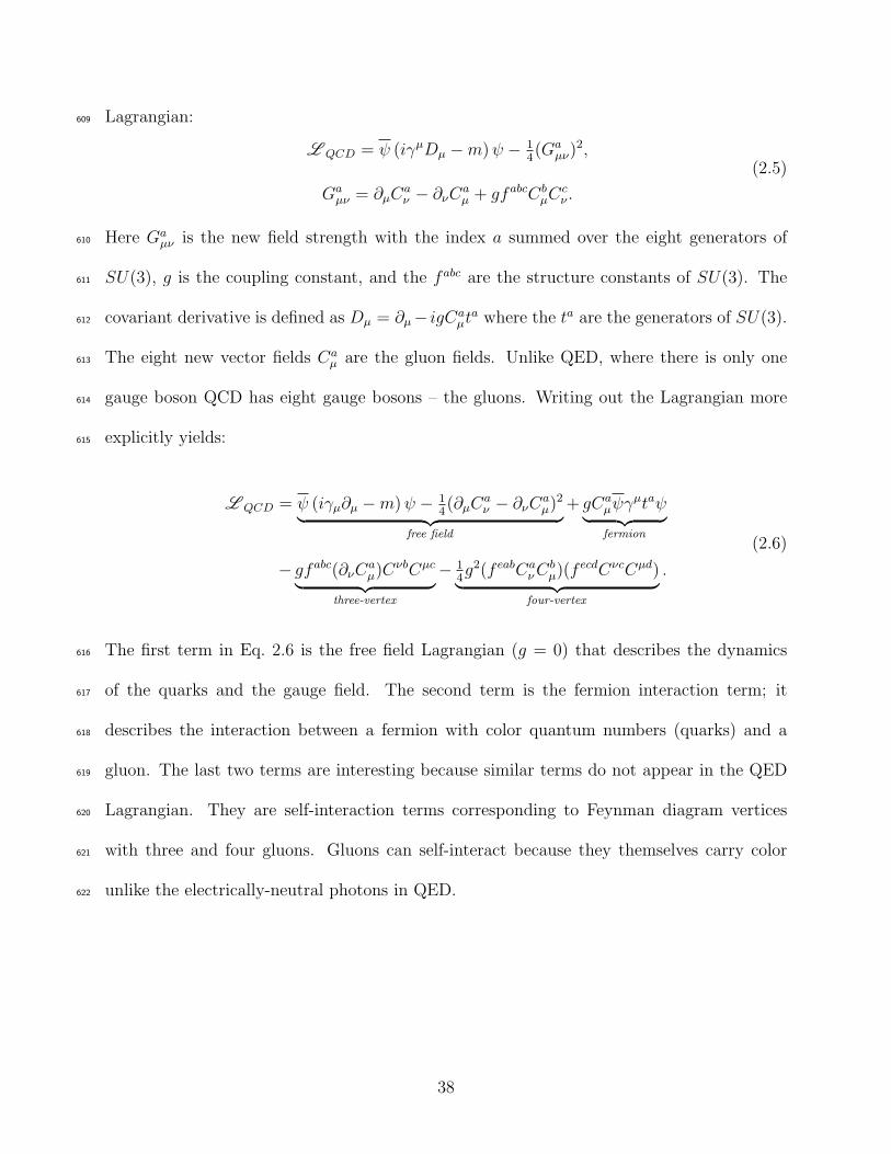
Lagrangian:609

L QCD = ψ (iγµDµ − m) ψ − 14(Ga

µν)2,

Gaµν = ∂µC

aν − ∂νC

aµ + gfabcCb

µCcν .

(2.5)

Here Gaµν is the new field strength with the index a summed over the eight generators of610

SU(3), g is the coupling constant, and the fabc are the structure constants of SU(3). The611

covariant derivative is defined as Dµ = ∂µ− igCaµta where the ta are the generators of SU(3).612

The eight new vector fields Caµ are the gluon fields. Unlike QED, where there is only one613

gauge boson QCD has eight gauge bosons – the gluons. Writing out the Lagrangian more614

explicitly yields:615

L QCD = ψ (iγµ∂µ − m) ψ − 14(∂µC

aν − ∂νC

aµ)2

︸ ︷︷ ︸

free field

+ gCaµψγµtaψ

︸ ︷︷ ︸

fermion

− gfabc(∂νCaµ)CνbCµc

︸ ︷︷ ︸

three-vertex

− 14g2(f eabCa

ν Cbµ)(f ecdCνcCµd)

︸ ︷︷ ︸

four-vertex

.

(2.6)

The first term in Eq. 2.6 is the free field Lagrangian (g = 0) that describes the dynamics616

of the quarks and the gauge field. The second term is the fermion interaction term; it617

describes the interaction between a fermion with color quantum numbers (quarks) and a618

gluon. The last two terms are interesting because similar terms do not appear in the QED619

Lagrangian. They are self-interaction terms corresponding to Feynman diagram vertices620

with three and four gluons. Gluons can self-interact because they themselves carry color621

unlike the electrically-neutral photons in QED.622

38

2.2.3 Glashow-Weinberg-Salam Theory of Weak Interactions623

Formulating a theory of the weak force interactions presents a few problems. First, it has624

been experimentally observed that the W boson only couples to left-handed particles. Worse,625

it appears that right-handed neutrinos do not exist. Second, field theories with unbroken626

symmetries only have massless gauge bosons but the masses of the W and Z bosons are627

certainly not zero – they are quite heavy! As we shall see in Section 2.2.4 the mechanism628

for giving the weak vector bosons mass involves spontaneously breaking the symmetry of629

the electroweak sector. The first problem can be solved in part by assigning right- and630

left-handed fields to different representations of the gauge group.631

These difficulties are a small price to pay for the end result: a theory which gives a632

unified description of the electromagnetic and weak interactions. This means that the elec-633

tromagnetic and weak forces are really different aspects of the same force, the electroweak634

force. Glashow[7], Weinberg[8], and Salam[9] (GWS) introduced the theory which describes635

the weak interactions and also agrees with experiment. For this they won the Nobel Prize636

in physics in 1979.637

We begin as always by requiring a local gauge invariance. For the GWS theory it is a638

SU(2) × U(1) gauge invariance: ψ → eiωiT i

eiβY ψ where the T i are the generators of SU(2)639

with i = 1, 2, 3, β and ωi are arbitrary phases, and Y is the weak hypercharge4 of U(1). For640

a fermion field belonging to the general representation of SU(2) the covariant derivative has641

the form642

Dµ = ∂µ − igW iµT

i − ig′Y Bµ (2.7)

where the W iµ are the vector fields of SU(2) and Bµ is the vector field of U(1). The kinetic643

4Weak hypercharge relates the electric charge Q to the third component of weak isospin T3 by Q = T3+Y .In fact, this equality will become evident in our discussion of electroweak theory.

39

energy terms in the Lagrangian for the gauge fields are644

L kinetic = −14W i

µνWµνi − 1

4BµνB

µν

W iµν = ∂µW

iν − ∂νW

iµ + gǫijkW j

µW kν

Bµν = ∂µBν − ∂νBµ

(2.8)

which are similar to the kinetic terms in QED and QCD. We now incorporate the fact that645

the W bosons only interact with left-handed fermions by assigning the left-handed fermions646

to doublets of SU(2) and right-handed fermions to singlets of SU(2). To reinforce the fact647

that the doublets and singlets belong to different representations of SU(2) we will denote the648

doublets as ψL and the singlets as χR. The singlets of SU(2) only interact with the Bµ field649

leading to the Lagrangian L R = iχRγµ(∂µ − ig′Y Bµ)χR. The doublets interact with both650

fields L L = iψLγµ(∂µ − igW iµT

i − ig′Y Bµ)ψL. The values of the charge Y are determined651

by the species of fermion. The quark fields consist of one left-handed doublet QL = ( ud )L652

and two right-handed singlets uR and dR. Similarly for the leptons, EL = ( νe

e− )L and eR. It653

is tempting to assign the three gauge fields W iµ to the three weak vector bosons W± and654

Z and the Bµ field to the photon but that would imply that the Z boson does not couple655

to right-handed fermions and this is not the case. The role of W iµ and Bµ in producing the656

vector bosons is made clear if we instead write Eq.2.7 in terms of the mass eigenstates of the657

fields. For this we need to break the symmetry of the GWS theory.658

40

2.2.4 Electroweak Symmetry Breaking659

The method of generating gauge boson masses through spontaneous symmetry breaking was660

first5 described independently by Higgs[10]; Brout and Englert[11]; and Guralnik, Hagen,661

and Kibble[12]. In 2013 Higgs and Englert won the Nobel Prize in physics for this work.662

Spontaneous electroweak symmetry breaking (EWKSB) can be incorporated into the GWS663

theory.664

To break the electroweak symmetry spontaneously we introduce a doublet of complex665

scalar fields666

Φ =1√2

φ+

φ0

with φ+ = φ1 + iφ2 and φ0 = φ3 + iφ4

(2.9)

with a self-interaction potential of the form V (Φ) = µ2Φ†Φ + λ(Φ†Φ)2. To preserve the667

symmetry of the electromagnetic sector we assign the scalar field a hypercharge Y of +1/2668

which fixes the electromagnetic charges of the components of Φ. The covariant derivative of669

Φ follows from Eq. 2.7: DµΦ = (∂µ − ig2W i

µσi − ig′

2Bµ)Φ where T i has been expanded as σi

2.670

We can write the Lagrangian as a kinetic term and a potential term671

L = |DµΦ|2 − V (Φ)

= |DµΦ|2︸ ︷︷ ︸

kinetic term

−µ2Φ†Φ − λ(Φ†Φ

)2

︸ ︷︷ ︸

potential terms

.(2.10)

Let’s first look at the potential terms in the Lagrangian. Assuming µ2 < 0 and λ > 0,672

one component of the potential V (Φ) is plotted in the imaginary plane in Fig. 2.1 with673

5Spontaneous symmetry breaking in an abelian gauge theory had already been used to explain the Meiss-ner effect in superconductivity. The application to non-abelian gauge theories and the implications to particlephysics was what was first described by Higgs, et al.

41

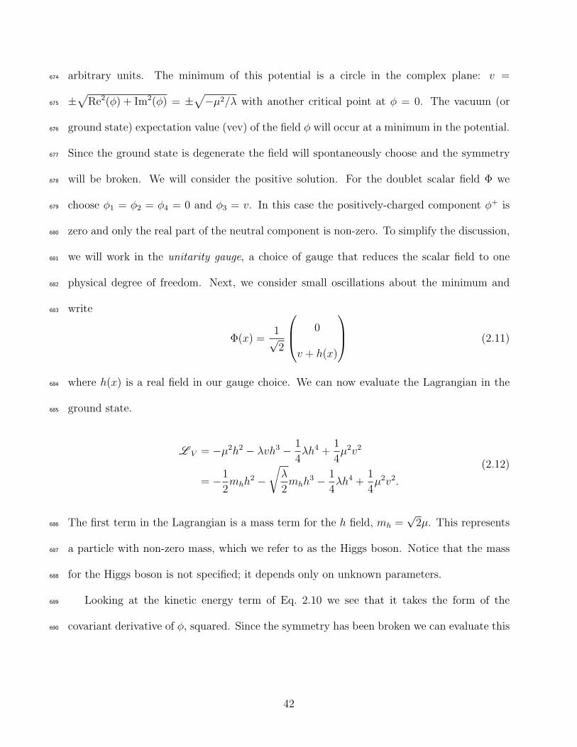
arbitrary units. The minimum of this potential is a circle in the complex plane: v =674

±√

Re2(φ) + Im2(φ) = ±√

−µ2/λ with another critical point at φ = 0. The vacuum (or675

ground state) expectation value (vev) of the field φ will occur at a minimum in the potential.676

Since the ground state is degenerate the field will spontaneously choose and the symmetry677

will be broken. We will consider the positive solution. For the doublet scalar field Φ we678

choose φ1 = φ2 = φ4 = 0 and φ3 = v. In this case the positively-charged component φ+ is679

zero and only the real part of the neutral component is non-zero. To simplify the discussion,680

we will work in the unitarity gauge, a choice of gauge that reduces the scalar field to one681

physical degree of freedom. Next, we consider small oscillations about the minimum and682

write683

Φ(x) =1√2

0

v + h(x)

(2.11)

where h(x) is a real field in our gauge choice. We can now evaluate the Lagrangian in the684

ground state.685

L V = −µ2h2 − λvh3 − 1

4λh4 +

1

4µ2v2

= −1

2mhh

2 −√

λ

2mhh

3 − 1

4λh4 +

1

4µ2v2.

(2.12)

The first term in the Lagrangian is a mass term for the h field, mh =√

2µ. This represents686

a particle with non-zero mass, which we refer to as the Higgs boson. Notice that the mass687

for the Higgs boson is not specified; it depends only on unknown parameters.688

Looking at the kinetic energy term of Eq. 2.10 we see that it takes the form of the689

covariant derivative of φ, squared. Since the symmetry has been broken we can evaluate this690

42

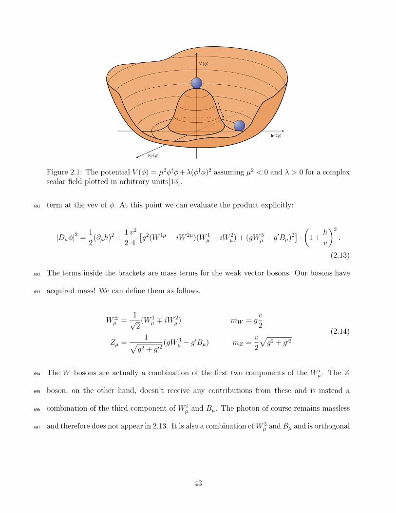
Figure 2.1: The potential V (φ) = µ2φ†φ+λ(φ†φ)2 assuming µ2 < 0 and λ > 0 for a complexscalar field plotted in arbitrary units[13].

term at the vev of φ. At this point we can evaluate the product explicitly:691

|Dµφ|2 =1

2(∂µh)2 +

1

2

v2

4

[g2(W 1µ − iW 2µ)(W 1

µ + iW 2µ) + (gW 3

µ − g′Bµ)2]·(

1 +h

v

)2

.

(2.13)

The terms inside the brackets are mass terms for the weak vector bosons. Our bosons have692

acquired mass! We can define them as follows.693

W±µ =

1√2(W 1

µ ∓ iW 2µ) mW = g

v

2

Zµ =1

√

g2 + g′2(gW 3

µ − g′Bµ) mZ =v

2

√

g2 + g′2

(2.14)

The W bosons are actually a combination of the first two components of the W iµ. The Z694

boson, on the other hand, doesn’t receive any contributions from these and is instead a695

combination of the third component of W iµ and Bµ. The photon of course remains massless696

and therefore does not appear in 2.13. It is also a combination of W 3µ and Bµ and is orthogonal697

43

to Zµ:698

Aµ =1

√

g2 + g′2(g′W 3

µ + gBµ) mγ = 0. (2.15)

We can write the transformation that changes (W 3, B) to (Z,A) as a rotation through the699

weak mixing angle θw:700

Z

A

=

cos θw − sin θw

sin θw cos θw

W 3

B

cos θw =g

√

g2 + g′2, sin θw =

g′

√

g2 + g′2.

(2.16)

Writing the covariant derivatives in terms of the mass eigenstates and identifying the electric701

charge quantum number Q as T 3 + Y and the coefficient of the photon field gg′/√

g2 + g′2702

as e we obtain703

Dµ = ∂µ − ig√2(W µ

+T+ + W µ−T−) − i

g

cos θw

Zµ(T 3 − sin2 θwQ) − ieAµQ. (2.17)

The fermion masses mf are more difficult to include in the Lagrangian because the right-704

and left-handed fields live in different representations. Putting in a mass term in this way705

would violate gauge invariance. Using the Higgs mechanism we can construct these terms by706

contracting the fermion doublets FL with the spinor φ evaluated at the vacuum expectation707

value. New dimensionless coupling constants are required. Again using the unitarity gauge708

we write709

L fermion = −λf FL · φfR

= − v√2λf (1 +

h

v)fLfR

= −mf fLfR(1 +h

v).

(2.18)

44

Our choice of the unitarity gauge obscures some of the underlying mechanics of the scalar710

field that are worth mentioning here. Looking back at Fig. 2.1, the potential takes the shape711

of the bottom of a champagne bottle. At sufficiently high energies the field does not see the712

potential and the system is symmetric. When the system is in its lowest energy state the field713

will ‘settle’ into the the minimum of the potential and the symmetry is broken. We saw that714

small oscillations of the field in the radial direction correspond to the massive Higgs boson.715

We can also consider another type of excitation in this picture: those around the vertical716

axis. Since there are an infinite number of equivalent minima the ground state is degenerate717

and oscillations around the bottom of the bottle move the system to a different, equivalent,718

ground state. These modes correspond to massless Nambu-Goldstone bosons. In EWKSB719

there are three of these Nambu-Goldstone bosons, one for each generator belonging to a720

broken symmetry. Being able to ‘remove’ them from the Lagrangian means that they are not721

physical states but represent extra degrees of freedom. We say that they are “eaten” by the722

weak vector bosons which gain an additional degree of freedom: a longitudinal polarization723

state.724

2.3 Searching for the Higgs Boson725

The mechanism of electroweak symmetry breaking discussed in the previous section predicts726

a massive physical particle which has been named the Higgs boson. In the standard model727

it is a scalar boson with zero spin and no electric or color charges. The only property not728

predicted by the standard model is its mass, mh =√

2µ, which only depends on unknown729

parameters. It couples to all particles roughly in proportion to their mass; very light particles730

couple weakly to the Higgs boson. Unfortunately, most of the particles we can easily create731

45

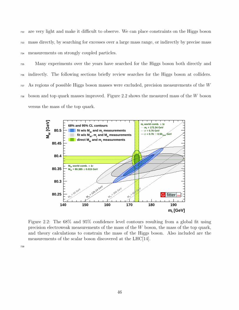
are very light and make it difficult to observe. We can place constraints on the Higgs boson732

mass directly, by searching for excesses over a large mass range, or indirectly by precise mass733

measurements on strongly coupled particles.734

Many experiments over the years have searched for the Higgs boson both directly and735

indirectly. The following sections briefly review searches for the Higgs boson at colliders.736

As regions of possible Higgs boson masses were excluded, precision measurements of the W737

boson and top quark masses improved. Figure 2.2 shows the measured mass of the W boson738

versus the mass of the top quark.

[GeV]tm140 150 160 170 180 190

[GeV

]W

M

80.25

80.3

80.35

80.4

80.45

80.568% and 95% CL contours

measurementst and mW

fit w/o M measurements

H and M

t, m

Wfit w/o M

measurementst and mW

direct M

σ 1± world comb. WM 0.015 GeV± = 80.385 WM

σ 1± world comb. tm = 173.34 GeVtm

= 0.76 GeVσ GeV theo 0.50⊕ = 0.76 σ

= 125.14 GeV

HM = 50 G

eV

HM = 300 G

eV

HM = 600 G

eV

HMG fitter SM

Jul ’14

Figure 2.2: The 68% and 95% confidence level contours resulting from a global fit usingprecision electroweak measurements of the mass of the W boson, the mass of the top quark,and theory calculations to constrain the mass of the Higgs boson. Also included are themeasurements of the scalar boson discovered at the LHC[14].

739

46

2.3.1 LEP Searches740

The Large Electron-Positron (LEP) collider at CERN collided electrons and positrons at741

center of mass energies between 189 GeV and 209 GeV. From 1989 to 2000 the four exper-742

iments at LEP (ALEPH, DELPHI, OPAL, and L3) collected a total of 2461 pb−1 of data.743

The decay branching ratios for the Higgs boson are plotted as a functions of the Higgs bo-744

son mass in Fig 2.3. For a Higgs boson with low mass the primary decay is to pairs of b745

quarks. This was the primary search mode for LEP experiments, but they also performed746

searches that looked for the Higgs boson decaying to pairs of vector bosons and tau leptons.747

The primary production mechanism considered was the Higgs boson produced in association748

with a Z boson in the process e+e− → ZH. The Z boson decayed to either two quarks, two749

charged leptons, or two neutrinos. They were able to set a lower bound on mh of 114.4 GeV750

at the 95% confidence level[15]. Figure 2.4 shows the value of CLs as a function of the tested751

Higgs boson mass. Higgs boson masses are excluded if CLs ≤ 0.05.752

2.3.2 Tevatron Searches753

The Tevatron collider at Fermilab collided protons and antiprotons from 1985 to 2011 at754

center of mass energies up to 1.96 TeV. The experiments at the Tevatron, CDF and D0,755

collected up to 10 fb−1 per experiment. At the center of mass energy of the Tevatron the756

dominant Higgs boson production modes are gluon-gluon fusion, associated V H production,757

vector boson fusion, and associated top quark pair production ttH. Tree-level Feynman758

diagrams for these production modes are given in Fig. 2.5. The production cross sections759

for these processes are plotted over a range of Higgs boson masses in Fig. 2.6. The decay760

branching ratios for the Higgs boson are plotted as a function of the Higgs boson mass in761

47

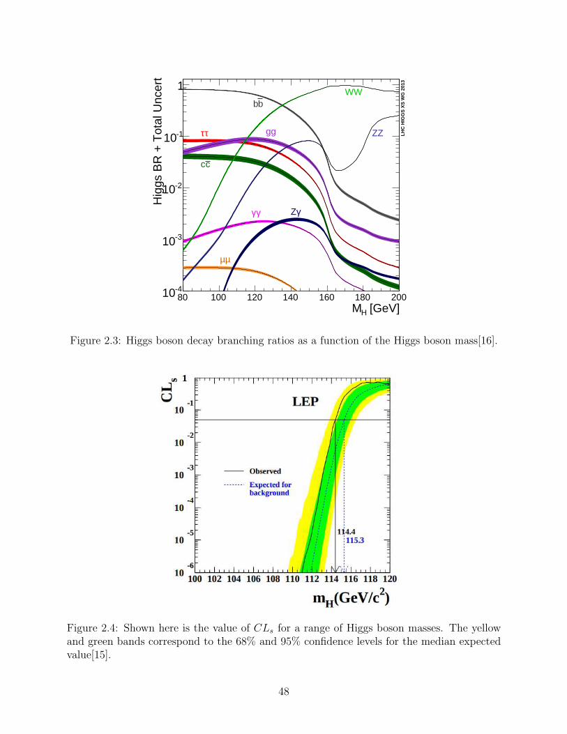
[GeV]HM80 100 120 140 160 180 200

Hig

gs B

R +

Tot

al U

ncer

t

-410

-310

-210

-110

1

LH

C H

IGG

S X

S W

G 2

013

bb

ττ

µµ

cc

gg

γγ γZ

WW

ZZ

Figure 2.3: Higgs boson decay branching ratios as a function of the Higgs boson mass[16].

Figure 2.4: Shown here is the value of CLs for a range of Higgs boson masses. The yellowand green bands correspond to the 68% and 95% confidence levels for the median expectedvalue[15].

48

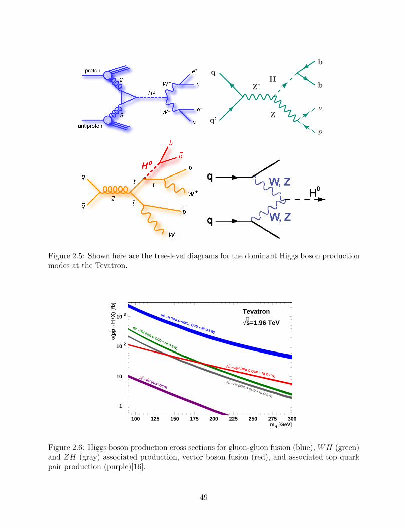
Hq

Zq’

Z∗

b

b

ν

ν

Figure 2.5: Shown here are the tree-level diagrams for the dominant Higgs boson productionmodes at the Tevatron.

1

10

10 2

10 3

100 125 150 175 200 225 250 275 300mH [GeV]

σ(pp

→H

+X)

[fb]

Tevatron

√s

=1.96 TeVpp

–→H (NNLO+NNLL QCD + NLO EW)

pp–→WH (NNLO QCD + NLO EW)

pp–→ZH (NNLO QCD + NLO EW)

pp–→qqH (NNLO QCD + NLO EW)pp–

→tt–H (NLO QCD)

Figure 2.6: Higgs boson production cross sections for gluon-gluon fusion (blue), WH (green)and ZH (gray) associated production, vector boson fusion (red), and associated top quarkpair production (purple)[16].

49

Fig. 2.3. The most dominant decays are to a pair of b quarks up to a Higgs boson mass762

of 135 GeV and to a pair of W bosons at higher masses. The center of mass energy of the763

Tevatron restricts the mass range that can reasonably be probed to ≤ 200 GeV. Searches for764

the Higgs boson at the Tevatron concentrate on the production modes in Fig. 2.6 with the765

Higgs boson decaying to bb or to a pair of W bosons. When searching for the decay H → bb766

we usually consider production modes which have leptons in the final state. Most of the767

interactions that occur at a hadron collider like the Tevatron produce quarks. Final states768

with quarks tend to get overwhelmed by these background interactions. By requiring leptons769

in the final state (which are rarer at hadron colliders) we can limit potential background770

sources.771

The Tevatron was able to exclude Higgs boson masses in the ranges 90 < mH < 109 GeV772

and 149 < mH < 182 GeV[17] at the 95% confidence level when combining all production773

processes and decay modes. For a discussion of the statistical methods employed here please774

refer to Chapter 7. Figure 2.7 shows the observed and expected 95% confidence level upper775

limit divided by the standard model production cross section for a range of Higgs boson776

masses. When combining only V H associated production processes with the Higgs boson777

decaying to two b quarks we also saw evidence6 of a new particle in the mass range 120 <778

mH < 135 which was consistent with the SM Higgs boson[18]. Figure 2.8 shows the expected779

and observed log-likelihood ratio as a function of the Higgs boson mass. The highest local780

significance is at mH = 120 GeV and corresponds to 3.3 s.d. with a global significance of 3.1781

s.d.782

6The terms evidence and observation or discovery have specific connotations in particle physics. Havingevidence of a new particle means that even if the particle doesn’t exist, the probability of getting a resultat least as extreme as the data is 0.3% corresponding to a p-value of 0.003 or a three standard deviation(s.d.) fluctuation above the background expectation. Observation or discovery corresponds to a p-value of

3 × 10−7 or a 5 s.d. fluctuation above the background expectation.

50

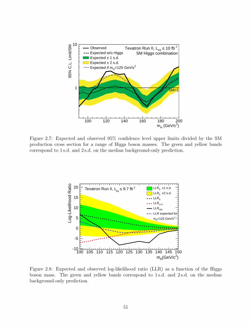
1

10

100 120 140 160 180 200mH (GeV/c2)

95%

C.L

. Lim

it/S

M Tevatron Run II, Lint ≤ 10 fb-1

SM Higgs combinationObservedExpected w/o HiggsExpected ± 1 s.d.Expected ± 2 s.d.Expected if mH=125 GeV/c2

SM=1

Figure 2.7: Expected and observed 95% confidence level upper limits divided by the SMproduction cross section for a range of Higgs boson masses. The green and yellow bandscorrespond to 1 s.d. and 2 s.d. on the median background-only prediction.

)2(GeV/cHm100 105 110 115 120 125 130 135 140 145 150

Log-

Like

lihoo

d R

atio

-10

-5

0

5

10

15

20 1 s.d.± bLLR

2 s.d.± bLLR

bLLR

s+bLLR

obsLLR

LLR expected for2=125 GeV/cHm

-1 9.7 fb≤ int

Tevatron Run II, L

Figure 2.8: Expected and observed log-likelihood ratio (LLR) as a function of the Higgsboson mass. The green and yellow bands correspond to 1 s.d. and 2 s.d. on the medianbackground-only prediction.

51

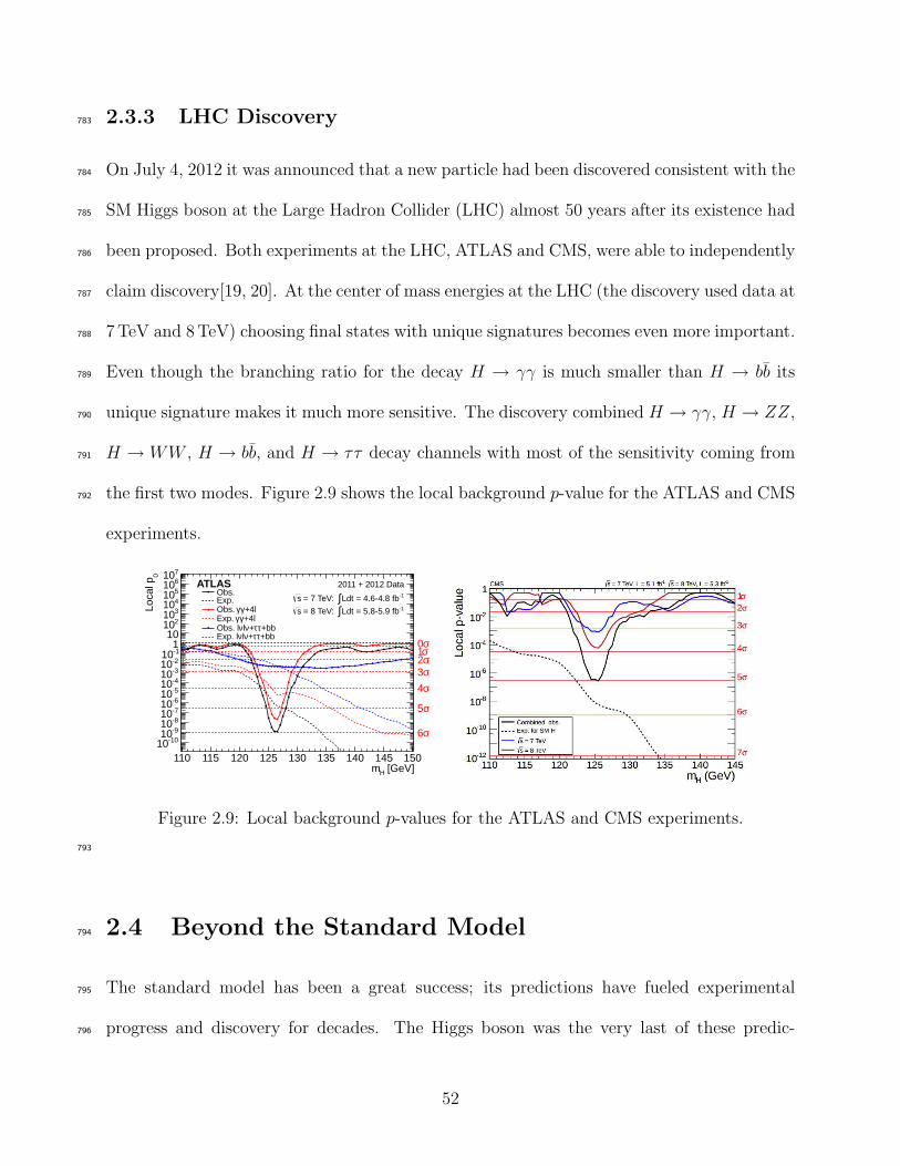
2.3.3 LHC Discovery783

On July 4, 2012 it was announced that a new particle had been discovered consistent with the784

SM Higgs boson at the Large Hadron Collider (LHC) almost 50 years after its existence had785

been proposed. Both experiments at the LHC, ATLAS and CMS, were able to independently786

claim discovery[19, 20]. At the center of mass energies at the LHC (the discovery used data at787

7 TeV and 8 TeV) choosing final states with unique signatures becomes even more important.788

Even though the branching ratio for the decay H → γγ is much smaller than H → bb its789

unique signature makes it much more sensitive. The discovery combined H → γγ, H → ZZ,790

H → WW , H → bb, and H → ττ decay channels with most of the sensitivity coming from791

the first two modes. Figure 2.9 shows the local background p-value for the ATLAS and CMS792

experiments.

[GeV]Hm110 115 120 125 130 135 140 145 150

0Lo

cal p

-1010-910-810-710-610-510-410-310-210-1101

10210310410510610710

Obs. Exp.

+4lγγObs. +4lγγExp.

+bbττ+νlνObs. l+bbττ+νlνExp. l

-1Ldt = 5.8-5.9 fb∫ = 8 TeV: s

-1Ldt = 4.6-4.8 fb∫ = 7 TeV: s

ATLAS

σ0σ1σ2σ3

σ4

σ5

σ6

2011 + 2012 Data

Figure 2.9: Local background p-values for the ATLAS and CMS experiments.

793

2.4 Beyond the Standard Model794

The standard model has been a great success; its predictions have fueled experimental795

progress and discovery for decades. The Higgs boson was the very last of these predic-796

52

tions to be confirmed. However, this does not mean that the standard model is a complete797

theory. There are still open questions and issues that it does not address. Some of these798

problems are inherent, while many are external to the standard model. Below is a list of799

some of the problems from both categories, but it is by no means exhaustive.800

There are issues which are outside the purview of the standard model. These are questions801

for which the standard model simply doesn’t have an answer.802

• Gravity The force of gravity is responsible for the large-scale structure of the universe. It803

is also the force with which we are most familiar yet it is not described by the standard804

model of particle physics. As of this writing there has never been a successful theory805

of quantum gravity.806

• Dark matter and dark energy Cosmological studies of the matter/energy density of807

the universe have shown that the matter described by the standard model constitutes808

less than 5% of the total mass-energy content of the universe. The remaining matter809

content, which contributes ≈ 27% does not interact electromagnetically and remains810

unseen. The remaining mass-energy content is an unknown type of energy which is811

accelerating the expansion of the universe. For this reason we refer to them as dark812

matter and dark energy, respectively. The particles and energies in the SM cannot813

account for these two strange quantities.814

• Matter-antimatter asymmetry The abundance of matter in the universe suggests that815

there was an imbalance of matter and antimatter in the early universe which cannot816

be accounted for in the standard model.817

• Unification In the first epoch of the universe known as the Planck era it is predicted that818

the gravitational force was comparable to all the other forces and that it dominated819

53

matter interactions. The energy scale at which this occurred is referred to as the820

Planck scale and is approximately 1019 GeV. It is theorized that at this scale all the821

forces were different aspects of a single unified force. For this to occur the coupling822

constants for the electroweak and strong forces would become equal at an energy scale823

less than the Planck scale. Unless there is new physics beyond the standard model this824

does not occur.825

Problems inherent in the standard model are either based on disagreements between826

theory and experiment or are philosophical in nature.827

• Neutrino masses In the standard model there is no way to add mass terms for neutrinos828

to the Lagrangian without destroying gauge invariance. The fermion mass terms in829

Eq. 2.18 are constructed using both the left-handed doublet and right-handed singlet830

states of the particles and neutrinos do not exist in a right-handed state. However,831

neutrino experiments have found that neutrinos undergo flavor oscillation – something832

that would not be possible if they did not have mass.833

• Hierarchy problem If unification is possible at the Planck scale the SM offers no expla-834

nation as to why the Planck scale is so much higher than the other energy scales of835

the SM. The electroweak scale is equal to the Higgs boson vacuum expectation value836

of 246 GeV. From this scale all the way up to 1019 GeV is devoid of any interesting837

physics according to the standard model.838

• Fine-tuning Quantum corrections to the third term in Eq. 2.12 produce contributions839

to the Higgs boson mass which are quadratically divergent. They remain finite up840

to the Planck energy scale but the contributions are very large. In order for the841

Higgs boson mass to remain small there must be very precise cancellations to the large842

54

contributions to the Higgs boson mass. This amounts to an unacceptable fine-tuning843

of model parameters. A model which adequately describes reality should not rely on844

a fine-tuning of its parameters.845

All of these problems point to something beyond the standard model. There are many846

theoretical proposals on how to deal with these problems. Some involve extensions to the847

SM which typically include additional SM-like terms to the Lagrangian. These terms of848

course require additional parameters which are not predicted by the standard model. Other849

proposals give the theory a complete overhaul by positing some underlying structure to the850

standard model itself. These theories must reproduce SM predictions as well as provide new851

testable predictions.852

Perhaps one of the most famous beyond-the-SM (BSM) theories is supersymmetry[21, 22].853

Like all of the quantum field theories, supersymmetry is based on an underlying symmetry.854

It posits a symmetry related to particle spin and predicts a fermionic superpartner for every855

boson and a bosonic superpartner for every fermion. If supersymmetry were an unbroken856

symmetry (like the charge symmetry in GWS) then the superpartners would differ only by857

1/2-spin – they would have the same mass and charges as their SM counterparts. Since this858

hasn’t been observed we know that if supersymmetry exists it has to be a broken symmetry.859

2.4.1 BSM Higgs Spin & Parity860

One of the places to look for physics beyond the standard model is one of its newest discov-861

eries: the Higgs boson. If the recently discovered boson is the SM Higgs boson it will have862

zero spin and even parity. There are other possibilities for the spin and parity of the discov-863

ered boson if it is not the SM Higgs boson. Many of these possibilities come from theories864

55

that solve some of the problems with the standard model, most notably the fine-tuning and865

hierarchy problems. A pseudoscalar with JP = 0− is predicted for two Higgs boson doublet866

models of type II[23] such as those found in supersymmetry[24]. Theories postulating extra867

dimensions predict massive particles with tensor couplings and JP = 2+[25, 26]. Knowing868

the spin and parity of the discovered boson or being able to exclude specfic values of JP tells869

us about the structure of the underlying theory. Part II of this Thesis is designed to address870

this issue.871

56

Part II872

Constraints on Models for the Higgs873

Boson874

with Exotic Spin and Parity875

57

Part II provides an in-depth discussion of the data analysis and conclusions. It begins with876

a description of the equipment used to produce, detect, and record the data in Chapter 3.877

Chapter 4 discusses the motivations behind this analysis. It includes an overview of the878

theoretical framework specific to analyzing the spin and parity nature of a Higgs boson879

at the Tevatron. The data and simulated samples used in this analysis are discussed in880

Chapter 5. The data analysis method is described in Chapter 6. Chapter 7 gives an overview881

of the statistical analysis method employed and discusses sources of systematic uncertainties.882

Finally, Chapters 8 and 9 discuss the results of the analysis in detail.883

58

Chapter 3884

Experimental Apparatus885

3.1 Introduction886

Fermi National Accelerator Laboratory1 is a large accelerator complex. Prior to 2008 it was887

the site of the highest-energy particle collisions in the world. That title now belongs to the888

Large Hadron Collider (LHC) near Geneva, Switzerland.889

The lab began life in 1965 with the approval of a high energy physics proposal aimed at890

bringing together experts from universities across the country and the world. The project891

broke ground in 1968 for the first stage of the proton accelerator and was able to reach its892

design collision energy of 200 GeV by early 1972. By the end of 1972 it had doubled its893

energy to 400 GeV. From 1972 to 1985 the accelerator provided beam solely for fixed target894

experiments. During the early ‘80s the lab approved and implemented a plan to use the895

accelerator chain to collide protons and antiprotons. In the fall of 1985 the first proton-896

antiproton collisions were seen at a center of mass energy equal to 1.6 TeV. When collisions897

stopped in the fall of 2011 the center of mass energy was 1.96 TeV.898

The D0 experiment is one of two experiments that detected collisions at Fermilab. The899

D0 Collaboration was founded in 1983, two years before Fermilab saw its first collisions.900

Construction of the 5,000 ton, three-story tall detector that was the centerpiece of the901

experiment was completed in early 1992. It took data until 1996 when it was given a major902

1Located in Batavia, Illinois.

59

upgrade. After the upgrade was complete in 2001 it collected data until collisions were halted903

in the fall of 2011. The collaboration has 68 member institutions from 15 countries and, as904

of 2015, is still analyzing its data.905

3.2 Accelerating Particles at Fermilab906

Figure 3.1 shows a bird’s-eye view of the Fermilab accelerator complex. During the col-907

liding beams era the centerpiece of the Fermilab accelerator complex was the Tevatron, a908

superconducting proton-antiproton synchrotron. This machine was tasked with boosting the909

energy of each beam to their final energy of 980 GeV as well as initiating and maintaining910

collisions at two points around its ring. But the Fermilab accelerator complex is home to a

Figure 3.1: Aerial view of the Fermilab accelerator complex. The large ring is the Tevatron.

911

total of ten accelerators and storage rings. Particles start in one of two Preaccelerators (1 &912

2) where they are accelerated to 750 keV. The first section of the linear accelerator (3), the913

Linac, further accelerates them to 116 MeV while the second section (4) accelerates them to914

400 MeV. After the Linac the particles are sent to the first synchrotron, the Booster (5), and915

60

given a boost up to 8 GeV. From there they move on to the second synchrotron, the Main916

Injector (6), and leave with an energy of 150 GeV. Antiprotons begin in the antiproton source917

and are shuffled to a set of storage rings called the Debuncher (7) and the Accumulator (8)918

which condense and accumulate them. They are then sent to the Recycler (9), a permanent919

magnet storage ring. Eventually, when enough antiprotons have been accumulated, they are920

accelerated in the Main Injector along with the protons to 150 GeV. The Tevatron (10) is921

the final step where the particles reach an energy of 980 GeV.922

Although the Fermilab accelerator chain has gone through many upgrades throughout923

the years (and still continues to do so!), the following sections describe the accelerator chain924

at the time it ceased to operate as a colliding beam accelerator. Section A.1.1 describes the925

path of a proton from the source to the final stage of acceleration. The creation, collection,926

and acceleration of antiprotons is described in Section A.1.2.927

3.3 D0 Detector928

The D0 detector was one of two general-purpose hadron collider detectors situated around929

the Fermilab Tevatron ring. Design began in 1983 during construction of its sister detector,930

the Collider Detector at Fermilab (CDF). This timing motivated a design that was comple-931

mentary to CDF’s strengths and weaknesses, namely one with an enhanced ability to detect932

leptons. Physics goals at the time, reachable at the expected center of mass energy of the933

Tevatron at 2 TeV, included precision measurements of the W± and Z bosons; exploration934

of new phenomena at and above their mass scales, including searches for the top quark;935

and investigation of high transverse momentum pT particles. This required good, full solid936

angle coverage to obtain an accurate measurement of missing transverse energy indicating937

61

the presence of neutrinos. Measurement of high pT particles required the development of a938

sophisticated hadronic calorimeter. All of these specifications were taken into account in the939

design of the D0 detector.940

Construction of the detector was completed in early 1992. It operated during Run I of941

the Tevatron from 1992-1996. During Run I, the Tevatron operated at a center of mass942

energy of 1.8 TeV with six bunches each of protons and antiprotons with a bunch spacing of943

3500 ns. It had a typical peak instantaneous luminosity of 1–2×1031 cm−2s−1. D0 collected944

approximately 120 pb−1 of data and was able to meet most of its physics goals including945

the discovery of the top quark alongside CDF in 1995[27, 28]. From 1996-2001 the Fermilab946

accelerator complex received an upgrade that included the installation of the Main Injector947

and Recycler. During this time the D0 detector was also upgraded with a brand new tracking948

system and electronics to handle the new Tevatron operating conditions. Run II began in949

2001 and ended on September 30, 2011 with the shutdown of the Tevatron. Typical peak950

luminosity near the end of Run II was 2–3×1032 cm−2s−1. The Tevatron operated with three951

trains of twelve bunches each of protons and antiprotons with a bunch spacing of 396 ns.952

The total integrated luminosity delivered by the accelerator during Run II was 11.9 fb−1.953

D0 was able to collect 10.9 fb−1 of data during this time. After data quality cuts the total954

integrated luminosity available for physics analyses was 9.7 fb−1.955

The original detector is described in detail in Ref. [29] with the upgraded detector of956

Run II described in Ref. [30]. An additional upgrade of the tracking system was installed in957

2006 and is described in Ref. [31]. For the purposes of this Thesis the next sections describe958

the detector in the state it was in after the upgrade in 2006.959

The D0 detector is a large machine weighing approximately 5500 tons with approximate960

dimensions 30′×30′×50′. The detector is roughly cylindrically symmetric around the beam961

62

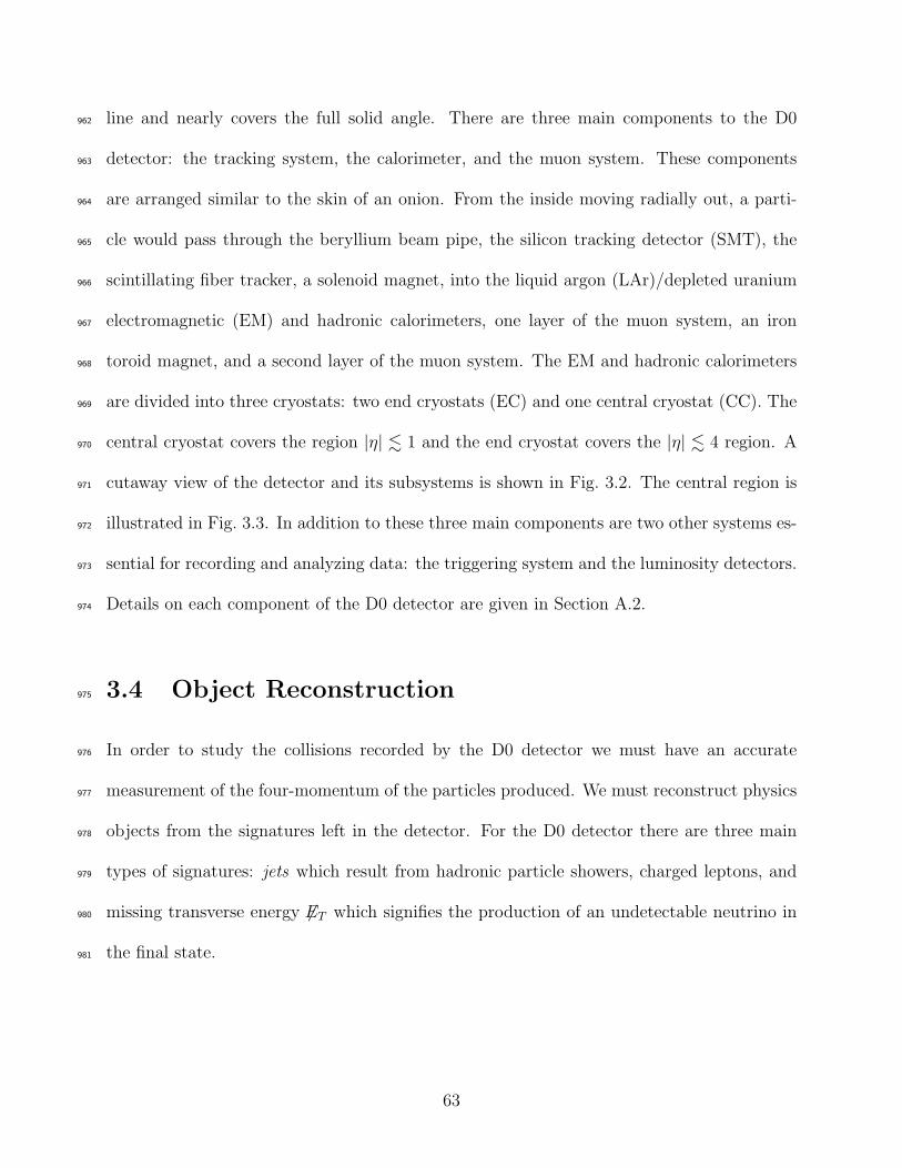
line and nearly covers the full solid angle. There are three main components to the D0962

detector: the tracking system, the calorimeter, and the muon system. These components963

are arranged similar to the skin of an onion. From the inside moving radially out, a parti-964

cle would pass through the beryllium beam pipe, the silicon tracking detector (SMT), the965

scintillating fiber tracker, a solenoid magnet, into the liquid argon (LAr)/depleted uranium966

electromagnetic (EM) and hadronic calorimeters, one layer of the muon system, an iron967

toroid magnet, and a second layer of the muon system. The EM and hadronic calorimeters968

are divided into three cryostats: two end cryostats (EC) and one central cryostat (CC). The969

central cryostat covers the region |η| . 1 and the end cryostat covers the |η| . 4 region. A970

cutaway view of the detector and its subsystems is shown in Fig. 3.2. The central region is971

illustrated in Fig. 3.3. In addition to these three main components are two other systems es-972

sential for recording and analyzing data: the triggering system and the luminosity detectors.973

Details on each component of the D0 detector are given in Section A.2.974

3.4 Object Reconstruction975

In order to study the collisions recorded by the D0 detector we must have an accurate976

measurement of the four-momentum of the particles produced. We must reconstruct physics977

objects from the signatures left in the detector. For the D0 detector there are three main978

types of signatures: jets which result from hadronic particle showers, charged leptons, and979

missing transverse energy 6ET which signifies the production of an undetectable neutrino in980

the final state.981

63

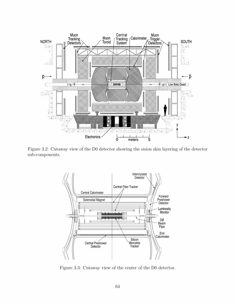
Figure 3.2: Cutaway view of the D0 detector showing the onion skin layering of the detectorsub-components.

Figure 3.3: Cutaway view of the center of the D0 detector.

64

3.4.1 Primary Vertex982

Interactions in the D0 detector do not in general occur in the center of the detector and983

may be offset spatially. Since all other reconstructed objects are defined in reference to the984

interaction point or primary vertex, care must be taken to reconstruct it accurately. Tracks985

with a transverse momentum pT of at least 0.5 GeV and at least two hits in the SMT are986

clustered in 2 cm intervals based on the z coordinates of their distance at closest approach987

from the beamline. These z clusters are then refined by removing outlying tracks with respect988

to the beamline. Selected tracks in a cluster are then fit to a common vertex. Several vertices989

may be found resulting from multiple pp interactions per beam crossing. Many are the result990

of soft pp interactions and some are the result of hard scatter interactions distinguished by991

their higher than average track pT . The vertex that is most likely to have been the result of992

hard scattering is chosen as the primary vertex.993

3.4.2 Jets994

Quarks produced in the interaction will hadronize and produce a hadronic shower of particles995

which deposit most of their energy in the hadronic calorimeter. These energy depositions in996

the calorimeter are referred to as jets. By identifying the shower structure and measuring997

the energy deposited by the jet we can reconstruct position and energy measurements of the998

initial quark. In the following, jets are only reconstructed in the central calorimeter which999

corresponds to the region |η| ≤ 2.5. While there are several good techniques for finding jets in1000

the energy deposition in the calorimeter, we use a simple cone algorithm in this analysis. The1001

Run II Midpoint Cone Algorithm is a clustering algorithm that assigns calorimeter towers1002

to jets within a fixed cone of radius Rcone =√

(∆η)2 + (∆φ)2 = 0.5 in η-φ space. The1003

65

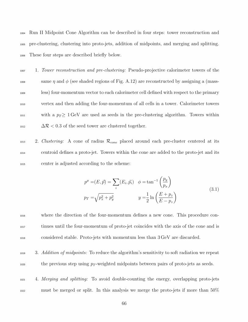
Run II Midpoint Cone Algorithm can be described in four steps: tower reconstruction and1004

pre-clustering, clustering into proto-jets, addition of midpoints, and merging and splitting.1005

These four steps are described briefly below.1006

1. Tower reconstruction and pre-clustering: Pseudo-projective calorimeter towers of the1007

same η and φ (see shaded regions of Fig. A.12) are reconstructed by assigning a (mass-1008

less) four-momentum vector to each calorimeter cell defined with respect to the primary1009

vertex and then adding the four-momentum of all cells in a tower. Calorimeter towers1010

with a pT≥ 1 GeV are used as seeds in the pre-clustering algorithm. Towers within1011

∆R < 0.3 of the seed tower are clustered together.1012

2. Clustering: A cone of radius Rcone placed around each pre-cluster centered at its1013

centroid defines a proto-jet. Towers within the cone are added to the proto-jet and its1014

center is adjusted according to the scheme:1015

pµ =(E, ~p) =∑

i

(Ei, ~pi) φ = tan−1

(py

px

)

pT =√

p2x + p2

y y =1

2ln

(E + pz

E − pz

) (3.1)

where the direction of the four-momentum defines a new cone. This procedure con-1016

tinues until the four-momentum of proto-jet coincides with the axis of the cone and is1017

considered stable. Proto-jets with momentum less than 3 GeV are discarded.1018

3. Addition of midpoints: To reduce the algorithm’s sensitivity to soft radiation we repeat1019

the previous step using pT -weighted midpoints between pairs of proto-jets as seeds.1020

4. Merging and splitting: To avoid double-counting the energy, overlapping proto-jets1021

must be merged or split. In this analysis we merge the proto-jets if more than 50%1022

66

of the pT of the lower energy proto-jet is in the overlap region. Otherwise the cells in1023

the overlap region are assigned to the nearest jet. The four-momenta of the jets are1024

recomputed according to Eqns.3.1 and those with pT < 6 GeV are discarded.1025

To avoid the inclusion of “noisy” jets – jets that contain a large portion of fake calorimeter1026

energy – in physics analyses we impose additional restrictions on the selected jets with the1027

aim of ensuring reasonable energy deposits. We use an algorithm to remove calorimeter cells1028

whose nearest neighbors are unlikely to be from a true jet. The fraction of a jet’s energy1029

deposited in the EM calorimeter must be between 5% and 95% and the energy fraction in1030

the coarse hadronic calorimeter should be less than 40%.1031

3.4.2.1 Heavy-flavor Jets1032

Heavy quarks (specifically charm (c), bottom (b), and top (t)) are important as the decay1033

products of heavy particles such as the W and Higgs bosons and are of interest when looking1034

for physics beyond the standard model. With the exception of the top quark (which decays1035

before it hadronizes), these quarks hadronize and are detected as jets. To a certain degree we1036

are able to distinguish light-flavor from heavy-flavor jets and to a lesser degree between c and1037

b quark jets by their lifetime. Hadrons with charm and bottom content have a relatively long1038

lifetime compared to the top quark and can travel ≈ 3 mm before decaying. This distance1039

is just short enough that the products are still in the tracking volume of the detector.1040

Figure 3.4 depicts an event with a possible heavy-flavor jet. Some characteristics of heavy-1041

flavor jets we might look for in the detector are a displaced vertex and tracks with large1042

impact parameters denoted by d0 in Fig. 3.4. D0 exploits these features using multivariate1043

analysis (MVA) techniques to ‘tag’ jets as originating from b and c quarks. The output of1044

the MVA is a continuum used to identify jets originating from the hadronization of b quarks.1045

67

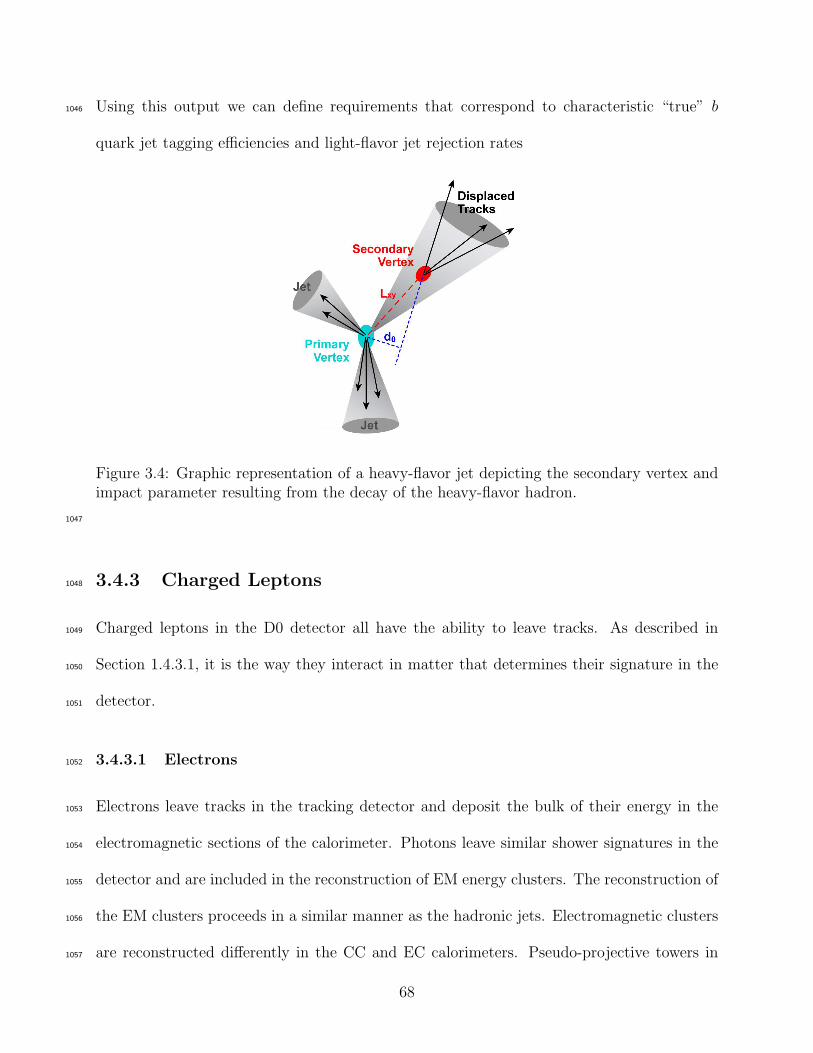
Using this output we can define requirements that correspond to characteristic “true” b1046

quark jet tagging efficiencies and light-flavor jet rejection rates

Figure 3.4: Graphic representation of a heavy-flavor jet depicting the secondary vertex andimpact parameter resulting from the decay of the heavy-flavor hadron.

1047

3.4.3 Charged Leptons1048

Charged leptons in the D0 detector all have the ability to leave tracks. As described in1049

Section 1.4.3.1, it is the way they interact in matter that determines their signature in the1050

detector.1051

3.4.3.1 Electrons1052

Electrons leave tracks in the tracking detector and deposit the bulk of their energy in the1053

electromagnetic sections of the calorimeter. Photons leave similar shower signatures in the1054

detector and are included in the reconstruction of EM energy clusters. The reconstruction of1055

the EM clusters proceeds in a similar manner as the hadronic jets. Electromagnetic clusters1056

are reconstructed differently in the CC and EC calorimeters. Pseudo-projective towers in1057

68

the calorimeter are formed and the transverse energy is summed in the four layers of the EM1058

calorimeter and the first layer of the fine hadronic section of the calorimeter2. Towers with1059

ET < 500 MeV are discarded. In the CC, beginning with the tower with the highest ET1060

adjacent towers within a cone of radius 0.4 in η-φ space are added to form an EM cluster.1061

In the EC, clusters are formed from adjacent towers within a transverse distance of 10 cm1062

from the cell with the highest energy in the third layer of the EM calorimeter. Electrons1063

are distinguished from photons by requiring a track with pT > 1.5 GeV within a ∆η×∆φ =1064

0.05× 0.05 window around the center of the cluster. For clusters in the CC (EC) we require1065

that 97% (90%) of their energy be deposited in a cone of radius√

(∆η)2 + (∆φ)2 = 0.2 in the1066

EM calorimeter layers. In the CC region, a reconstructed isolated track must be associated1067

with the EM cluster. Additional information such as the transverse and longitudinal shower1068

shape, the EM energy fraction, number of hits in the various layers of the tracking detector,1069

and cluster information from the preshower detectors is used to train a multivariate tool1070

called a boosted decision tree (BDT) to identify electrons.1071

3.4.3.2 Muons1072

In contrast to electrons, muons do not produce showers in the EM calorimeter. However,1073

they leave tracks in both the tracking detector and the muon system. Hits in both muon1074

scintillator and wire chambers are used to form track segments in the muon system. These1075

track segments are then matched to tracks in the central tracking detector to form muon1076

candidates. Muon candidates are categorized based on the number of hits in the muon1077

system, the quality of the track reconstruction in the central tracker, and isolation parameters1078

in both the calorimeter and tracking system. The muon system has detectors both inside1079

2The fine hadronic layer is included in the sum to account for leakage of EM showers into the hadronicsection of the calorimeter.

69

and outside the toroid and we require any muon candidates to have hits in both of of these1080

regions, except where the detector support system limits coverage. To reduce the cosmic1081

ray background we use scintillator hit timing information to ensure that hits coincide with1082

a beam crossing.1083

3.4.3.3 Tau Leptons1084

Tau leptons are very short-lived and decay before they can leave a track. Because the tau1085

lepton has a charge of 1, it decays most often to one or three charged particles and some1086

number of neutral particles. Thirty-five percent of the time they decay leptonically to a muon1087

or an electron and two neutrinos. The other 65% of the time they decay hadronically. This1088

analysis does not attempt to reconstruct or reject tau leptons. The effect of their inclusion1089

in the data and simulated samples on the analysis is negligible.1090

3.4.4 Missing Transverse Energy1091

As described in Section 1.4.2.2, colliding beams of particles with equal momentum results in1092

a lab frame that is equivalent to the center of momentum frame and the initial momentum1093

is zero. However, the hard scatter interaction occurs between the partons inside the proton1094

and antiproton. The partons do not carry the full momentum of the proton but instead1095

share it with the other constituents. This means that the total momentum of the interaction1096

is not zero. Fortunately for us the partons carry very little transverse momentum and the1097

total transverse momentum can be assumed to be zero.1098

This is essential to our reconstruction of neutrinos. Neutrinos only interact via the1099

extremely short-range weak force and hence leave the detector without a trace. Their pro-1100

duction in an event must be inferred. We look for an imbalance in the transverse energy of1101

70

the event to identify neutrinos. This “missing” transverse energy or 6ET is calculated from1102

the transverse energy. The transverse energy of individual calorimeter cells in the electro-1103

magnetic and fine hadronic calorimeter sections and clustered energy in the coarse hadronic1104

section are added vectorially and the 6ET is taken to be a vector with the same magnitude1105

with a direction of 180 with respect to the total sum. Any identified muons, which do not1106

leave showers in the calorimeter, are subtracted from the total transverse energy.1107

71

Chapter 41108

Models for the Higgs Boson with1109

Exotic Spin and Parity1110

In Chapter 2 we discussed the possibility of looking for physics beyond the standard model1111

by examining the spin (J) and parity (P ) of the recently discovered Higgs boson. If it is truly1112

the Higgs boson predicted by the SM then it should have JP = 0+. Two of the most highly-1113

motivated BSM JP states are JP = 0− and JP = 2+. The pseudoscalar state JP = 0− can1114

result from two Higgs doublet models of type II[23] such as those found in supersymmetric1115

models[24]. A boson with tensor couplings JP = 2+ can arise in models with extra dimensions1116

such as generic models predicting a bulk Randall-Sundrum graviton[25, 26].1117

The experiments at the LHC have made measurements on the spin and parity of the1118

Higgs boson in the H → WW , H → γγ, and H → ZZ decay channels. The ability of the1119

LHC experiments to distinguish between different JP assignments is based primarily on the1120

angular analysis of the Higgs boson decay products. The measurements have been consistent1121

with the SM JP assignment of JP = 0+ and they have been able to exclude some models1122

with exotic spin and parity[32, 33].1123

The experiments at the Tevatron have found evidence of a particle decaying to two b1124

quarks[18], which is consistent in mass and production rate with the Higgs boson discovered1125

at the LHC[19, 20]. This is unique relative to the LHC measurements which rely on bosonic1126

72

final states. Thus, we are in a unique position to study the spin and parity of this boson1127

in its direct decay to fermions. This is well-motivated because if the Higgs sector is more1128

complex we might expect multiple Higgs bosons which couple separately to fermions and1129

bosons. It is therefore important to study the JP character of the Higgs boson in its decays1130

to both bosons and fermions. The V H associated production channels are among the most1131

sensitive channels at the Tevatron and offer a method for studying the spin and parity of1132

the Higgs boson in a (mostly) model-independent way. In this Thesis we will focus on the1133

WH associated production channel but the general method of analysis is nearly identical1134

to the ZH associated production channels. In Chapter 8 we will discuss the results of the1135

combination of V H channels both at the D0 Collaboration and with the CDF Collaboration.1136

Hq

W±

q’

W±∗

b

b

ν

ℓ±

Figure 4.1: Example tree-level Feynman diagram of the WH associated production channelwith the Higgs boson decaying to a pair of b quarks and the W boson decaying leptonically.

1137

4.1 Threshold Production1138

An example tree-level Feynman diagram of this process is shown in Fig. 4.1. By studying1139

the kinematics of this final state we can distinguish different JP states. At a hadron collider1140

the hard-scatter interaction occurs between the constituent partons of the (anti)proton.1141

73

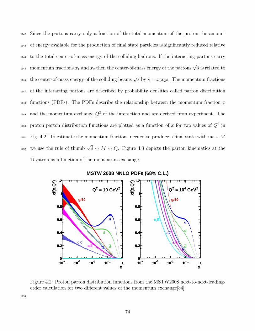
Since the partons carry only a fraction of the total momentum of the proton the amount1142

of energy available for the production of final state particles is significantly reduced relative1143

to the total center-of-mass energy of the colliding hadrons. If the interacting partons carry1144

momentum fractions x1 and x2 then the center-of-mass energy of the partons√

s is related to1145

the center-of-mass energy of the colliding beams√

s by s = x1x2s. The momentum fractions1146

of the interacting partons are described by probability densities called parton distribution1147

functions (PDFs). The PDFs describe the relationship between the momentum fraction x1148

and the momentum exchange Q2 of the interaction and are derived from experiment. The1149

proton parton distribution functions are plotted as a function of x for two values of Q2 in1150

Fig. 4.2. To estimate the momentum fractions needed to produce a final state with mass M1151

we use the rule of thumb√

s ∼ M ∼ Q. Figure 4.3 depicts the parton kinematics at the1152

Tevatron as a function of the momentum exchange.

x-410 -310 -210 -110 1

)2xf

(x,Q

0

0.2

0.4

0.6

0.8

1

1.2

g/10

d

d

u

uss,

cc,

2 = 10 GeV2Q

x-410 -310 -210 -110 1

)2xf

(x,Q

0

0.2

0.4

0.6

0.8

1

1.2

x-410 -310 -210 -110 1

)2xf

(x,Q

0

0.2

0.4

0.6

0.8

1

1.2

g/10

d

d

u

u

ss,

cc,

bb,

2 GeV4 = 102Q

x-410 -310 -210 -110 1

)2xf

(x,Q

0

0.2

0.4

0.6

0.8

1

1.2

MSTW 2008 NNLO PDFs (68% C.L.)

Figure 4.2: Proton parton distribution functions from the MSTW2008 next-to-next-leading-order calculation for two different values of the momentum exchange[34].

1153

74

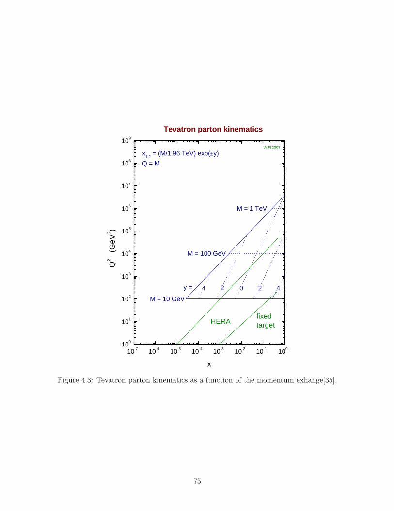
10-7 10-6 10-5 10-4 10-3 10-2 10-1 100100

101

102

103

104

105

106

107

108

109

WJS2008

fixedtargetHERA

x1,2

= (M/1.96 TeV) exp(±y)

Q = M

Tevatron parton kinematics

M = 10 GeV

M = 100 GeV

M = 1 TeV

422 04y =

Q2

(GeV

2 )

x

Figure 4.3: Tevatron parton kinematics as a function of the momentum exhange[35].

75

Producing the WH final state requires an energy of at least 125 + 80 = 205 GeV. The1154

necessary momentum fraction for M2 ≈ 4 × 104 ∼ Q2 can be read from Fig. 4.3. Assuming1155

a rapidity of zero this corresponds to a momentum fraction of approximately x = 0.1. At1156

a momentum fraction x = 0.1 the parton-parton luminosity is near a local maximum and1157

the WH system is almost always produced near threshold. We can define how far the1158

WH system is from threshold as β = 2p/√

s where p is the WH three-momentum in the1159

center-of-mass frame of the colliding beams in units of the center-of-mass energy.1160

4.2 Helicity Amplitudes1161

The method of determining the Higgs boson spin and parity assignments used in this analysis1162

was first described in the context of electron-positron collisions[36], but its application to1163

hadron collisions is straightforward. The form of the production cross section and angular1164

distributions at threshold depend on the JP character of the Higgs boson. Because we are1165

only interested in the behavior of these observables at threshold it is not necessary to know1166

the exact form of the couplings. This allows us to distinguish different JP assignments in1167

a model-independent way. In the following we will work in the helicity formalism (see for1168

example Ref. [37]) which is well-suited for analyzing states with definite spin and parity.1169

Helicity is defined as the dot product of the spin of the particle with the unit vector in1170

the direction of its momentum h = ~S · p1. A massive particle with spin S = J has 2J + 11171

helicity states with values λ = −J, −J + 1, . . . , J . Massless particles on the other hand1172

have only two helicity states λ = ±J due to the fact that there are no components of spin1173

1Here I use S to refer to the spin of the particle to be precise; helicity depends on the spin of the particle~S not the total angular momentum ~J = ~L+ ~S which is defined to be perpendicular to the motion. In collisionphysics we define our axes such that the orbital angular momentum ~L is zero and ~J = ~S.

76

transverse to the direction of motion2. The helicity amplitude A of the W ∗ → WH process1174

with the azimuthal angle set to zero takes the form A ∝ d1M,λ(θ)AλW λH

where d1M,λ(θ) are1175

the Wigner small d matrices which relate a rotated state to an original unrotated state and1176

λ = λW − λH are helicities. The AλW λHare reduced amplitudes which only depend on the1177

helicities of the W and H bosons. The reduced helicity amplitudes are related to states with1178

negative helicity by AλW λH= nHA−λW−λH

. The normality of the Higgs boson nH is defined1179

by nH = (−1)JP . The angular differential cross section is proportional to the square of1180

the helicity amplitudes summed over the final state helicities λH and λW . Performing the1181

summation we obtain:1182

1

σ

dσ

d cos θ=

3

4A2sin2 θ

[|A00|2 + 2|A11|2

]+ (1 + cos2 θ)

[|A01|2 + |A10|2 + |A12|2

]

A2 = |A00|2 + 2|A11|2 + 2|A01|2 + 2|A10|2 + 2|A12|2.(4.1)

Equation 4.1 is the general form for a Higgs boson spin J ≤ 2 and not all terms are1183

nonzero for a specific J . To study the threshold dependence, we can parametrize the reduced1184

amplitudes as a function of β. As an example we can examine the SM case: JP = 0+. The1185

spin of the SM Higgs boson restricts the reduced helicity amplitudes to those of the form1186

AλW 0. The W boson has JP = 1− with helicity values λW = 0, ±1. Only two terms in1187

Eq. 4.1 remain: A00 and A10. Substituting the standard model values A00 = −EW /mW and1188

A10 = −1 and rearranging Eq. 4.1 yields1189

1

σ

dσ

d cos θ=

3

4

β2 sin2 θ + 8m2W /s

β2 + 12m2W /s

. (4.2)

At threshold β → 0 and WH production is isotropic. To leading order, the total cross1190

2Because massless particles travel at the speed of light it is impossible to boost into the rest frame of theparticle; it has no rest frame. You can only measure the spin along its momentum.

77

section near threshold goes as one power of β from the phase space integration. At high1191

boosts (large β) it has a characteristic sin2 θ dependence. Near threshold, where the cross1192

section ∼ β, the production mechanism is thus referred to as s-wave production.1193

To further investigate the implications of Eq. 4.1 we can examine a state with negative1194

normality: JP = 0−. The equation relating reduced helicity amplitudes with positive and1195

negative helicities forbids the A00 term for states with negative normality. Everything else1196

remains the same and this leaves only the A10 term. For a spin and parity assignment of1197

JP = 0−, the A10 term is of the form −iβsa1 where a1 is a coefficient that does not depend on1198

the momenta near threshold. At threshold the production is isotropic and develops a cos2 θ1199

dependence at higher β. The cross section rises as ∼ β3 and the production mechanism1200

is d-wave. Other spin and parity assignments can be examined in the same manner. In1201

general, the cross section rises as the square of the leading order β dependence of the reduced1202

amplitudes plus one factor of β from the phase space integration.1203

4.3 Invariant Mass as a Discrimination Tool1204

The form of the angular distribution above threshold and the β-dependence of the cross1205

section near threshold affect the final state kinematics in observable ways. The angular dis-1206

tribution can be examined by measuring the angular correlations between the decay products1207

in the final state. At the LHC this is the primary method of measuring the spin and parity1208

of the Higgs boson. Compared to the LHC, the Tevatron has a much smaller integrated1209

luminosity and the behavior of the cross section near threshold is more important. The β-1210

dependence of the cross section affects the final state kinematics by enhancing or suppressing1211

the contributions of parton-parton interactions with a particular momentum fraction. As an1212

78

example, consider the case of JP = 0− pseudoscalar versus the SM Higgs boson, JP = 0+.1213

Just above threshold the JP = 0− cross section is heavily suppressed by the β3 dependence1214

compared to the β dependence of the standard model. This pushes production of the WH1215

system to higher energies and, thus, to higher momentum fractions.1216

This effect is observable in the invariant mass distribution of the final state. The square1217

of the invariant mass is defined as the Minkowski inner product of the four-momentum P µPµ.1218

As an invariant it is the same in all reference frames. In the rest frame of the W ∗ boson1219

the invariant mass is simply the mass of the W ∗ boson M . Referring back to Section 4.1 we1220

saw that M2 ∼ x1x2s and threshold production of the WH system requires the momentum1221

fractions to be ∼ 0.1. Larger average momentum fractions will increase the mass of the1222

W ∗ boson and the invariant mass of the system. For WH production the invariant mass as1223

defined in the lab frame is:1224

m =√

(EW + EH)2 − (~pW + ~pH)2. (4.3)

As a proof of concept, the authors of Ref. [38] produced Monte Carlo event samples for1225

ZX → ℓℓbb, WX → ℓνbb, and V X → ννbb production with spin and parity assignments1226

of JP = 0+, 0−, and 2+ and applied the same cuts as the D0 and CDF published analyses1227

of the same production channels. Figure 4.4 shows the invariant mass of the ZX → ℓℓbb1228

final state using D0 cuts. As expected, the JP = 0− state has on average a higher invariant1229

mass. The effect is stronger for the JP = 2+ state because the cross section rises ∼ β5 above1230

threshold, thus forcing x values higher.1231

Because the lifetimes of the W and H bosons are so short we must instead make mea-1232

surements on their decay products. When considering leptonic decays of the W or Z boson1233

79

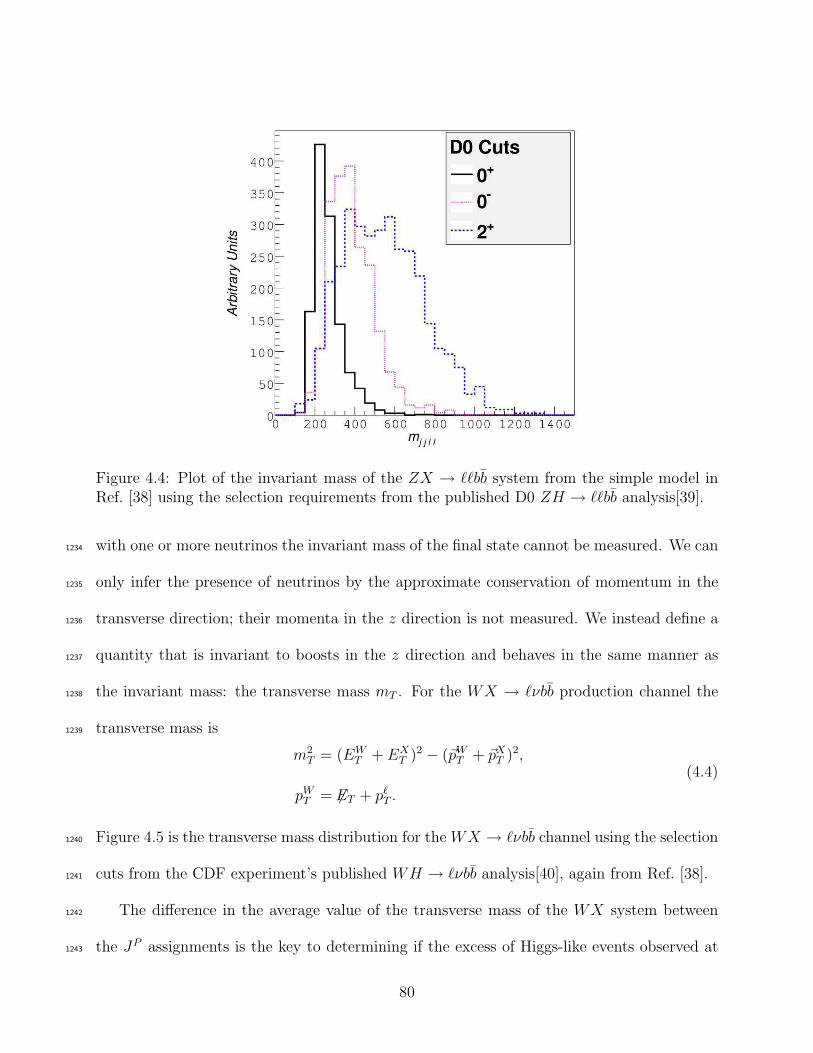
Figure 4.4: Plot of the invariant mass of the ZX → ℓℓbb system from the simple model inRef. [38] using the selection requirements from the published D0 ZH → ℓℓbb analysis[39].

with one or more neutrinos the invariant mass of the final state cannot be measured. We can1234

only infer the presence of neutrinos by the approximate conservation of momentum in the1235

transverse direction; their momenta in the z direction is not measured. We instead define a1236

quantity that is invariant to boosts in the z direction and behaves in the same manner as1237

the invariant mass: the transverse mass mT . For the WX → ℓνbb production channel the1238

transverse mass is1239

m2T = (EW

T + EXT )2 − (~pW

T + ~pXT )2,

pWT = 6ET + pℓ

T .

(4.4)

Figure 4.5 is the transverse mass distribution for the WX → ℓνbb channel using the selection1240

cuts from the CDF experiment’s published WH → ℓνbb analysis[40], again from Ref. [38].1241

The difference in the average value of the transverse mass of the WX system between1242

the JP assignments is the key to determining if the excess of Higgs-like events observed at1243

80

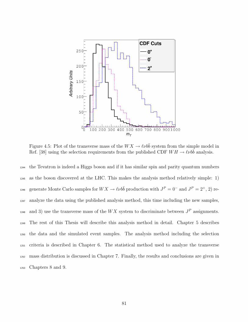
Figure 4.5: Plot of the transverse mass of the WX → ℓνbb system from the simple model inRef. [38] using the selection requirements from the published CDF WH → ℓνbb analysis.

the Tevatron is indeed a Higgs boson and if it has similar spin and parity quantum numbers1244

as the boson discovered at the LHC. This makes the analysis method relatively simple: 1)1245

generate Monte Carlo samples for WX → ℓνbb production with JP = 0− and JP = 2+, 2) re-1246

analyze the data using the published analysis method, this time including the new samples,1247

and 3) use the transverse mass of the WX system to discriminate between JP assignments.1248

The rest of this Thesis will describe this analysis method in detail. Chapter 5 describes1249

the data and the simulated event samples. The analysis method including the selection1250

criteria is described in Chapter 6. The statistical method used to analyze the transverse1251

mass distribution is discussed in Chapter 7. Finally, the results and conclusions are given in1252

Chapters 8 and 9.1253

81

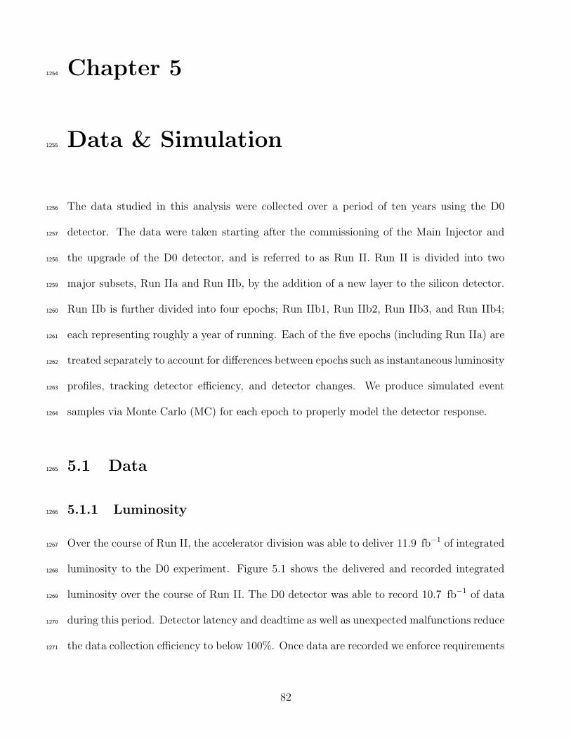
Chapter 51254

Data & Simulation1255

The data studied in this analysis were collected over a period of ten years using the D01256

detector. The data were taken starting after the commissioning of the Main Injector and1257

the upgrade of the D0 detector, and is referred to as Run II. Run II is divided into two1258

major subsets, Run IIa and Run IIb, by the addition of a new layer to the silicon detector.1259

Run IIb is further divided into four epochs; Run IIb1, Run IIb2, Run IIb3, and Run IIb4;1260

each representing roughly a year of running. Each of the five epochs (including Run IIa) are1261

treated separately to account for differences between epochs such as instantaneous luminosity1262

profiles, tracking detector efficiency, and detector changes. We produce simulated event1263

samples via Monte Carlo (MC) for each epoch to properly model the detector response.1264

5.1 Data1265

5.1.1 Luminosity1266

Over the course of Run II, the accelerator division was able to deliver 11.9 fb−1 of integrated1267

luminosity to the D0 experiment. Figure 5.1 shows the delivered and recorded integrated1268

luminosity over the course of Run II. The D0 detector was able to record 10.7 fb−1 of data1269

during this period. Detector latency and deadtime as well as unexpected malfunctions reduce1270

the data collection efficiency to below 100%. Once data are recorded we enforce requirements1271

82

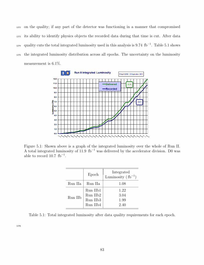
on the quality; if any part of the detector was functioning in a manner that compromised1272

its ability to identify physics objects the recorded data during that time is cut. After data1273

quality cuts the total integrated luminosity used in this analysis is 9.74 fb−1. Table 5.1 shows1274

the integrated luminosity distribution across all epochs. The uncertainty on the luminosity1275

measurement is 6.1%.

Figure 5.1: Shown above is a graph of the integrated luminosity over the whole of Run II.A total integrated luminosity of 11.9 fb−1 was delivered by the accelerator division. D0 wasable to record 10.7 fb−1.

EpochIntegrated

Luminosity ( fb−1)

Run IIa Run IIa 1.08

Run IIb

Run IIb1 1.22Run IIb2 3.04Run IIb3 1.99Run IIb4 2.40

Table 5.1: Total integrated luminosity after data quality requirements for each epoch.

1276

83

5.1.2 Triggers1277

The data sample for this analysis was obtained through the use of specific triggers defined by1278

D0 to capture events with the signature of high-pT electroweak interactions. Of particular1279

importance to this analysis are triggers based on single, charged leptons.1280

For the electron channel we use the logical OR of the single EM and EM+jets trigger1281

suites. Both trigger suites require a good EM trigger object to be above pre-defined thresh-1282

olds and the EM+jets trigger requires at least one high-pT jet. Minimum electron and jet1283

pT thresholds are different for each trigger. The efficiency of these triggers is approximately1284

(90-100)% for the events passing the event selection outlined in Section 6.1 depending on1285

the individual trigger and the location of the electron candidate in the detector volume. We1286

model the trigger response in Monte Carlo by applying a weight to events. The weight is1287

calculated by measuring the trigger efficiency as a function of electron φ, η, and pT .1288

In the muon channel the equivalent trigger suites – single muon and muon+jets – have1289

an efficiency of approximately 70% for our selected events. To increase the acceptance in1290

the muon channel we do not require any specific trigger and instead use the logical OR1291

of all available D0 triggers with the exception of those aimed at identifying heavy-quark1292

jets. The full complement of triggers which contribute to this inclusive event sample is large1293

and varied, making it difficult to model in the Monte Carlo. We therefore take a two-step1294

approach to modeling the muon trigger response. First, we verify good data and simulation1295

agreement for events selected by the well-modeled single muon and muon+jets trigger suites,1296

collectively TµOR. We then compare the data events selected by the inclusive trigger Tincl to1297

the data events selected by TµOR and define a trigger correction for MC intended to account1298

84

for the additional contribution from Tincl:1299

Pcorr =(NData − NMJ)incl − (NData − NMJ)µOR

NMC

. (5.1)

Here NMC is the total number of MC events with trigger efficiency set to 1, NData is the1300

number of data events, and NMJ is the number of multijet events. Multijet events, as1301

detailed in Section 5.3, are estimated from data and do not have this correction applied;1302

their influence on Pcorr is removed by subtracting them from the data events. The final1303

trigger efficiency applied to each MC event is the sum of Pcorr and the efficiency of TµOR1304

with the constraint that the total efficiency must be less than unity. The most significant1305

contributions to Tincl beyond TµOR triggers are based on jets and 6ET . To account for this,1306

the trigger correction Pcorr is parametrized as a function of the scalar sum of the pT of all1307

jets and the 6ET . To account for the changing trigger composition as a function of detector η1308

and the partial muon coverage due to support structures we derive separate corrections for1309

regions in muon η and φ.1310

5.2 Simulated Samples1311

With the exception of the multijet sample, we used Monte Carlo to simulate nearly all SM1312

processes which could result in our final state signature. All simulations use the CTEQ6L1[41]1313

leading-order parton distribution function (PDF) set in the event generation. Parton show-1314

ering and hadronization is done with pythia[42] for all MC samples. Events are processed1315

through a full detector simulation using geant[43]. To simulate the operating conditions of1316

the detector such as residual signals from the previous beam crossing (referred to as pile-up),1317

85

noise in the detector, and additional pp interactions (or underlying events) we overlay events1318

from randomly selected beam crossings with the same luminosity. Finally, the simulated1319

events are put through the same reconstruction process as data.1320

5.2.1 Signals1321

To test the compatibility of models for a Higgs boson with non-SM JP assignments with data1322

we study the WH → ℓνbb process. We include the ZH → ℓℓbb process in our signal samples1323

to account for scenarios where only one of the leptons is identified and the other contributes1324

to the 6ET . All samples have been generated for a Higgs mass mH of 125 GeV. The SM1325

Higgs boson signal processes, which have JP = 0+, are generated using pythia. Both non-1326

SM Higgs boson signals, the pseudoscalar JP = 0− and the graviton-like JP = 2+ signals,1327

are generated using madgraph[44]. We use a Randall-Sundrum (RS) extra-dimensional1328

model[25, 26] which has a JP = 2+ particle with graviton-like couplings to simulate a1329

non-SM JP = 2+ Higgs boson. A generic model of this type has been implemented in1330

madgraph[45, 46]. To generate events using this model we assign the JP = 2+ particle a1331

mass of 125 GeV and specify the production mechanism and final state. In addition to the1332

models available in madgraph, it is possible to implement user-defined models. The model1333

used for the generation of events with a non-SM JP = 0− Higgs boson was written by the1334

authors of Reference [38]. We have verified that the SM Higgs boson sample generated with1335

pythia agrees with a SM Higgs boson sample produced with madgraph.1336

All signal samples are normalized to the cross section times decay branching ratio as1337

predicted by the standard model. The signal cross sections are calculated at next-to-next-1338

to-leading order (NNLO) using the MSTW2008 NNLO PDF set[34]. We use hdecay[47] to1339

obtain the decay branching fraction for the Higgs boson. Table 5.2 lists all the signal pro-1340

86

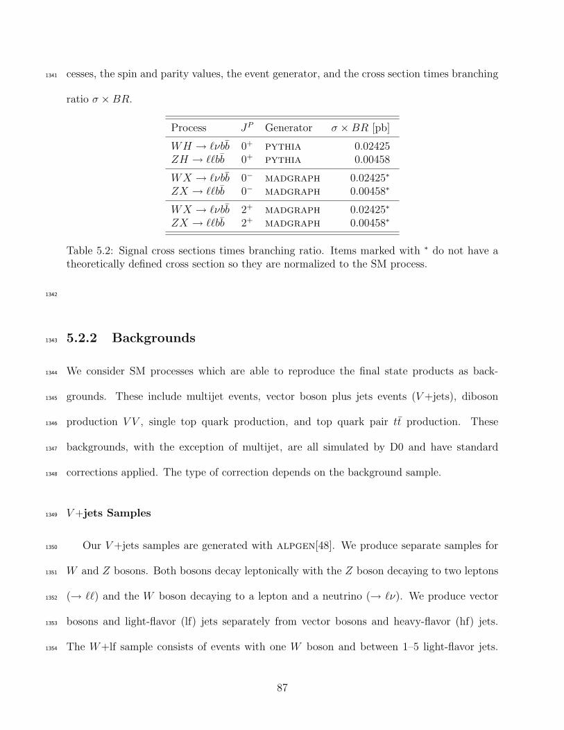
cesses, the spin and parity values, the event generator, and the cross section times branching1341

ratio σ × BR.

Process JP Generator σ × BR [pb]

WH → ℓνbb 0+ pythia 0.02425ZH → ℓℓbb 0+ pythia 0.00458

WX → ℓνbb 0− madgraph 0.02425∗

ZX → ℓℓbb 0− madgraph 0.00458∗

WX → ℓνbb 2+ madgraph 0.02425∗

ZX → ℓℓbb 2+ madgraph 0.00458∗

Table 5.2: Signal cross sections times branching ratio. Items marked with ∗ do not have atheoretically defined cross section so they are normalized to the SM process.

1342

5.2.2 Backgrounds1343

We consider SM processes which are able to reproduce the final state products as back-1344

grounds. These include multijet events, vector boson plus jets events (V +jets), diboson1345

production V V , single top quark production, and top quark pair tt production. These1346

backgrounds, with the exception of multijet, are all simulated by D0 and have standard1347

corrections applied. The type of correction depends on the background sample.1348

V +jets Samples1349

Our V +jets samples are generated with alpgen[48]. We produce separate samples for1350

W and Z bosons. Both bosons decay leptonically with the Z boson decaying to two leptons1351

(→ ℓℓ) and the W boson decaying to a lepton and a neutrino (→ ℓν). We produce vector1352

bosons and light-flavor (lf) jets separately from vector bosons and heavy-flavor (hf) jets.1353

The W+lf sample consists of events with one W boson and between 1–5 light-flavor jets.1354

87

Heavy-flavor jets are defined as having b or c quark content and the W+hf sample consists1355

of one W boson, two b (c) jets, and 1–3 light-flavor jets. The Z+lf and Z+hf samples are1356

generated in a similar manner with one Z boson and 1–3 light-flavor jets or two b (c) jets1357

and 1–2 light-flavor jets, respectively. The Z+jets samples are produced in four regions1358

depending on the mass of the Z boson to increase statistics.1359

We reweight our V +jets samples to account for known issues (see for example Ref. [49]) in1360

alpgen leading to incorrect modeling of certain kinematic distributions. The reweightings1361

are designed to correct the shape of the distribution without affecting the overall normal-1362

ization. To minimize contamination from signal we derive the correction before events are1363

b-tagged. Corrections are derived in event samples selected with the muon+jets triggers by a1364

direct comparison between V +jets MC and data with all non-V +jets backgrounds subtracted1365

and are applied to both electrons and muons. We correct the η distribution of the two high-1366

est pT jets for both W+jets and Z+jets events. The lepton η distribution in W+jets events1367

is also corrected. Discrepancies in the transverse momentum of the W boson pWT and the jet1368

separation in η-φ space ∆R(j1, j2) are correlated and a two-dimensional correction is derived.1369

The pWT reweighting is only applied to W+jets events while the ∆R(j1, j2) reweighting is1370

applied to all V +jets events. The V +jets sample and the multijet sample are normalized to1371

data after the event selection. A simultaneous fit of the V +jets and multijet samples to data1372

with all other SM backgrounds subtracted is performed in the mWT distribution. Tables 5.31373

and 5.4 summarize the events generated for the V +jets sample.1374

Diboson V V Samples1375

Diboson processes include WW , ZZ, or WZ production where one weak vector boson1376

decays leptonically and one decays hadronically. All diboson processes are generated with1377

88

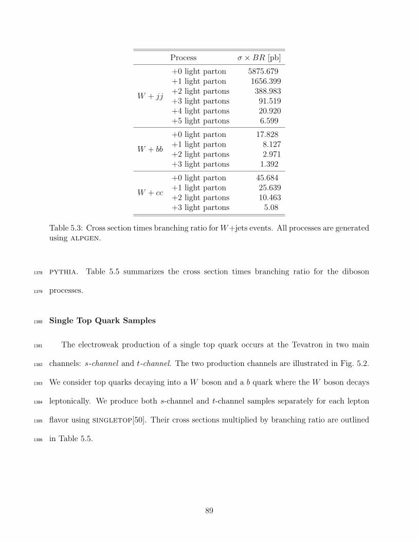
Process σ × BR [pb]

W + jj

+0 light parton 5875.679+1 light parton 1656.399+2 light partons 388.983+3 light partons 91.519+4 light partons 20.920+5 light partons 6.599

W + bb

+0 light parton 17.828+1 light parton 8.127+2 light partons 2.971+3 light partons 1.392

W + cc

+0 light parton 45.684+1 light parton 25.639+2 light partons 10.463+3 light partons 5.08

Table 5.3: Cross section times branching ratio for W+jets events. All processes are generatedusing alpgen.

pythia. Table 5.5 summarizes the cross section times branching ratio for the diboson1378

processes.1379

Single Top Quark Samples1380

The electroweak production of a single top quark occurs at the Tevatron in two main1381

channels: s-channel and t-channel. The two production channels are illustrated in Fig. 5.2.1382

We consider top quarks decaying into a W boson and a b quark where the W boson decays1383

leptonically. We produce both s-channel and t-channel samples separately for each lepton1384

flavor using singletop[50]. Their cross sections multiplied by branching ratio are outlined1385

in Table 5.5.1386

89

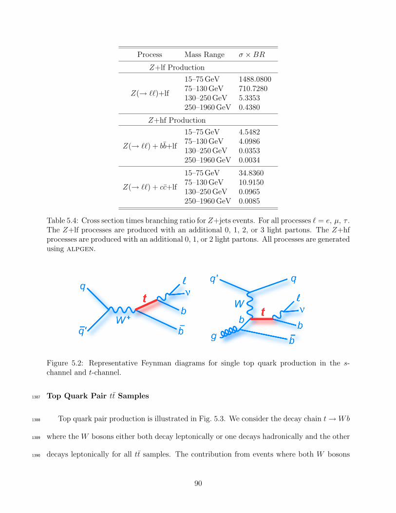
Process Mass Range σ × BR

Z+lf Production

Z(→ ℓℓ)+lf

15–75 GeV 1488.080075–130 GeV 710.7280130–250 GeV 5.3353250–1960 GeV 0.4380

Z+hf Production

Z(→ ℓℓ) + bb+lf

15–75 GeV 4.548275–130 GeV 4.0986130–250 GeV 0.0353250–1960 GeV 0.0034

Z(→ ℓℓ) + cc+lf

15–75 GeV 34.836075–130 GeV 10.9150130–250 GeV 0.0965250–1960 GeV 0.0085

Table 5.4: Cross section times branching ratio for Z+jets events. For all processes ℓ = e, µ, τ .The Z+lf processes are produced with an additional 0, 1, 2, or 3 light partons. The Z+hfprocesses are produced with an additional 0, 1, or 2 light partons. All processes are generatedusing alpgen.

Figure 5.2: Representative Feynman diagrams for single top quark production in the s-channel and t-channel.

Top Quark Pair tt Samples1387

Top quark pair production is illustrated in Fig. 5.3. We consider the decay chain t → Wb1388

where the W bosons either both decay leptonically or one decays hadronically and the other1389

decays leptonically for all tt samples. The contribution from events where both W bosons1390

90

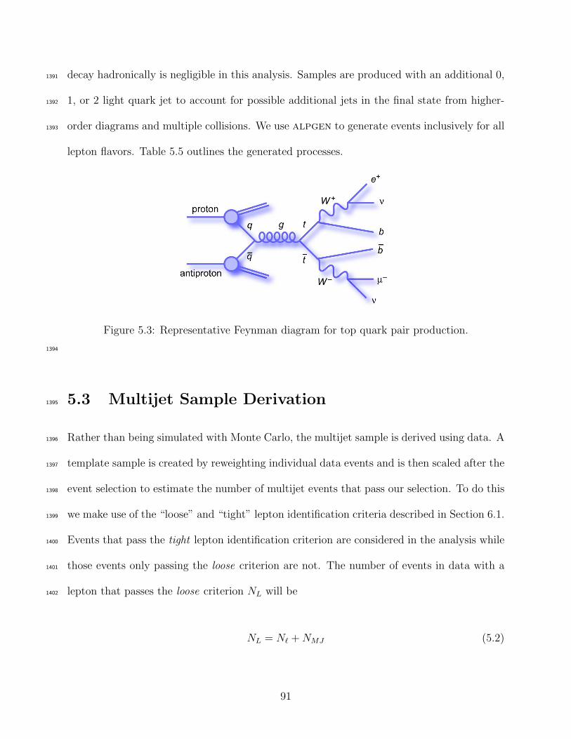
decay hadronically is negligible in this analysis. Samples are produced with an additional 0,1391

1, or 2 light quark jet to account for possible additional jets in the final state from higher-1392

order diagrams and multiple collisions. We use alpgen to generate events inclusively for all1393

lepton flavors. Table 5.5 outlines the generated processes.

Figure 5.3: Representative Feynman diagram for top quark pair production.

1394

5.3 Multijet Sample Derivation1395

Rather than being simulated with Monte Carlo, the multijet sample is derived using data. A1396

template sample is created by reweighting individual data events and is then scaled after the1397

event selection to estimate the number of multijet events that pass our selection. To do this1398

we make use of the “loose” and “tight” lepton identification criteria described in Section 6.1.1399

Events that pass the tight lepton identification criterion are considered in the analysis while1400

those events only passing the loose criterion are not. The number of events in data with a1401

lepton that passes the loose criterion NL will be1402

NL = Nℓ + NMJ (5.2)

91

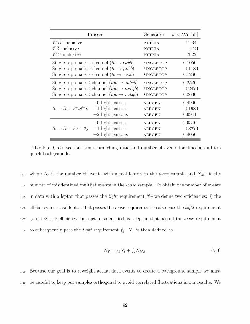
Process Generator σ × BR [pb]

WW inclusive pythia 11.34ZZ inclusive pythia 1.20WZ inclusive pythia 3.22

Single top quark s-channel (tb → eνbb) singletop 0.1050Single top quark s-channel (tb → µνbb) singletop 0.1180Single top quark s-channel (tb → τνbb) singletop 0.1260

Single top quark t-channel (tqb → eνbqb) singletop 0.2520Single top quark t-channel (tqb → µνbqb) singletop 0.2470Single top quark t-channel (tqb → τνbqb) singletop 0.2630

tt → bb + ℓ+νℓ−ν+0 light parton alpgen 0.4900+1 light parton alpgen 0.1980+2 light partons alpgen 0.0941

tt → bb + ℓν + 2j+0 light parton alpgen 2.0340+1 light parton alpgen 0.8270+2 light partons alpgen 0.4050

Table 5.5: Cross sections times branching ratio and number of events for diboson and topquark backgrounds.

where Nℓ is the number of events with a real lepton in the loose sample and NMJ is the1403

number of misidentified multijet events in the loose sample. To obtain the number of events1404

in data with a lepton that passes the tight requirement NT we define two efficiencies: i) the1405

efficiency for a real lepton that passes the loose requirement to also pass the tight requirement1406

ǫℓ and ii) the efficiency for a jet misidentified as a lepton that passed the loose requirement1407

to subsequently pass the tight requirement fj. NT is then defined as1408

NT = ǫℓNℓ + fjNMJ . (5.3)

Because our goal is to reweight actual data events to create a background sample we must1409

be careful to keep our samples orthogonal to avoid correlated fluctuations in our results. We1410

92

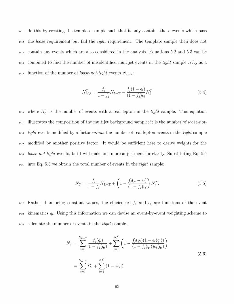
do this by creating the template sample such that it only contains those events which pass1411

the loose requirement but fail the tight requirement. The template sample then does not1412

contain any events which are also considered in the analysis. Equations 5.2 and 5.3 can be1413

combined to find the number of misidentified multijet events in the tight sample NTMJ as a1414

function of the number of loose-not-tight events NL−T :1415

NTMJ =

fj

1 − fj

NL−T − fj(1 − ǫℓ)

(1 − fj)ǫℓ

NTℓ (5.4)

where NTℓ is the number of events with a real lepton in the tight sample. This equation1416

illustrates the composition of the multijet background sample; it is the number of loose-not-1417

tight events modified by a factor minus the number of real lepton events in the tight sample1418

modified by another positive factor. It would be sufficient here to derive weights for the1419

loose-not-tight events, but I will make one more adjustment for clarity. Substituting Eq. 5.41420

into Eq. 5.3 we obtain the total number of events in the tight sample:1421

NT =fj

1 − fj

NL−T +

(

1 − fj(1 − ǫℓ)

(1 − fj)ǫℓ

)

NTℓ . (5.5)

Rather than being constant values, the efficiencies fj and ǫℓ are functions of the event1422

kinematics qi. Using this information we can devise an event-by-event weighting scheme to1423

calculate the number of events in the tight sample.1424

NT =

NL−T∑

i=1

fj(qi)

1 − fj(qi)+

NTℓ∑

i=1

(

1 − fj(qi)(1 − ǫℓ(qi))

(1 − fj(qi))ǫℓ(qi)

)

=

NL−T∑

i=1

Ωi +

NTℓ∑

i=1

(1 − |ωi|)

(5.6)

93

The weights Ωi and 1− |ωi| are applied to the loose-not-tight sample and real lepton events1425

in the tight sample, respectively. Real lepton events in the tight sample are a source of signal1426

contamination in the multijet background sample. The weight applied to these events is1427

expected to be a second-order effect and as such is only applied to the dominant source of1428

real leptons in the tight sample: V +jets events.1429

The lepton efficiencies ǫℓ are derived from a sample of Z/γ∗ → ℓℓ events and are functions1430

of lepton pT . The jet efficiencies fj are calculated in an event sample with 5 < 6ET < 15 GeV1431

and no triangle cut (see Section 6.1) meant to reduce the multijet background. All other1432

event selection criteria are applied. In the electron channel the efficiency is parametrized1433

as a function of detector |η| in regions of electron pT and the minimum φ angle between1434

the vector 6ET and jet ∆φ(6ET , jet). The efficiency in the muon channel is parametrized as a1435

function of muon pT in regions of detector |η| and ∆φ(6ET , µ).1436

94

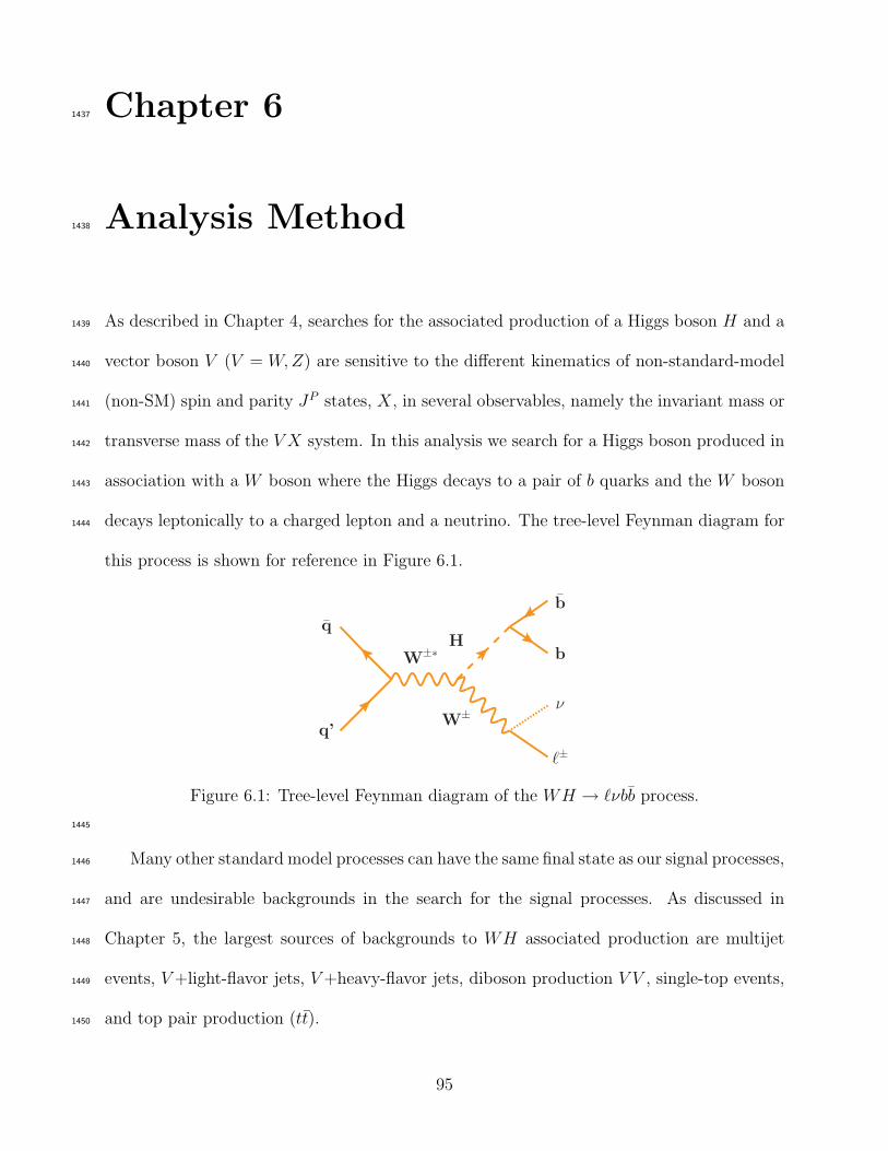
Chapter 61437

Analysis Method1438

As described in Chapter 4, searches for the associated production of a Higgs boson H and a1439

vector boson V (V = W,Z) are sensitive to the different kinematics of non-standard-model1440

(non-SM) spin and parity JP states, X, in several observables, namely the invariant mass or1441

transverse mass of the V X system. In this analysis we search for a Higgs boson produced in1442

association with a W boson where the Higgs decays to a pair of b quarks and the W boson1443

decays leptonically to a charged lepton and a neutrino. The tree-level Feynman diagram for1444

this process is shown for reference in Figure 6.1.

Hq

W±

q’

W±∗

b

b

ν

ℓ±

Figure 6.1: Tree-level Feynman diagram of the WH → ℓνbb process.

1445

Many other standard model processes can have the same final state as our signal processes,1446

and are undesirable backgrounds in the search for the signal processes. As discussed in1447

Chapter 5, the largest sources of backgrounds to WH associated production are multijet1448

events, V +light-flavor jets, V +heavy-flavor jets, diboson production V V , single-top events,1449

and top pair production (tt).1450

95

In any search it is necessary to be able to discriminate between signal and background1451

events through event selection and background rejection. Careful event selection maximizes1452

the number of signal events included while minimizing the amount of background. Section 6.11453

describes the event selection in detail. Signals can be further discriminated from backgrounds1454

by training a multivariate analysis tool to differentiate between signal and background events1455

using many observables. We use a Boosted Decision Tree (BDT) as described in Section 6.21456

for this purpose. The final observable, the transverse mass of the WX system, is discussed1457

in Section 6.3.1458

6.1 Event Selection1459

With the goal of reconstructing the W and Higgs bosons, we search for events with one1460

charged lepton (e or µ)1, significant missing transverse energy, and at least two jets. Ad-1461

ditional requirements on the event and objects within the event are applied to help reject1462

backgrounds and aid in object reconstruction. The event selection used in this analysis is1463

described in the following. Table 6.1 summarizes the event selection.1464

6.1.1 Reconstructing the W Boson1465

To reconstruct the W boson we require exactly one electron or muon in the event along with1466

significant 6ET . Electrons and muons are identified following the prescription in Section 3.4.1467

The 6ET is calculated as described in Section 3.4. Our samples are divided into channels based1468

on the flavor of the identified lepton. In this analysis two sets of identification requirements1469

are applied to leptons in order to form “loose” and “tight” lepton samples. The loose lepton1470

1We do not select tau leptons directly and their contribution to the event sample is small.

96

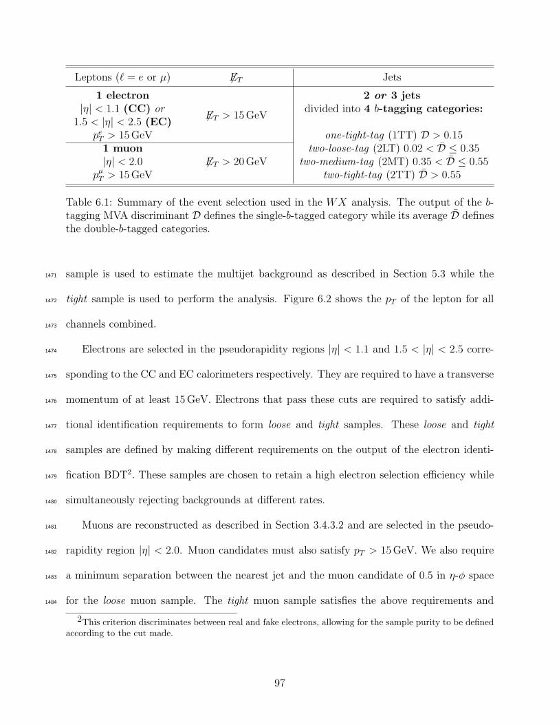
Leptons (ℓ = e or µ) 6ET Jets

1 electron

6ET > 15 GeV

2 or 3 jets|η| < 1.1 (CC) or divided into 4 b-tagging categories:

1.5 < |η| < 2.5 (EC)pe

T > 15 GeV one-tight-tag (1TT) D > 0.151 muon

6ET > 20 GeVtwo-loose-tag (2LT) 0.02 < D ≤ 0.35

|η| < 2.0 two-medium-tag (2MT) 0.35 < D ≤ 0.55pµ

T > 15 GeV two-tight-tag (2TT) D > 0.55

Table 6.1: Summary of the event selection used in the WX analysis. The output of the b-tagging MVA discriminant D defines the single-b-tagged category while its average D definesthe double-b-tagged categories.

sample is used to estimate the multijet background as described in Section 5.3 while the1471

tight sample is used to perform the analysis. Figure 6.2 shows the pT of the lepton for all1472

channels combined.1473

Electrons are selected in the pseudorapidity regions |η| < 1.1 and 1.5 < |η| < 2.5 corre-1474

sponding to the CC and EC calorimeters respectively. They are required to have a transverse1475

momentum of at least 15 GeV. Electrons that pass these cuts are required to satisfy addi-1476

tional identification requirements to form loose and tight samples. These loose and tight1477

samples are defined by making different requirements on the output of the electron identi-1478

fication BDT2. These samples are chosen to retain a high electron selection efficiency while1479

simultaneously rejecting backgrounds at different rates.1480

Muons are reconstructed as described in Section 3.4.3.2 and are selected in the pseudo-1481

rapidity region |η| < 2.0. Muon candidates must also satisfy pT > 15 GeV. We also require1482

a minimum separation between the nearest jet and the muon candidate of 0.5 in η-φ space1483

for the loose muon sample. The tight muon sample satisfies the above requirements and1484

2This criterion discriminates between real and fake electrons, allowing for the sample purity to be definedaccording to the cut made.

97

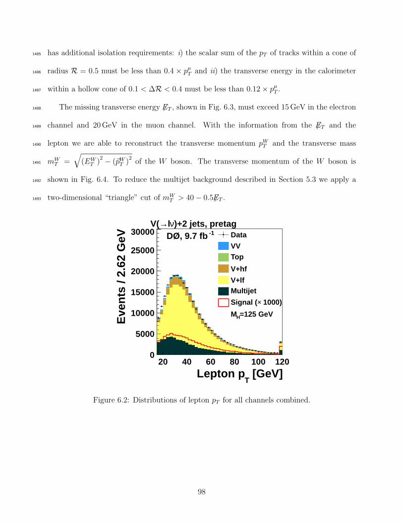
has additional isolation requirements: i) the scalar sum of the pT of tracks within a cone of1485

radius R = 0.5 must be less than 0.4 × pµT and ii) the transverse energy in the calorimeter1486

within a hollow cone of 0.1 < ∆R < 0.4 must be less than 0.12 × pµT .1487

The missing transverse energy 6ET , shown in Fig. 6.3, must exceed 15 GeV in the electron1488

channel and 20 GeV in the muon channel. With the information from the 6ET and the1489

lepton we are able to reconstruct the transverse momentum pWT and the transverse mass1490

mWT =

√

(EWT )

2 − (~pWT )

2of the W boson. The transverse momentum of the W boson is1491

shown in Fig. 6.4. To reduce the multijet background described in Section 5.3 we apply a1492

two-dimensional “triangle” cut of mWT > 40 − 0.56ET .1493

[GeV]T

Lepton p20 40 60 80 100 120

Eve

nts

/ 2.6

2 G

eV

0

5000

10000

15000

20000

25000

30000 -1DØ, 9.7 fb)+2 jets, pretagνl→V(

Data

VVTop

V+hf

V+lfMultijet

1000)×Signal (

=125 GeVHM

Figure 6.2: Distributions of lepton pT for all channels combined.

98

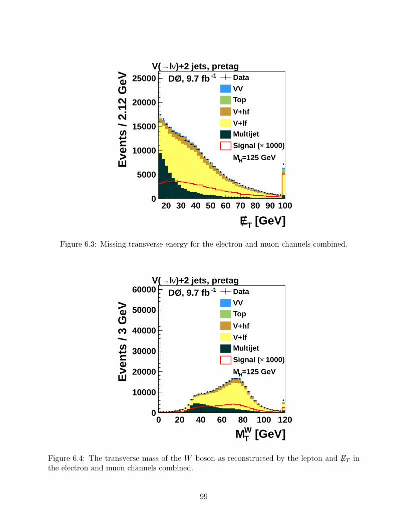
[GeV]TE20 30 40 50 60 70 80 90 100

Eve

nts

/ 2.1

2 G

eV

0

5000

10000

15000

20000

25000 -1DØ, 9.7 fb)+2 jets, pretagνl→V(

Data

VVTop

V+hf

V+lfMultijet

1000)×Signal (

=125 GeVHM

Figure 6.3: Missing transverse energy for the electron and muon channels combined.

[GeV]WTM

0 20 40 60 80 100 120

Eve

nts

/ 3 G

eV

0

10000

20000

30000

40000

50000

60000 -1DØ, 9.7 fb)+2 jets, pretagνl→V(

Data

VVTop

V+hf

V+lfMultijet

1000)×Signal (

=125 GeVHM

Figure 6.4: The transverse mass of the W boson as reconstructed by the lepton and 6ET inthe electron and muon channels combined.

99

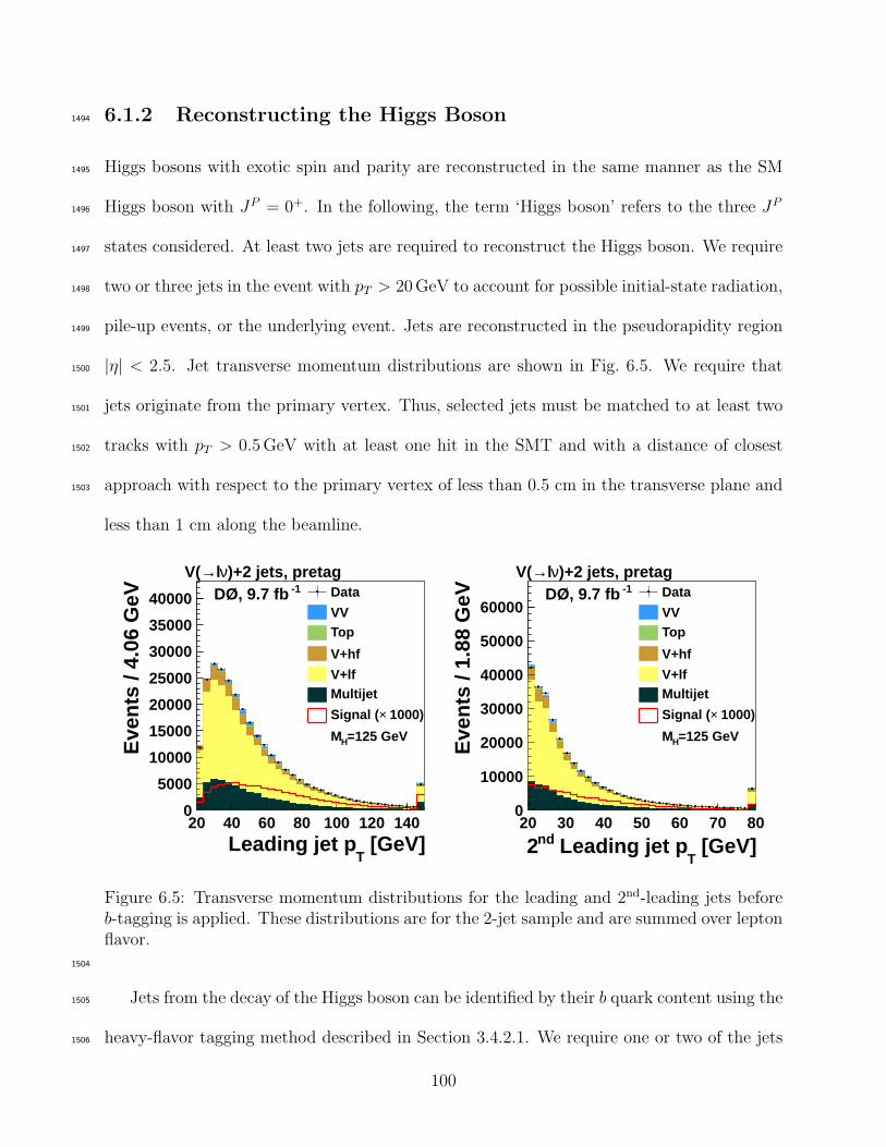
6.1.2 Reconstructing the Higgs Boson1494

Higgs bosons with exotic spin and parity are reconstructed in the same manner as the SM1495

Higgs boson with JP = 0+. In the following, the term ‘Higgs boson’ refers to the three JP1496

states considered. At least two jets are required to reconstruct the Higgs boson. We require1497

two or three jets in the event with pT > 20 GeV to account for possible initial-state radiation,1498

pile-up events, or the underlying event. Jets are reconstructed in the pseudorapidity region1499

|η| < 2.5. Jet transverse momentum distributions are shown in Fig. 6.5. We require that1500

jets originate from the primary vertex. Thus, selected jets must be matched to at least two1501

tracks with pT > 0.5 GeV with at least one hit in the SMT and with a distance of closest1502

approach with respect to the primary vertex of less than 0.5 cm in the transverse plane and1503

less than 1 cm along the beamline.

[GeV]T

Leading jet p20 40 60 80 100 120 140

Eve

nts

/ 4.0

6 G

eV

0

5000

10000

15000

20000

25000

30000

35000

40000 -1DØ, 9.7 fb

)+2 jets, pretagνl→V(Data

VVTop

V+hf

V+lfMultijet

1000)×Signal (

=125 GeVHM

[GeV]T

Leading jet pnd220 30 40 50 60 70 80

Eve

nts

/ 1.8

8 G

eV

0

10000

20000

30000

40000

50000

60000 -1DØ, 9.7 fb

)+2 jets, pretagνl→V(Data

VVTop

V+hf

V+lfMultijet

1000)×Signal (

=125 GeVHM

Figure 6.5: Transverse momentum distributions for the leading and 2nd-leading jets beforeb-tagging is applied. These distributions are for the 2-jet sample and are summed over leptonflavor.

1504

Jets from the decay of the Higgs boson can be identified by their b quark content using the1505

heavy-flavor tagging method described in Section 3.4.2.1. We require one or two of the jets1506

100

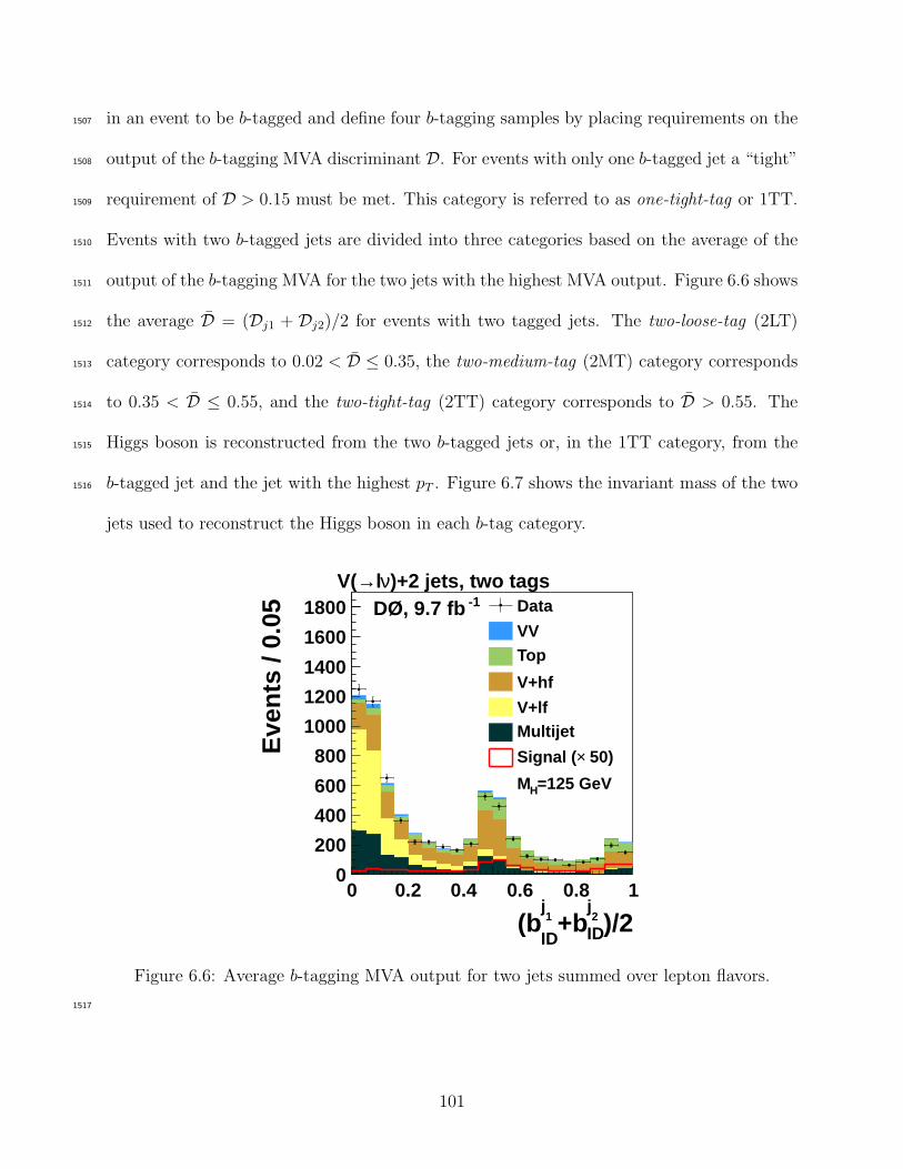
in an event to be b-tagged and define four b-tagging samples by placing requirements on the1507

output of the b-tagging MVA discriminant D. For events with only one b-tagged jet a “tight”1508

requirement of D > 0.15 must be met. This category is referred to as one-tight-tag or 1TT.1509

Events with two b-tagged jets are divided into three categories based on the average of the1510

output of the b-tagging MVA for the two jets with the highest MVA output. Figure 6.6 shows1511

the average D = (Dj1 + Dj2)/2 for events with two tagged jets. The two-loose-tag (2LT)1512

category corresponds to 0.02 < D ≤ 0.35, the two-medium-tag (2MT) category corresponds1513

to 0.35 < D ≤ 0.55, and the two-tight-tag (2TT) category corresponds to D > 0.55. The1514

Higgs boson is reconstructed from the two b-tagged jets or, in the 1TT category, from the1515

b-tagged jet and the jet with the highest pT . Figure 6.7 shows the invariant mass of the two1516

jets used to reconstruct the Higgs boson in each b-tag category.

)/22j

ID+b1j

ID(b

0 0.2 0.4 0.6 0.8 1

Eve

nts

/ 0.0

5

0

200

400

600

800

1000

1200

1400

1600

1800 -1DØ, 9.7 fb)+2 jets, two tagsνl→V(

Data

VVTop

V+hf

V+lfMultijet

50)×Signal (

=125 GeVHM

Figure 6.6: Average b-tagging MVA output for two jets summed over lepton flavors.

1517

101

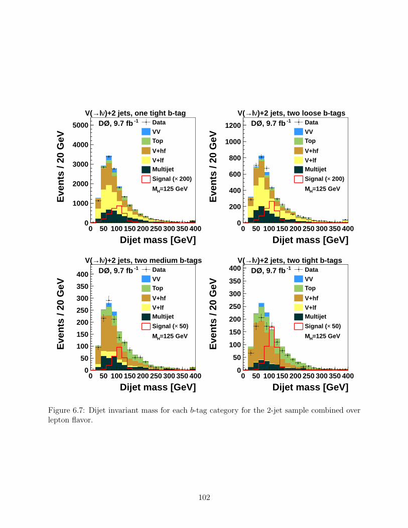
Dijet mass [GeV]0 50 100 150 200 250 300 350 400

Eve

nts

/ 20

GeV

0

1000

2000

3000

4000

5000 -1DØ, 9.7 fb

)+2 jets, one tight b-tagνl→V(Data

VVTop

V+hf

V+lfMultijet

200)×Signal (

=125 GeVHM

Dijet mass [GeV]0 50 100 150 200 250 300 350 400

Eve

nts

/ 20

GeV

0

200

400

600

800

1000

1200 -1DØ, 9.7 fb

)+2 jets, two loose b-tagsνl→V(Data

VVTop

V+hf

V+lfMultijet

200)×Signal (

=125 GeVHM

Dijet mass [GeV]0 50 100 150 200 250 300 350 400

Eve

nts

/ 20

GeV

0

50

100

150

200

250

300

350

400 -1DØ, 9.7 fb

)+2 jets, two medium b-tagsνl→V(Data

VVTop

V+hf

V+lfMultijet

50)×Signal (

=125 GeVHM

Dijet mass [GeV]0 50 100 150 200 250 300 350 400

Eve

nts

/ 20

GeV

0

50

100

150

200

250

300

350

400 -1DØ, 9.7 fb)+2 jets, two tight b-tagsνl→V(

Data

VVTop

V+hf

V+lfMultijet

50)×Signal (

=125 GeVHM

Figure 6.7: Dijet invariant mass for each b-tag category for the 2-jet sample combined overlepton flavor.

102

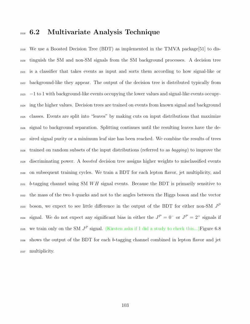
6.2 Multivariate Analysis Technique1518

We use a Boosted Decision Tree (BDT) as implemented in the TMVA package[51] to dis-1519

tinguish the SM and non-SM signals from the SM background processes. A decision tree1520

is a classifier that takes events as input and sorts them according to how signal-like or1521

background-like they appear. The output of the decision tree is distributed typically from1522

−1 to 1 with background-like events occupying the lower values and signal-like events occupy-1523

ing the higher values. Decision trees are trained on events from known signal and background1524

classes. Events are split into “leaves” by making cuts on input distributions that maximize1525

signal to background separation. Splitting continues until the resulting leaves have the de-1526

sired signal purity or a minimum leaf size has been reached. We combine the results of trees1527

trained on random subsets of the input distributions (referred to as bagging) to improve the1528

discriminating power. A boosted decision tree assigns higher weights to misclassified events1529

on subsequent training cycles. We train a BDT for each lepton flavor, jet multiplicity, and1530

b-tagging channel using SM WH signal events. Because the BDT is primarily sensitive to1531

the mass of the two b quarks and not to the angles between the Higgs boson and the vector1532

boson, we expect to see little difference in the output of the BDT for either non-SM JP1533

signal. We do not expect any significant bias in either the JP = 0− or JP = 2+ signals if1534

we train only on the SM JP signal. (Kirsten asks if I did a study to check this...)Figure 6.81535

shows the output of the BDT for each b-tagging channel combined in lepton flavor and jet1536

multiplicity.1537

103

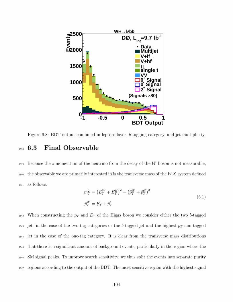
BDT Output-1 -0.5 0 0.5 1

Eve

nts

0

500

1000

1500

2000

2500 -1=9.7 fbint

DØ, L

80)×(Signals

DataMultijetV+lfV+hftt

single tVV

Signal+0 Signal-0 Signal+2

bbνl→WH

Figure 6.8: BDT output combined in lepton flavor, b-tagging category, and jet multiplicity.

6.3 Final Observable1538

Because the z momentum of the neutrino from the decay of the W boson is not measurable,1539

the observable we are primarily interested in is the transverse mass of the WX system defined1540

as follows.1541

m2T =

(EW

T + EHT

)2 −(~pW

T + ~pHT

)2

~pWT = ~6ET + ~pℓ

T

(6.1)

When constructing the pT and ET of the Higgs boson we consider either the two b-tagged1542

jets in the case of the two-tag categories or the b-tagged jet and the highest-pT non-tagged1543

jet in the case of the one-tag category. It is clear from the transverse mass distributions1544

that there is a significant amount of background events, particularly in the region where the1545

SM signal peaks. To improve search sensitivity, we thus split the events into separate purity1546

regions according to the output of the BDT. The most sensitive region with the highest signal1547

104

purity requires a BDT response value BDTout above 0.5. An intermediate region is defined1548

by 0 < BDTout ≤ 0.5. The lowest purity region are the events with BDTout ≤ 0. This region1549

provides insignificant sensitivity in the final result relative to the other two regions and we1550

do not include this region in the statistical analysis. The region with a BDT output above1551

0.5 is referred to as the “high-purity” (HP) channel and the region with 0 < BDTout ≤ 0.51552

is referred to as the “low-purity” (LP) channel. The final observables, split into high- and1553

low-purity regions, are given in Figs. 6.9 and 6.10. There are 32 channels that enter into1554

the statistical analysis described in Chapter 7 resulting from splitting the events by lepton1555

flavor, jet multiplicity, b-tagging category, and purity region.1556

105

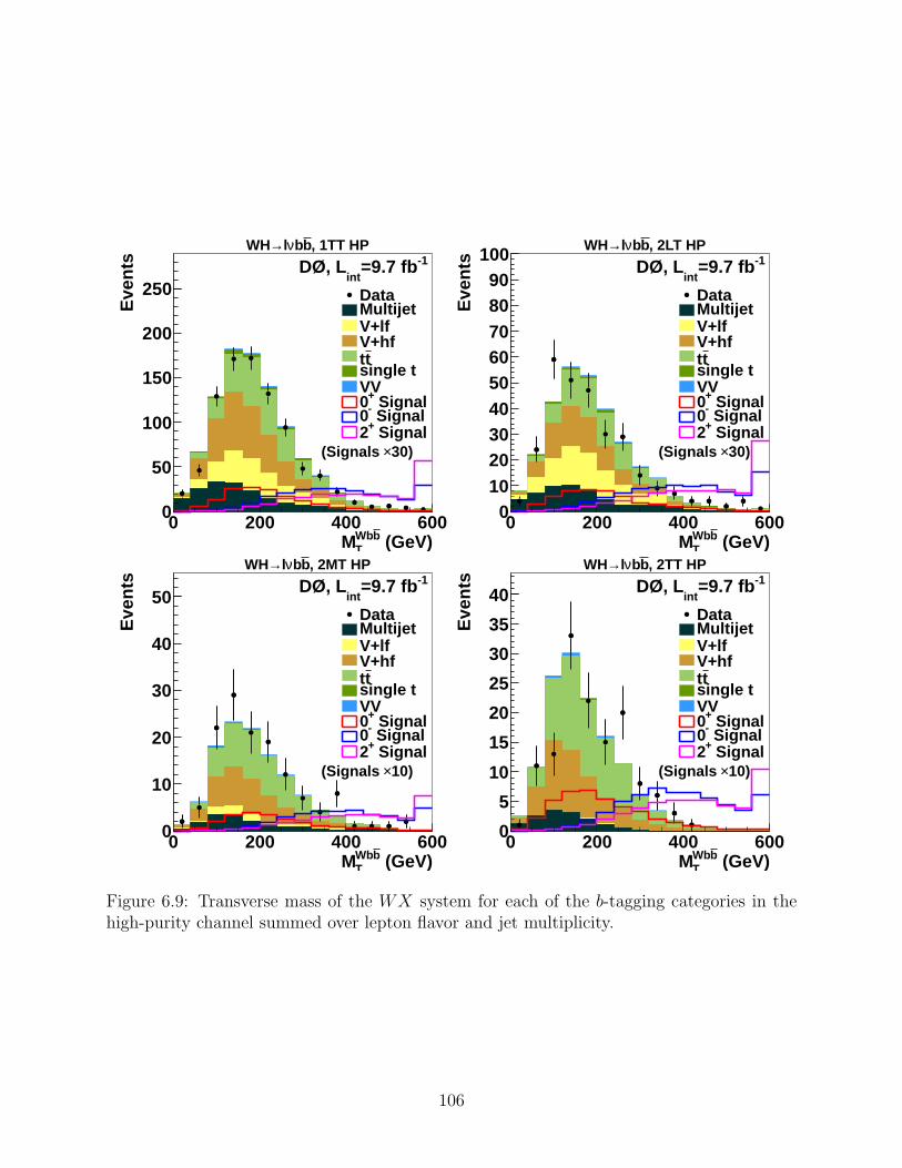
(GeV)bWbTM

0 200 400 600

Eve

nts

0

50

100

150

200

250

-1=9.7 fbint

DØ, L

30)×(Signals

DataMultijetV+lfV+hftt

single tVV

Signal+0 Signal-0 Signal+2

, 1TT HPbbνl→WH

(GeV)bWbTM

0 200 400 600

Eve

nts

0102030405060708090

100 -1=9.7 fbint

DØ, L

30)×(Signals

DataMultijetV+lfV+hftt

single tVV

Signal+0 Signal-0 Signal+2

, 2LT HPbbνl→WH

(GeV)bWbTM

0 200 400 600

Eve

nts

0

10

20

30

40

50-1=9.7 fb

intDØ, L

10)×(Signals

DataMultijetV+lfV+hftt

single tVV

Signal+0 Signal-0 Signal+2

, 2MT HPbbνl→WH

(GeV)bWbTM

0 200 400 600

Eve

nts

0

5

10

15

20

25

30

35

40-1=9.7 fb

intDØ, L

10)×(Signals

DataMultijetV+lfV+hftt

single tVV

Signal+0 Signal-0 Signal+2

, 2TT HPbbνl→WH

Figure 6.9: Transverse mass of the WX system for each of the b-tagging categories in thehigh-purity channel summed over lepton flavor and jet multiplicity.

106

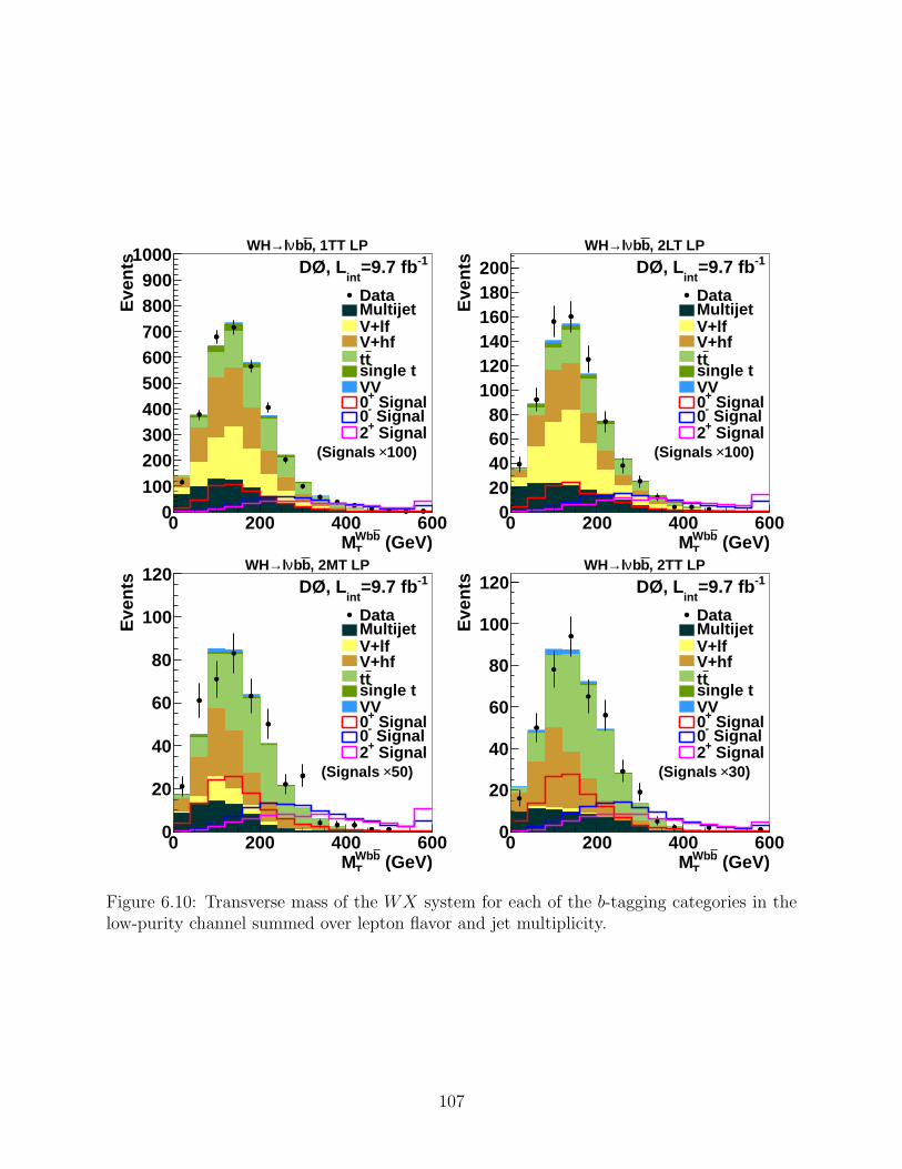
(GeV)bWbTM

0 200 400 600

Eve

nts

0100200300400500600700800900

1000 -1=9.7 fbint

DØ, L

100)×(Signals

DataMultijetV+lfV+hftt

single tVV

Signal+0 Signal-0 Signal+2

, 1TT LPbbνl→WH

(GeV)bWbTM

0 200 400 600

Eve

nts

020406080

100120140160180200 -1=9.7 fb

intDØ, L

100)×(Signals

DataMultijetV+lfV+hftt

single tVV

Signal+0 Signal-0 Signal+2

, 2LT LPbbνl→WH

(GeV)bWbTM

0 200 400 600

Eve

nts

0

20

40

60

80

100

120 -1=9.7 fbint

DØ, L

50)×(Signals

DataMultijetV+lfV+hftt

single tVV

Signal+0 Signal-0 Signal+2

, 2MT LPbbνl→WH

(GeV)bWbTM

0 200 400 600

Eve

nts

0

20

40

60

80

100

120 -1=9.7 fbint

DØ, L

30)×(Signals

DataMultijetV+lfV+hftt

single tVV

Signal+0 Signal-0 Signal+2

, 2TT LPbbνl→WH

Figure 6.10: Transverse mass of the WX system for each of the b-tagging categories in thelow-purity channel summed over lepton flavor and jet multiplicity.

107

Chapter 71557

Statistical Analysis1558

To answer the questions posed in Chapter 4 we must develop a framework to determine1559

the relative agreement of the data with our SM and non-SM Higgs boson hypotheses. The1560

probabilistic nature of particle interactions leads us to collect a large data sample to look for1561

rare processes and to accurately describe those which are more common. The most natural1562

framework is then a statistical one. Section 7.1 describes the hypothesis test and the test1563

statistic used in this analysis. The particular method we use for interpreting the results of1564

the hypothesis test, the CLs method, is described in Section 7.2. Finally, a description of1565

the systematic uncertainties present in this analysis is described in Section 7.3.1566

7.1 The Hypothesis Test1567

As described in Chapter 6, the result of a search for a new physics process is one or more1568

final variable distributions meant to distinguish between the new physics process and the1569

backgrounds. In this analysis the final variable is the transverse mass of the WH system. We1570

would like to define a hypothesis test based on this distribution that distinguishes between1571

having a Higgs boson with SM JP and one with exotic JP . The discriminating power of1572

the transverse mass comes from differences in the shape of the distribution for the SM and1573

non-SM JP signals. To incorporate the shape of the distribution in the statistical analysis1574

we perform a counting experiment in each bin of the final distribution. In the following, the1575

108

null hypothesis H0 refers to the standard model case: the final distribution will contain all1576

SM backgrounds and the SM Higgs boson signal with JP = 0+. Each test hypothesis H11577

will consider all SM backgrounds and the non-SM Higgs boson with one of the exotic JP1578

values, JP = 0− or JP = 2+.1579

The Neyman-Pearson lemma states that the likelihood ratio is the most powerful hy-1580

pothesis test when considering hypotheses which are fully-specified. The likelihood ratio is1581

defined as1582

Q =L(H1| data)

L(H0| data)(7.1)

where L(H| data) is the likelihood of hypothesis H given the data1. If we consider each bin1583

of the final variable distribution as a counting experiment with Poisson statistics then the1584

likelihood of hypothesis H given the distribution of the data is the product of individual1585

Poisson likelihood functions over all bins:1586

L(H| data) =

Nbins∏

i

(pi

di

)di

edi−pi (7.2)

where pi is the predicted number of events and di is the number of data events in the ith1587

bin. The predicted number of events will depend on the hypothesis considered. For the null1588

hypothesis the predicted number of events will be the sum of the SM Higgs boson signal1589

(sSMi ) and background (bi) predictions. For the test hypotheses pi will be the sum of the1590

non-SM Higgs boson signal (snSMi ) and background (bi) predictions. Because the natural1591

logarithm is monotonic, we can use the more convenient log-likelihood ratio LLR as our1592

test statistic without sacrificing the power of the likelihood ratio test. This changes the1593

1The likelihood is not a probability in the standard sense; it refers to events with known outcomes wherethe probability deals with future (unknown) events.

109

product in Eq. 7.2 to a simple summation. For our purposes we define the log-likelihood1594

ratio as LLR = −2 ln Q where the prefactor is chosen such that LLR → χ2 as the sample1595

size approaches infinity. Combining Eqs. 7.1 and 7.2 and performing some simple arithmetic1596

we obtain1597

LLR = 2

Nbins∑

i

(snSMi − sSM

i ) − 2

Nbins∑

i

di ln

(snSM

i + bi

sSMi + bi

)

. (7.3)

A test statistic provides an ordering rule with which sets of data can be determined as1598

belonging to one hypothesis over another. More positive values of the LLR defined in Eq. 7.31599

indicate that the observed data agree better with the null hypothesis while more negative1600

values indicate better agreement with the test hypothesis. However, without context, the1601

LLR value calculated from the data is essentially meaningless. We can calculate the expected1602

values of the LLR by substituting the di in Eq. 7.3 by sSMi + bi or snSM

i + bi but in order1603

to gauge the importance of any deviations we need to know the distribution of LLR values1604

for each hypothesis. This is done by simulating the outcomes of repeated experiments or1605

pseudo-experiments. Again, to retain the information stored in the shape of the final variable1606

distribution we proceed with a per-bin calculation. In each bin we assume that the data was1607

drawn randomly from a Poisson parent distribution with a mean equal to the predicted1608

number of events pi. We then generate pseudo-data by randomly drawing a value from this1609

Poisson parent distribution. We iterate over the total number of bins and the value of the1610

LLR is calculated. This process is repeated many times to create two LLR distributions:1611

one assuming the null hypothesis is true and one assuming the test hypothesis is true.1612

A complication arises from the fact that the hypotheses we consider are not fully-specified.1613

The background and signal predictions depend on many parameters such as the integrated1614

luminosity, selection efficiencies, and cross sections. These parameters are not of primary1615

110

interest themselves but must be taken into account because of their associated uncertainties.1616

We refer to them as ‘nuisance parameters’. One method of dealing with these nuisance1617

parameters is to assume they are Gaussian-distributed with a mean equal to the best estimate1618

of the nuisance parameter θ0j and a standard deviation σj equal to its uncertainty. By varying1619

the values of the nuisance parameters for each pseudo-experiment we can incorporate the1620

effect their uncertainties have on the results. Changing the values of the nuisance parameters1621

will produce a change in the number of predicted events. For an individual bin, the number1622

of predicted events pi can be written in terms of the nominal prediction pi and a deviation1623

from the best estimate for each nuisance parameter Rj = (θj − θ0j )/σj as1624

pi = pi +

Npar∑

j

Rjδj (7.4)

where δj is the fractional change in the number of events for the nuisance parameter j and1625

the sum is over the number of nuisance parameters. This Gaussian represents our prior1626

knowledge of the values of the nuisance parameters. Before generating a set of pseudo-data1627

we vary the values of the nuisance parameters by randomly sampling their Gaussian priors1628

and adjust the predicted number of events accordingly. Next we generate the pseudo-data1629

by randomly drawing a value from the Poisson parent distribution with a mean equal to the1630

(adjusted) predicted number of events. The likelihood function in Eq. 7.2 is modified by the1631

introduction of a Gaussian likelihood term. The likelihood function is thus a product of a1632

Poisson likelihood LP and a Gaussian likelihood LG:1633

L(H| data) = LP × LG

=

Nbins∏

i

(pi

di

)di

edi−pi ×Npar∏

j

e−R2j/2

(7.5)

111

where the di are the (pseudo-)data and the products go over the number of bins Nbins and1634

the number of nuisance parameters Npar. Note that the predicted number of events pi is1635

now a function of the deviation Rj. The second term reflects the deviations of the nuisance1636

parameters as a function of their prior which takes into account the relative agreement with1637

the prior estimate.1638

The uncertainties on the nuisance parameters can be large, sometimes as large as ≈ 30% of1639

the nominal value. Allowing the nuisance parameters to vary according to their uncertainties1640

therefore has the unfortunate effect of diluting the power of the statistical test by broadening1641

the width of the LLR distribution for each hypothesis. We mitigate this effect by performing1642

a “best-fit” to the data by maximizing the likelihood function in Eq. 7.5 over the Rj. The1643

Gaussian likelihood term LG serves as a penalty term for the maximization. The effect of the1644

prior is to constrain the fit within the uncertainty of the best estimate. Two fits, one for each1645

hypothesis, are performed for each pseudo-experiment and the data. The final test statistic1646

is the log-likelihood ratio of the maximized likelihood functions and can be summarized as1647

the following:1648

LLR = −2 ln

(

L(H1| data, θ)

L(H0| data,ˆθ)

)

(7.6)

where the θ (ˆθ) represent the values of the nuisance parameters that maximize the likelihood1649

for the H1 (H0) hypothesis.1650

In the preceding we have implicitly assumed only one source of events but in reality1651

there are often several sources of backgrounds and signals that must enter into the predicted1652

number of events. This can be accomplished with additional summations in Eq. 7.4. Multiple1653

channels can be incorporated in a similar matter. They can either represent subdivisions1654

in the data or a complete set of final variable histograms with their associated predicted1655

112

number of events and nuisance parameters.1656

7.2 CLs Method1657

After obtaining the LLR distributions we use them to interpret our observed data. Figure 7.11658

illustrates example LLR distributions for the null and test hypotheses and well as an example1659

observed value. Two important p-values can be calculated from the LLR distributions and1660

the observed data. A p-value is defined as the probability of obtaining a result at least as or1661

more extreme than what was observed, assuming the hypothesis under consideration is true.1662

If we consider that the test hypothesis is true more extreme LLR values than the observed1663

LLR value lie towards the null hypothesis distribution. The p-value for the test hypothesis1664

ptest is therefore the integral of the H1 LLR distribution to the right of the observed value1665

LLRobs as indicated by the red region in Fig. 7.1. On the other hand if we assume that the1666

null hypothesis is true more extreme values lie towards the test hypothesis distribution and1667

the p-value for the H0 hypothesis pnull is the integral of the H0 LLR distribution to the left1668

of LLRobs. This is illustrated by the blue region in Fig. 7.1. We select a significance level1669

α of 5% against which we will test our result. If the resulting p-value is less than or equal1670

to α we reject the hypothesis at the 1 − α confidence level (CL). A strict frequentist inter-1671

pretation would only consider ptest when determining whether to reject the test hypothesis.1672

However, as demonstrated in the previous section, the null and test hypotheses depend on1673

many parameters which can result in poor modeling of either hypothesis. To provide some1674

protection against this poor modeling we use the CLs method[52, 53, 54]. We define a new1675

quantity CLs:1676

CLs = 1 − ptest

1 − pnull

(7.7)

113

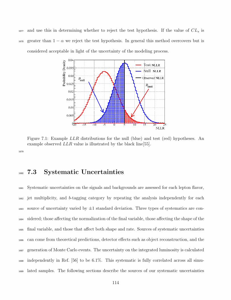
and use this in determining whether to reject the test hypothesis. If the value of CLs is1677

greater than 1 − α we reject the test hypothesis. In general this method overcovers but is1678

considered acceptable in light of the uncertainty of the modeling process.

Figure 7.1: Example LLR distributions for the null (blue) and test (red) hypotheses. Anexample observed LLR value is illustrated by the black line[55].

1679

7.3 Systematic Uncertainties1680

Systematic uncertainties on the signals and backgrounds are assessed for each lepton flavor,1681

jet multiplicity, and b-tagging category by repeating the analysis independently for each1682

source of uncertainty varied by ±1 standard deviation. Three types of systematics are con-1683

sidered; those affecting the normalization of the final variable, those affecting the shape of the1684

final variable, and those that affect both shape and rate. Sources of systematic uncertainties1685

can come from theoretical predictions, detector effects such as object reconstruction, and the1686

generation of Monte Carlo events. The uncertainty on the integrated luminosity is calculated1687

independently in Ref. [56] to be 6.1%. This systematic is fully correlated across all simu-1688

lated samples. The following sections describe the sources of our systematic uncertainties1689

114

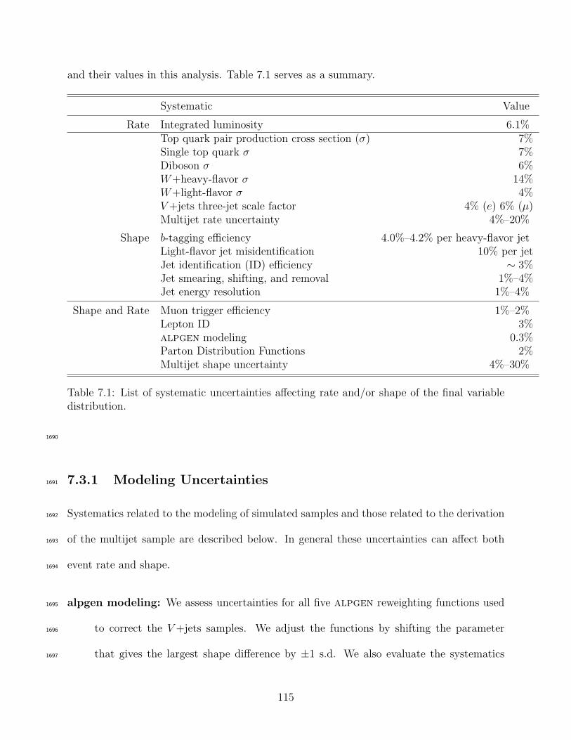
and their values in this analysis. Table 7.1 serves as a summary.

Systematic Value

Rate Integrated luminosity 6.1%Top quark pair production cross section (σ) 7%Single top quark σ 7%Diboson σ 6%W+heavy-flavor σ 14%W+light-flavor σ 4%V +jets three-jet scale factor 4% (e) 6% (µ)Multijet rate uncertainty 4%–20%

Shape b-tagging efficiency 4.0%–4.2% per heavy-flavor jetLight-flavor jet misidentification 10% per jetJet identification (ID) efficiency ∼ 3%Jet smearing, shifting, and removal 1%–4%Jet energy resolution 1%–4%

Shape and Rate Muon trigger efficiency 1%–2%Lepton ID 3%alpgen modeling 0.3%Parton Distribution Functions 2%Multijet shape uncertainty 4%–30%

Table 7.1: List of systematic uncertainties affecting rate and/or shape of the final variabledistribution.

1690

7.3.1 Modeling Uncertainties1691

Systematics related to the modeling of simulated samples and those related to the derivation1692

of the multijet sample are described below. In general these uncertainties can affect both1693

event rate and shape.1694

alpgen modeling: We assess uncertainties for all five alpgen reweighting functions used1695

to correct the V +jets samples. We adjust the functions by shifting the parameter1696

that gives the largest shape difference by ±1 s.d. We also evaluate the systematics1697

115

related to the jet-to-parton matching scheme and the underlying event modeling used1698

by alpgen.1699

V +jets three-jet scale factors: When we simultaneously normalize the V +jets and mul-1700

tijet samples by performing a fit to the data we find that the scaling factors we apply1701

to the 3-jet V +jets sample differ significantly from unity. We therefore apply an addi-1702

tional uncertainty on the 3-jet V +jets sample that is uncorrelated with lepton flavor.1703

We also apply a normalization uncertainty on V +jets events that is anticorrelated with1704

the multijet rate systematic.1705

Multijet rate: We assign uncertainties on the multijet event rate of 15% in the electron1706

channel and 20% in the muon channel. This systematic is uncorrelated across lepton1707

flavor, jet multiplicity, and b-tagging category.1708

Multijet shape: To determine the uncertainty on the shape of our multijet estimate we1709

relax the triangle cut introduced in Section 6.1 to mWT > 30 − 0.56ET and repeat the1710

analysis. The positive and negative variations are taken to be symmetric.1711

7.3.2 Theoretical Uncertainties1712

Theoretical systematic effects can enter into the analysis from several sources such as pre-1713

dicted cross sections and PDF sets. These can affect both the event rate and shape of the1714

final distribution. We therefore assess uncertainties associated with these items.1715

Cross section predictions: For single top quark production and top quark pair produc-1716

tion this uncertainty is 7%[57, 58] The uncertainty on the diboson production cross1717

section is 6%[59]. The uncertainties on W+hf and W+lf production are 14% and 4%,1718

respectively. The uncertainties on W+hf are estimated with mcfm[60, 61].1719

116

PDF sets: Sets of parton distribution functions are calculated from theory and experimen-1720

tal results. The choice of PDF set used in Monte Carlo event generation affects the1721

signal and background rates. We assign an uncertainty of 2% to account for this.1722

7.3.3 Jet Systematics1723

There are several systematics associated with the presence of jets in the final state. These1724

uncertainties come from detector effects, object reconstruction, and b-tagging algorithms.1725

Jet energy scale: The energy we measure for a jet is corrected to account for detector1726

effects such as uranium decay in the calorimeter, electronics noise, residual energy from1727

previous collisions, and inactive areas of the detector. This correction is referred to the1728

Jet Energy Scale (JES) correction and it is applied to both the data and MC events.1729

The uncertainty on the JES correction is assessed by shifting the JES parameters up1730

and down by 1 s.d.1731

Jet smearing, shifting, and removal: Jets produced in MC events must be smeared and1732

shifted in energy to match the characteristics of jets in data. We apply the Jet Smear-1733

ing Shifting and Removal (JSSR) correction to jets in MC. The uncertainty on this1734

correction is found by shifting the parameters by ±1 s.d.1735

Jet identification: We assign a 2% uncertainty on the jet identification efficiency.1736

b quark identification: The uncertainty on the b-tagging efficiency is determined by vary-1737

ing the tagging rate functions up and down 1 s.d. in samples containing heavy-flavor1738

jets. The uncertainty on the light-flavor misidentification rate is determined by varying1739

the light-flavor tag rates by ±1 s.d. in samples with no heavy-flavor jets.1740

117

7.3.4 Lepton Systematics1741

There are several systematics associated with the presence of leptons in the final state. These1742

systematics can affect both event rate and shape.1743

Electron identification: We assign an uncertainty of 3% on the electron identification1744

efficiency. Included in this uncertainty is the uncertainty associated with the EM1745

trigger.1746

Muon identification: We also assign an uncertainty of 3% on the muon identification1747

efficiency.1748

Muon trigger: The alpgen reweightings are calculated using the TµOR trigger suite and1749

applied to both events with electrons and events with muons. Additional reweightings1750

are applied to the muon channel which are calculated from events selected with Tincl. To1751

account for the difference between the alpgen reweightings as applied to the electron1752

events and muons events we apply an uncertainty on the muon trigger. It is calculated1753

as the difference between applying the nominal trigger correction and applying a trigger1754

correction derived using the alpgen reweightings calculated using the TµOR trigger1755

suite.1756

118

Chapter 81757

Results and Interpretations1758

The statistical method outlined in Chapter 7 can be used to investigate several questions1759

related to the spin and parity of the particle discovered at the LHC. Is the new particle1760

really the SM Higgs boson? At what level can we exclude other non-SM JP assignments? Is1761

the particle an admixture of different JP states? Under the assumption that it is, would it1762

be possible to rule out any fraction of non-SM JP content? To answer these questions, I’ve1763

divided the results into two cases:1764

1. The new particle exists as a pure JP state1765

Of primary interest is whether or not the new particle is the SM Higgs boson. Since1766

the Tevatron cannot measure the spin and parity of the particle directly we can only1767

exclude models with exotic JP . Whether or not we exclude these models depends1768

in part on the total predicted cross section for the process. Unfortunately, the total1769

predicted cross section for the JP = 0− and JP = 2+ states is incalculable and the1770

exclusion will depend on an assumed signal cross section. One very reasonable starting1771

point would be the observed rate in data.1772

2. The new particle exists as an admixture of JP states1773

Another important possibility to exclude is whether the discovered particle is a pure1774

JP state or an admixture of JP states. Excluding this possibility in its entirety requires1775

excluding all possible fractions of non-SM signals. Any exclusions in this case will again1776

119

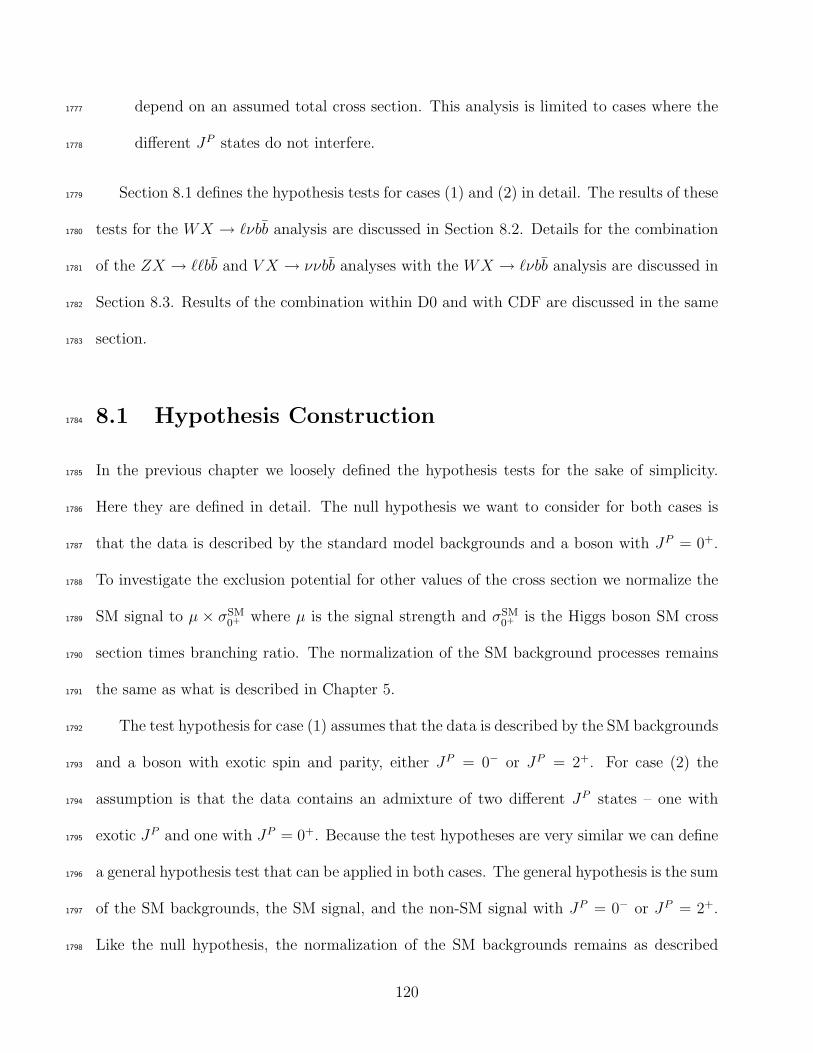
depend on an assumed total cross section. This analysis is limited to cases where the1777

different JP states do not interfere.1778

Section 8.1 defines the hypothesis tests for cases (1) and (2) in detail. The results of these1779

tests for the WX → ℓνbb analysis are discussed in Section 8.2. Details for the combination1780

of the ZX → ℓℓbb and V X → ννbb analyses with the WX → ℓνbb analysis are discussed in1781

Section 8.3. Results of the combination within D0 and with CDF are discussed in the same1782

section.1783

8.1 Hypothesis Construction1784

In the previous chapter we loosely defined the hypothesis tests for the sake of simplicity.1785

Here they are defined in detail. The null hypothesis we want to consider for both cases is1786

that the data is described by the standard model backgrounds and a boson with JP = 0+.1787

To investigate the exclusion potential for other values of the cross section we normalize the1788

SM signal to µ × σSM0+ where µ is the signal strength and σSM

0+ is the Higgs boson SM cross1789

section times branching ratio. The normalization of the SM background processes remains1790

the same as what is described in Chapter 5.1791

The test hypothesis for case (1) assumes that the data is described by the SM backgrounds1792

and a boson with exotic spin and parity, either JP = 0− or JP = 2+. For case (2) the1793

assumption is that the data contains an admixture of two different JP states – one with1794

exotic JP and one with JP = 0+. Because the test hypotheses are very similar we can define1795

a general hypothesis test that can be applied in both cases. The general hypothesis is the sum1796

of the SM backgrounds, the SM signal, and the non-SM signal with JP = 0− or JP = 2+.1797

Like the null hypothesis, the normalization of the SM backgrounds remains as described1798

120

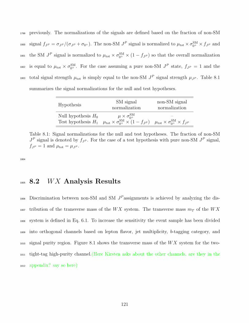
previously. The normalizations of the signals are defined based on the fraction of non-SM1799

signal fJP = σJP /(σJP + σ0+). The non-SM JP signal is normalized to µtot × σSM0+ × fJP and1800

the SM JP signal is normalized to µtot × σSM0+ × (1 − fJP ) so that the overall normalization1801

is equal to µtot × σSM0+ . For the case assuming a pure non-SM JP state, fJP = 1 and the1802

total signal strength µtot is simply equal to the non-SM JP signal strength µJP . Table 8.11803

summarizes the signal normalizations for the null and test hypotheses.

HypothesisSM signal non-SM signal

normalization normalization

Null hypothesis H0 µ × σSM0+ –

Test hypothesis H1 µtot × σSM0+ × (1 − fJP ) µtot × σSM

0+ × fJP

Table 8.1: Signal normalizations for the null and test hypotheses. The fraction of non-SMJP signal is denoted by fJP . For the case of a test hypothesis with pure non-SM JP signal,fJP = 1 and µtot = µJP .

1804

8.2 WX Analysis Results1805

Discrimination between non-SM and SM JP assignments is achieved by analyzing the dis-1806

tribution of the transverse mass of the WX system. The transverse mass mT of the WX1807

system is defined in Eq. 6.1. To increase the sensitivity the event sample has been divided1808

into orthogonal channels based on lepton flavor, jet multiplicity, b-tagging category, and1809

signal purity region. Figure 8.1 shows the transverse mass of the WX system for the two-1810

tight-tag high-purity channel.(Here Kirsten asks about the other channels, are they in the1811

appendix? say so here)1812

121

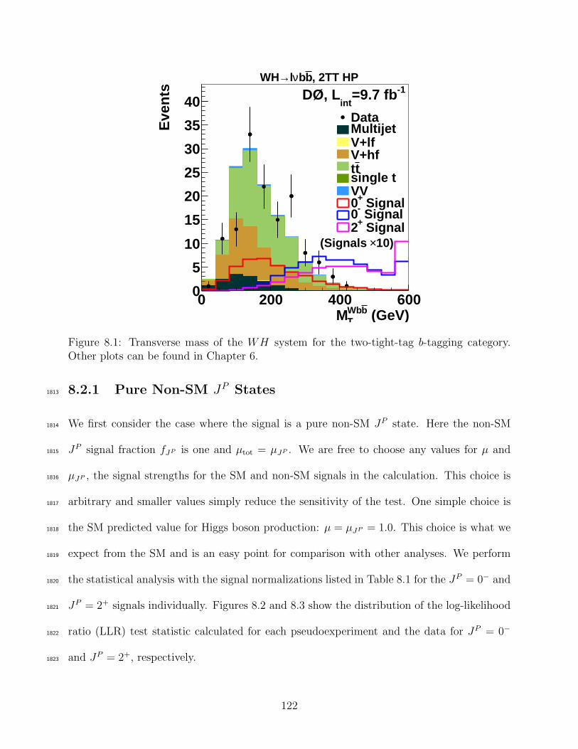
(GeV)bWbTM

0 200 400 600

Eve

nts

0

5

10

15

20

25

30

35

40-1=9.7 fb

intDØ, L

10)×(Signals

DataMultijetV+lfV+hftt

single tVV

Signal+0 Signal-0 Signal+2

, 2TT HPbbνl→WH

Figure 8.1: Transverse mass of the WH system for the two-tight-tag b-tagging category.Other plots can be found in Chapter 6.

8.2.1 Pure Non-SM JP States1813

We first consider the case where the signal is a pure non-SM JP state. Here the non-SM1814

JP signal fraction fJP is one and µtot = µJP . We are free to choose any values for µ and1815

µJP , the signal strengths for the SM and non-SM signals in the calculation. This choice is1816

arbitrary and smaller values simply reduce the sensitivity of the test. One simple choice is1817

the SM predicted value for Higgs boson production: µ = µJP = 1.0. This choice is what we1818

expect from the SM and is an easy point for comparison with other analyses. We perform1819

the statistical analysis with the signal normalizations listed in Table 8.1 for the JP = 0− and1820

JP = 2+ signals individually. Figures 8.2 and 8.3 show the distribution of the log-likelihood1821

ratio (LLR) test statistic calculated for each pseudoexperiment and the data for JP = 0−1822

and JP = 2+, respectively.1823

122

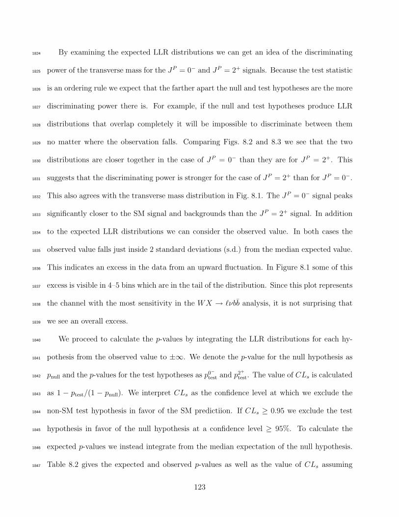
By examining the expected LLR distributions we can get an idea of the discriminating1824

power of the transverse mass for the JP = 0− and JP = 2+ signals. Because the test statistic1825

is an ordering rule we expect that the farther apart the null and test hypotheses are the more1826

discriminating power there is. For example, if the null and test hypotheses produce LLR1827

distributions that overlap completely it will be impossible to discriminate between them1828

no matter where the observation falls. Comparing Figs. 8.2 and 8.3 we see that the two1829

distributions are closer together in the case of JP = 0− than they are for JP = 2+. This1830

suggests that the discriminating power is stronger for the case of JP = 2+ than for JP = 0−.1831

This also agrees with the transverse mass distribution in Fig. 8.1. The JP = 0− signal peaks1832

significantly closer to the SM signal and backgrounds than the JP = 2+ signal. In addition1833

to the expected LLR distributions we can consider the observed value. In both cases the1834

observed value falls just inside 2 standard deviations (s.d.) from the median expected value.1835

This indicates an excess in the data from an upward fluctuation. In Figure 8.1 some of this1836

excess is visible in 4–5 bins which are in the tail of the distribution. Since this plot represents1837

the channel with the most sensitivity in the WX → ℓνbb analysis, it is not surprising that1838

we see an overall excess.1839

We proceed to calculate the p-values by integrating the LLR distributions for each hy-1840

pothesis from the observed value to ±∞. We denote the p-value for the null hypothesis as1841

pnull and the p-values for the test hypotheses as p0−

test and p2+

test. The value of CLs is calculated1842

as 1 − ptest/(1 − pnull). We interpret CLs as the confidence level at which we exclude the1843

non-SM test hypothesis in favor of the SM predictiion. If CLs ≥ 0.95 we exclude the test1844

hypothesis in favor of the null hypothesis at a confidence level ≥ 95%. To calculate the1845

expected p-values we instead integrate from the median expectation of the null hypothesis.1846

Table 8.2 gives the expected and observed p-values as well as the value of CLs assuming1847

123

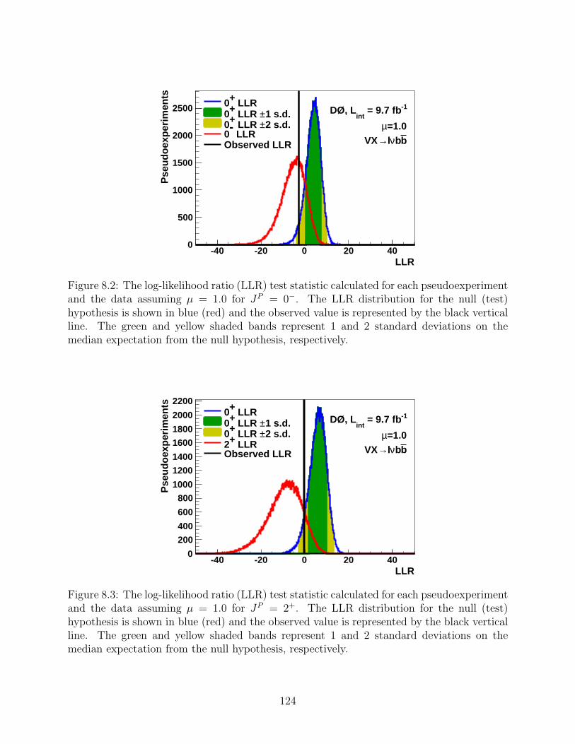
LLR-40 -20 0 20 40

Pse

udoe

xper

imen

ts

0

500

1000

1500

2000

2500 LLR+01 s.d.± LLR +02 s.d.± LLR +0

LLR-

0Observed LLR

-1 = 9.7 fbint

DØ, L

=1.0µbbνl→VX

Figure 8.2: The log-likelihood ratio (LLR) test statistic calculated for each pseudoexperimentand the data assuming µ = 1.0 for JP = 0−. The LLR distribution for the null (test)hypothesis is shown in blue (red) and the observed value is represented by the black verticalline. The green and yellow shaded bands represent 1 and 2 standard deviations on themedian expectation from the null hypothesis, respectively.

LLR-40 -20 0 20 40

Pse

udoe

xper

imen

ts

0

200

400

600

800

1000

1200

1400

1600

1800

2000

2200 LLR+0

1 s.d.± LLR +02 s.d.± LLR +0

LLR+2Observed LLR

-1 = 9.7 fbint

DØ, L

=1.0µbbνl→VX

Figure 8.3: The log-likelihood ratio (LLR) test statistic calculated for each pseudoexperimentand the data assuming µ = 1.0 for JP = 2+. The LLR distribution for the null (test)hypothesis is shown in blue (red) and the observed value is represented by the black verticalline. The green and yellow shaded bands represent 1 and 2 standard deviations on themedian expectation from the null hypothesis, respectively.

124

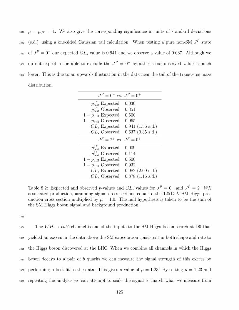
µ = µJP = 1. We also give the corresponding significance in units of standard deviations1848

(s.d.) using a one-sided Gaussian tail calculation. When testing a pure non-SM JP state1849

of JP = 0− our expected CLs value is 0.941 and we observe a value of 0.637. Although we1850

do not expect to be able to exclude the JP = 0− hypothesis our observed value is much1851

lower. This is due to an upwards fluctuation in the data near the tail of the transverse mass1852

distribution.

JP = 0− vs. JP = 0+

p0−

test Expected 0.030

p0−

test Observed 0.3511 − pnull Expected 0.5001 − pnull Observed 0.965

CLs Expected 0.941 (1.56 s.d.)CLs Observed 0.637 (0.35 s.d.)

JP = 2+ vs. JP = 0+

p2+

test Expected 0.009

p2+

test Observed 0.1141 − pnull Expected 0.5001 − pnull Observed 0.932

CLs Expected 0.982 (2.09 s.d.)CLs Observed 0.878 (1.16 s.d.)

Table 8.2: Expected and observed p-values and CLs values for JP = 0− and JP = 2+ WX

associated production, assuming signal cross sections equal to the 125 GeV SM Higgs pro-duction cross section multiplied by µ = 1.0. The null hypothesis is taken to be the sum ofthe SM Higgs boson signal and background production.

1853

The WH → ℓνbb channel is one of the inputs to the SM Higgs boson search at D0 that1854

yielded an excess in the data above the SM expectation consistent in both shape and rate to1855

the Higgs boson discovered at the LHC. When we combine all channels in which the Higgs1856

boson decays to a pair of b quarks we can measure the signal strength of this excess by1857

performing a best fit to the data. This gives a value of µ = 1.23. By setting µ = 1.23 and1858

repeating the analysis we can attempt to scale the signal to match what we measure from1859

125

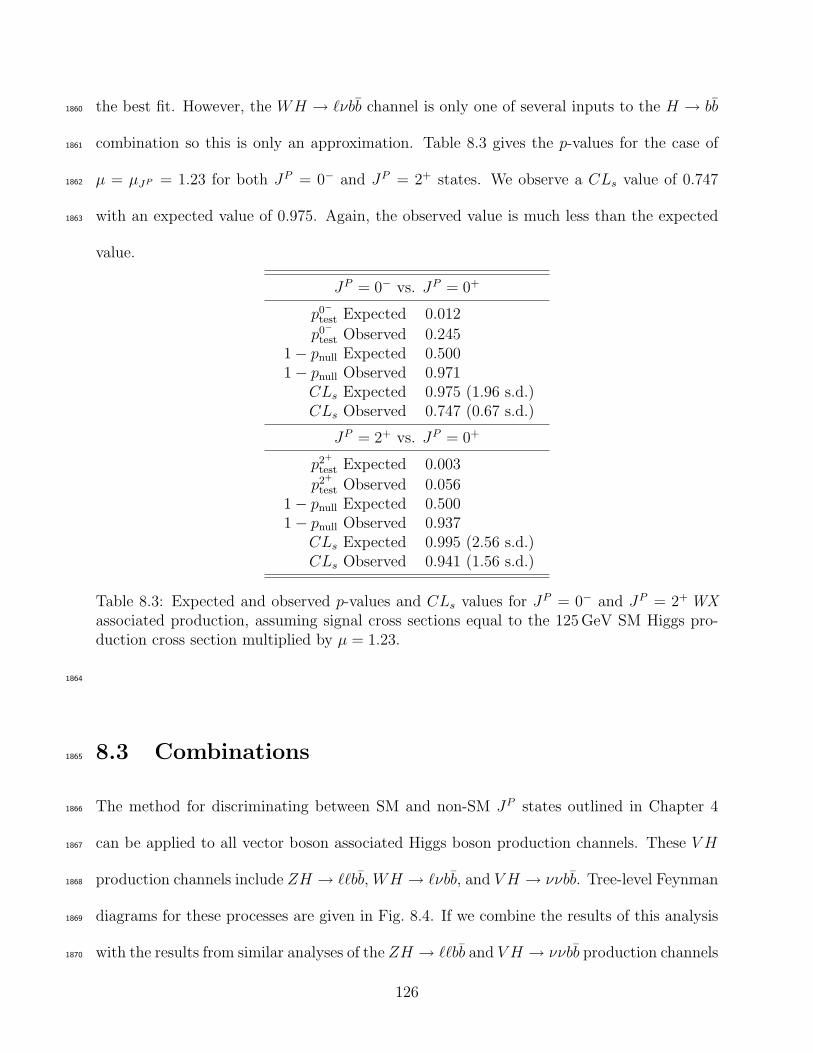
the best fit. However, the WH → ℓνbb channel is only one of several inputs to the H → bb1860

combination so this is only an approximation. Table 8.3 gives the p-values for the case of1861

µ = µJP = 1.23 for both JP = 0− and JP = 2+ states. We observe a CLs value of 0.7471862

with an expected value of 0.975. Again, the observed value is much less than the expected1863

value.

JP = 0− vs. JP = 0+

p0−

test Expected 0.012

p0−

test Observed 0.2451 − pnull Expected 0.5001 − pnull Observed 0.971

CLs Expected 0.975 (1.96 s.d.)CLs Observed 0.747 (0.67 s.d.)

JP = 2+ vs. JP = 0+

p2+

test Expected 0.003

p2+

test Observed 0.0561 − pnull Expected 0.5001 − pnull Observed 0.937

CLs Expected 0.995 (2.56 s.d.)CLs Observed 0.941 (1.56 s.d.)

Table 8.3: Expected and observed p-values and CLs values for JP = 0− and JP = 2+ WX

associated production, assuming signal cross sections equal to the 125 GeV SM Higgs pro-duction cross section multiplied by µ = 1.23.

1864

8.3 Combinations1865

The method for discriminating between SM and non-SM JP states outlined in Chapter 41866

can be applied to all vector boson associated Higgs boson production channels. These V H1867

production channels include ZH → ℓℓbb, WH → ℓνbb, and V H → ννbb. Tree-level Feynman1868

diagrams for these processes are given in Fig. 8.4. If we combine the results of this analysis1869

with the results from similar analyses of the ZH → ℓℓbb and V H → ννbb production channels1870

126

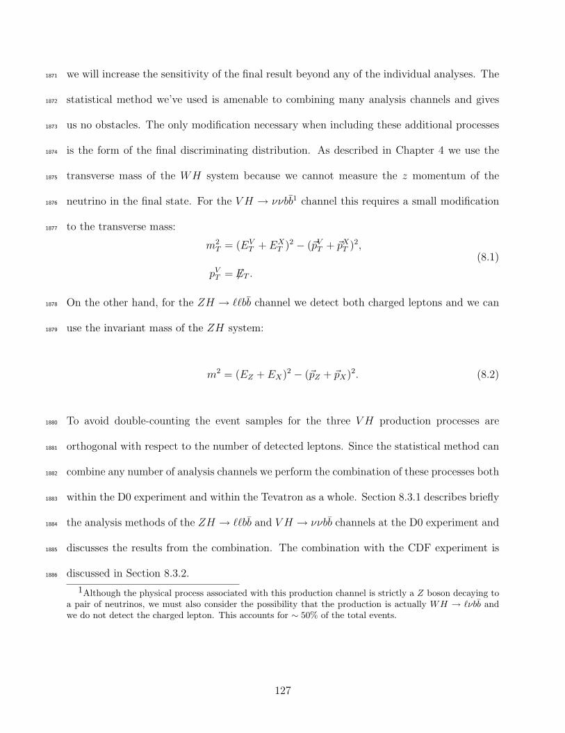
we will increase the sensitivity of the final result beyond any of the individual analyses. The1871

statistical method we’ve used is amenable to combining many analysis channels and gives1872

us no obstacles. The only modification necessary when including these additional processes1873

is the form of the final discriminating distribution. As described in Chapter 4 we use the1874

transverse mass of the WH system because we cannot measure the z momentum of the1875

neutrino in the final state. For the V H → ννbb1 channel this requires a small modification1876

to the transverse mass:1877

m2T = (EV

T + EXT )2 − (~pV

T + ~pXT )2,

pVT = 6ET .

(8.1)

On the other hand, for the ZH → ℓℓbb channel we detect both charged leptons and we can1878

use the invariant mass of the ZH system:1879

m2 = (EZ + EX)2 − (~pZ + ~pX)2. (8.2)

To avoid double-counting the event samples for the three V H production processes are1880

orthogonal with respect to the number of detected leptons. Since the statistical method can1881

combine any number of analysis channels we perform the combination of these processes both1882

within the D0 experiment and within the Tevatron as a whole. Section 8.3.1 describes briefly1883

the analysis methods of the ZH → ℓℓbb and V H → ννbb channels at the D0 experiment and1884

discusses the results from the combination. The combination with the CDF experiment is1885

discussed in Section 8.3.2.1886

1Although the physical process associated with this production channel is strictly a Z boson decaying toa pair of neutrinos, we must also consider the possibility that the production is actually WH → ℓνbb andwe do not detect the charged lepton. This accounts for ∼ 50% of the total events.

127

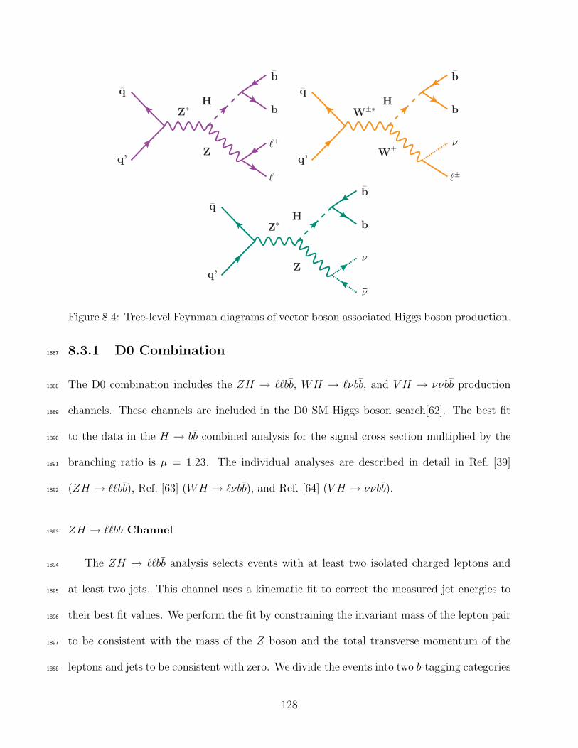
Hq

Zq’

Z∗

b

b

ℓ+

ℓ−

Hq

W±

q’

W±∗

b

b

ν

ℓ±

Hq

Zq’

Z∗

b

b

ν

ν

Figure 8.4: Tree-level Feynman diagrams of vector boson associated Higgs boson production.

8.3.1 D0 Combination1887

The D0 combination includes the ZH → ℓℓbb, WH → ℓνbb, and V H → ννbb production1888

channels. These channels are included in the D0 SM Higgs boson search[62]. The best fit1889

to the data in the H → bb combined analysis for the signal cross section multiplied by the1890

branching ratio is µ = 1.23. The individual analyses are described in detail in Ref. [39]1891

(ZH → ℓℓbb), Ref. [63] (WH → ℓνbb), and Ref. [64] (V H → ννbb).1892

ZH → ℓℓbb Channel1893

The ZH → ℓℓbb analysis selects events with at least two isolated charged leptons and1894

at least two jets. This channel uses a kinematic fit to correct the measured jet energies to1895

their best fit values. We perform the fit by constraining the invariant mass of the lepton pair1896

to be consistent with the mass of the Z boson and the total transverse momentum of the1897

leptons and jets to be consistent with zero. We divide the events into two b-tagging categories1898

128

depending on the number of b quark jets tagged in the event: a “single-tag” category (ST)1899

and a “double-tag” category (DT). The SM Higgs boson search[39] uses Random Forest1900

discriminants to produce the final distributions for the statistical analysis.1901

One of these Random Forests provides discrimination against top quark pair production1902

and divides the events into tt-enriched and tt-depleted regions. For the spin and parity1903

analysis only the events in the tt-depleted region are considered2. The invariant mass is1904

constructed from the two leptons and either the two b-tagged jets (DT) or one tagged jet1905

and the untagged jet with the highest pT . To improve the discrimination between the non-1906

SM signals and the backgrounds we use the invariant mass of the dijet system Mjj to select1907

two regions with different purity regions. The invariant mass of the dijet system is shown1908

in Fig. 8.5. Events with 100 ≤ Mjj ≤ 150 GeV comprise the “high-purity” region while1909

the remaining events are in the “low-purity” region. Figure 8.6 shows the invariant mass1910

distribution of the ZH system for the DT b-tagging category in the high-purity region.1911

Additional distributions are given in Appendix B.1912

V H → ννbb Channel1913

The SM Higgs boson search in the V H → ννbb channel selects events with a large 6ET and1914

exactly two jets. This channel is sensitive to WH associated production when the charged1915

lepton is not detected. The jets are classified into two b-tagging categories depending on1916

the sum of the scores provided by the tagging algorithm. These categories are referred to as1917

“medium” (MT) and “tight” (TT). We use a dedicated boosted decision tree to provide some1918

rejection of the multijet background. The SM Higgs boson search uses a boosted decision1919

tree discriminant as the final distribution in the statistical analysis.1920

2This region contains roughly 94% of the signal.

129

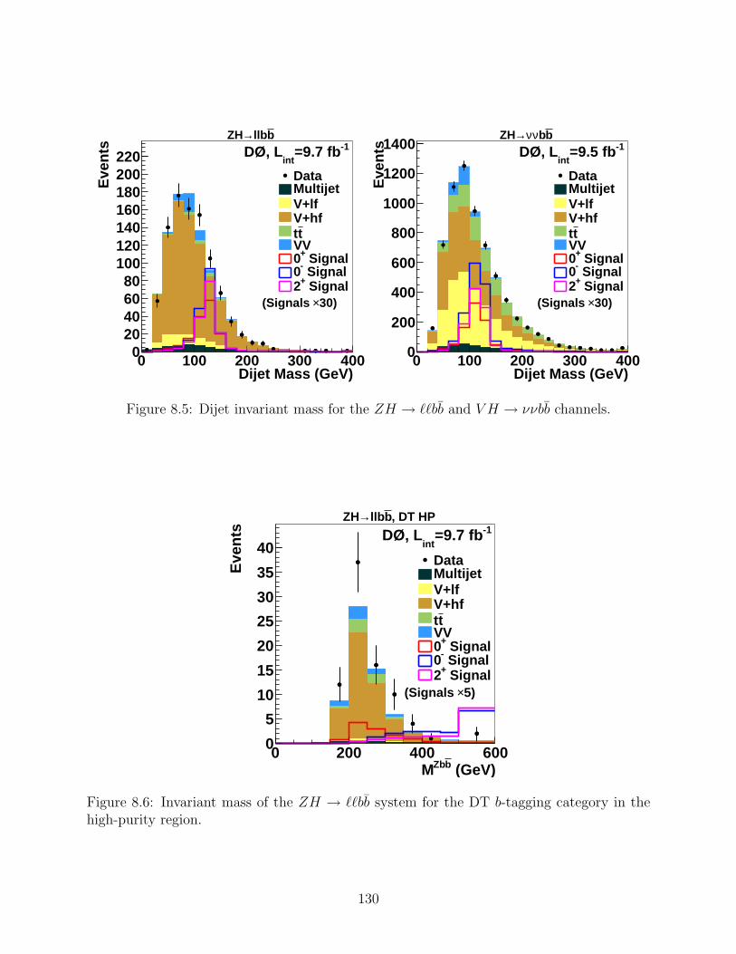
Dijet Mass (GeV)0 100 200 300 400

Eve

nts

020406080

100120140160180200220

-1=9.7 fbint

DØ, L

30)×(Signals

DataMultijetV+lfV+hftt

VV Signal+0 Signal-0 Signal+2

bllb→ZH

Dijet Mass (GeV)0 100 200 300 400

Eve

nts

0

200

400

600

800

1000

1200

1400 -1=9.5 fbint

DØ, L

30)×(Signals

DataMultijetV+lfV+hftt

VV Signal+0 Signal-0 Signal+2

bbνν→ZH

Figure 8.5: Dijet invariant mass for the ZH → ℓℓbb and V H → ννbb channels.

(GeV)bZbM0 200 400 600

Eve

nts

0

5

10

15

20

25

30

35

40-1=9.7 fb

intDØ, L

5)×(Signals

DataMultijetV+lfV+hftt

VV Signal+0 Signal-0 Signal+2

, DT HPbllb→ZH

Figure 8.6: Invariant mass of the ZH → ℓℓbb system for the DT b-tagging category in thehigh-purity region.

130

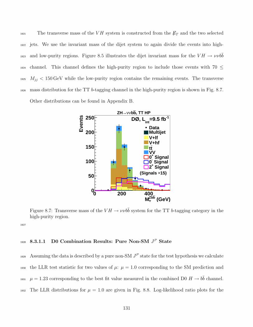
The transverse mass of the V H system is constructed from the 6ET and the two selected1921

jets. We use the invariant mass of the dijet system to again divide the events into high-1922

and low-purity regions. Figure 8.5 illustrates the dijet invariant mass for the V H → ννbb1923

channel. This channel defines the high-purity region to include those events with 70 ≤1924

Mjj < 150 GeV while the low-purity region contains the remaining events. The transverse1925

mass distribution for the TT b-tagging channel in the high-purity region is shown in Fig. 8.7.1926

Other distributions can be found in Appendix B.

(GeV)bZbTM

0 200 400

Eve

nts

0

50

100

150

200

250 -1=9.5 fbint

DØ, L

15)×(Signals

DataMultijetV+lfV+hftt

VV Signal+0 Signal-0 Signal+2

, TT HPbbνν→ZH

Figure 8.7: Transverse mass of the V H → ννbb system for the TT b-tagging category in thehigh-purity region.

1927

8.3.1.1 D0 Combination Results: Pure Non-SM JP State1928

Assuming the data is described by a pure non-SM JP state for the test hypothesis we calculate1929

the LLR test statistic for two values of µ: µ = 1.0 corresponding to the SM prediction and1930

µ = 1.23 corresponding to the best fit value measured in the combined D0 H → bb channel.1931

The LLR distributions for µ = 1.0 are given in Fig. 8.8. Log-likelihood ratio plots for the1932

131

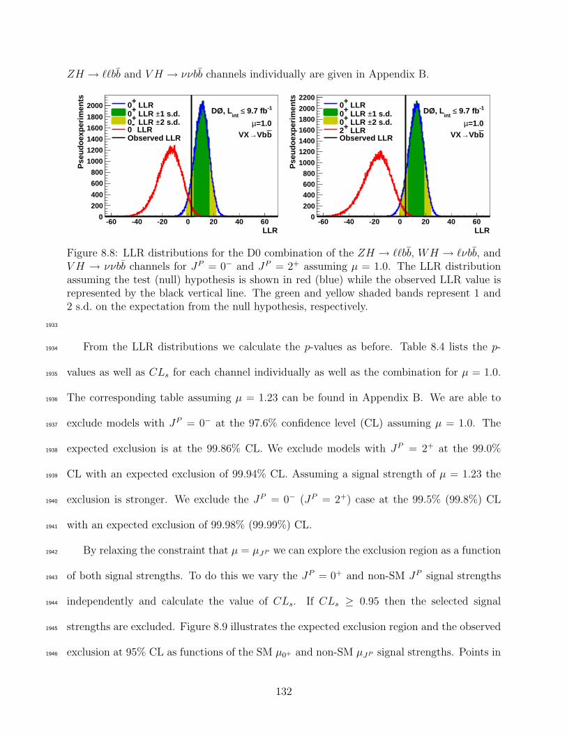
ZH → ℓℓbb and V H → ννbb channels individually are given in Appendix B.

LLR-60 -40 -20 0 20 40 60

Pse

udoe

xper

imen

ts

0

200

400

600

800

1000

1200

1400

1600

1800

2000 LLR+01 s.d.± LLR +02 s.d.± LLR +0

LLR-

0Observed LLR

-1 9.7 fb≤ int

DØ, L

=1.0µbVb→VX

LLR-60 -40 -20 0 20 40 60

Pse

udoe

xper

imen

ts

0

200

400

600

800

1000

1200

1400

1600

1800

2000

2200 LLR+0

1 s.d.± LLR +02 s.d.± LLR +0

LLR+2Observed LLR

-1 9.7 fb≤ int

DØ, L

=1.0µbVb→VX

Figure 8.8: LLR distributions for the D0 combination of the ZH → ℓℓbb, WH → ℓνbb, andV H → ννbb channels for JP = 0− and JP = 2+ assuming µ = 1.0. The LLR distributionassuming the test (null) hypothesis is shown in red (blue) while the observed LLR value isrepresented by the black vertical line. The green and yellow shaded bands represent 1 and2 s.d. on the expectation from the null hypothesis, respectively.

1933

From the LLR distributions we calculate the p-values as before. Table 8.4 lists the p-1934

values as well as CLs for each channel individually as well as the combination for µ = 1.0.1935

The corresponding table assuming µ = 1.23 can be found in Appendix B. We are able to1936

exclude models with JP = 0− at the 97.6% confidence level (CL) assuming µ = 1.0. The1937

expected exclusion is at the 99.86% CL. We exclude models with JP = 2+ at the 99.0%1938

CL with an expected exclusion of 99.94% CL. Assuming a signal strength of µ = 1.23 the1939

exclusion is stronger. We exclude the JP = 0− (JP = 2+) case at the 99.5% (99.8%) CL1940

with an expected exclusion of 99.98% (99.99%) CL.1941

By relaxing the constraint that µ = µJP we can explore the exclusion region as a function1942

of both signal strengths. To do this we vary the JP = 0+ and non-SM JP signal strengths1943

independently and calculate the value of CLs. If CLs ≥ 0.95 then the selected signal1944

strengths are excluded. Figure 8.9 illustrates the expected exclusion region and the observed1945

exclusion at 95% CL as functions of the SM µ0+ and non-SM µJP signal strengths. Points in1946

132

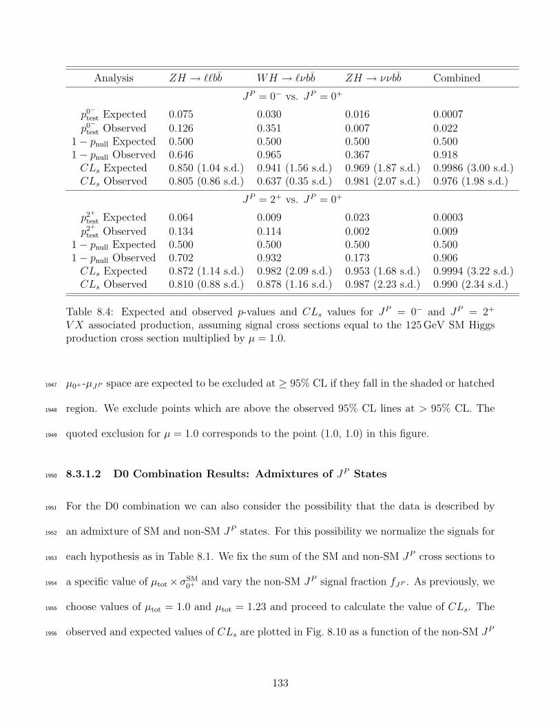
Analysis ZH → ℓℓbb WH → ℓνbb ZH → ννbb Combined

JP = 0− vs. JP = 0+

p0−

test Expected 0.075 0.030 0.016 0.0007

p0−

test Observed 0.126 0.351 0.007 0.0221 − pnull Expected 0.500 0.500 0.500 0.5001 − pnull Observed 0.646 0.965 0.367 0.918

CLs Expected 0.850 (1.04 s.d.) 0.941 (1.56 s.d.) 0.969 (1.87 s.d.) 0.9986 (3.00 s.d.)CLs Observed 0.805 (0.86 s.d.) 0.637 (0.35 s.d.) 0.981 (2.07 s.d.) 0.976 (1.98 s.d.)

JP = 2+ vs. JP = 0+

p2+

test Expected 0.064 0.009 0.023 0.0003

p2+

test Observed 0.134 0.114 0.002 0.0091 − pnull Expected 0.500 0.500 0.500 0.5001 − pnull Observed 0.702 0.932 0.173 0.906

CLs Expected 0.872 (1.14 s.d.) 0.982 (2.09 s.d.) 0.953 (1.68 s.d.) 0.9994 (3.22 s.d.)CLs Observed 0.810 (0.88 s.d.) 0.878 (1.16 s.d.) 0.987 (2.23 s.d.) 0.990 (2.34 s.d.)

Table 8.4: Expected and observed p-values and CLs values for JP = 0− and JP = 2+

V X associated production, assuming signal cross sections equal to the 125 GeV SM Higgsproduction cross section multiplied by µ = 1.0.

µ0+-µJP space are expected to be excluded at ≥ 95% CL if they fall in the shaded or hatched1947

region. We exclude points which are above the observed 95% CL lines at > 95% CL. The1948

quoted exclusion for µ = 1.0 corresponds to the point (1.0, 1.0) in this figure.1949

8.3.1.2 D0 Combination Results: Admixtures of JP States1950

For the D0 combination we can also consider the possibility that the data is described by1951

an admixture of SM and non-SM JP states. For this possibility we normalize the signals for1952

each hypothesis as in Table 8.1. We fix the sum of the SM and non-SM JP cross sections to1953

a specific value of µtot ×σSM0+ and vary the non-SM JP signal fraction fJP . As previously, we1954

choose values of µtot = 1.0 and µtot = 1.23 and proceed to calculate the value of CLs. The1955

observed and expected values of CLs are plotted in Fig. 8.10 as a function of the non-SM JP1956

133

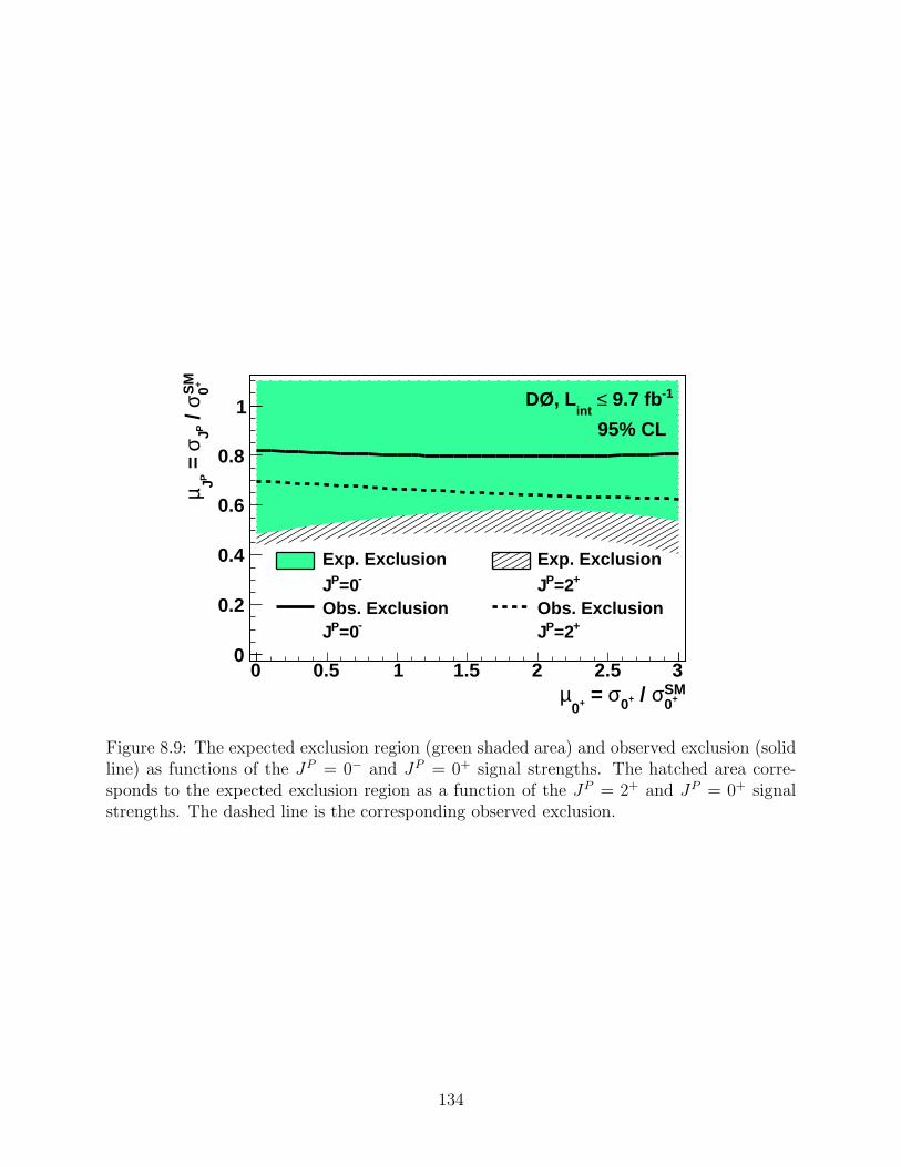
SM+0σ / +0σ = +0

µ0 0.5 1 1.5 2 2.5 3

SM + 0σ

/ P Jσ

=

P Jµ

0

0.2

0.4

0.6

0.8

1

Exp. Exclusion Exp. Exclusion-=0PJ +=2PJ

Obs. Exclusion Obs. Exclusion-=0PJ +=2PJ

-1 9.7 fb≤ int

DØ, L

95% CL

Figure 8.9: The expected exclusion region (green shaded area) and observed exclusion (solidline) as functions of the JP = 0− and JP = 0+ signal strengths. The hatched area corre-sponds to the expected exclusion region as a function of the JP = 2+ and JP = 0+ signalstrengths. The dashed line is the corresponding observed exclusion.

134

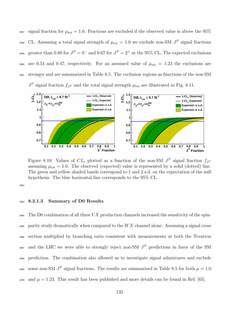
signal fraction for µtot = 1.0. Fractions are excluded if the observed value is above the 95%1957

CL. Assuming a total signal strength of µtot = 1.0 we exclude non-SM JP signal fractions1958

greater than 0.80 for JP = 0− and 0.67 for JP = 2+ at the 95% CL. The expected exclusions1959

are 0.54 and 0.47, respectively. For an assumed value of µtot = 1.23 the exclusions are1960

stronger and are summarized in Table 8.5. The exclusion regions as functions of the non-SM1961

JP signal fraction fJP and the total signal strength µtot are illustrated in Fig. 8.11.

Fraction-

00.1 0.2 0.3 0.4 0.5 0.6 0.7 0.8 0.9 1

s1-

CL

0.7

0.8

0.9

1

1.1

1.2

1.3-1 9.7 fb≤

intDØ, L

SMHσ=+0

σ+-0σ

Observeds1-CL

Expecteds1-CL

1 s.d.±Expected

2 s.d.±Expected

Fraction+20.1 0.2 0.3 0.4 0.5 0.6 0.7 0.8 0.9 1

s1-

CL

0.7

0.8

0.9

1

1.1

1.2

1.3-1 9.7 fb≤

intDØ, L

SMHσ=+0

σ++2σ

Observeds1-CL

Expecteds1-CL

1 s.d.±Expected

2 s.d.±Expected

Figure 8.10: Values of CLs plotted as a function of the non-SM JP signal fraction fJP

assuming µtot = 1.0. The observed (expected) value is represented by a solid (dotted) line.The green and yellow shaded bands correspond to 1 and 2 s.d. on the expectation of the nullhypothesis. The blue horizontal line corresponds to the 95% CL.

1962

8.3.1.3 Summary of D0 Results1963

The D0 combination of all three V X production channels increased the sensitivity of the spin-1964

parity study dramatically when compared to the WX channel alone. Assuming a signal cross1965

section multiplied by branching ratio consistent with measurements at both the Tevatron1966

and the LHC we were able to strongly reject non-SM JP predictions in favor of the SM1967

prediction. The combination also allowed us to investigate signal admixtures and exclude1968

some non-SM JP signal fractions. The results are summarized in Table 8.5 for both µ = 1.01969

and µ = 1.23. This result has been published and more details can be found in Ref. [65].1970

135

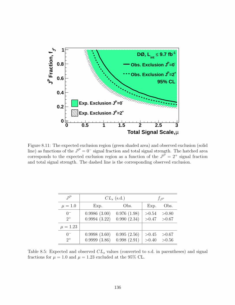
µTotal Signal Scale, 0 0.5 1 1.5 2 2.5 3

P J F

ract

ion,

fP J

0

0.2

0.4

0.6

0.8

1

-=0PExp. Exclusion J

+=2PExp. Exclusion J

-=0PObs. Exclusion J

+=2PObs. Exclusion J

-1 9.7 fb≤ int

DØ, L

95% CL

Figure 8.11: The expected exclusion region (green shaded area) and observed exclusion (solidline) as functions of the JP = 0− signal fraction and total signal strength. The hatched areacorresponds to the expected exclusion region as a function of the JP = 2+ signal fractionand total signal strength. The dashed line is the corresponding observed exclusion.

JP CLs (s.d.) fJP

µ = 1.0 Exp. Obs. Exp. Obs.

0− 0.9986 (3.00) 0.976 (1.98) >0.54 >0.802+ 0.9994 (3.22) 0.990 (2.34) >0.47 >0.67

µ = 1.23

0− 0.9998 (3.60) 0.995 (2.56) >0.45 >0.672+ 0.9999 (3.86) 0.998 (2.91) >0.40 >0.56

Table 8.5: Expected and observed CLs values (converted to s.d. in parentheses) and signalfractions for µ = 1.0 and µ = 1.23 excluded at the 95% CL.

136

8.3.2 Tevatron Combination1971

The statistical combination of our results with those of a similar study at the CDF experiment[66]1972

will increase the potential exclusion region. All three V X production channels were studied1973

at the CDF experiment using the method suggested by [38]. The analysis method for the1974

individual channels is similar to what was done at the D0 experiment and are briefly de-1975

scribed in the following. All analyses use the same multivariate classifier to tag b quark jets.1976

The classifier does not perform well on jets with ET > 200 GeV so b-tagging is not applied1977

for these jets in all channels. For the spin-parity analysis a multivariate analysis (MVA) tool1978

was trained to discriminate between the SM backgrounds and the non-SM JP signal. Events1979

that are classified as background are then classified using the MVA for the SM Higgs boson1980

search in the WH → ℓνbb and V H → ννbb channels. Detailed descriptions of the SM Higgs1981

boson searches on which the current analyses are based can be found in [67, 40, 68]. It is1982

interesting to note that the CDF experiment reported 1 s.d. and 2 s.d. deficits in the signal1983

regions for the JP = 0− and JP = 2+ hypotheses, respectively. This is in contrast to the1984

results of the D0 study which had a 2 s.d. excess. The combination of these results will have1985

the effect of balancing the two extremes. The details of the Tevatron combination have been1986

published and more information can be found in Ref. [69].1987

ZH → ℓℓbb Channel (CDF)1988

This channel requires two isolated leptons and at least two jets. The CDF analysis1989

of this channel requires either two or three jets. Events are divided into b-tagging1990

categories based on the output of a multivariate classifier. For the ZH → ℓℓbb channel1991

they use three double-b-tag categories and one single-b-tag category.1992

WH → ℓνbb Channel (CDF)1993

137

CDF requires one lepton (e or µ), exactly two jets, and significant 6ET . Events are1994

classified according to the quality of the selected lepton. These are high-quality leptons1995

in the central detector, leptons based on isolated tracks, and electrons in the forward1996

region. They define five b-tagging categories: three double-b-tag categories and two1997

single-b-tag categories.1998

V H → ννbb Channel (CDF)1999

The V H → ννbb channel selects events with large 6ET and two or three jets. The2000

jets are divided into two double-b-tag categories and one single-b-tag category. This2001

analysis is also sensitive to WH → ℓνbb production where the lepton is not identified.2002

8.3.2.1 Tevatron Combination Results: Pure Non-SM JP State2003

For the Tevatron combination we first assume a pure non-SM JP state and again calculate2004

the value of CLs assuming µ = 1.0. The LLR distributions for JP = 0− and JP = 2+ are2005

shown in Fig. 8.12. The calculated 1 − CLs values are presented in Table 8.6. We exclude2006

models with non-SM JP signals with significances of 5.0 s.d. and 4.9 s.d. for the JP = 0−2007

and JP = 2+ hypotheses, respectively. The expected significances for the JP = 0− and2008

JP = 2+ hypotheses are 4.8 s.d. and 4.6 s.d. In the Tevatron combination the observed2009

significances are higher than expected. This effect is driven by a deficit in the observed2010

number of events in a region with high non-SM JP signal content for the CDF analyses. The2011

largest contribution comes from the WX → ℓνbb channel.2012

8.3.2.2 Tevatron Combination Results: Admixtures of JP States2013

The Tevatron combination also considers the possibility of signal admixtures. We explore the2014

exclusion regions as functions of the non-SM JP signal fraction and the total signal strength.2015

138

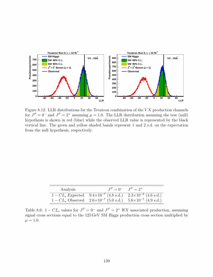
LLR-80 -60 -40 -20 0 20 40 60

Pse

udoe

xper

imen

ts

0

100

200

300

400

500

600

700SM Higgs

68% C.L.SM

95% C.L.SM

= 1) µ Boson (-

JP = 0

Observed

-1 10 fb≤Tevatron Run II, L

bVb→VX

LLR-80 -60 -40 -20 0 20 40 60

Pse

udoe

xper

imen

ts

0

100

200

300

400

500

600

700

800

900SM Higgs

68% C.L.SM

95% C.L.SM

= 1) µ Boson (+

JP = 2

Observed

-1 10 fb≤Tevatron Run II, L

bVb→VX

Figure 8.12: LLR distributions for the Tevatron combination of the V X production channelsfor JP = 0− and JP = 2+ assuming µ = 1.0. The LLR distribution assuming the test (null)hypothesis is shown in red (blue) while the observed LLR value is represented by the blackvertical line. The green and yellow shaded bands represent 1 and 2 s.d. on the expectationfrom the null hypothesis, respectively.

Analysis JP = 0− JP = 2+

1 − CLs Expected 9.4×10−7 (4.8 s.d.) 2.3×10−6 (4.6 s.d.)1 − CLs Observed 2.6×10−7 (5.0 s.d.) 5.6×10−7 (4.9 s.d.)

Table 8.6: 1 − CLs values for JP = 0− and JP = 2+ WX associated production, assumingsignal cross sections equal to the 125 GeV SM Higgs production cross section multiplied byµ = 1.0.

139

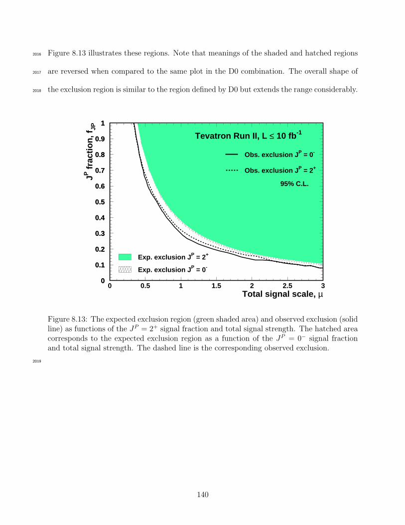
Figure 8.13 illustrates these regions. Note that meanings of the shaded and hatched regions2016

are reversed when compared to the same plot in the D0 combination. The overall shape of2017

the exclusion region is similar to the region defined by D0 but extends the range considerably.2018

0

0.1

0.2

0.3

0.4

0.5

0.6

0.7

0.8

0.9

1

0 0.5 1 1.5 2 2.5 30

0.1

0.2

0.3

0.4

0.5

0.6

0.7

0.8

0.9

1

Total signal scale, µ

JP fr

actio

n, f

JP

Tevatron Run II, L ≤ 10 fb -1

Obs. exclusion J P = 0-

Obs. exclusion J P = 2+

95% C.L.

Exp. exclusion J P = 0-

Exp. exclusion J P = 2+

Figure 8.13: The expected exclusion region (green shaded area) and observed exclusion (solidline) as functions of the JP = 2+ signal fraction and total signal strength. The hatched areacorresponds to the expected exclusion region as a function of the JP = 0− signal fractionand total signal strength. The dashed line is the corresponding observed exclusion.

2019

140

Chapter 92020

Conclusion2021

Beginning with the recommendation of Ref. [38] to study the JP character of the excess2022

observed at the Tevatron we were able to exclude models for the Higgs boson with exotic spin2023

and parity with high significance. We studied WH production where the W boson decays2024

leptonically and the Higgs boson decays to a pair of b quarks in detail. Using the transverse2025

mass of the WH system as a discrimination tool we investigated two well-motivated JP2026

states: JP = 0− and JP = 2+. Assuming that the signal cross sections were equal to the2027

125 GeV SM Higgs boson production cross section multiplied by µ = 1.0 we found that we2028

could not exclude these possibilities at the 95% CL. By combining the other vector boson2029

associated production channels at D0 we were able to exclude the JP = 0− and JP = 2+2030

hypotheses at the 97.6% CL and 99.0% CL, respectively. We considered the possibility2031

that the data is described by an admixture of SM and non-SM JP states. We were able2032

to exclude JP = 0− signal fractions f0− > 0.80 and JP = 2+ signal fractions f2+ > 0.672033

at the 95% CL. We also combined our results with the results of the CDF experiment.2034

The JP = 0− and JP = 2+ hypotheses are excluded with significances of 5.0 s.d. and2035

4.9 s.d., respectively. The corresponding confidence levels are > 99.9999%. At the time of2036

this writing, these production channels are not accessible to the experiments at the LHC2037

because of the relatively low signal-to-background ratio. These results are the most stringent2038

exclusions of models for the Higgs boson with exotic spin and parity in a fermionic Higgs2039

boson decay channel and will remain so until the LHC acquires the necessary sensitivity.2040

141

APPENDICES2041

142

Appendix A2042

Experimental Apparatus Details2043

This appendix gives more detail on the experimental equipment used to produce and record2044

the data. The Fermilab accelerator chain is described in Section A.1. Additional information2045

on the hardware and software of the D0 detector is given in Section A.2.2046

A.1 Fermilab Accelerator Chain2047

The following describes the Fermilab accelerator chain from the production of protons and2048

antiprotons to the collisions at a center of mass energy of 1.96TeV.2049

A.1.1 Life of a Proton2050

A.1.1.1 The Preaccelerator2051

All protons at Fermilab begin in a bottle of hydrogen gas at one of two preaccelerators.2052

There are two for redundancy and can be considered identical for the purpose of this Thesis.2053

Each preaccelerator consists of a negative hydrogen ion source, a Cockcroft-Walton voltage2054

generator, an electrostatic accelerating column, and a transport line for injection into the2055

Linac.2056

To begin, hydrogen gas is pumped into a surface plasma magnetron source. The mag-2057

netron source, Fig. A.1, consists of a oval shaped cathode surrounded by an anode and placed2058

in a magnetic field parallel to the cathode surface. The anode and cathode are energized2059

143

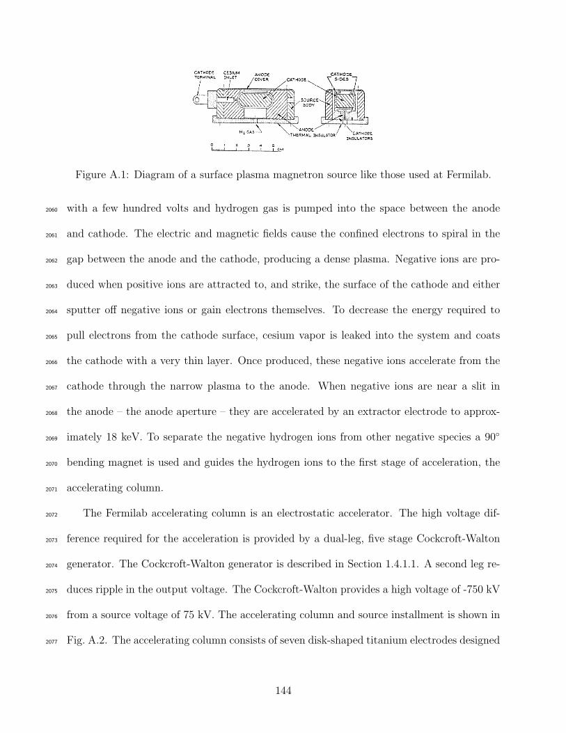
Figure A.1: Diagram of a surface plasma magnetron source like those used at Fermilab.

with a few hundred volts and hydrogen gas is pumped into the space between the anode2060

and cathode. The electric and magnetic fields cause the confined electrons to spiral in the2061

gap between the anode and the cathode, producing a dense plasma. Negative ions are pro-2062

duced when positive ions are attracted to, and strike, the surface of the cathode and either2063

sputter off negative ions or gain electrons themselves. To decrease the energy required to2064

pull electrons from the cathode surface, cesium vapor is leaked into the system and coats2065

the cathode with a very thin layer. Once produced, these negative ions accelerate from the2066

cathode through the narrow plasma to the anode. When negative ions are near a slit in2067

the anode – the anode aperture – they are accelerated by an extractor electrode to approx-2068

imately 18 keV. To separate the negative hydrogen ions from other negative species a 902069

bending magnet is used and guides the hydrogen ions to the first stage of acceleration, the2070

accelerating column.2071

The Fermilab accelerating column is an electrostatic accelerator. The high voltage dif-2072

ference required for the acceleration is provided by a dual-leg, five stage Cockcroft-Walton2073

generator. The Cockcroft-Walton generator is described in Section 1.4.1.1. A second leg re-2074

duces ripple in the output voltage. The Cockcroft-Walton provides a high voltage of -750 kV2075

from a source voltage of 75 kV. The accelerating column and source installment is shown in2076

Fig. A.2. The accelerating column consists of seven disk-shaped titanium electrodes designed2077

144

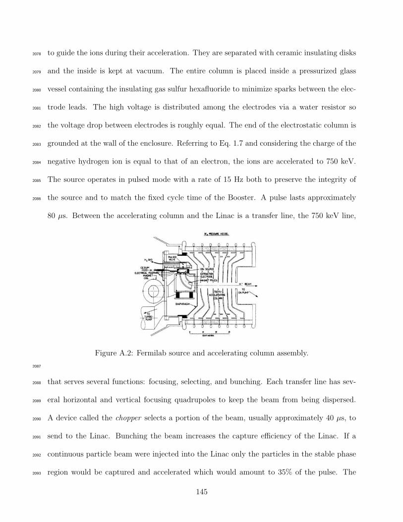
to guide the ions during their acceleration. They are separated with ceramic insulating disks2078

and the inside is kept at vacuum. The entire column is placed inside a pressurized glass2079

vessel containing the insulating gas sulfur hexafluoride to minimize sparks between the elec-2080

trode leads. The high voltage is distributed among the electrodes via a water resistor so2081

the voltage drop between electrodes is roughly equal. The end of the electrostatic column is2082

grounded at the wall of the enclosure. Referring to Eq. 1.7 and considering the charge of the2083

negative hydrogen ion is equal to that of an electron, the ions are accelerated to 750 keV.2084

The source operates in pulsed mode with a rate of 15 Hz both to preserve the integrity of2085

the source and to match the fixed cycle time of the Booster. A pulse lasts approximately2086

80 µs. Between the accelerating column and the Linac is a transfer line, the 750 keV line,

Figure A.2: Fermilab source and accelerating column assembly.

2087

that serves several functions: focusing, selecting, and bunching. Each transfer line has sev-2088

eral horizontal and vertical focusing quadrupoles to keep the beam from being dispersed.2089

A device called the chopper selects a portion of the beam, usually approximately 40 µs, to2090

send to the Linac. Bunching the beam increases the capture efficiency of the Linac. If a2091

continuous particle beam were injected into the Linac only the particles in the stable phase2092

region would be captured and accelerated which would amount to 35% of the pulse. The2093

145

buncher is a single-gap radio frequency cavity similar to the cavities in the Linac. It operates2094

at the same frequency as the Linac but with a different phase. Particles that arrive early2095

are decelerated and particles that arrive late are accelerated. This effectively decreases the2096

particles’ width in time but increases the particles’ momentum spread. With the buncher,2097

the Linac capture rate is approximately 70%.2098

A.1.1.2 The Linac2099

The Fermilab Linac is composed of two different machines that work in tandem to accelerate2100

the beam to 400 MeV. The first machine is an Alvarez drift tube linac (DTL). It consists of2101

five cylindrical oxygen-free high conductivity (OFHC) copper clad steel tanks. Each tank is2102

powered by its own 5 MW power source and resonates at 201.24 MHz. Each cavity has several2103

resonant cells extending from the center of one drift tube to the next with the cell length2104

ranging in length from 6.04 cm to 67.9 cm. The phase shift between adjacent accelerating2105

cells is zero and each RF bucket contains a particle bunch. The average axial electric field2106

ranges from 1.6 MV/m to 2.6 MV/m. This portion of the Linac accelerates the negative2107

hydrogen ions to 116 MeV.2108

After acceleration in the DTL the H− ions move into the second portion of the Linac,2109

the side-coupled linac (SCL). Instead of one cavity containing multiple accelerating cells as2110

in the DTL, each cavity is one cell in the SCL. The SCL consists of seven modules which are2111

divided into four sections with sixteen accelerating cells and fifteen coupling cells. Each cell2112

has a π/2 phase shift from each adjacent cell, giving a phase shift of π between accelerating2113

cells. Individual modules are powered with a single 12 MW power source and resonate at2114

804.96 MHz. Because the driving frequency is four times that of the DTL and the phase2115

shift between accelerating cells is different by π, the bunches travel eight accelerating cells2116

146

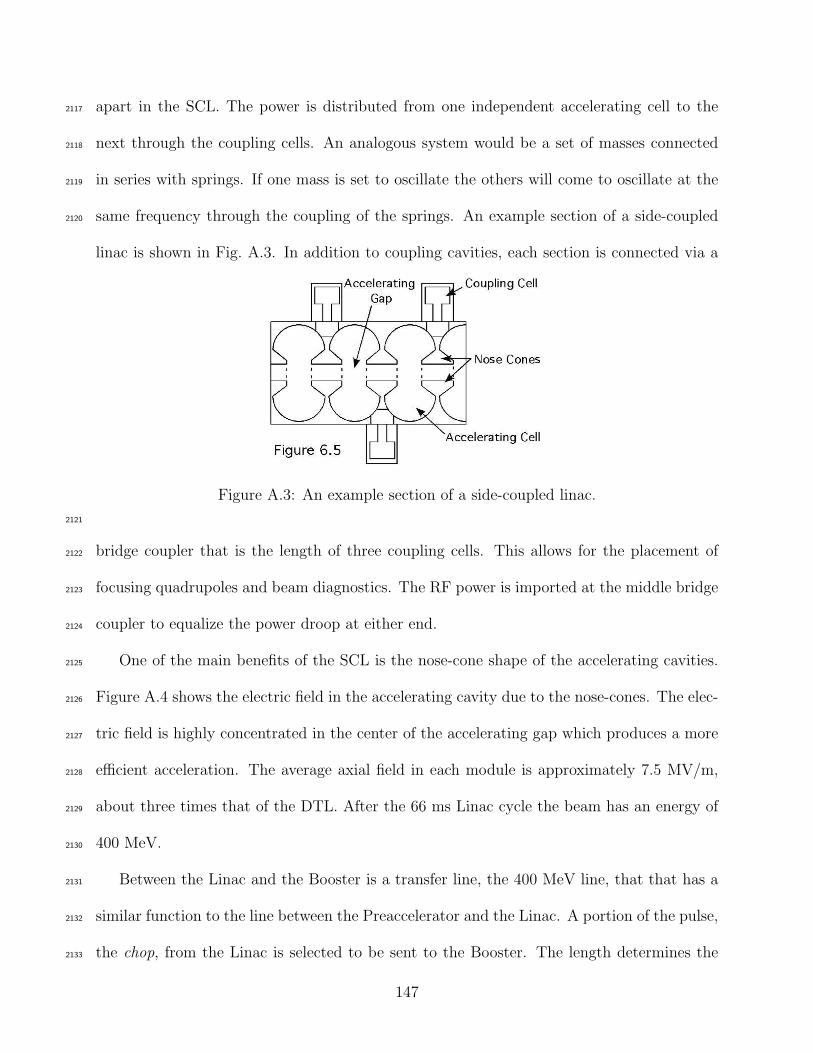
apart in the SCL. The power is distributed from one independent accelerating cell to the2117

next through the coupling cells. An analogous system would be a set of masses connected2118

in series with springs. If one mass is set to oscillate the others will come to oscillate at the2119

same frequency through the coupling of the springs. An example section of a side-coupled2120

linac is shown in Fig. A.3. In addition to coupling cavities, each section is connected via a

Figure A.3: An example section of a side-coupled linac.

2121

bridge coupler that is the length of three coupling cells. This allows for the placement of2122

focusing quadrupoles and beam diagnostics. The RF power is imported at the middle bridge2123

coupler to equalize the power droop at either end.2124

One of the main benefits of the SCL is the nose-cone shape of the accelerating cavities.2125

Figure A.4 shows the electric field in the accelerating cavity due to the nose-cones. The elec-2126

tric field is highly concentrated in the center of the accelerating gap which produces a more2127

efficient acceleration. The average axial field in each module is approximately 7.5 MV/m,2128

about three times that of the DTL. After the 66 ms Linac cycle the beam has an energy of2129

400 MeV.2130

Between the Linac and the Booster is a transfer line, the 400 MeV line, that that has a2131

similar function to the line between the Preaccelerator and the Linac. A portion of the pulse,2132

the chop, from the Linac is selected to be sent to the Booster. The length determines the2133

147

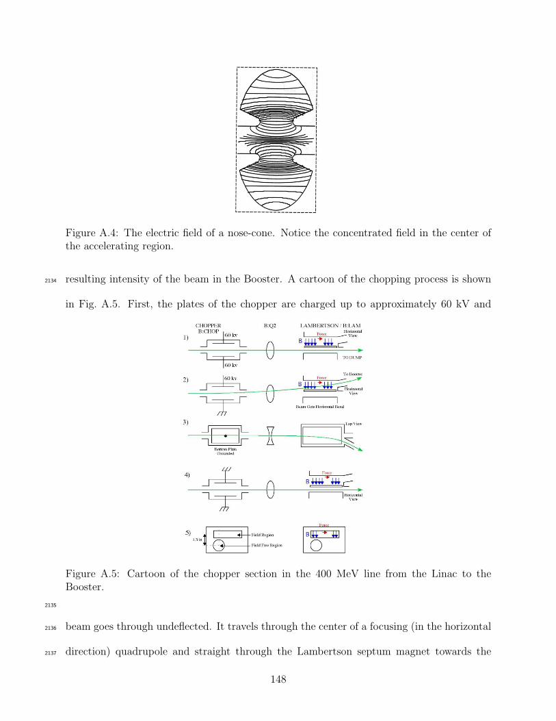
Figure A.4: The electric field of a nose-cone. Notice the concentrated field in the center ofthe accelerating region.

resulting intensity of the beam in the Booster. A cartoon of the chopping process is shown2134

in Fig. A.5. First, the plates of the chopper are charged up to approximately 60 kV and

Figure A.5: Cartoon of the chopper section in the 400 MeV line from the Linac to theBooster.

2135

beam goes through undeflected. It travels through the center of a focusing (in the horizontal2136

direction) quadrupole and straight through the Lambertson septum magnet towards the2137

148

beam dump. At the start of the chop the lower plate is grounded and the beam is deflected2138

upwards. It enters the quadrupole off-center and gets further deflected into the field region2139

of the Lambertson. The Lambertson gives the beam a horizontal bend of approximately 11.2140

At the end of the chop the top chopper plate is grounded and the remaining beam is again2141

undeflected and is sent to the beam dump. After the chop is selected it is sent down fifteen2142

feet to the Booster at an angle of approximately 13. After being kicked out of the SCL,2143

the beam passes through a debuncher which helps remove the 804.96 MHz RF structure2144

from the SCL and reduce the momentum spread in the beam. In addition to focusing and2145

steering magnets, the 400 MeV line must also match the lattice of the SCL to the lattice of2146

the Booster for efficient transfer.2147

A.1.1.3 The Booster2148

The Booster is the first in a series of three synchrotrons in the Fermilab accelerator chain. It2149

is a fast-cycling machine that completes a cycle from injection to extraction in roughly 66 ms.2150

It has a circumference of 468 m and consists of 96 combined function magnets arranged in2151

a FOFDOOD lattice: focusing quadrupole, short drift length, focusing quadrupole, defo-2152

cusing quadrupole, long drift length, and another defocusing quadrupole. It has seventeen2153

accelerating cavities located in the long drift sections.2154

At the injection energy of 400 MeV one turn in the Booster takes 2.22 µs. With a chop2155

length of approximately 40 µs, the beam from the Linac could wrap around the Booster2156

eighteen times! It is here that the benefit of starting with negative hydrogen ions is apparent.2157

If the source produced protons it would only be possible to fill up one turn of the Booster.2158

In this way the intensity of the beam is limited and a large amount of beam is wasted. A2159

clever route was taken to solve this problem and is shown in Fig. A.6. Upon injection, the2160

149

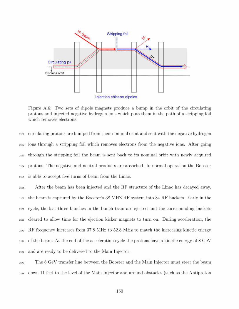
Figure A.6: Two sets of dipole magnets produce a bump in the orbit of the circulatingprotons and injected negative hydrogen ions which puts them in the path of a stripping foilwhich removes electrons.

circulating protons are bumped from their nominal orbit and sent with the negative hydrogen2161

ions through a stripping foil which removes electrons from the negative ions. After going2162

through the stripping foil the beam is sent back to its nominal orbit with newly acquired2163

protons. The negative and neutral products are absorbed. In normal operation the Booster2164

is able to accept five turns of beam from the Linac.2165

After the beam has been injected and the RF structure of the Linac has decayed away,2166

the beam is captured by the Booster’s 38 MHZ RF system into 84 RF buckets. Early in the2167

cycle, the last three bunches in the bunch train are ejected and the corresponding buckets2168

cleared to allow time for the ejection kicker magnets to turn on. During acceleration, the2169

RF frequency increases from 37.8 MHz to 52.8 MHz to match the increasing kinetic energy2170

of the beam. At the end of the acceleration cycle the protons have a kinetic energy of 8 GeV2171

and are ready to be delivered to the Main Injector.2172

The 8 GeV transfer line between the Booster and the Main Injector must steer the beam2173

down 11 feet to the level of the Main Injector and around obstacles (such as the Antiproton2174

150

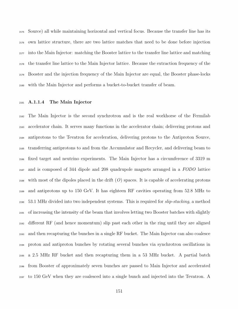
Source) all while maintaining horizontal and vertical focus. Because the transfer line has its2175

own lattice structure, there are two lattice matches that need to be done before injection2176

into the Main Injector: matching the Booster lattice to the transfer line lattice and matching2177

the transfer line lattice to the Main Injector lattice. Because the extraction frequency of the2178

Booster and the injection frequency of the Main Injector are equal, the Booster phase-locks2179

with the Main Injector and performs a bucket-to-bucket transfer of beam.2180

A.1.1.4 The Main Injector2181

The Main Injector is the second synchrotron and is the real workhorse of the Fermilab2182

accelerator chain. It serves many functions in the accelerator chain; delivering protons and2183

antiprotons to the Tevatron for acceleration, delivering protons to the Antiproton Source,2184

transferring antiprotons to and from the Accumulator and Recycler, and delivering beam to2185

fixed target and neutrino experiments. The Main Injector has a circumference of 3319 m2186

and is composed of 344 dipole and 208 quadrupole magnets arranged in a FODO lattice2187

with most of the dipoles placed in the drift (O) spaces. It is capable of accelerating protons2188

and antiprotons up to 150 GeV. It has eighteen RF cavities operating from 52.8 MHz to2189

53.1 MHz divided into two independent systems. This is required for slip-stacking, a method2190

of increasing the intensity of the beam that involves letting two Booster batches with slightly2191

different RF (and hence momentum) slip past each other in the ring until they are aligned2192

and then recapturing the bunches in a single RF bucket. The Main Injector can also coalesce2193

proton and antiproton bunches by rotating several bunches via synchrotron oscillations in2194

a 2.5 MHz RF bucket and then recapturing them in a 53 MHz bucket. A partial batch2195

from Booster of approximately seven bunches are passed to Main Injector and accelerated2196

to 150 GeV when they are coalesced into a single bunch and injected into the Tevatron. A2197

151

total of 36 of these super bunches are injected into the Tevatron for collisions.2198

A.1.1.5 The Tevatron2199

The Tevatron is the third synchrotron and final accelerator in the chain. It is a super-2200

conducting synchrotron that is 6.3 km in circumference. Over a thousand superconducting2201

magnets cooled to liquid helium temperatures make up the FODO lattice of the Tevatron.2202

Unlike the other machines which serve a variety of purposes throughout the complex, the2203

Tevatron has one mode of operation: collider mode. Its job is to accelerate counter-rotating2204

protons and antiprotons to their final energy of 980 GeV and then collide them at two fixed2205

points around the ring. Once the acceleration is complete, it functions as a storage ring2206

where stable beams collide for hours on end. There are eight accelerating cavities which2207

resonate from 53.103 MHz to 53.104 MHz during acceleration. The acceleration of both pro-2208

tons and antiprotons in this machine requires two independent RF systems to allow for fine2209

control over the relative positions of the beams. The eight accelerating cavities are divided2210

into two groups: one that accelerates the protons and one that accelerates the antiprotons.2211

The Tevatron now has 36 coalesced bunches of protons circulating at the injection energy of2212

150 GeV. We will return to the Tevatron later when discussing antiprotons.2213

A.1.2 Life of an Antiproton2214

Antiprotons are more difficult to make and many aspects of the accelerator chain reflect2215

this. To get an idea of how difficult it is to produce antiprotons consider that for every 1052216

protons that bombard the target only about two antiprotons are produced. The Fermilab2217

Antiproton Source consists of the Target Vault, two triangular synchrotrons: the Debuncher2218

and the Accumulator, and a permanent-magnet storage ring called the Recycler. The Main2219

152

Injector and the Tevatron are also directly involved in the acceleration and transport of2220

the antiprotons. To begin, Booster sends two batches of protons to Main Injector where2221

they are slip-stacked and accelerated to 120 GeV. Main Injector then rotates the bunches2222

in longitudinal phase space, creating bunches which have a large momentum spread but a2223

small spread in time. The bunches are then extracted from the Main Injector and sent to2224

the Target Vault.2225

A.1.2.1 Target Vault2226

Upstream of the target is a sweeper magnet, a rotating dipole which deflects the proton beam2227

in a circle to reduce heating of the target. The protons impinge on an Inconel (a nickel-iron2228

alloy) target which produces a spray of secondary particles some of which are antiprotons.2229

The target is cylindrical in shape and rotates on an axis perpendicular to the incoming2230

beam to reduce target heating and degradation. Immediately after the target is a lithium2231

lens which focuses the secondaries in both transverse planes. Lithium is used because it is the2232

least dense solid conductor; scattering and absorption of the rare antiprotons is minimized.2233

A copper collimator with a hole bored in the center for the beam to travel through protects2234

the next element, a pulsed dipole magnet. This magnet selects negatively-charged 8 GeV2235

secondaries and sends them to the Debuncher.2236

A.1.2.2 The Debuncher2237

The Debuncher is a rounded triangle synchrotron with a traditional FODO lattice. It oper-2238

ates at a fixed energy of 8 GeV, the peak energy of the Booster and close to the antiproton2239

production peak. As the name implies, its function is to debunch the incoming antiprotons.2240

During the transit from the Target Vault most of the secondaries that were not antiprotons2241

153

decayed away and the rest will be lost during the first few trips around the Debuncher. The2242

antiprotons that are left have retained the bunch structure of the protons that left the Main2243

Injector. The main RF system in the Debuncher is a 53.1 MHz system that is responsible for2244

rotating the beam of antiprotons in longitudinal phase space to recreate bunches that have2245

a large spread in time and a small momentum spread. It is also responsible for debunching2246

the beam. A secondary RF system maintains a gap between the head and tail of the bunch2247

train so the train fits around the smaller Accumulator ring. The Debuncher uses stochas-2248

tic cooling of the beam to decrease the transverse and longitudinal emittance resulting in2249

a denser particle beam. Stochastic cooling uses sets of pick-ups and kickers to detect and2250

correct errors in the beam energy and transverse displacement.2251

A.1.2.3 The Accumulator2252

The Accumulator is an 8 GeV fixed-energy synchrotron in the shape of a triangle with flat-2253

tened corners. It lies on the inside radius in the same tunnel as the Debuncher and has2254

a similar FODO lattice. The Accumulator collects successive antiproton batches from the2255

Debuncher over several hours. It performs momentum stacking where newly injected beam2256

is cooled and decelerated towards a core momentum value. Figure A.7 shows the radial2257

distribution of antiprotons, collectively called the stack, in the Accumulator. Antiprotons2258

of lower energy occupy a smaller radius in the machine. There is a difference in energy of2259

150 MeV from the stack core to the injection orbit. This is accomplished in the Accumulator2260

first through RF manipulations and then through stochastic cooling. Beam from the De-2261

buncher is a continuous ribbon and is captured into 53 MHz buckets and decelerated 60 MeV2262

and deposited at the edge of the stack tail. The RF voltage is lowered slowly to allow the2263

beam to debunch. Stack tail cooling systems are momentum cooling systems with pick-ups2264

154

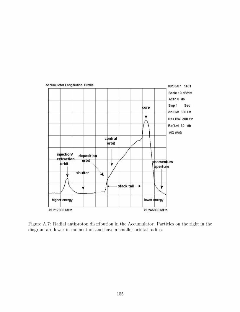
Figure A.7: Radial antiproton distribution in the Accumulator. Particles on the right in thediagram are lower in momentum and have a smaller orbital radius.

155

in high dispersion sections. These cooling systems decelerate the beam to the core region in2265

approximately twenty minutes. Once in the core region, momentum cooling systems keep2266

the beam contained in the core by decelerating higher momentum particles and accelerating2267

lower momentum particles to keep them inside the machine. Transverse cooling pickups2268

for the core are located in low dispersion sections and are used to control the transverse2269

emittance.2270

Once a stack of suitable intensity is reached, part of the core is extracted from the2271

Accumulator and transferred to the Recycler by the Main Injector. A 2.52 MHz RF system2272

creates four bunches from the core and slowly accelerates them through the rest of the stack2273

and all the way to the extraction orbit. They are then kicked out of the Accumulator without2274

disturbing the rest of the stack and transferred by the Main Injector to the Recycler.2275

A.1.2.4 The Recycler2276

The Recycler is an 8 GeV storage ring. It consists of permanent combined function magnets2277

arranged in a FODO lattice. It resides above the Main Injector in the same tunnel. Like2278

the Accumulator its job is to accumulate and store antiprotons. It accepts several batches2279

of antiprotons from the Accumulator and is capable of storing them for hours. In the2280

Recycler the accumulated antiprotons are referred to as the stash to differentiate from the2281

Accumulator’s stack.2282

Like the Accumulator and Debuncher, the Recycler uses stochastic cooling to control2283

both the transverse and longitudinal emittance. Unlike these machines, the Recycler also2284

uses electron cooling to decrease the momentum spread. In this scheme an electron gun2285

produces a highly collimated and nearly monochromatic electron beam which is accelerated2286

to match the average velocity of the circulating antiprotons. This electron beam is then2287

156

allowed to travel alongside the antiproton beam for a short distance. Along the way, energy2288

from the ‘hot’ antiprotons is transferred to the ‘cold’ electrons. The electrons are then2289

returned to the source taking the energy gained with them.2290

So far we’ve seen beam stored in two different ways: in bunches or in a continuous2291

ribbon. The Recycler stores its beam in a different manner. Instead of using a resonant2292

RF cavity it uses a wide-band RF cavity that is capable of producing a multitude of (non-2293

resonant) waveforms. The most used waveform in the Recycler is a rectangular pulse. Beam2294

is stored longitudinally between a negative and a positive voltage pulse called a barrier2295

bucket. All other manipulations of the beam are done using additional rectangular pulses.2296

During injection, the four bunches of antiprotons from the Main Injector are captured by a2297

2.5 MHz sinusoidal waveform which is contained inside a barrier bucket. The gain on the2298

waveform is reduced and the beam is allowed to debunch inside the barrier bucket. This2299

barrier bucket is then moved towards the stash and the barriers between them are removed.2300

When the Recycler intensity is great enough and the Tevatron is ready to start a new store2301

the antiprotons are longitudinally ‘momentum-mined’. Another set of RF manipulations2302

creates nine parcels of low momentum spread. These parcels are moved one by one to the2303

extraction region where they are made into four bunches and sent to the Main Injector for2304

acceleration.2305

A.1.2.5 The Main Injector: An Antiproton’s Point of View2306

After injecting 36 coalesced proton bunches into the Tevatron one at a time, Main Injector2307

can begin accepting antiprotons from the Recycler. Because antiprotons have the same mass2308

but opposite charge as the protons, the lattice of the Main Injector also works to accelerate2309

157

antiprotons as long as their direction of travel is opposite that of the protons.1 The Main2310

Injector accepts four bunches from the Recycler equal to one parcel or 1/9 of the stash. It2311

accelerates these four bunches to 150 GeV and deposits them in the Tevatron. To accept2312

another four bunches from the Recycler it returns back to 8 GeV. Nine of these transfers are2313

made for a total of 36 antiproton bunches.2314

A.1.2.6 The Tevatron: An Antiproton’s Point of View2315

Once all 36 proton bunches are loaded satisfactorily, the Tevatron prepares to receive an-2316

tiprotons from the Main Injector. To minimize the effects of having two separate beams2317

in the same beam pipe electrostatic separators are turned on giving a kick to the protons2318

in both transverse planes. This causes the protons to perform betatron oscillations around2319

the ideal path resulting in a spiral path. When antiprotons are injected, they feel an equal2320

and opposite force and also follow a spiral trajectory. The result looks like a double helix.2321

Once 36 bunches of antiprotons are in the machine they are accelerated to 980 GeV. Next,2322

the helical displacement is removed near the collision points and beam is squeezed into a2323

small cross-sectional area for collisions. After unbound particles which can damage sensitive2324

material in the detectors are removed, a store is declared and physics data-taking begins.2325

The store lasts for hours and ends when the luminosity has fallen below a predetermined2326

value and/or the Recycler has accumulated a large enough stash to begin another store.2327

1In Main Injector’s case, protons travel counterclockwise and antiprotons travel clockwise. This is opposite

to the rotational sense in the Tevatron.

158

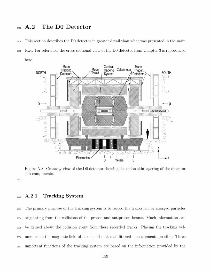
A.2 The D0 Detector2328

This section describes the D0 detector in greater detail than what was presented in the main2329

text. For reference, the cross-sectional view of the D0 detector from Chapter 3 is reproduced2330

here.

Figure A.8: Cutaway view of the D0 detector showing the onion skin layering of the detectorsub-components.

2331

A.2.1 Tracking System2332

The primary purpose of the tracking system is to record the tracks left by charged particles2333

originating from the collisions of the proton and antiproton beams. Much information can2334

be gained about the collision event from these recorded tracks. Placing the tracking vol-2335

ume inside the magnetic field of a solenoid makes additional measurements possible. Three2336

important functions of the tracking system are based on the information provided by the2337

159

recorded tracks. One such important function of the tracking system is vertexing. By ex-2338

trapolating tracks back towards the beam, the primary interaction vertex for the event can2339

be found with good precision. Secondary vertices caused by long-lived particles traveling a2340

short distance before decaying can also be detected. This plays a major role in detecting2341

long-lived b quark hadrons. Another important function is particle identification. Tracks2342

can be matched to particle showers seen in the calorimeters to help determine the particle2343

type. Determining the direction of curvature of the particle’s trajectory in the magnetic field2344

gives a measurement of the sign of its charge. The final function of the tracking system is2345

obtaining a momentum measurement of the particles traversing the detector. This is done2346

by measuring the curvature of the track in the magnetic field.2347

Many of these functions, particularly momentum measurements and vertexing, require2348

the tracking system to be the closest detector subsystem to the interaction point. Directly2349

outside the beam pipe, it occupies the radial space between 1.6 cm and 52 cm from the center2350

of the beam pipe and is 2.5 m in extent. Since the direction and position of these tracks is2351

important in reconstructing the collision event, care must be taken to minimize scattering of2352

the particles off active detector material and support structures. Particles passing through2353

the tracking system should not lose any appreciable amount of energy or be diverted from2354

their original path. The tracking system consists of low atomic number Z materials to2355

minimize the number of radiation lengths.2356

The tracking system consists of two detectors: the Silicon Microstrip Tracker and the2357

Central Fiber Tracker described in Section A.2.1.2 and Section A.2.1.3, respectively. Be-2358

cause the magnet system is an essential part of the tracking system it will be described in2359

Section A.2.1.1.2360

160

A.2.1.1 Magnets2361

The magnetic field which aids in tracking particles is provided by the combination of two2362

magnets: a solenoid and a toroid. The entire tracking system is inside the bore of the2363

solenoid magnet oriented parallel to the beam axis. The solenoid magnet along with the rest2364

of the detector (with the exception of some of the muon system) is inside the toroid magnet.2365

The central field of the solenoid is 2 T while the field in the toroid is 1.9 T. A projection2366

of the resulting magnetic field in the y-z plane is shown in Fig. A.9. The magnetic field is2367

symmetric about the x-z diagonal. The magnets’ polarity is periodically reversed and data2368

is taken in each of the four configurations.2369

Solenoid2370

The solenoid is a superconducting magnet that is 2.54 m long and 1.22 m in diameter.2371

The superconducting cables are made from eighteen Cu:NbTi strands stabilized in aluminum.2372

The cables are wound in two layers inside a supporting cylinder. The cables are cooled with2373

liquid helium and operate in the superconducting regime. A current of 4749 A through the2374

coils gives a central field of 2 T.2375

Toroid2376

The toroid is considered part of the muon system discussed in Section A.2.4 and also2377

serves as the return for some of the field lines of the solenoid. Unlike the solenoid, the toroid2378

operates in the classical regime. The magnet is made from iron windings around a steel2379

yoke and has three sections: two end toroids and one central toroid. The central toroid is a2380

square annulus about 1 m thick and 7.6 m long. It is wound with twenty coils of ten turns2381

each. The two end toroids are square with a 1.8 m square hole to accommodate the beam2382

161

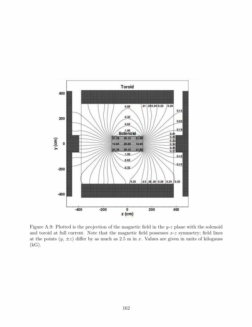
Figure A.9: Plotted is the projection of the magnetic field in the y-z plane with the solenoidand toroid at full current. Note that the magnetic field possesses x-z symmetry; field linesat the points (y, ±z) differ by as much as 2.5 m in x. Values are given in units of kilogauss(kG).

162

line. Each end toroid is wound with eight coils of eight turns each and is wired in series with2383

the central toroid. The current through the toroid is 1500 A giving a field inside the yoke of2384

1.8 T in the central toroid and 1.9 T in the end toroids.2385

A.2.1.2 Silicon Microstrip Tracker2386

The Silicon Microstrip Tracker (SMT) is a solid state semiconductor detector. Sensors are2387

made from bulk n-type2 silicon and are either single- or double-sided. Single-sided sensors2388

are made by implanting p-type3 silicon in strips on one side of the n-type bulk silicon.2389

Double-sided sensors are made by implanting strips of n-type silicon with a larger fraction2390

of donor impurities than the bulk material on the other side of single-sided sensors. Voltage2391

is applied across the strips such that the p-type implants sit at a negative voltage compared2392

to the n-type bulk or n-type strips. This creates a large region where there are no free2393

charge carriers as the holes (electrons) in the p-type (n-type) material are attracted to the2394

cathode (anode). This region is referred to as the depletion region and is the active area of2395

the detector. When a charged particle passes through the sensor it ionizes the material in2396

the depletion region creating electron-hole pairs. These migrate to the strips and the charge2397

is read out.2398

The detector is composed of many of these sensors arranged in barrels and disks. An2399

isometric view of the SMT is shown in Fig. A.10. The barrels provide a measurement of2400

the r-φ for the tracks in the central (small |η|) region of the detector. Disks measure the2401

r-z coordinate as well as the r-φ coordinate in the forward (high |η|) regions. There are six2402

barrels in total capped at the high |z| end by a disk composed of wedge detectors called2403

2N-type semiconductors have majority charge carriers (electrons) that are negative and are produced byadding impurities that donate electrons to the material lattice.

3P-type semiconductors have majority charge carriers (holes) that are positive and are produced by addingimpurities that accept electrons to the material lattice.

163

an F-disk. Each end of the barrel region is capped by three additional F-disks. One large2404

diameter disk, called an H-disk, is located in the far-forward regions. A separate system2405

called Layer 0 is installed inside the inner diameter of the barrels and disks.2406

Barrels2407

Each of the six barrels has four layers with each layer composed of two sublayers. The2408

barrel silicon module, called a ladder, consists of a 12 cm long sensor region and front-2409

end electronics necessary to read out the sensor on a beryllium substrate. Ladders in the2410

sublayers are arranged such that they provide an overlap in φ as in Fig. A.10. Each barrel

Figure A.10: An isometric view of the D0 SMT. Note that the two far-forward H-disks wereremoved to install Layer 0 (not shown).

2411

contains 72 ladders with sensors of varying widths. The second and fourth layer of all barrels2412

have ladders with double-sided silicon sensors. The p-side has strips oriented parallel to the2413

beam pipe with a strip-to-strip distance (pitch) of 50 µm. Strips on the n-side are oriented2414

at an angle of 2 with respect to the axial strips and have a pitch of 62.5 µm. The first and2415

third layers of the two outer barrels have single-sided ladders with a strip pitch of 50 µm2416

164

oriented parallel to the beam pipe. For the inner four barrels, the first and third layers have2417

double-sided ladders with a 90 stereo angle. The p-side strips are aligned parallel to the2418

beam pipe as in the single-sided devices while the n-side strips are perpendicular.2419

F-disks2420

There are 12 F-disks in all: one at the high |z| end of each of the six barrels and three at2421

each end of the barrel assembly. Each F-disk is made in 12 sections with one double-sided2422

sensor per section. The sensors are isosceles trapezoids with strips on either side aligned2423

with a long edge of the trapezoid, giving a 30 stereo angle. The sections are joined with2424

alternating p- and n-sides facing the center of the detector. The strip pitch for the p- and2425

n-sides are equal to those of the double-sided 2 barrel sensors. The active length of the2426

barrel/disk structure and the end F-disks is approximately 1066 mm.2427

H-disks2428

There are currently two H-disks in the D0 detector, though there were four at the begin-2429

ning of Run II. They are located at z ≈ ±100 cm. Twenty-four trapezoidal sensors comprise2430

each H-disk. Each sensor is formed by gluing two single-sided sensors back-to-back. Like the2431

F-disks, strips are aligned with a long edge of the trapezoid, giving an effective stereo angle2432

of 15. The strip pitch for these detectors is 40 µm.2433

Layer 02434

Layer 0 was installed along with a new beryllium beam pipe in 2006. It resides in the space2435

between the beam pipe and the first layers of the barrels. The whole device is approximately2436

1660 mm long with the sensors covering z ≤ |380| mm. There are 48 single-sided sensors in2437

165

all with strip pitches of 71 µm and 81 µm. They are arranged on a hexagonal carbon fiber2438

support tube with a row of eight sensors on each face. Rows alternate between 16.1 mm and2439

17.6 mm from the beam axis. The 71(81) µm strip pitch sensors are located 16.1(17.6) mm2440

from the beam.2441

A.2.1.3 Central Fiber Tracker2442

The Central Fiber Tracker (CFT) is a scintillating fiber detector. The passage of charged2443

particles through the fibers produces photons from ionization and excitation events. Because2444

the number of photons produced in scintillating fiber for an ionization/excitation event is2445

small, it is important that the device detecting these photons is extremely sensitive. We2446

use visual light photon counters (VLPCs) which produce an electrical signal in response2447

to photons and are capable of detecting single photons. Fibers were made by extruding2448

polystyrene doped with two fluorescent dyes. The primary fluorescent dye (about 1% by2449

weight) is rapidly excited by the neighboring excited polystyrene through a non-radiative2450

near-field interaction. The primary fluorescent rapidly relaxes and emits a short wavelength2451

(≈ 340 nm) photon. Because this photon does not travel far in polystyrene, the second dye,2452

a wavelength-shifter, is necessary. The second dye (present at about 1500 ppm) absorbs2453

this photon and re-emits it at ≈ 530 nm, which is transmitted well by polystyrene. With2454

two claddings of decreasing index of refraction the attenuation length in these scintillating2455

fibers is approximately 5 m. Once out of the active volume of the CFT, the light travels in2456

light-shielded clear fibers which are chemically similar to the scintillating fibers all the way2457

to the VLPCs at the bottom of the detector.2458

166

Fiber Arrangement2459

The scintillating fibers in the CFT are 835 µm in diameter and are 1.66 m or 2.52 m2460

in length. They are grouped into ribbons of 256 fibers each in two rows of 128. The fiber2461

spacing ranges from 928 µm to 990 µm and depends on the radius at which the fibers are2462

located. The second row of fibers is offset from the first by half this distance. These ribbons2463

are bonded to the outside of carbon fiber support cylinders in two layers: an axial layer and2464

a stereo layer. In the axial layer the fibers are oriented parallel to the beam axis. The stereo2465

layer has fibers oriented at a ±3 angle with respect to the axial layer. The sign of the angle2466

alternates between cylinders. There are eight cylinders total occupying the radial space from2467

20 cm to 52 cm.2468

A.2.2 Preshower Detectors2469

Directly outside the solenoid before the calorimeter are the preshower detectors. They can be2470

considered part of both the tracking system and the calorimetry; they mark the beginning of2471

electromagnetic showering and are used to match tracks to showers seen in the calorimeter.2472

Like the CFT, the preshower detectors use scintillation light to detect the passage of charged2473

particles. Instead of single fibers the preshower detectors use polystyrene strips with a2474

triangular cross section. The strips are doped with fluorescent dye and a wavelength-shifting2475

fiber is placed in the center. The light is collected by the center fiber and transferred2476

to VLPCs for read-out via clear fiber. There are three preshower detectors: the Central2477

Preshower detector (CPS) and two Forward Preshower detectors (FPS). All three use the2478

same type of scintillating strips but the strips are arranged differently for the CPS and FPS.2479

167

CPS2480

The CPS sits between the solenoid and the calorimeter. Directly outside the solenoid2481

is a lead radiator covered with steel. This radiator and the solenoid provide about two2482

radiation lengths to particles with normal incidence. At larger angles this increases to about2483

four radiation lengths. Scintillator strips in the CPS are nested together to form single2484

layers that are approximately 7 mm tall, slightly taller than the strips themselves. The CPS2485

consists of three such layers of scintillator: one axial layer and two stereo layers with angles2486

of ≈ ±24.2487

FPS2488

There are two FPS detectors, one on either end of the D0 detector. They are mounted on2489

the end calorimeter cryostats (see Section A.2.3). Scintillator strips in the FPS are nested2490

together such that a layer of scintillator is about as tall as a strip: about 5 mm. There are2491

four super-layers separated in z in each FPS detector. Each super-layer consists of eight2492

active φ = 22.5 modules separated by eight inactive regions. The second and fourth super-2493

layers are rotated by 22.5 with respect to the first and third super-layers, creating two active2494

effective layers in each 22.5 wedge. Each layer consists of two sublayers of scintillator strips2495

with a 22.5 stereo angle between them. The inner layer is shorter than the outer layer and2496

mainly detects minimally ionizing particles. Between the inner and outer layer is a short2497

piece of lead/steel absorber which adds two radiation lengths in the path of the particles2498

producing electromagnetic showers in the outer layer. The solenoid provides up to three2499

radiation lengths for particles traveling in the outer area of the outer layer where there is no2500

absorber.2501

168

A.2.3 Calorimeters2502

The primary purpose of the calorimeter is to make a measurement of the energy of particles2503

produced in the D0 detector. Unlike the tracking system which is designed to measure the2504

passage of particles with minimal disturbance, the calorimeter is designed to stop particles2505

completely. In this way particles make a complete deposit of their energy. The D0 detec-2506

tor uses a sampling calorimeter that has alternating layers of absorber and active material.2507

Particles traveling through the absorber create showers of secondary particles that are either2508

electromagnetic or hadronic in nature as described in Section 1.4.3.1. These secondary parti-2509

cles ionize the active material and the charge is collected and measured. The D0 calorimeter2510

is a compensating combined electromagnetic (EM) and hadronic calorimeter; it has an equal2511

response to electromagnetic and hadronic particles with the same energy. Because EM and2512

hadronic shower generation is governed by two different length scales – the radiation length2513

(X0) and the nuclear interaction length (λA) – the calorimeter has varying absorber thick-2514

nesses and materials to capture both types of showers. In high Z materials X0 is much2515

smaller than λA so EM showers occur closer to the interaction region than hadronic show-2516

ers. The D0 calorimeter has three showering layers: the EM layer, the fine hadronic layer,2517

and the coarse hadronic layer. The active material in the D0 calorimeter is liquid argon.2518

For accessibility, the calorimeter is divided into three separate cryostats, a central cryostat2519

and two end cryostats. Depending on the layer and cryostat the absorber is either depleted2520

uranium, a uranium-niobium alloy, copper, or steel. A typical calorimeter cell is shown in2521

Fig. A.11. Sensor pads interleaved between sheets of absorber are patterned for segmented2522

readout. Cells whose centers lie at the same η and φ are ganged together in depth to create2523

readout towers as shown in Fig. A.12.2524

169

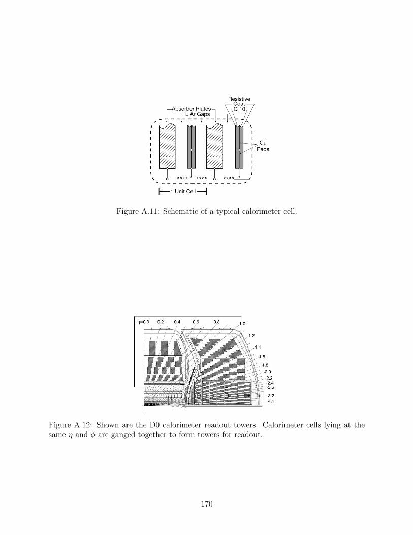
Figure A.11: Schematic of a typical calorimeter cell.

Figure A.12: Shown are the D0 calorimeter readout towers. Calorimeter cells lying at thesame η and φ are ganged together to form towers for readout.

170

Central Calorimeter2525

The central calorimeter (CC) covers the region |η| . 1. The EM section is made from2526

3 mm-thick absorber plates of nearly pure depleted uranium. It has four separate depth2527

layers, or gangings, that are 1.4, 2.0, 6.8, and 9.8 X0 thick. The total number of radiation2528

lengths from material between the calorimeter and the interaction region is about four at2529

η = 0. The fine hadronic section is made from 6 mm-thick plates of a uranium-niobium2530

alloy. It has three gangings that are 1.3, 1.0, and 0.76 λA thick. There is only one coarse2531

hadronic layer made from 46.5 mm-thick plates of copper that is 3.2 λA thick.2532

End Calorimeters2533

The end calorimeters (EC) extend the coverage of the calorimeter to |η| . 4. The material2534

between the interaction region and the first active gap in the EC provides approximately2535

4.4 X0 of material at η = 2. Like the CC, the EC has four depth layers in the EM section2536

that are approximately 1.6, 2.6, 7.9, and 9.3 X0 thick. The EM section is a disk made from2537

plates of nearly pure depleted uranium 4 mm thick. The hadronic sections of the EC are2538

divided into three regions from the beam line: the inner hadronic, middle hadronic, and outer2539

hadronic regions. The inner and middle hadronic regions have both fine and coarse hadronic2540

sections. Fine hadronic sections are made from 6 mm-thick uranium-niobium plates and have2541

four gangings 1.1(0.9) λAthick in the inner (middle) hadronic sections. There is only one2542

depth layer for the inner (middle) coarse hadronic section that is made from 46.5 mm-thick2543

steel plates with a total thickness of 4.1(4.4) λA. The outer hadronic region has only one2544

coarse hadronic ganging made from the same steel plates with a total maximum thickness of2545

6.0 λA. These plates are inclined at an angle of approximately 60 with respect to the beam2546

axis to avoid cracks.2547

171

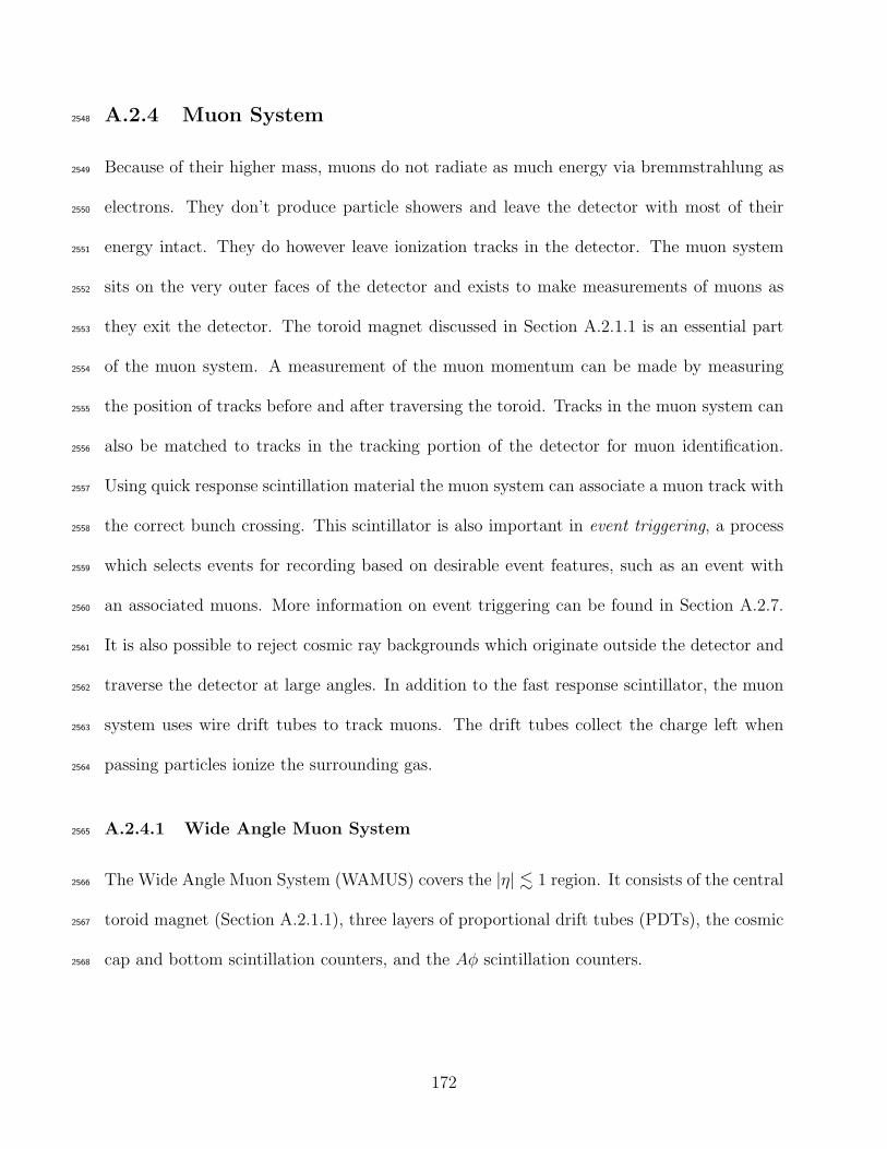
A.2.4 Muon System2548

Because of their higher mass, muons do not radiate as much energy via bremmstrahlung as2549

electrons. They don’t produce particle showers and leave the detector with most of their2550

energy intact. They do however leave ionization tracks in the detector. The muon system2551

sits on the very outer faces of the detector and exists to make measurements of muons as2552

they exit the detector. The toroid magnet discussed in Section A.2.1.1 is an essential part2553

of the muon system. A measurement of the muon momentum can be made by measuring2554

the position of tracks before and after traversing the toroid. Tracks in the muon system can2555

also be matched to tracks in the tracking portion of the detector for muon identification.2556

Using quick response scintillation material the muon system can associate a muon track with2557

the correct bunch crossing. This scintillator is also important in event triggering, a process2558

which selects events for recording based on desirable event features, such as an event with2559

an associated muons. More information on event triggering can be found in Section A.2.7.2560

It is also possible to reject cosmic ray backgrounds which originate outside the detector and2561

traverse the detector at large angles. In addition to the fast response scintillator, the muon2562

system uses wire drift tubes to track muons. The drift tubes collect the charge left when2563

passing particles ionize the surrounding gas.2564

A.2.4.1 Wide Angle Muon System2565

The Wide Angle Muon System (WAMUS) covers the |η| . 1 region. It consists of the central2566

toroid magnet (Section A.2.1.1), three layers of proportional drift tubes (PDTs), the cosmic2567

cap and bottom scintillation counters, and the Aφ scintillation counters.2568

172

Proportional Drift Tubes2569

There are three layers of PDTs in WAMUS denoted A, B, and C. The A-layer resides2570

between the calorimeter and the central toroid magnet while the B- and C-layers lie outside2571

the central toroid. Each layer consists of either three or four stacks of PDTs. Each 10.1 cm2572

PDT cell is made from a long rectangular aluminum tube with an anode wire in the center2573

and a cathode pad above and below the anode wire. The tube is filled with 84% argon and2574

8% CH4/CF4 that gives a maximum electron drift time of 500 ns. Two anode wires are2575

ganged together and are read out at one end of each cell. Position information along the2576

PDT is gathered from the timing difference between the signal at the end of the struck wire2577

and the signal at the end of its partner’s wire. The position resolution using this method2578

can be anywhere from 10 cm-50 cm depending on where the hit occurred. Information about2579

the amount of charge deposited on the cathode pads can bring the resolution down to about2580

5 mm. As can be seen in the exploded view of the D0 muon wire chambers in Fig. A.13, the2581

PDT coverage on the bottom is sparse due to the calorimeter supports. Still, approximately2582

55% of the central region is covered by three layers of PDTs and close to 90% of the region2583

is covered by at least two layers of PDTs.2584

Cosmic Cap and Bottom2585

The cosmic cap and bottom scintillation counters cover the outer layer of the central2586

muon PDTs. The cosmic cap refers to the counters covering the top and sides of the central2587

muon C-layer PDTs while the cosmic bottom refers to counters covering the bottom B- and2588

C-layer central muon PDTs. Both provide fast timing information that is used to associate a2589

hit in a PDT with the appropriate bunch crossing and to reject the cosmic ray background.2590

There are 240 cosmic cap scintillation counters. Each counter is made from 0.5 in-thick2591

173

plastic scintillator 25 in wide and 81.5 in-113 in long. They are oriented with their length2592

along φ and their width along z. Light from charged particle interactions is gathered by2593

wavelength shifting fibers that are glued into grooves along the length of the scintillator2594

from each end to just past the center. Fibers are collected in the center into two bundles and2595

the light is detected by two photomultiplier tubes (PMTs) mounted directly on the counter.2596

There are 132 counters in the cosmic bottom on the outside of the B and C PDT layers.2597

Refer to Fig. A.14 for the placement of the counters. In contrast to the cosmic cap counters,2598

the cosmic bottom counters are placed with their width along φ and their length along z.2599

There are two types of counters employed in the cosmic bottom; both are similar in design to2600

the cosmic cap counters. Forty-eight counters in the center bottom B-layer are identical to2601

the cosmic cap counters with minor improvements in edge fiber placement. There are sixteen2602

total counters located on the bottom sides of the B-layer PDTs. The remaining 68 counters2603

on the bottom B- and C-layer PDTs have fewer total fibers that are placed in vertical rather2604

than horizontal grooves like those in the cosmic cap. The light yield in this arrangement is2605

similar to that in the cosmic cap. Like the cosmic cap, light is detected by PMTs mounted2606

directly on the counter.2607

Aφ Scintillation Counters2608

In addition to the scintillator on the outer layers of central muon PDTs there is another2609

layer of scintillator on the outside of the A-layer PDTs generally referred to as the Aφ2610

scintillation counters. These counters are used for identifying and triggering on muons,2611

rejecting backscattering from the forward direction, and providing a time stamp on low pT2612

muons that may not reach the cosmic cap and bottom counters. The counters are made from2613

scintillator plastic with wavelength shifting fibers embedded in vertical grooves in a manner2614

174

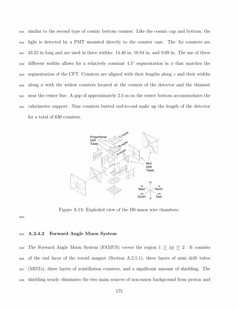
similar to the second type of cosmic bottom counter. Like the cosmic cap and bottom, the2615

light is detected by a PMT mounted directly to the counter case. The Aφ counters are2616

33.25 in long and are used in three widths: 14.46 in, 10.84 in, and 9.09 in. The use of three2617

different widths allows for a relatively constant 4.5 segmentation in φ that matches the2618

segmentation of the CFT. Counters are aligned with their lengths along z and their widths2619

along φ with the widest counters located at the corners of the detector and the thinnest2620

near the center line. A gap of approximately 2.5 m on the center bottom accommodates the2621

calorimeter support. Nine counters butted end-to-end make up the length of the detector2622

for a total of 630 counters.

Figure A.13: Exploded view of the D0 muon wire chambers.

2623

A.2.4.2 Forward Angle Muon System2624

The Forward Angle Muon System (FAMUS) covers the region 1 . |η| . 2. It consists2625

of the end faces of the toroid magnet (Section A.2.1.1), three layers of mini drift tubes2626

(MDTs), three layers of scintillation counters, and a significant amount of shielding. The2627

shielding nearly eliminates the two main sources of non-muon background from proton and2628

175

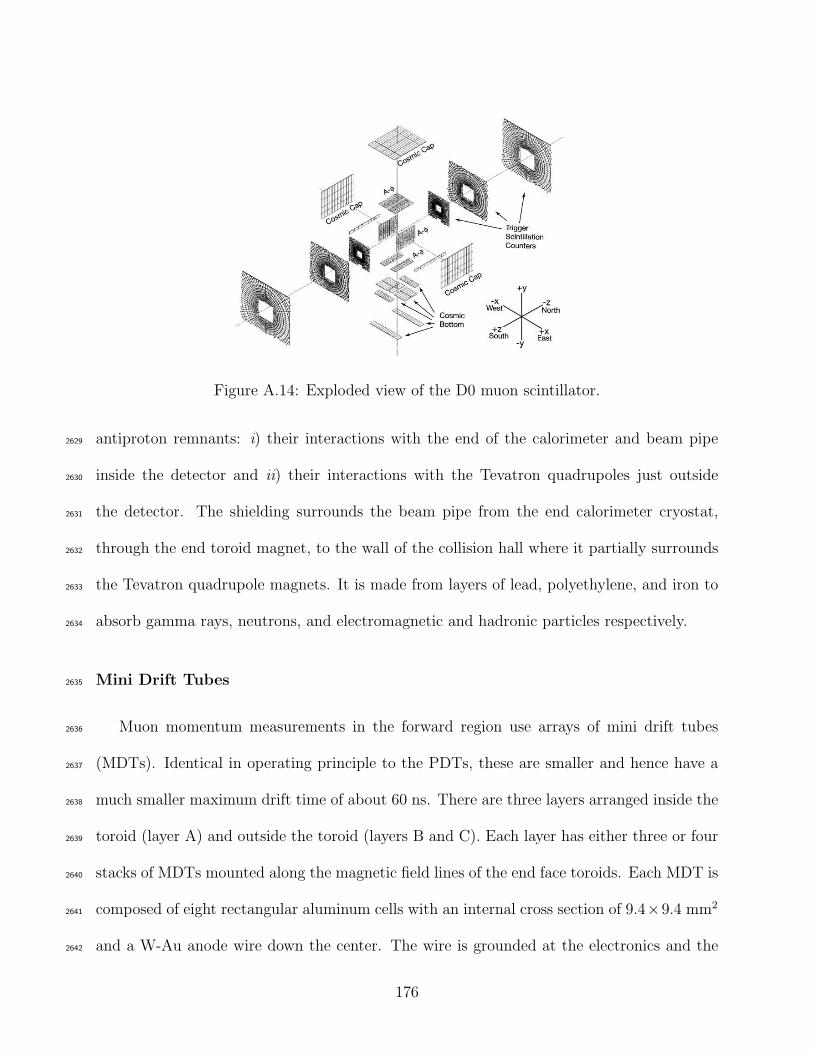
Figure A.14: Exploded view of the D0 muon scintillator.

antiproton remnants: i) their interactions with the end of the calorimeter and beam pipe2629

inside the detector and ii) their interactions with the Tevatron quadrupoles just outside2630

the detector. The shielding surrounds the beam pipe from the end calorimeter cryostat,2631

through the end toroid magnet, to the wall of the collision hall where it partially surrounds2632

the Tevatron quadrupole magnets. It is made from layers of lead, polyethylene, and iron to2633

absorb gamma rays, neutrons, and electromagnetic and hadronic particles respectively.2634

Mini Drift Tubes2635

Muon momentum measurements in the forward region use arrays of mini drift tubes2636

(MDTs). Identical in operating principle to the PDTs, these are smaller and hence have a2637

much smaller maximum drift time of about 60 ns. There are three layers arranged inside the2638

toroid (layer A) and outside the toroid (layers B and C). Each layer has either three or four2639

stacks of MDTs mounted along the magnetic field lines of the end face toroids. Each MDT is2640

composed of eight rectangular aluminum cells with an internal cross section of 9.4×9.4 mm22641

and a W-Au anode wire down the center. The wire is grounded at the electronics and the2642

176

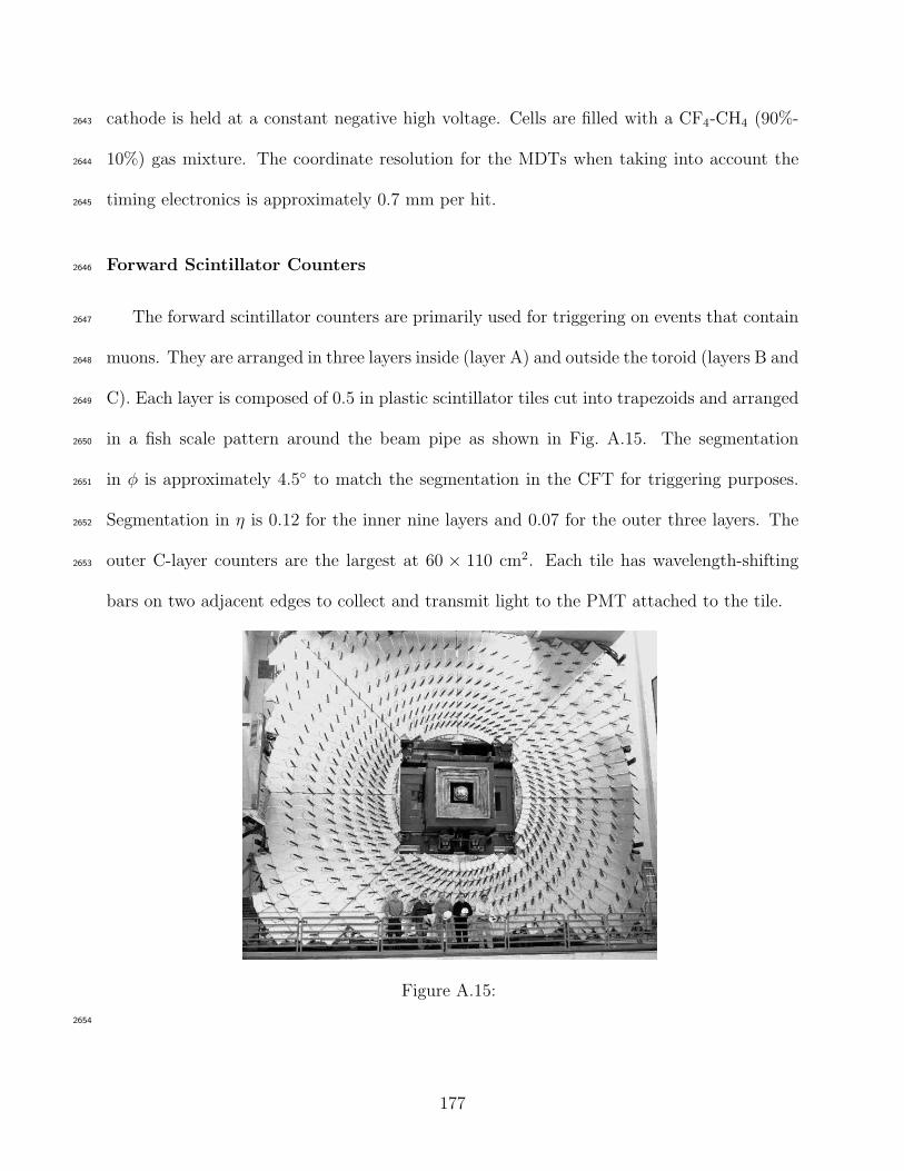
cathode is held at a constant negative high voltage. Cells are filled with a CF4-CH4 (90%-2643

10%) gas mixture. The coordinate resolution for the MDTs when taking into account the2644

timing electronics is approximately 0.7 mm per hit.2645

Forward Scintillator Counters2646

The forward scintillator counters are primarily used for triggering on events that contain2647

muons. They are arranged in three layers inside (layer A) and outside the toroid (layers B and2648

C). Each layer is composed of 0.5 in plastic scintillator tiles cut into trapezoids and arranged2649

in a fish scale pattern around the beam pipe as shown in Fig. A.15. The segmentation2650

in φ is approximately 4.5 to match the segmentation in the CFT for triggering purposes.2651

Segmentation in η is 0.12 for the inner nine layers and 0.07 for the outer three layers. The2652

outer C-layer counters are the largest at 60 × 110 cm2. Each tile has wavelength-shifting2653

bars on two adjacent edges to collect and transmit light to the PMT attached to the tile.

Figure A.15:

2654

177

A.2.5 Forward Proton Detector2655

A subdetector, called the Forward Proton Detector (FPD), designed to measure scattered2656

protons and antiprotons that do not impinge on the main detector is located on either side of2657

the detector inside the Tevatron tunnel. It is primarily used to tag diffractive events where2658

one or both incident protons survive the interaction intact4 and are scattered at very small2659

angles with respect to the beam.2660

The FPD is a momentum spectrometer that uses magnets in the accelerator lattice and2661

position detectors which can be moved very close to the beam. There are nine independent2662

spectrometers: one on the outgoing antiproton side of the D0 detector downstream from2663

the bending dipole magnet and four on each side of the D0 detector downstream from the2664

low β quadrupoles. There are two horizontal (in and out) and two vertical (up and down)2665

spectrometers to either side of the D0 detector. The spectrometer downstream from the2666

bending dipole is to the inside of the bend. Each spectrometer has an upstream and a2667

downstream position detector. The position detectors are housed in movable stainless steel2668

containers called Roman pots which allow them to operate outside the ultra-high vacuum2669

of the beam pipe and be retracted during suboptimal beam conditions. Roman pots are2670

grouped into castles: four castles with four Roman pots each serving the upstream and2671

downstream position detectors of the eight spectrometers nearest the D0 detector and two2672

castles with one Roman pot each serving the spectrometer downstream from the bending2673

dipole.2674

The position detectors are made from six stacks of scintillating fiber ribbons arranged2675

with the edges of the ribbons in the plane perpendicular to the beam. Stacks are oriented at2676

4Contrary to elastic scattering, additional particles are produced in the scattering event even in the casewhere both protons are intact.

178

angles of ±45 and 90 with respect to the bottom of the detector. There are two stacks in2677

each orientation that are offset by 2/3 of the fiber width. Scattered protons and antiprotons2678

travel through a thin steel window and impinge on the scintillator. Fibers are read out by2679

multi-anode photomultiplier tubes and integrated into the CFT electronics. Between the 902680

and −45 layers is a solid piece of scintillating plastic read out by a fast photomultiplier2681

tube that is used for triggering purposes (See Section A.2.7).2682

A.2.6 Luminosity Monitor2683

Measuring the instantaneous luminosity being provided to D0 by the Tevatron is an im-2684

portant process both for online operation and off-line data analysis. The instantaneous2685

luminosity dictates the trigger set used at a given time during operation and therefore de-2686

termines the physics processes being recorded for later analysis. Off-line analyses require2687

an accurate luminosity measurement for proper event yield predictions of specific processes.2688

The D0 subdetector responsible for measuring the instantaneous luminosity is the Luminos-2689

ity Monitor (LM). Additionally, the LM provides a fast measurement of the z coordinate of2690

the interaction vertex and a measurement of the beam halo.2691

These measurements are done by detecting inelastic proton-antiproton collisions through2692

scintillation light. Two arrays of plastic scintillation counters located at z = ±140 cm2693

comprise the LM. Each array contains 24 counters divided into two enclosures attached to2694

the spherical head of the end calorimeters. At 15 cm long, they occupy the radial space2695

between the beam pipe and the FPS detector over the pseudorapidity range 2.7 < |η| < 4.4.2696

Their location in the forward region close to the interaction point necessitates the use of2697

radiation-hard PMTs for readout.2698

Signals from each array are collected and a timing pulse is created for each array. The2699

179

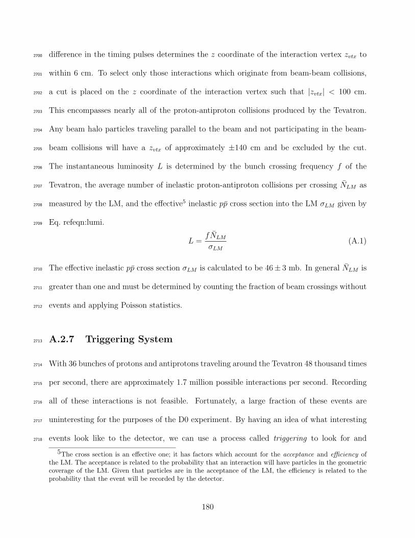
difference in the timing pulses determines the z coordinate of the interaction vertex zvtx to2700

within 6 cm. To select only those interactions which originate from beam-beam collisions,2701

a cut is placed on the z coordinate of the interaction vertex such that |zvtx| < 100 cm.2702

This encompasses nearly all of the proton-antiproton collisions produced by the Tevatron.2703

Any beam halo particles traveling parallel to the beam and not participating in the beam-2704

beam collisions will have a zvtx of approximately ±140 cm and be excluded by the cut.2705

The instantaneous luminosity L is determined by the bunch crossing frequency f of the2706

Tevatron, the average number of inelastic proton-antiproton collisions per crossing NLM as2707

measured by the LM, and the effective5 inelastic pp cross section into the LM σLM given by2708

Eq. refeqn:lumi.2709

L =fNLM

σLM

(A.1)

The effective inelastic pp cross section σLM is calculated to be 46± 3 mb. In general NLM is2710

greater than one and must be determined by counting the fraction of beam crossings without2711

events and applying Poisson statistics.2712

A.2.7 Triggering System2713

With 36 bunches of protons and antiprotons traveling around the Tevatron 48 thousand times2714

per second, there are approximately 1.7 million possible interactions per second. Recording2715

all of these interactions is not feasible. Fortunately, a large fraction of these events are2716

uninteresting for the purposes of the D0 experiment. By having an idea of what interesting2717

events look like to the detector, we can use a process called triggering to look for and2718

5The cross section is an effective one; it has factors which account for the acceptance and efficiency ofthe LM. The acceptance is related to the probability that an interaction will have particles in the geometriccoverage of the LM. Given that particles are in the acceptance of the LM, the efficiency is related to theprobability that the event will be recorded by the detector.

180

record only the events we find interesting. D0 uses a three-tiered triggering system based2719

in both hardware and software to accomplish this. The levels are designed to act as a2720

filtering system with each step increasing in complexity. The Level 1 (L1) trigger consists of2721

hardware elements with an accept rate of approximately 2 kHz. Events that pass are sent to2722

the Level 2 (L2) system which consists of hardware and microprocessors associated with each2723

subdetector and a global processor that makes trigger decisions not only based on individual2724

physics objects but object correlations as well. The accept rate of L2 is approximately 1 kHz.2725

If an event is passed by L2 it is sent to the farm of about 250 computer nodes that make up2726

Level 3 (L3). Level 3 passes events at a rate of about 50 Hz. Those events are recorded for2727

later offline reconstruction.2728

A.2.7.1 Level 12729

Level 1 is implemented in hardware devices which originate in four detector subsystems:2730

the scintillating fiber tracking system, the calorimeter, the muon system, and the forward2731

proton detector. Every event is examined and each subsystem submits event information to2732

the trigger framework (TFW). The TFW constructs physics triggers from the triggers con-2733

structed by the L1 systems using AND/OR logical operators. In addition to the construction2734

of physics triggers the TFW manages communication with the front-end electronics and the2735

trigger control computer, applies prescaling to triggers, and coordinates readout upon a L22736

accept. The logical OR of the physics triggers is what determines whether the event is2737

selected for additional processing in Level 2.2738

181

L1 Tracking2739

The scintillating fiber systems which participate in the Level 1 trigger decision are the2740

FPS and CFT/CPS axial systems, collectively referred to as the Central Track Trigger2741

(L1CTT). By design these systems provide triggers for charged particles with a transverse2742

momentum pT greater than 1.5 GeV. Finding tracks, finding energy clusters originating in2743

the preshower detectors, and matching tracks to clusters are the main functions of the2744

scintillating fiber systems in L1. Significant processing resources are reserved for finding and2745

triggering on isolated charged particle tracks. In addition, lists of tracks are sent to the L12746

muon system to be used as seeds.2747

L1 Calorimeter2748

The calorimeter groups readout towers two by two in η and φ into trigger towers. Trans-2749

verse energy ET thresholds are set for the sum total of all trigger towers and for each trigger2750

tower individually. In addition, thresholds can be defined for the total unbalanced or “miss-2751

ing” transverse energy 6ET . The partial sums necessary for the calculation can be used to2752

trigger on jets which are much larger than the trigger towers.2753

L1 Muon2754

The Level 1 muon system looks for hit patterns consistent with the passage of a muon2755

using the muon scintillator and wire chambers and the seed tracks from the L1CTT system.2756

Triggers are formed in the scintillator by 1) matching L1CTT tracks to hits in either the2757

A-layer or the A- and B-layer and 2) requiring hits in either the A-layer or the A- and B-2758

layer without a matched track. Additionally, hits in the muon wire chambers are used to2759

confirm scintillator hits in each layer. These confirmed hits are used to form triggers 3) in2760

182

either the A-layer or the A- and B-layer scintillator. I swear to gods there are way too many2761

’scintillators’...2762

L1 FPD2763

The Forward Proton Detector also takes part in the Level 1 trigger. It selects events2764

in which beam particles leave the interaction region intact and hit one or more FPD spec-2765

trometers. We create a pixel grid from the stacks of scintillating ribbon in the position2766

detectors and compare pixel hits to detector pixel hit patterns stored in hardware. Timing2767

information is obtained from the trigger scintillator using fast photomultiplier tubes. The2768

FPD trigger system uses this timing information to look for coincidences between hit signals2769

of both position detectors for any of the nine spectrometers signaling the passage of an intact2770

beam particle. Coincidences between spectrometers on either side of the interaction region2771

are indicative of an event where both beam particles leave the interaction region intact.2772

A.2.7.2 Level 22773

Following a Level 1 accept from the TFW, the event begins processing at L2. Level 2 consists2774

of a detector-specific preprocessing stage and a global processing stage. The preprocessing2775

stage collects information from the L1 trigger system and the detector front-ends to form2776

physics objects. At the global level, data from different parts of the detector can be com-2777

bined to form higher-quality physics objects than those available at the preprocessing stage.2778

In addition, correlations between objects across the whole detector can be examined. All2779

detector subsystems participating in Level 1 also participate in Level 2 with the exception2780

of the Forward Proton Detector. Also participating in L2 is the Silicon Microstrip Tracker.2781

The finer spatial resolution of the SMT with respect to the CFT allows for a more precise2782

183

track reconstruction and an improved momentum measurement. The L2 global processing2783

stage runs algorithms on the data received from the preprocessors based on what triggers2784

fired at Level 1. The L2 global decision is returned to the TFW.2785

A.2.7.3 Level 32786

Events which pass Level 2 are sent to the Level 3 trigger. Level 3 is a fully programmable2787

software trigger which has access to the full detector information. It performs a limited2788

reconstruction of the full event and makes its decision based on complete physics objects2789

and their relationships. The software resides on about 250 commercial computers running2790

the Linux operating system. Event fragments from different parts of the detector are routed2791

to a single L3 node where the event is built and made available to L3 processes. Events2792

selected by L3 are destined for storage on tape and full offline reconstruction.2793

184

Appendix B2794

Additional Distributions2795

This appendix contains additional plots and tables not included in the main text.2796

B.1 Additional V X Distributions2797

Plots of the invariant (transverse) mass are included for all V H analyses for each b-tagging2798

channel and purity region. The high-purity plots for the WH analysis are reproduced here2799

for comparison.2800

185

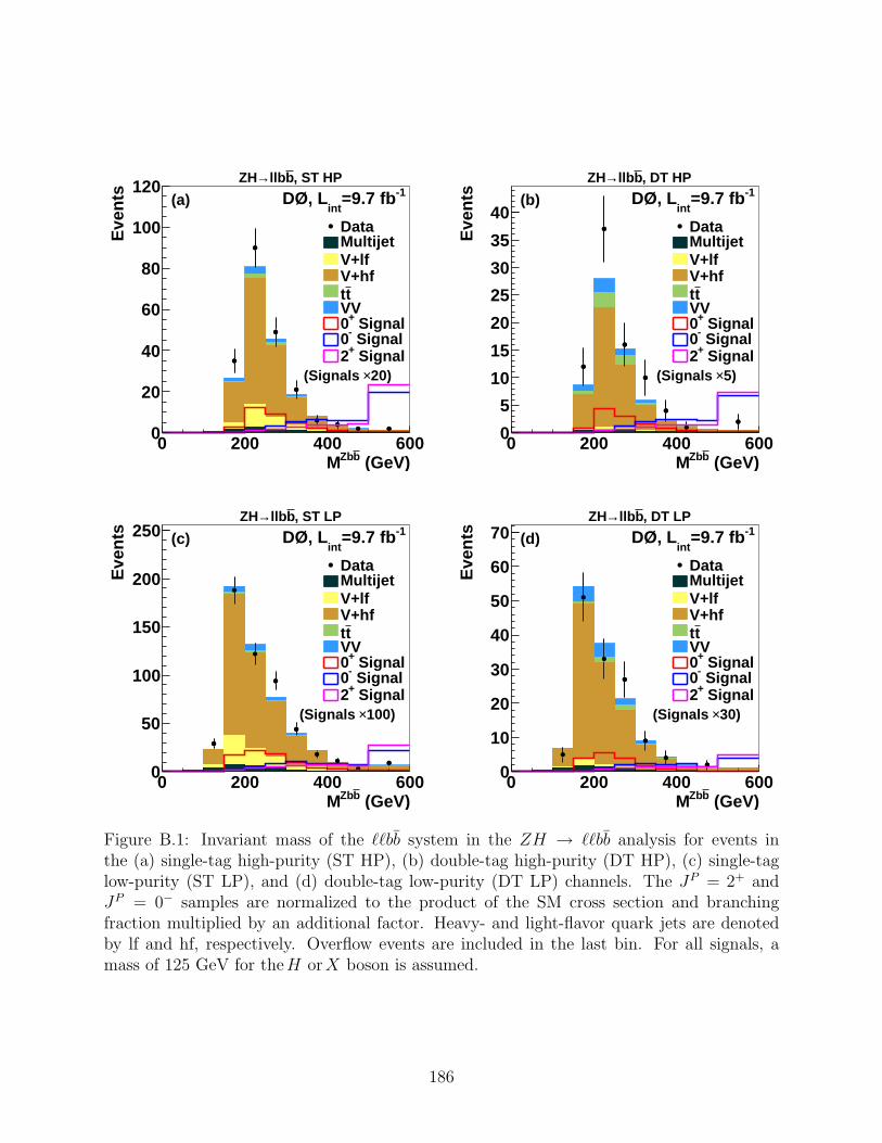
(GeV)bZbM0 200 400 600

Eve

nts

0

20

40

60

80

100

120 -1=9.7 fbint

DØ, L

20)×(Signals

DataMultijetV+lfV+hftt

VV Signal+0 Signal-0 Signal+2

, ST HPbllb→ZH

(a)

(GeV)bZbM0 200 400 600

Eve

nts

0

5

10

15

20

25

30

35

40-1=9.7 fb

intDØ, L

5)×(Signals

DataMultijetV+lfV+hftt

VV Signal+0 Signal-0 Signal+2

, DT HPbllb→ZH

(b)

(GeV)bZbM0 200 400 600

Eve

nts

0

50

100

150

200

250 -1=9.7 fbint

DØ, L

100)×(Signals

DataMultijetV+lfV+hftt

VV Signal+0 Signal-0 Signal+2

, ST LPbllb→ZH

(c)

(GeV)bZbM0 200 400 600

Eve

nts

0

10

20

30

40

50

60

70 -1=9.7 fbint

DØ, L

30)×(Signals

DataMultijetV+lfV+hftt

VV Signal+0 Signal-0 Signal+2

, DT LPbllb→ZH

(d)

Figure B.1: Invariant mass of the ℓℓbb system in the ZH → ℓℓbb analysis for events inthe (a) single-tag high-purity (ST HP), (b) double-tag high-purity (DT HP), (c) single-taglow-purity (ST LP), and (d) double-tag low-purity (DT LP) channels. The JP = 2+ andJP = 0− samples are normalized to the product of the SM cross section and branchingfraction multiplied by an additional factor. Heavy- and light-flavor quark jets are denotedby lf and hf, respectively. Overflow events are included in the last bin. For all signals, amass of 125 GeV for theH orX boson is assumed.

186

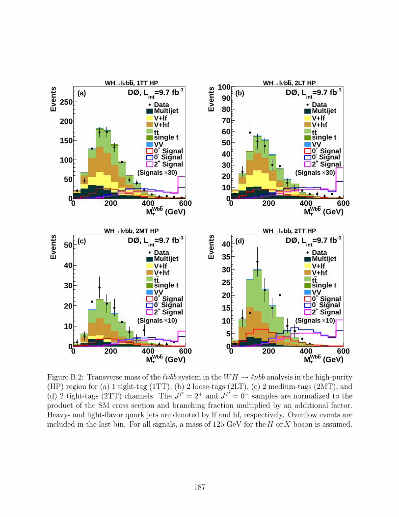
(GeV)bWbTM

0 200 400 600

Eve

nts

0

50

100

150

200

250

-1=9.7 fbint

DØ, L

30)×(Signals

DataMultijetV+lfV+hftt

single tVV

Signal+0 Signal-0 Signal+2

, 1TT HPbbνl→WH

(a)

(GeV)bWbTM

0 200 400 600E

vent

s

0102030405060708090

100 -1=9.7 fbint

DØ, L

30)×(Signals

DataMultijetV+lfV+hftt

single tVV

Signal+0 Signal-0 Signal+2

, 2LT HPbbνl→WH

(b)

(GeV)bWbTM

0 200 400 600

Eve

nts

0

10

20

30

40

50-1=9.7 fb

intDØ, L

10)×(Signals

DataMultijetV+lfV+hftt

single tVV

Signal+0 Signal-0 Signal+2

, 2MT HPbbνl→WH

(c)

(GeV)bWbTM

0 200 400 600

Eve

nts

0

5

10

15

20

25

30

35

40-1=9.7 fb

intDØ, L

10)×(Signals

DataMultijetV+lfV+hftt

single tVV

Signal+0 Signal-0 Signal+2

, 2TT HPbbνl→WH

(d)

Figure B.2: Transverse mass of the ℓνbb system in the WH → ℓνbb analysis in the high-purity(HP) region for (a) 1 tight-tag (1TT), (b) 2 loose-tags (2LT), (c) 2 medium-tags (2MT), and(d) 2 tight-tags (2TT) channels. The JP = 2+ and JP = 0− samples are normalized to theproduct of the SM cross section and branching fraction multiplied by an additional factor.Heavy- and light-flavor quark jets are denoted by lf and hf, respectively. Overflow events areincluded in the last bin. For all signals, a mass of 125 GeV for theH orX boson is assumed.

187

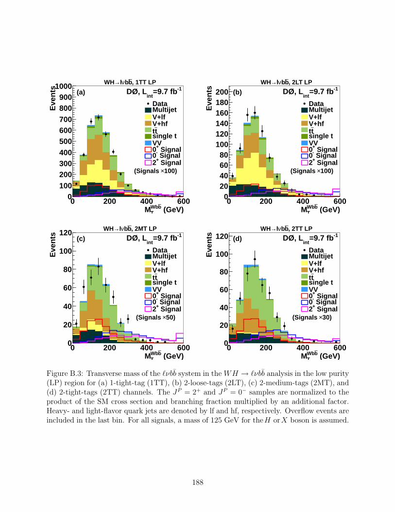
(GeV)bWbTM

0 200 400 600

Eve

nts

0100200300400500600700800900

1000 -1=9.7 fbint

DØ, L

100)×(Signals

DataMultijetV+lfV+hftt

single tVV

Signal+0 Signal-0 Signal+2

, 1TT LPbbνl→WH

(a)

(GeV)bWbTM

0 200 400 600E

vent

s

020406080

100120140160180200 -1=9.7 fb

intDØ, L

100)×(Signals

DataMultijetV+lfV+hftt

single tVV

Signal+0 Signal-0 Signal+2

, 2LT LPbbνl→WH

(b)

(GeV)bWbTM

0 200 400 600

Eve

nts

0

20

40

60

80

100

120 -1=9.7 fbint

DØ, L

50)×(Signals

DataMultijetV+lfV+hftt

single tVV

Signal+0 Signal-0 Signal+2

, 2MT LPbbνl→WH

(c)

(GeV)bWbTM

0 200 400 600

Eve

nts

0

20

40

60

80

100

120 -1=9.7 fbint

DØ, L

30)×(Signals

DataMultijetV+lfV+hftt

single tVV

Signal+0 Signal-0 Signal+2

, 2TT LPbbνl→WH

(d)

Figure B.3: Transverse mass of the ℓνbb system in the WH → ℓνbb analysis in the low purity(LP) region for (a) 1-tight-tag (1TT), (b) 2-loose-tags (2LT), (c) 2-medium-tags (2MT), and(d) 2-tight-tags (2TT) channels. The JP = 2+ and JP = 0− samples are normalized to theproduct of the SM cross section and branching fraction multiplied by an additional factor.Heavy- and light-flavor quark jets are denoted by lf and hf, respectively. Overflow events areincluded in the last bin. For all signals, a mass of 125 GeV for theH orX boson is assumed.

188

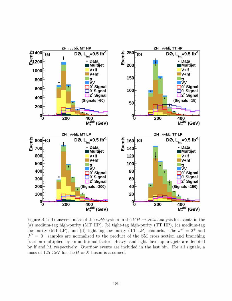
(GeV)bZbTM

0 200 400

Eve

nts

0

200

400

600

800

1000

1200

1400 -1=9.5 fbint

DØ, L

60)×(Signals

DataMultijetV+lfV+hftt

VV Signal+0 Signal-0 Signal+2

, MT HPbbνν→ZH

(a)

(GeV)bZbTM

0 200 400E

vent

s

0

50

100

150

200

250 -1=9.5 fbint

DØ, L

15)×(Signals

DataMultijetV+lfV+hftt

VV Signal+0 Signal-0 Signal+2

, TT HPbbνν→ZH

(b)

(GeV)bZbTM

0 200 400

Eve

nts

0

100

200

300

400

500

600

700

800-1=9.5 fb

intDØ, L

300)×(Signals

DataMultijetV+lfV+hftt

VV Signal+0 Signal-0 Signal+2

, MT LPbbνν→ZH

(c)

(GeV)bZbTM

0 200 400

Eve

nts

0

20

40

60

80

100

120

140

160-1=9.5 fb

intDØ, L

150)×(Signals

DataMultijetV+lfV+hftt

VV Signal+0 Signal-0 Signal+2

, TT LPbbνν→ZH

(d)

Figure B.4: Transverse mass of the ννbb system in the V H → ννbb analysis for events in the(a) medium-tag high-purity (MT HP), (b) tight-tag high-purity (TT HP), (c) medium-taglow-purity (MT LP), and (d) tight-tag low-purity (TT LP) channels. The JP = 2+ andJP = 0− samples are normalized to the product of the SM cross section and branchingfraction multiplied by an additional factor. Heavy- and light-flavor quark jets are denotedby lf and hf, respectively. Overflow events are included in the last bin. For all signals, amass of 125 GeV for theH orX boson is assumed.

189

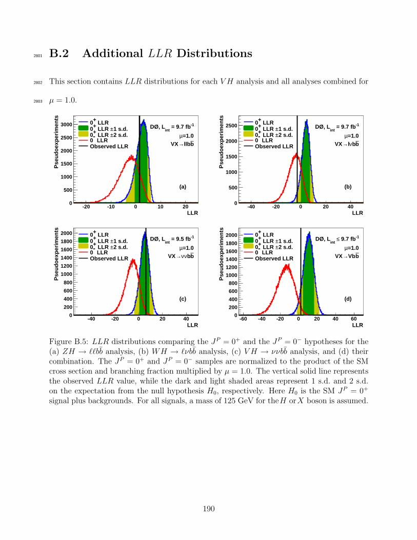
B.2 Additional LLR Distributions2801

This section contains LLR distributions for each V H analysis and all analyses combined for2802

µ = 1.0.2803

LLR-20 -10 0 10 20

Pse

udoe

xper

imen

ts

0

500

1000

1500

2000

2500

3000 LLR+01 s.d.± LLR +02 s.d.± LLR +0

LLR-

0Observed LLR

-1 = 9.7 fbint

DØ, L

=1.0µbllb→VX

(a)

LLR-40 -20 0 20 40

Pse

udoe

xper

imen

ts

0

500

1000

1500

2000

2500 LLR+01 s.d.± LLR +02 s.d.± LLR +0

LLR-

0Observed LLR

-1 = 9.7 fbint

DØ, L

=1.0µbbνl→VX

(b)

LLR-40 -20 0 20 40

Pse

udoe

xper

imen

ts

0

200

400

600

800

1000

1200

1400

1600

1800

2000 LLR+01 s.d.± LLR +02 s.d.± LLR +0

LLR-

0Observed LLR

-1 = 9.5 fbint

DØ, L

=1.0µbbνν→VX

(c)

LLR-60 -40 -20 0 20 40 60

Pse

udoe

xper

imen

ts

0

200

400

600

800

1000

1200

1400

1600

1800

2000 LLR+01 s.d.± LLR +02 s.d.± LLR +0

LLR-

0Observed LLR

-1 9.7 fb≤ int

DØ, L

=1.0µbVb→VX

(d)

Figure B.5: LLR distributions comparing the JP = 0+ and the JP = 0− hypotheses for the(a) ZH → ℓℓbb analysis, (b) WH → ℓνbb analysis, (c) V H → ννbb analysis, and (d) theircombination. The JP = 0+ and JP = 0− samples are normalized to the product of the SMcross section and branching fraction multiplied by µ = 1.0. The vertical solid line representsthe observed LLR value, while the dark and light shaded areas represent 1 s.d. and 2 s.d.on the expectation from the null hypothesis H0, respectively. Here H0 is the SM JP = 0+

signal plus backgrounds. For all signals, a mass of 125 GeV for theH orX boson is assumed.

190

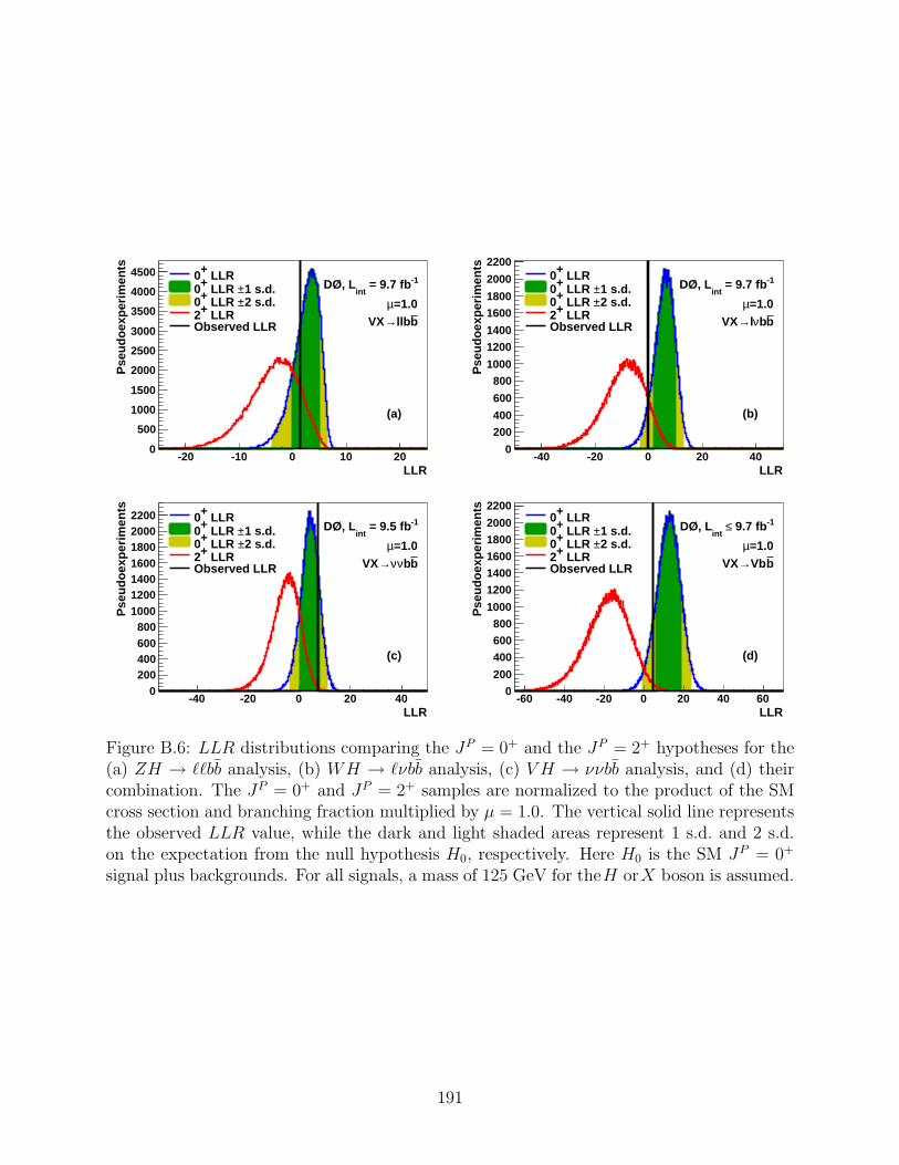
LLR-20 -10 0 10 20

Pse

udoe

xper

imen

ts

0

500

1000

1500

2000

2500

3000

3500

4000

4500 LLR+01 s.d.± LLR +02 s.d.± LLR +0

LLR+2Observed LLR

-1 = 9.7 fbint

DØ, L

=1.0µbllb→VX

(a)

LLR-40 -20 0 20 40

Pse

udoe

xper

imen

ts

0

200

400

600

800

1000

1200

1400

1600

1800

2000

2200 LLR+0

1 s.d.± LLR +02 s.d.± LLR +0

LLR+2Observed LLR

-1 = 9.7 fbint

DØ, L

=1.0µbbνl→VX

(b)

LLR-40 -20 0 20 40

Pse

udoe

xper

imen

ts

0200400600800

1000120014001600180020002200 LLR+0

1 s.d.± LLR +02 s.d.± LLR +0

LLR+2Observed LLR

-1 = 9.5 fbint

DØ, L

=1.0µbbνν→VX

(c)

LLR-60 -40 -20 0 20 40 60

Pse

udoe

xper

imen

ts

0

200

400

600

800

1000

1200

1400

1600

1800

2000

2200 LLR+0

1 s.d.± LLR +02 s.d.± LLR +0

LLR+2Observed LLR

-1 9.7 fb≤ int

DØ, L

=1.0µbVb→VX

(d)

Figure B.6: LLR distributions comparing the JP = 0+ and the JP = 2+ hypotheses for the(a) ZH → ℓℓbb analysis, (b) WH → ℓνbb analysis, (c) V H → ννbb analysis, and (d) theircombination. The JP = 0+ and JP = 2+ samples are normalized to the product of the SMcross section and branching fraction multiplied by µ = 1.0. The vertical solid line representsthe observed LLR value, while the dark and light shaded areas represent 1 s.d. and 2 s.d.on the expectation from the null hypothesis H0, respectively. Here H0 is the SM JP = 0+

signal plus backgrounds. For all signals, a mass of 125 GeV for theH orX boson is assumed.

191

B.3 Expected and Observed p-values for µ = 1.232804

Analysis ZH → ℓℓbb WH → ℓνbb ZH → ννbb Combined

JP = 0− vs. JP = 0+

p0−

test Expected 0.046 0.012 0.005 <0.0001

p0−

test Observed 0.072 0.245 0.0006 0.0051 − pnull Expected 0.500 0.500 0.500 0.5001 − pnull Observed 0.615 0.971 0.215 0.922

CLs Expected 0.908 (1.33 s.d.) 0.975 (1.96 s.d.) 0.989 (2.31 s.d.) 0.9998 (3.60 s.d.)CLs Observed 0.883 (1.19 s.d.) 0.747 (0.67 s.d.) 0.997 (2.78 s.d.) 0.995 (2.56 s.d.)

JP = 2+ vs. JP = 0+

p2+

test Expected 0.037 0.003 0.009 <0.0001

p2+

test Observed 0.078 0.056 0.003 0.0021 − pnull Expected 0.500 0.500 0.500 0.5001 − pnull Observed 0.679 0.937 0.363 0.911

CLs Expected 0.925 (1.44 s.d.) 0.995 (2.56 s.d.) 0.983 (2.11 s.d.) 0.9999 (3.86 s.d.)CLs Observed 0.885 (1.20 s.d.) 0.941 (1.56 s.d.) 0.991 (2.35 s.d.) 0.998 (2.91 s.d.)

Table B.1: Expected and observed p-values and CLs values for JP = 0− and JP = 2+ VX

associated production, assuming signal cross sections equal to the 125 GeV SM Higgs pro-duction cross section multiplied by µ = 1.23. The null hypothesis is taken to be the sum ofthe SM Higgs boson signal and background production.

192

REFERENCES

193

REFERENCES

[1] E. W. Weisstein, Cylindrical coordinates, From MathWorld – A Wolfram Web Resource.

[2] E. W. Weisstein, Spherical coordinates, From MathWorld – A Wolfram Web Resource.

[3] O. Chamberlain, E. Segre, C. Wiegand, and T. Ypsilantis, Phys. Rev. 100, 947 (1955).

[4] K. A. Olive et al., [Particle Data Group], Chinese Physics C 38, 090001 (2014).

[5] H. D. Politzer, Phys. Rev. Lett. 30.

[6] D. J. Gross and F. Wilczek, Phys. Rev. Lett. 30, 1343 (1973).

[7] S. L. Glashow, Nucl. Phys. 22, 579 (1961).

[8] S. Weinberg, Phys. Rev. Lett. 19, 1264 (1967).

[9] A. Salam, Originally printed in *Svartholm: Elementary Particle Theory, ProceedingsOf The Nobel Symposium Held 1968 At Lerum, Sweden*, Stockholm 1968, 367-377.

[10] P. W. Higgs, Phys. Rev. Lett. 13, 508 (1964).

[11] F. Englert and R. Brout, Phys. Rev. Lett. 13, 321 (1964).

[12] G. S. Guralnik, C. R. Hagen, and T. W. B. Kibble, Phys. Rev. Lett. 13, 585 (1964).

[13]

[14] M. Baak et al., The European Physical Journal C 74 (2014).

[15] G. Abbiendi et al., [ALEPH, DELPHI, L3, and OPAL Collaborations, the LEP WorkingGroup for Higgs Boson Searches], Phys. Lett. B 565, 61 (2003).

[16] S. Heinemeyer, C. Mariotti, G. Passarino, and R. Tanaka (Eds.), [LHC Higgs CrossSection Working Group], CERN-2013-004 (2013).

194

[17] T. Aaltonen et al., [CDF and D0 Collaborations], Phys. Rev. D 88, 052014 (2013).

[18] T. Aaltonen et al., [CDF and D0 Collaborations], Phys. Rev. Lett. 109, 071804 (2012).

[19] G. Aad et al., [ATLAS Collaboration], Phys. Lett. B 716, 1 (2012).

[20] S. Chatrchyan et al., [CMS Collaboration], Phys. Lett. B 716, 30 (2012).

[21] Nucl. Phys. B 193.

[22] H. Murayama, UCB-PTH-00/05 (2000), Pedagogical review SUSY review given at 1999ICTP Summer School.

[23] G. Branco et al., Phys. Rep. 516, 1 (2012).

[24] A. Djouadi, Phys. Rep. 459, 1 (2008).

[25] L. Randall and R. Sundrum, Phys. Rev. Lett. 83, 3370 (1999).

[26] L. Randall and R. Sundrum, Phys. Rev. Lett. 83, 4690 (1999).

[27] F. Abe et al., [CDF Collaboration], Phys. Rev. Lett. 74, 2626 (1995).

[28] S. Abachi et al., [D0 Collaboration], Phys. Rev. Lett. 74, 2422 (1995).

[29] S. Abachi et al., Nucl. Instrum. Methods Phys. Res. A 338, 185 (1994).

[30] V. Abazov et al., Nucl. Instrum. Methods Phys. Res. A 565, 463 (2006).

[31] R. Angstadt et al., Nucl. Instrum. Methods Phys. Res. A 622, 298 (2010).

[32] S. Chatrchyan et al., [CMS Collaboration], Phys. Rev. D 89, 092007 (2014).

[33] G. Aad et al., [ATLAS Collaboration], Phys. Lett. B 726, 120 (2013).

[34] A. Martin, W. Stirling, R. Thorne, and G. Watt, The European Physical Journal C 63,189 (2009).

[35] W. J. Stirling, private communication.

195

[36] D. Miller, S. Choi, B. Eberle, M. Mhlleitner, and P. Zerwas, Phys. Lett. B 505, 149(2001).

[37] J. D. Richman, CALT-68-1148 (1984).

[38] J. Ellis, D. S. Hwang, V. Sanz, and T. You, J. High Energy Phys. 2012, 134 (2012).

[39] V. M. Abazov et al., [D0 Collaboration], Phys. Rev. Lett. 109, 121803 (2012).

[40] T. Aaltonen et al., [CDF Collaboration], Phys. Rev. Lett. 109, 111804 (2012).

[41] J. Pumplin et al., J. High Energy Phys. 07, 012 (2002).

[42] T. Sjostrand, S. Mrenna, and P. Skands, J. High Energy Phys. 2006, 026 (2006).

[43] R. Brun and F. Carminati, Cern program library long writeup w5013.

[44] J. Alwall et al., J. High Energy Phys. 2014 (2014).

[45] P. Aquino, K. Hagiwara, Q. Li, and F. Maltoni, J. High Energy Phys. 2011, 1 (2011).

[46] K. Hagiwara, J. Kanzaki, Q. Li, and K. Mawatari, Eur. Phys. J. C 56, 435 (2008).

[47] A. Djouadi, J. Kalinowski, and M. Spira, Computer Phys. Comm. 108, 56 (1998).

[48] M. L. Mangano, F. Piccinini, A. D. Polosa, M. Moretti, and R. Pittau, J. High EnergyPhys. 2003, 001 (2003).

[49] V. Abazov et al., Phys. Lett. B 669, 278 (2008).

[50] E. E. Boos, V. E. Bunichev, L. V. Dudko, V. I. Savrin, and V. V. Sherstnev, Phys.Atom. Nucl. 69, 1317.

[51] A. Hoecker et al., PoS ACAT, 040 (2007).

[52] T. Junk, Nucl. Instrum. Methods Phys. Res. A 434, 435 (1999).

[53] A. L. Read, J. Phys. G 28, 2693 (2002).

196

[54] W. Fisher, FERMILAB-TM-2386-E (2006).

[55] W. C. Fisher, private communication.

[56] T. Andeen et al., FERMILAB-TM-2365 (2007).

[57] N. Kidonakis, Phys. Rev. D 74, 114012 (2006).

[58] U. Langenfeld, S. Moch, and P. Uwer, Phys. Rev. D 80, 054009 (2009).

[59] J. M. Campbell and R. K. Ellis, Phys. Rev. D 60, 113006 (1999).

[60] J. M. Campbell, R. K. Ellis, and C. Williams, Mcfm - monte carlo for femtobarnprocesses.

[61] J. M. Campbell, FERMILAB-Conf-01/072-T .

[62] V. M. Abazov et al., [D0 Collaboration], Phys. Rev. D 88, 052011 (2013).

[63] V. M. Abazov et al., [D0 Collaboration], Phys. Rev. Lett. 109, 121804 (2012).

[64] V. M. Abazov et al., [D0 Collaboration], Phys. Lett. B 716, 285 (2012).

[65] V. M. Abazov et al., [D0 Collaboration], Phys. Rev. Lett. 113, 161802 (2014).

[66] T. Aaltonen et al., [CDF Collaboration], Phys. Rev. Lett. 114, 141802 (2015).

[67] T. Aaltonen et al., [CDF Collaboration], Phys. Rev. Lett. 109, 111803 (2012).

[68] T. Aaltonen et al., [CDF Collaboration], Phys. Rev. Lett. 109, 111805 (2012).

[69] T. Aaltonen et al., [CDF and D0 Collaborations], Phys. Rev. Lett. 114, 151802 (2015).

197