CONSTRAINT SATISFACTION AS A SUPPORT FOR

DECISION MAKING IN SOFTWARE AGENTS

A Dissertation

Presented for the

Doctor of Philosophy

Degree

The University of Memphis

Arpad Gyula Kelemen

August, 2002

ii

DEDICATION

To Yulan Liang

iii

Acknowledgement

I am most grateful to my advisor, Dr. Stan Franklin, who made my work possible

on the IDA project and guided me through my research and development. I also thank

Dr. Mohammed Amini, Dr. Dipankar Dasgupta, Dr. E. Olusegun George, Dr. Art

Greasser, Ravikumar Kondadadi, Dr. Robert Kozma, Yulan Liang, Dr. King­Ip (David)

Lin, Irina Makkaveeva, Dr. Lee McCauley and the “Conscious” Software Research

group, who developed IDA for their invaluable help.

iv

Abstract

Kelemen, Arpad Gyula. Ph.D. The University of Memphis. August, 2002. Constraint Satisfaction as a Support for Decision Making in Software Agents. Major Professor: Stan Franklin, Ph.D.

The U.S. Navy has been trying for many years to automate its personnel

assignment process. Periodic assignment of personnel to new jobs is mandatory

according to Navy policy of sea/shore rotation. Though various software systems are

used regularly, the process is still mainly done manually and sequentially by Navy

personnel, called detailers. An Intelligent Agent, IDA has been designed and

implemented, which applies cognitive theories and new AI techniques to produce flexible

adaptive human­like software. Inside IDA, the constraint satisfaction module is

responsible for satisfying the requirements of Navy policies, command needs and sailor

preferences. In order to enhance decision quality various methods are created,

investigated, tuned and implemented, which are of primary concern to this dissertation.

These methods combine benefits of operational research, cognitive science, neural

networks, fuzzy systems, and statistics. Results show that high level human like

decisions are possible in a noisy, rapidly changing environment under time pressure

within an intelligent agent framework.

Key words: job assignment, distribution, constraint satisfaction, decision making,

matching, intelligent agent, soft constraints, feedforward neural network, adaptive neuro­

fuzzy inference system, support vector machine, adaptive Bayes classifier, consciousness.

v

Table of Contents

List of Tables ........................................................................................................... viii

List of Figures............................................................................................................ ix

1 Introduction .............................................................................................................1

2 IDA........................................................................................................................10

2.1 IDA Architecture .............................................................................................10

2.2 IDA Cycle........................................................................................................16

2.2.1 Deliberation...............................................................................................20

2.2.2 Final Selection According to Ideomotor Theory .........................................21

2.2.3 Creating a Message, Offering a Job (Language Generation Module).........22

2.2.4 Negotiation ................................................................................................23

3 Constraint Satisfaction in IDA................................................................................24

3.1 Three Phases of Constraint Satisfaction in IDA................................................25

3.2 The Constraint Satisfaction Module in IDA......................................................26

3.3 Implementation ................................................................................................31

3.4 Missing Data....................................................................................................36

3.5 “Conscious” Constraint Satisfaction in IDA .....................................................38

3.6 Increasing the Efficiency of the Constraint Satisfaction....................................42

3.6.1 Survey Preference Rankings.......................................................................42

3.6.2 Survey Preferences with Values .................................................................44

3.6.3 Grouping the Stakeholders’ Preferences ....................................................44

3.7 Keeping the Constraint Satisfaction Up­to­Date ...............................................47

4 Neural Networks ....................................................................................................49

4.1 Data Acquisition and Preprocessing .................................................................49

4.2 Design of Neural Network ................................................................................53

4.2.1 Feedforward Neural Network with Logistic Regression..............................53

4.2.2 Neural Network Selection and Criteria ......................................................54

4.2.3 Learning Algorithms for FFNN ..................................................................58

4.2.4 Support Vector Machine ............................................................................59

4.3 Data Analysis and Results................................................................................61

vi

4.3.1 Estimation of Coefficients for Soft Constraints ...........................................62

4.3.2 Neural Network for Decision Making.........................................................63

4.3.3 Comparison of Estimation Tools ................................................................66

4.4 Conclusion.......................................................................................................70

5 Adaptive Neuro­Fuzzy Inference System ...............................................................73

5.1 Design of Adaptive Neuro­Fuzzy Inference System .........................................75

5.2 Results and Rule Extraction .............................................................................77

5.3 Forming Hypothesis on Detailer Decisions.......................................................88

5.4 Offering Multiple Jobs to Sailors......................................................................92

5.5 Conclusion.......................................................................................................93

6 Adaptive Generalized Estimation Equation with Bayes Classifier...........................95

6.1 Classification Model ........................................................................................96

6.1.1 GEE Model for Correlated Data ................................................................96

6.1.2 Modeling Noise and Outliers with Gibbs Sampling Under Bayesian

Framework..............................................................................................................98

6.1.3 Adaptive Bayes Classifiers and Algorithm for Correlated Data Combining

GEE with Additive Noise Model ............................................................................100

6.1.4 Algorithm Summary .................................................................................101

6.1.5 AGEE with Gibbs Sampling under Bayesian Framework with AB Classifier

..............................................................................................................................103

6.2 Experiment Results and Discussion................................................................104

6.3 Comparison of Methods .................................................................................108

6.4 Matching Multiple Sailors to Multiple Jobs....................................................111

6.5 General Performance of AB with AGEE ........................................................112

6.5.1 Adaptive Generalized Estimation Equation for a Second Survey on the

Aviation Support Equipment Technician Community .............................................112

6.5.2 Adaptive Generalized Estimation Equation for the Aviation Machinist

Community ............................................................................................................117

6.5.3 Adaptive Generalized Estimation Equation for Microarray Data .............119

6.6 Conclusion.....................................................................................................120

vii

7 Conclusion...........................................................................................................122

7.1 What Has Been Done .....................................................................................122

7.2 What Has Been Learned.................................................................................123

7.3 How to Integrate the Discussed Modules into IDA.........................................126

References ...............................................................................................................129

Author's Related Publications...................................................................................137

viii

List of Tables

3.1 Sailor’s data 37

3.2 Job’s data, function values, and fitness values 38

4.1 Hard constraints 52

4.2 Soft constraints 52

4.3 Estimated coefficients for the soft constraints with FFNN 62

4.4 Factorial array for model selection for MLP with structural learning 64

4.5 Correlation Coefficients of inputs with outputs for MLP 65

5.1 Typical triangle membership function values for the inputs 81

5.2 Extracted "mined" rules through fast Apriori algorithm 83

5.3 Fuzzy rules after rule extraction 84

5.4 Rules to be used by detailers on soft constraints 90

5.5 Rules to be used by detailers on soft constraints in linguistic terms 91

6.1 Parameter estimates using AGEE 105

6.2 Estimated coefficients (AS community) 105

6.3 Exchangeable correlation matrix 105

6.4 Mixture Gaussian Distribution Estimation from denoised data 106

6.5 The noise data estimation using Gibbs sampling 106

6.6 Correct classification rates for different approaches 109

6.7 Average Running Times, average Correct Decision Making Rates 110

6.8 The list of incorrect decisions made by AGEE based on the first survey 113

6.9 The list of incorrect decisions made by AGEE based on the second survey 114

6.10 Estimated coefficients for the second data set (AS community) 117

6.11 Estimated coefficients (AD community) 119

ix

List of Figures

2.1 Global workspace 11

2.2 Action selection in IDA 14

2.3 The IDA Architecture 15

4.1 Correct classification rates for MLP and Logistic regression 66

4.2 Errorbar plots for MLP, Logistic Regression and SVM 68

4.3 Typical MSE of training and cross­validation with the best MLP 69

4.4 Performance of different training algorithms 70

5.1 ANFIS network architecture with its generated rules 79

5.2 A typical learning curve for triangular membership functions 80

5.3 ANFIS network architecture after rule extraction 85

5.4 Testing results after rule extraction 86

5.5 Learned surface plot on input 1 and input 2 86

5.6 Learned surface plot on input 1 and input 3 87

1

1 Introduction

One important problem many organizations, especially the military forces, face is

the job assignment problem. Typically, a service person is posted to an assignment for a

fixed period of time (like 2­5 years) and then move on to some other job. It is crucial that

the right job is assigned to the right person to achieve optimality. For instance, in the

United States Navy, groups of experts, called detailers, are responsible for the job

assignment task for sailors. However, many, often conflicting, criteria complicate the

assignment process: on one hand, jobs needed to be assigned according to the ability of

the personnel; on the other hand, the needs of the assignee, like the reluctance to be

posted to jobs far away from home for too long, have to be addressed also. This makes

job assignment a challenging, yet crucial task. Although various software programs are

routinely used to enhance the process, decisions are made manually. Any technique that

can automate this process can prove invaluable for the Navy’s personal management unit.

The Navy's deep concern for quality assignments is expressed in their slogan (as a

subtitle of the Sailor 21 document, which summarizes their vision of the 21st century

sailor): "Keep the sailor happy and the Navy ready".

The task of job assignment can be viewed as a classification problem. Thus, to

automate the classification process we need to build a model. However, this task is

complicated by many factors. Firstly, the various criteria, or constraints, can be soft, hard

and semi­hard. Secondly, different navy experts (detailers) may provide fairly different

decisions, due to their personal experience, the sailor community (a community is a

collection of sailors with similar jobs and trained skills) they handle and the current

2

environmental situation, not to mention emotions and mistakes. Thirdly, the data is

highly correlated. On one hand detailer decisions are highly correlated and virtually non­

deterministic, for example detailers typically offer no more than one job for sailors. Also

one detailer estimated that a 20% difference would occur in the decisions even if the

same data would be presented to the same detailer at a different time. On the other hand,

many attributes in the databases contain overlapping data. Some can be directly derived

from others. For example, “reverse paygrade” can be derived from “paygrade”. Some

contain refined information of other attributes, such as rating (community) and rate

(community with paygrade). Others are just naturally correlated with each other, like

“paygrade” and “Navy Enlisted Classification codes” (trained skills). All these included

indeterminate subjective components, making the constraint satisfaction and prediction of

the job assignment a very sophisticated and challenging task.

The job assignment problem is not a new problem. Although traditional models

work very well for stationary models where situations don't change and the preferences

are well defined. However in cases where decisions have to be made on noisy, rapidly

changing environment based on limited knowledge under time pressure traditional

models don't work well. The use of agent (Franklin & Graesser, 1997) architectures

opens a new direction in artificial intelligence, where decisions can be made and actions

can be selected, in rapidly changing, noisy, uncertain environments, and the goal is

shifted from optimality to satisfaction. One approach to designing such agents is to build

them after minds, particularly after human minds, which are the main source of

intelligence today. Building intelligent agents and software not only aims at problem

3

solving by itself, but also gives us a new tool to deepen our understanding of minds, and

intelligence, which is perhaps the ultimate power in the universe.

As a novel approach to the Navy's job assignment problem, an Intelligent

Distribution Agent (IDA) (Franklin, Kelemen, & McCauley, 1998) has been built by the

"Conscious" Software Research Group at the University of Memphis. IDA not only deals

with the job assignment problem as a pure decision making problem, but as a complete

automation process starting from receiving email messages from sailors and ending with

the production of orders, and is designed to handle any emerging unseen situations. For

this purpose IDA is equipped with about a dozen large modules, each of which is

responsible for one main task. One of them, the constraint satisfaction module, is

responsible for satisfying constraints to ensure the adherence to Navy policies, command

requirements, and sailor preferences. Constraint satisfaction and decision making in IDA

are delicate and ever changing processes, much like human decision making.

A number of approaches have been proposed, implemented and tested in order to

model the Navy's job assignment problem. Among others, an evolutionary approach was

discussed by Kondadadi, Dasgupta, and Franklin (2000). Genetic algorithms can be used

for any optimization problem, but running time could be high to evolve an efficient

model. Yet evolutionary techniques offer the advantage of adaptation to environmental

changes and may deal with data with outliers. A large­scale network model was

developed by Liang and Thompson (1987), Liang and Buclatin (1988), Ali, Kennington,

and Liang (1993). Their work offers a unique operations research technique to deal with

multi objective optimization problems such as the Navy's job assignment problem. Their

model was developed to assign a set of sailors to a set of jobs simultaneously instead of

4

individual sailors to suitable jobs one at a time. Although theoretical results were quite

encouraging, testing on real world Navy data under time pressure did not provide good

results. This partially justifies our choice to attempt constraint satisfaction on a one sailor

to multiple jobs bases. Also, detailers currently do constraint satisfaction in this manner

and IDA is intended to do just like a detailer, including constraint satisfaction. Other

typical constraint satisfaction models such as goal network programs, the stable marriage

model (Gale & Shapley, 1962), the simplex method or linear programming do not work

well for data with high level of noise. Moreover, our model should aim at being adaptive

to the ever­changing environment, as well as the ever­evolving demands towards the

decision maker, which should be learned and adapted to also.

To better model humans IDA's constraint satisfaction is implemented through a

behavior network (Maes, 1990; Maes, 1992; Song & Franklin, 2000; Negatu & Franklin,

to appear). Combination with Baars' theory of "consciousness" is also explored and

implemented, which can help to handle novel situations and resource management

(Baars, 1988, 1997). The model employs a linear functional approach to assign fitness

values to each candidate job for each candidate sailor. The functional yields a value in

[0,1] with higher values representing higher degree of "match" between the sailor and the

job. Some of the constraints are soft, while others are hard. Soft constraints can be

violated without invalidating the job. Associated with the soft constraints are functions,

which measure how well the constraints are satisfied for the sailor and the given job at

the given time, and coefficients which measure how important the given constraint is

relative to the others. The hard constraints cannot be violated and are implemented as

Boolean multipliers for the whole functional. A violation of a hard constraint yields 0

5

value for the functional. The major task to make this approach work requires periodic

tuning of the coefficients and less frequently, the functions.

In order to automate the decision making process in IDA for quality assignments

we need a model, which can make optimal or nearly optimal decisions and is able to

maintain those over time with little or no human supervision. This requires adaptation to

environmental changes (such as economic changes, Navy policy changes,

wartime/peacetime changes, etc.) including unseen situations. With periodic use of data

coming from human detailers, the agent may learn to make better and up to date human­

like decisions, which follow environmental changes with some delay. Moreover IDA

could also learn to make better decisions through online experience with sailors.

However, to test the efficiency of the latter, we need to measure Navy and sailor

satisfaction, rather than the percentage of decisions that agree with the human expert

provided data.

To obtain good results appropriate data acquisition, preprocessing, and suitable

model selection are critical. With certain post­processing model performance can be

further improved. In this work, various types of neural networks, neuro­fuzzy systems

and modern statistical models that learn detailer­like decisions are designed, implemented

and compared.

One approach is to use neural networks and statistical methods to enhance

decisions made by IDA's constraint satisfaction module and to make better decisions in

general. The functions for the soft constraints were set up in consultation with Navy

experts. While human detailers can make judgements about job preferences for sailors,

they are not always able to quantify such judgements through functions and coefficients.

6

Using data collected periodically from human detailers, a neural network learns to make

human­like decisions for job assignments. Different detailers may attach different

importance to constraints, depending on various factors and may change from time to

time as the environment changes. It is important to set up the functions and the

coefficients in IDA to reflect these characteristics of the human decision making process.

A neural network provides better insight on what preferences are important to a detailer

and how much. The inevitable changes in the environment will result changes in the

detailer's decisions, which could be learned with a neural network although with some

delay. Feedforward Neural Networks with logistic regression, Multi Layer Perceptron

(MLP) with structural learning and Support Vector Machine with Radial Basis Function

(RBF) as network structure were explored to model decision making. Statistical criteria,

like Mean Squared Error, Minimum Description Length, etc. were employed to search for

best network structure and optimal performance. Sensitivity analysis through choosing

different algorithms to assess the stability of the given approaches was performed.

Perhaps most resembling to the human decision making process an Adaptive

Neuro­Fuzzy Inference System (ANFIS) is discussed, which can be very suitable for

surveys of Navy experts and uses fuzzy membership functions for soft constraints to

reflect satisfaction degrees. The goal is to find the most appropriate control actions

(decisions resulting from fuzzy rules) for "matches" between jobs and sailors. Further

goal is to extract a small number of fuzzy rules, which are still very effective without

giving up robustness.

ANFIS as a possible new IDA module may adapt to environmental changes (such

as economic change, Navy policy change, wartime/peacetime change, etc.), unseen

7

situations, and increase efficiency. Moreover with periodic use of data coming from

human detailers, the system may learn to make better and up to date human­like

decisions, which can also follow environmental changes with some delay.

Even though human detailers may face some difficulties in defining real valued

functions and numeric coefficients to be applied in IDA’s current linear functional model,

the use of fuzzy membership functions and values is convenient, because detailers can

easily express their decisions in terms of linguistic descriptions (such as high, medium,

low) in regard to constraints as well as to the overall fitness of the match between sailors

and jobs.

Currently there are about 320,000 enlisted personnel in the U.S. Navy. Each year

more then 100,000 Navy enlisted personnel are assigned to new jobs at a cost of some

$600 million dollars just for moving expenses. Other costs apply, too. In general, the

process whereby personnel managers direct the movement of individuals to fill vacancies

in field activities is called distribution.

The distribution of sailors is done by some 280 Navy personnel (detailers). Each

detailer makes assignments for a community of typically between 1,000 and 5,000

sailors. A community consists of sailors of the same rating, for example: Aviation

Support Equipment Technicians (AS). Besides constraint satisfaction, a detailer’s task is

quite complex. Communicating with sailors and other agents (human and non­human)

via natural language, reading and maintaining databases, using various software

programs, searching for jobs for sailors, producing orders are some of the tasks a detailer

might do in order to perform his/her task. Our goal is to automate most ­ if not all ­ of the

tasks performed by a human detailer using an intelligent agent architecture, which

8

requires little or no human supervision and is able to run through time. Our agent has

modules for perception (natural language understanding), working and associative

memories, emotions, learning, “consciousness”, action selection, constraint satisfaction,

deliberation, and negotiation by means conversing with sailors and others via email in

natural language. We have designed and implemented a “conscious” software agent,

called, Intelligent Distribution Agent (Franklin, Kelemen, & McCauley, 1998) who is

intended to do the job of a human detailer efficiently while modeling human cognition.

Also keep in mind that one main goal in Artificial Intelligence is to produce intelligent

software that can think and act intelligently, comparable to humans. One approach is to

follow psychological theories of cognition in implementing intelligent systems. "If you

want to understand something then build it."

This dissertation describes the design and implementation of IDA. The main

focus is on constraint satisfaction as a support for decision making in a real time real

world environment.

The proposed research aims to achieve several specific goals. Some of its

contributions to engineering and science are the following:

• Design and implementation of a working constraint satisfaction model within the

intelligent agent framework, which is able to support decision making efficiently.

• Design, implementation, and testing of a wide variety of machine learning

approaches in order to enhance constraint satisfaction efficiency.

• Design and implementation of an innovative ensembling approach for

classification and prediction, which combines advanced statistical learning

models and data mining techniques.

9

• Design and implementation of a "conscious" version of constraint satisfaction

model, which fits cognitive modeling of humans within a cognitive agent

architecture.

• Build a hypothesis on how detailers make decisions and how humans do

constraint satisfaction.

• Build a hypothesis on what makes a biological or artificial agent intelligent.

• Contribution to the research in intelligent agents and machine learning with

publications.

The rest of the paper is organized as follows. Chapter 2 provides an overall

description of the IDA architecture, briefly discussing the key modules and presenting a

typical cycle of the agent. Chapter 3 describes the process of constraint satisfaction and

the emerging theoretical and practical issues. Chapter 4 discusses Feed Forward Neural

Network and Support Vector Machine approaches to help with constraint satisfaction and

decision prediction, including performance function, statistical criteria and learning

algorithm selection. Chapter 5 surveys a neuro­fuzzy approach and fuzzy rule extraction

for constraint satisfaction and decision prediction. Chapter 6 presents a suitable, but non­

standard statistical approach and provides comparison study of all the discussed methods.

Finally chapter 7 gives some concluding remarks and future directions.

10

2 IDA

2.1 IDA Architecture

An autonomous agent is a system situated within, and part of, an environment.

The system senses that environment, and acts on it, over time, in pursuit of its own

agenda. It acts so as to possibly effect what it senses in the future (Franklin & Graesser,

1997). IDA is not only an autonomous agent but also a “conscious” software agent.

“Conscious” software agents (Ramamurthy, Bogner, & Franklin, 1998; Bogner,

1999; Bogner, Ramamurthy, & Franklin, 2000; Kondadadi, Dasgupta, & Franklin, 2000;

Franklin, 2001) are cognitive agents (Franklin & Graesser, 1997; Franklin, Kelemen, &

McCauley, 1998) that implement Baars’ global workspace theory, a psychological theory

of consciousness (Baars, 1988, 1997).

According to global workspace theory the mind’s architecture includes many

small, specialized processes, which are normally unconscious, and a global workspace (or

blackboard). Baars used the analogy of a collection of experts, seated in an auditorium,

each of whom can solve some problem or problems. It is not known who can solve a

given problem. In global workspace theory somebody makes the problem available to

everyone in the auditorium by putting it on the blackboard. An expert on this particular

problem can identify and solve the problem. One of the main functions of consciousness

is to recruit resources to deal with novel or problematic situations. When a novel

situation occurs, an unconscious process tries to broadcast it to all other processes in the

system by trying to put it on the blackboard, which causes it to become conscious. Only

11

one problem can be on the blackboard at a time. Therefore consciousness is a serial

system.

Figure 2.1 shows the global workspace, the codelets competing to get into

“consciousness” and the unconscious processors who receive the broadcasts.

Figure 2.1 Global workspace

We implement these unconscious processes as codelets borrowing the term from

Mitchell and Hofstadter (1991) and Mitchell (1993). A codelet is a small piece of code

capable of performing some basic task (analogous to an expert in the auditorium).

12

Information codelets are codelets, who carry primitive pieces of information. An

attention codelet is a codelet that “pays attention” to a particular type of event. When

that event happens it collects the right information codelets, and they try to make it to

“consciousness” together in order to broadcast the situation to other codelets.

At any given time, different processes (attention codelets) could be competing

with one another, each trying to bring its information to “consciousness”. These codelets

compete in a place called the playing field. Codelets may form coalitions depending on

the strength of associations between them. The activation (different from association) of

a codelet measures the likelihood of it becoming “conscious”. The coalition with the

highest average activation finds its way to “consciousness.” In the event of a tie the

winner is randomly chosen.

An important task IDA is tooled to do is the ability to negotiate with sailors. IDA

both sends and receives messages in natural languages. It uses the Copycat architecture

(Hofstadter & Mitchell, 1994) for natural language understanding. Copycat has been

designed for analogy making. The knowledge, that IDA needs to understand different

concepts in a message such as the sailor's name, social security number (SSN), idea type,

etc., are stored in the form of a slipnet, a knowledge representation structure similar to a

semantic net. When IDA receives a message from a sailor, the perception codelets

analyze the message and look for patterns, which could be similar to a name, a SSN,

other sailor particulars, and an idea­type. Percepts then are stored in perception registers.

They activate some nodes in the slipnet and finally, depending on the perceived idea type,

a template is chosen and filled with the information obtained in the message. IDA also

has to do active perception, which means that she has to go out and search for

13

information and knowledge herself. For example she can retrieve and perceive

information from Navy personnel, job and training databases.

Another central module in IDA is the behavior network (Maes, 1990; Song &

Franklin, 2000; Negatu & Franklin, to appear) for high­level action selection in the

service of built­in drives. IDA has several distinct drives operating in parallel. These

drives vary in urgency as time passes and the environment changes. Behaviors are

typically mid­level actions, many depending on several primitive actions for their

execution. A behavior net is composed of behaviors and their various links. A behavior

looks very much like a production rule, having preconditions as well as additions and

deletions. Each behavior occupies a node in a digraph. The three types of links,

successor, predecessor and conflictor, of the digraph are completely determined by the

behaviors. Activation is passed via these links and behaviors are chosen for execution

according to a previously agreed strategy having to do with highest activation. A

behavior network is also similar to Minsky’s agents’ society (Minsky, 1987).

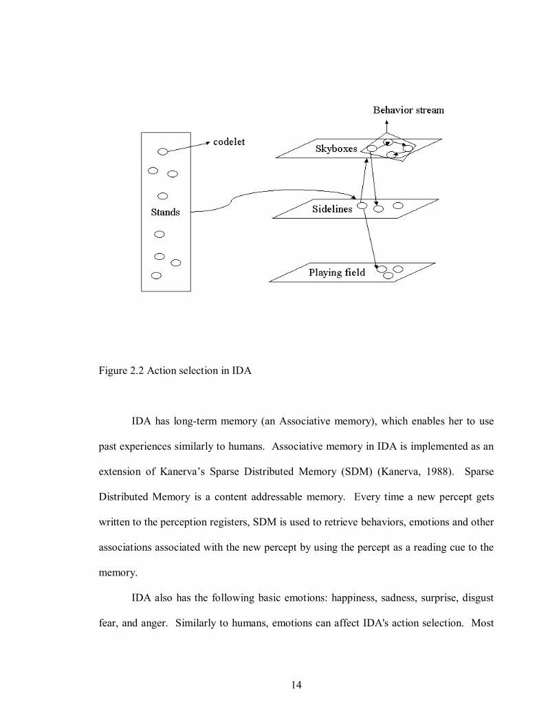
The action selection mechanism in IDA is shown in figure 2.2. When a

“conscious” broadcast is made, all the codelets in the stands receive it. A codelet jumps

to the sidelines if the broadcast contains information relevant for that codelet. This type

of codelet is called a “behavior priming” codelet. It instantiates a proper goal structure in

the “Skyboxes”, if it is not already there yet. They also try to bind as many variables in

the behaviors as possible, and send activations to behaviors in a goal structure. Each

behavior in the goal structure gets executed via some behavior codelets, who jump into

the playing field.

14

Figure 2.2 Action selection in IDA

IDA has long­term memory (an Associative memory), which enables her to use

past experiences similarly to humans. Associative memory in IDA is implemented as an

extension of Kanerva’s Sparse Distributed Memory (SDM) (Kanerva, 1988). Sparse

Distributed Memory is a content addressable memory. Every time a new percept gets

written to the perception registers, SDM is used to retrieve behaviors, emotions and other

associations associated with the new percept by using the percept as a reading cue to the

memory.

IDA also has the following basic emotions: happiness, sadness, surprise, disgust

fear, and anger. Similarly to humans, emotions can affect IDA's action selection. Most

15

of the codelets are part of IDA's emotion network, where different emotion states are

represented by activation spreads among different nodes (McCauley, 1999; McCauley,

Franklin, & Bogner, 1999).

Other modules of IDA will be discussed later.

Figure 2.3 shows the high level architecture of IDA. Note that almost all the

modules feed into the behavior network and the “consciousness” module. The behavior

net feeds into most modules. The modules in the second line typically get executed

sequentially. The constraint satisfaction module is referred to as linear functional.

Figure 2.3. The IDA Architecture

16

2.2 IDA Cycle

To best demonstrate the actual work of IDA let’s go though briefly a typical cycle

(episode) beginning with an email message from a sailor requesting the start of an

assignment process and ending with the composition of a reply message offering the

sailor a choice of one, two, or occasionally three jobs.

CYCLE BEGIN

Suppose the following email message comes from a sailor:

“Date: Tue, 13 Jun 2000 16:53:23 +0000

From: LEGAULT JOHN DOE <doe@navy.mil>

Subject: SSN: 123456789

IDA,

I am AK1 LEGAULT JOHN DOE. Please find me a job.

Thanks,

AK1 LEGAULT JOHN DOE”

The following pieces of data will be perceived from the given email message:

­ message date

­ sailor’s name

­ sailor’s SSN (Social Security Number)

17

­ the sailor is looking for a new job

­ sailor’s contact information

Perception module codelets extract surface features from the message and activate

nodes in the slipnet (Mitchel, 1993). Templates are chosen and the ideas are perceived.

The understood data (information) from the message is written to the workspace (short­

term memory) from and to which various modules can write and read. It's also written to

the perception registers, a part of the focus. The focus is part of the workspace, which is

used to write to and read from the long­term memory, implemented as a Sparse

Distributed Memory (SDM) (Kanerva, 1988). Every time the workspace is updated the

focus is updated. A read (retrieval of associations) from SDM happens every time the

focus is updated, using part of the focus chosen based on activation levels. We use a

mechanism that uses probabilities and thresholds. Activation levels are set to 1 for each

new item written to the focus. Activations for all the fields in the focus are decaying

according to a decay mechanism. The range of the activation levels is [0, 1].

Associations coming back from SDM are written to the second layer of the focus.

Information/attention codelets sitting in the stands (auditorium) see the message

in the workspace and instantiate copies of themselves that get the information from the

message. At the same time an attention codelet sitting in the stands looking at the

workspace recognizes the idea of the new message, gathers the correct

information/attention codelets, increases his activation, and they all jump to the playing

field.

18

The coalition manager (Bogner, 1999) forms a coalition of codelets based on

associations. Some initial associations are built in, while others are learned. Hopefully

the codelets from the previous paragraph will form a coalition. The spotlight controller

(Bogner, 1999) selects the coalition with the maximum average activation, and shines the

spotlight on it. In other words the codelets in the spotlight are the ones whose contents

are in “consciousness”. The broadcast manager (Bogner, 1999) broadcasts all the

information carried by the codelets in the spotlight. After their information is broadcast,

all the codelets in the spotlight leave the playing field.

Some behavior priming codelets sitting in the stands find the broadcast relevant,

bind their variables using the information in the broadcast and jump to the sidelines, a

special part of the playing field. Using the auditorium analogy, the behavior priming

codelets are the experts who identify the problem and know how to solve it, but they

don’t solve it themselves, instead they initiate the problem solving process.

Some coalition of codelets instantiates an appropriate goal structure (unless it's

already instantiated), binds as many variables as it can, and sends activation

(environmental link) to the initial behavior of the goal structure. A goal structure is a

chunk of IDA’s behavior network (Maes, 1990), which consists of linked behaviors,

environmental states, goals and drives (Franklin, 1995). Each goal structure is trying to

satisfy a drive or a goal. In the example cycle, the first goal structure will look up the

sailor's personnel record.

The behavior net eventually chooses and executes the initial behavior of the goal

structure, causing it to instantiate codelets to create an SQL (Standard Query Language)

query to access the sailor's personnel record for the relevant fields, one field at a time.

19

Behaviors get performed by codelets, called behavior codelets. The task of one behavior

is typically done by one to four behavior codelets.

After the first behavior is selected an emotion and an action are written to the

focus. With the current content of the focus, taking decay into consideration, IDA writes

to SDM. The result of this query, the content of a single field, is copied to the

corresponding fields in the workspace and the focus (internal perception). This triggers

another SDM read of associations with this data. Attention codelets provoke another

broadcast containing these contents. The answering behavior priming codelets send

activation eventually causing another behavior in the goal structure to execute another

query, yielding the content of another field that is again written to the workspace and

focus. (Another write has occurred during this time.) This process continues until all the

required fields are written into the workspace.

Then a different goal structure recovers information from the requisition list

(current items from the job database). Upon execution this goal structure instantiates

codelets to create SQL queries to access the relevant fields with matching Navy Enlisted

Classification (NEC) (job qualifications) and matching paygrade resulting in a coarse

selection of say ten to fifteen possible jobs. The same process through "consciousness"

and the behavior network is used to retrieve each field. Again, the results of these queries

are copied to the corresponding fields in the workspace (internal perception), with the

requisite reads from and writes to long­term memory.

Yet another goal structure sends in turn each job from the coarse selection to the

linear functional (constraint satisfaction module) to receive its fitness value. The process

20

is again the same. As a result, the fitness values will be written to the workspace beside

the corresponding jobs.

2.2.1 Deliberation

An attention codelet watching the workspace notices that all the jobs listed there

have fitness values assigned to them. It picks the job with the highest fitness value,

gathers information codelets for the job, jumps into the playing field, forms a coalition

and, hopefully, gets its message broadcast. Behavior priming codelets in the stands find

the broadcast relevant, jump to the sidelines, and instantiate a goal structure “To create a

scenario for the job”. Using our behavior net process as above, a possible detach date

from the sailor’s current job is calculated and written to the workspace by a behavior

codelet using the Projected Rotation Date. Another attention codelet notices this detach

date and starts the process that adds leave time to the scenario. Similarly, travel time and

proceed time (if needed) are added. The gap between the date the job should be filled in

and the date the sailor would report to the job is calculated, and the scenario building

process is started anew if needed.

This process of scenario building continues until an appropriate number of jobs

are selected for offer to the sailor, or until there are no more jobs with sufficiently high

fitness about which to build a scenario. However voluntary action may take over when

the first scenario is finished and offer only one job.

21

2.2.2 Final Selection According to Ideomotor Theory

The players in this part of the drama are attention/emotion codelets who have

preferences for jobs with certain attributes. One might be concerned with keeping

moving costs down, another with job priority, and still another with the size of the arrival

gap. Some might be concerned with two of these attributes. Another player is the

timekeeper codelet to be described below.

At any time after at least one scenario has been completed, one of these

attention/emotion codelets can propose a particular job that has a completed scenario. To

do so he gathers information about which job he is proposing and brings it to

"consciousness," if he can. In the stands is the timekeeper codelet. If enough time passes

without an objection to this job or without the proposal of another job, the timekeeper

marks the proposed job as one to be offered. This process can continue until two, or even

three, jobs have been marked.

On the other hand, one of these attention/emotion codelets might choose to object

or to propose a different job to be offered. This is done in the same way, with the

attention/emotion codelet gathering information and coming to "consciousness." In the

case of a new proposal, it simply replaces the old proposal, but with a reduction in the

timekeeper's patience, and is handled in the same way. An objection, unless soon

followed by a new proposal, or a re­proposal of the original (with less activation to get to

"consciousness"), results in another scenario initiated by the attention codelet who has

been competing with proposers for “consciousness.”

22

After a proposal is accepted, the process continues until three are accepted, or

until no more scenarios are being created and the timekeeper is out of patience. He then

calls a halt, setting a flag to this effect in the workspace.

2.2.3 Creating a Message, Offering a Job (Language Generation Module)

The appropriate attention codelet notices the end of job selection flag and begins

the message generation process by gaining "consciousness" with the appropriate

information codelets (sailor's name, paygrade, etc).

The same action selection process recruits a codelet who writes the first paragraph

of the message, the appropriate salutation, into the workspace. Another attention codelet

gains "consciousness" with the salutation and with the number of jobs to be offered. The

same action selection process results in the second paragraph, the introduction, being

written into the workspace. This whole process repeats until paragraphs for each job to

be offered and a closing paragraph are written into the workspace (the message). IDA

signs her name, and sends the message using the same action selection process.

CYCLE END

This completes our description of a typical IDA cycle. However, IDA keeps

running and other emails may come in, which initiate new cycles.

23

2.2.4 Negotiation

Besides offering jobs to sailors, IDA's language generation module has to send

out emails about various subjects, most of the time as a response to incoming emails.

Using the same mechanism described above IDA is able to respond to emails and

situations of a large variety. Many of these messages would be about requests from

sailors and can be answered in scripts, such as requests for additional data, or request for

waiting until the next requisition list (job list) arrives. Different kinds of scripts are

needed for different kinds of message types, but even for the same message type IDA is

able to respond in different ways. For example an angry emotion, or a close sailor PRD

may trigger an email more forceful in order to push the sailor towards a decision. This is

similar to what human detailers may do, and models human behavior and cognition well.

With the constraint satisfaction module’s place in the process laid out, we turn to

a detailed description.

24

3 Constraint Satisfaction in IDA

As we have seen before the U.S. Navy currently employs some 320,000 enlisted

sailors. Periodic reassignment of such sailors is mandatory according to Navy policy.

When new assignments are considered, a considerable number of constraints should be

satisfied. The constraints can be divided into groups in various ways. One such way is

whose interest they serve. Some constraints are to comply with general Navy policies,

others serve command preferences, and still others care about sailor happiness. These

stakeholders’ interests often contradict, which results in a multi­objective optimization

problem.

Constraints can also be divided into hard, soft, and semi­hard ones. Hard

constraints must be satisfied and they are designed to conform to strict Navy policies.

Violation of a hard constraint makes a sailor not eligible for the given job within the

decision­making time frame. While soft constraints are desired to be satisfied, violation

is acceptable, and partial satisfaction is often granted. Soft constraints are designed to

increase sailor happiness and to satisfy those Navy policies that are not hard. Semi­hard

constraints have to be satisfied, but sailor eligibility can be earned before the new

assignment takes place. The bulk of the constraint satisfaction falls into the soft

constraints. Setting up soft constraints and their relative importance is a very delicate and

ever­changing process. We need a common currency function, which can compare

monetary, timing, happiness and efficiency issues against one another. Unfortunately

Navy policies may easily change from one week to the next and economy, manning, war­

time, and other situation changes may require frequent tuning of our constraint

25

satisfaction model. A natural evolution in Navy planning, design, and technology may

lay ahead in order to further objectives.

3.1 Three Phases of Constraint Satisfaction in IDA

Constraint satisfaction in IDA currently happens in three separate phases. The

first is called coarse selection, which happens when IDA is looking for jobs for a given

sailor using certain criteria. If a job doesn’t match all the criteria specified in the SQL

query then it doesn’t get chosen. IDA uses community match, so only those sailors are

selected who are in the right community. Much of the data is taken from the Navy’s

Assignment Policy Management System’s (APMS) sailor, job, and training databases,

which are actively integrated with IDA. The APMS databases provide information about

more than 10,000 sailors and 30,000 jobs at a given time. IDA proceeds with the coarse

selection and writes the passing jobs to the workspace. Once the coarse selection is over

the second phase of the constraint satisfaction takes place.

The second phase of the constraint satisfaction is done with a linear functional

and from now on we call this phase the “constraint satisfaction”. As we will see below a

functional assigns normalized fitness values (fitness) for each job in the workspace for

the given sailor at the given time considering several additional constraints. Once the

linear functional is finished, each job in the workspace will have a fitness value assigned

to it.

Then the third phase of the constraint satisfaction takes place, what we call

deliberation. In the deliberation module as we have seen above temporal scenarios are

26

created for the high fitness jobs. On the basis of these scenarios jobs are proposed and

some of them may be accepted for offering to the sailor. Issues like timing, training,

costs and feasibility are taken care of in the deliberation module. Emotions also play an

important role in this module. Once created scenarios get proposed, rejected, and

accepted (James, 1890; Franklin 2000; Kondadadi, 2001; Kondadadi & Franklin, 2001).

3.2 The Constraint Satisfaction Module in IDA

Though the Navy has about 600 constraints (issues), about 500 of them apply only

to small groups of jobs and sailors. They cover extreme circumstances and are seldom

considered by a detailer. The remaining, approximately, 100 constraints bear very

different importance, and different detailers may consider different ones more important

then others, even if handling the same community. Changing the community may largely

change the importance of constraints, and as time goes by there is a natural change in

their relevance too.

As we have seen above constraints can be differentiated into hard, soft and semi­

hard ones. The constraints can also be divided into three classes according to whose

interest they serve: sailor, command, and Navy constraints.

Some of the sailor constraints are:

­ Location preference (sailor wants to be stationed in a certain place)

­ Billet preference (sailor wants to serve on a specific ship/command)

­ General training preference (sailor wants training)

­ Negative general training preference (sailor doesn’t want training)

27

­ Specific training preference (sailor wants training for a specific skill)

­ Negative specific training preference (sailor doesn't want training for a specific

skill)

­ Preference for sea service (sailor wants to be at sea)

­ Preference for shore service (sailor wants to be on shore)

­ Promotion (sailor wants promotion opportunity)

­ Schooling for child (sailor wants schooling for his/her child)

­ Exceptional Family Member (sailor has family member who needs special care)

The first three are the most typical, most reasonable requests from sailors and the

most respected ones by detailers and IDA.

Some of the command constraints are:

­ Paygrade preference (command may want the sailor to have different paygrade

than the one on the requisition list)

­ NEC match (Sailor has appropriate job skills)

­ PCS cost (sometimes the command pays for moving cost under certain

circumstances)

­ Gap (depending on the billet the command may prefer overlap or exact match)

­ Remaining obligated service (when will the sailor's obligated service expire)

­ Job priority (some jobs are more important to be filled than others at a given

time. This is Navy policy, but the command may prefer some jobs to be filled in before

and after job priorities are set).

28

­ Command preference for a particular sailor (command may prefer sailors based

on information not available in the databases)

­ Preference for multiple sailor skills (command wants sailor with multiple skills

(NECs), who can perform more than one task)

­ Sailor is in a certain age group

­ Woman in ship (some billets are only available for men)

Some of the Navy constraints are:

­ Paygrade match (sailor’s paygrade has to match the job’s paygrade)

­ PCS cost (Permanent Change of Station cost, keep down moving costs)

­ Geographic location (it is better to assign a sailor in the same geographic

location where he/she currently serves)

­ NEC reutilization (it is better to assign a sailor to a job with his existing NECs

(trained skills) without needing further training

­ Fleet Balance (the Navy sets a quota for the number of enlisted people for the

Pacific, Atlantic coast and other branches, and it’s bad to go above or below it. If the

manning difference between two branches is larger than 5% then it’s better to assign a

sailor to the branch with lower manning).

To consider all the constraints simultaneously we need a common currency

function, which compares time with money, sailor preferences with Navy policies and so

on. To account for all the constraints simultaneously a linear functional is applied (a

29

convenient abuse of language with the hard constraints as products) with the following

form:

) 1 . 2 . 3 ( ) ( * )) ( ( ) ( ~ 1 ~ 1 ~ j m j

n

j j i

m

i i x f a x c x F +

= = ∑ ∏ = ,

where

~ i x (i = 1,…,m+n) are input vectors of variables, which are not necessarily

disjoint in their variables and ~ x is the union of all the variables occurring in all the

~ i x s.

i c (i = 1,…,m) is a Boolean function for the i'th hard constraint; it yields 1 if

the corresponding hard constraint is satisfied, otherwise it yields 0.

j f (j = 1,…,n) is a function for the j’th soft constraint; it yields values in

[0,1] (the closed unit interval of real numbers).

j a (j = 1,…,n) is a coefficient, constant in [0,1] for the j’th soft constraint.

The equation

) 2 . 2 . 3 ( 1 1

= ∑ =

n

j j a

guarantees that F will yield values in [0,1]. This will also be useful later for tuning

purposes (the actual setup of the coefficients).

30

Every j f is a function which measures how well the j’th soft constraint is

satisfied if we were to offer the given job to the given sailor at the given time. These

functions are monotonic, but not necessary linear, however often they are. Setting up

these functions is based on community specific knowledge, up to date Navy policies, and

common sense. Detailers, who handle communities are the most useful source of

information. Tuning of these functions can also be done through learning.

Every aj tells how important is the j'th soft constraint in relation to the others.

This gives the common currency property, where we can specify which constraint we

care about most at a given time frame.

Note that if a hard constraint is satisfied then it doesn’t change the value of F, but

if it is not then F is equal to 0, which means that the sailor doesn’t match the given job, so

he is not eligible for it. F = 1 would mean the ideal job for the sailor, which practically

never happens due to the long functional and the self­contradicting constraints.

After the sailor’s particulars are in the workspace behavior codelets of the

constraint satisfaction module calculate all the function values for each of the constraints

for one job and write them to the workspace, where other modules can access it as well.

Once all the values are in place a different behavior codelet calculates and writes the final

fitness to the workspace. The process continues until all the jobs have fitness values

assigned. Once each job is assigned a fitness value, the deliberation module may build

temporal scenarios on high fitness jobs over threshold in order to find jobs for final

offering to the sailor. Note that different sailors in the same community are subject to the

same F functional at a given time frame.

31

3.3 Implementation

IDA was implemented in JAVA using JDK 1.3 and tested on machines with a

333MHz Pentium­II processor and 64 MB RAM and above with Windows 2000

environment. However, some modules have huge resource demands to run properly,

therefore we test IDA on a 1.8GHz Pentium­IV with 2 GB RAM. To access real sailor,

job and other data, IDA was integrated with various Navy databases, lookup tables, and

software to do certain tasks.

Currently there are 11 behavior codelets for 11 soft constraints and 4 behavior

codelets for 4 hard constraints. Constraints are listed on the left side, and the

corresponding behavior codelets with the functions they implement are in parenthesis on

the right side. An approximate description of the function definitions are also provided.

The exact definitions are too extensive and technical to be provided.

Soft Constraint: Behavior codelet and function id:

1. Job Priority Match (CalculateJobPriorityMatch.java, f1)

Each job in the job database has a priority. The higher the job priority the more

important it is to fill in the job. Accordingly the function assigns f1 = 1 if the job priority

is 1, and linearly decreasing to 0 for job priority 51. Jobs with priority 52 or above also

get f1 = 0 assigned.

2. Order Cost Match (CalculateOrderCostMatch.java, f2)

This is the moving cost. The lower the cost the better the match. If the moving

cost is $0 then f2 = 1, and it linearly decreases to f2 = 0 for $30,000, and stays 0 over this

32

amount. Moving costs are provided by the Navy’s autocost software, which IDA uses. It

calculates moving costs from distance between locations, paygrades, and the sailor's

number of dependents.

3. Location Preference Match (CalculateLocationPreferenceMatch.java, f3)

A sailor may express his preference for a given location in an email message or in

the Job Advertisement and Selection System (JASS), which eventually gets written in

databases. The sailor’s primary, secondary and tertiary preferences are kept for sea,

shore and overseas locations using Area Type Codes (ATC). This function checks to see

if the ATC of the sailor’s preference matches the considered job’s ATC. If the sailor’s

email request is matched or if the database’s primary preference is matched then f3 = 1, if

the secondary preference is matched then f3 = 0.95, if the tertiary then f3 = 0.90, and in

case of no match f3 = 0. However, f3 = 0.85 default value gets assigned in case the sailor

provided no location preference. Note that IDA is equipped to transfer location

preferences expressed in natural language in a large variety of forms into ATCs. This

includes abbreviations, capitalization, Navy slang, and large area parsing into ATCs such

as east coast, Europe, Norfolk, etc.

4. NEC Reutilization Match (CalculateNECReutilizationMatch.java, f4)

Up to five Navy Enlisted Classification (NEC, skills acquired via training) codes

are kept in Navy personnel databases of enlisted people. Jobs may ask for up to two

NECs. No sailor can get a job without an NEC required by the job, though having both is

not required. This function assigns f4 = 1 if the sailor already has a required NEC and 0

otherwise with some exceptions. Note that even though this looks like a hard constraint,

this really is a soft constraint because NECs may be earned via training, which will be

33

considered later in the deliberation module. As a soft constraint it is a valid one because

the Navy generally tries to reutilize existing NECs in order to avoid unnecessary training.

5. Paygrade Match (soft) (CalculatePaygradeMatch.java, f5)

This function assigns f5 = 1 if the sailor’s paygrade equals the job’s preferred

paygrade, and various values for other cases. If the sailor’s paygrade is off by more than

one from the job’s paygrade then typically f5 = 0.

6. Georgraphic Location Match (CalculateGeographicLocationMatch.java, f6)

This function assigns f6 = 1 if the sailor’s current ATC is the same as the

proposed job’s ATC and various other values for other cases.

7. Training Match (CalculateTrainingMatch.java, f7)

This function assigns high values if the sailor's training preference can be

satisfied, and low values if not.

8. Job Denial Match (CalculateJobDenial.java, f8)

This function assigns f8 = 1 if the sailor has already denied the given job before,

and f8 = 0 otherwise.

9. Sailor Preference Match (CalculateSailorPreferenceMatch.java, f9)

This constraint is to handle sailor location preferences expressed in emails in any

form. The corresponding function assigns high values if the constraint is satisfied and

low values if not. Tuning this function is very complex and it will be eventually

integrated with f3.

10. Sea Shore Preference Match (CalculateSeaShorePreferenceMatch.java, f10)

This function assigns high values if the sailor's sea/shore preference can be

satisfied and low values otherwise.

34

11. Duty Preference Match (CalculateDutyPreferenceMatch.java, f11)

This function assigns high values if the sailor's billet preference can be satisfied

and low values otherwise.

The distance from the Projected Rotation Date (PRD) is also integrated into the

soft constraints. Negotiation for jobs normally takes place between 9 and 6 months

before the new assignment. As the date gets closer to the 6­month window, the functions

concerned with sailor satisfaction yield lower values, eventually dropping to 0. When the

6­month window is reached a job gets selected for the sailor, which the sailor must

accept.

Hard Constraint: Behavior codelet and function id:

1. Sea Shore Match (CalculateSeaShoreMatch.java, c1)

According to Navy policy if a sailor served on shore then his next assignment

must be on sea and vice versa. This function returns 1 if the considered job satisfies the

“sea/shore rotation” policy. Otherwise it returns 0.

2. Dependents Match (CalculateDependentsMatch.java, c2)

This function returns 1 if the considered sailor and job satisfies the “No more than

three dependents to overseas location” policy. Otherwise it returns 0.

3. Paygrade Match (PaygradeMatch.java, c3)

This function returns 1 if the considered sailor and job paygrades are not too far

from each other (typically at most one paygrade away).

35

4. Teaching for E4 Match (CalculateTeachingForE4Match.java, c4)

This function returns 0 if the considered job would require a sailor with E4

paygrade to teach. Otherwise it returns 1.

The definitions of the functions were based on information provided by detailers.

Each of the above functions yield normalized real values on [0,1]. Each of them are

tuned such a way that 0 and 1 values are obtainable. Each of them read the necessary

fields from the workspace, convert them to the right numeric format, do modifications on

them and then assign them conditionally as a value to functions.

The presented constraints are some of those most frequently considered ones by

detailers. Other constraints are applied in the coarse selection and in the deliberation

modules. To settle which hard constraints to consider in the coarse selection and which

in the linear functional we follow cognitive modeling of detailers and cost efficiency.

Note that some constraints overlap each other, while others just correlate. For example

the Order Cost Match and the Geographic Location Match are highly correlated, yet

according to current Navy practices they both get evaluated independently to help

decision making.

It turned out that in many cases discrete "linear" functions handle constraints well.

The vast majority of jobs get discarded because of a failing hard constraint in both the

coarse selection and the linear functional. On the other hand, soft constraints by

themselves practically never make a fitness value 0. To get a fitness value of 1 is

practically impossible. The deliberation module considers jobs with fitness over

threshold, which is currently set to 0.45. Finally note that the three phases of constraint

36

satisfaction could be done in one, but for both cognitive modeling and task efficiency we

choose not to do so. The three significantly different phases also give us a better

overview and control over the agent.

Right now there are no separate codelets for semi­hard constraints. The issue of

semi­hard constraints is worked out with the help of the deliberation module. As of now

we treat semi­hard constraints as soft constraints and set a flag to warn the deliberation

module about it. The “CalculateFitness.java” behavior codelet calculates the final fitness

value for each candidate job using values calculated by other functions. It applies

normalized on [0,1] real coefficients, where the sum of the coefficients (ai’s) is 1. This

results in normalized fitness (f) values, which are measures to express the fitness between

jobs for sailors. Setting up the coefficients correctly is a major problem, which is

investigated in the forthcoming chapters.

3.4 Missing Data

What to do if a data item about a constraint is empty? The most frequent missing

data is in the sailor’s preferences. If the corresponding constraint is a hard constraint then

IDA should ask the corresponding stakeholder (Navy, Command, Sailor) to provide its

preference if applicable. If some other piece of information is not available then IDA

should write an email to the right office or assume that the constraint is satisfied. Such

decisions are up to the detailer. A detailer can learn how to deal with situations like

these, so should IDA. If the constraint is a soft constraint then IDA should assume that

the stakeholder has no preference, and the corresponding constraint is highly satisfied. A

37

value close to 1 (currently 0.85) indicates that the constraint is satisfied, but not as well as

if it was explicitly asked for and satisfied. A further possible method is discussed in the

next section. The version presented below handles preferences in a more flexible way.

Not specifying certain preferences may emphasize the relevance of other preferences of

the same stakeholder as a side effect.

Table 3.1 shows some of the sailor’s data, which is used by the constraint

satisfaction. The data contains the followings: SeaShore code, NEC1­5, Number of

dependents, Location preference from email, Sea Location Preference 1­3, Shore

Location Preference 1­3, Overseas Location Preference 1­3, Area Type Code, Paygrade

respectively.

Table 3.1. Sailor’s data

1 7606 7609 1 GMY GPS FNO GPS GKE GMY BER CUB GUM ELA 6

Table 3.2 shows seven simplified examples for job data and fitness values which

are used by the constraint satisfaction. The data contains the followings: SeaShore code,

Area Type Code, Paygrade, NEC1­2, Job Priority, Order Cost, value for c1, c2, f1­f5,

functions, and finally F, the overall fitness value. Note that a1 = a2 = a3 = a4 = a5 = 0.2

coefficients were used for demonstration.

38

Table 3.2. Job’s data, function values, and fitness values

2 FNO 6 7612 1 450 1 1 1 0.985 0.9 0 1 0.777 2 FNO 5 7617 2 450 1 1 0.98 0.985 0.9 0 0.1 0.593 2 FNO 5 7618 5 450 1 1 0.92 0.985 0.9 0 0.1 0.581 2 ING 6 7618 4 2520 1 1 0.94 0.916 0 0 1 0.571 2 FNO 6 7609 8 450 1 1 0.86 0.985 0.9 1 1 0.949 2 FNO 6 7606 7 450 1 1 0.88 0.985 0.9 1 1 0.953 3 ICE 6 7609 10 3490 1 1 0.82 0.884 0 1 1 0.741

3.5 “Conscious” Constraint Satisfaction in IDA

IDA currently has two versions of the constraint satisfaction module: an

unconscious and a “conscious” one. In the case of the unconscious constraint satisfaction

only one attention codelet goes to “consciousness”, the one, which realizes that the

perception module has finished its job. In the “conscious” version each needed sailor and

job data item goes to “consciousness” as well as the value for each hard constraint, soft

constraint and the final fitness for each job.

The constraint satisfaction module can be viewed as an external module from a

cognitive agent, because it’s a little bit hard (but not impossible) to find it’s true parallel

in a human agent who calculates functions, and applies various coefficients to come up

with a normalized real value to measure the “goodness” of a possible job for a given

sailor at a given time. On the other hand, every detailer must have his own judgment to

consider various constraints in order to decide which jobs are suitable for a sailor. A

detailer may do such decisions unconsciously, but usually it is a conscious decision. This

is comparable to a linear functional approach of the constraint satisfaction problem in

IDA.

39

Because of the more than 300 parallel running java threads taking up resources,

the long delay cycles in some of them to conform to the “consciousness” module, the

large sized emotion network, the usage of a graphical interface for demonstration

purposes, and various other reasons, running IDA on a 1.8GHz Pentium­IV machine is

somewhat time consuming. It takes about 8 minutes for a typical, long ("Find me a job"

idea type) cycle, which is comparable to human performance. The use of "conscious"

constraint satisfaction increases this time to about 15 minutes.

Once the data is written into the workspace the constraint satisfaction module

assigns the same values weather it is “conscious” or not, and it runs through only once.

Therefore the usage of “conscious” constraint satisfaction doesn’t buy us anything other

than cognitive modeling. On the other hand, when IDA is prepared to handle all kinds of

emails and situations, “conscious” constraint satisfaction may be useful. Consider the

following situation: after an incoming message from a given sailor asking for a job, IDA

has performed a cycle, found two suitable jobs and offered them to the sailor. Now a

new email comes from the same sailor saying that he doesn’t like either of the jobs and

asks why he wasn’t offered a particular third one. Now IDA needs to find out why she

didn’t offer the job to the sailor earlier. The answer can’t simply be “the fitness of the

job was too low for you”; she needs to find out exactly why. If IDA did constraint

satisfaction unconsciously then she needs to go through it with the same data consciously,

in order to find out where the sailor missed the most points and why. Note that she can

only do this if she has access to the same data. Such data might be recovered from SDM,

because it was written there during the first run (because everything what goes to

"consciousness" goes to SDM too). Once the reason is found, the negotiation module can

40

produce the proper answer with the main reason or reasons. Notice that this highly

resembles what a human detailer would do; therefore for cognitive modeling it is the right

thing to do. However the issue of efficiency requires more discussion. The cost of

“consciousness” is high, so avoiding it for the first pass in the constraint satisfaction

seems justified. For the second pass the same unconscious module would never produce

a detailed answer, only the fitness, which is not enough to answer the sailor’s second

question.

As opposed to the previous two­pass system, in a one pass system where the

constraint satisfaction always happens consciously, the needed data might be written to

long term memory, and could be recovered later from there, but not with absolute

certainty (just like from a human memory). To do so, a “very conscious” constraint

satisfaction is necessary, which is not only “conscious” of the data, and the fitness, but

also of each of the ci hard constraints and the fi soft constraints for each job as well as the

ai coefficients. A further question about the two­pass constraint satisfaction is how to

reconstruct the same data for the second pass. By the time IDA is about to do the

“conscious” constraint satisfaction some of the data might be gone. The sailor’s data is

probably still available with no change in the database, but the job data might have lost

some significant piece of information, for example the job priority or even the job itself is

not in the database any more. To recover such data might be possible from the agent’s

own long term memory. Whether IDA tries to recover data from a database or from long

term memory the probability of recovering the data grows less with time. If IDA

receives the sailor’s new email after a new requisition list has arrived then the old data is

lost and she no longer has access to the same data about the job in the database. On the

41

other hand, if IDA receives the sailor's second email before a new requisition list arrives,

chances are that she will have access to all the data as before and therefore be able to find

an answer to the sailor’s question. All this means that IDA should send job offers to

sailors as soon as possible to give them plenty of time to ask about it. If the answer

comes early, IDA also has a better chance of being able to recover the context from

memory.

Another issue is that as time goes by the situation is no longer the same.

Considering a job for a sailor now is often very different from considering it two weeks

later. For example the constraint satisfaction might consider the Projected Rotation Date

(PRD) as one issue, meaning that the closer the PRD the more important it is to find a job

for the sailor. So, if you consider it a month later then higher fitness values should occur

in order to find a job for the sailor quickly, which effectively decrease the value of other

considerations. However, most of the time related issues (constraints) are handled in the

deliberation module. In the current implementation the constraint satisfaction module

can’t recover decisions made by the deliberation module. Recovering such decisions

should be done by the deliberation module or some other module; making the constraint

satisfaction module do so makes no sense.

A third possible way to answer the sailor’s second email would require some

external storage. Though on some important issues a detailer does make some notes for

himself, it is inefficient and inappropriate to keep track of every single piece of datum,

and every single decision he makes in files in terms of speed and memory. For cognitive

modeling it is clearly not a possibility.

42

3.6 Increasing the Efficiency of the Constraint Satisfaction

Methods presented in this subsection have not been implemented yet, though

might be useful for future implementations in order to increase efficiency, and

stakeholder satisfaction.

3.6.1 Survey Preference Rankings

Based on feedback from all the three stakeholders the linear functional can yield

more accurate and up to date results. If we hold a survey where each stakeholder ranks

its preferences, the coefficients can be set accordingly. The sum of a stakeholder’s

coefficients is prefixed and is subject to detailer or Navy supervision, and the sum of all

coefficients is 1.

For example, suppose the sailor ranks his constraints as follows:

1. Sailor wants training

2. Sailor wants to be in a certain place

3. Sailor wants to be on a specific ship

etc.

This means that the sailor’s most important constraint (preference) is to get

training, the second one is to be in a certain place, etc.

43

Similarly the command constraints:

1. Job priority

2. Paygrade preference

3. Preference for multiple sailor skills

etc.

and the Navy constraints:

1. NEC reutilization

2. Paygrade match

3. PCS cost

etc.

Once IDA has all the rankings, she would transform them into values according to

a previously agreed strategy. For example one strategy might be to set the values linearly

decreasing from 1 to 0, where an imaginary last+first preference gets the value of 0, so

even the last preference (constraint) will get some positive value. Then project the

transformed values to the prefixed quota of coefficients specified by a detailer, the Navy,

or eventually, by IDA.

44

3.6.2 Survey Preferences with Values

As an addition to the rankings, IDA may even ask each stakeholder to assign a

value to the constraints on a normalized scale, say on [0,1]. In this case IDA doesn’t

have to transform the rankings into values, only to project them to the prefixed quota of

coefficients. This enables the linear functional to yield more accurate results, because of

the use of more accurate data. For example, if a sailor feels that his first preference is

twice as important as his second one then he should give 1.0 for the first and 0.5 for the

second. Giving equal values to multiple constraints is also possible. Note that the actual

numerical value of a stakeholder’s specifications doesn’t matter because of the

projection; only their relative value matters, and it’s important to let them understand

this. Giving the highest (1.0) value to all of his preferences will not help him in getting a

“better job”, it only means that all of his constraints are equally important for him, giving

0.1 value to all of them means the same thing for IDA.

3.6.3 Grouping the Stakeholders’ Preferences

It is also possible to group the soft constraints for each stakeholder. This would

allow us to conveniently tune coefficients for each stakeholder’s sake and setup general

coefficients for the stakeholders to measure whose happiness is more important at a given

time.

Once all the constraints are given in the transformed (weighted) form for each

stakeholder, we need to set up the general weights for the projection for each of the three

45

stakeholders according to detailer or Navy supervision (eventually IDA). This will tell

which class of constraints is more important in relation to the other two. For example if

the command constraints and the Navy constraints are equally important, and both of

them are twice as important as the sailor’s preferences, then coefficients for the

command, Navy, and sailor’s, preferences respectively are the following: 0.4, 0.4, 0.2.

The projections should be done into them. These relative weights may change from time

to time, or from community to community, and always needs to be set by the Navy, or by

a detailer, and eventually by IDA.

All the rankings and the above values can only be applied for the soft constraints,

which can be violated. Hard and semi­hard constraints, which must be satisfied are not

part of the preferences.

Incorporating the hard constraints and the soft constraints we come up with the

following grouped version of the linear functional, which considers a given job for a

given sailor at a given time:

) 1 . 3 . 6 . 3 ( ) ( * )) ( ( ) ( ~

3

1 ~ 1 ~ j m j j

j i

m

i i x f a x c x F +

= = ∑ ∏ =

and

) 2 . 3 . 6 . 3 ( 1 3

1

= ∑ = j

j a

46

All terms have the same meaning as before with the following changes: j f is a

function which considers all the soft constraints listed by the j'th stakeholder along with

their given values if available, j = 1, 2, 3. We use the transformed values if only rankings

were allowed.

Each aj is a coefficient, which measures the relative importance of the i'th

stakeholder.

The fj functions have the following form:

) 3 . 3 . 6 . 3 ( ) ( ) ( ~ 3

1 ~ k m k

p

k k j m j x g b x f + +

= + ∑ = ,

Every k g is a function (for k = 1, 2, …, p) which measures how well the k’th soft

constraint is satisfied if we were to offer the given job to the given sailor. The range of

all of these functions is [0, 1]. These functions are a priori defined, and are often linear

but not necessarily.

Every k b is a coefficient which tells how important is the k'th soft constraint in

relation to the others for the given stakeholder. All the coefficients are in [0, 1]. These

values (or at least the rankings) are provided by the appropriate stakeholder.

Note that in this version of the constraint satisfaction the only control a

stakeholder has over the module lies in the k b coefficients. The j f function incorporates

all of the j'th stakeholder’s preferences. The k g functions are a priori set, though some

47

additional survey may provide further information in order to better design them. In

many cases they are linear. F is different for each sailor in the corresponding j f part, but

the same F must be used for all jobs for the same sailor.

3.7 Keeping the Constraint Satisfaction Up­to­Date

Once IDA (and the linear functional) is online, qualified Navy personnel (possibly

a detailer) may monitor the functions’ decisions and provide feedback. This can enable

us or IDA to initiate changes when policies change and to tune the functions and the

coefficients in order to make more accurate calculations. The feedback could happen in

three ways.

The first way would require code updating by the monitor. Updating only the

coefficients is relatively easy. Changing existing functions isn’t much harder, but

introducing or deleting constraints may require a lot more effort due to the complex

design of IDA. New behavior, attention, and information codelets may become

necessary, which is not trivial, especially in the “conscious” version of the constraint

satisfaction. Whole new goal structures have to be created, which is not easy. New

tuning of the coefficients also becomes necessary as a side effect.

The second way would only require a high level, but formal specification, say an

XML file, of the required changes in the constraint satisfaction module. XML can be

easily learned by any human detailer. IDA is already prepared to parse XML files for the

action selection module, but now it needs to be tooled to do the same for constraint

48

satisfaction, to create or delete behaviors, and goal structures, and update old ones,

effectively operating on java files.

The third, ideal, way would be to learn online through both natural language

feedback and metacognition. Again, IDA needs to be tooled to create and delete

behaviors, and goal structures, and update old ones for constraint satisfaction. However,

to see the results of such actions, assuming that IDA runs in a real environment, may take

a long time even if she changes only one function at a time. Note that this strategy may

work for other parts of the agent, but not as obviously as in the constraint satisfaction

module, where input­output pairs are fairly deterministic, and can be easily traced. Some

written history of the agent’s actions and some internal modules may help in early tuning.

Unfortunately, even the Navy faces difficulties in measuring the performance of

detailers, so the tuning might differ from one detailer to the other. No final ideal setup is

possible. The change in Navy policies, the economy, manpower availability, peace and

wartime situations, etc. makes the tuning more difficult and unavoidable. IDA needs to

be highly adaptive especially in regard to constraint satisfaction where key decisions are

made for the sake of the stakeholders.

In spite of all the difficulties, keep in mind that the ultimate goal of this project

and of much of artificial intelligence in general is to create an agent that can perform

efficiently with very little or no human supervision in a real world environment.

49

4 Neural Networks

One natural way the decision making problem for quality assignments in IDA can

be addressed is via the tuning the coefficients for the soft constraints. This will spare the

agent's architecture from growing more complex, and it saves on both running time and

memory. In this chapter we show how neural networks can be used to learn coefficients

for the linear functional.

Decision making can also be viewed as a classification problem, for which neural

networks have been demonstrated to be a very suitable tool. Neural networks can learn to

make human­like decisions, and would naturally follow any changes in the data set as the

environment changes, eliminating the task of re­tuning the coefficients. In this chapter

we also show how neural networks can be used to replace the linear functional in IDA

and compare it with the use of neural networks as a support to tune the coefficients.

In this section we survey design, implementation, and testing issues of Feed­

Forward Neural Networks and Support Vector Machines with the aim to approximate

detailer decisions either via learning coefficients for the existing constraint satisfaction

module or via decision classification. Comparison study of the surveyed methods is also

provided to see which can yield better approximation of decisions made by detailers.

4.1 Data Acquisition and Preprocessing

Data was obtained from the US Navy’s Assignment Policy Management System’s

job and sailor databases. For the study one particular community, the Aviation Support

50

Equipment Technicians community was chosen. Note that this is the community on

which the current IDA prototype has been built. The databases contained 467 sailors and

167 possible jobs for them. Each database has more than 100 attributes, such as sailor

name, sailor paygrade, sailor location preferences, job paygrade, job location code and so

on. The data first was pre­processed and cleaned, eliminating unnecessary and

superfluous attributes. This results with 18 attributes from the sailor database and 6 from

the job database. Hard constraints then are employed to filter away the inappropriate

“matches” between sailors and jobs. After that the functions representing soft constraints

are applied. The function values served as inputs to the neural networks and other

models.

For this study four hard and four soft constraints were used, which are widely

considered by detailers. These four soft constraints are the most often considered by

detailers. Many soft constraints are not applicable for all "matches" between sailors and

jobs, but the selected ones are always applicable. Also the selected soft constraints are

the ones, that the Navy provided data for in sufficient quantity for experiment so far.

Generation of fake data for more constraints was also considered but was not

implemented in order to avoid unbalances and other biases in the data, in the datailer

surveys, and in the machine learning methods. Table 4.1 shows the four hard constraints,

which were applied to these attributes in compliance with Navy policies. 1277 matches

passed the given hard constraints, which were inserted into a new database.

Table 4.2 shows the four soft constraints applied to the "matches" that satisfied

the hard constraints and the functions, which implement them. These functions measure

degrees of satisfaction of matches between sailors and jobs, each subject to one soft

51

constraint. Note that some details about the constraints are omitted in both Table 4.1 and

Table 4.2. The detailed constraints are used in the experiment to construct the data set

and to build the models. All the fi functions are monotone but not necessarily linear.

Note that monotonicity can be achieved in cases when values are assigned to set elements

(such as location codes) by ordering. After preprocessing the function values, which

served as inputs to future processing, were defined using information given by Navy

detailers. Each of the function's range is [0,1]. Output data (decisions) were acquired

from an actual detailer in the form of Boolean answers for each possible match (1 for jobs

to be offered, 0 for the rest) and he was asked to make decisions based only on the

constraints given in table 4.1 and table 4.2. Decisions were made sequentially and

independently. This simulates the typical task a detailer normally faces: offer a job or

jobs to a given sailor at the given time from a given list of possible jobs, not considering

other sailors, jobs which will only be available in the future, etc. Of course the sailor

does not have to accept the offered job and various other things might happen before the

job actually gets posted to the sailor. Other modules in IDA are designed to manage

these situations.

Every sailor along with all his/her possible jobs that satisfy the hard constraints

were assigned to a unique group, which is called group ID. This is important because the

outputs (decisions given by detailers) were highly correlated: there was typically one job

offered to each sailor. The numbers of jobs in each group were counted and normalized

to fit the [0,1] unit interval by simply dividing them by the maximum value; this will be

used later for decision refinement. In some experiments they were included in the input

as function f5.

52

Table 4.1 Hard constraints

Function Policy name Policy

c1 Sea Shore Rotation If a sailor's previous job was on shore then he/she is only eligible for jobs at sea and vice versa

c2 Dependents Match A sailor with more than 3 dependents is not eligible for overseas jobs

c3 Navy Enlisted Classification (NEC) Match

The sailor must have an NEC (trained skill) that is required by the job

c4 Paygrade Match (hard)

The sailor’s paygrade cannot be off by more than one from the job's required paygrade

Table 4.2 Soft constraints

Function Policy name Policy

f1 Job Priority Match The higher the job priority, the more important it is to fill the job

f2 Sailor Location Preference Match

It is better to send a sailor to a place he/she wants to go

f3 Paygrade Match (soft) The sailor’s paygrade should exactly match the job’s required paygrade

f4 Geographic Location Match

Based on locations certain moves are more preferable for the Navy than others

53

4.2 Design of Neural Network

4.2.1 Feedforward Neural Network with Logistic Regression

One simple case of FFNN topology is one input layer and one output layer with

logsigmoid function (Schumacher, Rossner, & Vach, 1996), which is equivalent to the

Generalized Linear Model with logistic link function. This can be used to evaluate the

relative importance of functions f1,...,f4 and can be used to tune the coefficients for them.

The conditional probability of the occurrence of the job to be offered is:

) 1 . 1 . 2 . 4 ( ) ( ) | 1 ( ˆ f w g w decision P y T = = =

) 2 . 1 . 2 . 4 ( 1

) ( a

a

e e a g +

=

where g(a) represents the logistic function evaluated at activation a. Let w denote a

weight vector and f the column vector of the importance functions, where f5 is the sailor

group ID:

) 3 . 1 . 2 . 4 ( ] ,..., [ 5 1 f f f T =

Then the “decision” is generated according to the logistic regression model. Note

that the relative importance of the functions will be represented in the values of wi, which

can be used as estimates to the relative importance of the functions in IDA's linear

functional (values of ai). Accuracy of such estimation can be verified through testing.

The weight vector w can be adapted using FFNN topology (Schumacher, Rossner,

& Vach, 1996; Biganzoli, Boracchi, Mariani, & Marubini, 1998). The coefficients for

54

f1,...,f4 can be learned using FFNN with the quasi­Newton method. The estimated

weights satisfy Eq.(4.2.1.4):

) 4 . 1 . 2 . 4 ( 1 0 , 1 ∑ ≤ ≤ = i

i i w w

The linear combination of weights with inputs f1,...,f4 is a monotone function of

conditional probability, as shown in Eq.(4.2.1.1) and Eq.(4.2.1.2), so the conditional

probability of job to be offered can be monitored through the changing of the

combination of weights with inputs f1,...,f4. The classification of decision can be

achieved through the best threshold with the largest estimated conditional probability

from group data. The class prediction of an observation x from group y was determined

by

) 5 . 1 . 2 . 4 ( ) | Pr( max arg ) ( k y x x C k = =

To find the best threshold we used Receiver Operating Characteristic (ROC) to

provide the percentage of detections correctly classified and the non­detections

incorrectly classified. To do so we employed different thresholds with range in [0,1]. To

improve the generalization performance and achieve the best classification, the MLP with

structural learning was employed (Ishikawa, 1996; Kozma, Sakuma, Yokoyama, &

Kitamura, 1996; Miller & Zurada, 1998).

4.2.2 Neural Network Selection and Criteria

Since the data coming from human decisions inevitably include vague and noisy

components, efficient regularization techniques are necessary to improve the

55

generalization performance of the FFNN. This involves network complexity adjustment

and performance function modification. Network architectures with different degrees of

complexity can be obtained through adapting the number of hidden nodes and

partitioning the data into different sizes of training, cross­validation and testing sets and

using different types of activation functions. A performance function commonly used in

regularization, instead of the Sum of Squared Error (SSE) on the training set, is a loss

function (mostly SSE) plus a penalty term (Cun, Denker, & Solla, 1990; Bishop, 1995;

Girosi, Jones, & Poggio, 1995; Haykin, 1999):

) 1 . 2 . 2 . 4 ( 2 ∑ + = w SSE J λ

From another point of view, for achieving the optimal neural network structure

for noisy data, structural learning has better generalization properties and usually use the

following modified performance function (Ishikawa, 1996; Kozma, Sakuma, Yokoyama,

& Kitamura, 1996):

) 2 . 2 . 2 . 4 ( | | ∑ + = w SSE J λ

Yet we propose an alternative cost function, which includes a penalty term as

follows:

) 3 . 2 . 2 . 4 ( / N n SSE J λ + =

where SSE is the sum of squared error, λ is a penalty factor, n is the number of

parameters in the network decided by the number of hidden nodes and N is the size of the

input example set.

56

For achieving the minimized SSE under the constraint or penalty term in

Eq.(4.2.2.3), there is a closed form for the value of N and n. This closed from can be

obtained by taking partial derivatives of the Lagrange multiplier equation if n and N are

continuous. This yields a relationship between N and n and also among N, n and the

SSE. Through structural learning in which the cost function in Eq.(4.2.2.3) is minimized,

we would like to find the effective size of training samples included in the network and

also the best number of hidden nodes for the one hidden layer case. In this study the

value of λ in Eq.(4.2.2.3) is from 0.001 to 1.0. Note that λ = 0 represents a case where

structural learning is not considered, and the cost function reduces into the sum of

squared error. Normally the size of input samples should be chosen as large as possible

in order to keep the residual as small as possible. Due to the cost of the large size

samples, the input may not be chosen as large as desired. However, if the sample size is

fixed then the penalty factor combined with the number of hidden nodes should be

adjusted to minimize Eq.(4.2.2.3).

For achieving the balance between data­fitting and model complexity from the

proposed performance function in Eq.(4.2.2.3) and for better generalization performance

a two­factorial array was designed to dynamically retrieve the best partition of data into

training, cross­validation and testing sets with adapting the number of hidden nodes given

the value of λ. Several statistical criteria were carried out for this model selection in

order to find the best FFNN:

• Mean Squared Error (MSE) defined as the Sum of Squared Error divided

by the degree of freedom. For this model, the degree of freedom is the sample size minus

the number of parameters included in the network.

57

• Correlation Coefficient (r) can show the agreement between the input and

the output or the desired output and the predicted output. In our computation, the latter is

used.

• Akaike Information Criteria (AIC) (Akaike, 1974) defined as

) 4 . 2 . 2 . 4 ( . 2 ) log( 2 ) ( a ml a K L K AIC + − =

• Minimum Description Length (MDL) (Rissanen, 1978) defined as

) 5 . 2 . 2 . 4 ( , log 5 . 0 ) log( ) ( N K L K MDL a ml a + − =

where Lml is the maximum value of the likelihood function and Ka is the number of

adjustable parameters. N is the size of the input examples' set.

The MSE can be used to determine how well the predicted output fits the desired

output. More epochs generally provide higher correlation coefficient and smaller MSE

for training in this study. To avoid overfitting and to improve generalization

performance, training was stopped when the MSE of the cross­validation set started to

increase significantly.

Sensitivity analysis were performed through multiple test runs from random

starting points to decrease the chance of getting trapped in a local minimum and to find

stable results.

The network with the lowest AIC or MDL is considered to be the preferred

network structure. An advantage of using AIC is that a sequence of hypothesis testing

can be avoided when selecting the network. Note that the difference between AIC and

MDL is that MDL includes the size of the input examples which can guide us to choose

appropriate partition of the data into training and testing sets. Another merit of using

58

MDL/AIC versus MSE/Correlation Coefficient is that MDL/AIC use likelihood which

has a probability basis. The choice of the best network structure is based on the

maximization of predictive capability, which is defined as the correct classification rate

and the lowest cost given in Eq.(4.2.2.3).

4.2.3 Learning Algorithms for FFNN

Various learning algorithms have been tested for comparison study, (Bishop,

1995; Tsoukalas & Uhirg, 1997; Haykin, 1999):

• Back propagation with momentum

• Conjugate gradient

• Quickprop

• Delta­delta

The back­propagation with momentum algorithm has the major advantage of

speed and is less susceptible to trapping in a local minimum. Back­propagation adjusts

the weights in the steepest descent direction in which the performance function is

decreasing most rapidly but it does not necessarily produce the fastest convergence. The

search of the conjugate gradient is performed along conjugate directions, which produces

generally faster convergence than steepest descent directions. The Quickprop algorithm

uses information about the second order derivative of the performance surface to

accelerate the search. Delta­delta is an adaptive step­size procedure for searching a

performance surface (Bishop, 1995). Performance results for these methods on our data

59

will be provided later. The performance of the best MLP with one hidden layer network

obtained from above was compared with a popular classification method Support Vector

Machine and FFNN with logistic regression.

4.2.4 Support Vector Machine

Support Vector Machine is a method for finding a hyperplane in a high

dimensional input space that separates training samples into two classes while

maximizing the minimum distance between the hyperplane and any training samples

(Cortes & Vapnik, 1995; Scholkopf, et al., 1997; Cristianini & Shawe­Taylor, 2000;

Muller, Mika, Ratsch, & Tsuda, 2001). A Support Vector Machine can apply any kind of

network structure and typically uses a kernel function with regularization (Friess,

Cristianini, & Campbell, 1998).

SVM has properties to deal with high noise level and flexibly applies different

network architectures and optimization functions. The data used involves relatively high

level noise. To deal with this the interpolating function for mapping the input vector with

the target vector should be modified such a way that it averages over the noise on the

data. This motivates using Radial Basis Function neural network structure in SVM. RBF

neural network provides a smooth interpolating function, in which the number of basis

functions is decided by the complexity of mapping to be represented rather than the size

of the data. RBF can be considered as an extension of finite mixture models (McLachlan

& Peel, 2000).

60

The advantage of RBF is that it can model each data sample with Gaussian

distribution so as to transform the complex decision surface into a simpler surface and

then use linear discriminant functions. RBF has good properties for function

approximation but poor generalization performance. To improve this Adatron learning

algorithm was employed, (Anlauf & Biehl, 1989; Friess, Cristianini, & Campbell, 1998).

Adatron replaces the inner product of patterns in the input space by the kernel function of

the RBF network. It uses only those inputs for training that are near the decision surface

since they provide the most information about the classification. It is robust to noise and

generally yields no overfitting problems, so cross­validatation is not necessary to stop

training early. The used performance function is the following:

) 1 . 4 . 2 . 4 ( ), ) 2 , ( ( ) ( 2

1 b x x G w x J j i j

N

j j i i + − = ∑

=

σ λ λ

) 2 . 4 . 2 . 4 ( ), ( min i i x J M =

where λi is multiplier, wi is weight, G is Gaussian distribution, σ is standard deviation

and b is bias.

A common starting multiplier (0.15), learning rate (0.70), and a small threshold

(0.01) were used. While M is greater than the threshold, a pattern xi is chosen to perform

the update.

After update only a few of the weights are different from zero (called the support

vectors), they correspond to the samples that are closest to the boundary between classes.

61

Adatron algorithm can prune the RBF network so that its output for testing is

given by

) 3 . 4 . 2 . 4 ( ), ) 2 , ( sgn( ) ( 2 ∑ ∈

− − = Vectors Support i

i i i b x x G w x g σ λ

so it can adapt an RBF to have an optimal margin. Various versions of RBF networks

(spread, error rate, etc.) without SVM were also applied but the results were far less

encouraging for generalization than SVM with the above method.

4.3 Data Analysis and Results

For implementation Matlab 6.1 and Neurosolutions 4.1 environment with at least

a 500 MHz Pentium III processor were used. For data acquisition and preprocessing

SQL queries with SAS 8.0 were used. For statistical analysis SAS 8.0 was used.

To evaluate model performance we primarily considered the correct decision

making rate for the testing set. In this study a decision was considered to be correct if it

was the same as the decision given by the surveyed detailer. For reliable results and to

better approximate the generalization performance for prediction, each experiment was

repeated 10 times with 10 different initial weights. The reported values were averaged

over the 10 independent runs.

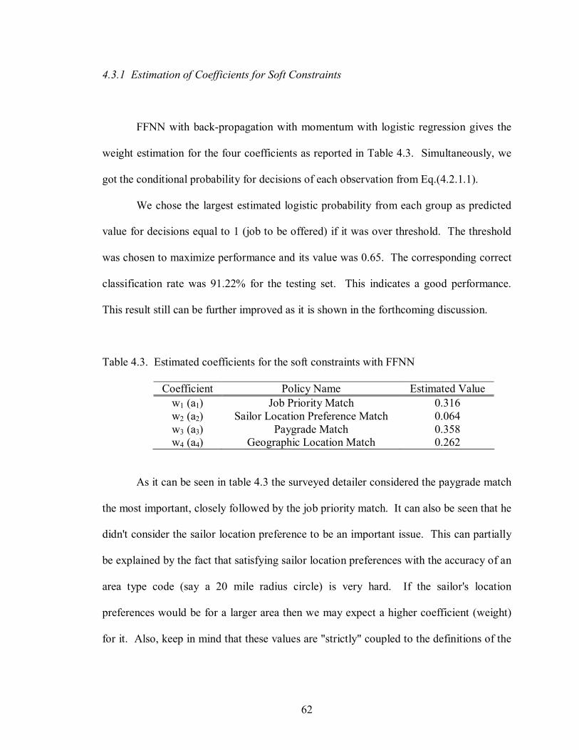
62

4.3.1 Estimation of Coefficients for Soft Constraints

FFNN with back­propagation with momentum with logistic regression gives the

weight estimation for the four coefficients as reported in Table 4.3. Simultaneously, we

got the conditional probability for decisions of each observation from Eq.(4.2.1.1).

We chose the largest estimated logistic probability from each group as predicted

value for decisions equal to 1 (job to be offered) if it was over threshold. The threshold

was chosen to maximize performance and its value was 0.65. The corresponding correct

classification rate was 91.22% for the testing set. This indicates a good performance.

This result still can be further improved as it is shown in the forthcoming discussion.

Table 4.3. Estimated coefficients for the soft constraints with FFNN

Coefficient Policy Name Estimated Value w1 (a1) Job Priority Match 0.316 w2 (a2) Sailor Location Preference Match 0.064 w3 (a3) Paygrade Match 0.358 w4 (a4) Geographic Location Match 0.262

As it can be seen in table 4.3 the surveyed detailer considered the paygrade match

the most important, closely followed by the job priority match. It can also be seen that he

didn't consider the sailor location preference to be an important issue. This can partially

be explained by the fact that satisfying sailor location preferences with the accuracy of an

area type code (say a 20 mile radius circle) is very hard. If the sailor's location

preferences would be for a larger area then we may expect a higher coefficient (weight)

for it. Also, keep in mind that these values are "strictly" coupled to the definitions of the

63

fi functions. A low value of a coefficient indicates high function values for cases when a

constraint is satisfied, and low values when it is not.

4.3.2 Neural Network for Decision Making

Multilayer Perceptron with one hidden layer was tested using tansig and logsig

activation functions for hidden and output layers respectively. Other activation functions

were also used but did not perform as well. MLP with two hidden layers were also tested

but no significant improvement was observed. Four different learning algorithms were

applied for sensitivity analysis.

Training was confined to 5000 epochs, but in most cases there were no significant

improvement in the MSE after 1000 epochs. The best MLP was obtained through

structural learning where the number of hidden nodes ranged from 2 to 20, while the

training set size was setup as 50%, 60%, 70%, 80%, and 90% of the sample set. The

cross­validation and testing sets each took the half of the rest. For the penalty factor λ

0.1 was used, which gave better generalization performance then other values for the data

set.

Using MDL criteria we can find out the best match of percentage of training with

the number of hidden nodes in a factorial array.

Table 4.4 reports MDL/AIC values for given number of hidden nodes and given

testing set sizes. As shown in the table, for 2, 5, and 7 nodes, 5% for testing, 5% for

cross validation, and 90% for training provides the lowest MDL. For 9 nodes the lowest

MDL was found for 10% testing, 10% cross validation, and 80% training set sizes. For

64

10­11 nodes the best MDL was reported for 20% cross­validation, 20% testing, and 60%

training set sizes. For 12­20 nodes the best size for testing set was 25%. We observe that

by increasing the number of hidden nodes the size of the training set should be increased

in order to lower the MDL and the AIC. Since MDL includes the size of the input

examples, which guides to the best partition of the data for cases when the MDL and AIC

values do not agree MDL is preferred.

Table 4.4. Factorial array for model selection for MLP with structural learning with

correlated group data: values of MDL and AIC up to 1000 epochs, according to Eqs.

(4.2.2.4) and (4.2.2.5)

# hidden nodes Size of testing set H 5% 10% 15% 20% 25% 2 ­57.2/­58.3 ­89.9/­96.3 ­172.3/181.7 ­159.6/­171.1 ­245.3/­258.5 5 ­12.7/­15.3 ­59.5/­74.7 ­116.4/­138.9 ­96.5/­124.3 ­188.0/­219.7 7 13.9/10.3 ­48.9/­27.8 ­93.5/­62.2 ­62.3/­100.9 ­161.0/­116.9 9 46.0/41.5 7.4/­21.6 ­22.1/­62.2 ­15.1/­64.4 ­91.7/­148.1 10 53.7/48.6 ­15.1/­64.4 63.4/19.0 10.3/­41.9 ­64.9/­127.6 11 70.1/64.5 41.1/8.3 152.4/103.6 29.2/­30.8 ­52.4/­121.2 12 85.6/79.5 60.5/24.6 39.9/­13.2 44.5/­21.0 ­27.7/­102.7 13 99.7/93.1 73.4/34.5 66.0/8.4 80.8/9.9 ­14.2/­95.4 14 120.4/113.3 90.8/49.0 86.6/24.6 101.4/25.1 20.8/­67.6 15 131.5/123.9 107.0/62.7 95.6/29.2 113.9/32.2 38.5/­58.4 17 166.6/158.0 138.0/87.4 182.4/107.2 149.4/56.9 62.2/­26.6 19 191.2/181.7 181.5/124.9 166.1/109.5 185.8/82.6 124.0/5.7 20 201.2/191.1 186.6/127.1 231.3/143.0 193.2/84.5 137.2/12.8

Table 4.5 provides the correlation coefficients between inputs and outputs for best

splitting of the data with given number of hidden nodes. 12­20 hidden nodes with 50%

training set provides higher values of the correlation coefficient than other cases. Figure

4.1 gives the average of the correct classification rates of 10 runs, given different

65

numbers of hidden nodes assuming the best splitting of data. The dotted line shows

results with different number of hidden nodes using structural learning. The solid line

shows results of Logistic regression projected out for comparison. The results were

consistent with table 4.4 and table 4.5. The 0.81 value of the correlation coefficient

shows that the network is reasonably good.

Table 4.5. Correlation Coefficients of inputs with outputs for MLP

Number of Hidden Nodes Correlation Coefficient Size of training set 2 0.7017 90% 5 0.7016 90% 7 0.7126 90% 9 0.7399 80% 10 0.7973 60% 11 0.8010 60% 12 0.8093 50% 13 0.8088 50% 14 0.8107 50% 15 0.8133 50% 17 0.8148 50% 19 0.8150 50% 20 0.8148 50%

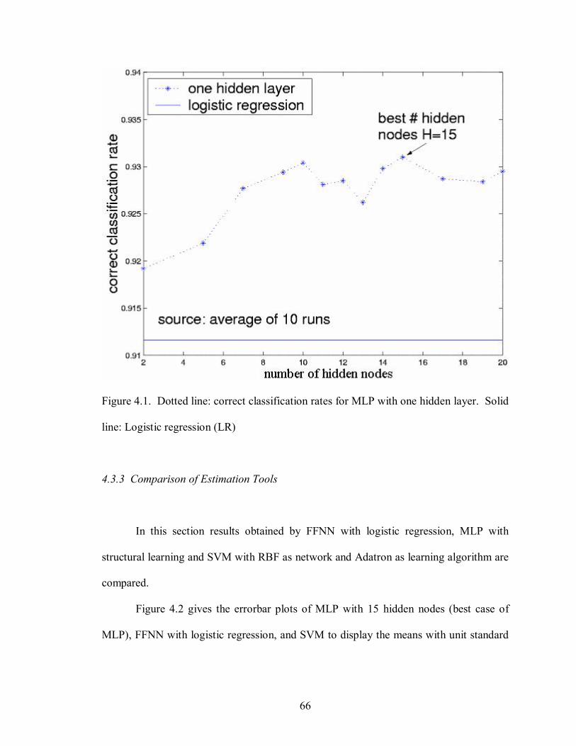
66

Figure 4.1. Dotted line: correct classification rates for MLP with one hidden layer. Solid

line: Logistic regression (LR)

4.3.3 Comparison of Estimation Tools

In this section results obtained by FFNN with logistic regression, MLP with

structural learning and SVM with RBF as network and Adatron as learning algorithm are

compared.

Figure 4.2 gives the errorbar plots of MLP with 15 hidden nodes (best case of

MLP), FFNN with logistic regression, and SVM to display the means with unit standard

67

deviation and medians for different size of testing samples. It shows how the size of the

testing set affects the correct classification rates for three different methods. As shown in

the figure the standard deviations are small for 5%­25% testing set sizes for the MLP.

The median and the mean are close to one another for 25% testing set size for all the

three methods, so taking the mean as the measurement of simulation error for these cases

is as robust as the median. Therefore the classification rates given in Figure 4.1 taking

the average of different runs as measurement is reasonable for our data. For cases when

the median is far from the mean, the median could be more robust statistical

measurement than the mean. The best MLP network from structural learning as it can be

seen in Figure 4.1 and Figure 4.2 is 15 nodes in the hidden layer and 25% testing set size.

Early stopping techniques were employed to avoid overfitting and to better the

generalization performance. Figure 4.3 shows the MSE of the training and the cross­

validation data with the best MLP with 15 hidden nodes and 50% training set size. The

MSE of the training data goes down below 0.09 and the cross­validation data started to

significantly increase after 700 epochs, therefore we use 700 for future models. Figure

4.4 shows the sensitivity analysis and the performance comparison of back­propagation

with momentum, conjugate gradient descent, quickprop, and delta­delta learning

algorithms for MLP with different number of hidden nodes and best cutting of the sample

set. As it can be seen their performance were relatively close for our data set, and delta­

delta performed the best. MLP with back­propagation with momentum also performed

well around 15 hidden nodes. MLP with 15 hidden nodes and 25% testing set size gave

approximately 6% error rate, which is a very good generalization performance for

68

predicting jobs to be offered for sailors. Even though SVM provided slightly higher

correct classification rate than MLP, it has a significant time complexity.

Some noise is naturally present when humans make decisions in a limited time

frame. Remember, that up to 20% difference could occur in the decisions even if the

same data would be presented to the same detailer at a different time and different

detailers are likely to make different decisions even under the same circumstances.

Moreover environmental changes might further bias decisions.

Figure 4.2. Errorbar plots with means (circle) with unit standard deviations and medians

(star) of the correct classification rates for MLP with one hidden layer (H = 15), Logistic

Regression (LR), and SVM

69

Figure 4.3. Typical MSE of training (dotted line) and cross­validation (solid line) with

the best MLP with one hidden layer

70

Figure 4.4. Performance of different training algorithms. Dotted line: Back­propagation

with Momentum, Dash­dotted line: Conjugate Gradient descent, Dashed line: Quickprop,

Solid line: Delta­Delta algorithm

4.4 Conclusion

High­quality decision making using optimum constraint satisfaction is an

important goal of IDA, to aid the Navy to achieve the best possible sailor and Navy

satisfaction performance. A number of neural networks with statistical criteria were

applied to either improve the performance of the current way IDA handles constraint

71

satisfaction or to come up with alternatives. IDA's constraint satisfaction module, neural

networks and traditional statistical methods are complementary with one another. It has

been shown by Kozma, Harter, and Achunala (2002) that constraint satisfaction plays the

primary role in action selection and therefore in intelligence. In this study we have

further learned that to achieve a good general model of human behavior and decision

making in an artificial intelligent system constraint satisfaction, machine learning, and

statistical assessment have to be assembled automatically (within the intelligent system).

We have also learned that intelligent behavior and decision making in an intelligent

system can be increased through adaptation to environmental changes and the right data

has to be provided to be used as training data in sufficient quantity and frequency.

Having learned all these about artificial intelligent systems we can build a theory that

constraint satisfaction, learning, and statistical assessment have to be integrated

automatically for human intelligence. Also it can be safely said that high level human

intelligence requires adaptation to environmental changes and efficient training data has

to be provided in sufficient quantity and frequency.

In this chapter we combined MLP with structural learning and statistical criteria,

which provided us with the best MLP with one hidden layer for decision classification

and a good candidate to replace the linear functional in IDA. Fifteen hidden nodes and

25% testing set size using back­propagation with momentum and delta­delta learning

algorithms provided good generalization performance for the used data set. SVM with

RBF network architecture and Adatron learning algorithm gave the best prediction

performance for decision classification with an error rate below 6%, although with

72

significant time cost. In comparison to human detailers such a performance is

remarkable.

Coefficients for the existing IDA constraint satisfaction module were also adapted

via FFNN with logistic regression. It is important to keep in mind that the coefficients

have to be updated from time to time as well as online neural network trainings are

necessary to comply with changing Navy policies and other environmental challenges.

The possible inclusion of neural networks as an external module (a module which would

run in parallel with IDA providing coefficients to IDA automatically, periodically) for

IDA can spare the intelligent agent's architecture from growing more complex, while

efficiently assisting the constraint satisfaction module to keep pace with the changing

demands posed by the environment. Although such integration is not part of this

dissertation. Decision on what further changes IDA needs have to be evaluated carefully

with the cooperation of other IDA developers and researchers. If we choose to replace

the current linear functional module for constraint satisfaction with a neural network, that

may clearly model human cognition, decision making, and learning far better with its

own infamous black­box nature. Neural networks, particularly support vector machines

are well suited to decision making tasks in noisy, ever changing, and self contradicting

environment and data.

Having seen how neural networks can be utilized to augment the decision making

process in IDA in the next section we turn to investigate a model, which combines

benefits of neural networks and fuzzy systems. The method is known as Adaptive

Neuro­Fuzzy Inference System and is able to provide more explanation about decisions

once the training has been completed in the form of fuzzy rules.

73

5 Adaptive Neuro­Fuzzy Inference System

Applying a neuro­fuzzy inference system to model the decision making problem

is quite natural, because of the similarity to real life human decision­making. In this

chapter as an alternative to the current IDA linear functional approach for decision­

making support an Adaptive Neuro­Fuzzy Inference System (ANFIS) is discussed. The

system can learn to make human­like decisions and uses fuzzy membership functions for

soft constraints to reflect satisfaction degrees. The goal is to find the most appropriate

control actions (decisions resulting from fuzzy rules) for matches between jobs and

sailors. Further goal is to extract a small number of fuzzy rules, which are still very

effective without giving up robustness.

Once initial training of the system is done, it could be integrated into IDA, which

would enable it to learn even further. It may adapt to environmental changes (such as

economic change, Navy policy change, wartime/peacetime change, etc.), unseen

situations, and increase efficiency. Moreover with periodic use of data coming from

human detailers, the system may learn to make better and up to date human­like

decisions, which can also follow environmental changes with some delay.

Even though human detailers may face some difficulties in defining real valued

functions and numeric coefficients to be applied in IDA’s current linear functional model,

the use of fuzzy membership functions and values is convenient, because detailers can

easily express their decisions in terms of linguistic descriptions (such as high, medium,

low) in regard to constraints as well as to the overall fitness of the match between sailors

and jobs.

74

For data acquisition and preprocessing the method discussed in subsection 4.1

was used, which is summarized below with some modifications. The used Navy

databases contained 467 sailors and 167 possible jobs for them. The data first was pre­

processed and cleaned, eliminating unnecessary and superfluous attributes. This resulted

with 18 attributes from the sailor database and 6 from the job database. Hard constraints

then were employed to filter away the inappropriate “matches” between sailors and jobs.

On the 1277 matches that passed the hard constraints, the soft constraints were applied,

then their values were fuzzified. These values served as inputs to the neuro­fuzzy

inference system. The used soft constraints were the same as before: Job Priority Match,

Sailor Location Preference Match, Paygrade Match (soft), Geographic Location Match,

each of which were represented by a monotone function. Output data (decisions) were

acquired from a detailer in the form of Boolean answers for each possible match and he

was asked to make decisions based only on the discussed soft constraints. Decisions

were made sequentially and independently.

Every sailor along with all his/her possible jobs that satisfy the hard constraints

were assigned to a unique group, which is called group ID. The numbers of jobs in each

group were counted and normalized to fit the [0,1] unit interval by simply dividing them

by the maximum value; this will be used later for decision refinement. In some

experiments they were included in the input as function f5.

75

5.1 Design of Adaptive Neuro­Fuzzy Inference System

Some design issues were set up based on information from Navy experts, while

others were learned. IDA’s current real valued satisfaction degrees (f1,...,f4 values) for

soft constraints were fuzzified for initial training of the Adaptive Neuro­Fuzzy Inference

System. Later on linguistic descriptions such as low, medium, high from human detailers

can be used. Even though fuzzification may mean some initial loss of information

already included in the f1,...,f4 functions, the difficulty of frequent, delicate tuning of

those over time as the environment changes can be reduced. Some of the design issues of

the ANFIS were the following:

1. Number of input membership functions: the fuzzy membership functions were

set up based on knowledge on detailer decisions. It was determined that three

membership functions (low, medium, high) for each of the four soft constraints model

detailer decisions well. Two and five membership functions were also tested.

2. Type of input membership functions: based on the properties of the soft

constraints we primarily consider triangular membership functions, yet trapezoid,

Gaussian curve and generalized bell­shaped membership functions were tested as well.

3. Type of output membership functions: a single output, obtained using weighted

average defuzzification was used. All output membership functions had the same type

and were either constant or linear (zeroth and first order Sugeno type system).

4. The number of output membership functions: it ranged from 2 to 243.

76

5. The number of rules: for a well defined fuzzy system it is necessary to define

control actions (fuzzy output) for every possible combination of input membership

function values. If the training set doesn’t include examples for a given combination of

values, but the testing set does then in the testing phase the output value can be "guessed"

using the aggregate distance function from all the learned fuzzy rules. This can be done

before the actual testing phase begins resulting in a fully defined fuzzy system. In our

case four constraints, each with three membership functions result in 3 4 (81) fuzzy rules,

where the linguistic values were not negated, and they were connected with “and”

relation. In some of the experiments 5 inputs were used, each with 3 membership

functions, which result in 3 5 (243) fuzzy rules with the same assumptions as above.

However, through rule extraction and combination of rules the number of rules can be

drastically reduced later.

6. Performance function: some of the widely used performance functions in neural

networks are Sum of Squared Error, Mean Squared Error, and cost function given in

Eq.(4.2.2.2) (Ishikawa, 1996; Kozma, Sakuma, Yokoyama, & Kitamura, 1996). To

verify training performance the correct classification rate can also be verified.

7. Optimization methods: back­propagation and hybrid (mixed least squares and

backpropagation) methods had been used as optimization methods.

8. Partitioning the data into training, cross­validation and testing sets: the range of

the training data set size was 50% to 90%. The cross­validation and testing data sets each

took half of the rest of the data (5%­25%). The use of cross­validation is optional but in

our implementation is important, to avoid overtraining.

9. Number of epochs: in most runs it was set up to 500.

77

Through an adaptive neuro­fuzzy inference system the range of the membership

functions are learned, a set of fuzzy rules are created and their weights are adjusted in

order to better model the training data. The performance function values are calculated,

and classification is provided.

5.2 Results and Rule Extraction

For implementation Matlab 6.1 environment with fuzzy logic toolbox was used.

Various types of input membership functions have been tested, and as we expected the

triangular membership functions performed best closely followed by trapezoid, Gaussian

curve and generalized bell­shaped membership functions.

Linear output membership functions performed better than constant ones.

For optimization method the back­propagation and hybrid optimization method

performed similarly regarding the performance function and classification, but the hybrid

method's running time was about five times as long as that of the backpropagation’s.

To avoid overtraining cross­validation was used. In some cases the minimum

cross­validation error occurred within the first epoch. This meant that the given set of

membership functions were not a good choice for modeling the training data. This also

indicated that either more data needed to be selected for training, or a modification of the

membership functions (both the number of membership functions and their types) was

necessary. After training, the FIS parameters were set to be associated with the minimum

cross­validation error.

78

Figure 5.1 shows the generated ANFIS model structure. Its layered structure from

left to right is the following:

Layer 1. Input neurons: four input neurons for the four soft constraints.

Layer 2. Input membership functions: three triangular membership functions for

each input neuron

Layer 3. Fuzzy rule left­hand sides: each connected to 4 input membership

functions.

Layer 4. Output membership functions (right­hand sides): the right­hand side

rules are in one to one relation with the left­hand side rules.

Layer 5 Aggregated output: each output membership function gets aggregated

along with the weight they carry.

Layer 6. Output (decision).

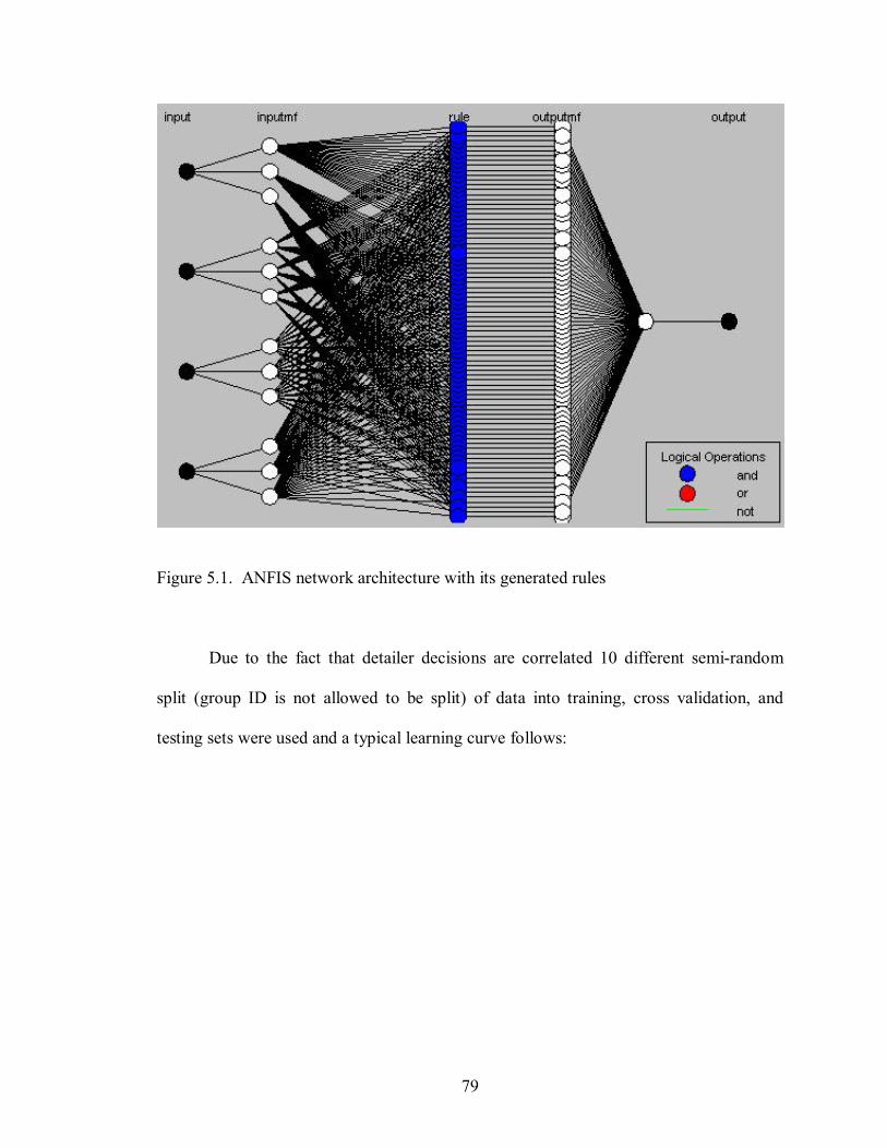
79

Figure 5.1. ANFIS network architecture with its generated rules

Due to the fact that detailer decisions are correlated 10 different semi­random

split (group ID is not allowed to be split) of data into training, cross validation, and

testing sets were used and a typical learning curve follows:

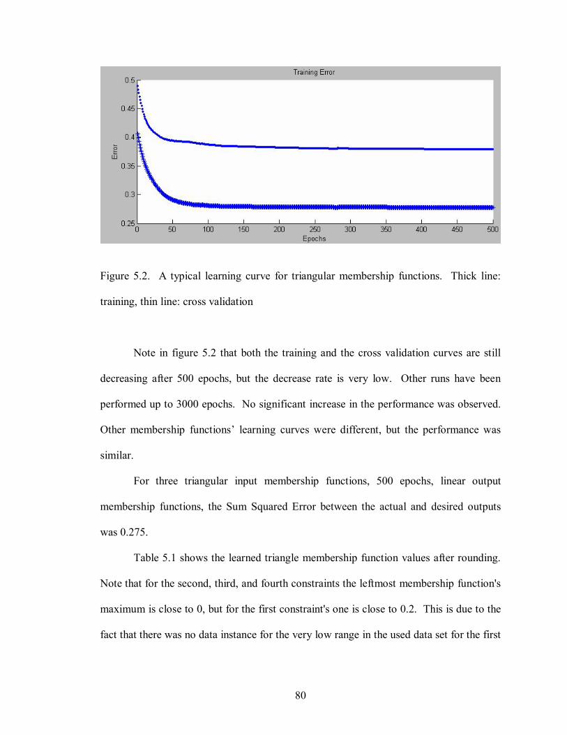
80

Figure 5.2. A typical learning curve for triangular membership functions. Thick line:

training, thin line: cross validation

Note in figure 5.2 that both the training and the cross validation curves are still

decreasing after 500 epochs, but the decrease rate is very low. Other runs have been

performed up to 3000 epochs. No significant increase in the performance was observed.

Other membership functions’ learning curves were different, but the performance was

similar.

For three triangular input membership functions, 500 epochs, linear output

membership functions, the Sum Squared Error between the actual and desired outputs

was 0.275.

Table 5.1 shows the learned triangle membership function values after rounding.

Note that for the second, third, and fourth constraints the leftmost membership function's

maximum is close to 0, but for the first constraint's one is close to 0.2. This is due to the

fact that there was no data instance for the very low range in the used data set for the first

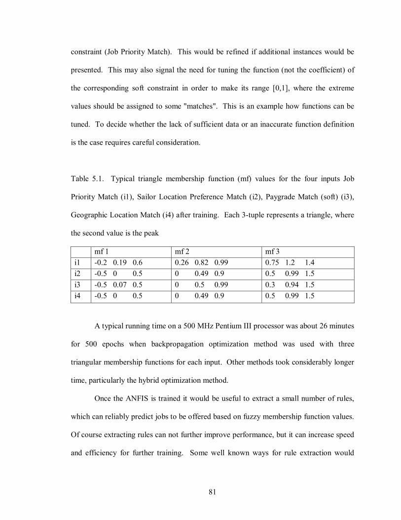
81

constraint (Job Priority Match). This would be refined if additional instances would be

presented. This may also signal the need for tuning the function (not the coefficient) of

the corresponding soft constraint in order to make its range [0,1], where the extreme

values should be assigned to some "matches". This is an example how functions can be

tuned. To decide whether the lack of sufficient data or an inaccurate function definition

is the case requires careful consideration.

Table 5.1. Typical triangle membership function (mf) values for the four inputs Job

Priority Match (i1), Sailor Location Preference Match (i2), Paygrade Match (soft) (i3),

Geographic Location Match (i4) after training. Each 3­tuple represents a triangle, where

the second value is the peak

mf 1 mf 2 mf 3 i1 ­0.2 0.19 0.6 0.26 0.82 0.99 0.75 1.2 1.4 i2 ­0.5 0 0.5 0 0.49 0.9 0.5 0.99 1.5 i3 ­0.5 0.07 0.5 0 0.5 0.99 0.3 0.94 1.5 i4 ­0.5 0 0.5 0 0.49 0.9 0.5 0.99 1.5

A typical running time on a 500 MHz Pentium III processor was about 26 minutes

for 500 epochs when backpropagation optimization method was used with three

triangular membership functions for each input. Other methods took considerably longer

time, particularly the hybrid optimization method.

Once the ANFIS is trained it would be useful to extract a small number of rules,

which can reliably predict jobs to be offered based on fuzzy membership function values.

Of course extracting rules can not further improve performance, but it can increase speed

and efficiency for further training. Some well known ways for rule extraction would

82

involve structural learning or genetic algorithms. Yet, we employed the Fast Apriori

algorithm, which applies the association rule data mining technique (Agrawal, Mannila,

Srikant, Toivonen, & Verkamo, 1996; Bayardo & Agrawal, 1999). Each association rule

is in a form of if then rules. In our case linguistic values for input and output

membership functions can predict each other. Of course we are only interested in rules,

which predict for output, such as: if all the four soft constraints are highly satisfied then

the output is high.

The algorithm was run after the training session. We setup support (percentage of

data that the given rule is applicable) and confidence (percentage that the rule holds if it

is applicable) thresholds for rule extraction. We commonly used 1% support, 50%

confidence. This means that we are only interested in rules that are true in more than

50% of the time, and rules that are applicable on at least 1% of the data.

In the case of four inputs, each with three triangular membership functions with

70% training data and back­propagation optimization method there were 81 fuzzy rules

learned by the ANFIS system. Also with the Fast Apriori algorithm with 1% support and

50% confidence 448 "mined" rules were extracted, but only 111 predicted for decision.

Note that "mined" rules and fuzzy rules are different. See examples for "mined" rules in

table 5.2, and for fuzzy rules in table 5.3. There were 12 "mined" rules to predict positive

decisions, but 4 of them were “not interesting”. As it can be seen in Table 5.2 they

predicted with low/medium values for some inputs and there were corresponding

stronger, more important rules. The “not interesting” rules are marked with *, and they

were eliminated.

83

After extracting the 8 positive rules a minimal number of negative rules are

created in order to cover all possible input combinations. This can be done by negating

the disjunction of the 8 positive rules and transforming them to a complete disjunctive

normal form, then cutting that form at the disjunctions points into new rules. Applying

this technique 4 new rules were generated. Table 5.3 shows the 12 final rules, where the

first 8 are the positive rules and the rest are the negative rules.

Table 5.2. Extracted "mined" rules through fast Apriori algorithm. 2,5,8,11 mean high

values for inputs 1,2,3,4, respectively. 12 means positive decision. Other occurring

values mean low and medium values for inputs 1,…,4. Numbers in parenthesis: support

and confidence. Rules with * were dropped

12 <­ "8 2 (21.4%, 53.9%)"

12 <­ "8 11 (7.6%, 54.4%)"

12 <­ "8 5 (5.7%, 51.0%)"

*12 <­ "3 8 2 (18.7%, 50.3%)"

*12 <­ "3 8 11 (5.6%, 52.0%)"

12 <­ "8 2 11 (3.9%, 80.0%)"

12 <­ "8 2 5 (2.7%, 79.2%)"

12 <­ "8 11 5 (2.0%, 61.1%)"

12 <­ "2 11 5 (2.5%, 54.5%)"

*12 <­ "3 8 2 11 (2.8%, 76.0%)"

*12 <­ "9 8 2 5 (1.6%, 71.4%)"

12 <­ "8 2 11 5 (1.1%, 90.0%)"

84

Table 5.3. Fuzzy rules after rule extraction. The numbered output values can help to

trace decisions made by ANFIS, but from the decision making point of view are

irrelevant. i1 = Job priority, i2 = Sailor location preference, i3 = Paygrade, i4 =

Geographic location

1. If (i1 is high) and (i3 is high) then (o is high1)

2. If (i3 is high) and (i4 is high) then (o is high2)

3. If (i2 is high) and (i3 is high) then (o is high3)

4. If (i1 is high) and (i3 is high) and (i4 is high) then (o is high4)

5. If (i1 is high) and (i2 is high) and (i3 is high) then (o is high5)

6. If (i2 is high) and (i3 is high) and (i4 is high) then (o is high6)

7. If (i1 is high) and (i2 is high) and (i4 is high) then (o is high7)

8. If (i1 is high) and (i2 is high) and (i3 is high) and (i4 is high) then (o is high8)

9. If (i1 is not high) and (i2 is not high) and (i4 is not high) the (o is low1)

10. If (i1 is not high) and (i3 is not high) the (o is low2)

11. If (i2 is not high) and (i3 is not high) the (o is low3)

12. If (i3 is not high) and (i4 is not high) the (o is low4)

Naturally, we might extract different rules with different supports and

confidences. We can also further extract rules, because some of them are stronger than

others. Rules 4,5,6,8 can be extracted this way. However, we chose not to do so because

these rules are fuzzy rules, not sharp ones. Of course with the same argument we may

also keep the 4 dropped rules from Table 5.2.

85

The next task is to feed back the extracted rules to the ANFIS and see how much

it decreased the performance. The average of 10 runs show that it decreased the correct

classification rate by only about 1%, which means that the rule extraction was efficient.

Figure 5.3 shows the structure of the ANFIS after rule extraction. As it can be

seen in figure 5.4 the testing results after rule extraction provided approximately 92%

correct classification rate. The optimal decision threshold was chosen from training

results, and its value was 0.41. We can also see that the classification rate for “denied”

decisions was about 96%, and 70% for “offered” ones. Due to the fact that there were far

too more “denied” decisions than “offered” ones, the correct classification rate for

“denied” decisions was far higher than that of “offered” decisions.

Figure 5.5 and figure 5.6 show some of the learned surfaces after rule extraction.

Figure 5.3. ANFIS network architecture after rule extraction.

86

Figure 5.4. Testing results (190 samples) after rule extraction. Blue line: desired output

(0 for negative, 1 for positive decisions). Red stars: network output (prediction).

Decision threshold: 0.41

Figure 5.5. Learned surface plot on input 1 and input 2

87

Figure 5.5 shows that input 1 and input 2 are approximately equally important for

positive decisions. On the contrary, according to figure 5.6, input 3 contributes to

positive decisions better than input 1. We can also see that the number of positive

decisions suddenly increase when both inputs provide high values.

To further improve the classification rates we applied our extra knowledge about

the data set: Detailers typically offer exactly one job to sailors. Offering only a job with

the highest output value could greatly increase the classification rate. This was the

reason that we didn’t allow group ID’s to be split into different partition (training, cross­

validation, testing). Using this method the classification rate increased to up to 93.2%.

Figure 5.6. Learned surface plot on input 1 and input 3

88

Decisions for jobs to be offered have been individually evaluated for the best

result of the model and it was determined that even the misclassified predictions would

make sense as real human like decisions based on the given soft constraints. In some of

the experiments the number of jobs were included as an additional input with fuzzified

values, and it yielded about 93% classification rate.

5.3 Forming Hypothesis on Detailer Decisions

The Application of the above Adaptive Neuro­Fuzzy Inference System for

learning fuzzy rules and the fast Apriori algorithm for rule extraction enables us to build

a model or hypothesis on how humans, in particular human detailers make decisions for

constraint satisfaction problems. This may allow us to “see into the detailers’ mind” and

build cognitive models on human constraint satisfaction, decision making, learning and

intelligence.

Humans are faced with constraint satisfaction problems multiple times every day.

Constraints can be hard and soft, similarly to the domain we have discussed so far and

which detailers face. It is easy to hypothesize that decisions to satisfy hard constraints

are actually made in terms of rules. For example a student initially may not know that “if

he doesn’t do his homework then he will get a bad grade”. After he experiences a bad

grade he may modify the old rule “if there is homework then do nothing” to “if there is

homework then do it”. This new rule will be applied to the next situation, which may

result a better grade so the new rule gets reinforced and applied in future situations,

89

unless other stronger and contradictory rules are created for some reason. Rules get

reinforced if they work in a new situation. Otherwise they get weakened, modified or

even discarded.

The agent’s (humans') long­term goal could be to produce a short list of robust

rules, which can apply to any situation the agent may face in the future. We can also

build a hypothesis that for constraint satisfaction problems, where the constraints are soft,

decision making can be done similarly. In humans, the selection of a rule or rules to be

applied happens with the help of long term memory. In our discussed system (IDA with

a smart constraint satisfaction module, perhaps with an Adaptive Neuro­Fuzzy Inference

System) rules should be chosen based on statistical frequency (which is similar to human

long­term memory) and simplicity (Occam’s razor).

Using all the domain specific knowledge on detailer decisions and the results

obtained via the method discussed in this chapter we have built a hypothesis that a

detailer makes decisions in the following steps:

1. Get all relevant data about a sailor in question.

2. Apply rules to satisfy hard constraints (Bring up all applicable jobs for the

sailor).

3. Assign three level (low, medium high) linguistic values for those soft

constraints, which the detailer considers important (the surveyed detailer

considered the following important: Job Priority, Sailor Location Preference,

Paygrade, Geographic Location).

4. Apply rules from top to down (based on Table 5.4) to each job and make

temporary decisions (offer or deny job) based on the first applicable rule.

90

5. Change each decision from “offer” to “deny”, if there is a corresponding

“offer” decision obtained via the application of a more important rule. (Keep

only those “offer” decisions, which are a result of the highest applicable rule.)

6. If the highest applicable rule can be applied to one job only then mark the

corresponding job to be offered.

7. If the highest applicable rule is applicable to more than one job then apply

tiebreaker (look at the actual data for the most important soft constraint). (The

surveyed detailer looked at Job Priority). If the tiebreaker does not provide a

strong break then mark two, or even three jobs to be offered. (According to

the surveyed detailer, a minimum of 3 difference in job priority was

considered a strong tiebreak.)

8. If there is no applicable rule to offer job for the sailor then mark no jobs to be

offered.

9. Stop decision making process.

Table 5.4. Rules to be used by detailers on soft constraints in order (highest first). To fit

the above algorithm only those rules are listed, which provide positive (“offer”)

decisions. i1 = Job Priority, i2 = Sailor Location Preference, i3 = Paygrade, i4 =

Geographic Location , o = output.

1. If (i1 is high) and (i2 is high) and (i3 is high) and (i4 is high) then (o is high)

2. If (i1 is high) and (i3 is high) and (i4 is high) then (o is high)

3. If (i1 is high) and (i2 is high) and (i3 is high) then (o is high)

4. If (i2 is high) and (i3 is high) and (i4 is high) then (o is high)

91

5. If (i1 is high) and (i2 is high) and (i4 is high) then (o is high)

6. If (i3 is high) and (i4 is high) then (o is high)

7. If (i1 is high) and (i3 is high) then (o is high)

8. If (i2 is high) and (i3 is high) then (o is high)

Table 5.5. Rules to be used by detailers on soft constraints in linguistic terms in order

(highest first).

1. If (Job Priority is high) and (Sailor Location Preference is high) and (Paygrade

is high) and (Geographic Location is high) then (offer job)

2. If (Job Priority is high) and (Paygrade is high) and (Geographic Location is

high) then (offer job)

3. If (Job Priority is high) and (Sailor Location Preference is high) and (Paygrade

is high) then (offer job)

4. If (Sailor Location Preference is high) and (Paygrade is high) and (Geographic

Location is high) then (offer job)

5. If (Job Priority is high) and (Sailor Location Preference is high) and

(Geographic Location is high) then (offer job)

6. If (Paygrade is high) and (Geographic Location is high) then (offer job)

7. If (Job Priority is high) and (Paygrade is high) then (offer job)

8. If (Sailor Location Preference is high) and (Paygrade is high) then (offer job)

Table 5.5 lists the same rules as table 5.4, but in linguistic terms. We can further

hypothesize that these rules are really fuzzy for detailers. For example a value of 8 for

92

Job priority may sometimes be considered high and other times medium. The

corresponding decisions (what is high and what is not) or “membership functions” get

adjusted via learning and experience with the data. It is adjusted based on short­term

memory and long term memory. Short­term memory is used to perform fine adjustment

on what values correspond to a high match for a soft constraint based on the particular

data the detailer is working with for the particular sailor. Long­term memory is used to

perform a more permanent change in what a detailers considers a high match for a soft

constraint in general.

Based on all the results of this chapter we can further hypothesize that the

surveyed detailer considered Paygrade (i3) the most important soft constraint, followed

by Job Priority (i1), then Geographic Location (i4), and finally Sailor Location

Preference (i2).

5.4 Offering Multiple Jobs to Sailors

Due to the fact that we use fuzzy membership functions and that sometimes two

or more jobs could equally or nearly equally satisfy the given soft constraints the highest

value may not be easily available. In this case we would prefer to come up with a small

set (with 1 to 4 elements) of possible jobs for the given sailor. In fact this is a desirable

property according to recent feedback from Navy experts, which states that ideally a

detailer should offer three jobs to sailors to choose from.

93

5.5 Conclusion

In this chapter an Adaptive Neuro­Fuzzy Inference System was discussed as a

possible substitute for IDA's current linear functional module. Design, implementation

and testing of ANFIS based on data available to IDA has been completed, but integration

with IDA is not part of the dissertation. Results show that human like­decisions can be

achieved with the model. With the help of association rules a handful of fuzzy rules were

obtained, which have nearly as good performance as the original set of rules trained by

the ANFIS for decision making. Due to current Navy practices and real world constraints

periodic training of this system is necessary to keep pace with the ever­evolving

environmental challenges.

An Adaptive Neuro­Fuzzy Inference System has many benefits and some

drawbacks. It is very suitable to our data and surveys of Navy experts and others can

happen in terms of linguistic descriptions, which is convenient and helps to decrease the

noise coming from detailer decisions. Also, instead of tuning the coefficients ANFIS

would learn online, and follow detailer decisions. On the other hand, the decision

classification accuracy can be surpassed with other methods and it is computationally

expensive. However, the goal of approximating detailer decisions is expected to

eventually shift to a more objective evaluation criteria, which would include sailor

feedback. Also, new training of the ANFIS may only be necessary periodically, probably

once in every two or more weeks, which is well within the module's capability. Once the

training is completed decisions can be made in the fraction of a second.

94

For cognitive modeling ANFIS not only bears the benefits of neural networks, but

also able to generate rules, which are somewhat similar to what humans do: using all the

knowledge acquired via experience they generate rules, which can be applied to a wide

range of situations. If a new experience contradicts the expectation then the rules are

updated. The issue whether those rules are fuzzy is arguable.

This completes our tour of neural networks as a support for decision making. In

the next section we discuss an innovative a method, called Adaptive Generalized

Estimation Equation with Bayes Classifier, which combines advanced statistical tools

with data mining techniques. It is an extension of Bayesian networks and is able provide

high quality decision approximation and can learn coefficients more efficiently for the

existing linear functional model.

95

6 Adaptive Generalized Estimation Equation with Bayes Classifier

In this chapter an Adaptive Generalized Estimation Equation (AGEE) with

additive noise model is designed and discussed to model the constraints satisfaction of

IDA. This model can provide high level decision classification, so it can be used as a

substitute for IDA's linear functional. Also as a side effect it provides good estimates for

coefficients, which can be used in IDA's current linear functional module. The AGEE

models can be directly used to estimate the effects of the changes over time in covariates

(values of f1,...,f4) on the decision (job to be offered) with the correlated data (provided

by the survey of detailers) and give us more insight into what criteria are important to

decision­makers and the weight of each. To handle the noise (coming from the

subjective and indeterminate nature of human decisions or dependency on the state of the

environment, etc.) and the outlier data (decisions made in error or due to some unknown

cause), we use Gibbs sampling under Bayesian framework with some prior information

(to know which sample belong to positive and which to negative decisions) (Gelfand,

Hills, Racine­Poon, & Smith, 1990; Albert & Jais, 1998; Spiegelman, Rosner & Logan,

2000). Based on the estimations of AGEE with additive noise model, Adaptive Bayes

(AB) classifiers are proposed which use a modified Naive Bayes algorithm (Keller,

Schummer, Hood, & Ruzzo, 2000) for classification and prediction. In this chapter we

show how to combine advanced statistical approaches with data mining techniques

through using data from human detailers to build new classifiers to enhance the

performance of the job­assignment process.

96

As we have seen in chapter 4 and chapter 5 the data was taken from Navy

databases and from surveys of Navy experts. The databases contained data about 467

sailors and 167 possible jobs for them. The data was pre­processed and cleaned,

eliminating unnecessary and superfluous attributes. This resulted with 18 attributes from

the sailor database and 6 from the job database. Then the hard constraints were applied

to filter away the inappropriate “matches” between sailors and jobs. After that, the four

functions representing the soft constraints (Job Priority Match, Sailor Location

Preference Match, Soft Paygrade Match, Geographic Location Match) were applied.

Then the data is sent through the classification algorithm to build the model for

classification. We set aside one­third of the data for testing purpose, and based on the

test set we obtain the accuracy of the classifier.

6.1 Classification Model

6.1.1 GEE Model for Correlated Data

Generalized Estimation Equation (GEE) models were developed to extend the

Generalized Linear Models (GLM) to accommodate correlated data. It can be used to

estimate the effects of the changes over time in covariates Eq.(4.2.1.1) (values of f1,...,f4)

on the correlated surveyed decision and give us more insight into what criteria are

important to decision­makers and the weight of each. Generalized Estimation Equation

model was introduced by (Liang & Zeger, 1986). The marginal expectation (average

response for observations sharing the same covariates) is modeled as a logistic function

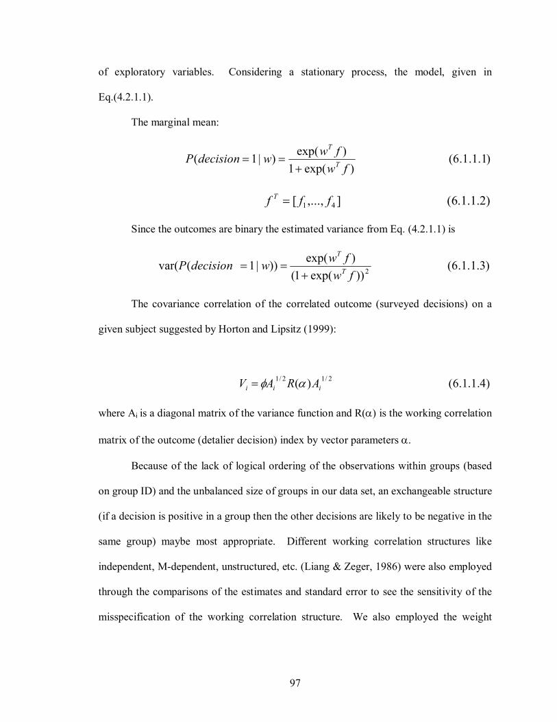
97

of exploratory variables. Considering a stationary process, the model, given in

Eq.(4.2.1.1).

The marginal mean:

) 1 . 1 . 1 . 6 ( ) exp( 1

) exp( ) | 1 ( f w f w w decision P T

T

+ = =

) 2 . 1 . 1 . 6 ( ] ,..., [ 4 1 f f f T =

Since the outcomes are binary the estimated variance from Eq. (4.2.1.1) is

) 3 . 1 . 1 . 6 ( )) exp( 1 ( ) exp( )) | 1 ( var( 2 f w f w w decision P T

T

+ = =

The covariance correlation of the correlated outcome (surveyed decisions) on a

given subject suggested by Horton and Lipsitz (1999):

) 4 . 1 . 1 . 6 ( ) ( 2 / 1 2 / 1 i i i A R A V α φ =

where Ai is a diagonal matrix of the variance function and R(α) is the working correlation

matrix of the outcome (detalier decision) index by vector parameters α.

Because of the lack of logical ordering of the observations within groups (based

on group ID) and the unbalanced size of groups in our data set, an exchangeable structure

(if a decision is positive in a group then the other decisions are likely to be negative in the

same group) maybe most appropriate. Different working correlation structures like

independent, M­dependent, unstructured, etc. (Liang & Zeger, 1986) were also employed

through the comparisons of the estimates and standard error to see the sensitivity of the

misspecification of the working correlation structure. We also employed the weight

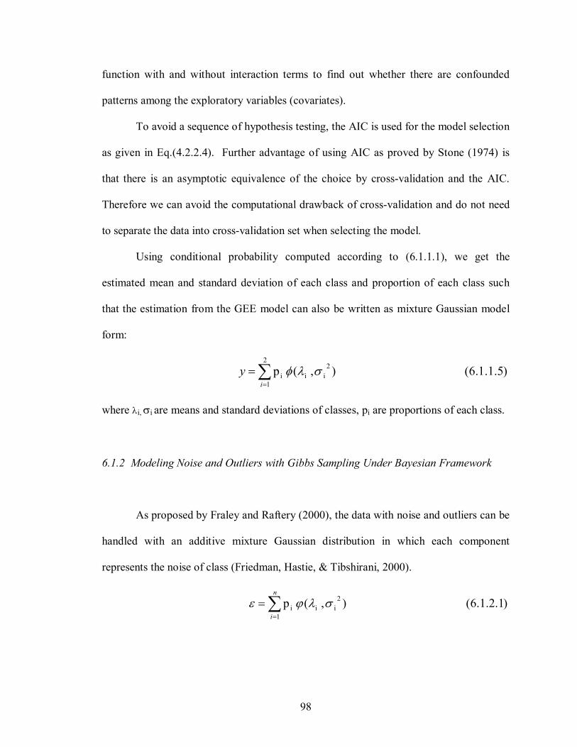
98

function with and without interaction terms to find out whether there are confounded

patterns among the exploratory variables (covariates).

To avoid a sequence of hypothesis testing, the AIC is used for the model selection

as given in Eq.(4.2.2.4). Further advantage of using AIC as proved by Stone (1974) is

that there is an asymptotic equivalence of the choice by cross­validation and the AIC.

Therefore we can avoid the computational drawback of cross­validation and do not need

to separate the data into cross­validation set when selecting the model.

Using conditional probability computed according to (6.1.1.1), we get the

estimated mean and standard deviation of each class and proportion of each class such

that the estimation from the GEE model can also be written as mixture Gaussian model

form:

) 5 . 1 . 1 . 6 ( ) , ( p 2i i

2

1 i σ λ φ ∑

=

= i

y

where λi, σi are means and standard deviations of classes, pi are proportions of each class.

6.1.2 Modeling Noise and Outliers with Gibbs Sampling Under Bayesian Framework

As proposed by Fraley and Raftery (2000), the data with noise and outliers can be

handled with an additive mixture Gaussian distribution in which each component

represents the noise of class (Friedman, Hastie, & Tibshirani, 2000).

) 1 . 2 . 1 . 6 ( ) , ( p 2i i

1 i σ λ ϕ ε ∑

=

= n

i

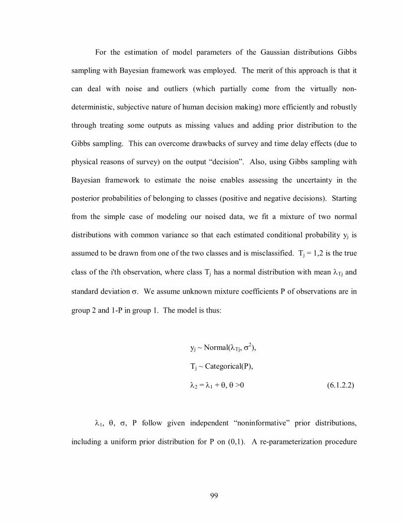
99

For the estimation of model parameters of the Gaussian distributions Gibbs

sampling with Bayesian framework was employed. The merit of this approach is that it

can deal with noise and outliers (which partially come from the virtually non­

deterministic, subjective nature of human decision making) more efficiently and robustly

through treating some outputs as missing values and adding prior distribution to the

Gibbs sampling. This can overcome drawbacks of survey and time delay effects (due to

physical reasons of survey) on the output “decision”. Also, using Gibbs sampling with

Bayesian framework to estimate the noise enables assessing the uncertainty in the

posterior probabilities of belonging to classes (positive and negative decisions). Starting

from the simple case of modeling our noised data, we fit a mixture of two normal

distributions with common variance so that each estimated conditional probability yj is

assumed to be drawn from one of the two classes and is misclassified. Tj = 1,2 is the true

class of the i'th observation, where class Tj has a normal distribution with mean λTj and

standard deviation σ. We assume unknown mixture coefficients P of observations are in

group 2 and 1­P in group 1. The model is thus:

yj ~ Normal(λTj, σ 2 ),

Tj ~ Categorical(P),

λ2 = λ1 + θ, θ >0 (6.1.2.2)

λ1, θ, σ, P follow given independent “noninformative” prior distributions,

including a uniform prior distribution for P on (0,1). A re­parameterization procedure

100

(estimation of λ1, θ, σ, P) was employed to avoid the data go to the same class through

shift λ2 with θ.

The equation (6.1.1.5) provides estimation of the parameters of two classes served

as initial values for Gibbs sampling under Bayesian framework, which can speed up the

convergence of Gibbs sampling. The prior distribution applied Dirichlet function.

6.1.3 Adaptive Bayes Classifiers and Algorithm for Correlated Data Combining GEE

with Additive Noise Model

The test class of the sample can be separate using likelihood and modified Naive

Bayes (NB) algorithm (Han & Kamber, 2000). The computed class of the model is the

model the sample has greatest likelihood

) 1 . 3 . 1 . 6 ( )) | ( max(log arg ) ( i i M x p x class =

The original NB algorithm uses the assumption of independence, which assumes

given the class model the value for each attributes are independent of one another, then

the class of the test sample can be given according to the following form:

) 2 . 3 . 1 . 6 ( ) | ( log max arg ) ( ∑ = k

i k

k i M x p x class

where k’s are attributes.

The modified NB classifier is directly based on the conditional probability

estimated from AGEE with additive model and (6.1.1.5). When substituting each class

for a Gaussian distribution with estimated mean λi and standard deviation σi. The test

sample of the class can be decided by

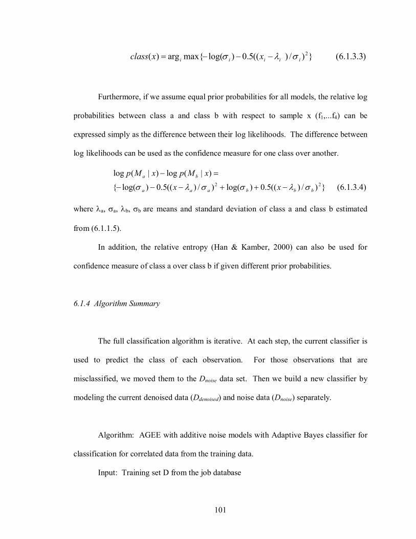
101

) 3 . 3 . 1 . 6 ( ) / ) (( 5 . 0 ) log( max arg ) ( 2 i i i i i x x class σ λ σ − − − =

Furthermore, if we assume equal prior probabilities for all models, the relative log

probabilities between class a and class b with respect to sample x (f1,...f4) can be

expressed simply as the difference between their log likelihoods. The difference between

log likelihoods can be used as the confidence measure for one class over another.

) 4 . 3 . 1 . 6 ( ) / ) (( 5 . 0 ) log( ) / ) (( 5 . 0 ) log(

) | ( log ) | ( log 2 2

b b b a a a

b a

x x x M p x M p

σ λ σ σ λ σ − + + − − −

= −

where λa, σa, λb, σb are means and standard deviation of class a and class b estimated

from (6.1.1.5).

In addition, the relative entropy (Han & Kamber, 2000) can also be used for

confidence measure of class a over class b if given different prior probabilities.

6.1.4 Algorithm Summary

The full classification algorithm is iterative. At each step, the current classifier is

used to predict the class of each observation. For those observations that are

misclassified, we moved them to the Dnoise data set. Then we build a new classifier by

modeling the current denoised data (Ddenoised) and noise data (Dnoise) separately.

Algorithm: AGEE with additive noise models with Adaptive Bayes classifier for

classification for correlated data from the training data.

Input: Training set D from the job database

102

Output: Classifier C for the job assignment process.

Method:

1. Ddenoised ← D, Dnoise ← ∅

2. Apply the GEE model on Ddenoised to obtain initial weight estimation

(w1,...,w4). Use the AIC criteria to decide which models are most appropriate i.e. add

interaction term or use different correlation structure.

3. Compute the mean, variance and conditional probability of each class

using (6.1.1.1) and (6.1.1.3). Proportion the mean and variance such that the estimation

from the AGEE model can be written as mixtural Gaussian model form:

) 1 . 4 . 1 . 6 ( ) , ( p 2i i

1 i σ λ φ ∑

=

= n

i y

where λi, σi and pi are mean, standard deviation and proportions of each class.

4. Model Dnoise as a mixture Gaussian distribution. Estimate the mixture

coefficients and parameters by Gibbs sampling with Bayesian framework. The prior

distribution uses Dirichlet function.

5. Use the modified Naive Bayes (NB) classifier to predict the class of each

observation x in Ddenoised. If an observation is misclassified, move it to Dnoise. The

classifier can be written as

) 2 . 4 . 1 . 6 ( ) | 1 ( ˆ ε + = = = y w decision P y

where ε is the model of the noise data.

6. Use AIC criterion and lowest misclassification rate to determine whether

the current classifier is satisfactory. If not, repeat step (2) – (5). The resulting model is

updated AGEE with an additive noise.

103

This model is used for further classifications and predictions.

6.1.5 AGEE with Gibbs Sampling under Bayesian Framework with AB Classifier

The similarity between AGEE with AB classifiers and SVM with RBF as model

and Adatron as learning algorithm is that both methods find out the confusion region,

which is the region where the model's generalization error rate is above a given threshold

(Boser, Guyon, & Vapnik, 1992; Cortes & Vapnik, 1995; Friess, Cristianini, &

Campbell, 1998),. The training processes focus on this region's data and using AGEE

models with AB classifier or SVM to gain the classification accuracy, which is based on

the idea of ensembling (Dietterich, 2000). The advantage of AGEE with AB classifiers is

that it can identify attributes of the data most useful for classification through GEE model

selection according to the Akaike Information Criteria (AIC). It also counts the

correlation structure among the outputs into the estimation of the mean and standard

deviation of each class (decision).

The Gibbs sampling with Bayesian framework can deal with noise and outliers

(which both come from the virtually non­deterministic, subjective nature of human

decision making) more efficiently and robustly through treating some output as missing

value and adding prior distribution to it. This can overcome drawbacks of the survey and

time delay effects on the output ‘decision’. Moreover it estimates the noise through

assessments of uncertainty in the posterior probabilities of belonging to classes. All these

important pieces of information are partially ignored in other classification methods,

104

which may make biased estimation and lower the reliability of the results. It also drops

the assumption of independence made by Naive Bayes algorithms (Han & Kamber,

2000). One assumption for our approach is that the distribution for each class of data

follows Gaussian distribution. From the Central Limit Theorem it can easily be shown

that it holds in most cases, especially for non­deterministic data. We will show that the

Gaussian distribution holds in our case using Skewness and Kurtosis statistics.

6.2 Experiment Results and Discussion

The weight estimations using AGEE with additive model are shown in table 6.1.

The four coefficients (Job Priority Match, Sailor Location Preference Match, Paygrade

Match, Geographic Location Match) can be obtained through normalization. Table 6.2

shows these values, which is now in a form that can be fed into IDA as coefficients. It

shows that job priority, paygrade and geographic location are far more important than

sailor location preference match. The best model for our case is without interaction and

using exchangeable correlation structure according to the AIC criterion. Table 6.3 gives

the estimated exchangeable correlation matrix.

105

Table 6.1. Parameter estimates (std: Standard Deviation, CI: 95% confidence interval)

with exchangeable working correlation matrix using AGEE with additive model

Parameter Estimate std 95% CI Z Pr >|Z| Intercept ­12.1456 1.0975 ­14.2967,

­9.9945 ­11.07 <.0001

Job priority 5.0002 0.9668 3.1053, 6.8951

5.17 <.0001

Location preference

0.5133 0.2466 0.0299, 0.9968

2.08 <0.0374

Paygrade 3.9618 0.3256 3.3236, 4.6000

12.17 <.0001

Geographic location

4.2431 0.5696 3.1266, 5.3595

7.45 <.0001

Table 6.2. Estimated coefficients with standard error for the soft constraints using FFNN

and AGEE with additive model (AS community)

Coefficient Policy Name Estimated Value with FFNN

Estimated value with AGEE

w1 (a1) Job Priority Match 0.316±0.048 0.365±0.071 w2 (a2) Sailor Location Preference Match 0.064±0.020 0.037±0.018 w3 (a3) Paygrade Match 0.358±0.029 0.289±0.024 w4 (a4) Geographic Location Match 0.262±0.046 0.309±0.042

Table 6.3. Exchangeable correlation matrix

Parameters Intercept Job priority Location preference

Paygrade Geographic location

Intercept 1.0000 ­0.7287 ­0.0958 ­0.5107 ­0.5940 Job priority ­0.7287 1.0000 0.0861 0.0568 0.0816 Location preference

­0.0958 0.0861 1.0000 0.0870 ­0.1805

Paygrade ­0.5107 0.0568 0.0870 1.0000 0.1333 Geographic location

­0.5940 0.0816 ­0.1805 0.1333 1.0000

106

Table 6.4 shows the mixture mean and standard deviation estimation of two

classes for denoised data from AGEE model. As it can be seen the statistics of Skewness

and Kurtosis of two classes are smaller than 3, so the Gaussian assumption for AB

classifier holds. Table 6.5 provides mean, standard deviation, median and Monte­Carlo

simulation error with 1000 iterations for noised data using Gibbs sampling with Bayesian

framework.

Table 6.4. Mixture Gaussian Distribution Estimation from denoised data using GEE with

Additive Model. (D: Decision, obs: observation)

D obs mean Std T Value Pr > |t| Skewness Kurtosis

0 1032 0.108368 0.154699 22.50 <.0001 1.764932 2.467487 1 161 0.513594 0.186938 34.86 <.0001 ­0.100617 1.185754

Table 6.5. The noise data estimation using Gibbs sampling under Bayesian framework

node mean std MC err. 2.5% median 97.5% start sample

P[1] 0.484 0.097 0.003 0.299 0.483 0.671 1 1000 P[2] 0.515 0.097 0.003 0.329 0.516 0.701 1 1000 λ[1] 0.754 0.038 0.001 0.675 0.756 0.821 1 1000 λ[2] 0.815 0.037 9.6E­4 0.742 0.814 0.897 1 1000 σ 0.141 0.023 8.9E­4 0.104 0.138 0.191 1 1000

The following figures show some simulation results of noise estimation using

BUGS software.

107

lambda[1] sample: 1000

0.2 0.4 0.6 0.8

0.0 5.0 10.0 15.0

P[1] sample: 1000

0.0 0.2 0.4 0.6

0.0 2.0 4.0

6.0

lambda[2] sample: 1000

0.7 0.8 0.9

0.0 5.0 10.0 15.0

P[2] sample: 1000

0.2 0.4 0.6 0.8

0.0 2.0 4.0

6.0

sigma sample: 1000

0.0 0.1 0.2 0.3

0.0 5.0 10.0 15.0 20.0

P[2]

iteration 1 250 500 750 1000

0.2

0.4

0.6

0.8

108

sigma

iteration 1 250 500 750 1000

0.0

0.1

0.2

0.3

0.4

lambda[2]

iteration 1 250 500 750 1000

0.6

0.7

0.8

0.9

6.3 Comparison of Methods

Table 6.6 compares different classification approaches with correct classification

rates. Nearest neighbor using normal density estimation, using Biweight density

estimation and Mahalanobis distances, data mining approaches like Multi­layer Percepton

(MLP) with back­propagation algorithms, Support Vector Machine (SVM) with Adatron

algorithms and Naive Bayes classifier are used. Comparison of NB with and without

(directly computing mean and standard deviation from data) GEE and Adaptive Bayes

classifiers combining with AGEE with additive models are also given in the same table.

The table shows that the Adaptive Bayes classifiers combined with AGEE with additive

models give much higher accuracy than three types of Nearest Neighbor (NN), and also

higher than the original Naive Bayes algorithms with or without using GEE with additive

model. The performance is very close to the best SVM with Adatron algorithm and MLP

109

with back­propagation and momentum algorithm with one hidden layer (15 hidden nodes,

best case). Note that AGEE model and algorithm complexity is less than that of SVM

and MLP, so the model­density based classifier is very efficient and robust to capture the

properties of "indeterministic" data and it makes human­like decisions.

Table 6.6. Correct classification rates for different approaches

Method Correct Classification Rate NN using normal kernel density 76.05% NN using Mahalanobis distances 77.52% NN using biweight kernel density estimation 81.65% NB without GEE 84.81% NB with GEE 85.75% AB with AGEE 93.42% MLP (15nodes, best case) 93.14% SVM 93.50%

To further improve the classification rates we applied our extra knowledge about

the data set. The surveyed detailer typically offered no more than one job to each sailor.

Offering only a job with the highest output value could greatly increase the classification

rate. Comparison before and after post­processing (using group ID) of the five

approaches discussed in this dissertation proposal is shown in Table 6.7. All the reported

values are based on 25% testing set. The table shows that the SVM gave the highest

classification accuracy, but it had relatively high time cost and standard deviation. The

performances of AB with GEE and MLP with 15 nodes are also encouraging. MLP also

had a very low time cost. The relatively high decision making capability of the ANFIS

gives us a reasonable way for future sampling of detailers, which doesn't depend on the

delicate noisy tuning of the functions for soft constraints, but its high time cost may make

110

it a poor choice for large data sets. Although the decision­making capability of the GLM

with logistic link function is the lowest among the reported methods, its low time and

architecture complexity may make it a good model candidate in case a large data set

becomes available in the future. Moreover this is the method, which mostly exploits the

exact definitions of the f1,...,f4 functions, so if we can somehow improve the definition of

these functions, this model may become a very useful tool for constraint satisfaction

purposes.

Some combination of the provided methods may also be useful to make up the

weaknesses of one another. For example, the structural learning with forgetting in MLP

generally has good approximation, robustness to noise and requires no preliminary

knowledge. However, it provides no explanation of the obtained results, which could be

done with fuzzy rules generated by the ANFIS.

Table 6.7. Average Running Times (RT) in seconds, average Correct Decision Making

Rates (CDMR) and average Correct Decision Making Rates after Post Processing (PP)

for different methods (average of 10 runs)

Method RT CDMR PP

GLM 170 87.4%±0.1% 91.2%±0.2% MLP 227 93.1%±0.1% 94.3%±0.2% ANFIS 3050 91.5%±0.4% 93.2%±0.3% SVM 1425 93.5%±1.0% 95.5%±0.6% AB 1035 93.4%±0.2% 95.2%±0.4%

Naturally, we can’t expect 100% correct classification rate because of the

presence of noise from various sources. (Note that in about 1% of the cases the surveyed

111

detailer offered 2 or more jobs to sailors, which couldn't be overcome with this

postprocessing method.) The most important perhaps is the indeterminate nature of

detailer decisions. Even the same detailer may easily make different decisions on the

same data at different times and different detailers are even more likely to make different

decisions even under the same circumstances. Moreover environmental changes further

bias decisions, so periodic training on up to date data sets is necessary in order to keep

constraint satisfaction up to date in IDA. As a result our reported and observed values

can't tell us how well our system makes decisions, but only how well it follows the

decisions given by the surveyed detailers. This problem is present in Navy practices as

well: they don't have a well­defined formula to effectively evaluate detailer performance.

6.4 Matching Multiple Sailors to Multiple Jobs

Matching multiple sailors to multiple jobs could have been a long­term objective

of IDA. However the classic n:m matching models (Gale & Shapley, 1962) can only be

applied with restrictions. Situations may change in a matter of minutes. New emails may

come, training classes may become filled by other detailers, and so on. Doing n:m

matching, including negotiations with sailors, could be time consuming, and by the end

of it some of the options may not be valid any more. However, a limited version of an

n:m matching applied to small groups of sailors in a narrow time frame could result in

better overall satisfaction of the stakeholders. Unfortunately this could mean that IDA

only offers one job instead of the desired two or three to each sailor, which would

probably not improve retention.

112

Any of the methods discussed in this dissertation can be expanded to n:m

matching, and are currently under investigation under a multi agent system framework.

Such optimization processes would look for a global fitness for a group of sailors in a

given time frame.

6.5 General Performance of AB with AGEE

6.5.1 Adaptive Generalized Estimation Equation for a Second Survey on the Aviation

Support Equipment Technician Community

As we have seen so far the AB with AGEE method is a new and innovative

method, which was designed to accommodate correlated data adaptively. Based on

experimental results discussed earlier in this chapter AB with AGEE provided higher

correct classification rates than other methods and gave accurate coefficients for IDA's

current constraint satisfaction module.

To verify the robustness and the efficiency of the AGEE method and to see how

reliable detailer decisions are we presented the same data to the same detailer at a

different time. As we have expected the detailer provided somewhat different decisions

for the second survey. Table 6.8 and table 6.9 provide the list of incorrect decisions

made by AGEE based on the first survey and the second survey, respectively. The

incorrect decisions made by the AGEE method on both surveyed data sets are marked

with *.

113

Table 6.8. The list of incorrect decisions made by AGEE based on the first survey after

post processing (offering only the highest output valued job over threshold for each

sailor). Those incorrect AGEE decisions, which were made on both surveys are marked

with *. obs = observation, id = group ID, P is probability of job to be offered (defined in

4.2.1.1), decisionfromP is the decision made by the model after post processing, decision

is the surveyed decision

obs id P decisionfromP decision 5 3 0.183339 1 0 6 3 0.096876 0 1 45 17 0.229877 1 0 58 22 0.07 0 1 * 62 23 0.017285 0 1 * 68 25 0.155264 1 0 73 25 0.000533 0 1 93 29 0.061519 0 1 95 30 0.159274 1 0 * 96 30 0.096876 0 1 *

124 35 0.359306 0 1 129 35 0.415732 1 0 155 38 0.134279 0 1 160 38 0.369966 1 0 173 39 0.417668 1 0 175 39 0.303144 0 1 228 47 0.082457 0 1 * 420 76 0.417668 0 1 * 506 80 0.415732 0 1 * 534 83 0.638168 1 0 * 536 83 0.442108 0 1 * 564 87 0.526338 1 0 * 567 87 0.415732 0 1 * 581 89 0.368111 0 1 * 827 109 0.415732 1 0 854 113 0.575776 1 0 * 857 113 0.228953 0 1 * 955 121 0.345254 0 1 * 962 122 0.056391 0 1 * 967 125 0.442173 1 0 * 977 131 0.4619 1 0 * 978 131 0.122215 0 1 * 996 140 0.417668 1 0 * 997 140 0.196389 0 1 *

1025 148 0.518236 0 1 obs id P decisionfromP decision 1039 150 0.391664 0 1 * 1044 151 0.391664 0 1 * 1059 153 0.391664 0 1 * 1149 167 0.021197 0 1 * 1150 168 0.015666 0 1 * 1151 169 0.019504 0 1 * 1153 170 0.015666 0 1 * 1154 171 0.026353 0 1 * 1156 172 0.026353 0 1 * 1159 173 0.225764 1 0 * 1219 187 0.028402 0 1 * 1221 189 0.028402 0 1 * 1222 190 0.028402 0 1 * 1223 191 0.028402 0 1 *

114

1224 192 0.028402 0 1 * 1225 193 0.028402 0 1 * 1332 223 0.056797 0 1 1342 227 0.235277 1 0 1346 227 0.075731 0 1 1407 231 0.089904 0 1 * 1447 234 0.705831 1 0 * 1448 234 0.415732 0 1 * 1533 250 0.036138 0 1 * 1537 252 0.197522 1 0 * 1558 253 0.156206 0 1 * 1587 255 0.185615 0 1 * 1596 255 0.520778 1 0 *

Table 6.9. The list of incorrect decisions made by AGEE based on the second survey

after post processing (offering only the highest output valued job over threshold for each

sailor). Those incorrect AGEE decisions, which were made on both surveys are marked

with *. obs = observation, id = group ID, P is probability of job to be offered (defined in

4.2.1.1), decisionfromP is the decision made by the model after post processing, decision

is the surveyed decision

obs id P decisionfromP decision 58 22 0.083616 0 1 * 62 23 0.021544 0 1 * 95 30 0.196581 1 0 * 96 30 0.105091 0 1 *

obs id P decisionfromP decision 228 47 0.10393 0 1 * 309 64 0.387864 1 0 310 64 0.093443 0 1 420 76 0.397307 0 1 * 506 80 0.387864 0 1 * 534 83 0.619117 1 0 * 536 83 0.440138 0 1 * 543 84 0.619117 1 0 545 84 0.440138 0 1 564 87 0.50445 1 0 * 567 87 0.387864 0 1 * 581 89 0.345721 0 1 * 622 92 0.332211 1 0 764 101 0.113066 0 1 810 107 0.441494 1 0 813 107 0.05284 0 1 854 113 0.549685 1 0 * 857 113 0.274761 0 1 * 955 121 0.344433 0 1 * 962 122 0.071951 0 1 * 967 125 0.419239 1 0 * 977 131 0.441593 1 0 * 978 131 0.151897 0 1 * 987 136 0.055751 0 1 996 140 0.397307 1 0 * 997 140 0.238449 0 1 *

1039 150 0.366537 0 1 * 1044 151 0.366537 0 1 *

115

1059 153 0.366537 0 1 * 1149 167 0.026735 0 1 * 1150 168 0.01971 0 1 * 1151 169 0.027763 0 1 * 1153 170 0.01971 0 1 * 1154 171 0.037547 0 1 * 1156 172 0.037547 0 1 * 1159 173 0.2255 1 0 * 1219 187 0.034814 0 1 * 1221 189 0.034814 0 1 * 1222 190 0.034814 0 1 * 1223 191 0.034814 0 1 * 1224 192 0.034814 0 1 * 1225 193 0.034814 0 1 * 1282 209 0.065253 0 1 1407 231 0.132596 0 1 * 1447 234 0.674147 1 0 * 1448 234 0.387864 0 1 * 1461 238 0.21704 1 0 1463 238 0.204013 0 1 obs id P decisionfromP decision 1466 239 0.21704 1 0 1468 239 0.204013 0 1 1469 239 0.020926 0 1 1471 240 0.21704 1 0 1473 240 0.204013 0 1 1476 241 0.241587 1 0 1533 250 0.035544 0 1 * 1537 252 0.232866 1 0 * 1558 253 0.18908 0 1 * 1587 255 0.225342 0 1 * 1596 255 0.510049 1 0 *

Table 6.8 and table 6.9 show that there were 45 incorrect decisions marked with

*. These decisions were the same (by the detailer) on both surveys and AGEE missed

them on both runs. This corresponds to about 3.5% of the data. We can also see in the

tables that additional 17 decisions were misclassified on the first and 18 on the second

surveyed data sets. These decisions truly lie on the fringe of correct decisions, where

even the same detailer made different decisions on the same data at different times.

Adding the above 17 to 18 we get 35, which divided by 1277 give about 2.7%, which is

the difference in the detailer decisions between the first and second surveys. This is far

lower than the estimated 20% difference, which was estimated by the same a detailer.

This low difference rate is partially due to the fact that the detailer was asked to make

decisions solely based on the four soft constraints.

116

On the other hand, the difference in decisions can also be defined based on groups

instead of individual decisions. In this case we find 22 decisions effecting groups id's

(sailors), which corresponds to about 8.6% difference. As a result 22 sailors would get

different offers from the detailer. Therefore this definition of "difference in decision" is

more meaningful and is closer to the detailer estimation.

Based on table 6.8 and table 6.9 we can see that the correct decision making rates

of AGEE are very close to each other, and are around 95.2% after post processing. Table

6.10 presents the coefficient estimations for the f1­f4 functions for the second data set

(corresponding to Table 6.9) for AGEE and the FFNN method.

Table 6.10. Estimated coefficients with standard error for the soft constraints using

FFNN and AGEE with additive model for the second data set (AS community)

Coefficient Policy Name Estimated Value with FFNN

Estimated value with AGEE

w1 (a1) Job Priority Match 0.313±0.047 0.363±0.075 w2 (a2) Sailor Location Preference Match 0.047±0.017 0.041±0.019 w3 (a3) Paygrade Match 0.321±0.026 0.268±0.022 w4 (a4) Geographic Location Match 0.319±0.050 0.328±0.044

The comparison of table 6.2 and table 6.10 provides a number of useful

information. First of all we can see that the change in coefficients did not exceed 0.057

on either methods, which means that learned coefficients based on a single survey are

meaningful and accurate for a single community. Also we can see that this change was

lower for the AGEE method than for the FFNN method, which means that AGEE results,

even based on a single survey are more robust than results of the FFNN. Lastly, we can

117

observe that the detailer considered Geographic Location Match to be more important for

the second survey than for the first survey.

The AGEE method not only proved to be more efficient for classification

problems with noisy, correlated output with grouped data but it can fit different scales of

data such as continuous data, ordinal data or categorical data as well. It also works well

for small sized data. More importantly the data may change dynamically, which can be

learned by the model adaptively, based on the accumulated history of the data including

the current data so decision can be made accordingly.

Because of the "No Free Lunch" theorem we know that there is no single method,

which works better for all problems than all the other methods. Since Adaptive

Generalized Estimation Equation with Bayes Classifier combines strengths of GEE with

Bayes classifier and some other techniques, it resolves the complex problems, and the

computational complexity is higher than other linear discriminant classification methods.

The best approach for analyzing any given data set is related to the type of the data, its

properties, the question being asked about that data and the goal to be achieved from that

data.

6.5.2 Adaptive Generalized Estimation Equation for the Aviation Machinist Community

To further test the AGEE method and to verify the robustness and the efficiency,

a different community, the Aviation Machinist (AD) community was chosen. 2390

"matches" for 562 sailors has passed preprocessing and the hard constraints. Before the

survey was actually done a minor heuristic tuning was performed to comfort the AD

118

community. The aim of such tuning was to make sure that the soft constraint functions

yield values on the [0,1] interval for the AD data. The data then was presented to an

expert AD detailer who was asked to offer jobs to the sailors considering only the same

four soft constraints as we have used before: Job Priority Match, Sailor Location

Preference Match, Paygrade Match, Geographic Location Match. The acquired data with

the surveyed Boolean decisions was sent through the AGEE classification method. For

comparison, FFNN was also applied to the same data. Table 6.11 provides the estimated

coefficients for the four soft constraints for the AD community using FFNN and AGEE

methods.

Table 6.11. Estimated coefficients with standard error for the soft constraints for the AD

community using FFNN and AGEE with additive model

Coefficient Policy Name Estimated Value with FFNN

Estimated value with AGEE

w1 (a1) Job Priority Match 0.010±0.002 0.010±0.002 w2 (a2) Sailor Location Preference Match 0.091±0.027 0.075±0.026 w3 (a3) Paygrade Match 0.786±0.075 0.760±0.082 w4 (a4) Geographic Location Match 0.113±0.041 0.155±0.047

As it can be seen in the table, the estimation of the two methods are very close to

one another for the AD data set and both show that the third function, Paygrade Match,

weigh more than the other three functions. This matches the fact that the detailer

considered one of the soft constraints, the Paygrade Match, much more important then

the other soft constraints. The corresponding correct classification rates were 94.6±0.1%

for the FFNN and 96.4%±0.1% for the AGEE after post processing. This demonstrates

that human like decisions were learned and made by the FFNN and the AGEE methods.

119

Post processing on this data was more important than on previous data: the

surveyed detailer offered exactly one job to each sailor more frequently than the other

detailer on previous surveys. Last, but not least, the AD detailer considered job priority

only as a tiebreaker: Job priority by itself never resulted in a denied decision. However,

if other soft constraints were equally satisfied then he always offered the job with the

highest job priority. Interestingly, this behavior was well captured by the AGEE model.

AGEE found that the coefficient for job priority was negative, but the corresponding P

value was over threshold. P value is used to accept or deny hypothesis. In this case it

meant that the old hypothesis: "the negative value can be accepted" was to be rejected,

and a new hypothesis had to be built. The coefficient for job priority had to be set to zero

or some positive value. We couldn't set it to zero, because the detailer admittedly

considered it, although only as a tiebreaker. We couldn't set it to a high positive value

because it would interfere with the other three values. However, a small positive value

(0.01) fit the model well and provided very good correct classification rate. Interestingly

FFNN also provided negative coefficient for f1, but it did not help to provide hypothesis

on its interpretation. However, after changing it to the same positive 0.01 FFNN also

provided good results.

6.5.3 Adaptive Generalized Estimation Equation for Microarray Data

To verify the efficiency and the boundary of our proposed AGEE with Bayes

Classifier method we applied the method to microarray gene expression data

experimented by Eisen et al (Eisen, Spellman, Brown, & Botstein, 1998). The extracted

120

data contains two classes: Ribosomal protein genes (121 samples) and non­ribosomal

protein genes (2346) with 79 various experimental conditions corresponding to 79

variables from the Stanford database. As expected the AGEE method did not provide

good results due to a number of reasons. One reason is that there were a large number of

attributes with high input interactions among them. The Maximum likelihood estimates

of AGEE do not exist and the convergence of the algorithm is questionable. Therefore

the validity of the model fit to this data is questionable. The error rate was high

compared to other well known methods, such as MLP. MLP with one hidden layer

provided 96.03% correct classification rate. This shows the weakness and the boundary

of the AGEE method. AGEE is not well suited to data with a large number of attributes

with high input interactions such as time series data. Please note that even this data could

be transformed into a form where AGEE would be more suitable by preprocessing, but it

would not surpass the performance of MLP. Such preprocessing should aim on the

reduction of the number of attributes, using feature selection or principle component

analysis.

6.6 Conclusion

The method discussed in this chapter can be extended to multi­class probability

estimation and classification problems. The approach can be used for any kind of

decision­making problem, like financial prediction problems, medical diagnoses, medical

prediction and so on. As it was mentioned earlier, the classifier had several additional

advantages compared to other classification methods. These include fewer assumptions,

121

less complexity of the model and algorithms, less likely to be trapped at local minimum,

can deal with data with high noise level and data with large number of attributes. The

computed density estimation could give a very good representation of the true

distribution due to the correlation structure of the output accounted for in the model and

also we model the noised data using Gibbs sampling with Bayesian framework, so it is

more efficient and it can posses good generalization performance. The obtained

classification result is close to that of the Support Vector Machine's and with somewhat

lower time complexity and lower standard deviation. Due to all these advantages AGEE

may be the most efficient tool to handle constraint satisfaction in IDA, in spite of its

deep statistical properties, not offering cognitive properties. However, some people may

argue that the brains are little more than massive statistical tools collecting and

processing data and providing predictions largely untraceable for outside observers.

AGEE besides classification also provides coefficients usable in IDA's current linear

functional approach for constraint satisfaction. These coefficients are more accurate than

those provided by FFNNs through logistic regression.

In the next chapter we summerize all the work done in this dissertation and

provide some possible future directions of work concerning IDA, constraint satisfaction

and decision making.

122

7 Conclusion

7.1 What Has Been Done

Some of the contributions already achieved by this work include a design and

implementation of a working constraint satisfaction module within the intelligent agent

framework, which is able to support decision making efficiently. Such efficiency was

acquired through design, implementation and testing of a wide variety of machine

learning approaches, careful surveys of Navy experts and study of the vast data provided

by the Navy. Among others an innovative ensembling approach for prediction was

invented, designed, implemented and tested, which combines advanced statistical

learning and data mining techniques. Design and implementation of a "conscious"

constraint satisfaction has also been completed, which cognitively models humans within

the cognitive agent architecture. Constraint satisfaction was also designed and

implemented such a way that it fit's the "behavior network" action selection concept.

Contribution to the research in intelligent agents and machine learning has also been

demonstrated with publications.

Thorough testing of the new ensembling method (AGEE) and the FFNN have

been completed, which were based on three separate Navy surveys on two communities

and some randomly chosen unrelated data set. Such tests provided more reliable and

precise results, such as classification rates, coefficients for IDA’s constraint satisfaction

module, standard deviations, running times and so on. It has been seen that results of

AGEE are good and robust for data with high noise, output correlation and low number

123

of attributes, such as the available Navy data. However, it did not work well for data

with high input correlation and high number of attributes. FFNN and AGEE are

methods, which provided effective coefficients for IDA’s constraint satisfaction module.

ANFIS has helped us to build hypothesis on how human detailers make decisions for

constraint satisfaction problems. Comparison of the discussed methods has been

provided, which focused on the needs of IDA, complexity issues, applicability and

cognitive issues. Discussion of how closely the discussed methods are coupled to the

data and the given problem helped to predict model suitability to other problems. Finally,

the design and implementation issues of IDA’s constraint satisfaction module have been

taken over to IDA's successor, the Multi Agent Naval Resource Distribution (MANRD)

in the form of sailor, Navy and command constraint satisfaction modules.

7.2 What Has Been Learned

In this dissertation IDA, an Intelligent Distribution Agent to automate the job

assignment problem of the US Navy, was described with the main concern being its

constraint satisfaction module. High­quality decision making using optimum constraint

satisfaction is an important goal of IDA, to aid the Navy to achieve the best possible

sailor, command and Navy satisfaction performance. A number of neural networks and

statistical approaches were created, applied, and tested to either improve the performance

of the current way IDA handles constraint satisfaction or to come up with alternatives to

the current linear functional approach. IDA's constraint satisfaction module, neural

networks and advanced statistical methods are complementary with one another. It has

124

been learned that to achieve a good general model of human behavior and decision

making in an artificial intelligent system constraint satisfaction, machine learning, and

statistical assessment have to be assembled automatically within the intelligent system.

We have also learned that intelligent behavior and decision making in an intelligent

system can be boosted through adaptation to environmental changes and the right data

has to be provided (or acquired by the system) to be used as training data in sufficient

quantity and frequency. Having learned all these about artificial intelligent systems we

can build a theory that automatic integration of constraint satisfaction, learning, and

statistical assessment is necessary for the emergence of human (or any) intelligence.

Moreover high level human (or any) intelligence requires adaptation to environmental

changes and efficient training data has to be provided (or the intelligent system can

collect it itself) in sufficient quantity and frequency to the system. We have also learned

that "conscious" software agents can be used to automate human information tasks,

where even constraint satisfaction needs to be "conscious" to help the agent to deal with

truly novel situations. However it is also learned that routine situations with novel

content don't require "consciousness" in constraint satisfaction. It has also been learned

that cognitive modeling can model large areas of cognition, which may occasionally lead

to emerging theories of human cognition. Moreover it has been learned that building

software based on cognitive modeling often demands vast computational power from

today's computers and many tasks can be performed more efficiently without cognitive

modeling ("airplanes don't flap their wings").

Results so far show that the Support Vector Machine is capable of making the

highest quality of human like decisions, although with high standard deviation and time

125

cost. Other methods also performed well, and they can be reasonable choices for future

needs in IDA, each offering some advantage, such as running time, robustness, and

model complexity, over the others. The Adaptive Generalized Estimation Equation with

Bayes Classifier provided nearly as good classification as the Support Vector Machine

but with a lower time complexity and standard deviation. Coefficients for the soft

constraints were also learned with this model. Due to this fact FFNNs and the AGEE can

be used as external modules from IDA, sparing the agent's architecture from growing

more complex, while preserving the current constraint satisfaction module. Feed

Forward Neural Network with logistic regression has learned coefficients well enough

with a very low time and model complexity. Multi Layer Perceptron with FFNN

provided the lowest standard deviation of all the discussed methods. Neural networks,

may also offer a better model of human cognition than the current linear functional

approach for constraint satisfaction. An Adaptive Neuro­Fuzzy Inference System can

even create and learn rules, which is similar to human knowledge discovery to support

decision making and partially make up the notorious "black box" nature of neural

networks. Moreover ANFIS is the most suitable to the Navy provided data, because it

doesn't depend deeply on the exact values of the soft constraint functions and enables

surveys in terms of linguistic descriptions. Analysis of the ANFIS also provided a

hypothesis on how human detailers and humans in general do constraint satisfaction for

decision making problems with the help of rules. It has also been learned that those rules

are in fact fuzzy even for human constraint satisfaction.

Based on knowledge of internal correlation of the data, postprocessing was

applied, which further improved constraint satisfaction performance for all presented

126

methods. Due to the noise, the uncertainty, and the rapidly changing environment of the

Navy's job assignment problem it is clear that a final optimum setup of the coefficients in

the linear functional or a model which doesn't need additional training don't exist, so

periodic tuning of any decision making mechanism is necessary. No matter which model

we choose to place online as part of a possible IDA product, data needs to be provided to

the agent periodically in order to allow up to date decision­making through learning.

7.3 How to Integrate the Discussed Modules into IDA

The discussed neural network and statistical modules are currently used off line

from IDA. Integration is possible but performance after integration is predictable. We

have already seen how FFNN and AGEE can be used to find numeric coefficients for

IDA’s constraint satisfaction module. Results obtained from AGEE are currently used in

IDA, which provides the best correct classification rate. These modules could be used as

external modules, where IDA would periodically submit the data to the module, say the

AGEE, which would perform training and would provide updated coefficients to IDA.

Code of IDA then would be updated with one of the methods discussed in chapter 3.

Any of the discussed methods could be integrated with IDA as an internal

module. Any neural network method can replace IDA’s current constraint satisfaction

module, because they produce an output value in the output layer, which is normalized

into [0,1]. These values are used to provide classification, where higher values

correspond to "offer" decisions and therefore they can be thought of as fitness values.

Most of IDA’s other modules would not change anything, because they would only feed

127

on the fitness values, not the architecture of a constraint satisfaction module. However

the overall architecture and time complexity would significantly increase and as we have

seen the performance of the AGEE method would not be surpassed anyway. Pure

statistical methods, such as AGEE can also be made part of IDA, and because of they can

provide coefficients, fitness values can be earned as well. Yet, making such modules run

through for every IDA cycle would be a major waste of time without any benefit.

Therefore we conclude that the optimal way IDA’s constraint satisfaction should be done

is with the current linear functional constraint satisfaction module, where functions are

updated periodically and heuristically based on domain specific knowledge. Coefficients

should be learned by AGEE periodically and fed into IDA’s constraint satisfaction

module, just like the way it has been discussed in this dissertation.

A question remains is whether consciousness can be and should be used for any of

the alternative modules if they are integrated with IDA. A fitness value produced by any

method can be made conscious and it would be treated exactly the same way as it has

been discussed in this dissertation. It would not affect IDA in any way differently than

discussed except the numerical values of the fitness. If we chose to make only the

decisions (offer or deny) conscious that would weaken IDA. Activations obtained at

neurons on other than the output layer can also be made conscious but it would not

provide any improvement in IDA and we don’t believe that such thing could or should

happen in humans or other intelligent agents. Although structural learning can be a

source of intelligence it only changes the constraint satisfaction module; all other

modules stay the same. Therefore the change in intelligence can be measured with the

change in quality decisions in the constraint satisfaction module. Changing rules in

128

ANFIS would result in different fitness values, which would provide different decisions

in IDA. Again, change in intelligence can be measured in the change in decisions in the

constraint satisfaction module.

129

References

Agrawal, R., Mannila, H., Srikant, R., Toivonen H. and Verkamo, A. (1996). Fast

Discovery of Associstion Rules. In Advances in Knowledge Discovery and Data

Mining, MIT Press, pp. 307­328.

Akaike, H. (1974). A new look at the statistical model identification. IEEE Trans.

Automatic Control, Vol. 19, No. 6, pp. 716­723.

Albert I., Jais, J. P. (1998). Gibbs Sampler for the Logistic Model In the Analysis of

Longitudinal Binary Data. Statist. Med.17, 2905­2921.

Ali, A. I., Kennington, J. L. and Liang, T. T. (1993). Assignment with En Route Training

of Navy personnel. Naval Research Logistics, Vol 40, pp. 581­592.

Anlauf J. K. and Biehl, M. (1989). The Adatron: an adaptive perceptron algorithm.

Europhysics Letters, 10(7), pp. 687­­692.

Baars, B. J. (1988). A Cognitive Theory of Consciousness. Cambridge University Press,

Cambridge.

Baars, B. J. (1997). In the Theater of Consciousness. Oxford University Press, Oxford.

Bayardo R. and Agrawal, R. (1999). Mining the most interesting rules. In ACM KDD

Conference.

Biganzoli, E., Boracchi, P., Mariani, L. and Marubini, E. (1998). Feed Forward Neural

Networks for the Analysis of Censored Survival Data: A Partial Logistic

Regression Approach. Statistics in Medicine, 17, pp. 1169­1186.

Bishop, C. M. (1995). Neural Networks for Pattern Recognition. Oxford University

Press.

130

Bogner, M. (1999). Realizing "consciousness" in software agents. Ph.D. Dissertation,

The University of Memphis, Memphis, TN, USA.

Bogner, M., Ramamurthy, U. and Franklin, S. (2000). “Consciousness" & Conceptual

Learning in a Socially Situated Agent. In Human Cognition and Social Agent

Technology, ed. K. Dautenhahn. Amsterdam: John Benjamins. 113­135

Boser, B., Guyon, I. and Vapnik, V. (1992). A Training Algorithm for Optimal Margin

Classifiers. In Proceedings of the Fifth Workshop on Computational Learning

Theory, pp. 144­152.

Cortes C. and Vapnik, V. (1995). Support vector machines, Machine Learning, 20, pp.

273­297.

Cristianini N. and Shawe­Taylor, J. (2000). An Introduction to Support Vector Machines

(and other kernel­based learning methods). Cambridge University Press.

Cun, Y. L., Denker, J. S. and Solla, S. A. (1990). Optimal brain damage. In D. S.

Toureczky, ed. Adavnces in Neural Information Processing Systems 2 (Morgan

Kaufmann), pp. 598­606, 1990.

Dietterich, T. G. (2000). Ensemble methods in machine learning. In Multiple Classier

Systems, First International Workshop, MCS 2000, Cagliari, Italy, pages 1­15.

Springer­Verlag.

Eisen, M. B., Spellman, P. T., Brown, P. O. and Botstein, D. (1998). Cluster analysis and

display of genome­wide expression patterns. PNAS, Vol. 95, Issue 25, 14863­

14868.

Fraley, C., Raftery, A. E. (2000). Model­Based Clustering, Discriminant Analysis, and

Density Estimation. Technical Report NO.380, 2000.

131

Franklin, S. (1995). Artificial Minds. Cambridge, Mass.: MIT Press.

Franklin, S. and Graesser, A. (1997). Is it an Agent, or just a Program?: A Taxonomy for

Autonomous Agents. Intelligent Agents III, Berlin: Springer Verlag, 21­35.

Franklin, S., Kelemen, A. and McCauley, L. (1998). IDA: A Cognitive Agent

Architecture. In the proceedings of IEEE International Conference on Systems,

Man, and Cybernetics ’98, IEEE Press, pp. 2646­2651.

Franklin, S. (2000). Deliberation and Voluntary Action in ‘Conscious’ Software Agents.

Neural Network World 10:505­521.

Franklin, S. (2001). Automating Human Information Agents. In Practical Applications of

Intelligent Agents, ed. Z. Chen, and L. C. Jain. Berlin: Springer­Verlag.

Friedman, J., Hastie, T. and Tibshirani, R. (2000). Additive Logistic Regression: a

Statistical View of Boosting. Technical Report.

Friess, T. T., Cristianini N. and Campbell, C. (1998). The kernel adatron algorithm: a fast

and simple learning procedure for support vector machine. In Proc. 15th

International Conference on Machine Learning, Morgan Kaufman Publishers.

Gale, D. and Shapley, L. S. (1962). College Admissions and stability of marriage. The

American Mathematical monthly, Vol 60, No 1, pp 9­15.

Gelfand, A. E., Hills, S. E., Racine­Poon A. and Smith, A. F. M. (1990). Illustration of

Bayesian inference in normal data models using Gibbs sampling. Journal of the

American Statistical Association, 85 (412), pp. 972–985.

Girosi, F., Jones M. and Poggio, T. (1995). Regularization theory and neural networks

architectures. Neural Computation, 7:219­­269.

132

Han, J. and Kamber, M. (2000). Data Mining Concepts and Techniques. Morgan

Kaufmann Publishers.

Haykin, S. (1999). Neural Networks. Prentice Hall Upper Saddle River, New Jersey.

Hofstadter, D. and Mitchell, M. (1994). The copycat project: A model of mental fluidity

and analogy­making. In Holyoak, K. and Barnden, J., editors, Advances In

Connectionist And Neural Computation Theory, volume 2: Analogical

Connections, Norwood, NJ. Ablex.

Horton, N. J. and Lipsitz, S. R. (1999). Review of Software to Fit Generalized Estimation

Equation Regression Models. The American Statistician, Vol.53.

Ishikawa, M. (1996). Structural learning with forgetting. Neural Networks, Vol. 9, pp.

509­521.

James, W. (1890). The Principles of Psychology. Harvard University Press, Cambridge,

MA.

Kanerva, P. (1988). Sparse Distributed Memory. Cambridge, Mass.: MIT Press.

Keller, A. D., Schummer, M., Hood L. and Ruzzo, W. L. (2000) Bayesian Classification

of DNA Array Expression Data. Technical Report UW­CSE­2000­08­01.

Kondadadi, R. (2001). Deliberative decision making in software agents. Master's Thesis,

The University of Memphis.

Kondadadi, R., Dasgupta, D. and Franklin, S. (2000). An Evolutionary Approach For Job

Assignment. Proceedings of International Conference on Intelligent Systems­

2000, Louisville, Kentucky, pp.139­142.

133

Kondadadi, R. and Franklin, S. (2001). A framework of deliberative decision making in

“conscious” software agents. To appear in the proceedings of International

Symposium on Artificial Life and Robotics–2001, Japan.

Kozma, R., Harter, D. and Achunala, S. (2002). Action Selection Under Constraints:

Dynamic Optimization of Behavior in Machines and Humans. Proceedings of the

IEEE International Joint Conference on Neural Networks, 2002, Hawaii, pp.

2574­2580.

Kozma, R., Sakuma, M., Yokoyama, Y. and Kitamura, M. (1996). On the Accuracy of

Mapping by Neural Networks Trained by Backporpagation with Forgetting.

Neurocomputing, Vol. 13, No. 2­4, pp. 295­311.

Liang K. Y. and Zeger, S. L. (1986). Longitudinal Data Analysis Using Generalized

Linear Models. Biometrika, 73, pp. 13­22.

Liang, T. T. and Thompson, T. J. (1987). Applications and Implementation – A large­

scale personnel assignment model for the Navy. The Journal For The Decisions

Sciences Institute, Volume 18, No. 2 Spring.

Liang, T. T., Buclatin, B. B. (1988). Improving the utilization of training resources

through optimal personnel assignment in the U.S. Navy. European Journal of

Operational Research 33 183­190 North­Holland.

Maes, P. (1990). How to do the right thing. Connection Science 1(3), pp.291–323.

Maes, P. (1992). Learning Behavior Networks from Experience. In F. J. Varela and P

Bourgine (Eds.), Toward a Practice of Autonomous Systems, Proceedings of the

First European Conference on Artificial Life. MIT Press/Bradford Books.

134

McCauley, L. (1999). Implementing Emotions in Autonomous Agents. Master Thesis,

The University of Memphis.

McCauley, L., Franklin, S., and Bogner, M. (1999). An Emotion­Based "Conscious"

Software Agent Architecture, Proceedings of the International Workshop on

Affect in Interactions Towards a New Generation of Interfaces, Siena, Italy. New

York: Springer­Verlag.

McLachlan, G., Peel, D. (2000). Finite Mixture Models. John Wiley & Sons, Inc.

Miller D. A. and Zurada, J. M. (1998). A dynamical system perspective of structural

learning with forgetting. IEEE Transactions on Neural Networks, vol. 9, no. 3, pp.

508­515.

Minsky, M.L. (1987). The Society of Mind, Cambridge. MA: MIT Press.

Mitchell, M. and Hofstadter, (1991). D. R. The Emergence of Understanding in a

Computer Model of Concepts and Analogy­making. Physica D 42: 322­34.

Reprinted in S. Forrest, ed., Emergent Computation. Cambridge, Mass.: MIT

Press.

Mitchell, M. (1993). Analogy­Making as Perception. Cambridge, Mass.: MIT Press,

1993.

Muller, K.­R., Mika, S., Ratsch, G. and Tsuda, K. (2001). An introduction to kernel­

based learning algorithms. IEEE Transactions on Neural Networks, 12(2):181­

201.

Negatu, A., Franklin, S. (2002). An Action Selection Mechanism for 'Conscious'

Software Agents. Journal of Cognitive Science Quarterly, special issue on

"Desires, Goals, Intentions, and Values: Computational Architectures" (in press).

135

Ramamurthy, U. Bogner, M. and Franklin, S. (1998). Conscious Learning In An

Adaptive Software Agent. In Proceedings of The Second Asia Pacific Conference

on Simulated Evolution and Learning, pp.24­27, Canberra, Australia.

Rissanen, J. (1978). Modeling by shortest data description. Automat., Vol. 14, pp. 465­

471.

Scholkopf, B., Sung, K., Burges, C., Girosi, F., Niyogi, P., Poggio, T. and V. Vapnik

(1997). Comparing support vector machines with gaussian kernels to radial basis

function classifiers. IEEE Trans. Sign. Processing, 45:2758 ­­ 2765, AI Memo

No. 1599, MIT, Cambridge.

Schumacher, M., Rossner R. and Vach, W. (1996). Neural networks and logistic

regression: Part I'. Computational Statistics and Data Analysis, 21, pp. 661­682.

Spiegelman, D., Rosner B. and Logan, R. (2000). Estimation and Inference for logistic

Regression with Covariate Misclassification and Measurement Error in main

Study/Validation Study Designs. Journal of the American Statistical Association,

95(449): pp. 51–61.

Song, H. and Franklin, S. (2000). A Behavior Instantiation Agent Architecture.

Connection Science, Vol. 12, pp.21­44.

Stone, M. (1974). Cross­validatory choice and assessment of statistical predictions (with

discussion). Journal of the Royal Statistical Society, Series B, 36, pp. 111­147.

Tsoukalas L. H. and R. E. Uhirg, (1997). Fuzzy and Neural Approaches in Engineering.

John Wiley & Sons, N. Y.

Appendix

137

Author's Related Publications

Kelemen, A., Liang, Y., Kozma, R., and Franklin, S., "Optimizing Intelligent Agent's

Constraint Satisfaction with Neural Networks", in: "Innovations in Intelligent

Systems" (A. Abraham, B. Nath, Eds.), in the Series "Studies in Fuzziness and

Soft Computing", Springer­Verlag, Heidelberg, Germany, 2002 (in press).

Kelemen, A., Liang, Y., and Franklin, S., "A Comparative Study of Different Machine

Learning Approaches for Decision Making", in: "Recent Advances in Simulation,

Computational Methods and Soft Computing" (N. E. Mastorakis, ed.) in the

"Electrical and Computer Engineering Series", WSEAS Press, Piraeus, Greece,

pp. 181­186, 2002.

Kelemen, A., Kozma, R., and Liang, Y., "Neuro­Fuzzy Classification for the Job

Assignment Problem", in the proceedings of the IEEE International Joint

Conference on Neural Networks, Hawaii, pp. 1831­1837, 2002.

Kelemen, A., Liang, Y., Kozma, R., Franklin, S., and George, E. O., "Optimizing

Decision Making with Neural Network in Software Agents", IEEE Transactions

on System, Man and Cybernetics, 2002 (in review).

Kelemen, A., and Franklin, S., "The Constraint Satisfaction Module in IDA", Journal of

Applied Artificial Intelligence, 2002 (in review).

Liang, Y., Lin, K., and Kelemen, A., "Adaptive Generalized Estimation Equation with

Bayes Classifier for the Job Assignment Problem", in: "Advances in Knowledge

Discovery and Data Mining" (M. Chen, P. S. Yu, B. Liu, Eds.) in the "Lecture

138

Notes In Artificial Intelligence Series", Springer­Verlag, Heidelberg, Germany,

pp. 438­450, 2002.

Franklin, S., Kelemen, A., and McCauley, L., "IDA: A Cognitive Agent Architecture", in

IEEE Conference on Systems. Man and Cybernetics, IEEE Press, 2646­2651,

1998.