Constraint Qualiﬁcations and Stationarity Concepts for ... · 3.2.3 Comparison between the basic CQ ... convS convex hull of the set S cl(S) ... x ≥ y componentwise comparison

Constraint Qualifications and Stationarity

Concepts for Mathematical Programs with

Equilibrium Constraints

Michael L. Flegel

DissertationInstitute of Applied Mathematics and Statistics

University of Wurzburg

Constraint Qualifications and Stationarity

Concepts for Mathematical Programs with

Equilibrium Constraints

Dissertation zur Erlangung desnaturwissenschaftlichen Doktorgrades

der Bayerischen Julius-Maximilians-Universitat Wurzburg

vorgelegt von

Michael L. Flegel

aus

Bad Kreuznach

Wurzburg, 2005

Eingereicht am: 9. Dezember 2004bei der Fakultat fur Mathematik und Informatik

1. Gutachter: Prof. Dr. Christian Kanzow, Universitat Wurzburg2. Gutachter: Prof. Dr. Jirı Outrata, Czech Academy of Sciences

Tag der mundlichen Prufung: 11. Marz 2005

To my parents.

øXñK. àYJÓP@ øAg. é» A» ø@

øXñK. àYJP @P PðX èP áK@ AK¸A g ÈX P@ ÈA P@ Që Y ùK P@ A»

øXñK. àYJÓX QK. YJÓ@ áÒk YJ K AÓÐAJ k QÒ« HAJ«AK. P —

“Would but the Desert of Fountain yieldone glimpse—if dimly, yet indeed, reveal’d,Toward which the fainting Traveler might spring,As springs the trampled herbage of the field!”

— Omar Khayyam, The Rubaiyat

Preface

The doctoral thesis you hold in your hands is the result of research conducted during mytime as a post-graduate student at the Institute for Applied Mathematics and Statisticsat the University of Wurzburg. Its creation was a gradual process, intermediate goalsmanifesting in various preprints and papers. These can be seen as snapshots in time ofthe evolution of the material, the field, and myself that lead to the results found in thefollowing pages.

It was in large part the insights and ideas of my supervisor, Christian Kanzow, that leadto the creation of our publications, and thereby inevitably to the creation of this thesis.At several points during its inception, it could have swayed onto a different path than wasultimately followed. The reason for its current form may be found in the guidance and, attimes, purposeful restraint thereof, by Christian Kanzow. I am greatly indebted to him,not only professionally, but also personally, for providing me with this opportunity and foralways being there when I needed his help. He has my deepest gratitude.

It was also him that introduced me to the international community of researchers in myfield. Of these, I am particularly grateful to Jirı Outrata for agreeing to be the co-refereeof this thesis, and also for the many interesting discussions on MPECs and more generaltopics that lead to some joint work with him and Christian Kanzow. Also, he pointed outan error in an early draft of Section 5.3, suggesting a fix, which I gratefully incorporatedin the form of Lemma 5.26.

Another researcher who was of great help is Jane Ye. I thank her, in particular, for thein-depth discussions we had about the material covered in Section 5.2. Though I wouldlike to take credit for it, this material is solely due to her.

As much as the content of this thesis is based on rigorous mathematical reasoning, itwould not have been possible without the support I had at home, from my parents, mybrother Sven, Oma, and my greater family. It was them that helped me through frustratingand trying times, as well as being there to share in the joyous moments. Thank you.

This thesis went through several drafts before reaching its current form. My thanksgo out to Christian Nagel for proof-reading parts of the draft. Also, once more, ChristianKanzow proof-read large parts if not all of the material reproduced here (and in some casespenning them himself), simply due to his involvement in the publications that lead up tothis thesis.

A few other people deserve special mention: Alexis Iglauer, for being a good friend; mycolleagues (too many to all be listed; you know who you are), for providing a pleasant work-

viii Preface

ing environment; Carl Geiger, for igniting my love for mathematics; Manfred Dobrowolski,for his help in creating Figure 2.1; my students, for giving me something to look forwardto every week; and finally, Niloufar Hoevels, for her help in selecting the quotation foundon the previous page.

Michael L. Flegel Wurzburg, March 2005

Contents

1 Introduction 1

I Constraint Qualifications 7

2 Standard Constraint Qualifications 92.1 The Standard Nonlinear Program . . . . . . . . . . . . . . . . . . . . . . . 9

2.1.1 The Tangent and Linearized Tangent Cone . . . . . . . . . . . . . . 122.2 Application to MPECs . . . . . . . . . . . . . . . . . . . . . . . . . . . . . 17

2.2.1 The Abadie Constraint Qualification . . . . . . . . . . . . . . . . . 182.2.2 The Guignard Constraint Qualification . . . . . . . . . . . . . . . . 22

3 MPEC Constraint Qualifications 273.1 The Tightened Nonlinear Program . . . . . . . . . . . . . . . . . . . . . . 27

3.1.1 Relationship to Standard CQs . . . . . . . . . . . . . . . . . . . . . 293.2 The MPEC-Linearized Tangent Cone . . . . . . . . . . . . . . . . . . . . . 32

3.2.1 Sufficient Conditions for MPEC-ACQ . . . . . . . . . . . . . . . . . 353.2.2 Specific MPECs . . . . . . . . . . . . . . . . . . . . . . . . . . . . . 373.2.3 Comparison between the basic CQ [42] and MPEC-ACQ . . . . . . 43

3.3 Revisiting the Guignard CQ . . . . . . . . . . . . . . . . . . . . . . . . . . 46

II Stationarity Concepts 51

4 Necessary Optimality Conditions for MPECs 534.1 A Standard Nonlinear Programming Approach . . . . . . . . . . . . . . . . 534.2 A Direct Application to MPECs . . . . . . . . . . . . . . . . . . . . . . . . 554.3 An Indirect Application to MPECs . . . . . . . . . . . . . . . . . . . . . . 604.4 First Order Optimality Conditions under MPEC-GCQ . . . . . . . . . . . 68

5 M-Stationarity 715.1 Preliminaries . . . . . . . . . . . . . . . . . . . . . . . . . . . . . . . . . . 715.2 An Exact Penalization Approach . . . . . . . . . . . . . . . . . . . . . . . 805.3 A Direct Proof . . . . . . . . . . . . . . . . . . . . . . . . . . . . . . . . . 91

x Contents

III

6 Numerical Experiments 976.1 Overview . . . . . . . . . . . . . . . . . . . . . . . . . . . . . . . . . . . . . 976.2 Exact Penalization . . . . . . . . . . . . . . . . . . . . . . . . . . . . . . . 1006.3 A Bundle Trust Region Implementation . . . . . . . . . . . . . . . . . . . . 105

6.3.1 Application to the MacMPEC Test Suite . . . . . . . . . . . . . . . 112

Final Remarks 121

Bibliography 123

Abbreviations xi

Abbreviations

ACQ Abadie constraint qualificationAMPL a mathematical programming languageBT bundle trust regionCQ constraint qualificationGCQ Guignard constraint qualificationLICQ linear independence constraint qualificationMFCQ Mangasarian-Fromovitz constraint qualificationMPAEC mathematical program with affine equilibrium constraintsMPCC mathematical program with complementarity constraintsMPEC mathematical program with equilibrium constraintsNCP nonlinear complementarity problemNLP nonlinear programOPVIC optimization problem with variational inequality constraintsSCQ Slater constraint qualificationSMFCQ strict Mangasarian-Fromovitz constraint qualificationSQP sequential quadratic programmingTNLP tightened nonlinear programWSCQ weak Slater constraint qualification

xii Notation

Notation

Spaces and Orthants

R the real numbersR− the left half lineR+ the right half lineRn the n-dimensional real vector spaceRn− the nonpositive orthant in Rn

Rn+ the nonnegative orthant in Rn

Sets

x the set consisting of the vector xconvS convex hull of the set Scl(S) closure of the set SS1 ⊆ S2 S1 is a subset of S2

S1 ⊂ S2 S1 is a proper subset of S2

S1\S2 the set of elements contained in S1 but not in S2

Bε(z) open ball of radius ε around z(a, b) an open interval in R[a, b] a closed interval in R|δ| cardinality of the set δα i | Gi(z

∗) = 0, Hi(z∗) > 0

β i | Gi(z∗) = 0, Hi(z

∗) = 0, degenerate or biactive setγ i | Gi(z

∗) > 0, Hi(z∗) = 0

P(β) set of partitions of βZ the feasible region of the MPEC

Vectors

x ∈ Rn column vector in Rn

(x, y) column vector (xT , yT )T

xi i-th component of xxδ vector in R|δ| consisting of components xi, i ∈ δx ≥ y componentwise comparison xi ≥ yi, i = 1, . . . , nx > y strict componentwise comparison xi > yi, i = 1, . . . , nminx, y the vector whose i-th component is minxi, yimaxx, y the vector whose i-th component is maxxi, yi‖x‖ Euclidean norm of x‖x‖q q-norm of x

ei ∈ Rn the i-th vector of the canonical basis of Rn

Notation xiii

Cones

T (z∗) tangent cone to the feasible set Z of the MPEC at z∗

T (z∗,D) tangent cone to an arbitrary set D at z∗

T lin(z∗) linearized tangent cone of the MPEC at z∗

T linMPEC(z∗) MPEC-linearized tangent cone of the MPEC at z∗

N(v, Ω) Frechet normal cone to Ω at vNπ(v, Ω) proximal normal cone to Ω at vN(v, Ω) limiting normal cone to Ω at vNCl(v, Ω) Clarke normal cone to Ω at vN conv(v, Ω) convex normal cone to convex Ω at vC∗ dual cone of C

Functions

f : Rn → Rm function that maps Rn to Rm

fi : Rn → R i-th component function of fgph f graph of the function fepi f epigraph of the function fΦ : Rp ⇒ Rq a multifunction that maps Rp to subsets of Rq

gph Φ graph of the multifunction Φ∇f(z) gradient of the function f : Rn → R at z, column vector∇xf(x, y) gradient of f with respect to the variable xf ′(z) Jacobian in Rm×n of f : Rn → Rm at z

∂f(z) Frechet subgradient of a function f : Rn → R∂πf(z) proximal subgradient of a function f : Rn → R∂f(z) limiting subgradient of a function f : Rn → R∂Clf(z) Clarke subgradient of a function f : Rn → R∂convf(z) convex subgradient of a convex function f : Rn → RΠX(x) a (not necessarily unique) projection of x onto a closed set Xdist(x,X) Euclidean distance between x and closed XPq(·; ρ) exact lq MPEC-penalty function

Sequences

ak ⊆ Rn a sequence in Rn

ak → a a convergent sequence with limit aak a a convergent sequence in R with limit a and ak > a for all k = 1, 2, . . .limk→∞ ak limit of the convergent series ak

Chapter 1

Introduction

In the 1940s, the term ‘programming’ was used by large organizations to describe planningand scheduling activities. It quickly became apparent that the amount of each activitycould be represented by a variable, and that natural constraints, imposed on these variables,could be described mathematically by a set of equations and inequalities.

It is in the nature of such constraints that they in general allow more than a single setof variables to satisfy them. Thus, a solution could be chosen that was optimal in somesense. Maximizing profit or minimizing cost are typical examples of criteria to choose asolution of the constraints. This could also be formulated mathematically in form of anobjective function.

This system, the objective function to be optimized subject to some constraints, wasreferred to as mathematical programming. The simplest form of such programs is thelinear program. When computing machines became available in the late 1940s, the simplexmethod to solve linear programs was introduced, and implemented on these early ancestorsto the modern computer. This is, incidentally, where the modern meaning of the term‘programming’ originates from.

Since the advent of mathematical programming, as computing power increased, pro-grams of higher and higher dimension and complexity could be solved. Over the last halfcentury, the nonlinear program, the most natural generalization of the linear program, hasbeen investigated in depth, both in terms of theory and numerical solution.

Ever more detailed distinctions concerning the constraint structure have been made,spawning whole research areas within mathematical programming. In this thesis, we willconcentrate on one such special class of nonlinear program.

Consider, therefore, the constrained optimization problem

min f(z)s.t. g(z) ≤ 0, h(z) = 0,

G(z) ≥ 0, H(z) ≥ 0, G(z)T H(z) = 0,(1.1)

where f : Rn → R, g : Rn → Rm, h : Rn → Rp, G : Rn → Rl, and H : Rn → Rl are con-tinuously differentiable functions. Due to the presence of the complementarity constraintG(z)T H(z) = 0, such programs are known as mathematical programs with complementarity

2 Chapter 1. Introduction

constraints, or MPCCs. Originally, programs of type (1.1) occurred in equilibrium prob-lems, also giving rise to the name mathematical programs with equilibrium constraints, orMPECs. Since the latter yields the more pronounceable moniker, we shall refer to (1.1) asan MPEC in the following.

The continuous differentiability of the data in (1.1) may be relaxed in favor of Lipschitzor lower semicontinuity, yielding a more general program, and with it more general results.Since this does not provide any additional insight into the problem, however, we willassume continuous differentiability of our data. In those rare cases where it should becomenecessary for our discussion to drop the continuous differentiability, we will explicitly alertthe reader to this fact.

An important question is whether problems of type (1.1) actually appear in real-worldapplications. At this point it should be noted that MPECs are often also stated as optimiza-tion problems with variational inequality constraints, or OPVICs. The KKT formulationsof such OPVICs are then programs of type (1.1). See [42] for a detailed discussion of this.

MPECs occur, for instance, in economic analysis. Extending the Nash game to incor-porate a leader who anticipates the moves of his competitors yields a leader-follower, orStackelberg game, an MPEC, see [42, 54, 12]. Other applications include network design,facility location and production problems [42], as well as optimal chemical equilibria andenvironmental economics [12].

Many engineering problems also yield MPECs. One example is minimizing the surfacearea of a membrane subject to the constraint that it must touch a given obstacle, rigid orcompliant, at a predetermined contact area [54]. Such problems occur, for example, in chipdesign. Alternate interpretations of the same problem also yield applications in lubricationproblems and filtration of liquids in porous media.

Another engineering application is the shape design of elastic-plastic structures. Materi-als such as metals can be modeled to behave elastically up to certain deflection, after whichthey behave plastically. The point at which elastic behavior switches to plastic behaviorcan be described by a complementarity problem. Optimizing the shape of the structure insome way then yields an MPEC. This type of problem occurs in metal part design (suchas load bearing beams) and can also be applied to optimizing masonry structures [54].

Coulomb friction describes the contact friction between two solid objects. If the twoobjects are in relative motion to each other, the magnitude of the friction force is propor-tional to the normal force between the two objects. If the two objects are resting, thisforce is nil. Switching from resting to sliding (or reversing direction) introduces a jumpdiscontinuity into the system. Discretizing the resulting differential equation in a certainfashion yields a complementarity problem [69], see also [68]. Optimizing some aspect ofthe system then yields an MPEC.

One interesting application of this is the so-called Michael Schumacher problem [67].It describes the object of navigating a race car, whose tires are modeled using Coulombfriction, around a race track in the shortest time possible.

For a more thorough treatment of possible applications of MPECs, the interested readeris referred to the extensive discussion in [54], as well as the monographs [10], [42], and [12].

3

The ultimate aim, of course, is to find a global optimizer of the MPEC (1.1), or anynonlinear program, for that matter. However, this is a rather high-handed goal. Instead,focus is most often placed on finding a local minimizer.

A major problem that one is faced with is identification of a local minimizer. For thispurpose, various stationarity concepts have been introduced over the years. They are ingeneral easier to verify than the optimality of any given point. However, the constraints ofthe nonlinear program must satisfy a constraint qualification, or CQ, in order for a localminimizer of this program to satisfy any stationarity concept.

This thesis is dedicated to the thorough investigation of MPECs, stationarity conceptsand constraint qualifications that are tailored to MPECs, and the connection that existsbetween the various stationarity concepts and constraint qualifications. Only first ordernecessary conditions are investigated. Sufficient conditions, i.e. conditions that ensure thatany stationarity concept implies the local optimality of a point, are for the most part notconsidered. This remains the object of future research.

Nonetheless, it is our opinion that, at the time of print, this thesis contains an exhaustivediscussion of the state of the art of the first order theory of MPECs of the form (1.1). Weare, however, by no means the first to attempt an investigation of MPECs. A barrage ofpublications exist in this field, many of which will be referred to throughout this thesis.

To gather a glimpse as to why MPECs need special treatment and cannot simplybe viewed as standard nonlinear programs, we single out the complementarity constraintG(z)T H(z) = 0. As will become apparent fairly quickly in our treatment of MPECs, thiscomplementarity constraint is the source of all our worries.

In standard mathematical programming, the linear program is the simplest programthat we can think of. If we imagine all the functions, f , g, h, G, and H, to be affine, thecomplementarity term G(z)T H(z) would still be quadratic, leaving us with a constraintthat is difficult to handle. Of course, if either Gi or Hi is constant for all i = 1, . . . , l,the complementarity term G(z)T H(z) would be affine. However, if the feasible set of theMPEC (1.1) is nonempty, constant constraints can simply be dropped. If the feasible setis empty, the problem of finding a solution is moot. We can, therefore, assume withoutloss of generality that none of the constraint functions is constant.

Having motivated why the complementarity constraint G(z)T H(z) = 0 is problematic,we investigate it in a little more detail in the following. Together with the constraintsG(z) ≥ 0 and H(z) ≥ 0, it quickly becomes apparent that for all i = 1, . . . , l, eitherGi(z) = 0 or Hi(z) = 0, or both, must vanish. The separate treatment of these three caseswill become of prime importance. We therefore introduce sets, α, β, γ, in the followingfashion: For any given feasible point z∗ of the MPEC (1.1), let

α := α(z∗) := i | Gi(z∗) = 0, Hi(z

∗) > 0,β := β(z∗) := i | Gi(z

∗) = 0, Hi(z∗) = 0, (1.2)

γ := γ(z∗) := i | Gi(z∗) > 0, Hi(z

∗) = 0.

Note that, although not apparent in their notation, these sets depend on the point z∗.


The set β is called the degenerate or biactive set. If it is empty, we say that z∗ satisfiesstrict complementarity. In this case, all stationarity concepts tailored to MPECs collapseinto a single one, and we are left with few results of interest.

In fact, many of the early attempts at coping with MPECs assumed strict complemen-tarity to hold. It was quickly discovered, however, that in general, strict complementaritycannot be expected to hold. Perusing any of the numerous examples found in the lit-erature and this thesis demonstrate that even the simplest MPECs do not satisfy strictcomplementarity. We therefore assume throughout this monograph that β 6= ∅.

The MPEC (1.1), as well as the index sets (1.2), will be constant companions for theremainder of this thesis.

We now discuss the structure of this thesis, which, in essence, is divided into twoparts. Part I contains a discussion on constraint qualifications. Chapter 2 contains arecapitulation of constraint qualifications known from standard nonlinear programming andhow they apply to MPECs. In this application it will become clear that common constraintqualifications are, in general, too strong for MPECs, necessitating the introduction ofconstraint qualifications tailored to MPECs. This is done in Chapter 3.

We then proceed, in Part II, to discuss stationarity concepts. Chapter 4 introduces anddiscusses the various stationarity concepts that have been the center of MPEC research.One of the stronger stationarity concepts, M-stationarity, is of particular importance toMPECs and is discussed in great detail in Chapter 5.

Chapter 5 can, in a way, be seen as the piece de resistance of this thesis. A considerableamount of time was invested in the investigation of M-stationarity. The result is a shortand concise proof of one of the more important results in the theoretical discussion ofMPECs.

Rounding up the discussion of MPECs is a brief foray into their numerical treatmentin Chapter 6.

Chapters 2 through 5, however, are the centerpiece of this thesis. As such, they shouldbe read as a whole. Results stated in one chapter are readily referred to and used inanother. Nevertheless, a certain amount of repetition was engaged in to abet the lucidityof the text.

To a certain degree, the original progression of how results were obtained was preserved.This gives some insight into the thought processes that led to the results.

Parts of the original work contained in this thesis have appeared in various publications[17, 20, 21] and preprints [15, 19, 16, 18, 22] which were created by the author, his advisorChristian Kanzow and, in the case of [22], a collaborator, Jirı Outrata. Where appro-priate and necessary, other sources have been used. This is documented in each instancethroughout this thesis. Nonetheless, a few publications deserve special mention at thisstage.

The monographs [42, 54] introduced MPECs as a subject worthy of attention and assuch played a large part in popularizing MPECs. The paper by Scheel and Scholtes [62]was among the first to introduce the format (1.1) of MPECs, along with introducing MPECvariants of standard constraint qualifications and the stationarity concepts they implied.

5

Pang and Fukushima [55] first considered Guignard CQ (although not calling it that) andinvestigated it in connection with MPEC stationarity concepts. Outrata [53] introducedM-stationarity, ushering in a large body of work, culminating in the obsoletion of all weakerstationarity concepts. This was first accomplished by Ye [78].

Notation

The notation we use in this thesis has, to a certain degree, become standard within theMPEC community. For a quick overview, we refer the reader to the preamble of thismonograph.

For completeness’ sake, we briefly summarize the notation used, going into some detailwhere necessary to avoid ambiguity.

The space of the real numbers is denoted by R, the n-dimensional real vector space byRn.

Vectors x ∈ Rn are always understood to be column vectors, its transpose is given byxT . Given two vectors x and y, we use (x, y) := (xT , yT )T for ease of notation.

Given a vector x ∈ Rn, xi denotes its i-th component, while for a set δ ⊆ 1, . . . , n wedenote by xδ ∈ R|δ| that vector which consists of those components of x which correspondto the indices in δ.

Functions such as max and min are understood componentwise when applied to vectors.Similarly, comparisons such as ≤ and ≥ are also understood componentwise.

By Rn+ := x ∈ Rn | x ≥ 0 we describe the nonnegative orthant of Rn. Similarly,

Rn− := x ∈ Rn | x ≤ 0 denotes the nonpositive orthant of Rn.

By Bε(z) we denote the open ball around z with diameter ε with respect to the Euclidiannorm; the dimension is given by the dimension of z. The q-norm of a vector z ∈ Rn isgiven by

‖z‖q =

( ∑ni=1 |zi|q

) 1q : q ∈ [1,∞),

maxi=1,...,n|zi| : q =∞.

If no index is given, ‖z‖ denotes the Euclidean (2-)norm of the vector z.The Euclidian distance between a point x and a closed set X is denoted by dist(x,X),

while a (not necessarily unique) projection of x onto X is denoted by ΠX(x).For any set S ⊆ Rn, we denote by cl(S) and conv(S) its closure and convex hull,

respectively.Given a finite set β ⊂ N, we define the set of its partitions as follows:

P(β) := (β1, β2) | β1 ∪ β2 = β, β1 ∩ β2 = ∅.

Differential operators such as ∂ and ∇ are always applied to all arguments of thefunction following it and yield a column vector. If a differential operator is applied toonly part of the arguments, this is denoted by an appropriate subscript, i.e. we have∂f(x, y) = (∂xf(x, y), ∂yf(x, y)). The Jacobian of a function f : Rn → Rm at a point z isdenoted by f ′(z) ∈ Rm×n.


Given a function f : Rn → Rm, its graph is defined by

gph f := (x, y) ∈ Rn+m | y = f(x).

If m = 1, we can additionally define its epigraph, given by

epi f := (z, ζ) ∈ Rn+1 | ζ ≥ f(z).

Expanding the notion of a function, we can define a multifunction, or set-valued func-tion. We denote this by Φ : Rp ⇒ Rq, which states that elements of Rp are mapped tosubsets of Rq.

Similar to the case for normal functions, the graph of a multifunction is given by

gph Φ := (u, v) ∈ Rp+q | v ∈ Φ(u).

Sequences in Rn are denoted by ak ⊆ Rn. To denote convergence, we write ak → a.It then holds that limk→∞ ak = a. For a convergent sequence ak ⊆ R with ak > a for allk = 1, 2, . . ., we write ak a.

Part I

Constraint Qualifications

Chapter 2

Standard Constraint Qualifications

In this chapter we will investigate constraint qualifications known from standard nonlinearprogramming and how they pertain to MPECs. To do this, we first recall the most commonconstraint qualifications in the context of standard nonlinear programming as well as someresults. We then proceed to discuss these CQs as they are applied to MPECs.

2.1 The Standard Nonlinear Program

In order to facilitate the introduction and discussion of standard CQs, we will, for the timebeing, concentrate on a more general standard nonlinear program, which we state in thefollowing manner:

min f(z)s.t. g(z) ≤ 0,

h(z) = 0,(2.1)

with continuously differentiable functions f : Rn → R, g : Rn → Rm, and h : Rn → Rp.Note that our MPEC (1.1) is obviously a special case of this standard nonlinear program(2.1).

Undoubtedly among the better known CQs are the linear independence and Mangasa-rian-Fromovitz constraint qualifications. We will therefore introduce them in the followingdefinition, and refer the interested reader to the literature [5, 4, 56, 27] for a more detaileddiscussion.

Definition 2.1 Let z∗ be a feasible point of the program (2.1). We then say that

(a) the linear independence constraint qualification, or LICQ, holds at z∗ if the gradientvectors

∇gi(z∗), ∀i ∈ Ig,

∇hi(z∗), ∀i = 1, . . . , p

(2.2)

are linearly independent, where

Ig := i | gi(z∗) = 0 (2.3)

10 Chapter 2. Standard Constraint Qualifications

is the set of the active inequalities of g in z∗;

(b) the Mangasarian-Fromovitz constraint qualification, or MFCQ [45], holds at z∗ ifthe gradient vectors

∇hi(z∗) ∀i = 1, . . . , p

are linearly independent and there exists a vector d ∈ Rn such that

∇gi(z∗)T d < 0, ∀i ∈ Ig,

∇hi(z∗)T d = 0, ∀i = 1, . . . , p.

(2.4)

Note that, though not apparent from the notation, Ig depends on the vector z∗.If it is clear from context, we will in the following tacitly omit “at z∗” when referring

to constraint qualifications. This holds for all CQs we shall introduce in this chapter andthe next.

It is well known that if MFCQ holds at a local minimizer z∗ of the program (2.1), thereexist Lagrange multipliers λg and λh such that the Karush-Kuhn-Tucker (KKT) conditionsare satisfied (see Section 4.1 for details). We can now use such a Lagrange multiplier todefine a strict variant of MFCQ, which will become important when we investigate firstorder optimality conditions for MPECs.

Definition 2.2 Let z∗ be a local minimizer of the program (2.1). We then say that thestrict Mangasarian-Fromovitz constraint qualification, or SMFCQ [24], holds if the gradi-ent vectors

∇gi(z∗), ∀i ∈ Jg,

∇hi(z∗), ∀i = 1, . . . , p,

(2.5)

are linearly independent, and there exists a vector d ∈ Rn such that

∇gi(z∗)T d < 0, ∀i ∈ Kg,

∇gi(z∗)T d = 0, ∀i ∈ Jg,

∇hi(z∗)T d = 0, ∀i = 1, . . . , p,

(2.6)

where the sets

Jg := i ∈ Ig | λgi > 0, (2.7)

Kg := i ∈ Ig | λgi = 0 (2.8)

depend on the Lagrange multiplier λg.

Note that, as in the case of Ig, Jg and Kg depend on the vector z∗, though this is notexplicitly made apparent in the notation.

The definition of SMFCQ requires the existence of a Lagrange multiplier. As we shallsee in Proposition 2.4, SMFCQ implies MFCQ, which in turn guarantees the existenceof such a Lagrange multiplier, provided z∗ is a local minimizer. That is why we confine

2.1. The Standard Nonlinear Program 11

ourselves to local minimizers z∗ of (2.1) in the definition of SMFCQ. This, however, is norestriction, since we are interested in constraint qualifications in order to obtain necessaryoptimality conditions (again, see Section 4.1). Therefore, the only points of interest to usare the local minimizers of the program (2.1).

It is well known that LICQ implies MFCQ, see, e.g., [27, Satz 2.41], [56, Figure 4] or[5, Theorem 6.2.3 iii]. The proof is elementary and its technique may also be applied toprove that SMFCQ is implied by LICQ, and that it implies MFCQ. This is made precisein Proposition 2.4. We wish to give a proof since we will use the same technique for theproof of Lemma 3.12. In order to do this, we require the following result.

Lemma 2.3 Let ai ∈ Rn, i = 1, . . . , m be given, ai, i = 1, . . . , s, s ≤ m be linearlyindependent, and let there exist a vector d ∈ Rn such that

aTi d = 0, ∀i = 1, . . . , s,

aTi d < 0, ∀i = s + 1, . . . , m

(2.9)

holds. Then, for every r ≤ s, there exists a vector b ∈ Rn such that

aTi b = 0, ∀i = 1, . . . , r,

aTi b < 0, ∀i = r + 1, . . . , m

holds.

Proof. Let d ∈ Rn satisfy the following set on linear equations:

aTi d = 0, ∀i = 1, . . . , r,

aTi d = −1, ∀i = r + 1, . . . , s.

We know that such a d exists since the ai, i = 1, . . . , s are linearly independent.We now set

d(δ) := d + δd,

with any vector d satisfying the conditions (2.9). It is easy to see that d(δ) satisfies thefollowing conditions for all δ > 0:

aTi d(δ) = 0, ∀i = 1, . . . , r,

aTi d(δ) < 0, ∀i = r + 1, . . . , s.

Since the inequality in (2.9) is strict, there exists an ε > 0 such that

aTi d(δ) < 0, ∀i = s + 1, . . . , m

for all δ ∈ (0, ε). Setting b := d(δ) for an arbitrary δ ∈ (0, ε) concludes the proof. ¤

We can now use this lemma to prove the following proposition.


Proposition 2.4 Let z∗ be a feasible point of the program (2.1). Then the following chainof implications holds at z∗:

LICQ (=⇒ SMFCQ) =⇒ MFCQ.

The implication in brackets only holds when z∗ is a local minimizer of (2.1), since onlythen is SMFCQ defined.

Proof. We only prove the statement that LICQ implies SMFCQ since the remainingimplication reduces to an identical application of Lemma 2.3.

Since Jg ⊆ Ig, the linear independence of the gradients in (2.2) obviously implies thelinear independence of the gradients in (2.5). We then observe that the assumptions ofLemma 2.3 are satisfied with ai equated to the gradients in (2.2) by setting d = 0 andnoting that s = m. Applying Lemma 2.3 for an appropriate r ≤ m then yields that theconditions (2.6) are satisfied. This completes the proof. ¤

2.1.1 The Tangent and Linearized Tangent Cone

We now turn our attention to a different class of constraint qualifications. This classincludes the well-known Abadie CQ. It is defined using the tangent and linearized tangentcones, which we introduce in the following definition.

Definition 2.5 Let Z denote the feasible region of the program (2.1). Then, for anyz∗ ∈ Z, we call

T (z∗) :=d ∈ Rn

∣∣ ∃zk ⊆ Z,∃tk 0 : zk → z∗ andzk − z∗

tk→ d

(2.10)

the tangent cone of Z at z∗, and

T lin(z∗) = d ∈ Rn | ∇gi(z∗)T d ≤ 0, ∀i ∈ Ig,

∇hi(z∗)T d = 0, ∀i = 1, . . . , p (2.11)

the linearized tangent cone of Z at z∗.

Obviously, the tangent cone depends on the feasible set Z. We did not indicate thisdependence for ease of notation. If the tangent cone to a set other than the feasible set Zis required, we indicate this by a second argument, T (z∗) = T (z∗,Z).

Note that the tangent cone is also referred to as the Bouligand or contingent cone.Further note that the inclusion

T (z∗) ⊆ T lin(z∗) (2.12)

(see, e.g., [27, Lemma 2.32]) always holds and that T (z∗) is closed (see, e.g., [27, Lemma2.29]) but not necessarily convex, while T lin(z∗) is polyhedral and hence both closed andconvex.


Remark. We call T (z∗) and T lin(z∗) cones. The mathematical definition of a cone C isthat if z ∈ C, then so is µz for all µ ≥ 0. Note that we specifically include the origin in thecone. This is handled differently across the literature. Sometimes the origin is included,and sometimes it is not.

Additionally, the linearized tangent cone T lin(z∗) is a polyhedral convex cone, i.e. thereexists a matrix A such that T lin(z∗) = d | Ad ≤ 0, see [5, Theorem 3.2.4].

Before continuing, we will introduce the concept of the dual cone, which will crop upagain and again throughout this thesis.

Definition 2.6 Given an arbitrary cone C, its dual cone C∗ is defined as

C∗ := v ∈ Rn | vT d ≥ 0, ∀d ∈ C. (2.13)

Obviously, the dual cone is a cone, justifying its name.Since we only need the dual of a cone, we have defined it this way, although, of course,

the dual of an arbitrary set may be defined.Cones and their duals have been the subject of extensive research in the past (see, in

particular, [5, 60]). Note that in the literature, commonly the polar cone is considered(see, e.g., [61]), which is simply the negative of the dual cone.

We are now in a position to define two constraint qualifications using the tangent andlinearized tangent cones.

Definition 2.7 Let z∗ ∈ Z be feasible for the program (2.1). We say that the Abadieconstraint qualification, or ACQ, holds at z∗ if

T (z∗) = T lin(z∗), (2.14)

and that the Guignard constraint qualification, or GCQ, holds at z∗ if

T (z∗)∗ = T lin(z∗)∗. (2.15)

For more information on the Abadie and Guignard CQs, we refer the reader to [5] and theoverview article [56].

Abadie CQ obviously implies Guignard CQ. Indeed, Guignard CQ can be shown to beweaker by counter example (see Example 2.18 or [56]). In standard nonlinear programming,Abadie CQ is commonly the weakest CQ that is considered. This is because it usually isweak enough. As will become apparent in the next section, however, Abadie CQ is toostrong in the context of MPECs. That is why we consider the lesser known, but weaker,Guignard CQ.

Additionally, Guignard CQ is, in a certain sense, the weakest possible constraint qual-ification for nonlinear programming, see Theorem 4.15 and the discussion following it.

We have already stated that Guignard CQ is implied by Abadie CQ, and we know howLICQ, SMFCQ, and MFCQ stand in relation to one another, see Proposition 2.4. Thequestion how these two sets of constraint qualifications relate to each other is answered bythe following proposition.


Proposition 2.8 Let z∗ be a feasible point of the program (2.1). Then the following chainof implications holds:

LICQ (=⇒ SMFCQ) =⇒ MFCQ =⇒ ACQ =⇒ GCQ.

The implication in brackets only holds when z∗ is a local minimizer of (2.1), since onlythen is SMFCQ defined.

Proof. The first two implications were proven in Proposition 2.4, while the last one followsdirectly from Definition 2.7. The remaining statement that MFCQ implies ACQ may befound in [27, Satz 2.39]. ¤

When Monique Guignard originally introduced Guignard CQ [30], she did so in aninfinite-dimensional setting in what we will refer to as the primal form. In the case ofprograms of the form (2.1), however, the primal definition is equivalent to the dual formu-lation (2.15), as we will show in Corollary 2.11. The dual formulation is also commonlyused in the finite-dimensional literature (see, e.g., [5, 66, 29]) to define Guignard CQ.

In order to introduce this primal formulation of Guignard CQ (see (2.18)), we collectsome useful information about the dual cone in the following lemma.

Lemma 2.9 Let C and C be arbitrary nonempty cones. Then the following hold:

(i) C∗ is a closed convex cone;

(ii) C ⊆ C implies C∗ ⊆ C∗;(iii) C ⊆ C∗∗;(iv) if C is convex, then C∗∗ = cl(C);

(v) C∗∗ = cl(conv(C));(vi) (C ∪ C)∗ = C∗ ∩ C∗.Proof. Properties (i) and (ii) are easily verified (see also [5, Lemma 3.1.8]).

Considering the bidual cone of C,C∗∗ = d ∈ Rn | vT d ≥ 0 ∀v ∈ C∗

= d ∈ Rn | vT d ≥ 0 ∀v : vT d ≥ 0 ∀d ∈ C,property (iii) follows immediately.

Property (iv) has been proven in [5, Theorem 3.1.11], using separation theorems.We know that C∗∗ is closed and convex (property (i)). Therefore, since C ⊆ C∗∗

(property (iii)), we have cl(conv(C)) ⊆ C∗∗. To prove the reverse inclusion, note thatcl(conv(C)) = cl(conv(C))∗∗ (property (iv)). Since C ⊆ cl(conv(C)), it follows thatcl(conv(C))∗ ⊆ C∗ by dualizing. Dualizing again yields C∗∗ ⊆ cl(conv(C))∗∗ = cl(conv(C)).This proves property (v).

Property (vi) is the statement of [5, Theorem 3.1.9]. ¤


After first stating the following lemma, we will use the dual cone to deduce an equivalentformulation of GCQ in Corollary 2.11.

Lemma 2.10 The following equality holds:

T (z∗)∗ = T G(z∗)∗, (2.16)

with

T G(z∗) := cl(conv(T (z∗))). (2.17)

Proof. Consider

T G(z∗) = cl(conv(T (z∗))) = T (z∗)∗∗,

where we used Lemma 2.9 (v) for the second equality. We dualize this to start off thefollowing string of equations. Roman numerals indicate which point of Lemma 2.9 wasused for that particular equality:

T G(z∗)∗ = T (z∗)∗∗∗(i),(iv)= T (z∗)∗.

This completes the proof. ¤

Corollary 2.11 Let z∗ be a feasible point of the program (2.1). Then GCQ holds in z∗ ifand only if

T G(z∗) = T lin(z∗) (2.18)

holds, where T G(z∗) is defined in (2.17). We call (2.18) the primal formulation of GCQ.

Proof. Dualizing (2.18) and using Lemma 2.10 yields

T (z∗)∗ = T G(z∗)∗ = T lin(z∗)∗,

i.e. GCQ in the form (2.18) implies (2.15).To prove the converse implication, the following string of equalities again uses Roman

numerals to indicate which point of Lemma 2.9 is used. In addition, the equality markedwith (∗) is acquired by dualizing (2.15).

T lin(z∗)(iv)= T lin(z∗)∗∗

(∗)= T (z∗)∗∗

(v)= cl(conv(T (z∗))) = T G(z∗).

For the first equality note that T lin(z∗) is polyhedral and as such closed and convex. ¤

Similar to calling (2.18) the primal formulation of Guignard CQ, we will, should the dis-tinction become necessary, refer to (2.15) as the dual formulation of Guignard CQ.

In the context of Abadie CQ, we have the inclusion T (z∗) ⊆ T lin(z∗) (see (2.12)). Wehave similar results in the context of Guignard CQ, stated in the following Lemma.


Lemma 2.12 Let z∗ be a feasible point of the program (2.1). Then the inclusions

T lin(z∗)∗ ⊆ T (z∗)∗ (2.19)

andT G(z∗) ⊆ T lin(z∗) (2.20)

hold.

Proof. The first inclusion follows directly from the fact that T (z∗) ⊆ T lin(z∗) (see (2.12))and Lemma 2.9 (ii). The second follows immediately from (2.12), (2.17) and the fact thatT lin(z∗) is both convex and closed. ¤Results such as (2.12) and Lemma 2.12 are useful when we wish to demonstrate that GCQor ACQ, respectively, hold. In that case, we only need to show that the remaining inclusionholds.

We now have two equivalent formulations of Guignard CQ. The dual formulation (2.15)will play the more important role in the following chapter, and indeed in the remainder ofthis thesis. The primal formulation (2.18) will be used to demonstrate an interesting factabout the Guignard CQ in the context of MPECs (see Lemma 2.20).

To close off this section, we will briefly discuss a special case of the program (2.1).Consider


Bz + b = 0,(2.21)

where f : Rn → R and g : Rn → Rm are continuously differentiable, the componentfunctions gi : Rn → R, i = 1, . . . , m, are convex, B ∈ Rp×n, and b ∈ Rp. Such a program iscalled a convexly constrained nonlinear program. Note that the feasible region is, in fact,convex.

For this type of program there exists the Slater CQ (see, e.g., [44, Slater’s constraintqualification 5.4.3] or [27, Definition 2.44]), of which we will now define two variants.

Definition 2.13 We say that the convexly constrained program (2.21) satisfies the weakSlater constraint qualification, or WSCQ, at z∗ if there exists a vector z ∈ Rn such that

gi(z) < 0 ∀i ∈ Ig and Bz + b = 0. (2.22)

We say that it satisfies the Slater constraint qualification, or SCQ, if there exists a vectorz ∈ Rn such that

g(z) < 0 and Bz + b = 0. (2.23)

Note that WSCQ depends on z∗ through the set Ig of active inequality constraints in z∗.Clearly, SCQ implies WSCQ. The advantage of SCQ is that it can be stated independentlyof any point z∗ that might be of interest to us.

We now state the following proposition, clarifying the relationship between Slater CQand Abadie CQ. A proof is not given, since the technique is the same as we will use inthe proof of Theorem 3.17. Also, proofs may be found in the literature (see, e.g., [27, Satz2.45]).

2.2. Application to MPECs 17

Proposition 2.14 Let z∗ be feasible for the convexly constrained program (2.21). If itsatisfies WSCQ, it also satisfies ACQ.

We have now introduced those CQs from standard nonlinear programming that we wishto investigate. In the next section we will discuss these CQs in the context of MPECs.

2.2 Application to MPECs

In this section we will apply the constraint qualifications introduced in the previous sectionto our MPEC (1.1). We skip LICQ and SMFCQ and immediately discuss MFCQ. As itturns out, MFCQ is violated at every feasible point of the MPEC (1.1) (see, e.g., [7]).Since both LICQ and SMFCQ imply MFCQ, they, too, are violated at every feasible pointof the MPEC (1.1). This is made precise in the following proposition.

Proposition 2.15 Let z∗ be an arbitrary feasible point of the MPEC (1.1). Then MFCQis violated at z∗. In particular, LICQ and SMFCQ are also violated at z∗.

Proof. It suffices to show that MFCQ is violated at z∗. To this end, let

θ(z) := G(z)T H(z) (2.24)

denote the complementarity term of (1.1). Utilizing the function θ as well as the indexsets α, β, and γ from (1.2), we apply the conditions (2.4) of MFCQ to obtain that thegradient vectors

∇hi(z∗), ∀i = 1, . . . , p,

∇θ(z∗)(2.25)

are linearly independent, and that there exists a vector d ∈ Rn such that

∇gi(z∗)T d < 0, ∀i ∈ Ig,

∇hi(z∗)T d = 0, ∀i = 1, . . . , p,

∇Gi(z∗)T d > 0, ∀i ∈ α ∪ β,

∇Hi(z∗)T d > 0, ∀i ∈ γ ∪ β,

∇θ(z∗)T d = 0.

(2.26)

Now, consider the case that α = γ = ∅. Then the gradient of θ is given by

∇θ(z∗) =l∑

i=1

[Gi(z

∗)∇Hi(z∗) + Hi(z

∗)∇Gi(z∗)

]= 0.

This holds since β = 1, . . . , l and therefore Gi(z∗) = Hi(z

∗) = 0 for all i = 1, . . . , l. Thecondition (2.25) for linear independence is therefore violated.

Assume therefore, that α or γ is not empty. It then holds that

∇θ(z∗)T d =l∑

i=1

[Gi(z

∗)∇Hi(z∗) + Hi(z

∗)∇Gi(z∗)

]Td


=∑i∈γ

Gi(z∗)︸︷︷︸

>0

∇Hi(z∗)T d︸︷︷︸

>0

+∑i∈α

Hi(z∗)︸︷︷︸

>0

∇Gi(z∗)T d︸︷︷︸

>0

6= 0,

clearly violating the last line of (2.26). Note that only the partial sums are necessary sinceall other terms vanish due to the nature of the sets α, β, and γ.

Since z∗ was chosen arbitrarily, MFCQ and hence SMFCQ and LICQ are violated atevery feasible point of the MPEC (1.1). ¤

Next, let us consider the Slater CQs. Clearly, the constraints of the MPEC (1.1) canonly be affine when either Gi(·) or Hi(·) is constant for every i = 1, . . . , l. In this case,however, we can state the MPEC without the complementarity term and we are left witha standard nonlinear program of the form (2.1). Therefore, we can assume, without lossof generality, that the MPEC (1.1) is never a convexly constrained program, rendering theapplication of either Slater CQ useless.

Additionally, Slater CQ can be easily verified never to hold for any feasible point of(1.1): There exists no z ∈ Rn such that G(z∗) > 0, H(z) > 0, and G(z)T H(z) = 0.

The weak Slater CQ has a chance of holding in the nondegenerate case, i.e. if β = ∅.In this case, WSCQ requires the existence of a z ∈ Rn such that

gi(z) < 0, ∀i ∈ Ig,

hi(z) = 0, ∀i = 1, . . . , p,

Gi(z) > 0, ∀i ∈ α ∪ β = α,

Hi(z) > 0, ∀i ∈ γ ∪ β = γ,

G(z)T H(z) = 0.

However, as mentioned in the introduction, the nondegenerate case is of little interest, sincethen all results that we will present collapse into the corresponding result from nonlinearprogramming.

Again, though, we wish to stress that the MPEC (1.1) is not convexly constrained ingeneral, rendering the application of WSCQ of little use.

2.2.1 The Abadie Constraint Qualification

In this section, we turn our attention to the Abadie CQ. To this end, we need to determinethe tangent and linearized tangent cone for a feasible point z∗ of the MPEC (1.1). Fromhere on out, we denote the feasible region of the MPEC by Z. The tangent cone T (z∗) isthen simply given by (2.10).

If we apply the rules of (2.11) to determine the linearized tangent cone T lin(z∗) of the


MPEC (1.1) in z∗, we obtain


∇hi(z∗)T d = 0, ∀i = 1, . . . , p,

∇Gi(z∗)T d ≥ 0, ∀i ∈ α ∪ β,

∇Hi(z∗)T d ≥ 0, ∀i ∈ γ ∪ β,

∇θ(z∗)T d = 0 ,

(2.27)

with θ(z) = G(z)T H(z) given as in (2.24). An easy calculation shows that T lin(z∗) mayalternatively be expressed as


∇hi(z∗)T d = 0, ∀i = 1, . . . , p,

∇Gi(z∗)T d = 0, ∀i ∈ α,

∇Hi(z∗)T d = 0, ∀i ∈ γ,

∇Gi(z∗)T d ≥ 0, ∀i ∈ β,

∇Hi(z∗)T d ≥ 0, ∀i ∈ β .

(2.28)

This representation of the linearized tangent cone T lin(z∗) will become relevant when weinvestigate Guignard CQ.

Before discussing the Abadie CQ in a more rigorous fashion, we would like to point outa fundamental problem it has. Since the linearized tangent cone T lin(z∗) is a polyhedralconvex cone, it is, in particular, convex. However, the tangent cone T (z∗) is not convex ingeneral. This is true for arbitrary nonlinear programs, of course, but it poses a particularproblem for MPECs: MPECs, by their very nature, have nonconvex feasible regions, andas such are prone to nonconvex tangent cones. Example 2.18 demonstrates this behavior.

In order to shed some light on this qualitative discussion, we first need to introduce aprogram derived from the MPEC (1.1) for an arbitrary feasible point z∗: Given a partition(β1, β2) ∈ P(β), we call the the nonlinear program

min f(z)s.t. g(z) ≤ 0, h(z) = 0,

Gα∪β1(z) = 0, Hα∪β1(z) ≥ 0,Gγ∪β2(z) ≥ 0, Hγ∪β2(z) = 0

(2.29)

the (β1, β2)-restricted nonlinear program [55] and denote it by NLP∗(β1, β2). Note that theprogram NLP∗(β1, β2) depends on the vector z∗ through the index sets α, β, and γ.

We will require the tangent and linearized tangent cones of NLP∗(β1, β2) in the follow-ing. Therefore, we denote the tangent cone of NLP∗(β1, β2) at z∗ by

TNLP∗(β1,β2)(z∗). (2.30)


The linearized tangent cone at z∗ takes on the following form:

T linNLP∗(β1,β2)(z

∗) = d ∈ Rn |∇gi(z∗)T d ≤ 0, ∀i ∈ Ig,

∇hi(z∗)T d = 0, ∀i = 1, . . . , p,

∇Gi(z∗)T d = 0, ∀i ∈ α ∪ β1,

∇Hi(z∗)T d = 0, ∀i ∈ γ ∪ β2,

∇Gi(z∗)T d ≥ 0, ∀i ∈ β2,

∇Hi(z∗)T d ≥ 0, ∀i ∈ β1 .

(2.31)

The auxiliary program (2.29) will play an important role throughout this monograph.We therefore establish an important relationship between its tangent cone and the tangentcone of the MPEC (1.1) in the following lemma.

Lemma 2.16 Let z∗ be a feasible point of the MPEC (1.1). Then the tangent cone of theMPEC (1.1) at z∗ may be expressed by

T (z∗) =⋃TNLP∗(β1,β2)(z

∗).(β1,β2)∈P(β)

(2.32)

Proof. The idea of this proof is due to [55]. Let Z denote the feasible region of the MPEC(1.1) and let Z(β1,β2) denote the feasible region of NLP∗(β1, β2) (see (2.29)).

We first show that there exists a neighborhood N ⊆ Rn of z∗ such that

Z ∩N =⋃

(Z(β1,β2) ∩N ).(β1,β2)∈P(β)

(2.33)

To this end, note that the constraints g(z) ≤ 0 and h(z) = 0 occur in both Z and Z(β1,β2),and can thus be ignored in our analysis.

The reverse inclusion ‘⊇’ in (2.33) holds for arbitrary N ⊆ Rn since obviously Z(β1,β2) ⊆Z for all (β1, β2) ∈ P(β).

All that remains is to show that the forward inclusion ‘⊆’ in (2.33) holds for some N .For this purpose, consider an arbitrary i ∈ α. Due to the nature of the set α, it holdsthat Gi(z

∗) = 0 and Hi(z∗) > 0. Since Hi is continuous, there exists an εi > 0 such that

Hi(z) > 0 for all z ∈ Bεi(z∗). Hence, due to the complementarity term in Z, it holds that

Gi(z) = 0 for all z ∈ Bεi(z∗) ∩ Z.

Analogously, for every i ∈ γ, there exist a εi > 0 such that Gi(z) > 0 for all z ∈ Bεi(z∗)

and hence Hi(z) = 0 for all z ∈ Bεi(z∗) ∩ Z.

We now set ε := mini∈α∪γεi and consider an arbitrary z ∈ Bε(z∗) ∩ Z. Due to the

complementarity term in Z, there exists a partition (β1, β2) ∈ P(β), dependent on z, suchthat

Gβ1(z) = 0, Hβ1(z) ≥ 0,

Gβ2(z) ≥ 0, Hβ2(z) = 0.


Setting N := Bε(z∗), we have shown that for an arbitrary z ∈ Z ∩ N there exists a

partition (β1, β2) ∈ P(β) such that z ∈ Z(β1,β2) ∩ N . This demonstrates that (2.33) doesindeed hold.

Finally, consider the following string of equalities:

T (z∗,Z) = T (z∗,Z ∩N )(2.33)= T (z∗,

⋃(Z(β1,β2) ∩N ))

(β1,β2)∈P(β)

(∗)=

⋃T (z∗,Z(β1,β2) ∩N )

(β1,β2)∈P(β)

=⋃T (z∗,Z(β1,β2))

(β1,β2)∈P(β)

.

Here, the first and last equalities follow directly from the definition (2.10) of the tangentcone. The equation marked with (∗) immediately follows from the fact that (2.33) involvesthe union of only finitely many partitions (β1, β2).

Substituting the appropriate notation T (z∗) and TNLP∗(β1,β2)(z∗) concludes the proof.¤

We are now able to state the following characterization of Abadie CQ for the MPEC(1.1), which in large parts is due to [55].

Proposition 2.17 Let z∗ be a feasible point of the MPEC (1.1) and assume that AbadieCQ holds for all NLP∗(β1, β2), i.e.

TNLP∗(β1,β2)(z∗) = T lin

NLP∗(β1,β2)(z∗) (2.34)

for all (β1, β2) ∈ P(β). Then the following statements are equivalent:

(a) the Abadie constraint qualification holds in z∗;

(b) there exists a partition (β1, β2) ∈ P(β) such that T (z∗) = TNLP∗(β1,β2)(z∗);

(c) there exists a partition (β1, β2) ∈ P(β) such that TNLP∗(β1,β2)(z∗) ⊆ TNLP∗(β1,β2)(z

∗)for all (β1, β2) ∈ P(β).

Proof. (a)⇒(b) Since Abadie CQ holds, T (z∗) = T lin(z∗). Hence, T (z∗) is polyhedraland [55, Proposition 3] may be applied to yield the implication.

(b)⇒(a) Because (2.34) holds, we have T (z∗) = T linNLP∗(β1,β2)

(z∗), and hence T (z∗) is

polyhedral. Consequently, T (z∗) is generated by linear constraints and is therefore equalto its linearization T lin(z∗), i.e. (a) holds.

(b)⇔(c) The equivalence of (b) and (c) follows immediately from Lemma 2.16. Notethat (2.34) is not needed for this equivalence. ¤


Geometrically, Proposition 2.17 can be interpreted as follows: While T (z∗) is equal to afinite union of (in the presence of (2.34)) polyhedral cones (see (2.32)), Abadie CQ holdsif and only if there is at least one “big” tangent cone in the union (2.32) which contains allthe other tangent cones. However, it is not difficult to find counterexamples, see Example2.18.

The assumption in Proposition 2.17 that Abadie CQ holds for all NLP∗(β1, β2) is avery weak assumption. Since the NLP∗(β1, β2) do not have a complementarity constraint,the problems that have been discussed in this section don’t apply. Therefore, assumingAbadie CQ for the NLP∗(β1, β2) is reasonable.

2.2.2 The Guignard Constraint Qualification

As we discussed in the previous section, a fundamental problem with Abadie CQ is thatthe tangent cone T (z∗) is nonconvex in general. If we look at the primal formulation (2.18)of Guignard CQ, we see that we consider the closure of the convex hull of T (z∗). Since thelinearized tangent cone T lin(z∗) is polyhedral and hence both closed and convex, GuignardCQ (in either form) has a better chance of holding than Abadie CQ.

The following example demonstrates that this problem with Abadie CQ, namely thenonconvexity of the tangent cone T (z∗), may (at least in this simple case) be sidesteppedby Guignard CQ.

Example 2.18 Consider the program

min f(z∗) := z1 + z2

s.t. G(z) := z1 ≥ 0,H(z) := z2 ≥ 0,G(z)T H(z) = z1z2 = 0.

The origin z∗ = 0 ∈ R2 is the unique minimizer. The tangent cone T (z∗) is easily verifiedto be

T (0) = d ∈ R2 | d1 ≥ 0, d2 ≥ 0, d1d2 = 0,

while the linearized tangent cone T lin(0) is

T lin(0) = d ∈ R2 | d1 ≥ 0, d2 ≥ 0 = R2+.

Obviously, Abadie CQ does not hold since T (0) 6= T lin(0), whereas Guignard CQ doeshold since T G(0) = cl(conv(T (0))), like T lin(0), is equal to the nonnegative orthant R2

+.

In the above example, the convex hull of T (0) is already closed, making the closureoperation redundant. The question arises, whether this is so in general, and if it is not,when this might be the case. In order to answer this question, let us consider an arbitraryconvex cone C. Then the set y | C+y = C is called the lineality space of C. For a detaileddiscussion of the lineality space, see [60].

We now recall [5, Lemma 3.1.6] and [60, Corollary 9.1.3] in the following lemma.


Lemma 2.19 Let C1, . . . , Cm be non-empty convex cones in Rn. Then the following hold:

(i)C1 + · · ·+ Cm = conv(C1 ∪ · · · ∪ Cm). (2.35)

(ii) Additionally, let C1, . . . , Cm satisfy the following condition: if di ∈ cl(Ci) for i =1, . . . , m and d1+· · ·+dm = 0, then di is in the lineality space of cl(Ci) for i = 1, . . . , m.Then

cl(C1 + · · ·+ Cm) = cl(C1) + · · ·+ cl(Cm). (2.36)

We will now use this lemma to prove the following result.

Lemma 2.20 Given a feasible point z∗ of the MPEC (1.1), let Abadie CQ hold for allNLP∗(β1, β2) (see (2.34)). Then conv(T (z∗)) is closed, i.e. we have

T G(z∗) = cl(conv(T (z∗))) = conv(T (z∗)).

Proof. Since, by assumption, Abadie CQ holds for all NLP∗(β1, β2) and T (z∗) can bewritten in the form (2.32), the following holds:

T (z∗) =⋃T lin

NLP∗(β1,β2)(z∗).

(β1,β2)∈P(β)

(2.37)

Next, we want to verify that Lemma 2.19 (ii) can be applied to the T linNLP∗(β1,β2)(z

∗). To

this end, we recall that T linNLP∗(β1,β2)(z

∗) is polyhedral and hence a closed convex cone. Now

let d(β1,β2) ∈ T linNLP∗(β1,β2)(z

∗) for each (β1, β2) ∈ P(β) such that

∑d(β1,β2)

(β1,β2)∈P(β)

= 0. (2.38)

We will now show that d(β1,β2) is in the lineality space of T linNLP∗(β1,β2)(z

∗) for all (β1, β2) ∈P(β).

Multiplying (2.38) by ∇Gi(z∗)T yields

∑∇Gi(z

∗)T d(β1,β2)

(β1,β2)∈P(β)

= 0 ∀i = 1, . . . , l. (2.39)

Since d(β1,β2) ∈ T linNLP∗(β1,β2)(z

∗), it holds, in particular, that ∇Gi(z∗)T d(β1,β2) ≥ 0 for i ∈

α ∪ β. Hence (2.39) implies ∇Gi(z∗)T d(β1,β2) = 0 for all i ∈ α ∪ β and (β1, β2) ∈ P(β).

For an arbitrary partition (β1, β2) ∈ P(β), we now want to verify that T linNLP∗(β1,β2)(z

∗)+

d(β1,β2) = T linNLP∗(β1,β2)(z

∗), i.e. that d(β1,β2) is in the lineality space of T linNLP∗(β1,β2)(z

∗). For

the reverse inclusion, let d be arbitrarily given such that d + d(β1,β2) ∈ T linNLP∗(β1,β2)(z

∗). Itthen follows that

∇Gi(z∗)T d = ∇Gi(z

∗)T d +∇Gi(z∗)T d(β1,β2)︸︷︷︸=0

= ∇Gi(z∗)T (d + d(β1,β2)), (2.40)


satisfies the appropriate conditions in the representation (2.31) of T linNLP∗(β1,β2)(z

∗) for alli ∈ α ∪ β.

Similar equalities can be shown to hold for g′Ig(z∗)d, h′(z∗)d, and H ′

γ∪β(z∗)d. This

demonstrates that d ∈ T linNLP∗(β1,β2)(z

∗).Conversely, we choose an arbitrary d ∈ T lin

NLP∗(β1,β2)(z∗). Since d(β1,β2) ∈ T lin

NLP∗(β1,β2)(z∗)

and T linNLP∗(β1,β2)(z

∗) is convex, it holds by standard properties of convex cones that d +

d(β1,β2) ∈ T linNLP∗(β1,β2)(z

∗). Hence we have proven that T linNLP∗(β1,β2)(z

∗)+d(β1,β2) = T linNLP∗(β1,β2)(z

∗).Therefore, d(β1,β2) is in the lineality space of T lin

NLP∗(β1,β2)(z∗) and we may apply Lemma

2.19 (ii). Note that T linNLP∗(β1,β2)(z

∗) is convex, allowing the application of Lemma 2.19.Now consider the following:

cl(conv(T (z∗)))(2.37)= cl(conv

( ⋃T lin


(β1,β2)∈P(β)

))

(2.35)= cl(

∑T lin


(β1,β2)∈P(β)

)

(2.36)=

∑cl(T lin

NLP∗(β1,β2)(z∗))

(β1,β2)∈P(β)

=∑T lin


(β1,β2)∈P(β)

(2.35)= conv

( ⋃T lin


(β1,β2)∈P(β)

)

(2.37)= conv(T (z∗)).

This concludes the proof. ¤

We wish to point out that, as in the case of Proposition 2.17, assuming Abadie CQ for allNLP∗(β1, β2) is a very weak assumption.

Since the tangent cone T (z∗) is always closed, one might hope that the result of Lemma2.20 held for the convex hull of arbitrary closed cones. The following example, commu-nicated to us by Marco Lopez [41], shows, however, that such a statement is not truein general. Consequently, the statement of Lemma 2.20 is a property of MPECs (undercertain assumptions) and is violated in a more general setting.

Example 2.21 Consider the closed, nonconvex cone in R3 generated by the set

S = (−1, 0, 0)T ∪ x ∈ R3 | ‖x− (2, 0, 1)T‖ ≤ 1.

The convex hull of cone(S) (see Figure 2.1) is

conv(cone(S)) = x ∈ R3 | x3 > 0 ∪ x ∈ R3 | x2 = x3 = 0,

which is not closed.


Figure 2.1: Illustration of cone(S) from Example 2.21.

The purpose of this chapter was to apply several constraint qualifications known fromstandard nonlinear programming to MPECs. We saw that most of the standard constraintqualifications are violated in every feasible point of the MPEC (1.1). Although AbadieCQ has a chance of being satisfied, Proposition 2.17 demonstrates that this is true onlyunder very restrictive circumstances. One obvious drawback of the Abadie CQ was thenonconvexity of the tangent cone T (z∗). Guignard circumnavigates this issue by takingthe convex hull of T (z∗). Thus, Guignard CQ seems to be the only constraint qualificationfrom nonlinear programming that has any merit in the context of MPECs. This is alsosubstantiated to a certain extent by the results of the following chapters.

Chapter 3

MPEC Constraint Qualifications

In this chapter we will investigate constraint qualifications that are tailored specifically toMPECs. The need for these arose from the fact that standard constraint qualificationswere considered too strong, an aspect of MPECs we discussed in Chapter 2. Though weelucidated that Guignard is weak enough for MPECs, it has been largely overlooked in theMPEC community. This may be due to the fact that it is of little importance in standardnonlinear programming, since there Abadie CQ is commonly believed to be weak enough.

In this chapter, we first investigate MPEC constraint qualifications that have beenintroduced in past research. We then proceed to introduce a new type of tangent coneassociated with MPECs and use it to define new constraint qualifications. We also discussthe relationship between these new CQs as well as their relationship to constraint qualifi-cations introduced in Chapter 2. Just like linear and convexly constrained programs arecommonly discussed as special cases of nonlinear programs, we will discuss special cases ofMPECs and how they are connected to the MPEC constraint qualifications.

3.1 The Tightened Nonlinear Program

We commence by recalling some constraint qualifications for MPECs. These have appearedbefore, most notably in [62]. In order to do this, we first need to introduce the followingprogram, dependent on z∗, and called the tightened nonlinear program TNLP(z∗):

min f(z)s.t. g(z) ≤ 0, h(z) = 0,

Gα∪β(z) = 0, Gγ(z) ≥ 0,Hα(z) ≥ 0, Hγ∪β(z) = 0.

(3.1)

The above nonlinear program is called tightened since the feasible region is a subset of thefeasible region of the MPEC (1.1). This implies that if z∗ is a local minimizer of the MPEC(1.1), then it is also a local minimizer of the corresponding tightened nonlinear programTNLP(z∗).

28 Chapter 3. MPEC Constraint Qualifications

We now use this program to define suitable MPEC variants of the standard linear in-dependence, Mangasarian-Fromovitz- and strict Mangasarian-Fromovitz constraint quali-fications.

Definition 3.1 The MPEC (1.1) is said to satisfy MPEC-LICQ (MPEC-MFCQ, MPEC-SMFCQ) in a suitable vector z∗ if the corresponding TNLP(z∗) satisfies LICQ (MFCQ,SMFCQ) in that vector z∗.

Note that, as for standard SMFCQ, MPEC-SMFCQ is only defined for local minimizersof the MPEC (1.1). As discussed above, a local minimizer of the MPEC (1.1) is a localminimizer of the associated program TNLP(z∗). Since SMFCQ is only defined for localminimizers of TNLP(z∗), MPEC-SMFCQ is only defined for local minimizers of TNLP(z∗)and hence of the MPEC (1.1).

Since the MPEC variants of LICQ, SMFCQ, and MFCQ are defined using the nonlinearprogram TNLP(z∗), they inherit all properties that are known for TNLP(z∗). In particular,this includes the following corollary to Proposition 2.4.

Corollary 3.2 Let z∗ be a feasible point of the MPEC (1.1). Then the following chain ofimplications holds at this point:

MPEC-LICQ (=⇒ MPEC-SMFCQ) =⇒ MPEC-MFCQ.

The implication in brackets only holds when z∗ is a local minimizer of (1.1), since onlythen is MPEC-SMFCQ defined.

Since we will need them in in the following, we shall explicitly write down the constraintqualifications from Definition 3.1. The MPEC-LICQ expands to the condition that thegradient vectors

∇gi(z∗), ∀i ∈ Ig,

∇hi(z∗), ∀i = 1, . . . , p,

∇Gi(z∗), ∀i ∈ α ∪ β,

∇Hi(z∗), ∀i ∈ γ ∪ β

(3.2)

must be linearly independent. Here, Ig = i | gi(z∗) = 0 is defined as in (2.3). MPEC-

LICQ can also be defined using the so-called relaxed nonlinear program, which we shallnot elaborate upon here. The resulting definition, however, is the same, see, e.g., [55].

Similarly, MPEC-MFCQ expands to the following set of conditions: The gradient vec-tors

∇hi(z∗), ∀i = 1, . . . , p,

∇Gi(z∗), ∀i ∈ α ∪ β,

∇Hi(z∗), ∀i ∈ γ ∪ β

(3.3)

3.1. The Tightened Nonlinear Program 29


∇gi(z∗)T d < 0, ∀i ∈ Ig,

∇hi(z∗)T d = 0, ∀i = 1, . . . , p,

∇Gi(z∗)T d = 0, ∀i ∈ α ∪ β,

∇Hi(z∗)T d = 0, ∀i ∈ γ ∪ β.

(3.4)

Recall that a local minimizer z∗ of the MPEC (1.1) is a local minimizer of the correspondingTNLP(z∗). Furthermore, MPEC-MFCQ at z∗ is defined as standard MFCQ of TNLP(z∗).Together with the local optimality of z∗, this implies the existence of a Lagrange multiplierλ∗ such that (z∗, λ∗) satisfies the KKT conditions of TNLP(z∗) (see Propositions 4.4 and2.8). Therefore, if we assume that MPEC-MFCQ holds for a local minimizer z∗ of theMPEC (1.1), we can use any Lagrange multiplier λ∗ (which we now know exists) to definethe MPEC-SMFCQ, i.e., taking (z∗, λ∗), we require the following to hold: The gradientvectors

∇gi(z∗), ∀i ∈ Jg,

∇hi(z∗), ∀i = 1, . . . , p,

∇Gi(z∗), ∀i ∈ α ∪ β,

∇Hi(z∗), ∀i ∈ γ ∪ β

(3.5)


∇gi(z∗)T d = 0, ∀i ∈ Jg,

∇gi(z∗)T d < 0, ∀i ∈ Kg,

∇hi(z∗)T d = 0, ∀i = 1, . . . , p,

∇Gi(z∗)T d = 0, ∀i ∈ α ∪ β,

∇Hi(z∗)T d = 0, ∀i ∈ γ ∪ β.

(3.6)

Here, Jg and Kg are defined as in (2.7) and (2.8), respectively. Note that, as in the case ofstandard nonlinear programming, the above assumption that MPEC-MFCQ holds in orderto define MPEC-SMFCQ is no restriction since MPEC-SMFCQ implies MPEC-MFCQ (seeCorollary 3.2).

3.1.1 Relationship to Standard CQs

We dedicate the remainder of this section to discussing the relationship of the MPECconstraint qualifications introduced in Definition 3.1 to the constraint qualifications knownfrom standard nonlinear programming.

A quick comparison yields that MPEC-LICQ differs from standard LICQ for the MPEC(1.1) by the absence of the gradient of the complementarity term ∇θ(z∗).

Far more interesting is the relationship of the various MPEC constraint qualificationsto the Guignard CQ. First, we will show that MPEC-LICQ implies Guignard CQ. Before


we can do so, however, we need to state the following lemma, which will facilitate the proofof Theorem 3.4.

Lemma 3.3 Let the cones

K1 := d ∈ Rn | aTi d ≥ 0, ∀i = 1, . . . , k,

bTj d = 0, ∀j = 1, . . . , l

(3.7)

and

K2 = v ∈ Rn | v =k∑

i=1

αiai +l∑

j=1

βjbj

αi ≥ 0, ∀i = 1, . . . , k,

(3.8)

be given. Then K1 = K∗2 and K∗1 = K2.

Proof. (See also [5, Theorem 3.2.2].)

K∗2 = d ∈ Rn | vT d ≥ 0 ∀v ∈ K2

= d ∈ Rn |k∑

i=1

αiaTi d +

l∑j=1

βibTj d ≥ 0 ∀αi ≥ 0, i = 1, . . . , k

(∗)= d ∈ Rn | aT

i d ≥ 0 ∀i = 1, . . . , k, bTj d = 0 ∀j = 1, . . . , l

= K1.

The reverse direction of the equation marked with (∗) is immediately obvious. Let us nowconsider the forward direction. For every i0 ∈ 1, . . . , k, set αi0 := 1, αi := 0 for everyi 6= i0, and βj = 0 for every j = 1, . . . , l. Then aT

i0d ≥ 0. Since i0 ∈ 1, . . . , k was chosen

arbitrarily, it follows that aTi d ≥ 0 for all i = 1, . . . , k. Similarly, it can be proven that

bTj d = 0 for all j = 1, . . . , l.

Since K2 is a polyhedral cone, we can invoke Lemma 2.9 (v) to infer that K∗1 = K2,proving the second equality. ¤

We now use Lemma 3.3 to prove the following theorem.

Theorem 3.4 If a feasible point z∗ of the MPEC (1.1) satisfies MPEC-LICQ, it alsosatisfies Guignard CQ.

Proof. Since T lin(z∗)∗ ⊆ T (z∗)∗ (see Lemma 2.12), it suffices to show that

T (z∗)∗ ⊆ T lin(z∗)∗ (3.9)

holds. By virtue of Lemma 2.16, it holds that

T (z∗) =⋃TNLP∗(β1,β2)(z

∗).(β1,β2)∈P(β)

3.1. The Tightened Nonlinear Program 31

Dualizing this yields

T (z∗)∗ =⋂TNLP∗(β1,β2)(z

∗)∗

(β1,β2)∈P(β)

(3.10)

(see Lemma 2.9 (vi)).We now investigate the conditions (3.2), reproduced here for ease of reference. The

gradient vectors∇gi(z

∗), ∀i ∈ Ig,

∇hi(z∗), ∀i = 1, . . . , p,

∇Gi(z∗), ∀i ∈ α ∪ β,

∇Hi(z∗), ∀i ∈ γ ∪ β

are required to be linearly independent. This condition, however, is identical to the con-dition that standard LICQ holds for NLP∗(β1, β2) at z∗ for every (β1, β2) ∈ P(β). Hence,since MPEC-LICQ holds at z∗, LICQ holds for all NLP∗(β1, β2) at z∗. Therefore, AbadieCQ holds for each NLP∗(β1, β2) (see Proposition 2.8), i.e. we have


NLP∗(β1,β2)(z∗) (3.11)

for every (β1, β2) ∈ P(β). Thus, we can apply Lemma 3.3 to the representation (2.31) ofT lin

NLP∗(β1,β2)(z∗), yielding the dual of TNLP∗(β1,β2)(z

∗) as follows:

TNLP∗(β1,β2)(z∗)∗ = T lin

NLP∗(β1,β2)(z∗)∗

= v ∈ Rn | v =−∑i∈Ig

ugi∇gi(z

∗)−p∑

i=1

uhi∇hi(z

∗)

+∑

i∈α∪β

uGi ∇Gi(z

∗) +∑

i∈γ∪β

uHi ∇Hi(z

∗),

ugIg≥ 0, uG

β2≥ 0, uH

β1≥ 0.

(3.12)

Taking v ∈ T (z∗)∗ arbitrarily, (3.10) yields that

v ∈ TNLP∗(β1,β2)(z∗)∗ and v ∈ TNLP∗(β2,β1)(z

∗)∗

for an arbitrary partition (β1, β2) ∈ P(β) and its “complement” (β2, β1) ∈ P(β).Since all gradient vectors in (3.12) are linearly independent (MPEC-LICQ holds), ug

Ig,

uh, uGα∪β, and uH

γ∪β are uniquely defined. Hence it follows from the fact that v is in bothTNLP∗(β1,β2)(z

∗)∗ and TNLP∗(β2,β1)(z∗)∗ that uG

β ≥ 0 and uHβ ≥ 0. Therefore,

v ∈ v ∈ Rn | v =−∑i∈Ig

ugi∇gi(z

∗)−p∑

i=1

uhi∇hi(z

∗)

+∑

i∈α∪β

uGi ∇Gi(z

∗) +∑

i∈γ∪β

uHi ∇Hi(z

∗),

ugIg≥ 0, uG

β ≥ 0, uHβ ≥ 0


= T lin(z∗)∗,

which proves (3.9). Note that the above representation of T lin(z∗)∗ can be gleaned byapplying Lemma 3.3 to the representation (2.28) of T lin(z∗). ¤

Another constraint qualification that implies Guignard CQ is MPEC-SMFCQ, as wewill state in the following theorem. We have, unfortunately, been unsuccessful in findinga direct proof such as in the case of MPEC-LICQ. Instead, the proof relies on results thatwe will present in Chapter 4. We therefore defer the proof until we have the tools we need(see page 68). Thematically the statement should occur here, however, which is why it isstated here.

Theorem 3.5 If a local minimizer z∗ of the MPEC (1.1) satisfies MPEC-SMFCQ, it alsosatisfies Guignard CQ.

3.2 The MPEC-Linearized Tangent Cone

In Definition 3.1 we introduced MPEC variants of some common constraint qualifications.The question arises whether suitable variants of the Abadie and Guignard constraint qual-ifications can also be found.

Example 2.18 demonstrated that the problem with Abadie CQ was that the tangentcone T (z∗) was nonconvex in general, while the linearized tangent cone was convex by itsvery nature. Guignard CQ circumnavigated this problem by, in a sense, convexifying thetangent cone T (z∗) (see Corollary 2.11).

Another way to sidestep this problem of Abadie CQ is to “unconvexify” the linearizedtangent cone. This suggests the definition of the following set, which we call the MPEC-linearized tangent cone for the MPEC (1.1) at z∗:

T linMPEC(z∗) := d ∈ Rn |∇gi(z

∗)T d ≤ 0, ∀i ∈ Ig,

∇hi(z∗)T d = 0, ∀i = 1, . . . , p,

∇Gi(z∗)T d = 0, ∀i ∈ α,

∇Hi(z∗)T d = 0, ∀i ∈ γ,

∇Gi(z∗)T d ≥ 0, ∀i ∈ β,

∇Hi(z∗)T d ≥ 0, ∀i ∈ β,

(∇Gi(z∗)T d) · (∇Hi(z

∗)T d) = 0, ∀i ∈ β .

(3.13)

This set has appeared in [62, 55] before, but was not investigated further in either paper.Note that although the cone T lin

MPEC(z∗) is called the MPEC-linearized tangent cone, itis not a polyhedral cone. Linearizing the factors of the complementarity term individuallybestows T lin

MPEC(z∗) with a quadratic term. In particular, T linMPEC(z∗) is not convex in general.

The idea of T linMPEC(z∗) is to “linearize under the complementarity.” This is a theme

that will recur again and again in the remainder of this monograph.

3.2. The MPEC-Linearized Tangent Cone 33

Obviously, we haveT lin

MPEC(z∗) ⊆ T lin(z∗), (3.14)

which can be seen by comparing T linMPEC(z∗) with the representation (2.28) of T lin(z∗).

However, the relationship between T (z∗) and T linMPEC(z∗) is not that apparent. In order to

answer this question, we first express T linMPEC(z∗) in terms of the programs NLP∗(β1, β2) in

the following counterpart to Lemma 2.16

Lemma 3.6 Let z∗ be a feasible vector of the MPEC (1.1). Then it holds that

T linMPEC(z∗) =

⋃T lin


(β1,β2)∈P(β)

. (3.15)

Proof. This is easily verified by comparing (2.31) to (3.13). Also, it has previously beenstated in [55]. ¤

Using this lemma, we can now answer the question of the relationship between T (z∗)and T lin

MPEC(z∗). We do this in the following lemma.

Lemma 3.7 Let z∗ be a feasible point of the MPEC (1.1). Then the inclusion

T (z∗) ⊆ T linMPEC(z∗) (3.16)

holds.

Proof. It is known from nonlinear programming that

TNLP∗(β1,β2)(z∗) ⊆ T lin


(see (2.12)). It follows immediately that

⋃TNLP∗(β1,β2)(z

∗)(β1,β2)∈P(β)

⊆⋃T lin

NLP∗(β1,β2)(z∗).

(β1,β2)∈P(β)

(3.17)

Together with Lemmas 2.16 and 3.6, this yields

T (z∗) =⋃TNLP∗(β1,β2)(z

∗)(β1,β2)∈P(β)

⊆⋃T lin


(β1,β2)∈P(β)

= T linMPEC(z∗),

which proves the result. ¤

In view of Lemma 3.7, the inclusion (3.14) is supplemented to yield the following:

T (z∗) ⊆ T linMPEC(z∗) ⊆ T lin(z∗). (3.18)

Having collected useful information about the MPEC-linearized tangent coneT lin

MPEC(z∗), we now use it to define MPEC variants of the classical Abadie and Guignardconstraint qualification in a natural fashion.


Definition 3.8 Let z∗ be feasible for the MPEC (1.1). We say that the MPEC-Abadieconstraint qualification, or MPEC-ACQ, holds at z∗ if

T (z∗) = T linMPEC(z∗), (3.19)

and that the MPEC-Guignard constraint qualification, or MPEC-GCQ, holds at z∗ if

T (z∗)∗ = T linMPEC(z∗)∗. (3.20)

Obviously, MPEC-ACQ implies MPEC-GCQ, as can be seen by dualizing (3.19). Theconverse is not true, as the following example demonstrates.

Example 3.9 Consider the following MPEC, the feasible set of which is inspired by [56]:

min f(z) := z21 + z2

2

s.t. G(z) := z21 ≥ 0,

H(z) := z22 ≥ 0,

G(z)T H(z) = z21z

22 = 0.

The origin z∗ = (0, 0) is the unique minimizer. It is easily verified that the tangent andMPEC-linearized tangent cones at the origin reduce to

T (0) = d ∈ R2 | d1d2 = 0

andT lin

MPEC(0) = R2,

respectively. Clearly, MPEC-ACQ does not hold. However, it is easily verified that

T (0)∗ = T linMPEC(0)∗ = 0.

Hence, MPEC-GCQ does hold and we have demonstrated that MPEC-GCQ is indeedweaker than MPEC-ACQ.

As in the case of the standard Guignard CQ, we can state MPEC-GCQ in primal form,which we do in the following Lemma.

Proposition 3.10 Let z∗ be a feasible point of the MPEC (1.1). Then MPEC-GCQ holdsin z∗ if and only if

cl(conv(T (z∗))) = conv(T linMPEC(z∗)) (3.21)

holds. We call (3.21) the primal formulation of MPEC-GCQ.

Proof. To show that (3.20) implies (3.21), consider the following string of equalities, theRoman numerals indicating which point of Lemma 2.9 is used:

cl(conv(T (z∗)))(v)= T (z∗)∗∗

(∗)= T lin

MPEC(z∗)∗∗(v)= cl(conv(T lin

MPEC(z∗))).


Note that we obtained the equality marked with (∗) by dualizing (3.20). It remains to beshown that conv(T lin

MPEC(z∗)) is closed. But T linMPEC(z∗) has the representation (3.15) from

Lemma 3.6. We can therefore simply copy the proof of Lemma 2.20 following equation(2.37) word by word, yielding that conv(T lin

MPEC(z∗)) is in fact closed.For the converse implication, consider the following string of equalities, where Roman

numerals again indicate which point of Lemma 2.9 is used. Additionally, Lemma 2.10 isapplied to yield the first equality.

T (z∗)∗ = cl(conv(T (z∗)))∗

(3.21)= conv(T lin

MPEC(z∗))∗

()= cl(conv(T lin

MPEC(z∗)))∗

(v)= T lin

MPEC(z∗)∗∗∗

(i),(iv)= cl(T lin

MPEC(z∗)∗)(i)= T lin

MPEC(z∗)∗.

Note that () holds because conv(T linMPEC(z∗)) is closed by the above arguments. This

completes the proof. ¤

Having introduced the primal formulation of MPEC-GCQ, we also call (3.20) the dualformulation of MPEC-GCQ, to distinguish the two.

For standard Guignard CQ, we proved Lemma 2.20, which stated that conv(T (z∗)) wasalready closed if Abadie CQ held for all NLP∗(β1, β2). This, of course, may also be done inthe case of MPEC-GCQ. However, here it makes little sense, since, as we will show, AbadieCQ for all NLP∗(β1, β2) implies MPEC-ACQ (see Corollary 3.11), and hence MPEC-GCQ.

3.2.1 Sufficient Conditions for MPEC-ACQ

We dedicate this section to bridging the gap between MPEC-ACQ and MPEC-GCQ, andthose constraint qualifications defined utilizing TNLP(z∗) in Definition 3.1. In particular,this involves finding sufficient conditions for MPEC-ACQ.

The following corollary to Lemmas 2.16 and 3.6 gives a first insight into this question.

Corollary 3.11 If, for every partition (β1, β2) ∈ P(β), the Abadie constraint qualificationholds for NLP∗(β1, β2), i.e.


NLP∗(β1,β2)(z∗) ∀(β1, β2) ∈ P(β),

then

T (z∗) = T linMPEC(z∗),

i.e. MPEC-ACQ holds.


Before we can prove our next result, which will clarify the relationship between MPEC-MFCQ and MPEC-ACQ, we need the following lemma.

Lemma 3.12 If a feasible point z∗ of the MPEC (1.1) satisfies MPEC-MFCQ, then classicMFCQ is satisfied in z∗ by the corresponding nonlinear program NLP∗(β1, β2) (2.29) forany partition (β1, β2) ∈ P(β).

Proof. The gradient vectors

∇hi(z∗), ∀i = 1, . . . , p,

∇Gi(z∗), ∀i ∈ α ∪ β1,

∇Hi(z∗), ∀i ∈ γ ∪ β2

are linearly independent since they are a subset of the linearly independent gradient vectors(3.3) in MPEC-MFCQ.

A simple application of Lemma 2.3 yields the existence of a d ∈ Rn such that

∇gi(z∗)T d < 0, ∀i ∈ Ig,

∇hi(z∗)T d = 0, ∀i = 1, . . . , p,

∇Gi(z∗)T d = 0, ∀i ∈ α ∪ β1,

∇Hi(z∗)T d = 0, ∀i ∈ γ ∪ β2,

∇Gi(z∗)T d > 0, ∀i ∈ β2,

∇Hi(z∗)T d > 0, ∀i ∈ β1.

This completes the proof. ¤

We are now able to prove the following theorem which shows that, analogous to standardnonlinear programming, MPEC-MFCQ implies MPEC-ACQ.

Theorem 3.13 If a feasible point z∗ of the MPEC (1.1) satisfies MPEC-MFCQ, it alsosatisfies MPEC-ACQ.

Proof. Since, by Lemma 3.12, MPEC-MFCQ implies MFCQ for every NLP∗(β1, β2) with(β1, β2) ∈ P(β), which in turn implies that Abadie CQ holds for every such NLP∗(β1, β2)(see Proposition 2.8), we have, by Corollary 3.11, that MPEC-ACQ holds. ¤

The following example, taken from [55], demonstrates that the reverse of Theorem 3.13does not hold.

Example 3.14 Consider the following MPEC:

min f(z) := z1 − z2

s.t. g(z) := z2 ≤ 0,G(z) := z1 ≥ 0,H(z) := z1 + z2 ≥ 0,G(z)T H(z) = z1(z1 + z2) = 0.


The origin z∗ = (0, 0) is the unique minimizer. It is easily verified that

T (0) = T linMPEC(0) = (d1, d2) | d2 ≤ 0, d1 + d2 = 0,

showing that MPEC-ACQ holds in z∗. However, there fails to exist a d ∈ R2 such that

∇g(0)T d = d2 < 0, ∇G(0)T d = d1 = 0, ∇H(0)T d = d1 + d2 = 0,

showing that MPEC-MFCQ does not hold in z∗.

3.2.2 Specific MPECs

This section may be seen as a continuation of the last, in the sense that we will introduceprograms, which, under certain assumptions, imply MPEC-ACQ.

Mathematical Programs with Affine Equilibrium Constraints

The first program that we will introduce is the mathematical program with affine equilibriumconstraints, or MPAEC. This is somewhat of a misnomer since we also require the non-complementarity constraints to be affine. Specifically, an MPAEC has the form

min f(z)s.t. Az + a ≤ 0, Bz + b = 0,

Cz + c ≥ 0, Dz + d ≥ 0, (Cz + c)T (Dz + d) = 0,(3.22)

with A ∈ Rm×n, a ∈ Rm, B ∈ Rp×n, b ∈ Rp, C, D ∈ Rl×n, and c, d ∈ Rl.

The MPAEC (3.22) clearly reiterates the idea of “linearizing under the complementar-ity” we discussed in the context of T lin

MPEC(z∗), see page 32.

Analogous to standard nonlinear programming, an MPAEC needs no constraint qual-ification (other than the linearity of its data) to guarantee that MPEC-ACQ holds. Weshow this in the following theorem.

Theorem 3.15 Let z∗ be a feasible point of the MPAEC (3.22). Then MPEC-ACQ holdsin z∗.

Proof. By assumption, the functions making up the constraints of each NLP∗(β1, β2) with(β1, β2) ∈ P(β) are affine linear. Hence Abadie CQ holds for all NLP∗(β1, β2) (see, e.g., [4,Lemma 5.1.4] or [27, Satz 2.42]). By Corollary 3.11, MPEC-ACQ holds. ¤

MPEC-Convex Constraints

As we discussed in Section 2.2, the MPEC (1.1) we consider never has convex constraints.We can, however, transfer the ideas from standard convex programming to MPECs. To


this end, we again linearize the factors of the complementarity term individually, obtainingthe following program:

min f(z)s.t. g(z) ≤ 0, h(z) = 0,

G(z) ≥ 0, H(z) ≥ 0, G(z)T H(z) = 0,(3.23a)

where f : Rn → R and g : Rn → Rm are continuously differentiable, the componentfunctions gi : Rn → R, i = 1, . . . , m, are convex, and the remaining functions are affinelinear:

h(z) := V z + η,

G(z) := Wz + χ,

H(z) := Xz + ξ,

(3.23b)

with V ∈ Rp×n, η ∈ Rp, W ∈ Rl×n, χ ∈ Rl, X ∈ Rl×n, and ξ ∈ Rl. We denote the rows ofV , W , and X by vT

i , wTi , and xT

i , respectively. We apologize for the discrepancy in notationcompared to the MPAEC (3.22). However, the proof of Theorem 3.17 is simplified greatlythereby.

Borrowing from standard nonlinear programming, we call a program of this type MPEC-convexly constrained. Note, however, that the feasible reason of (3.23) is not convex. Alsonote that, as in the case of convexly constrained programs, the objective function f is notin general convex.

We shall now define appropriate modifications of the Slater and weak Slater constraintqualifications, cf. Definition 2.13.

Definition 3.16 The program (3.23) is said to satisfy the weak MPEC-Slater constraintqualification, or MPEC-WSCQ, in a feasible vector z∗ if there exists a vector z such that

gi(z) < 0, ∀i ∈ Ig,

hi(z) = 0, ∀i = 1, . . . , p,

Gi(z) = 0, ∀i ∈ α ∪ β,

Hi(z) = 0, ∀i ∈ γ ∪ β.

(3.24)

It is said to satisfy the MPEC-Slater constraint qualification, or MPEC-SCQ, if thereexists a vector z such that

gi(z) < 0, ∀i = 1, . . . , m,

hi(z) = 0, ∀i = 1, . . . , p,

Gi(z) = 0, ∀i = 1, . . . , l,

Hi(z) = 0, ∀i = 1, . . . , l.

(3.25)

Note that, just as in standard nonlinear programming, the weak MPEC-Slater CQ ischaracterized by the fact that it depends on the vector z∗ (through the sets Ig, α, β, andγ). The appeal of the MPEC-Slater CQ is that it is stated independently of z∗. However,


MPEC-SCQ is potentially much more restrictive than MPEC-WSCQ, since we requireGγ(z) = 0 and Hα(z) = 0. Note that MPEC-SCQ implies MPEC-WSCQ, analogous tostandard nonlinear programming.

We now show the weak MPEC-Slater CQ to imply MPEC-ACQ. Unfortunately it is notpossible to reduce the proof of the following theorem to results from nonlinear programmingand Corollary 3.11 as was the case for Theorems 3.13 and 3.15. This is because, althoughthe NLP∗(β1, β2) are convexly constrained programs, neither MPEC-WSCQ nor MPEC-SCQ implies that the Slater constraint qualification holds for any NLP∗(β1, β2), as can beseen by considering that WSCQ of NLP∗(β1, β2) is satisfied if there exists a z ∈ Rn suchthat

gIg(z) < 0, h(z) = 0,

Gα∪β1(z) = 0, Gβ2(z) > 0,

Hγ∪β2(z) = 0, Hβ1(z) > 0.

(3.26)

Clearly, neither MPEC-SCQ nor MPEC-WSCQ implies that there exists a z such thatGβ2(z) > 0 and Hβ1(z) > 0 (except in the nondegenerate case when β = ∅, which we haveexcluded from the start). We therefore have to fall back on a more elementary proof.

Theorem 3.17 Let z∗ be a feasible point of the program (3.23). If it satisfies MPEC-WSCQ, it also satisfies MPEC-ACQ.

Proof. By virtue of Lemma 3.7 we know that T (z∗) ⊆ T linMPEC(z∗). Therefore, all that

remains to be shown isT lin

MPEC(z∗) ⊆ T (z∗). (3.27)

We take the same path here as was taken in [27, Satz 2.45] for standard nonlinear pro-gramming. To this end, we define the following cone:

T strictMPEC(z∗) := d ∈ Rn |∇gi(z

∗)T d < 0, ∀i ∈ Ig,

∇hi(z∗)T d = 0, ∀i = 1, . . . , p,

∇Gi(z∗)T d = 0, ∀i ∈ α,

∇Hi(z∗)T d = 0, ∀i ∈ γ,

∇Gi(z∗)T d ≥ 0, ∀i ∈ β,

∇Hi(z∗)T d ≥ 0, ∀i ∈ β,

(∇Gi(z∗)T d) · (∇Hi(z

∗)T d) = 0, ∀i ∈ β .

(3.28)

Note that the difference between T strictMPEC(z∗) and T lin

MPEC(z∗) (see (3.13)) lies in the strictinequality for g.

Now, to prove (3.27), we show the following two inclusions:

T linMPEC(z∗) ⊆ cl(T strict

MPEC(z∗)) ⊆ T (z∗). (3.29)

To prove the first inclusion of (3.29), we take a vector z satisfying the Slater conditions(3.24) and set

d := z − z∗.


Now the following holds for all i ∈ Ig because g is convex by assumption:

∇gi(z∗)T d ≤ gi(z)︸︷︷︸

<0

− gi(z∗)︸︷︷︸

=0

< 0, ∀i ∈ Ig. (3.30)

Similarly, the following hold for the linear functions h, G, and H:

∇hi(z∗)T d = vT

i z − vTi z∗ = hi(z)︸︷︷︸

=0

−hi(z∗)︸︷︷︸

=0

= 0, ∀i = 1, . . . , p,

∇Gi(z∗)T d = wT

i z − wTi z∗ = Gi(z)︸︷︷︸

=0

−Gi(z∗)︸︷︷︸

=0

= 0, ∀i ∈ α ∪ β,

∇Hi(z∗)T d = xT

i z − xTi z∗ = Hi(z)︸︷︷︸

=0

−Hi(z∗)︸︷︷︸

=0

= 0, ∀i ∈ γ ∪ β.

(3.31)

We now use the vector d, which we know has the properties (3.30) and (3.31), to definethe following function:

d(δ) := d + δd,

where d ∈ T linMPEC(z∗) is chosen arbitrarily.

We want to show that d(δ) ∈ T strictMPEC(z∗) for all δ > 0. To this end, let δ > 0 be fixed

for the time being. Then the following holds:

∇gi(z∗)T d(δ) = ∇gi(z

∗)T d︸︷︷︸≤0

+δ∇gi(z∗)T d︸︷︷︸

<0

< 0, ∀i ∈ Ig,

∇hi(z∗)T d(δ) = ∇hi(z

∗)T d + δ∇hi(z∗)T d = 0, ∀i = 1, . . . , p,

∇Gi(z∗)T d(δ) =

∇Gi(z∗)T d︸︷︷︸

=0

+δ∇Gi(z∗)T d︸︷︷︸

=0

= 0, ∀i ∈ α,

∇Gi(z∗)T d︸︷︷︸

≥0

+δ∇Gi(z∗)T d︸︷︷︸

=0

≥ 0, ∀i ∈ β,

∇Hi(z∗)T d(δ) =

∇Hi(z∗)T d︸︷︷︸

=0

+δ∇Hi(z∗)T d︸︷︷︸

=0

= 0, ∀i ∈ γ,

∇Hi(z∗)T d︸︷︷︸

≥0

+δ∇Hi(z∗)T d︸︷︷︸

=0

≥ 0, ∀i ∈ β.


Furthermore, for all i ∈ β it holds that

(∇Gi(z∗)T d(δ)) · (∇Hi(z

∗)T d(δ)) = (∇Gi(z∗)T d) · (∇Hi(z

∗)T d)︸︷︷︸=0

+ δ(∇Gi(z∗)T d) · (∇Hi(z

∗)T d)︸︷︷︸=0

+ δ (∇Gi(z∗)T d)︸︷︷︸

=0

·(∇Hi(z∗)T d)

+ δ2 (∇Gi(z∗)T d)︸︷︷︸

=0

· (∇Hi(z∗)T d)︸︷︷︸

=0

= 0.

Comparing the properties of d(δ) to T strictMPEC(z∗) (see (3.28)), we see that d(δ) ∈ T strict

MPEC(z∗)for all δ > 0. Since cl(T strict

MPEC(z∗)) is closed by definition, it holds that d = limδ0 d(δ) ∈cl(T strict

MPEC(z∗)). Hence, the inclusion

T linMPEC(z∗) ⊆ cl(T strict

MPEC(z∗)) (3.32)

holds.

To prove the second inclusion of (3.29), let d ∈ T strictMPEC(z∗) and tk be a sequence with

tk 0. Setting

zk := z∗ + tkd,

we have

zk → z∗ andzk − z∗

tk→ d.

If we can prove that zk ⊆ Z, it would follow that d ∈ T (z∗) (see (2.10)) and we wouldhave shown T strict

MPEC(z∗) ⊆ T (z∗), and, since T (z∗) is closed, also that cl(T strictMPEC(z∗)) ⊆

T (z∗). By the mean value theorem, it holds that there exists a vector ζ on the connectingline between zk and z∗ such that the following holds:

gi(zk) = gi(z

∗) +∇gi(ζ)T (zk − z∗)

= gi(z∗) + tk∇gi(ζ)T d

=

gi(z∗)︸︷︷︸

=0

+tk∇gi(ζ)T d︸︷︷︸<0, ∀k>k0

, ∀i ∈ Ig

gi(z∗)︸︷︷︸

<0

+tk∇gi(ζ)T d, ∀i /∈ Ig

≤ 0, ∀k > k1,

where k0 ≥ 0 and k1 ≥ k0 are sufficiently large integers. Note that the convexity of g doesnot enter here.


The linear functions are handled similarly:

hi(zk) = vT

i zk + ηi = vTi z∗ + ηi︸︷︷︸

=0

+tk vTi d︸︷︷︸=0

= 0, ∀i = 1, . . . , p,

Gi(zk) = wT

i zk + χi =

wTi z∗ + χi︸︷︷︸

=0

+tk wTi d︸︷︷︸

=0

, ∀i ∈ α


=0

+tk wTi d︸︷︷︸≥0

, ∀i ∈ β


>0

+tkwTi d, ∀i ∈ γ

≥ 0, ∀k > k2,

Hi(zk) = xT

i zk + ξi =

xTi z∗ + ξi︸︷︷︸

>0

+tkxTi d, ∀i ∈ α


=0

+tk xTi d︸︷︷︸≥0

, ∀i ∈ β


=0

+tk xTi d︸︷︷︸=0

, ∀i ∈ γ

≥ 0, ∀k > k3,

with k2 ≥ 0 and k3 ≥ 0 sufficiently large integers.Finally, taking into consideration the definition of T strict

MPEC(z∗) (see (3.28)), the followingholds for the product Gi(z

k) ·Hi(zk):

Gi(zk)·Hi(z

k)=

(wTi z∗ + χi︸︷︷︸

=0

+tk wTi d︸︷︷︸

=0

)(xTi z∗ + ξi + tkx

Ti d), ∀i ∈ α

(wTi z∗ + χi︸︷︷︸

=0

+tkwTi d)(xT

i z∗ + ξi︸︷︷︸=0

+tkxTi d) = t2k (wT

i d)(xTi d)︸︷︷︸

=0

, ∀i ∈ β

(wTi z∗ + χi + tkw

Ti d)(xT

i z∗ + ξi︸︷︷︸=0

+tk xTi d︸︷︷︸=0

), ∀i ∈ γ

= 0.

The above results demonstrate that zk ∈ Z for all k ≥ maxk0, k1, k2, k3 and henced ∈ T (z∗). As mentioned in the discussion following Definition 2.5, T (z∗) is closed, yieldingthat cl(T strict

MPEC(z∗)) ⊆ T (z∗).Together with (3.32), we therefore have T lin

MPEC(z∗) ⊆ T (z∗) and hence MPEC-ACQ issatisfied, concluding this proof. ¤Note that the technique of the proof of Theorem 3.17 was adapted from [27, Satz 2.45],and may also be used to prove Proposition 2.14.

The following corollary follows immediately from Theorem 3.17 and Definition 3.16.

Corollary 3.18 Let z∗ be a feasible point of the program (3.23). If it satisfies MPEC-SCQ,it also satisfies MPEC-ACQ.

In addition to the sufficient conditions for MPEC-ACQ discussed in the previous twosections, Ye [78] has introduced MPEC variants of several CQs not discussed here, andhas shown them to imply MPEC-ACQ. The interested reader is referred to [78] for moredetails.


3.2.3 Comparison between the basic CQ [42] and MPEC-ACQ

The question was raised by Danny Ralph [57] whether MPEC-ACQ may be identical to thebasic CQ used in [42]. In this section we try to shed some light on this. It may be noted inadvance that if the constraints consist only of complementarity constraints that take on acertain form, then the basic CQ and MPEC-ACQ do indeed coincide. To see this, however,some effort is required. The remainder of this section is dedicated to that question. Tofacilitate a direct comparison with [42], we adopt their notation in the following.

Let us therefore consider an MPEC in the notation used in [42]:

min f(x, y)

s.t. (x, y) ∈ Z ⊆ Rn+m,

y ∈ S := SOL(F (x, ·), C(x))

(3.33)

with

C(x) := y ∈ Rm | g(x, y) ≤ 0. (3.34)

Here y ∈ SOL(F (x, ·), C(x)) denotes a solution of the variational inequality

y ∈ C(x),

(v − y)T F (x, y) ≥ 0, ∀v ∈ C(x).(3.35)

Since we are interested in mathematical programs with nonlinear complementarity prob-lems as constraints rather than variational inequalities, we consider the case whereg(x, y) := −y. Then the program (3.33) reduces to the following program:

min f(x, y)

s.t. (x, y) ∈ Z,

y ≥ 0,

(v − y)T F (x, y) ≥ 0, ∀v ≥ 0,

which obviously is equivalent to the following program:

min f(x, y)

s.t. (x, y) ∈ Z,

y ≥ 0, F (x, y) ≥ 0, yT F (x, y) = 0.

(3.36)

Now, the basic CQ from [42] is said to hold in (x∗, y∗) if there exists a nonempty set M ′

of Lagrange multipliers of the variational inequality (3.35) such that

T ((x∗, y∗);F) = T ((x∗, y∗); Z) ∩( ⋃

λ∈M ′Gr(LS(x∗,y∗,λ))

), (3.37)


where T (d;D) = T (d,D) denotes the tangent cone to the set D in the point d (see Defini-tion 2.5), F denotes the feasible region of (3.36), Gr(·) denotes the graph of a multifunction,and

LS(x∗,y∗,λ)(dx) = SOL(∇xL(x∗, y∗, λ)dx,∇yL(x∗, y∗, λ),K(x∗, y∗, λ; dx)) (3.38)

is the solution set of the affine variational inequality

dy ∈ K(x∗, y∗, λ; dx), (3.39)

(v − dy)T (∇xL(x∗, y∗, λ)dx +∇yL(x∗, y∗, λ)dy) ≥ 0, ∀v ∈ K(x∗, y∗, λ; dx),

where

L(x, y, λ) := F (x, y) +l∑

i=1

λi∇ygi(x, y) = F (x, y)− λ (3.40)

is the Lagrangian,

K(x∗, y∗, λ; dx) := dy ∈ Rm | (dx, dy) ∈ K(x∗, y∗, λ) (3.41)

is the directional critical set, and

K(x∗, y∗, λ) :=(dx, dy) ∈ Rn+m |∇xgi(x

∗, y∗)T dx +∇ygi(x∗, y∗)T dy ≤ 0,∀i ∈ i | gi(x

∗, y∗) = 0 ∧ λi = 0,∇xgi(x

∗, y∗)T dx +∇ygi(x∗, y∗)T dy = 0,∀i ∈ i | gi(x

∗, y∗) = 0 ∧ λi > 0

=(dx, dy) ∈ Rn+m |eT

i dy ≥ 0, ∀i ∈ i | y∗i = 0 ∧ λi = 0,eT

i dy = 0, ∀i ∈ i | λi > 0(3.42)

is the lifted critical cone (ei ∈ Rm is the i-th unit vector).If, in (3.37), M ′ is assumed to be the whole set of Lagrange multipliers, the full CQ is

said to hold.The Lagrange multipliers λ of the variational inequality (3.35) must satisfy the following

conditions:

L(x, y, λ) = F (x, y)− λ = 0,

λ ≥ 0, y ≥ 0, λT y = 0.(3.43)

Hence λ∗ := F (x∗, y∗) is the only Lagrange multiplier and M ′ := λ∗ reduces to a single-ton, so that the basic and full CQ coincide. Note also that, because of the complementarityconditions in (3.43), λi > 0 implies gi(x

∗, y∗) = −y∗i = 0 in (3.42).Let us again consider the basic CQ (3.37). Note that it is somewhat different from our

MPEC-ACQ since we also linearize the non-complementarity constraints. We void thisdifference in our subsequent discussion by setting Z := Rn+m. Combining this with the


fact that M ′ reduces to a singleton for our program (3.36) results in the basic (or full) CQreducing to

T ((x∗, y∗);F) = Gr(LS(x∗,y∗,λ∗)). (3.44)

Now, by virtue of [42, (1.3.14)], dy ∈ LS(x∗,y∗,λ∗)(dx) holds if and only if there exists amultiplier µ such that

∇xL(x∗, y∗, λ∗)dx +∇yL(x∗, y∗, λ∗)dy − AT µ = 0,

Ady − b ≥ 0,

µ ≥ 0,

µT (Ady − b) = 0,

(3.45)

with

A :=

eTi i ∈ i | y∗i = 0 ∧ λ∗i = 0

−eTi

eTi

i ∈ i | λ∗i > 0

, b := 0.

Combining z := (x, y) and d = (dx, dy), and remembering that λ∗ = F (x∗, y∗), the setGr(LS(x∗,y∗,λ∗)) can be written as follows:

Gr(LS(z∗,λ∗)) = d ∈ Rn+m | ∃µ : ∇F (z∗)T d− AT µ = 0, (3.46a)

µ ≥ 0, µT Ady = 0, (3.46b)

eTi dy ≥ 0, i ∈ β (3.46c)

eTi dy = 0, i ∈ γ, (3.46d)

where β and γ (and α, see below) are defined as in (1.2), for the program (3.36).The conditions (3.46c) and (3.46d) reduce to dn+i ≥ 0 for i ∈ β and dn+i = 0 for i ∈ γ

respectively. From (3.46a) it follows that ∇Fi(z∗)T d = 0 for i ∈ α, and ∇Fi(z

∗)T d =µj(i) ≥ 0 for i ∈ β, where the index j depends on i.

Let us now consider (3.46b):

µT Ady = µT

dn+i i ∈ β=0︷︸︸︷−dn+i

dn+i︸︷︷︸=0

i ∈ γ

=∑

i∈β

µj(i)dn+i

=∑

i∈β

(∇Fi(z∗)T d︸︷︷︸

≥0

) dn+i︸︷︷︸≥0

= 0.

From this, it follows that

(∇Fi(z∗)T d) · dn+i = 0, ∀i ∈ β.


Collecting everything we have gathered about Gr(LS(z∗,λ∗)), we arrive at the followingresult:

Gr(LS(z∗,λ∗)) = d ∈ Rn+m | ∇Fi(z∗)T d = 0, ∀i ∈ α,

dn+i = 0, ∀i ∈ γ,

∇Fi(z∗)T d ≥ 0, ∀i ∈ β,

dn+i ≥ 0, ∀i ∈ β,

(∇Fi(z∗)T d) · dn+i = 0, ∀i ∈ β,

which is equal to T linMPEC(z∗) of the MPEC (3.36). Hence the basic CQ [42] and MPEC-ACQ

coincide in this case. Note that they do not coincide in the presence of non-complementarityconstraints. However, by replacing T ((x∗, y∗); Z) with its linearization in (3.37), we candefine the extended basic CQ,

T ((x∗, y∗);F) = T lin((x∗, y∗); Z) ∩( ⋃

λ∈M ′Gr(LS(x∗,y∗,λ))

),

which is equivalent to MPEC-ACQ in the context discussed here, i.e. where the MPECtakes the form (3.36).

3.3 Revisiting the Guignard CQ

To conclude this chapter on MPEC constraint qualifications, we wish to turn our attentiontoward the Guignard CQ once more. We have already discussed that both MPEC-LICQand MPEC-SMFCQ imply standard GCQ. In this section, we will use the definition ofMPEC-GCQ to learn more about Guignard CQ itself.

A direct comparison between MPEC-GCQ and GCQ reveals that the condition that ismissing to close the gap between the two is the so-called intersection property, which wewill formally introduce in the following definition.

Definition 3.19 Let z∗ be a feasible point of the MPEC (1.1). We say that the intersectionproperty holds at z∗ if

T linMPEC(z∗)∗ = T lin(z∗)∗. (I)

The name “intersection property” stems from a more general setting, where (I) is expressedusing the intersection of certain normal cones. We will not go into this here, but willnevertheless keep the name for consistency’s sake. The interested reader is referred to [22]for details.

A trivial corollary to the definitions of GCQ, MPEC-GCQ, and the intersection property(see Definitions 2.7, 3.8, and 3.19, respectively) is the following.

Corollary 3.20 Let z∗ be a feasible point of the MPEC (1.1). Then GCQ holds if andonly if MPEC-GCQ as well as the intersection property (I) hold.

3.3. Revisiting the Guignard CQ 47

Though it provides an elegant result, the intersection property (I) is not very tangible.We therefore dedicate the remainder of the section to finding sufficient conditions for (I).The spadework for this has been done by Pang and Fukushima [55], albeit with a differentpurpose in mind. We will therefore extensively fall back on their results in the followingdiscussion.

To this end, we must first introduce the concept of nonsingularity, as used in [55, 70].

Definition 3.21 Given the linear system

Ax ≤ b, Cx = d, (3.47)

an inequality Aix ≤ bi is said to be nonsingular if there exists a feasible solution of thesystem (3.47) which satisfies this inequality strictly. Here Ai denotes the i-th row of thematrix A.

We will now apply nonsingularity to the linearized tangent cone T lin(z∗) (see (2.28)). Tofacilitate this, we introduce two new sets: Let βG denote the subset of β consisting of allindices i ∈ β such that the inequality ∇Gi(z

∗)T d ≥ 0 is nonsingular in the system definingT lin(z∗). Similarly, we denote by βH the nonsingular set pertaining to the inequalities∇Hi(z

∗)T d ≥ 0. Note that βG and βH depend on z∗.Using the sets βG and βH renders the following representation of T lin(z∗) (cf. (2.28)):


∇hi(z∗)T d = 0, ∀i = 1, . . . , p,

∇Gi(z∗)T d = 0, ∀i ∈ α ∪ β\βG,

∇Hi(z∗)T d = 0, ∀i ∈ γ ∪ β\βH ,

∇Gi(z∗)T d ≥ 0, ∀i ∈ βG,

∇Hi(z∗)T d ≥ 0, ∀i ∈ βH .

(3.48)

We will now also use the sets βG and βH to define the following assumption (A). Note that(A) is equivalent to [55, (A2)] by Lemma 1 of the same reference.

(A) Given the feasible point z∗, there exists a partition (βGH1 , βGH

2 ) ∈ P(βG ∩ βH) suchthat

∑i∈Ig

λgi∇gi(z

∗) +

p∑i=1

λhi∇hi(z

∗)−∑

i∈α∪β

λGi ∇Gi(z

∗)−∑

i∈γ∪β

λHi ∇Hi(z

∗) = 0

=⇒

λGi = 0, ∀i ∈ βGH

1

λHi = 0, ∀i ∈ βGH

2 .

We are now able to prove that assumption (A) implies the intersection property (I).


Lemma 3.22 If a feasible point z∗ of the MPEC (1.1) satisfies assumption (A), it alsosatisfies the intersection property (I).

Proof. We know that

T linMPEC(z∗) ⊆ T lin(z∗)

(see (3.14)), and hence

T lin(z∗)∗ ⊆ T linMPEC(z∗)∗

by Lemma 2.9 (ii). Therefore, all that remains to be shown is that

T linMPEC(z∗)∗ ⊆ T lin(z∗)∗. (3.49)

By Lemmas 3.6 and 2.9 (vi), we obtain the following representation of T linMPEC(z∗)∗:

T linMPEC(z∗)∗ =

⋂T lin

NLP∗(β1,β2)(z∗)∗.

(β1,β2)∈P(β)

(3.50)

Now, to prove (3.49), we take an arbitrary v ∈ T linMPEC(z∗)∗. By virtue of (3.50), we

have

v ∈ T linNLP∗(β1,β2)(z

∗)∗ ∀(β1, β2) ∈ P(β). (3.51)

Consider the specific partition of β given by

β1 := βH\βGH2 , β2 := β\β1. (3.52)

Here (βGH1 , βGH

2 ) ∈ P(βG ∩ βH) is a partition of βG ∩ βH that satisfies assumption (A).Note that βG\βGH

1 ⊆ β2.Since v ∈ T lin

NLP∗(β1,β2)(z∗)∗ as well as v ∈ T lin

NLP∗(β2,β1)(z∗)∗, we can apply Lemma 3.3

to both of these cones, yielding the existence of vectors u = (ug, uh, uG, uH) and w =(wg, wh, wG, wH) with

ugi ≥ 0 ∀i ∈ Ig, wg

i ≥ 0 ∀i ∈ Ig,

uGi ≥ 0 ∀i ∈ β2, wG

i ≥ 0 ∀i ∈ β1,

uHi ≥ 0 ∀i ∈ β1, wH

i ≥ 0 ∀i ∈ β2

such that

v = −∑i∈Ig

ugi∇gi(z

∗)−p∑

i=1

uhi∇hi(z

∗) +∑

i∈α∪β

uGi ∇Gi(z

∗) +∑

i∈γ∪β

uHi ∇Hi(z

∗)

= −∑i∈Ig

wgi∇gi(z

∗)−p∑

i=1

whi∇hi(z

∗) +∑

i∈α∪β

wGi ∇Gi(z

∗) +∑

i∈γ∪β

wHi ∇Hi(z

∗).

(3.53)

3.3. Revisiting the Guignard CQ 49

The choice of the sets β1 and β2 guarantee, in particular, that

uGi ≥ 0 ∀i ∈ βG\βGH

1 , wGi ≥ 0 ∀i ∈ βGH

1 ,

uHi ≥ 0 ∀i ∈ βH\βGH

2 , wHi ≥ 0 ∀i ∈ βGH

2 .(3.54)

Taking the difference of the two representations of v in (3.53) and applying assumption(A) yields that

uGi − wG

i = 0 ∀i ∈ βGH1 and

uHi − wH

i = 0 ∀i ∈ βGH2 .

Together with (3.54), this yields that

uGi ≥ 0 ∀i ∈ βG and uH

i ≥ 0 ∀i ∈ βH .

Finally, applying Lemma 3.3 to the representation (3.48) of T lin(z∗) yields that v ∈T lin(z∗)∗. This concludes the proof. ¤

The purpose of introducing assumption (A) was to offer a more tangible and moreeasily verifiable property than the intersection property (I). Determining the sets βG andβH requires checking whether an inequality is nonsingular in the sense of Definition 3.21.To avoid having to do this, we recall the following concept, stronger than assumption (A),see, e.g., [78].

Definition 3.23 Let a feasible point z∗ of the MPEC (1.1) be given. The partial MPEC-LICQ is said to hold at z∗ if the implication

∑i∈Ig

λgi∇gi(z

∗) +

p∑i=1

λhi∇hi(z

∗)−∑

i∈α∪β

λGi ∇Gi(z

∗)−∑

i∈γ∪β

λHi ∇Hi(z

∗) = 0

=⇒

λGβ = 0

λHβ = 0

holds.

Note that partial MPEC-LICQ obviously implies assumption (A) since βGH1 ⊆ β and

βGH2 ⊆ β. This, together with Corollary 3.20 and Lemma 3.22 gives the following corollary.

Corollary 3.24 Let z∗ be a feasible point of the MPEC (1.1) satisfying MPEC-GCQ.Furthermore, let z∗ satisfy any one of the following conditions

(a) intersection property (I);

(b) assumption (A);

(c) partial MPEC-LICQ.


Then GCQ holds at z∗.

A few notes on Corollary 3.24 are in order. If we replace MPEC-GCQ with the strongerMPEC-ACQ, statements (b) and (c) have been stated in [19]. If MPEC-GCQ is replacedby the still stronger assumption that all the associated nonlinear programs NLP∗(β1, β2)satisfy the standard Abadie CQ, statement (b) has, in essence, been shown in [55].

Summary

In closing, we wish to collect the most important results from this chapter. Figure 3.1shows the relationship of all the constraint qualifications discussed in this chapter. Theserelationships hold for all feasible z∗, with the exception of MPEC-SMFCQ, which is onlydefined for local minimizers of the MPEC (1.1).

⇐=⇐=

⇐=⇐=

MPEC-LICQ

MPEC-SMFCQ

MPEC-MFCQ

MPEC-ACQ

MPEC-GCQ

⇐=⇐=MPAECMPEC-Slater CQs

=⇒

=⇒Guignard CQ⇐⇒

MPEC-GCQ + (I)

Figure 3.1: Relationships of constraint qualifications.

We intentionally included the implication arrow pointing from MPEC-LICQ to Guig-nard CQ, because MPEC-SMFCQ is defined only for local minimizers of the MPEC (1.1),while MPEC-LICQ and Guignard CQ are defined for all feasible points of the MPEC.

Part II

Stationarity Concepts

Chapter 4

Necessary Optimality Conditions forMPECs

In the previous chapters we have focused on constraint qualifications, general and onestailored specifically to MPECs. Their purpose, of course, is to provide the means to obtainnecessary optimality conditions. This is the center of focus for this chapter and the next.In the current chapter, we will reobtain known first order results for MPECs using a verysimple and elegant approach. As a by-product, we will obtain a new stationarity concept,A-stationarity. This is of passing interest only, however, since this result will be supplantedby M-stationarity in Chapter 5.

4.1 A Standard Nonlinear Programming Approach

Stationarity concepts can be divided into two types, one involving descent directions ofthe objective, the other centered around the Lagrange function. We will first introduce theformer type, before going on to discuss the Lagrange function.

Definition 4.1 Let a feasible point z∗ of the MPEC (1.1) be given. We then call z∗ B-stationary, if

∇f(z∗) ∈ T (z∗)∗, (4.1)

we call it MPEC-linearized B-stationary, if

∇f(z∗) ∈ T linMPEC(z∗)∗, (4.2)

and linearized B-stationary, if∇f(z∗) ∈ T lin(z∗)∗. (4.3)

In view of the inclusions

T lin(z∗)∗ ⊆ T linMPEC(z∗)∗ ⊆ T (z∗)∗

54 Chapter 4. Necessary Optimality Conditions for MPECs

(obtained by applying Lemma 2.9 (vi) to (3.18)), we have

linearized B-stationarity =⇒ MPEC-linearized B-stationarity =⇒ B-stationarity.

The ‘B’ in “B-stationarity,” incidentally, refers to Bouligand.There has been some disagreement within the MPEC community as to the names

of the variants of B-stationarity. In particular, Scheel and Scholtes [62] refer to MPEC-linearized B-stationarity (4.2) as B-stationarity. However, we feel that this only adds to theconfusion, since in standard nonlinear programming, (4.1) is referred to as B-stationarity,and an MPEC is nothing more than a specialization of a nonlinear program.

To differentiate the two concepts, we use the names B-stationarity and MPEC-linearizedB-stationarity, and have added linearized B-stationarity for completeness’ sake.

Before we discuss stationarity concepts based on the Lagrangian in the context ofMPECs, we shall discuss them using the more general nonlinear program (2.1), which wereproduce here, for ease of reference:


h(z) = 0,(4.4)

where f : Rn → R, g : Rn → Rm, and h : Rn → Rp are continuously differentiable.The Lagrange function associated with the program (4.4) is given by

L(z, λ) := f(z) +m∑

i=1

λgi gi(z) +

p∑i=1

λhi hi(z). (4.5)

The variable λ = (λg, λh) in (4.4) is called the Lagrange multiplier. With the Lagrangefunction, we can define the following Karush-Kuhn-Tucker, or KKT, conditions of theprogram (4.4):

∇zL(z, λ) = ∇f(z) +m∑

i=1

λgi∇g(z) +

p∑i=1

λhi∇h(z) = 0,

h(z) = 0,

g(z) ≤ 0, λg ≥ 0, g(z)T λg = 0.

(4.6)

Note that any point z satisfying the KKT conditions is, in particular, feasible for theprogram (4.4). Any vector (z∗, λ∗) satisfying (4.6) is called a KKT point of the program(4.4). For a detailed discussion of the Lagrange function and KKT conditions, we refer theinterested reader to [27, 5, 4, 44].

Various of the proofs to follow require the well-known Farkas’ theorem of the alternative.We therefore recall it at this point and refer to, e.g., [44, Theorem 2.4.6] for a proof.

Lemma 4.2 (Farkas)Let A ∈ Rm×n and b ∈ Rn be given. Then the following are equivalent:

4.2. A Direct Application to MPECs 55

(a) it holds that bT d ≤ 0 for all d ∈ Rn with Ad ≤ 0;

(b) there exists a vector y ∈ Rm such that the system AT y = b, y ≥ 0 has a solution.

Before we can show that a KKT point, under certain circumstances, is a necessaryoptimality condition for the program (4.4), we recall the following lemma, a proof of whichmay be found in [27, Lemma 2.30].

Lemma 4.3 Let z∗ be a local minimizer of the program (4.4). Then z∗ is B-stationary.

The following proposition is a well-known first order condition, known from nonlinearprogramming. Although a proof may be found, e.g., in [5, Theorem 6.2.4], we give a proofhere, since we will use the same technique for a later result, Theorem 4.16.

Proposition 4.4 Let z∗ be a local minimizer of the program (4.4) and let Guignard CQhold at z∗. Then there exists a Lagrange multiplier λ∗ such that (z∗, λ∗) satisfies the KKTconditions (4.6), i.e. (z∗, λ∗) is a KKT point.

Proof. Since z∗ is a local minimizer, we may apply Lemma 4.3. Together with the factthat Guignard CQ holds at z∗, we obtain that

∇f(z∗) ∈ T (z∗)∗GCQ= T lin(z∗)∗.

Here, T lin(z∗) denotes the linearized tangent cone of the program (4.4) given by (2.11).Plugging in the definition of the dual cone (see Definition 2.6), we obtain that−∇f(z∗)T d ≤0 for all d ∈ Rn with Ad ≤ 0, where A is defined by

A :=

g′Ig(z∗)

h′(z∗)−h′(z∗)

.

Farkas’ theorem of the alternative, Lemma 4.2, then yields the existence of a y ≥ 0 suchthat AT y = −∇f(z∗). We then denote the components of y by λg

Ig, λh+, and λh−, in that

order. Setting λgi := 0 for all i /∈ Ig as well as λh := λh+−λh− then immediately yields that

(z∗, λ∗) := (z∗, λg, λh) is a KKT point of the program (4.4). This concludes the proof. ¤

Since Guignard CQ is implied by all the standard constraint qualifications we intro-duced in Chapter 2 (see Proposition 2.8), the KKT conditions (4.6) are, of course, a firstorder optimality condition under any of these CQs.

4.2 A Direct Application to MPECs

In this section we will investigate the results we obtain when we apply Proposition 4.4 toour MPEC (1.1).


Consider, therefore, a KKT point (z∗, λ) of the MPEC (1.1) with λ = (λg, λh, λG, λH , λθ).Since z∗ is, in particular, feasible, we shall neglect conditions which pertain only to fea-sibility. Setting θ(z) := G(z)T H(z) yields the following representation of the essentialconditions for a KKT point (cf. (4.6)):

0 = ∇f(z∗) +m∑

i=1

λgi∇gi(z

∗) +

p∑i=1

λhi∇hi(z

∗)−l∑

i=1

[λG

i ∇Gi(z∗)+λH

i ∇Hi(z∗)

]+ λθ∇θ(z∗),

θ(z∗) = 0,

G(z∗) ≥ 0, λG ≥ 0, (λG)T G(z∗) = 0,

H(z∗) ≥ 0, λH ≥ 0, (λH)T H(z∗) = 0,

g(z∗) ≤ 0, λg ≥ 0, (λg)T g(z∗) = 0.

(4.7)

Keeping in mind that

∇θ(z∗) =l∑

i=1

[Gi(z

∗)∇Hi(z∗) + Hi(z

∗)∇Gi(z∗)

],

we order the sums in the first line of (4.7) by gradient. Setting λg := λg, λh := λh,λG

α := λGα − λθHα(z∗), λG

γ∪β := λGγ∪β, λH

α∪β := λHα∪β, and λH

γ := λHγ − λθGγ(z

∗) then yieldsthe following representation of (4.7):

0 = ∇f(z∗) +m∑

i=1

λgi∇gi(z

∗) +

p∑i=1

λhi∇hi(z

∗)−l∑

i=1

[λG

i ∇Gi(z∗) + λH

i ∇Hi(z∗)

],

λGα free, λG

β ≥ 0, λGγ = 0,

λHγ free, λH

β ≥ 0, λHα = 0,

g(z∗) ≤ 0, λg ≥ 0, (λg)T g(z∗) = 0.

(4.8)

Note that we exploit the complementarity terms in (4.7) and the nature of the sets α andγ to get λG

γ = 0 and λHα = 0.

Based on the representation (4.8), a point z∗ is called strongly stationary [62] or primal-dual stationary [55] if z∗ is feasible for the MPEC (1.1) and there exists a Lagrange mul-tiplier λ∗ = (λg, λh, λG, λH) such that (z∗, λ∗) satisfies the conditions (4.8).

In the context of MPECs, it is common to refer to the concept of strong stationarityand the representation (4.8) that goes with it, rather than to a KKT point.

We have shown KKT conditions of an MPEC to imply strong stationarity. The converseis also true as we demonstrate in the following proposition.

Proposition 4.5 Let z∗ be feasible for the MPEC (1.1). Then there exists a Lagrangemultiplier λ such that (z∗, λ) satisfies the KKT conditions (4.7) if and only if there ex-ists a Lagrange multiplier λ∗ such that (z∗, λ∗) satisfies the conditions (4.8) for strongstationarity.


Proof. The forward direction has been demonstrated in the discussion leading up to thisproposition.

For the reverse direction, consider a point (z∗, λ∗) with λ∗ = (λg, λh, λG, λH) that sat-isfies (4.8). We then set λg := λg, λh := λh, λG

γ∪β := λGγ∪β, and λH

α∪β := λHα∪β. Furthermore,

we set

λθ := max

maxi∈α −λG

i

Hi(z∗), max

i∈γ −λH

i

Gi(z∗).

Note that λθ is well defined, since, by definition of the sets α and γ, it holds that Hα(z∗) > 0and Gγ(z

∗) > 0 (see (1.2)). This choice of λθ guarantees that λGα := λG

α + λθHα(z∗) ≥ 0

and λHγ := λH

γ + λθGγ(z∗) ≥ 0 are nonnegative. Thus, given the conditions (4.8). we can

construct a point (z∗, λ) satisfying the conditions (4.7). This concludes the proof. ¤

Since a KKT point is equivalent to a strongly stationary point, it follows immediatelyfrom Proposition 4.4 that strong stationarity is a necessary optimality condition underGuignard CQ. This is stated in the following theorem.

Theorem 4.6 Let z∗ be a local minimizer of the MPEC (1.1). If Guignard CQ holdsin z∗, then there exists a Lagrange multiplier λ∗ such that (z∗, λ∗) satisfies the conditions(4.8), i.e. z∗ is strongly stationary.

At first glance it is easy to reason that since both MPEC-LICQ and MPEC-SMFCQimply Guignard CQ, strong stationarity is a necessary first order condition under them.This reasoning is indeed valid for MPEC-LICQ. However, the proof of Theorem 3.5 (seepage 68), which states that MPEC-SMFCQ implies Guignard CQ, requires that we al-ready know that strong stationarity is a first order condition under MPEC-SMFCQ. This,therefore, has to be obtained using different techniques, which we do in Theorem 4.14.

A question of some interest is whether a KKT point, or equivalently, a strongly station-ary point, is a sufficient optimality condition, perhaps under some additional assumptions.In standard nonlinear programming, a KKT point is a sufficient optimality condition if theprogram in question is convex.

We have already stated that the MPEC (1.1) is never a convex program. However, weintroduced the MPEC-convexly constrained program, see (3.23), and were able to adaptthe Slater CQs to this program. In a similar fashion, we are now able to show that strongstationarity is a sufficient optimality condition if the MPEC is MPEC-convexly constrainedand has a convex objective function. This is stated in the following theorem.

Theorem 4.7 Let z∗ be a strongly stationary point of the MPEC-convexly constrainedprogram (3.23) with convex objective function f : Rn → R. Then z∗ is a local minimizerof (3.23).

Proof. Since f and gi for all i = 1, . . . , m are convex, we may write

f(z)− f(z∗) ≥ ∇f(z∗)T (z − z∗), (4.9a)

gi(z)− gi(z∗) ≥ ∇gi(z

∗)T (z − z∗), ∀i = 1, . . . ,m (4.9b)


for all z ∈ Rn.Now, let z be an arbitrary feasible point of the MPEC (3.23). Using (4.9a) and ex-

pressing ∇f(z∗) with the help of the gradient of the Lagrangian (see (4.8)), we obtain thefollowing:

f(z) ≥ f(z∗) +∇f(z∗)T (z − z∗)

= f(z∗)−∑i∈Ig

λgi︸︷︷︸

≥0

∇gi(z∗)T (z − z∗)︸︷︷︸

≤gi(z)︸︷︷︸≤0

−gi(z∗)︸︷︷︸

=0

(4.9b)

−p∑

i=1

λhi∇hi(z

∗)T (z − z∗)

+∑

i∈α∪β

λGi ∇Gi(z

∗)T (z − z∗)

+∑

i∈γ∪β

λHi ∇Hi(z

∗)T (z − z∗)

≥ f(z∗)−p∑

i=1

λhi

[vT

i z + ηi︸︷︷︸=hi(z)=0

−(vTi z∗ + ηi︸︷︷︸=hi(z∗)=0

)]

+∑

i∈α∪β

λGi︸︷︷︸

≥ 0 for i ∈ β

[wT

i z + χi︸︷︷︸=Gi(z)≥0

−(wTi z∗ + χi︸︷︷︸

=Gi(z∗)=0

)]

+∑

i∈γ∪β

λHi︸︷︷︸

≥ 0 for i ∈ β

[xT

i z + ξi︸︷︷︸=Hi(z)≥0

−(xTi z∗ + ξi︸︷︷︸

=Hi(z∗)=0

)]

≥ f(z∗) +∑i∈α

λGi Gi(z) +

∑i∈γ

λHi Hi(z). (4.10)

Given the nature of the sets α and γ and the fact that G and H are continuous, thereexists a neighborhood N of z∗ such that

Gγ(z) > 0, ∀z ∈ Z ∩N ,

Hα(z) > 0, ∀z ∈ Z ∩N .

Due to the complementarity term, this yields

Gα(z) = 0 and Hγ(z) = 0 ∀z ∈ Z ∩N .

Hence it follows from (4.10) that

f(z) ≥ f(z∗), ∀z ∈ Z ∩N .

This concludes the proof. ¤


Note that, unlike in standard nonlinear programming, strong stationarity at z∗ onlyimplies local optimality in the setting of Theorem 4.7. In standard nonlinear programming,a KKT point of a convex program implies that this point is a global minimizer of theprogram.

KKT-type Stationarity Concepts

Although strong stationarity is a first order condition under MPEC-LICQ, Guignard CQ,and, as we will show later, under MPEC-SMFCQ, it is not a necessary optimality conditionunder any of the weaker constraint qualifications, MPEC-MFCQ, MPEC-ACQ, or MPEC-GCQ (Example 4.13 demonstrates this). The investigation of these constraint qualificationsgave rise to a whole cacophony of stationarity concepts tailored to MPECs, which we willintroduce in the following.

To this end, we define the following conditions, differing from strong stationarity (4.8)only in the restrictions imposed upon λG

β and λHβ :

0 = ∇f(z∗) +m∑

i=1

λgi∇gi(z

∗) +

p∑i=1

λhi∇hi(z

∗)−l∑

i=1

[λG

i ∇Gi(z∗) + λH

i ∇Hi(z∗)

],

λGα free, λG

β free, λGγ = 0,

λHγ free, λH

β free, λHα = 0,

g(z∗) ≤ 0, λg ≥ 0, (λg)T g(z∗) = 0.

(4.11)

With this, we can define the following stationarity concepts.

Definition 4.8 Let z∗ be feasible for the MPEC (1.1). We then call z∗

(a) weakly stationary [55], if there exists a Lagrange multiplier λ∗ = (λg, λh, λG, λH)such that (z∗, λ∗) satisfies the conditions (4.11);

(b) A-stationary [19], if there exists a Lagrange multiplier λ∗ = (λg, λh, λG, λH) such that(z∗, λ∗) satisfies the conditions (4.11) and it additionally holds that λG

i ≥ 0 or λHi ≥ 0

for all i ∈ β;

(c) C-stationary [19], if there exists a Lagrange multiplier λ∗ = (λg, λh, λG, λH) such that(z∗, λ∗) satisfies the conditions (4.11) and it additionally holds that λG

i λHi ≥ 0 for all

i ∈ β;

(d) M-stationary [19], if there exists a Lagrange multiplier λ∗ = (λg, λh, λG, λH) such that(z∗, λ∗) satisfies the conditions (4.11) and it additionally holds that either λG

i > 0 andλH

i > 0, or λGi λH

i = 0 for all i ∈ β;

(e) strongly stationary [19], if there exists a Lagrange multiplier λ∗ = (λg, λh, λG, λH)such that (z∗, λ∗) satisfies the conditions (4.11) and it additionally holds that λG

i ≥ 0and λH

i ≥ 0 for all i ∈ β.


A word on the choice of names is in order. The ‘A’ stands for “alternative,” since eitherLagrange multiplier must be nonnegative. Also, A-stationarity was first obtained when weinvestigated the MPEC-Abadie CQ, so the ‘A’ originally also stood for “Abadie.” Finally,‘C’ and ‘M’ come from the fact that they are obtained when the Clarke and Mordukhovichcalculi are applied (see Theorem 4.12 and Chapter 5).

This multitude of stationarity concepts has spawned the joking reference “alphabetsoup of stationarity concepts,” which is particularly fitting if, as is common, weak andstrong stationarity are referred to as W- and S-stationarity.

Note that in the nondegenerate case, i.e. when β = ∅, all the stationarity conceptsdefined in Definition 4.8 coincide.

The following string of implications follows directly from Definition 4.8:

strongly stationary =⇒ M-stationary =⇒=⇒

A-stationary

C-stationary

⇐=⇐=weakly stationary

Furthermore, clearly M-stationarity is the intersection of A- and C-stationarity.

4.3 An Indirect Application to MPECs

In this section we will focus on obtaining first order conditions under the constraint qual-ifications we introduced in Chapter 3. In the previous section, we already found strongstationarity to be a first order condition under Guignard CQ and hence under MPEC-LICQ. For this result we will give an alternate proof since it provides us with a simple andelegant approach to first order conditions. We will also use this approach to acquire firstorder conditions under both MPEC-SMFCQ and MPEC-MFCQ.

We commence by proving, using an alternate technique, that strong stationarity is anecessary optimality condition under MPEC-LICQ. This result has been proved before,using still different techniques, see [62, Theorem 2, (2)] as well as [55, Theorem 3], wherestrong stationarity is referred to as primal-dual stationarity.

Theorem 4.9 Let z∗ be a local minimizer of the MPEC (1.1). If MPEC-LICQ holds inz∗, then there exists a unique Lagrange multiplier λ∗ such that the conditions (4.8) aresatisfied. In particular, z∗ is strongly stationary.

Proof. We shall consider two programs (the reason for this will become clear as the proofunfolds): NLP∗(β1, β2) and its (in a sense) complementary program NLP∗(β2, β1) (note theinverted positions of β1 and β2). The vector z∗ is a local minimizer of these two programssince in both cases it is feasible and the feasible region of the corresponding program is asubset of the feasible region of the original MPEC (1.1).

As in the proof of Theorem 3.4, the condition for MPEC-LICQ at z∗ is identical to thecondition for standard LICQ of NLP∗(β1, β2) at z∗. Hence LICQ holds for all NLP∗(β1, β2)at z∗.

4.3. An Indirect Application to MPECs 61

Since LICQ at z∗ implies Guignard CQ at z∗ (see Proposition 2.8), we can applyProposition 4.4 to obtain the KKT conditions (4.6) of NLP∗(β1, β2). Hence, there exists aLagrange multiplier λ such that

0 = ∇f(z∗) +m∑

i=1

λgi∇gi(z

∗) +

p∑i=1

λhi∇hi(z

∗)−l∑

i=1

[λG

i ∇Gi(z∗) + λH

i Hi(z∗)

],

Gα∪β1(z∗) = 0, Gγ∪β2(z

∗) ≥ 0, λGγ∪β2≥ 0, (λG

γ∪β2)T Gγ∪β2(z

∗) = 0,

Hγ∪β2(z∗) = 0, Hα∪β1(z

∗) ≥ 0, λHα∪β1≥ 0, (λH

α∪β1)T Hα∪β1(z

∗) = 0,

h(z∗) = 0, g(z∗) ≤ 0, λg ≥ 0, (λg)T g(z∗) = 0.

(4.12)

Similarly, taking the complementary program NLP∗(β2, β1), there exists a Lagrange mul-tiplier λ such that the following KKT conditions are satisfied:

0 = ∇f(z∗) +m∑

i=1

λgi∇gi(z

∗) +

p∑i=1

λhi∇hi(z

∗)−l∑

i=1

[λG

i ∇Gi(z∗) + λH

i Hi(z∗)

],

Gα∪β2(z∗) = 0, Gγ∪β1(z

∗) ≥ 0, λGγ∪β1≥ 0, (λG

γ∪β1)T Gγ∪β1(z

∗) = 0,

Hγ∪β1(z∗) = 0, Hα∪β2(z

∗) ≥ 0, λHα∪β2≥ 0, (λH

α∪β2)T Hα∪β2(z

∗) = 0,

h(z∗) = 0, g(z∗) ≤ 0, λg ≥ 0, (λg)T g(z∗) = 0.

(4.13)

Note that since Gγ(z∗) > 0 and Hα(z∗) > 0 due to the definition of the sets α and γ, the

complementarity terms in (4.12) and (4.13) yield that λGγ = λG

γ = 0 and λHα = λH

α = 0.

Similarly, λgi = λg

i = 0 for all i /∈ Ig.We use this information in the following reasoning where we equate the first equations

of (4.12) and (4.13):

0 =m∑

i=1

(λgi − λg

i )∇gi(z∗) +

p∑i=1

(λhi − λh

i )∇hi(z∗)

−l∑

i=1

[(λG

i − λGi )∇Gi(z

∗) + (λHi − λH

i )∇Hi(z∗)

]

=∑i∈Ig

(λgi − λg

i )∇gi(z∗) +

p∑i=1

(λhi − λh

i )∇hi(z∗)

−∑

i∈α∪β

(λGi − λG

i )∇Gi(z∗)−

∑

i∈γ∪β

(λHi − λH

i )∇Hi(z∗).

Since all terms involved are linearly independent due to MPEC-LICQ, we have λ = λ.By setting λ∗ := λ = λ, we see that λ∗ has the combined characteristics of the Lagrangemultipliers in both (4.12) and (4.13), in particular

(λGβ )∗ ≥ 0, (λG

γ )∗ = 0,


(λHβ )∗ ≥ 0, (λH

α )∗ = 0,

satisfying the conditions (4.8) for strong stationarity.Uniqueness of the Lagrange multiplier follows immediately from the fact that the gra-

dients occurring in the gradient of the Lagrangian in (4.8) are linearly independent due toMPEC-LICQ. This concludes the proof. ¤

We now use the method of proof of Theorem 4.9 to investigate MPEC-MFCQ.

Theorem 4.10 Let z∗ be a local minimizer of the MPEC (1.1). If MPEC-MFCQ holdsin z∗ then there exists a Lagrange multiplier λ∗ = (λg, λh, λG, λH) such that

0 = ∇f(z∗) +m∑

i=1

λgi∇gi(z

∗) +

p∑i=1

λhi∇hi(z

∗)−l∑

i=1

[λG

i ∇Gi(z∗) + λH

i ∇Hi(z∗)

],

λGα free,

λHγ free,

λGi ≥ 0 ∨ λH

i ≥ 0 ∀i ∈ βλG

γ = 0,

λHα = 0,

g(z∗) ≤ 0, λg ≥ 0, g(z∗)T λg = 0,

(4.14)

i.e. z∗ is A-stationary.

Proof. Since MPEC-MFCQ holds at z∗, we may apply Lemma 3.12 to acquire that stan-dard MFCQ holds for every NLP∗(β1, β2). Since MFCQ implies Guignard CQ, we oncemore apply Proposition 4.4 to obtain the existence of a Lagrange multiplier λ such thatthe KKT conditions (4.12) are satisfied.

By the same reasoning as in the proof of Theorem 4.9, we have that λGγ = 0, λH

α = 0,

and λgi = 0 for all i /∈ Ig.

Additionally, we are able to conclude that

λGβ2≥ 0, λH

β1≥ 0.

Setting λ∗ := λ proves the result. ¤

Note that the proof of Theorem 4.10 holds for an arbitrary partition (β1, β2) of the indexset β. Hence we can choose, a priori, such a partition and obtain corresponding Lagrangemultipliers (λG)∗ and (λH)∗ such that (λG

i )∗ ≥ 0 for all i ∈ β1 and (λHi )∗ ≥ 0 for all i ∈ β2.

This is the statement of the following corollary.

Corollary 4.11 Let z∗ ∈ Rn be a local minimizer of the MPEC (1.1). If MPEC-MFCQholds in z∗ then for every partition (β1, β2) ∈ P(β) there exists a Lagrange multiplierλ∗ = λ∗(β1, β2), dependent on the partition (β1, β2), such that z∗ satisfies the conditions(4.14).


The first order condition in Corollary 4.11 is called a primal-dual first-order condition in[42] and this particular one can be found in Theorem 3.3.6 of the same reference.

A different result for MPEC-MFCQ is stated in [62, Theorem 2 (1)], where C-stationa-rity is shown to be a necessary optimality condition under MPEC-MFCQ. We reproducethe proof here to demonstrate how our approaches differ.

Theorem 4.12 Let z∗ ∈ Rn be a local minimizer of the MPEC (1.1). If MPEC-MFCQholds in z∗, then there exists a Lagrange multiplier λ∗ = (λg, λh, λG, λH) such that

0 = ∇f(z∗) +m∑

i=1

λgi∇gi(z

∗) +

p∑i=1

λhi∇hi(z

∗)−l∑

i=1

[λG

i ∇Gi(z∗) + λH

i ∇Hi(z∗)

],

λGα free,

λHγ free,

λGi λH

i ≥ 0 ∀i ∈ β,λG

γ = 0,

λHα = 0,

g(z∗) ≤ 0, λg ≥ 0, g(z∗)T λg = 0,

(4.15)

i.e. z∗ is C-stationary.

Proof. Clearly, the MPEC (1.1) may equivalently be written as

min f(z)s.t. g(z) ≤ 0, h(z) = 0,

minGi(z), Hi(z), i = 1, . . . , l.(4.16)

Application of [8, Theorem 6.1.1] yields the existence of r ≥ 0, λg ≥ 0, λh, and λmin, notall zero, such that

0 = r∇f(z∗) +m∑

i=1

λgi∇gi(z

∗) +

p∑i=1

λh∇hi(z∗) +

l∑i=1

λminci,

g(z∗) ≤ 0, λg ≥ 0, g(z∗)T λg = 0,

(4.17)

with

ci ∈ ∂Cl minGi(z∗), Hi(z

∗) =

∇Gi(z∗) : i ∈ α,

conv∇Gi(z∗),∇Hi(z

∗) : i ∈ β,

∇Hi(z∗) : i ∈ γ.

(4.18)

Here, ∂Cl denotes the Clarke subgradient, see [8]. Also, Section 5.1 contains some infor-mation on it. The values of ci follow immediately from [8, Proposition 2.3.12, Proposition2.3.6 (a), and Proposition 2.3.1].

Now, for every i ∈ β there exists a µi ∈ [0, 1] such that

ci = µi∇Gi(z∗) + (1− µi)∇Hi(z

∗).


If we set λGi := λmin

i µi and λHi := λmin

i (1 − µi) for all i ∈ β, we obtain that λGi λH

i =(λmin

i )2µi(1− µi) ≥ 0 for all i ∈ β due to the fact that µi ∈ [0, 1].

Furthermore, noting the values of cα and cγ, we set λHα := 0 and λG

γ := 0 to acquire thefollowing representation of (4.17):

0 = r∇f(z∗) +m∑

i=1

λgi∇gi(z

∗) +

p∑i=1

λhi∇hi(z

∗)−l∑

i=1

[λG

i ∇Gi(z∗) + λH

i ∇Hi(z∗)

],

λGα free,

λHγ free,

λGi λH

i ≥ 0 ∀i ∈ β,λG

γ = 0,

λHα = 0,

g(z∗) ≤ 0, λg ≥ 0, g(z∗)T λg = 0.

(4.19)

These conditions may be interpreted as Fritz John-type C-stationarity conditions. Theydiffer from C-stationarity only in the presence of the nonnegative multiplier r (see (4.15)).Note that this result holds without any assumptions. In particular, it holds without MPEC-MFCQ.

All that remains to be shown is that r 6= 0. To this end, assume that r = 0. Takingthe fact into account that some of the multipliers vanish, the first line of (4.19) may thenbe written as

0 =∑i∈Ig

λgi∇gi(z

∗) +

p∑i=1

λhi∇hi(z

∗) +∑

i∈α∪β

λGi ∇Gi(z

∗) +∑

i∈γ∪β

λHi ∇Hi(z

∗). (4.20)

Next, we take a d ∈ Rn satisfying the conditions (3.4) of MPEC-MFCQ, and multiply itwith the transpose of (4.20):

0 =∑i∈Ig

λgi︸︷︷︸

≥0

∇gi(z∗)T d︸︷︷︸

<0

.

This immediately yields λg = 0.

The remaining gradients in (4.20) are linearly independent since MPEC-MFCQ holds(see (3.3)). Therefore, λh = 0, λG = 0 and λH = 0.

This, however, is a contradiction to the statement that not all of r, λg, λh, λG, and λH

are zero (see [8, Theorem 6.1.1]). Therefore, r 6= 0. Scaling yields r = 1. This concludesthe proof. ¤

Note that Theorems 4.10 and 4.12 merely show the existence of Lagrange multiplierswith certain characteristics, but not the exclusion of other Lagrange multipliers. In fact,as the following example (taken from [62]) demonstrates, the respective conditions are not,in general, satisfied by the same set of Lagrange multipliers.


-

6

λH

λG

1@@

@@

@@

@@

@@

t

tC-stat.

A-stat.

A-stat.M-stat.

Figure 4.1: The Lagrange multipliers of Example 4.13.

Example 4.13 Consider the following MPAEC:

min f(z) := z1 + z2 − z3

s.t. g(z) :=

( −4z1 + z3

−4z2 + z3

)≤ 0,

G(z) := z1 ≥ 0,H(z) := z2 ≥ 0,G(z)T H(z) = z1z2 = 0.

The origin is the unique solution of this program, and it satisfies MPEC-MFCQ. Obviously,α = γ = ∅ and β = 1. It is easily verified that the corresponding Lagrange multipliersλG := (λG

1 )∗ and λH := (λH1 )∗ are subject to the following restrictions:

λH ∈ [−3, 1],

λG = −λH − 2

(see Figure 4.1).

The Lagrange multipliers satisfying A-stationarity are (λG, λH) | λH ∈ [−3,−2] ∪[0, 1], λG = −λH−2, while the conditions for C-stationarity are satisfied by the multipliers(λG, λH) | λH ∈ [−2, 0], λG = −λH − 2.

Only for (λG, λH) = (0,−2) and (λG, λH) = (−2, 0) are the conditions for A- andC-stationarity satisfied simultaneously. Since M-stationarity is the intersection of A- andC-stationarity, it too is satisfied for these multipliers.

Note that Example 4.13 also yields that strong stationarity is not a first order conditionunder MPEC-MFCQ. The example was originally used in [62] for this purpose.


Of considerable interest is the fact that M-stationarity is a necessary optimality condi-tion under MPEC-MFCQ in the case of Example 4.13. The suspicion arose that this mightbe so in general.

To try to verify this, we first note that the conditions (4.11) for weak stationarity areconvex in the Lagrange multipliers λg, λg, λG, and λH . Now the question is whether aconvex combination of the 2|β| different A-stationary points (see Corollary 4.11) and theC-stationary (see Theorem 4.12) point can be found to yield an M-stationary point. Infact, the above example demonstrates (and it is easily verified in the general case) thatfor |β| = 1 there exists a convex combination of two A-stationary points which yields anM-stationary point. We did not require knowledge of the C-stationary point.

We have run computer simulations to test this in the scenario of |β| = 2. To thisend, we generated all possible partitions of β and for each of these partitions we allowed(arbitrary) values equal to, greater than, and (in the case of free sign) less than 0. So, foreach of the 4 A-stationary points, we had 3 · 3 · 2 · 2 = 36 “sign distributions.” We thentook all 364 possible combinations and checked whether an M-stationary point could begenerated by convex combination. This did indeed work. Note that the C-stationary pointwas not needed here either.

Not needing the C-stationary point seemed very important to us, since we had, at thetime, also shown that A-stationarity was a necessary optimality condition under MPEC-ACQ (see Theorem 4.16), not however C-stationarity.

For |β| ≥ 3 computer simulations became infeasible. In the case of |β| = 3 we alreadyhave 8 different partitions and (3 · 2)3 = 216 different “sign distributions.” We wouldtherefore have to test 2168 ≈ 4.7 · 1018 different configurations. Even if we (hopelesslyoptimistically) assume that we can test one configuration within one clock tick of a modern3GHz processor, we would still need 50 years to test every configuration.

We tried to find a combinatorial approach to answer this question. Unfortunately, wefailed to find a proof using this method. Instead, approaches using the Mordukhovichcalculus were eventually able to yield the result. See Chapter 5 for elaborations on thisapproach.

To come back to the original objective of this section, we finally turn our attentionto MPEC-SMFCQ, and use our technique to prove that strong stationarity is a necessaryoptimality condition under it. This result has appeared before in [62, Theorem 2 (2)],where it was derived using different techniques.

Theorem 4.14 Let z∗ be a local minimizer of the MPEC (1.1). If MPEC-SMFCQ holdsin z∗ then there exists a unique Lagrange multiplier λ∗ such that the conditions (4.8) hold.In particular, z∗ is strongly stationary.

Proof. First note that MPEC-SMFCQ is defined since z∗ is a local minimizer. SinceMPEC-SMFCQ implies MPEC-MFCQ (see Corollary 3.2), the proof of Theorem 4.10yields the existence of a Lagrange multiplier λ which satisfies the KKT conditions (4.12).By the same arguments we have the existence of a Lagrange multiplier λ which satisfiesthe KKT conditions (4.13).


It is easily verified (taking into account that Gβ(z∗) = 0 and Hβ(z∗) = 0 by definition

of the index set β) that both Lagrange multipliers λ and λ also satisfy the KKT conditionsof the TNLP(z∗) (3.1), here stated for a multiplier λ:

0 = ∇f(z∗) +m∑

i=1

λgi∇gi(z

∗) +

p∑i=1

λhi∇hi(z

∗)−l∑

i=1

[λG

i ∇Gi(z∗) + λH

i Hi(z∗)

],

Gα∪β(z∗) = 0, Gγ(z∗) ≥ 0, λG

γ ≥ 0, (λGγ )T Gγ(z

∗) = 0,

Hγ∪β(z∗) = 0, Hα(z∗) ≥ 0, λHα ≥ 0, (λH

α )T Hα(z∗) = 0,

h(z∗) = 0, g(z∗) ≤ 0, λg ≥ 0, (λg)T g(z∗) = 0.

(4.21)

Since SMFCQ holds for the TNLP(z∗) (3.1) by Definition 3.1, the Lagrange multiplieris unique (cf. [37]) and hence λ = λ. By the same arguments as in the proof of Theorem4.9, we set λ∗ := λ = λ, which satisfies the combined characteristics of (4.12) and (4.13).This implies strong stationarity.

Since a Lagrange multiplier satisfying (4.8) also satisfies the KKT conditions (4.21)of the TNLP(z∗) (3.1), and SMFCQ holds for this TNLP(z∗), the Lagrange multiplier isunique (cf., again, [37]). This concludes the proof. ¤

The result of Theorem 4.14 strongly suggests that MPEC-SMFCQ should imply stan-dard Guignard CQ, since Theorem 4.14 is a stronger result than Theorem 4.6: Thoughboth MPEC-SMFCQ and Guignard CQ imply strong stationarity to be a necessary op-timality condition, MPEC-SMFCQ additionally implies the uniqueness of the Lagrangemultiplier.

We already stated this implication in Theorem 3.5. However, as we observed in thediscussion preceding Theorem 3.5, we have been unsuccessful at finding a direct proof.

With the aid of Theorem 4.14, however, we are now in a position to give a proof ofTheorem 3.5, albeit using intricate arguments.

With this purpose in mind, we state the following theorem, originally due to Gould andTolle [29].

Theorem 4.15 Let z∗ be a feasible point of the MPEC (1.1). Further suppose that forevery continuously differentiable objective function f which assumes a local minimizer atz∗ under the constraints of the MPEC (1.1), there exists a Lagrange multiplier λ = λ(f),dependent on f , such that the conditions (4.8) for strong stationarity hold. Then GuignardCQ holds at z∗.

Proof. Recalling that the standard KKT conditions (4.7) at z∗ of the MPEC (1.1) areequivalent to z∗ being strongly stationary (see Proposition 4.5), this result immediatelyfollows from [5, Theorem 6.3.2]. ¤

We are now in a position to give a proof of Theorem 3.5 which states that if a feasiblepoint z∗ of the MPEC (1.1) satisfies MPEC-SMFCQ, it also satisfies Guignard CQ.


Proof of Theorem 3.5. Theorem 4.14 states that strong stationarity is a necessaryoptimality condition under MPEC-SMFCQ. This holds for arbitrary MPECs of type (1.1).In particular, this stays true if we take our MPEC and vary the objective function farbitrarily, but in such way as for the MPEC to assume a local minimizer at z∗. Therefore,by Theorem 4.15, Guignard CQ holds at z∗. ¤

As was already mentioned, we were unable to find a direct proof for Theorem 3.5. Thefact that the proof of Theorem 4.15 relies on the shrewd construction of a nonintuitivecontinuous function suggests that a direct proof would require a similar construction. Theproofs of this result in [29] and [5] both use this approach, though using different functions.

Another interesting facet of Theorem 4.15 is that Guignard CQ obviously is the weakestpossible constraint qualification that will guarantee strong stationarity to hold for a localminimizer of the MPEC (1.1). See also the discussion in [5, Section 6.3] in this context.Therefore, by Corollary 3.20, this also demonstrates that the intersection property (I) isthe minimum requirement in addition to MPEC-GCQ for strong stationarity to be a firstorder optimality condition.

4.4 First Order Optimality Conditions under MPEC-

GCQ

Up until now, we have discussed those MPEC constraint qualifications that we obtainedwith the help of TNLP(z∗) (see Definition 3.1). The next question is, of course, which firstorder optimality conditions can be obtained under MPEC-ACQ and MPEC-GCQ. Wecannot expect strong stationarity since MPEC-ACQ is implied by MPEC-MFCQ which,in turn, is not sufficient for strong stationarity (see Example 4.13). However, our next resultshows that MPEC-GCQ and hence MPEC-ACQ does imply the weaker A-stationarity.

Theorem 4.16 Let z∗ ∈ Rn be a local minimizer of the MPEC (1.1). If MPEC-GCQholds in z∗, then there exists a Lagrange multiplier λ∗ such that the conditions (4.14) hold,i.e. z∗ is A-stationary.

Proof. Since z∗ is a local minimizer, it holds that z∗ is B-stationary, i.e.

∇f(z∗) ∈ T (z∗)∗

(see Lemma 4.3). Since MPEC-GCQ holds, this is equivalent to

∇f(z∗) ∈ T linMPEC(z∗)∗ =

⋂T lin

NLP∗(β1,β2)(z∗)∗,

(β1,β2)∈P(β)

(4.22)

where the equality follows directly from Lemmas 3.6 and 2.9 (vi).Choosing a partition (β1, β2) ∈ P(β) arbitrarily, it follows from (4.22) that

∇f(z∗) ∈ T linNLP∗(β1,β2)(z

∗)∗. (4.23)

4.4. First Order Optimality Conditions under MPEC-GCQ 69

We now follow standard arguments from nonlinear programming. The condition (4.23) canalso be written as

−∇f(z∗)T d ≤ 0 ∀d ∈ Rn with Ad ≤ 0,

where the matrix A ∈ R(|Ig |+2p+2|α|+2|γ|+3|β|)×n is given by

A :=

g′Ig(z∗)

h′(z∗)−h′(z∗)

G′α∪β1

(z∗)−G′

α∪β1(z∗)

H ′γ∪β2

(z∗)−H ′

γ∪β2(z∗)

−G′β2

(z∗)−H ′

β1(z∗)

.

Farkas’ theorem of the alternative, Lemma 4.2, yields that

AT y = −∇f(z∗), y ≥ 0

has a solution. Now let us denote the components of y by λgIg

, λh+, λh− (λh+, λh− ∈ Rp),

λG+α∪β1

, λG−α∪β1

, λH+γ∪β2

, λH−γ∪β2

, λGβ2

, and λHβ1

, in that order. We then set λh := λh+ − λh−,

λGα∪β1

:= λG+α∪β1− λG−

α∪β1, and λH

γ∪β2:= λH+

γ∪β2− λH−

γ∪β2. Additionally, we set λg

i := 0 (i /∈ Ig),

λGγ := 0, and λH

α := 0. The resulting vector λ = (λg, λh, λG, λH) satisfies the conditions(4.14) for A-stationarity. Setting λ∗ := λ completes the proof. ¤

Note that, as in the case of Corollary 4.11, we may choose the partition (β1, β2) ∈P(β) for which the conditions for A-stationarity should hold, a priori, see (4.23). Thisimmediately yields the following corollary.

Corollary 4.17 Let z∗ ∈ Rn be a local minimizer of the MPEC (1.1). If MPEC-GCQholds in z∗ then for every partition (β1, β2) ∈ P(β) there exists a Lagrange multiplierλ∗ = λ∗(β1, β2), dependent on the partition (β1, β2), such the conditions (4.14) hold.

This corollary was, in part, the basis of our hope that M-stationarity might be a firstorder condition under MPEC-ACQ (we had not thought of MPEC-GCQ at the time), seethe discussion following Example 4.13. We in fact prove M-stationarity to be a first ordercondition under MPEC-GCQ in Chapter 5.

Summary

To give an overview of the important results concerning the various stationarity conceptsfrom this chapter, we collect them in Figure 4.2.

Note that the proof of Proposition 4.4 yields that, in fact, B-stationarity implies theexistence of a KKT point in the presence of GCQ. However, a KKT point of the MPEC


local minimizer

⇐=

B-stationary

⇐==⇒ MPEC-GCQ

MPEC-lin. B-stat.

⇐=

A-stationary

strongly stationary

⇐⇒ (∗)linearized B-stat.

=⇒GCQ

⇐=

C-stationary ⇐=

MPEC-MFCQ

Figure 4.2: Relationships of stationarity concepts.

(1.1) is equivalent to strong stationarity (see Proposition 4.5). Additionally, the proof ofTheorem 4.16 yields that MPEC-linearized B-stationarity implies A-stationarity.

The equivalence marked with (∗),

strongly stationary ⇐⇒ linearized B-stationary,

follows by the following arguments: For the forward implication, multiply the first line of(4.8) by d ∈ T lin(z∗):

∇f(z∗)T d = −∑i∈Ig

λgi︸︷︷︸

≥0

∇gi(z∗)T d︸︷︷︸

≤0

−p∑

i=1

λhi ∇hi(z

∗)T d︸︷︷︸=0

+∑i∈α

λGi ∇Gi(z

∗)T d︸︷︷︸=0

+∑i∈γ

λHi ∇Hi(z

∗)T d︸︷︷︸=0

+∑

i∈β

[λG

i︸︷︷︸≥0

∇Gi(z∗)T d︸︷︷︸

≥0

+ λHi︸︷︷︸≥0

∇Hi(z∗)T d︸︷︷︸

≥0

] ≥ 0.

The reverse implication follows directly from the proof of Proposition 4.4 and the fact thata KKT point of the MPEC (1.1) may equivalently be expressed as a strongly stationarypoint.

Chapter 5

M-Stationarity

We dedicate this chapter to showing that M-stationarity is a necessary first order conditionunder the weakest constraint qualification we have introduced in this thesis, MPEC-GCQ.This result is of some significance since M-stationarity is second only to strong stationarity,while MPEC-GCQ is the weakest constraint qualification for MPECs that we know of.

We present two proofs of this result. The first proof, presented in Section 5.2, is anapproach by Jane Ye translated to an MPEC setting. Originally, Ye had formulated theapproach for optimization problems with variational inequality constraints, or OPVICs.Unfortunately, her chain of reasoning contained an erroneous proof. We patch this gapwith an alternate result, which is particularly well-suited to dealing with MPECs.

Ye’s approach brings with it the introduction of several new concepts for MPECs.Though these are very interesting and expand the knowledge we have of MPECs, we losetrack of our original goal, M-stationarity under MPEC-GCQ, since the approach is verycumbersome and bloated. We therefore go on, in Section 5.3, to present a very compactand elegant proof of the same result.

5.1 Preliminaries

Some background is needed in order to investigate the question of M-stationarity further.Central to this is the calculus introduced by Boris Mordukhovich [46, 40, 47]. This is,incidentally, where M-stationarity gets its name from. In this section, we will introducethose elements of the Mordukhovich calculus that we require for our analysis. Additionally,we will recall some properties of multifunctions that we will also need.

Normal Cones

To start off, we will now introduce some normal cones. For more detail on the normalcones we use here, see [47, 40, 61, 8].

72 Chapter 5. M-Stationarity

Definition 5.1 Let Ω ⊆ Rl be nonempty and closed, and v ∈ Ω be given. We call

N(v, Ω) := w ∈ Rl | lim supvk→v

vk⊆Ω\v

wT (vk − v)/∥∥vk − v

∥∥ ≤ 0 (5.1)

the Frechet normal cone to Ω at v,

Nπ(v, Ω) := w ∈ Rl | ∃µ > 0 : wT (u− v) ≤ µ ‖u− v‖2 ∀u ∈ Ω (5.2)

the proximal normal cone to Ω at v,

N(v, Ω) := limk→∞

wk | ∃vk ⊆ Ω : limk→∞

vk = v, wk ∈ Nπ(vk, Ω) (5.3)

the limiting normal cone to Ω at v, and

NCl(v, Ω) := cl conv N(v, Ω) (5.4)

the Clarke normal cone to Ω at v. If Ω additionally is convex, we call

N conv(v, Ω) := w ∈ Rl | wT (u− v) ≤ 0 ∀u ∈ Ω (5.5)

the standard normal cone to Ω at v.By convention, we set N(v, Ω) = Nπ(v, Ω) = N(v, Ω) = NCl(v, Ω) = N conv(v, Ω) := ∅

if v /∈ Ω. By N×Ω : Rl ⇒ Rl we denote the multifunction that maps v 7→ N×(v, Ω), where

× is a placeholder for one of the normal cones defined above.

Since the limiting normal cone is the most important one in our subsequent analysis, wedid not furnish it with an index to simplify notation.

Often the normal cones from Definition 5.1 are defined using any nonempty set Ω, i.e.without the assumption that Ω is closed. However, we only require normals to closed setsin our analysis. Assuming that Ω is closed by default facilitates the notation.

Note that if v is in the interior of Ω, any of the above normal cones reduces to 0.The Frechet normal cone is also referred to as the regular normal cone, most notably in

[61]. The limiting normal cone is also called the Mordukhovich normal cone [73]. Finally,the Clarke normal cone defined in (5.4) is in fact the well-known Clarke normal cone [8].

In the following proposition, we recall the interesting result that, in the definition ofthe limiting normal cone N(v, Ω), Nπ(vk, Ω) may be replaced by N(vk, Ω). For a proof,see [47, Proposition 2.2].

Proposition 5.2 Let Ω ⊆ Rl be nonempty and convex, and v ∈ Ω be given. Then it holdsthat

N(v, Ω) = limk→∞

wk | ∃vk ⊆ Ω : limk→∞

vk = v, wk ∈ Nπ(vk, Ω)= lim

k→∞wk | ∃vk ⊆ Ω : lim

k→∞vk = v, wk ∈ N(vk, Ω). (5.6)

In particular, it holds that N(v, Ω) ⊆ N(v, Ω).

5.1. Preliminaries 73

We will now show that the normal cones defined in Definition 5.1 coincide if Ω is convex.

Proposition 5.3 Let Ω ⊆ Rl be nonempty, closed, and convex. Then the normal conesdefined in Definition 5.1 coincide for every v ∈ Ω, i.e. we have

N(v, Ω) = Nπ(v, Ω) = N(v, Ω) = NCl(v, Ω) = N conv(v, Ω) (5.7)

for all v ∈ Ω.

Proof. For an arbitrary v ∈ Ω it obviously holds that

N conv(v, Ω) ⊆ Nπ(v, Ω) ⊆ N(v, Ω) ⊆ NCl(v, Ω). (5.8)

By [8, Proposition 2.4.4], it further holds that

NCl(v, Ω) = N conv(v, Ω)

if Ω is convex. Together with (5.8) this yields that

Nπ(v, Ω) = N(v, Ω) = NCl(v, Ω) = N conv(v, Ω).

Similarly, it holds that

N conv(v, Ω) ⊆ N(v, Ω) ⊆ N(v, Ω) ⊆ NCl(v, Ω), (5.9)

where the middle inclusion is due to Proposition 5.2. By the same arguments as above, weobtain the statement of the proposition. ¤

We now state a Cartesian product rule for the limiting normal cone. This will becomeimportant throughout Sections 5.2 and 5.3. A proof may be found in [61, Proposition 6.41].

Proposition 5.4 Let Ω1 ⊆ Rl1 and Ω2 ⊆ Rl2 be nonempty and closed. Then, for anyv1 ∈ Ω1 and v2 ∈ Ω2 it holds that

N((v1, v2), Ω1 × Ω2) = N(v1, Ω1)×N(v2, Ω2). (5.10)

To cope with the complementarity term in the constraints of the MPEC (1.1), we requirea result which investigates the limiting normal cone to a complementarity set. This resultwas originally stated in a slightly different format by Outrata in [53, Lemma 2.2], see also[76, Proposition 3.7]. We wish to reproduce a proof here since this result is essential toour analysis. To this end, we will need several auxiliary results. The main result is thenpresented in Proposition 5.8.

We will use the fact that the limiting normal cone may be expressed as the limit ofthe Frechet normal cone (see Proposition 5.2). Therefore, we state, in the following twolemmas, two intuitively clear results for the Frechet normal cone.

The first lemma states, in essence, that the Frechet normal cone is local in nature.


Lemma 5.5 Let Ω1 ⊆ Rl be nonempty and closed, let Ω2 ⊆ Rl be closed, and let v ∈ Ω1\Ω2

be given. Then it holds that

N(v, Ω1 ∪ Ω2) = N(v, Ω1). (5.11)

Proof. The inclusion N(v, Ω1 ∪ Ω2) ⊇ N(v, Ω1) holds trivially.For the remaining inclusion, consider the following. Since v /∈ Ω2 and Ω2 is closed,

there exists a neighborhood V of v such that V * Ω2. Then,

N(v, Ω1 ∪ Ω2) ⊆ N(v, Ω1),

since we can, without loss of generality, pass to a subsequence such that vk ⊆ ((Ω1 ∪Ω2) ∩ V)\v ⊆ (Ω1 ∩ V)\v in the definition of the Frechet normal cone (see (5.1)). ¤

The following lemma investigates the Frechet normal cone to the union of two sets ata point that lies in the intersection of the two sets.

Lemma 5.6 Let Ω1, Ω2 ⊆ Rl be nonempty and closed, let Ω1 ∩ Ω2 be nonempty, and letv ∈ Ω1 ∩ Ω2 be given. Then it holds that

N(v, Ω1 ∪ Ω2) = N(v, Ω1) ∩ N(v, Ω2). (5.12)

Proof. Let w ∈ N(v, Ω1 ∪ Ω2) be arbitrarily given. Then, for every sequence vk ⊆Ω1\v ⊆ (Ω1 ∪ Ω2)\v with vk → v it holds that

lim supk→∞


∥∥ ≤ 0.

This obviously implies that w ∈ N(v, Ω1). Similarly, it can be shown that w ∈ N(v, Ω2).Together we have

w ∈ N(v, Ω1) ∩ N(v, Ω2).

Conversely, let w ∈ N(v, Ω1)∩ N(v, Ω2) be given. Suppose that there exists a sequencevk ⊆ (Ω1 ∪ Ω2)\v with vk → v such that

lim supk→∞


∥∥ > 0. (5.13)

Now we pass, if necessary, to a subsequence such that either vk ⊆ Ω1 or vk ⊆ Ω2.Since w ∈ N(v, Ω1) ∩ N(v, Ω2), however, either w ∈ N(v, Ω1) or w ∈ N(v, Ω2) results in acontradiction to (5.13). Hence w ∈ N(v, Ω1 ∪ Ω2), completing the proof. ¤

With the help of the previous two lemmas, we are now able to prove the following lemma,which explicitly determines the Frechet normal cone to the univariate complementarity setfor every point within this set.


Lemma 5.7 Let the set

Ci := (ai, bi) ∈ R2 | ai ≥ 0, bi ≥ 0, aibi = 0 (5.14)

be given. Then, for an arbitrary (ai, bi) ∈ Ci, the Frechet normal cone to Ci in (ai, bi) isgiven by

N((ai, bi), Ci) =

R× 0 : ai = 0, bi > 0,

0 × R : ai > 0, bi = 0,

R2− : ai = 0, bi = 0.

(5.15)

Proof. It is immediately obvious that Ci can be rewritten as Ci = C1i ∪ C2

i with

C1i := 0 × R+ and C2

i := R+ × 0.

We now consider three cases.

ai = 0, bi > 0. Obviously, it holds that (ai, bi) ∈ C1i \C2

i . Invoking Lemma 5.5 (C1i and C2

i

are obviously closed), we obtain that

N((ai, bi), Ci) = N((ai, bi), C1i )

= (w1, w2) ∈ R2 | lim supbk→bi

bk∈R+\bi

w2(bk − bi)

|bk − bi| ≤ 0

= (w1, w2) ∈ R2 | w2 = 0 = R× 0.

The penultimate equality can be deduced as follows: Assume w2 > 0. Choosing thesequence bk := bi + 1

k> bi > 0 for all k = 1, 2, . . . then yields w2 > 0 as the limit.

Similarly, if w2 < 0, choosing bk := bi − 1k+k0

for all k = 1, 2, . . . with k0 > 1bi

yields−w2 > 0 as the limit. These two statements contradict that the limit superior benonpositive. Therefore w2 must vanish (the limit in this case is 0).

ai > 0, bi = 0. Similar arguments as for the case above yield that

N((ai, bi), Ci) = 0 × R.

ai = 0, bi = 0. In this final case, it holds that (ai, bi) ∈ C1i ∪C2

i . Invoking Lemma 5.6 yieldsthat

N((ai, bi), Ci) = N((ai, bi), C1i ) ∩ N((ai, bi), C2

i )

= (w1, w2) ∈ R2 | lim supbk0

w2bk

|bk| ≤ 0 ∩

(w1, w2) ∈ R2 | lim supak0

w1ak

|ak| ≤ 0


= (w1, w2) ∈ R2 | w2 ≤ 0 ∩ (w1, w2) ∈ R2 | w1 ≤ 0= (R× R−) ∩ (R− × R)

= R2−.

This completes the proof. ¤We are finally in a position to state and prove the following proposition, which explicitly

determines the limiting normal cone to a multivariate complementarity set. This resultwill become of vital importance in Sections 5.2 and 5.3.

Proposition 5.8 Let the set

C := (a, b) ∈ R2l | a ≥ 0, b ≥ 0 aT b = 0 (5.16)

be given. Then, for an arbitrary (a, b) ∈ C, define

Ia = i | ai = 0, bi > 0, Ib = i | ai > 0, bi = 0, Iab = i | ai = 0, bi = 0.

Then the limiting normal cone to C in (a, b) is given by

N((a, b), C) = (x, y) ∈ R2l | xIb= 0, yIa = 0, (xi < 0∧yi < 0)∨xiyi = 0 ∀i ∈ Iab. (5.17)

Proof. We can map the set C isomorphically to the Cartesian product

C := C1 × · · · × Cl

withCi := (ai, bi) ∈ R2 | ai ≥ 0, bi ≥ 0, aibi = 0

for i = 1, . . . , l, by simply rearranging the components of C in an appropriate fashion.We now consider a single Ci for a fixed i ∈ 1, . . . , l. As in the proof of Lemma 5.7, Ci

can be rewritten as Ci = C1i ∪ C2

i with

C1i := 0 × R+ and C2

i := R+ × 0.

Again, we consider three cases.

i ∈ Ia. Since bi > 0, we may replace Ci with C1i in the definition of the limiting normal

cone in the following manner:

N((ai, bi), Ci) = limk→∞

wk | ∃vk ⊆ Ci : limk→∞

vk = (ai, bi), wk ∈ N(vk, Ci)

= limk→∞

wk | ∃vk ⊆ C1i : lim

k→∞vk = (ai, bi), w

k ∈ N(vk, Ci) = lim

k→∞wk | ∃bk, bk > 0 : lim

k→∞bk = bi, w

k ∈ N((0, bk), Ci) .

Since bk > 0 for all k = 1, 2, . . ., invoking Lemma 5.7 yields that N((0, bk), Ci) =R× 0 for all k = 1, 2, . . .. Hence, we obtain that

N((ai, bi), Ci) = R× 0. (5.18)


i ∈ Ib. Similar to the case i ∈ Ia, it can be shown that

N((ai, bi), Ci) = 0 × R. (5.19)

i ∈ Iab. As evident from Lemma 5.7, it holds that

N((0, 0), Ci) ⊆ (R× 0) ∪ (0 × R) ∪ R2−, (5.20)

since the Frechet normal cone in the expression for the limiting normal cone (see(5.6)) cannot assume any other values. We will show that equality holds in (5.20) byconstructing appropriate sequences.

Setting vk := (0, 1k) ∈ Ci for all k = 1, 2, . . ., we obtain that limk→∞ N((0, 1

k), Ci) =

R × 0 ⊆ N((0, 0), Ci). Similarly, choosing vk := ( 1k, 0) ∈ Ci for all k = 1, 2, . . .

yields that 0 × R ⊆ N((0, 0), Ci). Finally, setting vk equal to the nullsequence,we obtain R2

− ⊆ N((0, 0), Ci). With this, we have shown that equality holds in (5.20):

N((0, 0), Ci) = (R× 0) ∪ (0 × R) ∪ R2−. (5.21)

Now, since the sets Ci are obviously closed, we can apply Proposition 5.4 to obtain

N((a1, b1, . . . , al, bl), C) = N((a1, b1), C1)× · · · ×N((al, bl), Cl).

Finally, we acquire (5.17) from (5.18), (5.19), and (5.21) by applying the appropriateinverse mapping to acquire N((a, b), C) from N((a1, b1, . . . , al, bl), C). This completes theproof. ¤

The following result is a first indication of the possibility of bridging the gap betweenthe Mordukhovich calculus and MPEC-GCQ, since it puts a normal cone and the tangentcone in relation.

Proposition 5.9 Let Z ⊆ Rn denote the feasible set of the MPEC (1.1), let Z be non-empty, and let z∗ ∈ Z be given. Then it holds that

N(z∗,Z) = −T (z∗)∗. (5.22)

Proof. We first observe that Z is closed, and hence the Frechet normal N(z∗,Z) is welldefined. The statement of the proposition may then be found in [61, Proposition 6.5]. ¤

For more information on normal cones, the interested reader is referred to the works ofMordukhovich [46], Clarke [8], and Rockafellar and Wets [61].


Subgradients

Just as the Clarke subgradient can be defined in terms of the Clarke normal cone [8,Corollary to Theorem 2.4.9], alternate subgradients can be defined using the normal conesintroduced in Definition 5.1.

Definition 5.10 Let f : Rn → R be locally Lipschitz continuous. Then the Frechet sub-gradient of f in z ∈ Rn is given by

∂f(z) := ξ | (ξ,−1) ∈ N((z, f(z)), epi f), (5.23)

the proximal subgradient of f in z ∈ Rn by

∂πf(z) := ξ | (ξ,−1) ∈ Nπ((z, f(z)), epi f), (5.24)

the limiting subgradient of f in z ∈ Rn by

∂f(z) := ξ | (ξ,−1) ∈ N((z, f(z)), epi f), (5.25)

and the Clarke subgradient of f in z ∈ Rn by

∂Clf(z) := ξ | (ξ,−1) ∈ NCl((z, f(z)), epi f). (5.26)

If f is convex, the convex subgradient of f in z ∈ Rn is given by

∂convf(z) := ξ | (ξ,−1) ∈ N conv((z, f(z)), epi f). (5.27)

Here, epi denotes the epigraph of a function f : Rn → R:

epi f := (z, ζ) ∈ Rn+1 | ζ ≥ f(z).

Remark. It immediately follows from (5.8) and (5.9) and the definition of the varioussubgradients that the inclusions

∂πf(z) ⊆ ∂f(z) ⊆ ∂Clf(z) (5.28)

and∂f(z) ⊆ ∂f(z) (5.29)

hold for all f : Rn → R locally Lipschitz continuous in z ∈ Rn. If f is convex (and,therefore, locally Lipschitz continuous) in z ∈ Rn, it follows from Proposition 5.3 that

∂f(z) = ∂πf(z) = ∂f(z) = ∂Clf(z) = ∂convf(z). (5.30)

The following proposition collects some useful properties and calculus rules of the lim-iting subgradient.


Proposition 5.11 (a) Let f : Rn → R be locally Lipschitz continuous in z and α ≥ 0be given. Then it holds that

∂(αf)(z) = α∂f(z). (5.31)

(b) Let f : Rn → R be continuously differentiable in z. Then the limiting subgradientreduces to a singleton:

∂f(z) = ∇f(z). (5.32)

(c) Let f, g : Rn → R be locally Lipschitz continuous in z. Then the following sum ruleholds:

∂(f + g)(z) ⊆ ∂f(z) + ∂g(z). (5.33)

(d) Let F : Rn → R and f : R → R be locally Lipschitz continuous in z and F (z),respectively. Then the following chain rule holds for Φ : Rn → R defined by Φ(z) :=(f F )(z):

∂Φ(z) ⊆ ∂(ηF )(z) | η ∈ ∂f(ζ)∣∣ζ=F (z)

. (5.34)

Proof. The nonnegative scalar multiplication property (a) is easily verified, while (b)–(d)may be found, e.g., in their respective order, in [40, Remark 4C.3], [40, Proposition 5A.4],and [40, Theorem 5A.8]. ¤

For more detail on the calculus of the limiting subgradient, the interested reader isreferred to the works of Loewen [40] and Mordukhovich [47]. Also of interest in thiscontext is a comparison to the closely related calculus for the Clarke subgradient, see [8,Section 2.3].

Lipschitz Properties of Multifunctions

We will require some properties and results pertaining to multifunctions in our analysis.We dedicate the remainder of this section to introducing these.

To begin, we need the concept of calmness of multifunctions and the closely relatedidea of upper Lipschitz continuity.

Definition 5.12 Let Φ : Rp ⇒ Rq be a multifunction with a closed graph, and let (u, v) ∈gph Φ be given. We say that Φ is calm at (u, v) if there exist neighborhoods U of u, V ofv, and a modulus L ≥ 0 such that

Φ(u) ∩ V ⊆ Φ(u) + BL‖u−u‖(0) ∀u ∈ U . (5.35)

If (5.35) holds with V = Rq, Φ is said to be locally upper Lipschitz continuous at u [59].

Note that calmness is sometimes also referred to as pseudo upper Lipschitz continuity (see,e.g., [79]) and that in [61] both calmness and local upper Lipschitz continuity are referredto as calmness.


A concept closely related to calmness and local upper Lipschitz continuity is the Aubinproperty, also called pseudo Lipschitz continuity [79]. Since we do not need it in ouranalysis, we refer the interested reader to [61].

If Φ is a single valued function, the notion of local upper Lipschitz continuity reducesto the condition that

‖Φ(u)− Φ(u)‖ ≤ L‖u− u‖

for all u ∈ U . This is a one-sided Lipschitz continuity condition, explaining the name.Some readers may be familiar with calmness in conjunction with nonlinear program-

ming, see, e.g., [8, Definition 6.4.1]. There exists a connection between this calmness andcalmness of a specific multifunction. Although we will not go into this relationship here,in Section 5.2 we will investigate the relationship between calmness of a specific multifunc-tion (see (5.43)) and an MPEC variant of nonlinear programming calmness (cf. Definition5.18). See, in particular, Proposition 5.22 and Lemma 5.23 in connection with this.

Next, we introduce a special class of multifunction, which will occur repeatedly in ouranalysis.

Definition 5.13 We say that a multifunction Φ : Rp ⇒ Rq is a polyhedral multifunctionif its graph is the union of finitely many polyhedral convex sets.

A convenient property of polyhedral multifunctions is that they are upper Lipschitzcontinuous everywhere. This result is due to Robinson [59, Proposition 1] and is stated inthe following proposition.

Proposition 5.14 Let Φ : Rp ⇒ Rq be a polyhedral multifunction. Then Φ is locally upperLipschitz continuous at every u ∈ Rp.

5.2 An Exact Penalization Approach

In this section, we present the path described by Jane Ye [76, 78] to obtain M-stationarityas a necessary first order condition under MPEC-GCQ. Originally, this approach wascarried through for OPVICs rather than MPECs [76], while the result was stated underthe stronger MPEC-ACQ [78].

Unfortunately, there is a gap in Ye’s approach. The proof of [76, Theorem 3.2] iserroneous (as the author agrees [77]), which invalidates [78, Theorem 3.1] since it relies onthat result.

Several alternate versions of [76, Theorem 3.2] have been suggested by Ye herself as wellas the author. Among these are [73, Corollary 4.2], [81, Theorem 4.12] (note that thereis a sign error in this reference), [79, Theorem 3.2 (c)], [80, Theorem 1.3], [46, Corollary7.5.1], and [48, Theorem 4.4]. Any of these results may be suitably adapted to fill the gapin the original proof.

We chose to use the result by Treiman [73, Corollary 4.2] to replace [76, Theorem3.2]. This has two predominant advantages. For one, the Treiman result is in a format

5.2. An Exact Penalization Approach 81

more compatible with our MPEC (1.1), as opposed to an OPVIC. Secondly, we avoidthe Mordukhovich coderivative. Both of these facts facilitate the notation of our proofsconsiderably, in particular that of Theorem 5.16. For some background on coderivatives ingeneral, see [61, Chapter 8.G], and we refer to [47] for the Mordukhovich coderivative inparticular.

In the course of investigating Ye’s approach, we transfer several definitions and resultsintroduced for OPVICs [76] to the MPEC setting. Among these are MPEC variants ofcalmness and a local error bound, under which we show M-stationarity to be a necessaryfirst order condition. We then proceed to show that an MPAEC (see (3.22)) satisfies theseconstraint qualifications, finally using the idea of [78, Theorem 3.1] to prove our result.

We now state a theorem by Treiman [73, Corollary 4.2] which we will use to prove aFritz John-type condition in Theorem 5.16. This is one of two instances (the other beingLemma 5.26) where it is important to know that the limiting normal cone may be expressedas the limit of the proximal normal cone, since [73] relies on that definition.

Theorem 5.15 Let the program

min f(z)s.t. g(z) ≤ 0, h(z) = 0,

z ∈ U(5.36)

be given, where f : Rn → R, g : Rn → Rm, and h : Rn → Rp are locally Lipschitzcontinuous functions and U ⊆ Rn is closed. Furthermore, let z∗ be a local minimizer of(5.36). Then there exist r ≥ 0, λg ≥ 0, and λh, not all zero, such that

0 ∈ r∂f(z∗) +m∑

i=1

λgi ∂g(z∗) +

p∑i=1

∂(λhi hi)(z

∗) + N(z∗, U),

g(z∗)T λg = 0.

(5.37)

We will now apply Theorem 5.15 to our problem (1.1). Note, however, that we use aslightly weaker smoothness assumption on f since this result will later be applied to a spe-cific MPEC whose objective function is locally Lipschitz continuous but not differentiablein general.

Theorem 5.16 (Fritz John-type M-stationarity condition)Let z∗ be a local minimizer of the MPEC (1.1), where the objective function f is locallyLipschitz continuous and all other functions are continuously differentiable. Then thereexists r ≥ 0, λg ∈ Rm, λh ∈ Rp, λG ∈ Rl, λH ∈ Rl, not all zero, such that

0 ∈ r∂f(z∗) +m∑

i=1

λgi∇gi(z

∗) +

p∑i=1

λhi∇hi(z

∗)−l∑

i=1

[λG

i ∇Gi(z∗) + λH

i ∇Hi(z∗)

],

λGα free,

λHγ free,

(λGi > 0 ∧ λH

i > 0) ∨ λGi λH

i = 0 ∀i ∈ βλG

γ = 0,

λHα = 0,

g(z∗) ≤ 0, λg ≥ 0, g(z∗)T λg = 0.

(5.38)


Proof. We will prove this result by applying Theorem 5.15 to our MPEC (1.1). In orderto facilitate the proof, we introduce slack variables, ξ and η, in the following equivalentreformulation of the MPEC (1.1):

min(z,ξ,η)

f(z)

s.t. g(z) ≤ 0, h(z) = 0,

Γ(z, ξ, η) :=

(G(z)− ξH(z)− η

)= 0,

(z, ξ, η) ∈ Rn × C

(5.39)

withC := (ξ, η) ∈ R2l | ξ ≥ 0, η ≥ 0, ξT η = 0 .

We now apply Theorem 5.15 to the program (5.39). This is possible because, in particular,all functions involved are locally Lipschitz continuous and Rn × C is obviously closed.

Setting ξ∗ := G(z∗) and η∗ := H(z∗), Theorem 5.15 states that there exist r ≥ 0,λg ≥ 0, λh, and λΓ =: (−λG,−λH), not all zero, such that

0 ∈

r∂f(z∗)00

+

∑mi=1 λg

i ∂gi(z∗)

00

+

∑pi=1 ∂(λh

i hi)(z∗)

00

+2l∑

i=1

∂(λΓi Γi)(z

∗, ξ∗, η∗) + N((z∗, ξ∗, η∗),Rn × C)

=

r∂f(z∗)00

+

∑mi=1 λg

i∇gi(z∗)

00

+

∑pi=1 λh

i∇hi(z∗)

00

−

∑li=1

(λG

i ∇Gi(z∗) + λH

i ∇Hi(z∗)

)−λG

−λH

+

(0

N((ξ∗, η∗), C)

),

(5.40)

where we used that all functions but f are continuously differentiable, as well as Proposition5.4.

We now take a closer look at those components pertaining to ξ and η in (5.40),

(−λG,−λH) ∈ N((ξ∗, η∗), C). (5.41)

Invoking Proposition 5.8, we obtain the following rules for the components of λG and λH :

(λGi , λH

i ) ∈

(a, b) | a free, b = 0 : ξ∗i = 0, η∗i > 0,

(a, b) | (a > 0 ∧ b > 0) ∨ ab = 0 : ξ∗i = 0, η∗i = 0,

(a, b) | a = 0, b free : ξ∗i > 0, η∗i = 0.

(5.42)

The statement of this theorem is thus obtained if we take into account that ξ∗i = Gi(z∗),

η∗i = Hi(z∗), the definitions of α, β, and γ (see (1.2)), (5.42), (5.40), the final condition in

(5.37), and the fact that (z∗, ξ∗, η∗) is feasible for the reformulated MPEC (5.39). ¤


Note that a version of Theorem 5.16 employing stronger smoothness assumptions appearsin [78, Theorem 2.1].

Once more, as in the proof of Theorem 4.12, we have Fritz John-type conditions, see(5.38). The difference is in the restrictions imposed upon the Lagrange multipliers λG

β andλH

β (compare (5.38) to (4.19)). As in the proof of Theorem 4.12, we may use MPEC-MFCQto guarantee that r = 1 in (5.38). This is stated in the following Theorem.

Theorem 5.17 Let z∗ ∈ Rn be a local minimizer of the MPEC (1.1). If MPEC-MFCQholds in z∗, then z∗ is M-stationary.

Proof. This follows immediately from Theorem 5.16 by the same arguments as employedin the proof of Theorem 4.12. Note that, since f is continuously differentiable, it holdsthat ∂f(z∗) = ∇f(z∗) by Proposition 5.11 (b). ¤

In standard nonlinear programming, calmness (not be confused with calmness of amultifunction) is often used as a constraint qualification in order to guarantee that r > 0in a Fritz John-setting, yielding a KKT point as a necessary first order condition. Applyingthis reasoning to MPECs yields a KKT point (which is equivalent to a strongly stationarypoint, see Proposition 4.5) under calmness.

However, we know that any constraint qualification weaker than MPEC-MFCQ cannotimply strong stationarity to be a first order condition under it (see Example 4.13). Hencestandard calmness is too strong for an investigation of MPEC-GCQ. Therefore we willdefine an MPEC variant of calmness.

To this end, we introduce a multifunction Z : Rm+p+2l ⇒ Rn to facilitate the statementsand proofs of the results to follow:

Z(p, q, r, s) := z ∈ Rn | g(z) + p ≤ 0, h(z) + q = 0,

G(z) + r ≥ 0, H(z) + s ≥ 0,

(G(z) + r)T (H(z) + s) = 0.(5.43)

Note that besides denoting the multifunction by Z, we also denote the feasible set of theMPEC (1.1) by Z = Z(0, 0, 0, 0). This ambiguity in the notation was chosen deliberatelybecause it provides an elegant connection between the multifunction Z and the feasible setof the MPEC.

We now use this set to define an MPEC variant of calmness, inspired by the definitionof calmness for OPVICs, as proposed by Ye [76]. Note the close resemblance to standardcalmness (see, e.g., [8, Definition 6.4.1]).

Definition 5.18 The MPEC (1.1) is said to satisfy MPEC-calmness in z∗ (or, alterna-tively, the MPEC is MPEC-calm at z∗) if there exist ε > 0 and µ > 0 such that for all(p, q, r, s) ∈ Bε(0) ⊂ Rm+p+2l and all z ∈ Z(p, q, r, s) ∩Bε(z

∗) it holds that

f(z∗) ≤ f(z) + µ ‖(p, q, r, s)‖ . (5.44)


Since all norms are equivalent in a finite-dimensional setting, MPEC-calmness (just asstandard calmness) is independent of the norm used.

Note that if MPEC-calmness holds at z∗, the point z∗ is a local minimizer of the MPEC(1.1) as can be seen by considering (5.44) with (p, q, r, s) = (0, 0, 0, 0).

Further note that a straightforward application of OPVIC-calmness [76] yields a slightlydegenerated version of the above, where s (or r) is omitted.

Also of interest is that, once more, we treated the factors of the complementarity termindependently, not the complementarity term as a whole (as would be the case for standardcalmness, see also Section 6.2). This is reminiscent of the way the MPEC-linearized tangentcone T lin

MPEC(z∗) is defined (see the discussion in Section 3.2).Just as in standard nonlinear programming, MPEC-calmness is closely linked to exact

penalization (see, e.g., [6]), which we will examine in the following proposition. See alsoProposition 6.1 in this context.

Proposition 5.19 Let z∗ be a local minimizer of the MPEC (1.1). Then the following areequivalent:

(a) the MPEC is MPEC-calm at z∗;

(b) there exists a ρ0 > 0 such that for all ρ ≥ ρ0 the vector (z∗, 0, 0) ∈ Rn+2l is a localminimizer of

min(z,r,s)

f(z) + ρ(‖max0, g(z)‖ + ‖h(z)‖ + ‖(r, s)‖)s.t. G(z) + r ≥ 0, H(z) + s ≥ 0,

(G(z) + r)T (H(z) + s) = 0.

(5.45)

Proof. (a) ⇒ (b). Let the conditions for MPEC-calmness at z∗ from Definition 5.18 besatisfied. Choose δ ≤ ε

3such that

maxz∈Bδ(z∗)

‖max0, g(z)‖ ≤ ε

3,

maxz∈Bδ(z∗)

‖h(z)‖ ≤ ε

3.

This exists due to the continuity of h and g. Note that δ > 0.Furthermore, let an arbitrary (z, r, s) ∈ Bδ(z

∗, 0, 0) such that (z, r, s) is feasible for theprogram (5.45) be given. Then set

pi := −max0, gi(z), ∀i = 1, . . . , m and q := h(z).

With this choice of p and q, it holds that

‖(p, q, r, s)‖ ≤ ‖p‖ + ‖q‖ + ‖(r, s)‖ ≤ ε

3+

ε

3+

ε

3= ε

and hence (p, q, r, s) ∈ Bε(0), as well as z ∈ Z(p, q, r, s) ∩Bε(z∗).


Since z∗ satisfies MPEC-calmness, condition (5.44) holds and we obtain

f(z∗) ≤ f(z) + µ ‖(p, q, r, s)‖≤ f(z) + µ

( ‖p‖ + ‖q‖ + ‖(r, s)‖ )

= f(z) + µ(‖max0, g(z)‖ + ‖h(z)‖ + ‖(r, s)‖)≤ f(z) + ρ(‖max0, g(z)‖ + ‖h(z)‖ + ‖(r, s)‖),

(5.46)

for all ρ ≥ µ > 0. Together with the fact that (z, r, s) was chosen arbitrarily from aneighborhood of (z∗, 0, 0) and satisfying the constraints of (5.45), this implies that (z∗, 0, 0)is a local minimizer of the program (5.45) for all ρ ≥ ρ0 := µ.(b) ⇒ (a). The following arguments apply to the Euclidian norm ‖·‖ = ‖·‖2. Theextension to an arbitrary norm is trivial since all norms are equivalent in finite dimensions.Only µ and µ below would be adjusted.

Let ε be given such that (z∗, 0, 0) is a global minimizer of (5.45) with ρ = ρ0 in the ballB2ε(z

∗, 0, 0) (note the radius is 2ε).Now, let ((p, q, r, s), z) ∈ gphZ be chosen arbitrarily such that z ∈ Bε(z

∗) as well as(p, q, r, s) ∈ Bε(0). In this case, the vector (z, r, s) is, in particular, feasible for (5.45) andwithin the region where (z∗, 0, 0) is a global minimizer. Therefore, it holds for ρ = ρ0 that

f(z∗) ≤ f(z) + ρ0(‖max0, g(z)‖ + ‖h(z)‖ + ‖(r, s)‖)≤ f(z) + µ(‖max0, g(z)‖1 + ‖h(z)‖1 + ‖(r, s)‖1)= f(z) + µ(‖max0, g(z) + p− p‖1 + ‖h(z) + q − q‖1 + ‖(r, s)‖1)≤ f(z) + µ(‖max0, g(z) + p︸︷︷︸

≤0

‖1 + ‖p‖1 + ‖h(z) + q︸︷︷︸=0

‖1 + ‖q‖1 + ‖(r, s)‖1)

= f(z) + µ(‖p‖1 + ‖q‖1 + ‖(r, s)‖1)= f(z) + µ ‖(p, q, r, s)‖1≤ f(z) + µ ‖(p, q, r, s)‖ ,

for some µ, µ > 0, due to the equivalence of norms. This is exactly the definition ofMPEC-calmness. ¤

We can now use this proposition to prove that M-stationarity is a necessary first ordercondition under MPEC-calmness.

Theorem 5.20 Let z∗ be a local minimizer of the MPEC (1.1) at which the MPEC isMPEC-calm. Then there exists a Lagrange multiplier λ∗ := (λg, λh, λG, λH) such that

0 = ∇f(z∗) +m∑

i=1

λgi∇gi(z

∗) +

p∑i=1

λhi∇hi(z

∗)−l∑

i=1

[λG

i ∇Gi(z∗) + λH

i ∇Hi(z∗)

],

λGα free,

λHγ free,

(λGi > 0 ∧ λH

i > 0) ∨ λGi λH

i = 0 ∀i ∈ βλG

γ = 0,

λHα = 0,

g(z∗) ≤ 0, λg ≥ 0, g(z∗)T λg = 0,

(5.47)


i.e. z∗ is M-stationary.

Proof. The idea and proof of this theorem is based on the same principles as [76, Theorem3.6].

Since the MPEC (1.1) satisfies MPEC-calmness at z∗, (z∗, 0, 0) is a local minimizer of(5.45) according to Proposition 5.19 for ρ = ρ0.

Interpreting (5.45) as an MPEC with complementarity constraints only, we apply The-orem 5.16 to acquire the existence of (r, λG, λH) 6= (0, 0, 0) such that r ≥ 0, λG, and λH

satisfy the appropriate conditions in (5.38), and

0 ∈ r∂f(z∗, 0, 0)−l∑

i=1

[λG

i

∇Gi(z

∗)ei

0

+ λH

i

∇Hi(z

∗)0ei

]

, (5.48)

where f(z, r, s) := f(z) + ρ0(‖max0, g(z)‖1 + ‖h(z)‖1 + ‖(r, s)‖1), and ei ∈ Rl is the i-thunit vector. Note that we choose the 1-norm specifically. Also note that Theorem 5.16may be applied since f is locally Lipschitz continuous.

If we assume r = 0, it follows immediately from (5.48) that λG = λH = 0, a con-tradiction to (r, λG, λH) 6= (0, 0, 0). Therefore, r = 1 can be assumed without loss ofgenerality.

Now, let us consider ∂zf(z∗, 0, 0). Using the properties for limiting subgradients fromProposition 5.11 (note that ρ0 ≥ 0), we obtain

∂zf(z∗, 0, 0) ⊆ ∇f(z∗) + ρ0

[ m∑i=1

∂ max0, gi(z∗)+

p∑i=1

∂|hi(z∗)|]

⊆ ∇f(z∗) + ρ0

[ m∑i=1

ηgi∇g(z∗) | ηg

i ∈ ∂ max0, ζ∣∣ζ=gi(z∗)

+

p∑i=1

ηhi∇h(z∗) | ηh

i ∈ ∂|ζ|∣∣ζ=hi(z∗)

].

(5.49)

Both max0, · and |·| are convex functions, and in view of (5.30), all subgradients coincide,and their limiting subgradients are given by [8, Propositions 2.3.12, 2.3.1, & 2.3.6 (a)].

Since z∗ is, in particular, feasible, it follows that h(z∗) = 0 and g(z∗) ≤ 0. Hencewe state the limiting subgradients of max0, · and | · | only for the relevant part of theirdomain:

∂ max0, x =

0 : x < 0,

[0, 1] : x = 0,∂|x| = [−1, 1] for x=0.

Incorporating this into (5.49) and substituting ∂zf(z∗, 0, 0) into (5.48) with r = 1 yieldsthe first part of the conditions of M-stationarity (see (5.47)).

Setting λgi := 0 for all i /∈ Ig yields the remainder of the conditions (5.47) for M-

stationarity, thereby completing the proof. ¤


In Theorem 5.20 we showed M-stationarity to be a necessary optimality condition underMPEC-calmness. Therefore, MPEC-calmness plays the role of a constraint qualificationin this context. It has the slight caveat of not being stated independently of the objectivefunction f , however.

To remedy this, standard nonlinear programming employs local error bounds, whichare stated independently of the objective function f , and are shown to imply standardcalmness.

Following this example, we now define an MPEC-variant of a local error bound, whichwe will show to imply MPEC-calmness. Again, the following definition is inspired by Ye[76, Definition 4.1].

Definition 5.21 The constraint system of the MPEC (1.1),

g(z) ≤ 0, h(z) = 0,G(z) ≥ 0, H(z) ≥ 0, G(z)T H(z) = 0,

(5.50)

is said to have a local MPEC-error bound at z∗ if there exist ν > 0 and δ > 0 such that

dist(z,Z) ≤ ν ‖(p, q, r, s)‖ (5.51)

for all (p, q, r, s) ∈ Bδ(0) and all z ∈ Z(p, q, r, s) ∩Bδ(z∗).

In the above definition, a local MPEC-error bound is a specific property of the constraintsystem (5.50) of the MPEC. However, to facilitate notation, we will also say that theMPEC has a local MPEC-error bound at z∗.

We now show that a local MPEC-error bound implies MPEC-calmness. This is alsoinspired by an analogous result for OPVICs by Ye [76, Proposition 4.2].

Proposition 5.22 Let z∗ be a local minimizer of the MPEC (1.1), and let the constraintsystem (5.50) of the MPEC have a local MPEC-error bound at z∗. Then the MPEC isMPEC-calm at z∗.

Proof. Let δ be chosen such that z∗ is a global minimizer of f in Z∩B2δ(z∗). Furthermore,

let δ be the quantity from the definition of the local MPEC-error bound (see Definition5.21). Setting ε := minδ, δ, we have that (p, q, r, s) ∈ Bε(0) and z ∈ Z(p, q, r, s)∩Bε(z

∗)satisfy (5.51). By our choice of z and the fact that z∗ ∈ Z is feasible, it holds that

‖ΠZ(z)− z∗‖ ≤ ‖ΠZ(z)− z‖ + ‖z − z∗‖ ≤ 2ε.

Using this, and the facts that 2ε ≤ 2δ and f is continuously differentiable and hence locallyLipschitz continuous, it follows that

f(z∗) ≤ f(ΠZ(z))

= f(z) + (f(ΠZ(z))− f(z))

≤ f(z) + L ‖ΠZ(z)− z‖= f(z) + Ldist(z,Z)

(5.51)

≤ f(z) + Lν ‖(p, q, r, s)‖ .

(5.52)


Setting µ := Lν yields the conditions for MPEC-calmness at z∗. This concludes the proof.¤

Next, we will show that an MPAEC (see (3.22)) has a local MPEC-error bound at everyfeasible point. This result will play an important role when we prove M-stationarity to bea necessary optimality condition under MPEC-GCQ in Theorem 5.25.

In order to facilitate the proof, we first investigate the relationship between the localMPEC-error bound and the multifunction Z in the following lemma. Again, this relation-ship is analogous to a result for OPVICs, see [76].

Lemma 5.23 Let z∗ be feasible for the MPEC (1.1). Then the MPEC has a local MPEC-error bound at z∗ if and only if the multifunction Z is calm at (0, z∗).

Proof. Let the MPEC have a local MPEC-error bound at z∗. It then follows from (5.51)that

z ∈ Z + Bν‖(p,q,r,s)‖(0)

for all (p, q, r, s) ∈ Bδ(0) and z ∈ Z(p, q, r, s)∩Bδ(z∗). By setting U := Bδ(0), V := Bδ(z

∗),and L := ν, we acquire

Z(p, q, r, s) ∩ V ⊆ Z(0, 0, 0, 0) + BL‖(p,q,r,s)‖(0)

for all (p, q, r, s) ∈ U . These are the conditions for calmness of the multifunction Z at(0, z∗).

For the converse implication, let the multifunction Z be calm at (0, z∗). We set ν := Land choose δ such that Bδ(0) ⊆ U and Bδ(z

∗) ⊆ V . Then, for arbitrary (p, q, r, s) ∈ Bδ(0)and z ∈ Z(p, q, r, s) ∩Bδ(z

∗) it follows from (5.35) that

z ∈ Z + Bν‖(p,q,r,s)‖(0),

which, in turn, implies that

dist(z,Z) ≤ ν ‖(p, q, r, s)‖ .

Since (p, q, r, s) ∈ Bδ(0) and z ∈ Z(p, q, r, s) ∩ Bδ(z∗) were chosen arbitrarily, the MPEC

has a local MPEC-error bound at z∗. ¤

Lemma 5.23, together with Proposition 5.22, bridges the gap between the conceptsof calmness of a multifunction and MPEC-calmness. We hinted at this connection inour discussion following the definition of calmness of a multifunction, Definition 5.12.A similar connection exists between calmness of a multifunction and standard nonlinearprogramming calmness.

The following result states that an MPAEC (3.22) has a local MPEC-error bound.This, though important by itself, will be instrumental when we prove M-stationarity to bea first order optimality condition under MPEC-GCQ in Theorem 5.25.


Proposition 5.24 Let z∗ be an arbitrary feasible point of the MPAEC (3.22). Then theconstraint system of the MPAEC has a local MPEC-error bound at z∗.

Proof. For proofs employing the method we shall use, see [59, 43, 76]. Alternatively, thisresult may be obtained by following the techniques of the proof for [43, Theorem 2.3].

We will show that the multifunction Z is calm at (0, z∗), which, by virtue of Lemma5.23, is equivalent to the MPAEC having a local MPEC-error bound at z∗.

To this end, consider the graph of Z:

gphZ = (p, q, r, s, z) | z ∈ Z(p, q, r, s)= (p, q, r, s, z) | Az + a + p ≤ 0, Bz + b + q = 0,

Cz + c + r ≥ 0, Dz + d + s ≥ 0,

(Cz + c + r)T (Dz + d + s) = 0 =

⋃(p, q, r, s, z) |

(ν1,ν2)∈P(1,...,l)Az + a + p ≤ 0, Bz + b + q = 0,

Cν1z + cν1 + rν1 = 0, Cν2z + cν2 + rν2 ≥ 0,

Dν1z + dν1 + sν1 ≥ 0, Dν2z + dν2 + sν2 = 0 .Here, Cν1 denotes the matrix made up of those rows of C which correspond to the indexset ν1. The matrices Cν2 , Dν1 , and Dν2 are defined similarly.

Obviously, gphZ is the union of finitely many polyhedral convex sets. Therefore, Z isa polyhedral multifunction, see Definition 5.13. By virtue of Proposition 5.14, Z is locallyupper Lipschitz continuous for all (p, q, r, s) ∈ Rm+p+2l.

In particular, Z is locally upper Lipschitz continuous at the origin. This implies calm-ness of Z at (0, z∗) for arbitrary z∗ ∈ Z(0, 0, 0, 0) (see Definition 5.12). Therefore, byvirtue of Lemma 5.23, the MPAEC has a local MPEC-error bound at z∗, completing theproof. ¤

We are finally able to present our main result, the proof of which is inspired by a similarresult under MPEC-ACQ by Ye [78, Theorem 3.1].

Theorem 5.25 Let z∗ be a local minimizer of the MPEC (1.1) at which MPEC-GCQholds. Then there exists a Lagrange multiplier λ∗ = (λg, λh, λG, λH) such that

0 = ∇f(z∗) +m∑

i=1

λgi∇gi(z

∗) +

p∑i=1

λhi∇hi(z

∗)−l∑

i=1

[λG

i ∇Gi(z∗) + λH

i ∇Hi(z∗)

],

λGα free,

λHγ free,

(λGi > 0 ∧ λH

i > 0) ∨ λGi λH

i = 0 ∀i ∈ βλG

γ = 0,

λHα = 0,

g(z∗) ≤ 0, λg ≥ 0, g(z∗)T λg = 0,

(5.53)

i.e. z∗ is M-stationary.


Proof. Since z∗ is a local minimizer of (1.1), B-stationarity holds, i.e.

∇f(z∗) ∈ T (z∗)∗,

and since MPEC-GCQ holds, this is equivalent to

∇f(z∗) ∈ T linMPEC(z∗)∗.

Using the definition of the dual cone (see Definition 2.6), this yields

∇f(z∗)T d ≥ 0 ∀d ∈ T linMPEC(z∗). (5.54)

This, in turn, is equivalent to d∗ = 0 being a local minimizer of

mind∇f(z∗)T d

s.t. d ∈ T linMPEC(z∗),

(5.55)

which is an MPAEC. By Proposition 5.24, the constraint system of (5.55) has a localMPEC-error bound, which in turn implies that (5.55) is MPEC-calm at d∗ = 0 by Propo-sition 5.22.

Keeping in mind that in (5.55), d is the variable, and that d∗ = 0 solves (5.55), Theorem5.20 then yields the existence of Lagrange multipliers λg

Ig, λh, λG

α∪β, and λHγ∪β such that,

in particular

0 = ∇f(z∗) +∑i∈Ig

λgi∇gi(z

∗) +

p∑i=1

λhi∇hi(z

∗)−∑i∈α

λGi ∇Gi(z

∗)−∑i∈γ

λHi ∇Hi(z

∗)

−∑

i∈β

[λG

i ∇Gi(z∗) + λH

i ∇Hi(z∗)

],

λGα free, λH

γ free, λh free, λgIg≥ 0,

(λGi > 0 ∧ λH

i > 0) ∨ λGi λH

i = 0 ∀i ∈ β.

(5.56)

The latter condition follows from the fact that since d∗ = 0, it holds that ∇Gi(z∗)T d∗ =

∇Hi(z∗)T d∗ = 0 for all i ∈ β, and hence the whole set β is degenerate in the corresponding

constraints of (5.55). Also note that, since λGα and λH

γ have no sign restriction imposedupon them, their signs were chosen in such a manner as to facilitate the notation of theproof.

By setting λgi := 0 for all i /∈ Ig, λG

γ := 0, and λHα := 0 we obtain the conditions (5.53)

for M-stationarity with λ = (λg, λh, λG, λH) from for M-stationarity from (5.56). Thisconcludes the proof. ¤

It is interesting to note that we use the M-stationarity conditions (5.56) for the program(5.55) to acquire M-stationarity conditions of our source problem (1.1). This fundamentalidea is due to Ye, see [78, Theorem 3.1].

Another point of interest is the fact that an MPAEC implies both MPEC-ACQ andMPEC-calmness (see Theorem 3.15 and Propositions 5.24 and 5.22, respectively), andthat both these paths lead to M-stationarity being a necessary optimality condition (seeTheorem 5.25 and Theorem 5.20, respectively). See also Figure 5.1.

5.3. A Direct Proof 91

5.3 A Direct Proof

We have shown M-stationarity to be a necessary optimality condition under MPEC-GCQin Theorem 5.25. The proof used auxiliary concepts such as MPEC-calmness and a lo-cal MPEC-error bound to prove that r = 1 in a Fritz John-type M-stationarity setting.Although this approach offers considerable insight into MPECs and will lead to a strongexact penalization result (see Proposition 6.1), it is somewhat cumbersome and lengthy.

Therefore, we present an alternate, more elementary and direct proof of Theorem 5.25in this section. This approach does not rely on a Fritz John-type result such as Theorem5.15. Instead, it solely relies on the ability to determine the limiting normal cone to acomplementarity set (cf. Proposition 5.8).

We start off, however, identical to the proof of Theorem 5.25, with Jane Ye’s idea ofreformulating our problem as an MPAEC.

In the following, we consider a local minimizer z∗ of our MPEC (1.1) at which MPEC-GCQ is satisfied. Then, by the arguments of the proof of Theorem 5.25, we have thatd∗ = 0 is a minimizer of

mind∇f(z∗)T d

s.t. d ∈ T linMPEC(z∗).

(5.57)

It is easily verified that d∗ = 0 being a minimizer of (5.57) is equivalent to (d∗, ξ∗, η∗) =(0, 0, 0) being a minimizer of

min(d,ξ,η)

∇f(z∗)T d

s.t. (d, ξ, η) ∈ D := D1 ∩ D2

(5.58)

withD1 := (d, ξ, η) | ∇gi(z

∗)T d ≤ 0, ∀i ∈ Ig,

∇hi(z∗)T d = 0, ∀i = 1, . . . , p,

∇Gi(z∗)T d = 0, ∀i ∈ α,

∇Hi(z∗)T d = 0, ∀i ∈ γ,

∇Gi(z∗)T d− ξi = 0, ∀i ∈ β,

∇Hi(z∗)T d− ηi = 0, ∀i ∈ β

(5.59)

andD2 := (d, ξ, η) | ξ ≥ 0, η ≥ 0, ξT η = 0. (5.60)

Since (0, 0, 0) is a minimizer of (5.58), B-stationarity holds, i.e.

(∇f(z∗), 0, 0) ∈ T ((0, 0, 0),D)∗,

where T ((0, 0, 0),D) denotes the tangent cone to the set D in the point (0, 0, 0) (see Defi-nition 2.5). By virtue of Proposition 5.9, this is equivalent to

(−∇f(z∗), 0, 0) ∈ N((0, 0, 0),D) ⊆ N((0, 0, 0),D), (5.61)


where the inclusion holds due to Proposition 5.2.In order to calculate N((0, 0, 0),D) in a fashion conducive to our goal, we need to

consider the normal cones D1 and D2 separately. To be able to do this, we need someauxiliary results. We start off with stating, without proof, a result by Henrion, Jourani,and Outrata, see [31, Corollary 4.2].

Lemma 5.26 Let C1 and C2 be arbitrary sets, and let z ∈ C1 ∩ C2 be given. If the multi-function Φ : Rn ⇒ Rn, given by

Φ(v) := w ∈ C1 | v + w ∈ C2, (5.62)

is calm at (0, z), it holds that

N(z, C1 ∩ C2) ⊆ N(z, C1) + N(z, C2). (5.63)

We now show that a function of type (5.62) defined using the program (5.58) is calm.This is done by showing that it is a polyhedral multifunction and hence locally upperLipschitz continuous and hence calm.

Lemma 5.27 Let the multifunction Φ : Rn+2|β| ⇒ Rn+2|β| be given by

Φ(v) := w ∈ D1 | v + w ∈ D2. (5.64)

Then Φ is a polyhedral multifunction.

Proof. Since the graph of Φ may be expressed as

gph Φ = (dv, ξv, ηv, dw, ξw, ηw) ∈ R2(n+2|β|) |∇gi(z

∗)T dw ≤ 0, ∀i ∈ Ig,

∇hi(z∗)T dw = 0, ∀i = 1, . . . , p,

∇Gi(z∗)T dw = 0, ∀i ∈ α,

∇Hi(z∗)T dw = 0, ∀i ∈ γ,

∇Gi(z∗)T dw − ξw

i = 0, ∀i ∈ β,

∇Hi(z∗)T dw − ηw

i = 0, ∀i ∈ β,

ξv + ξw ≥ 0, ηv + ηw ≥ 0, (ξv + ξw)T (ηv + ηw) = 0 =

⋃(dv, ξv, ηv, dw, ξw, ηw) ∈ R2(n+2|β|) |

(ν1,ν2)∈P(1,...,|β|)

∇gi(z∗)T dw ≤ 0, ∀i ∈ Ig,

∇hi(z∗)T dw = 0, ∀i = 1, . . . , p,

∇Gi(z∗)T dw = 0, ∀i ∈ α,

∇Hi(z∗)T dw = 0, ∀i ∈ γ,

∇Gi(z∗)T dw − ξw

i = 0, ∀i ∈ β,

∇Hi(z∗)T dw − ηw

i = 0, ∀i ∈ β,


ξvν1

+ ξwν1

= 0, ξvν2

+ ξwν2≥ 0,

ηvν1

+ ηwν1≥ 0, ηv

ν2+ ηw

ν2= 0 ,

it is obviously the union of finitely many polyhedral convex sets. By Definition 5.13, Φ istherefore a polyhedral multifunction. ¤

Since Φ defined in (5.64) is a polyhedral multifunction, Proposition 5.14 may be invokedto show that Φ is locally upper Lipschitz continuous at every point v ∈ Rn+2|β|. It istherefore, in particular, calm at (0, (0, 0, 0)) ∈ gph Φ. By invoking Lemma 5.26, we seethat (5.61) implies

(−∇f(z∗), 0, 0) ∈ N((0, 0, 0),D1) + N((0, 0, 0),D2). (5.65)

Now, D1 is obviously a convex set. Hence the limiting normal cone to D1 coincideswith the standard convex normal cone given by (5.5). A comparison with the definition ofthe dual cone (see Definition 2.6) yields that

N((0, 0, 0),D1) = −D∗1. (5.66)

Given the fact that D1 is a polyhedral convex set, its dual, and by (5.66), its limitingnormal cone at the origin is given by Lemma 3.3.

This yields the existence of λg, λh, λG and λH with λgIg≥ 0 such that

−∇f(z∗)

00

∈

∑i∈Ig

λgi

∇gi(z

∗)00

+

p∑i=1

λhi

∇hi(z

∗)00

−∑i∈α

λGi

∇Gi(z

∗)00

−

∑i∈γ

λHi

∇Hi(z

∗)00

−∑

i∈β

[λG

i

∇Gi(z

∗)−ei

0

+ λH

i

∇Hi(z

∗)0−ei

]

+ N((0, 0, 0),D2).

(5.67)

where ei denotes that unit vector in R|β| which corresponds to the position of i in β. Notethat since the signs in the second and third lines of (5.67) are arbitrary, they were chosento facilitate the notation of the proof.

First, we take a look at the second and third components in (5.67). To this end, werewrite the normal cone to D2 in the following fashion:

N((0, 0, 0),D2) = N(0,Rn)×N((0, 0), (ξ, η) | ξ ≥ 0, η ≥ 0, ξT η = 0)= 0 ×N((0, 0), (ξ, η) | ξ ≥ 0, η ≥ 0, ξT η = 0). (5.68)


Here the first equality is due to the Cartesian product rule (see Proposition 5.4). Thesecond equality uses that 0 is in the interior of Rn, and hence any normal cone reduces to0.

Substituting (5.68) into (5.67) yields

(−λGβ ,−λH

β ) ∈ N((0, 0), (ξ, η) | ξ ≥ 0, η ≥ 0, ξT η = 0).

Applying Proposition 5.8, we obtain that

(λGi > 0 ∧ λH

i > 0) ∨ λGi λH

i = 0

for all i ∈ β. Note that since we need to determine the limiting normal cone in the point(0, 0), it holds that Ia = Ib = ∅ in Proposition 5.8.

Finally, we set λGγ := 0, λH

α := 0, and λgi := 0 for all i /∈ Ig and have thus acquired the

conditions for M-stationarity (5.53) with λ∗ := (λg, λh, λG, λH), completing our alternateproof of Theorem 5.25, which we restate here, for completeness’ sake.

Theorem 5.28 Let z∗ be a local minimizer of the MPEC (1.1) at which MPEC-GCQholds. Then there exists a Lagrange multiplier λ∗ such that the conditions (5.53) hold,i.e. z∗ is M-stationary.

The central idea of the approach presented in this section was to separate the be-nign constraints from the complementarity constraints (divided here into D1 and D2) andconsider the two types of constraints separately. Applying Lemma 5.26 yields that

N((0, 0, 0),D) ⊆ N((0, 0, 0),D1) + N((0, 0, 0),D2), (5.69)

enabling us to obtain (5.65) from (5.61). Note that this does not hold in general, butis a direct consequence of our MPAEC (5.57) having constraints characterized by affinefunctions (see Lemma 5.27).

If it were possible to separate the Frechet normal cone to D1 ∩ D2 in a fashion similarto (5.69), we would be able to obtain strong stationarity as a first order condition. How-ever, the Frechet normal does not admit this type of result. Also, we know that strongstationarity cannot be a necessary optimality condition under MPEC-GCQ (see Example4.13).

Summary

To round up this chapter, we collect the most important results concerning constraintqualifications and stationarity concepts in Figure 5.1. Note that the results of Chapter 4presented in Figure 4.2 are supplanted by the M-stationarity result Theorem 5.25 of thecurrent chapter.


⇐=⇐=

⇐=⇐=

MPEC-LICQ

MPEC-SMFCQ

MPEC-MFCQ

MPEC-ACQ

MPEC-GCQ

⇐=⇐=MPAECMPEC-Slater CQs

=⇒ Guignard CQ=⇒

strong stationarity

⇐=local MPEC-error bound

⇐=

MPEC-calmness

⇐= ⇐=M-stationarity

Figure 5.1: Necessary optimality conditions for a local minimizer z∗ of the MPEC (1.1)under various constraint qualifications.

Chapter 6

Numerical Experiments

The centerpiece of this thesis has been the discussion of constraint qualifications and op-timality conditions for MPECs. The previous chapters have focused on this theoreticalaspect. Though this could stand by itself, we wish to dedicate this final chapter to embarkon a short sojourn into the numerical solution of MPECs.

The time allotted to this stands in no comparison to the time spent on investigatingthe theory of MPECs, however. We therefore give a brief overview of existing approachesbefore generalizing the exact penalty result, Proposition 5.19, from Chapter 5. We discussexact penalization in the context of MPEC algorithms and their globalization and thengo on to gather some numerical experience with an exact penalization formulation of ourMPEC (1.1). This should not be understood as a proposed algorithm, however, but ratheran experiment to see whether our exact penalty result stands up to real-world problems.

6.1 Overview

For nonlinear programs, a multitude of very successful algorithms have been developedover the years. Among these are various versions of interior point methods and sequentialquadratic programming, or SQP, methods. A large collection of freely and commerciallyavailable solvers exist. For a comprehensive list, the reader is referred to the NEOS server[51].

Unfortunately, the convergence analysis of such solvers often require that MFCQ orthe stronger LICQ hold. Therefore, since MFCQ does not hold at any feasible point of anMPEC (see Proposition 2.15), we cannot expect any of these algorithms to perform wellwhen applied to an MPEC. Substantiating this, early tests performed on MPECs yieldedpoor results, see, e.g., [42, 3].

Instead, several approaches have been suggested to solve MPECs numerically. We willtouch upon some of them briefly in the following. The discussion presented here, however,is not intended to be a comprehensive survey of MPEC algorithms, but rather to conveysome of the ideas used in the numerical treatment of MPECs. The reader is asked to followup on those references that are given for more information.

98 Chapter 6. Numerical Experiments

The most broadly practiced idea is to try to solve an MPEC utilizing existing solverswith little or no alteration. This has the advantage that these implementations have beenaround for a while and have thus been thoroughly tested and perfected to a degree notpossible if starting from scratch.

To be able to apply standard solvers to an MPEC, care must be taken to remove, or atleast mitigate, the effect of the complementarity term in (1.1). In the following, we recallseveral ideas of how this might be accomplished.

Regularization techniques solve a sequence of nonlinear programs, given by

min f(z)s.t. g(z) ≤ 0, h(z) = 0,

G(z) ≥ 0, H(z) ≥ 0, G(z)T H(z) ≤ τk,(6.1)

where a sequence τk is chosen with τk 0. Note that the original MPEC (1.1) isrecovered for τk = 0. See [63, 58] for discussions of this idea.

One drawback of this method is, of course, that a whole sequence of nonlinear programsmust be solved. To counteract this, Demiguel et. al. [11], perform one step of an interiorpoint method, and then update τk.

Another solution technique uses so-called NCP-functions φ : R2 → R, defined by

φ(a, b) = 0 :⇐⇒ a ≥ 0, b ≥ 0, ab = 0.

The MPEC (1.1) is then equivalently expressed by

min f(z)

s.t. g(z) ≤ 0, h(z) = 0,

φ(Gi(z), Hi(z)) = 0, ∀i = 1, . . . , l.

(6.2)

A straightforward application of solvers to this nonlinear program will fail for the samereasons they fail for the original formulation (1.1).

Leyffer [39] has shown that, in an SQP setting, appropriate linearizations of the min-function, defined by φ(a, b) := mina, b (see also (6.10)) remain feasible near a solutionpoint of an MPEC. Furthermore, if an element of the Clarke subgradient is chosen atnondifferentiable points of φ, this has no adverse effect, under certain additional conditions,on the local convergence of an SQP algorithm. This is substantiated by good numericalresults, see [39].

Rather than using the Clarke subgradient at nondifferentiable points of φ, it can besmoothed using a parameter τ , giving rise to smoothing techniques. The smoothing ischosen in such a fashion so that for τ = 0, the (nonsmooth) NCP function φ is recovered.I.e., if φτ denotes the smoothed NCP function, it holds that φ0 ≡ φ.

Again, a sequence of nonlinear programs, parameterized by τk 0,

min f(z)

s.t. g(z) ≤ 0, h(z) = 0,

φτk(Gi(z), Hi(z)) = 0, ∀i = 1, . . . , l.

(6.3)

6.1. Overview 99

may be solved. This was done, e.g., in [25].Other ideas again include explicitly updating the parameter τk in an algorithm, or

having a solver implicitly update it by treating τ as a variable and adding an additionalconstraint:

min(z,τ)

f(z)

s.t. g(z) ≤ 0, h(z) = 0,

φτ (Gi(z), Hi(z)) = 0, ∀i = 1, . . . , l

eτ − 1 = 0.

(6.4)

The nature of the constraint eτ −1 = 0 is such that starting an SQP algorithm with τ0 > 0guarantees that τk > 0 for all iterates of an SQP implementation, keeping the smoothedNCP function φτ smooth. See [34] for an exhaustive discussion of both the implicit andexplicit approaches.

An intermediate approach to using smoothed NCP functions was described by Facchinei,Jiang and Qi [14]. In each iteration, given τk > 0, they solve the smoothed program (6.3)up to a specified numerical accuracy εk. The parameters εk and τk are then updatedappropriately and the next iteration is initiated.

Another technique, the penalization technique, completely removes the complementarityterm from the constraints and adds it to the objective in the following manner:

min f(z) + ρG(z)T H(z)

s.t. g(z) ≤ 0, h(z) = 0,

G(z) ≥ 0, H(z) ≥ 0.

(6.5)

Here, ρ is a penalty parameter. Once more, a sequence of programs (6.5), with ρk → ∞,may be solved. This approach is investigated, e.g., in [32]. See also [58, Section 5] for aninvestigation of exact penalization properties of the program (6.5).

Anitescu [3, 2] proposes a hybrid of the regularization and penalization techniques,where he relaxes the complementarity constraint as in (6.1) and penalizes the relaxationparameter τ in the objective, treating it as a variable. Additionally, he does this not onlywith the complementarity constraint, but with all constraints. This approach is inspiredby the elastic mode, as implemented by some solvers, see, e.g., [28].

Any of the algorithmic approaches discussed above are shown to locally, and in somecases, globally, converge to a C-, M-, or even strongly stationary point. Different degreesof first order, second order, and dual conditions are required for these results. The readeris referred to the references given above for more information.

We now turn our attention to algorithmic ideas which are not based on the premisethat we have at our disposal general solvers for nonlinear programming. Outrata [52],and Outrata, Kocvara and Zowe [54] propose to use a trust region bundle method, if theprogram has the special form

min f(x, y)s.t. y ∈ S(x),

x ∈ X .(6.6)


Here, S assigns a solution of some lower-level problem to each x ∈ X . In particular, S maydescribe a variational inequality, which may then be expressed as an MPEC.

If we assume that S has a unique solution for each x ∈ X , the program (6.6) may berewritten as

min f(x, S(x))s.t. x ∈ X .

(6.7)

Note that S is nonsmooth in general.

Then, if X is described by simple constraints, we are able to compute an element ofthe Clarke subgradient of S, and f is continuously differentiable, we may apply a bundletrust region algorithm to solve (6.7).

The applications described in [54] were solved using this method. For a description ofthe bundle method used, see [65, 54], as well as Section 6.3 below. Section 6.3 also containsa more mundane application of the bundle trust region algorithm to the MPEC (1.1).

Yet another idea to solve MPECs borrows the idea from sequential quadratic program-ming of linearizing the constraints of a nonlinear program, but treating the complementar-ity term separately. The same idea that lead to the introduction of the MPEC-linearizedtangent cone (3.13), “linearizing under the complementarity,” keeps the same informationfor the complementarity constraint that is kept for the other constraints. This yields asequential MPAEC programming approach.

In his doctoral thesis, Stohr [71] does just this, adding a trust region element forglobalization. A serious drawback, however, is that the MPAEC to be solved in eachiteration is not a quadratic program. Therefore, a considerable amount of work is requiredto solve these MPAECs.

Stohr introduces a convex majorant of an exact penalty reformulation of the innerMPAEC and solves this using existing techniques. Unfortunately, it is not a priori clearhow to choose this majorant. It is fairly easy to verify whether a C-stationary point of theMPAEC has been found. If, however, strong stationarity is desired, an exponentially largenumber of convex majorants may have to be solved.

To mitigate this, Stohr only requires that the exact penalty reformulation of theMPAEC satisfy some descent criterion. For more details, the interested reader is referred to[71] as well as [64]. We will very briefly discuss a similar sequential MPAEC programmingidea in the next section.

6.2 Exact Penalization

A property of any of the methods discussed in the previous section is that they are localin nature. Therefore, they need to be globalized by some means. Invariably, a penaltyfunction is required for this. A line search method looks to decrease the value of thepenalty function along a direction given by the solution of some inner program. A trustregion approach modifies the trust region radius based on comparing the actual with thepredicted improvement using some penalty function.

6.2. Exact Penalization 101

Another situation where penalization becomes useful to a certain degree, is when wewish to apply a solver for unconstrained optimization to a constrained optimization prob-lem. The constraints are then added to the objective via a penalty term. Experience hasshown that, given the option, other methods should always be preferred to such an ap-proach. The simplicity of this idea, however, has some appeal, and accordingly, we gathersome numerical data using it in Section 6.3.

Given the central role played by penalization in numerical algorithms, we now return tothe exact penalty result presented in Proposition 5.19. In Chapter 5, this result was usedto prove that M-stationarity is a necessary optimality condition under MPEC-calmness(see Theorem 5.20). Proposition 5.19 is, however, of little use for numerical applicationssince the program (5.45) only penalizes part of the original constraints, keeping some ofthe constraints. However, we can use the method of proof of Proposition 5.19 to prove amore useful penalty result, which we present in the following proposition.

Proposition 6.1 Let z∗ be a local minimizer of the MPEC (1.1). Then the following areequivalent:

(a) the MPEC is MPEC-calm at z∗;

(b) there exists a ρ1 > 0 such that for all ρ ≥ ρ1, the vector z∗ is a local minimizer of

minz

f(z) + ρ(‖max0, g(z)‖ + ‖h(z)‖ + ‖minG(z), H(z)‖). (6.8)

Proof. As mentioned in the discussion leading up to this proposition, the proof of thisresult is carried out analogously to the proof of Proposition 5.19.(a) ⇒ (b). Choose δ ≤ ε such that

maxz∈Bδ(z∗)

‖max0, g(z)‖ ≤ ε

4,

maxz∈Bδ(z∗)

‖h(z)‖ ≤ ε

4,

maxz∈Bδ(z∗)

‖minG(z), H(z)‖ ≤ ε

4.

This exists due to the continuity of g, h, G, and H.Furthermore, let z ∈ Bδ(z

∗) be arbitrarily given. Then set

pi := −max0, gi(z) ∀i = 1, . . . , m,

q := h(z),

ri := si := −minGi(z), Hi(z) ∀i = 1, . . . , l.

With this choice of p, q, r, and s it holds that

‖(p, q, r, s)‖ ≤ ‖p‖ + ‖q‖ + ‖r‖ + ‖s‖ ≤ ε

4+

ε

4+

ε

4+

ε

4= ε


and hence (p, q, r, s) ∈ Bε(0) as well as z ∈ Z(p, q, r, s) ∩Bε(z∗).

Since z∗ satisfies MPEC-calmness, condition (5.44) holds and we obtain

f(z∗) ≤ f(z) + µ ‖(p, q, r, s)‖≤ f(z) + µ(‖p‖ + ‖q‖ + ‖r‖ + ‖s‖)= f(z) + µ(‖max0, g(z)‖ + ‖h(z)‖ + 2 ‖minG(z), H(z)‖)≤ f(z) + ρ(‖max0, g(z)‖ + ‖h(z)‖ + ‖minG(z), H(z)‖)

(6.9)

for all ρ ≥ 2µ > 0. Since z ∈ Bδ(z∗) was chosen arbitrarily, (6.9) implies that z∗ is a local

minimizer of the program (6.8) for all ρ ≥ ρ1 := 2µ.(b) ⇒ (a). Similar to the situation in the proof of Proposition 5.19, we prove this for theEuclidean norm only. An extension to an arbitrary norm is then trivial.

Let ε be given such that z∗ is a global minimizer of (6.8) with ρ = ρ1 in the ball Bε(z∗).

Now, let (p, q, r, s) ∈ Bε(0) and z ∈ Z(p, q, r, s) ∩ Bε(z∗) be chosen arbitrarily. It then

follows from (6.8) that

f(z∗) ≤ f(z) + ρ1(‖max0, g(z)‖ + ‖h(z)‖ + ‖minG(z), H(z)‖)≤ f(z) + µ(‖max0, g(z)‖1 + ‖h(z)‖1 + ‖minG(z), H(z)‖1)= f(z) + µ(‖max0, g(z) + p− p‖1 + ‖h(z) + q − q‖1

+ ‖minG(z) + r − r,H(z) + s− s‖1)≤ f(z) + µ(‖max0, g(z) + p︸︷︷︸

≤0

‖1 + ‖p‖1 + ‖h(z) + q︸︷︷︸=0

‖1 + ‖q‖1

+ ‖minG(z) + r,H(z) + s︸︷︷︸=0

‖1 + ‖r‖1 + ‖s‖1)

= f(z) + µ ‖(p, q, r, s)‖1≤ f(z) + µ ‖(p, q, r, s)‖

for some µ, µ > 0, due to the equivalence of norms. This concludes the proof. ¤Note that in [64, Theorem 3.11] an exact penalty result for MPECs is stated under

much stronger conditions.

Remark. Proposition 6.1 states, in particular, that MPEC-calmness at z∗ is equivalent toz∗ being a local minimizer of the unconstrained program (6.8). It is known from standardnonlinear programming (see, e.g., [6, Theorem 1.1]) that exact penalization in the sense of(6.8) is equivalent to standard calmness at z∗ of the program


h(z) = 0,minG(z), H(z) = 0.

(6.10)

Hence standard calmness at z∗ of the program (6.10) is equivalent to MPEC-calmness atz∗ of the MPEC (1.1). Note that the feasible regions of the MPEC (1.1) and the program(6.10) are identical, but that the min-term in (6.10) is not differentiable.

6.2. Exact Penalization 103

The advantage of the program (6.8) over (5.45) is that it is an unconstrained opti-mization problem. For this reason, the objective of the program (6.8), is often consideredindependently of any optimization problem. This is made precise in the following definition,where we explicitly restrict ourselves to the q-norms for q ∈ [1,∞].

Definition 6.2 Given the MPEC (1.1) and an arbitrary q ∈ [1,∞], we call

Pq(z; ρ) := f(z) + ρ(‖max0, g(z)‖q + ‖h(z)‖q + ‖minG(z), H(z)‖q), (6.11)

the exact lq MPEC-penalty function of the MPEC (1.1).

Note that, as with MPEC-calmness and standard calmness, the exact lq MPEC-penaltyfunction Pq is identical to the standard exact lq penalty function of the program (6.10).The standard lq penalty function of the MPEC (1.1) takes on the form

Pq(z; ρ) :=f(z) + ρ( ‖max0, g(z)‖q + ‖h(z)‖q

+ ‖max0,−G(z)‖q + ‖max0,−H(z)‖q + |G(z)T H(z)|). (6.12)

At this point we wish to point out that Pq is, in fact, an exact penalty function (see,e.g., [27, Definition 5.8] for a formal definition). Proposition (6.1) states, in particular,that there exists a finite penalty parameter ρ1 > 0 such that a local minimizer z∗ of theMPEC (1.1) is also a local minimizer of the exact lq penalty function Pq(·; ρ) for all ρ ≥ ρ1.Recall that MPEC-calmness at z∗ implies that z∗ is a local minimizer of the MPEC (1.1).

A Sequential MPAEC Programming Approach

As was mentioned at the beginning of this section, penalty functions are the basis of global-ization techniques for sequential programming algorithms. We will now briefly investigateour exact lq MPEC-penalty function in this context.

Given an MPEC (1.1) and a current iterate zk, not necessarily feasible for the MPEC,we define the following inner MPAEC:

min ∇f(zk)T d + 12dT Hkd

s.t. g(zk) + g′(zk)d ≤ 0,h(zk) + h′(zk)d = 0,G(zk) + G′(zk)d ≥ 0,H(zk) + H ′(zk)d ≥ 0,(G(zk) + G′(zk)d

)T (H(zk) + H ′(zk)d

)= 0,

(6.13)

where Hk is a positive definite approximation of the Hessian of the Lagrange function ofthe MPEC (cf. (4.5)).

Note that (6.13) is in fact an MPAEC with a convex quadratic objective function.Further note that in an SQP setting, the inner program would be a quadratic programwhere the final line of (6.13) would be replaced by a linearization of θ(z) = G(z)T H(z)around z = zk.


A solution dk of the MPAEC (6.13) may then be used as a search direction for an outeriteration.

A similar algorithm was investigated in detail in the thesis of Stohr [71]. His glob-alization uses a trust region approach by adding a constraint of the form ‖d‖ ≤ ∆ tothe MPAEC (6.13). The algorithm then decides to alter the trust region ∆ based oninformation gleaned from the penalty function Pq, see [71] for details.

Another idea to globalize the sequential MPAEC programming approach describedabove is to use a line search, which attempts to obtain a decrease in the exact lq MPEC-penalty function along the search direction dk provided by the MPAEC (6.13). This idea,however, fails, since it is easy to construct examples where a solution of the MPAEC (6.13)is not a descent direction of the exact lq MPEC-penalty function, as is demonstrated bythe following example.

Example 6.3 Let the MPEC

min −2z + 12z2

s.t. 1 + 2z ≥ 0,2− 2z ≥ 0,(1 + 2z)(2− 2z) = 0,

(6.14)

as well as an initial iterate z0 = 0 be given. Note that z0 is not feasible for the program(6.14) and hence not a solution. Then the inner MPAEC is given by

min −2d + 12H0d

2

s.t. 1 + 2d ≥ 0,2− 2d ≥ 0,(1 + 2d)(2− 2d) = 0,

(6.15)

where we choose H0 := 1 as the initial approximation to the Hessian of the Lagrangian. It isthen easily verified that d0 = 1 is the global minimizer of the MPAEC (6.15). Interestingly,it holds that β = ∅, i.e. strict complementarity is satisfied.

We now investigate the value of the exact lq MPEC-penalty function Pq at the pointz0+τd0 = τ for τ > 0. This will yield information about whether d0 is a descent direction ofPq. Keeping in mind that for scalar arguments, it holds that ‖·‖q ≡ ‖·‖1 for all q ∈ [1,∞],we have that, for τ > 0 sufficiently small,

Pq(z0 + τd0; ρ)− Pq(z

0; ρ) = Pq(τ ; ρ)− Pq(0; ρ)

= −2τ +1

2τ 2 + ρ|min1 + 2τ, 2− 2τ| − ρ

= −2τ +1

2τ 2 + ρ(1 + 2τ)− ρ

=1

2τ 2 + 2τ(ρ− 1) > 0

for ρ ≥ 1. This implies that d0 = 1 is not a descent direction of Pq.Incidentally, it may similarly be shown that d0 is not a descent direction of the standard

exact lq penalty function Pq (see (6.12)) either.

6.3. A Bundle Trust Region Implementation 105

The above example demonstrates that it is not possible to use the exact lq MPEC-penalty function in a line search setting.

Short of attempting to improve Stohr’s trust region approach by using the recentlyintroduced filter methods (see, e.g., [9]), the sequential MPAEC programming approachdoes not instill much hope for improved numerical behavior. This is compounded by thefact that it is not clear how to obtain a solution of the inner MPAEC (6.13).

Since the potential gain of improving Stohr’s method stands in no comparison to thetime we have available for a numerical investigation of MPECs, we now concentrate on amore naive use of exact penalization; applying unconstrained optimization solvers to theexact lq MPEC-penalty function. This is the focus of the next section.

6.3 A Bundle Trust Region Implementation

In this section we will apply existing unconstrained solvers to an exact penalty refor-mulation of our MPEC (1.1). For simplicity’s sake, we confine ourselves to the exact l1MPEC-penalty function,

P1(z; ρ) = f(z) + ρ( m∑

i=1

max0, gi(z)+

p∑i=1

|hi(z)|+l∑

i=1

|minGi(z), Hi(z)|). (6.16)

As was already mentioned, P1 is not differentiable. Therefore, a tempting idea is toapply the simplex method of Nelder and Mead [50] to P1. This method does not requireany derivative information of the function to be minimized. It has the added advantageof being easy to implement. However, initial tests using the Nelder-Mead method yieldedabysmal results. Though the algorithm converged, it was almost invariably to a pointnot feasible for the MPEC (1.1) to within a desired numerical accuracy. This necessitatedseveral restarts until feasibility was finally obtained. For problems of dimension 5, as manyas 20 restarts were necessary to acquire the desired accuracy in feasibility. Additionally,even if feasibility was finally obtained, it was usually not within an acceptable range of alocal minimizer.

Although improvements of the classic Nelder-Mead method exist (see, e.g., [74, 49]),we chose not to pursue this path any further. We also did not look to other derivative freeoptimization solvers which build an increasingly accurate model of the objective functionwhich is then minimized (see the overview articles [75, 36]).

Instead, we opted to use an algorithm which is able to use that derivative informationof P1 which is available. At the points at which P1 is not derivable, we are still able tocompute an element of its Clarke subgradient ∂ClP1(·; ρ). The most successful methodsthat use this additional information are the bundle or cutting plane methods, see themonograph [35] for an overview.

A very successful approach combining the trust region philosophy with a bundle methodwas proposed by Schramm and Zowe [65], see also [54]. It is their bundle trust region, orBT, code that we use in our implementation. The FORTRAN sources of the nonconvexBT code were kindly provided by Jirı Outrata.


The idea of the BT code is to build an approximation of an objective function f : Rn →R using the bundle information (f(yi), gi) for i ∈ Jk, where gi ∈ ∂Clf(yi) is a member ofthe Clarke subgradient of f at yi and Jk ⊆ 0, 1, . . . , k is some set determining which partof the bundle information is used in the current iteration. The reader is referred to [65] fordetails.

In particular, the BT code requires that the user provide a function which, for a giveny, computes f(y) and an arbitrary element of the Clarke subgradient ∂Clf(y). Since thefunction we wish to minimize is the exact l1 MPEC-penalty function P1, we require anelement of its Clarke subgradient. The following lemma gives an approximation of theClarke subgradient of P1.

Lemma 6.4 Let z ∈ Rn be arbitrarily given. Then the Clarke subgradient of the exact l1MPEC-penalty function P1 is given by

∂ClP1(z; ρ) ⊆

∇f(z) + ρ

m∑i=1

0 : gi(z) < 0,

conv0,∇gi(z) : gi(z) = 0,

∇gi(z) : gi(z) > 0

+ ρ

p∑i=1

−∇hi(z) : hi(z) < 0,

conv−∇hi(z),∇hi(z) : hi(z) = 0,

∇hi(z) : hi(z) > 0

+ ρ

l∑i=1

−∇Gi(z) : 0 > Gi(z) < Hi(z),

conv−∇Gi(z),∇Gi(z) : 0 = Gi(z) < Hi(z),

∇Gi(z) : 0 < Gi(z) < Hi(z),

−∇Hi(z) : 0 > Hi(z) < Gi(z),

conv−∇Hi(z),∇Hi(z) : 0 = Hi(z) < Gi(z),

∇Hi(z) : 0 < Hi(z) < Gi(z),

conv−∇Gi(z),−∇Hi(z) : 0 > Gi(z) = Hi(z),

convξi conv−∇Gi(z),−∇Hi(z) | ξi ∈ [−1, 1]

: 0 = Gi(z) = Hi(z),

conv∇Gi(z),∇Hi(z) : 0 < Gi(z) = Hi(z).

(6.17)

Proof. We invoke [8, Proposition 2.3.3] to split the subgradient of P1 into a sum oversubgradients. For the terms concerning g and h, we note that |hi(z)| = max−hi(z), hi(z),and invoke [8, Proposition 2.3.12]. Note that ∂Clφ(z) = ∇φ(z) for any continuouslydifferentiable φ : Rn → R, see [8, Proposition 2.2.4].

Now consider the term φi(z) := |minGi(z), Hi(z)| for any i ∈ 1, . . . , l. If Gi(z) <Hi(z), it holds that φi(z) = |Gi(z)| and ∂Clφi(z) is again given by [8, Proposition 2.3.12].Similarly, ∂Clφi(z) can be determined if Gi(z) > Hi(z).


For the case when Gi(z) = Hi(z) first consider the following:

φi(z) = |minGi(z), Hi(z)|= | −max−Gi(z),−Hi(z)|= |max−Gi(z),−Hi(z)|= (u vi)(z)

where u : R→ R and vi : Rn → R are defined by

u(t) := |t| and vi(z) := max−Gi(z),−Hi(z),

respectively. By virtue of the chain rule [8, Theorem 2.6.6] we then have

∂Clφi(z) ⊆ conv∂Clu(t)

∣∣t=vi(z)

· ∂Clvi(z)

⊆ conv∂Clu(t)

∣∣t=vi(z)

· conv−∇Gi(z),−∇Hi(z)

⊆

conv−∇Gi(z),−∇Hi(z) : −Gi(z) = −Hi(z) > 0,

convξi conv−∇Gi(z),−∇Hi(z) | ξi ∈ [−1, 1]

: −Gi(z) = −Hi(z) = 0,

− conv−∇Gi(z),−∇Hi(z) : −Gi(z) = −Hi(z) < 0,

where the last two inclusions are obtained by applying [8, Proposition 2.3.12] first to vi

and then to u. This completes the proof. ¤

All that remains now is to embed the BT code in an appropriate framework. Oneproblem is that the penalty parameter ρ1 for which P1 becomes exact (see Proposition 6.1)is not known a priori. We therefore start with an initial guess ρ0 of a penalty parameterand increase it if the BT code does not converge, or if it converges to a point that isinfeasible for the MPEC (1.1).

We now state the framework of the algorithm we implemented and then proceed toexplain each step in detail.

Algorithm 6.5 (bundle trust region framework)

(S.0) Choose an initial guess zinit as well as ρ0 > 0, σ > 1 and ρmax ≥ ρ0, and setz0 := zinit and k := 0.

(S.1) Obtain a minimizer zkBT of P1(·; ρk) using the BT code with starting point zk.

If BT converged, go to (S.2). Otherwise, go to (S.3).

(S.2) BT converged.If zk is feasible for the MPEC (1.1), set z∗ := zk

BT and STOP (convergence).If zk is infeasible for the MPEC (1.1), set zk+1 := zk

BT, choose ρk+1 ∈ (ρk, σρk], andgo to (S.4).

(S.3) BT failed. Restart Step.Choose ρk+1 := σρk, set zk+1 := zinit, and go to (S.4).


(S.4) If ρk+1 > ρmax: STOP (failure).

(S.5) Set k ← k + 1 and go to (S.1).

We now motivate each step of Algorithm 6.5, also stating implementation details. Itshould be noted that Algorithm 6.5, though it is plausible, is a purely heuristical approach.Neither is a convergence theory given, nor is there any reason to expect Algorithm 6.5 toconverge in general.

We start off with the initialization step (S.0). We choose an initial guess and store it inzinit. This is necessary because zk is changed from iteration to iteration, while the initialguess zinit is required in the restart step (S.3) (see below).

In real-world applications, often an initial guess is provided, based on knowledge of theunderlying system. If, however, no such guess is available, we choose zinit to be feasible forthe box constraints imposed on the variables. If l ∈ (R ∪ −∞)n and u ∈ (R ∪ ∞)n

denote the lower and upper bounds on the variables, respectively, then zinit is chosen inthe following fashion:

ziniti :=

12(li + ui) : li > −∞, ui <∞,

li : li > −∞, ui =∞,

ui : li = −∞, ui <∞,

0 : li = −∞, ui =∞

(6.18)

for all components i = 1, . . . , n.The three parameters ρ0, σ, and ρmax pertain to the penalty parameter. Here, ρ0 > 0

is the initial penalty parameter, which is increased by at most the factor σ > 1 in eachiteration (see steps (S.2) and (S.3)). The parameter ρmax denotes the maximal allowedvalue of the penalty parameter. Should ρk exceed this parameter, we abort the algorithm(see step (S.4)). In our specific implementation, we chose

ρ0 := 5,

σ := 10,

ρmax := 106.

The BT step (S.1) attempts to minimize the exact l1 MPEC-penalty function P1(·; ρk)with respect to the first argument for the current penalty parameter ρk. The BT coderequires several parameters to be set. Among these are the maximum allowed number ofiterations maxit and number of function evaluations maxcom. Additionally, a terminationcriterion εBT and the maximal number of stored subgradients kmax are specified by theuser. The latter denotes the maximal number of elements in the set Jk which determinesthe bundle of the current iteration in the BT code. The reader is referred to [65] for details.We have found the following choice of parameters to work reasonably well:

maxit := 100n,

maxcom := 2 ∗ maxit,


εBT := 10−6,

kmax :=

25 : n < 20,

n + 5 : otherwise.

Here n denotes the dimension of the problem, as usual.Finally, BT requires an estimate of the minimum function value fk

m. The only require-ment is that fk

m < P1(zk; ρk), where zk denotes the current iterate of Algorithm 6.5. In the

absence of any information pertaining to the minimum function value, we have found thechoice

fkm :=

2P1(zk; ρk) : P1(z

k; ρk) < −1,

(P1(zk; ρk)− 1)/2 : P1(z

k; ρk) > 1,

P1(zk; ρk)− 1 : otherwise

to work quite well. The idea behind this choice of fkm is that we keep the order of P1(z

k; ρk),while bounding fk

m away from it by a value of at least 1.There is one special case when fk

m can be chosen more intelligently. If the BT codeconverged in the previous iteration (this implies that k ≥ 1), we use fk

m := P1(zk−1BT ; ρk−1

as the estimate for the minimum function value. Since ρk > ρk−1 and the penalty term isalso strictly positive (see the discussion of the termination criterion below), it holds thatfk

m = P1(zk; ρk−1) < P1(z

k; ρk). Note that zk = zk−1BT . Furthermore, if the previous solution

zk−1BT is a good approximation of a solution of the MPEC (1.1), fk

m is potentially a verygood estimate.

As mentioned earlier, the BT code requires that the user provide a function whichevaluates P1(z; ρ) and returns an arbitrary element of its Clarke subgradient for a givenz ∈ Rn. Motivated by Lemma 6.4, we chose

η = ∇f(z) + ρ

m∑i=1

0 : gi(z) <= 0,

∇gi(z) : gi(z) > 0

+ ρ

p∑i=1

−∇hi(z) : hi(z) < 0,

0 : hi(z) = 0,

∇hi(z) : hi(z) > 0

+ ρ

l∑i=1

−∇Gi(z) : 0 > Gi(z) < Hi(z),

0 : 0 = Gi(z) < Hi(z),

∇Gi(z) : 0 < Gi(z) < Hi(z),

−∇Hi(z) : 0 > Hi(z) < Gi(z),

0 : 0 = Hi(z) < Gi(z),

∇Hi(z) : 0 < Hi(z) < Gi(z),

(−∇Gi(z)−∇Hi(z))/2 : 0 > Gi(z) = Hi(z),

0 : 0 = Gi(z) = Hi(z),

(∇Gi(z) +∇Hi(z))/2 : 0 < Gi(z) = Hi(z),


Note that the evaluation of η is implemented exactly as described above. Due to the natureof machine numbers, it is highly unlikely that any of the cases where equality between twofloating point numbers is required, will ever occur. This was done deliberately, based onthe experience that this choice usually performs well.

After having run the BT code, we check whether it has converged or whether it failed forsome reason. Reasons for failure include that the maximal number of iterations or functionevaluations has been reached without satisfying a termination criterion. This might occur,for example, if the function P1(·; ρk) is unbounded. In this case it is reasonable to assumethat the current penalty parameter ρk is too small. We therefore jump to step (S.3),where the penalty parameter is increased. It should be noted, however, that the maximumnumber of iterations or function evaluations may also be reached for other reasons, amongwhich is ill-posedness of the problem. Increasing the penalty parameter might not mitigatethis problem.

Failure of the BT code can also be for numerical reasons, which occur internally in theBT code. In this case we also increase the penalty parameter and reset the starting pointin step (S.3), in the hope that this might improve the behavior of the BT code.

Step (S.2) of Algorithm 6.5 is reached if the BT code in step (S.1) converged successfully.We then assume the point zk

BT returned by the BT code to be a local minimizer of P1(·; ρk).If zk

BT is feasible for the MPEC (1.1), we assume that we have found a solution of thatMPEC. Numerically, feasibility cannot be expected to hold exactly. We therefore onlyrequire the feasibility gap

∆feask := max

max

i=1,...,mgi(z

kBT), max

i=1,...,p|hi(z

kBT)|, max

i=1,...,l|minGi(z

kBT), Hi(z

kBT)|

to fall below a threshold:

∆feask ≤ nεfeas. (6.19)

In our implementation, we have chosen

εfeas := 10−8.

Hence, if (6.19) is satisfied, we set z∗ := zkBT and exit the algorithm with a message

signifying convergence.

If, on the other hand, (6.19) is not satisfied, we increase the penalty parameter andenter the next iteration. As the next iterate, we choose zk+1 := zk

BT. This is motivated bythe fact that, since the BT code converged, we hope to be fairly close to a solution of theMPEC (1.1).

This also suggests that we should reinitialize zinit := zkBT, so that we start from this

putatively better point in case of a restart step occurring in a future iteration. During ourtests, this scenario occurred exactly once, and reinitializing zinit as described above causedslower convergence.

Since we assume zkBT to be close to a solution of the MPEC (1.1), we also do not


−1 −0.5 0 0.5 1 1.5 2−2

−1

0

1

2

3

4

P1(· ; 2

5)

−1 −0.5 0 0.5 1 1.5 2−2

−1

0

1

2

3

4

P1(· ; 3

2)

Figure 6.1: Exact l1 MPEC-penalty function of (6.14) for ρ = 25

and ρ = 32.

multiply the penalty parameter by the full factor σ, but rather choose

ρk+1 := ρk(1 +

σ − 1

π/2arctan(

1

10log10

∆feask

nεfeas)).

This is a purely heuristical update rule, which we wish to motivate to a certain degree.

Since ∆feask /nεfeas > 1 (see (6.19)), the logarithmic term is positive. The term log10

∆feask

nεfeas

is a measure of the order by which the feasibility criterion is violated. The arc tangentwas chosen because it grows reasonably fast for small values of its argument and has theconstant asymptote π/2. The scaling is chosen such that ρk+1 ∈ (ρk, σρk]. The factor 1

10

in the argument of the arc tangent was added because it improved the behavior of thealgorithm.

In summary, if the feasibility gap ∆feask is small, i.e. on the order of εfeas, ρk is only

multiplied by a small factor, since we assume the penalty parameter only to be minutelytoo small. Additionally, the infeasibility of our iterate zk

BT might only be due to numericalnoise in some part of the algorithm and not because the penalty parameter ρk is too small.In this case, a small change in the penalty parameter might suffice to make the next iteratezk+1BT feasible for the MPEC (1.1).

If, however, ∆feask is large, the penalty parameter is increased substantially. In fact, as

∆feask tends to infinity, ρk+1 tends to σρk.

To further illustrate our procedure in step (S.2), consider the penalty function of theprogram (6.14) from Example 6.3 for the penalty parameters ρ = 2

5and ρ = 3

2(see Figure

6.1). It is easily verified that Z = −12, 1 is the feasible region of the MPEC (6.14) and

that it attains its global minimizer at z∗ = 1.For ρ = 2

5, however, the exact l1 MPEC-penalty function P1(·; 2

5) is minimized for z = 6

5

(see graph on the left in Figure 6.1). However, this value of z is not feasible for the MPEC


(6.14). Moreover, our feasibility check (6.19) fails for z = 65. Assuming that the BT code

converged to zkBT = 6

5, we would increase the penalty parameter and enter the next iteration

using this minimizer zkBT as the starting point for our next call to the BT code.

This starting point has the advantage that it is fairly close to the actual minimizerz∗ = 1 of the MPEC (6.14). If we assume that the penalty parameter was increasedto ρk+1 = 3

2(see the graph on the right in Figure 6.1), it is reasonable to assume that

the BT code will find the minimizer of P1(·; 32) quicker starting from zk+1 = 6

5, than it

would starting from an arbitrarily chosen initial point zinit. This is compounded by thefact that the estimate for the minimizer is fairly accurate (P1(

65; 2

5) = −38

25= −1.52, while

P1(z∗; ρ∗) = −3

2= −1.5 for ρ∗ sufficiently large).

One might also imagine a situation where several intermediate penalty functions areminimized, taking several iterations to converge to a feasible point of the MPEC (1.1).

In step (S.3) we perform a restart step. Since BT failed for some reason (see the dis-cussion above), we assume that the penalty parameter was chosen too small. We thereforeincrease it by the maximum allowed factor σ, reinitialize the starting point and then go onto enter the next iteration in steps (S.4) and (S.5).

The reasoning behind reinitializing the starting point is that the BT code exited in anundefined state (i.e. it did not converge). Therefore it is not clear what zk

BT has to dowith the problem. Imagine that P1(·; ρk) is unbounded below. As the BT code tries tofind a minimizer, its iterates diverge. Once the maximal number of iterations or functionevaluations is reached, BT returns with its current iterate, which will potentially have avery large norm, and thus not contain any useful information.

Alternately to the penalty parameter being too small, the starting point might alsohave been chosen poorly. This might particularly then be the case, when zinit was chosenusing (6.18). Since we count on the user having knowledge of the underlying problem,however, we did not account for this in our implementation. If one run of Algorithm 6.5fails, one might alter zinit and then try again.

Finally, step (S.4) checks whether the maximal allowed penalty parameter ρmax has beenexceeded and exits with a failure message if this is the case. If not, step (S.5) increases theiteration counter and enters the next iteration.

6.3.1 Application to the MacMPEC Test Suite

In this section we apply Algorithm 6.5 described in the previous section to the MacMPECtest suite maintained by Leyffer [38]. This suite consists of a collection of 168 MPECscoded in AMPL. Since we only have access to the student version of AMPL (which maybe downloaded free of charge [1]), we are restricted to problems of dimension 300 or less.Furthermore, we omitted those problems that contained mixed complementarity problemsin their constraints. We are left with a collection of 114 problems, see Table 6.1.

For a detailed introduction into the AMPL language, see the AMPL book [23]. Forinformation on hooking solvers to AMPL, see [26], as well as the AMPL sources andexample wrappers.


The bundle trust region code was kindly provided to us by Jirı Outrata. The FORTRANsources came in two different versions; the standard nonconvex BT code and a variant whichexplicitly handles box constraints. The wrapper Algorithm 6.5 was written in C++. Twoprograms, each using a version of the BT code, were compiled on a SuSE Linux 9.0 [72]installation using the Intel FORTRAN 8.1 and Intel C++ 8.1 compilers [33]. The Intelcompilers were invoked with the optimization options

-mp -O3.

The former option enforces IEEE 754 compliance, while the latter turns on the greatestdegree of optimization. If IEEE 754 compliance is not enforced, floating point operationsmay be performed by modern SSE or SSE2 instructions, which do not conform to the IEEE754 standard. This leads to unpredictable behavior of our software.

Additionally, the FORTRAN and C++ compilers were invoked with the options

-arch pn4 and -mcpu=pentium4,

respectively, causing the compilers to generate code optimized for Pentium 4 processors.Table 6.1 collects the results obtained with Algorithm 6.5. The first column contains

the name of the problem. An asterisk denotes that the problem is a maximization problem.In particular, this means that higher values of the solution are better. The second columnstates the dimension of the problem. Information such as number of constraints, split upinto different types of constraints, is not contained in the table. The reader is referred to[38] for such information. The third column then gives the best function value obtainedby Leyffer [38].

The next six columns contain information on the performance of Algorithm 6.5 usingthe nonconvex bundle trust region code, which does not explicitly handle box constraints.The version that exploits box constraint information on the variables did not fare very wellin our situation. It is therefore not contained in Table 6.1. For a qualitative impression ofthe variant with box constraints, see the performance profiles in Figures 6.2 and 6.3, andtheir discussion.

The first of these columns (‘solution’) contains the function value of the objectivefunction at z∗, the vector that Algorithm 6.5 converged to. The second column (‘CPU’)states the CPU time in seconds taken to obtain this solution. The value given is the averageof three runs performed on a dual AMD Athlon MP 2800+ with 3.5GB of RAM runningSuSE Linux 9.0 with the vanilla 2.4.21-243-smp4G kernel installed.1 The time of a singlerun was taken from the solve user time variable in AMPL.

The third column (‘eval.’) states the number of function evaluations required. Nodifferentiation is made between function, constraint, or gradient evaluations, since the BTcodes simultaneously require one function and one subgradient evaluation of P1(·; ρ) and

1Although we used the Intel compilers, we found the (pre-compiled) AMPL routines to cause segmen-tation faults on Intel Pentium 4 systems for some of the MacMPEC problems. For this reason we opted torun our tests on an AMD system, resulting in the somewhat incongruous pairing of Intel optimized codeand an AMD CPU.


this entails determining the values a whole complement of objective, constraint, and theirgradients.

The fourth column (‘k’) indicates how many outer iterations of Algorithm 6.5 werenecessary before converging. The fifth column (‘ρk’) contains the final value of the penaltyparameter, while the sixth column (‘∆feas

k ’) denotes the feasibility gap at the solution.If the algorithm failed, this is indicated by a dash in all six columns. The reason for

failure is given by the following table:

1 BT code converged, but solution infeasible.2 BT terminated with maximal number of iterations.3 BT terminated with maximal number of function evaluations.4 BT terminated with numerical problems.

Note that these errors only state the reason for termination of the final iteration of Al-gorithm 6.5. No information why earlier iterations failed is given. Experience has shown,however, that in most cases, the reason does not change over iterations of Algorithm 6.5.

Table 6.1: Results obtained with Algorithm 6.5.

nonconvex bundle trust region code (BT)Problem dim. solution solution CPU [s] eval. k ρk ∆feas

k

bar-truss-3 29 10166.6 — — — — — —2

bard1 5 17 17 0.013 36 1 5 7.24052e-09bard2∗ 12 -6598 6598 0.498 2783 3 254.606 4.30619e-13bard3 6 -12.6787 -12.6787 0.11567 454 7 84.537 8.66922e-09bard1m 5 17 17 0.012667 50 1 5 1.48674e-11bard3m 6 -12.6787 -12.6787 0.079333 330 6 35.0066 8.57793e-09bilevel1 10 -60 5 0.010667 46 1 5 2.83575e-15bilevel2 16 -6600 -6598 0.18967 896 4 603.435 9.13528e-15bilevel2m 16 -6600 -6598 0.18867 896 4 603.435 9.13528e-15bilevel3 12 -12.6787 -6.89251 0.688 3555 7 4085.27 9.96276e-09bilin∗ 8 5.6 12.9449 0.026667 1697 2 50 2.56206e-10dempe 4 31.25 30.2964 0.024 143 6 770.607 7.87376e-09design-cent-1∗ 12 1.86065 1.86065 0.03 142 1 5 2.61489e-09design-cent-2∗ 13 3.48382 — — — — — —3

design-cent-21∗ 13 3.48382 — — — — — —3

design-cent-3∗ 15 (I) 3.72337 0.14867 689 1 5 1.26289e-09design-cent-31∗ 15 3.72337 3.72337 0.14567 672 1 5 1.33984e-09design-cent-4∗ 22 3.0792 3.0792 0.062333 245 1 5 7.16348e-12desilva 6 -1 -1 0.013333 59 1 5 9.56584e-11df1 2 0 4.62951e-17 0.0063333 27 2 6.54782 1.69332e-16


Table 6.1: continued.


k

ex9.1.1 13 -6 -13 0.026 146 1 5 5.46571e-16ex9.1.2 10 -6.25 -6.25 0.014667 73 1 5 2.80393e-16ex9.1.3 23 -6 -6 0.080333 2076 2 50 1.20676e-17ex9.1.4 10 -37 -37 0.014667 86 1 5 1.77636e-15ex9.1.5 13 -1 -1 0.014667 71 1 5 1.70804e-17ex9.1.6 14 -15 -49 0.028333 160 1 5 5.07531e-16ex9.1.7 17 -6 -6 0.050333 1782 2 50 1.11022e-16ex9.1.8 14 -3.25 -3.25 0.0096667 43 1 5 4.44089e-16ex9.1.9 12 3.11111 — — — — — —1

ex9.1.10 14 -3.25 -3.25 0.01 43 1 5 4.44089e-16ex9.2.1 10 25 17 0.06 300 2 23.7458 1.39957e-12ex9.2.2 10 100 100 0.025333 117 2 24.1911 2.27417e-10ex9.2.3 16 -55 5 0.017333 81 1 5 8.88178e-16ex9.2.4 8 0.5 0.5 0.034 140 1 5 2.42729e-11ex9.2.5 8 9 9.8 0.03 124 1 5 2.08327e-12ex9.2.6 16 -1 -1 0.0083333 36 1 5 1.10424e-09ex9.2.7 10 25 17 0.059 300 2 23.7458 1.39957e-12ex9.2.8 6 1.5 1.5 0.010667 58 3 11.7719 7.98837e-11ex9.2.9 9 2 2 0.015667 85 1 5 9.86865e-17flp2 4 0 8.93985e-12 0.013667 39 1 5 1.07681e-12flp4-1 80 0 -7.47133e-13 0.018333 38 1 5 3.70971e-16flp4-2 110 0 -7.84755e-09 0.028 35 1 5 2.09941e-12flp4-3 140 0 6.46329e-12 0.11933 61 1 5 4.63977e-17flp4-4 200 0 -2.27209e-11 0.31733 71 1 5 1.64191e-15gnash10 13 -230.823 -230.823 0.52633 2165 2 50 4.60458e-11gnash11 13 -129.912 -129.912 0.458 1843 2 50 1.32817e-11gnash12 13 -36.9331 -36.9331 0.43933 1738 2 50 5.23889e-13gnash13 13 -7.06178 -7.06178 0.408 1628 2 50 2.96707e-11gnash14 13 -0.179046 -0.179046 0.394 1630 2 50 1.89243e-12gnash15 13 -354.699 -354.699 0.51667 2251 2 50 7.79001e-13gnash16 13 -241.442 -241.442 0.45233 2263 2 50 7.51536e-16gnash17 13 -90.7491 -90.7491 0.14767 1033 2 50 1.19076e-11gnash18 13 -25.6982 -25.294 0.33567 1674 2 50 2.13177e-10gnash19 13 -6.11671 -6.11671 0.402 1642 2 50 1.60829e-12gauvin 3 20 20 0.011 35 1 5 1.62631e-10hs044-i 20 15.6178 17.0901 0.095 446 3 66.3408 9.86517e-12incid-set1-8 117 3.816e-17 — — — — — —3




k

incid-set1c-8 117 3.816e-17 — — — — — —4

incid-set2-8 117 0.004518 — — — — — —2

incid-set2c-8 117 0.005471 — — — — — —4

jr1 2 0.5 0.5 0.0086667 23 1 5 3.2338e-09jr2 2 0.5 0.5 0.0066667 20 1 5 4.94481e-09kth1 2 0 2.77556e-16 0.0043333 8 1 5 5.55112e-17kth2 2 0 1 0.0033333 16 1 5 2.68061e-09kth3 2 0.5 1 0.015667 40 1 5 3.26993e-09liswet1-050 152 0.01399 — — — — — —2

nash1 6 7.88861e-30 2.10267e-13 0.0093333 25 1 5 9.9689e-13outrata31 5 3.2077 3.2077 0.029 136 3 24.9124 8.0566e-11outrata32 5 3.4494 3.7077 0.063667 254 2 18.208 9.68983e-09outrata33 5 4.60425 4.60426 0.049333 178 2 9.16322 7.16122e-09outrata34 5 6.59268 6.59271 0.071667 318 6 76.491 2.05598e-09pack-comp1-8 75 0.6 — — — — — —4

pack-comp1c-8 75 0.6 — — — — — —3

pack-comp1p-8 107 0.6 — — — — — —2

pack-comp2-8 75 0.673117 — — — — — —4

pack-comp2c-8 75 0.673458 — — — — — —3

pack-comp2p-8 107 0.673117 — — — — — —2

pack-rig1-8 49 0.787932 — — — — — —2

pack-rig1c-8 49 0.7883 — — — — — —3

pack-rig1p-8 58 0.787932 — — — — — —4

pack-rig2-8 49 0.780404 — — — — — —4

pack-rig2c-8 49 0.799306 — — — — — —2

pack-rig2p-8 58 0.780404 — — — — — —4

pack-rig3-8 49 0.735202 — — — — — —2

pack-rig3c-8 49 0.753473 — — — — — —3

portfl-i-1 87 1.502e-05 — — — — — —4

portfl-i-2 87 1.457e-05 — — — — — —4

portfl-i-3 87 6.265e-06 — — — — — —4

portfl-i-4 87 2.177e-06 — — — — — —4

portfl-i-6 87 2.361e-06 — — — — — —4

qpec-100-1 105 0.0990028 0.403459 184.48 12907 2 50 2.03838e-16qpec-100-2 110 -6.26049 -0.824514 207.75 14108 2 50 4.47634e-15qpec-100-3 110 -5.48287 -4.52547 261.97 16317 2 50 8.6187e-16qpec-100-4 120 -3.60073 -0.978443 804.31 41736 4 5000 3.75029e-14




k

qpec-200-1 210 -1.93483 -1.83465 2873 34890 2 50 1.6459e-16qpec-200-2 220 -24.0299 -3.7045 4935.7 59693 3 500 3.13392e-18qpec-200-3 220 -1.95341 — — — — — —2

qpec-200-4 240 -6.19323 — — — — — —4

qpec1 30 80 80 0.021333 36 1 5 2.15143e-14qpec2 30 45 45 0.0096667 28 1 5 2.46833e-10ralph1 2 0 0 0.004 6 1 5 0ralph2 2 0 — — — — — —4

ralphmod 104 -683.033 0 176.53 11047 3 500 0scholtes1 3 2 2 0.014333 36 1 5 3.397e-11scholtes2 3 15 15.0001 0.029333 100 3 95.0174 3.91997e-10scholtes3 2 0.5 1 0.0043333 7 1 5 4.99975e-10scholtes4 3 -3.07336e-07 -1.44329e-15 0.005 13 1 5 6.29126e-16scholtes5 3 1 1 0.021667 62 1 5 3.56206e-13sl1 8 0.0001 — — — — — —2

stackelberg1 3 -3266.67 -3266.67 0.033667 420 2 50 5.65407e-11tap-09 86 109.143 — — — — — —1

tap-15 194 184.295 — — — — — —1

water-net 52 929.169 — — — — — —4

water-FL 169 3411.92 — — — — — —4

A few words on Table 6.1 are in order. Discounting the cases where Algorithm 6.5 failed,it found a better solution than the known documented solution [38] in 7 cases, whileconverging to a point with lesser function value in 19 instances.

It should be noted at this point that it is not clear whether any given point is a localminimizer (either of P1(·; ρ) or of the MPEC (1.1)). All that may be said is that it isfeasible to within numerical accuracy and its objective has the given function value.

It is of interest that even though the feasibility check (6.19) only requires feasibility ofthe order of 10−8, in most cases, far greater accuracy was obtained. This indicates thatthe termination criterion εBT of the BT code might be increased. However, this lead toworse performance of Algorithm 6.5.

As seen, in particular, in the cases of the ‘qpec’ and the unsolved ‘pack’ and ‘portfl’problems, it seems that higher dimensions (> 100) pose difficulties for our approach andthe bundle trust region algorithm.

In the case of ‘bilin’, Algorithm 6.5, using the standard BT code with kmax = 20,converges to a point with objective function value 13, even better than the 12.9449 for


kmax = 25 given in Table 6.1. Algorithm 6.5, using the BT code with box constraints, evenconverges to a point with objective 18.4 for this example.

Other cases where the BT code with box constraints performs better than the stan-dard BT code are ‘kth2’ (1.10734e-08), ‘kth3’ (0.5), ‘portfl-i-4’ (2.17734e-06), and ‘ralph2’(3.53133e-15). The numbers in brackets are the attained objective function values. In allcases, Algorithm 6.5, using the BT code with box constraints, matches the documentedknown solutions.

By and large, however, these few instances of the BT code with box constraints per-forming better than the BT code without, is far outweighed by the fact that the BT codewith box constraints fails on many more problems. We suspect that the better perfor-mance of the standard BT code is due to a superior quality in implementation, rather thantheoretical reasons.

To gain a better understanding of the performance of Algorithm 6.5 in its two variants,we avail ourselves of the performance profiles introduced by Dolan and More [13]. To thisend, we define the set of solvers S := BT, BT w/box constraints and denote by P theset of all problems contained in Table 6.1. We then define the performance ratio

rp,s :=

tp,s

minσ∈Stp,σ : s converged,

rM : s failed,

for all p ∈ P and s ∈ S, where tp,s denotes some measure of performance of the solver son problem p. It must hold that rM ≥ rp,s for all p ∈ P and s ∈ S and that rM = rp,s ifand only if the solver s failed on problem p.

We then define the performance profile

ρs(τ) :=1

|P|∣∣p ∈ P | log2 rp,s ≤ τ

∣∣

for all s ∈ S.In Figure 6.2, we plotted the performance profiles of the two variants of Algorithm 6.5,

using CPU time as a measure of performance.Two useful pieces of information may be gleaned from the performance profile. Firstly,

the probability that a given solver s ∈ S will solve a problem is given by

ρ∗s := limτrM

ρs(τ).

In the graph (see Figure 6.2), this is the value at which the graph “evens out.”The second bit of information stems from the fact that performance profiles intrinsically

compare solvers with each other. Plotted against the horizontal axis is the probability thatthe solver in question will solve a given problem with a performance of at most 2τ timesworse than the performance of the best solver. Simplistically speaking, the solver with thetop-most graph performs the best.

As can be seen clearly in the two graphs, the BT code explicitly containing box con-straints cannot compare to the standard nonconvex BT code, since it only solves 40% of


0 1 2 3 4 5 60

0.1

0.2

0.3

0.4

0.5

0.6

0.7

0.8

0.9

1

2τ times slower than best, performance measure: CPU time

quot

ient

of p

robl

ems

solv

ed

BTBT w/box constraints

Figure 6.2: Performance profiles of Algorithm 6.5 for the MacMPEC test suite.

the problems, while the latter solves 69%. It should be noted, however, that 69% does not,in turn, compare to other methods. For instance, a method implemented by Leyffer usingthe filterSQP code [39] solves nearly 100% of the MacMPEC test suite.

As mentioned before, it seems that problems of higher dimension pose a bigger problemto our solvers. To verify this, we restrict the problem set P to those problems of dimension30 or less and plot the performance profiles of this subset of problems, see Figure 6.3. Inthis case, Algorithm 6.5 with the standard BT code solves 92% of the problems, while theBT code with box constraints solves 55%.

We found this high quotient of lower dimensional problems solved somewhat surprising.The quotient, as well as the accuracy of the solutions, far surpassed our expectations ofAlgorithm 6.5. This is much more a reflection of the quality of the BT code, however, thanit is of the merit of Algorithm 6.5. However, the results we obtained indicate that our exactpenalty result, Proposition 6.1 stands up to our test suite. In particular, MPEC-calmnessseems to be a reasonable assumption.

In closing, we would like to remind the reader once again that Algorithm 6.5 should notbe viewed as a serious contender for solving MPECs. Rather, any one of the algorithmicapproaches reviewed in Section 6.1 should be chosen.


0 1 2 3 4 5 60

0.1

0.2

0.3

0.4

0.5

0.6

0.7

0.8

0.9

1

2τ times slower than best, performance measure: CPU time

quot

ient

of p

robl

ems

solv

ed

BTBT w/box constraints

Figure 6.3: Performance profiles of Algorithm 6.5 for problems of dimension 30 or less.

Final Remarks

This thesis contains an exhaustive discussion of constraint qualifications and stationarityconcepts for mathematical programs with equilibrium constraints. Great care was takento deliver a concise account of the existing first order theory pertaining to these constraintqualifications and stationarity concepts.

Two chapters were dedicated to the discussion of constraint qualifications and howthey apply to MPECs. First, standard constraint qualifications were investigated in theconnection with MPECs. It was quickly found that all but the weakest constraint quali-fications were too restrictive for MPECs. One exception was the Guignard CQ, elevatingit to a special position for MPECs, whereas it has been largely overlooked in the standardnonlinear programming community.

Having accepted that standard constraint qualifications are not suited to the inves-tigation of MPECs, we introduced several variants of standard constraint qualifications,specifically tailored to MPECs. Among these was the hitherto unknown MPEC-GuignardCQ, which we demonstrated to be the weakest of all known constraint qualifications forMPECs. It was found that relationships that existed between standard constraint qualifi-cations also held for their MPEC counterparts.

Next, we investigated stationarity concepts and their relationship to the constraintqualifications we had introduced. Here too, it was quickly found that a standard KKTpoint, called a strongly stationary point by the MPEC community, was a fairly strongstationarity concept that was only a first order condition under the stronger constraintqualifications MPEC-LICQ, MPEC-SMFCQ, and Guignard CQ.

Following this realization, a whole set of KKT-type conditions tailored to MPECs wereinvestigated. The same novel approach that yielded strong stationarity to be a necessaryoptimality condition under MPEC-LICQ also yielded that A-stationarity was a necessaryoptimality condition under MPEC-MFCQ. Using yet another simple technique, it couldalso be shown that A-stationarity was a necessary optimality condition under MPEC-ACQand MPEC-GCQ.

Unfortunately, A-stationarity is among the very weakest stationarity concepts. Re-search by other people, using different techniques, had obtained C-stationarity to be anecessary first order condition under MPEC-MFCQ. C-stationarity, though qualitativelystronger than A-stationarity, is still very weak.

We therefore focused our attention on M-stationarity. Despite its strong nature andthe very weak nature of MPEC-Guignard CQ, we were able to show that M-stationarity

122 Final Remarks

is a necessary first order conditions under MPEC-Guignard CQ.To acquire this result, two paths were presented. The original, longer, path gives

insight into the heart of the problem but loses track of its goal. It does, however, yield astrong exact penalty result as a by-product. The second proof, on the other hand, is short,elegant and concise. Both proofs, however, have in common that they require the calculusof Mordukhovich.

For theoretical purposes, this result has wide-spread ramifications: The investigation ofweaker stationarity concepts, among which are A-, and C-stationarity, has become moot.

Bibliography

[1] AMPL Student Version. Internet Website.http://www.ampl.com/DOWNLOADS/details.html#StudentEd.

[2] M. Anitescu, Global convergence of an elastic mode approach for a class of math-ematical programs with complementarity constraints, tech. report, Argonne NationalLaboratory, 2004. Preprint ANL/MCS-P1143-0404.

[3] , On solving mathematical programs with complementarity constraints as nonlin-ear programs, tech. report, Argonne National Laboratory, 2004. Preprint ANL/MCS-P864-1200.

[4] M. S. Bazaraa, H. D. Sherali, and C. M. Shetty, Nonlinear Programming:Theory and Algorithms, Wiley-Interscience Series in Discrete Mathematics and Opti-mization, John Wiley & Sons, New York, second ed., 1993.

[5] M. S. Bazaraa and C. M. Shetty, Foundations of Optimization, vol. 122 ofLecture Notes in Economics and Mathematical Systems, Springer-Verlag, Berlin, Hei-delberg, New York, 1976.

[6] J. V. Burke, Calmness and exact penalization, SIAM Journal on Control and Opti-mization, 29 (1991), pp. 493–497.

[7] Y. Chen and M. Florian, The nonlinear bilevel programming problem: Formula-tions, regularity and optimality conditions, Optimization, 32 (1995), pp. 193–209.

[8] F. H. Clarke, Optimization and Nonsmooth Analysis, John Wiley & Sons, NewYork, 1983.

[9] A. R. Conn, N. I. M. Gould, and P. L. Toint, Trust-Region Methods,MPS/SIAM Series on Optimization, SIAM, Philadelphia, 2000.

[10] R. W. Cottle, J.-S. Pang, and R. E. Stone, The Linear ComplementarityProblem, Computer Science and Scientific Computing, Academic Press, San Diego,1992.

124 Bibliography

[11] A.-V. Demiguel, M. P. Friedlander, F. J. Nogales, and S. Scholtes,An interior-point method for MPECs based on strictly feasible relaxations. PreprintANL/MCS-P1150-0404, Mathematics and Computer Science Division, Argonne Na-tional Laboratory, April 2004.

[12] S. Dempe, Foundations of Bilevel Programming, Kluwer Academic Publishers, Dor-drecht/Boston/London, 2002.

[13] E. D. Dolan and J. J. More, Benchmarking optimization software with perfor-mance profiles, Mathematical Programming, Series A, 91 (2002), pp. 201–213.

[14] F. Facchinei, H. Jiang, and L. Qi, A smoothing method for mathematical pro-grams with equilibrium constraints, Mathematical Programming, 85 (1999), pp. 107–134.

[15] M. L. Flegel and C. Kanzow, Optimality conditions for mathematical programswith equilibrium contraints: Fritz John and Abadie-type approaches. Institute of Ap-plied Mathematics and Statistics, University of Wurzburg, Preprint 245, May 2002.

[16] , An Abadie-type constraint qualification for mathematical programs with equi-librium constraints. Institute of Applied Mathematics and Statistics, University ofWurzburg, Preprint, November 2002.

[17] , A Fritz John approach to first order optimality conditions for mathematicalprograms with equilibrium constraints, Optimization, 52 (2003), pp. 277–286.

[18] , A direct proof for M-stationarity under MPEC-GCQ for mathematical programswith equilibrium constraints. Institute of Applied Mathematics and Statistics, Univer-sity of Wurzburg, Preprint, November 2004.

[19] , On the Guignard constraint qualification for mathematical programs with equi-librium constraints. Institute of Applied Mathematics and Statistics, University ofWurzburg, Preprint, January 2004.

[20] , Abadie-type constraint qualification for mathematical programs with equilibriumconstraints, Journal of Optimization Theory and Applications, 124 (2005).

[21] , On M-stationarity for mathematical programs with equilibrium constraints. Jour-nal of Mathematical Analysis and Applications, to appear.

[22] M. L. Flegel, C. Kanzow, and J. Outrata, Optimality conditions for disjunc-tive programs with application to mathematical programs with equilibrium constraints.Institute of Applied Mathematics and Statistics, University of Wurzburg, Preprint,October 2004.

[23] R. Fourer, D. M. Gay, and B. W. Kernighan, AMPL—A Modeling Languagefor Mathematical Programming, Duxbury, Canada, 2nd ed., 2003.

Bibliography 125

[24] O. Fujiwara, S.-P. Han, and O. L. Mangasarian, Local duality of nonlinearprograms, SIAM Journal on Control and Optimization, 22 (1984), pp. 162–169.

[25] M. Fukushima and J.-S. Pang, Convergence of a smoothing continuation methodfor mathematical programs with complementarity constraints, in Ill-Posed Varia-tional Problems and Regularization Techniques, M. Thera and R. Tichatschke, eds.,vol. 477 of Lecture Notes in Economics and Mathematical Systems, Springer-Verlag,Berlin/Heidelberg, 1999, pp. 99–110.

[26] D. M. Gay, Hooking your solver to AMPL. Technical Report 97-4-06, ComputingSciences Research Center, Bell Laboratories, April 1997.

[27] C. Geiger and C. Kanzow, Theorie und Numerik restringierter Optimierungsauf-gaben, Springer-Verlag, Berlin/Heidelberg, 2002.

[28] P. E. Gill, W. Murray, and M. A. Saunders, User’s guide for SNOPT 5.3: AFortran apckage for large-scale nonlinear programming, tech. report, Department ofMathematics, University of California, San Diego, 1997. Report NA 97-5.

[29] F. J. Gould and J. W. Tolle, A necessary and sufficient qualification for con-strained optimization, SIAM Journal on Applied Mathematics, 20 (1971), pp. 164–172.

[30] M. Guignard, Generalized Kuhn-Tucker conditions for mathematical programmingproblems in a Banach space, SIAM Journal on Control, 7 (1969), pp. 232–241.

[31] R. Henrion, A. Jourani, and J. Outrata, On the calmness of a class of multi-functions, SIAM Journal on Optimization, 13 (2002), pp. 603–618.

[32] X. M. Hu and D. Ralph, Convergence of a penalty method for mathematical pro-gramming with complementarity constraints, Journal of Optimization Theory and Ap-plications, 123 (2004), pp. 365–390.

[33] Intel Compilers. Internet Website.http://www.intel.com/software/products/compilers/index.htm.

[34] H. Jiang and D. Ralph, Smooth SQP methods for mathematical programs withnonlinear complementarity constraints, SIAM Journal of Optimization, 10 (2000),pp. 779–808.

[35] K. C. Kiwiel, Methods of Descent for Nondifferentiable Optimization, Springer-Verlag, Berlin, New York, 1985.

[36] T. G. Kolda, R. M. Lewis, and V. Torczon, Optimization by direct search:New perspectives on some classical and modern methods, SIAM Review, 45 (2003),pp. 385–482.

126 Bibliography

[37] J. Kyparisis, On uniqueness of Kuhn-Tucker multipliers in nonlinear programming,Mathematical Programming, 32 (1985), pp. 242–246.

[38] S. Leyffer, MacMPEC Test Suite. Internet Website.http://www-unix.mcs.anl.gov/~leyffer/MacMPEC/.

[39] , Complementarity constraints as nonlinear equations: Theory and numerical ex-perience. Preprint ANL/MCS-P1054-0603, June 2003.

[40] P. D. Loewen, Optimal Control via Nonsmooth Analysis, vol. 2 of CRM Proceedings& Lecture Notes, American Mathematical Society, Providence, RI, 1993.

[41] M. A. Lopez, Personal communication. French-German-Polish Conference on Opti-mization, Cottbus, Germany, September 2002.

[42] Z.-Q. Luo, J.-S. Pang, and D. Ralph, Mathematical Programs with EquilibriumConstraints, Cambridge University Press, Cambridge, UK, 1996.

[43] Z.-Q. Luo and P. Tseng, Error bound and convergence analysis of matrix splittingalgorithms for the affine variational inequality problem, SIAM Journal on Optimiza-tion, 2 (1992), pp. 43–54.

[44] O. L. Mangasarian, Nonlinear Programming, Classics in Applied Mathematics,SIAM, Philadelphia, Classics ed., 1994. Identical to the 1969 book published byMcGraw-Hill.

[45] O. L. Mangasarian and S. Fromovitz, The Fritz John optimality necessary con-ditions in the presence of equality and inequality constraints, Journal of MathematicalAnalysis and Applications, 17 (1967), pp. 37–47.

[46] B. S. Mordukhovich, Approximation Methods in Problems of Optimization andControl (in Russian), Nauka, Moscow, 1988.

[47] , Generalized differential calculus for nonsmooth and set-valued mappings, Journalof Mathematical Analysis and Applications, 183 (1994), pp. 250–288.

[48] , Necessary conditions in nonsmooth minimization via lower and upper subgradi-ents, Set-Valued Analalysis, 12 (2004), pp. 163–193.

[49] L. Nazareth and P. Tseng, Gilding the lily: A variant of the Nelder-Mead algo-rithm based on golden-section search, Computational Optimization and Applications,22 (2002), pp. 133–144.

[50] J. A. Nelder and R. Mead, A simplex method for function minimization, Com-puter Journal, 7 (1965), pp. 308–313.

[51] NEOS Server for Optimization. Internet Website. http://www-neos.mcs.anl.gov/.

Bibliography 127

[52] J. V. Outrata, On optimization problems with variational inequality constraints,SIAM Journal on Optimization, 4 (1994), pp. 340–357.

[53] , Optimality conditions for a class of mathematical programs with equilibriumconstraints, Mathematics of Operations Research, 24 (1999), pp. 627–644.

[54] J. V. Outrata, M. Kocvara, and J. Zowe, Nonsmooth Approach to OptimizationProblems with Equilibrium Constraints, Nonconvex Optimization and its Applications,Kluwer Academic Publishers, Dordrecht, The Netherlands, 1998.

[55] J.-S. Pang and M. Fukushima, Complementarity constraint qualifications andsimplified B-stationarity conditions for mathematical programs with equilibrium con-straints, Computational Optimization and Applications, 13 (1999), pp. 111–136.

[56] D. W. Peterson, A review of constraint qualifications in finite-dimensional spaces,SIAM Review, 15 (1973), pp. 639–654.

[57] D. Ralph, Personal communication. Third International Conference on Complemen-tarity Problems, Cambridge, England, July 2002.

[58] D. Ralph and S. J. Wright, Some properties of regularization and penalizationschemes for MPECs. Optimization Technical Report 03-04, Computer Sciences De-partment, University of Wisconsin-Madison, April 2004.

[59] S. M. Robinson, Some continuity properties of polyhedral multifunctions, Mathe-matical Programming Study, 14 (1981), pp. 206–214.

[60] R. T. Rockafellar, Convex Analysis, Princeton University Press, Princeton, NewJersey, 1970.

[61] R. T. Rockafellar and R. J.-B. Wets, Variational Analysis, vol. 317 of A Seriesof Comprehensive Studies in Mathematics, Springer, Berlin, Heidelberg, 1998.

[62] H. Scheel and S. Scholtes, Mathematical programs with complementarity con-straints: Stationarity, optimality, and sensitivity, Mathematics of Operations Re-search, 25 (2000), pp. 1–22.

[63] S. Scholtes, Convergence properties of a regularization scheme for mathematicalprograms with complementarity constraints, SIAM Journal on Optimization, 11 (2001),pp. 918–936.

[64] S. Scholtes and M. Stohr, Exact penalization of mathematical programs with equi-librium constraints, SIAM Journal on Control and Optimization, 37 (1999), pp. 617–652.

[65] H. Schramm and J. Zowe, A version of the bundle idea for minimizing a nonsmoothfunction: Conceptual idea, convergence analysis, numerical results, SIAM Journal onOptimization, 2 (1992), pp. 121–152.

128 Bibliography

[66] P. Spellucci, Numerische Verfahren der nichtlinearen Optimierung, Inter-nationale Schriftenreihe zur Numerischen Mathematik: Lehrbuch, Birkhauser,Basel/Boston/Berlin, 1993.

[67] D. Stewart and M. Anitescu, Computing optimal controls for friction problems.Talk at the First MPS International Conference on Continuous Optimization, Troy,NY, August 2004.

[68] D. E. Stewart, Rigid-body dynamics with friction and impact, SIAM Review, 42(2000), pp. 3–39.

[69] D. E. Stewart and J. C. Trinkle, An implicit time-stepping scheme for rigidbody dynamics with ineqlastic collisions and Coulomb friction, International Journalfor Numerical Methods in Engineering, 39 (1996), pp. 2673–2691.

[70] J. Stoer and C. Witzgall, Convexity and Optimization in Finite Dimensions I,vol. 163 of Die Grundlehren der mathematischen Wissenschaften in Einzeldarstellun-gen, Springer-Verlag, Berlin/Heidelberg/New York, 1970.

[71] M. Stohr, Nonsmooth Trust Region Methods and Their Applications to Mathemat-ical Programs with Equilibrium Constraints, PhD thesis, Universitat Fridericiana zuKarlsruhe, 1999.

[72] SuSE Linux. Internet Website. http://www.suse.com.

[73] J. S. Treiman, Lagrange multipliers for nonconvex generalized gradients with equal-ity, inequality, and set constraints, SIAM Journal on Control and Optimization, 37(1999), pp. 1313–1329.

[74] P. Tseng, Fortified-descent simplicial search method: A general approach, SIAMJournal on Optimization, 10 (1999), pp. 269–288.

[75] M. H. Wright, Direct search methods: Once scorned, now respectable, in NumericalAnalysis 1995, D. F. Griffiths and G. A. Watson, eds., vol. 344 of Pitman ResearchNotes in Mathematics, Boca Raton, Florida, 1996, Dundee Biennial Conference inNumerical Analysis, CRC Press, pp. 191–208.

[76] J. J. Ye, Constraint qualifications and necessary optimality conditions for optimiza-tion problems with variational inequality constraints, SIAM Journal on Optimization,10 (2000), pp. 943–962.

[77] , Personal communication. By email, October 2003.

[78] , Necessary and sufficient optimality conditions for mathematical programs withequilibrium constraints, Journal on Mathematical Analysis and Applications, (2005).

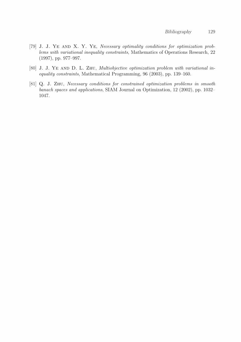
Bibliography 129

[79] J. J. Ye and X. Y. Ye, Necessary optimality conditions for optimization prob-lems with variational inequality constraints, Mathematics of Operations Research, 22(1997), pp. 977–997.

[80] J. J. Ye and D. L. Zhu, Multiobjective optimization problem with variational in-equality constraints, Mathematical Programming, 96 (2003), pp. 139–160.

[81] Q. J. Zhu, Necessary conditions for constrained optimization problems in smoothbanach spaces and applications, SIAM Journal on Optimization, 12 (2002), pp. 1032–1047.

Documents

Constraint Qualiﬁcations and Stationarity Concepts for ... · 3.2.3 Comparison between the basic CQ ... convS convex hull of the set S cl(S) ... x ≥ y componentwise comparison