Embed Size (px)
Citation preview
Constraining Particle Physics Models with
Supernovae Observations
A thesis submitted in partial fulfillment of the requirementfor the degree of Bachelor of Science with Honors in
Physics from the College of William and Mary in Virginia,
by
Keith C. Bechtol
Accepted for
Advisor: Joshua Erlich
Gina Hoatson
Christopher Carone
Nicholas Loehr
Williamsburg, VirginiaApril 30, 2007
Abstract
Three particle physics theories are evaluated based upon their consequences for cosmology.
Observations of type Ia supernovae supplied by the Supernova Legacy Survey and Hubble Space
Telescope are used to constrain the parameters of the proposed models. First, a cosmological
model incorporating photon-axion oscillations is tested. When combined with cosmic microwave
background and baryon acoustic oscillation constraints, supernovae data restricts the decay
length of photons to be greater than 7000 Mpc. Next, we consider the possibility of dust on
a negative tension brane in a Randall-Sundrum braneworld scenario. The effective equation of
state relating pressure, p, to density, ρ, for the matter on the negative tension brane would be
p = 15ρ. Letting w denote the equation of state parameter, we have w(−) = 1
5. Substances
with positive equation of state parameters are ruled out by Big Bang nucleosynthesis. However,
we find that supernovae data alone is inconsistent with the the existence of substances with
w = 15. Finally, we test the possibility of topological defects from GUT symmetry breaking.
Relics of this symmetry breaking include cosmic strings and domain walls with equation of state
parameters wCS = −
13
and wDW = −
23
respectively. For both types of topological defects, the
allowed energy density is comparable to the matter density of the Universe.
i
Acknowledgements
The author would like to thank Professor Joshua Erlich of the College of William and Mary for
describing and discussing numerous cosmology and particle physics models. This project would not
have been possible nor nearly as enjoyable without his guidance.
ii
Contents
1 Introduction 1
2 Type Ia Supernovae 1
2.1 Supernova Legacy Survey . . . . . . . . . . . . . . . . . . . . . . . . . . . . . . . . . 3
2.2 Hubble Space Telescope . . . . . . . . . . . . . . . . . . . . . . . . . . . . . . . . . . 3
3 Cosmological Models 4
4 Particle Physics Theories 9
4.1 Photon-Axion Oscillations . . . . . . . . . . . . . . . . . . . . . . . . . . . . . . . . . 9
4.2 Randall-Sundrum Braneworlds . . . . . . . . . . . . . . . . . . . . . . . . . . . . . . 12
4.3 Topological Defects . . . . . . . . . . . . . . . . . . . . . . . . . . . . . . . . . . . . . 15
5 Statistical Analysis 18
5.1 Methodology . . . . . . . . . . . . . . . . . . . . . . . . . . . . . . . . . . . . . . . . 19
5.2 Results: Photon-Axion Oscillations . . . . . . . . . . . . . . . . . . . . . . . . . . . . 22
5.3 Results: Randall-Sundrum Braneworld Scenario . . . . . . . . . . . . . . . . . . . . . 23
5.4 Results: Topological Defects . . . . . . . . . . . . . . . . . . . . . . . . . . . . . . . . 27
6 Conclusions 30
iii
1 Introduction
Many contemporary particle physics theories have far-reaching and surprising conse-
quences for other areas of physics. For example, observations of the galaxy clusters
suggest that an additional long-range force between dark matter particles may be
needed to explain rapid galactic accelerations [1]. One might wonder what role new
particles and interactions could play in the behavoir of the Universe as a whole. In
this paper, we examine three particle physics theories in the context of their implica-
tions for cosmology. The predictions of each theory will be compared to recent type
Ia supernovae observations from the Supernova Legacy Survey and the Hubble Space
Telescope. Type Ia supernovae are important astronomical events because their in-
trinsic luminosity is predictable throughout the observable Universe. Therefore, the
redshift and the apparent brightness of type Ia supernovae can provide independent
measures of cosmological distances. The combination of these two distance mea-
surements is used to study the expansion history of the Universe. Statistical anal-
yses of cosmological models including photon-axion oscillations, Randall-Sundrum
braneworlds, and topological defects from symmetry breaking will be conducted in
the following study. The reevaluation of supernovae observations in light of the new
particle physics theories will also be used to constrain cosmological parameters in each
of these cases. The fits of cosmological parameters can then be compared to observa-
tions of the cosmic microwave background radiation from the most recent Wilkinson
Microwave Anisotropy Probe (WMAP) three-year study and measurements of large
scale structure from the Sloan Digital Sky Survey (SSDS).
2 Type Ia Supernovae
Type Ia supernovae occur in binary star systems in which a white drawf star accretes
mass from its partner star, typically a red giant. When the mass of the white dwarf
1

star surpasses the Chandrasekhar mass limit of about 1.4 solar masses, a stellar explo-
sion occurs. Due to this consistent process, the intrinisic luminosities of these events
are nearly uniform throughout the observable universe because of the fixed mass of
the exploding star. The distance of type Ia supernovae can be measured using two
independent methods. First, the consistent intrinsic luminosities of these explosions
allows type Ia supernovae to be used as standard candles. The dimmer the object
appears from Earth, the greater the observing distance. For a given cosmological
model, the measured bightness of supernovae can be used to determine cosmological
distances. Secondly, the redshift of the spectra of type Ia supernovae provides in-
formation about the expansion of space between the supernovae and the Earth since
the time of the explosion. Therefore, the relationship between the observed super-
novae luminosity and redshift can be used to trace back the expansion history of the
Universe and to constrain the parameters of cosmological models.
As alluded to previously, the intrinsic luminosities of type Ia supernovae are not
completely uniform. However, the light curves of type Ia supernovae (appearent lu-
minosity as a function of time) can be used to increase the accuracy of intrinsic lumi-
nosity estimates. Supernovae brightness rises gradually and then diminishes over the
period of roughly a month. To a first approximation, only the peak luminosity is con-
sidered when determining intrinsic luminosity. The phenomenologically based Phillips
Curve uses a stretch factor to relate the time-width of light curves to the intrinsic
luminosity of the supernovae [2]. In short, supernovae events of longer duration tend
to be brighter as well. This model was empirically generated from studies of nearby
supernovae in which the observing distance could be accurately determined by other
methods such as parallax. In addition, supernovae with a bluer light sprectrum are
also intrinsically brighter. Both the brighter-slower and brighter-bluer correlataions
must be taken into account in order to accurately gauge the intrinsic luminosities of
type Ia supernovae.
2
2.1 Supernova Legacy Survey
The supernovae observations considered in this analysis are supplied by the Super-
nova Legacy Survey and the Hubble Space Telescope. The Supernova Legacy Survey
includes data from 44 nearby (z ≤ 0.125, see redshift definition equation (3.2)) and 73
high-redshift (z ≥ 0.2) type Ia supernovae [2]. The observational program consisted
of two parts. First, the MegaCam instrument of the Canada-France-Hawaii Telescope
identified supernovae and recorded light curves. Next, the Very Large Telescope and
the Gemini and Keck telescopes performed a spectroscopic follow-up of supernovae
to confirm the events and to take redshift measurements. The Supernova Legacy
Survey data set lists both the original observed magnitudes of supernovae and the
corrected magnitudes to adjust for brighter-slower and brighter-bluer effects to in-
trinsic luminosity. The parameters used in models accounting for bright-slower and
brighter-bluer correlations were fitted to light curves of nearby supernovae [2].
2.2 Hubble Space Telescope
An additional 21 type Ia supernovae discovered by the Hubble Space Telescope com-
pliment the data sample of the Supernova Legacy Survey [3]. The observations include
13 supernovae with redshift z ≥ 1. When combining data sets, the spectrophotomet-
ric systems used in each study must be considered in order to compare observed
magnitudes. Both the Supernova Legacy Survey and the Hubble Space Telescope
experiment utilized the the Vegamag photometric system and Landolt calibration
system to record their findings [2, 3]. The Vegamag photometric system selects Vega
as a reference point for all stellar magnitudes. The Landolt calibration system allows
for calibration between B, V , R, and I filter band passes. The adoption of common
spectrophotometric methods allows for the two sets of supernovae observations to be
analyzed together. With a sample of 138 type Ia supernovae observations at hand,
we now outline the basic cosmological model used to describe the overall behavoir of
3
0.2 0.4 0.6 0.8 1 1.2 1.4
36
38
40
42
44
m
z
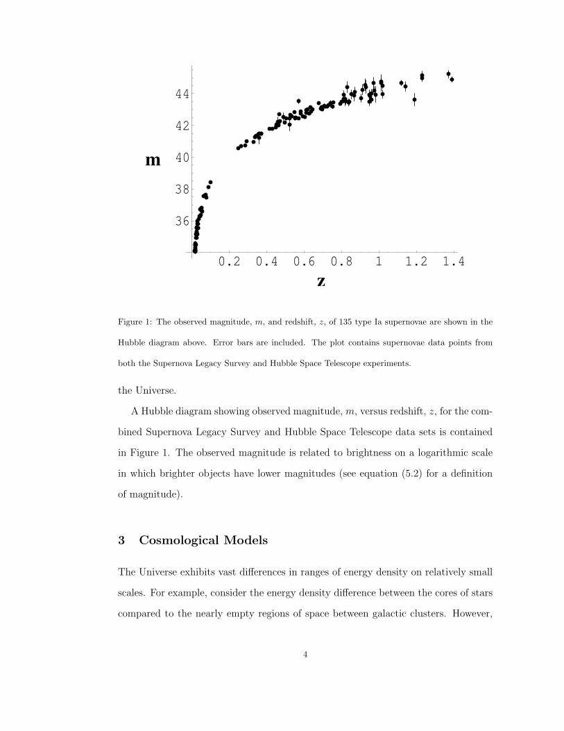
Figure 1: The observed magnitude, m, and redshift, z, of 135 type Ia supernovae are shown in the
Hubble diagram above. Error bars are included. The plot contains supernovae data points from
both the Supernova Legacy Survey and Hubble Space Telescope experiments.
the Universe.
A Hubble diagram showing observed magnitude, m, versus redshift, z, for the com-
bined Supernova Legacy Survey and Hubble Space Telescope data sets is contained
in Figure 1. The observed magnitude is related to brightness on a logarithmic scale
in which brighter objects have lower magnitudes (see equation (5.2) for a definition
of magnitude).
3 Cosmological Models
The Universe exhibits vast differences in ranges of energy density on relatively small
scales. For example, consider the energy density difference between the cores of stars
compared to the nearly empty regions of space between galactic clusters. However,
4
the combination of the Copernican Assumption (stating that there are no preferred
spatial locations) and observed isotropy (the Universe appears the same in all direc-
tions) suggests that the Universe must be homogeneous on the largest scales. The
homogeneous condition motivates the use of a maximally symmetric metric to de-
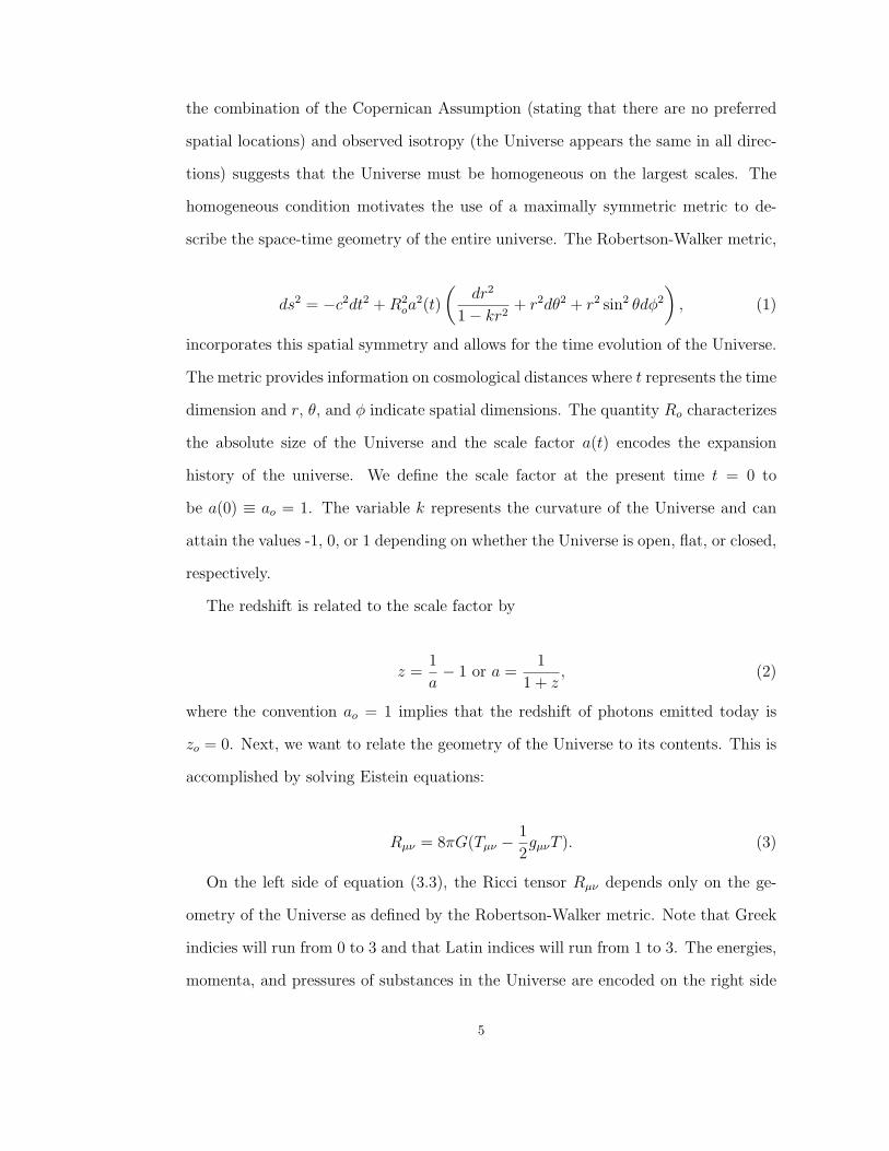
scribe the space-time geometry of the entire universe. The Robertson-Walker metric,
ds2 = −c2dt2 + R2oa
2(t)
(
dr2
1 − kr2+ r2dθ2 + r2 sin2 θdφ2
)
, (1)
incorporates this spatial symmetry and allows for the time evolution of the Universe.
The metric provides information on cosmological distances where t represents the time
dimension and r, θ, and φ indicate spatial dimensions. The quantity Ro characterizes
the absolute size of the Universe and the scale factor a(t) encodes the expansion
history of the universe. We define the scale factor at the present time t = 0 to
be a(0) ≡ ao = 1. The variable k represents the curvature of the Universe and can
attain the values -1, 0, or 1 depending on whether the Universe is open, flat, or closed,
respectively.
The redshift is related to the scale factor by
z =1
a− 1 or a =
1
1 + z, (2)
where the convention ao = 1 implies that the redshift of photons emitted today is
zo = 0. Next, we want to relate the geometry of the Universe to its contents. This is
accomplished by solving Eistein equations:
Rµν = 8πG(Tµν −1
2gµνT ). (3)
On the left side of equation (3.3), the Ricci tensor Rµν depends only on the ge-
ometry of the Universe as defined by the Robertson-Walker metric. Note that Greek
indicies will run from 0 to 3 and that Latin indices will run from 1 to 3. The energies,
momenta, and pressures of substances in the Universe are encoded on the right side
5
of Einstein’s equations. Newton’s gravitational constant is symbolized by G. We
assume that the matter and energies of cosmological interest behave as perfect fluids.
As a result of isotropy, the perfect fluids appear to be at rest in comoving coordinates
and the four-velocity can be written as Uµ = (1, 0, 0, 0), setting the speed of light
c = 1. The energy-momentum tensor Tµν = (ρ + p)UµUν + pgµν will become
Tµν =
ρ 0 0 0
0
0 gijp
0
(4)
where ρ and p indicate the pressure and density of the substances respectively and
gµν is the metric tensor. The equation of state parameter w relates the pressure and
energy density of a particular substance. Perfect fluids are described by pi = wiρi. In
addition, we have a statement for the conservation of energy,
ρi + 3(ρi + pi)H = 0 or equivalentlyρ
ρ= −3(1 + w)
a
a, (5)
because the energy-momentum tensor must be covariantly conserved. Solutions to
equation (3.5) have the form
ρi = ρi,o(1 + z)3(1+wi). (6)
For our basic cosmological model, we will consider three types of substances in
the Universe. First, matter acts as a pressureless dust with an equation of state
parameter wM = 0. Note that the vast majority of matter in the Universe exists
in the form of nonbaryonic dark matter. Next, radiation type substances such as
photons and relativistic massive particles (example: neutrinos) are described by a
traceless energy-momentum tensor in accordance with electromagnetism. The trace
of the energy-momentum tensor is T = −ρ+3p. Thus, the equation of state parameter
6
for radiation is wR = 13. Finally, the term dark energy refers to any substance with
a negative-valued equation of state parameter. Let wΛ denote the equation of state
parameter for dark energy.
The solutions to the Einstein equations using the Robertson-Walker metric and
the energy-momentum tensor given by equation (3.4) yield the Friedmann equation
H2 =
(
a
a
)2
=8πG
3c2
∑
i
ρi −kc2
a2R2o
, (7)
with the Hubble paramter defined as H ≡ aa. Next, we introduce the density param-
eter, Ω, defined as
Ωi =8πG
3H2ρi. (8)
In terms of the density parameters, the Friedmann equation can be written in a
new form in which the relationship between the sum of the density paramters and
the curvature is more evident:
∑
i
Ωi − 1 =kc2
H2a2. (9)
Define the critical density such that the spatial curvature is equal to zero when
the density parameters are summed together. This situation corresponds to a flat
Universe. We write,
Ωi =ρi
ρcrit
with ρcrit ≡3c2H2
8πG. (10)
The Friedmann equation gives the Hubble parameter in terms of the scale factor.
However, we would like to express this quantity as a function of the redshift for future
calculations. The quantity Ho indicates the Hubble Constant as determined at the
present time. The measured value for the Hubble Constant is 72 ± 5 kilometers per
second per megaparsec [4]. Substituting the redshift for the scale factor, the Hubble
parameter can now be expressed as
7
H2(z) = H2o (1 + z)2
[
1 +∑
i
Ωi
(
(1 + z)1+3wi − 1)
]
. (11)
Now consider the path of photons emitted from a distant source travelling towards
the Earth. We know that photons move along null geodesics with ds2 = 0. If the
photons propogate radially outward from the source, then we have dθ2 = 0 and
dφ2 = 0 as well. In that case, the proper time of a light ray vanishes and the
Friedmann-Robertson-Walker cosmology becomes
0 = −c2dt2 + R2oa
2(t)dr2
1 − kr2. (12)
Rearranging equation (3.12) and noting that H(z) = aa
= zz+1
= az = adzdt
, we find
that
dr√1 − kr2
=cdt
Roa(t)=
cdz
RoH(z). (13)
Integrating equation (3.13) we obtain
∫ rs
0
dr√1 − kr2
=
∫ 0
ts
cdt
Roa(t)=
∫ zs
0
cdz
RoH(z). (14)
The most recent WMAP three-year study has confirmed that the Universe appears
to be spatially flat, implying that the curvature is equal to zero [4]. After substituting
for H(z), the integral of equation (3.14) yields an equation for the comoving distance
rs(zs):
rs(zs) =c
RoHo
∫ zs
0
dz
(1 + z)√
1 +∑
i Ωi ((1 + z)1+3wi − 1). (15)
The equation for the comoving distance gives the propogation distance of photons
traveling over extragalactic distances in terms of the redshift. The absolute distance
is recovered by multiplying the comoving distance by Ro. We now have a relationship
8
between distance and redshift that depends on the cosmological density parameters
and the equation of state parameters of the contents of the Universe.
Several experimental efforts have already adressed the question of the composition
of the Universe. Using the Cosmological Concordance Model, the WMAP three-year
study found that the matter density ΩM = 0.27 ± 0.04 and that the equation of
state for dark energy wΛ = −0.98 ± 0.12 [4]. These parameter values will provide a
reference as we proceed with the analysis of particle physics theories.
4 Particle Physics Theories
Three particle physics theories will be evaluated based on how well their cosmological
implicatations match with type Ia supernovae observations. We will discuss, in order,
the theoretical background and cosmological effects of photon-axion oscillations, the
existence of shadow matter in a Randall-Sundrum braneworld scenario, and cosmic
scale topological defects from symmetry breaking.
4.1 Photon-Axion Oscillations
Supernovae observations in conjunction with contemporary cosmological models sug-
gest that the Universe is dominated by dark energy and that the expansion rate of
the Universe is accelerating exponentially [5]. However, the cosmological constant
problem motivates the search for alternative explainations for the apparent acceler-
ated expansion. The current understanding of field theory predicts a value for the
cosmological constant that is 120 orders of magnitude too large to be reconciled with
cosmology observations. Perhaps, scalar fields do not couple to gravity as expected
and do not contribute to the cosmological constant. This scenario would alleviate
the cosmological constant problem but requires a new interpretation of supernovae
data. One approach is to consider the possibility of a dimming mechanism such that
9
distant supernovae are not as bright as anticipated by traditional cosmological mod-
els. Several observations place limitations on these types of theoretical proposals.
First, the absence of significant frequency gaps or other chromatic discrepancies in
supernovae spectra requires uniform dimming across the optical range of the electro-
magnetic spectrum. This effect reduces the likelihood that light is scattered by matter
particles. Also, reemitted infrared light from interactions between photons and in-
tergalactic dust would be highly conspicuous in the cosmic microwave background
radiation [6].
A more promising dimming mechanism is a type of flavor oscillation involving
photons. To this end, Csaki, Kaloper, and Terning have proposed a model in which
photons can oscillate into axions in the presence of external magnetic fields [5, 6, 7].
According to their model, the electromagnetic field can couple with the scalar axion
field. The Lagrangian of the photon-axion interaction is given by
Lint =φ
MLc2~E · ~B, (16)
where ML signifies the coupling strength of the interaction and ~E and ~B represent
the electric and magnetic fields. Solutions to the resulting Langrange equations have
oscillatory forms in the presence of a background magnetic field. The strength of the
interactions depends on the axion mass. Historically, the axion particle was proposed
to answer the strong CP problem with a mass in the range of 10−5 eVc2
to 10−1 eVc2
.
However, the mass scale of axions in the model suggested by Csaki, Kaloper, and
Terning is closer to 10−16 eVc2
[6]. This smaller axion mass scale is chosen in order
to leave the cosmic microwave background unaffected. Notice that the existence of
an external magnetic field is required in equation (4.1) to allow for a nonzero scalar
product in the Langrangian such that mixing between photon and axion eigenstates
can occur. However, weak magnetic fields do indeed permeate the vast regions of
space between galaxies [8]. These extragalactic magnetic fields are randomly oriented
10
with domain sizes on the order of megaparsecs. Also, the field strength appears to be
relatively uniform throughout the magnetic domains. Csaki, Kaloper, and Terning
employ the approximation that photons traversing great distances will encounter
numerous magnetic domains such that the random orientations balance each other
for a net dimming effect of distant light sources [7].
In the high energy limit relevant to optical photons, both the oscillation amplitude
and oscillation length become less dependent on the specific photon energy. As a
result, the flavor mixing distributes the originally unpolarized photons evenly across
three mass eigenstates: two photon polarization states, and one axion state. Thus, the
fraction of emitted photons that remain as photons asymptotes towards 23
over large
distances [7]. After a series of calculations, Csaki, Kaloper, and Terning determine
that the survival probability of high energy photons as a function of propogation
distance can be written as
Pγ→γ(l) ∼=2
3+
1
3e−l/Ldecay , (17)
where l represents the distance traveled by photons and Ldecay denotes the decay
length of photons [6]. In the high energy limit, the decay length is approximated by
Ldecay =8
3
ℏ2c6M2
L
Ldom| ~B|2. (18)
The average intergalactic magnetic field domain size is measured to be Ldom ∼ 1Mpc
and the intergalactic magnetic field strength is roughly 10−13 tesla such that the
magnetic field strength given in units of energy squared is | ~B|2 ∼ 10−13T√
4πεoℏ3c5
[8]. As a convention in this paper, we will express the decay length as a multiple of the
theoretical decay length suggested by Csaki, Kaloper, and Terning: Lth∼= 3600Mpc
[6].
11
4.2 Randall-Sundrum Braneworlds
The Randall-Sundrum braneworld scenario proposes a new geometry to describe the
Universe. The theory is a member of the larger class of Kaluza-Klein theories that
posit the existence of extra spatial dimensions. According to Randall and Sundrum,
Standard Model physics with the exception of gravity is confined to 4-dimensional
spaces called branes embedded in a higher dimensional geometry [9]. In contrast, grav-
ity can exist everywhere in the Randall-Sundrum braneworld. The Randall-Sundrum
braneworld concept is motivated by an effort to explain the hierarchy problem in
particle physics: an issue related to the scale of new gravitational physics and the
puzzle of why gravity appears so weak in comparison to the other fundamental forces.
In the theory, there exists a more fundamental scale of new gravitational physics that
is multiplied by a factor related to brane tension and the distance between branes.
Despite our confinement on a particular brane, matter on other branes may still
interact gravitationally with matter on our brane and produce observable effects [10].
Garriga and Tanaka call this matter existing on other branes shadow matter. Gar-
riga and Tanaka study a particular braneworld scenario with one additional spatial
dimension, y, and two branes. Their model proposes that we live on a positive ten-
sion brane located at y = 0 and that a negative tension brane exists at y = d. The
five-dimensional Anti-deSitter space geometry of the braneworld is given by
ds2 = gabdxadxb = dy2 + a2(y)ηµνdxµdxν (19)
with a(y) = e−|y|/l. The four-dimensional Minkowski metric is symbolized by ηµν and
l indicates the curvature radius of Anti-deSitter space as related to brane tension.
In this geometry, the apparent four-dimensional mass scale corresponding to new
gravitational physics, M4D, is related to the fundamental mass scale, MF, by
M4D ∝ MFedl . (20)
12
Notice that as the factor edl becomes large, the apparent four-dimensional Planck
scale grows rapidly. The relative adjustment of mass scales could help explain the
hierarchy problem. The perturbed metric in this space is given by gab = gab + hab.
This perturbation can be used to determine the effect of matter and energy on the
metric and hence the effect of gravitational forces in a given metric space. In the
Newtonian limit, we identify h00 = −2Φ so that we recover Poisson’s equation for the
gravitational field: ∇2h00 = −8πGρ or ∇2Φ = 4πGρ. The gravitational interaction is
generally characterized by the zero-mode (ground state) solution to the equations of
motion with higher order modes representing corrections to the gravitational potential
[9]. By solving the equations of motion in the braneworld geometry, Garriga and
Tanaka [10] derive that the zero mode approximation to the gravitational field on
each brane will satisfy
(
1
a2¤
(4)hµν
)(±)
= −∑
σ=±
16πG(σ)
(
Tµν −1
3γµνT
)(±)
± 16πG(±)
3
sinh(d/l)
e±d/lγµνT
(±).
(21)
Garriga and Tanaka introduce G(±), a quantity related to Newton’s constant in
the new geometry by
G(±) =G5l
−1e±d/l
2 sinh(d/l), (22)
where G5 denotes the five-dimensional Newton’s constant. Also appearing in equation
(4.6) is the background spatial metric, γµν , which is defined as
γµν = e−2|y|
l ηµν . (23)
The index σ in equations (4.6) and (4.7) selects the positive (plus sign) and negative
(minus sign) tension branes. Using the theoretical framework developed by Randall,
Sundrum, Garriga, and Tanaka, we can now calculate the gravitational influence of
13
matter on the negative tension brane. First, expand equation (4.6) for d/l ≫ 1,
the case in which the distance between branes is significantly larger than the brane
tension. After performing this expansion, we find that the metric perturbation on
the positive tension brane is a solution of
1
a2¤
(4)h(+)
µν = −16πG5l−1
[
(
Tµν −1
2ηµνT
)(+)
+
(
Tµν −1
3ηµνT
)(−)
e−2dl
]
. (24)
The quantities in the parentheses marked by the plus and minus signs represent
the contributions of matter and energy on the positive and negative tension branes
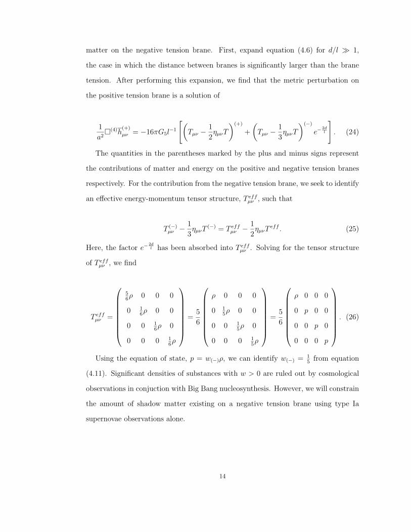
respectively. For the contribution from the negative tension brane, we seek to identify
an effective energy-momentum tensor structure, T effµν , such that
T (−)µν − 1
3ηµνT
(−) = T effµν − 1
2ηµνT
eff . (25)
Here, the factor e−2dl has been absorbed into T eff
µν . Solving for the tensor structure
of T effµν , we find
T effµν =
56ρ 0 0 0
0 16ρ 0 0
0 0 16ρ 0
0 0 0 16ρ
=5
6
ρ 0 0 0
0 15ρ 0 0
0 0 15ρ 0
0 0 0 15ρ
=5
6
ρ 0 0 0
0 p 0 0
0 0 p 0
0 0 0 p
. (26)
Using the equation of state, p = w(−)ρ, we can identify w(−) = 15
from equation
(4.11). Significant densities of substances with w > 0 are ruled out by cosmological
observations in conjuction with Big Bang nucleosynthesis. However, we will constrain
the amount of shadow matter existing on a negative tension brane using type Ia
supernovae observations alone.
14
4.3 Topological Defects
The unification of the strong, weak, and electromagnetic forces is one of the great
achievements of gauge theory. While this effect is most evident in particle acceler-
ators today, in the early history of the Universe it is believed that the fundamental
forces coupled together as a single interaction. As the Universe cooled, spontaneous
symmetry breaking may have occured as early fields froze in particular orientations
[11]. The Higgs field is one example of a field that may have acquired nonzero ex-
pectation value during this period. As the temperature decreased, the scalar field
potential transitioned from having a single minumum value to having multiple possi-
ble minima. Thus, it became possible for two neighborhing regions of space to have
differing field values corresponding to distinct ground states. The pattern of symme-
try breaking may have produced topological defects whose gravitational effects would
have cosmological consequences.
Cosmic strings and domain walls are two examples of cosmic vacuum structures
associated with symmetry breaking [11, 12]. Domain walls are the two-dimensional
structures that mark the boundaries between field domains. Cosmic strings are one-
dimensional topological defects created during a different phase transition of symme-
try breaking. In order to determine the macroscopic gravitational effects of topological
defects, we calculate the energy-momentum tensor following the method of Vilenkin
[12]. First, model a domain wall as an infinitely thin static plane located at x = a.
The energy momentum-tensor of this configuration is
T νµ (x) = δ(x − a)
∫
T νµ (x)dx, (27)
where
T νµ (x) =
∑
i
∂L
∂(∂νφ(i))∂µφ
(i) − δνµL (28)
15
for fields φ(i) and field Langragians L(φ(i), ∂µφ(i)). Note that in this geometry, the
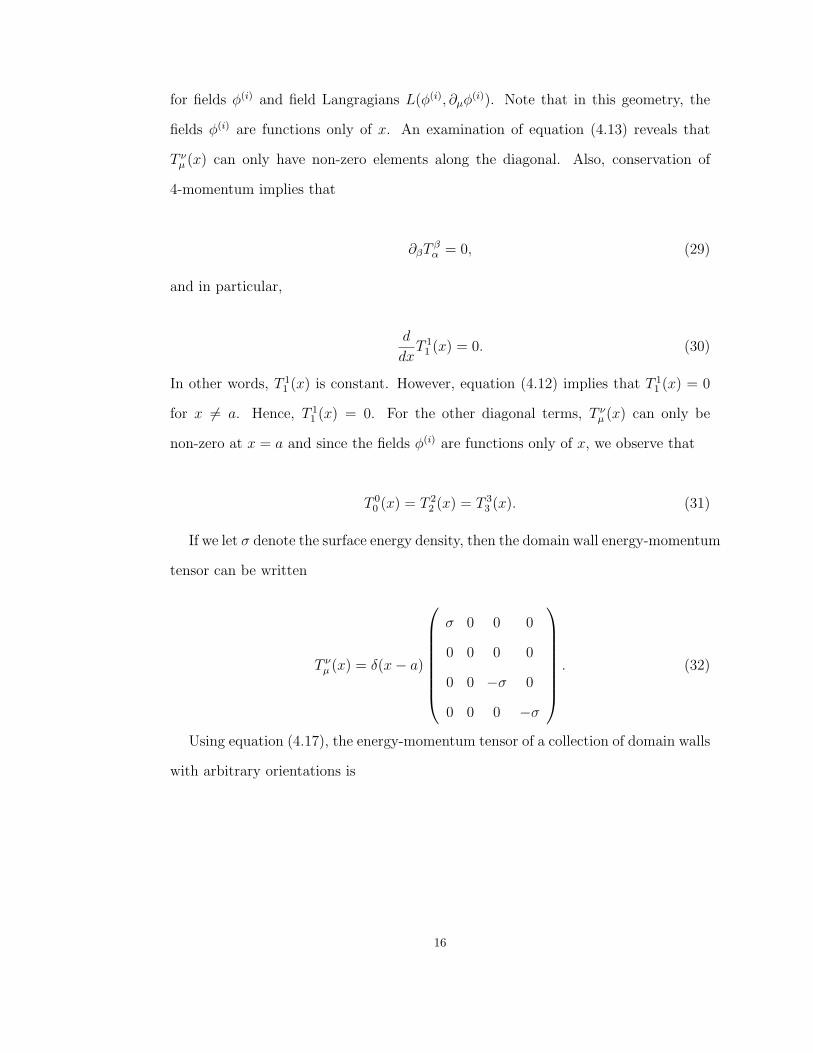
fields φ(i) are functions only of x. An examination of equation (4.13) reveals that
T νµ (x) can only have non-zero elements along the diagonal. Also, conservation of
4-momentum implies that
∂βT βα = 0, (29)
and in particular,
d
dxT 1
1 (x) = 0. (30)
In other words, T 11 (x) is constant. However, equation (4.12) implies that T 1
1 (x) = 0
for x 6= a. Hence, T 11 (x) = 0. For the other diagonal terms, T ν
µ (x) can only be
non-zero at x = a and since the fields φ(i) are functions only of x, we observe that
T 00 (x) = T 2
2 (x) = T 33 (x). (31)
If we let σ denote the surface energy density, then the domain wall energy-momentum
tensor can be written
T νµ (x) = δ(x − a)
σ 0 0 0
0 0 0 0
0 0 −σ 0
0 0 0 −σ
. (32)
Using equation (4.17), the energy-momentum tensor of a collection of domain walls
with arbitrary orientations is
16
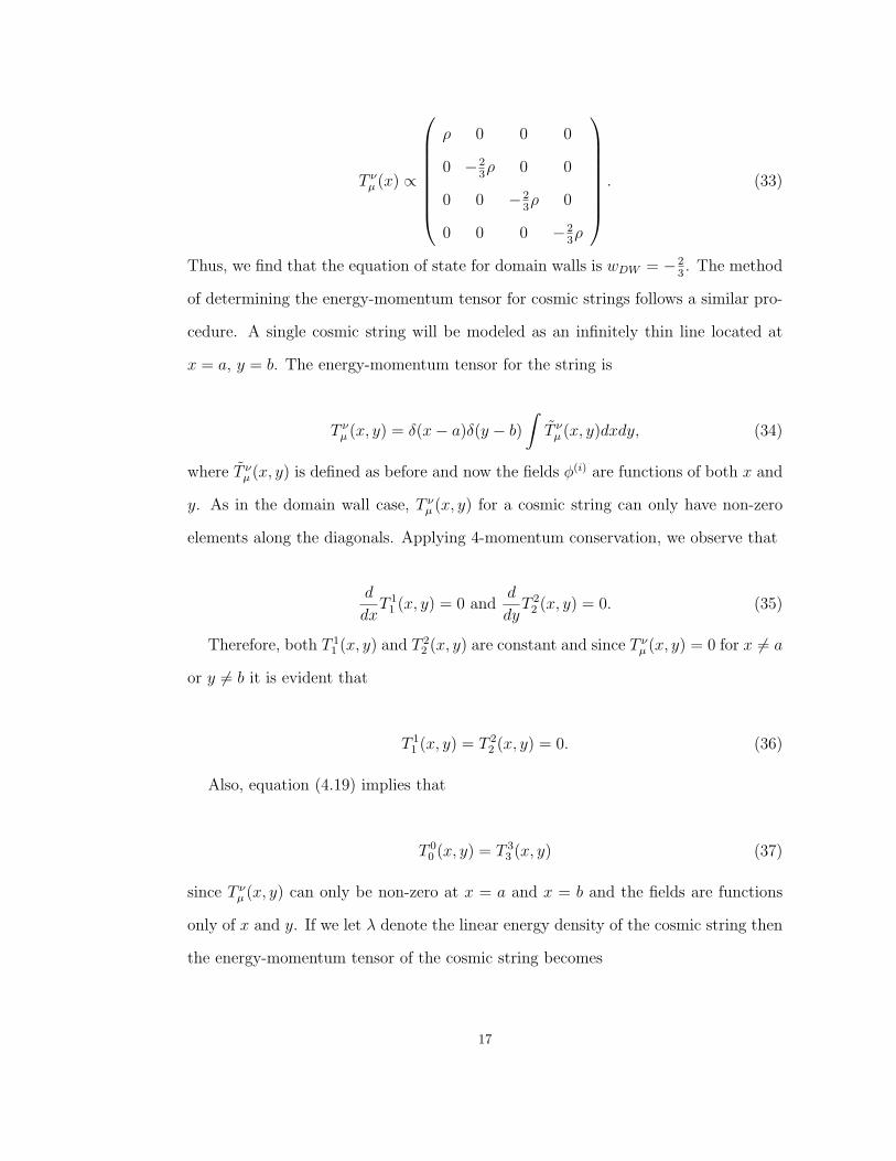
T νµ (x) ∝
ρ 0 0 0
0 −23ρ 0 0
0 0 −23ρ 0
0 0 0 −23ρ
. (33)
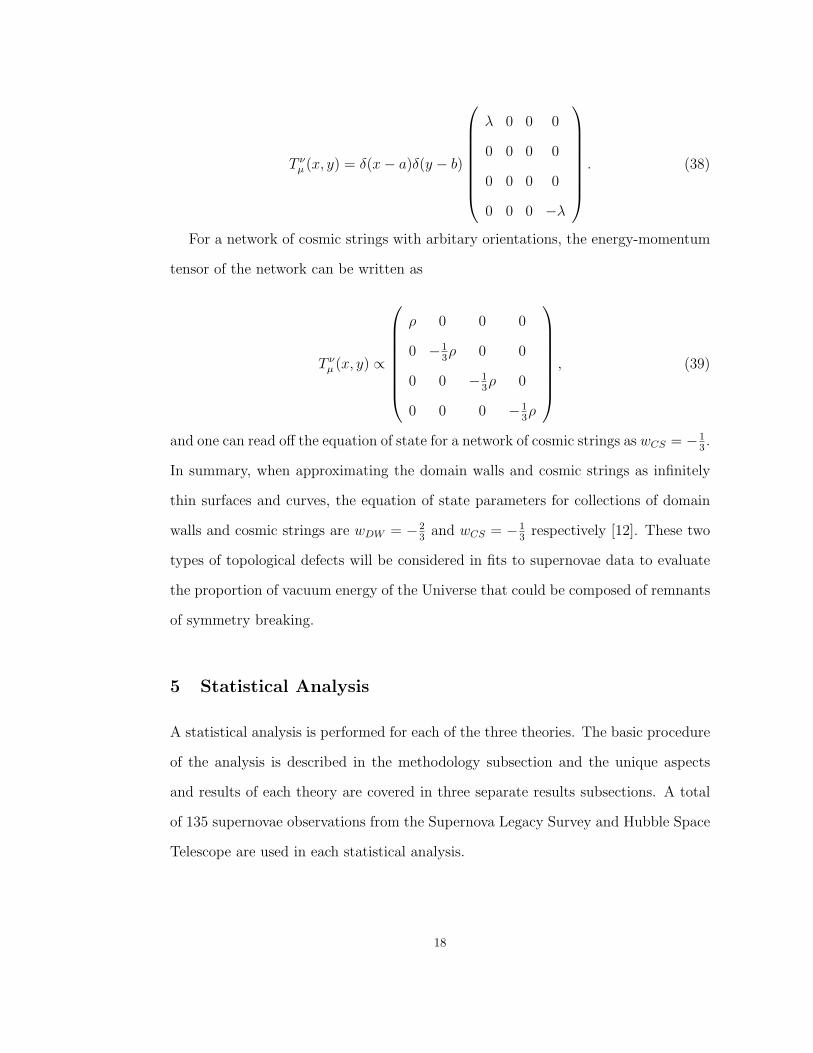
Thus, we find that the equation of state for domain walls is wDW = −23. The method
of determining the energy-momentum tensor for cosmic strings follows a similar pro-
cedure. A single cosmic string will be modeled as an infinitely thin line located at
x = a, y = b. The energy-momentum tensor for the string is
T νµ (x, y) = δ(x − a)δ(y − b)
∫
T νµ (x, y)dxdy, (34)
where T νµ (x, y) is defined as before and now the fields φ(i) are functions of both x and
y. As in the domain wall case, T νµ (x, y) for a cosmic string can only have non-zero
elements along the diagonals. Applying 4-momentum conservation, we observe that
d
dxT 1
1 (x, y) = 0 andd
dyT 2
2 (x, y) = 0. (35)
Therefore, both T 11 (x, y) and T 2
2 (x, y) are constant and since T νµ (x, y) = 0 for x 6= a
or y 6= b it is evident that
T 11 (x, y) = T 2
2 (x, y) = 0. (36)
Also, equation (4.19) implies that
T 00 (x, y) = T 3
3 (x, y) (37)
since T νµ (x, y) can only be non-zero at x = a and x = b and the fields are functions
only of x and y. If we let λ denote the linear energy density of the cosmic string then
the energy-momentum tensor of the cosmic string becomes
17
T νµ (x, y) = δ(x − a)δ(y − b)
λ 0 0 0
0 0 0 0
0 0 0 0
0 0 0 −λ
. (38)
For a network of cosmic strings with arbitary orientations, the energy-momentum
tensor of the network can be written as
T νµ (x, y) ∝
ρ 0 0 0
0 −13ρ 0 0
0 0 −13ρ 0
0 0 0 −13ρ
, (39)
and one can read off the equation of state for a network of cosmic strings as wCS = −13.
In summary, when approximating the domain walls and cosmic strings as infinitely
thin surfaces and curves, the equation of state parameters for collections of domain
walls and cosmic strings are wDW = −23
and wCS = −13
respectively [12]. These two
types of topological defects will be considered in fits to supernovae data to evaluate
the proportion of vacuum energy of the Universe that could be composed of remnants
of symmetry breaking.
5 Statistical Analysis
A statistical analysis is performed for each of the three theories. The basic procedure
of the analysis is described in the methodology subsection and the unique aspects
and results of each theory are covered in three separate results subsections. A total
of 135 supernovae observations from the Supernova Legacy Survey and Hubble Space
Telescope are used in each statistical analysis.
18
5.1 Methodology
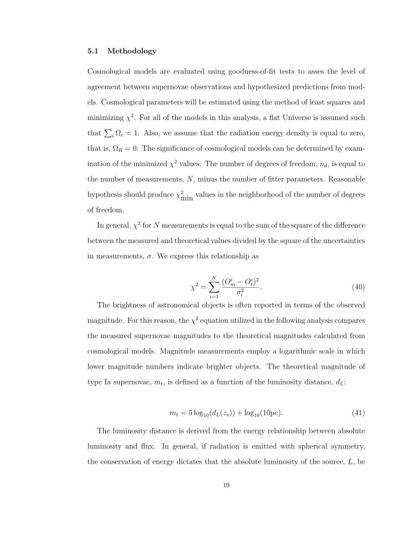
Cosmological models are evaluated using goodness-of-fit tests to asses the level of
agreement between supernovae observations and hypothesized predictions from mod-
els. Cosmological parameters will be estimated using the method of least squares and
minimizing χ2. For all of the models in this analysis, a flat Universe is assumed such
that∑
i Ωi = 1. Also, we assume that the radiation energy density is equal to zero,
that is, ΩR = 0. The significance of cosmological models can be determined by exam-
ination of the minimized χ2 values. The number of degrees of freedom, nd, is equal to
the number of measurements, N , minus the number of fitter parameters. Reasonable
hypothesis should produce χ2min values in the neighborhood of the number of degrees
of freedom.
In general, χ2 for N measurements is equal to the sum of the square of the difference
between the measured and theoretical values divided by the square of the uncertainties
in measurements, σ. We express this relationship as
χ2 =N
∑
i=1
(Oim − Oi
t)2
σ2i
. (40)
The brightness of astronomical objects is often reported in terms of the observed
magnitude. For this reason, the χ2 equation utilized in the following analysis compares
the measured supernovae magnitudes to the theoretical magnitudes calculated from
cosmological models. Magnitude measurements employ a logarithmic scale in which
lower magnitude numbers indicate brighter objects. The theoretical magnitude of
type Ia supernovae, mt, is defined as a function of the luminosity distance, dL:
mt = 5 log10(dL(zs)) + log10(10pc). (41)
The luminosity distance is derived from the energy relationship between absolute
luminosity and flux. In general, if radiation is emitted with spherical symmetry,
the conservation of energy dictates that the absolute luminosity of the source, L, be
19
related to the observed flux, F , by an inverse square law. If we treat the flux surface
as a sphere of radius d then
f
L=
1
A(d)=
1
4πd2, (42)
where A(d) denotes the area of the spherical flux surface. In the context of inter-
galactic distances, we set d = rsRo. The comoving distance from equation (3.15) is
scaled by the absolute size of the Universe. However, the expansion of the Universe
introduces two factors of (1 + zs) into the energy relationship of equation (5.3). One
factor accounts for the energy loss of photons as the wavelength increases due to the
expansion of space. Recall that the photon energy, E, depends on the wavelength,
λ, according to the equation E = hc/λ. Additionally, individual photons emitted by
the source arrive at the flux surface with a frequency reduced by a factor of (1 + zs).
Thus,
L = 4πr2sR
2o(1 + zs)
2F. (43)
The luminosity distance is defined such that L = 4πd2LF . Consequently, the lumi-
nosity distance can be expressed as a function of redshift. For traditional cosmological
models, we have
dL = (1 + zs)rs(zs)Ro. (44)
As previously mentioned, the χ2 equation compares the observed supernovae mag-
nitudes to the theoretical magnitudes calculated with various cosmological models.
The observed supernovae magnitudes, µB, have been previously corrected to account
for brighter-slower and brighter-bluer correlations in the Supernova Legacy Survey [2].
The quantities σ(µB) and σint denote the uncertainties associated with supernovae
magnitude measurements and theoretical uncertainties in determining the intrinsic
20
luminosity of type Ia supernovae. Subsequent calculations set the theoretical dis-
persion uncertainty to σint = 0.13 in accordance with the Supernova Legacy Survey
analysis [2]. After a series of substitutions, we develop a new χ2 equation:
χ2 =∑
objects
(µB − 5 log10(dL(zs)) + log10(10pc) + δM)2
σ2(µB) + σ2int
. (45)
The values of χ2 prove to be extremely sensitive to the absolute magnitude used
when calculating µB. Therefore, an additional paramter, δM , has been included in the
χ2 equation to assess the absolute magnitude scale difference between observation and
theory. If the absolute magnitude scale used to calibrate values of µB corresponds
closely to the reference magnitude used to calculate mt, then we expect the fitted
values of δM to be small for minimized χ2.
For each particle physics theory, χ2 is minimized numerically with respect to the
relevant cosmological parameters. Next, confidence plots are created to illustrate the
most probable regions of parameter space. Assuming that a given theory is correct,
confidence plots show lines of equal probability that the actual parameter values of
the Universe lie within a selected region of parameter space. The confidence intervals
are generated by contours of one minus the p-value of the hypothesis:
1 − p = 1 −∫ ∞
∆χ2(pj)
f(x, n)dx. (46)
The value of ∆χ2 as a function of fitted parameters pj is defined to be the difference
between χ2 evaluated at pj and the minimized value of χ2. We define
∆χ2(pj) ≡ χ2(pj) − χ2min. (47)
The probability density function, f(x, n), for χ2 tests with n degrees of freedom is
given by
21
f(x, n) =x
n2−1e−
x2
2n2 Γ(n
2)
. (48)
The resulting tables of minimized χ2 values and associated cosmological parameter
values are contained in the results subsection for each theory. Relevant confidence
plots are also included in each of the results subsections.
5.2 Results: Photon-Axion Oscillations
The inclusion of photon-axion oscillations modifies the luminosity-flux energy rela-
tionship given by equation (5.4) by removing a fraction of the photons arriving at the
flux surface. The luminosity-flux relationship becomes
L =4πr2
sR2o(1 + zs)
2F
Pγ→γ(rs(zs)Ro). (49)
Now the luminosity distance is reduced by the square root of the survival proba-
bility of photons. For photon-axion oscillations we have
dL =(1 + zs)rs(zs)Ro
P1/2γ→γ(rs(zs)Ro)
. (50)
In a first round of tests, χ2 is minimized with respect to wΛ, ΩM , and δM for
a Universe without photon axion oscillations. Our flat Universe assumption implies
that ΩM +ΩΛ = 1. To include the possibility of photon-axion oscillations, χ2 is mini-
mized with respect to the additional decay length parameter, Ldec. The decay length
parameter, Ldec, is a dimensionless scale factor such that the actual decay length of
photons is equal to the product of Ldec and the theoretical decay length calculated by
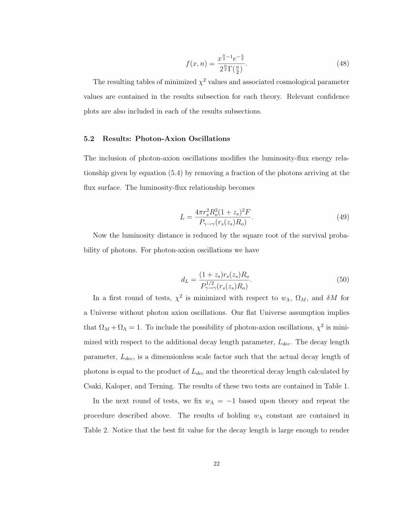
Csaki, Kaloper, and Terning. The results of these two tests are contained in Table 1.
In the next round of tests, we fix wΛ = −1 based upon theory and repeat the
procedure described above. The results of holding wΛ constant are contained in
Table 2. Notice that the best fit value for the decay length is large enough to render
22
Control Oscillations
χ2 177.5 177.5
wΛ -0.670 -0.915
ΩM 0.192 0.256
δM -0.002 -0.002
Ldec 1.04 Lth
Table 1: The best fit for the photon-axion oscillations model is compared to a control case with
no oscillations. The minimized χ2 value and best fit cosmological parameters are shown above.
The values were determined from 135 measurements of nearby and high-redshift type Ia supernovae
(N = 135). Lth denotes the theoretical decay length of photons as predicted by Csaki, Kaloper, and
Terning. Accordingly, we set Lth = 3600Mpc [6].
the effect of photon-axion oscillations negligible. Figures 2 and 3 contain confidence
plots comparing the most probable values of cosmological parameters for models with
and without photon-axion oscillations respectively.
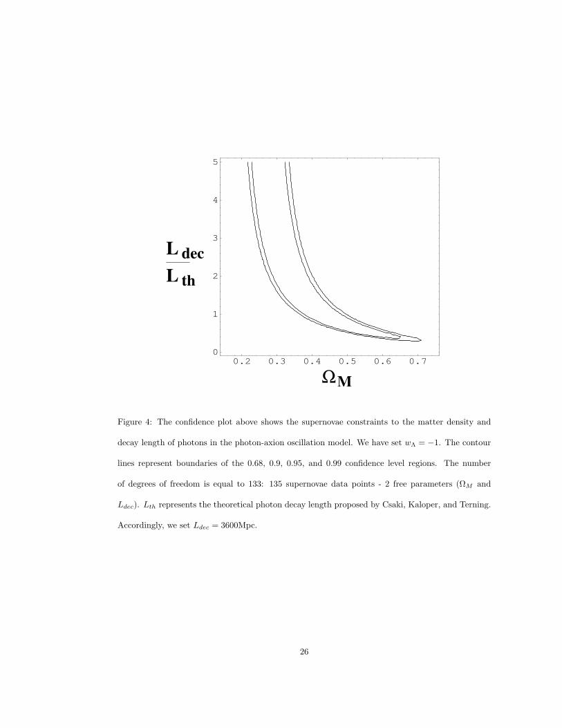
A final confidence plot showing the supernovae constraints on the matter density
and photon decay length is contained in Figure 4. In this plot, we have set wΛ =
−1. The region of high probability in parameter space shown in Figure 4 continues
vertically off the figure as Ldec
Lthbecomes significantly greater than one. Recall from
Table 2 that the best fit of parameters to supernovae data is located at ΩM = 0.223,
Ldec = 113.
5.3 Results: Randall-Sundrum Braneworld Scenario
In the Randall-Sundrum braneworld scenario we can use the luminosity distance
from equation (5.5) but now we add the possibility of shadow matter on the negative
tension brane. The equation for a flat cosmology now becomes
23
0 0.2 0.4 0.6 0.8 1
-1
-0.5
0
0.5
1
Μ
Λw
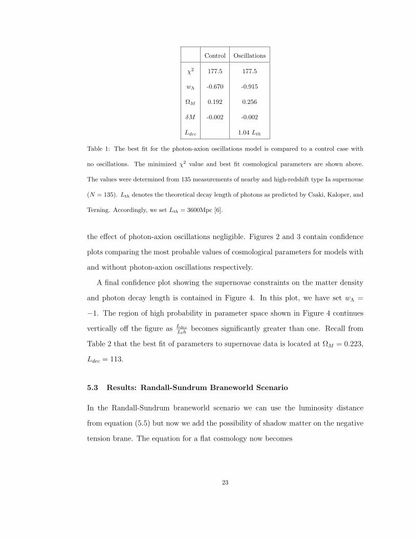
Ω
Figure 2: A confidence plot including photon-axion oscillations is shown above. The shaded regions
indicate regions of parameter space where cosmological parameters as most likely to be located.
The contour lines represent boundaries of the 0.68, 0.9, 0.95, and 0.99 confidence level regions. The
number of degrees of freedom is equal to 133: 135 supernovae data points - 2 free parameters (ΩM
and wΛ). We have set the photon decay length equal to the theoretical decay length suggested by
Csaki, Kaloper, and Terning in the above plot above [6]. That is, Ldec = Lth = 3600Mpc.
24
0 0.2 0.4 0.6 0.8 1
-1
-0.5
0
0.5
1
Μ
Λw
Ω
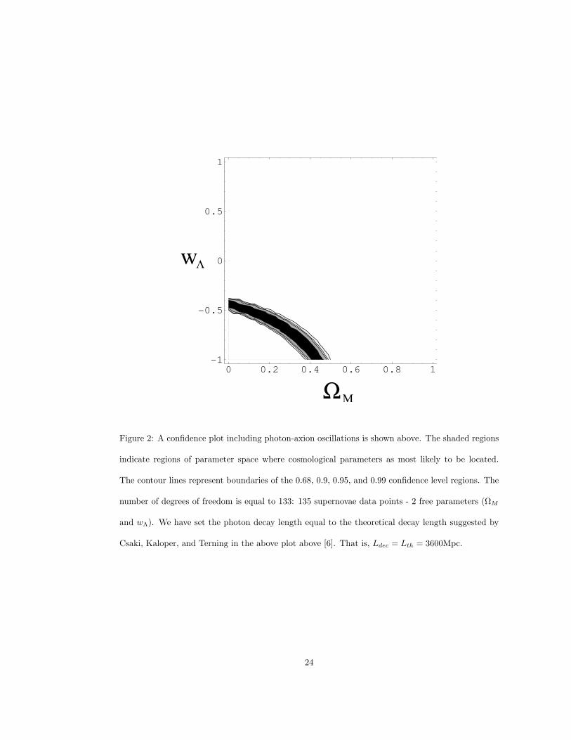
Figure 3: A confidence plot without photon-axion oscillations is shown above as a comparison to
Figure 2. The shaded regions indicate regions of parameter space where cosmological parameters
as most likely to be located. The contour lines represent boundaries of the 0.68, 0.9, 0.95, and 0.99
confidence level regions. The number of degrees of freedom is equal to 133: 135 supernovae data
points - 2 free parameters (ΩM and wΛ).
25
0.2 0.3 0.4 0.5 0.6 0.7
0
1
2
3
4
5
thL
decL
ΩM
Figure 4: The confidence plot above shows the supernovae constraints to the matter density and
decay length of photons in the photon-axion oscillation model. We have set wΛ = −1. The contour
lines represent boundaries of the 0.68, 0.9, 0.95, and 0.99 confidence level regions. The number
of degrees of freedom is equal to 133: 135 supernovae data points - 2 free parameters (ΩM and
Ldec). Lth represents the theoretical photon decay length proposed by Csaki, Kaloper, and Terning.
Accordingly, we set Ldec = 3600Mpc.
26
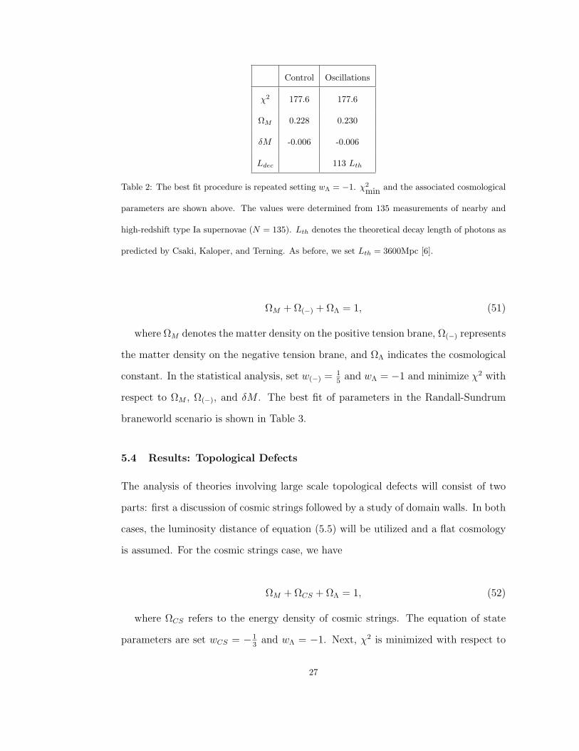
Control Oscillations
χ2 177.6 177.6
ΩM 0.228 0.230
δM -0.006 -0.006
Ldec 113 Lth
Table 2: The best fit procedure is repeated setting wΛ = −1. χ2min and the associated cosmological
parameters are shown above. The values were determined from 135 measurements of nearby and
high-redshift type Ia supernovae (N = 135). Lth denotes the theoretical decay length of photons as
predicted by Csaki, Kaloper, and Terning. As before, we set Lth = 3600Mpc [6].
ΩM + Ω(−) + ΩΛ = 1, (51)
where ΩM denotes the matter density on the positive tension brane, Ω(−) represents
the matter density on the negative tension brane, and ΩΛ indicates the cosmological
constant. In the statistical analysis, set w(−) = 15
and wΛ = −1 and minimize χ2 with
respect to ΩM , Ω(−), and δM . The best fit of parameters in the Randall-Sundrum
braneworld scenario is shown in Table 3.
5.4 Results: Topological Defects
The analysis of theories involving large scale topological defects will consist of two
parts: first a discussion of cosmic strings followed by a study of domain walls. In both
cases, the luminosity distance of equation (5.5) will be utilized and a flat cosmology
is assumed. For the cosmic strings case, we have
ΩM + ΩCS + ΩΛ = 1, (52)
where ΩCS refers to the energy density of cosmic strings. The equation of state
parameters are set wCS = −13
and wΛ = −1. Next, χ2 is minimized with respect to
27
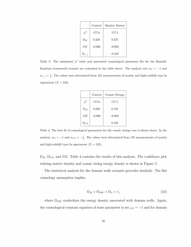
Control Shadow Matter
χ2 177.6 177.5
ΩM 0.228 0.375
δM -0.006 -0.002
Ω(−) -0.104
Table 3: The minimized χ2 value and associated cosmological parameter fits for the Randall-
Sundrum braneworld scenario are contained in the table above. The analysis sets wΛ = −1 and
w(−) = 15 . The values were determined from 135 measurements of nearby and high-redshift type Ia
supernovae (N = 135).
Control Cosmic Strings
χ2 177.6 177.5
ΩM 0.228 0.135
δM -0.006 -0.002
ΩCS 0.180
Table 4: The best fit of cosmological parameters for the cosmic strings case is shown above. In the
analysis, wΛ = −1 and wCS = − 13 . The values were determined from 135 measurements of nearby
and high-redshift type Ia supernovae (N = 135).
ΩM , ΩCS, and δM . Table 4 contains the results of this analysis. The confidence plot
relating matter density and cosmic string energy density is shown in Figure 5.
The statistical analysis for the domain walls scenario procedes similarly. The flat
cosmology assumption implies
ΩM + ΩDW + ΩΛ = 1, (53)
where ΩDW symbolizes the energy density associated with domain walls. Again,
the cosmological constant equation of state parameter is set ωΛ = −1 and for domain
28
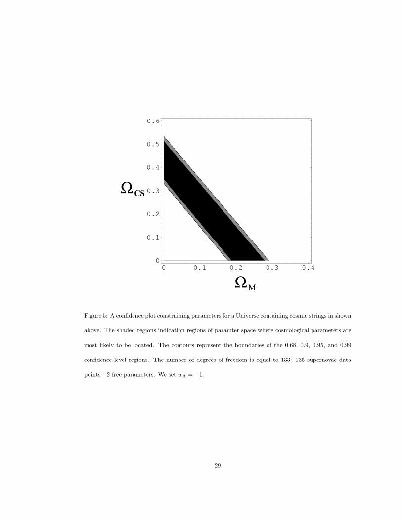
0 0.1 0.2 0.3 0.4
0
0.1
0.2
0.3
0.4
0.5
0.6
Μ
CS
Ω
Ω
Figure 5: A confidence plot constraining parameters for a Universe containing cosmic strings in shown
above. The shaded regions indication regions of paramter space where cosmological parameters are
most likely to be located. The contours represent the boundaries of the 0.68, 0.9, 0.95, and 0.99
confidence level regions. The number of degrees of freedom is equal to 133: 135 supernovae data
points - 2 free parameters. We set wΛ = −1.
29
Control Domain Walls
χ2 177.6 177.5
ΩM 0.228 0.180
δM -0.006 -0.002
ΩDW 0.234
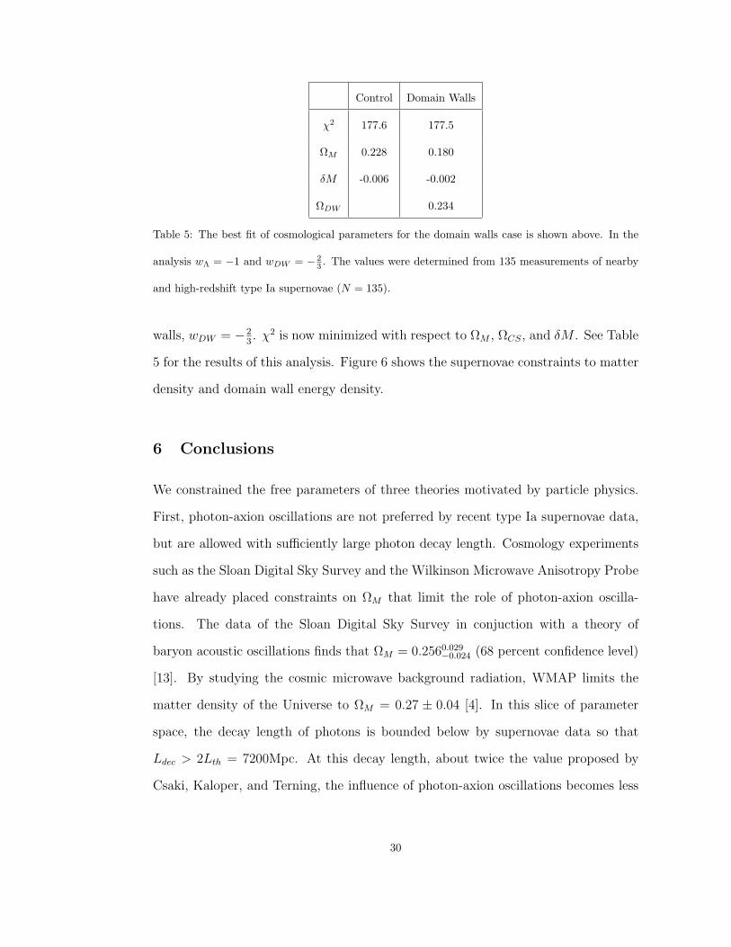
Table 5: The best fit of cosmological parameters for the domain walls case is shown above. In the
analysis wΛ = −1 and wDW = − 23 . The values were determined from 135 measurements of nearby
and high-redshift type Ia supernovae (N = 135).
walls, wDW = −23. χ2 is now minimized with respect to ΩM , ΩCS, and δM . See Table
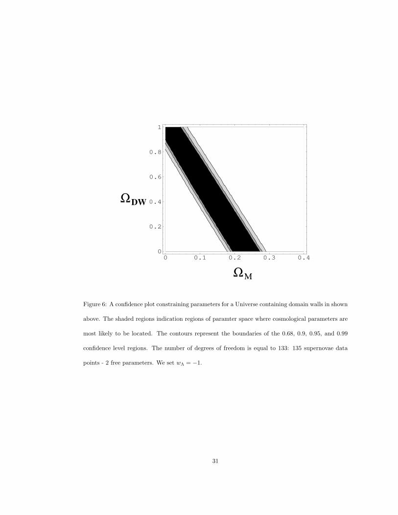
5 for the results of this analysis. Figure 6 shows the supernovae constraints to matter
density and domain wall energy density.
6 Conclusions
We constrained the free parameters of three theories motivated by particle physics.
First, photon-axion oscillations are not preferred by recent type Ia supernovae data,
but are allowed with sufficiently large photon decay length. Cosmology experiments
such as the Sloan Digital Sky Survey and the Wilkinson Microwave Anisotropy Probe
have already placed constraints on ΩM that limit the role of photon-axion oscilla-
tions. The data of the Sloan Digital Sky Survey in conjuction with a theory of
baryon acoustic oscillations finds that ΩM = 0.2560.029−0.024 (68 percent confidence level)
[13]. By studying the cosmic microwave background radiation, WMAP limits the
matter density of the Universe to ΩM = 0.27 ± 0.04 [4]. In this slice of parameter
space, the decay length of photons is bounded below by supernovae data so that
Ldec > 2Lth = 7200Mpc. At this decay length, about twice the value proposed by
Csaki, Kaloper, and Terning, the influence of photon-axion oscillations becomes less
30
0 0.1 0.2 0.3 0.4
0
0.2
0.4
0.6
0.8
1
Μ
DWΩ
Ω
Figure 6: A confidence plot constraining parameters for a Universe containing domain walls in shown
above. The shaded regions indication regions of paramter space where cosmological parameters are
most likely to be located. The contours represent the boundaries of the 0.68, 0.9, 0.95, and 0.99
confidence level regions. The number of degrees of freedom is equal to 133: 135 supernovae data
points - 2 free parameters. We set wΛ = −1.
31
significant. However, photon-axion oscillations are still important to consider be-
cause if new cosmological experiments discover that ΩM > 0.4, then photon-axion
oscillations are strongly perferred by type Ia supernovae data.
The supernovae data also confirms that substances with positive equation of state
parameters are not allowed given our current understanding of cosmology. In the
case of shadow matter on a negative tension brane with w(−) = 15, no density value
of shadow matter improves the fit to supernovae data.
Finally, we examined the possibility that some component of the dark energy is
composed of topological defects such as a network of cosmic strings or domain walls
with equation of state parameters wCS = −13
and wDW = −23
respectively. We
assumed that wΛ = −1. When combining the analysis of type Ia supernovae data
with studies of baryon acoustic oscillations and the cosmic microwave background, we
find that 0.0 < ΩCS < 0.1 and 0.0 < ΩDW < 0.2 at the 68 percent confidence level.
Thus, type Ia supernovae observations allow a density of domain walls comparable to
the component of dark matter in the Universe.
References
[1] G.R. Farrar, R.A. Rosen, A New Force in the Dark Sector?, Phys. Rev. Lett.
(2006), astro-ph/0610298.
[2] P. Astier, et al., The Supernova Legacy Survey: Measurement of ΩM , ΩΛ, and
ω from the First Year Data Set, Astronomy and Astrophysics 447 (2006) 31,
astro-ph/0510447.
[3] A.G. Riess, et al., New Hubble Space Telescope Discoveries of Type Ia Super-
novae at z > 1: Narrowing Constraints on the Early Behavior of Dark Energy,
Astrophysics Journal 656 (2006), astro-ph/0611572.
32
[4] D. Spergel, et al., First Year Wilkinson Microwave Anisotropy Probe (WMAP)
Observations: Determination of Cosmological Parameters, Astrophys. J. Suppl.
148 (2003) 175, astro-ph/0302209.
[5] C. Csaki, N. Kaloper, J. Terning, The accelerated acceleration of the universe,
JCAP 0606 (2006) 022, astro-ph/0507148.
[6] C. Csaki, N. Kaloper, J. Terning, Dimming supernovae without cosmic accelera-
tion, Phys. Rev. Lett. 88 (2002) 161302, hep-ph/0111311.
[7] C. Csaki, N. Kaloper, J. Terning, Effects of the intergalactic plasma on su-
pernova dimming via photon axion oscillations, Phys. Lett. B535 (2002) 33,
hep-ph/0112212.
[8] K. Jedamzik, V. Katalinic, A.V. Olinto, A Limit on Primordial Small-Scale
Magnetic Fields from CMB Distortions, Phys. Rev. Lett. 85 (2000) 700,
astro-ph/9911100.
[9] C. Csaki, J. Erlich, T.J. Hollowood, Y. Shirman, Universal Aspects of Gravity
Localized on Thick Branes, Nucl. Phys. B581 (2000) 309, hep-th/0001033.
[10] J. Garriga, T. Tanaka, Gravity in the Randall-Sundrum Brane World, Phys. Rev.
Lett. 84 (2000) 2778, hep-th/9911055.
[11] A. Vilenkin, Cosmic Strings and Other Topological Defects, Cambridge Univer-
sity Press, Cambridge, 1994.
[12] A. Vilenkin, Gravitational field of vacuum domain walls and strings, Phys. Rev.
D23 (1981) 852.
[13] W. Percival, Measuring the matter density using Baryon Accoustic Oscillations
in the SSDS, ApJ (2006), astro-ph/0608365v2.
33