Constrained Semi-supervised Learning in thePresence of Unanticipated Classes

Bhavana Bharat Dalvibbd@cs.cmu.edu

CMU-LTI-15-006

Language Technologies InstituteSchool of Computer ScienceCarnegie Mellon University

5000 Forbes Ave., Pittsburgh, PA 15213www.lti.cs.cmu.edu

Thesis Committee:Prof. William W. Cohen (Co-Chair), Carnegie Mellon University

Prof. Jamie Callan (Co-Chair), Carnegie Mellon UniversityProf. Tom Mitchell, Carnegie Mellon University

Dr. Alon Halevy, Google Research

Submitted in partial fulfillment of the requirementsfor the degree of Doctor of Philosophy

In Language and Information Technologies.

Copyright c© 2015 Bhavana Bharat Dalvibbd@cs.cmu.edu

Keywords: Semi-supervised learning, Clustering, New class discovery, Knowledge bases,Ontologies, Entities on the Web, Multi-view Learning

Dedicated to my beloved parents Mr. Bharat Madhav Dalvi and Mrs. Bhakti Bharat Dalvi.

iv

AcknowledgmentsThe process of PhD is challenging in many ways, and it would have been impossible to

survive without invaluable support from everyone around me. This is a heartfelt attempt toexpress my gratitude to everyone who helped me during this journey.

First and foremost, I would like to thank my advisors Prof. William W. Cohen andProf. Jamie Callan for their extensive support, and patient guidance over past six years.They always listened to my ideas carefully, however crazy they were. I have learned a lotfrom them over these years. Prof. Cohen set an example for all of us by being an awesomeresearcher, advisor, teacher, and a kind person. I like his way of putting research projectsin broad context. His encouraging words and optimism made me feel good about myselfduring difficult times in PhD. He was always approachable whenever I needed any guidance.I will always keep in mind the way he perfectly manages his professional, and personallife. I am equally thankful to Prof. Callan for co-advising my thesis. His questions duringweekly meetings always challenged me and helped me keep on track and discover mistakesquickly. He has taught me to think deeply about research problems, and to always meaning-fully question and challenge one’s own work. I deeply admire his presentation and teachingskills.

I would also like to thank my other thesis committee members Prof. Tom Mitchell,Dr. Alon Halevy. I am grateful to Prof. Tom Mitchell for his valuable comments on myresearch during NELL group meetings. I am amazed at his breadth of knowledge and enthu-siasm. The brainstorming sessions headed by Prof. Mitchell have helped me a lot in comingup with novel ideas. I sincerely thank Dr. Alon Halevy for readily agreeing to serve as theexternal member of my thesis committee, for diligently reading my drafts), and providingfeedback. I am thankful to Dr. Halevy and Dr. Anish Das Sarma for their mentorship duringmy internship at Google Research.

My sincere thanks to my family members especially my parents, husband (Aditya Mishra),and in laws. I am eternally grateful to my parents for giving me unconditional love and sup-port throughout my life. Their continuous care and love made me survive during the thickand thin. They always put my interests above theirs and imbibed in me the importance ofeducation. Aditya, has been beside me during this long journey through grad school. Hepatiently listened to my ideas, questions, and concerns and always gave me most pertinentadvice. He was always available whenever I needed him. For that, no amount of gratitudecan suffice. His optimism, relentless support and love keeps me going. I am equally gratefulto my in laws for encouraging me to continue my research work during the post marriageyears. They always lifted my spirits which helped me give my best at research.

I would also like to thank my friends Anjali, Archna, Athula, Derry, Kriti, Meghana,Naman, Pallavi, Prasanna, Ramnath, Ranjani, Reyyan, Rose, Ruta, Sunayana, Siddharth andSubhodeep for their constant support during these years. They provided a stimulating en-vironment making my graduate student life enjoyable and truly memorable. I would alsolike to thank members of the NELL group and Prof. Callan’s group for the countless thoughtprovoking conversations during the group meetings. Finally my heartfelt thanks to StaceyYoung, Sharon Cavlovich, Sandra Winkler, and the rest of the staff at CMU for their invalu-able help and assistance over the years.

vi

AbstractTraditional semi-supervised learning (SSL) techniques consider the missing la-

bels of unlabeled datapoints as latent/unobserved variables, and model these vari-ables, and the parameters of the model, using techniques like Expectation Maximiza-tion (EM). Such semi-supervised learning techniques are widely used for AutomaticKnowledge Base Construction (AKBC) tasks.

We consider two extensions to traditional SSL methods which make it more suit-able for a variety of AKBC tasks. First, we consider jointly assigning multiple labelsto each instance, with a flexible scheme for encoding constraints between assignedlabels: this makes it possible, for instance, to assign labels at multiple levels froma hierarchy. Second, we account for another type of latent variable, in the form ofunobserved classes. In open-domain web-scale information extraction problems, itis an unrealistic assumption that the class ontology or topic hierarchy we are usingis complete. Our proposed framework combines structural search for the best classhierarchy with SSL, reducing the semantic drift associated with erroneously group-ing unanticipated classes with expected classes. Together, these extensions allow asingle framework to handle a large number of knowledge extraction tasks, includingmacro-reading, noun-phrase classification, word sense disambiguation, alignment ofKBs to wikipedia or on-line glossaries, and ontology extension.

To summarize, this thesis argues that many AKBC tasks which have previouslybeen addressed separately can be viewed as instances of single abstract problem:multiview semi-supervised learning with an incomplete class hierarchy. In this thesiswe present a generic EM framework for solving this abstract task.

viii

Contents

1 Introduction 11.1 Thesis Contributions . . . . . . . . . . . . . . . . . . . . . . . . . . . . . . . . 2

1.1.1 Semi-supervised Learning in the Presence of Unanticipated Classes . . . 21.1.2 Semi-supervised Learning with Multi-view Data . . . . . . . . . . . . . 31.1.3 Semi-supervised Learning in the Presence of Ontological Constraints . . 31.1.4 Combinations of Scenarios . . . . . . . . . . . . . . . . . . . . . . . . . 4

1.2 Thesis Statement . . . . . . . . . . . . . . . . . . . . . . . . . . . . . . . . . . 41.3 Additional Potential Applications . . . . . . . . . . . . . . . . . . . . . . . . . . 51.4 Thesis Outline . . . . . . . . . . . . . . . . . . . . . . . . . . . . . . . . . . . . 6

2 Background 72.1 Information Extraction . . . . . . . . . . . . . . . . . . . . . . . . . . . . . . . 72.2 Building Knowledge Bases . . . . . . . . . . . . . . . . . . . . . . . . . . . . . 82.3 NELL: Never Ending Language Learning . . . . . . . . . . . . . . . . . . . . . 9

3 Case Study: Table Driven Information Extraction 113.1 WebSets: Unsupervised Concept-Instance Pair Extraction from HTML Tables . . 11

3.1.1 Proposed Method . . . . . . . . . . . . . . . . . . . . . . . . . . . . . . 123.1.2 Experimental Results . . . . . . . . . . . . . . . . . . . . . . . . . . . . 163.1.3 Application: Summary of the Corpus . . . . . . . . . . . . . . . . . . . 22

3.2 Related Work: IE from Tables, Semi-supervised Learning . . . . . . . . . . . . . 223.3 Semi-supervised Bottom-Up Clustering to Extend the

NELL Knowledge Base . . . . . . . . . . . . . . . . . . . . . . . . . . . . . . . 253.3.1 Semi-supervised WebSets . . . . . . . . . . . . . . . . . . . . . . . . . 253.3.2 Experimental Evaluation using NELL . . . . . . . . . . . . . . . . . . . 25

3.4 Lessons Learned from WebSets . . . . . . . . . . . . . . . . . . . . . . . . . . . 29

4 Exploratory Learning: Semi-supervised Learning in the Presence of UnanticipatedClasses 334.1 Exploratory EM Algorithm . . . . . . . . . . . . . . . . . . . . . . . . . . . . . 33

4.1.1 Discussion . . . . . . . . . . . . . . . . . . . . . . . . . . . . . . . . . 344.1.2 Model Selection . . . . . . . . . . . . . . . . . . . . . . . . . . . . . . 364.1.3 Exploratory EM using Different Language Models . . . . . . . . . . . . 364.1.4 Strategies for Inducing New Clusters/Classes . . . . . . . . . . . . . . . 37

ix

4.2 Experimental Results: Entity Clustering and Document Classification . . . . . . 384.3 Evaluation on Non-seed Classes . . . . . . . . . . . . . . . . . . . . . . . . . . 414.4 Additional Results . . . . . . . . . . . . . . . . . . . . . . . . . . . . . . . . . 414.5 Experiments with Chinese Restaurant Process . . . . . . . . . . . . . . . . . . . 434.6 Related Work: Semi-supervised Learning, Negative Class Discovery, Topic De-

tection and Tracking . . . . . . . . . . . . . . . . . . . . . . . . . . . . . . . . 494.7 Conclusion . . . . . . . . . . . . . . . . . . . . . . . . . . . . . . . . . . . . . 514.8 Future Research Directions . . . . . . . . . . . . . . . . . . . . . . . . . . . . . 51

5 Constrained Semi-supervised Learning with Multi-view Datasets 535.1 Motivation . . . . . . . . . . . . . . . . . . . . . . . . . . . . . . . . . . . . . . 535.2 Multi-View Semi-supervised Learning . . . . . . . . . . . . . . . . . . . . . . . 55

5.2.1 Background and Notation . . . . . . . . . . . . . . . . . . . . . . . . . 555.2.2 Multi-View K-Means . . . . . . . . . . . . . . . . . . . . . . . . . . . . 565.2.3 Cluster Assignment using Scores from Two Data Views . . . . . . . . . 57

5.3 Datasets and Experimental Methodology . . . . . . . . . . . . . . . . . . . . . . 595.3.1 Datasets . . . . . . . . . . . . . . . . . . . . . . . . . . . . . . . . . . . 595.3.2 Experimental Setting . . . . . . . . . . . . . . . . . . . . . . . . . . . . 605.3.3 Evaluation Criteria . . . . . . . . . . . . . . . . . . . . . . . . . . . . . 61

5.4 Experimental Results . . . . . . . . . . . . . . . . . . . . . . . . . . . . . . . . 625.4.1 Comparison of Multi-view Learning Methods in Terms of F1 . . . . . . . 625.4.2 Analysis of Results . . . . . . . . . . . . . . . . . . . . . . . . . . . . . 63

5.5 Related Work . . . . . . . . . . . . . . . . . . . . . . . . . . . . . . . . . . . . 645.6 Conclusions . . . . . . . . . . . . . . . . . . . . . . . . . . . . . . . . . . . . . 66

6 Constrained Semi-supervised Learning in the Presence of Ontological Constraints 676.1 Hierarchical Semi-supervised Learning . . . . . . . . . . . . . . . . . . . . . . 68

6.1.1 Method . . . . . . . . . . . . . . . . . . . . . . . . . . . . . . . . . . . 686.1.2 Experimental Results: Do ontological constraints help? . . . . . . . . . . 70

6.2 Multi-view Learning in the Presence of Ontological Constraints . . . . . . . . . 706.2.1 Hierarchical Multi-view Learning . . . . . . . . . . . . . . . . . . . . . 716.2.2 Experimental Results . . . . . . . . . . . . . . . . . . . . . . . . . . . . 72

6.3 Application: Automatic Gloss Finding for a KB using Ontological Constraints . . 756.3.1 Motivation . . . . . . . . . . . . . . . . . . . . . . . . . . . . . . . . . 766.3.2 Automatic Gloss Finding (GLOFIN) . . . . . . . . . . . . . . . . . . . . 786.3.3 Datasets and Experimental Methodology . . . . . . . . . . . . . . . . . 796.3.4 Experimental Results . . . . . . . . . . . . . . . . . . . . . . . . . . . . 84

6.4 Related Work . . . . . . . . . . . . . . . . . . . . . . . . . . . . . . . . . . . . 916.4.1 Hierarchical Semi-supervised Learning . . . . . . . . . . . . . . . . . . 916.4.2 Gloss Finding . . . . . . . . . . . . . . . . . . . . . . . . . . . . . . . . 91

6.5 Conclusion . . . . . . . . . . . . . . . . . . . . . . . . . . . . . . . . . . . . . 936.6 Future Directions . . . . . . . . . . . . . . . . . . . . . . . . . . . . . . . . . . 93

x

7 Exploratory Learning with An Incomplete Class Ontology 957.1 Motivation . . . . . . . . . . . . . . . . . . . . . . . . . . . . . . . . . . . . . . 957.2 Our Approach . . . . . . . . . . . . . . . . . . . . . . . . . . . . . . . . . . . . 96

7.2.1 Problem Definition . . . . . . . . . . . . . . . . . . . . . . . . . . . . . 977.2.2 Flat Exploratory EM . . . . . . . . . . . . . . . . . . . . . . . . . . . . 987.2.3 Hierarchical Exploratory EM . . . . . . . . . . . . . . . . . . . . . . . . 98

7.3 Variants of Hierarchical Exploratory EM . . . . . . . . . . . . . . . . . . . . . . 987.3.1 Divide and Conquer (DAC-ExploreEM) . . . . . . . . . . . . . . . . . . 987.3.2 Optimized Divide and Conquer (OptDAC-ExploreEM) . . . . . . . . . . 99

7.4 Datasets and Experimental Methodology . . . . . . . . . . . . . . . . . . . . . . 1027.4.1 Datasets . . . . . . . . . . . . . . . . . . . . . . . . . . . . . . . . . . . 1027.4.2 Methods . . . . . . . . . . . . . . . . . . . . . . . . . . . . . . . . . . 1037.4.3 Methodology . . . . . . . . . . . . . . . . . . . . . . . . . . . . . . . . 103

7.5 Experimental Results . . . . . . . . . . . . . . . . . . . . . . . . . . . . . . . . 1047.5.1 Do ontological constraints help? . . . . . . . . . . . . . . . . . . . . . . 1047.5.2 Is Exploratory learning better than semi-supervised learning for seed

classes? . . . . . . . . . . . . . . . . . . . . . . . . . . . . . . . . . . . 1057.5.3 What is the effect of varying training percentage? . . . . . . . . . . . . . 1057.5.4 How do the methods compare in terms of runtime? . . . . . . . . . . . . 1067.5.5 Evaluation of extended cluster hierarchies . . . . . . . . . . . . . . . . . 106

7.6 Related Work . . . . . . . . . . . . . . . . . . . . . . . . . . . . . . . . . . . . 1077.7 Conclusions . . . . . . . . . . . . . . . . . . . . . . . . . . . . . . . . . . . . . 1097.8 Future Research Directions . . . . . . . . . . . . . . . . . . . . . . . . . . . . . 109

8 Concluding Remarks 1118.1 Thesis Summary . . . . . . . . . . . . . . . . . . . . . . . . . . . . . . . . . . 1118.2 Future Research Directions . . . . . . . . . . . . . . . . . . . . . . . . . . . . . 113

A WebSets: Table Driven Information Extraction 117A.1 Our Method . . . . . . . . . . . . . . . . . . . . . . . . . . . . . . . . . . . . . 117

A.1.1 Table Identification . . . . . . . . . . . . . . . . . . . . . . . . . . . . . 117A.1.2 Entity Clustering . . . . . . . . . . . . . . . . . . . . . . . . . . . . . . 117A.1.3 Hypernym Recommendation . . . . . . . . . . . . . . . . . . . . . . . . 120

A.2 Evaluation of Individual Stages of WebSets . . . . . . . . . . . . . . . . . . . . 121A.2.1 Evaluation: Table Identification . . . . . . . . . . . . . . . . . . . . . . 121A.2.2 Evaluation: Clustering Algorithm . . . . . . . . . . . . . . . . . . . . . 122A.2.3 Evaluation: Hyponym-Concept Dataset . . . . . . . . . . . . . . . . . . 125A.2.4 Evaluation: Hypernym Recommendation . . . . . . . . . . . . . . . . . 125

Bibliography 127

xi

xii

List of Figures

2.1 NELL illustrations. . . . . . . . . . . . . . . . . . . . . . . . . . . . . . . . . . 9

3.1 Examples of relational HTML tables on the Web. Sources: 1) http://www.nationsonline.org (left) , 2) http://en.wikipedia.org (right). . . 12

3.2 Architecture of the WebSets system. . . . . . . . . . . . . . . . . . . . . . . . . 153.3 Confusion matrices varying number of EM iterations of the K-Means algorithm

for Delicious Sports and 20-Newsgroups datasets. . . . . . . . . . . . . . . . . . 303.4 Macro Averaged F1 plots for semi-supervised K-Means on CSEAL Useful dataset. 303.5 Confusion matrices varying the number of EM iterations of the K-Means algo-

rithm for the CSEAL Useful dataset. . . . . . . . . . . . . . . . . . . . . . . . . 31

4.1 Comparison of EM (SemisupEM) vs. Exploratory EM (ExploreEM) using theMinMax criterion and K-Means model. . . . . . . . . . . . . . . . . . . . . . . 46

4.2 20-Newsgroups dataset : Comparison of MinMax vs. JS criterion for ExploratoryEM. . . . . . . . . . . . . . . . . . . . . . . . . . . . . . . . . . . . . . . . . . 47

4.3 20-Newsgroups dataset: varying the number of seed classes using the MinMaxcriterion (Explore-KMeans refers to Exploratory EM with K-Means model). . . . 47

4.4 Delicious Sports dataset: Top, varying the number of seed classes (with fiveseeds per class). Bottom, varying the number of seeds per class (with 10 seedclasses). Semisup-KMeans refers to Semi-EM algorithm and Explore-KMeansrefers to Exploratory EM with K-Means model. . . . . . . . . . . . . . . . . . . 47

4.5 Comparison of Exploratory EM w.r.t. CRPGibbs by varying the concentrationparameter of CRP. . . . . . . . . . . . . . . . . . . . . . . . . . . . . . . . . . . 48

5.1 An example of multi-view dataset for Knowledge Base population task. Foreach noun-phrase distributional features are derived from two data sources. Oc-currences of the noun-phrase with text-patterns result in View-1 and occurrencesof the noun phrase in HTML table columns result in View-2. . . . . . . . . . . . 54

5.2 (a) Optimization formulation for multi-view learning (b) Mixed integer programfor MAXAGREE method with two views. . . . . . . . . . . . . . . . . . . . . . 59

5.3 Class ontology used in the NELL mv dataset. . . . . . . . . . . . . . . . . . . . 605.4 Scatter plots of F1 scores of Flat Multi-view methods on all datasets. Proposed

methods (PRODSCORE, SUMSCORE, MAXAGREE) are on the x axis com-pared to baselines (Max(V1,V2), V12, COTRAIN) on the y axis, hence pointsbelow the ‘x=y’ dotted line mean that the proposed method performed better. . . 62

xiii

5.5 Percentage relative improvement of multi-view methods for datasets with vary-ing view imbalance. . . . . . . . . . . . . . . . . . . . . . . . . . . . . . . . . 64

6.1 An example of ontological with subset and mutual exclusion relations betweenclasses. . . . . . . . . . . . . . . . . . . . . . . . . . . . . . . . . . . . . . . . 67

6.2 Mixed integer program for (a) Hier-SUMSCORE method and (b) Hier-MAXAGREEmethod. . . . . . . . . . . . . . . . . . . . . . . . . . . . . . . . . . . . . . . . 71

6.3 Percentage relative improvement of hierarchical multi-view methods for datasetswith different view agreement rates. . . . . . . . . . . . . . . . . . . . . . . . . 73

6.4 Effect of varying the training percentage for various flat and hierarchical multi-view methods on NELL mv dataset. . . . . . . . . . . . . . . . . . . . . . . . . 74

6.5 Results on NELL mv dataset: (a) Scatter plot of hierarchical vs. correspondingflat multi-view methods in terms of macro-averaged F1 score, (b) Scatter plotin terms of micro-averaged F1 score, and (c) Class frequency histogram of leafclasses. . . . . . . . . . . . . . . . . . . . . . . . . . . . . . . . . . . . . . . . 74

6.6 Results on NELL mv dataset: (a) Average run-times of methods. (b) Conver-gence trends with 30% training data. . . . . . . . . . . . . . . . . . . . . . . . . 75

6.7 Graph construction for Entity Sense Disambiguation, using features like lexicalmatches, and is-a relationships (subset constraints) in the KB. . . . . . . . . . . . 77

6.8 Evaluation of linear SVM with varying values of parameter ‘C’, for both NELLand Freebase datasets. . . . . . . . . . . . . . . . . . . . . . . . . . . . . . . . . 85

7.1 Subsets of the NELL [25] ontology used in our hierarchical classification exper-iments. Some nodes in onto-1 are bold-faced, they are used as seeded classes inthe experiments described in Section 7.5. . . . . . . . . . . . . . . . . . . . . . 96

7.2 Comparison of OptDAC-ExploreEM method with different training percentageon datasets Text-Small (left) and Table-Small (right). . . . . . . . . . . . . . . . 106

7.3 An example extended ontology applying our OptDAC-ExploreEM method onthe Table-Small dataset. The seeded classes are bold-faced, whereas the newlyadded classes are in Blue and are not bold-faced. . . . . . . . . . . . . . . . . . 107

8.1 Exploratory Knowledge Acquisition with Human in the Loop. . . . . . . . . . . 1138.2 Example synset hierarchy for a word “goal”. There are four target synsets ‘goal#1’

to ‘goal#4’. ‘finish line#1’ is a hyponym of goal#2 and ‘end#1’ is a hypernym.‘goal#2’ and ‘bitter end#2’ are mutually exclusive. ‘finish line’ is unambiguousand ‘destination’ is ambiguous. . . . . . . . . . . . . . . . . . . . . . . . . . . . 115

A.1 Comparison of WebSets and K-Means algorithms on Delicious Sports . . . . . . 124

xiv

List of Tables

3.1 Dataset Statistics. . . . . . . . . . . . . . . . . . . . . . . . . . . . . . . . . . . 173.2 Meaningfulness of generated clusters. . . . . . . . . . . . . . . . . . . . . . . . 203.3 Evaluation of Hypernym Recommender. . . . . . . . . . . . . . . . . . . . . . 203.4 Comparison of various methods in terms of accuracy and yield on CSEAL Useful

dataset. . . . . . . . . . . . . . . . . . . . . . . . . . . . . . . . . . . . . . . . 213.5 Average precision of meaningful clusters. . . . . . . . . . . . . . . . . . . . . . 213.6 Comparison of performance on Entity vs. Triplet record representation (Toy Apple

dataset). . . . . . . . . . . . . . . . . . . . . . . . . . . . . . . . . . . . . . . . 223.7 Example Clusters from ASIA INT. . . . . . . . . . . . . . . . . . . . . . . . . 233.8 Example Clusters from Delicious Music. . . . . . . . . . . . . . . . . . . . . . 233.9 Number and precision of promotions by WebSets (using CSEAL Useful dataset)

and CSEAL (using the Web) to existing NELL categories. . . . . . . . . . . . . 263.10 Performance of WebSets on NELL categories. . . . . . . . . . . . . . . . . . . 273.11 Evaluation of meaningfulness of extra clusters suggested to NELL. . . . . . . . . 273.12 Precision (%) of manually labeled extra clusters from CSEAL Useful, ASIA INT.

. . . . . . . . . . . . . . . . . . . . . . . . . . . . . . . . . . . . . . . . . . . 28

4.1 Datasets used in this chapter. . . . . . . . . . . . . . . . . . . . . . . . . . . . . 394.2 Comparison of Exploratory EM w.r.t. EM for different datasets and class creation

criteria. For each exploratory method we report the macro avg. F1 over seedclasses followed by avg number of clusters generated. e.g., For 20-Newsgroupsdataset, Exploratory EM with K-Means and MinMax results in 57.4 F1 and gen-erates 22 clusters on avg. N (and M) indicates that improvements are statisticallysignificant w.r.t EM with 0.05 (and 0.1) significance level. . . . . . . . . . . . . . 39

4.3 Comparison of average runtimes of Exploratory EM w.r.t EM. . . . . . . . . . . 404.4 Evaluation of Exploratory EM in terms of macro-averaged F1 on on-seed classes.

For each method we present the F1 score on unanticipated classes followed bynumber of extra clusters added by the algorithm. E.g., KM model with MinMaxcriterion when applied on Delicious Sports dataset added 25 extra clusters, with86% F1 score on unanticipated classes. . . . . . . . . . . . . . . . . . . . . . . 42

4.5 Comparison of semi-supervised vs. exploratory learning using KM representa-tion on NELL’s entity classification datasets (described in Section 7.4). . . . . . . 42

4.6 Comparison of average runtimes of Exploratory EM w.r.t EM. . . . . . . . . . . 43

5.1 Statistics of all datasets used. . . . . . . . . . . . . . . . . . . . . . . . . . . . 61

xv

5.2 Comparison of proposed optimization based multi-view methods w.r.t baselineson all 8 datasets in terms of macro-averaged F1 scores. Best F1 scores in eachrow are bold-faced. (+) in front of scores for proposed methods indicate thatfor that dataset the proposed method performed better than or equal to the bestbaseline score for the dataset. Last row of the table shows average rank of eachmethod in terms of both macro averaged F1 and micro averaged F1 scores. Top3 method ranks are bold-faced. . . . . . . . . . . . . . . . . . . . . . . . . . . . 63

5.3 Flat Classification: Pearson Correlation coefficient between the view imbalanceand performance improvements produced by multi-view methods over the base-lines. . . . . . . . . . . . . . . . . . . . . . . . . . . . . . . . . . . . . . . . . . 64

6.1 Comparison of flat vs. hierarchical semi-supervised EM methods using KM rep-resentation on Text-Small to Table-Medium. . . . . . . . . . . . . . . . . . . . . 70

6.2 Comparison of hierarchical vs. flat multi-view methods in terms of % Macroaveraged F1 on the NELL mv dataset. Column ∆ lists the percentage relativeimprovement of the hierarchical methods over their flat counterparts. Last rowof the table shows average rank of each method in terms of both macro averagedF1 and micro averaged F1 scores. Top 3 method ranks are bold-faced. . . . . . . 73

6.3 Sample candidate glosses. . . . . . . . . . . . . . . . . . . . . . . . . . . . . . 806.4 Statistics about the datasets. . . . . . . . . . . . . . . . . . . . . . . . . . . . . 816.5 Evaluating quality of unambiguous mappings of DBPedia abstracts to NELL

entities/categories. . . . . . . . . . . . . . . . . . . . . . . . . . . . . . . . . . 826.6 NELL Dataset: Manual evaluation of ambiguous glosses. . . . . . . . . . . . . . 826.7 Comparison of gloss finding methods using all unambiguous glosses as training

data and ambiguous glosses as test data. Best values in each column are bold-faced. GLOFIN-NB method is robust to noisy training data for the NELL dataset. 86

6.8 Comparison of gloss finding methods with 10% unambiguous abstracts used astraining data. GLOFIN-NB always gives best or near-best F1 scores. . . . . . . . 86

6.9 Comparison of GLOFIN variants using all unambiguous glosses as training dataand ambiguous glosses as test data. Best values of F1 for each dataset is bold-faced. ‘+’ in front of a hierarchical method score indicates that the score im-proved over its flat version. . . . . . . . . . . . . . . . . . . . . . . . . . . . . . 87

6.10 Comparison of different approximations to scale our GLOFIN-NB method using10% unambiguous glosses as training and ambiguous glosses as test data. Timemeasurements are in seconds. . . . . . . . . . . . . . . . . . . . . . . . . . . . 88

6.11 Evaluating quality of NELL to Freebase mappings via common DBPedia abstracts. 896.12 Example outputs produced by GLOFIN-NB on the NELL dataset. (Due to space

restrictions, repeatitions of Head-NP in each table row are replaced by ‘E’.) . . . 90

7.1 Statistics of the hierarchical entity classification datasets used in this chapter. . . 1027.2 Comparison of FLAT, DAC, and OptDAC methods in the semi-supervised set-

ting. N (and M) indicates that improvements of the DAC and OptDAC methodsare statistically significant w.r.t the FLAT method with 0.05 (and 0.1) significancelevel. . . . . . . . . . . . . . . . . . . . . . . . . . . . . . . . . . . . . . . . . . 104

xvi

7.3 Comparison of FLAT, DAC, MIP, and OptDAC methods using KM representa-tion on Text-Small to Table-Medium. N (and M) indicates that improvements ofthe DAC-ExploreEM and OptDAC-ExploreEM methods are statistically signifi-cant w.r.t FLAT-ExploreEM method with 0.05 (and 0.1) significance level. . . . . 105

7.4 Precision of child, parent edges created by OptDAC-ExploreEM. . . . . . . . . . 107

A.1 TableId= 21, domain= “www.dom1.com” . . . . . . . . . . . . . . . . . . . . . 118A.2 TableId= 34, URL= “www.dom2.com” . . . . . . . . . . . . . . . . . . . . . . . 119A.3 Triplet records created by WebSets . . . . . . . . . . . . . . . . . . . . . . . . . 119A.4 Regular expressions used to create Hyponym Concept Dataset . . . . . . . . . . 121A.5 An example of Hyponym Concept Dataset . . . . . . . . . . . . . . . . . . . . . 121A.6 Table Identification Statistics . . . . . . . . . . . . . . . . . . . . . . . . . . . . 122A.7 Comparison of WebSets vs. K-means . . . . . . . . . . . . . . . . . . . . . . . . 124A.8 Comparison of performance on Entity vs. Triplet record representation (Toy Apple

dataset) . . . . . . . . . . . . . . . . . . . . . . . . . . . . . . . . . . . . . . . 125A.9 Comparison of various methods in terms of accuracy and yield on CSEAL Useful

dataset . . . . . . . . . . . . . . . . . . . . . . . . . . . . . . . . . . . . . . . 126

xvii

xviii

Chapter 1

Introduction

Extracting knowledge from the Web and integrating it into a coherent knowledge base (KB) isa task that spans the areas of natural language processing, information extraction, informationintegration, databases, search, and machine learning. Building large KBs automatically is impor-tant because they can benefit many other natural language processing tasks like entity linking,word sense disambiguation, question answering and web search. Recent years have seen signifi-cant advances in the area of Automatic Knowledge Base Construction (AKBC), with techniquesranging from unsupervised to supervised learning.

AKBC systems extract entities and relationships between them using clues like text contextpatterns. They employ techniques like classification, named entity disambiguation, coreferenceresolution to solve various subproblems in this area. NELL (Never Ending Language Learning)is an example AKBC system that uses semi-supervised learning (SSL) techniques. These SSLtechniques take as input a hand curated ontology of around 275 classes, few seed examples ofeach class, and a large unlabeled dataset to produce more facts that can be added to the knowledgebase.

With the availability of web scale corpora of semi-structured data in the form of HTML tablesand unstructured data in the form of text, there is a need for developing information extractiontechniques that will work with such datasets and help populate KBs. In Chapter 3 we proposean unsupervised clustering technique named WebSets [126] that works on HTML tables on theWeb. WebSets runs a bottom-up clustering algorithm on entities extracted from these tables, andproduces named and coherent sets of entities in a completely unsupervised fashion. WebSets dis-covers many coherent, high-quality concepts hidden in the unlabeled data which are not presentin a large ontology like NELL. We also explored a semi-supervised version of WebSets that doesconstrained clustering using the facts from the NELL Knowledge Base (KB) as seeds.

The WebSets experiments revealed several less-studied problems associated with web-scaleinformation extraction, and semi-supervised learning in general. It suggested the following re-search questions: 1) In practice, the information extraction system knows about some concepts,and some of their example instances, but unlabeled datasets contain many more concepts thatare not known upfront. Can an algorithm do both semi-supervised learning for the classes withtraining data and unsupervised clustering for classes without training data? 2) Another importantaspect of the knowledge extraction problem is that each noun phrase can have different sets offeatures e.g., features based on occurrences of noun phrases in text, HTML tables etc. Can the

1

existing semi-supervised learning methods be easily extended to combine scores of classifierslearnt from different data views? 3) The categories in a KB ontology are related to each otherthrough subset and mutual exclusion constraints. Can a semi-supervised learning method lever-age these class constraints to learn better classifiers? Here, we propose semi-supervised learningtechniques that can tackle all three issues in a unified learning framework.

1.1 Thesis Contributions

Let us now expand on the above mentioned research questions. More specifically, this thesis fo-cuses on extending semi-supervised learning techniques to incorporate 1) unanticipated classes,2) multi-view data, and 3) ontological constraints. Next, we present a brief summary of contri-butions done in each of these three settings and some combinations of them.

1.1.1 Semi-supervised Learning in the Presence of Unanticipated Classes

Existing KBs contain very useful information about concepts present in the world along withsome known instances of these concepts. Existing semi-supervised learning algorithms can makeuse of such information to acquire additional instances of the known concepts. However, we be-lieve that there are many more concepts hidden in the unlabeled data. For example, if the infor-mation extraction system knows about four classes: mammals, reptiles, fruits and vegetables; theunlabeled data can contain instances of classes like birds, cities, beverages and so on. Similarly,in our WebSets experiments we found that there are coherent clusters like “police designation”,“social metric”, “government type” that are present in the unlabeled data but not present in theNELL ontology.

This problem is especially challenging when we have very small amount of training datafor the known classes and there might be large number of unanticipated classes hidden in theunlabeled data. Our experiments showed that when the number of seed classes are much smallerthan actual, more iterative semi-supervised learning methods like classification EM result insemantic drift for the seed classes.

To tackle this scenario, we combined the semi-supervised learning of known concepts withunsupervised discovery of new concepts, a method called “Exploratory Learning”. This methodis an “exploratory” extension of expectation-maximization (EM) that explores different numbersof classes while learning. The intuition we use is that a new class should be introduced to hold xwhen the probability of x belonging to existing classes is close to uniform. With this extension,the method becomes more robust to the presence of unanticipated classes present in the unlabeleddata.

On various publicly available datasets we found that our proposed methods improved overtraditional semi-supervised learning methods with 28% to 190% relative improvements in termsof seed class F1. We also show experimentally that our new class creation criterion is moreeffective when compared to a baseline that uses Chinese Restaurant Process in terms of numberof classes produced, seed class F1 and runtime.

2

1.1.2 Semi-supervised Learning with Multi-view Data

In multiclass semi-supervised learning, sometimes the information about datapoints is present inmultiple views. For example, a noun-phrase “Pittsburgh” can be represented by two data views:its occurrences along with text contexts and its occurrences in HTML table columns. Similarly,In the WebSets system, we can construct multi-view features by representing each noun-phraseby 1) a set of co-occurring noun-phrases, 2) a set of table columns it appears in, 3) a set ofhypernyms it appears with in the context of Hearst patterns, and so on. All these clues can beleveraged to classify a noun-phrase more effectively.

Trivial solution of concatenating the feature vectors from multiple views need not be the bestchoice, and different models might suit well for different views. This multi-view learning taskgets even more challenging when the amount of training data is small. Hence an intelligent wayto combine scores of models built from multiple views is a promising direction. NELL uses anad hoc multi-strategy approach, instead we focus on systematic evaluation of multi-view SSL.

In Chapter 5, we propose optimization based methods to tackle semi-supervised learning inthe presence of multiple views. Our techniques make use of mixed integer linear programmingformulations along with the EM framework to find consistent class assignments given the scoresin each data view. We found that several existing and some novel score combination strategiescan be represented in a single optimization framework, and it results in improvements over asimple baseline that concatenates feature vectors from different views.

We present extensive experiments on 8 different multi-view datasets, including documentclassification, image classification, publication categorization and knowledge based informationextraction datasets. We showed that our techniques give state-of-the-art performance when com-pared to existing multi-view learning methods including the co-training based algorithm pro-posed by Bickel and Scheffer [10], on the problem of flat multi-view semi-supervised learning.

1.1.3 Semi-supervised Learning in the Presence of Ontological Constraints

Multiple views are only one issue arising in complex real-world learning tasks. For instance,in the above mentioned KB population task, labels assigned to each noun-phrase need to beconsistent with the hierarchical class constraints posed by the KB ontology. Example class con-straints include: “if an entity is classified as Mammal then it should also be classified as Animal”(subclass-superclass constraint), “if an entity is classified as Mammal then it should not be clas-sified as Reptile” (mutual exclusion constraint). Further, the class hierarchy need not be a tree orsome of the classes might be overlapping.

Here each datapoint is assigned a bit vector of labels, one bit per class in the ontology. Theontological constraints tell us which bit vectors are consistent and which are invalid. Mixed inte-ger linear programming formulations are used to estimate optimal label vectors in each iterationof EM algorithm.

We used this constrained SSL method, named GLOFIN, for the task of automatically findingglosses for entities in a gloss-free knowledge base like NELL (presented in Section 6.3.2). Forexample, “Microsoft is a software company headquartered in Redmond . . . ” can be assignedas a gloss for entity “Microsoft” of type “Company” in the NELL KB. GLOFIN classifies eachcandidate gloss into a set of KB categories while following ontological constraints which in turn

3

enables us to assign the gloss to the correct entity in the KB. In our gloss finding experimentswe observe that the GLOFIN method outperforms the widely used SVM and label propagationbaselines especially with small amount of noisy seed data.

1.1.4 Combinations of Scenarios

Thus we propose systematic solutions for incorporating unanticipated classes, multi-view data,and ontological constraints in the semi-supervised learning setting. One can think of variouscombinations of these scenarios. In this thesis we present results on two such combinations 1)multiple data views, ontological constraints and 2) unanticipated classes, ontological constraints.

Hierarchical Multi-view Semi-supervised Learning

In Section 6.2 we present semi-supervised learning techniques that can incorporate ontologicalclass constraints as well as multiple data views. Here we used a mixed integer linear program-ming formulation that contains consistency constraints w.r.t. both class ontology and multipledata views.

On NELL’s entity classification dataset we observed that this combination was better thanthe flat multi-view variant of our method. Further our method produced better results than co-training based algorithm proposed by Bickel and Scheffer [10] and simpler score aggregationmethods like summation and multiplication of scores especially when the amount of labeled datais very small.

Hierarchical Exploratory Learning

Finally, the problem becomes even more challenging when the given class ontology is not com-plete to represent the unlabeled data. In Chapter 7 we present hierarchical exploratory learning,that can do semi-supervised learning in the presence of an incomplete class ontology. Our pro-posed method traverses the class hierarchy in top-down fashion to detect whether and where toadd a new class for the given datapoint. It also uses a systematic optimization strategy to find thebest set of labels for a datapoint given ontological constraints in the form of subset and mutualexclusion constraints.

On NELL’s entity classification datasets this method outperforms both previously proposedflat exploratory learning method and its naive extension using divide and conquer strategy interms of seed class F1 on average by 10% and 7% respectively.

1.2 Thesis Statement

In summary, our thesis statement is described as follows: Performance on a wide range of AKBCtasks can be improved by enhancing SSL methods to support 1) unanticipated classes, 2) onto-logical constraints between categories, and 3) multiple data views.

4

1.3 Additional Potential ApplicationsAutomatic knowledge base construction (AKBC) spans the areas of natural language processing,information extraction, information integration, databases, search and machine learning. A vari-ety of such AKBC tasks are being studied by the research community, including but not limitedto entity classification, relation extraction, entity linking, slot filling, ontology alignment, and soon.

For most of these tasks the techniques involve a multiple step approach. An important stepis to classify or cluster instances into one of the KB categories or relations. This inference taskgets challenging when the amount of labeled data is very small. Semi-supervised or weaklysupervised learning methods have been proposed to make effective use of available supervision(small amount of seed data or distant supervision) and combine it with large amount of unlabeleddata, to learn models that will work for web-scale information extraction tasks.

In this thesis, we develop semi-supervised learning techniques in the presence of unantici-pated classes, multiple data views, ontological class constraints, and combinations of these threescenarios. Below we present a list of actual and potential applications to indicate the potentialscope of the methods presented in this thesis.• Macro-reading: This task refers to semi-supervised classification of noun-phrases into a

big taxonomy of classes, using distributional representation of noun-phrases. For example,clasifying a noun-phrase “Pittsburgh” by considering all text contexts it appeared with isa macro-reading task. NELL [25] is an example of macro-reading systems. We proposedan exploratory learning method [128] for macro-reading that reduces the semantic drift ofseeded classes hence helping the traditional semi-supervised learning objectives.

• Micro-reading: Micro-reading differs from macro-reading in the sense that instead ofusing collective distributional features of a noun-phrase, we are trying to disambiguate anoccurrence of noun-phrase w.r.t. the local context within a sentence or paragraph.We have applied our exploratory learning technique for clustering NIL entities (the entitiesthat do not correspond to any of the existing entities in the KB) in the KBP entity discoveryand linking (EDL) task [86]. We are working on using such hierarchical semi-supervisedlearning techniques for the task of word sense disambiguation by considering occurrencesof all monosemous words as training data and polysemous word occurrences as unlabeleddata. In these experiments, we use the WordNet synset hierarchy to deduce ontologicalconstraints.

• Multi-view macro-reading and micro-reading: This task refers to what the “macro-reading” does, plus collecting signals from multiple data views. For example, NELL [25]proposed an information extraction system that classifies noun-phrases into a class hi-erarchy using clues from several different sources: text patterns occurring in sentences,morphological features, semi-structured data in the form of lists and tables etc. We pro-posed a multi-view semi-supervised learning method [123] for this task. An example of“multi-view micro reading” is a word sense disambiguation task where there are multipledata views of word synsets. For example, resources like WordNet, Wiktionary contain foreach word sense a gloss and a set of example usages. One can use the glosses and exampleusages as multiple views to train multi-view models.

5

• Alignment of online glossaries to an existing Knowledge Base: This task can also beviewed as a gloss finding task for an existing gloss-free knowledge base. This task isimportant because a KB with glosses has been shown to be helpful for the task of entityrecognition and disambiguation from search queries [26, 129].

• Ontology extension: Most of the concept or topic hierarchies available are incomplete torepresent entities present on the Web. This task refers to the problem of discovering newclasses that can be added to existing concept hierarchies to make them representative ofthe real world data. Many techniques have been proposed [92, 99, 116] with similar goals,however they are applicable in limited settings. We proposed a unified hierarchical ex-ploratory learning technique OptDAC-ExploreEM that can populate known seeded classesin an ontology along with extending it with newly discovered concepts while taking careof ontological constraints [124, 127].

1.4 Thesis OutlineThe rest of the document is organized as follows. In Chapter 2, we go through the backgroundmaterial for this thesis. Chapter 3 is a case study that presents our unsupervised informationextraction technique WebSets [126] and its semi-supervised version. Chapter 4 dives into thenovel problem of “Exploratory Learning” that makes the semi-supervised learning techniquerobust to the presence of unanticipated classes.

We then present our contributions in constrained semi-supervised learning. Multi-view semi-supervised learning is discussed in Chapter 5, followed by incorporation of ontological con-straints in Chapter 6. Hierarchical exploratory learning is presented in Chapter 7 followed byconclusions and future research directions in Chapter 8.

6

Chapter 2

Background

This chapter gives us some background needed to understand the motivation behind this thesisresearch. Each of the later chapters go into greater details about related work relevant to thatchapter. Here, we start with a broad summary of what is information extraction, followed byan introduction to one of its sub-fields, automatic knowledge base population. We then describeNELL, an example machine learning system that does KB population. Finally we present a listof AKBC problems that this thesis revolves around.

2.1 Information Extraction

Our techniques are motivated by applications of semi-supervised learning to variety of AKBCtasks. Knowledge base completion is a type of information extraction. Information extraction[111] refers to the area of research that focuses on the task of extracting structured informationsuch as entities, relationships between entities, and attributes of entities from unstructured datalike web text. With the availability of large amount of structured and unstructured data on theWeb, there is a need for much richer forms of queries than mere keyword search. Informationextraction enables intelligent querying, and analyzing of unstructured data by annotating it withthe extracted information. However, extraction of useful structure from noisy sources of infor-mation on the Web is a challenging task. Many natural language processing (NLP) and machinelearning (ML) techniques have been developed in the last two decades to solve this problem.

Let us start with an example of an information extraction task in the context of scholarlyarticles. If we have a large corpus of research publications, the naive way of organizing thisinformation would be to build inverted indexes from each word in the corpus to all the papersit occurred in. This enables simple keyword based information retrieval. Information extractiontechniques can enable us to extract structured information like author, title, conference nameand citations from these research papers. Such structured information can enable new kinds ofqueries like “Find papers co-authored by two of the given authors”, “Find most influential tenpapers of a particular author” (a paper’s influence is measured by how many papers cited thispaper), and so on.

Information extraction has applications in various domains ranging from organization of do-main specific information like scholarly articles, medical records etc., to building generic knowl-

7

edge bases that can represent general knowledge about the world e.g., Freebase, NELL, andYAGO. Output of information extraction systems is very useful for other real world applicationslike question answering, sentiment analysis, product recommendation, and so on.

2.2 Building Knowledge Bases

Information extraction in its earlier years focused on acquiring facts from an individual doc-ument in isolation. Such techniques learn a classifier for detecting a named entity of type Per-son/Location/Organization in specific documents. For example, while making a decision whethera noun-phrase “Pittsburgh” that occurred in document-8 at offset 32 is of type Location, we arelooking at the text that appears only in document-8 and around offset 32. This kind of learning isalso referred to as “micro-reading”, where the decisions are made considering only small amountof context around an occurrence of a word or noun-phrase.

In the recent years, an orthogonal direction of research has emerged, which tries to gatherinformation about an entity or a potential entity scattered among a large document collection. Forexample, while making a decision about whether a noun-phrase “Pittsburgh” is of type Location,we are looking at text contexts that appeared around this noun-phrase not only in document-8, but all documents in the corpus. This kind of learning is referred to as “macro-reading”.It makes use of possibly redundant, complementary, or even conflicting pieces of informationabout a noun-phrase, integrates this information to do corpus level inference. Note that for anambiguous noun-phrase like “Apple”, a macro-reading system like ConceptResolver [74] learnsthat it can refer to either “Apple a Fruit” or “Apple a Company”.

Facts extracted by information extraction systems can be stored in a database called a Knowl-edge Base (KB). Many popular KBs store the facts that the macro-reader extracted along withthe confidence score for that fact. For example, a KB might store triples of the form: (Pittsburgh,Location, 0.99), indicating that the system is confident with a score of 0.99 that a noun-phrase“Pittsburgh” is of type “Location”. Along with extracting type information, information extrac-tion techniques are also capable of extracting relationships between entities. For example, it canlearn which text patterns indicate whether a company is headquartered in a particular city andextract many such pairs from the corpus like (Microsoft, Redmond), (Google, Mountain View)and so on.

Traditionally knowledge bases were created and maintained by human annotators e.g., Free-base, WordNet etc. However, to build knowledge bases with high recall, such a manual processis expensive in terms of both time and monetary requirements. Hence in recent years, a lot ofresearch efforts [64] are targeted to achieve Automatic Knowledge Base Construction (AKBC).The AKBC community is developing automated computer systems to process large amounts ofunstructured and semi-structured information on the Web, to discover new facts about namedentities and to add them to a KB. The information extraction problems studied in this thesis aremore specifically subproblems of AKBC.

8

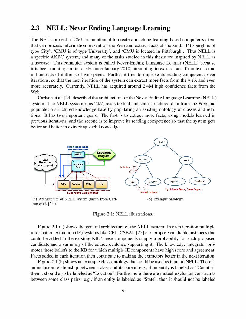
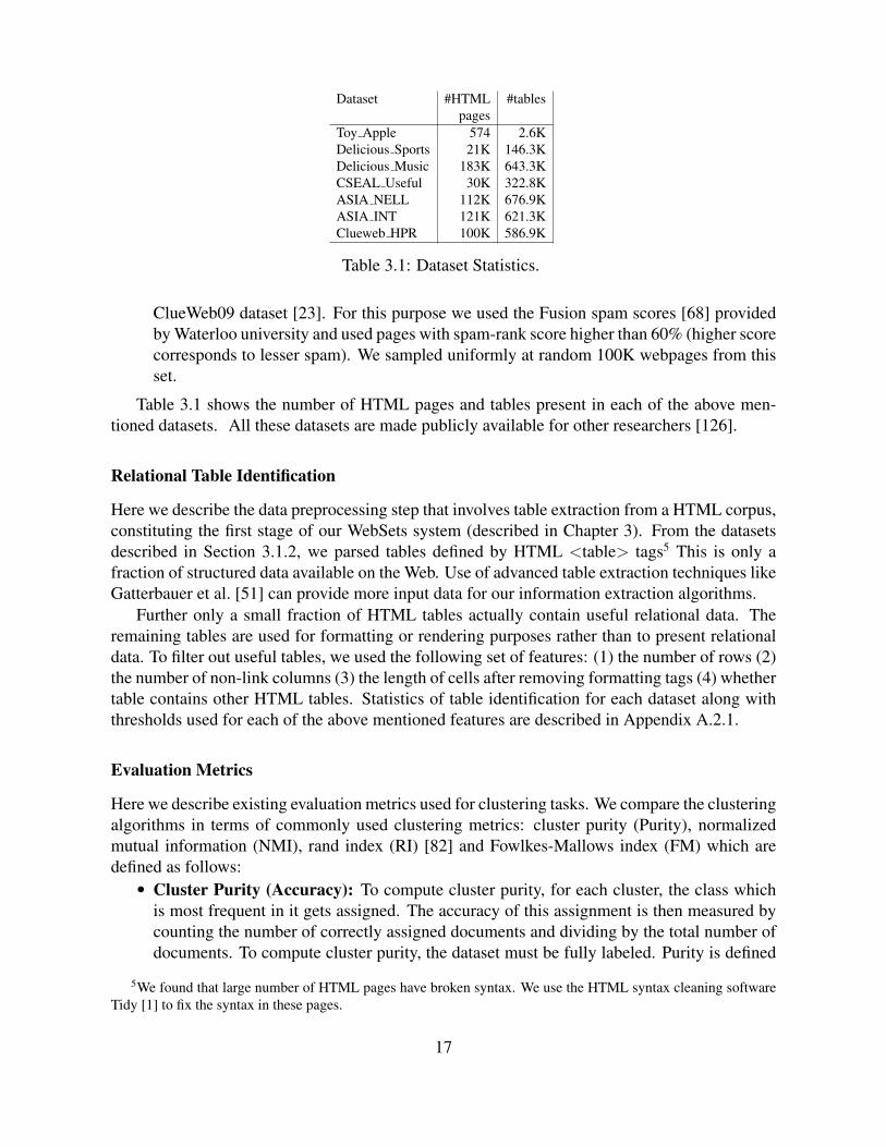
2.3 NELL: Never Ending Language LearningThe NELL project at CMU is an attempt to create a machine learning based computer systemthat can process information present on the Web and extract facts of the kind: ‘Pittsburgh is oftype City’, ‘CMU is of type University’, and ‘CMU is located in Pittsburgh’. Thus NELL isa specific AKBC system, and many of the tasks studied in this thesis are inspired by NELL asa usecase. This computer system is called Never-Ending Language Learner (NELL) becauseit is been running continuously since January 2010, attempting to extract facts from text foundin hundreds of millions of web pages. Further it tries to improve its reading competence overiterations, so that the next iteration of the system can extract more facts from the web, and evenmore accurately. Currently, NELL has acquired around 2.4M high confidence facts from theWeb.

Carlson et al. [24] described the architecture for the Never Ending Language Learning (NELL)system. The NELL system runs 24/7, reads textual and semi-structured data from the Web andpopulates a structured knowledge base by populating an existing ontology of classes and rela-tions. It has two important goals. The first is to extract more facts, using models learned inprevious iterations, and the second is to improve its reading competence so that the system getsbetter and better in extracting such knowledge.

(a) Architecture of NELL system (taken from Carl-son et al. [24]).

(b) Example ontology.

Figure 2.1: NELL illustrations.

Figure 2.1 (a) shows the general architecture of the NELL system. In each iteration multipleinformation extraction (IE) systems like CPL, CSEAL [25] etc. propose candidate instances thatcould be added to the existing KB. These components supply a probability for each proposedcandidate and a summary of the source evidence supporting it. The knowledge integrator pro-motes those beliefs to the KB for which multiple IE components have high score and agreement.Facts added in each iteration then contribute to making the extractors better in the next iteration.

Figure 2.1 (b) shows an example class ontology that could be used as input to NELL. There isan inclusion relationship between a class and its parent: e.g., if an entity is labeled as “Country”then it should also be labeled as “Location”. Furthermore there are mutual-exclusion constraintsbetween some class pairs: e.g., if an entity is labeled as “State”, then it should not be labeled

9

as “Country”. There are seed examples for each of the concepts in the ontology: e.g., Spinach,Potato etc. are seed examples of the “Vegetable” class. Thus the NELL system takes as input anontology of concepts that includes inclusion and mutual exclusion class constraints, along withseed examples, iteratively learns models for concepts, and populates them with new instances,without violating the class constraints.

10

Chapter 3

Case Study: Table Driven InformationExtraction

In this chapter, we describe an open-domain information extraction method for extracting concept-instance pairs from an HTML corpus. This work is published in the proceedings of WSDM 2012[126]. This chapter also illustrates the motivations behind the three semi-supervised learningscenarios that are focus of this thesis.

The most effective earlier approaches to the problem of concept-instance pair extraction (e.g.,Pantel et al. [100], Van Durme and Pasca [132]) rely on combining clusters of distributionallysimilar terms and concept-instance pairs obtained with Hearst patterns1[61]. In contrast, ourmethod relies on a novel approach for clustering terms found in HTML tables, and then assigningconcept names to these clusters using Hearst patterns. Note here that the names of concepts arenot coming from a fixed ontology. The method can be efficiently applied to a large corpus,and experimental results on several datasets showed that our method can accurately extract largenumbers of concept-instance pairs.

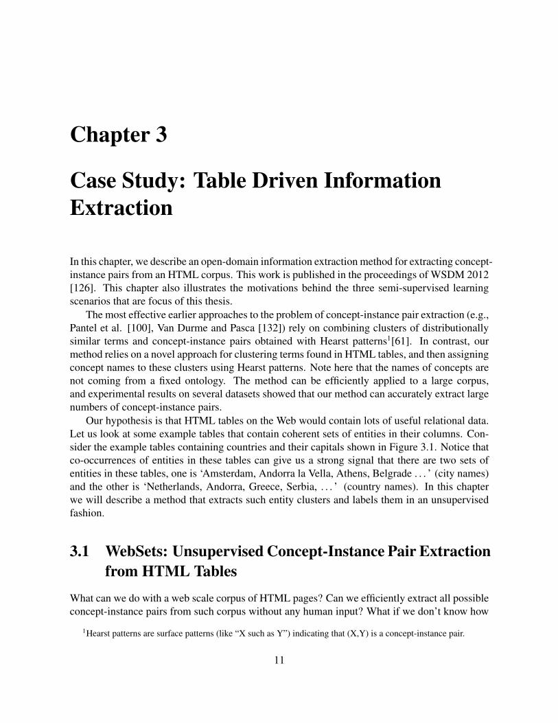
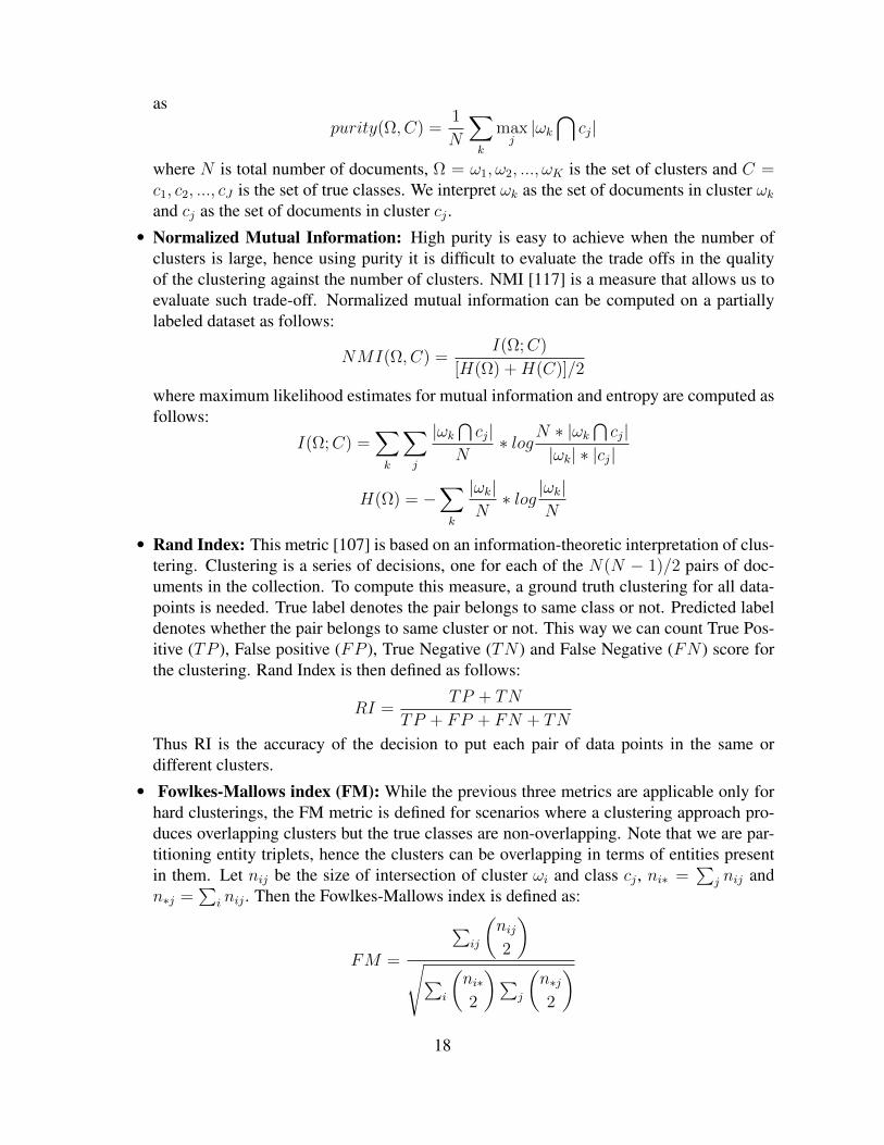
Our hypothesis is that HTML tables on the Web would contain lots of useful relational data.Let us look at some example tables that contain coherent sets of entities in their columns. Con-sider the example tables containing countries and their capitals shown in Figure 3.1. Notice thatco-occurrences of entities in these tables can give us a strong signal that there are two sets ofentities in these tables, one is ‘Amsterdam, Andorra la Vella, Athens, Belgrade . . . ’ (city names)and the other is ‘Netherlands, Andorra, Greece, Serbia, . . . ’ (country names). In this chapterwe will describe a method that extracts such entity clusters and labels them in an unsupervisedfashion.

3.1 WebSets: Unsupervised Concept-Instance Pair Extractionfrom HTML Tables

What can we do with a web scale corpus of HTML pages? Can we efficiently extract all possibleconcept-instance pairs from such corpus without any human input? What if we don’t know how

1Hearst patterns are surface patterns (like “X such as Y”) indicating that (X,Y) is a concept-instance pair.

11

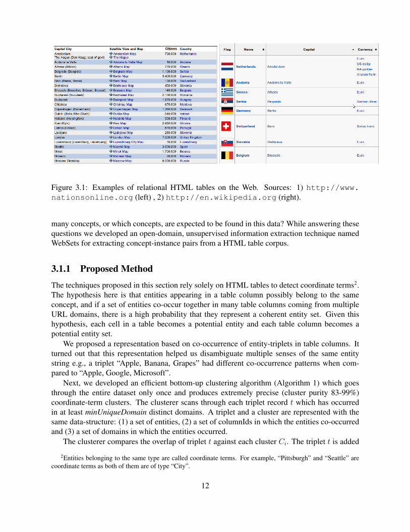
Figure 3.1: Examples of relational HTML tables on the Web. Sources: 1) http://www.nationsonline.org (left) , 2) http://en.wikipedia.org (right).

many concepts, or which concepts, are expected to be found in this data? While answering thesequestions we developed an open-domain, unsupervised information extraction technique namedWebSets for extracting concept-instance pairs from a HTML table corpus.

3.1.1 Proposed Method

The techniques proposed in this section rely solely on HTML tables to detect coordinate terms2.The hypothesis here is that entities appearing in a table column possibly belong to the sameconcept, and if a set of entities co-occur together in many table columns coming from multipleURL domains, there is a high probability that they represent a coherent entity set. Given thishypothesis, each cell in a table becomes a potential entity and each table column becomes apotential entity set.

We proposed a representation based on co-occurrence of entity-triplets in table columns. Itturned out that this representation helped us disambiguate multiple senses of the same entitystring e.g., a triplet “Apple, Banana, Grapes” had different co-occurrence patterns when com-pared to “Apple, Google, Microsoft”.

Next, we developed an efficient bottom-up clustering algorithm (Algorithm 1) which goesthrough the entire dataset only once and produces extremely precise (cluster purity 83-99%)coordinate-term clusters. The clusterer scans through each triplet record t which has occurredin at least minUniqueDomain distinct domains. A triplet and a cluster are represented with thesame data-structure: (1) a set of entities, (2) a set of columnIds in which the entities co-occurredand (3) a set of domains in which the entities occurred.

The clusterer compares the overlap of triplet t against each cluster Ci. The triplet t is added

2Entities belonging to the same type are called coordinate terms. For example, “Pittsburgh” and “Seattle” arecoordinate terms as both of them are of type “City”.

12

to the first Ci so that either of the following two cases is true:(1) at least 2 entities from t appear in cluster Ci i.e., minEntityOverlap = 2, and(2) at least 2 columnIds from t appear in cluster Ci i.e., minColumnOverlap = 2.In both these cases, intuitively there is a high probability that t belongs to the same category ascluster Ci. If no such overlap is found with existing clusters, the algorithm creates a new clusterand initializes it with the triplet t.

This clustering algorithm is order dependent, i.e., if the order in which records are processedchanges, it might return a different set of clusters. Finding the optimal ordering of triplets is ahard problem, but a reasonably good ordering can be easily generated by ordering the triplets inthe descending order of number of distinct domains. We discard triplets that appear in less thanminUniqueDomain domains.

This clustering method outperforms K-means [126] in terms of Purity, and FM index (metricsare defined in Section 3.1.2). Further, the time complexity of our clustering algorithm is onlyO(N ∗ logN) (N being total number of HTML table cells in the corpus), making it more efficientand scalable than K-means3 or agglomerative clustering4. We also presented a new method forcombining candidate concept-instance pairs and coordinate-term clusters, and used it to suggesthypernyms for entity clusters (Algorithm 2).

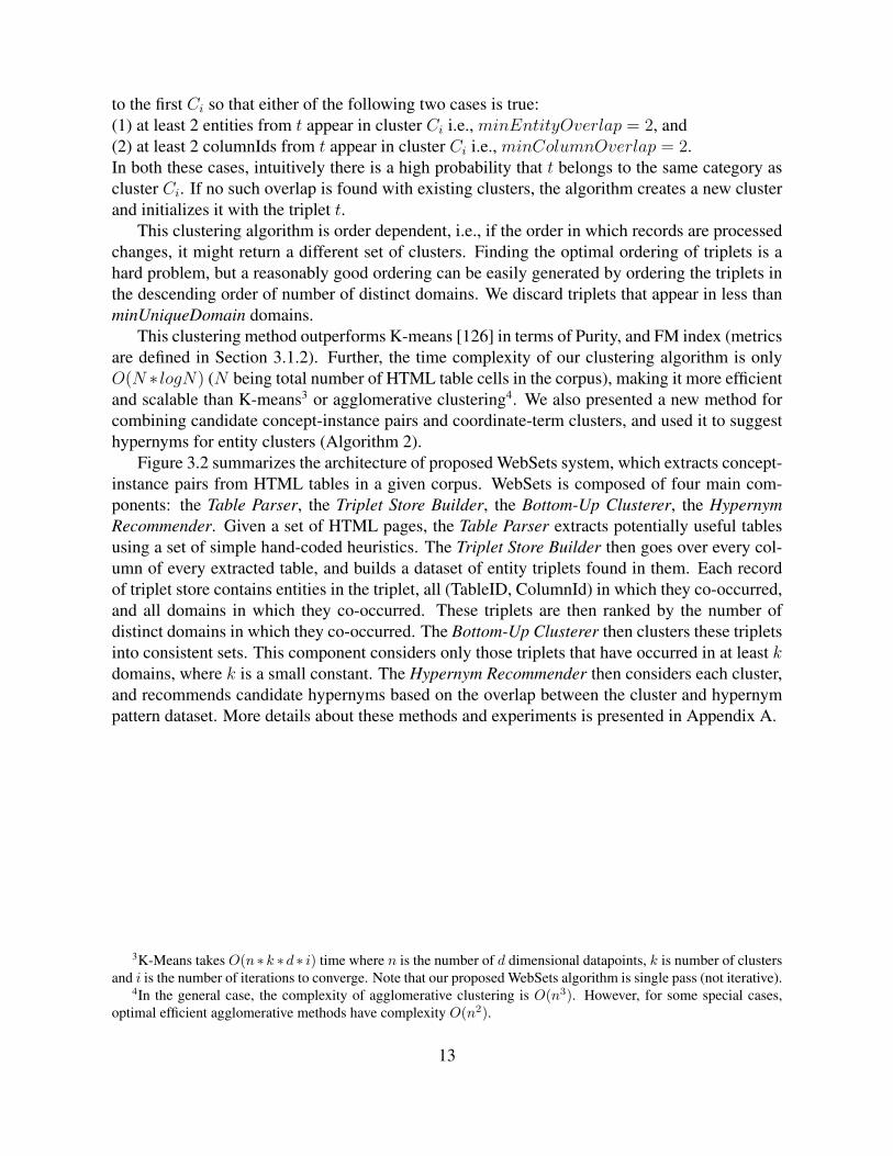
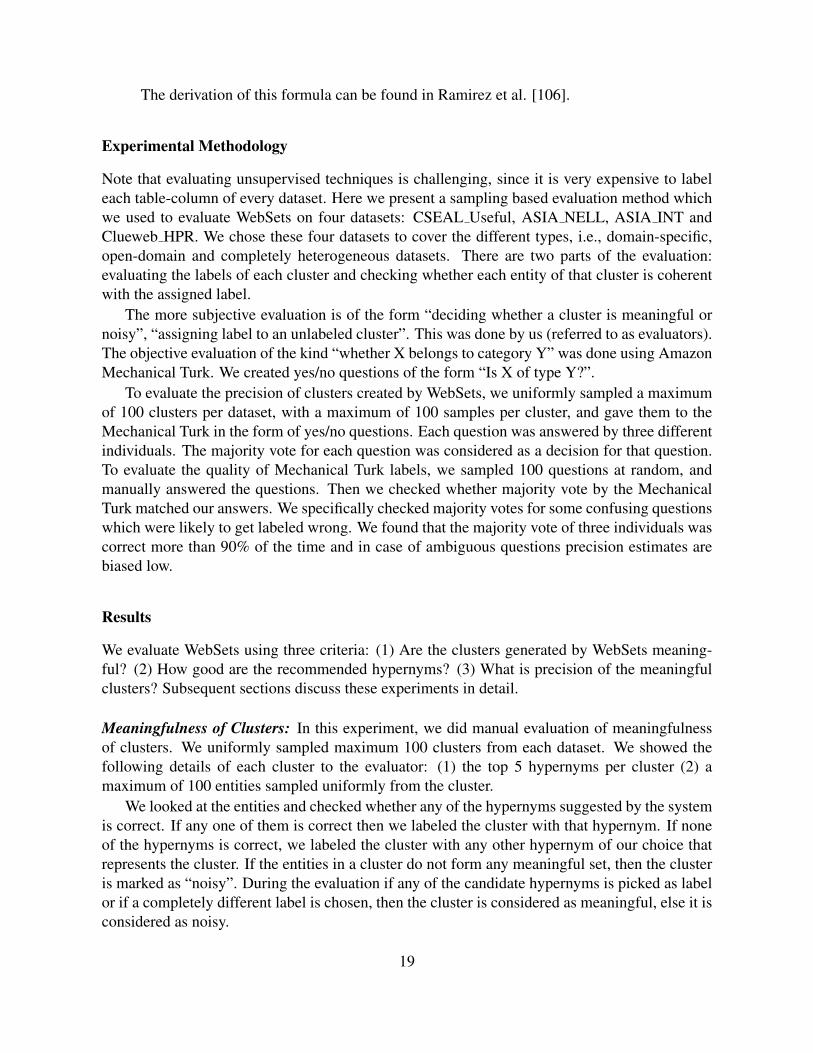
Figure 3.2 summarizes the architecture of proposed WebSets system, which extracts concept-instance pairs from HTML tables in a given corpus. WebSets is composed of four main com-ponents: the Table Parser, the Triplet Store Builder, the Bottom-Up Clusterer, the HypernymRecommender. Given a set of HTML pages, the Table Parser extracts potentially useful tablesusing a set of simple hand-coded heuristics. The Triplet Store Builder then goes over every col-umn of every extracted table, and builds a dataset of entity triplets found in them. Each recordof triplet store contains entities in the triplet, all (TableID, ColumnId) in which they co-occurred,and all domains in which they co-occurred. These triplets are then ranked by the number ofdistinct domains in which they co-occurred. The Bottom-Up Clusterer then clusters these tripletsinto consistent sets. This component considers only those triplets that have occurred in at least kdomains, where k is a small constant. The Hypernym Recommender then considers each cluster,and recommends candidate hypernyms based on the overlap between the cluster and hypernympattern dataset. More details about these methods and experiments is presented in Appendix A.

3K-Means takes O(n ∗ k ∗ d ∗ i) time where n is the number of d dimensional datapoints, k is number of clustersand i is the number of iterations to converge. Note that our proposed WebSets algorithm is single pass (not iterative).

4In the general case, the complexity of agglomerative clustering is O(n3). However, for some special cases,optimal efficient agglomerative methods have complexity O(n2).

13

Algorithm 1 Bottom-Up Clustering Algorithm.1: function Bottom-Up-Clusterer (TripletStore) :Clusters Triplet records are ordered in

descending order of number of distinct domains.2: Initialize Clusters = φ; max = 03: for (every t ∈ TripletStore : such that

|t.domains| >=minUniqueDomain) do4: assigned = false5: for every Ci ∈ Clusters do6: if |t.entities ∩ Ci.entities| >= minEntityOverlap OR |t.col ∩ Ci.col| >=

minColumnOverlap then7: Ci = Ci ∪ t8: assigned = true9: break;

10: end if11: end for12: if not assigned then13: increment max14: Create new cluster Cmax = t15: Clusters = Clusters ∪ Cmax16: end if17: end for18: end function

Algorithm 2 Hypernym Recommendation Algorithm.1: function GenerateHypernyms2: Given: c: An entity cluster generated by Algorithm 1,I: Set of all entities ,L: Set of all labels,H ⊆ L× I: Hyponym-concept dataset,

3: Returns: RLc : Ranked list of hypernyms for c.4: Algorithm:5: RLc = φ6: for every label l ∈ L do7: Hl = Set of entities which co-occurred with l in H8: Score(l) = |Hl ∩ c|9: RLc = RLc ∪ < l, Score(l) >

10: end for11: Sort RLc in descending order of Score(l)12: Output RLc13: end function

14

Figure 3.2: Architecture of the WebSets system.

15

3.1.2 Experimental Results

Here we describe the experimental results of applying WebSets techniques on various HTMLtable datasets extracted from the Web.

Datasets

To test the performance of WebSets, we created several webpage datasets that are likely to havecoherent sets of entities. An evaluation can then be done to check whether the system extractsthe expected entity sets from those datasets.

The first two datasets are created by crawling webpages that are tagged with particular topicsin the delicious.com website [139]. The next four datasets are created using the SEAL [25, 137]and ASIA [136] systems which extract information from semi-structured pages on the Web.Each of these systems takes as input a name or seed examples of a category, and finds possibleinstances of that category using set expansion techniques. The last dataset is sampled from theClueWeb09 corpus. We expect these datasets to be rich in semi-structured data.

1. Delicious Sports: This dataset is a subset of the DAI-Labor Delicious corpus [139] whichcontains all public bookmarks of about 950,000 users retrieved from ‘delicious.com’ be-tween December 2007 and April 2008. Delicious Sports is created by taking only thoseURLs which are tagged as “sports”.

2. Delicious Music: This dataset is a subset of the DAI-Labor Delicious corpus [139], cre-ated by taking only those URLs which are tagged as “music”.

3. CSEAL Useful: CSEAL is one of the methods which suggests new category and relationinstances to NELL. It mostly extracts entities out of semi-structured information on theWeb. CSEAL Useful dataset is a collection of those HTML pages from which CSEALgathered information about entities in the NELL KB.

4. Toy Apple: This is a small toy dataset created with the help of multiple SEAL queries suchthat it contains instances of word “Apple” as a fruit and “Apple” as a company. Throughthis dataset we tackle the challenge of separating multiple senses of a word. We alsostudied how different clustering algorithms and different entity representations perform onthe clustering task.

5. ASIA NELL: ASIA [136] extracts instances of a given semantic class name (e.g., ‘carmakers’ to ‘Ford, Nissan, Toyota . . . ’) in an unsupervised fashion. It extracts set instancesby utilizing Hearst patterns [61] along with the state-of-the-art set expansion techniqueimplemented in SEAL. ASIA NELL dataset is collected using hypernyms associated withentities in the NELL KB as queries for ASIA. Examples of such hypernyms are “City”,“Bird”, “Sports team” etc.

6. ASIA INT: This dataset is also collected using the ASIA system but with another set ofcategory names as input. These category names come from the intelligence domain. Ex-amples of categories in this domain are “government types”, “international organizations”,“federal agencies”, “religions” etc.

7. Clueweb HPR: This dataset is collected by randomly sampling high quality pages in the

16

Dataset #HTML #tablespages

Toy Apple 574 2.6KDelicious Sports 21K 146.3KDelicious Music 183K 643.3KCSEAL Useful 30K 322.8KASIA NELL 112K 676.9KASIA INT 121K 621.3KClueweb HPR 100K 586.9K

Table 3.1: Dataset Statistics.

ClueWeb09 dataset [23]. For this purpose we used the Fusion spam scores [68] providedby Waterloo university and used pages with spam-rank score higher than 60% (higher scorecorresponds to lesser spam). We sampled uniformly at random 100K webpages from thisset.

Table 3.1 shows the number of HTML pages and tables present in each of the above men-tioned datasets. All these datasets are made publicly available for other researchers [126].

Relational Table Identification

Here we describe the data preprocessing step that involves table extraction from a HTML corpus,constituting the first stage of our WebSets system (described in Chapter 3). From the datasetsdescribed in Section 3.1.2, we parsed tables defined by HTML <table> tags5 This is only afraction of structured data available on the Web. Use of advanced table extraction techniques likeGatterbauer et al. [51] can provide more input data for our information extraction algorithms.

Further only a small fraction of HTML tables actually contain useful relational data. Theremaining tables are used for formatting or rendering purposes rather than to present relationaldata. To filter out useful tables, we used the following set of features: (1) the number of rows (2)the number of non-link columns (3) the length of cells after removing formatting tags (4) whethertable contains other HTML tables. Statistics of table identification for each dataset along withthresholds used for each of the above mentioned features are described in Appendix A.2.1.

Evaluation Metrics

Here we describe existing evaluation metrics used for clustering tasks. We compare the clusteringalgorithms in terms of commonly used clustering metrics: cluster purity (Purity), normalizedmutual information (NMI), rand index (RI) [82] and Fowlkes-Mallows index (FM) which aredefined as follows:• Cluster Purity (Accuracy): To compute cluster purity, for each cluster, the class which

is most frequent in it gets assigned. The accuracy of this assignment is then measured bycounting the number of correctly assigned documents and dividing by the total number ofdocuments. To compute cluster purity, the dataset must be fully labeled. Purity is defined

5We found that large number of HTML pages have broken syntax. We use the HTML syntax cleaning softwareTidy [1] to fix the syntax in these pages.

17

aspurity(Ω, C) =

1

N

∑k

maxj|ωk⋂

cj|

where N is total number of documents, Ω = ω1, ω2, ..., ωK is the set of clusters and C =c1, c2, ..., cJ is the set of true classes. We interpret ωk as the set of documents in cluster ωkand cj as the set of documents in cluster cj .

• Normalized Mutual Information: High purity is easy to achieve when the number ofclusters is large, hence using purity it is difficult to evaluate the trade offs in the qualityof the clustering against the number of clusters. NMI [117] is a measure that allows us toevaluate such trade-off. Normalized mutual information can be computed on a partiallylabeled dataset as follows:

NMI(Ω, C) =I(Ω;C)

[H(Ω) +H(C)]/2

where maximum likelihood estimates for mutual information and entropy are computed asfollows:

I(Ω;C) =∑k

∑j

|ωk⋂cj|

N∗ logN ∗ |ωk

⋂cj|

|ωk| ∗ |cj|

H(Ω) = −∑k

|ωk|N∗ log |ωk|

N

• Rand Index: This metric [107] is based on an information-theoretic interpretation of clus-tering. Clustering is a series of decisions, one for each of the N(N − 1)/2 pairs of doc-uments in the collection. To compute this measure, a ground truth clustering for all data-points is needed. True label denotes the pair belongs to same class or not. Predicted labeldenotes whether the pair belongs to same cluster or not. This way we can count True Pos-itive (TP ), False positive (FP ), True Negative (TN ) and False Negative (FN ) score forthe clustering. Rand Index is then defined as follows:

RI =TP + TN

TP + FP + FN + TN

Thus RI is the accuracy of the decision to put each pair of data points in the same ordifferent clusters.

• Fowlkes-Mallows index (FM): While the previous three metrics are applicable only forhard clusterings, the FM metric is defined for scenarios where a clustering approach pro-duces overlapping clusters but the true classes are non-overlapping. Note that we are par-titioning entity triplets, hence the clusters can be overlapping in terms of entities presentin them. Let nij be the size of intersection of cluster ωi and class cj , ni∗ =

∑j nij and

n∗j =∑

i nij . Then the Fowlkes-Mallows index is defined as:

FM =

∑ij

(nij2

)√∑

i

(ni∗2

)∑j

(n∗j2

)18

The derivation of this formula can be found in Ramirez et al. [106].

Experimental Methodology

Note that evaluating unsupervised techniques is challenging, since it is very expensive to labeleach table-column of every dataset. Here we present a sampling based evaluation method whichwe used to evaluate WebSets on four datasets: CSEAL Useful, ASIA NELL, ASIA INT andClueweb HPR. We chose these four datasets to cover the different types, i.e., domain-specific,open-domain and completely heterogeneous datasets. There are two parts of the evaluation:evaluating the labels of each cluster and checking whether each entity of that cluster is coherentwith the assigned label.

The more subjective evaluation is of the form “deciding whether a cluster is meaningful ornoisy”, “assigning label to an unlabeled cluster”. This was done by us (referred to as evaluators).The objective evaluation of the kind “whether X belongs to category Y” was done using AmazonMechanical Turk. We created yes/no questions of the form “Is X of type Y?”.

To evaluate the precision of clusters created by WebSets, we uniformly sampled a maximumof 100 clusters per dataset, with a maximum of 100 samples per cluster, and gave them to theMechanical Turk in the form of yes/no questions. Each question was answered by three differentindividuals. The majority vote for each question was considered as a decision for that question.To evaluate the quality of Mechanical Turk labels, we sampled 100 questions at random, andmanually answered the questions. Then we checked whether majority vote by the MechanicalTurk matched our answers. We specifically checked majority votes for some confusing questionswhich were likely to get labeled wrong. We found that the majority vote of three individuals wascorrect more than 90% of the time and in case of ambiguous questions precision estimates arebiased low.

Results

We evaluate WebSets using three criteria: (1) Are the clusters generated by WebSets meaning-ful? (2) How good are the recommended hypernyms? (3) What is precision of the meaningfulclusters? Subsequent sections discuss these experiments in detail.

Meaningfulness of Clusters: In this experiment, we did manual evaluation of meaningfulnessof clusters. We uniformly sampled maximum 100 clusters from each dataset. We showed thefollowing details of each cluster to the evaluator: (1) the top 5 hypernyms per cluster (2) amaximum of 100 entities sampled uniformly from the cluster.

We looked at the entities and checked whether any of the hypernyms suggested by the systemis correct. If any one of them is correct then we labeled the cluster with that hypernym. If noneof the hypernyms is correct, we labeled the cluster with any other hypernym of our choice thatrepresents the cluster. If the entities in a cluster do not form any meaningful set, then the clusteris marked as “noisy”. During the evaluation if any of the candidate hypernyms is picked as labelor if a completely different label is chosen, then the cluster is considered as meaningful, else it isconsidered as noisy.

19

#Triplets #Clusters #clusters with Hypernyms % meaningfulCSEAL Useful 165.2K 1090 312 69.0%ASIA NELL 11.4K 448 266 73.0%ASIA INT 15.1K 395 218 63.0%Clueweb HPR 561.0 47 34 70.5%

Table 3.2: Meaningfulness of generated clusters.

#Clusters Evaluated #Meaningful Clusters #Hypernyms correct MRR (meaningful)CSEAL Useful 100 69 57 0.56ASIA NELL 100 73 66 0.59ASIA INT 100 63 50 0.58Clueweb HPR 34 24 20 0.56

Table 3.3: Evaluation of Hypernym Recommender.

Table 3.2 shows that 63-73% of the clusters were labeled as meaningful. Note that number oftriplets used by the clustering algorithm (Table 3.2) is different from total number of triplets inthe triplet store (Table A.6), because only those triplets that occur in at least minUniqueDomain(set to 2 for all experiments) distinct domains are clustered.

Performance of Hypernym Recommendation: In this experiment, we evaluate the performanceof the hypernym recommendation using the following criterion:(1) What fraction of the total clusters were assigned some hypernym?: This can be directly com-puted by looking at the outputs generated by hypernym recommendation.(2) For what fraction of clusters did the evaluator chose the label from the recommended hyper-nyms?: This can be computed by checking whether each of the manually assigned labels wasone of the recommended labels.(3) What is Mean Reciprocal Rank (MRR) of the hypernym ranking?: The evaluator gets to seeranked list of top 5 labels suggested by the hypernym recommender. We compute MRR based onrank of the label selected by the evaluator. While calculating MRR, we consider all meaningfulclusters (including the ones for which label does not come from the recommended hypernyms).

Table 3.3 shows the results of this evaluation. Out of the random sample of clusters evaluated,hypernym recommendation could label 50-60% of them correctly. The MRR of labels is 0.56-0.59 for all the datasets.

Next we compare our hypernym recommendation technique with Van Durme and Pasca tech-nique [132]. Our method is different from Van Durme and Pasca Method (DPM) in the sense that,they output a concept-instance pair only when it appears in a set of candidate concept-instancepairs, i.e., it exists in Hyponym-concept dataset. In our method, based on overlap of coordinateterm cluster with the Hyponym Concept dataset, we extend the labels to the whole cluster. An-other difference is the coordinate term clusters we are dealing with. DPM assumes term clustersare semantic partitions of terms present in the text corpus. The clusters generated by WebSetsare clusters of table columns. There is higher possibility of having multiple small size clusterswhich all belong to same semantic class, but were not merged due to our single pass bottom-upclusterer. Hence the same method may not work equally well on these clusters.

20

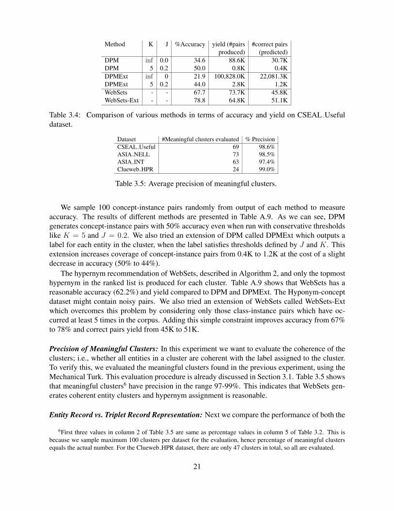
Method K J %Accuracy yield (#pairs #correct pairsproduced) (predicted)

DPM inf 0.0 34.6 88.6K 30.7KDPM 5 0.2 50.0 0.8K 0.4KDPMExt inf 0 21.9 100,828.0K 22,081.3KDPMExt 5 0.2 44.0 2.8K 1.2KWebSets - - 67.7 73.7K 45.8KWebSets-Ext - - 78.8 64.8K 51.1K

Table 3.4: Comparison of various methods in terms of accuracy and yield on CSEAL Usefuldataset.

Dataset #Meaningful clusters evaluated % PrecisionCSEAL Useful 69 98.6%ASIA NELL 73 98.5%ASIA INT 63 97.4%Clueweb HPR 24 99.0%

Table 3.5: Average precision of meaningful clusters.

We sample 100 concept-instance pairs randomly from output of each method to measureaccuracy. The results of different methods are presented in Table A.9. As we can see, DPMgenerates concept-instance pairs with 50% accuracy even when run with conservative thresholdslike K = 5 and J = 0.2. We also tried an extension of DPM called DPMExt which outputs alabel for each entity in the cluster, when the label satisfies thresholds defined by J and K. Thisextension increases coverage of concept-instance pairs from 0.4K to 1.2K at the cost of a slightdecrease in accuracy (50% to 44%).

The hypernym recommendation of WebSets, described in Algorithm 2, and only the topmosthypernym in the ranked list is produced for each cluster. Table A.9 shows that WebSets has areasonable accuracy (62.2%) and yield compared to DPM and DPMExt. The Hyponym-conceptdataset might contain noisy pairs. We also tried an extension of WebSets called WebSets-Extwhich overcomes this problem by considering only those class-instance pairs which have oc-curred at least 5 times in the corpus. Adding this simple constraint improves accuracy from 67%to 78% and correct pairs yield from 45K to 51K.

Precision of Meaningful Clusters: In this experiment we want to evaluate the coherence of theclusters; i.e., whether all entities in a cluster are coherent with the label assigned to the cluster.To verify this, we evaluated the meaningful clusters found in the previous experiment, using theMechanical Turk. This evaluation procedure is already discussed in Section 3.1. Table 3.5 showsthat meaningful clusters6 have precision in the range 97-99%. This indicates that WebSets gen-erates coherent entity clusters and hypernym assignment is reasonable.

Entity Record vs. Triplet Record Representation: Next we compare the performance of both the

6First three values in column 2 of Table 3.5 are same as percentage values in column 5 of Table 3.2. This isbecause we sample maximum 100 clusters per dataset for the evaluation, hence percentage of meaningful clustersequals the actual number. For the Clueweb HPR dataset, there are only 47 clusters in total, so all are evaluated.

21

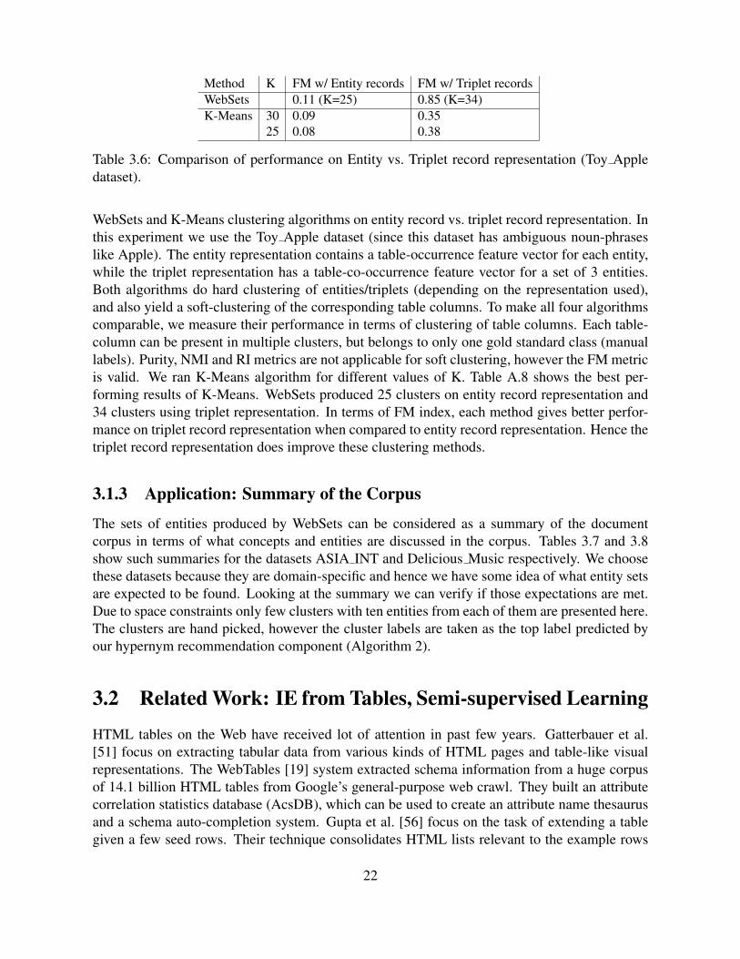
Method K FM w/ Entity records FM w/ Triplet recordsWebSets 0.11 (K=25) 0.85 (K=34)K-Means 30 0.09 0.35

25 0.08 0.38

Table 3.6: Comparison of performance on Entity vs. Triplet record representation (Toy Appledataset).

WebSets and K-Means clustering algorithms on entity record vs. triplet record representation. Inthis experiment we use the Toy Apple dataset (since this dataset has ambiguous noun-phraseslike Apple). The entity representation contains a table-occurrence feature vector for each entity,while the triplet representation has a table-co-occurrence feature vector for a set of 3 entities.Both algorithms do hard clustering of entities/triplets (depending on the representation used),and also yield a soft-clustering of the corresponding table columns. To make all four algorithmscomparable, we measure their performance in terms of clustering of table columns. Each table-column can be present in multiple clusters, but belongs to only one gold standard class (manuallabels). Purity, NMI and RI metrics are not applicable for soft clustering, however the FM metricis valid. We ran K-Means algorithm for different values of K. Table A.8 shows the best per-forming results of K-Means. WebSets produced 25 clusters on entity record representation and34 clusters using triplet representation. In terms of FM index, each method gives better perfor-mance on triplet record representation when compared to entity record representation. Hence thetriplet record representation does improve these clustering methods.

3.1.3 Application: Summary of the Corpus

The sets of entities produced by WebSets can be considered as a summary of the documentcorpus in terms of what concepts and entities are discussed in the corpus. Tables 3.7 and 3.8show such summaries for the datasets ASIA INT and Delicious Music respectively. We choosethese datasets because they are domain-specific and hence we have some idea of what entity setsare expected to be found. Looking at the summary we can verify if those expectations are met.Due to space constraints only few clusters with ten entities from each of them are presented here.The clusters are hand picked, however the cluster labels are taken as the top label predicted byour hypernym recommendation component (Algorithm 2).

3.2 Related Work: IE from Tables, Semi-supervised Learning

HTML tables on the Web have received lot of attention in past few years. Gatterbauer et al.[51] focus on extracting tabular data from various kinds of HTML pages and table-like visualrepresentations. The WebTables [19] system extracted schema information from a huge corpusof 14.1 billion HTML tables from Google’s general-purpose web crawl. They built an attributecorrelation statistics database (AcsDB), which can be used to create an attribute name thesaurusand a schema auto-completion system. Gupta et al. [56] focus on the task of extending a tablegiven a few seed rows. Their technique consolidates HTML lists relevant to the example rows

22

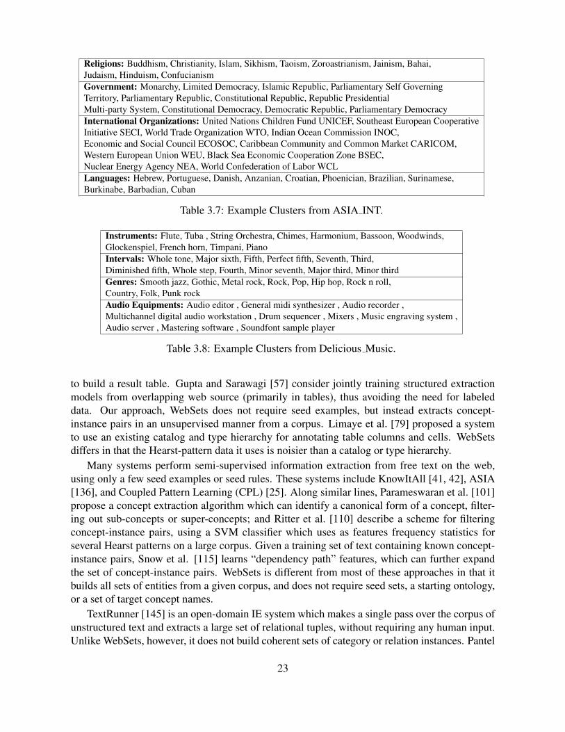
Religions: Buddhism, Christianity, Islam, Sikhism, Taoism, Zoroastrianism, Jainism, Bahai,Judaism, Hinduism, ConfucianismGovernment: Monarchy, Limited Democracy, Islamic Republic, Parliamentary Self GoverningTerritory, Parliamentary Republic, Constitutional Republic, Republic PresidentialMulti-party System, Constitutional Democracy, Democratic Republic, Parliamentary DemocracyInternational Organizations: United Nations Children Fund UNICEF, Southeast European CooperativeInitiative SECI, World Trade Organization WTO, Indian Ocean Commission INOC,Economic and Social Council ECOSOC, Caribbean Community and Common Market CARICOM,Western European Union WEU, Black Sea Economic Cooperation Zone BSEC,Nuclear Energy Agency NEA, World Confederation of Labor WCLLanguages: Hebrew, Portuguese, Danish, Anzanian, Croatian, Phoenician, Brazilian, Surinamese,Burkinabe, Barbadian, Cuban

Table 3.7: Example Clusters from ASIA INT.

Instruments: Flute, Tuba , String Orchestra, Chimes, Harmonium, Bassoon, Woodwinds,Glockenspiel, French horn, Timpani, PianoIntervals: Whole tone, Major sixth, Fifth, Perfect fifth, Seventh, Third,Diminished fifth, Whole step, Fourth, Minor seventh, Major third, Minor thirdGenres: Smooth jazz, Gothic, Metal rock, Rock, Pop, Hip hop, Rock n roll,Country, Folk, Punk rockAudio Equipments: Audio editor , General midi synthesizer , Audio recorder ,Multichannel digital audio workstation , Drum sequencer , Mixers , Music engraving system ,Audio server , Mastering software , Soundfont sample player

Table 3.8: Example Clusters from Delicious Music.

to build a result table. Gupta and Sarawagi [57] consider jointly training structured extractionmodels from overlapping web source (primarily in tables), thus avoiding the need for labeleddata. Our approach, WebSets does not require seed examples, but instead extracts concept-instance pairs in an unsupervised manner from a corpus. Limaye et al. [79] proposed a systemto use an existing catalog and type hierarchy for annotating table columns and cells. WebSetsdiffers in that the Hearst-pattern data it uses is noisier than a catalog or type hierarchy.

Many systems perform semi-supervised information extraction from free text on the web,using only a few seed examples or seed rules. These systems include KnowItAll [41, 42], ASIA[136], and Coupled Pattern Learning (CPL) [25]. Along similar lines, Parameswaran et al. [101]propose a concept extraction algorithm which can identify a canonical form of a concept, filter-ing out sub-concepts or super-concepts; and Ritter et al. [110] describe a scheme for filteringconcept-instance pairs, using a SVM classifier which uses as features frequency statistics forseveral Hearst patterns on a large corpus. Given a training set of text containing known concept-instance pairs, Snow et al. [115] learns “dependency path” features, which can further expandthe set of concept-instance pairs. WebSets is different from most of these approaches in that itbuilds all sets of entities from a given corpus, and does not require seed sets, a starting ontology,or a set of target concept names.

TextRunner [145] is an open-domain IE system which makes a single pass over the corpus ofunstructured text and extracts a large set of relational tuples, without requiring any human input.Unlike WebSets, however, it does not build coherent sets of category or relation instances. Pantel

23

and Ravichandran [100] proposes a method to automatically label distributional term clustersusing Hearst-like patterns, and Van Durme and Pasca [132] proposed an alternative approachmethod to extract labeled classes of instances from unstructured text. These approaches useonly unstructured text to find coordinate terms and assigning hypernyms, whereas WebSets usesHTML tables. As we show in the experimental results, WebSets uses a novel method for combin-ing coordinate-term clusters and hypernyms data that quantitatively improves over Van Durmeand Pasca’s method for combining coordinate-term clusters and hypernym data.

There also exist some systems that use both free-text and tabular information. Talukdar et al.[121] proposed a graph random walk based semi-supervised label propagation technique for opendomain class instance extractions, which extends the system of Van Durme and Pasca by usingtable data (from WebTables) as well as free-text distributional clusters. However, unlike Taluk-dar et al.’s system, WebSets does not require distributional clusters. Coupled SEAL (CSEAL)[25] use of mutual exclusion, containment and type checking relationships to extend SEAL, andCPL [25] and CSEAL are the two components of NELL [91], a multi-strategy semi-supervisedlearning system. However, unlike NELL, WebSets does not require seed instances or an ontol-ogy as input. Shinzato and Torisawa [113] showed that coordinate terms can be extracted fromitemizations in structured web documents. Their method finds concept-instance pairs pertainingto a single query list, and finds candidate hypernyms by querying the web on-the-fly to collectdocuments. In contrast, WebSets processes all lists in a corpora simultaneously, and makes noweb queries.

In the recent years there has been more work in the area of information extraction from semi-structured data. Balasubramanyan et al. [6] used the HTML tables data extracted by WebSetsas a multi-view dataset to learn a semi-supervised mixed membership model that can make useof feature and document labels. Adelfio and Samet [3] developed a method to extract schemainformation from tables found on the webpages and in spreadsheets. They used conditionalrandom fields to determine schema including row groupings. Instead of HTML table structure,some recent techniques use DOM trees to extract information from structured webpages. Insa etal. [63] used DOM trees to analyze the hierarchical relationship between the webpage elementalong with the distribution of textual information to do content extraction. Castillo et al. [27]worked on a novel online technique that can extract information from a set of interconnectedwebpages based on DOM distances.

24

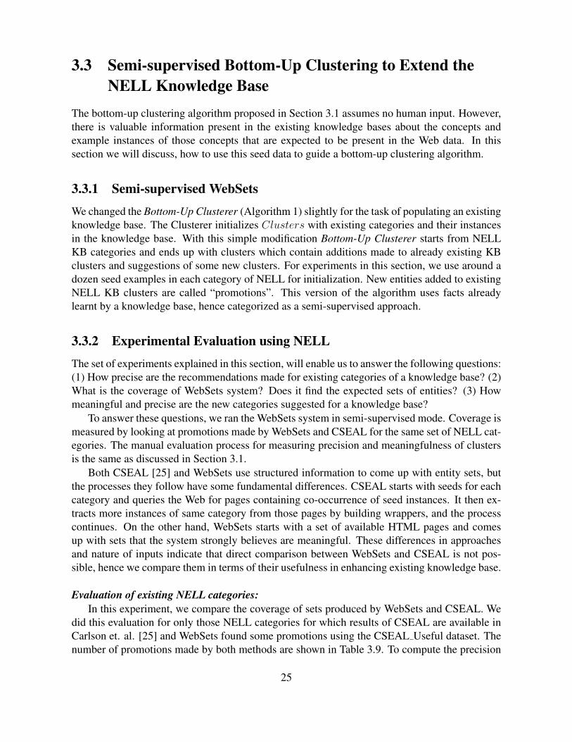
3.3 Semi-supervised Bottom-Up Clustering to Extend theNELL Knowledge Base

The bottom-up clustering algorithm proposed in Section 3.1 assumes no human input. However,there is valuable information present in the existing knowledge bases about the concepts andexample instances of those concepts that are expected to be present in the Web data. In thissection we will discuss, how to use this seed data to guide a bottom-up clustering algorithm.

3.3.1 Semi-supervised WebSets

We changed the Bottom-Up Clusterer (Algorithm 1) slightly for the task of populating an existingknowledge base. The Clusterer initializes Clusters with existing categories and their instancesin the knowledge base. With this simple modification Bottom-Up Clusterer starts from NELLKB categories and ends up with clusters which contain additions made to already existing KBclusters and suggestions of some new clusters. For experiments in this section, we use around adozen seed examples in each category of NELL for initialization. New entities added to existingNELL KB clusters are called “promotions”. This version of the algorithm uses facts alreadylearnt by a knowledge base, hence categorized as a semi-supervised approach.

3.3.2 Experimental Evaluation using NELL

The set of experiments explained in this section, will enable us to answer the following questions:(1) How precise are the recommendations made for existing categories of a knowledge base? (2)What is the coverage of WebSets system? Does it find the expected sets of entities? (3) Howmeaningful and precise are the new categories suggested for a knowledge base?

To answer these questions, we ran the WebSets system in semi-supervised mode. Coverage ismeasured by looking at promotions made by WebSets and CSEAL for the same set of NELL cat-egories. The manual evaluation process for measuring precision and meaningfulness of clustersis the same as discussed in Section 3.1.

Both CSEAL [25] and WebSets use structured information to come up with entity sets, butthe processes they follow have some fundamental differences. CSEAL starts with seeds for eachcategory and queries the Web for pages containing co-occurrence of seed instances. It then ex-tracts more instances of same category from those pages by building wrappers, and the processcontinues. On the other hand, WebSets starts with a set of available HTML pages and comesup with sets that the system strongly believes are meaningful. These differences in approachesand nature of inputs indicate that direct comparison between WebSets and CSEAL is not pos-sible, hence we compare them in terms of their usefulness in enhancing existing knowledge base.

Evaluation of existing NELL categories:In this experiment, we compare the coverage of sets produced by WebSets and CSEAL. We

did this evaluation for only those NELL categories for which results of CSEAL are available inCarlson et. al. [25] and WebSets found some promotions using the CSEAL Useful dataset. Thenumber of promotions made by both methods are shown in Table 3.9. To compute the precision

25

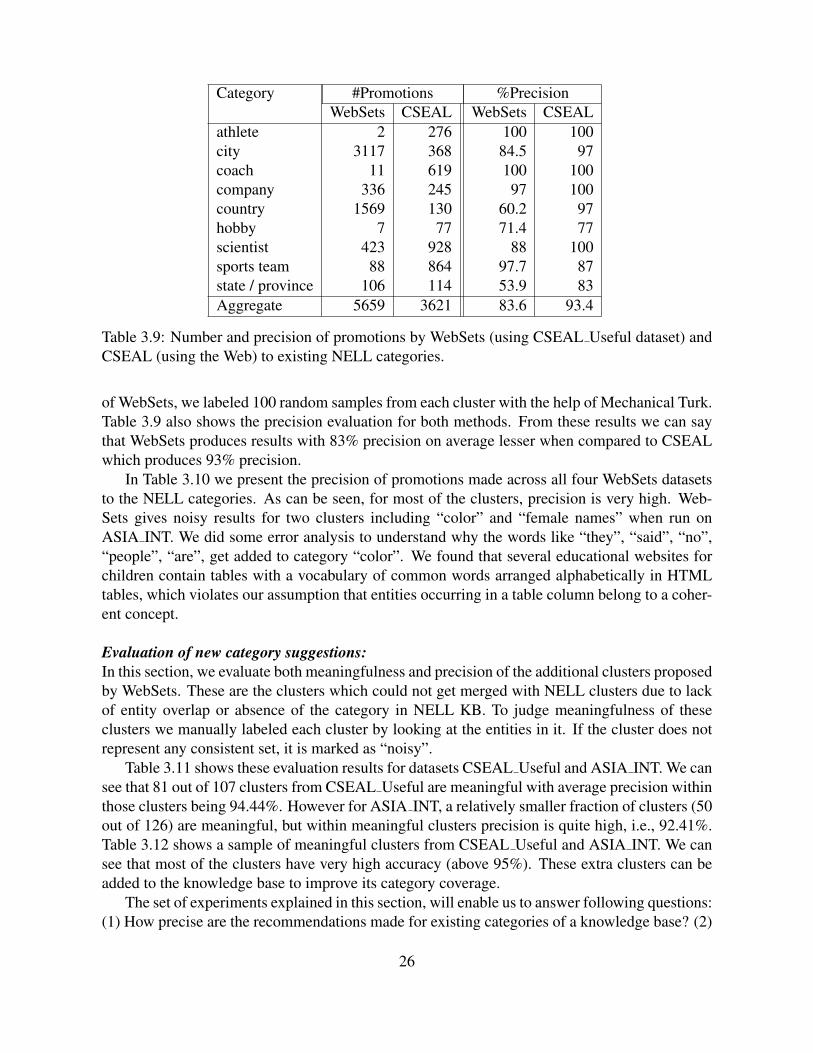
Category #Promotions %PrecisionWebSets CSEAL WebSets CSEAL

athlete 2 276 100 100city 3117 368 84.5 97coach 11 619 100 100company 336 245 97 100country 1569 130 60.2 97hobby 7 77 71.4 77scientist 423 928 88 100sports team 88 864 97.7 87state / province 106 114 53.9 83Aggregate 5659 3621 83.6 93.4

Table 3.9: Number and precision of promotions by WebSets (using CSEAL Useful dataset) andCSEAL (using the Web) to existing NELL categories.

of WebSets, we labeled 100 random samples from each cluster with the help of Mechanical Turk.Table 3.9 also shows the precision evaluation for both methods. From these results we can saythat WebSets produces results with 83% precision on average lesser when compared to CSEALwhich produces 93% precision.

In Table 3.10 we present the precision of promotions made across all four WebSets datasetsto the NELL categories. As can be seen, for most of the clusters, precision is very high. Web-Sets gives noisy results for two clusters including “color” and “female names” when run onASIA INT. We did some error analysis to understand why the words like “they”, “said”, “no”,“people”, “are”, get added to category “color”. We found that several educational websites forchildren contain tables with a vocabulary of common words arranged alphabetically in HTMLtables, which violates our assumption that entities occurring in a table column belong to a coher-ent concept.

Evaluation of new category suggestions:In this section, we evaluate both meaningfulness and precision of the additional clusters proposedby WebSets. These are the clusters which could not get merged with NELL clusters due to lackof entity overlap or absence of the category in NELL KB. To judge meaningfulness of theseclusters we manually labeled each cluster by looking at the entities in it. If the cluster does notrepresent any consistent set, it is marked as “noisy”.

Table 3.11 shows these evaluation results for datasets CSEAL Useful and ASIA INT. We cansee that 81 out of 107 clusters from CSEAL Useful are meaningful with average precision withinthose clusters being 94.44%. However for ASIA INT, a relatively smaller fraction of clusters (50out of 126) are meaningful, but within meaningful clusters precision is quite high, i.e., 92.41%.Table 3.12 shows a sample of meaningful clusters from CSEAL Useful and ASIA INT. We cansee that most of the clusters have very high accuracy (above 95%). These extra clusters can beadded to the knowledge base to improve its category coverage.

The set of experiments explained in this section, will enable us to answer following questions:(1) How precise are the recommendations made for existing categories of a knowledge base? (2)

26

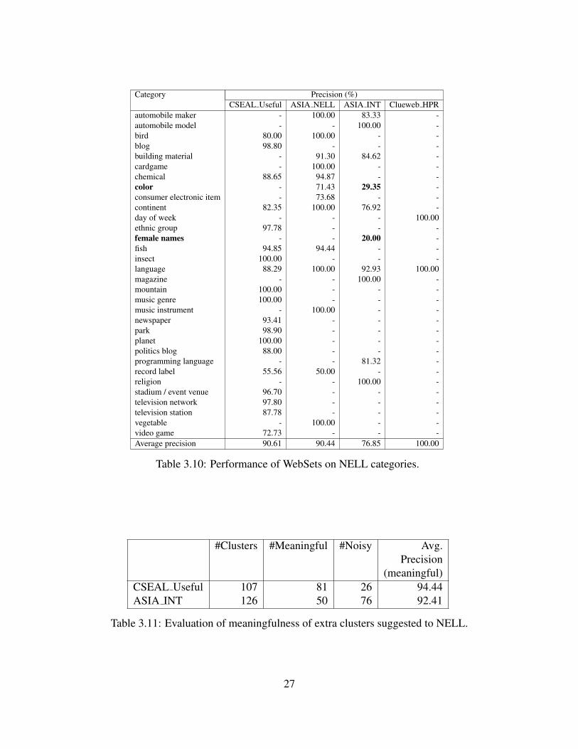
Category Precision (%)CSEAL Useful ASIA NELL ASIA INT Clueweb HPR

automobile maker - 100.00 83.33 -automobile model - - 100.00 -bird 80.00 100.00 - -blog 98.80 - - -building material - 91.30 84.62 -cardgame - 100.00 - -chemical 88.65 94.87 - -color - 71.43 29.35 -consumer electronic item - 73.68 - -continent 82.35 100.00 76.92 -day of week - - - 100.00ethnic group 97.78 - - -female names - - 20.00 -fish 94.85 94.44 - -insect 100.00 - - -language 88.29 100.00 92.93 100.00magazine - - 100.00 -mountain 100.00 - - -music genre 100.00 - - -music instrument - 100.00 - -newspaper 93.41 - - -park 98.90 - - -planet 100.00 - - -politics blog 88.00 - - -programming language - - 81.32 -record label 55.56 50.00 - -religion - - 100.00 -stadium / event venue 96.70 - - -television network 97.80 - - -television station 87.78 - - -vegetable - 100.00 - -video game 72.73 - - -Average precision 90.61 90.44 76.85 100.00

Table 3.10: Performance of WebSets on NELL categories.

#Clusters #Meaningful #Noisy Avg.Precision

(meaningful)CSEAL Useful 107 81 26 94.44ASIA INT 126 50 76 92.41

Table 3.11: Evaluation of meaningfulness of extra clusters suggested to NELL.

27

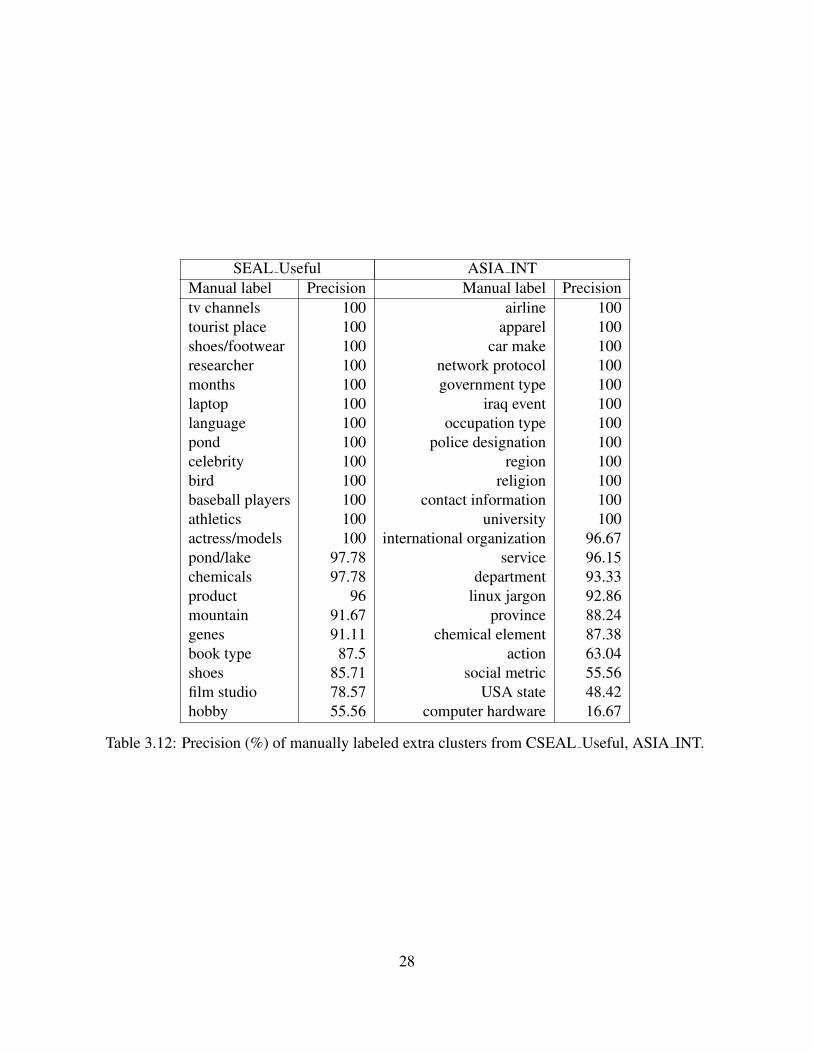
SEAL Useful ASIA INTManual label Precision Manual label Precisiontv channels 100 airline 100tourist place 100 apparel 100shoes/footwear 100 car make 100researcher 100 network protocol 100months 100 government type 100laptop 100 iraq event 100language 100 occupation type 100pond 100 police designation 100celebrity 100 region 100bird 100 religion 100baseball players 100 contact information 100athletics 100 university 100actress/models 100 international organization 96.67pond/lake 97.78 service 96.15chemicals 97.78 department 93.33product 96 linux jargon 92.86mountain 91.67 province 88.24genes 91.11 chemical element 87.38book type 87.5 action 63.04shoes 85.71 social metric 55.56film studio 78.57 USA state 48.42hobby 55.56 computer hardware 16.67

Table 3.12: Precision (%) of manually labeled extra clusters from CSEAL Useful, ASIA INT.

28

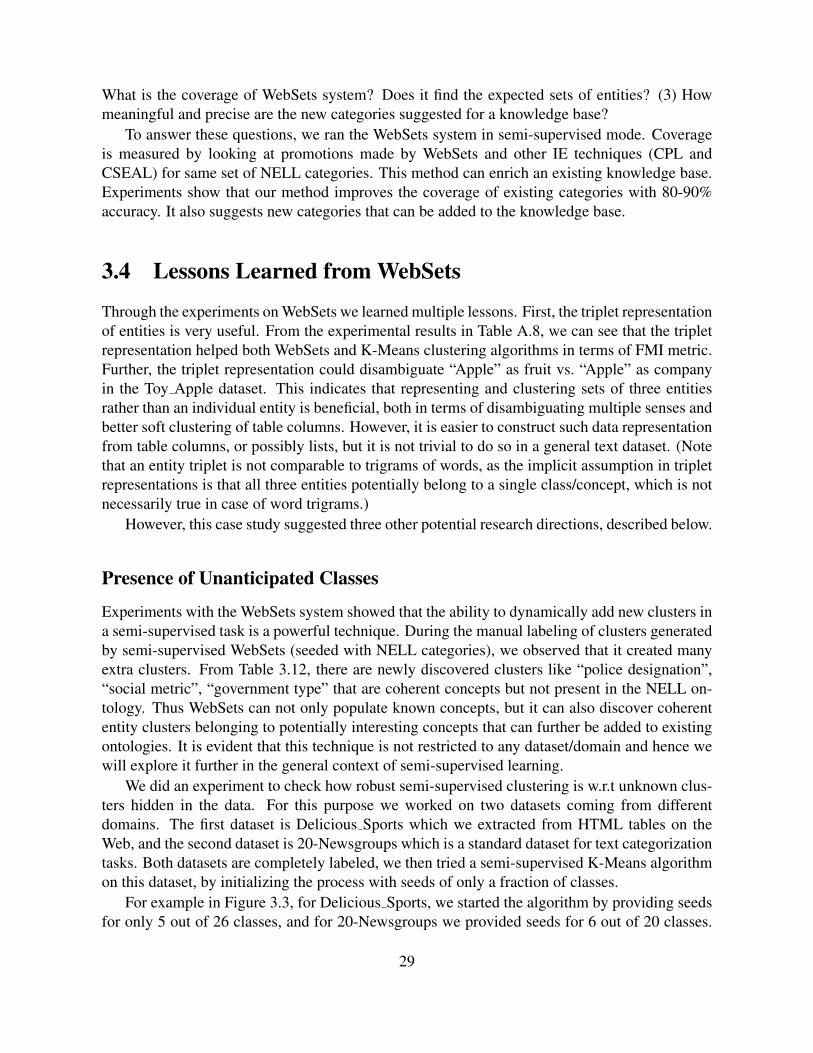
What is the coverage of WebSets system? Does it find the expected sets of entities? (3) Howmeaningful and precise are the new categories suggested for a knowledge base?

To answer these questions, we ran the WebSets system in semi-supervised mode. Coverageis measured by looking at promotions made by WebSets and other IE techniques (CPL andCSEAL) for same set of NELL categories. This method can enrich an existing knowledge base.Experiments show that our method improves the coverage of existing categories with 80-90%accuracy. It also suggests new categories that can be added to the knowledge base.

3.4 Lessons Learned from WebSets

Through the experiments on WebSets we learned multiple lessons. First, the triplet representationof entities is very useful. From the experimental results in Table A.8, we can see that the tripletrepresentation helped both WebSets and K-Means clustering algorithms in terms of FMI metric.Further, the triplet representation could disambiguate “Apple” as fruit vs. “Apple” as companyin the Toy Apple dataset. This indicates that representing and clustering sets of three entitiesrather than an individual entity is beneficial, both in terms of disambiguating multiple senses andbetter soft clustering of table columns. However, it is easier to construct such data representationfrom table columns, or possibly lists, but it is not trivial to do so in a general text dataset. (Notethat an entity triplet is not comparable to trigrams of words, as the implicit assumption in tripletrepresentations is that all three entities potentially belong to a single class/concept, which is notnecessarily true in case of word trigrams.)

However, this case study suggested three other potential research directions, described below.

Presence of Unanticipated Classes

Experiments with the WebSets system showed that the ability to dynamically add new clusters ina semi-supervised task is a powerful technique. During the manual labeling of clusters generatedby semi-supervised WebSets (seeded with NELL categories), we observed that it created manyextra clusters. From Table 3.12, there are newly discovered clusters like “police designation”,“social metric”, “government type” that are coherent concepts but not present in the NELL on-tology. Thus WebSets can not only populate known concepts, but it can also discover coherententity clusters belonging to potentially interesting concepts that can further be added to existingontologies. It is evident that this technique is not restricted to any dataset/domain and hence wewill explore it further in the general context of semi-supervised learning.

We did an experiment to check how robust semi-supervised clustering is w.r.t unknown clus-ters hidden in the data. For this purpose we worked on two datasets coming from differentdomains. The first dataset is Delicious Sports which we extracted from HTML tables on theWeb, and the second dataset is 20-Newsgroups which is a standard dataset for text categorizationtasks. Both datasets are completely labeled, we then tried a semi-supervised K-Means algorithmon this dataset, by initializing the process with seeds of only a fraction of classes.

For example in Figure 3.3, for Delicious Sports, we started the algorithm by providing seedsfor only 5 out of 26 classes, and for 20-Newsgroups we provided seeds for 6 out of 20 classes.

29

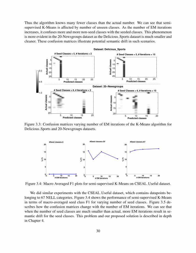
Thus the algorithm knows many fewer classes than the actual number. We can see that semi-supervised K-Means is affected by number of unseen classes. As the number of EM iterationsincreases, it confuses more and more non-seed classes with the seeded classes. This phenomenonis more evident in the 20-Newsgroups dataset as the Delicious Sports dataset is much smaller andcleaner. These confusion matrices illustrate potential semantic drift in such scenarios.

# Seed Classes = 5, # Iterations = 2

Predicted classes

Actu

al

cla

ss

es

5 10 15 20 25

5

10

15

20

25

# Seed Classes = 5, # Iterations = 15

Predicted classes

Actu

al

cla

ss

es

5 10 15 20 25

5

10

15

20

25

# Seed Classes = 6, # Iterations = 2

Predicted classes

Actu

al cla

sses

5 10 15 20

5

10

15

20

# Seed Classes = 6, # Iterations = 15

Predicted classes

Actu

al cla

sses

5 10 15 20

5

10

15

20

1.0

0.5

0.0

Dataset: 20−Newsgroups

Dataset: Delicious_Sports

Figure 3.3: Confusion matrices varying number of EM iterations of the K-Means algorithm forDelicious Sports and 20-Newsgroups datasets.

0 5 10 15 200

5

10

15

20

# EM Iterations

% F

1

0 5 10 15 200

5

10

15

20

# EM Iterations

% F

1

0 5 10 15 200

5

10

15

20

# EM Iterations

% F

1

#Seed classes=20 #Seed classes=67#Seed classes=5

Figure 3.4: Macro Averaged F1 plots for semi-supervised K-Means on CSEAL Useful dataset.

We did similar experiments with the CSEAL Useful dataset, which contains datapoints be-longing to 67 NELL categories. Figure 3.4 shows the performance of semi-supervised K-Meansin terms of macro-averaged seed class F1 for varying number of seed classes. Figure 3.5 de-scribes how the confusion matrices change with the number of EM iterations. We can see thatwhen the number of seed classes are much smaller than actual, more EM iterations result in se-mantic drift for the seed classes. This problem and our proposed solution is described in depthin Chapter 4.

30

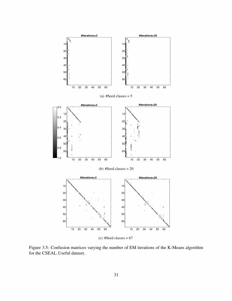
#Iterations=2

10 20 30 40 50 60

10

20

30

40

50

60

#Iterations=20

10 20 30 40 50 60

10

20

30

40

50

60

(a) #Seed classes = 5

#Iterations=2

10 20 30 40 50 60

10

20

30

40

50

60

#Iterations=20

10 20 30 40 50 60

10

20

30

40

50

60

1.0

0.8

0.6

0.4

0.2

0.0

(b) #Seed classes = 20

#Iterations=2

10 20 30 40 50 60

10

20

30

40

50

60

#Iterations=20

10 20 30 40 50 60

10

20

30

40

50

60

(c) #Seed classes = 67

Figure 3.5: Confusion matrices varying the number of EM iterations of the K-Means algorithmfor the CSEAL Useful dataset.

31

Multiple Data ViewsFor many information extraction tasks, including the knowledge base population for NELL, anoun phrase can be represented by features extracted from different kinds of data, e.g., occur-rences of a noun phrases with text contexts, in HTML table columns, and morphological featurescan be considered as three different data views. In the WebSets system, we can construct multi-view features by representing each noun-phrase by 1) a set of co-occurring noun-phrases, 2) aset of table columns it appears in, 3) a set of hypernyms it appears with in the context of Hearstpatterns, and 4) a set of domains it is extracted from. All these clues are useful and give us theinformation that can be leveraged to classify the noun-phrase more effectively.

In Chapter 5, we describe semi-supervised methods that can leverage multiple data views andsolve a constrained optimization problem for each datapoint, to output labels that are consistentin terms of evidence from multiple views.

Leveraging Ontological ConstraintsIn the semi-supervised WebSets experiment, we only use the facts present in NELL KB as initialseeds. However, one can also use the ontology of classes and constraints between the classes toimprove this kind of learning, e.g., the ontology can give us information of the kind: “each noun-phrase that is classified as Mammal should also be classified as Animal” (subset constraint) and“any noun-phrase that is classified as Mammal should not be classified as Reptile” (mutual ex-clusion constraint). In Chapter 6 we will explore techniques that can learn multi-class classifiersleveraging ontological constraints.

32

Chapter 4

Exploratory Learning: Semi-supervisedLearning in the Presence of UnanticipatedClasses

The semi-supervised bottom-up clustering algorithm discussed in the previous chapter can popu-late concepts from NELL as well as discover new clusters of entities that do not belong to any ofthe NELL classes. This revealed a novel problem relevant for such knowledge base populationtasks, i.e., we know about some classes, and some instances of these classes, but the unlabeleddatasets contain examples of many more classes that are not known upfront. Can an algorithmdo both semi-supervised learning for the classes with training data and unsupervised clusteringfor classes without training data? To the best of our knowledge there is no existing techniquethat is targeted to solve this problem.

In this chapter, we propose an Exploratory Learning framework that can make use of limitedsupervision for some of the concepts to populate these known concepts as well as discover newones. This work is published in the proceedings of ECML/PKDD 2013 [128].

4.1 Exploratory EM AlgorithmIn multiclass semi-supervised learning (SSL), it is sometimes the case that the number of

classes present in the data is not known, and hence no labeled examples are provided for someclasses. In this section we present variants of well-known semi-supervised multiclass learningmethods that are robust when the data contains an unknown number of classes. In particular, wepropose an “exploratory” extension of expectation-maximization (EM) that explores differentnumbers of classes while learning.

Algorithm 3 presents a generic Exploratory EM algorithm (without specifying the modelbeing used). There are two main differences between the algorithm and standard classification-EM approaches to SSL. First, in the E step, each of the unlabeled datapoints x is either assignedto one of the existing classes, or to a newly-created class. The intuition we use is that a new classshould be introduced to hold x when the probability of x belonging to existing classes is closeto uniform. This suggests that x is not a good fit to any of the existing classes, and that adding

33

x to any existing class will lower the total data likelihood substantially. Second, in the M-stepof iteration t, we choose either the model proposed by Exploratory EM method which mighthave more classes than the previous iteration t− 1, or the baseline version with same number ofclasses as iteration t − 1. This choice is based on whether exploratory model satisfies a modelselection criterion in terms of increased data likelihood and model complexity.

4.1.1 DiscussionLet us discuss the applicability of this algorithm for clustering as well as classification tasks.Notice that Algorithm 3 reverts to an unsupervised clustering method if X l is empty, and revertsto a supervised generative learner if Xu is empty. Likewise, if no new classes are generated,then it behaves as a multiclass SSL method; for instance, if the classes are well-separated andX l contains enough labels for every class to approximate these classes, then it is unlikely thatthe criterion of nearly-uniform class probabilities will be met, and the algorithm reverts to SSL.Henceforth we will use the terms “class” and “cluster” interchangeably.

Friedman [47] proposed the Structural EM algorithm that combines the standard EM algo-rithm, which optimizes parameters, with structure search for model selection. This algorithmlearns networks based on penalized likelihood scores, in the presence of missing data. In eachiteration it evaluates multiple models based on the expected scores of models with missing data,and selects the model with best expected score. This algorithm converges at local maxima forpenalized log likelihood (the score includes penalty for increased model complexity). Similarto Structural EM, in each iteration of Algorithm 3, we evaluate two models, one with and onewithout adding extra classes. These two models are scored using a model selection criterion likeAIC or BIC, and the model with best penalized data likelihood score is selected in each iteration.Hence we can say that, similar to Structural EM, the Exploratory EM algorithm will converge atlocal maxima for penalized log data likelihood.

34

Algorithm 3 EM algorithm for exploratory learning with model selection.1: function Exploratory EM (X l, Y l, Xu, C1 . . . Ck): Ck+1 . . . Ck+m, θk+m, Y u

2: Input: X l labeled data points; Y l labels of X l; Xu unlabeled data points; C1 . . . Ck set of knownclasses to which x’s belong.

3: Output: Ck+1 . . . Cm newly-discovered classes; θ1, . . . , θk+m parameters for k seed and mnewly added classes; Y u labels for Xu

Initialize classifiers θj for class Cj using seeds provided for Cj4: θ0

1 . . . θ0k = argmaxθL(X

l, Y l)5: while class assignments AND #classes not converged do6: kold is the #classes before E step.7: kcur is the current #classes.8: Log-likelihood BaseLL = logP (X|θ(t)

kold)

E step: (Iteration t) Classify each datapoint at each level9: for i = 1 to |Xu| do

10: Find P (Cj |Xi, θ(t)1 , . . . , θ

(t)kcur

) for all labels 1 ≤ j ≤ kcur11: if nearlyUniform(P (C1|Xi), . . . , P (Ckcur |Xi)) then12: Increment kcur; Let Ckcur be the new class.13: Label Xi with Ckcur in Y u, and compute parameters θ(t)

kcurfor the new class.

14: else15: Assign Xi to (argmaxCjP (Cj |Xi)) in Y u where 1 ≤ j ≤ kcur16: end if17: end for18: knew = kcur is the #classes after E step.19: Log-likelihood ExploreLL = logP (X|θ(t)

knew)

M step: Recompute model parameters based on Y (t) 20: if Model selection criterion (kold, BaseLL, knew, ExploreLL) selects exploratory model then

Adopt the new model with knew classes21: θ

(t+1)knew

= argmaxθL(Xl, Y l, Xu, Y u(t)|θ(t)

knew)

22: elseKeep the old model with kold classes

23: θ(t+1)kold

= argmaxθL(Xl, Y l, Xu, Y u(t)|θ(t)

kold)

24: end if25: end while26: end function

35

4.1.2 Model SelectionAny training error based model selection can be used in this framework e.g., BIC, AIC and AICc.Burnham and Anderson [18] have experimented with the AIC criteria and proposed AICc fordatasets where the number of datapoints is less than 40 times number of features. The formulaefor scoring a model using each of the three criteria that we tried are:

BIC(g) = −2 ∗ L(g) + v ∗ ln(n) (4.1)AIC(g) = −2 ∗ L(g) + 2 ∗ v (4.2)AICc(g) = AIC(g) + 2 ∗ v ∗ (v + 1)/(n− v − 1) (4.3)

where g is the model being evaluated, L(g) is the log-likelihood of the data given g, v is thenumber of free parameters of the model and n is the number of data-points, so when comparingtwo models, a lower value is preferred. The extended Akaike information criterion (AICc) suitedbest for our experiments since our datasets have large number of features and a smaller numberof data points. With the AICc criterion, the objective function being optimized is:

maxm,θ1...θm,m≥k

Log Data Likelihood−Model penalty

i.e., maxm,θ1...θm,m≥k

logP (X|θ1, . . . , θm) − v + (v ∗ (v + 1)/(n− v − 1))(4.4)

Here, k is the number of seed classes given as input to the algorithm and m is the number ofclasses in the resultant model (m ≥ k).

4.1.3 Exploratory EM using Different Language ModelsIn this section we will consider variants of Exploratory EM algorithm with different languagemodels. The choice of language model decides the method used in Algorithm 3 Line 10, 21 and23.

Semi-Supervised Naive Bayes: Nigam et al. [98] proposed an EM-based semi-supervised ver-sion of multinomial Naive Bayes. In this model P (Cj|x) ∝ P (x|Cj)∗P (Cj), for each unlabeledpoint x. The probability P (x|Cj) is estimated by treating each feature in x as an independentdraw from a class-specific multinomial. In document classification, the features are word occur-rences, and the number of outcomes of the multinomial is the vocabulary size. This method canbe naturally used as an instance of Exploratory EM, using the multinomial model to computeP (Cj|x) in Algorithm 3 Line 10. The M step is also trivial, requiring only estimates of P (w|Cj)for each word/feature w.

Seeded K-Means: It has often been observed that K-Means and EM are algorithmically similar.Basu and Mooney [9] proposed a seeded version of K-Means, which is very analogous to Nigamet al’s semi-supervised Naive Bayes, as another technique for semi-supervised learning. SeededK-Means takes as input a number of clusters, and seed examples for each cluster. The seedsare used to define an initial set of cluster centroids, and then the algorithm iterates between an

36

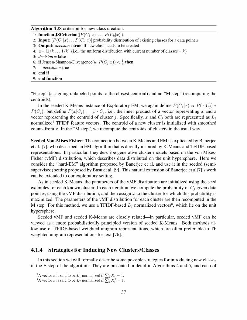
Algorithm 4 JS criterion for new class creation.1: function JSCriterion([P (C1|x) . . . P (Ck|x)]):2: Input: [P (C1|x) . . . P (Ck|x)] probability distribution of existing classes for a data point x3: Output: decision : true iff new class needs to be created4: u = [1/k . . . 1/k] i.e., the uniform distribution with current number of classes = k5: decision = false6: if Jensen-Shannon-Divergence(u, P (Cj |x)) < 1

k then7: decision = true8: end if9: end function

“E step” (assigning unlabeled points to the closest centroid) and an “M step” (recomputing thecentroids).

In the seeded K-Means instance of Exploratory EM, we again define P (Cj|x) ∝ P (x|Cj) ∗P (Cj), but define P (x|Cj) = x · Cj , i.e., the inner product of a vector representing x and avector representing the centroid of cluster j. Specifically, x and Cj both are represented as L1

normalized7 TFIDF feature vectors. The centroid of a new cluster is initialized with smoothedcounts from x. In the “M step”, we recompute the centroids of clusters in the usual way.

Seeded Von-Mises Fisher: The connection between K-Means and EM is explicated by Banerjeeet al. [7], who described an EM algorithm that is directly inspired by K-Means and TFIDF-basedrepresentations. In particular, they describe generative cluster models based on the von Mises-Fisher (vMF) distribution, which describes data distributed on the unit hypersphere. Here weconsider the “hard-EM” algorithm proposed by Banerjee et al, and use it in the seeded (semi-supervised) setting proposed by Basu et al. [9]. This natural extension of Banerjee et al[7]’s workcan be extended to our exploratory setting.

As in seeded K-Means, the parameters of the vMF distribution are initialized using the seedexamples for each known cluster. In each iteration, we compute the probability of Cj given datapoint x, using the vMF distribution, and then assign x to the cluster for which this probability ismaximized. The parameters of the vMF distribution for each cluster are then recomputed in theM step. For this method, we use a TFIDF-based L2 normalized vectors8, which lie on the unithypersphere.

Seeded vMF and seeded K-Means are closely related—in particular, seeded vMF can beviewed as a more probabilistically principled version of seeded K-Means. Both methods al-low use of TFIDF-based weighted unigram representations, which are often preferable to TFweighted unigram representations for text [76].

4.1.4 Strategies for Inducing New Clusters/Classes

In this section we will formally describe some possible strategies for introducing new classesin the E step of the algorithm. They are presented in detail in Algorithms 4 and 5, and each of

7A vector x is said to be L1 normalized if∑

iXi = 1.8A vector x is said to be L2 normalized if

∑iX

2i = 1.

37

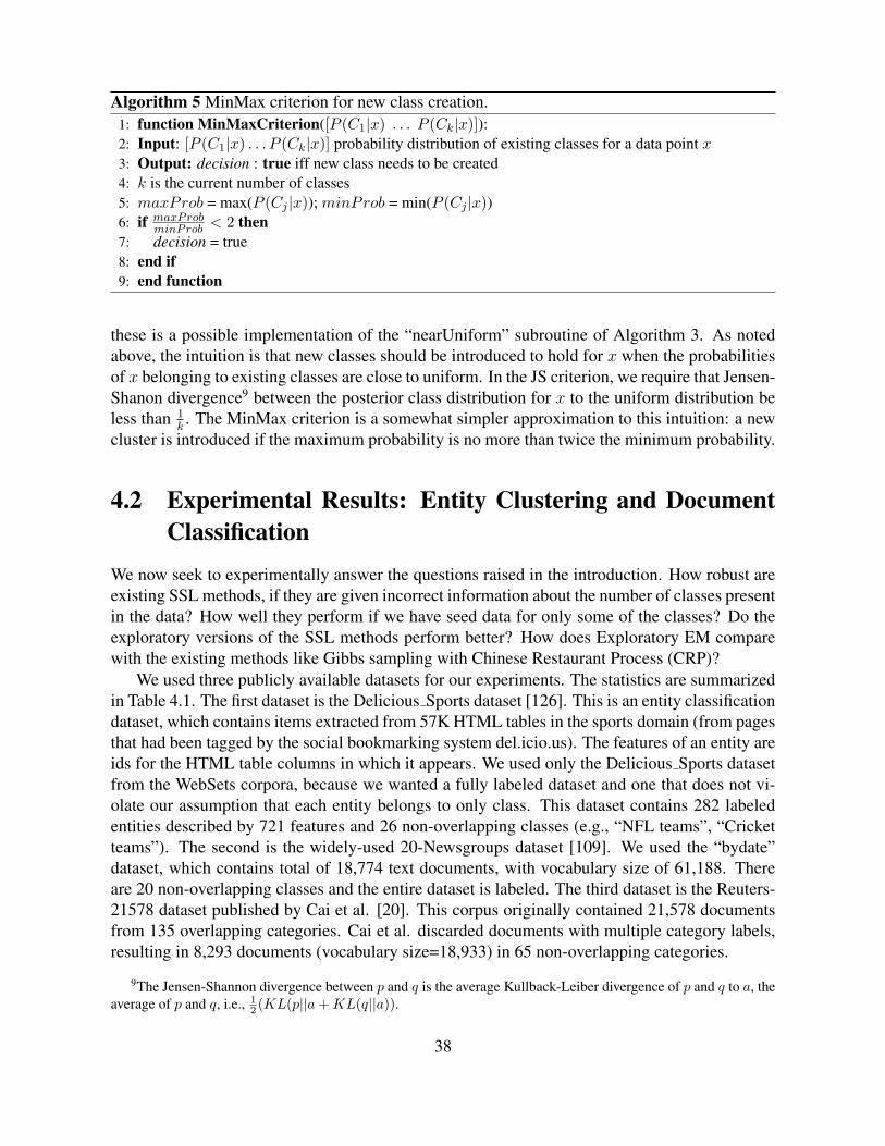
Algorithm 5 MinMax criterion for new class creation.1: function MinMaxCriterion([P (C1|x) . . . P (Ck|x)]):2: Input: [P (C1|x) . . . P (Ck|x)] probability distribution of existing classes for a data point x3: Output: decision : true iff new class needs to be created4: k is the current number of classes5: maxProb = max(P (Cj |x)); minProb = min(P (Cj |x))6: if maxProbminProb < 2 then7: decision = true8: end if9: end function

these is a possible implementation of the “nearUniform” subroutine of Algorithm 3. As notedabove, the intuition is that new classes should be introduced to hold for x when the probabilitiesof x belonging to existing classes are close to uniform. In the JS criterion, we require that Jensen-Shanon divergence9 between the posterior class distribution for x to the uniform distribution beless than 1

k. The MinMax criterion is a somewhat simpler approximation to this intuition: a new

cluster is introduced if the maximum probability is no more than twice the minimum probability.

4.2 Experimental Results: Entity Clustering and DocumentClassification

We now seek to experimentally answer the questions raised in the introduction. How robust areexisting SSL methods, if they are given incorrect information about the number of classes presentin the data? How well they perform if we have seed data for only some of the classes? Do theexploratory versions of the SSL methods perform better? How does Exploratory EM comparewith the existing methods like Gibbs sampling with Chinese Restaurant Process (CRP)?

We used three publicly available datasets for our experiments. The statistics are summarizedin Table 4.1. The first dataset is the Delicious Sports dataset [126]. This is an entity classificationdataset, which contains items extracted from 57K HTML tables in the sports domain (from pagesthat had been tagged by the social bookmarking system del.icio.us). The features of an entity areids for the HTML table columns in which it appears. We used only the Delicious Sports datasetfrom the WebSets corpora, because we wanted a fully labeled dataset and one that does not vi-olate our assumption that each entity belongs to only class. This dataset contains 282 labeledentities described by 721 features and 26 non-overlapping classes (e.g., “NFL teams”, “Cricketteams”). The second is the widely-used 20-Newsgroups dataset [109]. We used the “bydate”dataset, which contains total of 18,774 text documents, with vocabulary size of 61,188. Thereare 20 non-overlapping classes and the entire dataset is labeled. The third dataset is the Reuters-21578 dataset published by Cai et al. [20]. This corpus originally contained 21,578 documentsfrom 135 overlapping categories. Cai et al. discarded documents with multiple category labels,resulting in 8,293 documents (vocabulary size=18,933) in 65 non-overlapping categories.

9The Jensen-Shannon divergence between p and q is the average Kullback-Leiber divergence of p and q to a, theaverage of p and q, i.e., 1

2 (KL(p||a+KL(q||a)).

38

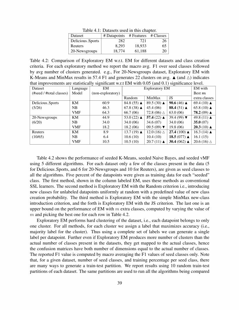
Table 4.1: Datasets used in this chapter.Dataset # Datapoints # Features # ClassesDelicious Sports 282 721 26Reuters 8,293 18,933 6520-Newsgroups 18,774 61,188 20

Table 4.2: Comparison of Exploratory EM w.r.t. EM for different datasets and class creationcriteria. For each exploratory method we report the macro avg. F1 over seed classes followedby avg number of clusters generated. e.g., For 20-Newsgroups dataset, Exploratory EM withK-Means and MinMax results in 57.4 F1 and generates 22 clusters on avg. N (and M) indicatesthat improvements are statistically significant w.r.t EM with 0.05 (and 0.1) significance level.

Dataset Language EM Exploratory EM EM with(#seed / #total classes) Model (non-exploratory) Best m

Random MinMax JS extra classesDelicious Sports KM 60.9 84.8 (55) N 89.5 (30) N 90.6 (46) N 69.4 (10) N(5/26) NB 46.3 67.8 (38) N 45.4 (06) 88.4 (51) N 65.8 (10) N

VMF 64.3 66.7 (06) 72.8 (06) M 63.0 (06) 78.2 (09) N20-Newsgroups KM 44.9 53.0 (22) N 57.4 (22) N 39.4 (99) H 49.8 (11) N(6/20) NB 34.0 34.0 (06) 34.6 (07) 34.0 (06) 35.0 (07)

VMF 18.2 18.2 (06) 09.5 (09) H 19.8 (06) 20.3 (10) NReuters KM 8.9 13.7 (19) N 12.0 (16) M 27.4 (100) N 16.3 (14) N(10/65) NB 6.4 10.6 (10) 10.4 (10) 18.5 (077) N 16.1 (15)

VMF 10.5 10.5 (10) 20.7 (11) N 30.4 (062) N 20.6 (16) M

Table 4.2 shows the performance of seeded K-Means, seeded Naive Bayes, and seeded vMFusing 5 different algorithms. For each dataset only a few of the classes present in the data (5for Delicious Sports, and 6 for 20-Newsgroups and 10 for Reuters), are given as seed classes toall the algorithms. Five percent of the datapoints were given as training data for each “seeded”class. The first method, shown in the column labeled EM, uses these methods as conventionalSSL learners. The second method is Exploratory EM with the Random criterion i.e., introducingnew classes for unlabeled datapoints uniformly at random with a predefined value of new classcreation probability. The third method is Exploratory EM with the simple MinMax new-classintroduction criterion, and the forth is Exploratory EM with the JS criterion. The last one is anupper bound on the performance of EM with m extra classes, computed by varying the value ofm and picking the best one for each row in Table 4.2.

Exploratory EM performs hard clustering of the dataset, i.e., each datapoint belongs to onlyone cluster. For all methods, for each cluster we assign a label that maximizes accuracy (i.e.,majority label for the cluster). Thus using a complete set of labels we can generate a singlelabel per datapoint. Further even if Exploratory EM produces more number of clusters than theactual number of classes present in the datasets, they get mapped to the actual classes, hencethe confusion matrices have both number of dimensions equal to the actual number of classes.The reported F1 value is computed by macro averaging the F1 values of seed classes only. Notethat, for a given dataset, number of seed classes, and training percentage per seed class, thereare many ways to generate a train-test partition. We report results using 10 random train-testpartitions of each dataset. The same partitions are used to run all the algorithms being compared

39

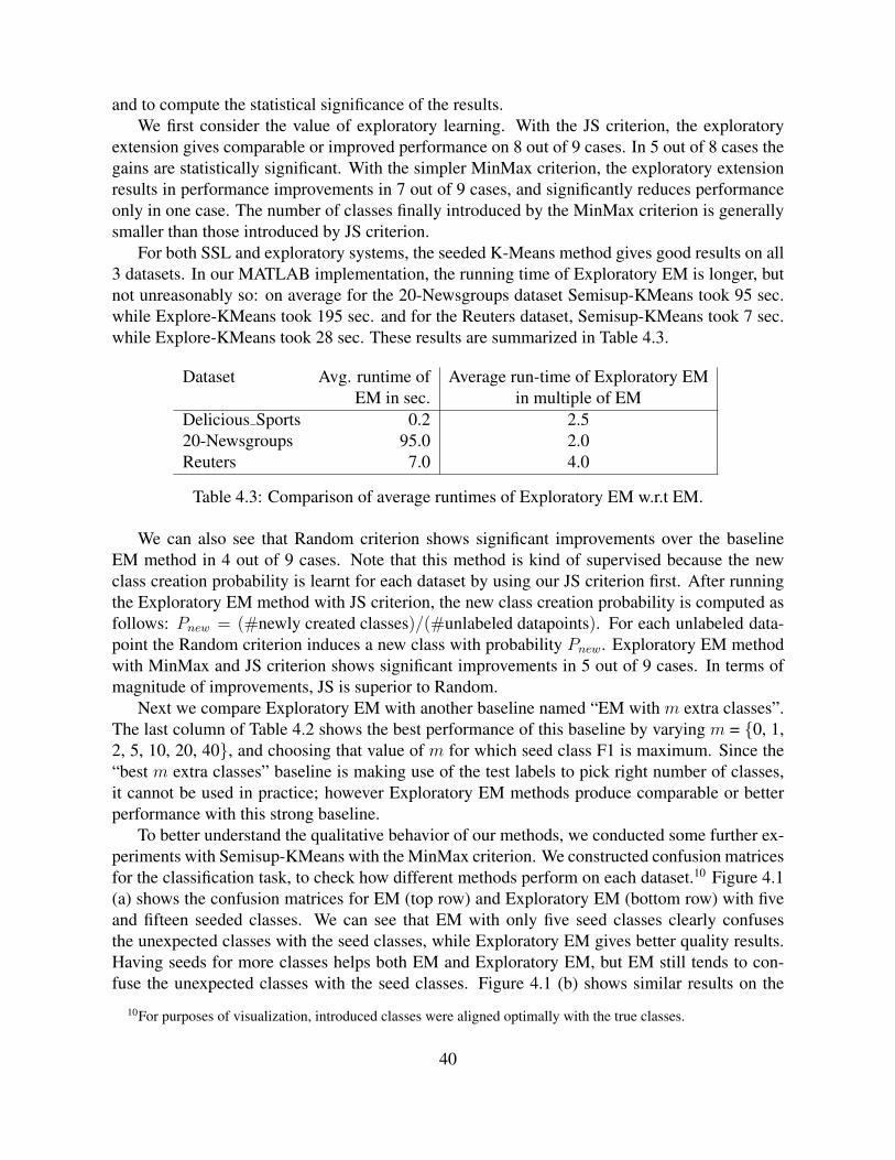
and to compute the statistical significance of the results.We first consider the value of exploratory learning. With the JS criterion, the exploratory

extension gives comparable or improved performance on 8 out of 9 cases. In 5 out of 8 cases thegains are statistically significant. With the simpler MinMax criterion, the exploratory extensionresults in performance improvements in 7 out of 9 cases, and significantly reduces performanceonly in one case. The number of classes finally introduced by the MinMax criterion is generallysmaller than those introduced by JS criterion.

For both SSL and exploratory systems, the seeded K-Means method gives good results on all3 datasets. In our MATLAB implementation, the running time of Exploratory EM is longer, butnot unreasonably so: on average for the 20-Newsgroups dataset Semisup-KMeans took 95 sec.while Explore-KMeans took 195 sec. and for the Reuters dataset, Semisup-KMeans took 7 sec.while Explore-KMeans took 28 sec. These results are summarized in Table 4.3.

Dataset Avg. runtime of Average run-time of Exploratory EMEM in sec. in multiple of EM

Delicious Sports 0.2 2.520-Newsgroups 95.0 2.0Reuters 7.0 4.0

Table 4.3: Comparison of average runtimes of Exploratory EM w.r.t EM.

We can also see that Random criterion shows significant improvements over the baselineEM method in 4 out of 9 cases. Note that this method is kind of supervised because the newclass creation probability is learnt for each dataset by using our JS criterion first. After runningthe Exploratory EM method with JS criterion, the new class creation probability is computed asfollows: Pnew = (#newly created classes)/(#unlabeled datapoints). For each unlabeled data-point the Random criterion induces a new class with probability Pnew. Exploratory EM methodwith MinMax and JS criterion shows significant improvements in 5 out of 9 cases. In terms ofmagnitude of improvements, JS is superior to Random.

Next we compare Exploratory EM with another baseline named “EM with m extra classes”.The last column of Table 4.2 shows the best performance of this baseline by varying m = 0, 1,2, 5, 10, 20, 40, and choosing that value of m for which seed class F1 is maximum. Since the“best m extra classes” baseline is making use of the test labels to pick right number of classes,it cannot be used in practice; however Exploratory EM methods produce comparable or betterperformance with this strong baseline.

To better understand the qualitative behavior of our methods, we conducted some further ex-periments with Semisup-KMeans with the MinMax criterion. We constructed confusion matricesfor the classification task, to check how different methods perform on each dataset.10 Figure 4.1(a) shows the confusion matrices for EM (top row) and Exploratory EM (bottom row) with fiveand fifteen seeded classes. We can see that EM with only five seed classes clearly confusesthe unexpected classes with the seed classes, while Exploratory EM gives better quality results.Having seeds for more classes helps both EM and Exploratory EM, but EM still tends to con-fuse the unexpected classes with the seed classes. Figure 4.1 (b) shows similar results on the

10For purposes of visualization, introduced classes were aligned optimally with the true classes.

40

20-Newsgroups dataset, but shows the confusion matrix after 1 iteration and after 15 iterationsof EM. It shows that EM after 15 iterations has made limited progress in improving its classifierwhen compared to Exploratory EM.

Finally, we compare the two class creation criteria, and show a somewhat larger range ofseeded classes, ranging from 5 to 15 (out of 20 actual classes). In Figure 4.2 each of theconfusion-matrices is annotated with the strategy, the number of seed classes and the number ofclasses produced. (For example, plot “MinMax-C5(23)” describes Explore-KMeans with Min-Max criterion and 5 seed classes which produces 23 clusters.) We can see that MinMax criterionusually produces a more reasonable number of clusters, closer to the ideal value of 20; however,the performance of the JS method in terms of seed class accuracy is comparable to the MinMaxmethod.

These trends are also shown quantitatively in Figure 4.3, which shows the result of varying thenumber of seeded classes (with five seeds per class) for Explore-KMeans and Semisup-KMeans;the top shows the effect on F1, and the bottom shows the effect on the number of classes produced(for Explore-KMeans only). Figure 4.4 shows a similar effect on the Delicious Sports dataset:here we systematically vary the number of seeded classes (using 5 seeds per seeded class, onthe top), and also vary the number of seeds per class (using 10 seeded classes, on the bottom.)The left-hand side compares the F1 for Semisup-KMeans and Explore-KMeans, and the right-hand side shows the number of classes produced by Explore-KMeans. For all parameter settings,Explore-KMeans is better than or comparable to Semisup-KMeans in terms of F1 on seed classes.

4.3 Evaluation on Non-seed ClassesTable 4.4 presents the results for macro-averaged F1 scores on seeded and unanticipated classes.Best scores in each row are bold-faced. We can see that on a relatively easier dataset like Deli-cious Sports which has clearly separable classes, our methods could easily discover good qualityextra clusters corresponding to unanticipated classes. However, as the complexity of classifica-tion task increases, our methods prove to be less effective. E.g., Reuters dataset has less clearlyseparable classes, and only small fraction of them are given as input to the algorithm. For thistask Exploratory EM could induce many new clusters but they do not directly correspond to theideal class definitions in the test data resulting in low F1 scores on unanticipated classes.

Further the Exploratory EM method resulted in better F1 score on unanticipated classes whencompared to EM with best m-extra classes. Thus we observe from Tables 4.2 and 4.4 that dy-namically adding new clusters of datapoints that do not belong to any of the known classes doesreduce semantic drift of existing classes even if the newly added clusters are not meaningful (thenewly added clusters might not have 1 to 1 correspondence with the unanticipated classes).

4.4 Additional ResultsWe later created four entity classification datasets using subsets of NELL ontology (see Figure7.1) and generated feature vectors using occurrences with text patterns and HTML table columnsin the ClueWeb09 corpus. Description of these four datasets can be found in Section 7.4. We

41

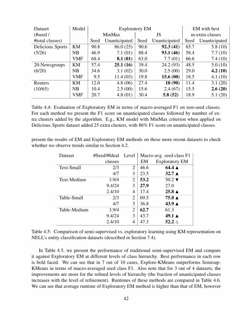
Dataset Model Exploratory EM EM with best(#seed / MinMax JS m-extra classes#total classes) Seed Unanticipated Seed Unanticipated Seed UnanticipatedDelicious Sports KM 90.8 86.0 (25) 90.6 92.3 (41) 65.7 5.8 (10)(5/26) NB 46.9 7.1 (01) 88.4 93.1 (46) 58.4 7.7 (10)

VMF 68.4 8.1 (01) 63.0 7.7 (01) 66.6 7.4 (10)20-Newsgroups KM 57.4 25.1 (16) 39.4 24.2 (93) 48.5 5.0 (10)(6/20) NB 34.6 3.1 (02) 30.0 2.5 (00) 29.0 4.2 (10)

VMF 9.5 11.4 (03) 19.8 15.6 (00) 18.5 4.1 (10)Reuters KM 12.0 4.8 (06) 27.4 10 (90) 11.4 3.1 (20)(10/65) NB 10.4 2.5 (00) 15.6 2.4 (67) 15.5 2.6 (20)

VMF 20.7 4.8 (01) 30.4 5.8 (52) 18.9 5.1 (20)

Table 4.4: Evaluation of Exploratory EM in terms of macro-averaged F1 on non-seed classes.For each method we present the F1 score on unanticipated classes followed by number of ex-tra clusters added by the algorithm. E.g., KM model with MinMax criterion when applied onDelicious Sports dataset added 25 extra clusters, with 86% F1 score on unanticipated classes.

present the results of EM and Exploratory EM methods on these more recent datasets to checkwhether we observe trends similar to Section 4.2.

Dataset #Seed/#Ideal Level Macro-avg. seed class F1classes EM Exploratory EM

Text-Small 2/3 2 46.6 64.4 N4/7 3 23.5 32.7 N

Text-Medium 3.9/4 2 53.2 50.2 H9.4/24 3 27.9 27.02.4/10 4 17.4 25.8 N

Table-Small 2/3 2 69.5 75.8 N4/7 3 36.8 43.9 N

Table-Medium 3.9/4 2 62.7 61.39.4/24 3 43.7 49.1 N2.4/10 4 47.3 52.2 M

Table 4.5: Comparison of semi-supervised vs. exploratory learning using KM representation onNELL’s entity classification datasets (described in Section 7.4).

In Table 4.5, we present the performance of traditional semi-supervised EM and compareit against Exploratory EM at different levels of class hierarchy. Best performance in each rowis bold faced. We can see that in 7 out of 10 cases, Explore-KMeans outperforms Semisup-KMeans in terms of macro-averaged seed class F1. Also note that for 3 out of 4 datasets, theimprovements are more for the refined levels of hierarchy (the fraction of unanticipated classesincreases with the level of refinement). Runtimes of these methods are compared in Table 4.6.We can see that average runtime of Exploratory EM method is higher than that of EM, however

42

not unreasonably so.

Dataset Avg. runtime of Average run-time of Exploratory EMEM in sec. in multiple of FLAT-EM

Text-Small 53 8Text-Medium 524 5Table-Small 50 3Table-Medium 5932 4

Table 4.6: Comparison of average runtimes of Exploratory EM w.r.t EM.

4.5 Experiments with Chinese Restaurant ProcessThe Exploratory EM method is broadly similar to non-parametric Bayesian methods, such asthe Chinese Restaurant Process (CRP) [11]. CRP is often used in non-parametric models (e.g.,topic models) that are based on Gibbs sampling, and indeed, since it is straightforward to replaceEM with Gibbs-sampling, one can use this approach to estimate the parameters of any of themodels considered here (i.e., multinomial Naive Bayes, K-Means, and the von Mises-Fisherdistribution). Algorithm 6 presents a seeded version of a Gibbs sampler based on this idea. Inbrief, Algorithm 6 starts with a classifier trained on the labeled data. Collapsed Gibbs samplingis then performed over the latent labels of unlabeled data, incorporating the CRP into the Gibbssampling to introduce new classes. (In fact, we use block sampling for these variables, to makethe method more similar to the EM variants.)

The subroutine CRPPick is explained in Algorithm 7. This function concatenates the pos-terior distribution of classes given a datapoint with the new class creation probability or con-centration parameter of CRP, renormalizes this vector and then samples a label from this newdistribution. If the new class is selected then the number of classes is incremented by one.

Note that this algorithm is naturally “exploratory”, in our sense, as it can produce a numberof classes larger than the number of classes for which seed labels exist. However, unlike ourexploratory EM variants, the introduction of new classes is not driven by examples that are “hardto classify”—i.e., have nearly-uniform posterior probability of membership in existing classes.In the CRP method, the probability of creating a new class depends on the data point, but it doesnot explicitly favor cases where the posterior over existing classes is nearly uniform.

To address this issue, we also implemented a variant of the seeded Gibbs sampler with CRP,in which the examples with nearly-uniform distributions are more likely to be assigned to newclasses. This variant is shown in Algorithm 8, which replaces the routine CRPPick in the Gibbssampler—in brief, we simply scale down the probability of creating a new class by the Jensen-Shannon divergence of the posterior class distribution for x to the uniform distribution. Hencethe probability of creating a new class explicitly depends on how well the given data point fits inone of the existing classes.

Next we compare the performance of CRPGibbs with Explore-KMeans and Semisup-KMeans.We consider two versions of CRP-Gibbs, one using the standard CRP and one using our proposedmodified CRP criterion for new class creation that is sensitive to the near-uniformity of instance’s

43

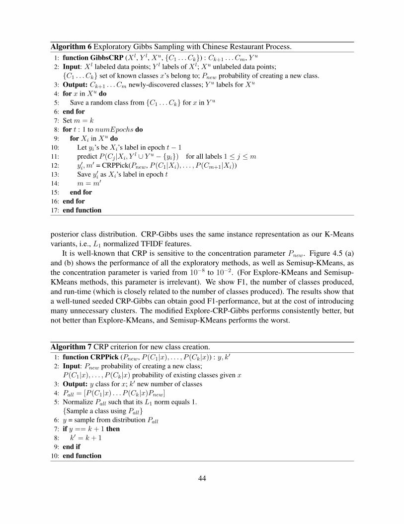
Algorithm 6 Exploratory Gibbs Sampling with Chinese Restaurant Process.1: function GibbsCRP (X l, Y l, Xu, C1 . . . Ck) : Ck+1 . . . Cm, Y u

2: Input: X l labeled data points; Y l labels of X l; Xu unlabeled data points;C1 . . . Ck set of known classes x’s belong to; Pnew probability of creating a new class.

3: Output: Ck+1 . . . Cm newly-discovered classes; Y u labels for Xu

4: for x in Xu do5: Save a random class from C1 . . . Ck for x in Y u

6: end for7: Set m = k8: for t : 1 to numEpochs do9: for Xi in Xu do

10: Let yi’s be Xi’s label in epoch t− 111: predict P (Cj |Xi, Y

l ∪ Y u − yi) for all labels 1 ≤ j ≤ m12: y′i,m

′ = CRPPick(Pnew, P (C1|Xi), . . . , P (Cm+1|Xi))13: Save y′i as Xi’s label in epoch t14: m = m′

15: end for16: end for17: end function

posterior class distribution. CRP-Gibbs uses the same instance representation as our K-Meansvariants, i.e., L1 normalized TFIDF features.

It is well-known that CRP is sensitive to the concentration parameter Pnew . Figure 4.5 (a)and (b) shows the performance of all the exploratory methods, as well as Semisup-KMeans, asthe concentration parameter is varied from 10−8 to 10−2. (For Explore-KMeans and Semisup-KMeans methods, this parameter is irrelevant). We show F1, the number of classes produced,and run-time (which is closely related to the number of classes produced). The results show thata well-tuned seeded CRP-Gibbs can obtain good F1-performance, but at the cost of introducingmany unnecessary clusters. The modified Explore-CRP-Gibbs performs consistently better, butnot better than Explore-KMeans, and Semisup-KMeans performs the worst.

Algorithm 7 CRP criterion for new class creation.1: function CRPPick (Pnew, P (C1|x), . . . , P (Ck|x)) : y, k′

2: Input: Pnew probability of creating a new class;P (C1|x), . . . , P (Ck|x) probability of existing classes given x

3: Output: y class for x; k′ new number of classes4: Pall = [P (C1|x) . . . P (Ck|x)Pnew]5: Normalize Pall such that its L1 norm equals 1.Sample a class using Pall

6: y = sample from distribution Pall7: if y == k + 1 then8: k′ = k + 19: end if

10: end function

44

Algorithm 8 Modified CRP criterion for new class creation.1: function ModCRPPick (Pnew, P (C1|x), . . . , P (Ck|x)) : y, k′

2: Input: Pnew probability of creating a new class;P (C1|x), . . . , P (Ck|x) probability of existing classes given x

3: Output: y class for x; k′ new number of classes4: u = [1/k . . . 1/k] uniform distribution with k classes5: d = Jensen-Shannon-Divergence(u, P (Cj |x))6: q = Pnew

((k)∗d)7: if a coin with bias q is heads then

create a new class and assign to that8: y = k + 1 and k′ = k + 19: else

assign to an existing class10: k′ = k and y = sample from distribution [P (C1|x) . . . P (Ck|x)]11: end if12: end function

45

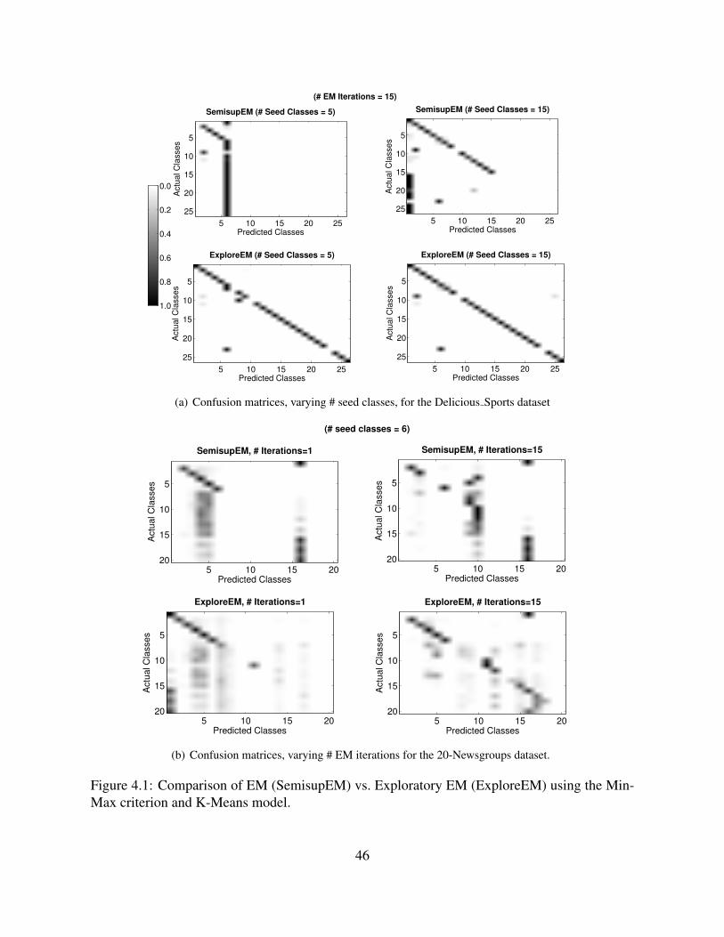
SemisupEM (# Seed Classes = 5)

Predicted Classes

Actu

al C

lasses

5 10 15 20 25

5

10

15

20

25

SemisupEM (# Seed Classes = 15)

Predicted Classes

Actu

al C

lasses

5 10 15 20 25

5

10

15

20

25

ExploreEM (# Seed Classes = 5)

Predicted Classes

Actu

al C

lasses

5 10 15 20 25

5

10

15

20

25

ExploreEM (# Seed Classes = 15)

Predicted Classes

Actu

al C

lasse

s

5 10 15 20 25

5

10

15

20

25

1.0

0.8

0.6

0.4

0.2

0.0

(# EM Iterations = 15)

(a) Confusion matrices, varying # seed classes, for the Delicious Sports dataset

SemisupEM, # Iterations=1

Predicted Classes

Actu

al C

lasse

s

5 10 15 20

5

10

15

20

SemisupEM, # Iterations=15

Predicted Classes

Actu

al C

lasse

s

5 10 15 20

5

10

15

20

ExploreEM, # Iterations=1

Predicted Classes

Actu

al C

lasse

s

5 10 15 20

5

10

15

20

ExploreEM, # Iterations=15

Predicted Classes

Actu

al C

lasse

s

5 10 15 20

5

10

15

20

(# seed classes = 6)

(b) Confusion matrices, varying # EM iterations for the 20-Newsgroups dataset.

Figure 4.1: Comparison of EM (SemisupEM) vs. Exploratory EM (ExploreEM) using the Min-Max criterion and K-Means model.

46

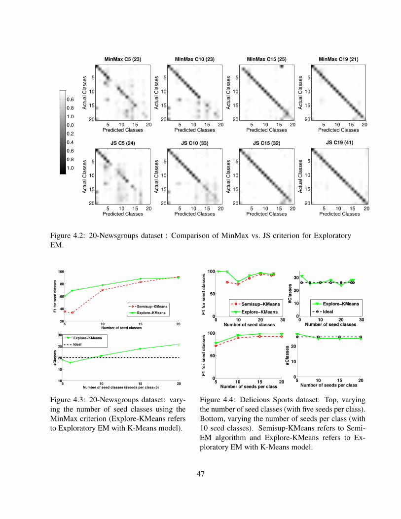
MinMax C5 (23)

Predicted Classes

Actu

al C

lasse

s

5 10 15 20

5

10

15

20

MinMax C10 (23)

Predicted Classes

Actu

al C

lasse

s

5 10 15 20

5

10

15

20

MinMax C15 (25)

Predicted Classes

Actu

al C

lasse

s

5 10 15 20

5

10

15

20

MinMax C19 (21)

Predicted Classes

Actu

al C

lasse

s

5 10 15 20

5

10

15

20

JS C5 (24)

Predicted Classes

Actu

al C

lasse

s

5 10 15 20

5

10

15

20

JS C10 (33)

Predicted Classes

Actu

al C

lasse

s

5 10 15 20

5

10

15

20

JS C15 (32)

Predicted Classes

Actu

al C

lasse

s

5 10 15 20

5

10

15

20

JS C19 (41)

Predicted Classes

Actu

al C

lasse

s

5 10 15 20

5

10

15

20

1.0

0.8

0.6

0.4

0.2

0.0

1.0

0.8

0.6

Figure 4.2: 20-Newsgroups dataset : Comparison of MinMax vs. JS criterion for ExploratoryEM.

5 10 15 2020

40

60

80

100

Number of seed classes

F1

fo

r s

ee

d c

las

se

s

Semisup−KMeans

Explore−KMeans

5 10 15 2010

15

20

25

30

Number of seed classes (#seeds per class=5)

#C

las

se

s

Explore−KMeans

Ideal

Figure 4.3: 20-Newsgroups dataset: vary-ing the number of seed classes using theMinMax criterion (Explore-KMeans refersto Exploratory EM with K-Means model).

0 10 20 300

50

100

Number of seed classes

F1 f

or

seed

cla

sses

Semisup−KMeans

Explore−KMeans

0 10 20 300

10

20

30

Number of seed classes

#C

lasses

Explore−KMeans

Ideal

5 10 15 200

50

100

Number of seeds per class

F1 f

or

seed

cla

sses

5 10 15 200

10

20

Number of seeds per class

#C

lasses

Figure 4.4: Delicious Sports dataset: Top, varyingthe number of seed classes (with five seeds per class).Bottom, varying the number of seeds per class (with10 seed classes). Semisup-KMeans refers to Semi-EM algorithm and Explore-KMeans refers to Ex-ploratory EM with K-Means model.

47

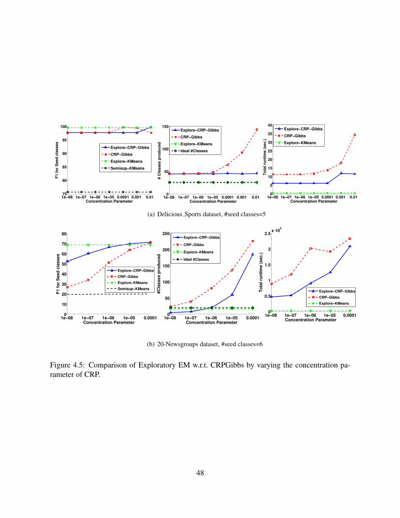
1e−08 1e−07 1e−06 1e−05 0.0001 0.001 0.01 75

80

85

90

95

100

Concentration Parameter

F1

fo

r S

ee

d c

las

se

s

Explore−CRP−Gibbs

CRP−Gibbs

Explore−KMeans

Semisup−KMeans

1e−08 1e−07 1e−06 1e−05 0.0001 0.001 0.01 0

50

100

150

Concentration Parameter

# C

las

se

s p

rod

uc

ed

Explore−CRP−Gibbs

CRP−Gibbs

Explore−KMeans

Ideal #Classes

1e−08 1e−07 1e−06 1e−05 0.0001 0.001 0.01 0

5

10

15

20

25

30

35

40

Concentration Parameter

To

tal

run

tim

e (

se

c.)

Explore−CRP−Gibbs

CRP−Gibbs

Explore−KMeans

(a) Delicious Sports dataset, #seed classes=5

1e−08 1e−07 1e−06 1e−05 0.00010

10

20

30

40

50

60

70

80

Concentration Parameter

F1

fo

r S

ee

d c

las

se

s

Explore−CRP−Gibbs

CRP−Gibbs

Explore−KMeans

Semisup−KMeans

1e−08 1e−07 1e−06 1e−05 0.00010

50

100

150

200

250

Concentration Parameter

#C

las

se

s p

rod

uc

ed

Explore−CRP−Gibbs

CRP−Gibbs

Explore−KMeans

Ideal #Classes

1e−08 1e−07 1e−06 1e−05 0.00010

0.5

1

1.5

2

2.5x 10

4

Concentration Parameter

To

tal

run

tim

e (

se

c.)

Explore−CRP−Gibbs

CRP−Gibbs

Explore−KMeans

(b) 20-Newsgroups dataset, #seed classes=6

Figure 4.5: Comparison of Exploratory EM w.r.t. CRPGibbs by varying the concentration pa-rameter of CRP.

48

4.6 Related Work: Semi-supervised Learning, Negative ClassDiscovery, Topic Detection and Tracking

In this chapter we described and evaluated a novel multiclass SSL method “Exploratory EM”that is more robust when there are unanticipated classes in the data—or equivalently, when thealgorithm is given seeds from only some of the classes present in the data. To the best of ourknowledge this specific problem has not been explored in detail before, even though in real-worldsettings, there can be unanticipated (and hence unseeded) classes in any sufficiently large-scalemulticlass SSL task.

More generally, however, it has been noted before that SSL may suffer due to the presence ofunexpected structure in the data. For instance, Nigam et al’s early work on SSL based EM withmultinomial Naive Bayes [98] noted that adding too much unlabeled data sometimes hurt per-formance on SSL tasks, and discusses several reasons this might occur, including the possibilitythat there might not be a one-to-one correspondence between the natural mixture components(clusters) and the classes. To address this problem, they considered modeling the positive classwith one component, and the negative class with a mixture of components. They propose tochoose the number of such components by cross-validation; however, this approach is relativelyexpensive, and inappropriate when there are only a small number of labeled examples (whichis a typical case in SSL). More recently, McIntosh [87] described heuristics for introducing new“negative categories” in lexicon bootstrapping, based on a domain-specific heuristic for detectingsemantic drift with distributional similarity metrics. Our setting is broadly similar to these works,except that we consider this task in a general multiclass-learning setting, and do not assume seedsfrom the explicitly-labeled “negative” class, which is a mixture; instead, we assume seeds fromknown classes only. Thus we assume that the data fits a mixture model with a one-to-one corre-spondence with the classes, but only after the learner introduces new classes hidden in the data.We also explore this issue in much more depth experimentally, by systematically considering theimpact of having too few seed classes, and propose and evaluate a solution to the problem. Therehas also been substantial work in the past to automatically decide the right “number of clusters”in unsupervised learning [30, 40, 59, 88, 102, 138]. Many of these techniques are built aroundK-Means and involve running it multiple times for different values of K. Exploratory learningdiffers in that we focus on a SSL setting, and evaluate specifically the performance difference onthe seeded classes, rather than overall performance differences.

There is also a substantial body of work on constrained clustering; for instance, Wagstaffet al [133] describe a constrained clustering variant of K-Means “must-link” and “cannot-link”constraints between pairs. This technique changes the cluster assignment phase of K-Meansalgorithm by assigning each example to the closest cluster such that none of the constraints areviolated. SSL in general can be viewed as a special case of constrained clustering, as seed labelscan be viewed as constraints on the clusters; hence exploratory learning can be viewed as asubtype of constrained clustering, as well as a generalization of SSL. However, our approach isdifferent in the sense that there are more efficient methods for dealing with seeds than arbitraryconstraints.

In this section we focus on EM-like SSL methods. Another widely-used approach to SSLis label propagation. In the modified adsorption algorithm [120], one such graph-based label

49

propagation method, each datapoint can be marked with one or more known labels, or a special“dummy label” meaning “none of the above”. Exploratory learning is an extension that applies toa different class of SSL methods, and has some advantages over label propagation: for instance,it can be used for inductive tasks, not only transductive tasks. Exploratory EM also providesmore information by introducing multiple “dummy labels” which describe multiple new classesin the data.

A third approach to SSL involves unsupervised dimensionality reduction followed by su-pervised learning (e.g., [122, 125]). Although we have not explored their combination, thesetechniques are potentially complementary with exploratory learning, as one could also applyEM-like methods in a lower-dimensional space (as is typically done in spectral clustering). Ifthis approach were followed then an exploratory learning method like Exploratory EM couldbe used to introduce new classes, and potentially gain better performance, in a semi-supervisedspectral setting.

One of our benchmark tasks, entity classification, is inspired by the NELL (Never EndingLanguage Learning) system [25]. NELL performs broad-scale multiclass SSL. One subpro-ject within NELL [92] uses a clustering technique for discovering new relations between exist-ing noun categories—relations not defined by the existing hand-defined ontology. Exploratorylearning addresses the same problem, but integrates the introduction of new classes into the SSLprocess. Another line of research considers the problem of “open information extraction”, inwhich no classes or seeds are used at all [41, 126, 145]. Exploratory learning, in contrast, canexploit existing information about classes of interest and seed labels to improve performance.

Another related area of research is novelty detection. Topic detection and tracking task aimsto detect novel documents at time t by comparing them to all documents till time t−1 and detectsnovel topics. Kasiviswanathan et al. [70] assumes the number of novel topics is given as inputto the algorithm. Masud et al. [85] develop techniques on streaming data to predict whethernext data chunk at time t + 1 is novel or not based on data stream observed till time t. Ourfocus is on improving performance of semi-supervised learning when the number of new classesis unknown. Bouveyron [14] worked on the EM approach to model unknown classes, but theentire EM algorithm is run for multiple numbers of classes; we use this as an upper bound on thebaseline described as ‘EM with best m extra classes’ in Table 4.2. Our algorithm jointly learnslabels as well as new classes. Scholkopf et al. [112] defines a problem of learning a functionover the data space that isolates outliers from class instances. Our approach is different in thesense we do not focus on detecting outliers for each class but on detecting new and unanticipatedclasses.

Because Exploratory EM is broadly similar to non-parametric Bayesian approaches, we alsocompared Explore-KMeans to a seeded version of an unsupervised mixture learner that exploresdiffering numbers of mixture components with the Chinese Restaurant process (CRP). Explore-KMeans is faster than this approach, and more accurate as well, unless the parameters of theCRP are very carefully tuned. Explore-KMeans also generates a model that is more compact,having close to the true number of clusters. The seeded CRP process can be improved, moreover,by adapting some of the intuitions of Explore-KMeans, in particular by introducing new clustersmost frequently for hard-to-classify examples (those with nearly-uniform posteriors).

50

4.7 ConclusionIn this chapter, we investigated and improved the robustness of SSL methods in a setting in whichseeds are available for only a subset of the classes—the subset of most interest to the end user. Weperformed systematic experiments on fully-labeled multiclass problems, in which the number ofclasses is known. We showed that if a user provides seeds for only some, but not all, classes, thenSSL performance is degraded for several popular EM-like SSL methods (semi-supervised multi-nomial Naive Bayes, seeded K-Means, and a seeded version of mixtures of von Mises-Fisher dis-tributions). We then described a novel extension of the EM framework called Exploratory EM,which makes these methods much more robust to unseeded classes. Exploratory EM introducesnew classes on-the-fly during learning based on the intuition that hard-to-classify examples—specifically, examples with a nearly-uniform posterior class distribution—should be assigned tonew classes. The exploratory versions of these SSL methods often obtained dramatically betterperformance—e.g., on Delicious Sports dataset up to 49% relative improvements in F1, on 20-Newsgroups dataset up to 28% relative improvements in F1, and on Reuters dataset up to 190%relative improvements in F1.

4.8 Future Research DirectionsThe techniques we developed till now are limited to flat classification tasks. In the real world data,there are a variety of constraints between classes like inclusion, mutual exclusion etc. In the nextfew chapters, we extend the Exploratory Learning technique to model arbitrary class constraints.Further, information about entities can be present in multiple views, it is an interesting researchdirection to extend SSL methods to handle multi-view data. The upcoming chapters talk aboutthese and other directions of proposed research.

Further, the exploratory learning techniques we described here are limited to problems whereeach data point belongs to only one class. An interesting direction for future research can beto develop such techniques for multi-label classification, and hierarchical classification. An-other direction can be create more scalable parallel versions of Explore-KMeans for much largerdatasets, e.g., large-scale entity-clustering tasks.

51

52

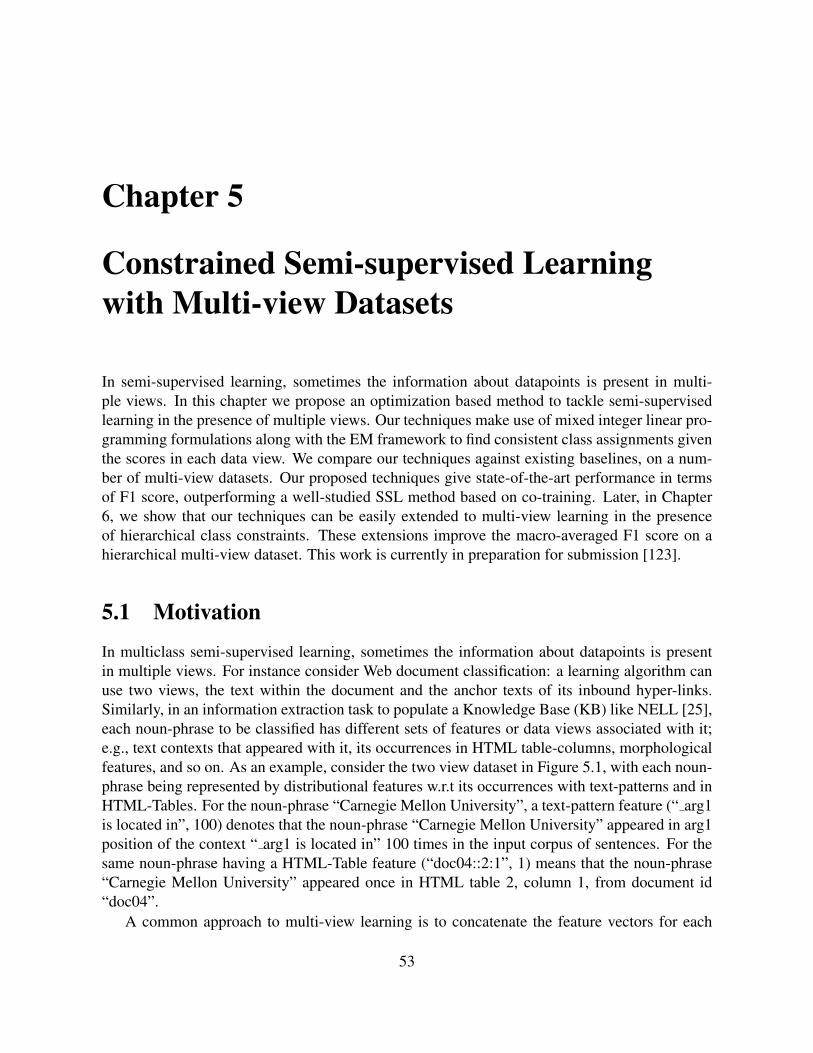
Chapter 5

Constrained Semi-supervised Learningwith Multi-view Datasets

In semi-supervised learning, sometimes the information about datapoints is present in multi-ple views. In this chapter we propose an optimization based method to tackle semi-supervisedlearning in the presence of multiple views. Our techniques make use of mixed integer linear pro-gramming formulations along with the EM framework to find consistent class assignments giventhe scores in each data view. We compare our techniques against existing baselines, on a num-ber of multi-view datasets. Our proposed techniques give state-of-the-art performance in termsof F1 score, outperforming a well-studied SSL method based on co-training. Later, in Chapter6, we show that our techniques can be easily extended to multi-view learning in the presenceof hierarchical class constraints. These extensions improve the macro-averaged F1 score on ahierarchical multi-view dataset. This work is currently in preparation for submission [123].

5.1 Motivation

In multiclass semi-supervised learning, sometimes the information about datapoints is presentin multiple views. For instance consider Web document classification: a learning algorithm canuse two views, the text within the document and the anchor texts of its inbound hyper-links.Similarly, in an information extraction task to populate a Knowledge Base (KB) like NELL [25],each noun-phrase to be classified has different sets of features or data views associated with it;e.g., text contexts that appeared with it, its occurrences in HTML table-columns, morphologicalfeatures, and so on. As an example, consider the two view dataset in Figure 5.1, with each noun-phrase being represented by distributional features w.r.t its occurrences with text-patterns and inHTML-Tables. For the noun-phrase “Carnegie Mellon University”, a text-pattern feature (“ arg1is located in”, 100) denotes that the noun-phrase “Carnegie Mellon University” appeared in arg1position of the context “ arg1 is located in” 100 times in the input corpus of sentences. For thesame noun-phrase having a HTML-Table feature (“doc04::2:1”, 1) means that the noun-phrase“Carnegie Mellon University” appeared once in HTML table 2, column 1, from document id“doc04”.

A common approach to multi-view learning is to concatenate the feature vectors for each

53

Figure 5.1: An example of multi-view dataset for Knowledge Base population task. For eachnoun-phrase distributional features are derived from two data sources. Occurrences of the noun-phrase with text-patterns result in View-1 and occurrences of the noun phrase in HTML tablecolumns result in View-2.

view but this is not always optimal. Multi-view learning [13, 97, 122, 131, 144] addresses thisproblem by introducing a different function to model each view, and jointly optimizing all thefunctions to exploit the redundant views and improve learning performance.

Multiple views are only one issue arising in complex real-world learning tasks. For instance,in the above mentioned KB population task, the labels assigned to each noun-phrase need tobe consistent with the hierarchical class constraints posed by the KB ontology. We deal withhierarchical multi-view learning problems in Chapter 6.

There has already been a lot of research in the individual areas of multi-view learning [13, 97,122, 131], semi-supervised learning [25, 98, 128], and learning in the presence of class hierar-chies [54, 67, 95, 127]. However, the problem of unifying these aspects into a single frameworkis less explored. In this chapter, we focus on the problem of multi-view semi-supervised learningand later extend it to incorporate class hierarchies in Chapter 6. We propose an optimizationbased formulation for this problem in the EM framework, which extends the popular K-Meansalgorithm. The main idea behind our approach is to use different binary labels to model mem-bership in each view. We then use mixed integer programming formulations to optimally assigna set of labels to each instance. Instead of collectively optimizing labels for all datapoints, wesolve an integer linear program for every datapoint, deciding the optimal label assignments forthe datapoint. We compare our methods against a state-of-the-art co-training approach, appliedto the semi-supervised spherical K-Means algorithm [10].

Our experiments show that our proposed methods work as well as or better than standardmulti-view baselines like multiplication (or addition) of scores, concatenation of feature vectors,and outperform a well-studied co-training based baseline, when applied in the standard multi-view k-way classification setting.

In Section 5.2 we propose our optimization framework for multi-view semi-supervised learn-ing. We then discuss various multi-view methods that can be instantiated using this framework.We then describe the datasets and experimental methodology in Section 5.3, and present ourfindings in Section 5.4. Finally, we discuss related work in Section 5.5, followed by conclusions.

54

5.2 Multi-View Semi-supervised LearningThe spherical K-Means algorithm [37], i.e., the K-Means algorithm with cosine similarity, is apopular method for clustering high-dimensional data such as text. In this section we will firstreview this existing algorithm, we then present our proposed extension called “multi-view spher-ical K-Means”. There are different ways in which scores from multiple views can be combinedto infer labels of every data point. We formulate the multi-view semi-supervised K-Means as ageneric optimization problem, and instantiate various existing methods, as well as our proposedmethods of combining scores from multiple views as special cases of this optimization problem.

5.2.1 Background and NotationLet us start with the spherical K-Means optimization problem, which makes use of cosine sim-ilarity between datapoint and centroids to do the clustering. In this algorithm [37], each docu-ment, as well as each cluster centroid, is represented as a high-dimensional unit-length vector.Let X = X1, . . . XN be the datapoints, C1, . . . CK be the clusters, yij be an indicator variablespecifying whether datapoint xj belongs to cluster Ci, and µi denotes the centroid for clusterCi. The task is to find optimal values of label assignments yij and cluster centroids µi, so as tooptimize the objective function given in Equation 5.1.

maxyij ,µi

(N∑j=1

K∑i=1

yij ∗ cos(xj, µi)

)s.t.

K∑i=1

yij = 1,∀j = 1 . . . N, yij ∈ 0, 1 (5.1)

Since the variables yij and µi are dependent on each other, the above function can be optimizedusing an iterative EM like algorithm such that the E step finds the best of values of yij givenµi’s and the M step takes these yij’s to recompute the optimal µi’s. Instead of probabilisticallyassigning a datapoint to a number of clusters, we choose hard assignments [28] i.e., we restrict yijas binary integers, hence this is the hard-EM algorithm. Fixing the values of µi’s, the objectivefunction is maximized when yij = 1 for i = argmaxi cos(xj, µi) and 0 otherwise. Let us nowcompute the µi that maximizes the objective given the values for yij’s. (〈a, b〉 denotes dot productof vectors a and b.)

maxµi

(N∑j=1

yij ∗ cos(xj, µi)

)= max

µi

⟨( N∑j=1

yijxj||xj||

),µi||µi||

⟩(5.2)

The Cauchy-Schwartz inequality [48] states that |〈x, y〉| ≤ ||x|| ∗ ||y||, and the two sides areequal only if x and y are linearly dependent. To maximize Equation 5.2, we can set µi =(∑

j yijxj||xj ||

). If we normalize xj and µi to be unit vectors, then the equations can be simplified

further. Given µi’s, yij = 1 for i = argmaxi⟨xj, µi

⟩and 0 otherwise. Similarly, given yij’s,

µi =∑

j yij ∗ xj . Henceforth, we assume that xj and µi are normalized to be unit vectors.Hence, cos(xj, µi) =

⟨xj, µi

⟩. Finally, the spherical K-Means algorithm repeats these two steps

iteratively till convergence.

55

5.2.2 Multi-View K-Means

We extend the spherical K-Means algorithm [37] for the multi-view setting and present a generaloptimization based framework for Multi-View K-Means. Later, we also describe various waysof combining evidence from the different views to instantiate multiple variants of this generalalgorithm.

In the multi-view scenario, a datapoint xj has a feature representation in each view denoted byx

(1)j in view 1 and x(2)

j in view 2. Once the datapoints are clustered in k clusters using K-Meansrepresentation, each centroid can also be represented differently in each view; i.e., centroid µican be represented as µ(1)

i in view 1 and µ(2)i in view 2. There is one score for every datapoint in

every view; i.e., we will have scores s(1)ij and s(2)

ij for datapoint xj and centroid µi in view 1 andview 2 respectively to be defined below. There is a single label assignment vector per datapointthat combines scores from different views, which we represent as matrix Y , i.e., yij = 1 indicatesthat datapoint xj belongs to cluster µi.

Let us define an effective score sij of datapoint xj belonging to cluster µi as an overall mea-sure of similarity of xj to µi under both views. Then the optimization problem described inEquation 5.1 can be re-written as:

maxyij

(N∑j=1

K∑i=1

yij ∗ sij

)s.t.

K∑i=1

yij = 1,∀j = 1 . . . N, yij ∈ 0, 1 (5.3)

In the multi-view scenario, the score sij can be defined as a function of s(1)ij and s(2)

ij . Thiscan be done in various ways: e.g., a linear combination of scores, multiplication of scores, takingmax or min over scores and so on.

Algorithm 9 describes a generic semi-supervised multi-view K-Means algorithm. It is differ-ent from standard K-Means in that each datapoint Xi and cluster centroid µj has a representationin each data view. In the E step of each EM iteration, for each unlabeled datapoint x we havea separate score from each view, a score of x belonging to a centroid µj . Line 8 in Algorithm9 combines these scores and decides best cluster assignment for each datapoint. In the M step,centroids are recomputed per view based on the label assignments done in the E step. For sim-plicity of understanding, the algorithm is presented for two data views. However our techniquesare easily applicable to datasets with more than two views.

Next, we will see various ways in which the cluster assignment step (line 8) and the cen-troid computation step (line 10) in this algorithm can be done, leading to new multi-view SSLalgorithms. Recall that instead of probabilistically assigning a datapoint to a number of clusters,we choose hard assignments, i.e., we restrict Y u

t (x) (in Line 8) as binary integers, hence this isthe hard-EM algorithm (or classification EM) [28]. Even though finding an optimal set of hardassignments using mixed integer programs is relatively more expensive than soft assignments,we are solving it per datapoint, instead of collectively optimizing labels for all datapoints. Hencewe can divide the datapoints into multiple shards and parallelize the computation in Line 8 ofAlgorithm 9. Since we are using the spherical K-Means algorithm in a semi-supervised setting,henceforth we will use “cluster” and class” interchangeably.

56

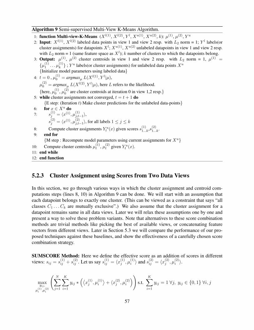
Algorithm 9 Semi-supervised Multi-View K-Means Algorithm.1: function Multi-view-K-Means (X l(1), X l(2), Y l, Xu(1), Xu(2), k): µ(1), µ(2), Y u

2: Input: X l(1), X l(2) labeled data points in view 1 and view 2 resp. with L2 norm = 1; Y l labels(orcluster assignments) for datapoints X l; Xu(1), Xu(2) unlabeled datapoints in view 1 and view 2 resp.with L2 norm = 1 (same feature space as X l); k number of clusters to which the datapoints belong.

3: Output: µ(1), µ(2) cluster centroids in view 1 and view 2 resp. with L2 norm = 1, µ(1) =

µ(1)1 . . . µ

(1)k ; Y u labels(or cluster assignments) for unlabeled data points Xu

Initialize model parameters using labeled data4: t = 0 , µ(1)

0 = argmaxµ L(Xl(1), Y l|µ),

µ(2)0 = argmaxµ L(X

l(2), Y l|µ), here L refers to the likelihood.

here, µ(1)0 , µ(2)

0 are cluster centroids at iteration 0 in view 1,2 resp.5: while cluster assignments not converged, t = t+ 1 do

E step: (Iteration t) Make cluster predictions for the unlabeled data-points6: for x ∈ Xu do7: s

(1)j = 〈x(1), µ

(1)j,t−1〉,

s(2)j = 〈x(1), µ

(2)j,t−1〉, for all labels 1 ≤ j ≤ k

8: Compute cluster assignments Y ut (x) given scores s(1)

1...k,s(2)1...k.

9: end forM step : Recompute model parameters using current assignments for Xu

10: Compute cluster centroids µ(1)t , µ(2)

t given Y ut (x).

11: end while12: end function

5.2.3 Cluster Assignment using Scores from Two Data Views

In this section, we go through various ways in which the cluster assignment and centroid com-putations steps (lines 8, 10) in Algorithm 9 can be done. We will start with an assumption thateach datapoint belongs to exactly one cluster. (This can be viewed as a constraint that says “allclasses C1 . . . Ck are mutually exclusive”.) We also assume that the cluster assignment for adatapoint remains same in all data views. Later we will relax these assumptions one by one andpresent a way to solve these problem variants. Note that alternatives to these score combinationmethods are trivial methods like picking the best of available views, or concatenating featurevectors from different views. Later in Section 5.3 we will compare the performance of our pro-posed techniques against these baselines, and show the effectiveness of a carefully chosen scorecombination strategy.

SUMSCORE Method: Here we define the effective score as an addition of scores in differentviews: sij = s

(1)ij + s

(2)ij . Let us say s(1)

ij = 〈x(1)j , µ

(1)i 〉 and s(2)

ij = 〈x(2)j , µ

(2)i 〉.

maxyij ,

µ(1)i ,µ

(2)i

(N∑j=1

K∑i=1

yij ∗(⟨x

(1)j , µ

(1)i

⟩+ 〈x(2)

j , µ(2)i

))s.t.

K∑i=1

yij = 1 ∀j, yij ∈ 0, 1 ∀i, j

57

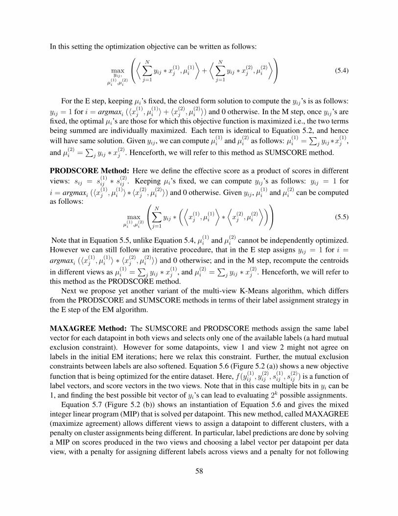
In this setting the optimization objective can be written as follows:

maxyij ,

µ(1)i ,µ

(2)i

⟨ N∑j=1

yij ∗ x(1)j , µ

(1)i

⟩+

⟨ N∑j=1

yij ∗ x(2)j , µ

(2)i

⟩ (5.4)

For the E step, keeping µi’s fixed, the closed form solution to compute the yij’s is as follows:yij = 1 for i = argmaxi (〈x(1)

j , µ(1)i 〉+ 〈x

(2)j , µ

(2)i 〉) and 0 otherwise. In the M step, once yij’s are

fixed, the optimal µi’s are those for which this objective function is maximized i.e., the two termsbeing summed are individually maximized. Each term is identical to Equation 5.2, and hencewill have same solution. Given yij , we can compute µ(1)

i and µ(2)i as follows: µ(1)

i =∑

j yij ∗x(1)j ,

and µ(2)i =

∑j yij ∗ x

(2)j . Henceforth, we will refer to this method as SUMSCORE method.

PRODSCORE Method: Here we define the effective score as a product of scores in differentviews: sij = s

(1)ij ∗ s

(2)ij . Keeping µi’s fixed, we can compute yij’s as follows: yij = 1 for

i = argmaxi (〈x(1)j , µ

(1)i 〉∗ 〈x

(2)j , µ

(2)i 〉) and 0 otherwise. Given yij , µ

(1)i and µ(2)

i can be computedas follows:

maxµ(1)i ,µ

(2)i

N∑j=1

yij ∗(⟨

x(1)j , µ

(1)i

⟩∗⟨x

(2)j , µ

(2)i

⟩) (5.5)

Note that in Equation 5.5, unlike Equation 5.4, µ(1)i and µ(2)

i cannot be independently optimized.However we can still follow an iterative procedure, that in the E step assigns yij = 1 for i =

argmaxi (〈x(1)j , µ

(1)i 〉 ∗ 〈x

(2)j , µ

(2)i 〉) and 0 otherwise; and in the M step, recompute the centroids

in different views as µ(1)i =

∑j yij ∗ x

(1)j , and µ(2)

i =∑

j yij ∗ x(2)j . Henceforth, we will refer to

this method as the PRODSCORE method.Next we propose yet another variant of the multi-view K-Means algorithm, which differs

from the PRODSCORE and SUMSCORE methods in terms of their label assignment strategy inthe E step of the EM algorithm.

MAXAGREE Method: The SUMSCORE and PRODSCORE methods assign the same labelvector for each datapoint in both views and selects only one of the available labels (a hard mutualexclusion constraint). However for some datapoints, view 1 and view 2 might not agree onlabels in the initial EM iterations; here we relax this constraint. Further, the mutual exclusionconstraints between labels are also softened. Equation 5.6 (Figure 5.2 (a)) shows a new objectivefunction that is being optimized for the entire dataset. Here, f(y

(1)ij , y

(2)ij , s

(1)ij , s

(2)ij ) is a function of

label vectors, and score vectors in the two views. Note that in this case multiple bits in yi can be1, and finding the best possible bit vector of yi’s can lead to evaluating 2k possible assignments.

Equation 5.7 (Figure 5.2 (b)) shows an instantiation of Equation 5.6 and gives the mixedinteger linear program (MIP) that is solved per datapoint. This new method, called MAXAGREE(maximize agreement) allows different views to assign a datapoint to different clusters, with apenalty on cluster assignments being different. In particular, label predictions are done by solvinga MIP on scores produced in the two views and choosing a label vector per datapoint per dataview, with a penalty for assigning different labels across views and a penalty for not following

58

(a)maximize

y(1)ij ,y

(2)ij ,µ

(1)i ,µ

(2)i

(∑j

(f(y

(1)ij , y

(2)ij , s

(1)ij , s

(2)ij )−

(Penalty for

( K∑i=1

y(1)ij 6= y

(2)ij

),( 2∑v=1

K∑i=1

y(v)ij 6= 1

))))subject to, y

(1)ij ∈ 0, 1, y

(2)ij ∈ 0, 1

(5.6)

(b)

maximizey(1)i ,y

(2)i ,di,ζ1,ζ2,δ1,δ2

(α1 ∗

(∑i

y(1)i ∗ s

(1)i + y

(2)i ∗ s

(2)i

)− α2 ∗

(∑i

di

)− α3 ∗

(ζ1 + ζ2 + δ1 + δ2

))subject to, di = |y(1)

i − y(2)i |, ∀i = 1 . . . k∑

i

y(1)i ≤ 1 + δ1,

∑i

y(2)i ≤ 1 + δ2, ∀i = 1 . . . k∑

i

y(1)i ≥ 1− ζ1,

∑i

y(2)i ≥ 1− ζ2, ∀i = 1 . . . k

ζ1, ζ2, δ1, δ2 ≥ 0, y(1)i ∈ 0, 1, y

(2)i ∈ 0, 1 ∀i

(5.7)Figure 5.2: (a) Optimization formulation for multi-view learning (b) Mixed integer program forMAXAGREE method with two views.

the mutual exclusion constraints. Further, Equation 5.6 can be independently optimized for eachdatapoint.

For each datapoint s(1)i and s(2)

i are scores of x belonging to cluster i according to data view1 and view 2 respectively. y(1)

i and y(2)i represent cluster assignments in view 1 and view 2 re-

spectively. The term di is the penalty on y(1)i and y(2)

i being different. Terms ζ1 and ζ2 are thepenalty terms for the constraint that each datapoint should be assigned to at least one cluster ineach view. Similarly, δ1 and δ2 are the penalty terms for the constraint that each datapoint shouldbe assigned to at most one cluster in each view. Terms α1, α2 and α3 are constants that definerelative importance of terms in the objective function.

COTRAIN Method: We also experiment with a well-studied co-training based method CO-TRAIN as one of the baselines. This method is a multi-view spherical K-Means algorithm thatis proposed by Bickel and Scheffer [10]. In particular, it is a co-training variant of the sphericalK-Means algorithm, in which predictions made for view 1 in the E step are used to recomputecentroids of view 2 in the M step and visa versa.

5.3 Datasets and Experimental MethodologyHere, we first describe the datasets used. We then explain the experimental setup and evaluationcriteria used.

5.3.1 DatasetsWe present experiments with eight multi-view datasets, summarized in Table 5.1. The first sixof them are publicly available, and the last two were created by us for exploring the multi-view learning task. Cora, WebKB and CiteSeer1 [52] consists of two data views for scientificpublications. The first view consists of 0/1-valued word vector derived from the document text,and the other view is citation links between these documents (represented as binary features).

59

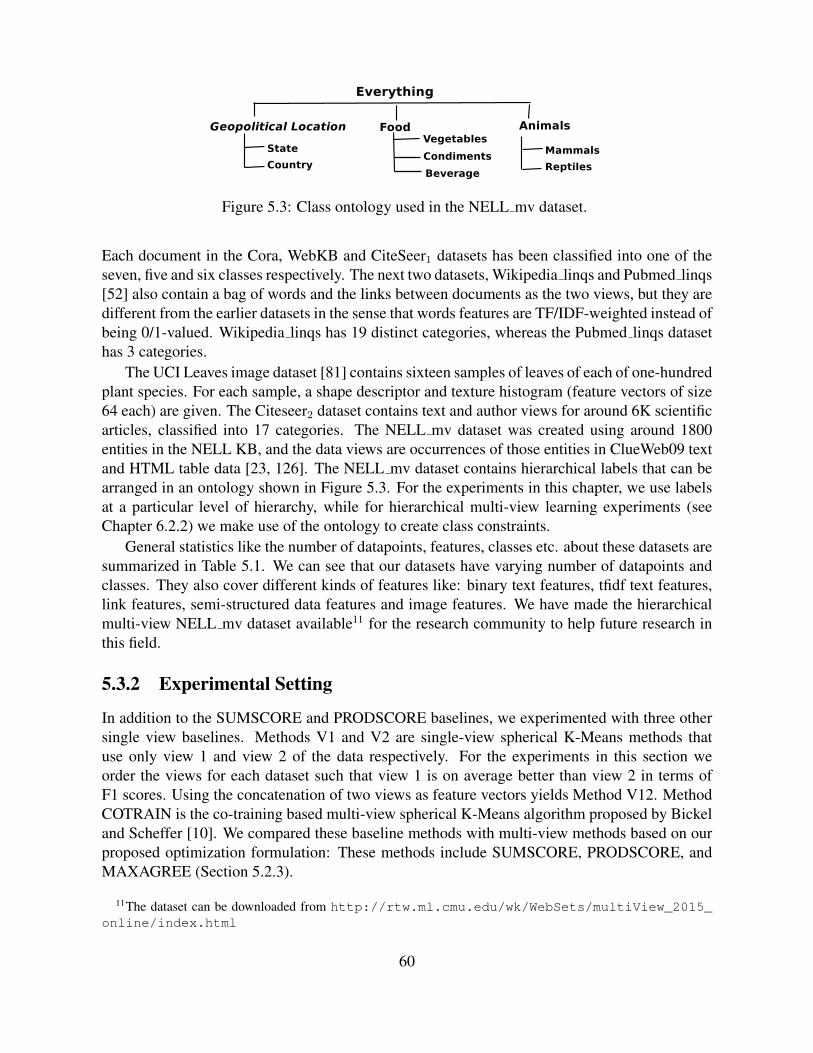
Figure 5.3: Class ontology used in the NELL mv dataset.

Each document in the Cora, WebKB and CiteSeer1 datasets has been classified into one of theseven, five and six classes respectively. The next two datasets, Wikipedia linqs and Pubmed linqs[52] also contain a bag of words and the links between documents as the two views, but they aredifferent from the earlier datasets in the sense that words features are TF/IDF-weighted instead ofbeing 0/1-valued. Wikipedia linqs has 19 distinct categories, whereas the Pubmed linqs datasethas 3 categories.

The UCI Leaves image dataset [81] contains sixteen samples of leaves of each of one-hundredplant species. For each sample, a shape descriptor and texture histogram (feature vectors of size64 each) are given. The Citeseer2 dataset contains text and author views for around 6K scientificarticles, classified into 17 categories. The NELL mv dataset was created using around 1800entities in the NELL KB, and the data views are occurrences of those entities in ClueWeb09 textand HTML table data [23, 126]. The NELL mv dataset contains hierarchical labels that can bearranged in an ontology shown in Figure 5.3. For the experiments in this chapter, we use labelsat a particular level of hierarchy, while for hierarchical multi-view learning experiments (seeChapter 6.2.2) we make use of the ontology to create class constraints.

General statistics like the number of datapoints, features, classes etc. about these datasets aresummarized in Table 5.1. We can see that our datasets have varying number of datapoints andclasses. They also cover different kinds of features like: binary text features, tfidf text features,link features, semi-structured data features and image features. We have made the hierarchicalmulti-view NELL mv dataset available11 for the research community to help future research inthis field.

5.3.2 Experimental Setting

In addition to the SUMSCORE and PRODSCORE baselines, we experimented with three othersingle view baselines. Methods V1 and V2 are single-view spherical K-Means methods thatuse only view 1 and view 2 of the data respectively. For the experiments in this section weorder the views for each dataset such that view 1 is on average better than view 2 in terms ofF1 scores. Using the concatenation of two views as feature vectors yields Method V12. MethodCOTRAIN is the co-training based multi-view spherical K-Means algorithm proposed by Bickeland Scheffer [10]. We compared these baseline methods with multi-view methods based on ourproposed optimization formulation: These methods include SUMSCORE, PRODSCORE, andMAXAGREE (Section 5.2.3).

11The dataset can be downloaded from http://rtw.ml.cmu.edu/wk/WebSets/multiView_2015_online/index.html

60

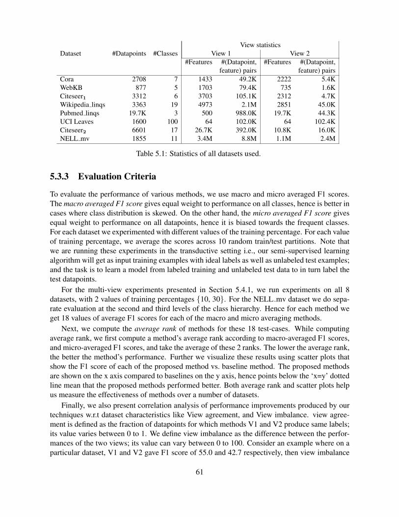
View statisticsDataset #Datapoints #Classes View 1 View 2

#Features #(Datapoint, #Features #(Datapoint,feature) pairs feature) pairs

Cora 2708 7 1433 49.2K 2222 5.4KWebKB 877 5 1703 79.4K 735 1.6KCiteseer1 3312 6 3703 105.1K 2312 4.7KWikipedia linqs 3363 19 4973 2.1M 2851 45.0KPubmed linqs 19.7K 3 500 988.0K 19.7K 44.3KUCI Leaves 1600 100 64 102.0K 64 102.4KCiteseer2 6601 17 26.7K 392.0K 10.8K 16.0KNELL mv 1855 11 3.4M 8.8M 1.1M 2.4M

Table 5.1: Statistics of all datasets used.

5.3.3 Evaluation Criteria

To evaluate the performance of various methods, we use macro and micro averaged F1 scores.The macro averaged F1 score gives equal weight to performance on all classes, hence is better incases where class distribution is skewed. On the other hand, the micro averaged F1 score givesequal weight to performance on all datapoints, hence it is biased towards the frequent classes.For each dataset we experimented with different values of the training percentage. For each valueof training percentage, we average the scores across 10 random train/test partitions. Note thatwe are running these experiments in the transductive setting i.e., our semi-supervised learningalgorithm will get as input training examples with ideal labels as well as unlabeled test examples;and the task is to learn a model from labeled training and unlabeled test data to in turn label thetest datapoints.

For the multi-view experiments presented in Section 5.4.1, we run experiments on all 8datasets, with 2 values of training percentages 10, 30. For the NELL mv dataset we do sepa-rate evaluation at the second and third levels of the class hierarchy. Hence for each method weget 18 values of average F1 scores for each of the macro and micro averaging methods.

Next, we compute the average rank of methods for these 18 test-cases. While computingaverage rank, we first compute a method’s average rank according to macro-averaged F1 scores,and micro-averaged F1 scores, and take the average of these 2 ranks. The lower the average rank,the better the method’s performance. Further we visualize these results using scatter plots thatshow the F1 score of each of the proposed method vs. baseline method. The proposed methodsare shown on the x axis compared to baselines on the y axis, hence points below the ‘x=y’ dottedline mean that the proposed methods performed better. Both average rank and scatter plots helpus measure the effectiveness of methods over a number of datasets.

Finally, we also present correlation analysis of performance improvements produced by ourtechniques w.r.t dataset characteristics like View agreement, and View imbalance. view agree-ment is defined as the fraction of datapoints for which methods V1 and V2 produce same labels;its value varies between 0 to 1. We define view imbalance as the difference between the perfor-mances of the two views; its value can vary between 0 to 100. Consider an example where on aparticular dataset, V1 and V2 gave F1 score of 55.0 and 42.7 respectively, then view imbalance

61

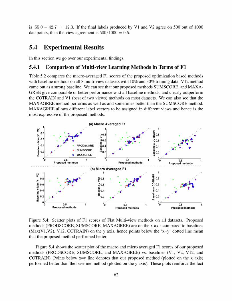
is |55.0 − 42.7| = 12.3. If the final labels produced by V1 and V2 agree on 500 out of 1000datapoints, then the view agreement is 500/1000 = 0.5.

5.4 Experimental ResultsIn this section we go over our experimental findings.

5.4.1 Comparison of Multi-view Learning Methods in Terms of F1Table 5.2 compares the macro-averaged F1 scores of the proposed optimization based methodswith baseline methods on all 8 multi-view datasets with 10% and 30% training data. V12 methodcame out as a strong baseline. We can see that our proposed methods SUMSCORE, and MAXA-GREE give comparable or better performance w.r.t all baseline methods, and clearly outperformthe COTRAIN and V1 (best of two views) methods on most datasets. We can also see that theMAXAGREE method performs as well as and sometimes better than the SUMSCORE method.MAXAGREE allows different label vectors to be assigned in different views and hence is themost expressive of the proposed methods.

0 0.5 10

0.2

0.4

0.6

0.8

1

Baselin

e =

Max(V

1, V

2)

Proposed methods

0 0.5 10

0.2

0.4

0.6

0.8

1

Baselin

e =

Max(V

1, V

2)

Proposed methods

0 0.5 10

0.2

0.4

0.6

0.8

1

Baselin

e =

V12

Proposed methods

0 0.5 10

0.2

0.4

0.6

0.8

1

Baselin

e =

V12

Proposed methods

0 0.5 10

0.2

0.4

0.6

0.8

1

Baselin

e =

CO

TR

AIN

Proposed methods

0 0.5 10

0.2

0.4

0.6

0.8

1

Baselin

e =

CO

TR

AIN

Proposed methods

PRODSCORE

SUMSCORE

MAXAGREE

(a) Macro Averaged F1

(b) Micro Averaged F1

Figure 5.4: Scatter plots of F1 scores of Flat Multi-view methods on all datasets. Proposedmethods (PRODSCORE, SUMSCORE, MAXAGREE) are on the x axis compared to baselines(Max(V1,V2), V12, COTRAIN) on the y axis, hence points below the ‘x=y’ dotted line meanthat the proposed method performed better.

Figure 5.4 shows the scatter plot of the macro and micro averaged F1 scores of our proposedmethods (PRODSCORE, SUMSCORE, and MAXAGREE) vs. baselines (V1, V2, V12, andCOTRAIN). Points below x=y line denotes that our proposed method (plotted on the x axis)performed better than the baseline method (plotted on the y axis). These plots reinforce the fact

62

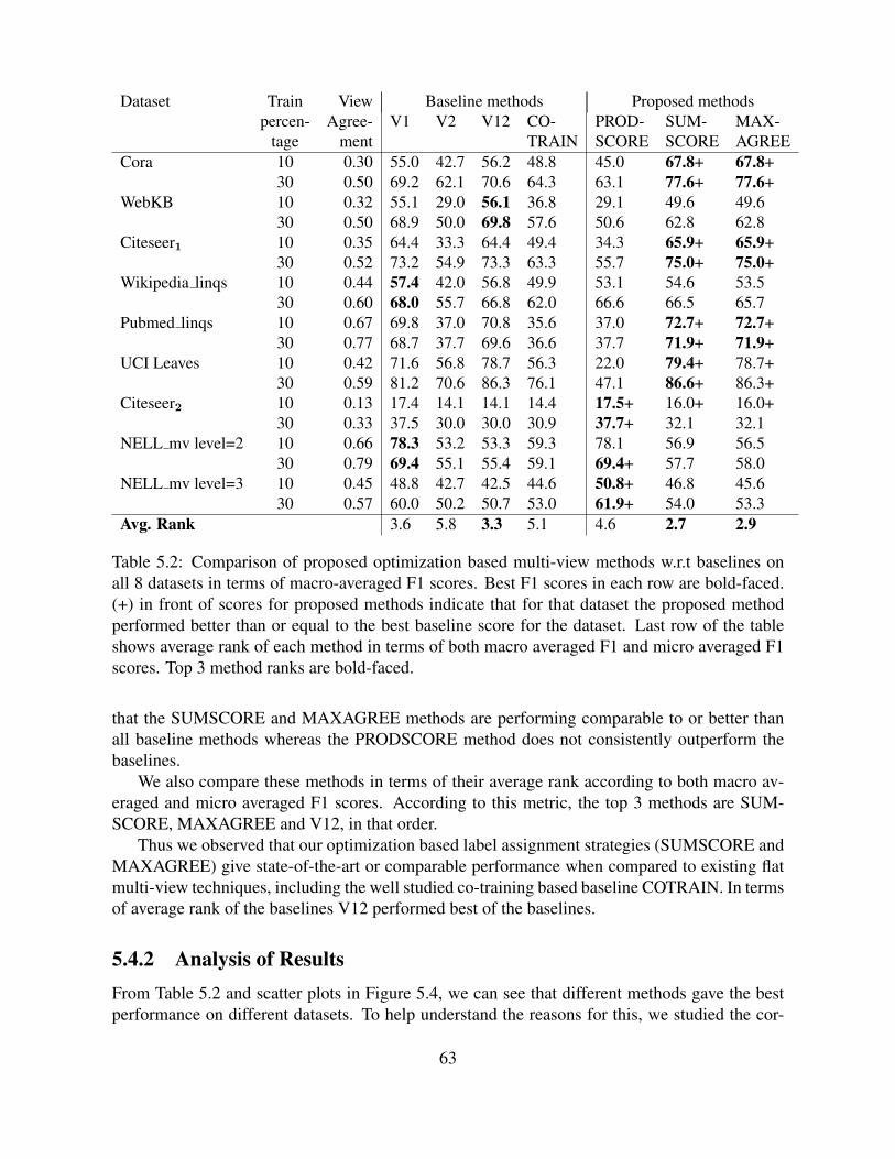
Dataset Train View Baseline methods Proposed methodspercen- Agree- V1 V2 V12 CO- PROD- SUM- MAX-

tage ment TRAIN SCORE SCORE AGREECora 10 0.30 55.0 42.7 56.2 48.8 45.0 67.8+ 67.8+

30 0.50 69.2 62.1 70.6 64.3 63.1 77.6+ 77.6+WebKB 10 0.32 55.1 29.0 56.1 36.8 29.1 49.6 49.6

30 0.50 68.9 50.0 69.8 57.6 50.6 62.8 62.8Citeseer1 10 0.35 64.4 33.3 64.4 49.4 34.3 65.9+ 65.9+

30 0.52 73.2 54.9 73.3 63.3 55.7 75.0+ 75.0+Wikipedia linqs 10 0.44 57.4 42.0 56.8 49.9 53.1 54.6 53.5

30 0.60 68.0 55.7 66.8 62.0 66.6 66.5 65.7Pubmed linqs 10 0.67 69.8 37.0 70.8 35.6 37.0 72.7+ 72.7+

30 0.77 68.7 37.7 69.6 36.6 37.7 71.9+ 71.9+UCI Leaves 10 0.42 71.6 56.8 78.7 56.3 22.0 79.4+ 78.7+

30 0.59 81.2 70.6 86.3 76.1 47.1 86.6+ 86.3+Citeseer2 10 0.13 17.4 14.1 14.1 14.4 17.5+ 16.0+ 16.0+

30 0.33 37.5 30.0 30.0 30.9 37.7+ 32.1 32.1NELL mv level=2 10 0.66 78.3 53.2 53.3 59.3 78.1 56.9 56.5

30 0.79 69.4 55.1 55.4 59.1 69.4+ 57.7 58.0NELL mv level=3 10 0.45 48.8 42.7 42.5 44.6 50.8+ 46.8 45.6

30 0.57 60.0 50.2 50.7 53.0 61.9+ 54.0 53.3Avg. Rank 3.6 5.8 3.3 5.1 4.6 2.7 2.9

Table 5.2: Comparison of proposed optimization based multi-view methods w.r.t baselines onall 8 datasets in terms of macro-averaged F1 scores. Best F1 scores in each row are bold-faced.(+) in front of scores for proposed methods indicate that for that dataset the proposed methodperformed better than or equal to the best baseline score for the dataset. Last row of the tableshows average rank of each method in terms of both macro averaged F1 and micro averaged F1scores. Top 3 method ranks are bold-faced.

that the SUMSCORE and MAXAGREE methods are performing comparable to or better thanall baseline methods whereas the PRODSCORE method does not consistently outperform thebaselines.

We also compare these methods in terms of their average rank according to both macro av-eraged and micro averaged F1 scores. According to this metric, the top 3 methods are SUM-SCORE, MAXAGREE and V12, in that order.

Thus we observed that our optimization based label assignment strategies (SUMSCORE andMAXAGREE) give state-of-the-art or comparable performance when compared to existing flatmulti-view techniques, including the well studied co-training based baseline COTRAIN. In termsof average rank of the baselines V12 performed best of the baselines.

5.4.2 Analysis of ResultsFrom Table 5.2 and scatter plots in Figure 5.4, we can see that different methods gave the bestperformance on different datasets. To help understand the reasons for this, we studied the cor-

63

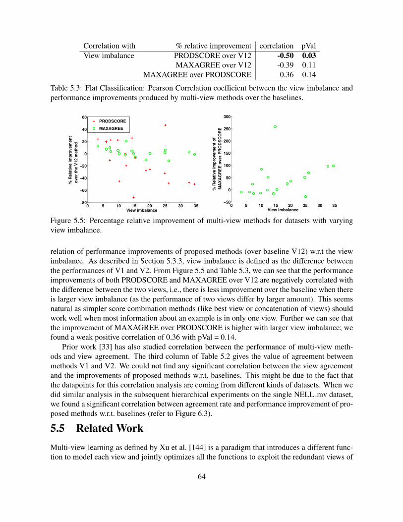
Correlation with % relative improvement correlation pValView imbalance PRODSCORE over V12 -0.50 0.03

MAXAGREE over V12 -0.39 0.11MAXAGREE over PRODSCORE 0.36 0.14

Table 5.3: Flat Classification: Pearson Correlation coefficient between the view imbalance andperformance improvements produced by multi-view methods over the baselines.

0 5 10 15 20 25 30 35−80

−60

−40

−20

0

20

40

60

View imbalance

% R

ela

tive im

pro

vem

en

t

over

the V

12 m

eth

od

PRODSCORE

MAXAGREE

0 5 10 15 20 25 30 35−50

0

50

100

150

200

250

300

View imbalance%

Rela

tive im

pro

vem

en

t o

f

MA

XA

GR

EE

over

PR

OD

SC

OR

EFigure 5.5: Percentage relative improvement of multi-view methods for datasets with varyingview imbalance.

relation of performance improvements of proposed methods (over baseline V12) w.r.t the viewimbalance. As described in Section 5.3.3, view imbalance is defined as the difference betweenthe performances of V1 and V2. From Figure 5.5 and Table 5.3, we can see that the performanceimprovements of both PRODSCORE and MAXAGREE over V12 are negatively correlated withthe difference between the two views, i.e., there is less improvement over the baseline when thereis larger view imbalance (as the performance of two views differ by larger amount). This seemsnatural as simpler score combination methods (like best view or concatenation of views) shouldwork well when most information about an example is in only one view. Further we can see thatthe improvement of MAXAGREE over PRODSCORE is higher with larger view imbalance; wefound a weak positive correlation of 0.36 with pVal = 0.14.

Prior work [33] has also studied correlation between the performance of multi-view meth-ods and view agreement. The third column of Table 5.2 gives the value of agreement betweenmethods V1 and V2. We could not find any significant correlation between the view agreementand the improvements of proposed methods w.r.t. baselines. This might be due to the fact thatthe datapoints for this correlation analysis are coming from different kinds of datasets. When wedid similar analysis in the subsequent hierarchical experiments on the single NELL mv dataset,we found a significant correlation between agreement rate and performance improvement of pro-posed methods w.r.t. baselines (refer to Figure 6.3).

5.5 Related WorkMulti-view learning as defined by Xu et al. [144] is a paradigm that introduces a different func-tion to model each view and jointly optimizes all the functions to exploit the redundant views of

64

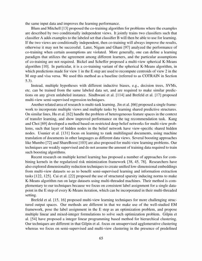
the same input data and improves the learning performance.Blum and Mitchell [13] proposed the co-training algorithm for problems where the examples

are described by two conditionally independent views. It jointly trains two classifiers such thatclassifier A adds examples to the labeled set that classifier B will then be able to use for learning.If the two views are conditionally independent, then co-training will always improve the results,otherwise it may not be successful. Later, Nigam and Ghani [97] analyzed the performance ofco-training when certain assumptions are violated. More generally, one can define a learningparadigm that utilizes the agreement among different learners, and the particular assumptionsof co-training are not required. Bickel and Scheffer proposed a multi-view spherical K-Meansalgorithm [10]. In particular, it is a co-training variant of the spherical K-Means algorithm, inwhich predictions made for view 1 in the E step are used to recompute centroids of view 2 in theM step and visa versa. We used this method as a baseline (referred to as COTRAIN in Section5.3).

Instead, multiple hypotheses with different inductive biases, e.g., decision trees, SVMs,etc. can be trained from the same labeled data set, and are required to make similar predic-tions on any given unlabeled instance. Sindhwani et al. [114] and Brefeld et al. [17] proposedmulti-view semi-supervised regression techniques.

Another related area of research is multi-task learning. Jin et al. [66] proposed a single frame-work to incorporate multiple views and multiple tasks by learning shared predictive structures.On similar lines, Hu et al. [62] handle the problem of heterogeneous feature spaces in the contextof transfer learning, and show improved performance on the tag recommendation task. Kangand Choi [69] developed a method based on restricted deep belief networks for multi-view prob-lems, such that layer of hidden nodes in the belief network have view-specific shared hiddennodes. Usunier et al. [131] focus on learning to rank multilingual documents, using machinetranslation of documents in other languages as different data views. Several boosting approacheslike Mumbo [72] and ShareBoost [103] are also proposed for multi-view learning problems. Ourtechniques are weakly supervised and do not assume the amount of training data required to trainsuch boosting algorithms.

Recent research on multiple kernel learning has proposed a number of approaches for com-bining kernels in the regularized risk minimization framework [38, 45, 78]. Researchers havealso explored dimensionality reduction techniques to create unified low-dimensional embeddingsfrom multi-view datasets so as to benefit semi-supervised learning and information extractiontasks [122, 125]. Cai et al. [22] proposed the use of structured sparsity inducing norms to makeK-Means algorithm run on large datasets using multi-threaded machines. Their method is com-plementary to our techniques because we focus on consistent label assignment for a single data-point in the E step of every K-Means iteration, which can be incorporated in their multi-threadedsetting.

Brefeld et al. [15, 16] proposed multi-view learning techniques for more challenging struc-tured output spaces. Our methods are different in that we make use of the well-studied EMframework, pose the label assignment in the E step as an optimization problem, and proposemultiple linear and mixed-integer formulations to solve such optimization problem. Gilpin etal. [54] have proposed a integer linear programming based method for hierarchical clustering.Our techniques are different in that Gilpin et al. focus on unsupervised agglomerative clusteringwhereas we focus on semi-supervised and multi-view clustering in the presence of predefined

65

class hierarchy.

5.6 ConclusionsIn this chapter, we investigated the problem of semi-supervised learning in the presence ofmultiple-data views. We formulated the problem as an optimization problem, and solved it usingthe standard EM framework. We then focused on the sub-problem of assigning labels to each dat-apoint (part of E step), and studied various methods for such prediction. Our proposed methodsolves a mixed integer linear program to find consistent class assignments given the scores ineach data view. Because our multi-view techniques are broadly similar to co-training based al-gorithms, we also compared them to a seeded version of multi-view spherical K-Means algorithmthat is proposed by Bickel and Scheffer [10]. Our methods produced better performance in termsof macro-averaged F1 score compared to this co-training baseline.

We present extensive experiments on 8 different multi-view datasets, including documentclassification, image classification, publication categorization and knowledge based informationextraction datasets. The data views also vary in their nature including word occurrences, binaryfeatures, link features, image histograms and co-occurrence features. We showed that our tech-niques give state-of-the-art performance when compared to existing multi-view learning methodsincluding the co-training based algorithm proposed by Bickel and Scheffer [10], on the problemof flat multi-view semi-supervised learning.

Finally, we have made the hierarchical multi-view NELL mv dataset available12. We havepublished the text context and HTML table features, class hierarchy, hierarchical labels for allentities, and seed train-test partitions of NELL mv dataset used in this thesis.

12Dataset link: http://rtw.ml.cmu.edu/wk/WebSets/multiView_2015_online

66

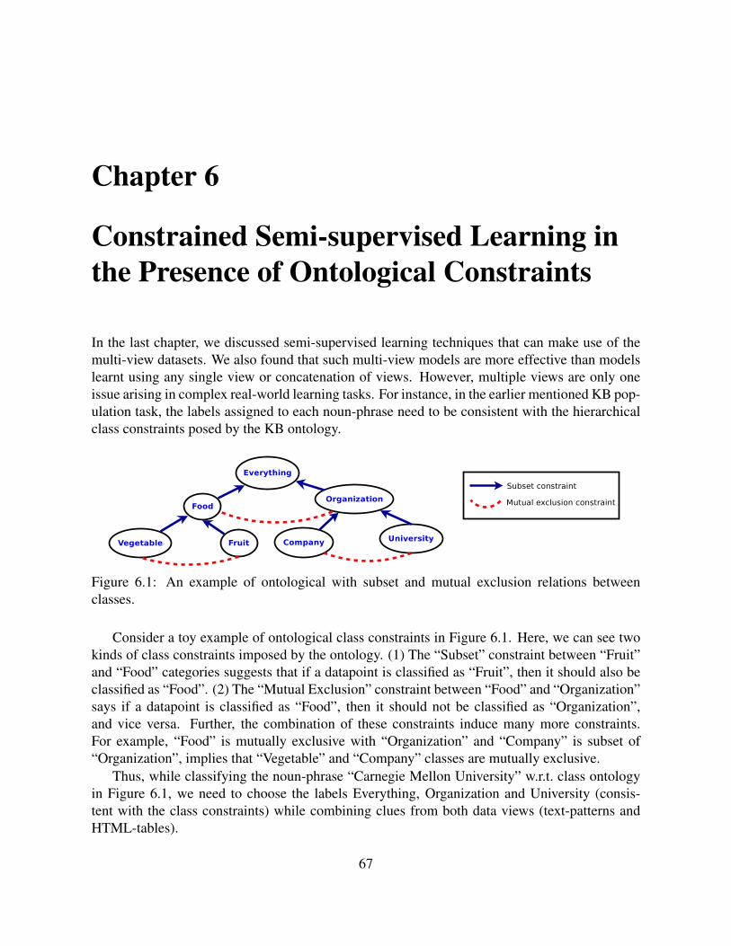
Chapter 6

Constrained Semi-supervised Learning inthe Presence of Ontological Constraints

In the last chapter, we discussed semi-supervised learning techniques that can make use of themulti-view datasets. We also found that such multi-view models are more effective than modelslearnt using any single view or concatenation of views. However, multiple views are only oneissue arising in complex real-world learning tasks. For instance, in the earlier mentioned KB pop-ulation task, the labels assigned to each noun-phrase need to be consistent with the hierarchicalclass constraints posed by the KB ontology.

Figure 6.1: An example of ontological with subset and mutual exclusion relations betweenclasses.

Consider a toy example of ontological class constraints in Figure 6.1. Here, we can see twokinds of class constraints imposed by the ontology. (1) The “Subset” constraint between “Fruit”and “Food” categories suggests that if a datapoint is classified as “Fruit”, then it should also beclassified as “Food”. (2) The “Mutual Exclusion” constraint between “Food” and “Organization”says if a datapoint is classified as “Food”, then it should not be classified as “Organization”,and vice versa. Further, the combination of these constraints induce many more constraints.For example, “Food” is mutually exclusive with “Organization” and “Company” is subset of“Organization”, implies that “Vegetable” and “Company” classes are mutually exclusive.

Thus, while classifying the noun-phrase “Carnegie Mellon University” w.r.t. class ontologyin Figure 6.1, we need to choose the labels Everything, Organization and University (consis-tent with the class constraints) while combining clues from both data views (text-patterns andHTML-tables).

67

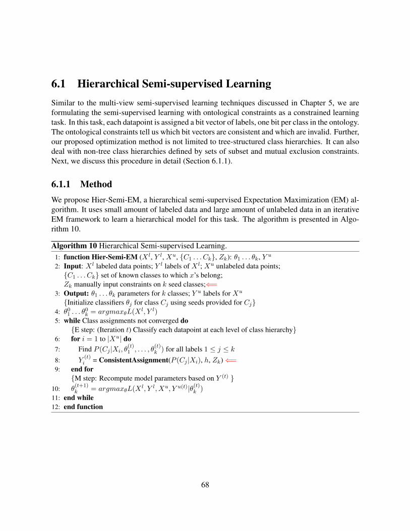
6.1 Hierarchical Semi-supervised LearningSimilar to the multi-view semi-supervised learning techniques discussed in Chapter 5, we areformulating the semi-supervised learning with ontological constraints as a constrained learningtask. In this task, each datapoint is assigned a bit vector of labels, one bit per class in the ontology.The ontological constraints tell us which bit vectors are consistent and which are invalid. Further,our proposed optimization method is not limited to tree-structured class hierarchies. It can alsodeal with non-tree class hierarchies defined by sets of subset and mutual exclusion constraints.Next, we discuss this procedure in detail (Section 6.1.1).

6.1.1 MethodWe propose Hier-Semi-EM, a hierarchical semi-supervised Expectation Maximization (EM) al-gorithm. It uses small amount of labeled data and large amount of unlabeled data in an iterativeEM framework to learn a hierarchical model for this task. The algorithm is presented in Algo-rithm 10.

Algorithm 10 Hierarchical Semi-supervised Learning.1: function Hier-Semi-EM (X l, Y l, Xu, C1 . . . Ck, Zk): θ1 . . . θk, Y u

2: Input: X l labeled data points; Y l labels of X l; Xu unlabeled data points;C1 . . . Ck set of known classes to which x’s belong;Zk manually input constraints on k seed classes;⇐=

3: Output: θ1 . . . θk parameters for k classes; Y u labels for Xu

Initialize classifiers θj for class Cj using seeds provided for Cj4: θ0

1 . . . θ0k = argmaxθL(X

l, Y l)5: while Class assignments not converged do

E step: (Iteration t) Classify each datapoint at each level of class hierarchy6: for i = 1 to |Xu| do7: Find P (Cj |Xi, θ

(t)1 , . . . , θ

(t)k ) for all labels 1 ≤ j ≤ k

8: Y(t)i = ConsistentAssignment(P (Cj |Xi), h, Zk)⇐=

9: end forM step: Recompute model parameters based on Y (t)

10: θ(t+1)k = argmaxθL(X

l, Y l, Xu, Y u(t)|θ(t)k )

11: end while12: end function

68

Before getting into the details of the algorithm, let us review the notations. Let X =X1, . . . XN be the datapoints to be classified, and C1, . . . CK be the KB categories. Letyji ∈ 0, 1 be an indicator variable specifying whether a datapoint Xi belongs to category Cj .Let θj denote the centroid/classifier for category Ci. Using the model parameters θj for class Cj ,we can estimate P (Cj|Xi), the probability of Xi belonging to category Cj . Hier-Semi-EM aimsto find optimal values of label assignments yji and model parameters θj , so as to maximize theoverall data likelihood. Let Subset be the set of all subset or inclusion constraints, and Mutexbe the set of all mutual exclusion constraints. In other words, Subset = 〈i, k〉 : Ci ⊆ Ck andMutex = (i, k) : Ci ∩ Ck = φ.

Hier-Semi-EM takes in as input the set of datapoints X , out of which X l is the labeled subsetwith category labels in Yl, and the remaining Xu is unlabeled. Additionally, it takes as input aset of ontological constraints, Z. In the E step of this algorithm, each datapoint Xi is assigned abit vector of labels Yi = [y1i, . . . yki]. The class hierarchy is incorporated as constraints on bits inthis bit vector. For example, if for a datapoint cat, a bit corresponding to KB category mammal isset then the bit corresponding to category animal should also be set (subset constraint: mammal⊆ animal), and for the same datapoint the bit corresponding to category reptile should not beset (mutual exclusion constraint: mammal ∩ reptile = φ). The M step recomputes the modelparameters for each KB category using the label assignments done in the E step.

The E step of Hier-Semi-EM may be broken down into two stages, which we describe inmore detail below:

• Algorithm 10 Line 7: This step computes probabilities P (Cj|Xi; θj), where θj is the cur-rent estimate of model parameters for category Cj . A variety of techniques may be usedfor this estimation. We briefly describe one such choice here: the semi-supervised ver-sion of multinomial Naive Bayes [98]. In this model P (Cj|Xi) ∝ P (Xi|Cj) ∗ P (Cj), foreach unlabeled gloss Xi. The probability P (Xi|Cj) is estimated by treating each feature inXi as an independent draw from a class-specific multinomial. In this task, the features areword occurrences in the candidate glosses, and the number of outcomes of the multinomialis the vocabulary size. The Naive Bayes version can be referred to as Hier-Semi-EM-NB,whereas the K-Means version is referred to as Hier-Semi-EM-KM.

• ConsistentAssignment (Refined Label Assignment using Ontological Constraints) (Algo-rithm 10 Line 8): Given the category memberships probabilities P (Cj|Xi) estimatedabove, this step computes the category membership variables yji, ∀ 1 ≤ i ≤ N, 1 ≤ j ≤K. Hier-Semi-EM solves a Mixed-Integer Program (MIP) to estimate these variables.One such problem is solved for each datapoint. This MIP takes the scores P (Cj|Xi),and class constraints Z as input and produces a bit vector of labels as output, each bitrepresenting whether the datapoint belongs to that particular category.The MIP formulation for a datapoint Xi is presented in Equation 6.1. For each Xi, thismethod tries to maximize the sum of scores of selected labels, after penalizing for violationof class constraints. Let ζjk are slack variables for Subset constraints, and δjk are slackvariables for Mutex constraints.

69

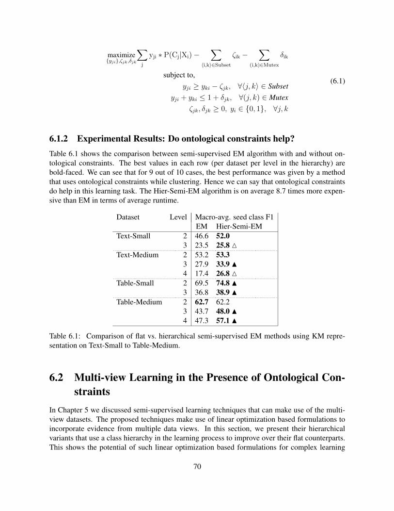
maximizeyji,ζjk,δjk

∑j

yji ∗ P(Cj|Xi)−∑

〈i,k〉∈Subset

ζik −∑

(i,k)∈Mutex

δik

subject to,yji ≥ yki − ζjk, ∀〈j, k〉 ∈ Subset

yji + yki ≤ 1 + δjk, ∀(j, k) ∈ Mutexζjk, δjk ≥ 0, yi ∈ 0, 1, ∀j, k

(6.1)

6.1.2 Experimental Results: Do ontological constraints help?Table 6.1 shows the comparison between semi-supervised EM algorithm with and without on-tological constraints. The best values in each row (per dataset per level in the hierarchy) arebold-faced. We can see that for 9 out of 10 cases, the best performance was given by a methodthat uses ontological constraints while clustering. Hence we can say that ontological constraintsdo help in this learning task. The Hier-Semi-EM algorithm is on average 8.7 times more expen-sive than EM in terms of average runtime.

Dataset Level Macro-avg. seed class F1EM Hier-Semi-EM

Text-Small 2 46.6 52.03 23.5 25.8 M

Text-Medium 2 53.2 53.33 27.9 33.9 N4 17.4 26.8 M

Table-Small 2 69.5 74.8 N3 36.8 38.9 N

Table-Medium 2 62.7 62.23 43.7 48.0 N4 47.3 57.1 N

Table 6.1: Comparison of flat vs. hierarchical semi-supervised EM methods using KM repre-sentation on Text-Small to Table-Medium.

6.2 Multi-view Learning in the Presence of Ontological Con-straints

In Chapter 5 we discussed semi-supervised learning techniques that can make use of the multi-view datasets. The proposed techniques make use of linear optimization based formulations toincorporate evidence from multiple data views. In this section, we present their hierarchicalvariants that use a class hierarchy in the learning process to improve over their flat counterparts.This shows the potential of such linear optimization based formulations for complex learning

70

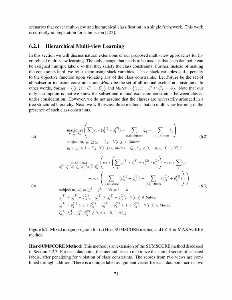
scenarios that cover multi-view and hierarchical classification in a single framework. This workis currently in preparation for submission [123].

6.2.1 Hierarchical Multi-view LearningIn this section we will discuss natural extensions of our proposed multi-view approaches for hi-erarchical multi-view learning. The only change that needs to be made is that each datapoint canbe assigned multiple labels, so that they satisfy the class constraints. Further, instead of makingthe constraints hard, we relax them using slack variables. These slack variables add a penaltyto the objective function upon violating any of the class constraints. Let Subset be the set ofall subset or inclusion constraints, and Mutex be the set of all mutual exclusion constraints. Inother words, Subset = 〈i, j〉 : Ci ⊆ Cj and Mutex = (i, j) : Ci ∩ Cj = φ. Note that ouronly assumption is that we know the subset and mutual exclusion constraints between classesunder consideration. However, we do not assume that the classes are necessarily arranged in atree structured hierarchy. Next, we will discuss three methods that do multi-view learning in thepresence of such class constraints.

(a)

maximizeyi,ζij ,δij

∑i

yi ∗ (s(1)i + s

(2)i )−

∑〈i,j〉∈Subset

ζij −∑

(i,j)∈Mutex

δij

subject to, yj ≥ yi − ζij , ∀〈i, j〉 ∈ Subset

yi + yj ≤ 1 + δij , ∀(i, j) ∈ Mutex, ζij , δij ≥ 0, yi ∈ 0, 1 ∀i, j

(6.2)

(b)

maximizey(1)i ,y

(2)i ,di,ζ

(1)ij ,δ

(1)ij ,ζ

(2)ij ,δ

(2)ij

(α1 ∗

(∑i

y(1)i ∗ s

(1)i + y

(2)i ∗ s

(2)i

)− α2 ∗

∑i

di

−α3 ∗

∑〈i,j〉∈Subset

(ζ(1)ij + ζ

(2)ij ) +

∑(i,j)∈Mutex

(δ(1)ij + δ

(2)ij )

)subject to, di = |y1

i − y2i |, ∀i = 1 . . . k

y(1)j ≥ y

(1)i − ζ

(1)ij , y

(2)j ≥ y

(2)i − ζ

(2)ij , ∀〈i, j〉 ∈ Subset

y(1)i + y

(1)j ≤ 1 + δ

(1)ij , y

(2)i + y

(2)j ≤ 1 + δ

(2)ij , ∀(i, j) ∈ Mutex

ζ(1)ij , δ

(1)ij , ζ

(2)ij , δ

(2)ij ≥ 0, yi ∈ 0, 1 ∀i, j

(6.3)

Figure 6.2: Mixed integer program for (a) Hier-SUMSCORE method and (b) Hier-MAXAGREEmethod.

Hier-SUMSCORE Method: This method is an extension of the SUMSCORE method discussedin Section 5.2.3. For each datapoint, this method tries to maximize the sum of scores of selectedlabels, after penalizing for violation of class constraints. The scores from two views are com-bined through addition. There is a unique label assignment vector for each datapoint across two

71

views computed by solving the mixed integer program given Equation 6.2 (Figure 6.2 (a)).

Hier-PRODSCORE Method: This method is an extension of the PRODSCORE method. Themixed integer program for this method is very similar to that of the Hier-SUMSCORE methodexcept that in the objective function, scores from two views are combined using product insteadof addition of scores. There is a unique label assignment vector for each datapoint across twoviews.

Hier-MAXAGREE Method: This is an immediate extension of the MAXAGREE method de-scribed in Section 5.2.3, to incorporate class hierarchy. Different views can assign a datapoint todifferent sets of clusters. There is a penalty on cluster assignments being different across views,and any violation of the class constraints. Equation 6.3 (Figure 6.2 (b)) shows the mixed integerlinear program to be solved for each datapoint. For each datapoint s(1)

i , s(2)i represent scores of

x belonging to cluster i; and y(1)i , y(2)

i represent cluster assignment of x in view 1 and view 2respectively. di is the penalty on y(1)

i and y(2)i being different. ζ(1)

ij and ζ(2)ij are the penalty terms

for Subset constraints. Similarly, δ(1)ij and δ(2)

ij are the penalty terms for Mutex constraints. α1, α2

and α3 are constants that define relative importance of terms in the objective function.Integer linear programming is used by several existing approaches to do constrained infer-

ence. [95] used mixed integer linear programming techniques to encode ontological constraints–they assign multiple plausible KB categories to ‘emerging’ entities, which are not yet repre-sented in the KB, and consider mutual exclusion constraints as a post-processing step, so as tooutput a consistent set of category assignments. On the other hand, our method jointly modelsmulti-view, subset and mutual exclusion constraints, within an iterative semi-supervised EM al-gorithm. Note that the hierarchical methods discussed here can work with any class ontologyand are not limited to tree structured ontologies.

6.2.2 Experimental Results

Note that out of the eight multi-view datasets we experimented with in Section 5.3 only NELL mvdataset is hierarchical. To test hierarchical multi-view methods, we performed experiments onthe NELL mv dataset with the training percentage varying from 5% to 30%. We generated 10random train/test partitions for each training percentage value. Both flat and hierarchical meth-ods got exactly the same train and test instances as input. Hierarchical methods had access to theentire hierarchy of labels and classified each datapoint w.r.t all classes in the hierarchy follow-ing the class constraints. Flat methods on the other hand learnt models only for the leaf classesof the hierarchy. We compared average F1 scores of all methods on the leaf classes. Further,we also compare these methods in terms of their average rank according to macro averaged F1scores. According to this metric, the Hier-MAXAGREE method is the best followed by Hier-SUMSCORE, and Hier-PRODSCORE.

Table 6.2 shows the macro-averaged F1 results for all methods varying the training percent-age. We can see that all the proposed hierarchical methods Hier-SUMSCORE, Hier-PRODSCOREand Hier-MAXAGREE improve over their flat counterparts in terms of macro-averaged F1 scoresfor all values of the training percentage. Columns marked as ∆ shows the percentage relative

72

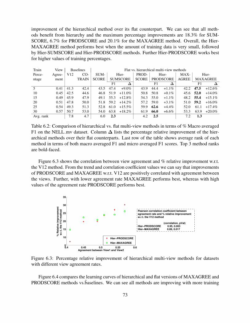
improvement of the hierarchical method over its flat counterpart. We can see that all meth-ods benefit from hierarchy and the maximum percentage improvements are 18.3% for SUM-SCORE, 6.7% for PRODSCORE and 20.1% for the MAXAGREE method. Overall, the Hier-MAXAGREE method performs best when the amount of training data is very small, followedby Hier-SUMSCORE and Hier-PRODSCORE methods. Further Hier-PRODSCORE works bestfor higher values of training percentages.

Train View Baselines Flat vs. hierarchical multi-view methodsPerce- Agree- V12 CO- SUM- Hier- PROD- Hier- MAX- Hier-ntage ment TRAIN SCORE SUMSCORE SCORE PRODSCORE AGREE MAXAGREE

F1 ∆ F1 ∆ F1 ∆5 0.41 41.3 42.4 43.5 47.4 +9.0% 43.9 44.4 +1.1% 42.2 47.5 +12.6%10 0.45 42.5 44.6 46.8 51.9 +11.0% 50.8 50.8 +0.1% 45.6 52.0 +14.0%15 0.49 45.9 47.9 49.1 55.3 +12.8% 54.3 55.0 +1.1% 48.2 55.4 +15.1%20 0.51 47.8 50.0 51.8 59.2 +14.2% 57.2 59.0 +3.1% 51.0 59.2 +16.0%25 0.54 49.3 51.3 52.8 61.0 +15.5% 59.9 62.6 +4.4% 52.0 61.1 +17.4%30 0.57 50.7 53.0 54.0 63.8 +18.2% 61.9 66.0 +6.6% 53.3 63.9 +20.0%Avg. rank 7.8 4.7 6.0 2.3 4.2 2.5 7.2 1.3

Table 6.2: Comparison of hierarchical vs. flat multi-view methods in terms of % Macro averagedF1 on the NELL mv dataset. Column ∆ lists the percentage relative improvement of the hier-archical methods over their flat counterparts. Last row of the table shows average rank of eachmethod in terms of both macro averaged F1 and micro averaged F1 scores. Top 3 method ranksare bold-faced.

Figure 6.3 shows the correlation between view agreement and % relative improvement w.r.t.the V12 method. From the trend and correlation coefficient values we can say that improvementsof PRODSCORE and MAXAGREE w.r.t. V12 are positively correlated with agreement betweenthe views. Further, with lower agreement rate MAXAGREE performs best, whereas with highvalues of the agreement rate PRODSCORE performs best.

0.4 0.45 0.5 0.55 0.65

10

15

20

25

30

35

Agreement between View1 and View2

% R

ela

tive im

pro

vem

en

t w

.r.t

. th

e V

12 m

eth

od

Hier−PRODSCORE

Hier−MAXAGREE

Pearson correlation coefficient between agreement rate and % relative improvementw.r.t. the V12 method

(correlation, pVal)Hier−PRODSCORE 0.95, 0.003Hier−MAXAGREE 0.89, 0.017

Figure 6.3: Percentage relative improvement of hierarchical multi-view methods for datasetswith different view agreement rates.

Figure 6.4 compares the learning curves of hierarchical and flat versions of MAXAGREE andPRODSCORE methods vs.baselines. We can see all methods are improving with more training

73

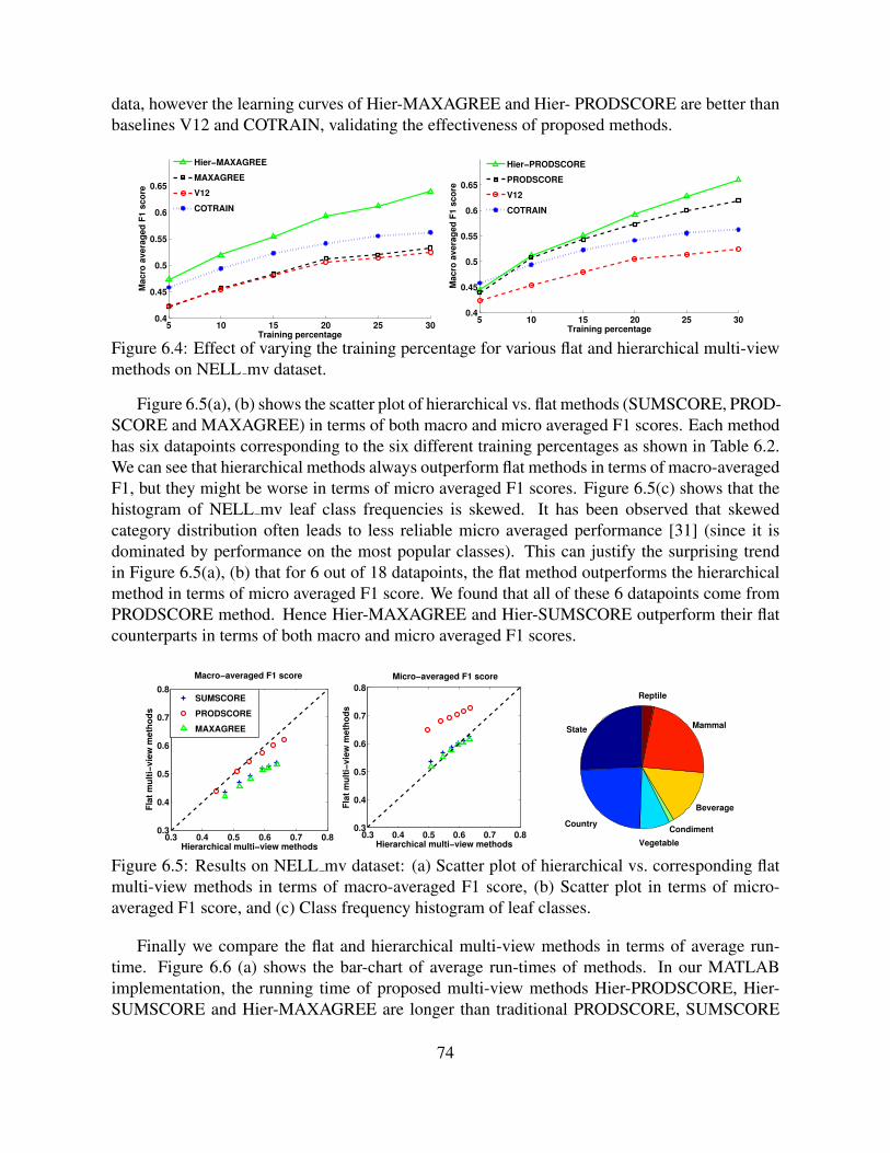
data, however the learning curves of Hier-MAXAGREE and Hier- PRODSCORE are better thanbaselines V12 and COTRAIN, validating the effectiveness of proposed methods.

5 10 15 20 25 300.4

0.45

0.5

0.55

0.6

0.65

Training percentage

Ma

cro

av

era

ge

d F

1 s

co

re

Hier−MAXAGREE

MAXAGREE

V12

COTRAIN

5 10 15 20 25 300.4

0.45

0.5

0.55

0.6

0.65

Training percentage

Ma

cro

av

era

ge

d F

1 s

co

re

Hier−PRODSCORE

PRODSCORE

V12

COTRAIN

Figure 6.4: Effect of varying the training percentage for various flat and hierarchical multi-viewmethods on NELL mv dataset.

Figure 6.5(a), (b) shows the scatter plot of hierarchical vs. flat methods (SUMSCORE, PROD-SCORE and MAXAGREE) in terms of both macro and micro averaged F1 scores. Each methodhas six datapoints corresponding to the six different training percentages as shown in Table 6.2.We can see that hierarchical methods always outperform flat methods in terms of macro-averagedF1, but they might be worse in terms of micro averaged F1 scores. Figure 6.5(c) shows that thehistogram of NELL mv leaf class frequencies is skewed. It has been observed that skewedcategory distribution often leads to less reliable micro averaged performance [31] (since it isdominated by performance on the most popular classes). This can justify the surprising trendin Figure 6.5(a), (b) that for 6 out of 18 datapoints, the flat method outperforms the hierarchicalmethod in terms of micro averaged F1 score. We found that all of these 6 datapoints come fromPRODSCORE method. Hence Hier-MAXAGREE and Hier-SUMSCORE outperform their flatcounterparts in terms of both macro and micro averaged F1 scores.

0.3 0.4 0.5 0.6 0.7 0.80.3

0.4

0.5

0.6

0.7

0.8

Hierarchical multi−view methods

Fla

t m

ult

i−v

iew

me

tho

ds

0.3 0.4 0.5 0.6 0.7 0.80.3

0.4

0.5

0.6

0.7

0.8

Hierarchical multi−view methods

Fla

t m

ult

i−v

iew

me

tho

ds

SUMSCORE

PRODSCORE

MAXAGREE

Macro−averaged F1 score Micro−averaged F1 score

State

Country

Vegetable

Condiment

Beverage

Mammal

Reptile

Figure 6.5: Results on NELL mv dataset: (a) Scatter plot of hierarchical vs. corresponding flatmulti-view methods in terms of macro-averaged F1 score, (b) Scatter plot in terms of micro-averaged F1 score, and (c) Class frequency histogram of leaf classes.

Finally we compare the flat and hierarchical multi-view methods in terms of average run-time. Figure 6.6 (a) shows the bar-chart of average run-times of methods. In our MATLABimplementation, the running time of proposed multi-view methods Hier-PRODSCORE, Hier-SUMSCORE and Hier-MAXAGREE are longer than traditional PRODSCORE, SUMSCORE

74

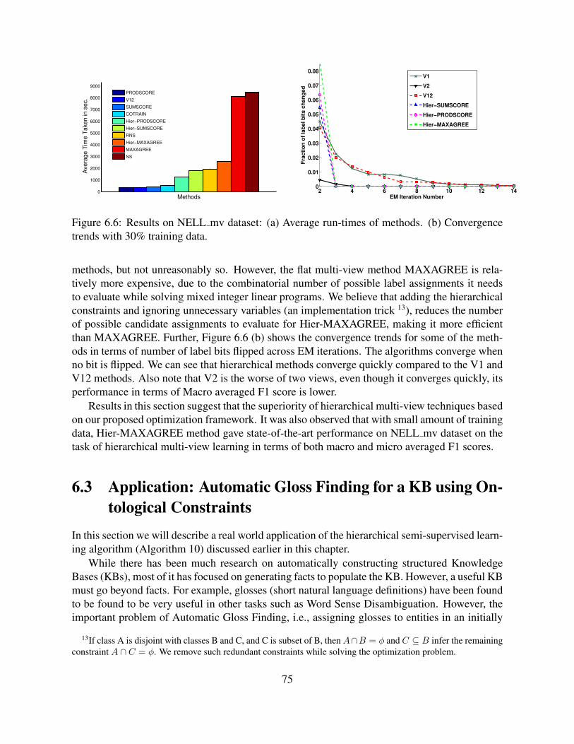
0

1000

2000

3000

4000

5000

6000

7000

8000

9000

Methods

Ave

rag

e T

ime

Ta

ke

n in

se

c.

PRODSCORE

V12

SUMSCORE

COTRAIN

Hier−PRODSCORE

Hier−SUMSCORE

RNS

Hier−MAXAGREE

MAXAGREE

NS

2 4 6 8 10 12 140

0.01

0.02

0.03

0.04

0.05

0.06

0.07

0.08

EM Iteration Number

Fra

cti

on

of

lab

el

bit

s c

ha

ng

ed

V1

V2

V12

Hier−SUMSCORE

Hier−PRODSCORE

Hier−MAXAGREE

Figure 6.6: Results on NELL mv dataset: (a) Average run-times of methods. (b) Convergencetrends with 30% training data.

methods, but not unreasonably so. However, the flat multi-view method MAXAGREE is rela-tively more expensive, due to the combinatorial number of possible label assignments it needsto evaluate while solving mixed integer linear programs. We believe that adding the hierarchicalconstraints and ignoring unnecessary variables (an implementation trick 13), reduces the numberof possible candidate assignments to evaluate for Hier-MAXAGREE, making it more efficientthan MAXAGREE. Further, Figure 6.6 (b) shows the convergence trends for some of the meth-ods in terms of number of label bits flipped across EM iterations. The algorithms converge whenno bit is flipped. We can see that hierarchical methods converge quickly compared to the V1 andV12 methods. Also note that V2 is the worse of two views, even though it converges quickly, itsperformance in terms of Macro averaged F1 score is lower.

Results in this section suggest that the superiority of hierarchical multi-view techniques basedon our proposed optimization framework. It was also observed that with small amount of trainingdata, Hier-MAXAGREE method gave state-of-the-art performance on NELL mv dataset on thetask of hierarchical multi-view learning in terms of both macro and micro averaged F1 scores.

6.3 Application: Automatic Gloss Finding for a KB using On-tological Constraints

In this section we will describe a real world application of the hierarchical semi-supervised learn-ing algorithm (Algorithm 10) discussed earlier in this chapter.

While there has been much research on automatically constructing structured KnowledgeBases (KBs), most of it has focused on generating facts to populate the KB. However, a useful KBmust go beyond facts. For example, glosses (short natural language definitions) have been foundto be found to be very useful in other tasks such as Word Sense Disambiguation. However, theimportant problem of Automatic Gloss Finding, i.e., assigning glosses to entities in an initially

13If class A is disjoint with classes B and C, and C is subset of B, then A∩B = φ and C ⊆ B infer the remainingconstraint A ∩ C = φ. We remove such redundant constraints while solving the optimization problem.

75

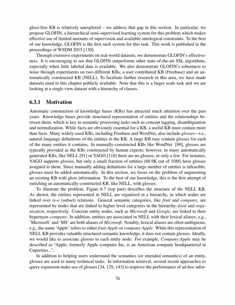
gloss-free KB is relatively unexplored – we address that gap in this section. In particular, wepropose GLOFIN, a hierarchical semi-supervised learning system for this problem which makeseffective use of limited amounts of supervision and available ontological constraints. To the bestof our knowledge, GLOFIN is the first such system for this task. This work is published in theproceedings of WSDM 2015 [130].

Through extensive experiments on real-world datasets, we demonstrate GLOFIN’s effective-ness. It is encouraging to see that GLOFIN outperforms other state-of-the-art SSL algorithms,especially when little labeled data is available. We also demonstrate GLOFIN’s robustness tonoise through experiments on two different KBs, a user contributed KB (Freebase) and an au-tomatically constructed KB (NELL). To facilitate further research in this area, we have madedatasets used in this chapter publicly available. Note that this is a larger scale task and we arelooking at a single view dataset with a hierarchy of classes.

6.3.1 MotivationAutomatic construction of knowledge bases (KBs) has attracted much attention over the pastyears. Knowledge bases provide structured representation of entities and the relationships be-tween them, which is key in semantic processing tasks such as concept tagging, disambiguationand normalization. While facts are obviously essential for a KB, a useful KB must contain morethan facts. Many widely-used KBs, including Freebase and WordNet, also include glosses—i.e.,natural language definitions of the entities in the KB. A large KB may contain glosses for eachof the many entities it contains. In manually-constructed KBs like WordNet [90], glosses aretypically provided as the KBs constructed by human experts; however, in many automaticallygenerated KBs, like NELL [91] or YAGO [118] there are no glosses, or only a few. For instance,YAGO supports glosses, but only a small fraction of entities (68.9K out of 10M) have glossesassigned to them. Since manually adding definitions for a large number of entities is infeasible,glosses must be added automatically. In this section, we focus on the problem of augmentingan existing KB with gloss information. To the best of our knowledge, this is the first attempt ofenriching an automatically-constructed KB, like NELL, with glosses.

To illustrate the problem, Figure 6.7 (top part) describes the structure of the NELL KB.As shown, the entities represented in NELL are organized in a hierarchy, in which nodes arelinked over is-a (subset) relations. General semantic categories, like fruit and company, arerepresented by nodes that are linked to higher level categories in the hierarchy–food and orga-nization, respectively. Concrete entity nodes, such as Microsoft and Google, are linked to theirhypernym–company. In addition, entities are associated in NELL with their lexical aliases; e.g.,‘Microsoft’ and ‘MS’ are both aliases of Microsoft. Notably, lexical aliases are often ambiguous,e.g., the name ‘Apple’ refers to either fruit:Apple or company:Apple. While this representation ofNELL KB provides valuable structured semantic knowledge, it does not contain glosses. Ideally,we would like to associate glosses to each entity node. For example, Company:Apple may bedescribed as “Apple, formerly Apple computer Inc, is an American company headquartered inCupertino...”.

In addition to helping users understand the semantics (or intended semantics) of an entity,glosses are used in many technical tasks. In information retrieval, several recent approaches toquery expansion make use of glosses [34, 129, 143] to improve the performance of ad-hoc infor-

76

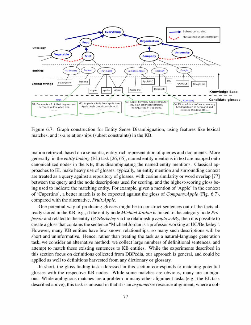
Figure 6.7: Graph construction for Entity Sense Disambiguation, using features like lexicalmatches, and is-a relationships (subset constraints) in the KB.

mation retrieval, based on a semantic, entity-rich representation of queries and documents. Moregenerally, in the entity linking (EL) task [26, 65], named entity mentions in text are mapped ontocanonicalized nodes in the KB, thus disambiguating the named entity mentions. Classical ap-proaches to EL make heavy use of glosses: typically, an entity mention and surrounding contextare treated as a query against a repository of glosses, with cosine similarity or word overlap [77]between the query and the node descriptions used for scoring, and the highest-scoring gloss be-ing used to indicate the matching entity. For example, given a mention of ‘Apple’ in the contextof ‘Cupertino’, a better match is to be expected against the gloss of Company:Apple (Fig. 6.7),compared with the alternative, Fruit:Apple.

One potential way of producing glosses might be to construct sentences out of the facts al-ready stored in the KB: e.g., if the entity node Michael Jordan is linked to the category node Pro-fessor and related to the entity UC/Berkeley via the relationship employedBy, then it is possible tocreate a gloss that contains the sentence “Michael Jordan is a professor working at UC/Berkeley”.However, many KB entities have few known relationships, so many such descriptions will beshort and uninformative. Hence, rather than treating the task as a natural-language generationtask, we consider an alternative method: we collect large numbers of definitional sentences, andattempt to match these existing sentences to KB entities. While the experiments described inthis section focus on definitions collected from DBPedia, our approach is general, and could beapplied as well to definitions harvested from any dictionary or glossary.

In short, the gloss finding task addressed in this section corresponds to matching potentialglosses with the respective KB nodes. While some matches are obvious, many are ambigu-ous. While ambiguous matches are a problem in many other alignment tasks (e.g., the EL taskdescribed above), this task is unusual in that it is an asymmetric resource alignment, where a col-

77

lection of lexical glosses, which contain no structure information, is aligned against a structuralKB, which contains no textual descriptions.

We define and address this task using semi-supervised learning (SSL) techniques. We relyon several simple intuitions to solve the above mentioned problem. First, it has already beenobserved [95, 118] that entity ambiguity is often resolved given its semantic category. Hence,rather than target a named entity linking problem, we solve an entity categorization problem.Next, we use the unambiguous glosses as labeled data for this entity categorization task. How-ever, such labeled data is limited and noisy. We therefore propose Gloss Finder (GLOFIN)method for this task, which internally uses the semi-supervised Expectation Maximization (EM)method described in Algorithm 10.

6.3.2 Automatic Gloss Finding (GLOFIN)

In this section, we describe GLOFIN, our approach to the Gloss Finding problem. We firstdescribe an entity-gloss candidate generation stage whose output is used by all the methodsconsidered in the section.

Candidate Entity-Gloss Generation

In this step, for each gloss in the candidate pool of glosses given as input, we first identify thenoun phrase that is being defined by the gloss. We refer to this noun phrase as head-NP in thissection. For DBPedia abstracts this step is trivial in the sense that DBPedia dataset gives us thehead-NP for each short abstract. However, we can easily apply existing syntactic taggers, e.g.,the Stanford tagger [83], and detect the head-NP in the definitional sentence(s). After this, thehead NP of each gloss is lexically matched against the entities in the KB. Even though simplestring matchings are used for the experiments here, more sophisticated string matchers may alsobe used.

At the end of this stage, we end up with a set of candidate entity-gloss matchings. Please notethat this relationship may be many-many and thereby ambiguous as one entity may be connectedto multiple glosses, and a single gloss may be assigned multiple entities. Such ambiguity areresolved using the techniques described below.

Proposed Approach: Gloss Finder (GLOFIN)

Our Gloss Finder (GLOFIN) method uses the hierarchical semi-supervised Expectation Maxi-mization (EM) algorithm (refer to Algorithm 10) to classify glosses into KB categories whilesatisfying ontological constraints. GLOFIN uses automatically acquired labeled data (unam-biguous candidate glosses) and large amount of unlabeled data (rest of the candidate glosses)in an iterative EM framework to learn a model for this task. The hierarchical semi-supervisedExpectation Maximization (EM) algorithm uses the MIP formulation (Equation 6.1) to get thebest label vector for each datapoint.

78

Scaling GLOFIN

Note that, the MIP formulation presented in Equation 6.1 adds a constraint per subset and mutualexclusion constraints in the KB ontology. Further, in the E step of every iteration, we solve a MIPper gloss. These two result in longer runtimes for this method. We make our method scalableand efficient in following ways:• We discard the redundant mutex constraints, the ones that can be inferred using remaining

subset and mutex constraints.• We reduce the number of classes considered per gloss, by keeping only top-Q classes relevant

to the gloss, as detailed below.• Since MIP for each gloss is independent, we parallelize the E step of every iteration, and con-

solidate results in the M-step.

Reducing the MIP size per gloss: We keep only a small number of categories in the optimiza-tion problem that is being solved for each gloss. We tried the following three ways of keepingonly some of the candidate classes:• Diameter of the class graph: The class graph is an undirected graph of ontology classes, where

nodes are classes and edges represent either subset or mutual exclusion constraints. In thisapproximation, we rank all classes by the scores P (Cj|Xi) for a datapoint Xi, and choose thetop Q classes, where Q is the diameter of the category graph. Since the class assignments arehierarchical, we also include all ancestors of these top-Q classes in the optimization.• Square-root of number of classes: Here, we select Q =

√K, where K is the total number of

classes in the ontology. Similar to diameter based method, we include all ancestors of thesetop-Q classes in the optimization.• Thresholding: If the score P (Cj|Xi) is greater than a predefined threshold then we consider

the category. Note that the threshold is set for the entire dataset, so for each datapoint, it mightresult in a different number of categories and constraints.

6.3.3 Datasets and Experimental MethodologyIn our experiments, we enrich two existing knowledge bases with available glosses, namelyNELL and Freebase. NELL is a machine generated knowledge base that does not have existingglosses, whereas most Freebase entities have descriptions/glosses we can compare against. Ourresource of glosses is DBPedia, a database of factual descriptions extracted from Wikipediaeditions in 97 different languages. DBPedia contains a large set of Wikipedia titles and shortabstracts.

A DBPedia short abstract of an entity is essentially the first paragraph (up to 500 characters)on the Wikipedia page of that entity. Some sample entity titles and their corresponding DBPediaabstracts are given in Table 6.3.

We now describe two experimental datasets that were labeled for evaluation purposes. Wehave made both these gloss finding datasets available14 for the research community to help the

14The dataset can be downloaded from http://rtw.ml.cmu.edu/wk/WebSets/glossFinding_wsdm_2015_online/index.html

79

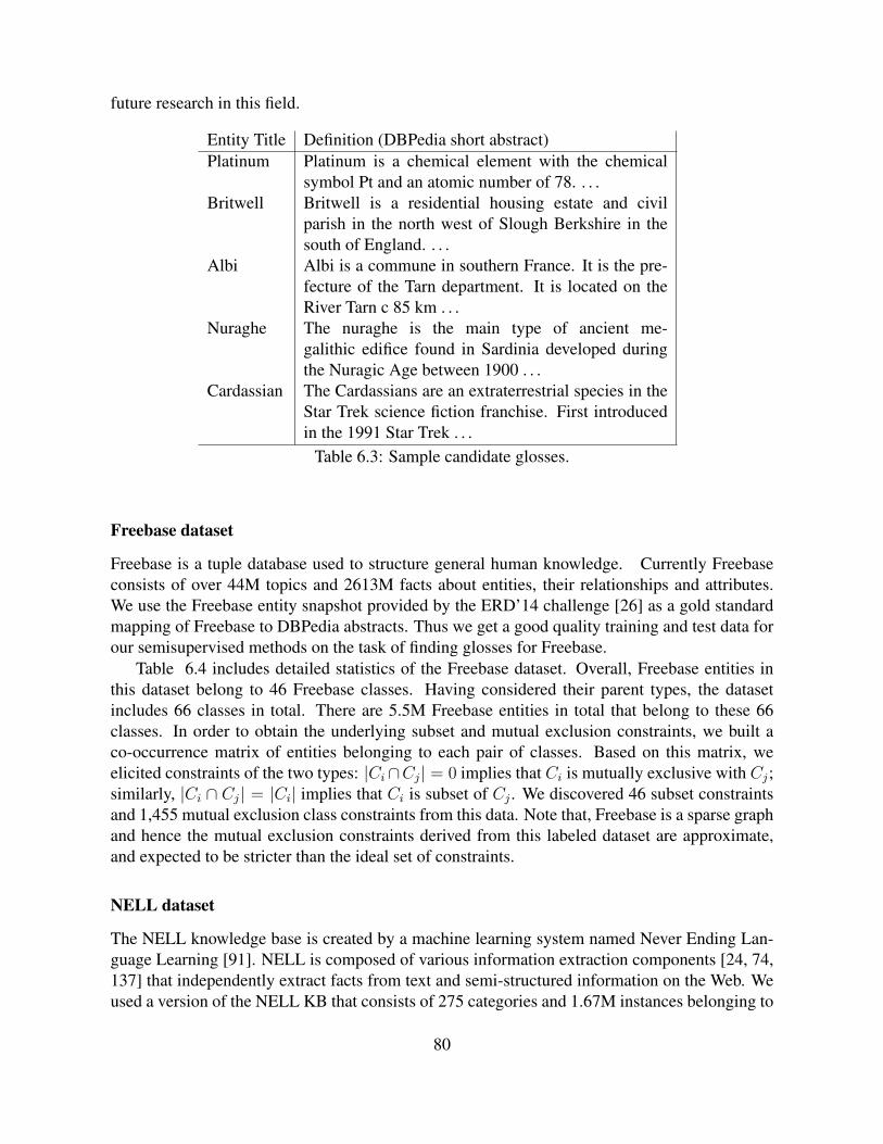
future research in this field.

Entity Title Definition (DBPedia short abstract)Platinum Platinum is a chemical element with the chemical

symbol Pt and an atomic number of 78. . . .Britwell Britwell is a residential housing estate and civil

parish in the north west of Slough Berkshire in thesouth of England. . . .

Albi Albi is a commune in southern France. It is the pre-fecture of the Tarn department. It is located on theRiver Tarn c 85 km . . .

Nuraghe The nuraghe is the main type of ancient me-galithic edifice found in Sardinia developed duringthe Nuragic Age between 1900 . . .

Cardassian The Cardassians are an extraterrestrial species in theStar Trek science fiction franchise. First introducedin the 1991 Star Trek . . .

Table 6.3: Sample candidate glosses.

Freebase dataset

Freebase is a tuple database used to structure general human knowledge. Currently Freebaseconsists of over 44M topics and 2613M facts about entities, their relationships and attributes.We use the Freebase entity snapshot provided by the ERD’14 challenge [26] as a gold standardmapping of Freebase to DBPedia abstracts. Thus we get a good quality training and test data forour semisupervised methods on the task of finding glosses for Freebase.

Table 6.4 includes detailed statistics of the Freebase dataset. Overall, Freebase entities inthis dataset belong to 46 Freebase classes. Having considered their parent types, the datasetincludes 66 classes in total. There are 5.5M Freebase entities in total that belong to these 66classes. In order to obtain the underlying subset and mutual exclusion constraints, we built aco-occurrence matrix of entities belonging to each pair of classes. Based on this matrix, weelicited constraints of the two types: |Ci∩Cj| = 0 implies that Ci is mutually exclusive with Cj;similarly, |Ci ∩ Cj| = |Ci| implies that Ci is subset of Cj . We discovered 46 subset constraintsand 1,455 mutual exclusion class constraints from this data. Note that, Freebase is a sparse graphand hence the mutual exclusion constraints derived from this labeled dataset are approximate,and expected to be stricter than the ideal set of constraints.

NELL dataset

The NELL knowledge base is created by a machine learning system named Never Ending Lan-guage Learning [91]. NELL is composed of various information extraction components [24, 74,137] that independently extract facts from text and semi-structured information on the Web. Weused a version of the NELL KB that consists of 275 categories and 1.67M instances belonging to

80

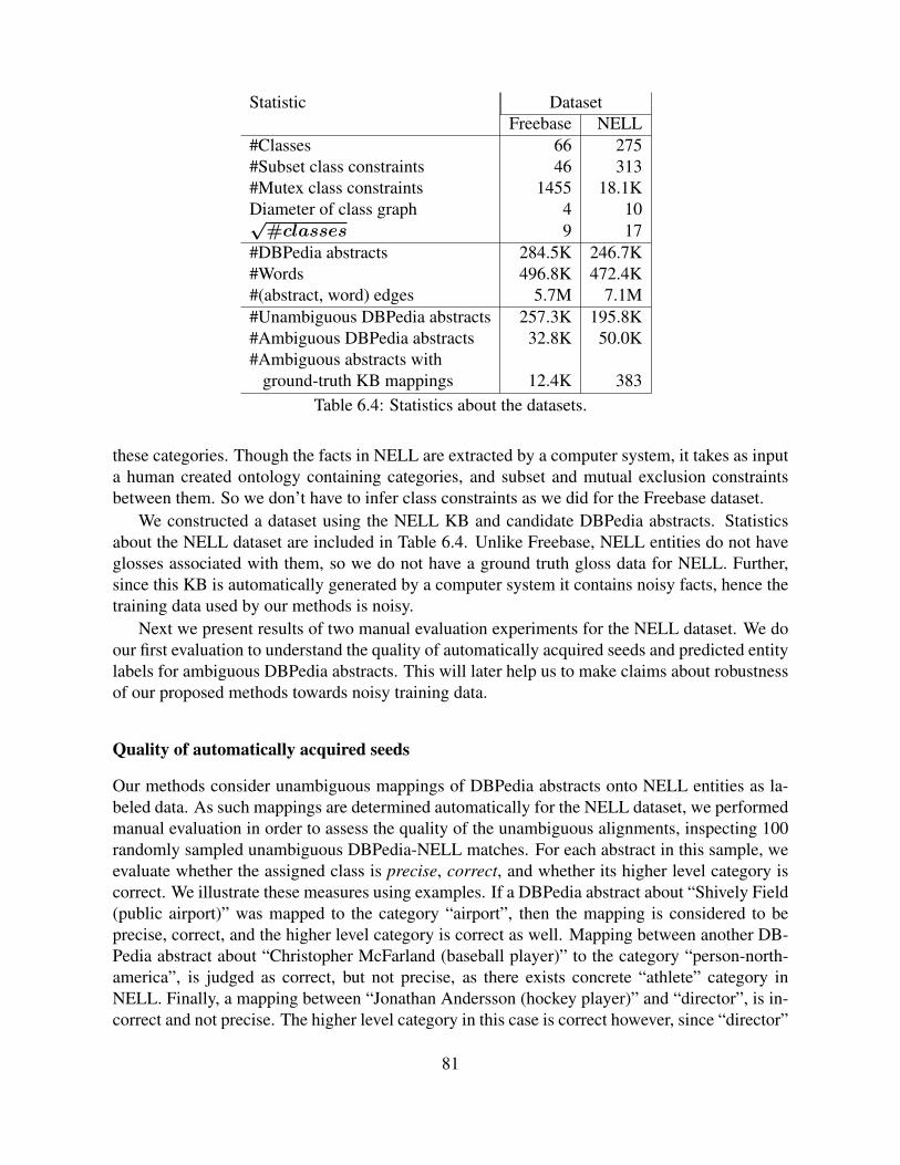
Statistic DatasetFreebase NELL

#Classes 66 275#Subset class constraints 46 313#Mutex class constraints 1455 18.1KDiameter of class graph 4 10√

#classes 9 17#DBPedia abstracts 284.5K 246.7K#Words 496.8K 472.4K#(abstract, word) edges 5.7M 7.1M#Unambiguous DBPedia abstracts 257.3K 195.8K#Ambiguous DBPedia abstracts 32.8K 50.0K#Ambiguous abstracts with

ground-truth KB mappings 12.4K 383Table 6.4: Statistics about the datasets.

these categories. Though the facts in NELL are extracted by a computer system, it takes as inputa human created ontology containing categories, and subset and mutual exclusion constraintsbetween them. So we don’t have to infer class constraints as we did for the Freebase dataset.

We constructed a dataset using the NELL KB and candidate DBPedia abstracts. Statisticsabout the NELL dataset are included in Table 6.4. Unlike Freebase, NELL entities do not haveglosses associated with them, so we do not have a ground truth gloss data for NELL. Further,since this KB is automatically generated by a computer system it contains noisy facts, hence thetraining data used by our methods is noisy.

Next we present results of two manual evaluation experiments for the NELL dataset. We doour first evaluation to understand the quality of automatically acquired seeds and predicted entitylabels for ambiguous DBPedia abstracts. This will later help us to make claims about robustnessof our proposed methods towards noisy training data.

Quality of automatically acquired seeds

Our methods consider unambiguous mappings of DBPedia abstracts onto NELL entities as la-beled data. As such mappings are determined automatically for the NELL dataset, we performedmanual evaluation in order to assess the quality of the unambiguous alignments, inspecting 100randomly sampled unambiguous DBPedia-NELL matches. For each abstract in this sample, weevaluate whether the assigned class is precise, correct, and whether its higher level category iscorrect. We illustrate these measures using examples. If a DBPedia abstract about “Shively Field(public airport)” was mapped to the category “airport”, then the mapping is considered to beprecise, correct, and the higher level category is correct as well. Mapping between another DB-Pedia abstract about “Christopher McFarland (baseball player)” to the category “person-north-america”, is judged as correct, but not precise, as there exists concrete “athlete” category inNELL. Finally, a mapping between “Jonathan Andersson (hockey player)” and “director”, is in-correct and not precise. The higher level category in this case is correct however, since “director”

81

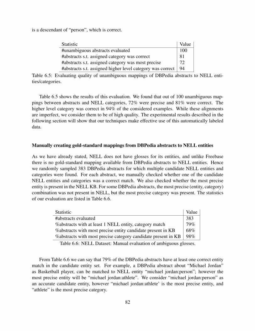
is a descendant of “person”, which is correct.

Statistic Value#unambiguous abstracts evaluated 100#abstracts s.t. assigned category was correct 81#abstracts s.t. assigned category was most precise 72#abstracts s.t. assigned higher level category was correct 94

Table 6.5: Evaluating quality of unambiguous mappings of DBPedia abstracts to NELL enti-ties/categories.

Table 6.5 shows the results of this evaluation. We found that out of 100 unambiguous map-pings between abstracts and NELL categories, 72% were precise and 81% were correct. Thehigher level category was correct in 94% of the considered examples. While these alignmentsare imperfect, we consider them to be of high quality. The experimental results described in thefollowing section will show that our techniques make effective use of this automatically labeleddata.

Manually creating gold-standard mappings from DBPedia abstracts to NELL entities

As we have already stated, NELL does not have glosses for its entities, and unlike Freebasethere is no gold-standard mapping available from DBPedia abstracts to NELL entities. Hencewe randomly sampled 383 DBPedia abstracts for which multiple candidate NELL entities andcategories were found. For each abstract, we manually checked whether one of the candidateNELL entities and categories was a correct match. We also checked whether the most preciseentity is present in the NELL KB. For some DBPedia abstracts, the most precise (entity, category)combination was not present in NELL, but the most precise category was present. The statisticsof our evaluation are listed in Table 6.6.

Statistic Value#abstracts evaluated 383%abstracts with at least 1 NELL entity, category match 79%%abstracts with most precise entity candidate present in KB 68%%abstracts with most precise category candidate present in KB 98%

Table 6.6: NELL Dataset: Manual evaluation of ambiguous glosses.

From Table 6.6 we can say that 79% of the DBPedia abstracts have at least one correct entitymatch in the candidate entity set. For example, a DBPedia abstract about “Michael Jordan”as Basketball player, can be matched to NELL entity “michael jordan:person”; however themost precise entity will be “michael jordan:athlete”. We consider “michael jordan:person” asan accurate candidate entity, however “michael jordan:athlete’ is the most precise entity, and“athlete” is the most precise category.

82

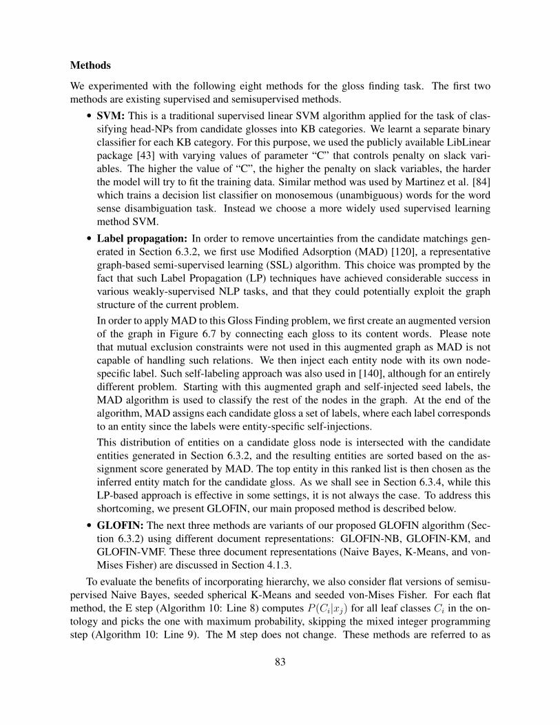
Methods

We experimented with the following eight methods for the gloss finding task. The first twomethods are existing supervised and semisupervised methods.• SVM: This is a traditional supervised linear SVM algorithm applied for the task of clas-

sifying head-NPs from candidate glosses into KB categories. We learnt a separate binaryclassifier for each KB category. For this purpose, we used the publicly available LibLinearpackage [43] with varying values of parameter “C” that controls penalty on slack vari-ables. The higher the value of “C”, the higher the penalty on slack variables, the harderthe model will try to fit the training data. Similar method was used by Martinez et al. [84]which trains a decision list classifier on monosemous (unambiguous) words for the wordsense disambiguation task. Instead we choose a more widely used supervised learningmethod SVM.

• Label propagation: In order to remove uncertainties from the candidate matchings gen-erated in Section 6.3.2, we first use Modified Adsorption (MAD) [120], a representativegraph-based semi-supervised learning (SSL) algorithm. This choice was prompted by thefact that such Label Propagation (LP) techniques have achieved considerable success invarious weakly-supervised NLP tasks, and that they could potentially exploit the graphstructure of the current problem.In order to apply MAD to this Gloss Finding problem, we first create an augmented versionof the graph in Figure 6.7 by connecting each gloss to its content words. Please notethat mutual exclusion constraints were not used in this augmented graph as MAD is notcapable of handling such relations. We then inject each entity node with its own node-specific label. Such self-labeling approach was also used in [140], although for an entirelydifferent problem. Starting with this augmented graph and self-injected seed labels, theMAD algorithm is used to classify the rest of the nodes in the graph. At the end of thealgorithm, MAD assigns each candidate gloss a set of labels, where each label correspondsto an entity since the labels were entity-specific self-injections.This distribution of entities on a candidate gloss node is intersected with the candidateentities generated in Section 6.3.2, and the resulting entities are sorted based on the as-signment score generated by MAD. The top entity in this ranked list is then chosen as theinferred entity match for the candidate gloss. As we shall see in Section 6.3.4, while thisLP-based approach is effective in some settings, it is not always the case. To address thisshortcoming, we present GLOFIN, our main proposed method is described below.

• GLOFIN: The next three methods are variants of our proposed GLOFIN algorithm (Sec-tion 6.3.2) using different document representations: GLOFIN-NB, GLOFIN-KM, andGLOFIN-VMF. These three document representations (Naive Bayes, K-Means, and von-Mises Fisher) are discussed in Section 4.1.3.

To evaluate the benefits of incorporating hierarchy, we also consider flat versions of semisu-pervised Naive Bayes, seeded spherical K-Means and seeded von-Mises Fisher. For each flatmethod, the E step (Algorithm 10: Line 8) computes P (Ci|xj) for all leaf classes Ci in the on-tology and picks the one with maximum probability, skipping the mixed integer programmingstep (Algorithm 10: Line 9). The M step does not change. These methods are referred to as

83

GLOFIN-flat-NB, GLOFIN-flat-KM and GLOFIN-flat-VMF.

Features

Each gloss can be represented by the term frequency (TF) of words that occurred in it. Wecan also collect the inverse document frequency (IDF) of each word in the vocabulary fromthe entire gloss corpus. This gives us a choice of using either TF (mere term frequencies) orTFIDF (multiplication of TF and IDF values) feature representations. We use the TFIDF valuesto threshold the words used for each gloss. For all the experiments presented here, we keep onlythose words per gloss that cross TFIDF threshold15 of 1E-3, thereby discarding stop-words andother unimportant words.

For each method, we performed experiments with both TF and TFIDF based feature rep-resentations (considering only those words that pass TFIDF threshold). In our experiments wefound that SVM and Label-propagation methods give better performance for the TFIDF basedfeature representation, whereas all semisupervised EM methods (GLOFIN variants) work bestwith a TF based feature representation. Henceforth, we present all results using these choices offeature representations.

6.3.4 Experimental Results

Gloss Finding Results

In this section we present experimental results on the gloss finding task. For the first set of resultswe use all unambiguous glosses (glosses with only one candidate entity mapping to the KB) astraining data. The next set of experiments make use of only 10% of unambiguous matches astraining data. We compare all eight methods that we presented in Section 6.3.2: SVM, labelpropagation, the hierarchical and flat variants of GLOFIN.

For the SVM method, we tried different values of ‘C’ for the LibLinear package. We observedthe change in performance varying the values of ‘C’ in the range [1E-24, 100] for both datasets.The change in performance for different values of C for both datasets, is plotted in Figure 6.8.We found that the best performance is achieved for ‘C’ in the range [1E-6, 0.01]. The resultspresented here are with C = 1E-6.

From the experiments presented here, we try to answer the following research questions:

• How does our proposed GLOFIN-NB method compare with SVM and label propagation onthe task of assigning glosses for NELL and Freebase datasets?• How do the Naive Bayes, K-Means and von Mises-Fisher variants of GLOFIN method com-

pare?• Does the use of ontological constraints always improve results for GLOFIN method?• What is the effect of the different strategies of limiting the set of considered classes per gloss

on scalability (and performance) of GLOFIN method?

15After this filtering step, each candidate gloss in the NELL dataset has on average 30 unique words.

84

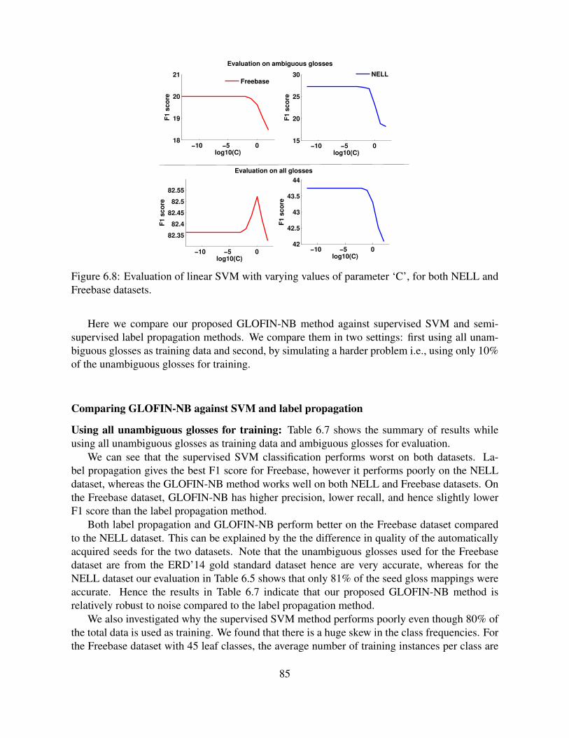
−10 −5 018

19

20

21

log10(C)

F1 s

co

re

−10 −5 015

20

25

30

log10(C)

F1 s

co

re

−10 −5 0

82.35

82.4

82.45

82.5

82.55

log10(C)

F1

sco

re

−10 −5 042

42.5

43

43.5

44

log10(C)

F1 s

co

re

FreebaseNELL

Evaluation on ambiguous glosses

Evaluation on all glosses

Figure 6.8: Evaluation of linear SVM with varying values of parameter ‘C’, for both NELL andFreebase datasets.

Here we compare our proposed GLOFIN-NB method against supervised SVM and semi-supervised label propagation methods. We compare them in two settings: first using all unam-biguous glosses as training data and second, by simulating a harder problem i.e., using only 10%of the unambiguous glosses for training.

Comparing GLOFIN-NB against SVM and label propagation

Using all unambiguous glosses for training: Table 6.7 shows the summary of results whileusing all unambiguous glosses as training data and ambiguous glosses for evaluation.

We can see that the supervised SVM classification performs worst on both datasets. La-bel propagation gives the best F1 score for Freebase, however it performs poorly on the NELLdataset, whereas the GLOFIN-NB method works well on both NELL and Freebase datasets. Onthe Freebase dataset, GLOFIN-NB has higher precision, lower recall, and hence slightly lowerF1 score than the label propagation method.

Both label propagation and GLOFIN-NB perform better on the Freebase dataset comparedto the NELL dataset. This can be explained by the the difference in quality of the automaticallyacquired seeds for the two datasets. Note that the unambiguous glosses used for the Freebasedataset are from the ERD’14 gold standard dataset hence are very accurate, whereas for theNELL dataset our evaluation in Table 6.5 shows that only 81% of the seed gloss mappings wereaccurate. Hence the results in Table 6.7 indicate that our proposed GLOFIN-NB method isrelatively robust to noise compared to the label propagation method.

We also investigated why the supervised SVM method performs poorly even though 80% ofthe total data is used as training. We found that there is a huge skew in the class frequencies. Forthe Freebase dataset with 45 leaf classes, the average number of training instances per class are

85

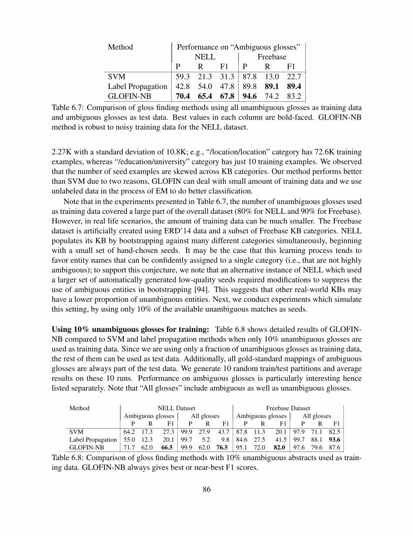
Method Performance on “Ambiguous glosses”NELL Freebase

P R F1 P R F1SVM 59.3 21.3 31.3 87.8 13.0 22.7Label Propagation 42.8 54.0 47.8 89.8 89.1 89.4GLOFIN-NB 70.4 65.4 67.8 94.6 74.2 83.2

Table 6.7: Comparison of gloss finding methods using all unambiguous glosses as training dataand ambiguous glosses as test data. Best values in each column are bold-faced. GLOFIN-NBmethod is robust to noisy training data for the NELL dataset.

2.27K with a standard deviation of 10.8K; e.g., “/location/location” category has 72.6K trainingexamples, whereas “/education/university” category has just 10 training examples. We observedthat the number of seed examples are skewed across KB categories. Our method performs betterthan SVM due to two reasons, GLOFIN can deal with small amount of training data and we useunlabeled data in the process of EM to do better classification.

Note that in the experiments presented in Table 6.7, the number of unambiguous glosses usedas training data covered a large part of the overall dataset (80% for NELL and 90% for Freebase).However, in real life scenarios, the amount of training data can be much smaller. The Freebasedataset is artificially created using ERD’14 data and a subset of Freebase KB categories. NELLpopulates its KB by bootstrapping against many different categories simultaneously, beginningwith a small set of hand-chosen seeds. It may be the case that this learning process tends tofavor entity names that can be confidently assigned to a single category (i.e., that are not highlyambiguous); to support this conjecture, we note that an alternative instance of NELL which useda larger set of automatically generated low-quality seeds required modifications to suppress theuse of ambiguous entities in bootstrapping [94]. This suggests that other real-world KBs mayhave a lower proportion of unambiguous entities. Next, we conduct experiments which simulatethis setting, by using only 10% of the available unambiguous matches as seeds.

Using 10% unambiguous glosses for training: Table 6.8 shows detailed results of GLOFIN-NB compared to SVM and label propagation methods when only 10% unambiguous glosses areused as training data. Since we are using only a fraction of unambiguous glosses as training data,the rest of them can be used as test data. Additionally, all gold-standard mappings of ambiguousglosses are always part of the test data. We generate 10 random train/test partitions and averageresults on these 10 runs. Performance on ambiguous glosses is particularly interesting hencelisted separately. Note that “All glosses” include ambiguous as well as unambiguous glosses.

Method NELL Dataset Freebase DatasetAmbiguous glosses All glosses Ambiguous glosses All glosses

P R F1 P R F1 P R F1 P R F1SVM 64.2 17.3 27.3 99.9 27.9 43.7 87.8 11.3 20.1 97.9 71.1 82.5Label Propagation 55.0 12.3 20.1 99.7 5.2 9.8 84.6 27.5 41.5 99.7 88.1 93.6GLOFIN-NB 71.7 62.0 66.5 99.9 62.0 76.5 95.1 72.0 82.0 97.6 79.6 87.6

Table 6.8: Comparison of gloss finding methods with 10% unambiguous abstracts used as train-ing data. GLOFIN-NB always gives best or near-best F1 scores.

86

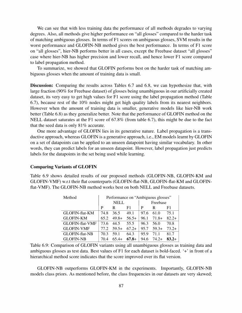
We can see that with less training data the performance of all methods degrades to varyingdegrees. Also, all methods give higher performance on “all glosses” compared to the harder taskof matching ambiguous glosses. In terms of F1 scores on ambiguous glosses, SVM results in theworst performance and GLOFIN-NB method gives the best performance. In terms of F1 scoreon “all glosses”, hier-NB performs better in all cases, except the Freebase dataset “all glosses”case where hier-NB has higher precision and lower recall, and hence lower F1 score comparedto label propagation method.

To summarize, we showed that GLOFIN performs best on the harder task of matching am-biguous glosses when the amount of training data is small.

Discussion: Comparing the results across Tables 6.7 and 6.8, we can hypothesize that, withlarge fraction (90% for Freebase dataset) of glosses being unambiguous in our artificially createddataset, its very easy to get high values for F1 score using the label propagation method (Table6.7), because rest of the 10% nodes might get high quality labels from its nearest neighbors.However when the amount of training data is smaller, generative models like hier-NB workbetter (Table 6.8) as they generalize better. Note that the performance of GLOFIN method on theNELL dataset saturates at the F1 score of 67.8% (from table 6.7), this might be due to the factthat the seed data is only 81% accurate.

One more advantage of GLOFIN lies in its generative nature. Label propagation is a trans-ductive approach, whereas GLOFIN is a generative approach, i.e., EM models learnt by GLOFINon a set of datapoints can be applied to an unseen datapoint having similar vocabulary. In otherwords, they can predict labels for an unseen datapoint. However, label propagation just predictslabels for the datapoints in the set being used while learning.

Comparing Variants of GLOFIN

Table 6.9 shows detailed results of our proposed methods (GLOFIN-NB, GLOFIN-KM andGLOFIN-VMF) w.r.t their flat counterparts (GLOFIN-flat-NB, GLOFIN-flat-KM and GLOFIN-flat-VMF). The GLOFIN-NB method works best on both NELL and Freebase datasets.

Method Performance on “Ambiguous glosses”NELL Freebase

P R F1 P R F1GLOFIN-flat-KM 74.8 36.5 49.1 97.6 61.0 75.1GLOFIN-KM 65.2 49.8+ 56.5+ 96.1 71.8+ 82.2+GLOFIN-flat-VMF 73.6 44.5 55.5 96.3 56.0 70.8GLOFIN-VMF 77.2 59.5+ 67.2+ 95.7 59.3+ 73.2+GLOFIN-flat-NB 70.3 59.1 64.3 95.9 71.1 81.7GLOFIN-NB 70.4 65.4+ 67.8+ 94.6 74.2+ 83.2+

Table 6.9: Comparison of GLOFIN variants using all unambiguous glosses as training data andambiguous glosses as test data. Best values of F1 for each dataset is bold-faced. ‘+’ in front of ahierarchical method score indicates that the score improved over its flat version.

GLOFIN-NB outperforms GLOFIN-KM in the experiments. Importantly, GLOFIN-NBmodels class priors. As mentioned before, the class frequencies in our datasets are very skewed;

87

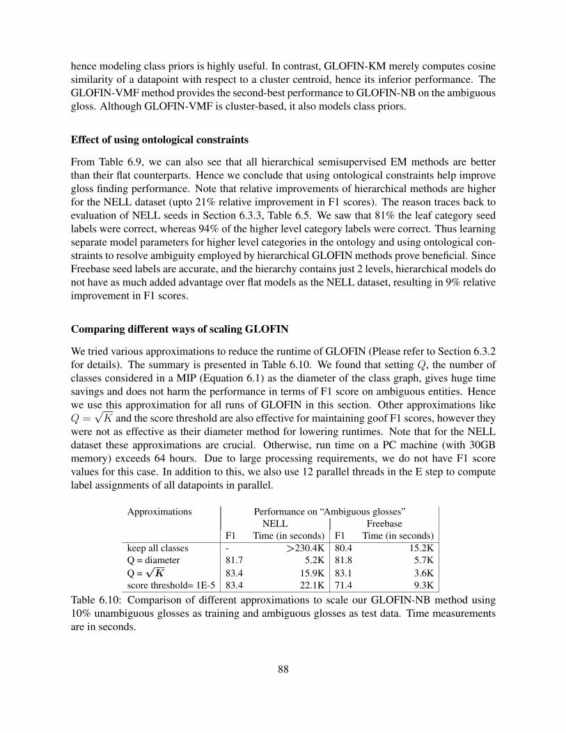
hence modeling class priors is highly useful. In contrast, GLOFIN-KM merely computes cosinesimilarity of a datapoint with respect to a cluster centroid, hence its inferior performance. TheGLOFIN-VMF method provides the second-best performance to GLOFIN-NB on the ambiguousgloss. Although GLOFIN-VMF is cluster-based, it also models class priors.

Effect of using ontological constraints

From Table 6.9, we can also see that all hierarchical semisupervised EM methods are betterthan their flat counterparts. Hence we conclude that using ontological constraints help improvegloss finding performance. Note that relative improvements of hierarchical methods are higherfor the NELL dataset (upto 21% relative improvement in F1 scores). The reason traces back toevaluation of NELL seeds in Section 6.3.3, Table 6.5. We saw that 81% the leaf category seedlabels were correct, whereas 94% of the higher level category labels were correct. Thus learningseparate model parameters for higher level categories in the ontology and using ontological con-straints to resolve ambiguity employed by hierarchical GLOFIN methods prove beneficial. SinceFreebase seed labels are accurate, and the hierarchy contains just 2 levels, hierarchical models donot have as much added advantage over flat models as the NELL dataset, resulting in 9% relativeimprovement in F1 scores.

Comparing different ways of scaling GLOFIN

We tried various approximations to reduce the runtime of GLOFIN (Please refer to Section 6.3.2for details). The summary is presented in Table 6.10. We found that setting Q, the number ofclasses considered in a MIP (Equation 6.1) as the diameter of the class graph, gives huge timesavings and does not harm the performance in terms of F1 score on ambiguous entities. Hencewe use this approximation for all runs of GLOFIN in this section. Other approximations likeQ =

√K and the score threshold are also effective for maintaining goof F1 scores, however they

were not as effective as their diameter method for lowering runtimes. Note that for the NELLdataset these approximations are crucial. Otherwise, run time on a PC machine (with 30GBmemory) exceeds 64 hours. Due to large processing requirements, we do not have F1 scorevalues for this case. In addition to this, we also use 12 parallel threads in the E step to computelabel assignments of all datapoints in parallel.

Approximations Performance on “Ambiguous glosses”NELL Freebase

F1 Time (in seconds) F1 Time (in seconds)keep all classes - >230.4K 80.4 15.2KQ = diameter 81.7 5.2K 81.8 5.7KQ =√K 83.4 15.9K 83.1 3.6K

score threshold= 1E-5 83.4 22.1K 71.4 9.3KTable 6.10: Comparison of different approximations to scale our GLOFIN-NB method using10% unambiguous glosses as training and ambiguous glosses as test data. Time measurementsare in seconds.

88

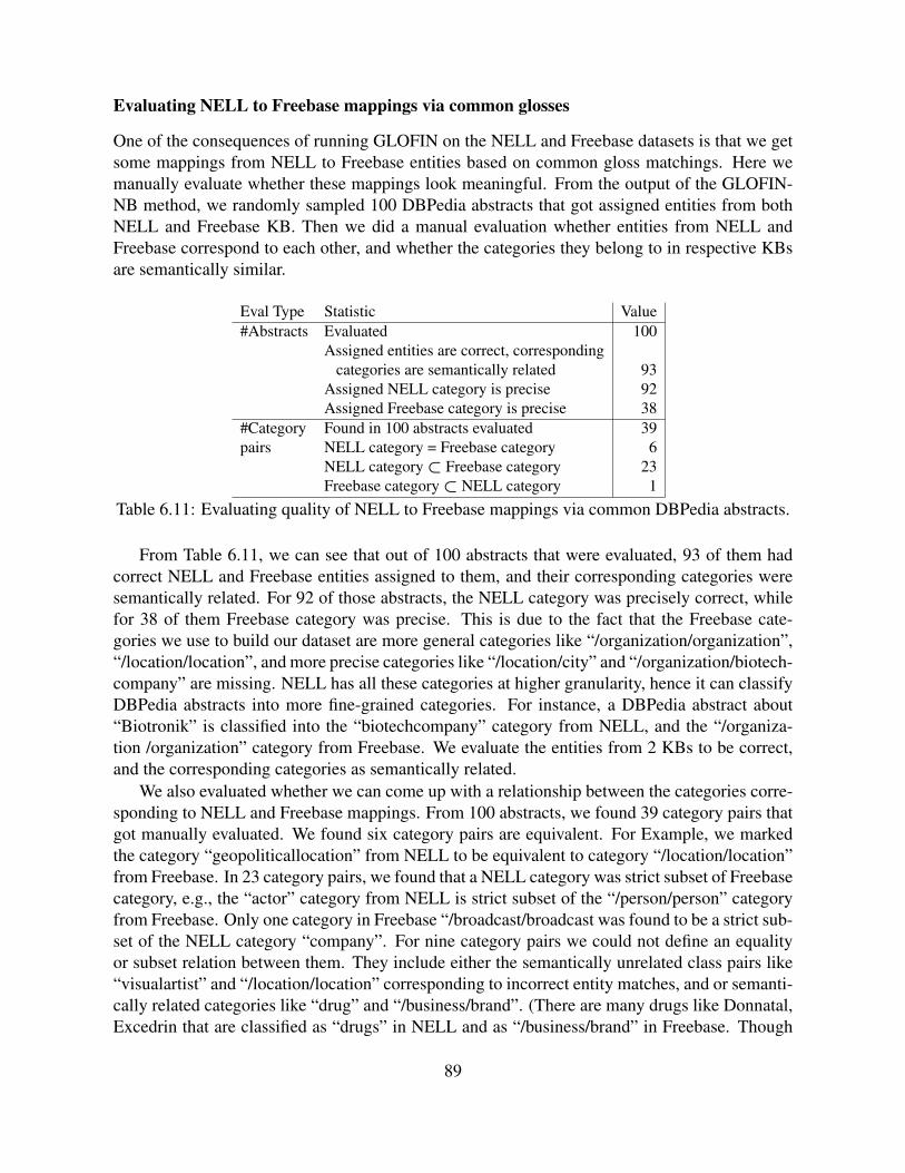
Evaluating NELL to Freebase mappings via common glosses

One of the consequences of running GLOFIN on the NELL and Freebase datasets is that we getsome mappings from NELL to Freebase entities based on common gloss matchings. Here wemanually evaluate whether these mappings look meaningful. From the output of the GLOFIN-NB method, we randomly sampled 100 DBPedia abstracts that got assigned entities from bothNELL and Freebase KB. Then we did a manual evaluation whether entities from NELL andFreebase correspond to each other, and whether the categories they belong to in respective KBsare semantically similar.

Eval Type Statistic Value#Abstracts Evaluated 100

Assigned entities are correct, correspondingcategories are semantically related 93

Assigned NELL category is precise 92Assigned Freebase category is precise 38

#Category Found in 100 abstracts evaluated 39pairs NELL category = Freebase category 6

NELL category⊂ Freebase category 23Freebase category⊂ NELL category 1

Table 6.11: Evaluating quality of NELL to Freebase mappings via common DBPedia abstracts.

From Table 6.11, we can see that out of 100 abstracts that were evaluated, 93 of them hadcorrect NELL and Freebase entities assigned to them, and their corresponding categories weresemantically related. For 92 of those abstracts, the NELL category was precisely correct, whilefor 38 of them Freebase category was precise. This is due to the fact that the Freebase cate-gories we use to build our dataset are more general categories like “/organization/organization”,“/location/location”, and more precise categories like “/location/city” and “/organization/biotech-company” are missing. NELL has all these categories at higher granularity, hence it can classifyDBPedia abstracts into more fine-grained categories. For instance, a DBPedia abstract about“Biotronik” is classified into the “biotechcompany” category from NELL, and the “/organiza-tion /organization” category from Freebase. We evaluate the entities from 2 KBs to be correct,and the corresponding categories as semantically related.

We also evaluated whether we can come up with a relationship between the categories corre-sponding to NELL and Freebase mappings. From 100 abstracts, we found 39 category pairs thatgot manually evaluated. We found six category pairs are equivalent. For Example, we markedthe category “geopoliticallocation” from NELL to be equivalent to category “/location/location”from Freebase. In 23 category pairs, we found that a NELL category was strict subset of Freebasecategory, e.g., the “actor” category from NELL is strict subset of the “/person/person” categoryfrom Freebase. Only one category in Freebase “/broadcast/broadcast was found to be a strict sub-set of the NELL category “company”. For nine category pairs we could not define an equalityor subset relation between them. They include either the semantically unrelated class pairs like“visualartist” and “/location/location” corresponding to incorrect entity matches, and or semanti-cally related categories like “drug” and “/business/brand”. (There are many drugs like Donnatal,Excedrin that are classified as “drugs” in NELL and as “/business/brand” in Freebase. Though

89

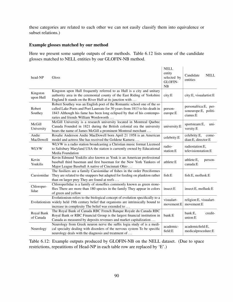
these categories are related to each other we can not easily classify them into equivalence orsubset relations.)

Example glosses matched by our method

Here we present some sample outputs of our methods. Table 6.12 lists some of the candidateglosses matched to NELL entities by our GLOFIN-NB method.

head-NP Gloss

NELLentityselected byGLOFIN-NB

Candidate NELLentities

Kingstonupon Hull

Kingston upon Hull frequently referred to as Hull is a city and unitaryauthority area in the ceremonial county of the East Riding of YorkshireEngland It stands on the River Hull at its junction with . . .

city:E city:E, visualartist:E

RobertSouthey

Robert Southey was an English poet of the Romantic school one of the socalled Lake Poets and Poet Laureate for 30 years from 1813 to his death in1843 Although his fame has been long eclipsed by that of his contempo-raries and friends William Wordsworth . . .

person-europe:E

personafrica:E, per-soneurope:E, politi-cianus:E

McGillUniversity

McGill University is a research university located in Montreal QuebecCanada Founded in 1821 during the British colonial era the universitybears the name of James McGill a prominent Montreal merchant . . .

university:Esportsteam:E, uni-versity:E

AndieMacDowell

Rosalie Anderson Andie MacDowell born April 21 1958 is an Americanmodel and actress She has received the Goldene Kamera . . .

celebrity:Ecelebrity:E, come-dian:E, director:E

WLVWWLVW is a radio station broadcasting a Christian music format Licensedto Salisbury Maryland USA the station is currently owned by EducationalMedia Foundation

radio-station:E

radiostation:E,televisionstation:E

KevinYoukilis

Kevin Edmund Youkilis also known as Youk is an American professionalbaseball third baseman and first baseman for the New York Yankees ofMajor League Baseball A native of Cincinnati Ohio . . .

athlete:Eathlete:E, person-canada:E

CaesionidaeThe fusiliers are a family Caesionidae of fishes in the order PerciformesThey are related to the snappers but adapted for feeding on plankton ratherthan on larger prey They are found at reefs . . .

fish:E fish:E, mollusk:E

Chloroper-lidae

Chloroperlidae is a family of stoneflies commonly known as green stone-flies There are more than 180 species in the family They appear in colorsof green and yellow

insect:E insect:E, mollusk:E

EvolutionismEvolutionism refers to the biological concept of evolution specifically to awidely held 19th century belief that organisms are intrinsically bound toincrease in complexity The belief was extended to . . .

visualart-movement:E

religion:E, visualart-movement:E

Royal Bankof Canada

The Royal Bank of Canada RBC French Banque Royale du Canada RBCRoyal Bank or RBC Financial Group is the largest financial institution inCanada as measured by deposits revenues and market capitalization . . .

bank:Ebank:E, credit-union:E

NeurologyNeurology from Greek neuron nerve the suffix logia study of is a medi-cal specialty dealing with disorders of the nervous system To be specificneurology deals with the diagnosis and treatment of . . .

academic-field:E

academicfield:E,medicalprocedure:E

Table 6.12: Example outputs produced by GLOFIN-NB on the NELL dataset. (Due to spacerestrictions, repeatitions of Head-NP in each table row are replaced by ‘E’.)

90

6.4 Related Work

6.4.1 Hierarchical Semi-supervised LearningThere has been some work on modifying EM to incorporate side information such as multi-view constraints or domain knowledge based constraints on outputs. The posterior regularizationframework [49] modifies the EM algorithm to encode domain constraints on the expected out-put, which has also been extended to incorporate soft agreement in a multi-view setting [50]. Ourtechnique Hier-MAXAGREE is different in that it maximizes agreement between the labels pro-duced in each view while satisfying ontological class constraints if available, whereas the methodproposed by Ganchev et al. [50] minimizes the difference between actual scores produced by theviews.

Chang et al. [29] proposed an extension of EM algorithm for encoding the task specificdomain knowledge base constraints on the output. Our hierarchical techniques are similar tothis in the sense that we also modify the EM algorithm to do constrained learning. Howeverour techniques are different from [29] in the sense we are using constraints specific to a dataset:e.g., for the NELL mv dataset, the ontological constraints we used are the same as the oneswhich were used while building the NELL knowledge base. We did not need any hand curatedconstraints for the specific task that we worked on. Further we take care of the agreement acrossviews and ontological constraints in a single framework using multiple soft constraints.

Graph based multi-view semisupervised learning techniques have also been proposed in pastfew years. Wang et al. [135] proposed a multi-graph based semisupervised learning techniquethat can incorporate multiple modalities, and multiple distance functions in the task of videoannotation. Lee et al. [75] proposed a new graph-based multi-label propagation technique andapplied it to large datasets by utilizing a map-reduce framework. Though these methods canhandle multi-view data, they fail to address the scenarios where classes/labels are arranged in ahierarchy and inference needs to be done following certain constraints between these classes.

Here we propose a mixed integer programming based optimization method that can deal withany class hierarchy defined by sets of subset and mutual exclusion constraints. Interestingly, arecent work has used mixed integer LP techniques to encode ontological constraints [95]–theyassign multiple plausible KB categories to ‘emerging’ entities, which are not yet represented inthe KB, and consider mutual exclusion constraints as a post-processing step, so as to output aconsistent set of category assignments. In contrast, we apply subset as well as mutual exclusionconstraints, within an iterative EM algorithm, using semi-supervised learning Finally, while theapplication of earlier variants of the EM-based framework focused on the named entity catego-rization task, we use the proposed methods for addressing the novel task of generating glossesfor an existing KB.

6.4.2 Gloss FindingGlosses are an important resource of word meanings, which has been used by word sense dis-ambiguation (WSD) [96] algorithms for decades. For example, the popular Lesk method [77]and its variants [8, 71] infer a word’s sense by measuring the overlap between available contextwords and the glosses of candidate senses. Traditionally, WordNet [46] has been used as the

91

main resource of word senses and respective glosses. Several recent works have investigated theproblem of automatic gloss extraction, so as to improve coverage in specific knowledge domains.Duan and Yates [39] constructed sense descriptions for selected keywords given unlabeled doc-uments in the Biomedical domain, and used these descriptions to perform WSD. Others [36, 44]constructed domain-specific glossaries using definitional sentences extracted from the Web, andsuccessfully used these glossaries for domain WSD. We share their motivation for obtainingglosses, however rather than generate these glosses, our goal is to associate available glosseswith an existing KB.

We match given glosses against the respective entity nodes in the KB. This task is closelyrelated to Entity Linking (EL), an entity-focused variant of the WSD problem [93], where namedentity mentions in a given text are linked with the respective nodes in a KB. Advanced EL meth-ods consider multiple entity mentions in a document collectively in order to enrich the contextualinformation that is modeled per entity [58, 134]. Such methods are ineffective for short text frag-ments, like search queries, or glosses. In fact, we face a ‘chicken and egg’ problem, as mostEL methods assume that KB entities have glosses, whereas we do not [60, 80]. Here, we areinterested in enriching a KB with glosses, so as to support entity linking and other downstreamapplications, such as ad-hoc information retrieval [34, 143].

Various works have addressed the problem of resource alignment, but considered differentsettings. The Yago ontology [118], for example, unifies Wikipedia and WordNet using heuris-tics that consider the structure of both resources. Ponzetto and Navigli [105] mapped Wikipediaarticles onto WordNet synsets, using the textual descriptions of entity pairs. We rather consideran asymmetric setting, where the KB includes a semantic structure but lacks textual descrip-tions, and the aligned glosses are not assumed to be organized in any fashion. Similarly, arecent work [104] addressed the alignment of an arbitrary pair of lexical resources, includingmachine-readable dictionaries with no structure. They proposed to induce a network structurefor dictionary resources, however textual similarity remains an important component in their ap-proach. Importantly, having enriched a given KB with glosses using the proposed framework,this will facilitate its alignment and integration with other KBs [32].

We addressed the gloss finding problem using a semi-supervised framework. In particular,we consider label propagation (LP), where gloss nodes are being associated with candidate en-tity nodes based on their relatedness in a joint graph. Talukdar [119] discuss the use of weaklysupervised label propagation methods in information extraction and integration. Previous workapplied LP to perform WSD [146]. In that case, the graph modeled words in parallel documentsin two languages, where word ambiguity in one language was resolved based on graph related-ness to their candidate translation in the other language, and vice versa. The use of graph-basedmethods is highly prevalent in WSD literature. In particular, random walks over a semanticgraph, like WordNet, have shown to yield state-of-the-art results [4, 105]. Notably, linking nodesin the WordNet graph based on lexical gloss overlaps has been shown to contribute significantlyto the performance of graph-based WSD [4].

92

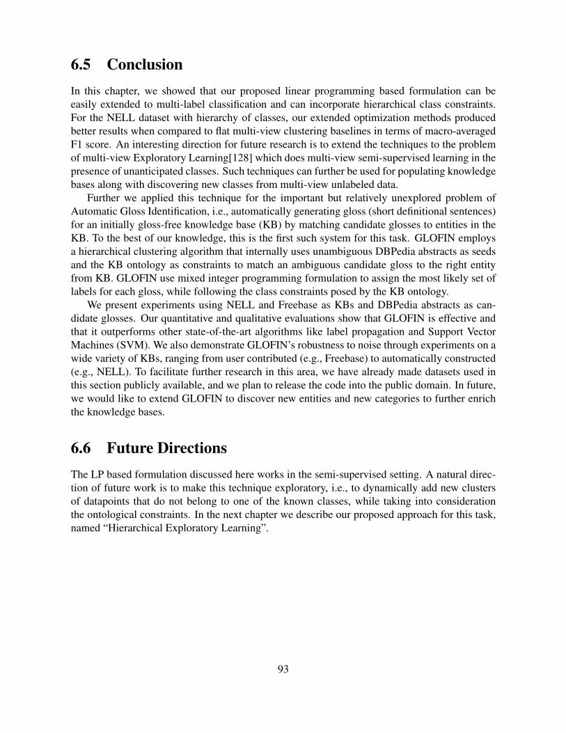
6.5 ConclusionIn this chapter, we showed that our proposed linear programming based formulation can beeasily extended to multi-label classification and can incorporate hierarchical class constraints.For the NELL dataset with hierarchy of classes, our extended optimization methods producedbetter results when compared to flat multi-view clustering baselines in terms of macro-averagedF1 score. An interesting direction for future research is to extend the techniques to the problemof multi-view Exploratory Learning[128] which does multi-view semi-supervised learning in thepresence of unanticipated classes. Such techniques can further be used for populating knowledgebases along with discovering new classes from multi-view unlabeled data.

Further we applied this technique for the important but relatively unexplored problem ofAutomatic Gloss Identification, i.e., automatically generating gloss (short definitional sentences)for an initially gloss-free knowledge base (KB) by matching candidate glosses to entities in theKB. To the best of our knowledge, this is the first such system for this task. GLOFIN employsa hierarchical clustering algorithm that internally uses unambiguous DBPedia abstracts as seedsand the KB ontology as constraints to match an ambiguous candidate gloss to the right entityfrom KB. GLOFIN use mixed integer programming formulation to assign the most likely set oflabels for each gloss, while following the class constraints posed by the KB ontology.

We present experiments using NELL and Freebase as KBs and DBPedia abstracts as can-didate glosses. Our quantitative and qualitative evaluations show that GLOFIN is effective andthat it outperforms other state-of-the-art algorithms like label propagation and Support VectorMachines (SVM). We also demonstrate GLOFIN’s robustness to noise through experiments on awide variety of KBs, ranging from user contributed (e.g., Freebase) to automatically constructed(e.g., NELL). To facilitate further research in this area, we have already made datasets used inthis section publicly available, and we plan to release the code into the public domain. In future,we would like to extend GLOFIN to discover new entities and new categories to further enrichthe knowledge bases.

6.6 Future DirectionsThe LP based formulation discussed here works in the semi-supervised setting. A natural direc-tion of future work is to make this technique exploratory, i.e., to dynamically add new clustersof datapoints that do not belong to one of the known classes, while taking into considerationthe ontological constraints. In the next chapter we describe our proposed approach for this task,named “Hierarchical Exploratory Learning”.

93

94

Chapter 7

Exploratory Learning with An IncompleteClass Ontology

In an open-domain entity classification task, topic or concept hierarchies are often incomplete. InChapter 4 we showed that in a non-hierarchical semi-supervised classification task, the presenceof such unanticipated classes can cause semantic drift for seeded classes. Exploratory learning[128] method was proposed to solve this problem by exploring a different number of classeswhile learning classifiers for each of them. However it is limited to the flat classification task.This chapter extends the Exploratory learning method to hierarchical classification tasks. Thiswork is partially published in the proceedings of AKBC 2013 [127] and the remaining work isunder preparation for submission [124].

We experimented with subsets of the NELL [25] ontology and text, and HTML table datasetsderived from the ClueWeb09 corpus. Our method OptDAC-ExploreEM improves seed classF1 on average by 13% when compared to its semi-supervised counterpart (OptDAC). It alsooutperforms both previously proposed exploratory learning approaches FLAT-ExploreEM andDAC-ExploreEM [127] in terms of seed class F1 on average by 10% and 7% respectively.

7.1 Motivation

A common way to organize information is by classification into a concept or topic hierarchy. TheOpen Directory Project and the Yahoo! Directory are examples of topic hierarchies developed toorganize pages on the Web. Wordnet, NELL and Freebase are examples of large knowledge basesthat organize entities into concept hierarchies. However, in an open-domain task, hierarchiesare often incomplete, in the sense that there is meaningful structure in the data not capturedby the existing hierarchy. For example, consider a hierarchical entity classification task, withclass hierarchy ‘onto-1’ shown in Figure 7.1 (left). There are 2 types of locations defined init: ‘State’ and ‘Country’. However, the unlabeled data about entities on the Web can includelocation entities of type ‘City’, ‘Museum’ etc. , that are absent in this ontology, hence called‘unanticipated classes’.

In Chapter 4 we showed that in a non-hierarchical semi-supervised classification task, thepresence of such unanticipated classes hidden in the unlabeled data can cause semantic drift for

95

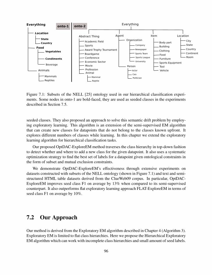
Figure 7.1: Subsets of the NELL [25] ontology used in our hierarchical classification experi-ments. Some nodes in onto-1 are bold-faced, they are used as seeded classes in the experimentsdescribed in Section 7.5.

seeded classes. They also proposed an approach to solve this semantic drift problem by employ-ing exploratory learning. This algorithm is an extension of the semi-supervised EM algorithmthat can create new classes for datapoints that do not belong to the classes known upfront. Itexplores different numbers of classes while learning. In this chapter we extend the exploratorylearning algorithm for hierarchical classification tasks.

Our proposed OptDAC-ExploreEM method traverses the class hierarchy in top-down fashionto detect whether and where to add a new class for the given datapoint. It also uses a systematicoptimization strategy to find the best set of labels for a datapoint given ontological constraints inthe form of subset and mutual exclusion constraints.

We demonstrate OptDAC-ExploreEM’s effectiveness through extensive experiments ondatasets constructed with subsets of the NELL ontology (shown in Figure 7.1) and text and semi-structured HTML table datasets derived from the ClueWeb09 corpus. In particular, OptDAC-ExploreEM improves seed class F1 on average by 13% when compared to its semi-supervisedcounterpart. It also outperforms flat exploratory learning approach FLAT-ExploreEM in terms ofseed class F1 on average by 10%.

7.2 Our Approach

Our method is derived from the Exploratory EM algorithm described in Chapter 4 (Algorithm 3).Exploratory EM is limited to flat class hierarchies. Here we propose the Hierarchical ExploratoryEM algorithm which can work with incomplete class hierarchies and small amount of seed labels.

96

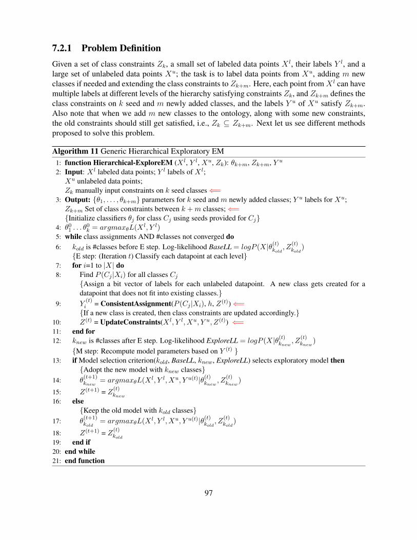
7.2.1 Problem DefinitionGiven a set of class constraints Zk, a small set of labeled data points X l, their labels Y l, and alarge set of unlabeled data points Xu; the task is to label data points from Xu, adding m newclasses if needed and extending the class constraints to Zk+m. Here, each point fromX l can havemultiple labels at different levels of the hierarchy satisfying constraints Zk, and Zk+m defines theclass constraints on k seed and m newly added classes, and the labels Y u of Xu satisfy Zk+m.Also note that when we add m new classes to the ontology, along with some new constraints,the old constraints should still get satisfied, i.e., Zk ⊆ Zk+m. Next let us see different methodsproposed to solve this problem.

Algorithm 11 Generic Hierarchical Exploratory EM1: function Hierarchical-ExploreEM (X l, Y l, Xu, Zk): θk+m, Zk+m, Y u

2: Input: X l labeled data points; Y l labels of X l;Xu unlabeled data points;Zk manually input constraints on k seed classes⇐=

3: Output: θ1, . . . , θk+m parameters for k seed and m newly added classes; Y u labels for Xu;Zk+m Set of class constraints between k +m classes;⇐=Initialize classifiers θj for class Cj using seeds provided for Cj

4: θ01 . . . θ

0k = argmaxθL(X

l, Y l)5: while class assignments AND #classes not converged do6: kold is #classes before E step. Log-likelihood BaseLL = logP (X|θ(t)

kold, Z

(t)kold

)E step: (Iteration t) Classify each datapoint at each level

7: for i=1 to |X| do8: Find P (Cj |Xi) for all classes Cj

Assign a bit vector of labels for each unlabeled datapoint. A new class gets created for adatapoint that does not fit into existing classes.

9: Y(t)i = ConsistentAssignment(P (Cj |Xi), h, Z(t))⇐=If a new class is created, then class constraints are updated accordingly.

10: Z(t) = UpdateConstraints(X l, Y l, Xu, Y u, Z(t)) ⇐=11: end for12: knew is #classes after E step. Log-likelihood ExploreLL = logP (X|θ(t)

knew, Z

(t)knew

)

M step: Recompute model parameters based on Y (t) 13: if Model selection criterion(kold, BaseLL, knew, ExploreLL) selects exploratory model then

Adopt the new model with knew classes14: θ

(t+1)knew

= argmaxθL(Xl, Y l, Xu, Y u(t)|θ(t)

knew, Z

(t)knew

)

15: Z(t+1) = Z(t)knew

16: elseKeep the old model with kold classes

17: θ(t+1)kold

= argmaxθL(Xl, Y l, Xu, Y u(t)|θ(t)

kold, Z

(t)kold

)

18: Z(t+1) = Z(t)kold

19: end if20: end while21: end function

97

7.2.2 Flat Exploratory EM

One simple way to use Exploratory EM algorithm [128] for our purpose will be to run it as it is ateach level of hierarchy. Henceforth, we refer to this approach as FLAT-ExploreEM and considerit as a baseline for our proposed Hierarchical Exploratory EM approach. At each level, it selectsone of the existing classes or creates a new class in case the datapoint doesn’t clearly belong toone of the known classes. This algorithm does not make explicit use of class constraints whilemaking class assignments at each step. Hence the assignments done by this algorithm might notbe consistent, since assignments at level 3 are not influenced by assignment at level 2.

7.2.3 Hierarchical Exploratory EM

We propose a generic Hierarchical exploratory learning algorithm that can take a set of classconstraints in terms of subclass or mutual exclusion constraints. This algorithm, in each iteration,assigns a bit vector to each data point with one bit per class. Class constraints decide whethera bit vector is consistent or not, e.g., if class constraints include “Car is of type Machine”, thenfor consistency, when the bit for “Car” is set, the bit for “Machine” should also be set. Furthernew classes can be added during each iteration, hence the length of these bit vectors changesdynamically and the algorithm maintains class constraints containing old as well as newly addedclasses. The generic algorithm is described in Algorithm 11. There can be multiple ways toimplement functions “ConsistentAssignment” and “UpdateConstraints”.

Lines 13-19 of Algorithm 11 do model selection. Similar to Exploratory EM [128], at theend of every E step, we evaluate two models, one with and one without adding extra classes.These two models are scored using a model selection criterion like AIC, BIC or AICc, andthe model with best penalized data likelihood score is selected in each iteration. The extendedAkaike information criterion (AICc) suited best for our experiments since our datasets have largenumber of features and small number of data points. The class constraints are modeled in thesame way as described in Section 6.1.1.

7.3 Variants of Hierarchical Exploratory EM

Hierarchical Exploratory EM (described in Algorithm 11) is a generic algorithm that can beinstantiated in different ways, by changing the functions “ConsistentAssignment” and “Up-dateConstraints”. Next we describe two such variants namely, DAC-ExploreEM and OptDAC-ExploreEM.

7.3.1 Divide and Conquer (DAC-ExploreEM)

One simple instantiation of Algorithm 11 can be done by using Divide-and-Conquer (DAC)strategy introduced in [127]. Here we assume that classes are arranged in a tree hierarchy, andclasses at any one level are mutually exclusive. To do class assignments for any unlabeled data-point, we traverse the class ontology from root to leaf level. Every data point belongs to the root

98

node. Then at each level we chose the best label at that level and consider only its children ascandidates at the next level.

Further we check whether the probability distribution among the candidate classes at eachlevel is nearly uniform (using heuristic described in Algorithm 5) to decide whether to createa new class at that level. We do not describe the “ConsistentAssignment” and “UpdateCon-straints” functions formally, however they can be easily derived by setting parameter q = 1 inthe OptDAC-ExploreEM algorithm that we present next.

DAC-ExploreEMcan do semi-supervised learning if the presence of unanticipated classes.However, we will see in the experimental evaluation (refer to Section 7.5.2) that DAC-ExploreEM could provide marginal improvements over the baseline (Exploratory EM). Duringthe error analysis we found that the classification at higher levels of hierarchy is not perfect, andonce we make a decision at level i of the ontology, there is no way to change the decision oncewe move on to level i+1. Next we try a softer version of this method, that keeps track of q nodesat each level instead of keeping only the best label.

Also, note that the example ontologies in Figure 7.1 have tree structure. However, in prac-tice, class constraints can be more complicated (e.g., overlapping classes can exist). The DAC-ExploreEM algorithm is limited to a tree structured ontology and assumes mutual exclusion ofclasses at any level of hierarchy. Next we present the OptDAC-ExploreEM algorithm that canwork with more complicated class constraints.

7.3.2 Optimized Divide and Conquer (OptDAC-ExploreEM)Algorithm 12 describes how the “ConsistentAssignment” and “UpdateConstraints” functions areimplemented for this approach. It is similar to DAC-ExploreEM method in the sense that wetraverse the classes in top down fashion, and check whether new class needs to be created at eachlevel of the hierarchy. However, at each level l of the class hierarchy, a mixed-integer programis run to get optimal class assignments for the active classes from levels 1 to l. Further insteadof considering only the best class, top-q classes from each level are selected to be added intothe set of active classes which are used in turn to select the candidate classes at the next level ofhierarchy.

This method combines the Divide-and-Conquer strategy to detect/place new classes and themixed integer programming based optimization strategy to assign an optimal set of labels toa datapoint given the ontological constraints. The optimal label assignment method is genericenough to support any set of subset and mutual exclusion class constraints. The new class detec-tion based on Divide and Conquer can be extended for non-tree hierarchies using a breadth firstsearch strategy that can be applied to any graph. Hence the OptDAC-ExploreEM method can beextended easily for non-tree structured ontologies.

Note that similar to DAC-ExploreEM, it makes greedy decisions about new cluster creation.However, it performs overall optimization of label assignments while satisfying the ontologicalconstraints. This lets us correct any sub-optimal decisions made by the greedy heuristic at higherlevels of the class hierarchy. Further, as we increase the value of q, we might get some improve-ment in accuracy at the cost of increased runtime. Since the value of q directly decides the size ofactive nodes set used while taking the decision at each level of the hierarchy, there is a trade-offbetween time complexity and solution optimality. For all the experiments in this paper, we added

99

top two classes per level to the set of selected classes (i.e. q = 2) in Line 21 of Algorithm 12.This approach is referred to as OptDAC-ExploreEM below.

For each datapoint, the optimal label assignment given class constraints (Algorithm 12: Line24) if computed using Equation 6.1. To solve these mixed integer linear programs we used theMOSEK solver [5]. We have used such optimization techniques for the task of semi-supervisedlearning in the presence of multiple data views and hierarchical class constraints [123, 130]. Herewe use this formulation for the task of hierarchical exploratory learning.

100

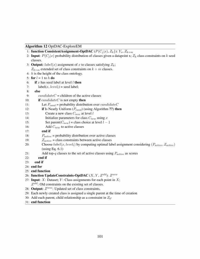
Algorithm 12 OptDAC-ExploreEM1: function ConsistentAssignment-OptDAC (P (Cj |x), Zk): Yx, Zk+m

2: Input: P (Cj |x) probability distribution of classes given a datapoint x; Zk class constraints on k seedclasses.

3: Output: label(x) assignment of x to classes satisfying Zk;Zk+m extended set of class constraints on k +m classes.

4: h is the height of the class ontology.5: for l = 1 to h do6: if x has seed label at level l then7: label(x, levell) = seed label;8: else9: candidateC = children of the active classes

10: if candidateC is not empty then11: Let Pcand = probability distribution over candidateC12: if Is Nearly Uniform (Pcand) (using Algorithm ??) then13: Create a new class Cnew at level l14: Initialize parameters for class Cnew using x15: Set parent(Cnew) = class choice at level l − 116: Add Cnew to active classes17: end if18: Pactive = probability distribution over active classes19: Zactive = class constraints between active classes20: Choose label(x, levell) by computing optimal label assignment considering (Pactive, Zactive)

(using Eq. 6.1)21: Add top-q classes to the set of active classes using Pactive as scores22: end if23: end if24: end for25: end function26: function UpdateConstraints-OptDAC (X , Y , Zold): Znew

27: Input: X: Dataset; Y : Class assignments for each point in X;Zold: Old constraints on the existing set of classes.

28: Output: Znew: Updated set of class constraints,29: Each newly created class is assigned a single parent at the time of creation30: Add each parent, child relationship as a constraint in Zk′31: end function

101

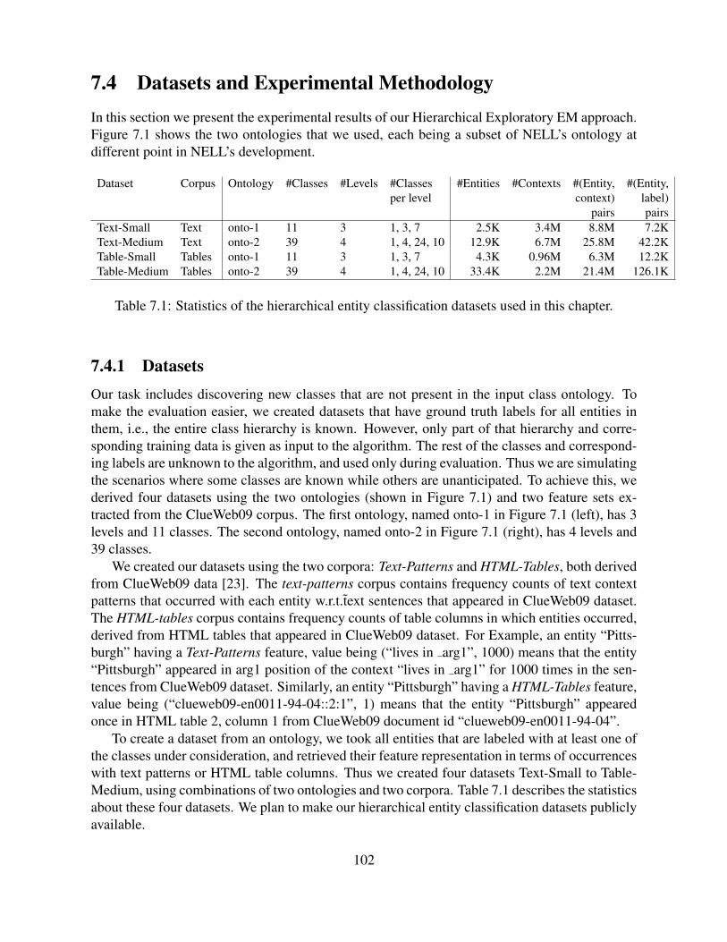
7.4 Datasets and Experimental MethodologyIn this section we present the experimental results of our Hierarchical Exploratory EM approach.Figure 7.1 shows the two ontologies that we used, each being a subset of NELL’s ontology atdifferent point in NELL’s development.

Dataset Corpus Ontology #Classes #Levels #Classes #Entities #Contexts #(Entity, #(Entity,per level context) label)

pairs pairsText-Small Text onto-1 11 3 1, 3, 7 2.5K 3.4M 8.8M 7.2KText-Medium Text onto-2 39 4 1, 4, 24, 10 12.9K 6.7M 25.8M 42.2KTable-Small Tables onto-1 11 3 1, 3, 7 4.3K 0.96M 6.3M 12.2KTable-Medium Tables onto-2 39 4 1, 4, 24, 10 33.4K 2.2M 21.4M 126.1K

Table 7.1: Statistics of the hierarchical entity classification datasets used in this chapter.

7.4.1 DatasetsOur task includes discovering new classes that are not present in the input class ontology. Tomake the evaluation easier, we created datasets that have ground truth labels for all entities inthem, i.e., the entire class hierarchy is known. However, only part of that hierarchy and corre-sponding training data is given as input to the algorithm. The rest of the classes and correspond-ing labels are unknown to the algorithm, and used only during evaluation. Thus we are simulatingthe scenarios where some classes are known while others are unanticipated. To achieve this, wederived four datasets using the two ontologies (shown in Figure 7.1) and two feature sets ex-tracted from the ClueWeb09 corpus. The first ontology, named onto-1 in Figure 7.1 (left), has 3levels and 11 classes. The second ontology, named onto-2 in Figure 7.1 (right), has 4 levels and39 classes.

We created our datasets using the two corpora: Text-Patterns and HTML-Tables, both derivedfrom ClueWeb09 data [23]. The text-patterns corpus contains frequency counts of text contextpatterns that occurred with each entity w.r.t.text sentences that appeared in ClueWeb09 dataset.The HTML-tables corpus contains frequency counts of table columns in which entities occurred,derived from HTML tables that appeared in ClueWeb09 dataset. For Example, an entity “Pitts-burgh” having a Text-Patterns feature, value being (“lives in arg1”, 1000) means that the entity“Pittsburgh” appeared in arg1 position of the context “lives in arg1” for 1000 times in the sen-tences from ClueWeb09 dataset. Similarly, an entity “Pittsburgh” having a HTML-Tables feature,value being (“clueweb09-en0011-94-04::2:1”, 1) means that the entity “Pittsburgh” appearedonce in HTML table 2, column 1 from ClueWeb09 document id “clueweb09-en0011-94-04”.

To create a dataset from an ontology, we took all entities that are labeled with at least one ofthe classes under consideration, and retrieved their feature representation in terms of occurrenceswith text patterns or HTML table columns. Thus we created four datasets Text-Small to Table-Medium, using combinations of two ontologies and two corpora. Table 7.1 describes the statisticsabout these four datasets. We plan to make our hierarchical entity classification datasets publiclyavailable.

102

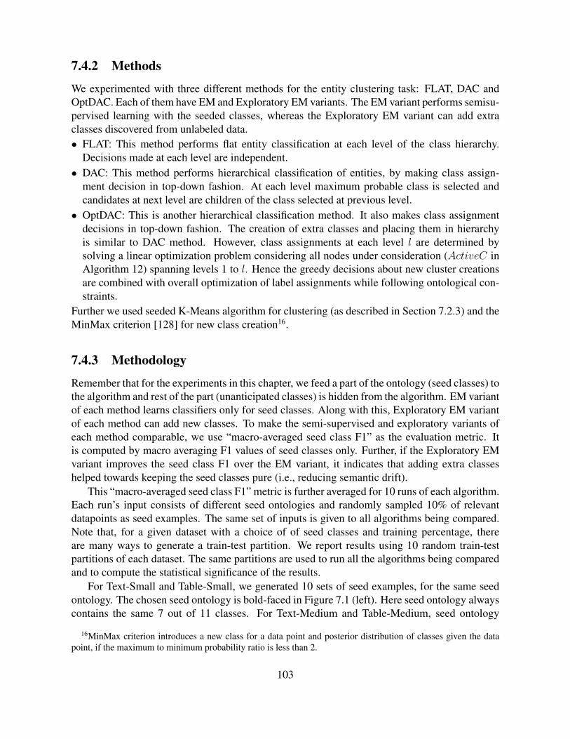
7.4.2 Methods

We experimented with three different methods for the entity clustering task: FLAT, DAC andOptDAC. Each of them have EM and Exploratory EM variants. The EM variant performs semisu-pervised learning with the seeded classes, whereas the Exploratory EM variant can add extraclasses discovered from unlabeled data.• FLAT: This method performs flat entity classification at each level of the class hierarchy.

Decisions made at each level are independent.• DAC: This method performs hierarchical classification of entities, by making class assign-

ment decision in top-down fashion. At each level maximum probable class is selected andcandidates at next level are children of the class selected at previous level.• OptDAC: This is another hierarchical classification method. It also makes class assignment

decisions in top-down fashion. The creation of extra classes and placing them in hierarchyis similar to DAC method. However, class assignments at each level l are determined bysolving a linear optimization problem considering all nodes under consideration (ActiveC inAlgorithm 12) spanning levels 1 to l. Hence the greedy decisions about new cluster creationsare combined with overall optimization of label assignments while following ontological con-straints.

Further we used seeded K-Means algorithm for clustering (as described in Section 7.2.3) and theMinMax criterion [128] for new class creation16.

7.4.3 Methodology

Remember that for the experiments in this chapter, we feed a part of the ontology (seed classes) tothe algorithm and rest of the part (unanticipated classes) is hidden from the algorithm. EM variantof each method learns classifiers only for seed classes. Along with this, Exploratory EM variantof each method can add new classes. To make the semi-supervised and exploratory variants ofeach method comparable, we use “macro-averaged seed class F1” as the evaluation metric. Itis computed by macro averaging F1 values of seed classes only. Further, if the Exploratory EMvariant improves the seed class F1 over the EM variant, it indicates that adding extra classeshelped towards keeping the seed classes pure (i.e., reducing semantic drift).

This “macro-averaged seed class F1” metric is further averaged for 10 runs of each algorithm.Each run’s input consists of different seed ontologies and randomly sampled 10% of relevantdatapoints as seed examples. The same set of inputs is given to all algorithms being compared.Note that, for a given dataset with a choice of of seed classes and training percentage, thereare many ways to generate a train-test partition. We report results using 10 random train-testpartitions of each dataset. The same partitions are used to run all the algorithms being comparedand to compute the statistical significance of the results.

For Text-Small and Table-Small, we generated 10 sets of seed examples, for the same seedontology. The chosen seed ontology is bold-faced in Figure 7.1 (left). Here seed ontology alwayscontains the same 7 out of 11 classes. For Text-Medium and Table-Medium, seed ontology

16MinMax criterion introduces a new class for a data point and posterior distribution of classes given the datapoint, if the maximum to minimum probability ratio is less than 2.

103

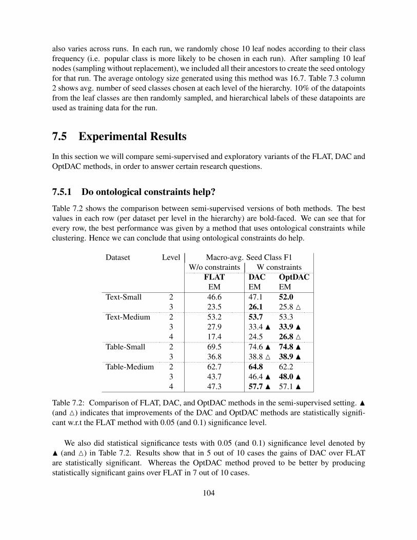
also varies across runs. In each run, we randomly chose 10 leaf nodes according to their classfrequency (i.e. popular class is more likely to be chosen in each run). After sampling 10 leafnodes (sampling without replacement), we included all their ancestors to create the seed ontologyfor that run. The average ontology size generated using this method was 16.7. Table 7.3 column2 shows avg. number of seed classes chosen at each level of the hierarchy. 10% of the datapointsfrom the leaf classes are then randomly sampled, and hierarchical labels of these datapoints areused as training data for the run.

7.5 Experimental ResultsIn this section we will compare semi-supervised and exploratory variants of the FLAT, DAC andOptDAC methods, in order to answer certain research questions.

7.5.1 Do ontological constraints help?

Table 7.2 shows the comparison between semi-supervised versions of both methods. The bestvalues in each row (per dataset per level in the hierarchy) are bold-faced. We can see that forevery row, the best performance was given by a method that uses ontological constraints whileclustering. Hence we can conclude that using ontological constraints do help.

Dataset Level Macro-avg. Seed Class F1W/o constraints W constraints

FLAT DAC OptDACEM EM EM

Text-Small 2 46.6 47.1 52.03 23.5 26.1 25.8 M

Text-Medium 2 53.2 53.7 53.33 27.9 33.4 N 33.9 N4 17.4 24.5 26.8 M

Table-Small 2 69.5 74.6 N 74.8 N3 36.8 38.8 M 38.9 N

Table-Medium 2 62.7 64.8 62.23 43.7 46.4 N 48.0 N4 47.3 57.7 N 57.1 N

Table 7.2: Comparison of FLAT, DAC, and OptDAC methods in the semi-supervised setting. N(and M) indicates that improvements of the DAC and OptDAC methods are statistically signifi-cant w.r.t the FLAT method with 0.05 (and 0.1) significance level.

We also did statistical significance tests with 0.05 (and 0.1) significance level denoted byN (and M) in Table 7.2. Results show that in 5 out of 10 cases the gains of DAC over FLATare statistically significant. Whereas the OptDAC method proved to be better by producingstatistically significant gains over FLAT in 7 out of 10 cases.

104

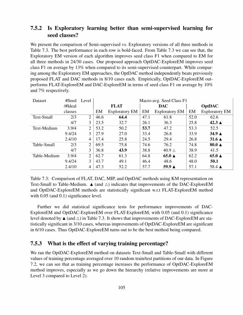
7.5.2 Is Exploratory learning better than semi-supervised learning forseed classes?

We present the comparison of Semi-supervised vs. Exploratory versions of all three methods inTable 7.3. The best performance in each row is bold-faced. From Table 7.3 we can see that, theExploratory EM version of each algorithm improves seed class F1 when compared to EM forall three methods in 24/30 cases. Our proposed approach OptDAC-ExploreEM improves seedclass F1 on average by 13% when compared to its semi-supervised counterpart. While compar-ing among the Exploratory EM approaches, the OptDAC method independently beats previouslyproposed FLAT and DAC methods in 8/10 cases each. Empirically, OptDAC-ExploreEM out-performs FLAT-ExploreEM and DAC-ExploreEM in terms of seed class F1 on average by 10%and 7% respectively.

Dataset #Seed Level Macro-avg. Seed Class F1/#Ideal FLAT DAC OptDACclasses EM Exploratory EM EM Exploratory EM EM Exploratory EM

Text-Small 2/3 2 46.6 64.4 47.1 61.8 52.0 62.64/7 3 23.5 32.7 26.1 36.3 25.8 42.3 N

Text-Medium 3.9/4 2 53.2 50.2 53.7 47.2 53.3 52.59.4/24 3 27.9 27.0 33.4 26.8 33.9 34.9 N2.4/10 4 17.4 25.8 24.5 29.4 26.8 31.6 N

Table-Small 2/3 2 69.5 75.8 74.6 76.2 74.8 80.0 N4/7 3 36.8 43.9 38.8 40.9 M 38.9 41.5

Table-Medium 3.9/4 2 62.7 61.3 64.8 65.0 N 62.2 65.0 N9.4/24 3 43.7 49.1 46.4 48.6 48.0 50.12.4/10 4 47.3 52.2 57.7 59.9 N 57.1 58.4 N

Table 7.3: Comparison of FLAT, DAC, MIP, and OptDAC methods using KM representation onText-Small to Table-Medium. N (and M) indicates that improvements of the DAC-ExploreEMand OptDAC-ExploreEM methods are statistically significant w.r.t FLAT-ExploreEM methodwith 0.05 (and 0.1) significance level.

Further we did statistical significance tests for performance improvements of DAC-ExploreEM and OptDAC-ExploreEM over FLAT-ExploreEM, with 0.05 (and 0.1) significancelevel denoted by N (and M) in Table 7.3. It shows that improvements of DAC-ExploreEM are sta-tistically significant in 3/10 cases, whereas improvements of OptDAC-ExploreEM are significantin 6/10 cases. Thus OptDAC-ExploreEM turns out to be the best method being compared.

7.5.3 What is the effect of varying training percentage?We ran the OptDAC-ExploreEM method on datasets Text-Small and Table-Small with differentvalues of training percentage averaged over 10 random train/test partitions of our data. In Figure7.2, we can see that as training percentage increases the performance of OptDAC-ExploreEMmethod improves, especially as we go down the hierarchy (relative improvements are more atLevel 3 compared to Level 2).

105

0 50 10020

30

40

50

60

70

80

Training percentage

Ma

cro

av

g.

se

ed

cla

ss

F1

0 50 10020

40

60

80

100

Training percentage

Ma

cro

av

g.

se

ed

cla

ss

F1

Level 2

Level 3

Figure 7.2: Comparison of OptDAC-ExploreEM method with different training percentage ondatasets Text-Small (left) and Table-Small (right).

7.5.4 How do the methods compare in terms of runtime?Here we compare runtimes of all methods averaged over all the runs with different seed ontolo-gies and seed training data. In our MATLAB implementation, the running time of ExploratoryEM is much longer. Table ?? shows that the increase in runtime of Exploratory EM variants w.r.t.their EM counterparts is by the factor 3.2 on average across all methods and datasets. Furtherthe exploratory methods take on average 10.3 times when compared to EM variant of the FLATmethod.

In particular, OptDAC-ExploreEM method is on average twice as expensive as DAC-ExploreEM. This is due to the fact that DAC-ExploreEM takes greedy decisions at each levelof the hierarchy, whereas OptDAC-ExploreEM keeps track of the top-q active nodes. We setq = 2 in these experiments. Thus the value of q results in a trade-off between improvement inseed class F1 and increased runtime of the algorithm.

7.5.5 Evaluation of extended cluster hierarchiesIn this section, we present the evaluation of extra clusters added by our Hierarchical ExploratoryEM algorithm to the incomplete class ontology given as input. If it started with k classes, andproduced k+m classes as output, we first need to label these m extra classes. Since our datasetsare completely labeled, each new class can be assigned a majority label based on entities assignedto that class and level of the class in the hierarchy. For Example, if the class is at level 2 in thehierarchy then we choose the best label at level 2 of the class hierarchy.

Figure 7.3 shows an example of an extended class hierarchy generated by OptDAC-ExploreEM algorithm on Table-Small starting with 7 seed classes from onto-1. The bold-facednodes are from the seed ontology, and nodes in blue (non bold-faced) are the ones added by ourproposed exploratory learning methods. It is labeled using the above described majority labelapproach. (Note that there are multiple clusters with same label, to differentiate them we havelabeled them as “Food 1”, “Food 2” etc.)

Once this labeling is done, we can measure the precision of labels across (parent, child)links in the cluster hierarchy. For Example, in Figure 7.3, parent-child link between (Food 2,

106

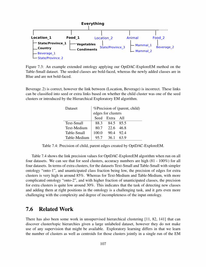
Figure 7.3: An example extended ontology applying our OptDAC-ExploreEM method on theTable-Small dataset. The seeded classes are bold-faced, whereas the newly added classes are inBlue and are not bold-faced.

Beverage 2) is correct, however the link between (Location, Beverage) is incorrect. These linkscan be classified into seed or extra links based on whether the child cluster was one of the seedclusters or introduced by the Hierarchical Exploratory EM algorithm.

Dataset %Precision of (parent, child)edges for clustersSeed Extra All

Text-Small 88.3 84.5 85.5Text-Medium 80.7 22.6 46.8Table-Small 100.0 90.4 92.4Table-Medium 95.7 36.1 63.9

Table 7.4: Precision of child, parent edges created by OptDAC-ExploreEM.

Table 7.4 shows the link precision values for OptDAC-ExploreEM algorithm when run on allfour datasets. We can see that for seed clusters, accuracy numbers are high (81 - 100%) for allfour datasets. In terms of extra clusters, for the datasets Text-Small and Table-Small with simplerontology “onto-1”, and unanticipated class fraction being low, the precision of edges for extraclusters is very high in around 85%. Whereas for Text-Medium and Table-Medium, with morecomplicated ontology “onto-2”, and with higher fraction of unanticipated classes, the precisionfor extra clusters is quite low around 30%. This indicates that the task of detecting new classesand adding them at right positions in the ontology is a challenging task, and it gets even morechallenging with the complexity and degree of incompleteness of the input ontology.

7.6 Related WorkThere has also been some work in unsupervised hierarchical clustering [11, 82, 141] that candiscover cluster/topic hierarchies given a large unlabeled dataset, however they do not makeuse of any supervision that might be available. Exploratory learning differs in that we learnthe number of clusters as well as centroids for those clusters jointly in a single run of the EM

107

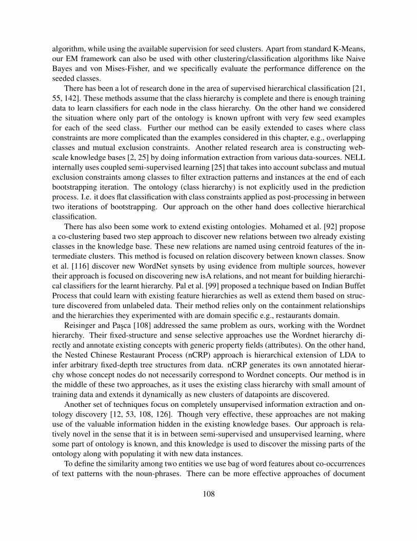
algorithm, while using the available supervision for seed clusters. Apart from standard K-Means,our EM framework can also be used with other clustering/classification algorithms like NaiveBayes and von Mises-Fisher, and we specifically evaluate the performance difference on theseeded classes.

There has been a lot of research done in the area of supervised hierarchical classification [21,55, 142]. These methods assume that the class hierarchy is complete and there is enough trainingdata to learn classifiers for each node in the class hierarchy. On the other hand we consideredthe situation where only part of the ontology is known upfront with very few seed examplesfor each of the seed class. Further our method can be easily extended to cases where classconstraints are more complicated than the examples considered in this chapter, e.g., overlappingclasses and mutual exclusion constraints. Another related research area is constructing web-scale knowledge bases [2, 25] by doing information extraction from various data-sources. NELLinternally uses coupled semi-supervised learning [25] that takes into account subclass and mutualexclusion constraints among classes to filter extraction patterns and instances at the end of eachbootstrapping iteration. The ontology (class hierarchy) is not explicitly used in the predictionprocess. I.e. it does flat classification with class constraints applied as post-processing in betweentwo iterations of bootstrapping. Our approach on the other hand does collective hierarchicalclassification.

There has also been some work to extend existing ontologies. Mohamed et al. [92] proposea co-clustering based two step approach to discover new relations between two already existingclasses in the knowledge base. These new relations are named using centroid features of the in-termediate clusters. This method is focused on relation discovery between known classes. Snowet al. [116] discover new WordNet synsets by using evidence from multiple sources, howevertheir approach is focused on discovering new isA relations, and not meant for building hierarchi-cal classifiers for the learnt hierarchy. Pal et al. [99] proposed a technique based on Indian BuffetProcess that could learn with existing feature hierarchies as well as extend them based on struc-ture discovered from unlabeled data. Their method relies only on the containment relationshipsand the hierarchies they experimented with are domain specific e.g., restaurants domain.

Reisinger and Pasca [108] addressed the same problem as ours, working with the Wordnethierarchy. Their fixed-structure and sense selective approaches use the Wordnet hierarchy di-rectly and annotate existing concepts with generic property fields (attributes). On the other hand,the Nested Chinese Restaurant Process (nCRP) approach is hierarchical extension of LDA toinfer arbitrary fixed-depth tree structures from data. nCRP generates its own annotated hierar-chy whose concept nodes do not necessarily correspond to Wordnet concepts. Our method is inthe middle of these two approaches, as it uses the existing class hierarchy with small amount oftraining data and extends it dynamically as new clusters of datapoints are discovered.

Another set of techniques focus on completely unsupervised information extraction and on-tology discovery [12, 53, 108, 126]. Though very effective, these approaches are not makinguse of the valuable information hidden in the existing knowledge bases. Our approach is rela-tively novel in the sense that it is in between semi-supervised and unsupervised learning, wheresome part of ontology is known, and this knowledge is used to discover the missing parts of theontology along with populating it with new data instances.

To define the similarity among two entities we use bag of word features about co-occurrencesof text patterns with the noun-phrases. There can be more effective approaches of document

108

representation like the lower dimensional continuous Skip-gram features, proposed by Mikolovet al. [89]. Their technique learns low dimensional vectors that potentially embed semantics ofnoun-phrases.

7.7 ConclusionsWe propose the Hierarchical Exploratory EM approach that can take an incomplete seed ontologyas input, along with a few examples of each seed class, to populate new instances of seed classesand extend the ontology with newly discovered classes. Experiments with subsets of the NELLontology and and text, semi-structured HTML table datasets derived from the ClueWeb09 corpusshow encouraging results in terms of seed class F1 scores.

Our proposed hierarchical exploratory EM method, named OptDAC-ExploreEM performsbetter than flat classification and hierarchical semi-supervised EM methods at all levels of hierar-chy, especially as we go further down the hierarchy. Experiments show that OptDAC-ExploreEMoutperforms its semi-supervised variant on average by 13% in terms of seed class F1 scores. Italso outperforms both previously proposed exploratory learning approaches FLAT-ExploreEMand DAC-ExploreEM in terms of seed class F1 on average by 10% and 7% respectively.

7.8 Future Research DirectionsIn the future, we would like to apply our method on datasets with larger and non-tree structuredclass hierarchies. We briefly discussed how our proposed OptDAC-ExploreEM method can beused for this task. Further, our experiments focused on an information extraction task of classi-fying entities into a knowledge base class hierarchy. However, our techniques can also be usedfor other tasks like document classification into topic hierarchies on datasets like Reuters, andclassifying images into a class hierarchy for datasets like ImageNet.

109

110

Chapter 8

Concluding Remarks

Here, we first summarize the overall contributions, then we list the observations from experi-ments presented in different chapters of this thesis. Finally, we also present the potential futuredirections for this research.

8.1 Thesis SummaryWe proposed several extensions to the traditional semi-supervised learning algorithm using Ex-pectation Maximization. Combining all these extensions leads to a generic semi-supervisedlearning framework that can incorporate 1) the presence of unanticipated classes, 2) multipledata views, and 3) ontological class constraints. This framework helps reduce semantic drift onknown seeded classes as well as provides a single method that solves a continuum of tasks fromsupervised learning to clustering. In both flat and hierarchical classification/clustering settings,we observed that running an algorithm in an exploratory setting gave comparable or better seedclass F1 score when compared to the traditional semi-supervised counterpart [124, 127, 128].

Further, exploratory learning is more powerful in conjunction with ontological class con-straints which can be imposed as soft constraints on the label vectors assigned to a datapoint. Wealso found that considering ontological constraints while inferring labels improves overall per-formance compared to flat classification for the the entity classification and gloss finding tasks[124, 127, 130]. Through experiments in this thesis, we showed that a single semi-supervisedlearning framework could handle NLP tasks like entity/document classification, entity/wordsense disambiguation, gloss finding and ontology extension. Code for the flat exploratory K-Means, GLOFIN algorithm and most of the datasets we created during this research can be down-loaded from http://rtw.ml.cmu.edu/wk/WebSets/exploratory_learning/.

Contributions

In this thesis we first proposed exploratory learning techniques (Chapter 4) that improve therobustness of semi-supervised learning methods to the presence of unanticipated classes in theunlabeled data, thereby reducing semantic drift of seeded classes. Exploratory EM introducesnew classes on-the-fly during learning based on the intuition that hard-to-classify examples—specifically, examples with a nearly-uniform posterior class distribution—should be assigned to

111

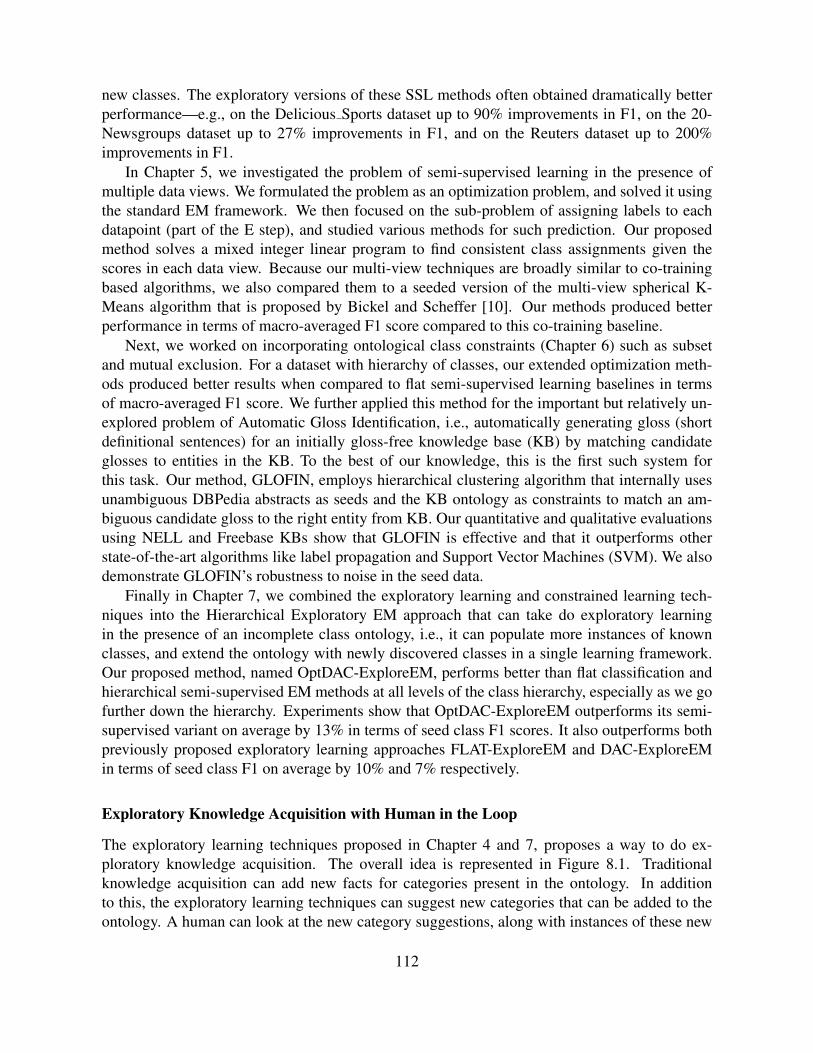
new classes. The exploratory versions of these SSL methods often obtained dramatically betterperformance—e.g., on the Delicious Sports dataset up to 90% improvements in F1, on the 20-Newsgroups dataset up to 27% improvements in F1, and on the Reuters dataset up to 200%improvements in F1.

In Chapter 5, we investigated the problem of semi-supervised learning in the presence ofmultiple data views. We formulated the problem as an optimization problem, and solved it usingthe standard EM framework. We then focused on the sub-problem of assigning labels to eachdatapoint (part of the E step), and studied various methods for such prediction. Our proposedmethod solves a mixed integer linear program to find consistent class assignments given thescores in each data view. Because our multi-view techniques are broadly similar to co-trainingbased algorithms, we also compared them to a seeded version of the multi-view spherical K-Means algorithm that is proposed by Bickel and Scheffer [10]. Our methods produced betterperformance in terms of macro-averaged F1 score compared to this co-training baseline.

Next, we worked on incorporating ontological class constraints (Chapter 6) such as subsetand mutual exclusion. For a dataset with hierarchy of classes, our extended optimization meth-ods produced better results when compared to flat semi-supervised learning baselines in termsof macro-averaged F1 score. We further applied this method for the important but relatively un-explored problem of Automatic Gloss Identification, i.e., automatically generating gloss (shortdefinitional sentences) for an initially gloss-free knowledge base (KB) by matching candidateglosses to entities in the KB. To the best of our knowledge, this is the first such system forthis task. Our method, GLOFIN, employs hierarchical clustering algorithm that internally usesunambiguous DBPedia abstracts as seeds and the KB ontology as constraints to match an am-biguous candidate gloss to the right entity from KB. Our quantitative and qualitative evaluationsusing NELL and Freebase KBs show that GLOFIN is effective and that it outperforms otherstate-of-the-art algorithms like label propagation and Support Vector Machines (SVM). We alsodemonstrate GLOFIN’s robustness to noise in the seed data.

Finally in Chapter 7, we combined the exploratory learning and constrained learning tech-niques into the Hierarchical Exploratory EM approach that can take do exploratory learningin the presence of an incomplete class ontology, i.e., it can populate more instances of knownclasses, and extend the ontology with newly discovered classes in a single learning framework.Our proposed method, named OptDAC-ExploreEM, performs better than flat classification andhierarchical semi-supervised EM methods at all levels of the class hierarchy, especially as we gofurther down the hierarchy. Experiments show that OptDAC-ExploreEM outperforms its semi-supervised variant on average by 13% in terms of seed class F1 scores. It also outperforms bothpreviously proposed exploratory learning approaches FLAT-ExploreEM and DAC-ExploreEMin terms of seed class F1 on average by 10% and 7% respectively.

Exploratory Knowledge Acquisition with Human in the Loop

The exploratory learning techniques proposed in Chapter 4 and 7, proposes a way to do ex-ploratory knowledge acquisition. The overall idea is represented in Figure 8.1. Traditionalknowledge acquisition can add new facts for categories present in the ontology. In additionto this, the exploratory learning techniques can suggest new categories that can be added to theontology. A human can look at the new category suggestions, along with instances of these new

112

categories, to pick the ones that look meaningful.This kind of learning mechanism is in between open domain knowledge extraction and closed

domain (ontology driven) knowledge extraction, i.e., it can make use of the available training dataand at the same time discover new categories from unlabeled data.

Figure 8.1: Exploratory Knowledge Acquisition with Human in the Loop.

8.2 Future Research DirectionsThis thesis opens up many interesting directions for future research. A most straightforwardfuture work can be to understand how well our exploratory learning techniques work for datasetswhere the classes are not clearly separable (overlapping topics). It would also be interesting toanalyze what fraction of classes need to be seeded to be able to discover the rest of them fromunlabeled data.

The intuitions behind our techniques can be used to extend few other techniques to makethem more effective. Further, the techniques proposed in this thesis are not limited to the taskspresented in this thesis. Next, we explain some of these future directions in terms of advance-ments in terms of the techniques and applications.

New Techniques:

Naming the Newly Discovered Concepts

Apart from reducing the semantic drift of seeded classes, another important advantage of ex-ploratory learning methods is to discover multiple clusters of datapoints that did not fit any of theclasses given to the algorithm. These are potentially new concepts that can be added to an exist-ing knowledge base. For example, in our experiments with the WebSets table corpus and NELLKB, we found that with some manual inspection, our system could add good quality conceptslike “music scales”, “dental procedures” etc., that were missing in the NELL KB.

113

Automatically naming the newly discovered clusters of entities is another interesting direc-tion of future research. In Chapter 3, we described one such technique, i.e. those hypernymsthat occurred with the candidate entities in the context of Hearst patterns were used as candidatelabels for newly discovered clusters. Another way to achieve this could be to describe a clusterby the centroid for the cluster. For Example, for a newly discovered cluster of news stories, witha bag of words feature representation and TFIDF weights, a centroid feature vector will give usthe top distinguishing words that occurred most frequently in the cluster.

Exploratory Extensions of Mixed-Membership Methods

Our proposed Exploratory Learning technique [128] shows that the near uniformity heuristicif applied to Chinese Restaurant Process, gives performance gains in terms of seed class F1 andrunning times (Chapter 4). Exploratory EM in its current form is a hard-EM algorithm, i.e., in theE step each datapoint gets assigned to only one of the clusters/classes. It would be an interestingdirection of future research to build mixed-membership exploratory learning techniques, i.e., asoft-EM version of our algorithm, and use modified CRP process, to induce new clusters.

New Applications:Word Sense Disambiguation using WordNet Hierarchy

We are currently working on using our hierarchical semi-supervised learning technique, GLOFIN(refer Chapter 6), for the task of word sense disambiguation with respect to WordNet. Here weconsider occurrences of all unambiguous words as training data and ambiguous word occur-rences as unlabeled data. In these experiments, we use the WordNet synset hierarchy to deduceontological constraints. Figure 8.2 shows an example of synset hierarchy around word ‘goal’.Further we plan to use clues from two different data views: glosses and example usages of theword senses.

Exploratory Relation Extraction

Most techniques discussed in this thesis are not tied to any particular document representation,choice of features or task. Hence one obvious future research direction lies in applying theseideas to tasks other than concept extraction. For example, Relation extraction is a very challeng-ing task, and many ontologies like NELL that are rich in terms of coverage of concepts have lowcoverage in terms of relations between entities. We hope that the Exploratory learning techniquecan be extended for the relation extraction task.

114

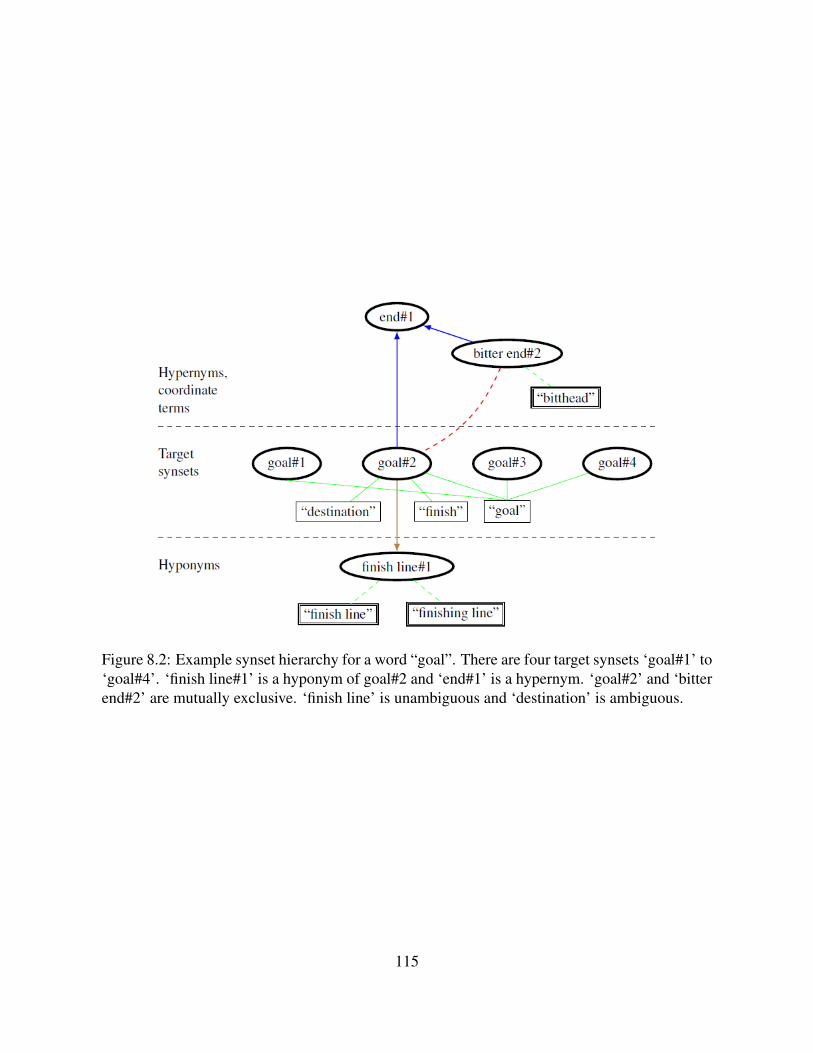
Figure 8.2: Example synset hierarchy for a word “goal”. There are four target synsets ‘goal#1’ to‘goal#4’. ‘finish line#1’ is a hyponym of goal#2 and ‘end#1’ is a hypernym. ‘goal#2’ and ‘bitterend#2’ are mutually exclusive. ‘finish line’ is unambiguous and ‘destination’ is ambiguous.

115

116

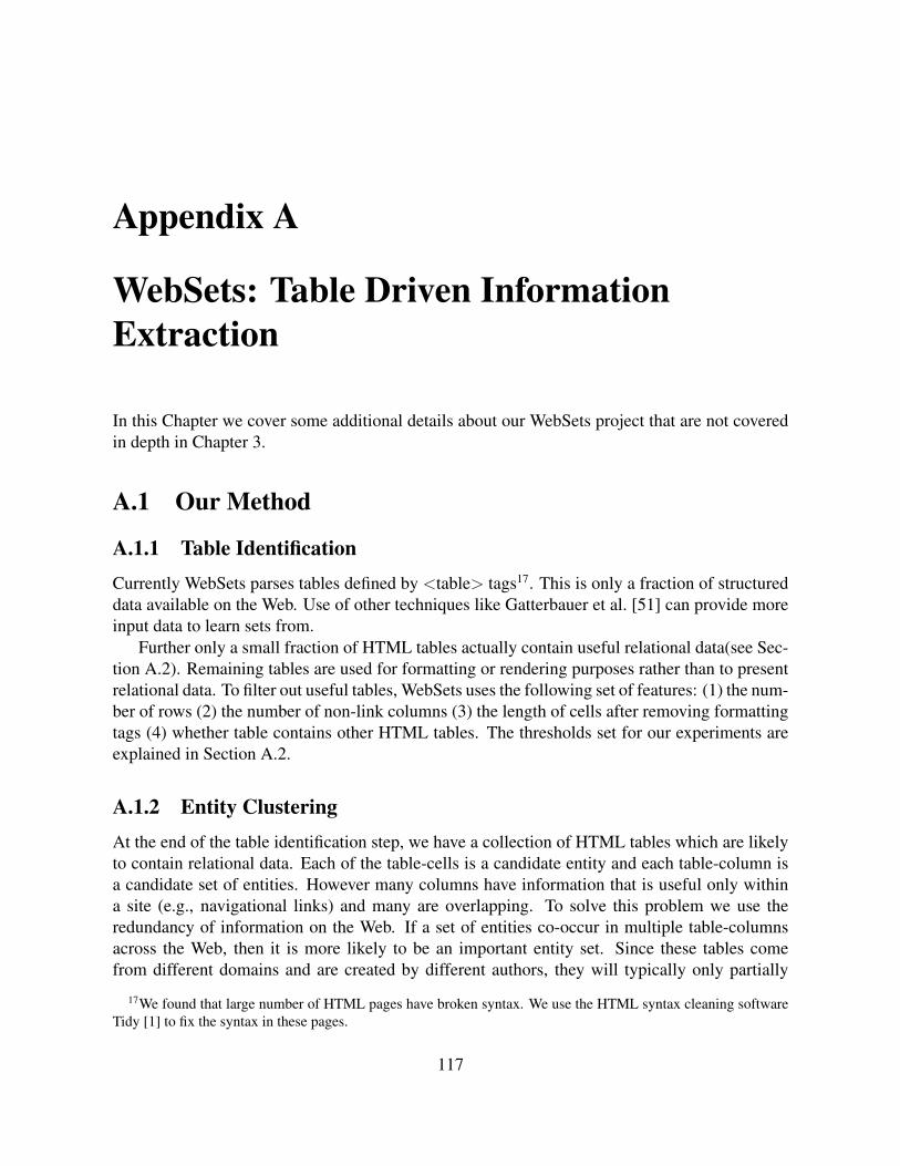
Appendix A

WebSets: Table Driven InformationExtraction

In this Chapter we cover some additional details about our WebSets project that are not coveredin depth in Chapter 3.

A.1 Our Method

A.1.1 Table IdentificationCurrently WebSets parses tables defined by <table> tags17. This is only a fraction of structureddata available on the Web. Use of other techniques like Gatterbauer et al. [51] can provide moreinput data to learn sets from.

Further only a small fraction of HTML tables actually contain useful relational data(see Sec-tion A.2). Remaining tables are used for formatting or rendering purposes rather than to presentrelational data. To filter out useful tables, WebSets uses the following set of features: (1) the num-ber of rows (2) the number of non-link columns (3) the length of cells after removing formattingtags (4) whether table contains other HTML tables. The thresholds set for our experiments areexplained in Section A.2.

A.1.2 Entity ClusteringAt the end of the table identification step, we have a collection of HTML tables which are likelyto contain relational data. Each of the table-cells is a candidate entity and each table-column isa candidate set of entities. However many columns have information that is useful only withina site (e.g., navigational links) and many are overlapping. To solve this problem we use theredundancy of information on the Web. If a set of entities co-occur in multiple table-columnsacross the Web, then it is more likely to be an important entity set. Since these tables comefrom different domains and are created by different authors, they will typically only partially

17We found that large number of HTML pages have broken syntax. We use the HTML syntax cleaning softwareTidy [1] to fix the syntax in these pages.

117

Country Capital CityIndia DelhiChina BeijingCanada OttawaFrance Paris

Table A.1: TableId= 21, domain= “www.dom1.com”

overlap. To cluster the entities in these columns into coherent sets, the first essential step willbe to represent this data in a way that reveals the co-occurrence of entities across multiple tablecolumns. In this section, we will first discuss the data representation, and then algorithms forentity clustering.

Data Representation

We considered two ways to represent table data. With the “Entity record representation”, onerecord per entity is created, and it contains information about which table-columns and URLdomains the entity was mentioned in. These entity records can then be clustered, based on theoverlap of table-columns and domains, to yield sets of entities. One advantage of this represen-tation is that it is compact. Another advantage is that the number of distinct domains an entityoccurred in can be used as an indicator of how “important” it is. A disadvantage of this represen-tation is that if some entity-name is ambiguous (has multiple senses), it will collapse all sensesof the entity into one record. For example, consider a corpus which contains mentions of theentity “Apple” in two senses, “Apple as a fruit” and “Apple as a company”. This representationwill create a single record for the entity “Apple” with its occurrence as a fruit and as a companyconfounded. An unsupervised IE system might find it difficult to decompose multiple sensesfrom this single record.

To solve this problem, we propose a novel representation of the table data called “Entity-Triplet records”. In this representation, there is a record for each triplet of adjacent entitiesinstead of for individual entities. Each record contains information about which table-columnsand URL domains the triplet occurred in. Hence in case of an ambiguous entity like “Apple”, itsoccurrences as a fruit will be separate from its occurrences as a company, e.g., Apple, Avocado,Banana will be one triplet record and Apple, Microsoft, DELL will be another triplet record.Thus entities within a triplet disambiguate each other. Since we have a list of all domains a tripletoccurred in, only those triplets which appear in enough domains can be considered as important.

In this way, we represent the table data as a triplet store, which contains a record for eachentity triplet. The triplet store can be built in one single pass over the corpus. If the systemconsiders all possible triplets that can be created from each table column, then number of tripletrecords will be quadratic in the total size of all tables. This can be a serious concern for aweb-scale dataset. Hence our system constructs only those triplets which are adjacent i.e. sub-sequences of entities in a table-column. This ensures that number of triplet records are linear intotal size of all tables, making the system scalable. The system keeps track of all table-columnsa triplet occurred in, which makes it possible to reconstruct a column by joining triplets oncolumnId. Hence this storage method does not result in any loss of information.

Consider an example of tables containing countries and their capitals. Original tables are

118

Country Capital CityChina BeijingCanada OttawaFrance ParisEngland London

Table A.2: TableId= 34, URL= “www.dom2.com”

Entities Tid:Cids DomainsIndia,China,Canada 21:1 www.dom1.comChina, Canada, France 21:1, 34:1 www.dom1.com, www.dom2.comDelhi, Beijing, Ottawa 21:2 www.dom1.comBeijing, Ottawa, Paris 21:2, 34:2 www.dom1.com, www.dom2.comCanada, England, France 34:1 www.dom2.comLondon, Ottawa, Paris 34:2 www.dom2.com

Table A.3: Triplet records created by WebSets

shown in Table A.1, A.2 and the triplet records created by WebSets are shown in Table A.3.Second row in Table A.3, indicates that the triplet (China, Canada, France) occurred in column 1of tableId 21 and column 1 of tableId 34. Also these entities are retrieved from webpages whichreside in the domains “www.dom1.com” and “www.dom2.com”.

These triplets are canonicalized by converting entity strings to lower case and arranging theconstituent entities in alphabetical order. The triplets are then ranked in descending order ofnumber of domains.

We createO(n) triplets from a table column of size n. Adding each triplet to the Triplet Storeusing hashmap takesO(1) time. Given a set of T HTML tables with a total ofN entities in them,the Triplet Store can be created in O(N) time. Ranking the triplets using any common sortingtechnique will take O(N ∗ logN) time. Hence the total complexity of building the Triplet Storeis O(N ∗ logN).

Building entity clusters

The next task is to cluster these triplet records into meaningful sets. The system does not knowhow many clusters are present in the underlying dataset; and since our dataset will be constructedfrom a huge HTML web corpus, the clustering algorithm needs to be very efficient. Given theserequirements, it can be easily seen that parametric clustering algorithms like K-means may not beeffective due to the unknown number of clusters. Non-parametric algorithms like agglomerativeclustering [35] fit most of our requirements. The most efficient agglomerative clustering algo-rithm is the single-link clustering algorithm, but even that would require computing the similarityof every pair of entity triplets returned. This will be very expensive for the web scale datasets weare aiming to handle. Hence we develop a new bottom-up clustering algorithm which is efficientin terms of both space and time. Experiments to compare our algorithm with a standard K-meansclustering algorithm are described in Section A.2.

119

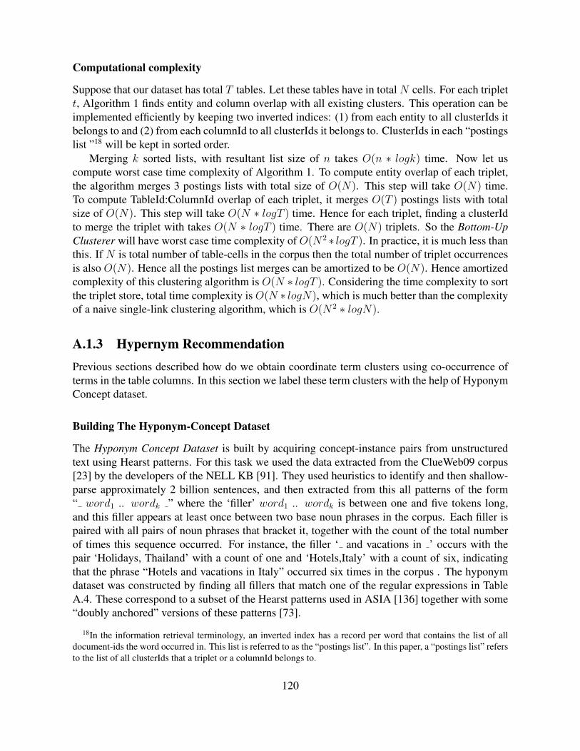
Computational complexity

Suppose that our dataset has total T tables. Let these tables have in total N cells. For each triplett, Algorithm 1 finds entity and column overlap with all existing clusters. This operation can beimplemented efficiently by keeping two inverted indices: (1) from each entity to all clusterIds itbelongs to and (2) from each columnId to all clusterIds it belongs to. ClusterIds in each “postingslist ”18 will be kept in sorted order.

Merging k sorted lists, with resultant list size of n takes O(n ∗ logk) time. Now let uscompute worst case time complexity of Algorithm 1. To compute entity overlap of each triplet,the algorithm merges 3 postings lists with total size of O(N). This step will take O(N) time.To compute TableId:ColumnId overlap of each triplet, it merges O(T ) postings lists with totalsize of O(N). This step will take O(N ∗ logT ) time. Hence for each triplet, finding a clusterIdto merge the triplet with takes O(N ∗ logT ) time. There are O(N) triplets. So the Bottom-UpClusterer will have worst case time complexity of O(N2 ∗ logT ). In practice, it is much less thanthis. If N is total number of table-cells in the corpus then the total number of triplet occurrencesis also O(N). Hence all the postings list merges can be amortized to be O(N). Hence amortizedcomplexity of this clustering algorithm is O(N ∗ logT ). Considering the time complexity to sortthe triplet store, total time complexity is O(N ∗ logN), which is much better than the complexityof a naive single-link clustering algorithm, which is O(N2 ∗ logN).

A.1.3 Hypernym RecommendationPrevious sections described how do we obtain coordinate term clusters using co-occurrence ofterms in the table columns. In this section we label these term clusters with the help of HyponymConcept dataset.

Building The Hyponym-Concept Dataset

The Hyponym Concept Dataset is built by acquiring concept-instance pairs from unstructuredtext using Hearst patterns. For this task we used the data extracted from the ClueWeb09 corpus[23] by the developers of the NELL KB [91]. They used heuristics to identify and then shallow-parse approximately 2 billion sentences, and then extracted from this all patterns of the form“ word1 .. wordk ” where the ‘filler’ word1 .. wordk is between one and five tokens long,and this filler appears at least once between two base noun phrases in the corpus. Each filler ispaired with all pairs of noun phrases that bracket it, together with the count of the total numberof times this sequence occurred. For instance, the filler ‘ and vacations in ’ occurs with thepair ‘Holidays, Thailand’ with a count of one and ‘Hotels,Italy’ with a count of six, indicatingthat the phrase “Hotels and vacations in Italy” occurred six times in the corpus . The hyponymdataset was constructed by finding all fillers that match one of the regular expressions in TableA.4. These correspond to a subset of the Hearst patterns used in ASIA [136] together with some“doubly anchored” versions of these patterns [73].

18In the information retrieval terminology, an inverted index has a record per word that contains the list of alldocument-ids the word occurred in. This list is referred to as the “postings list”. In this paper, a “postings list” refersto the list of all clusterIds that a triplet or a columnId belongs to.

120

Id Regular expression1 arg1 such as (w+ (and|or))? arg22 arg1 (w+ )? (and|or) other arg23 arg1 include (w+ (and|or))? arg24 arg1 including (w+ (and|or))? arg2

Table A.4: Regular expressions used to create Hyponym Concept Dataset

Hyponym ConceptsUSA country:1000India country:200Paris city:100, tourist place:50

Monkey animal:100, mammal:60Sparrow bird:33

Table A.5: An example of Hyponym Concept Dataset

Each record in the Hyponym Concept Dataset contains an entity and all concepts it co-occurred with. Table A.5 shows an example of records in this dataset. According to this table,entity “USA” appeared with the concept “country” 1000 times. Similarly, “Monkey” appearedwith two different concepts, 100 times with “animal” and 60 times with “mammal”.

Assigning Hypernyms to Clusters

Assigning a meaningful concept-name to each entity set is important for two reasons. It enablesus to systematically evaluate entity sets; e.g., it is easier for an evaluator to answer the question:“Is Boston a city?” than “Is Boston a member of set #37?”) It also makes the system more usefulfor summarizing the data in a corpus (see Section 3.1.3). This section describes how WebSetsrecommends candidate hypernyms for each entity set produced by Algorithm 1.

For this task, we use the coordinate term clusters extracted from tables and Hyponym Con-cept Dataset extracted using Hearst patterns. Note that this part of the system uses informationextracted from unstructured text from the Web, to recommend category names to sets extractedfrom tables on the Web.

A.2 Evaluation of Individual Stages of WebSetsIn this section we evaluate each stage of WebSets system and measure the performance. Herewe consider WebSets as a technique to generate large number of concept-instance pairs given aHTML corpus.

A.2.1 Evaluation: Table IdentificationTable A.6 shows the statistics of table identification for each dataset. Based on the featuresdescribed in Section A.1.1, we filter out only those tables as useful which cross some predefinedthresholds. These thresholds were derived from the intuitions after manually going through somesamples of data, and are kept constant for all datasets and experiments described in this paper.

121

Dataset #Tables %Rela- #Filtered %Rela- #Triplets-tional tables -tional

filteredToy Apple 2.6K 50 762 75 15KDelicious Sports 146.3K 15 57.0K 55 63KDelicious Music 643.3K 20 201.8K 75 93KCSEAL Useful 322.8K 30 116.2K 80 1148KASIA NELL 676.9K 20 233.0K 55 421KASIA INT 621.3K 15 216.0K 60 374KClueweb HPR 586.9K 10 176.0K 35 78K

Table A.6: Table Identification Statistics

When we evaluated a random sample of recursive tables, 93% of them were useless for ourpurposes, and only 7% tables contained relational data. Hence we decide to ignore the recursivetables. We construct triplets of entities in a table column, hence a table should have at least 3rows. As we are not using any link data in our system, we consider only those columns whichdo not have links. WebSets is looking for tables containing relational data, hence if a table has atleast 2 non-link columns, probability of it having relational data increases. While counting theserows and columns, we are looking for named entities. So from each cell, all HTML tags andlinks are removed. A very coarse filtering by length is then applied. We consider only those tablecells which are 2-50 characters in length. Table A.6 shows that percentage of relational tablesincreases by orders of magnitude due to this filtering step.

A.2.2 Evaluation: Clustering Algorithm

In these set of experiments we first compare WebSets with baseline K-means clustering algo-rithm. Later we see how “Entity-Triplet record” representation is better than “Entity record”representation. We compare the clustering algorithms in terms of commonly used clusteringmetrics: cluster purity (Purity), normalized mutual information (NMI), rand index (RI) [82] andFowlkes-Mallows index (FM) which are defined as follows:• Cluster Purity: To compute cluster purity, for each cluster the class which is most frequent

in it gets assigned. The accuracy of this assignment is then measured by counting thenumber of correctly assigned documents and dividing by total number of documents.purity(Ω, C) = 1

N

∑k maxj |ωk

⋂cj| where

N is total number of documents, Ω = ω1, ω2, ..., ωKis the set of clusters and C = c1, c2, ..., cJ is the set of classes. We interpret ωk as the setof documents in cluster ωk and cj as the set of documents in cluster cj .

• Normalized Mutual Information: High purity is easy to achieve when the number ofclusters is large, hence purity cannot be used to trade off the quality of the clusteringagainst the number of clusters. NMI is a measure that allows us to make such tradeoff.NMI(Ω, C) = I(Ω;C)

[H(Ω)+H(C)]/2

where maximum likelihood estimates for mutual information and entropy are computed asfollows:I(Ω, C) =

∑k

∑j|ωk

⋂cj |

N, H(Ω) = −

∑k|ωk|N∗ log |ωk|

N.

122

• Rand Index: This metric is based on information-theoretic interpretation of clustering.Clustering is a series of decisions, one for each of the N(N − 1)/2 pairs of documents inthe collection. True label denotes the pair belongs to same class or not. Predicted labeldenotes whether the pair belongs to same cluster or not. This way we can count TruePositive(TP ), False positive (FP ), True Negative (TN ) and False Negative (FN ) scorefor the clustering. Rand Index is then defined as follows: RI = TP+TN

TP+FP+FN+TN.

• Fowlkes-Mallows index: While the previous three metrics are applicable only for hard-clustering, this metric is defined for soft clustering of data where clusters can be overlap-ping but classes are non-overlapping. Let nij be the size of intersection of cluster ωi andclass cj , ni∗ =

∑j nij and n∗j =

∑i nij .

FM = (∑

ij

(nij2

))/

√∑i

(ni∗2

)∑j

(n∗j2

)The derivation of this formula can be found in Ramirez et al. [106].

Here each triplet is considered as a document. Ω refers to clusters of these triplets generatedby WebSets or K-means. C refers to actual classes these triplets belong to. To compare qualityof clusters across algorithms, we manually labeled each table-column of Toy Apple and Deli-cious Sports datasets. These labels are then extended to triplets within the table column. Thisexperiment is not repeated for remaining datasets because manual labeling of the whole datasetis very expensive.

The performance of K-means depends on the input parameter K and random initialization ofcluster centroids to start the clustering process. We run K-means with cosine distance function,a range of values of K and multiple starting points for each value of K. Figure A.1 shows theplot of various runs of K-means vs. WebSets on Delicious Sports dataset. Table A.7 shows thecomparison of WebSets vs. best run of K-means on Toy Apple and Delicious Sports datasets.We can see that WebSets performs better or comparable to K-means in terms of purity, NMI, RI,and FM. Through manual labeling we found that there are 27 and 29 distinct category sets inToy Apple and Delicious Sports datasets respectively. We can see that WebSets defined 25 and32 distinct clusters which are very close to actual number of meaningful sets, compared to 40and 50 clusters defined by K-means.

Standard K-means algorithm has time complexity of O(I ∗ K ∗ N ∗ T ), where I is thenumber of iterations, K is the number of clusters, N is the number of table-cells and T is thenumber of dimensions (here number of table-columns). WebSets has time complexity of O(N ∗logN). Hence our bottom-up clustering algorithm is more efficient than K-means in terms oftime-complexity.

To study entity disambiguation effect of triplet records, we generated both “Entity record”and “Entity-Triplet record” representations of Toy Apple dataset. When we ran our clusteringalgorithm on “Entity-Triplet record” dataset, we found “Apple” in two different clusters, one inwhich it was clustered with other fruits and had supporting evidence from table-columns talk-ing about fruits; other cluster contained companies and evidence from related table-columns.Running the same clustering algorithm on “Entity record” dataset, resulted in a huge cluster con-taining “Apple”, fruits and companies all combined. Thus we can say that entity triplets do helpWebSets to disambiguate multiple senses of the same entity-string.

123

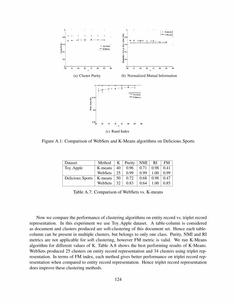
(a) Cluster Purity (b) Normalized Mutual Information

(c) Rand Index

Figure A.1: Comparison of WebSets and K-Means algorithms on Delicious Sports

Dataset Method K Purity NMI RI FMToy Apple K-means 40 0.96 0.71 0.98 0.41

WebSets 25 0.99 0.99 1.00 0.99Delicious Sports K-means 50 0.72 0.68 0.98 0.47

WebSets 32 0.83 0.64 1.00 0.85

Table A.7: Comparison of WebSets vs. K-means

Now we compare the performance of clustering algorithms on entity record vs. triplet recordrepresentation. In this experiment we use Toy Apple dataset. A table-column is consideredas document and clusters produced are soft-clustering of this document set. Hence each table-column can be present in multiple clusters, but belongs to only one class. Purity, NMI and RImetrics are not applicable for soft clustering, however FM metric is valid. We run K-Meansalgorithm for different values of K. Table A.8 shows the best performing results of K-Means.WebSets produced 25 clusters on entity record representation and 34 clusters using triplet rep-resentation. In terms of FM index, each method gives better performance on triplet record rep-resentation when compared to entity record representation. Hence triplet record representationdoes improve these clustering methods.

124

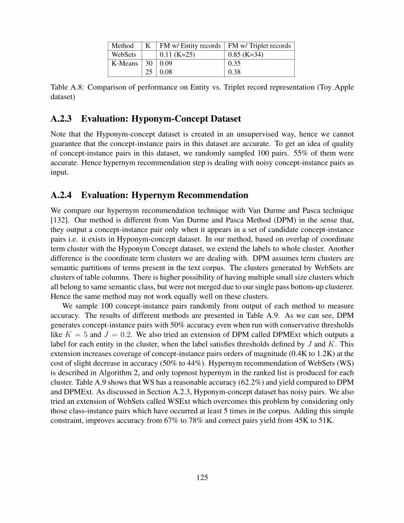
Method K FM w/ Entity records FM w/ Triplet recordsWebSets 0.11 (K=25) 0.85 (K=34)K-Means 30 0.09 0.35

25 0.08 0.38

Table A.8: Comparison of performance on Entity vs. Triplet record representation (Toy Appledataset)

A.2.3 Evaluation: Hyponym-Concept DatasetNote that the Hyponym-concept dataset is created in an unsupervised way, hence we cannotguarantee that the concept-instance pairs in this dataset are accurate. To get an idea of qualityof concept-instance pairs in this dataset, we randomly sampled 100 pairs. 55% of them wereaccurate. Hence hypernym recommendation step is dealing with noisy concept-instance pairs asinput.

A.2.4 Evaluation: Hypernym RecommendationWe compare our hypernym recommendation technique with Van Durme and Pasca technique[132]. Our method is different from Van Durme and Pasca Method (DPM) in the sense that,they output a concept-instance pair only when it appears in a set of candidate concept-instancepairs i.e. it exists in Hyponym-concept dataset. In our method, based on overlap of coordinateterm cluster with the Hyponym Concept dataset, we extend the labels to whole cluster. Anotherdifference is the coordinate term clusters we are dealing with. DPM assumes term clusters aresemantic partitions of terms present in the text corpus. The clusters generated by WebSets areclusters of table columns. There is higher possibility of having multiple small size clusters whichall belong to same semantic class, but were not merged due to our single pass bottom-up clusterer.Hence the same method may not work equally well on these clusters.

We sample 100 concept-instance pairs randomly from output of each method to measureaccuracy. The results of different methods are presented in Table A.9. As we can see, DPMgenerates concept-instance pairs with 50% accuracy even when run with conservative thresholdslike K = 5 and J = 0.2. We also tried an extension of DPM called DPMExt which outputs alabel for each entity in the cluster, when the label satisfies thresholds defined by J and K. Thisextension increases coverage of concept-instance pairs orders of magnitude (0.4K to 1.2K) at thecost of slight decrease in accuracy (50% to 44%). Hypernym recommendation of WebSets (WS)is described in Algorithm 2, and only topmost hypernym in the ranked list is produced for eachcluster. Table A.9 shows that WS has a reasonable accuracy (62.2%) and yield compared to DPMand DPMExt. As discussed in Section A.2.3, Hyponym-concept dataset has noisy pairs. We alsotried an extension of WebSets called WSExt which overcomes this problem by considering onlythose class-instance pairs which have occurred at least 5 times in the corpus. Adding this simpleconstraint, improves accuracy from 67% to 78% and correct pairs yield from 45K to 51K.

125

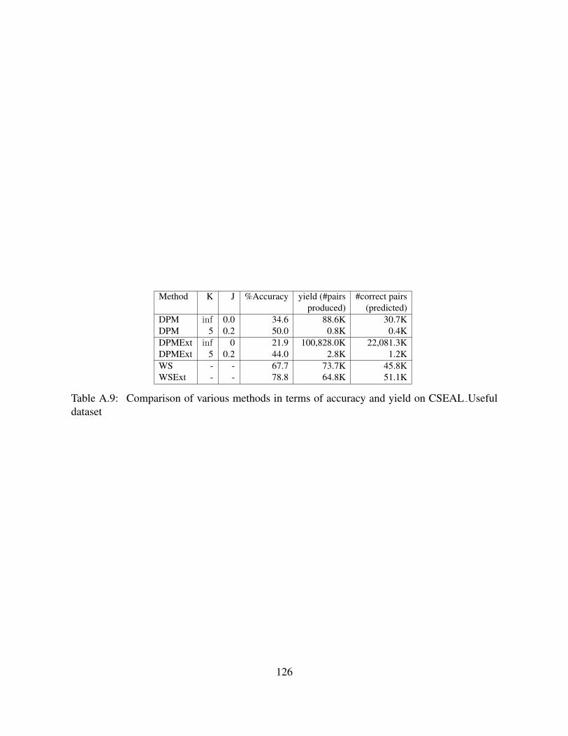
Method K J %Accuracy yield (#pairs #correct pairsproduced) (predicted)

DPM inf 0.0 34.6 88.6K 30.7KDPM 5 0.2 50.0 0.8K 0.4KDPMExt inf 0 21.9 100,828.0K 22,081.3KDPMExt 5 0.2 44.0 2.8K 1.2KWS - - 67.7 73.7K 45.8KWSExt - - 78.8 64.8K 51.1K

Table A.9: Comparison of various methods in terms of accuracy and yield on CSEAL Usefuldataset

126

Bibliography

[1] Html TIDY project. http://tidy.sourceforge.net/. 5, 17

[2] Freebase. http://freebase.com. 7.6

[3] Marco D Adelfio and Hanan Samet. Schema extraction for tabular data on the web. Pro-ceedings of the VLDB Endowment, 6(6):421–432, 2013. 3.2

[4] Eneko Agirre, Oier Lopez de Lacalle, and Aitor Soroa. Random walks for knowledge-based word sense disambiguation. Comput. Linguist., 40(1):57–84, March 2014. ISSN0891-2017. doi: 10.1162/COLI a 00164. 6.4.2

[5] AIMMS. The MOSEK toolkit. 7.3.2

[6] Ramnath Balasubramanyan, Bhavana Dalvi, and William W Cohen. From topic mod-els to semi-supervised learning: Biasing mixed-membership models to exploit topic-indicative features in entity clustering. In Machine Learning and Knowledge Discovery inDatabases, pages 628–642. Springer, 2013. 3.2

[7] Arindam Banerjee, Inderjit S Dhillon, Joydeep Ghosh, and Suvrit Sra. Clustering on theunit hypersphere using von Mises-Fisher distributions. In Journal of Machine LearningResearch, pages 1345–1382, 2005. 4.1.3

[8] Satanjeev Banerjee and Ted Pedersen. Extended gloss overlaps as a measure of semanticrelatedness. In Proceedings of the 18th International Joint Conference on Artificial In-telligence, IJCAI’03, pages 805–810, San Francisco, CA, USA, 2003. Morgan KaufmannPublishers Inc. 6.4.2

[9] Sugato Basu, Arindam Banerjee, and Raymond Mooney. Semi-supervised clustering byseeding. In In Proceedings of 19th International Conference on Machine Learning (ICML-2002, 2002. 4.1.3

[10] Steffen Bickel and Tobias Scheffer. Multi-view clustering. In International Conferenceon Data Mining, volume 4, pages 19–26, 2004. 1.1.2, 1.1.4, 5.1, 5.2.3, 5.3.2, 5.5, 5.6, 8.1

[11] David M. Blei, Thomas L Griffiths, Michael I. Jordan, and Joshua B. Tenenbaum. Hierar-chical topic models and the nested Chinese restaurant process. volume 16, page 17. TheMIT Press, 2004. 4.5, 7.6

[12] David M Blei, Thomas L Griffiths, and Michael I Jordan. The nested chinese restaurantprocess and bayesian nonparametric inference of topic hierarchies. volume 57, page 7.ACM, 2010. 7.6

[13] Avrim Blum and Tom Mitchell. Combining labeled and unlabeled data with co-training.

127

In Proceedings of the Eleventh Annual Conference on Computational Learning Theory,pages 92–100. ACM, 1998. 5.1, 5.5

[14] Charles Bouveyron. Adaptive mixture discriminant analysis for supervised learning withunobserved classes. Journal of Classification, 31(1):49–84, 2014. 4.6

[15] Ulf Brefeld and Tobias Scheffer. Semi-supervised learning for structured output variables.In Proceedings of the 23rd International Conference on Machine Learning, ICML ’06,pages 145–152, New York, NY, USA, 2006. ACM. ISBN 1-59593-383-2. doi: 10.1145/1143844.1143863. 5.5

[16] Ulf Brefeld, Christoph Buscher, and Tobias Scheffer. Multi-view discriminative sequen-tial learning. In Machine Learning: European Conference on Machine Learning andKnowledge Discovery in Databases 2005, pages 60–71. Springer, 2005. 5.5

[17] Ulf Brefeld, Thomas Gartner, Tobias Scheffer, and Stefan Wrobel. Efficient co-regularisedleast squares regression. In Proceedings of the 23rd International Conference on MachineLearning, ICML ’06, pages 137–144, New York, NY, USA, 2006. ACM. ISBN 1-59593-383-2. doi: 10.1145/1143844.1143862. 5.5

[18] Kenneth P Burnham and David R Anderson. Multimodel inference understanding AICand BIC in model selection. Sociological methods & research, 33(2):261–304, 2004.4.1.2

[19] Michael J Cafarella, Alon Halevy, Daisy Zhe Wang, Eugene Wu, and Yang Zhang. Webta-bles: Exploring the power of tables on the Web. Proceedings of the VLDB Endowment, 1(1):538–549, 2008. 3.2

[20] Deng Cai, Xuanhui Wang, and Xiaofei He. Probabilistic dyadic data analysis with localand global consistency. In Proceedings of the 26th Annual International Conference onMachine Learning, pages 105–112. ACM, 2009. 4.2

[21] Lijuan Cai and Thomas Hofmann. Hierarchical document categorization with supportvector machines. In Proceedings of the Thirteenth ACM International Conference onInformation and Knowledge Management, pages 78–87. ACM, 2004. 7.6

[22] Xiao Cai, Feiping Nie, and Heng Huang. Multi-view K-means clustering on big data. InProceedings of the Twenty-Third International Joint Conference on Artificial Intelligence,IJCAI ’13, pages 2598–2604. AAAI Press, 2013. ISBN 978-1-57735-633-2. 5.5

[23] Jamie Callan. The ClueWeb09 dataset. http://boston.lti.cs.cmu.edu/Data/clueweb09/. 7, 5.3.1, 7.4.1, A.1.3

[24] Andrew Carlson, Justin Betteridge, Bryan Kisiel, Burr Settles, Estevam R. Hruschka, andTom M. Mitchell. Toward an architecture for never-ending language learning. In In AAAIConference on Artificial Intelligence, 2010. 2.3, 2.1(a), 6.3.3

[25] Andrew Carlson, Justin Betteridge, Richard C Wang, Estevam R Hruschka Jr, and Tom MMitchell. Coupled semi-supervised learning for information extraction. In Proceedingsof the Third ACM International Conference on Web Search and Data Mining, pages 101–110. ACM, 2010. (document), 1.3, 2.3, 3.1.2, 3.2, 3.3.2, 3.3.2, 4.6, 5.1, 5.1, 7, 7.1, 7.6

[26] David Carmel, Ming-Wei Chang, Evgeniy Gabrilovich, Bo-June (Paul) Hsu, and Kuansan

128

Wang. ERD 2014: Entity recognition and disambiguation challenge. 48(2):63–77, 2014.1.3, 6.3.1, 6.3.3

[27] Carlos Castillo, Hector Valero, Jose Guadalupe Ramos, and Josep Silva. Informationextraction from webpages based on DOM distances. In Computational Linguistics andIntelligent Text Processing, pages 181–193. Springer, 2012. 3.2

[28] Gilles Celeux and Gerard Govaert. A classification EM algorithm for clustering and twostochastic versions. Computational Statistics & Data Analysis, 14(3):315–332, 1992.5.2.1, 5.2.2

[29] Ming-Wei Chang, Lev Ratinov, and Dan Roth. Guiding semi-supervision with constraint-driven learning. In Annual Meeting-Association for Computational Linguistics, vol-ume 45, page 280, 2007. 6.4.1

[30] Mark Ming-Tso Chiang and Boris Mirkin. Intelligent choice of the number of clustersin K-Means clustering: An experimental study with different cluster spreads. Journal ofClassification, 27(1):3–40, 2010. 4.6

[31] Francis CY Chik, Robert WP Luk, and Korris FL Chung. Text categorization based onsubtopic clusters. In Natural Language Processing and Information Systems, pages 203–214. Springer, 2005. 6.2.2

[32] Namyoun Choi, Il-Yeol Song, and Hyoil Han. A survey on ontology mapping. ACM SIG-MOD Record, 35(3):34–41, September 2006. ISSN 0163-5808. doi: 10.1145/1168092.1168097. 6.4.2

[33] C. Mario Christoudias, Raquel Urtasun, and Trevor Darrell. Multi-View Learning in thePresence of View Disagreement. In Uncertainty in Artificial Intelligence, 2012. 5.4.2

[34] Jeffrey Dalton, Laura Dietz, and James Allan. Entity query feature expansion using knowl-edge base links. In Proceedings of the 37th International ACM SIGIR Conference on Re-search & Development in Information Retrieval, SIGIR ’14, pages 365–374, New York,NY, USA, 2014. ACM. ISBN 978-1-4503-2257-7. doi: 10.1145/2600428.2609628. 6.3.1,6.4.2

[35] William HE Day and Herbert Edelsbrunner. Efficient algorithms for agglomerative hier-archical clustering methods. volume 1, pages 7–24. Springer, 1984. A.1.2

[36] Flavio De Benedictis, Stefano Faralli, and Roberto Navigli. Glossboot: Bootstrappingmultilingual domain glossaries from the web. In Proceedings of the 51st Annual Meetingof the Association for Computational Linguistics (Volume 1: Long Papers), pages 528–538, Sofia, Bulgaria, August 2013. Association for Computational Linguistics. 6.4.2

[37] Inderjit S Dhillon and Dharmendra S Modha. Concept decompositions for large sparsetext data using clustering. Machine learning, 42(1-2):143–175, 2001. 5.2, 5.2.1, 5.2.2

[38] Tom Diethe, DavidRoi Hardoon, and John Shawe-Taylor. Constructing nonlinear discrim-inants from multiple data views. In JosLuis Balczar, Francesco Bonchi, Aristides Gionis,and Michle Sebag, editors, Machine Learning and Knowledge Discovery in Databases,volume 6321 of Lecture Notes in Computer Science, pages 328–343. Springer Berlin Hei-delberg, 2010. ISBN 978-3-642-15879-7. doi: 10.1007/978-3-642-15880-3 27. 5.5

129

[39] Weisi Duan and Alexander Yates. Extracting glosses to disambiguate word senses. In Hu-man Language Technologies: The 2010 Annual Conference of the North American Chap-ter of the Association for Computational Linguistics, HLT ’10, pages 627–635, Strouds-burg, PA, USA, 2010. Association for Computational Linguistics. ISBN 1-932432-65-5.6.4.2

[40] Haimonti Dutta, Rebecca J Passonneau, Austin Lee, Axinia Radeva, Boyi Xie, and DavidWaltz. Learning parameters of the K-means algorithm from subjective human annotation.In Twenty-Fourth International FLAIRS Conference, 2011. 4.6

[41] Oren Etzioni, Michael Cafarella, Doug Downey, Stanley Kok, Ana-Maria Popescu, TalShaked, Stephen Soderland, Daniel S Weld, and Alexander Yates. Web-scale informationextraction in knowitall:(preliminary results). In Proceedings of the 13th InternationalConference on World Wide Web, pages 100–110. ACM, 2004. 3.2, 4.6

[42] Oren Etzioni, Michael Cafarella, Doug Downey, Ana-Maria Popescu, Tal Shaked, StephenSoderland, Daniel S Weld, and Alexander Yates. Unsupervised named-entity extractionfrom the web: An experimental study. volume 165, pages 91–134. Elsevier, 2005. 3.2

[43] Rong-En Fan, Kai-Wei Chang, Cho-Jui Hsieh, Xiang-Rui Wang, and Chih-Jen Lin. Lib-linear: A library for large linear classification. The Journal of Machine Learning Research,2008. 6.3.3

[44] Stefano Faralli and Roberto Navigli. A new minimally-supervised framework for domainword sense disambiguation. In Proceedings of the 2012 Joint Conference on EmpiricalMethods in Natural Language Processing and Computational Natural Language Learn-ing, EMNLP-CoNLL ’12, pages 1411–1422, Stroudsburg, PA, USA, 2012. Associationfor Computational Linguistics. 6.4.2

[45] Jason Farquhar, David Hardoon, Hongying Meng, John S Shawe-taylor, and Sandor Szed-mak. Two view learning: Svm-2k, theory and practice. In Advances in neural informationprocessing systems, pages 355–362, 2005. 5.5

[46] Christiane Fellbaum. WordNet: An Electronic Lexical Database. MIT Press, 1998. 6.4.2

[47] Nir Friedman, Matan Ninio, Itsik Pe’er, and Tal Pupko. A structural em algorithm forphylogenetic inference. Journal of Computational Biology, 9(2):331–353, 2002. 4.1.1

[48] Masatoshi Fujii, Saichi Izumino, Ritsuo Nakamoto, and Yuki Seo. Operator inequalitiesrelated to Cauchy-Schwarz And Holder-McCarthy inequalities. In Nihonkai MathematicalJournal, 1997. 5.2.1

[49] Kuzman Ganchev, Joao Graca, Jennifer Gillenwater, and Ben Taskar. Posterior regular-ization for structured latent variable models. The Journal of Machine Learning Research,11:2001–2049, 2010. 6.4.1

[50] Kuzman Ganchev, Joao Graca, John Blitzer, and Ben Taskar. Multi-view learning overstructured and non-identical outputs. arXiv preprint arXiv:1206.3256, 2012. 6.4.1

[51] Wolfgang Gatterbauer, Paul Bohunsky, Marcus Herzog, Bernhard Krupl, and BernhardPollak. Towards domain-independent information extraction from web tables. In Pro-ceedings of the 16th International Conference on World Wide Web, pages 71–80. ACM,

130

2007. 3.1.2, 3.2, A.1.1

[52] Lisa Getoor. Linqs datasets http://linqs.cs.umd.edu/projects//projects/lbc/index.html. 5.3.1

[53] Zoubin Ghahramani, Michael I Jordan, and Ryan P Adams. Tree-structured stick breakingfor hierarchical data. In Advances in Neural Information Processing Systems, pages 19–27, 2010. 7.6

[54] Sean Gilpin, Siegfried Nijssen, and Ian Davidson. Formalizing hierarchical clustering asinteger linear programming. In Proceedings of the Twenty-Seventh AAAI Conference onArtificial Intelligence, pages 372–378, 2013. 5.1, 5.5

[55] Siddharth Gopal, Yiming Yang, Bing Bai, and Alexandru Niculescu-Mizil. Bayesian mod-els for large-scale hierarchical classification. In Advances in Neural Information Process-ing Systems, pages 2411–2419, 2012. 7.6

[56] Rahul Gupta and Sunita Sarawagi. Answering table augmentation queries from unstruc-tured lists on the web. volume 2, pages 289–300. VLDB Endowment, 2009. 3.2

[57] Rahul Gupta and Sunita Sarawagi. Joint training for open-domain extraction on the web:exploiting overlap when supervision is limited. In Proceedings of the Fourth ACM In-ternational Conference on Web Search and Data Mining, pages 217–226. ACM, 2011.3.2

[58] Hannaneh Hajishirzi, Leila Zilles, S. Daniel Weld, and Luke Zettlemoyer. Joint coref-erence resolution and named-entity linking with multi-pass sieves. In Proceedings of the2013 Conference on Empirical Methods in Natural Language Processing, pages 289–299.Association for Computational Linguistics, 2013. 6.4.2

[59] Greg Hamerly and Charles Elkan. Learning the K in K-Means. In Advances in NeuralInformation Processing Systems, 2003. 4.6

[60] Xianpei Han, Le Sun, and Jun Zhao. Collective entity linking in web text: A graph-basedmethod. In Proceedings of the 34th International ACM SIGIR Conference on Researchand Development in Information Retrieval, SIGIR ’11, pages 765–774, New York, NY,USA, 2011. ACM. ISBN 978-1-4503-0757-4. doi: 10.1145/2009916.2010019. 6.4.2

[61] Marti A Hearst. Automatic acquisition of hyponyms from large text corpora. In Pro-ceedings of the 14th Conference on Computational linguistics-Volume 2, pages 539–545.Association for Computational Linguistics, 1992. 3, 5

[62] Fangwei Hu, Tianqi Chen, Nathan N. Liu, Qiang Yang, and Yong Yu. Discriminativefactor alignment across heterogeneous feature space. In Proceedings of the 2012 EuropeanConference on Machine Learning and Knowledge Discovery in Databases - Volume PartII, ECML PKDD’12, pages 757–772, Berlin, Heidelberg, 2012. Springer-Verlag. ISBN978-3-642-33485-6. doi: 10.1007/978-3-642-33486-3 48. 5.5

[63] David Insa, Josep Silva, and Salvador Tamarit. Using the words/leafs ratio in the dom treefor content extraction. The Journal of Logic and Algebraic Programming, 82(8):311–325,2013. 3.2

[64] Heng Ji and Ralph Grishman. Knowledge base population: Successful approaches and

131

challenges. In Proceedings of the 49th Annual Meeting of the Association for Computa-tional Linguistics: Human Language Technologies-Volume 1, pages 1148–1158. Associa-tion for Computational Linguistics, 2011. 2.2

[65] Heng Ji, Ralph Grishman, and Hoa Trang Dang. Overview of the TAC 2011 knowledgebase population track. In Text Analysis Conference, 2011. 6.3.1

[66] Xin Jin, Fuzhen Zhuang, Shuhui Wang, Qing He, and Zhongzhi Shi. Shared struc-ture learning for multiple tasks with multiple views. In Machine Learning and Knowl-edge Discovery in Databases, volume 8189 of Lecture Notes in Computer Science,pages 353–368. Springer Berlin Heidelberg, 2013. ISBN 978-3-642-40990-5. doi:10.1007/978-3-642-40991-2 23. 5.5

[67] Stephen C Johnson. Hierarchical clustering schemes. Psychometrika, 32(3):241–254,1967. 5.1

[68] Jaap Kamps, Rianne Kaptein, and Marijn Koolen. Using anchor text, spam filtering andwikipedia for web search and entity ranking. Text REtrieval Conference, 2010. 7

[69] Yoonseop Kang and Seungjin Choi. Restricted deep belief networks for multi-view learn-ing. In Proceedings of the 2011 European Conference on Machine Learning and Knowl-edge Discovery in Databases - Volume Part II, ECML PKDD’11, pages 130–145, Berlin,Heidelberg, 2011. Springer-Verlag. ISBN 978-3-642-23782-9. 5.5

[70] Shiva Prasad Kasiviswanathan, Prem Melville, Arindam Banerjee, and Vikas Sindhwani.Emerging topic detection using dictionary learning. In Proceedings of the 20th ACMInternational Conference on Information and Knowledge Management, pages 745–754.ACM, 2011. 4.6

[71] Adam Kilgarriff and Joseph Rosenzweig. English SENSEVAL: Report and Results. InLanguage Resources and Evaluation, 2000. 6.4.2

[72] Sokol Koco and Cecile Capponi. A boosting approach to multiview classification withcooperation. In Proceedings of the 2011 European Conference on Machine Learning andKnowledge Discovery in Databases - Volume Part II, ECML PKDD’11, pages 209–228,Berlin, Heidelberg, 2011. Springer-Verlag. ISBN 978-3-642-23782-9. 5.5

[73] Zornitsa Kozareva and Eduard Hovy. A semi-supervised method to learn and constructtaxonomies using the web. In Proceedings of the Conference on empirical methods innatural language processing, 2010. A.1.3

[74] Jayant Krishnamurthy and Tom M. Mitchell. Which noun phrases denote which concepts?In Proceedings of the 49th Annual Meeting of the Association for Computational Linguis-tics: Human Language Technologies - Volume 1, HLT ’11, pages 570–580, Stroudsburg,PA, USA, 2011. Association for Computational Linguistics. ISBN 978-1-932432-87-9.2.2, 6.3.3

[75] Wen-Yu Lee, Liang-Chi Hsieh, Guan-Long Wu, and Winston Hsu. Graph-based semi-supervised learning with multi-modality propagation for large-scale image datasets. Jour-nal of Visual Communication and Image Representation, 24(3):295–302, 2013. 6.4.1

[76] Verayuth Lertnattee and Thanaruk Theeramunkong. Effect of term distributions on

132

centroid-based text categorization. Information Sciences, 158:89–115, 2004. 4.1.3

[77] Michael Lesk. Automatic sense disambiguation using machine readable dictionaries: Howto tell a pine cone from an ice cream cone. In Proceedings of the 5th Annual InternationalConference on Systems Documentation, SIGDOC ’86, pages 24–26, New York, NY, USA,1986. ACM. ISBN 0-89791-224-1. doi: 10.1145/318723.318728. 6.3.1, 6.4.2

[78] Boaz Leskes and Leen Torenvliet. The value of agreement a new boosting algorithm. 18thAnnual Conference on Learning Theory, pages 557–586, 2005. ISSN 0022-0000. doi:10.1016/j.jcss.2007.06.005. 5.5

[79] Girija Limaye, Sunita Sarawagi, and Soumen Chakrabarti. Annotating and searching webtables using entities, types and relationships. Proceedings of the VLDB Endowment, 3(1-2):1338–1347, 2010. 3.2

[80] Thomas Lin, Mausam, and Oren Etzioni. Entity linking at web scale. In Proceedings of theJoint Workshop on Automatic Knowledge Base Construction and Web-scale KnowledgeExtraction, AKBC-WEKEX ’12, pages 84–88, Stroudsburg, PA, USA, 2012. Associationfor Computational Linguistics. 6.4.2

[81] Charles Mallah, James Cope, and James Orwell. Plant leaf classification using prob-abilistic integration of shape, texture and margin features. Signal Processing, PatternRecognition and Applications, 2013. 5.3.1

[82] Christopher D. Manning, Prabhakar Raghavan, and Hinrich Schtze. Introduction to infor-mation retrieval. In Cambridge University Press, 2008. 3.1.2, 7.6, A.2.2

[83] Christopher D. Manning, Mihai Surdeanu, John Bauer, Jenny Finkel, Steven J. Bethard,and David McClosky. The Stanford CoreNLP natural language processing toolkit. In ACLdemo, 2014. 6.3.2

[84] David Martinez, Oier Lopez de Lacalle, and Eneko Agirre. On the use of automaticallyacquired examples for all-nouns word sense disambiguation. J. Artif. Int. Res., 33(1):79–107, September 2008. ISSN 1076-9757. 6.3.3

[85] Mohammad M Masud, Jing Gao, Latifur Khan, Jiawei Han, and Bhavani Thuraisingham.Integrating novel class detection with classification for concept-drifting data streams. InMachine Learning and Knowledge Discovery in Databases, pages 79–94. Springer, 2009.4.6

[86] Kathryn Mazaitis, Richard C. Wang, Frank Lin, Bhavana Dalvi, Jakob Bauer, andWilliam W. Cohen. A tale of two entity linking and discovery systems in KBP-TAC2014. In KBP Entity Linking Task, 2014. 1.3

[87] Tara McIntosh. Unsupervised discovery of negative categories in lexicon bootstrapping.In Proceedings of the 2010 Conference on Empirical Methods in Natural Language Pro-cessing, pages 356–365. Association for Computational Linguistics, 2010. 4.6

[88] Daniel A Menasce, Virgilio AF Almeida, Rodrigo Fonseca, and Marco A Mendes. Amethodology for workload characterization of e-commerce sites. In Proceedings of the1st ACM Conference on Electronic commerce, pages 119–128. ACM, 1999. 4.6

[89] Tomas Mikolov, Ilya Sutskever, Kai Chen, Greg S Corrado, and Jeff Dean. Distributed

133

representations of words and phrases and their compositionality. In Advances in NeuralInformation Processing Systems, pages 3111–3119, 2013. 7.6

[90] George A Miller. Wordnet: a lexical database for english. Communications of the ACM,1995. 6.3.1

[91] Tom Mitchell. Nell: Never-ending language learning. http://rtw.ml.cmu.edu/rtw/. 3.2,6.3.1, 6.3.3, A.1.3

[92] Thahir P. Mohamed, Estevam R. Hruschka, Jr., and Tom M. Mitchell. Discovering rela-tions between noun categories. In Proceedings of the Conference on Empirical Methodsin Natural Language Processing, EMNLP ’11, pages 1447–1455, Stroudsburg, PA, USA,2011. Association for Computational Linguistics. ISBN 978-1-937284-11-4. 1.3, 4.6, 7.6

[93] Andrea Moro, Alessandro Raganato, and Roberto Navigli. Entity linking meets wordsense disambiguation: a unified approach. TACL, 2:231–244, 2014. 6.4.2

[94] Dana Movshovitz-Attias and William W. Cohen. Bionlp: Proceedings of the 2012 work-shop on biomedical natural language processing. pages 47–55. Association for Computa-tional Linguistics, 2012. 6.3.4

[95] Ndapandula Nakashole, Tomasz Tylenda, and Gerhard Weikum. Fine-grained semantictyping of emerging entities. pages 1488–1497, 2013. 5.1, 6.2.1, 6.3.1, 6.4.1

[96] Roberto Navigli. Word sense disambiguation: A survey. ACM Computing Surveys, 41(2),2009. 6.4.2

[97] Kamal Nigam and Rayid Ghani. Analyzing the effectiveness and applicability of co-training. In Proceedings of the Ninth International Conference on Information and Knowl-edge Management, CIKM ’00, pages 86–93, New York, NY, USA, 2000. ACM. ISBN1-58113-320-0. doi: 10.1145/354756.354805. 5.1, 5.5

[98] Kamal Nigam, Andrew Kachites McCallum, Sebastian Thrun, and Tom Mitchell. Textclassification from labeled and unlabeled documents using em. Machine learning, 39(2-3):103–134, 2000. 4.1.3, 4.6, 5.1, 6.1.1

[99] Aditya Pal, Nilesh Dalvi, and Kedar Bellare. Discovering hierarchical structure for sourcesand entities. In Twenty-Seventh AAAI Conference on Artificial Intelligence, 2013. 1.3, 7.6

[100] Patrick Pantel and Deepak Ravichandran. Automatically labeling semantic classes. InHLT-NAACL, 2004. 3, 3.2

[101] Aditya Parameswaran, Hector Garcia-Molina, and Anand Rajaraman. Towards the webof concepts: Extracting concepts from large datasets. volume 3, pages 566–577. VLDBEndowment, 2010. 3.2

[102] D. Pelleg and A. Moore. X-means: Extending K-means with efficient estimation of thenumber of clusters. In ICML, 2000. 4.6

[103] Jing Peng, Costin Barbu, Guna Seetharaman, Wei Fan, Xian Wu, and Kannappan Pala-niappan. Shareboost: Boosting for multi-view learning with performance guarantees. InDimitrios Gunopulos, Thomas Hofmann, Donato Malerba, and Michalis Vazirgiannis, ed-itors, Machine Learning and Knowledge Discovery in Databases, volume 6912 of LectureNotes in Computer Science, pages 597–612. Springer Berlin Heidelberg, 2011. ISBN

134

978-3-642-23782-9. doi: 10.1007/978-3-642-23783-6 38. 5.5

[104] Taher Mohammad Pilehvar and Roberto Navigli. A robust approach to aligning hetero-geneous lexical resources. In Proceedings of the 52nd Annual Meeting of the Associationfor Computational Linguistics (Volume 1: Long Papers), pages 468–478. Association forComputational Linguistics, 2014. 6.4.2

[105] Simone Paolo Ponzetto and Roberto Navigli. Knowledge-rich word sense disambiguationrivaling supervised systems. In Proceedings of the 48th Annual Meeting of the Associationfor Computational Linguistics, ACL ’10, pages 1522–1531, Stroudsburg, PA, USA, 2010.Association for Computational Linguistics. 6.4.2

[106] E.H. Ramirez, R. Brena, D. Magatti, and F. Stella. Probabilistic metrics for soft-clusteringand topic model validation. In Web Intelligence and Intelligent Agent Technology (WI-IAT), 2010. 3.1.2, A.2.2

[107] William M Rand. Objective criteria for the evaluation of clustering methods. Journal ofthe American Statistical association, 1971. 3.1.2

[108] Joseph Reisinger and Marius Pasca. Latent variable models of concept-attribute attach-ment. In Proceedings of the Joint Conference of the 47th Annual Meeting of the ACL andthe 4th International Joint Conference on Natural Language Processing of the AFNLP:Volume 2-Volume 2, pages 620–628. Association for Computational Linguistics, 2009. 7.6

[109] Jason Rennie. 20-newsgroup dataset. http://qwone.com/ jason/20Newsgroups/, 2008. 4.2

[110] Alan Ritter, Stephen Soderland, and Oren Etzioni. What is this, anyway: Automatichypernym discovery. In AAAI Spring Symposium: Learning by Reading and Learning toRead, pages 88–93, 2009. 3.2

[111] Sunita Sarawagi. Information extraction. Foundations and trends in databases, 1(3):261–377, 2008. 2.1

[112] Bernhard Scholkopf, Robert C Williamson, Alex J Smola, John Shawe-Taylor, and John CPlatt. Support vector method for novelty detection. In Advances in Neural InformationProcessing Systems, volume 12, pages 582–588. 1999. 4.6

[113] Keiji Shinzato and Kentaro Torisawa. Acquiring hyponymy relations from web docu-ments. In Daniel Marcu Susan Dumais and Salim Roukos, editors, HLT-NAACL 2004:Main Proceedings, pages 73–80, Boston, Massachusetts, USA, May 2 - May 7 2004.Association for Computational Linguistics. 3.2

[114] Vikas Sindhwani, Partha Niyogi, and Mikhail Belkin. A co-regularization approach tosemi-supervised learning with multiple views. In ICML Workshop on Learning with Mul-tiple Views, 2005. 5.5

[115] Rion Snow, Daniel Jurafsky, and Andrew Y. Ng. Learning syntactic patterns for automatichypernym discovery. In Advances in Neural Information Processing Systems, 2004. 3.2

[116] Rion Snow, Daniel Jurafsky, and Andrew Y Ng. Semantic taxonomy induction fromheterogenous evidence. In Proceedings of the 21st International Conference on Compu-tational Linguistics and the 44th annual meeting of the Association for ComputationalLinguistics, pages 801–808. Association for Computational Linguistics, 2006. 1.3, 7.6

135

[117] C Studholme. Measures of 3d medical image alignment. PhD Thesis, University of Lon-don, London, UK, 1997. 3.1.2

[118] Fabian M. Suchanek, Gjergji Kasneci, and Gerhard Weikum. Yago: A core of semanticknowledge. In Proceedings of the 16th International Conference on World Wide Web,WWW ’07, pages 697–706, New York, NY, USA, 2007. ACM. ISBN 978-1-59593-654-7. doi: 10.1145/1242572.1242667. 6.3.1, 6.3.1, 6.4.2

[119] Partha P Talukdar. Graph-based weakly-supervised methods for information extraction &integration. 2010. 6.4.2

[120] Partha Pratim Talukdar and Koby Crammer. New regularized algorithms for transductivelearning. In Machine Learning and Knowledge Discovery in Databases, pages 442–457.Springer, 2009. 4.6, 6.3.3

[121] Partha Pratim Talukdar, Joseph Reisinger, Marius Pasca, Deepak Ravichandran, RahulBhagat, and Fernando Pereira. Weakly-supervised acquisition of labeled class instancesusing graph random walks. In Proceedings of the Conference on Empirical Methods inNatural Language Processing, EMNLP ’08, pages 582–590, Stroudsburg, PA, USA, 2008.Association for Computational Linguistics. 3.2

[122] Bhavana Dalvi and William W. Cohen. Very fast similarity queries on semi-structureddata from the web. In SIAM International Conference on Data Mining, 2013. 4.6, 5.1, 5.5

[123] Bhavana Dalvi and William W. Cohen. Multi-view hierarchical semi-supervised learningby optimal assignment of sets of labels to instances. 2015. 1.3, 5, 6.2, 7.3.2

[124] Bhavana Dalvi and William W. Cohen. Hierarchical semi-supervised classification withincomplete class hierarchies. In under preparation, 2015. 1.3, 7, 8.1

[125] Bhavana Dalvi, William W. Cohen, and Jamie Callan. Collectively representing semi-structured data from the web. In Proceedings of the Joint Workshop on Automatic Knowl-edge Base Construction and Web-Scale Knowledge Extraction, pages 7–12. Associationfor Computational Linguistics, 2012. 4.6, 5.5

[126] Bhavana Dalvi, William W. Cohen, and Jamie Callan. Websets: Extracting sets of entitiesfrom the web using unsupervised information extraction. In Proceedings of the Fifth ACMInternational Conference on Web Search and Data Mining, WSDM ’12, pages 243–252,New York, NY, USA, 2012. ACM. ISBN 978-1-4503-0747-5. doi: 10.1145/2124295.2124327. 1, 1.4, 3, 3.1.1, 3.1.2, 4.2, 4.6, 5.3.1, 7.6

[127] Bhavana Dalvi, William W. Cohen, and Jamie Callan. Classifying entities into an in-complete ontology. In Proceedings of the 2013 workshop on Automated Knowledge BaseConstruction, pages 31–36. ACM, 2013. 1.3, 5.1, 7, 7.3.1, 8.1

[128] Bhavana Dalvi, William W. Cohen, and Jamie Callan. Exploratory learning. In MachineLearning and Knowledge Discovery in Databases, pages 128–143. Springer, 2013. 1.3, 4,5.1, 6.5, 7, 7.2.2, 7.2.3, 7.4.2, 8.1, 8.2

[129] Bhavana Dalvi, Chenyan Xiong, and Jamie Callan. A language modeling approach toentity recognition and disambiguation for search queries. In Proceedings of the first Inter-national workshop on Entity Recognition & Disambiguation, pages 45–54. ACM, 2014.

136

1.3, 6.3.1

[130] Bhavana Dalvi, Einat Minkov, Partha P. Talukdar, and William W. Cohen. Automaticgloss finding for a knowledge base using ontological constraints. In Proceedings of theEighth ACM International Conference on Web Search and Data Mining, WSDM ’15,pages 369–378, New York, NY, USA, 2015. ACM. ISBN 978-1-4503-3317-7. doi: 10.1145/2684822.2685288. 6.3, 7.3.2, 8.1

[131] Nicolas Usunier, Massih-Reza Amini, and Cyril Goutte. Multiview semi-supervised learn-ing for ranking multilingual documents. Lecture Notes in Computer Science, 6913:443–458, 2011. 5.1, 5.5

[132] Benjamin Van Durme and Marius Pasca. Finding cars, goddesses and enzymes:Parametrizable acquisition of labeled instances for open-domain information extraction.In Proceedings of the 23rd National Conference on Artificial Intelligence - Volume 2,AAAI’08, pages 1243–1248. AAAI Press, 2008. ISBN 978-1-57735-368-3. 3, 3.1.2, 3.2,A.2.4

[133] Kiri Wagstaff, Claire Cardie, Seth Rogers, Stefan Schrodl, et al. Constrained K-meansclustering with background knowledge. In International Conference on Machine Learn-ing, volume 1, pages 577–584, 2001. 4.6

[134] Chi Wang, Kaushik Chakrabarti, Tao Cheng, and Surajit Chaudhuri. Targeted disam-biguation of ad-hoc, homogeneous sets of named entities. In Proceedings of the 21stInternational Conference on World Wide Web, WWW ’12, pages 719–728, New York,NY, USA, 2012. ACM. ISBN 978-1-4503-1229-5. doi: 10.1145/2187836.2187934. 6.4.2

[135] Meng Wang, Xian-Sheng Hua, Richang Hong, Jinhui Tang, G-J Qi, and Yan Song. Unifiedvideo annotation via multigraph learning. Circuits and Systems for Video Technology,IEEE Transactions on, 19(5):733–746, 2009. 6.4.1

[136] Richard C. Wang and William W. Cohen. Automatic set instance extraction using the web.In Proceedings of the Joint Conference of the 47th Annual Meeting of the ACL and the 4thInternational Joint Conference on Natural Language Processing of the AFNLP: Volume1 - Volume 1, ACL ’09, pages 441–449, Stroudsburg, PA, USA, 2009. Association forComputational Linguistics. ISBN 978-1-932432-45-9. 3.1.2, 5, 3.2, A.1.3

[137] Richard C Wang and William W Cohen. Character-level analysis of semi-structured doc-uments for set expansion. In Proceedings of the 2009 Conference on Empirical Methodsin Natural Language Processing: Volume 3, pages 1503–1512. Association for Computa-tional Linguistics, 2009. 3.1.2, 6.3.3

[138] Max Welling and Kenichi Kurihara. Bayesian K-Means as a Maximization-Expectationalgorithm. In SIAM International Conference on Data Mining, pages 474–478, 2006. 4.6

[139] Robert Wetzker, Carsten Zimmermann, and Christian Bauckhage. Analyzing socialbookmarking systems: A del.icio.us cookbook. Mining Social Data (MSoDa) Work-shop Proceedings, ECAI, 2008. http://www.dai-labor.de/en/competence_centers/irml/datasets/. 3.1.2, 1, 2

[140] Derry Wijaya, Partha Pratim Talukdar, and Tom Mitchell. Pidgin: Ontology alignment

137

using web text as interlingua. In Proceedings of the 22Nd ACM International Conferenceon Conference on Information &#38; Knowledge Management, CIKM ’13, pages 589–598, New York, NY, USA, 2013. ACM. ISBN 978-1-4503-2263-8. doi: 10.1145/2505515.2505559. 6.3.3

[141] Peter Willett. Recent trends in hierarchic document clustering: a critical review. Informa-tion Processing & Management, 24(5):577–597, 1988. 7.6

[142] Lin Xiao, Dengyong Zhou, and Mingrui Wu. Hierarchical classification via orthogo-nal transfer. In Proceedings of the 28th International Conference on Machine Learning(ICML-11), pages 801–808, 2011. 7.6

[143] Chenyan Xiong and Jamie Callan. Esdrank: Connecting query and documents throughexternal semi-structured data. In International Conference on Information and KnowledgeManagement, 2015. 6.3.1, 6.4.2

[144] Chang Xu, Dacheng Tao, and Chao Xu. A survey on multi-view learning. CoRR, 2013.5.1, 5.5

[145] Alexander Yates, Michael Cafarella, Michele Banko, Oren Etzioni, Matthew Broadhead,and Stephen Soderland. Textrunner: open information extraction on the web. In Proceed-ings of Human Language Technologies: The Annual Conference of the North AmericanChapter of the Association for Computational Linguistics: Demonstrations, pages 25–26.Association for Computational Linguistics, 2007. 3.2, 4.6

[146] Mo Yu, Shu Wang, Conghui Zhu, and Tiejun Zhao. Semi-supervised learning for wordsense disambiguation using parallel corpora. In Eighth International Conference on FuzzySystems and Knowledge Discovery, 2011. 6.4.2

138