Constrained Hamiltonian Monte Carlo

in BEKK GARCH with Targeting∗

Martin Burda†

May 8, 2013

Abstract

The GARCH class of models for dynamic conditional covariances trades off flexibility with parameter

parsimony. The unrestricted BEKK GARCH dominates its restricted scalar and diagonal versions

in terms of model fit but its parameter dimensionality increases quickly with the number of vari-

ables. Covariance targeting has been proposed as a way of reducing parameter dimensionality but

for the BEKK with targeting the imposition of positive definiteness on the conditional covariance

matrices presents a significant challenge. In this paper we suggest an approach based on Constrained

Hamiltonian Monte Carlo that can deal effectively both with the nonlinear constraints resulting from

BEKK targeting and the complicated nature of the BEKK likelihood in relatively high dimensions.

We perform a model comparison of the full BEKK and the BEKK with targeting, indicating that

the latter dominates the former in terms of marginal likelihood. Thus, we show that the BEKK with

targeting presents an effective way of reducing parameter dimensionality without compromising the

model fit, unlike the scalar or diagonal BEKK. The model comparison is conducted in the context

of an application concerning a multivariate dynamic volatility analysis of a foreign exchange rate

returns portfolio.

JEL: C11, C15, C32, C63Keywords: Dynamic conditional covariances, Markov chain Monte Carlo

∗I would like to thank John Maheu for valuable comments. This work was made possible by the facilities

of the Shared Hierarchical Academic Research Computing Network (SHARCNET: www.sharcnet.ca) and it

was supported by grants from the Social Sciences and Humanities Research Council of Canada (SSHRC:

www.sshrc-crsh.gc.ca).†Department of Economics, University of Toronto, 150 St. George St., Toronto, ON M5S 3G7, Canada;

Phone: (416) 978-4479; Email: martin.burda@utoronto.ca

1

1. Introduction

Interest in modeling volatility dynamics of time-series data has been growing in many areas

of empirical economics and finance. The management of financial asset portfolios involves

estimation and forecasting of financial asset returns dynamics. Analysis of the dynamic

evolution of variances and covariances of asset portfolios is used for a number of purposes,

such as forecasting value-at-risk (VaR) thresholds to determine compliance with the Basel

Accord.

In a recent paper by Caporin and McAleer (2012), henceforth CM, the BEKK model (En-

gle and Kroner, 1995) and the dynamic conditional correlation (DCC) model (Engle, 2002)

are singled out as the ”two most widely used models of conditional covariances and cor-

relations” in the class of multivariate GARCH models. CM provide a deep and insightful

theoretical analysis of the similarities and differences between the BEKK and DCC. CM

note that DCC appears to be preferred to BEKK empirically because of the perceived curse

of dimensionality associated with the latter. In an important insight, CM argue that this

is a misleading interpretation of the suitability of the two models to be used in practice, as

the full unconstrained comparable model versions are both affected by the curse of dimen-

sionality alike. CM argue that either model is able to do ”virtually everything the other can

do” and hence their usage should depend on the object of interest: BEKK is best suited for

conditional covariances while DCC for conditional correlations.

For either model type, parameter parsimony can be achieved by imposition of parametric re-

strictions on the full model version (Ding and Engle, 2001; Engle, Shephard, and Sheppard,

2009; Bilio and Caporin, 2009). However, doing so is traded off with model specification

issues. For example, Burda and Maheu (2012) show that restricted versions of the BEKK,

the scalar and diagonal models, are clearly dominated by the full BEKK version in terms of

model fit. Indeed, such parameter restrictions generally operate on the parameters driving

the model dynamics.

An alternative way of reducing dimensionality is via so-called targeting which imposes a

structure on the model intercept based on sample information. Targeting yields model

constraints in a structured way so that its implied long-run solution of the covariance (or

2

correlation) ensures its independence from any of the parameters driving the model dy-

namics. Hence, targeting differs from merely setting a subset of parameters to zero as in

the scalar and diagonal models. Variance targeting estimation was originally proposed by

Engle and Mezrich (1996) as a two-step estimation procedure, whereby the unconditional

covariance matrix of the observed process is estimated in the first step and the remaining

parameters are estimated in the second step. However, Aielli (2011) shows that the advan-

tage of targeting as a tool for controlling the curse of dimensionality does not hold for DCC

models, as the sample correlation is an inconsistent estimator of the long-run correlation

matrix. CM also argue that targeting can be rigorously applied only to BEKK and its use

in DCC models inappropriate.

At the same time, enforcing positive definiteness of the conditional covariance matrices in

the BEKK with targeting implies a set of model constraints that are nonlinear in param-

eters and, according to CM, ”extremely complicated, except for the scalar case” (p. 742).

Furthermore, the model fit of the targeted BEKK relative to the full BEKK remains an

open empirical question: does parameter dimensionality reduction via targeting trade off

with a model fit that is substantially worse, as in the case of the scalar and diagonal BEKK?

Perhaps due to these difficulties and unknowns the BEKK with targeting has not been used

extensively in practice, despite its potential benefits.

In this paper, we suggest an approach to estimation and inference of the BEKK model

with targeting based on Constrained Hamiltonian Monte Carlo (CHMC) (Neal, 2011), a

recent statistical method that deals very effectively with complicated nonlinear model con-

straints in the context of relatively high-dimensional problems and computationally costly

log-likelihoods. It is particularly useful in cases where it is difficult to accurately approxi-

mate the log-likelihood surface around the current parameter draw in real time necessary for

obtaining sufficiently high acceptance probabilities in importance sampling (IS) methods,

such as for recursive models in finance. Complicated constraints pose further challenge for

IS-based methods. In such situations one would typically resort to random walk (RW) style

sampling that is fast to run and does not require the knowledge of the properties of the un-

derlying log-likelihood. Jin and Maheu (2012) used the RW sampler for covariance targeting

in a class of dynamic component models. However, RW mechanisms can lead to very slow

exploration of the parameter space with high autocorrelations among draws which might

3

require a prohibitively large size of the Markov chain to be obtained in implementation to

achieve satisfactory mixing and convergence. CHMC combines the advantages of sampling

that is relatively cheap with RW-like intensity but superior parameter space exploration.

CHMC falls within a general class of Markov chain Monte Carlo (MCMC) methods that can

be used under both the Bayesian and the classical paradigm, applied to posterior densities

or directly to model likelihoods without prior information (Chernozhukov and Hong, 2003).

To the best of our knowledge, the constrained version of HMC has not yet been used in

the economics literature. We elaborate in detail on the CHMC procedure, its application

to the BEKK with targeting, and its usefulness in applicability to a wider class of problems

of similar nature. We also contrast CHMC performance with RW sampling.

Using CHMC, we perform a model comparison of the BEKK with targeting and the full

BEKK, providing evidence that favors the BEKK with targeting in terms of marginal like-

lihood. Thus, we show that the BEKK with targeting presents an effective way of reducing

parameter dimensionality without compromising the model fit, unlike the scalar or diagonal

BEKK. The model comparison is conducted in the context of an application concerning a

multivariate dynamic volatility analysis of a foreign exchange rate returns portfolio. We

believe that the suggested estimation approach and comparison evidence, along with the

provided computer code for implementation, will encourage wider use of the BEKK model

with targeting as a valuable tool for analysts and practitioners.

The remainder of the paper is organized as follows. Section 2 describes the BEKKmodel and

the targeting constraints. Section 3 elaborates on Constrained Hamiltonian Monte Carlo.

Section 4 introduces the application and reports on model comparison results. Section 5

concludes.

2. BEKK with Targeting

The BEKK class of multivariate GARCH models was introduced by Engle and Kroner

(1995). Their specification was sufficiently general to allow the inclusion of special factor

structures (Bauwens, Laurent, and Rombouts, 2006). Here we we focus on the BEKK with

all orders set to one, which is the predominantly used version in applications (Silvennoinen

and Terasvirta, 2009). Let rt be a N × 1 vector of asset returns with t = 1, . . . , T and

4

denote the information set as Ft−1 = {r1, . . . , rt−1}. Under the BEKK model the returns

follow

rt|Ft−1 ∼ NID(0,Σt)(2.1)

Σt = CC ′ +Art−1r′t−1A

′ +BΣt−1B′.(2.2)

Σt is a positive definite N×N conditional covariance matrix of rt given information at time

t − 1, C is a lower triangular matrix and A and B are N × N matrices. We maintain a

Gaussian assumption and a zero intercept for simplicity. The total number of parameters in

this model isN(N+1)/2+2N2, collected into the vector θ = (vech(C)′, vech(A)′, vech(B)′)′.

The BEKK model with targeting is defined as

(2.3) Σt = Σ+ A(rt−1r

′t−1 − Σ

)A′ +B

(Σt−1 − Σ

)B′

where

E [Σt] = E [Σt−1] = Σ

E[rt−1r

′t−1

]= Σ

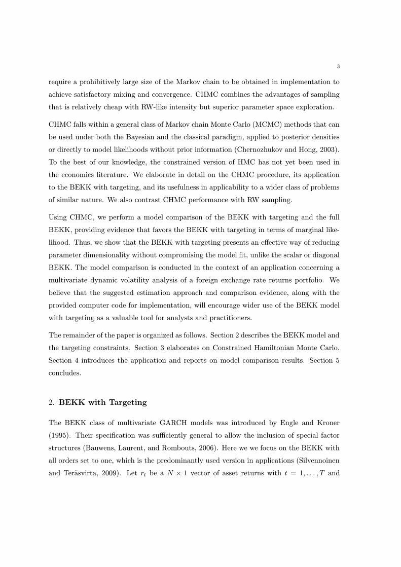
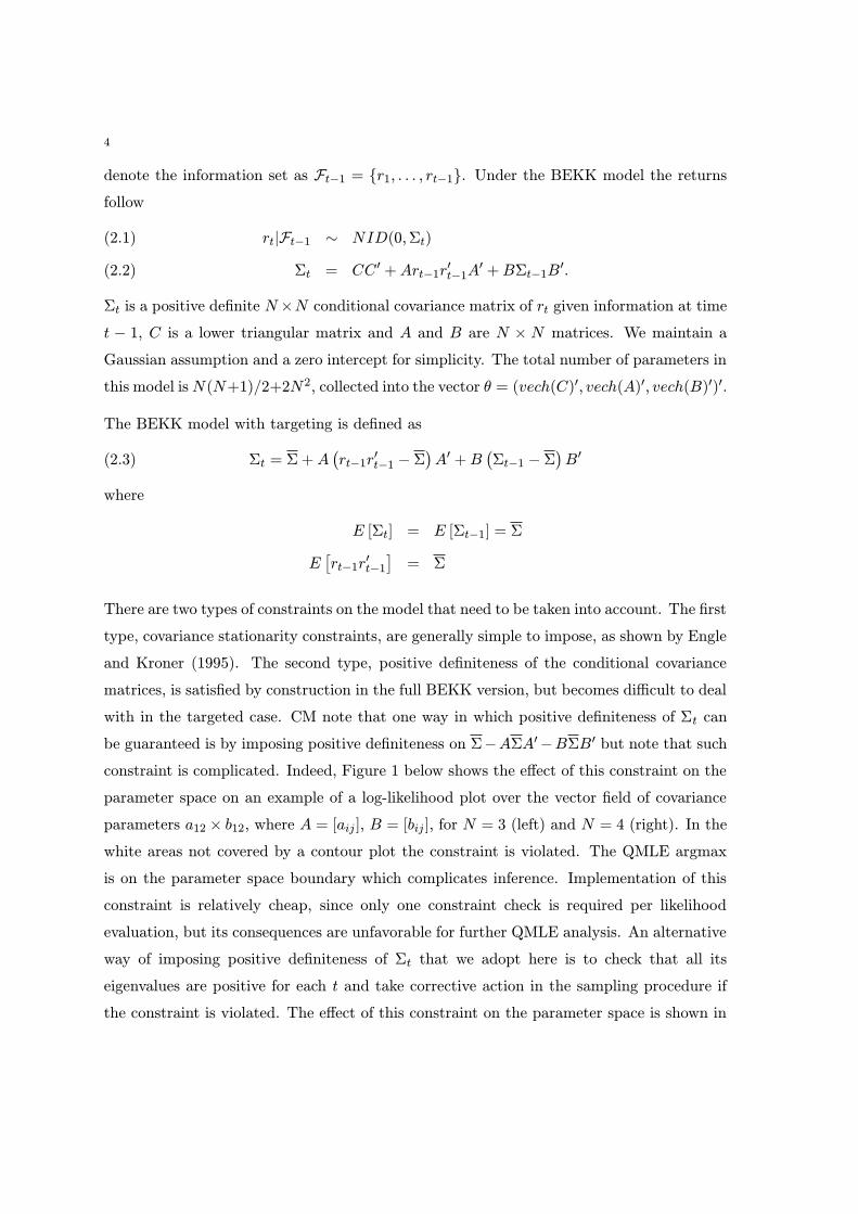
There are two types of constraints on the model that need to be taken into account. The first

type, covariance stationarity constraints, are generally simple to impose, as shown by Engle

and Kroner (1995). The second type, positive definiteness of the conditional covariance

matrices, is satisfied by construction in the full BEKK version, but becomes difficult to deal

with in the targeted case. CM note that one way in which positive definiteness of Σt can

be guaranteed is by imposing positive definiteness on Σ−AΣA′−BΣB′ but note that such

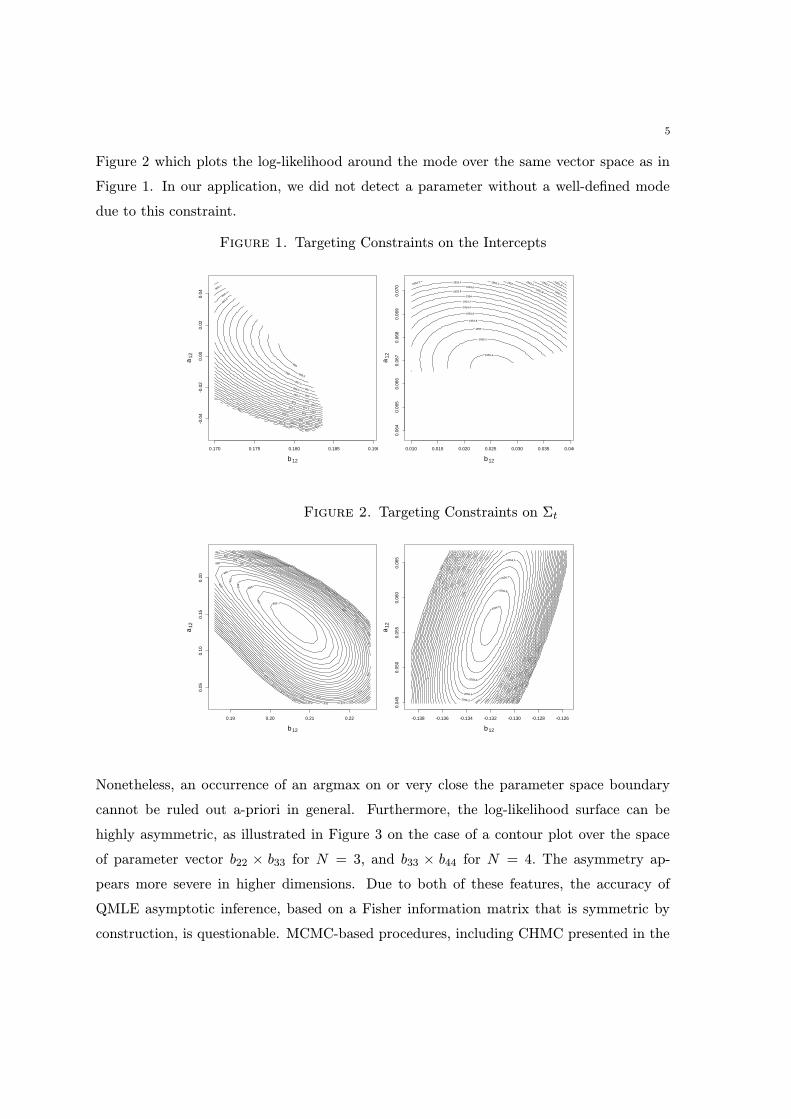
constraint is complicated. Indeed, Figure 1 below shows the effect of this constraint on the

parameter space on an example of a log-likelihood plot over the vector field of covariance

parameters a12 × b12, where A = [aij ], B = [bij ], for N = 3 (left) and N = 4 (right). In the

white areas not covered by a contour plot the constraint is violated. The QMLE argmax

is on the parameter space boundary which complicates inference. Implementation of this

constraint is relatively cheap, since only one constraint check is required per likelihood

evaluation, but its consequences are unfavorable for further QMLE analysis. An alternative

way of imposing positive definiteness of Σt that we adopt here is to check that all its

eigenvalues are positive for each t and take corrective action in the sampling procedure if

the constraint is violated. The effect of this constraint on the parameter space is shown in

5

Figure 2 which plots the log-likelihood around the mode over the same vector space as in

Figure 1. In our application, we did not detect a parameter without a well-defined mode

due to this constraint.

Figure 1. Targeting Constraints on the Intercepts

b12

a12

857

857 857

857.5 858

858.5 859

859.5

860

860.5

861

861.5

862

862.5 863

863

863.5

864

864

864.5

864.5

865

865.5 866

866.5 867

867.5

868 868.5

869

0.170 0.175 0.180 0.185 0.190

-0.0

4-0

.02

0.00

0.02

0.04

b12

a12

1951.8

1952.2

1952.4

1952.6

1952.8

1953 1953.2 1953.2 1953.4

1953.6

1953.8

1954

1954.2

1954.4

1954.6

1954.8

1955

1955.2

1955.4

0.010 0.015 0.020 0.025 0.030 0.035 0.040

0.06

40.

065

0.06

60.

067

0.06

80.

069

0.07

0

Figure 2. Targeting Constraints on Σt

b12

a12

870

870

871

871

872

872

872

873

873

874

874

875

875

875 876

876

876

877

877

878

878

879

879

880

880

881 882

883

884 885

886 887 888

889

890

891

892 893

894 895

0.19 0.20 0.21 0.22

0.05

0.10

0.15

0.20

b12

a12

205

4

205

4

205

4.1

205

4.1

205

4.2

205

4.2

205

4.3

205

4.3

205

4.4

205

4.4

205

4.5

205

4.5

205

4.6

205

4.6

205

4.7

205

4.7

205

4.8

205

4.8

205

4.9

205

4.9

205

5

205

5

205

5.1

205

5.1

205

5.2

205

5.2

205

5.3

205

5.3

205

5.4

205

5.4

205

5.5

205

5.5

205

5.6

205

5.6

205

5.7

205

5.7

205

5.8

205

5.8

205

5.9

205

5.9

205

6

205

6 2

056.

1

205

6.1

205

6.2

2056.2 2056.3

2056.4

2056.5

2056.6

2056.7

2056.8

2056.9

-0.138 -0.136 -0.134 -0.132 -0.130 -0.128 -0.126

0.04

50.

050

0.05

50.

060

0.06

5

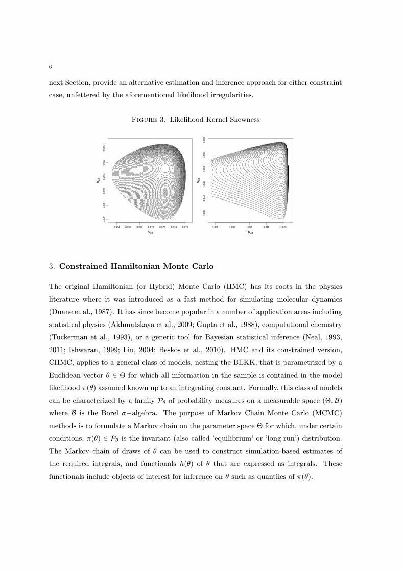
Nonetheless, an occurrence of an argmax on or very close the parameter space boundary

cannot be ruled out a-priori in general. Furthermore, the log-likelihood surface can be

highly asymmetric, as illustrated in Figure 3 on the case of a contour plot over the space

of parameter vector b22 × b33 for N = 3, and b33 × b44 for N = 4. The asymmetry ap-

pears more severe in higher dimensions. Due to both of these features, the accuracy of

QMLE asymptotic inference, based on a Fisher information matrix that is symmetric by

construction, is questionable. MCMC-based procedures, including CHMC presented in the

6

next Section, provide an alternative estimation and inference approach for either constraint

case, unfettered by the aforementioned likelihood irregularities.

Figure 3. Likelihood Kernel Skewness

b33

b22

850

851

852 853

854 855

856

857 858 859

860 861

862

863

864 865

866

867

868

869 870

871

872 873

874

875

876

877 878

879 880

881

882

883

884

885

886

887

888

889

890

891

892

893

894

895

0.964 0.966 0.968 0.970 0.972 0.974 0.976

0.97

00.

975

0.98

00.

985

0.99

00.

995

b44

b33

1905

1905

190

5

1910

1910

1915

1915

1920

1920

1925

1925

1930

1930

1935

1935

1940

1945

1950

1955

1960

1965

1970

1975 1980

1985

1990

1995

2000

2005

2010

2015

2020

2025

2030

2035

2040

2045

2050

2055

1.000 1.005 1.010 1.015 1.020

1.03

51.

040

1.04

51.

050

1.05

51.

060

3. Constrained Hamiltonian Monte Carlo

The original Hamiltonian (or Hybrid) Monte Carlo (HMC) has its roots in the physics

literature where it was introduced as a fast method for simulating molecular dynamics

(Duane et al., 1987). It has since become popular in a number of application areas including

statistical physics (Akhmatskaya et al., 2009; Gupta et al., 1988), computational chemistry

(Tuckerman et al., 1993), or a generic tool for Bayesian statistical inference (Neal, 1993,

2011; Ishwaran, 1999; Liu, 2004; Beskos et al., 2010). HMC and its constrained version,

CHMC, applies to a general class of models, nesting the BEKK, that is parametrized by a

Euclidean vector θ ∈ Θ for which all information in the sample is contained in the model

likelihood π(θ) assumed known up to an integrating constant. Formally, this class of models

can be characterized by a family Pθ of probability measures on a measurable space (Θ,B)

where B is the Borel σ−algebra. The purpose of Markov Chain Monte Carlo (MCMC)

methods is to formulate a Markov chain on the parameter space Θ for which, under certain

conditions, π(θ) ∈ Pθ is the invariant (also called ’equilibrium’ or ’long-run’) distribution.

The Markov chain of draws of θ can be used to construct simulation-based estimates of

the required integrals, and functionals h(θ) of θ that are expressed as integrals. These

functionals include objects of interest for inference on θ such as quantiles of π(θ).

7

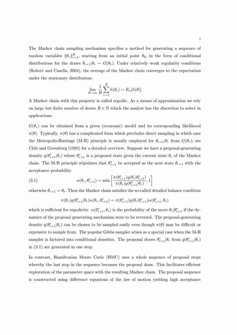
The Markov chain sampling mechanism specifies a method for generating a sequence of

random variables {θr}Rr=1, starting from an initial point θ0, in the form of conditional

distributions for the draws θr+1|θr ∼ G(θr). Under relatively weak regularity conditions

(Robert and Casella, 2004), the average of the Markov chain converges to the expectation

under the stationary distribution:

limR→∞

1

R

R∑

r=1

h(θr) = Eπ[h(θ)]

A Markov chain with this property is called ergodic. As a means of approximation we rely

on large but finite number of draws R ∈ N which the analyst has the discretion to select in

applications.

G(θr) can be obtained from a given (economic) model and its corresponding likelihood

π(θ). Typically, π(θ) has a complicated form which precludes direct sampling in which case

the Metropolis-Hastings (M-H) principle is usually employed for θr+1|θr from G(θr); see

Chib and Greenberg (1995) for a detailed overview. Suppose we have a proposal-generating

density q(θ∗r+1|θr) where θ∗r+1 is a proposed state given the current state θr of the Markov

chain. The M-H principle stipulates that θ∗r+1 be accepted as the next state θr+1 with the

acceptance probability

(3.1) α(θr, θ∗r+1) = min

[π(θ∗r+1)q(θr|θ

∗r+1)

π(θr)q(θ∗r+1|θr), 1

]

otherwise θr+1 = θr. Then the Markov chain satisfies the so-called detailed balance condition

π(θr)q(θ∗r+1|θr)α(θr, θ

∗r+1) = π(θ

∗r+1)q(θr|θ

∗r+1)α(θ

∗r+1, θr)

which is sufficient for ergodicity. α(θ∗r+1, θr) is the probability of the move θr|θ∗r+1 if the dy-

namics of the proposal generating mechanism were to be reversed. The proposal-generating

density q(θ∗r+1|θr) can be chosen to be sampled easily even though π(θ) may be difficult or

expensive to sample from. The popular Gibbs sampler arises as a special case when the M-H

sampler is factored into conditional densities. The proposal draws θ∗r+1|θr from q(θ∗r+1|θr)

in (3.1) are generated in one step.

In contrast, Hamiltonian Monte Carlo (HMC) uses a whole sequence of proposal steps

whereby the last step in the sequence becomes the proposal draw. This facilitates efficient

exploration of the parameter space with the resulting Markov chain. The proposal sequence

is constructed using difference equations of the law of motion yielding high acceptance

8

probability even for distant proposals. The parameter space Θ is augmented with a set

of independent auxiliary stochastic parameters γ ∈ Γ that fulfill a supplementary role in

the proposal algorithm, facilitating the directional guidance of the proposal mechanism.

The proposal sequence takes the form {θkr , γkr }Lk=1 starting from the current state (θr, γr) =

(θ0r , γ0r ) and yielding a proposal (θr, γr) = (θ

Lr , γ

Lr ). The detailed balance is then satisfied

using the acceptance probability

(3.2) α(θr, γr; θ∗r+1, γ

∗r+1) = min

[π(θ∗r+1, γ

∗r+1)q(θr, γr|θ

∗r+1, γ

∗r+1)

π(θr, γr)q(θ∗r+1, γ∗r+1|θr, γr)

, 1

]

In CHMC, constraints are incorporated into the HMC proposal mechanism via ”hard walls”

representing a barrier against which the proposal sequence, simulating a particle movement,

bounces off elastically. Constraints thus do not provide grounds for proposal rejection,

eliminating any associated redundancies. Heuristically, the constraint is checked at each

step of the proposal sequence and if it is violated then the trajectory of the sequence is

reflected off the hard wall posed by the constraint. This facilitates efficient exploration of

the parameter space even in the presence of highly complex parameter constraints. We

further synthesize the technical principles of CHMC in a generally accessible form in the

Appendix A. In the next Section we apply CHMC to the task of model comparison of the

full BEKK and the BEKK with targeting.

4. Application and Model Comparison

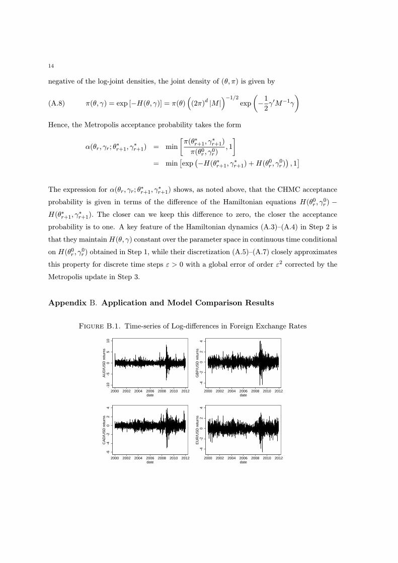
The model comparison is performed in the context of an empirical application with data on

percent log-differences of foreign exchange spot rates for AUD/USD, GBP/USD, CAD/USD,

and EUR/USD, from 2000/01/04 to 2011/12/30, total of T = 3, 009 observations. We con-

sider cases with two, three and four variables (N = 2, 3, 4) with data used in the order

presented. The associated parameter dimensionality for the full BEKK is 11, 24, and 42,

and for the BEKK with targeting 8, 18, and 32, respectively. A time series plot of the

four series is shown in Figure B.1 and summary statistics are provided in Table B.1 in

Appendix B. The sample mean for all series is close to 0 and skewness is small. The sample

correlations indicate that all series tend to move together.

9

For identification, the diagonal elements of C and the first element of both A and B are

restricted to be positive (Engle and Kroner, 1995). All priors, other than the model iden-

tification conditions, are set to be diffuse. In the implementation, we utilize the analytical

expressions for the gradient of the BEKK log-likelihood from Hafner and Herwartz (2008),

which in the case of the BEKK with targeting is subject to the targeting constraints (2.3).

Although numerical estimates of the gradients could also be used in forming the proposals,

evaluation of analytical expressions increases the implementation speed. The initial Σ1 in

the GARCH recursion is set to the sample covariance. Starting from the modal parameter

values we collect a total of 50, 000 posterior draws for inference, with 5, 000 burnin section.

The length of the proposal sequence was set to L = 50, 30, 20 for the cases N = 2, 3, 4

respectively, and the stepsize ε tuned to achieve acceptance rates close to 0.8.

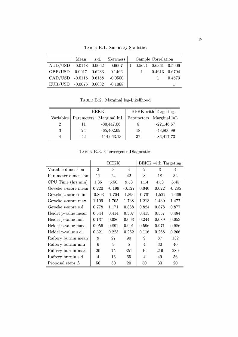
Table B.2 reports model comparison results of the full BEKK and BEKK with targeting in

terms of marginal log-likelihood (Gelfend and Dey, 1994; Geweke, 2005). Since all parame-

ters are integrated out, marginal likelihood does not explicitly depend on the dimensionality

of the parameter space and hence is suitable for comparison of models with different dimen-

sions. In all cases, N = 2, 3, 4, the evidence strongly favors the BEKK model with targeting

over the full BEKK model, and this effect increases with dimensionality of variables N.

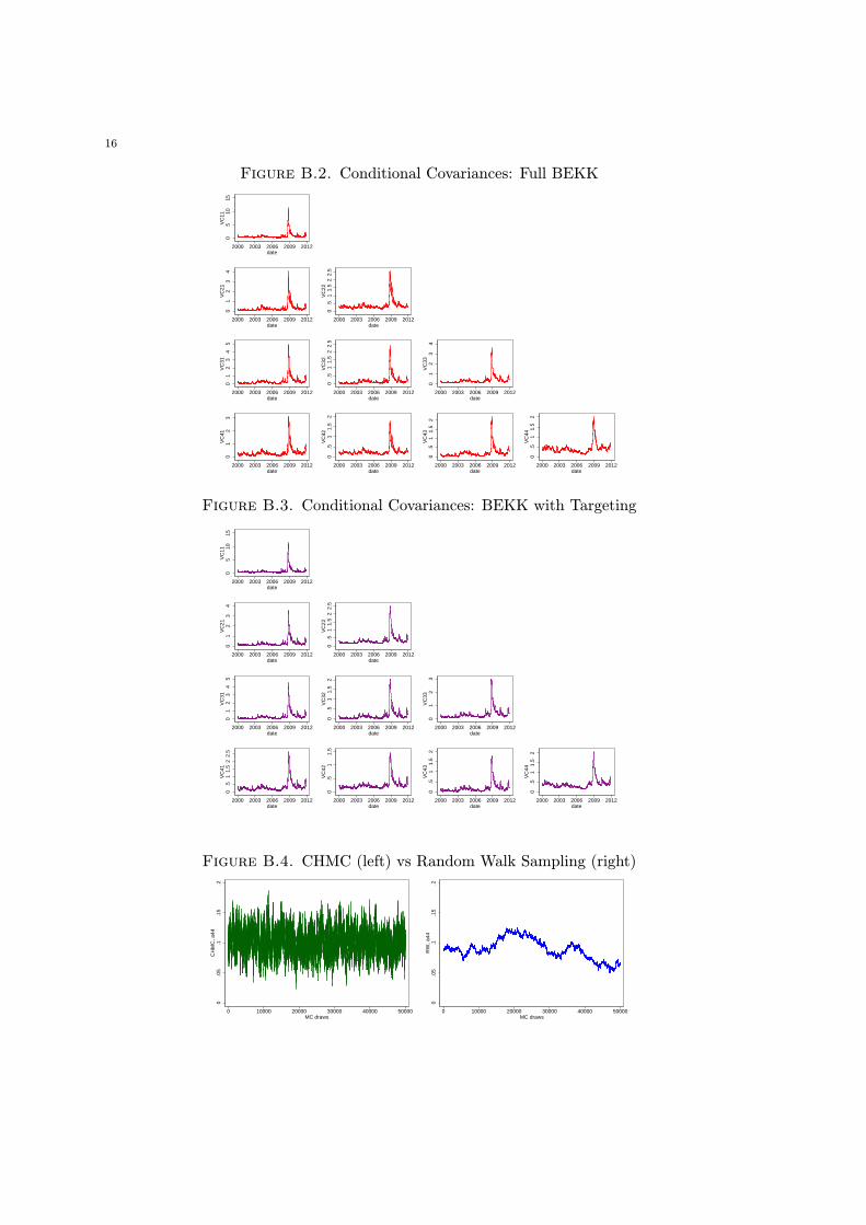
The evolution of the mean of the conditional covariances over time is presented in Figure

B.2 for the full BEKK, and in Figure B.3 for the BEKK with targeting, in four variables.

Both plots are virtually identical when examined closely, indicating a minimal loss of model

prediction capability as a result of targeting.

Markov chain convergence diagnostics, obtained using the R package coda, for both models

and variable dimensions are reported in Table B.3 confirming the validity of model inference

and comparison. All chains have converged within the burnin section, as evidenced by

the reported z-scores (mean, minimum, maximum, and standard deviation) of the Geweke

(1992) convergence test standardized z-score and p-values of the Heidelberger and Welch

(1983) stationary distribution test. The Raftery burnin control diagnostic (Raftery and

Lewis, 1995) confirms the sufficiency of the length of the burnin section. The CPU run

time, also reported in Table B.3, took in the order of hours and was virtually equivalent to

the wall-clock run time. All chains were obtained using fortran code with Intel compiler on

a 2.8 GHz Unix machine.

10

The advantages of HMC-based procedures over random walk (RW) sampling have been well

documented (Neal 2011; Pakman and Paninski 2012). We illustrate the CHMC versus RW

comparison in Figure B.4, showing the trace plot of the Markov chain for the conditional

variance parameter a44, in the BEKK with targeting, with 4 variables and 32 parameters.

The CHMC trace (left) mixes very well, exploring the tails of the likelihood kernel, while the

RW trace (right) stays within a relatively narrow band with minimal tail exploration and

without any signs of convergence. Overall, our results support the use of the BEKK with

targeting, and CHMC provides a suitable method to sample effectively from its likelihood

kernel with nonlinear constraints.

5. Conclusions

In this paper we suggest an effective approach for estimation and inference on the BEKK

GARCH model with targeting. The approach is based on Constrained Hamiltonian Monte

Carlo (CHMC), a recent statistical technique devised to handle nonlinear constraints in

the context of relatively costly and irregular likelihoods. Based on a model comparison

with the unrestricted version of the BEKK we present evidence favoring the BEKK with

targeting in terms of marginal likelihood. Due to its potential and applicability to similar

types of problems, we detail CHMC in a generally accessible form, and provide computer

code for its implementation. We also provide a comparison of the CHMC and random walk

sampling. We believe that the elaborated estimation approach and comparison evidence

will encourage wider use of both the BEKK model with targeting and CHMC as valuable

tools for analysts and practitioners.

Appendix A. Statistical Properties of Constrained Hamiltonian Monte Carlo

In this Section we provide the stochastic background for CHMC. This synthesis is based on

previously published material (Neal 2011; Burda and Maheu, 2012; and references therein).

However, the bulk of literature presenting HMC methods does so in terms of the physical

laws of motion based on preservation of total energy in the phase-space. Here we take a

fully stochastic perspective familiar to the applied econometrician. The CHMC principle is

thus presented in terms of the joint density over the augmented parameter space leading to

a Metropolis acceptance probability update.

11

A.1. CHMC Principle

Consider a vector of parameters of interest θ ∈ Rd distributed according to the density

kernel π(θ). Let γ ∈ Rd denote a vector of auxiliary parameters with γ ∼ Φ(γ; 0,M)

where Φ denotes the Gaussian distribution with mean vector 0 and covariance matrix M ,

independent of θ. M can be either set to the identity matrix or to a covariance matrix

estimated by the inverse of the Fisher information matrix around the mode, as we do in

our implementation. Denote the joint density of (θ, γ) by π(θ, γ). Denote the constraint on

the parameter space by a density kernel exp (Cr(θ)) where

Cr(θ) =

{0 if the constraint is satisfied

Cr > 0 s.t. limr→∞Cr =∞ if the constraint is violated

Then the negative of the logarithm of the joint density of (θ, γ) is given by the constrained

Hamiltonian equation1

(A.1) H(θ, γ) = −Cr(θ)− lnπ(θ) +1

2ln((2π)d |M |

)+1

2γ′M−1γ

Constrained Hamiltonian Monte Carlo (CHMC) is formulated in the following steps:

(1) Draw an initial auxiliary parameter vector γ0r ∼ Φ(γ; 0,M);

(2) Transition from (θr, γr) to (θLr , γ

Lr ) = (θ

∗r+1, γ

∗r+1) according to the constrained

Hamiltonian dynamics;

(3) Accept (θ∗r+1, γ∗r+1) with probability

(A.2) α(θr, γr; θ∗r+1, γ

∗r+1) = min

[exp

(−H(θ∗r+1, γ

∗r+1) +H(θ

0r , γ

0r )), 1],

otherwise keep (θr, γr) as the next MC draw.

The constraints on the parameter space Θ are reflected in Step 2. We will now describe

each step in detail.

Step 1 provides a stochastic initialization of the system akin to a RW draw in order to

make the resulting Markov chain {(θr, γr)}Rr=1 irreducible and aperiodic (Ishwaran, 1999).

In contrast to RW, this so-called refreshment move is performed on the auxiliary variable γ

1In the physics literature, θ denotes the position (or state) variable and − lnπ(θ) describes its potential

energy, while γ is the momentum variable with kinetic energy γ′M−1γ/2, yielding the total energy H(θ, γ)

of the system, up to a constant of proportionality. M is a constant, symmetric, positive-definite ”mass”

matrix.

12

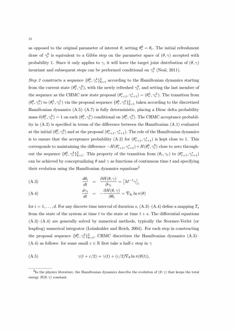
as opposed to the original parameter of interest θ, setting θ0r = θr. The initial refreshment

draw of γ0r is equivalent to a Gibbs step on the parameter space of (θ, γ) accepted with

probability 1. Since it only applies to γ, it will leave the target joint distribution of (θ, γ)

invariant and subsequent steps can be performed conditional on γ0r (Neal, 2011).

Step 2 constructs a sequence {θkr , γkr }Lk=1 according to the Hamiltonian dynamics starting

from the current state (θ0r , γ0r ), with the newly refreshed γ

0r , and setting the last member of

the sequence as the CHMC new state proposal (θ∗r+1, γ∗r+1) = (θ

Lr , γ

Lr ). The transition from

(θ0r , γ0r ) to (θ

Lr , γ

Lr ) via the proposal sequence {θ

kr , γ

kr }Lk=1 taken according to the discretized

Hamiltonian dynamics (A.5)–(A.7) is fully deterministic, placing a Dirac delta probability

mass δ(θkr , γkr ) = 1 on each (θ

kr , γ

kr ) conditional on (θ

0r , γ

0r ). The CHMC acceptance probabil-

ity in (A.2) is specified in terms of the difference between the Hamiltonian (A.1) evaluated

at the initial (θ0r , γ0r ) and at the proposal (θ

∗r+1, γ

∗r+1). The role of the Hamiltonian dynamics

is to ensure that the acceptance probability (A.2) for (θ∗r+1, γ∗r+1) is kept close to 1. This

corresponds to maintaining the difference −H(θ∗r+1, γ∗r+1)+H(θ

0r , γ

0r ) close to zero through-

out the sequence {θkr , γkr }Lk=1. This property of the transition from (θr, γr) to (θ

∗r+1, γ

∗r+1)

can be achieved by conceptualizing θ and γ as functions of continuous time t and specifying

their evolution using the Hamiltonian dynamics equations2

dθi

dt=∂H(θ, γ)

∂γi=[M−1γ

]i

(A.3)

dγi

dt= −

∂H(θ, γ)

∂θi= ∇θi lnπ(θ)(A.4)

for i = 1, . . . , d. For any discrete time interval of duration s, (A.3)–(A.4) define a mapping Ts

from the state of the system at time t to the state at time t+ s. The differential equations

(A.3)–(A.4) are generally solved by numerical methods, typically the Stormer-Verlet (or

leapfrog) numerical integrator (Leimkuhler and Reich, 2004). For each step in constructing

the proposal sequence {θkr , γkr }Lk=1, CHMC discretizes the Hamiltonian dynamics (A.3)–

(A.4) as follows: for some small ε ∈ R first take a half-ε step in γ

(A.5) γ(t+ ε/2) = γ(t) + (ε/2)∇θ lnπ(θ(t)),

2In the physics literature, the Hamiltonian dynamics describe the evolution of (θ, γ) that keeps the total

energy H(θ, γ) constant.

13

then take a full ε step in θ

(A.6) θ(t+ ε) = θ(t) + εM−1γ(t+ ε/2),

check the constraint at θ(t+ε) for each dimension i of θ, if for any i the constraint is violated

then set γi(t+ ε/2) = −γi(t+ ε/2) reversing the proposal dynamics and take further steps

in θi until the constraint is satisfied, then finish with another half-ε step in γ

(A.7) γ(t+ ε) = γ(t+ ε/2) + (ε/2)∇θ lnπ(θ(t+ ε)).

Intuitively, the proposal trajectory bounces off the ”walls” given by the constraint. Since

a move in γ only occurs conditional on θ for which the constraint is satisfied in which case

Cr(θ) = 0, and the move in θ only depends on ∂H(θ, γ)/∂γi which does not involve Cr(θ),

the exact functional form of Cr(θ) is inconsequential as long as it is differentiable in θ to

define valid Hamiltonian dynamics.

From the statistical perspective, γ plays the role of an auxiliary variable that parametrizes

(a functional of) π(θ) providing it with an additional degree of flexibility to maintain the

acceptance probability close to one for every k. Even though ln π(θkr ) can deviate substan-

tially from ln π(θ0r), resulting in favorable mixing for θ, the additional terms in γ in (A.1)

compensate for this deviation maintaining the overall level of H(θkr , γkr ) close to constant

over k = 1, . . . , L when used in accordance with (A.5)–(A.7), since ∂H(θ,γ)∂γiand ∂H(θ,γ)∂θi

enter

with the opposite signs in (A.3)–(A.4). In contrast, without the additional parametrization

with γ, if only ln π(θkr ) were to be used in the proposal mechanism as is the case in RW

style samplers, the M-H acceptance probability would often drop to zero relatively quickly.

Step 3 applies a Metropolis correction to the proposal (θ∗r+1, γ∗r+1). In continuous time, or

for ε → 0, (A.3)–(A.4) would keep −H(θ∗r+1, γ∗r+1) + H(θr, γr) = 0 exactly resulting in

α(θr, θ∗r+1) = 1 but for discrete ε > 0, in general, −H(θ

∗, γ∗) + H(θ, γ) 6= 0 necessitating

the Metropolis step.

The system (A.5)–(A.7) is time reversible and symmetric in (θ, γ), which implies that the

forward and reverse transition probabilities q(θLr , γLr |θ0r , γ

0r ) and q(θ

0r , γ

0r |θLr , γ

Lr ) are equal:

this simplifies the Metropolis-Hastings acceptance ratio in (3.2) to the Metropolis form

π(θ∗r+1, γ∗r+1)/π(θ

0r , γ

0r ). From the definition of the Hamiltonian H(θ, γ) in (A.1) as the

14

negative of the log-joint densities, the joint density of (θ, π) is given by

(A.8) π(θ, γ) = exp [−H(θ, γ)] = π(θ)((2π)d |M |

)−1/2exp

(

−1

2γ′M−1γ

)

Hence, the Metropolis acceptance probability takes the form

α(θr, γr; θ∗r+1, γ

∗r+1) = min

[π(θ∗r+1, γ

∗r+1)

π(θ0r , γ0r ), 1

]

= min[exp

(−H(θ∗r+1, γ

∗r+1) +H(θ

0r , γ

0r )), 1]

The expression for α(θr, γr; θ∗r+1, γ

∗r+1) shows, as noted above, that the CHMC acceptance

probability is given in terms of the difference of the Hamiltonian equations H(θ0r , γ0r ) −

H(θ∗r+1, γ∗r+1). The closer can we keep this difference to zero, the closer the acceptance

probability is to one. A key feature of the Hamiltonian dynamics (A.3)–(A.4) in Step 2 is

that they maintainH(θ, γ) constant over the parameter space in continuous time conditional

on H(θ0r , γ0r ) obtained in Step 1, while their discretization (A.5)–(A.7) closely approximates

this property for discrete time steps ε > 0 with a global error of order ε2 corrected by the

Metropolis update in Step 3.

Appendix B. Application and Model Comparison Results

Figure B.1. Time-series of Log-differences in Foreign Exchange Rates

-10

-50

510

AU

D/U

SD

ret

urns

2000 2002 2004 2006 2008 2010 2012date

-4-2

02

4G

BP

/US

D r

etur

ns

2000 2002 2004 2006 2008 2010 2012date

-6-4

-20

24

CA

D/U

SD

ret

urns

2000 2002 2004 2006 2008 2010 2012date

-4-2

02

4E

UR

/US

D r

etur

ns

2000 2002 2004 2006 2008 2010 2012date

15

Table B.1. Summary Statistics

Mean s.d. Skewness Sample Correlation

AUD/USD -0.0148 0.9062 0.6607 1 0.5621 0.6361 0.5906

GBP/USD 0.0017 0.6233 0.1466 1 0.4613 0.6794

CAD/USD -0.0118 0.6188 -0.0500 1 0.4873

EUR/USD -0.0076 0.6682 -0.1068 1

Table B.2. Marginal log-Likelihood

BEKK BEKK with Targeting

Variables Parameters Marginal lnL Parameters Marginal lnL

2 11 -30,447.06 8 -22,146.67

3 24 -65,402.69 18 -48,806.99

4 42 -114,063.13 32 -86,417.73

Table B.3. Convergence Diagnostics

BEKK BEKK with Targeting

Variable dimension 2 3 4 2 3 4

Parameter dimension 11 24 42 8 18 32

CPU Time (hrs:min) 1:35 5:50 9:53 1:14 4:53 6:45

Geweke z-score mean 0.220 -0.199 -0.127 0.040 0.022 -0.285

Geweke z-score min -0.803 -1.704 -1.896 -0.761 -1.522 -1.669

Geweke z-score max 1.109 1.705 1.738 1.213 1.430 1.477

Geweke z-score s.d. 0.778 1.171 0.868 0.824 0.878 0.877

Heidel p-value mean 0.544 0.414 0.307 0.415 0.537 0.484

Heidel p-value min 0.137 0.086 0.063 0.244 0.089 0.053

Heidel p-value max 0.956 0.892 0.991 0.596 0.971 0.986

Heidel p-value s.d. 0.321 0.223 0.262 0.116 0.268 0.266

Raftery burnin mean 9 27 90 9 87 132

Raftery burnin min 6 9 5 4 30 40

Raftery burnin max 20 75 351 16 216 280

Raftery burnin s.d. 4 16 65 4 49 56

Proposal steps L 50 30 20 50 30 20

16

Figure B.2. Conditional Covariances: Full BEKK

05

1015

VC

11

2000 2003 2006 2009 2012date

01

23

4V

C21

2000 2003 2006 2009 2012date

01

23

45

VC

31

2000 2003 2006 2009 2012date

01

23

VC

41

2000 2003 2006 2009 2012date

0.5

11.

52

2.5

VC

222000 2003 2006 2009 2012

date0

.51

1.5

22.

5V

C32

2000 2003 2006 2009 2012date

0.5

11.

52

VC

42

2000 2003 2006 2009 2012date

01

23

4V

C33

2000 2003 2006 2009 2012date

0.5

11.

52

VC

43

2000 2003 2006 2009 2012date

0.5

11.

52

VC

44

2000 2003 2006 2009 2012date

Figure B.3. Conditional Covariances: BEKK with Targeting

05

1015

VC

11

2000 2003 2006 2009 2012date

01

23

4V

C21

2000 2003 2006 2009 2012date

01

23

45

VC

31

2000 2003 2006 2009 2012date

0.5

11.

52

2.5

VC

41

2000 2003 2006 2009 2012date

0.5

11.

52

2.5

VC

22

2000 2003 2006 2009 2012date

0.5

11.

52

VC

32

2000 2003 2006 2009 2012date

0.5

11.

5V

C42

2000 2003 2006 2009 2012date

01

23

VC

33

2000 2003 2006 2009 2012date

0.5

11.

52

VC

43

2000 2003 2006 2009 2012date

0.5

11.

52

VC

44

2000 2003 2006 2009 2012date

Figure B.4. CHMC (left) vs Random Walk Sampling (right)

0.0

5.1

.15

.2C

HM

C, a

44

0 10000 20000 30000 40000 50000MC draws

0.0

5.1

.15

.2R

W, a

44

0 10000 20000 30000 40000 50000MC draws

17

References

Aielli, G. P. (2011). Dynamic conditional correlation: On properties and estimation. Available at

http://papers.ssrn.com/sol3/papers.cfmabstract id=1507743, SSRN Working Paper,.

Akhmatskaya, E., N. Bou-Rabee, and S. Reich (2009). A comparison of generalized hybrid monte

carlo methods with and without momentum flip. Journal of Computational Physics 228 (6),

2256–2265.

Bauwens, L., S. Laurent, and J. V. K. Rombouts (2006). Multivariate garch models: a survey.

Journal of Applied Econometrics 21, 79–109.

Beskos, A., N. S. Pillai, G. O. Roberts, J. M. Sanz-Serna, and A. M. Stuart (2010). Optimal tuning

of the hybrid monte-carlo algorithm. Working paper, arxiv:1001.4460v1 [math.pr].

Billio, M. and M. Caporin (2009). A generalized dynamic conditional correlation model for portfolio

risk evaluation. Mathematics and Computers in Simulation 79 (8), 25662578.

Burda, M. and J. M. Maheu (2012). Bayesian adaptively updated hamiltonian monte carlo with

an application to high-dimensional BEKK GARCH models. Studies in Nonlinear Dynamics &

Econometrics, forthcoming.

Caporin, M. and M. McAleer (2012). Do we really need both BEKK and DCC? a tale of two

multivariate garch models. Journal of Economic Surveys 26 (4), 736751.

Chernozhukov, V. and H. Hong (2003). An MCMC approach to classical estimation. Journal of

Econometrics 115 (3), 293–346.

Chib, S. and E. Greenberg (1995). Understanding the metropolis-hastings algorithm. American

Statistician 49 (4), 327–335.

Ding, Z. and R. Engle (2001). Large scale conditional covariance matrix modeling, estimation and

testing. Academia Economic Papers 29, 157184.

Duane, S., A. Kennedy, B. Pendleton, and D. Roweth (1987). Hybrid monte carlo. Physics Letters

B 195 (2), 216–222.

Engle, R. F. (2002). Dynamic conditional correlation: A simple class of multivariate generalized

autoregressive conditional heteroskedasticity models. Journal of Business and Economic Statis-

tics 20, 339–350.

Engle, R. F. and K. F. Kroner (1995). Multivariate simultaneous generalized arch. Econometric

Theory 11 (1), 122–150.

Engle, R. F., N. Shephard, and K. Sheppard (2009). Fitting vast dimensional time-varying covariance

models. Available at SSRN: http://ssrn.com/abstract=1354497.

Gelfand, A. and D. Dey (1994). Bayesian model choice: Asymptotics and exact calculations. Journal

of the Royal Statistical Society, Ser. B 56, 501–514.

Geweke, J. (1992). Evaluating the accuracy of sampling-based approaches to calculating posterior

moments. In J. Bernado, J. O. Berger, A. Dawid, and A. Smith (Eds.), Bayesian Statistics 4.

Clarendon Press, Oxford, UK.

Geweke, J. (2005). Contemporary Bayesian Econometrics and Statistics. Hoboken, New Jersey:

Wiley.

18

Gupta, R., G. Kilcup, and S. Sharpe (1988). Tuning the hybrid monte carlo algorithm. Physical

Review D 38 (4), 1278–1287.

Hafner, C. M. and H. Herwartz (2008). Analytical quasi maximum likelihood inference in multivariate

volatility models. Metrika 67, 219–239.

Heidelberger, P. and P. Welch (1983). Simulation run length control in the presence of an initial

transient. Operations Research 31, 1109–44.

Ishwaran, H. (1999). Applications of hybrid monte carlo to generalized linear models: Quasicomplete

separation and neural networks. Journal of Computational and Graphical Statistics 8, 779–799.

Jin, X. and J. Maheu (2012). Modeling realized covariances and returns. forthcoming, Journal of

Financial Econometrics.

Leimkuhler, B. and S. Reich (2004). Simulating Hamiltonian Dynamics. Cambridge University

Press.

Liu, J. S. (2004). Monte Carlo Strategies in Scientific Computing. Springer Series in Statistics.

Neal, R. M. (1993). Probabilistic inference using markov chain monte carlo methods. Technical

report crg-tr-93-1, Dept. of Computer Science, University of Toronto.

Neal, R. M. (2011). Mcmc using hamiltonian dynamics. In S. Brooks, A. Gelman, G. Jones, and

X.-L. Meng (Eds.), Handbook of Markov Chain Monte Carlo. Chapman & Hall / CRC Press.

Pakman, A. and L. Paninski (2012). Exact hamiltonian monte carlo for truncated multivariate

gaussians. Available at http://arxiv.org/abs/1208.4118, Columbia University.

Plummer, M., N. Best, K. Cowles, K. Vines, D. Sarkar, and R. Almond (2012). The R package

coda. version 0.16-1.

Raftery, A. and S. Lewis (1995). The number of iterations, convergence diagnostics and generic

metropolis algorithms. In W. Gilks, D. Spiegelhalter, and S. Richardson (Eds.), Practical Markov

Chain Monte Carlo. London, U.K.: Chapman and Hall.

Robert, C. P. and G. Casella (2004). Monte Carlo statistical methods (Second ed.). New York:

Springer.

Silvennoinen, A. and T. Terasvirta (2009). Modeling multivariate autoregressive conditional het-

eroskedasticity with the double smooth transition conditional correlation garch model. Journal

of Financial Econometrics 7 (4), 373–411.

Tuckerman, M., B. Berne, G. Martyna, and M. Klein (1993). Efficient molecular dynamics and

hybrid monte carlo algorithms for path integrals. The Journal of Chemical Physics 99 (4), 2796–

2808.