Embed Size (px)
Citation preview
Constitutive Modelling of Soils under High Strain Rates Theoretical, Numerical, and Experimental Results
Prepared By: Kaiwen Xia (Ph.D.) Mohammadamin Jafari Patrick Paskalis Kanopoulos Yao Wei Department of Civil Engineering, University of Toronto, Toronto, Ontario PWGSC Contract Number: W7701-135578/001/QCL CSA: Grant McIntosh, Defence Scientist, 418-844-4000 ext. 4278
The scientific or technical validity of this Contract Report is entirely the responsibility of the Contractor and the contents do not necessarily have the approval or endorsement of the Department of National Defence of Canada.
Contract Report
DRDC-RDDC-2015-C071
March 2015

© Her Majesty the Queen in Right of Canada, as represented by the Minister of National Defence, 2015
© Sa Majesté la Reine (en droit du Canada), telle que représentée par le ministre de la Défense nationale,
2015
Numerical Modeling W7701-135578/001/QCL
A REPORT
PRESENTED TO DRDC VALCARTIER
March 31, 2015
CONSTITUTIVE MODELLING OF SOILS UNDER HIGH STRAIN RATES:
THEORETICAL, NUMERICAL, AND EXPERIMENTAL RESULTS
by
Kaiwen Xia (Ph.D.)
Mohammadamin Jafari
Patrick Paskalis Kanopoulos
Yao Wei
Department of Civil Engineering, University of Toronto
2015-03-31 Numerical Modeling W7701-135578/001/QCL
2
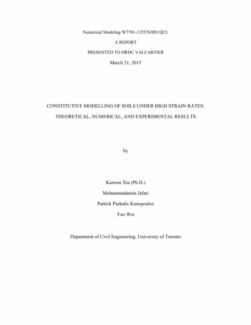
Abstract
The following report briefly outlines the concept of Perzyna-type viscoplasticity and its underlying constitutive equations that describe the nonlinear stress-strain relations of rate-dependant materials in the generalized tensor framework. Following the theoretical development, a numerical algorithm that computes the stress increment based on known a strain increment is presented. This algorithm is suitable for implementation into finite element codes (including hydrocodes such as LS-DYNA). Experimental stress-strain results from fine and coarse grained soils ranging from strain rates of 100 s-1 to 2100 s-1 are presented. The constitutive equations are calibrated against the experimental data using the Marquardt-Levenberg nonlinear optimisation algorithm. The material constants provided as a result of the calibration are suitable for implementation in hydrocodes, provided similar material types and conditions are being modelled over strain rates within the same orders of magnitude of the testing.
A three phase equation of state is presented both in the theoretical form and in a numerically appropriate pseudocode. The numerical code returns changes in pressure based on prescribed changes in volume, or computes an updated material bulk modulus. Parameters for the three phase model are derived from the literature for various sand types and degrees of saturation.
Finally, the constitutive model (both in the volumetric/deviator and deviator-only versions), and the three phase equation of state are implemented in FORTRAN77 source code and compiled as part of an LS-DYNA executable. Simulations are conducted in LS-DYNA and compared to readily available explosion experiments from the open literature. Simulated and experimental results show good agreement with each other.
2015-03-31 Numerical Modeling W7701-135578/001/QCL
3
Contents
Chapter 2: Numerical Implementation .................................................................................................... 7
Chapter 3: Experimental Procedures .................................................................................................... 11
3.1 Split Hopkinson Pressure Bar Method .................................................................................. 11
3.2 Physical properties of the sand used in the experiments ................................................... 12
3.3 Dynamic experimental results on dry sand .......................................................................... 14
3.4 Dynamic experimental results on saturated sand ............................................................... 15
3.5 Uniaxial strain tests in the quasi-static state ........................................................................ 16
Chapter 4: Calibration of the constitutive model .................................................................................. 17
4.1 Calibration of fine grained dry sand ....................................................................................... 17
4.2 Calibration of coarse grained dry sand ................................................................................. 17
4.3 Calibration of coarse grained saturated sand ...................................................................... 20
4.1 Calibration of fine grained saturated sand ............................................................................ 20
Chapter 5: Equation of State .............................................................................................................. 23
5.1 Three-Phase Equation of State .............................................................................................. 23
5.2 Numerical Implementation of the Equation of State ........................................................... 26
5.3 Suitable parameters for the equation of state ...................................................................... 29
Chapter 6: Numerical simulation ........................................................................................................ 30
6.1 Model Geometry and Parameters .......................................................................................... 30
6.2 Model results ............................................................................................................................. 35
Conclusion ................................................................................................................................................. 39
References ................................................................................................................................................ 40
Appendix A: Subroutine implementation in LS-DYNA ................................................................... 41
Appendix B: User defined constitutive model ................................................................................. 43
B.1 Deviatoric/Volumetric constitutive model source code and associated subroutines ..... 43
B.2 Deviatoric-only constitutive model source code .................................................................. 60
Appendix C: User defined equation of state model source code ................................................. 68
Appendix D: SHPB Experimental Results ....................................................................................... 73
Appendix E: EOS Parameter Estimation ......................................................................................... 89
Chapter 1: Theoretical Framework
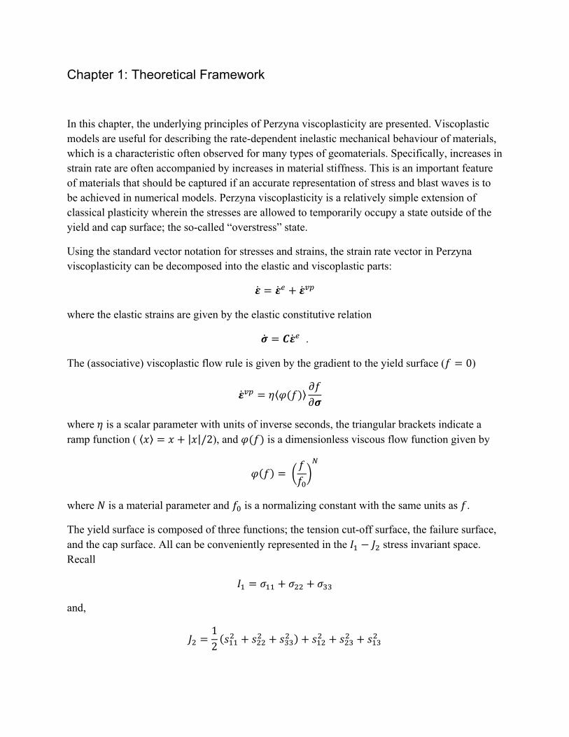
In this chapter, the underlying principles of Perzyna viscoplasticity are presented. Viscoplastic models are useful for describing the rate-dependent inelastic mechanical behaviour of materials, which is a characteristic often observed for many types of geomaterials. Specifically, increases in strain rate are often accompanied by increases in material stiffness. This is an important feature of materials that should be captured if an accurate representation of stress and blast waves is to be achieved in numerical models. Perzyna viscoplasticity is a relatively simple extension of classical plasticity wherein the stresses are allowed to temporarily occupy a state outside of the yield and cap surface; the so-called “overstress” state.
Using the standard vector notation for stresses and strains, the strain rate vector in Perzyna viscoplasticity can be decomposed into the elastic and viscoplastic parts:
where the elastic strains are given by the elastic constitutive relation
.
The (associative) viscoplastic flow rule is given by the gradient to the yield surface ( 0)
⟨ ⟩
where is a scalar parameter with units of inverse seconds, the triangular brackets indicate a ramp function ( ⟨ ⟩ | |/2), and is a dimensionless viscous flow function given by
where is a material parameter and is a normalizing constant with the same units as .
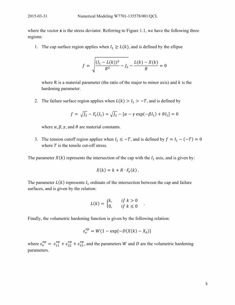
The yield surface is composed of three functions; the tension cut-off surface, the failure surface, and the cap surface. All can be conveniently represented in the stress invariant space. Recall
and,
12
2015-03-31 Numerical Modeling W7701-135578/001/QCL
5
where the vector is the stress deviator. Referring to Figure 1.1, we have the following three regions:
1. The cap surface region applies when , and is defined by the ellipse
0
where R is a material parameter (the ratio of the major to minor axis) and is the hardening parameter.
2. The failure surface region applies when , and is defined by
exp 0
where , , ,and are material constants.
3. The tension cutoff region applies when , and is defined by 0 where is the tensile cut-off stress.
The parameter represents the intersection of the cap with the axis, and is given by:
∙ . The parameter represents ordinate of the intersection between the cap and failure surfaces, and is given by the relation:
, 00, 0.
Finally, the volumetric hardening function is given by the following relation:
1 exp
where , and the parameters and are the volumetric hardening
parameters.
2015-03-31 Numerical Modeling W7701-135578/001/QCL
6
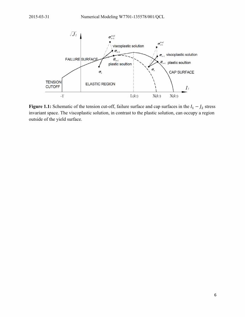
Figure 1.1: Schematic of the tension cut-off, failure surface and cap surfaces in the stress invariant space. The viscoplastic solution, in contrast to the plastic solution, can occupy a region outside of the yield surface.
2015-03-31 Numerical Modeling W7701-135578/001/QCL
7
Chapter 2: Numerical Implementation
Displacement based, explicitly integrated finite element codes require the computation of stresses as a function as assumed displacements (strains) at Gaussian points. It is therefore necessary to design an algorithm which can accurately return incremental stresses for given incremental states of strains over a known time step. The most common method in computational inelasticity of accomplishing this is the return-mapping algorithm, which is effectively a Newton-Rhapson approximation from an elastic predictor stress onto the yield surface (or, in the case of viscoplasticity, onto the appropriate overstressed state). The incremental stress and strain vectors are given by the following equations:
∆ ∆ ∆
∆ ∆ ∆ ∆ An Euler approximation of the total strain increment at time ∆ yields
∆ 1 ∆ ∆ ,0 1 where is the integration parameter. In the forgoing, a fully implicit approximation is used ( 1 , and in this case, the solution is unconditionally stable and the viscoplastic flow is determined by the gradient of the flow function only at time ∆ . Therefore, we have
∆ ∆ ∆ ⟨ ⟩∆ ∆
where ∆ is the plastic multiplier,
∆ ⟨ ⟩∆ . The problem is solved if the residual, , approaches zero during a local iteration:
∆∆
→ 0.
The stress increment can be rewritten in terms of the plastic multiplier ∆ ,
∆ ∆ ∆ .
2015-03-31 Numerical Modeling W7701-135578/001/QCL
8
In order to compute ∆ , a local Newton-Rhapson iteration is applied by taking the differential of the stress increment above for iteration :
: ∆ ∆ .
Using a pseudoelastic stiffness matrix, , we can represent by
: ∆
with,
∆ .
By differentiating the residual , the Newton-Rhapson iteration is expressed as
1∆
substituting into the equation for yields
1
with
∆1∆
.
To obtain an accurate estimate of the stress increment ∆ , several local iterations for should be applied until suitable convergence is obtained. A detailed process in pseudocode is provided in the following list, which based, with some modification, on the method proposed by Tong and Tuan (2007).
2015-03-31 Numerical Modeling W7701-135578/001/QCL
9
1. Compute the trial stresses based on the elastic stiffness: ∆ ∆
2. Check if stresses are outside the yield surface. If 0 and , ∆ go to step 3. If
0 and , ∆ go to step 5. If 0, return;
3. Assign the initial values before iteration:
∆ 0
∆
∆ ,∆∆
4. Loop for local iteration ,
i. Calculate pseudoelastic matrix , and variable
ii. Update ∆ , ∆ , according to
∆ ∆
∆ ∆ ∆
∆
∆
ln 1 ∆ /
*or, return elastic loading stresses if ∆ 0.99 to ensure non-singularity of
∆ from implicit solution of ∙
2015-03-31 Numerical Modeling W7701-135578/001/QCL
10
iii. Check for convergence, and if tolerance , return;
∆ , ∆
∆∆
5. Tensile regime, return corrected tensile stresses as follows:
i. If , ∆ and , ∆ , then
, ∆∆
, ∆ 1 ∆
, ∆ , ∆
ii. If , ∆ and , ∆ , then
, ∆∆
, ∆ 1 ∆
, ∆∆
, ∆ 1 ∆
iii. Return;
6. Return stresses and hardening parameter, end subroutine
It should be noted that in the user defined subroutines that have been implemented, an optional non-linear (exponential) elastic loading/unloading constitutive behaviour is provided. In this case, the tangential stiffness matrix is computed by means of the equations for bulk and shear moduli as:
exp
exp
where and have dimension of stress, has dimension of inverse stress, and has dimension of root inverse stress. Furthermore, and may be different in loading and unloading, where loading is defined as an increase in volumetric strain.
2015-03-31 Numerical Modeling W7701-135578/001/QCL
11
Chapter 3: Experimental Procedures
In this chapter, the experimental procedures are described in brief and the experimental results of the tests are summarised.
3.1 Split Hopkinson Pressure Bar Method
The method used to determine the physical behaviour of sand at high strain rates (from 102 to 104 s-1 was the split Hopkinson pressure bar (SHPB) method. In this method, the material sample is placed between an incident bar and a transmitted bar. A striker is launched towards the incident bar which initiates a stress wave that travels through the sample and into the transmitted bar. The impedance mismatch between the sample and steel bars results in a reflected and a transmitted wave. Comparisons of the incident, transmitted, and reflected waves, together with the simple theory of one dimensional wave propagation, allows the axial stress-strain history to be determined. Different maximum strains, and strain rates are achieved through variation of the striker velocity, and the type of pulse shaper used between the striker and the incident bar. Another important characteristic which should be observed during the course of the test is force balancing. Force balance is said to be achieved when the load history on each bar-material interface is equal at a given point in time. Inertial effects (the multiple internal propagation of stress waves in the sample) can be neglected if force balance is occurring, in other words, the material is deforming uniformly throughout during the test.
The typical SHPB setup was modified for the sand tests in order to achieve a uniaxial state of stress in the material. The sample strain histories can therefore be described as follows:
, 0.
The uniaxial state of strain was achieved by means of a thick steel sample holder which completely constrained the expansion of the material during the course of the tests.
For all dynamic tests conducted in the SHPB system, the sample was 5 mm in length and 25.4 mm in diameter (which is the same diameter as the bars). All bars and strikers were maraging steel with a density of 8.1 g/cm3, a Young’s modulus of 200 GPa, and a strength of 2.5 GPa. The striker bar was 30 cm long.
2015-03-31 Numerical Modeling W7701-135578/001/QCL
12
3.2 Physical properties of the sand used in the experiments
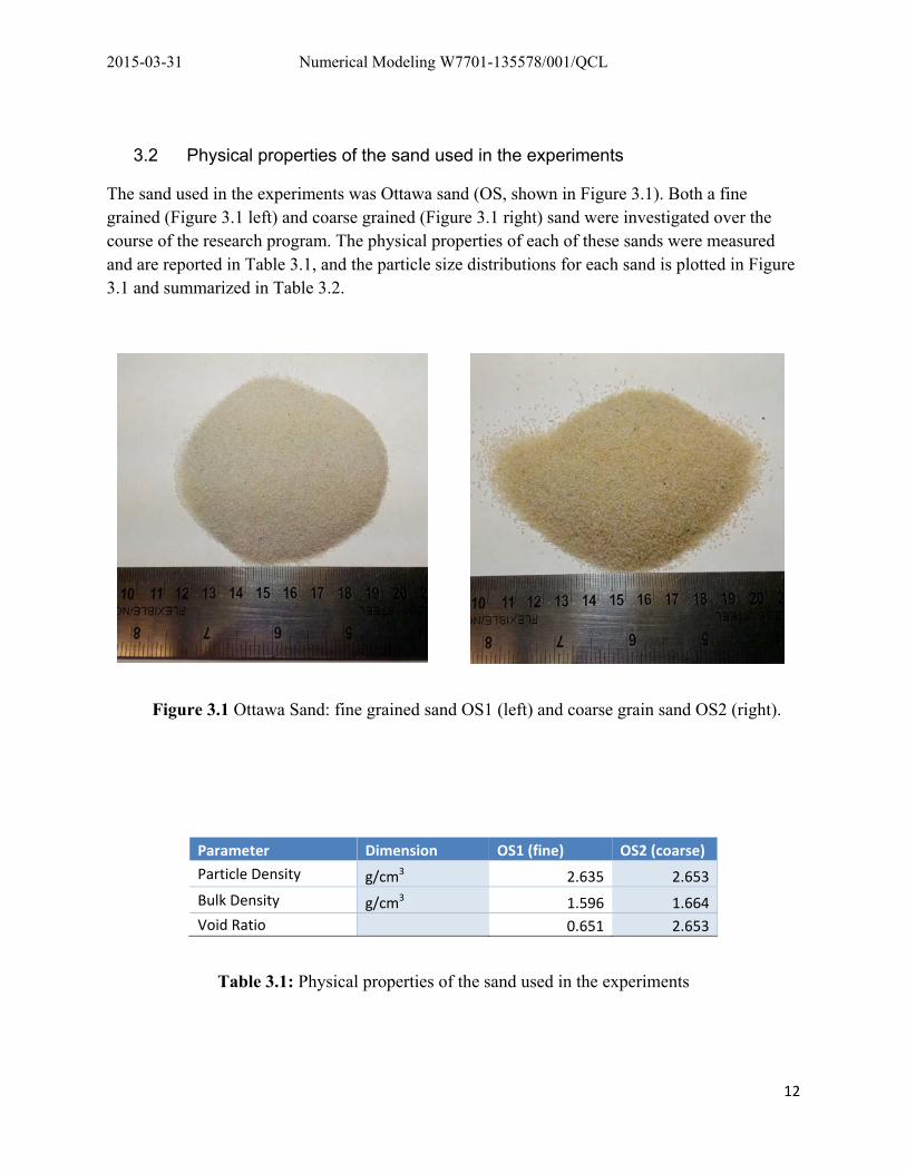
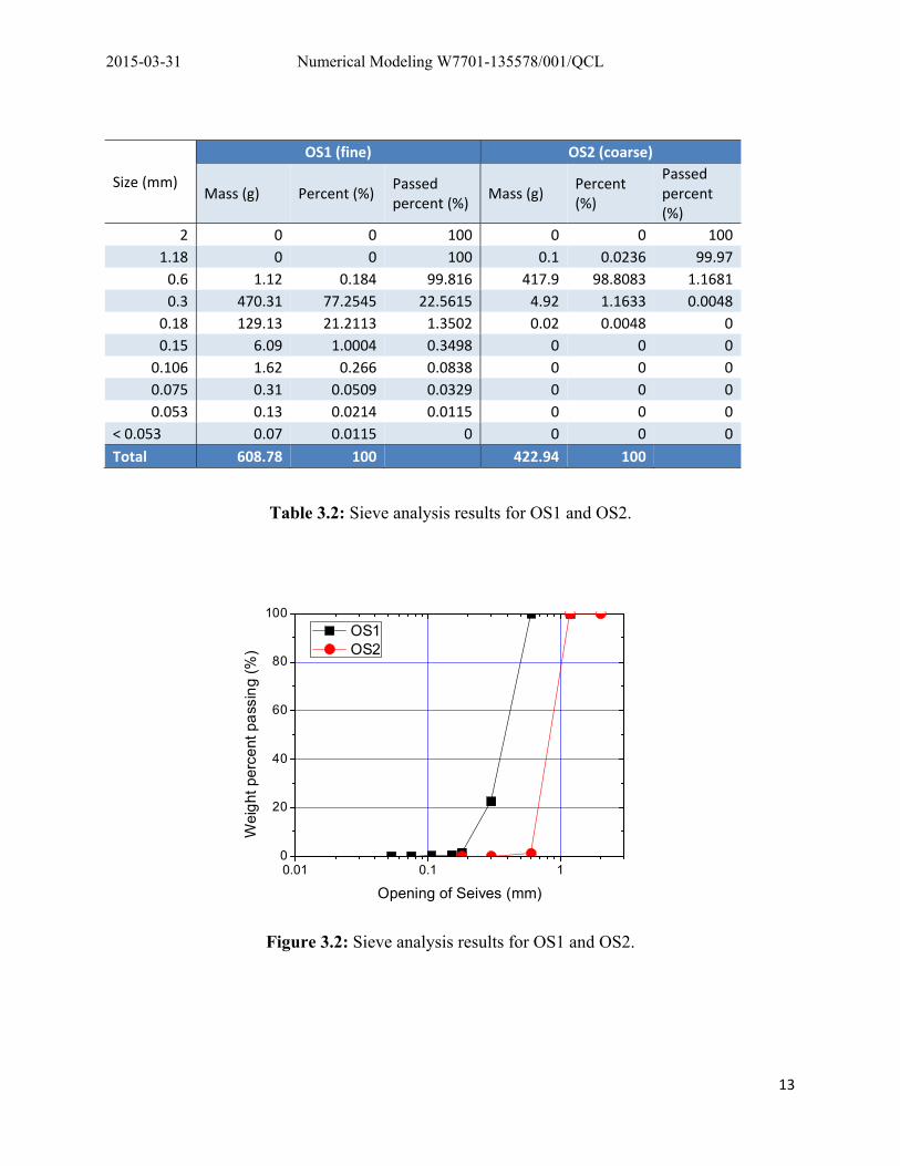
The sand used in the experiments was Ottawa sand (OS, shown in Figure 3.1). Both a fine grained (Figure 3.1 left) and coarse grained (Figure 3.1 right) sand were investigated over the course of the research program. The physical properties of each of these sands were measured and are reported in Table 3.1, and the particle size distributions for each sand is plotted in Figure 3.1 and summarized in Table 3.2.
Figure 3.1 Ottawa Sand: fine grained sand OS1 (left) and coarse grain sand OS2 (right).
Parameter Dimension OS1 (fine) OS2 (coarse)
Particle Density g/cm3 2.635 2.653
Bulk Density g/cm3 1.596 1.664
Void Ratio 0.651 2.653
Table 3.1: Physical properties of the sand used in the experiments
2015-03-31 Numerical Modeling W7701-135578/001/QCL
13
Size (mm)
OS1 (fine) OS2 (coarse)
Mass (g) Percent (%) Passed percent (%)
Mass (g) Percent (%)
Passed percent (%)
2 0 0 100 0 0 100
1.18 0 0 100 0.1 0.0236 99.97
0.6 1.12 0.184 99.816 417.9 98.8083 1.1681
0.3 470.31 77.2545 22.5615 4.92 1.1633 0.0048
0.18 129.13 21.2113 1.3502 0.02 0.0048 0
0.15 6.09 1.0004 0.3498 0 0 0
0.106 1.62 0.266 0.0838 0 0 0
0.075 0.31 0.0509 0.0329 0 0 0
0.053 0.13 0.0214 0.0115 0 0 0
< 0.053 0.07 0.0115 0 0 0 0
Total 608.78 100 422.94 100
Table 3.2: Sieve analysis results for OS1 and OS2.
0.01 0.1 10
20
40
60
80
100
Wei
ght p
erce
nt p
assi
ng (%
)
Opening of Seives (mm)
OS1 OS2
Figure 3.2: Sieve analysis results for OS1 and OS2.
2015-03-31 Numerical Modeling W7701-135578/001/QCL
14
3.3 Dynamic experimental results on dry sand
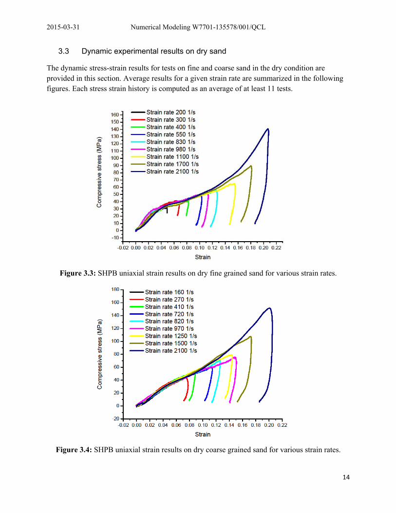
The dynamic stress-strain results for tests on fine and coarse sand in the dry condition are provided in this section. Average results for a given strain rate are summarized in the following figures. Each stress strain history is computed as an average of at least 11 tests.
Figure 3.3: SHPB uniaxial strain results on dry fine grained sand for various strain rates.
Figure 3.4: SHPB uniaxial strain results on dry coarse grained sand for various strain rates.
2015-03-31 Numerical Modeling W7701-135578/001/QCL
15
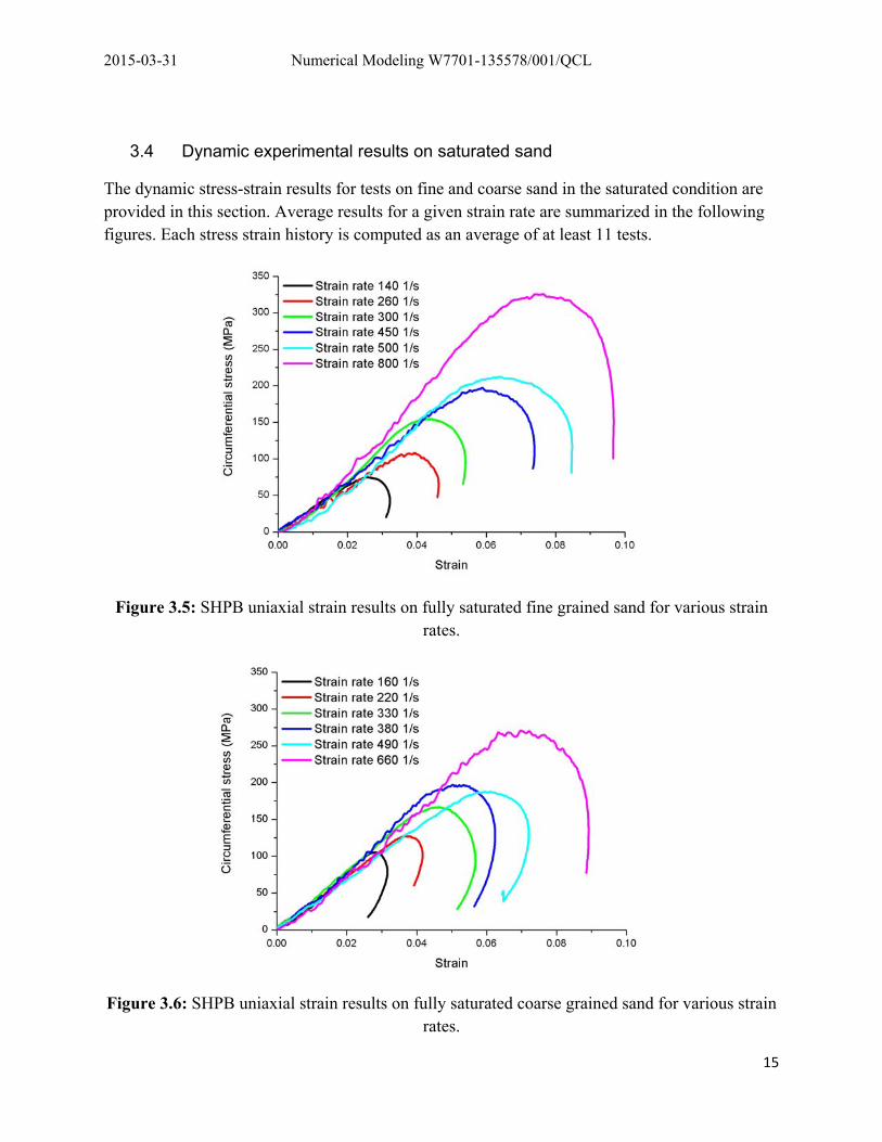
3.4 Dynamic experimental results on saturated sand
The dynamic stress-strain results for tests on fine and coarse sand in the saturated condition are provided in this section. Average results for a given strain rate are summarized in the following figures. Each stress strain history is computed as an average of at least 11 tests.
Figure 3.5: SHPB uniaxial strain results on fully saturated fine grained sand for various strain rates.
Figure 3.6: SHPB uniaxial strain results on fully saturated coarse grained sand for various strain rates.
2015-03-31 Numerical Modeling W7701-135578/001/QCL
16
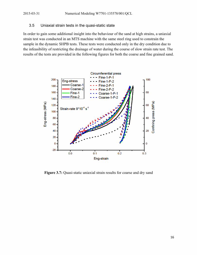
3.5 Uniaxial strain tests in the quasi-static state
In order to gain some additional insight into the behaviour of the sand at high strains, a uniaxial strain test was conducted in an MTS machine with the same steel ring used to constrain the sample in the dynamic SHPB tests. These tests were conducted only in the dry condition due to the infeasibility of restricting the drainage of water during the course of slow strain rate test. The results of the tests are provided in the following figures for both the coarse and fine grained sand.
Figure 3.7: Quasi-static uniaxial strain results for coarse and dry sand
2015-03-31 Numerical Modeling W7701-135578/001/QCL
17
Chapter 4: Calibration of the constitutive model
Constitutive model parametrisation follows from the experimental data by recasting the constitutive problem where stresses are determined as a function of strain increments, to one of nonlinear optimisation, where both the stress and strain trajectories are specified (i.e. the experiment) under unknown model parameters (i.e. the elastic parameters, the surface and cap parameters, and the viscosity parameters). For example, given the objective function, F:
min min ;
where P is a vector containing the undetermined parameters we wish to solve for by the minimisation of the function F; are the set of known strains; are the stresses
determined from the experiment; and are the stresses computed from the constitutive model. The constitutive model was recast in this form (in MATLAB) and the Marquardt-Levenberg optimisation algorithm was used to solve for the vector of unknown parameters P. This method is similar to that used by Simo et al. (1988), to fit cap parameters to their model.
It should be noted that this problem, even with the availability of extensive experimental data, is non-unique, and therefore several combinations of parameters may possibly result in a suitable parametrised constitutive model. For this reason, several parameters were fixed (at values typical for sand), and other values were determined through the optimisation procedure.
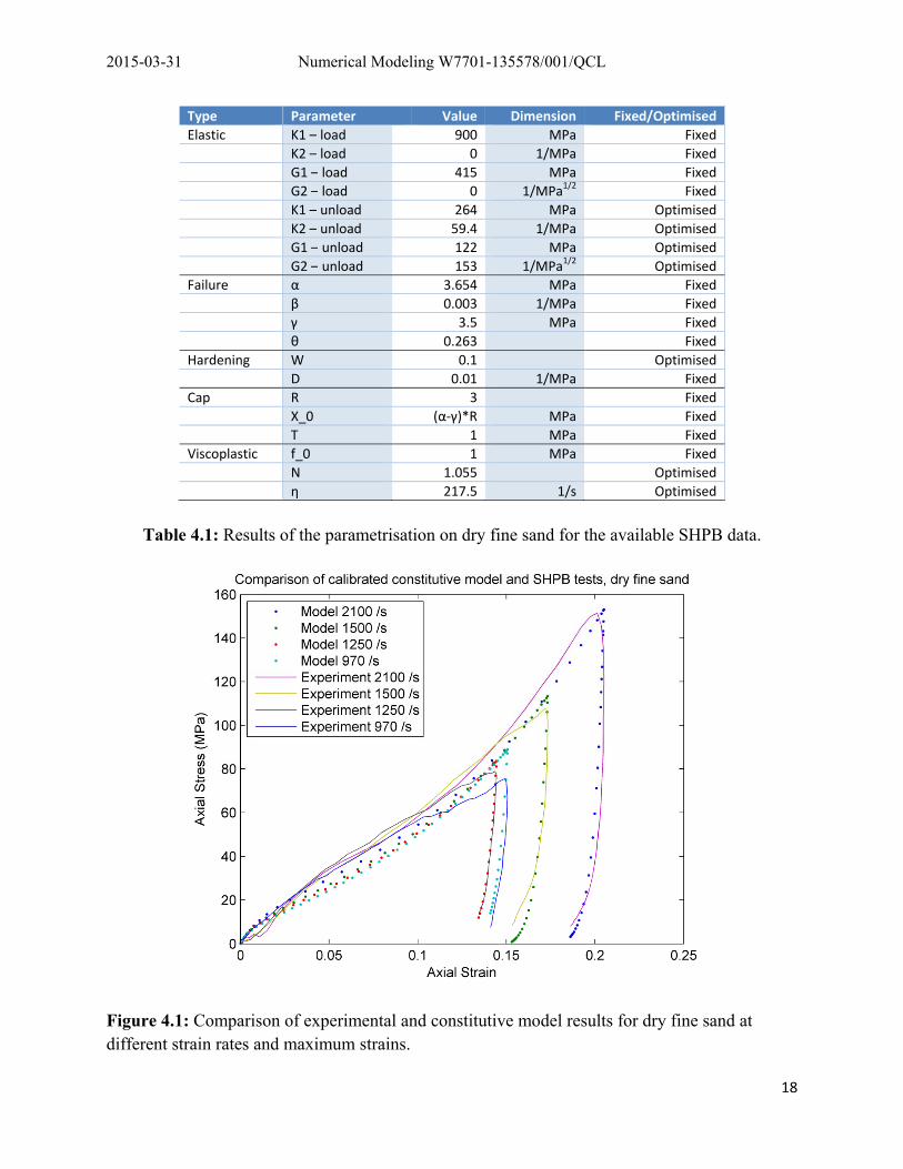
4.1 Calibration of fine grained dry sand
The results of the calibration for the fine grained dry sand are provided in Table 4.1. In this model, a nonlinear exponential unloading elastic stiffness tensor is used (with coefficient K1 and G1, and exponent K2 and G2). The loading elastic stiffness tensor is linear. Model output for several experimental tests is provided in Figure 4.1.
4.2 Calibration of coarse grained dry sand
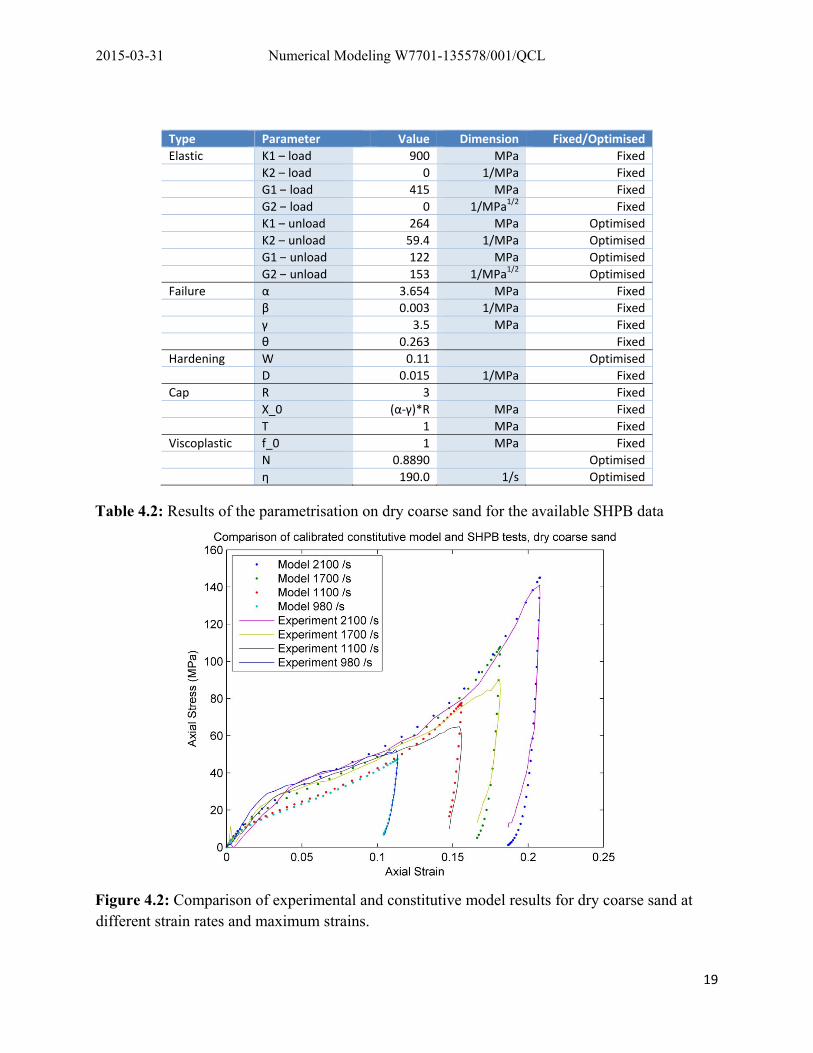
The results of the calibration for the coarse grained dry sand are provided in Table 4.2. In this model, a nonlinear exponential unloading elastic stiffness tensor is used (with coefficient K1 and G1, and exponents K2 and G2). The loading elastic stiffness tensor is linear. Model output for several experimental tests is provided in Figure 4.2.
2015-03-31 Numerical Modeling W7701-135578/001/QCL
18
Type Parameter Value Dimension Fixed/Optimised
Elastic K1 – load 900 MPa Fixed
K2 – load 0 1/MPa Fixed
G1 – load 415 MPa Fixed
G2 – load 0 1/MPa1/2 Fixed
K1 – unload 264 MPa Optimised
K2 – unload 59.4 1/MPa Optimised
G1 – unload 122 MPa Optimised
G2 – unload 153 1/MPa1/2 Optimised
Failure α 3.654 MPa Fixed
β 0.003 1/MPa Fixed
γ 3.5 MPa Fixed
θ 0.263 Fixed
Hardening W 0.1 Optimised
D 0.01 1/MPa Fixed
Cap R 3 Fixed
X_0 (α‐γ)*R MPa Fixed
T 1 MPa Fixed
Viscoplastic f_0 1 MPa Fixed
N 1.055 Optimised
η 217.5 1/s Optimised
Table 4.1: Results of the parametrisation on dry fine sand for the available SHPB data.
Figure 4.1: Comparison of experimental and constitutive model results for dry fine sand at different strain rates and maximum strains.
2015-03-31 Numerical Modeling W7701-135578/001/QCL
19
Type Parameter Value Dimension Fixed/Optimised
Elastic K1 – load 900 MPa Fixed
K2 – load 0 1/MPa Fixed
G1 – load 415 MPa Fixed
G2 – load 0 1/MPa1/2 Fixed
K1 – unload 264 MPa Optimised
K2 – unload 59.4 1/MPa Optimised
G1 – unload 122 MPa Optimised
G2 – unload 153 1/MPa1/2 Optimised
Failure α 3.654 MPa Fixed
β 0.003 1/MPa Fixed
γ 3.5 MPa Fixed
θ 0.263 Fixed
Hardening W 0.11 Optimised
D 0.015 1/MPa Fixed
Cap R 3 Fixed
X_0 (α‐γ)*R MPa Fixed
T 1 MPa Fixed
Viscoplastic f_0 1 MPa Fixed
N 0.8890 Optimised
η 190.0 1/s Optimised
Table 4.2: Results of the parametrisation on dry coarse sand for the available SHPB data
Figure 4.2: Comparison of experimental and constitutive model results for dry coarse sand at different strain rates and maximum strains.
2015-03-31 Numerical Modeling W7701-135578/001/QCL
20
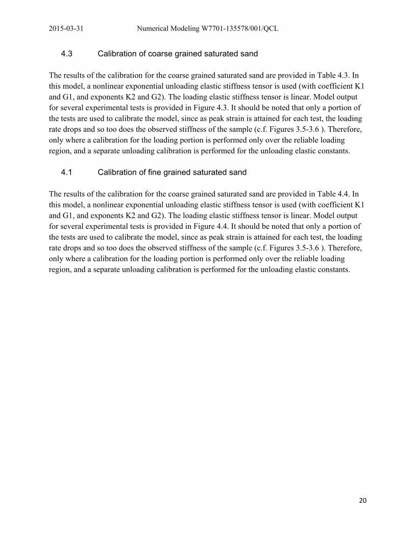
4.3 Calibration of coarse grained saturated sand The results of the calibration for the coarse grained saturated sand are provided in Table 4.3. In this model, a nonlinear exponential unloading elastic stiffness tensor is used (with coefficient K1 and G1, and exponents K2 and G2). The loading elastic stiffness tensor is linear. Model output for several experimental tests is provided in Figure 4.3. It should be noted that only a portion of the tests are used to calibrate the model, since as peak strain is attained for each test, the loading rate drops and so too does the observed stiffness of the sample (c.f. Figures 3.5-3.6 ). Therefore, only where a calibration for the loading portion is performed only over the reliable loading region, and a separate unloading calibration is performed for the unloading elastic constants.
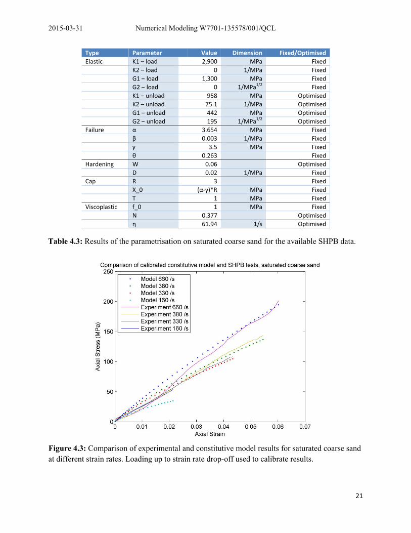
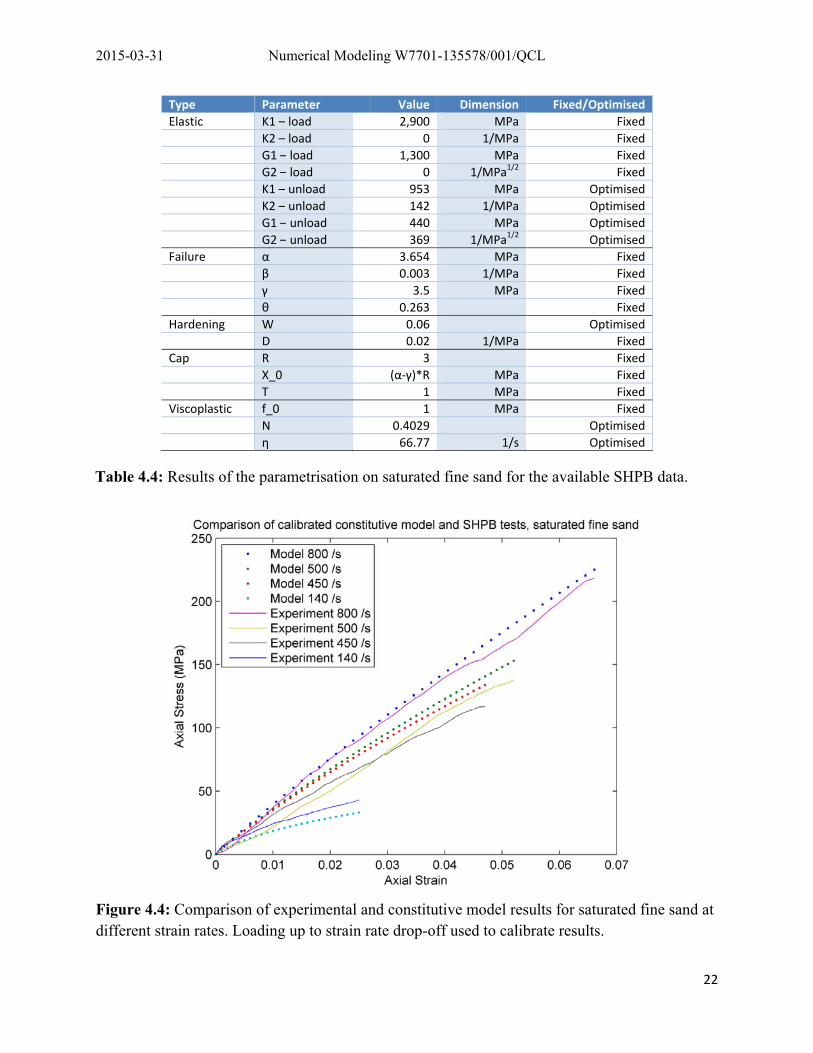
4.1 Calibration of fine grained saturated sand The results of the calibration for the coarse grained saturated sand are provided in Table 4.4. In this model, a nonlinear exponential unloading elastic stiffness tensor is used (with coefficient K1 and G1, and exponents K2 and G2). The loading elastic stiffness tensor is linear. Model output for several experimental tests is provided in Figure 4.4. It should be noted that only a portion of the tests are used to calibrate the model, since as peak strain is attained for each test, the loading rate drops and so too does the observed stiffness of the sample (c.f. Figures 3.5-3.6 ). Therefore, only where a calibration for the loading portion is performed only over the reliable loading region, and a separate unloading calibration is performed for the unloading elastic constants.
2015-03-31 Numerical Modeling W7701-135578/001/QCL
21
Type Parameter Value Dimension Fixed/Optimised
Elastic K1 – load 2,900 MPa Fixed
K2 – load 0 1/MPa Fixed
G1 – load 1,300 MPa Fixed
G2 – load 0 1/MPa1/2 Fixed
K1 – unload 958 MPa Optimised
K2 – unload 75.1 1/MPa Optimised
G1 – unload 442 MPa Optimised
G2 – unload 195 1/MPa1/2 Optimised
Failure α 3.654 MPa Fixed
β 0.003 1/MPa Fixed
γ 3.5 MPa Fixed
θ 0.263 Fixed
Hardening W 0.06 Optimised
D 0.02 1/MPa Fixed
Cap R 3 Fixed
X_0 (α‐γ)*R MPa Fixed
T 1 MPa Fixed
Viscoplastic f_0 1 MPa Fixed
N 0.377 Optimised
η 61.94 1/s Optimised
Table 4.3: Results of the parametrisation on saturated coarse sand for the available SHPB data.
Figure 4.3: Comparison of experimental and constitutive model results for saturated coarse sand at different strain rates. Loading up to strain rate drop-off used to calibrate results.
2015-03-31 Numerical Modeling W7701-135578/001/QCL
22
Type Parameter Value Dimension Fixed/Optimised
Elastic K1 – load 2,900 MPa Fixed
K2 – load 0 1/MPa Fixed
G1 – load 1,300 MPa Fixed
G2 – load 0 1/MPa1/2 Fixed
K1 – unload 953 MPa Optimised
K2 – unload 142 1/MPa Optimised
G1 – unload 440 MPa Optimised
G2 – unload 369 1/MPa1/2 Optimised
Failure α 3.654 MPa Fixed
β 0.003 1/MPa Fixed
γ 3.5 MPa Fixed
θ 0.263 Fixed
Hardening W 0.06 Optimised
D 0.02 1/MPa Fixed
Cap R 3 Fixed
X_0 (α‐γ)*R MPa Fixed
T 1 MPa Fixed
Viscoplastic f_0 1 MPa Fixed
N 0.4029 Optimised
η 66.77 1/s Optimised
Table 4.4: Results of the parametrisation on saturated fine sand for the available SHPB data.
Figure 4.4: Comparison of experimental and constitutive model results for saturated fine sand at different strain rates. Loading up to strain rate drop-off used to calibrate results.
2015-03-31 Numerical Modeling W7701-135578/001/QCL
23
Chapter 5: Equation of State
Accurate modelling of blast waves through solids requires the use of an equation of state (EOS) to predict the volumetric (hydrostatic) response of the material, especially when volumetric strains are extremely high. In some cases, the shear stresses of the material being modelled are neglected, since these are minimal in relation to the volumetrically induced pressures. Otherwise, a constitutive relation can be defined that models only the deviatoric portion of the stress-strain relation, whereas the hydrostatic portion is modelled through a suitable equation of state.
This chapter briefly outlines the theoretical framework of the three-phase EOS proposed by Wang et al. (2004) and developed by An et al. (2011) for a two or three phase material (such as unsaturated, partially saturated, or fully saturated sand). A numerical procedure for computing the material bulk modulus or pressure based on a change in the material volume (as is the case in an LS-DYNA hydrocode simulation) is presented. Finally, suitable parameters based on experiments conducted by Chapman et al. (2006) are presented. The FORTRAN source code for direct implementation into the LS-DYNA user defined subroutine files (dyn21b.F) is documented in Appendix C.
5.1 Three-Phase Equation of State
The three phase equation of state is an extension of the Mie-Gruneisen equation of state for modelling the pressure-volume-energy relations for media consisting of more than one phase. The known initial volume and mass ratios of each phase (silica sand, water, and air) are used to compute the relative pressure contribution to the total material pressure and specific energy for a given state.
The conservation of mass, momentum, and energy in a soil in a shocked state (subscript H), in comparison to the reference state (subscript o), can be expressed as follows:
2
where denotes the shock velocity and denotes the particle velocity, is the volume of the
material, and is the density. The Hugoniot of a material can be expressed as the relation between the shock velocity and the particle velocity as follows:
2015-03-31 Numerical Modeling W7701-135578/001/QCL
24
where is the sound speed at the reference pressure and temperature, and is the linear coefficient. From the conservation of mass and the Hugoniot relation above, we have:
1 ∆
where ∆ is the volumetric strain. Similarly,
∆∆
1 ∆.
Letting
1 1
We have
∆1
Substituting and into the conservation of momentum equation yields,
1 ∆∆
1 ∆∆
1 ∆
and finally, substituting the expression for yields,
1
1 1
.
A more accurate representation than the uniaxial strain case can be obtained by expressing the pressure in terms of the Gruneisen parameter :
2015-03-31 Numerical Modeling W7701-135578/001/QCL
25
where is the internal energy per unit mass for the Hugoniot (reference state), and is the energy per unit mass. From the conservation of energy, the above expression yields the Mie-Gruneisen equation:
12
If the Gruneisen parameter is expressed as follows
where is the first-order volume correction, we have
11
.
Substituting and into the Mie-Gruneisen equation yields
1 1 2 21
. 5.1
where / , the energy per unit initial volume. This equation can be used to compute the pressures of each of the three soil phases individually. The bulk modulus of the material is given as follows:
1 1 2 2 1 2 11 1 1 21
…1
. 5.2 .
The changes of volume fractions can be computed over the course of a pressure change in the material. Letting , , and be the initial volume fractions of the solid, water, and air phases respectively; ∗, ∗ , and ∗ the new volume fractions under the change in pressure; and , , and the initial densities, we have the following relations:
1
.
2015-03-31 Numerical Modeling W7701-135578/001/QCL
26
The changes in volume fraction can be computed as
∗ 1/
5.3
∗ 1/
5.3
∗/
. 5.3
where the , , and are the exponents of the specific entropy for the solid water and air phases respectively. The soil density under pressure is
∗ ∗ ∗ Denoting the weight fractions of the solid, water and air phases , , and respectively, we have
and,
.
5.2 Numerical Implementation of the Equation of State
In this section, the simple numerical procedure for implementing the three-phase equation of state is outlined in pseudocode. In LS-DYNA, the program passes the user defined EOS the change in volumetric strain (along with several history variables which include, among others, energy, volume fractions, previous volumetric changes for each phase), and the corresponding pressure, or bulk modulus is computed (depending on which is requested by the program). For the full source code, see Appendix C.
1. If first = true (first call of subroutine at integration node), initialize history variables
hist(1) = , , hist(2) = , , hist(3) = ,
hist(4) = 0.0 , hist(5) = 0.0 , hist(6) = 0.0

2015-03-31 Numerical Modeling W7701-135578/001/QCL
27
2. Compute weight ratios for each phase
, / , and similarly for water and air phases
3. Determine the specific energy for each phase
, and similarly for water and air phases
4. Compute the volume ratios (df / ) for each phase
df df ∙ / , and similarly for water and air phases
5. Compute for composite and each phase
1, 1,and similarly for water and air phases
6. Compute the original volumes of solid, air and water
, df ∙ 2 ∙ vol ∙ , and similarly for water and air phases
7. If iflag = 0, compute bulk modulus (Eq. 5.2), and return
8. If iflag = 1, compute the pressures of each phase using Eq. 5.1, and ensure all are above the cutoff pressure (pcut), continue
9. Compute the specific energy for each phase, and sum
0.5 ∙ ∙ vol / , ∙
….
10. If vol 0.0, compute new pressure by
∙ vol ∙ vol ∙ vol
vol
else,
11. Compute new volume ratios ( ∗ , ∗ , and ∗ ) by Equations 5.3a-c
2015-03-31 Numerical Modeling W7701-135578/001/QCL
28
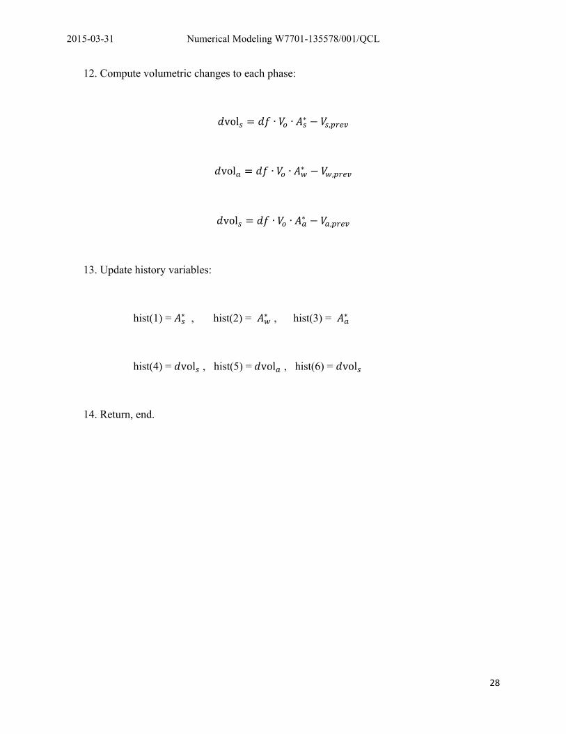
12. Compute volumetric changes to each phase:
vol ∙ ∙ ∗,
vol ∙ ∙ ∗,
vol ∙ ∙ ∗,
13. Update history variables:
hist(1) = ∗ , hist(2) = ∗ , hist(3) = ∗
hist(4) = vol , hist(5) = vol , hist(6) = vol
14. Return, end.
2015-03-31 Numerical Modeling W7701-135578/001/QCL
29
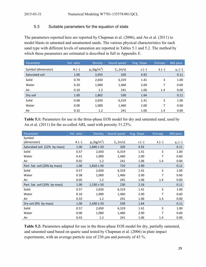
5.3 Suitable parameters for the equation of state
The parameters reported here are reported by Chapman et al. (2006), and An et al. (2011) to model blasts in saturated and unsaturated sands. The various physical characteristics for each sand type with different levels of saturation are reported in Tables 5.1 and 5.2. The method by which these parameters are estimated is described in full in Appendix E.
Parameter Vol. ratio Density Sound speed Hug. Slope Entropy MG para.
Symbol (dimension) A (‐‐) ρο (kg/m3) Co (m/s) s (‐‐) k (‐‐) γo (‐‐)
Saturated soil 1.00 2,055 320 4.92 0.11
Solid 0.70 2,650 6,319 1.41 3 1.00
Water 0.20 1,000 1,460 2.00 7 0.60
Air 0.10 1.2 241 1.06 1.4 0.00
Dry soil 1.00 1,802 530 1.64 0.11
Solid 0.68 2,650 6,319 1.41 3 1.00
Water 0.00 1,000 1,460 2.00 7 0.60
Air 0.32 1.2 241 1.06 1.4 0.00
Table 5.1: Parameters for use in the three-phase EOS model for dry and saturated sand, used by An et al. (2011) for the so-called ARL sand with porosity 31.23%.
Parameter Vol. ratio Density Sound speed Hug. Slope Entropy MG para.
Symbol (dimension) A (‐‐) ρο (kg/m
3) Co (m/s) s (‐‐) k (‐‐) γo (‐‐)
Saturated soil (22% by mass) 1.00 1,840 ± 50 320 4.92 0.11
Solid 0.57 2,650 6,319 1.41 3 1.00
Water 0.41 1,000 1,460 2.00 7 0.60
Air 0.02 1.2 241 1.06 1.4 0.00
Part. Sat. soil (20% by mass) 1.00 1,810 ± 50 710 2.90 0.11
Solid 0.57 2,650 6,319 1.41 3 1.00
Water 0.38 1,000 1,460 2.00 7 0.60
Air 0.05 1.2 241 1.06 1.4 0.00
Part. Sat. soil (10% by mass) 1.00 1,530 ± 50 230 2.26 0.11
Solid 0.57 2,650 6,319 1.41 3 1.00
Water 0.10 1,000 1,460 2.00 7 0.60
Air 0.33 1.2 241 1.06 1.4 0.00
Dry soil (0% by mass) 1.00 1,430 ± 50 530 1.64 0.11
Solid 0.57 2,650 6,319 1.41 3 1.00
Water 0.00 1,000 1,460 2.00 7 0.60
Air 0.43 1.2 241 1.06 1.4 0.00
Table 5.2: Parameters adapted for use in the three-phase EOS model for dry, partially saturated, and saturated sand based on quartz sand tested by Chapman et al. (2006) in plate impact experiments, with an average particle size of 230 μm and porosity of 43 %.
2015-03-31 Numerical Modeling W7701-135578/001/QCL
30
Chapter 6: Numerical simulation
In order to determine the validity and the performance of the subroutines developed as part of this research project, several preliminary numerical simulations were conducted and compared to results readily available in the open literature for similar materials. In this chapter, the subroutines for the constitutive model and EOS are run with parameters reported by An et al. (2011) and compared to experimental results reported in the same paper.
6.1 Model Geometry and Parameters
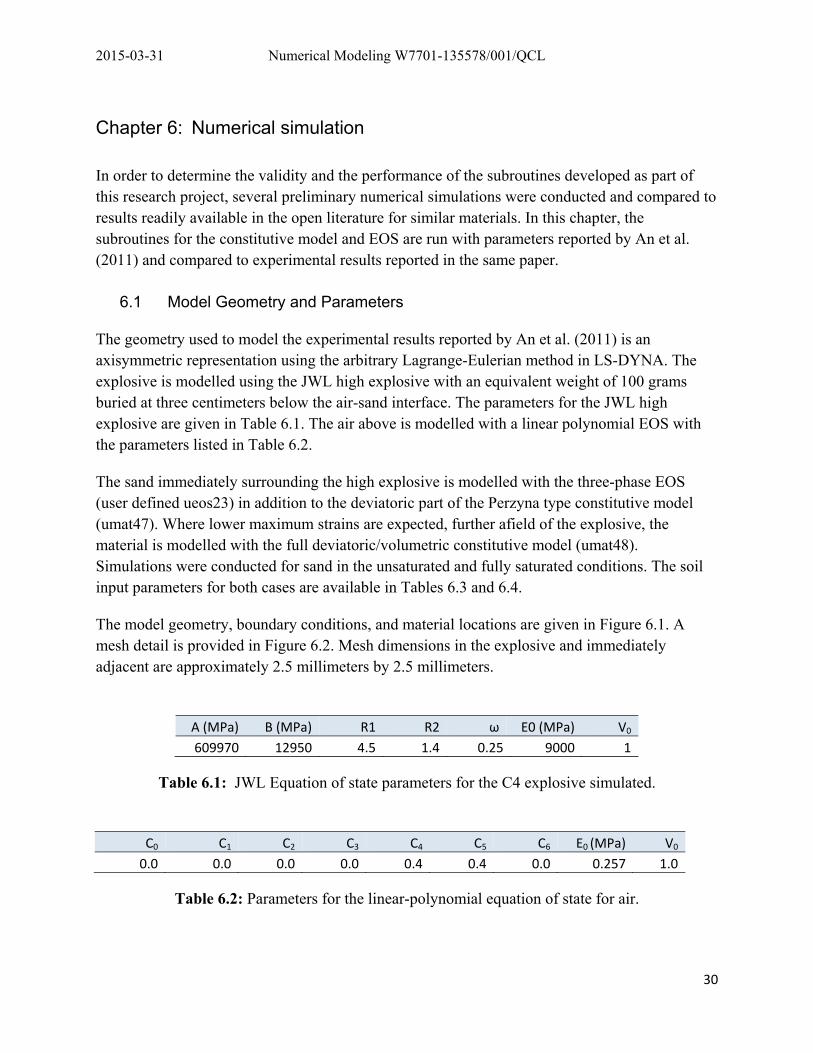
The geometry used to model the experimental results reported by An et al. (2011) is an axisymmetric representation using the arbitrary Lagrange-Eulerian method in LS-DYNA. The explosive is modelled using the JWL high explosive with an equivalent weight of 100 grams buried at three centimeters below the air-sand interface. The parameters for the JWL high explosive are given in Table 6.1. The air above is modelled with a linear polynomial EOS with the parameters listed in Table 6.2.
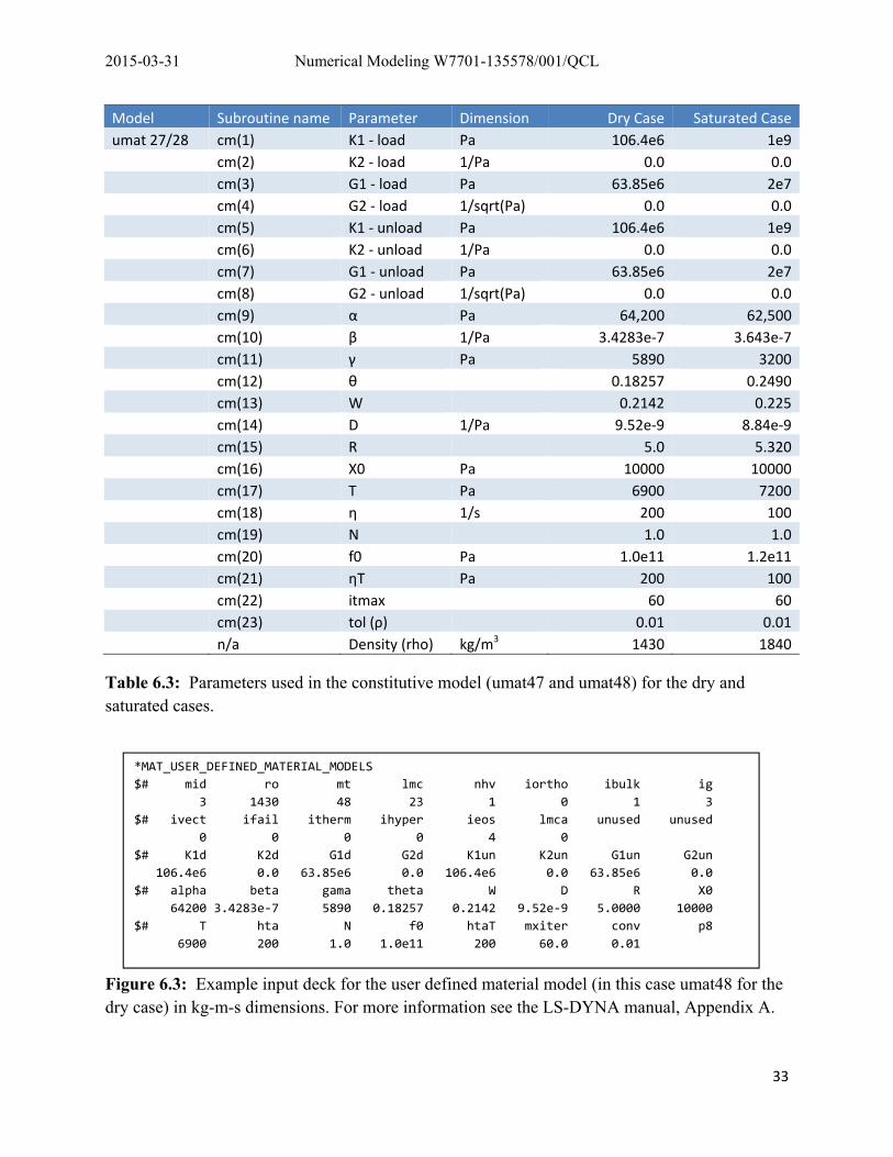
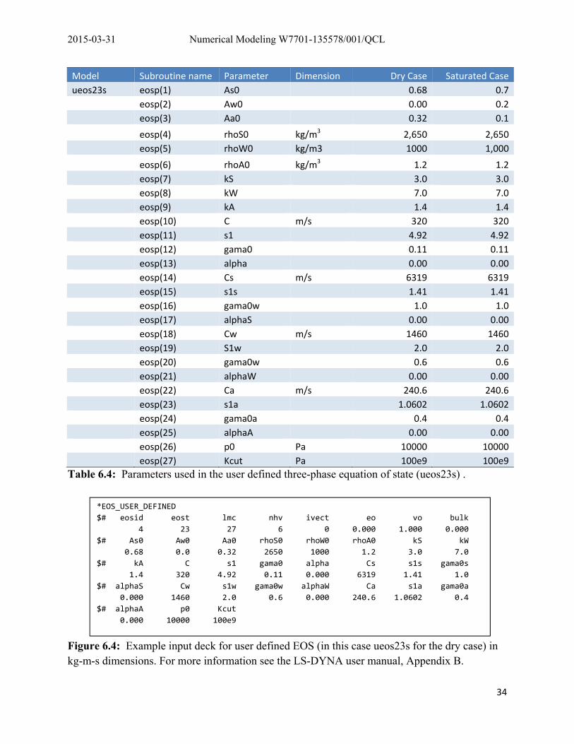
The sand immediately surrounding the high explosive is modelled with the three-phase EOS (user defined ueos23) in addition to the deviatoric part of the Perzyna type constitutive model (umat47). Where lower maximum strains are expected, further afield of the explosive, the material is modelled with the full deviatoric/volumetric constitutive model (umat48). Simulations were conducted for sand in the unsaturated and fully saturated conditions. The soil input parameters for both cases are available in Tables 6.3 and 6.4.
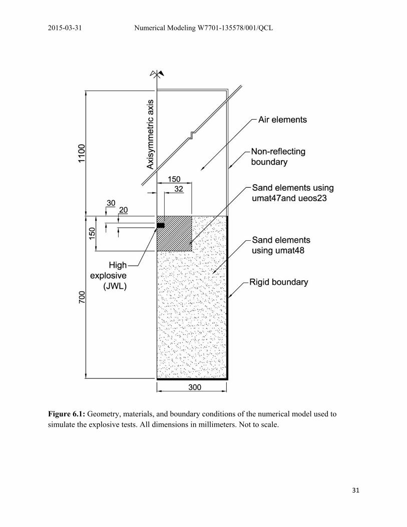
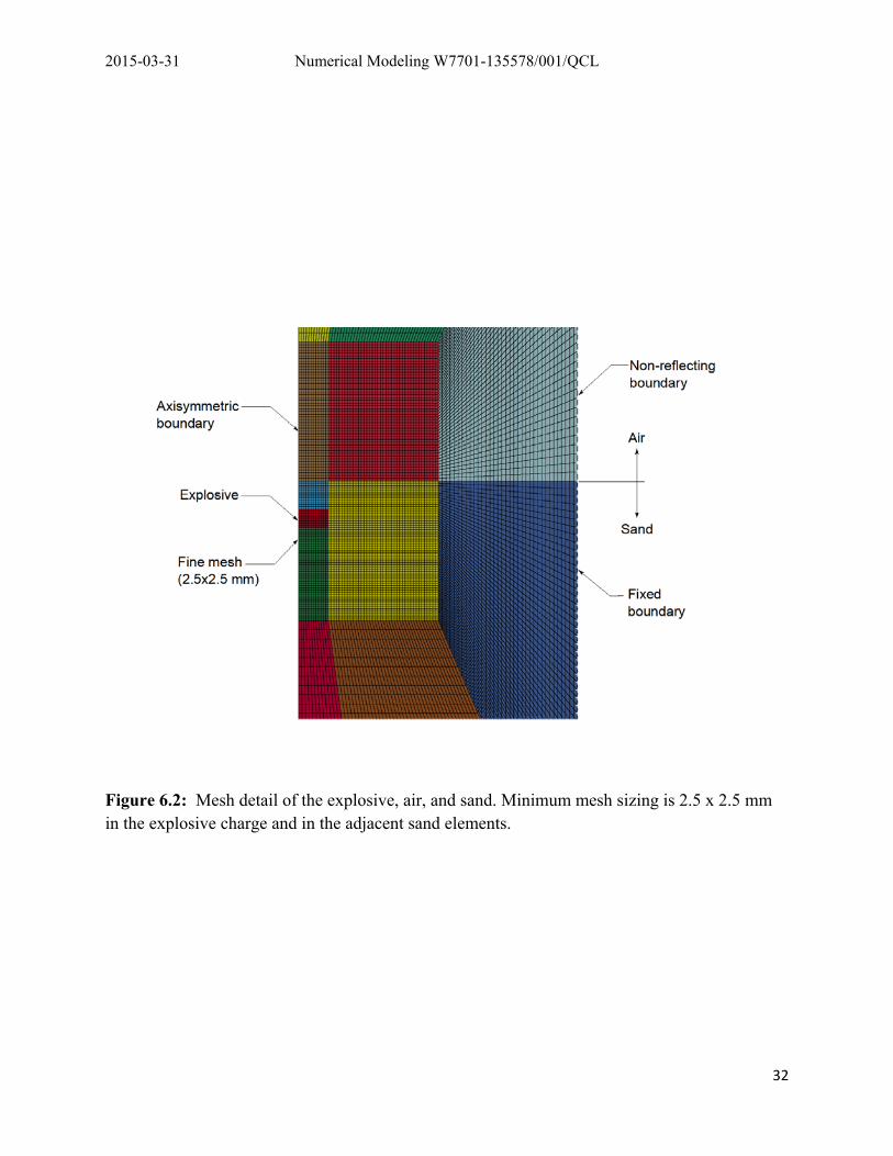
The model geometry, boundary conditions, and material locations are given in Figure 6.1. A mesh detail is provided in Figure 6.2. Mesh dimensions in the explosive and immediately adjacent are approximately 2.5 millimeters by 2.5 millimeters.
A (MPa) B (MPa) R1 R2 ω E0 (MPa) V0
609970 12950 4.5 1.4 0.25 9000 1
Table 6.1: JWL Equation of state parameters for the C4 explosive simulated.
C0 C1 C2 C3 C4 C5 C6 E0 (MPa) V0
0.0 0.0 0.0 0.0 0.4 0.4 0.0 0.257 1.0
Table 6.2: Parameters for the linear-polynomial equation of state for air.
2015-03-31 Numerical Modeling W7701-135578/001/QCL
31
Figure 6.1: Geometry, materials, and boundary conditions of the numerical model used to simulate the explosive tests. All dimensions in millimeters. Not to scale.
2015-03-31 Numerical Modeling W7701-135578/001/QCL
32
Figure 6.2: Mesh detail of the explosive, air, and sand. Minimum mesh sizing is 2.5 x 2.5 mm in the explosive charge and in the adjacent sand elements.
2015-03-31 Numerical Modeling W7701-135578/001/QCL
33
Model Subroutine name Parameter Dimension Dry Case Saturated Case
umat 27/28 cm(1) K1 ‐ load Pa 106.4e6 1e9
cm(2) K2 ‐ load 1/Pa 0.0 0.0
cm(3) G1 ‐ load Pa 63.85e6 2e7
cm(4) G2 ‐ load 1/sqrt(Pa) 0.0 0.0
cm(5) K1 ‐ unload Pa 106.4e6 1e9
cm(6) K2 ‐ unload 1/Pa 0.0 0.0
cm(7) G1 ‐ unload Pa 63.85e6 2e7
cm(8) G2 ‐ unload 1/sqrt(Pa) 0.0 0.0
cm(9) α Pa 64,200 62,500
cm(10) β 1/Pa 3.4283e‐7 3.643e‐7
cm(11) γ Pa 5890 3200
cm(12) θ 0.18257 0.2490
cm(13) W 0.2142 0.225
cm(14) D 1/Pa 9.52e‐9 8.84e‐9
cm(15) R 5.0 5.320
cm(16) X0 Pa 10000 10000
cm(17) T Pa 6900 7200
cm(18) η 1/s 200 100
cm(19) N 1.0 1.0
cm(20) f0 Pa 1.0e11 1.2e11
cm(21) ηT Pa 200 100
cm(22) itmax 60 60
cm(23) tol (ρ) 0.01 0.01
n/a Density (rho) kg/m3 1430 1840
Table 6.3: Parameters used in the constitutive model (umat47 and umat48) for the dry and saturated cases. Figure 6.3: Example input deck for the user defined material model (in this case umat48 for the dry case) in kg-m-s dimensions. For more information see the LS-DYNA manual, Appendix A.
*MAT_USER_DEFINED_MATERIAL_MODELS
$# mid ro mt lmc nhv iortho ibulk ig
3 1430 48 23 1 0 1 3
$# ivect ifail itherm ihyper ieos lmca unused unused
0 0 0 0 4 0
$# K1d K2d G1d G2d K1un K2un G1un G2un
106.4e6 0.0 63.85e6 0.0 106.4e6 0.0 63.85e6 0.0
$# alpha beta gama theta W D R X0
64200 3.4283e‐7 5890 0.18257 0.2142 9.52e‐9 5.0000 10000
$# T hta N f0 htaT mxiter conv p8
6900 200 1.0 1.0e11 200 60.0 0.01
2015-03-31 Numerical Modeling W7701-135578/001/QCL
34
Model Subroutine name Parameter Dimension Dry Case Saturated Case
ueos23s eosp(1) As0 0.68 0.7
eosp(2) Aw0 0.00 0.2
eosp(3) Aa0 0.32 0.1
eosp(4) rhoS0 kg/m3 2,650 2,650
eosp(5) rhoW0 kg/m3 1000 1,000
eosp(6) rhoA0 kg/m3 1.2 1.2
eosp(7) kS 3.0 3.0
eosp(8) kW 7.0 7.0
eosp(9) kA 1.4 1.4
eosp(10) C m/s 320 320
eosp(11) s1 4.92 4.92
eosp(12) gama0 0.11 0.11
eosp(13) alpha 0.00 0.00
eosp(14) Cs m/s 6319 6319
eosp(15) s1s 1.41 1.41
eosp(16) gama0w 1.0 1.0
eosp(17) alphaS 0.00 0.00
eosp(18) Cw m/s 1460 1460
eosp(19) S1w 2.0 2.0
eosp(20) gama0w 0.6 0.6
eosp(21) alphaW 0.00 0.00
eosp(22) Ca m/s 240.6 240.6
eosp(23) s1a 1.0602 1.0602
eosp(24) gama0a 0.4 0.4
eosp(25) alphaA 0.00 0.00
eosp(26) p0 Pa 10000 10000
eosp(27) Kcut Pa 100e9 100e9
Table 6.4: Parameters used in the user defined three-phase equation of state (ueos23s) .
Figure 6.4: Example input deck for user defined EOS (in this case ueos23s for the dry case) in kg-m-s dimensions. For more information see the LS-DYNA user manual, Appendix B.
*EOS_USER_DEFINED
$# eosid eost lmc nhv ivect eo vo bulk
4 23 27 6 0 0.000 1.000 0.000
$# As0 Aw0 Aa0 rhoS0 rhoW0 rhoA0 kS kW
0.68 0.0 0.32 2650 1000 1.2 3.0 7.0
$# kA C s1 gama0 alpha Cs s1s gama0s
1.4 320 4.92 0.11 0.000 6319 1.41 1.0
$# alphaS Cw s1w gama0w alphaW Ca s1a gama0a
0.000 1460 2.0 0.6 0.000 240.6 1.0602 0.4
$# alphaA p0 Kcut
0.000 10000 100e9
2015-03-31 Numerical Modeling W7701-135578/001/QCL
35
6.2 Model results
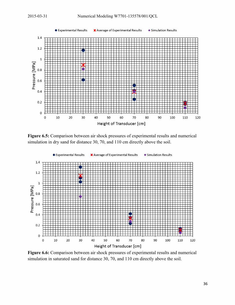
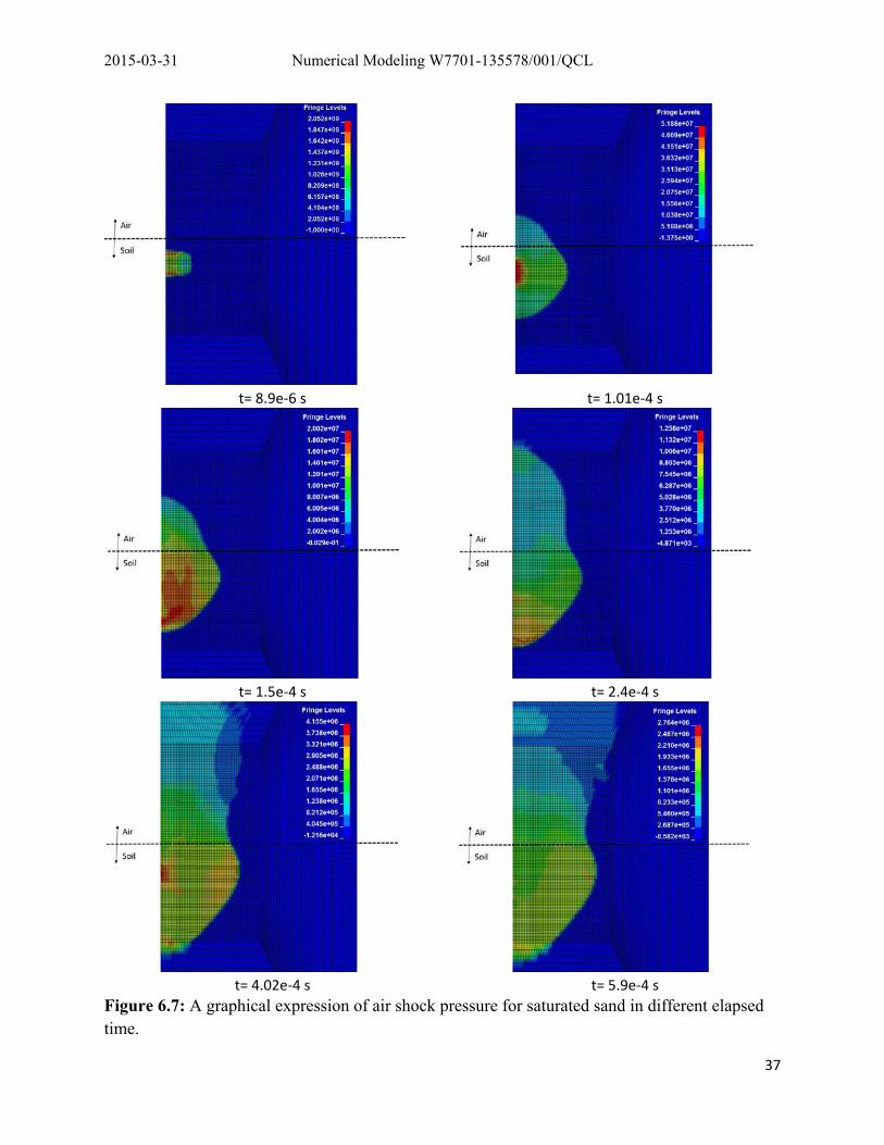
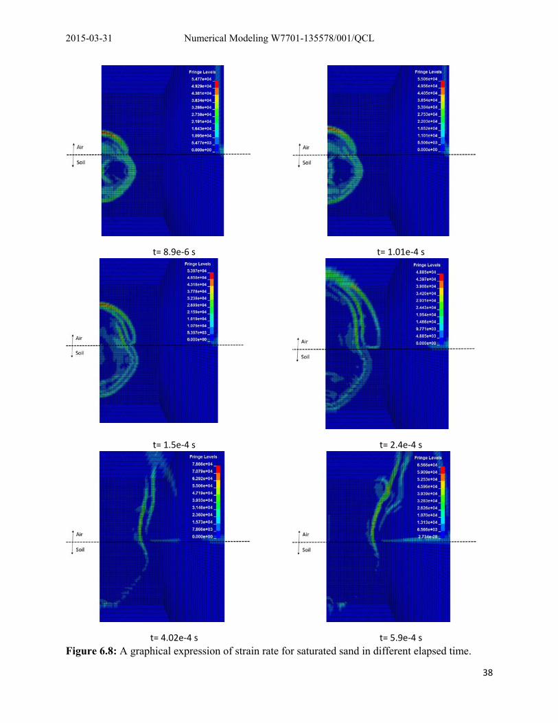
As stated in the previous section, to evaluate the credibility of the subroutines in LS-DYNA, the explosion test results presented in the An et al. (2011) have been used. In general, six explosion tests have been reported: three for the dry sand; and three for the saturated sand. Figure 6.5 and 6.6 show the air shock pressures predicted by numerical simulation (pink square), the experimental results (dark blue circle), and average values of the experimental results (red star) at the distances of the 30, 70, 110 cm above the soil (the heights of the transducers). The difference between the averages of experimental results and predicated values shows that the predicted results have a quite good agreement with the experimental results (except for the results for saturated sand at 30 cm distance). In addition, graphical expressions of the distribution of the air shock pressure and strain rate near the explosive material (C4) are shown in Figures 6.7 and 6.8. Based on the simulation results, the maximum strain rate in soil has been around 2.0 10 s-1 and occurred at the beginning of the explosion in the sand near of the explosive material. By moving the wave in the sand, the strain rate decreases as is expected.
2015-03-31 Numerical Modeling W7701-135578/001/QCL
36
Figure 6.5: Comparison between air shock pressures of experimental results and numerical simulation in dry sand for distance 30, 70, and 110 cm directly above the soil.
Figure 6.6: Comparison between air shock pressures of experimental results and numerical simulation in saturated sand for distance 30, 70, and 110 cm directly above the soil.
2015-03-31 Numerical Modeling W7701-135578/001/QCL
37
t= 8.9e‐6 s t= 1.01e‐4 s
t= 1.5e‐4 s t= 2.4e‐4 s
t= 4.02e‐4 s t= 5.9e‐4 s
Figure 6.7: A graphical expression of air shock pressure for saturated sand in different elapsed time.
2015-03-31 Numerical Modeling W7701-135578/001/QCL
38
t= 8.9e‐6 s t= 1.01e‐4 s
t= 1.5e‐4 s t= 2.4e‐4 s
t= 4.02e‐4 s t= 5.9e‐4 s
Figure 6.8: A graphical expression of strain rate for saturated sand in different elapsed time.
2015-03-31 Numerical Modeling W7701-135578/001/QCL
39
Conclusion
In this report, a comprehensive investigation into the dynamic constitutive behaviour of sand has been presented. Beginning with data from dynamic tests (both Split Hopkinson Pressure Bar tests and Plate Impact experiments), an understanding of the rate dependent material behaviour was derived. Building on the developments of other researchers, a Perzyna-type viscoplastic model and a three-phase equation of state were implemented numerically. The non-unique Perzyna viscoplastic model was calibrated using a Marquardt-Levenberg optimisation algorithm, and the EOS parameters were derived from known properties of sand and its constituent phases. Finally, the validity of the numerical models was tested against explosion tests available from the literature.
In addition to a comprehensive description of the constitutive behaviour of sand over several orders of magnitude of strain rate, this report can be used as framework for the future study of other types of soils such as clay, silt, and gravel.
2015-03-31 Numerical Modeling W7701-135578/001/QCL
40
References
An, J., Tuan, C.Y., Cheeseman, B.A., Gazonas, G.A., Simulation of Soil Behavior under Blast Loading, International Journal of Geomechanics, 11:323-334, 2011.
An, J. Soil Behavior under Blast Loading, Ph.D. dissertation, University of Nebraska - Lincoln
Chapman, D.J., Tsembelis, K., Proud, W.G., The Behaviour of Water Saturated Sand under Shock-loading, Proc. SEM Annual Conference and Exposition on Experimental and Applied Mechanics, St. Louis, 400-406, 2006.
Chen, W., Saleeb A.F., Constitutive Equations for Engineering Materials, Vol.1-2, Elsevier, 1994.
Grujicic, M., He, T., Pandurangan, B., Bell, W.C., Cheeseman, B.A., Roy, W.N., Skaggs, R.R., Development, parametrisation, and validation of a visco-plastic material model for sand with different levels of water saturation, Proc. IMechE Vol. 223 Part L: J. Materials: Design and Application, 2009.
Katona, M.G., Evaluation of Viscoplastic Cap Model, Journal of Geotechnical Engineering, 110:1106-1125, 1984.
Omidvar, M., Iskander, M., Bless, S., Stress-strain behavior of sand at high strain rates, International Journal of Impact Engineering, 49:192-213, 2012.
Perzyna, P., Fundamental Problems in Viscolplasticity, Advances in Applied Mechanics, Vol. 9, 243-377, 1966.
Simo, J.C., Ju, J., Pister, K.S., Taylor R.L., Assessment of Cap Model: Consistent Return Algorithms and Rate-Dependent Extension, Journal of Engineering Mechanics, 114:191-218, 1988.
Tong, S., Tuan, C.Y., Viscoplastic Cap Model for Soils under High Strain Rate Loading, Journal of Geotechnical and Geoenvironmental Engineering, 133:206-204, 2007.
Wang, W.M. Stationary and Propagative Instabilities in Metals – A Computational Point of View, Ph.D. dissertation, TU Delft, 1997.
Wang, Z. Hao, H., Lu, Y., A three-phase soil model for simulating stress wave propagation due to blast loading, International Journal for Numerical and Analytical Methods in Geomechanics, 28:33-56, 2004.
2015-03-31 Numerical Modeling W7701-135578/001/QCL
41
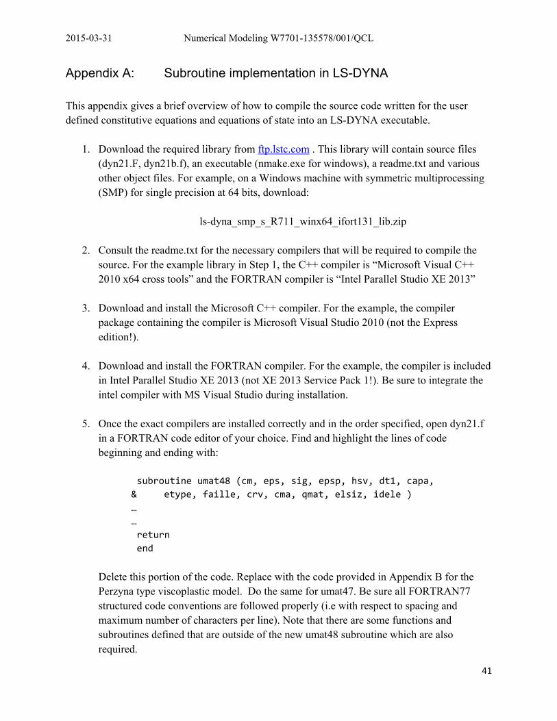
Appendix A: Subroutine implementation in LS-DYNA This appendix gives a brief overview of how to compile the source code written for the user defined constitutive equations and equations of state into an LS-DYNA executable.
1. Download the required library from ftp.lstc.com . This library will contain source files (dyn21.F, dyn21b.f), an executable (nmake.exe for windows), a readme.txt and various other object files. For example, on a Windows machine with symmetric multiprocessing (SMP) for single precision at 64 bits, download: ls-dyna_smp_s_R711_winx64_ifort131_lib.zip
2. Consult the readme.txt for the necessary compilers that will be required to compile the source. For the example library in Step 1, the C++ compiler is “Microsoft Visual C++ 2010 x64 cross tools” and the FORTRAN compiler is “Intel Parallel Studio XE 2013”
3. Download and install the Microsoft C++ compiler. For the example, the compiler package containing the compiler is Microsoft Visual Studio 2010 (not the Express edition!).
4. Download and install the FORTRAN compiler. For the example, the compiler is included in Intel Parallel Studio XE 2013 (not XE 2013 Service Pack 1!). Be sure to integrate the intel compiler with MS Visual Studio during installation.
5. Once the exact compilers are installed correctly and in the order specified, open dyn21.f in a FORTRAN code editor of your choice. Find and highlight the lines of code beginning and ending with: subroutine umat48 (cm, eps, sig, epsp, hsv, dt1, capa, & etype, faille, crv, cma, qmat, elsiz, idele )
…
…
return
end
Delete this portion of the code. Replace with the code provided in Appendix B for the Perzyna type viscoplastic model. Do the same for umat47. Be sure all FORTRAN77 structured code conventions are followed properly (i.e with respect to spacing and maximum number of characters per line). Note that there are some functions and subroutines defined that are outside of the new umat48 subroutine which are also required.
2015-03-31 Numerical Modeling W7701-135578/001/QCL
42
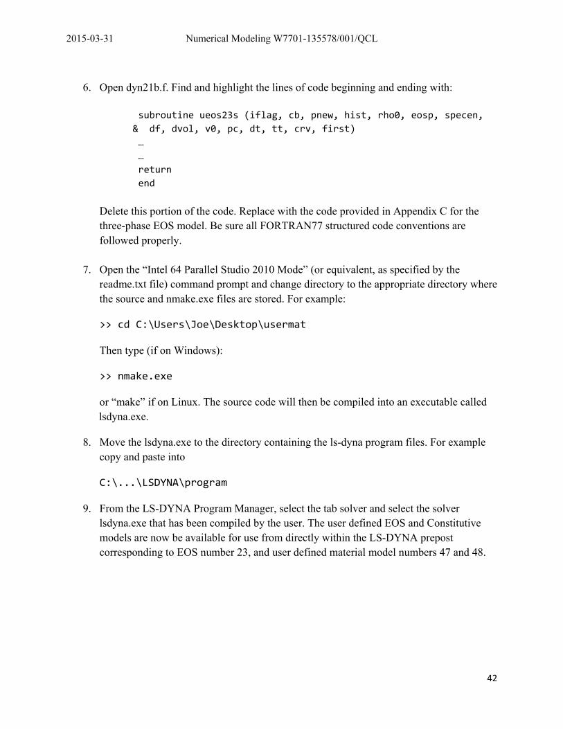
6. Open dyn21b.f. Find and highlight the lines of code beginning and ending with:
subroutine ueos23s (iflag, cb, pnew, hist, rho0, eosp, specen,
& df, dvol, v0, pc, dt, tt, crv, first)
…
…
return
end
Delete this portion of the code. Replace with the code provided in Appendix C for the three-phase EOS model. Be sure all FORTRAN77 structured code conventions are followed properly.
7. Open the “Intel 64 Parallel Studio 2010 Mode” (or equivalent, as specified by the readme.txt file) command prompt and change directory to the appropriate directory where the source and nmake.exe files are stored. For example:
>> cd C:\Users\Joe\Desktop\usermat
Then type (if on Windows):
>> nmake.exe
or “make” if on Linux. The source code will then be compiled into an executable called lsdyna.exe.
8. Move the lsdyna.exe to the directory containing the ls-dyna program files. For example copy and paste into
C:\...\LSDYNA\program
9. From the LS-DYNA Program Manager, select the tab solver and select the solver lsdyna.exe that has been compiled by the user. The user defined EOS and Constitutive models are now be available for use from directly within the LS-DYNA prepost corresponding to EOS number 23, and user defined material model numbers 47 and 48.
2015-03-31 Numerical Modeling W7701-135578/001/QCL
43
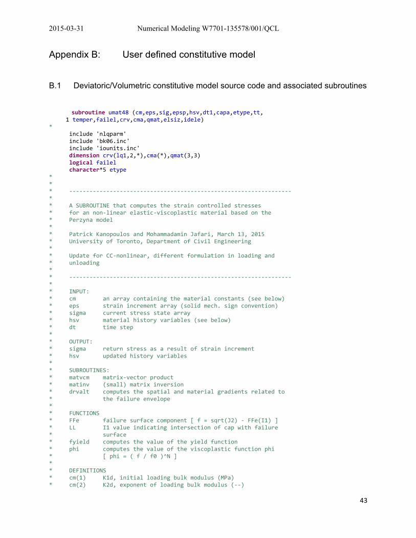
Appendix B: User defined constitutive model
B.1 Deviatoric/Volumetric constitutive model source code and associated subroutines
subroutine umat48 (cm,eps,sig,epsp,hsv,dt1,capa,etype,tt, 1 temper,failel,crv,cma,qmat,elsiz,idele) * include 'nlqparm' include 'bk06.inc' include 'iounits.inc' dimension crv(lq1,2,*),cma(*),qmat(3,3) logical failel character*5 etype * * * ‐‐‐‐‐‐‐‐‐‐‐‐‐‐‐‐‐‐‐‐‐‐‐‐‐‐‐‐‐‐‐‐‐‐‐‐‐‐‐‐‐‐‐‐‐‐‐‐‐‐‐‐‐‐‐‐‐‐‐‐‐‐‐‐‐‐ * * A SUBROUTINE that computes the strain controlled stresses * for an non‐linear elastic‐viscoplastic material based on the * Perzyna model * * Patrick Kanopoulos and Mohammadamin Jafari, March 13, 2015 * University of Toronto, Department of Civil Engineering * * Update for CC‐nonlinear, different formulation in loading and * unloading * * ‐‐‐‐‐‐‐‐‐‐‐‐‐‐‐‐‐‐‐‐‐‐‐‐‐‐‐‐‐‐‐‐‐‐‐‐‐‐‐‐‐‐‐‐‐‐‐‐‐‐‐‐‐‐‐‐‐‐‐‐‐‐‐‐‐‐ * * INPUT: * cm an array containing the material constants (see below) * eps strain increment array (solid mech. sign convention) * sigma current stress state array * hsv material history variables (see below) * dt time step * * OUTPUT: * sigma return stress as a result of strain increment * hsv updated history variables * * SUBROUTINES: * matvcm matrix‐vector product * matinv (small) matrix inversion * drvalt computes the spatial and material gradients related to * the failure envelope * * FUNCTIONS * FFe failure surface component [ f = sqrt(J2) ‐ FFe(I1) ] * LL I1 value indicating intersection of cap with failure * surface * fyield computes the value of the yield function * phi computes the value of the viscoplastic function phi * [ phi = ( f / f0 )^N ] * * DEFINITIONS * cm(1) K1d, initial loading bulk modulus (MPa) * cm(2) K2d, exponent of loading bulk modulus (‐‐)
2015-03-31 Numerical Modeling W7701-135578/001/QCL
44
* cm(3) G1d, initial loading shear modulus (GPa) * cm(4) G2d, exponent of loading shear modulus (‐‐) * cm(5) K1un, initial unloading bulk modulus (MPa) * cm(6) K2un, exponent of unloading bulk modulus (‐‐) * cm(7) G1un, initial unloading shear modulus (GPa) * cm(8) G2un, exponent of unloading shear modulus (‐‐) * cm(9) alpha, failure surface parameter (MPa) * cm(10) beta, failure surface parameter (MPa) * cm(11) gama, failure surface parameter (MPa) * cm(12) theta, failure surface parameter (‐‐) * cm(13) W, cap suface parameter (‐‐) * cm(14) D, cap surface parameter (‐‐) * cm(15) R, cap surface parameter (‐‐) * cm(16) X0, volumetric viscoplastic strain hardening const. (‐‐) * cm(17) T, tension cutoff (MPa) * cm(18) hta, viscoplastic fluidity parameter (inverse sec.) * cm(19) N, visplastic exponent * cm(20) f0, viscoplastic denomenator * cm(21) htaT, tensile vp fluidity parameter (inv. sec.) * cm(22) maximum number of iterations (convert to INTEGER) * cm(23) return mappaing tolerance (‐‐) * * hsv(1) kappa, hardeing parameter (‐‐) * * ‐‐‐‐‐‐‐‐‐‐‐‐‐‐‐‐‐‐‐‐‐‐‐‐‐‐‐‐‐‐‐‐‐‐‐‐‐‐‐‐‐‐‐‐‐‐‐‐‐‐‐‐‐‐‐‐‐‐‐‐‐‐‐‐‐‐ * * Initialize variable names and dimensions * * ‐‐‐‐‐‐‐‐‐‐‐‐‐‐‐‐‐‐‐‐‐‐‐‐‐‐‐‐‐‐‐‐‐‐‐‐‐‐‐‐‐‐‐‐‐‐‐‐‐‐‐‐‐‐‐‐‐‐‐‐‐‐‐‐‐‐ * implicit none * IO real cm(23), eps(6), sig(6), hsv(1), dt1 * * Stresses real sigma(6,1), sigtri(6,1), & dsigtr(6,1), sstri(6,1), I1tri, J2tri, prstri, signew(6,1), & I1new, J2new, ssnew(6,1), rj2tri, prsnew, Jratio * * Strains real deps(6,1), depsv, epsvp, epsvp0, depsvp * * parameters real K1d, K2d, G1d, G2d, K1un, K2un, G1un, G2un, alpha, beta, & gama, theta, W, D, R, T, hta, N, lame, f0, & CC(6,6), CCsup(6,6), CCinv(6,6), X0, htaT * real K1, K2, G1, G2 * * hardening parameters real kappa0, kappaN, dkappa, Xitr * * time domain parameters real dt * * Domain geometry variables real LLk, FFeTT, ftri integer domain integer vpyield * * return mapping variables real lamdaN, rhoN,
2015-03-31 Numerical Modeling W7701-135578/001/QCL
45
& conv, HH(6,6), HHinv(6,6), xi, xi1(6,1), & xi2(6,1), xi3(1,1), xi4, xxPL(6,1), yyPL(6,1) * * derivatives real dfs(6,1), ddfss(6,6), ddfsl(6,1), dphis(6,1), dphil, dkl, & tdphis(1,6) * * function calls real LL, FFe, fyield, phi, XX * * counting variables and iteration variables integer i, ii, mxiter * * other variables real phiN, lamoht *‐‐‐‐‐‐‐‐‐‐‐‐‐‐‐‐‐‐‐‐‐‐‐‐‐‐‐‐‐‐‐‐‐‐‐‐‐‐‐‐‐‐‐‐‐‐‐‐‐‐‐‐‐‐‐‐‐‐‐‐‐‐‐‐‐‐‐‐‐‐ * * VARIABLE ASSIGNMENT * *‐‐‐‐‐‐‐‐‐‐‐‐‐‐‐‐‐‐‐‐‐‐‐‐‐‐‐‐‐‐‐‐‐‐‐‐‐‐‐‐‐‐‐‐‐‐‐‐‐‐‐‐‐‐‐‐‐‐‐‐‐‐‐‐‐‐‐‐‐‐ * assign the stresses, sigma // convert to g.mech convention sigma(1,1) = ‐sig(6) sigma(2,1) = ‐sig(6) sigma(3,1) = ‐sig(6) sigma(4,1) = ‐sig(6) sigma(5,1) = ‐sig(6) sigma(6,1) = ‐sig(6) * * assign the strain increment, deps // convert to g.mech convention deps(1,1) = ‐eps(1) deps(2,1) = ‐eps(2) deps(3,1) = ‐eps(3) deps(4,1) = ‐eps(4) deps(5,1) = ‐eps(5) deps(6,1) = ‐eps(6) * * Assign elastic constants K1d = cm(1) K2d = cm(2) G1d = cm(3) G2d = cm(4) K1un = cm(5) K2un = cm(6) G1un = cm(7) G2un = cm(8) * * assign plastic constants alpha = cm(9) beta = cm(10) gama = cm(11) theta = cm(12) W = cm(13) D = cm(14) R = cm(15) X0 = cm(16) T = cm(17) * * assign viscocity constants hta = cm(18) N = cm(19) f0 = cm(20)
2015-03-31 Numerical Modeling W7701-135578/001/QCL
46
htaT = cm(21) * * Set default maximum iteration values mxiter = int(cm(22)) * * Set the convergence criterion conv = cm(23) * * assign initial value of hardening parameter kappa0 = hsv(1) kappaN = kappa0 * * assign timestep dt = dt1 * *‐‐‐‐‐‐‐‐‐‐‐‐‐‐‐‐‐‐‐‐‐‐‐‐‐‐‐‐‐‐‐‐‐‐‐‐‐‐‐‐‐‐‐‐‐‐‐‐‐‐‐‐‐‐‐‐‐‐‐‐‐‐‐‐‐‐‐‐‐‐ * * MAIN PROGRAM * *‐‐‐‐‐‐‐‐‐‐‐‐‐‐‐‐‐‐‐‐‐‐‐‐‐‐‐‐‐‐‐‐‐‐‐‐‐‐‐‐‐‐‐‐‐‐‐‐‐‐‐‐‐‐‐‐‐‐‐‐‐‐‐‐‐‐‐‐‐‐ * set elastic constants based on loading or unloading depsv = deps(1,1) + deps(2,1) + deps(3,1) if (depsv .GE. 0.0) then K1 = K1d K2 = K2d G1 = G1d G2 = G2d else K1 = K1un K2 = K2un G1 = G1un G2 = G2un endif * assemble the elastic stiffness tensor CC = 0 call CCnlin( CC, sigma, deps, K1, K2, G1, G2 ) CCsup = CC * compute the inverse stiffness tensor CCinv calling matinv call matinv(CCsup,6,CCinv) * * compute the elastic estimator stress, sigma^est_i * dsigtr = CC * depsilon call matvcm(6,6,CC,deps,dsigtr) sigtri = sigma + dsigtr * determine I1trial I1tri = sigtri(1,1)+sigtri(2,1)+sigtri(3,1) * determine J2trial (from pressure and sstrial) prstri = I1tri/3.0 sstri = sigtri sstri(1,1) = sigtri(1,1) ‐ prstri sstri(2,1) = sigtri(2,1) ‐ prstri sstri(3,1) = sigtri(3,1) ‐ prstri J2tri = 0.5*(sstri(1,1)**2 + sstri(2,1)**2 + sstri(3,1)**2) + & sstri(4,1)**2 + sstri(5,1)**2 + sstri(6,1)**2 * * ‐‐‐‐‐‐‐‐‐‐‐‐‐‐‐‐‐‐‐‐‐‐‐‐‐‐‐‐‐‐‐‐‐‐‐‐‐‐‐‐‐‐‐‐‐‐‐‐‐‐‐‐‐‐‐‐‐‐‐‐‐‐‐‐‐‐ * * Determine case (i.e. Tension lower quadrant, Tension higher * quadrant, Yield, Cap) * * Tension: domain 1 I1trial <= ‐T, and, root(J2trial) < FFe(‐T)
2015-03-31 Numerical Modeling W7701-135578/001/QCL
47
* Tension: domain 2 I1trial <= ‐T, and, root(J2trial) >= FFe(‐T) * Yield: domain 3 ‐T <= I1trial <= L(k) * Cap: domain 4 I1trial > L(k) * * ‐‐‐‐‐‐‐‐‐‐‐‐‐‐‐‐‐‐‐‐‐‐‐‐‐‐‐‐‐‐‐‐‐‐‐‐‐‐‐‐‐‐‐‐‐‐‐‐‐‐‐‐‐‐‐‐‐‐‐‐‐‐‐‐‐‐ LLk = LL(kappa0) FFeTT = FFe(T,alpha,gama,beta,theta) rJ2tri = sqrt(J2tri) if (I1tri .GT. LLk) then domain = 4 elseif ((I1tri .LE. LLk) .AND. (I1tri.GT.‐T)) then domain = 3 elseif ((I1tri.LE.‐T) .AND. (rJ2tri.GE.FFeTT)) then domain = 2 elseif ((I1tri.LE.‐T) .AND. (rJ2tri.LT.FFeTT)) then domain = 1 endif * Compute the value of fyield ftri = fyield(I1tri, J2tri, kappa0, domain, alpha, beta, gama, & theta, R, T) * Set logical yield variable (vpyield) to 1 or 0 if (ftri .GT. 0.) then vpyield = 1 else vpyield = 0 endif * * * ‐‐‐‐‐‐‐‐‐‐‐‐‐‐‐‐‐‐‐‐‐‐‐‐‐‐‐‐‐‐‐‐‐‐‐‐‐‐‐‐‐‐‐‐‐‐‐‐‐‐‐‐‐‐‐‐‐‐‐‐‐‐‐‐‐‐ * * MAIN if STATEMENT ‐‐ ELASTIC, RET. MAPPING, OR TENSION C.O. * * ‐‐‐‐‐‐‐‐‐‐‐‐‐‐‐‐‐‐‐‐‐‐‐‐‐‐‐‐‐‐‐‐‐‐‐‐‐‐‐‐‐‐‐‐‐‐‐‐‐‐‐‐‐‐‐‐‐‐‐‐‐‐‐‐‐‐ * If elastic step ‐ return elastic estimator * If viscoplastic step ‐ do return mapping * If tension step ‐ return tension cutoff stresses * ‐‐‐‐‐‐‐‐‐‐‐‐‐‐‐‐‐‐‐‐‐‐‐‐‐‐‐‐‐‐‐‐‐‐‐‐‐‐‐‐‐‐‐‐‐‐‐‐‐‐‐‐‐‐‐‐‐‐‐‐‐‐‐‐‐‐ if ((domain .EQ. 4 .OR. domain .EQ.3) .AND. vpyield .EQ. 0) then * output stress is simply the elastic trial stress, * hardening parameter (kappa) remains unchanged. signew = sigtri kappaN = kappa0 * * ‐‐‐‐‐‐‐‐‐‐‐‐‐‐‐‐‐‐‐‐‐‐‐‐‐‐‐‐‐‐‐‐‐‐‐‐‐‐‐‐‐‐‐‐‐‐‐‐‐‐‐‐‐‐‐‐‐‐‐‐‐‐‐‐‐‐ elseif ((domain .EQ. 4 .OR. domain .EQ. 3) & .AND. vpyield .EQ. 1) then * viscoplastic step! Do return mapping algorithm * * initialize initial variables (lamda, sigma, rho) lamdaN = 0.0 signew = sigtri rhoN = phi(signew,kappa0,domain,N,f0,alpha,beta,gama,theta,R,T) & ‐ lamdaN / (hta*dt) * compute initial volumetric vp strain, and initialize total and * incramental strains epsvp0 = W * (1 ‐ exp(‐D*
2015-03-31 Numerical Modeling W7701-135578/001/QCL
48
& ( XX(kappa0,R,alpha,gama,beta,theta)‐X0))) depsvp = 0.0 epsvp = 0.0 * * loop through iterative improvements of signew and kappa do 100 ii = 1,mxiter * find stress invariants for current stress state I1new = signew(1,1) + signew(2,1) + signew(3,1) prsnew = I1new/3.0 ssnew = signew ssnew(1,1) = signew(1,1) ‐ prsnew ssnew(2,1) = signew(2,1) ‐ prsnew ssnew(3,1) = signew(3,1) ‐ prsnew J2new = 0.5*(ssnew(1,1)**2 + ssnew(2,1)**2 + ssnew(3,1)**2) + & signew(4,1)**2 + signew(5,1)**2 + signew(6,1)**2 * compute stiffness tensor call CCnlin( CC, signew, deps, K1, K2, G1, G2 ) CCsup = CC call matinv(CCsup,6,CCinv) * call derivative subroutine ‐‐ returns necessary derivatives of * cap, failure, and phi functions call drvalt(I1new,J2new,ssnew,kappaN,domain,alpha,beta, & gama,theta, W, D, R, X0, N, f0, dfs, ddfss, ddfsl, & dphis, dphil, dkl, lamdaN ) * compute the HH vector // calling function minv (matrix inverse) HHinv = CCinv + lamdaN * ddfss * invert HHinv matrix to find HH, calling matinv call matinv(HHinv,6,HH) * take the transpose of dphis do 235 i=1,6 Tdphis(1,i)=dphis(i,1) 235 continue * compute xi calling the matrix‐vector multiplication subroutine * xi = Tdphis * HH * (dfs+lamdaN*ddfsl) + 1/(hta*dt) ‐ dphi xi1 = dfs + lamdaN*ddfsl call matvcm(6,6,HH,xi1,xi2) call matvcm(1,6,Tdphis,xi2,xi3) xi4 = xi3(1,1) xi = xi4 + ( 1.0 / (hta*dt) ) ‐ dphil * compute lamdaN lamdaN = lamdaN + rhoN/xi * compute {signew} = {signew} + [CC]*{depsilon ‐ lamdaN*dfs} xxPL = deps ‐ lamdaN * dfs call matvcm(6, 6, CC, xxPL, yyPL) signew = sigma + yyPL * Compute kappaN from dkappa = delta_lamda_N * dkappa/dlamda depsvp = lamdaN*( dfs(1,1) + dfs(2,1) + dfs(3,1) ) if (depsvp .LT. 0.0) depsvp = 0.0 epsvp = epsvp0 + depsvp if ( epsvp .GE. (0.99*W) ) then epsvp = 0.99*W signew = sigtri kappaN = kappa0 goto 300 endif Xitr = X0 ‐ log( 1 ‐ epsvp/W ) / D call ksolve(kappaN, Xitr, R, alpha, beta, gama, theta) * Check the convergence by computing rho_N
2015-03-31 Numerical Modeling W7701-135578/001/QCL
49
phiN = phi(signew,kappaN,domain,N,f0,alpha,beta,gama,theta,R,T) * compute rho for current iteration lamoht = lamdaN / (hta*dt) rhoN = phiN ‐ lamoht * Check for the convergence condition if ( abs(rhoN) .LE. abs(conv) ) then goto 300 endif * end loop 100 continue if (abs(rhoN) .gt. abs(conv)) then write(*,*) 'Not Converged, ii = ' , ii, 'rho_N = ', rhoN endif * * ‐‐‐‐‐‐‐‐‐‐‐‐‐‐‐‐‐‐‐‐‐‐‐‐‐‐‐‐‐‐‐‐‐‐‐‐‐‐‐‐‐‐‐‐‐‐‐‐‐‐‐‐‐‐‐‐‐‐‐‐‐‐‐‐‐‐ elseif (domain .EQ. 2 .OR. domain .EQ. 1 ) then * Tension cutoff stresses obtained ‐ return tensile stresses from * the tension formulas if (domain .EQ. 1) then * compute I1_new, pressure_new, J2_new, and 'Jratio' for domain 1 I1new = exp(‐htaT*dt)*I1tri + (1‐exp(‐htaT*dt))*(‐T) prsnew = I1new/3.0 J2new = J2tri Jratio = 1.0 else * compute I1_new, pressure_new, J2_new, and 'Jratio' for domain 2 I1new = exp(‐htaT*dt)*I1tri + (1‐exp(‐htaT*dt))*(‐T) prsnew = ‐I1new/3.0 J2new = ( exp(‐htaT*dt)*sqrt(J2tri) + (1‐exp(‐htaT*dt))* & FFeTT )**2 Jratio = sqrt(J2new)/sqrt(J2tri) endif * Update the stresses for the new tensile regime signew(1,1) = sstri(1,1)*Jratio + prsnew signew(2,1) = sstri(2,1)*Jratio + prsnew signew(3,1) = sstri(3,1)*Jratio + prsnew signew(4,1) = sstri(4,1)*Jratio signew(5,1) = sstri(5,1)*Jratio signew(6,1) = sstri(6,1)*Jratio endif 300 continue * * ‐‐‐‐‐‐‐‐‐‐‐‐‐‐‐‐‐‐‐‐‐‐‐‐‐‐‐‐‐‐‐‐‐‐‐‐‐‐‐‐‐‐‐‐‐‐‐‐‐‐‐‐‐‐‐‐‐‐‐‐‐‐‐‐‐‐ * * STRESS OUTPUT * * ‐‐‐‐‐‐‐‐‐‐‐‐‐‐‐‐‐‐‐‐‐‐‐‐‐‐‐‐‐‐‐‐‐‐‐‐‐‐‐‐‐‐‐‐‐‐‐‐‐‐‐‐‐‐‐‐‐‐‐‐‐‐‐‐‐‐ * update output variables sig // convert to solid mech. convention sig(1) = ‐signew(1,1) sig(2) = ‐signew(2,1) sig(3) = ‐signew(3,1) sig(4) = ‐signew(4,1) sig(5) = ‐signew(5,1) sig(6) = ‐signew(6,1) * update history variables
2015-03-31 Numerical Modeling W7701-135578/001/QCL
50
hsv = kappaN * return end * * ‐‐‐‐‐‐‐‐‐‐‐‐‐‐‐‐‐‐‐‐‐‐‐‐‐‐‐‐‐‐‐‐‐‐‐‐‐‐‐‐‐‐‐‐‐‐‐‐‐‐‐‐‐‐‐‐‐‐‐‐‐‐‐‐‐‐ * * FUNCTION DEFINITIONS * * ‐‐‐‐‐‐‐‐‐‐‐‐‐‐‐‐‐‐‐‐‐‐‐‐‐‐‐‐‐‐‐‐‐‐‐‐‐‐‐‐‐‐‐‐‐‐‐‐‐‐‐‐‐‐‐‐‐‐‐‐‐‐‐‐‐‐ * * ‐‐‐‐‐‐‐‐‐‐‐‐‐‐‐‐‐‐‐‐‐‐‐‐‐‐‐‐‐‐‐‐‐‐‐‐‐‐‐‐‐‐‐‐‐‐‐‐‐‐‐‐‐‐‐‐‐‐‐‐‐‐‐‐‐‐ * A FUNCTION that computes the value of the function F_e(I_1) which * is part of the yield surface function real function FFe (I1,alpha,gama,beta,theta) real I1,alpha,gama,beta,theta FFe = alpha ‐ gama*exp(‐beta*I1) + theta*I1 return end * ‐‐‐‐‐‐‐‐‐‐‐‐‐‐‐‐‐‐‐‐‐‐‐‐‐‐‐‐‐‐‐‐‐‐‐‐‐‐‐‐‐‐‐‐‐‐‐‐‐‐‐‐‐‐‐‐‐‐‐‐‐‐‐‐‐ * A FUNCTION that computes L(kappa) real function LL (kappa) real kappa if (kappa .GT. 0.0) then LL = kappa else LL = 0.0 endif return end * ‐‐‐‐‐‐‐‐‐‐‐‐‐‐‐‐‐‐‐‐‐‐‐‐‐‐‐‐‐‐‐‐‐‐‐‐‐‐‐‐‐‐‐‐‐‐‐‐‐‐‐‐‐‐‐‐‐‐‐‐‐‐‐‐‐‐ * A FUNCTION that computes X(k), i.e. intersection of the cap with * the I1‐axis real function XX (kappa,R,alpha,gama,beta,theta) real kappa,R,alpha,gama,beta,theta,FFe XX = kappa + R*FFe(kappa,alpha,gama,beta,theta) return end * ‐‐‐‐‐‐‐‐‐‐‐‐‐‐‐‐‐‐‐‐‐‐‐‐‐‐‐‐‐‐‐‐‐‐‐‐‐‐‐‐‐‐‐‐‐‐‐‐‐‐‐‐‐‐‐‐‐‐‐‐‐‐‐‐‐‐ * A FUNCTION that computes the value of the yield function f_yield real function fyield(I1, J2, kappa, domain, alpha, beta, gama, & theta, R, T) real I1, J2, kappa, alpha, gama, beta, theta, R, T, FFe real XX, LL, XXk, LLk integer domain if (domain .EQ. 4) then * cap surface LLk = LL(kappa) XXk = XX(kappa,R,alpha,gama,beta,theta) fyield = sqrt( (I1 ‐ LLk)**2.0 / R**2.0 + J2 ) + (LLk ‐ XXk)/R elseif (domain .EQ. 3) then * failure surface fyield = sqrt(J2) ‐ FFe(I1,alpha,gama,beta,theta) else fyield = I1 ‐ T
2015-03-31 Numerical Modeling W7701-135578/001/QCL
51
endif return end * ‐‐‐‐‐‐‐‐‐‐‐‐‐‐‐‐‐‐‐‐‐‐‐‐‐‐‐‐‐‐‐‐‐‐‐‐‐‐‐‐‐‐‐‐‐‐‐‐‐‐‐‐‐‐‐‐‐‐‐‐‐‐‐‐‐‐ * A FUNCTION to compute the value phi(sigma,kappa) real function phi(sigma, kappa, domain, N, f0, alpha, beta, gama, & theta, R, T) real sigma(6,1), ss(3,1), kappa, N, f0, alpha, gama, beta, R, prs, & f, fyield, I1, J2 integer domain * compute I2 and J2 I1 = sigma(1,1) + sigma(2,1) + sigma(3,1) prs = I1/3.0 ss(1,1) = sigma(1,1) ‐ prs ss(2,1) = sigma(2,1) ‐ prs ss(3,1) = sigma(3,1) ‐ prs J2 = 0.5*(ss(1,1)**2 + ss(2,1)**2 + ss(3,1)**2) & + sigma(4,1)**2 + sigma(5,1)**2 + sigma(6,1)**2 * Pass I2 and J2 to fyield to determine the value of f f = fyield(I1,J2,kappa,domain,alpha,beta,gama,theta,R,T) * ensure the value of f does not fall below 0 if (f .LT. 0.0) f = 0.0 * compute the value of phi phi = (f/f0)**N return end * * * ‐‐‐‐‐‐‐‐‐‐‐‐‐‐‐‐‐‐‐‐‐‐‐‐‐‐‐‐‐‐‐‐‐‐‐‐‐‐‐‐‐‐‐‐‐‐‐‐‐‐‐‐‐‐‐‐‐‐‐‐‐‐‐‐‐‐ * * SUBROUTINE SECTION * * ‐‐‐‐‐‐‐‐‐‐‐‐‐‐‐‐‐‐‐‐‐‐‐‐‐‐‐‐‐‐‐‐‐‐‐‐‐‐‐‐‐‐‐‐‐‐‐‐‐‐‐‐‐‐‐‐‐‐‐‐‐‐‐‐‐‐ * * subroutine drvalt(I1,J2,ss,kappa,domain,alpha,beta,gama, & theta, W, D, R, X0, N, f0, dfs, ddfss, ddfsl, & dphis, dphil, dkl, lamda) * ‐‐‐‐‐‐‐‐‐‐‐‐‐‐‐‐‐‐‐‐‐‐‐‐‐‐‐‐‐‐‐‐‐‐‐‐‐‐‐‐‐‐‐‐‐‐‐‐‐‐‐‐‐‐‐‐‐‐‐‐‐‐‐‐‐‐ * * A SUBROUTINE that computes the necessary derivatives for the * return mapping algorithm. * * INCLUDES ALTERNATE DEFINITION OF dkappa/klamda AND USES * LAMDA AS AN ADDITIONAL INPUT (FINAL ARGUMENT ABOVE) * * ‐‐‐‐‐‐‐‐‐‐‐‐‐‐‐‐‐‐‐‐‐‐‐‐‐‐‐‐‐‐‐‐‐‐‐‐‐‐‐‐‐‐‐‐‐‐‐‐‐‐‐‐‐‐‐‐‐‐‐‐‐‐‐‐‐‐ * * INPUT: * I1new first stress invariant * J2new second deviatoric stress invariant * ss deviatoric stress (6,1) * kappa hardening parameter * domain region in stress space, 3=failure region, 4=cap region
2015-03-31 Numerical Modeling W7701-135578/001/QCL
52
* alpha failure surface parameter * beta failure surface parameter * gama failure surface parameter * theta failure surface parameter * W cap parameter * D cap parameter * R cap parameter * X0 cap parameter * hta viscoplastic parameter * N viscoplastic parameter * f0 viscoplastic parameter * * * OUTPUT: * dfs df_yield/dsigma, (6,1) * ddfs ddf_yield/ddsigma (6,6) * dfsl ddf_yield/dsigma.dlamda (1,1) * dphis dphi/dsigma (6,1) * dphidl dphi/dlamda (1,1) * dkl dkappa/dlamda (1,1) * * INTERNAL VARIABLES: * dfI1: df_yield/dI_1 * ddFeI1 ddf_yield/ddI_1 * dFeI1 dFe/dI1 * dfJ2 df_yield/dJ_2 * ddfJ2 ddf_yield/dJ2 * dphiI1 dphi/dI1 * dphiJ2 dphi/dJ2 * dphif dphi/df * dI1sig dI1/dsigma (6,1) * dJ2ss dJ2/dss (6,1) * dmat Matrix to determine the ddfs (6,6) * * FUNCTIONS: * XX Returns value of XX(kappa) or XX(I1), see functiondefs * LL Returns value of LL(kappa), see functiondefs * declaration, global variables real I1, J2, ss(6,1), kappa, alpha, beta, gama, theta, W, D, R, & X0, N, f0, dfs(6,1), ddfss(6,6), ddfsl(6,1), & dphis(6,1), dphil, dkl, lamda integer domain * declaration, internal variables real dfI1, ddfI1, dFek, dfJ2, ddfJ2,ddfIJ, dphiI1, dphiJ2, dphif, & dI1sig(6,1),dJ2sig(6,1), LLk, XXk, dmat(6,6) * functions real XX, LL * * * Compute dI1/dsigma dI1sig(1,1) = 1.0 dI1sig(2,1) = 1.0 dI1sig(3,1) = 1.0 dI1sig(4,1) = 0.0 dI1sig(5,1) = 0.0 dI1sig(6,1) = 0.0
2015-03-31 Numerical Modeling W7701-135578/001/QCL
53
* * * Compute dJ2/dsigma dJ2sig(1,1) = ss(1,1) dJ2sig(2,1) = ss(2,1) dJ2sig(3,1) = ss(3,1) dJ2sig(4,1) = 2*ss(4,1) dJ2sig(5,1) = 2*ss(5,1) dJ2sig(6,1) = 2*ss(6,1) * * compute value of LL(kappa), XX(kappa), XX(I1) and dFedk LLk = LL(kappa) XXk = XX (kappa,R,alpha,gama,beta,theta) dFek = gama*beta*exp(‐beta*kappa) + theta * if (domain .EQ. 3) then * ‐‐‐‐‐‐‐‐‐‐‐‐‐‐‐‐‐‐‐‐‐‐‐‐‐‐‐‐‐‐‐‐‐‐‐‐‐‐‐‐‐‐‐‐‐‐‐‐‐‐‐‐‐‐‐‐‐‐‐‐‐‐‐‐‐‐ * domain eq. 3, evaluate the failure surface derivatives * ‐‐‐‐‐‐‐‐‐‐‐‐‐‐‐‐‐‐‐‐‐‐‐‐‐‐‐‐‐‐‐‐‐‐‐‐‐‐‐‐‐‐‐‐‐‐‐‐‐‐‐‐‐‐‐‐‐‐‐‐‐‐‐‐‐‐ * Value of fe fval = sqrt(J2) ‐ FFe(I1,alpha,gama,beta,theta) * * df_failure/dI1 and second derivative and df/dI1 check the sign dfI1 = ‐ theta ‐ beta*gama*exp(‐I1*beta) ddfI1 = beta**2 * gama*exp(‐I1*beta) * * * df_failure/dJ2 and second derivative dfJ2=1/(2*J2**(0.5)) ddfJ2=‐1/(4*J2**(1.5)) * * ddf_failure/dI1dJ2 ddfIJ = 0.0 * * ddf/dI1dk = 0 for failure surface ddfI1k = 0.0 ddfJ2k = 0.0 * * dphi/dI1, dphi/dJ2, based on phi = (f/f0)^N (Extra Derivatives) dphiI1= ‐(N*(‐(alpha + I1*theta ‐ gama*exp(‐I1*beta) ‐ & J2**(0.5))/f0)**(N ‐ 1.)*(theta + beta*gama*exp(‐I1*beta)))/f0 * dphiJ2 = (N*(‐(alpha + I1*theta ‐ gama*exp(‐I1*beta) & ‐ J2**(0.5))/f0)**(N ‐ 1))/(2*J2**(0.5)*f0) * * dphi/df if (fval .GT. 0.0) then dphif = (N*(fval/f0)**(N ‐ 1))/f0 else dphif = 0 endif * * dkappa/dlamda dkl = 0.0 * dphi/dlamda dphil = 0.0 * * else * ‐‐‐‐‐‐‐‐‐‐‐‐‐‐‐‐‐‐‐‐‐‐‐‐‐‐‐‐‐‐‐‐‐‐‐‐‐‐‐‐‐‐‐‐‐‐‐‐‐‐‐‐‐‐‐‐‐‐‐‐‐‐‐‐‐‐ * domain eq. 4, Cap region derivatives apply
2015-03-31 Numerical Modeling W7701-135578/001/QCL
54
* ‐‐‐‐‐‐‐‐‐‐‐‐‐‐‐‐‐‐‐‐‐‐‐‐‐‐‐‐‐‐‐‐‐‐‐‐‐‐‐‐‐‐‐‐‐‐‐‐‐‐‐‐‐‐‐‐‐‐‐‐‐‐‐‐‐‐ * Value of fc fval = sqrt((I1‐LLk)**2/R**2+J2)‐(XXk‐LLk)/R * df_yield/dI1 dfI1 = ((I1 ‐ LLk)**2 / R**2 + J2)**(‐0.5) * (I1 ‐ LLk) / R**2 ddfI1 = 1/(R**2*(J2 + (I1 ‐ LLk)**2/R**2)**(0.5)) & ‐ (2*I1 ‐ 2*LLk)**2/(4*R**4*(J2 + (I1 ‐ LLk)**2/R**2)**(1.5)) * df_yield/dJ2 dfJ2 = 0.5 * ((I1 ‐ LLk)**2 / R**2 + J2)**(‐0.5) ddfJ2 = ‐0.25 * ((I1 ‐ LLk)**2 / R**2 + J2)**(‐1.5) * df_dkappa dfk = ‐ ((I1‐LLk)/(R**2)) * (J2+(I1 ‐ LLk)**2/R**2)**(‐0.5) & ‐ beta*gama*exp(‐LLk*beta) ‐ theta * ddf_yield/dI1dJ2 ddfIJ = ‐(2*I1 ‐ 2*LLk)/(4*(R**2)*(J2 +(I1 ‐ LLk)**2/R**2)**(1.5)) * ddf / dI1dk and ddf / dJ2dk ddfI1k = (2*I1 ‐ 2*LLk)**2/(4*R**4*(J2 & + (I1 ‐ LLk)**2/R**2)**(1.5)) & ‐ 1/(R**2*(J2 + (I1 ‐ LLk)**2/R**2)**(0.5)) ddfJ2k=(2*I1 ‐ 2*LLk)/(4*R**2*(J2 + (I1 ‐ LLk)**2/R**2)**(1.5)) * dkappa/dlambda dkl = 3 * dfI1 / ( W*D*(1 + R*dFek)*exp(‐D * (XXk ‐ X0)) & ‐ ( 3 * lamda * ddfI1k ) ) * dphi/df and dphi/dlamda if (fval .GT. 0.0) then dphif = (N*(fval/f0)**(N ‐ 1.0))/f0 dphil = dphif * dfk * dkl else dphif = 0.0 dphil = 0.0 endif * endif * ‐‐‐‐‐‐‐‐‐‐‐‐‐‐‐‐‐‐‐‐‐‐‐‐‐‐‐‐‐‐‐‐‐‐‐‐‐‐‐‐‐‐‐‐‐‐‐‐‐‐‐‐‐‐‐‐‐‐‐‐‐‐‐‐‐‐ * * END IF ‐‐ DO DERIVATIVE ASSEMBLAGE FROM COMPOSITES * * ‐‐‐‐‐‐‐‐‐‐‐‐‐‐‐‐‐‐‐‐‐‐‐‐‐‐‐‐‐‐‐‐‐‐‐‐‐‐‐‐‐‐‐‐‐‐‐‐‐‐‐‐‐‐‐‐‐‐‐‐‐‐‐‐‐‐ * * compute the matrix which help to determine ddfs dmat = 0 dmat(1,1) = 2.0/3.0 dmat(1,2) = ‐2.0/6.0 dmat(1,3) = ‐2.0/6.0 dmat(2,1) = ‐2.0/6.0 dmat(2,2) = 2.0/3.0 dmat(2,3) = ‐2.0/6.0 dmat(3,1) = ‐2.0/6.0 dmat(3,2) = ‐2.0/6.0 dmat(3,3) = 2.0/3.0 dmat(4,4) = 2.0
2015-03-31 Numerical Modeling W7701-135578/001/QCL
55
dmat(5,5) = 2.0 dmat(6,6) = 2.0 * * Assemble composite derivatives dfs = dfI1*dI1sig + dfJ2*dJ2sig dphis = dphif * dfs ddfsl = (ddfI1k*dI1sig + ddfJ2k*dJ2sig) * dkl do 185 i=1,6 do 185 j=1,6 ddfss(i,j) = ddfI1*dI1sig(i,1)*dI1sig(j,1) + & ddfIJ*(dI1sig(i,1)*dJ2sig(j,1) + & dI1sig(j,1)*dJ2sig(i,1)) + & ddfJ2*dJ2sig(i,1)*dJ2sig(j,1) + dfJ2*dmat(i,j) 185 continue * return end * ////////////////////////////////////////////////////////////////// * \\\\\\\\\\\\\\\\\\\\\\\\\\\\\\\\\\\\\\\\\\\\\\\\\\\\\\\\\\\\\\\\\\ subroutine matvcm (m, n, A, x, y) * A SUBROUTINE to compute the matrix‐vector product * {y} = [A]{x} with A 'm' rows by 'n' columns * integer m, n, i, j real A(m,n), x(n,1), y(m,1) * y(:,:) = 0.0 * do 25 i = 1,m do 25 j = 1,n * y(i,1) = y(i,1) + A(i,j) * x(j,1) * 25 continue * return end * ////////////////////////////////////////////////////////////////// * \\\\\\\\\\\\\\\\\\\\\\\\\\\\\\\\\\\\\\\\\\\\\\\\\\\\\\\\\\\\\\\\\\ SUBROUTINE matinv(A,N,X) C Subroutine to invert matrix A(N,N) with the inverse stored C in X(N,N) in the output. C C DIMENSION A(N,N),X(N,N),INDX(N),B(N,N) C DO 20 I = 1, N DO 10 J = 1, N B(I,J) = 0.0 10 CONTINUE 20 CONTINUE DO 30 I = 1, N B(I,I) = 1.0 30 CONTINUE C CALL ELGS(A,N,INDX) C DO 100 I = 1, N‐1 DO 90 J = I+1, N
2015-03-31 Numerical Modeling W7701-135578/001/QCL
56
DO 80 K = 1, N B(INDX(J),K) = B(INDX(J),K) * ‐A(INDX(J),I)*B(INDX(I),K) 80 CONTINUE 90 CONTINUE 100 CONTINUE C DO 200 I = 1, N X(N,I) = B(INDX(N),I)/A(INDX(N),N) DO 190 J = N‐1, 1, ‐1 X(J,I) = B(INDX(J),I) DO 180 K = J+1, N X(J,I) = X(J,I)‐A(INDX(J),K)*X(K,I) 180 CONTINUE X(J,I) = X(J,I)/A(INDX(J),J) 190 CONTINUE 200 CONTINUE C RETURN END C SUBROUTINE ELGS(A,N,INDX) C Subroutine to perform the partial‐pivoting Gaussian elimination. C A(N,N) is the original matrix in the input and transformed C matrix plus the pivoting element ratios below the diagonal in C the output. INDX(N) records the pivoting order. C INTEGER K DIMENSION A(N,N),INDX(N),C(N) C C Initialize the index C DO 50 I = 1, N INDX(I) = I 50 CONTINUE K = 0 C C Find the rescaling factors, one from each row C DO 100 I = 1, N C1= 0.0 DO 90 J = 1, N C1 = AMAX1(C1,ABS(A(I,J))) 90 CONTINUE C(I) = C1 100 CONTINUE C C Search the pivoting (largest) element from each column C DO 200 J = 1, N‐1 PI1 = 0.0 DO 150 I = J, N PI = ABS(A(INDX(I),J))/C(INDX(I)) IF (PI.GT.PI1) THEN PI1 = PI K = I ELSE ENDIF 150 CONTINUE C
2015-03-31 Numerical Modeling W7701-135578/001/QCL
57
C Interchange the rows via INDX(N) to record pivoting order C ITMP = INDX(J) INDX(J) = INDX(K) INDX(K) = ITMP DO 170 I = J+1, N PJ = A(INDX(I),J)/A(INDX(J),J) C C Record pivoting ratios below the diagonal C A(INDX(I),J) = PJ C C Modify other elements accordingly C DO 160 K = J+1, N A(INDX(I),K) = A(INDX(I),K)‐PJ*A(INDX(J),K) 160 CONTINUE 170 CONTINUE 200 CONTINUE C RETURN END * //////////////////////////////////////////////////////// * \\\\\\\\\\\\\\\\\\\\\\\\\\\\\\\\\\\\\\\\\\\\\\\\\\\\\\\\ subroutine CCnlin(CC, sigma, deps, K1, K2, G1, G2) * A subroutine to compute the tangent nonlinear * stiffness matrix CCnlin * INPUT * sigma stresses (MPa) * deps strain incrament * K1, K2 bulk mod. intercept (MPa) and bulk mod. exponent * G1, G2 shear mod. intercept (MPa) and shear mod. exponent * * OUTPUT * CC Midpoint stiffness matrix estimate * implicit none real sigma(6,1), deps(6,1), K1, K2, G1, G2, CC(6,6), I1, J2, prs, & K, G, lame, dsig(6,1), sgn(6,1) CC = 0.0 I1 = sigma(1,1) + sigma(2,1) + sigma(3,1) prs = I1 / 3 J2 = 0.5 *( ( sigma(1,1) ‐ prs )**2 + ( sigma(2,1) ‐ prs )**2 & + ( sigma(3,1) ‐ prs )**2 ) + sigma(4,1)**2 + sigma(5,1)**2 & + sigma(6,1)**2 * * compute tangent moduli based on I1 and J2 K = K1 + K2*I1 G = G1 + G2*sqrt(J2) lame = K ‐ 2.0*G/3.0 * * Assemble the stifness matrix from the tangent moduli at state n CC(1,1) = 2*G + lame CC(1,2) = lame CC(1,3) = lame CC(2,1) = lame CC(2,2) = 2*G + lame CC(2,3) = lame
2015-03-31 Numerical Modeling W7701-135578/001/QCL
58
CC(3,1) = lame CC(3,2) = lame CC(3,3) = 2*G + lame CC(4,4) = G CC(5,5) = G CC(6,6) = G * * compute stress at state n+1 call matvcm(6, 6, CC, deps, dsig) sgn = sigma + dsig * * Compute new invariants I1 = sgn(1,1) + sgn(2,1) + sgn(3,1) prs = I1 / 3 J2 = 0.5 *( ( sgn(1,1) ‐ prs )**2 + ( sgn(2,1) ‐ prs )**2 & + ( sgn(3,1) ‐ prs )**2 ) + sgn(4,1)**2 + sgn(5,1)**2 & + sgn(6,1)**2 * * Compute tangent moduli at (n + 1/2) K = (K + ( K1 + K2*I1 ) )/2 G = (G + ( G1 + G2*sqrt(J2) ) )/2 lame = K ‐ 2.0*G/3.0 * * Compute CC at (n + 1/2) CC(1,1) = 2*G + lame CC(1,2) = lame CC(1,3) = lame CC(2,1) = lame CC(2,2) = 2*G + lame CC(2,3) = lame CC(3,1) = lame CC(3,2) = lame CC(3,3) = 2*G + lame CC(4,4) = G CC(5,5) = G CC(6,6) = G * end subroutine CCnlin * //////////////////////////////////////////////////////// * \\\\\\\\\\\\\\\\\\\\\\\\\\\\\\\\\\\\\\\\\\\\\\\\\\\\\\\\ subroutine ksolve(k, X, R, alpha, beta, gama, theta) * This subroutine detemine the value of kappa (k) based on X value * by a Newton‐Rhapson approximation of the root real X, R, alpha, beta, gama, theta, crt, dfeK, f, f0 real*4 kn, k integer itc crt = 1e‐5 * (alfa‐gama) itc = 0 k = 0.0 do 40 itc = 1,60 f0 = alpha ‐ gama*exp(‐beta*k) + theta*k dfeK = gama*beta*exp(‐beta*k) + theta f = k + r*f0 ‐ X if (abs(f).lt.crt) goto 60 kn = k ‐ f/(1.0+r*dfeK) k = kn 40 continue

2015-03-31 Numerical Modeling W7701-135578/001/QCL
59
60 return end subroutine * * * * * ‐‐‐‐‐‐‐‐‐‐‐‐‐‐‐‐‐‐‐‐‐‐‐‐‐‐‐‐‐‐‐‐‐‐‐‐‐‐‐‐‐‐‐‐‐‐‐‐‐‐‐‐‐‐‐‐‐‐‐‐‐‐‐‐‐‐ * * END OF CODE * * ‐‐‐‐‐‐‐‐‐‐‐‐‐‐‐‐‐‐‐‐‐‐‐‐‐‐‐‐‐‐‐‐‐‐‐‐‐‐‐‐‐‐‐‐‐‐‐‐‐‐‐‐‐‐‐‐‐‐‐‐‐‐‐‐‐‐
2015-03-31 Numerical Modeling W7701-135578/001/QCL
60
B.2 Deviatoric-only constitutive model source code
subroutine umat47 (cm,eps,sig,epsp,hsv,dt1,capa,etype,tt, 1 temper,failel,crv,cma,qmat,elsiz,idele) * include 'nlqparm' include 'bk06.inc' include 'iounits.inc' dimension crv(lq1,2,*),cma(*),qmat(3,3) logical failel character*5 etype * * * ‐‐‐‐‐‐‐‐‐‐‐‐‐‐‐‐‐‐‐‐‐‐‐‐‐‐‐‐‐‐‐‐‐‐‐‐‐‐‐‐‐‐‐‐‐‐‐‐‐‐‐‐‐‐‐‐‐‐‐‐‐‐‐‐‐‐ * * A SUBROUTINE that computes the strain controlled stresses * for an nonlinear elastic‐viscoplastic material based on the * Perzyna model. Stress deviator returned. * * FOR USE WITH AN EOS ONLY * * Patrick Kanopoulos and Mohammadamin Jafari, March 13, 2015 * University of Toronto, Department of Civil Engineering * * Update for CC‐nonlinear, different formulation in loading and * unloading * * ‐‐‐‐‐‐‐‐‐‐‐‐‐‐‐‐‐‐‐‐‐‐‐‐‐‐‐‐‐‐‐‐‐‐‐‐‐‐‐‐‐‐‐‐‐‐‐‐‐‐‐‐‐‐‐‐‐‐‐‐‐‐‐‐‐‐ * * INPUT: * cm an array containing the material constants (see below) * eps strain increment array (solid mech. sign convention) * sigma current stress state array * hsv material history variables (see below) * dt time step * * OUTPUT: * sigma return stress as a result of strain increment * hsv updated history variables * * SUBROUTINES: * matvcm matrix‐vector product * matinv (small) matrix inversion * drvalt computes the spatial and material gradients related to * the failure envelope * * FUNCTIONS * FFe failure surface component [ f = sqrt(J2) ‐ FFe(I1) ] * LL I1 value indicating intersection of cap with failure * surface * fyield computes the value of the yield function * phi computes the value of the viscoplastic function phi * [ phi = ( f / f0 )^N ] * * DEFINITIONS * cm(1) K1d, initial loading bulk modulus (MPa) * cm(2) K2d, exponent of loading bulk modulus (‐‐) * cm(3) G1d, initial loading shear modulus (GPa) * cm(4) G2d, exponent of loading shear modulus (‐‐)
2015-03-31 Numerical Modeling W7701-135578/001/QCL
61
* cm(5) K1un, initial unloading bulk modulus (MPa) * cm(6) K2un, exponent of unloading bulk modulus (‐‐) * cm(7) G1un, initial unloading shear modulus (GPa) * cm(8) G2un, exponent of unloading shear modulus (‐‐) * cm(9) alpha, failure surface parameter (MPa) * cm(10) beta, failure surface parameter (MPa) * cm(11) gama, failure surface parameter (MPa) * cm(12) theta, failure surface parameter (‐‐) * cm(13) W, cap suface parameter (‐‐) * cm(14) D, cap surface parameter (‐‐) * cm(15) R, cap surface parameter (‐‐) * cm(16) X0, volumetric viscoplastic strain hardening const. (‐‐) * cm(17) T, tension cutoff (MPa) * cm(18) hta, viscoplastic fluidity parameter (inverse sec.) * cm(19) N, visplastic exponent * cm(20) f0, viscoplastic denomenator * cm(21) htaT, tensile vp fluidity parameter (inv. sec.) * cm(22) maximum number of iterations (convert to INTEGER) * cm(23) return mappaing tolerance (‐‐) * * hsv(1) kappa, hardeing parameter (‐‐) * * ‐‐‐‐‐‐‐‐‐‐‐‐‐‐‐‐‐‐‐‐‐‐‐‐‐‐‐‐‐‐‐‐‐‐‐‐‐‐‐‐‐‐‐‐‐‐‐‐‐‐‐‐‐‐‐‐‐‐‐‐‐‐‐‐‐‐ * * Initialize variable names and dimensions * * ‐‐‐‐‐‐‐‐‐‐‐‐‐‐‐‐‐‐‐‐‐‐‐‐‐‐‐‐‐‐‐‐‐‐‐‐‐‐‐‐‐‐‐‐‐‐‐‐‐‐‐‐‐‐‐‐‐‐‐‐‐‐‐‐‐‐ * implicit none * IO real cm(23), eps(6), sig(6), hsv(1), dt1 * * Stresses real sigma(6,1), sigtri(6,1), & dsigtr(6,1), sstri(6,1), I1tri, J2tri, prstri, signew(6,1), & I1new, J2new, ssnew(6,1), rj2tri, prsnew, Jratio, prsfin * * Strains real deps(6,1), depsv, epsvp, epsvp0, depsvp * * parameters real K1d, K2d, G1d, G2d, K1un, K2un, G1un, G2un, alpha, beta, & gama, theta, W, D, R, T, hta, N, lame, f0, & CC(6,6), CCsup(6,6), CCinv(6,6), X0, htaT * real K1, K2, G1, G2 * * hardening parameters real kappa0, kappaN, dkappa, Xitr * * time domain parameters real dt * * Domain geometry variables real LLk, FFeTT, ftri integer domain integer vpyield * * return mapping variables real lamdaN, rhoN, & conv, HH(6,6), HHinv(6,6), xi, xi1(6,1), & xi2(6,1), xi3(1,1), xi4, xxPL(6,1), yyPL(6,1)
2015-03-31 Numerical Modeling W7701-135578/001/QCL
62
* * derivatives real dfs(6,1), ddfss(6,6), ddfsl(6,1), dphis(6,1), dphil, dkl, & tdphis(1,6) * * function calls real LL, FFe, fyield, phi, XX * * counting variables and iteration variables integer i, ii, mxiter * * other variables real phiN, lamoht *‐‐‐‐‐‐‐‐‐‐‐‐‐‐‐‐‐‐‐‐‐‐‐‐‐‐‐‐‐‐‐‐‐‐‐‐‐‐‐‐‐‐‐‐‐‐‐‐‐‐‐‐‐‐‐‐‐‐‐‐‐‐‐‐‐‐‐‐‐‐ * * VARIABLE ASSIGNMENT * *‐‐‐‐‐‐‐‐‐‐‐‐‐‐‐‐‐‐‐‐‐‐‐‐‐‐‐‐‐‐‐‐‐‐‐‐‐‐‐‐‐‐‐‐‐‐‐‐‐‐‐‐‐‐‐‐‐‐‐‐‐‐‐‐‐‐‐‐‐‐ * assign the stresses, sigma // convert to g.mech convention sigma(1,1) = ‐sig(6) sigma(2,1) = ‐sig(6) sigma(3,1) = ‐sig(6) sigma(4,1) = ‐sig(6) sigma(5,1) = ‐sig(6) sigma(6,1) = ‐sig(6) * * assign the strain increment, deps // convert to g.mech convention deps(1,1) = ‐eps(1) deps(2,1) = ‐eps(2) deps(3,1) = ‐eps(3) deps(4,1) = ‐eps(4) deps(5,1) = ‐eps(5) deps(6,1) = ‐eps(6) * * Assign elastic constants K1d = cm(1) K2d = cm(2) G1d = cm(3) G2d = cm(4) K1un = cm(5) K2un = cm(6) G1un = cm(7) G2un = cm(8) * * assign plastic constants alpha = cm(9) beta = cm(10) gama = cm(11) theta = cm(12) W = cm(13) D = cm(14) R = cm(15) X0 = cm(16) T = cm(17) * * assign viscocity constants hta = cm(18) N = cm(19) f0 = cm(20) htaT = cm(21) *
2015-03-31 Numerical Modeling W7701-135578/001/QCL
63
* Set default maximum iteration values mxiter = int(cm(22)) * * Set the convergence criterion conv = cm(23) * * assign initial value of hardening parameter kappa0 = hsv(1) kappaN = kappa0 * * assign timestep dt = dt1 * *‐‐‐‐‐‐‐‐‐‐‐‐‐‐‐‐‐‐‐‐‐‐‐‐‐‐‐‐‐‐‐‐‐‐‐‐‐‐‐‐‐‐‐‐‐‐‐‐‐‐‐‐‐‐‐‐‐‐‐‐‐‐‐‐‐‐‐‐‐‐ * * MAIN PROGRAM * *‐‐‐‐‐‐‐‐‐‐‐‐‐‐‐‐‐‐‐‐‐‐‐‐‐‐‐‐‐‐‐‐‐‐‐‐‐‐‐‐‐‐‐‐‐‐‐‐‐‐‐‐‐‐‐‐‐‐‐‐‐‐‐‐‐‐‐‐‐‐ * set elastic constants based on loading or unloading depsv = deps(1,1) + deps(2,1) + deps(3,1) if (depsv .GE. 0.0) then K1 = K1d K2 = K2d G1 = G1d G2 = G2d else K1 = K1un K2 = K2un G1 = G1un G2 = G2un endif * assemble the elastic stiffness tensor CC = 0 call CCnlin( CC, sigma, deps, K1, K2, G1, G2 ) CCsup = CC * compute the inverse stiffness tensor CCinv calling matinv call matinv(CCsup,6,CCinv) * * compute the elastic estimator stress, sigma^est_i * dsigtr = CC * depsilon call matvcm(6,6,CC,deps,dsigtr) sigtri = sigma + dsigtr * determine I1trial I1tri = sigtri(1,1)+sigtri(2,1)+sigtri(3,1) * determine J2trial (from pressure and sstrial) prstri = I1tri/3.0 sstri = sigtri sstri(1,1) = sigtri(1,1) ‐ prstri sstri(2,1) = sigtri(2,1) ‐ prstri sstri(3,1) = sigtri(3,1) ‐ prstri J2tri = 0.5*(sstri(1,1)**2 + sstri(2,1)**2 + sstri(3,1)**2) + & sstri(4,1)**2 + sstri(5,1)**2 + sstri(6,1)**2 * * ‐‐‐‐‐‐‐‐‐‐‐‐‐‐‐‐‐‐‐‐‐‐‐‐‐‐‐‐‐‐‐‐‐‐‐‐‐‐‐‐‐‐‐‐‐‐‐‐‐‐‐‐‐‐‐‐‐‐‐‐‐‐‐‐‐‐ * * Determine case (i.e. Tension lower quadrant, Tension higher * quadrant, Yield, Cap) * * Tension: domain 1 I1trial <= ‐T, and, root(J2trial) < FFe(‐T) * Tension: domain 2 I1trial <= ‐T, and, root(J2trial) >= FFe(‐T) * Yield: domain 3 ‐T <= I1trial <= L(k)
2015-03-31 Numerical Modeling W7701-135578/001/QCL
64
* Cap: domain 4 I1trial > L(k) * * ‐‐‐‐‐‐‐‐‐‐‐‐‐‐‐‐‐‐‐‐‐‐‐‐‐‐‐‐‐‐‐‐‐‐‐‐‐‐‐‐‐‐‐‐‐‐‐‐‐‐‐‐‐‐‐‐‐‐‐‐‐‐‐‐‐‐ LLk = LL(kappa0) FFeTT = FFe(T,alpha,gama,beta,theta) rJ2tri = sqrt(J2tri) if (I1tri .GT. LLk) then domain = 4 elseif ((I1tri .LE. LLk) .AND. (I1tri.GT.‐T)) then domain = 3 elseif ((I1tri.LE.‐T) .AND. (rJ2tri.GE.FFeTT)) then domain = 2 elseif ((I1tri.LE.‐T) .AND. (rJ2tri.LT.FFeTT)) then domain = 1 endif * Compute the value of fyield ftri = fyield(I1tri, J2tri, kappa0, domain, alpha, beta, gama, & theta, R, T) * Set logical yield variable (vpyield) to 1 or 0 if (ftri .GT. 0.) then vpyield = 1 else vpyield = 0 endif * * * ‐‐‐‐‐‐‐‐‐‐‐‐‐‐‐‐‐‐‐‐‐‐‐‐‐‐‐‐‐‐‐‐‐‐‐‐‐‐‐‐‐‐‐‐‐‐‐‐‐‐‐‐‐‐‐‐‐‐‐‐‐‐‐‐‐‐ * * MAIN if STATEMENT ‐‐ ELASTIC, RET. MAPPING, OR TENSION C.O. * * ‐‐‐‐‐‐‐‐‐‐‐‐‐‐‐‐‐‐‐‐‐‐‐‐‐‐‐‐‐‐‐‐‐‐‐‐‐‐‐‐‐‐‐‐‐‐‐‐‐‐‐‐‐‐‐‐‐‐‐‐‐‐‐‐‐‐ * If elastic step ‐ return elastic estimator * If viscoplastic step ‐ do return mapping * If tension step ‐ return tension cutoff stresses * ‐‐‐‐‐‐‐‐‐‐‐‐‐‐‐‐‐‐‐‐‐‐‐‐‐‐‐‐‐‐‐‐‐‐‐‐‐‐‐‐‐‐‐‐‐‐‐‐‐‐‐‐‐‐‐‐‐‐‐‐‐‐‐‐‐‐ if ((domain .EQ. 4 .OR. domain .EQ.3) .AND. vpyield .EQ. 0) then * output stress is simply the elastic trial stress, * hardening parameter (kappa) remains unchanged. signew = sigtri kappaN = kappa0 * * ‐‐‐‐‐‐‐‐‐‐‐‐‐‐‐‐‐‐‐‐‐‐‐‐‐‐‐‐‐‐‐‐‐‐‐‐‐‐‐‐‐‐‐‐‐‐‐‐‐‐‐‐‐‐‐‐‐‐‐‐‐‐‐‐‐‐ elseif ((domain .EQ. 4 .OR. domain .EQ. 3) & .AND. vpyield .EQ. 1) then * viscoplastic step! Do return mapping algorithm * * initialize initial variables (lamda, sigma, rho) lamdaN = 0.0 signew = sigtri rhoN = phi(signew,kappa0,domain,N,f0,alpha,beta,gama,theta,R,T) & ‐ lamdaN / (hta*dt) * compute initial volumetric vp strain, and initialize total and * incramental strains epsvp0 = W * (1 ‐ exp(‐D* & ( XX(kappa0,R,alpha,gama,beta,theta)‐X0))) depsvp = 0.0
2015-03-31 Numerical Modeling W7701-135578/001/QCL
65
epsvp = 0.0 * * loop through iterative improvements of signew and kappa do 100 ii = 1,mxiter * find stress invariants for current stress state I1new = signew(1,1) + signew(2,1) + signew(3,1) prsnew = I1new/3.0 ssnew = signew ssnew(1,1) = signew(1,1) ‐ prsnew ssnew(2,1) = signew(2,1) ‐ prsnew ssnew(3,1) = signew(3,1) ‐ prsnew J2new = 0.5*(ssnew(1,1)**2 + ssnew(2,1)**2 + ssnew(3,1)**2) + & signew(4,1)**2 + signew(5,1)**2 + signew(6,1)**2 * compute stiffness tensor call CCnlin( CC, signew, deps, K1, K2, G1, G2 ) CCsup = CC call matinv(CCsup,6,CCinv) * call derivative subroutine ‐‐ returns necessary derivatives of * cap, failure, and phi functions call drvalt(I1new,J2new,ssnew,kappaN,domain,alpha,beta, & gama,theta, W, D, R, X0, N, f0, dfs, ddfss, ddfsl, & dphis, dphil, dkl, lamdaN ) * compute the HH vector // calling function minv (matrix inverse) HHinv = CCinv + lamdaN * ddfss * invert HHinv matrix to find HH, calling matinv call matinv(HHinv,6,HH) * take the transpose of dphis do 235 i=1,6 Tdphis(1,i)=dphis(i,1) 235 continue * * compute xi calling the matrix‐vector multiplication subroutine * xi = Tdphis * HH * (dfs+lamdaN*ddfsl) + 1/(hta*dt) ‐ dphi xi1 = dfs + lamdaN*ddfsl call matvcm(6,6,HH,xi1,xi2) call matvcm(1,6,Tdphis,xi2,xi3) xi4 = xi3(1,1) xi = xi4 + ( 1.0 / (hta*dt) ) ‐ dphil * * compute lamdaN lamdaN = lamdaN + rhoN/xi * compute {signew} = {signew} + [CC]*{depsilon ‐ lamdaN*dfs} xxPL = deps ‐ lamdaN * dfs call matvcm(6, 6, CC, xxPL, yyPL) signew = sigma + yyPL * Compute kappaN from dkappa = delta_lamda_N * dkappa/dlamda depsvp = lamdaN*( dfs(1,1) + dfs(2,1) + dfs(3,1) ) if (depsvp .LT. 0.0) depsvp = 0.0 epsvp = epsvp0 + depsvp if ( epsvp .GE. (0.99*W) ) then epsvp = 0.99*W signew = sigtri kappaN = kappa0 goto 300 endif Xitr = X0 ‐ log( 1 ‐ epsvp/W ) / D call ksolve(kappaN, Xitr, R, alpha, beta, gama, theta) * Check the convergence by computing rho_N phiN = phi(signew,kappaN,domain,N,f0,alpha,beta,gama,theta,R,T)
2015-03-31 Numerical Modeling W7701-135578/001/QCL
66
* compute rho for current iteration lamoht = lamdaN / (hta*dt) rhoN = phiN ‐ lamoht * Check for the convergence condition if ( abs(rhoN) .LE. abs(conv) ) then goto 300 endif * end loop 100 continue if (abs(rhoN) .gt. abs(conv)) then write(*,*) 'Not Converged, ii = ' , ii, 'rho_N = ', rhoN endif * * ‐‐‐‐‐‐‐‐‐‐‐‐‐‐‐‐‐‐‐‐‐‐‐‐‐‐‐‐‐‐‐‐‐‐‐‐‐‐‐‐‐‐‐‐‐‐‐‐‐‐‐‐‐‐‐‐‐‐‐‐‐‐‐‐‐‐ elseif (domain .EQ. 2 .OR. domain .EQ. 1 ) then * Tension cutoff stresses obtained ‐ return tensile stresses from * the tension formulas if (domain .EQ. 1) then * compute I1_new, pressure_new, J2_new, and 'Jratio' for domain 1 I1new = exp(‐htaT*dt)*I1tri + (1‐exp(‐htaT*dt))*(‐T) prsnew = I1new/3.0 J2new = J2tri Jratio = 1.0 else * compute I1_new, pressure_new, J2_new, and 'Jratio' for domain 2 I1new = exp(‐htaT*dt)*I1tri + (1‐exp(‐htaT*dt))*(‐T) prsnew = ‐I1new/3.0 J2new = ( exp(‐htaT*dt)*sqrt(J2tri) + (1‐exp(‐htaT*dt))* & FFeTT )**2 Jratio = sqrt(J2new)/sqrt(J2tri) endif * Update the stresses for the new tensile regime signew(1,1) = sstri(1,1)*Jratio + prsnew signew(2,1) = sstri(2,1)*Jratio + prsnew signew(3,1) = sstri(3,1)*Jratio + prsnew signew(4,1) = sstri(4,1)*Jratio signew(5,1) = sstri(5,1)*Jratio signew(6,1) = sstri(6,1)*Jratio endif 300 continue * Decompose stresses and return only deviatoric portion prsfin = ( signew(1,1) + signew(2,1) + signew(3,1) ) / 3.0 signew(1,1) = signew(1,1) ‐ prsfin signew(2,1) = signew(2,1) ‐ prsfin signew(3,1) = signew(3,1) ‐ prsfin * * ‐‐‐‐‐‐‐‐‐‐‐‐‐‐‐‐‐‐‐‐‐‐‐‐‐‐‐‐‐‐‐‐‐‐‐‐‐‐‐‐‐‐‐‐‐‐‐‐‐‐‐‐‐‐‐‐‐‐‐‐‐‐‐‐‐‐ * * STRESS OUTPUT * * ‐‐‐‐‐‐‐‐‐‐‐‐‐‐‐‐‐‐‐‐‐‐‐‐‐‐‐‐‐‐‐‐‐‐‐‐‐‐‐‐‐‐‐‐‐‐‐‐‐‐‐‐‐‐‐‐‐‐‐‐‐‐‐‐‐‐ * update output variables sig // convert to solid mech. convention sig(1) = ‐signew(1,1) sig(2) = ‐signew(2,1) sig(3) = ‐signew(3,1) sig(4) = ‐signew(4,1) sig(5) = ‐signew(5,1)

2015-03-31 Numerical Modeling W7701-135578/001/QCL
67
sig(6) = ‐signew(6,1) * update history variables hsv = kappaN * return end
2015-03-31 Numerical Modeling W7701-135578/001/QCL
68
Appendix C: User defined equation of state model source code
subroutine ueos23s(iflag,cb,pnew,hist,rho0,eosp,specen, & df,dvol,v0,pc,dt,tt,crv,first) * include 'nlqparm' include 'iounits.inc' * * Scalar implementation of user defined EOS * This EOS is based on the 3‐Phase model proposed by An, Tuan, * Cheeseman, and Gazonas (2011) * * iflag ‐‐‐‐ = 0 calculate bulk modulus * = 1 update pressure and energy * cb ‐‐‐‐‐‐‐ bulk modulus * pnew ‐‐‐‐‐ new pressure * hist ‐‐‐‐‐ history variables * rho0 ‐‐‐‐‐ reference variables * eosp ‐‐‐‐‐ EOS constants * specen ‐‐‐ energy * df ‐‐‐‐‐‐‐ volume ratio, v/v0 = rho0/rho * dvol ‐‐‐‐‐ change in volume over time step * v0 ‐‐‐‐‐‐‐ reference volume * pc ‐‐‐‐‐‐‐ pressure cutoff * dt ‐‐‐‐‐‐‐ time step size * tt ‐‐‐‐‐‐‐ current time * crv ‐‐‐‐‐‐ curve array * first ‐‐‐‐ logical .true. for tt,crv first time step (for * initialization of history variables) * * NOTE: soil refers to the entirety of solid + water + air * whereas solid refers to the solid component of the soil * * EOSP DEFINITIONS * eosp(1) = As0 ‐‐‐‐‐ Initial Volume Fraction of the Solid * eosp(2) = Aw0 ‐‐‐‐‐ Initial Volume Fraction of the Water * eosp(3) = Aa0 ‐‐‐‐‐ Initial Volume Fraction of the Air * eosp(4) = rhoS0 ‐‐‐ Initial density of the solid * eosp(5) = rhoW0 ‐‐‐ Initial density of the water * eosp(6) = rhoA0 ‐‐‐ Initial density of the air * eosp(7) = kS ‐‐‐‐‐‐ entropy exponent of the solid * eosp(8) = kW ‐‐‐‐‐‐ entropy exponent of the water * eosp(9) = kA ‐‐‐‐‐‐ entropy exponent of the air * * eosp(10) = C ‐‐‐‐‐‐ Wavespeed of the soil * eosp(11) = s1 ‐‐‐‐‐‐ Slope of Hugoniot for the soil * eosp(12) = gama0 ‐‐‐ Inital gamma value for the soil * eosp(13) = alpha ‐‐‐ First order correction factor for soil * * eosp(14) = Cs ‐‐‐‐‐‐ Wavespeed of the solid * eosp(15) = s1s ‐‐‐‐‐ Slope of the solid phase Hugoniot * eosp(16) = gama0s ‐‐ Initial gama value of the solid * eosp(17) = alphaS ‐‐ First order correction factor for the solid * * eosp(18) = Cw ‐‐‐‐‐‐ Wavespeed of the water * eosp(19) = s1w ‐‐‐‐‐ slope of the water phase Hugoniot * eosp(20) = gama0w ‐‐ Initial gama value of the water * eosp(21) = alphaW ‐‐ First order correction factor for the water * * eosp(22) = Ca ‐‐‐‐‐‐ Wavespeed of the air
2015-03-31 Numerical Modeling W7701-135578/001/QCL
69
* eosp(23) = s1a ‐‐‐‐‐ Slope of the air phase Hugoniot * eosp(24) = gama0a ‐‐ Initial gama value of the air * eosp(25) = alphaA ‐‐ First order correction factor for the air * * eosp(26) = p0 ‐‐‐‐‐‐ Atmospheric pressure * * eosp(27) = Kcut ‐‐‐‐ Bulk modulus cutoff for excessive pressures * * HIST DEFINITIONS * hist(1) = As * hist(2) = Aw * hist(3) = Aa * hist(4) = dVs * hist(5) = dVw * hist(6) = dVa * * Internal Variables * Rs: Weight Fraction of the Solid * Rw: Weight Fraction of the Water * Ra: Weight Fraction of the Air * Rho0: Initial Density of the Soil * Pres: Pressure in the Soil * SpEng: Internal Energy * Vrat: Volume Ratio (df) * * * implicit none * real cb, pnew, hist(6), rho0, eosp(*), specen, df, dvol, v0, pc, & dt, tt, crv(lq1,2,*) integer iflag logical first real As0, Aw0, Aa0, rhoS0, rhoW0, rhoA0, kS, kW, kA, C, s1, & gama0, Cs, alpha, s1s, gama0s, alphaS, Cw, s1w, gama0w real alphaW, Ca, s1a, gama0a, alphaA, p0, Kcut real V, As, Aw, Aa, dVs, dVw, dVa, RRs, RRw, RRa, sEngS, sEngW, & sEngA, ffs, ffw, ffa, mio, mios, miow, mioa real Ps, Pw, Pa, VSold, VWold, VAold * Functions real Pres, BulkM * *‐‐‐‐‐‐‐‐‐‐‐‐‐‐‐‐‐‐‐‐‐‐‐‐‐‐‐‐‐‐‐‐‐‐‐‐‐‐‐‐‐‐‐‐‐‐‐‐‐‐‐‐‐‐‐‐‐‐‐‐‐‐‐‐‐‐‐‐‐‐ * * MAIN CODE * *‐‐‐‐‐‐‐‐‐‐‐‐‐‐‐‐‐‐‐‐‐‐‐‐‐‐‐‐‐‐‐‐‐‐‐‐‐‐‐‐‐‐‐‐‐‐‐‐‐‐‐‐‐‐‐‐‐‐‐‐‐‐‐‐‐‐‐‐‐‐ * * * Assign EOS parameters As0 = eosp(1) Aw0 = eosp(2) Aa0 = eosp(3) rhoS0 = eosp(4) rhoW0 = eosp(5) rhoA0 = eosp(6) kS = eosp(7) kW = eosp(8) kA = eosp(9) C = eosp(10)
2015-03-31 Numerical Modeling W7701-135578/001/QCL
70
s1 = eosp(11) gama0 = eosp(12) alpha = eosp(13) Cs = eosp(14) s1s = eosp(15) gama0s = eosp(16) alphaS = eosp(17) Cw = eosp(18) s1w = eosp(19) gama0w = eosp(20) alphaW = eosp(21) Ca = eosp(22) s1a = eosp(23) gama0a = eosp(24) alphaA = eosp(25) p0 = eosp(26) Kcut = eosp(27) * * Assign history parameters in case first = .true. * (i.e. first 0th time step) if (first) then hist(1) = As0 hist(2) = Aw0 hist(3) = Aa0 hist(4) = 0.0 hist(5) = 0.0 hist(6) = 0.0 write (*,*) 'doing first subroutine' endif * * Assign History variables to appropriate variables As = hist(1) Aw = hist(2) Aa = hist(3) dVs = hist(4) dVw = hist(5) dVa = hist(6) * * * Copute the weight ratios of each phase RRs = As * rhoS0 / rho0 RRw = Aw * rhoW0 / rho0 RRa = Aa * rhoA0 / rho0 * * Solid, Water & Air SpeEn (SpeEng is a history variable) sEngS = specen * RRs sEngW = specen * RRw sEngA = specen * RRa * * Update mio which is equal V0/V‐1 (ff=V/V0) ffs = df*As/As0 ffw = df*Aw/Aw0 ffa = df*Aa/Aa0 * mio = (1/df) ‐ 1 mios = (1/ffs) ‐ 1 miow = (1/ffw) ‐ 1 mioa = (1/ffa) ‐ 1 * * Compute the original volumes of Solid, Air & Water (before step) Vsold = (df * v0 ‐ 2.0 * dvol) * As
2015-03-31 Numerical Modeling W7701-135578/001/QCL
71
Vwold = (df * v0 ‐ 2.0 * dvol) * Aw Vaold = (df * v0 ‐ 2.0 * dvol) * Aa * if (iflag .EQ. 0) then * Bulk modulus calculation (cb) cb = BulkM (Rho0, C, gama0, mio, alpha, s1, specen) * Check agains cutoff bulk modulus if (cb .GT. Kcut) cb = Kcut else * Calculating the pressure for SOLID, WATER AND AIR Ps = Pres (rhos0, Cs, Gama0s, mios, alphaS, s1s, sEngs) Pw = Pres (rhow0, Cw, Gama0w, miow, alphaW, s1w, sEngw) Pa = Pres (rhoa0, Ca, Gama0a, mioa, alphaA, s1a, sEnga) * Ensure newly computed pressures are above the cutoff pressure Ps = max(Ps,pc) Pw = max(Pw,pc) Pa = max(Pa,pc) * * Calculating the internal Energy for SOLID, WATER AND AIR sEngs = sEngs ‐ 0.5*Ps*dVs/(As0*V0) sEngw = sEngw ‐ 0.5*Pw*dVw/(Aw0*V0) sEnga = sEnga ‐ 0.5*Pa*dVa/(Aa0*V0) * specen = sEngs + sEngw + sEnga * * Calculating the total pressure and SpecEng for soil if ( dvol /= 0.0 ) then pnew = ( Ps*dVs + Pw*dVw + Pa*dVa ) / dvol else pnew = Ps + Pw + Pa endif * * Updating (Calculating) the volumetric changes and fractions * (History Variables) As = As*(Ks*(Ps‐P0)/(RhoS0*Cs**2)+1)**(‐ks**(‐1)) Aw = Aw*(Kw*(Pw‐P0)/(RhoW0*Cw**2)+1)**(‐kw**(‐1)) Aa = Aa*(Pa/P0)**(‐ka**(‐1)) * dVs = df*V0*As‐Vsold dVw = df*V0*Aw‐Vwold dVa = df*V0*Aa‐Vaold * * Assign History Variables hist(1) = As hist(2) = Aw hist(3) = Aa hist(4) = dVs hist(5) = dVw hist(6) = dVa * endif * return end * * This function calculate the bulk modulus in each time step real function BulkM (Rho, C, Gam0, mio, alph, s1, SpEng) * Real Rho, C, Gam0, mio, alph, s1, SpEng, AAA, BBB, CCC, DDD, & EEE *
2015-03-31 Numerical Modeling W7701-135578/001/QCL
72
AAA = 1+(1‐gam0/2)*mio‐alph/2*mio**2 BBB = 1+mio‐s1*mio CCC = 1+2*mio*(s1‐1)/BBB+mio*(gam0+alph*mio)/(1+mio)**2 DDD = mio*(1‐gam0/2‐alph*mio) EEE = (gam0+alph*mio)**2 / ((1+mio)**2) + alph * BulkM = ( Rho*C**2*AAA*CCC + Rho*C**2*DDD ) / BBB**2 + EEE*SpEng * return end * * This function calculate the Pressure in each time step * ( an Eq. 3.9) real function Pres (Rho, C, Gam0, mio, alph, s1, SpEng) * Real Rho, C, Gam0, mio, alph, s1, SpEng, A, B * A = 1 + (1‐gam0/2)*mio ‐ alph/2*mio**2 B = ( 1 + mio ‐ s1*mio )**2 Pres= Rho*C**2*mio*A/B+(gam0+alph*mio)*SpEng * return end
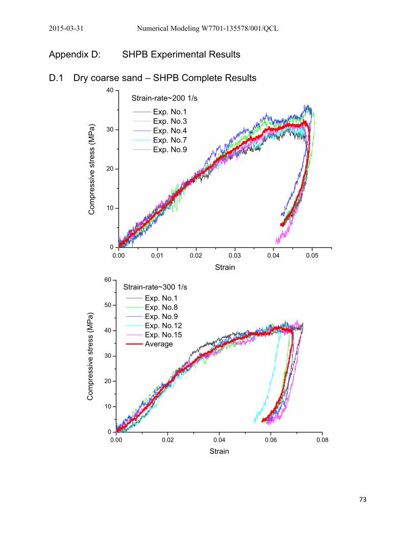
2015-03-31 Numerical Modeling W7701-135578/001/QCL
73
Appendix D: SHPB Experimental Results D.1 Dry coarse sand – SHPB Complete Results
0.00 0.01 0.02 0.03 0.04 0.050
10
20
30
40
Exp. No.1 Exp. No.3 Exp. No.4 Exp. No.7 Exp. No.9
Strain-rate~200 1/sC
ompr
essi
ve s
tress
(MP
a)
Strain
0.00 0.02 0.04 0.06 0.080
10
20
30
40
50
60
Exp. No.1 Exp. No.8 Exp. No.9 Exp. No.12 Exp. No.15 Average
Strain-rate~300 1/s
Com
pres
sive
stre
ss (M
Pa)
Strain
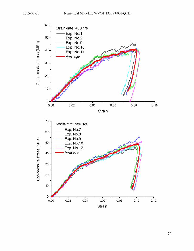
2015-03-31 Numerical Modeling W7701-135578/001/QCL
74
0.00 0.02 0.04 0.06 0.08 0.100
10
20
30
40
50
60
Exp. No.1 Exp. No.2 Exp. No.9 Exp. No.10 Exp. No.11 Average
Strain-rate~400 1/s
Com
pres
sive
stre
ss (M
Pa)
Strain
0.00 0.02 0.04 0.06 0.08 0.10 0.120
10
20
30
40
50
60
70
Exp. No.7 Exp. No.8 Exp. No.9 Exp. No.10 Exp. No.12 Average
Strain-rate~550 1/s
Com
pres
sive
stre
ss (M
Pa)
Strain
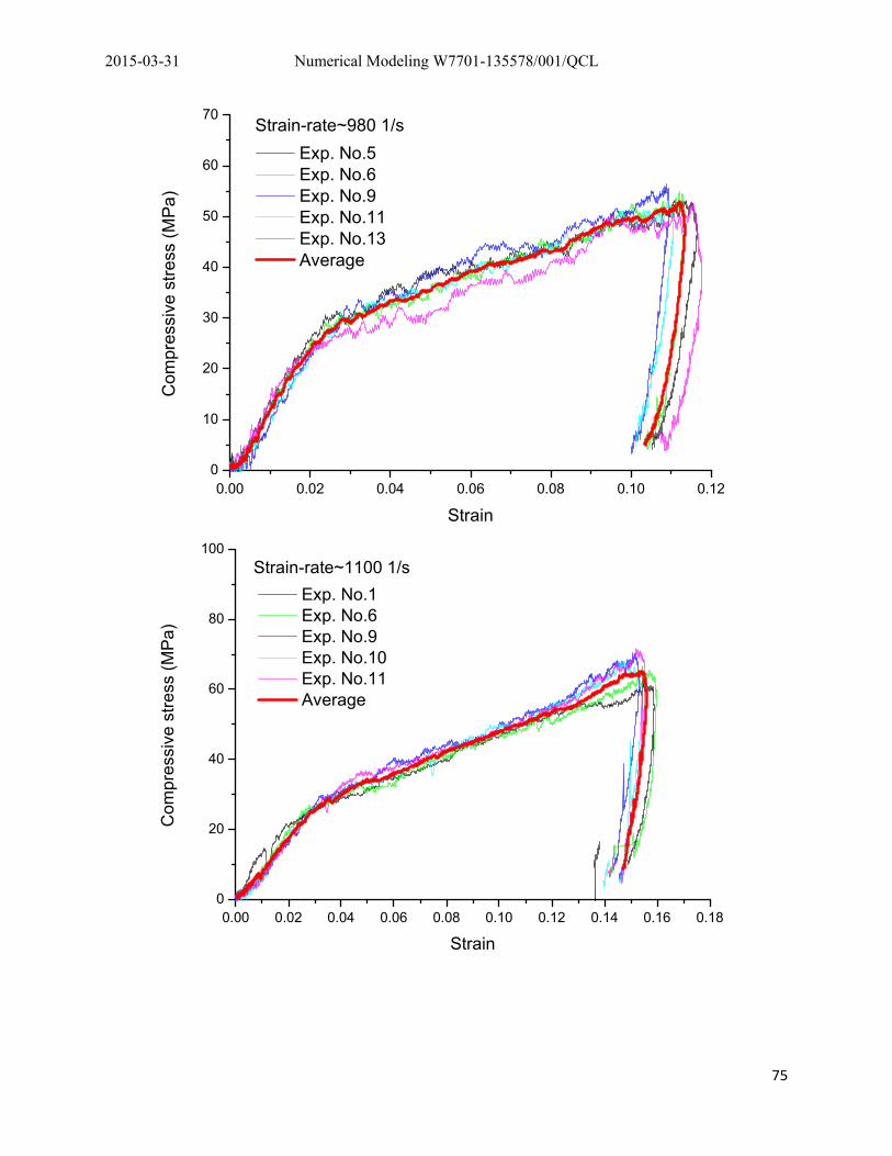
2015-03-31 Numerical Modeling W7701-135578/001/QCL
75
0.00 0.02 0.04 0.06 0.08 0.10 0.120
10
20
30
40
50
60
70
Exp. No.5 Exp. No.6 Exp. No.9 Exp. No.11 Exp. No.13 Average
Com
pres
sive
stre
ss (M
Pa)
Strain
Strain-rate~980 1/s
0.00 0.02 0.04 0.06 0.08 0.10 0.12 0.14 0.16 0.180
20
40
60
80
100
Exp. No.1 Exp. No.6 Exp. No.9 Exp. No.10 Exp. No.11 Average
Strain-rate~1100 1/s
Com
pres
sive
stre
ss (M
Pa)
Strain
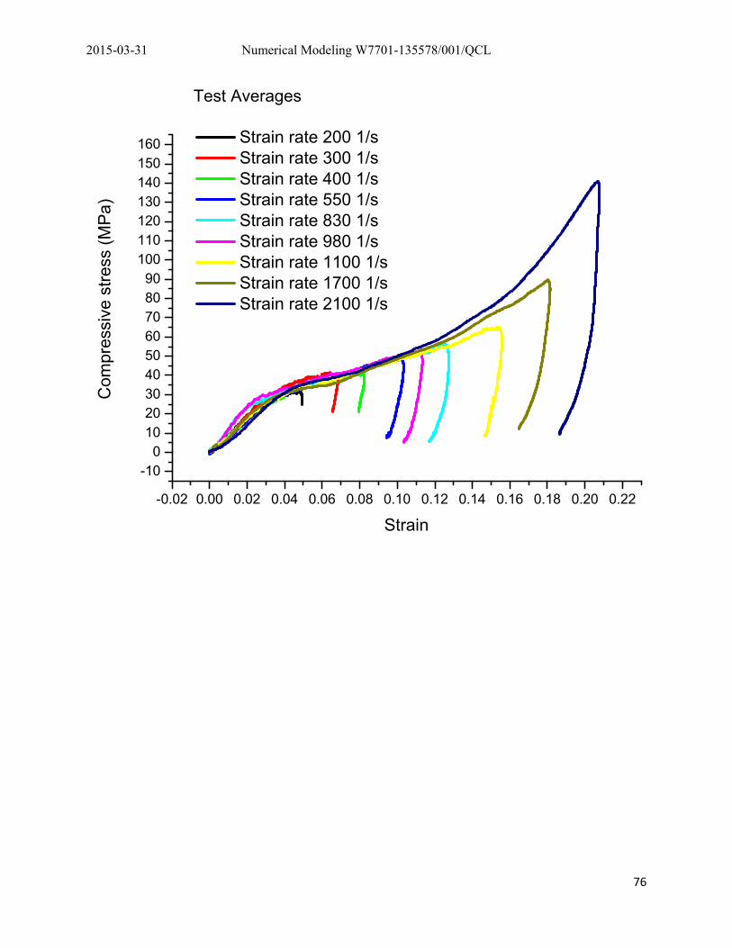
2015-03-31 Numerical Modeling W7701-135578/001/QCL
76
Test Averages
-0.02 0.00 0.02 0.04 0.06 0.08 0.10 0.12 0.14 0.16 0.18 0.20 0.22
-100
102030405060708090
100110120130140150160 Strain rate 200 1/s
Strain rate 300 1/s Strain rate 400 1/s Strain rate 550 1/s Strain rate 830 1/s Strain rate 980 1/s Strain rate 1100 1/s Strain rate 1700 1/s Strain rate 2100 1/s
Com
pres
sive
stre
ss (M
Pa)
Strain
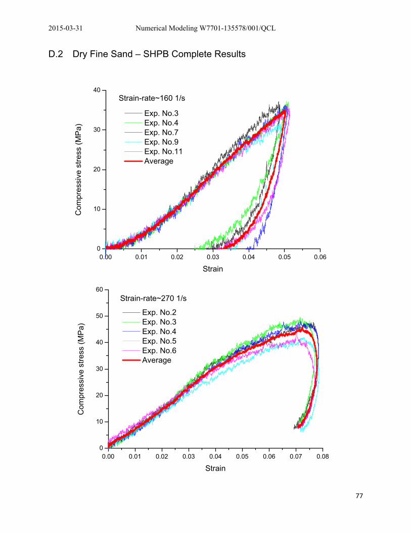
2015-03-31 Numerical Modeling W7701-135578/001/QCL
77
D.2 Dry Fine Sand – SHPB Complete Results
0.00 0.01 0.02 0.03 0.04 0.05 0.060
10
20
30
40
Exp. No.3 Exp. No.4 Exp. No.7 Exp. No.9 Exp. No.11 Average
Strain-rate~160 1/s
Com
pres
sive
stre
ss (M
Pa)
Strain
0.00 0.01 0.02 0.03 0.04 0.05 0.06 0.07 0.080
10
20
30
40
50
60
Exp. No.2 Exp. No.3 Exp. No.4 Exp. No.5 Exp. No.6 Average
Strain-rate~270 1/s
Com
pres
sive
stre
ss (M
Pa)
Strain
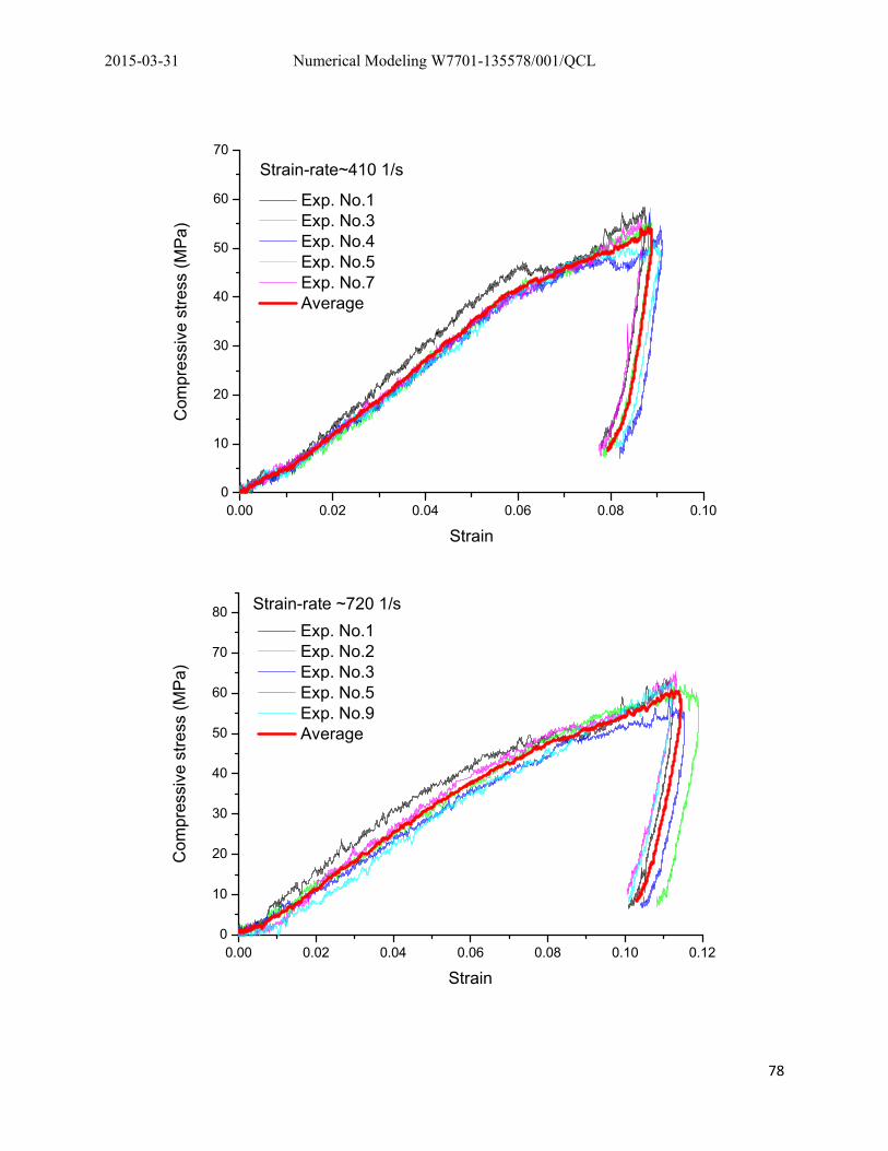
2015-03-31 Numerical Modeling W7701-135578/001/QCL
78
0.00 0.02 0.04 0.06 0.08 0.100
10
20
30
40
50
60
70
Exp. No.1 Exp. No.3 Exp. No.4 Exp. No.5 Exp. No.7 Average
Strain-rate~410 1/sC
ompr
essi
ve s
tress
(MP
a)
Strain
0.00 0.02 0.04 0.06 0.08 0.10 0.120
10
20
30
40
50
60
70
80 Exp. No.1 Exp. No.2 Exp. No.3 Exp. No.5 Exp. No.9 Average
Com
pres
sive
stre
ss (M
Pa)
Strain
Strain-rate ~720 1/s
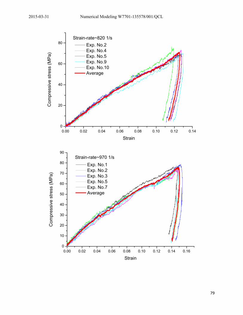
2015-03-31 Numerical Modeling W7701-135578/001/QCL
79
0.00 0.02 0.04 0.06 0.08 0.10 0.12 0.140
20
40
60
80 Exp. No.2 Exp. No.4 Exp. No.5 Exp. No.9 Exp. No.10 Average
Strain-rate~820 1/s
Com
pres
sive
stre
ss (M
Pa)
Strain
0.00 0.02 0.04 0.06 0.08 0.10 0.12 0.14 0.160
10
20
30
40
50
60
70
80
90
Exp. No.1 Exp. No.2 Exp. No.3 Exp. No.5 Exp. No.7 Average
Com
pres
sive
stre
ss (M
Pa)
Strain
Strain-rate~970 1/s
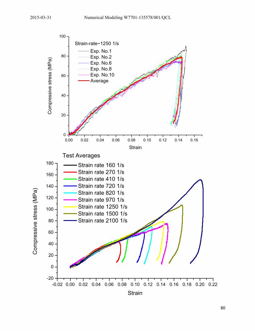
2015-03-31 Numerical Modeling W7701-135578/001/QCL
80
Test Averages
0.00 0.02 0.04 0.06 0.08 0.10 0.12 0.14 0.160
20
40
60
80
100
Exp. No.1 Exp. No.2 Exp. No.6 Exp. No.8 Exp. No.10 Average
Strain-rate~1250 1/sC
ompr
essi
ve s
tress
(MP
a)
Strain
-0.02 0.00 0.02 0.04 0.06 0.08 0.10 0.12 0.14 0.16 0.18 0.20 0.22-20
0
20
40
60
80
100
120
140
160
180 Strain rate 160 1/s Strain rate 270 1/s Strain rate 410 1/s Strain rate 720 1/s Strain rate 820 1/s Strain rate 970 1/s Strain rate 1250 1/s Strain rate 1500 1/s Strain rate 2100 1/s
Com
pres
sive
stre
ss (M
Pa)
Strain
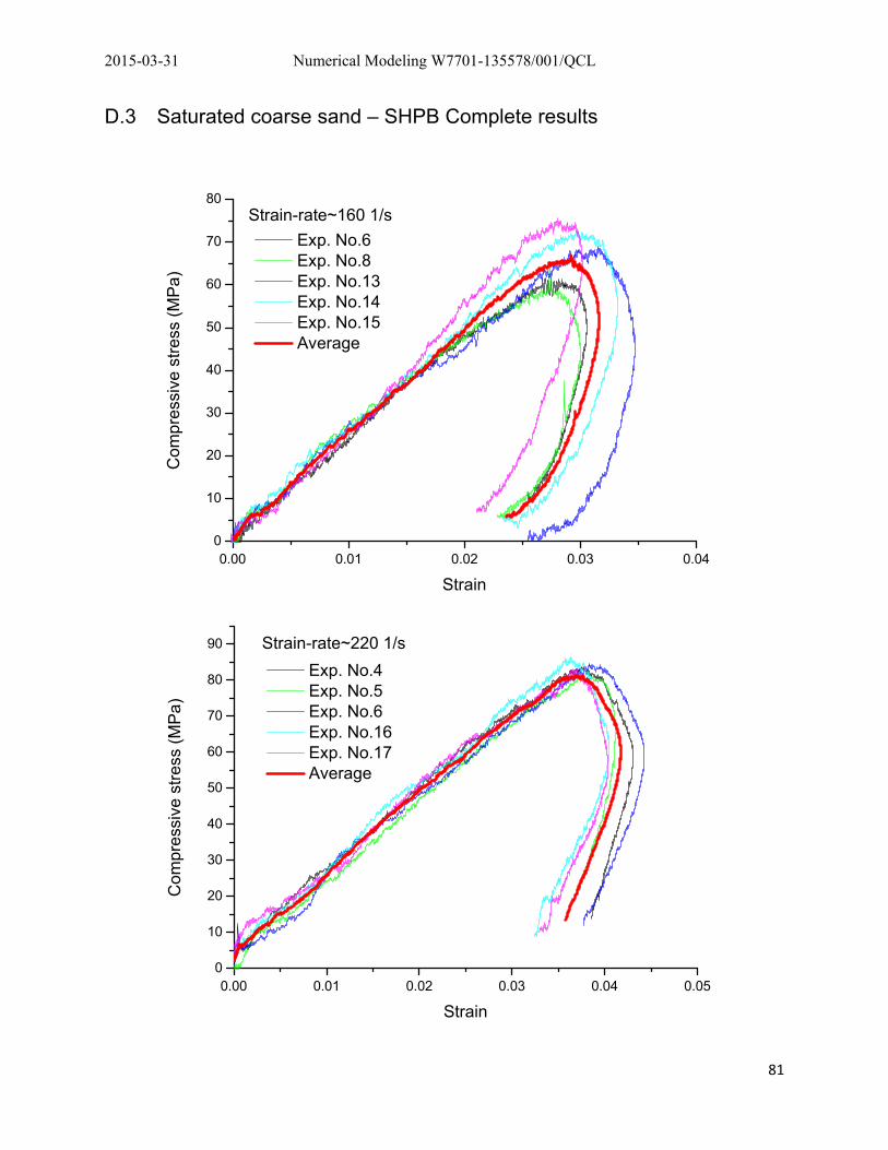
2015-03-31 Numerical Modeling W7701-135578/001/QCL
81
D.3 Saturated coarse sand – SHPB Complete results
0.00 0.01 0.02 0.03 0.040
10
20
30
40
50
60
70
80
Exp. No.6 Exp. No.8 Exp. No.13 Exp. No.14 Exp. No.15 Average
Strain-rate~160 1/s
Com
pres
sive
stre
ss (M
Pa)
Strain
0.00 0.01 0.02 0.03 0.04 0.050
10
20
30
40
50
60
70
80
90
Exp. No.4 Exp. No.5 Exp. No.6 Exp. No.16 Exp. No.17 Average
Strain-rate~220 1/s
Com
pres
sive
stre
ss (M
Pa)
Strain
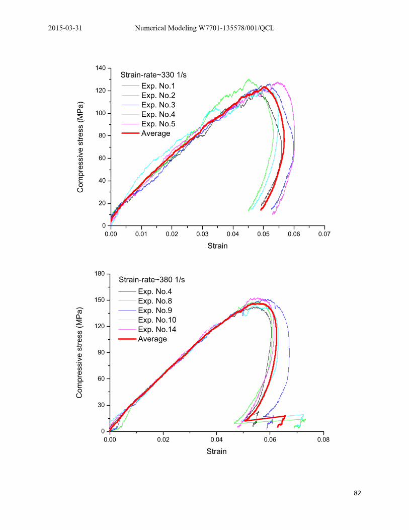
2015-03-31 Numerical Modeling W7701-135578/001/QCL
82
0.00 0.01 0.02 0.03 0.04 0.05 0.06 0.070
20
40
60
80
100
120
140
Exp. No.1 Exp. No.2 Exp. No.3 Exp. No.4 Exp. No.5 Average
Strain-rate~330 1/sC
ompr
essi
ve s
tress
(MP
a)
Strain
0.00 0.02 0.04 0.06 0.080
30
60
90
120
150
180
Exp. No.4 Exp. No.8 Exp. No.9 Exp. No.10 Exp. No.14 Average
Strain-rate~380 1/s
Com
pres
sive
stre
ss (M
Pa)
Strain
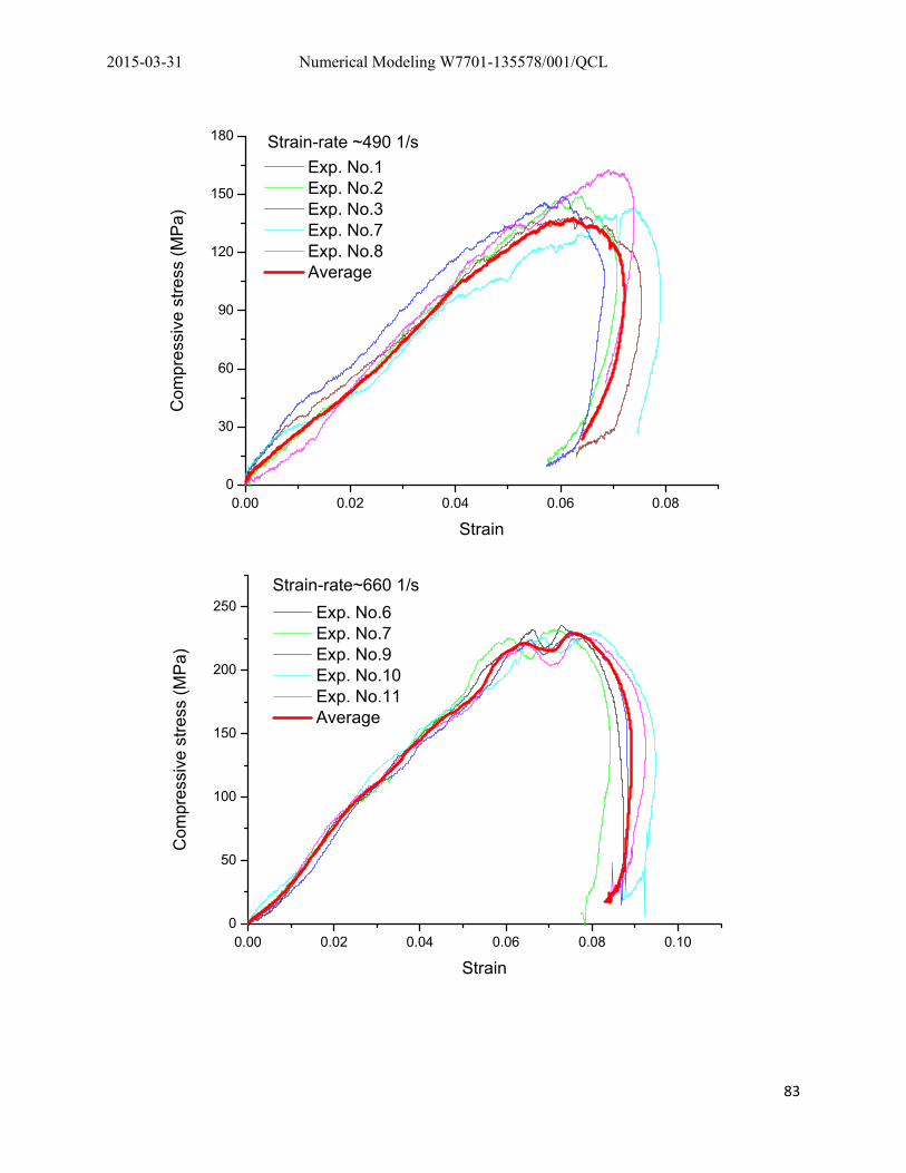
2015-03-31 Numerical Modeling W7701-135578/001/QCL
83
0.00 0.02 0.04 0.06 0.080
30
60
90
120
150
180
Exp. No.1 Exp. No.2 Exp. No.3 Exp. No.7 Exp. No.8 Average
Com
pres
sive
stre
ss (M
Pa)
Strain
Strain-rate ~490 1/s
0.00 0.02 0.04 0.06 0.08 0.100
50
100
150
200
250 Exp. No.6 Exp. No.7 Exp. No.9 Exp. No.10 Exp. No.11 Average
Com
pres
sive
stre
ss (M
Pa)
Strain
Strain-rate~660 1/s
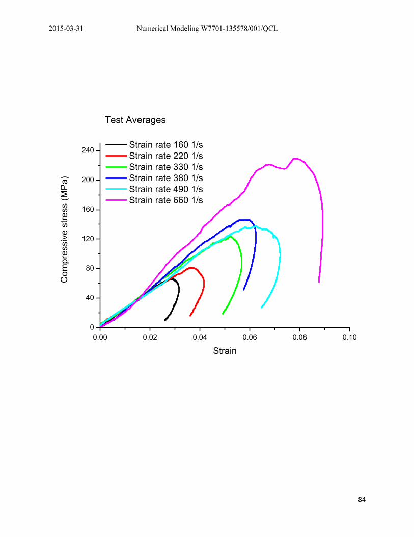
2015-03-31 Numerical Modeling W7701-135578/001/QCL
84
Test Averages
0.00 0.02 0.04 0.06 0.08 0.100
40
80
120
160
200
240 Strain rate 160 1/s Strain rate 220 1/s Strain rate 330 1/s Strain rate 380 1/s Strain rate 490 1/s Strain rate 660 1/s
Com
pres
sive
stre
ss (M
Pa)
Strain
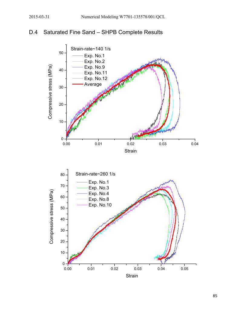
2015-03-31 Numerical Modeling W7701-135578/001/QCL
85
D.4 Saturated Fine Sand – SHPB Complete Results
0.00 0.01 0.02 0.03 0.040
10
20
30
40
50 Exp. No.1 Exp. No.2 Exp. No.9 Exp. No.11 Exp. No.12 Average
Strain-rate~140 1/sC
ompr
essi
ve s
tress
(MP
a)
Strain
0.00 0.01 0.02 0.03 0.04 0.050
10
20
30
40
50
60
70
80
Exp. No.1 Exp. No.3 Exp. No.4 Exp. No.8 Exp. No.10
Strain-rate~260 1/s
Com
pres
sive
stre
ss (M
Pa)
Strain
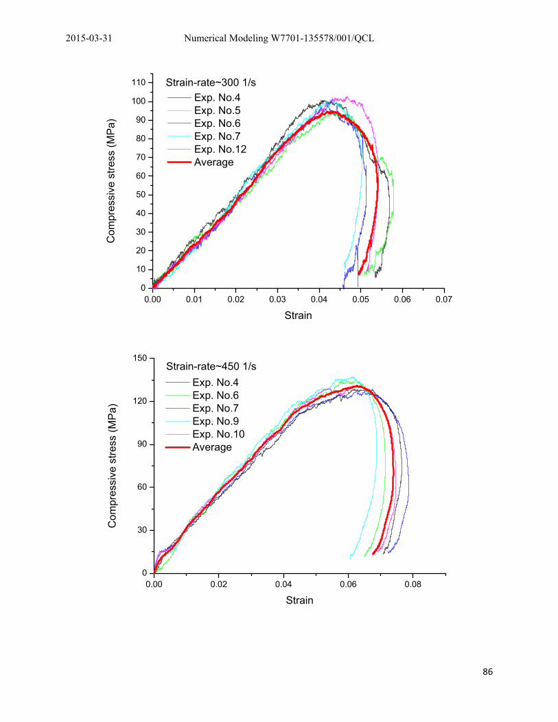
2015-03-31 Numerical Modeling W7701-135578/001/QCL
86
0.00 0.01 0.02 0.03 0.04 0.05 0.06 0.070
10
20
30
40
50
60
70
80
90
100
110
Exp. No.4 Exp. No.5 Exp. No.6 Exp. No.7 Exp. No.12 Average
Strain-rate~300 1/s
Com
pres
sive
stre
ss (M
Pa)
Strain
0.00 0.02 0.04 0.06 0.080
30
60
90
120
150
Exp. No.4 Exp. No.6 Exp. No.7 Exp. No.9 Exp. No.10 Average
Strain-rate~450 1/s
Com
pres
sive
stre
ss (M
Pa)
Strain
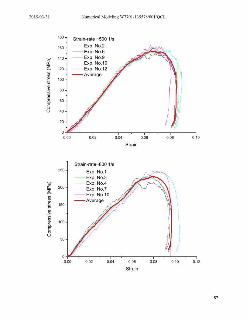
2015-03-31 Numerical Modeling W7701-135578/001/QCL
87
0.00 0.02 0.04 0.06 0.08 0.100
20
40
60
80
100
120
140
160
180
Exp. No.2 Exp. No.6 Exp. No.9 Exp. No.10 Exp. No.12 Average
Com
pres
sive
stre
ss (M
Pa)
Strain
Strain-rate ~500 1/s
0.00 0.02 0.04 0.06 0.08 0.10 0.120
50
100
150
200
250 Exp. No.1 Exp. No.3 Exp. No.4 Exp. No.7 Exp. No.10 Average
Com
pres
sive
stre
ss (M
Pa)
Strain
Strain-rate~800 1/s
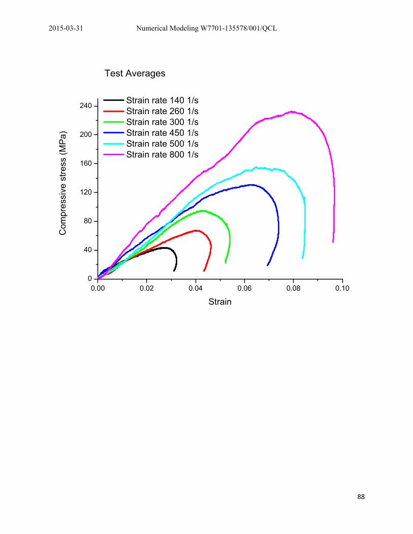
2015-03-31 Numerical Modeling W7701-135578/001/QCL
88
Test Averages
0.00 0.02 0.04 0.06 0.08 0.100
40
80
120
160
200
240 Strain rate 140 1/s Strain rate 260 1/s Strain rate 300 1/s Strain rate 450 1/s Strain rate 500 1/s Strain rate 800 1/s
Com
pres
sive
stre
ss (M
Pa)
Strain
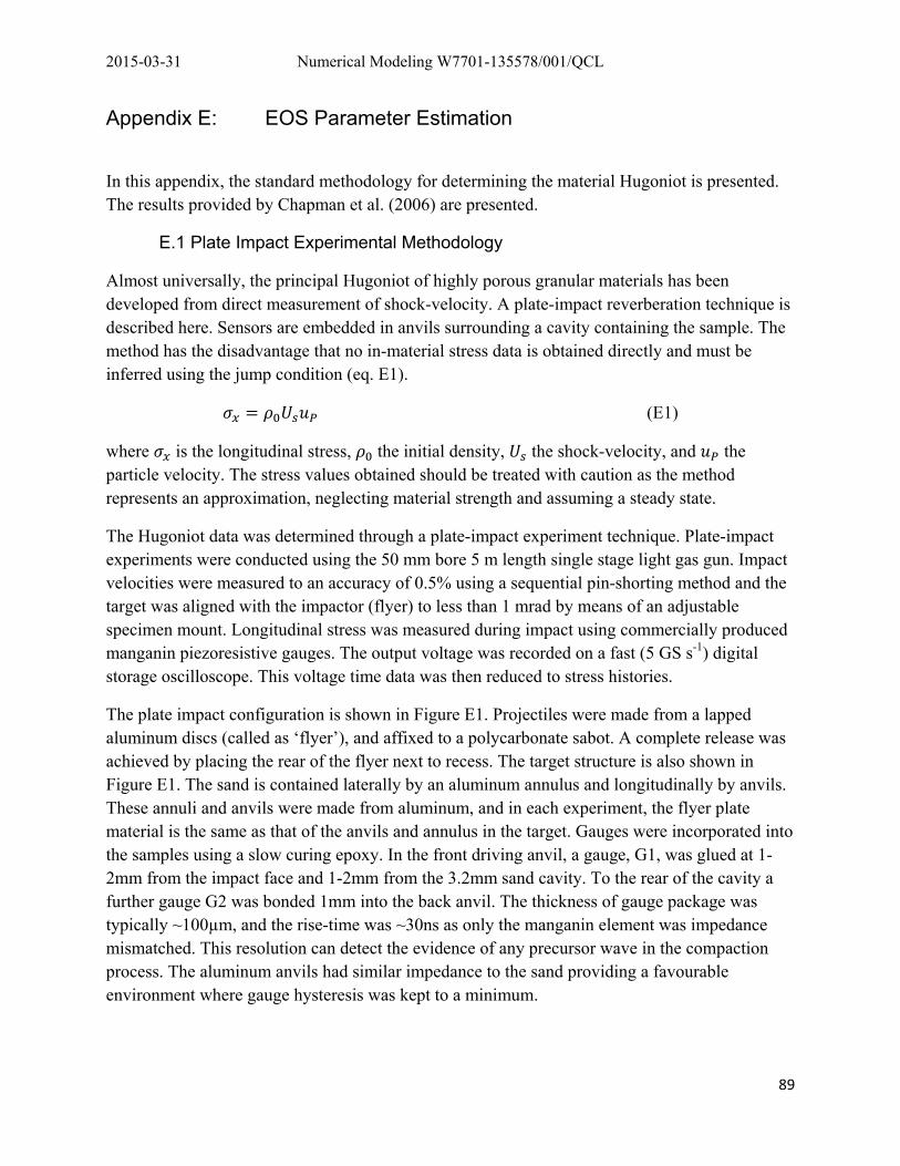
2015-03-31 Numerical Modeling W7701-135578/001/QCL
89
Appendix E: EOS Parameter Estimation
In this appendix, the standard methodology for determining the material Hugoniot is presented. The results provided by Chapman et al. (2006) are presented.
E.1 Plate Impact Experimental Methodology
Almost universally, the principal Hugoniot of highly porous granular materials has been developed from direct measurement of shock-velocity. A plate-impact reverberation technique is described here. Sensors are embedded in anvils surrounding a cavity containing the sample. The method has the disadvantage that no in-material stress data is obtained directly and must be inferred using the jump condition (eq. E1).
(E1)
where is the longitudinal stress, the initial density, the shock-velocity, and the particle velocity. The stress values obtained should be treated with caution as the method represents an approximation, neglecting material strength and assuming a steady state.
The Hugoniot data was determined through a plate-impact experiment technique. Plate-impact experiments were conducted using the 50 mm bore 5 m length single stage light gas gun. Impact velocities were measured to an accuracy of 0.5% using a sequential pin-shorting method and the target was aligned with the impactor (flyer) to less than 1 mrad by means of an adjustable specimen mount. Longitudinal stress was measured during impact using commercially produced manganin piezoresistive gauges. The output voltage was recorded on a fast (5 GS s-1) digital storage oscilloscope. This voltage time data was then reduced to stress histories.
The plate impact configuration is shown in Figure E1. Projectiles were made from a lapped aluminum discs (called as ‘flyer’), and affixed to a polycarbonate sabot. A complete release was achieved by placing the rear of the flyer next to recess. The target structure is also shown in Figure E1. The sand is contained laterally by an aluminum annulus and longitudinally by anvils. These annuli and anvils were made from aluminum, and in each experiment, the flyer plate material is the same as that of the anvils and annulus in the target. Gauges were incorporated into the samples using a slow curing epoxy. In the front driving anvil, a gauge, G1, was glued at 1-2mm from the impact face and 1-2mm from the 3.2mm sand cavity. To the rear of the cavity a further gauge G2 was bonded 1mm into the back anvil. The thickness of gauge package was typically ~100µm, and the rise-time was ~30ns as only the manganin element was impedance mismatched. This resolution can detect the evidence of any precursor wave in the compaction process. The aluminum anvils had similar impedance to the sand providing a favourable environment where gauge hysteresis was kept to a minimum.
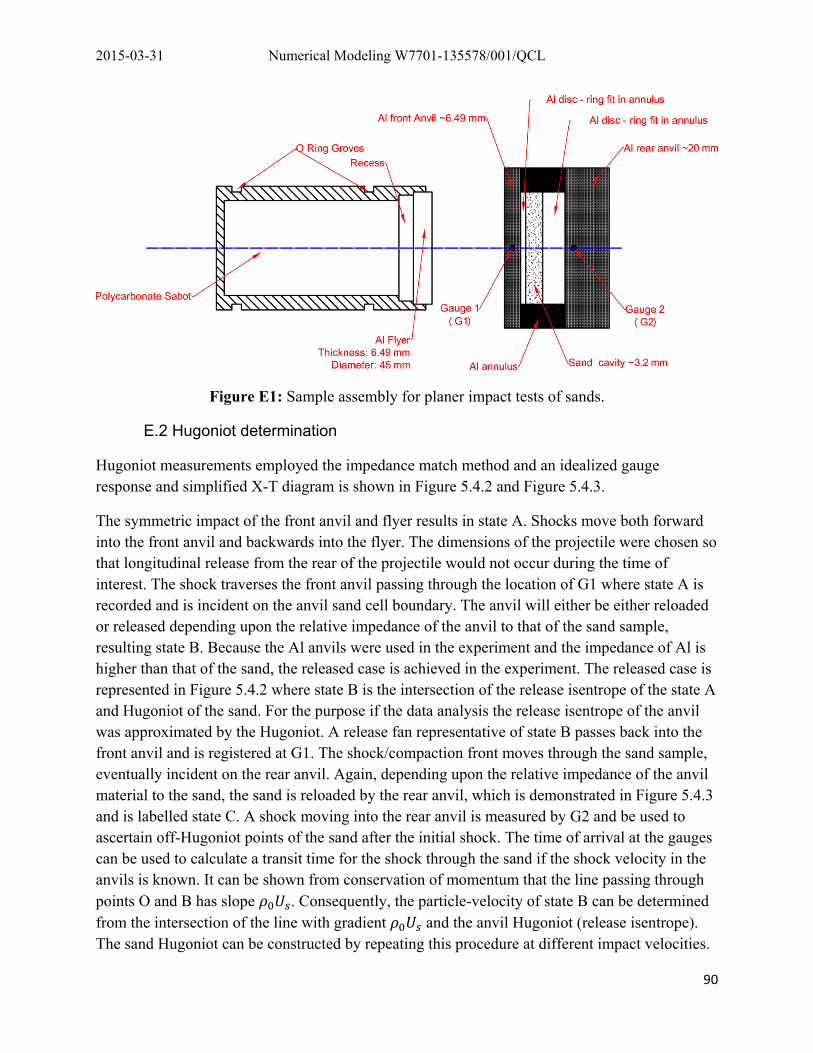
2015-03-31 Numerical Modeling W7701-135578/001/QCL
90
Figure E1: Sample assembly for planer impact tests of sands.
E.2 Hugoniot determination
Hugoniot measurements employed the impedance match method and an idealized gauge response and simplified X-T diagram is shown in Figure 5.4.2 and Figure 5.4.3.
The symmetric impact of the front anvil and flyer results in state A. Shocks move both forward into the front anvil and backwards into the flyer. The dimensions of the projectile were chosen so that longitudinal release from the rear of the projectile would not occur during the time of interest. The shock traverses the front anvil passing through the location of G1 where state A is recorded and is incident on the anvil sand cell boundary. The anvil will either be either reloaded or released depending upon the relative impedance of the anvil to that of the sand sample, resulting state B. Because the Al anvils were used in the experiment and the impedance of Al is higher than that of the sand, the released case is achieved in the experiment. The released case is represented in Figure 5.4.2 where state B is the intersection of the release isentrope of the state A and Hugoniot of the sand. For the purpose if the data analysis the release isentrope of the anvil was approximated by the Hugoniot. A release fan representative of state B passes back into the front anvil and is registered at G1. The shock/compaction front moves through the sand sample, eventually incident on the rear anvil. Again, depending upon the relative impedance of the anvil material to the sand, the sand is reloaded by the rear anvil, which is demonstrated in Figure 5.4.3 and is labelled state C. A shock moving into the rear anvil is measured by G2 and be used to ascertain off-Hugoniot points of the sand after the initial shock. The time of arrival at the gauges can be used to calculate a transit time for the shock through the sand if the shock velocity in the anvils is known. It can be shown from conservation of momentum that the line passing through points O and B has slope . Consequently, the particle-velocity of state B can be determined from the intersection of the line with gradient and the anvil Hugoniot (release isentrope). The sand Hugoniot can be constructed by repeating this procedure at different impact velocities.
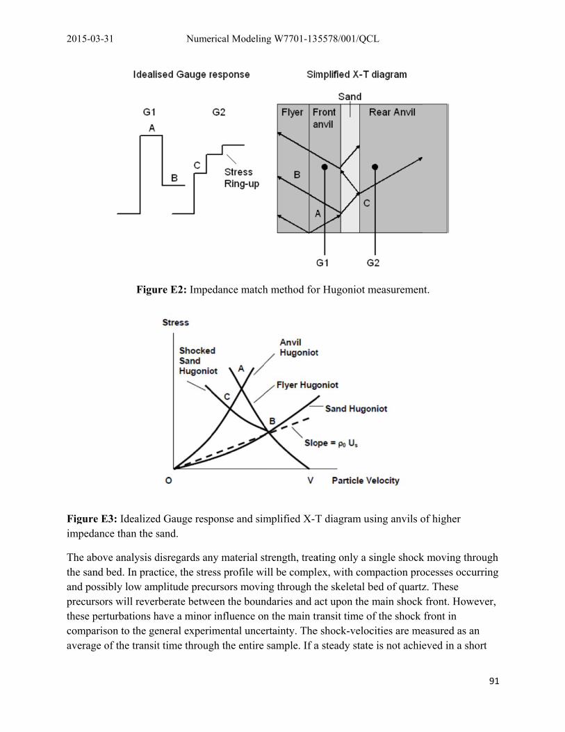
2015-03-3
Figure Eimpedanc
The abovthe sand and possiprecursorthese percomparisaverage o
31
Figur
E3: Idealizedce than the s
ve analysis dbed. In pracibly low amprs will reverbrturbations hson to the geof the transit
Numer
re E2: Impe
d Gauge respsand.
disregards antice, the streplitude precuberate betwe
have a minor eneral experit time throug
rical Modelin
edance match
ponse and sim
ny material sess profile wursors movineen the bouninfluence on
imental uncegh the entire
ng W7701-13
h method for
mplified X-T
strength, treaill be complng through tndaries and an the main tr
ertainty. Thesample. If a
5578/001/QC
r Hugoniot m
T diagram us
ating only a sex, with comthe skeletal bact upon the ransit time o
e shock-veloca steady state
CL
measuremen
sing anvils o
single shockmpaction probed of quartzmain shock
of the shock cities are mee is not achie
nt.
of higher
k moving throcesses occuz. These front. Howefront in
easured as aneved in a sho
91
rough urring
ever,
n ort
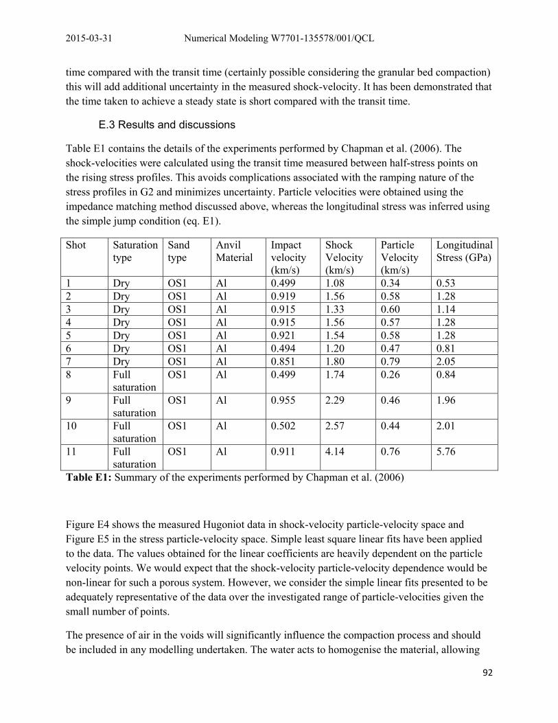
2015-03-31 Numerical Modeling W7701-135578/001/QCL
92
time compared with the transit time (certainly possible considering the granular bed compaction) this will add additional uncertainty in the measured shock-velocity. It has been demonstrated that the time taken to achieve a steady state is short compared with the transit time.
E.3 Results and discussions
Table E1 contains the details of the experiments performed by Chapman et al. (2006). The shock-velocities were calculated using the transit time measured between half-stress points on the rising stress profiles. This avoids complications associated with the ramping nature of the stress profiles in G2 and minimizes uncertainty. Particle velocities were obtained using the impedance matching method discussed above, whereas the longitudinal stress was inferred using the simple jump condition (eq. E1).
Shot Saturation type
Sand type
Anvil Material
Impact velocity (km/s)
Shock Velocity (km/s)
Particle Velocity (km/s)
Longitudinal Stress (GPa)
1 Dry OS1 Al 0.499 1.08 0.34 0.53 2 Dry OS1 Al 0.919 1.56 0.58 1.28 3 Dry OS1 Al 0.915 1.33 0.60 1.14 4 Dry OS1 Al 0.915 1.56 0.57 1.28 5 Dry OS1 Al 0.921 1.54 0.58 1.28 6 Dry OS1 Al 0.494 1.20 0.47 0.81 7 Dry OS1 Al 0.851 1.80 0.79 2.05 8 Full
saturation OS1 Al 0.499 1.74 0.26 0.84
9 Full saturation
OS1 Al 0.955 2.29 0.46 1.96
10 Full saturation
OS1 Al 0.502 2.57 0.44 2.01
11 Full saturation
OS1 Al 0.911 4.14 0.76 5.76
Table E1: Summary of the experiments performed by Chapman et al. (2006)
Figure E4 shows the measured Hugoniot data in shock-velocity particle-velocity space and Figure E5 in the stress particle-velocity space. Simple least square linear fits have been applied to the data. The values obtained for the linear coefficients are heavily dependent on the particle velocity points. We would expect that the shock-velocity particle-velocity dependence would be non-linear for such a porous system. However, we consider the simple linear fits presented to be adequately representative of the data over the investigated range of particle-velocities given the small number of points.
The presence of air in the voids will significantly influence the compaction process and should be included in any modelling undertaken. The water acts to homogenise the material, allowing
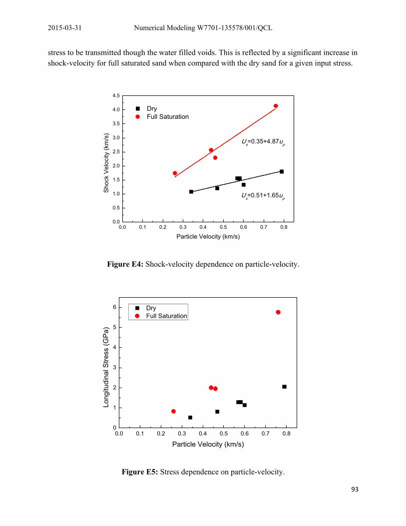
2015-03-31 Numerical Modeling W7701-135578/001/QCL
93
stress to be transmitted though the water filled voids. This is reflected by a significant increase in shock-velocity for full saturated sand when compared with the dry sand for a given input stress.
0.0 0.1 0.2 0.3 0.4 0.5 0.6 0.7 0.80.0
0.5
1.0
1.5
2.0
2.5
3.0
3.5
4.0
4.5
Us=0.35+4.87up
Shoc
k V
eloc
ity (k
m/s
)
Particle Velocity (km/s)
Dry Full Saturation
Us=0.51+1.65up
Figure E4: Shock-velocity dependence on particle-velocity.
0.0 0.1 0.2 0.3 0.4 0.5 0.6 0.7 0.80
1
2
3
4
5
6
Dry Full Saturation
Long
itudi
nal S
tress
(GP
a)
Particle Velocity (km/s)
Figure E5: Stress dependence on particle-velocity.
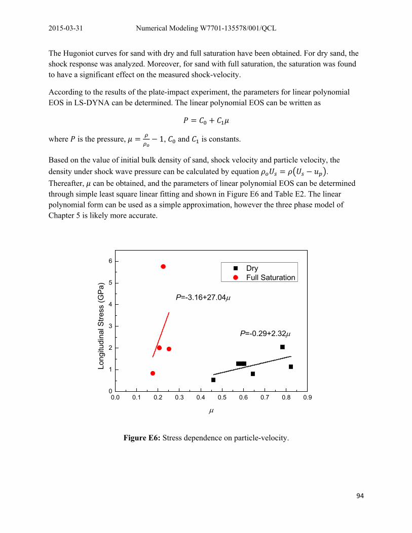
2015-03-31 Numerical Modeling W7701-135578/001/QCL
94
The Hugoniot curves for sand with dry and full saturation have been obtained. For dry sand, the shock response was analyzed. Moreover, for sand with full saturation, the saturation was found to have a significant effect on the measured shock-velocity.
According to the results of the plate-impact experiment, the parameters for linear polynomial EOS in LS-DYNA can be determined. The linear polynomial EOS can be written as
where is the pressure, 1, and is constants.
Based on the value of initial bulk density of sand, shock velocity and particle velocity, the
density under shock wave pressure can be calculated by equation .
Thereafter, can be obtained, and the parameters of linear polynomial EOS can be determined through simple least square linear fitting and shown in Figure E6 and Table E2. The linear polynomial form can be used as a simple approximation, however the three phase model of Chapter 5 is likely more accurate.
0.0 0.1 0.2 0.3 0.4 0.5 0.6 0.7 0.8 0.90
1
2
3
4
5
6
P=-3.16+27.04
P=-0.29+2.32
Long
itudi
nal S
tress
(GP
a)
Dry Full Saturation
Figure E6: Stress dependence on particle-velocity.

2015-03-31 Numerical Modeling W7701-135578/001/QCL
95
Dry -0.29 27.04 Full saturation -3.16 2.32 Table 5.4.2 The parameters of linear polynomial EOS.