Constant force extensional rheometry of polymer solutions

Journal of Non-Newtonian Fluid Mechanics 169–170 (2012) 26–41

Contents lists available at SciVerse ScienceDirect

Journal of Non-Newtonian Fluid Mechanics

journal homepage: ht tp : / /www.elsevier .com/locate / jnnfm

Constant force extensional rheometry of polymer solutions

Peter Szabo a,⇑, Gareth H. McKinley b, Christian Clasen c

a Department of Chemical and Biochemical Engineering, Technical University of Denmark, Søltofts Plads, Building 229, DK-2800 Kongens Lyngby, Denmarkb Department of Mechanical Engineering, Massachusetts Institute of Technology, Cambridge, MA 02139, USAc Department of Chemical Engineering, Katholieke Universiteit Leuven, Willem de Croylaan 46, 3001 Heverlee, Belgium

a r t i c l e i n f o a b s t r a c t

Article history:Received 17 September 2010Received in revised form 30 September2011Accepted 21 November 2011Available online 30 November 2011

Keywords:Extensional rheometryFilament stretchingPolymer solutionsExtensibility

0377-0257/$ - see front matter � 2011 Elsevier B.V. Adoi:10.1016/j.jnnfm.2011.11.003

⇑ Corresponding author.E-mail addresses: [email protected] (P. Szabo), garet

[email protected] (C. Clasen).

We revisit the rapid stretching of a liquid filament under the action of a constant imposed tensile force,a problem which was first considered by Matta and Tytus [J. Non-Newton. Fluid Mech. 35 (1990) 215–229]. A liquid bridge formed from a viscous Newtonian fluid or from a dilute polymer solution is firstestablished between two cylindrical disks. The upper disk is held fixed and may be connected to a forcetransducer while the lower cylinder falls due to gravity. By varying the mass of the falling cylinder andmeasuring its resulting acceleration, the viscoelastic nature of the elongating fluid filament can beprobed. In particular, we show that with this constant force pull (CFP) technique it is possible to readilyimpose very large material strains and strain rates so that the maximum extensibility of the polymermolecules may be quantified. This unique characteristic of the experiment is analyzed numericallyusing the FENE-P model and two alternative kinematic descriptions; employing either an axially-uni-form filament approximation or a quasi two-dimensional Lagrangian description of the elongatingthread. In addition, a second order pertubation theory for the trajectory of the falling mass is developedfor simple viscous filaments. Based on these theoretical considerations we develop an expression thatenables estimation of the finite extensibility parameter characterizing the polymer solution in terms ofquantities that can be extracted directly from simple measurement of the time-dependent filamentdiameter.

� 2011 Elsevier B.V. All rights reserved.

1. Introduction

The application of a constant force to stretch a viscoelastic li-quid sample in order to obtain material properties in extension isvery appealing since it simplifies the experimental approach signif-icantly. However, in comparison to shear rheometry in which thesurface area of a sample to which a force or torque is applied staysconstant, in a filament stretching extensional device the samplearea (on which a constant force acts) decreases (typically exponen-tially), resulting in a non-constant stress in the sample. Despitethese concerns, Chang and Lodge [5] have considered the theoret-ical implications of a constant force pull on a viscoelastic filamentin order to determine the ‘spinnability’ and stability of polymericliquids in uniaxial extension (due to the rapid approach towardslarge strains and the finite deformation limit of the polymer net-work). Matta and Tytus [28] provided the first experimental resultsof an extensional rheometry experiment using a constant forcepulling on a stretching liquid filament. Their approach utilized auniform cylindrical fluid sample held between two circular diskswith a weight attached to the lower plate which was then released

ll rights reserved.

[email protected] (G.H. McKinley),

and stretched the fluid filament with a constant gravitational forcepull. This groundbreaking work is the progenitor of the filamentstretching elongational rheometer (FSR or FiSER) that has beenused extensively for evaluating the transient rheometry of mobileliquids. The configuration used by Matta and Tytus [28] also moti-vates the experimental setup in the current paper which is de-picted in Fig. 1. The original apparatus described in [28] waslimited in the speed and optical resolution of the monitoring sys-tem and did not have the capability to directly measure the forcein the extending filament. In the present system we are able tomeasure the shape of the liquid column every 1/2000 second usinghigh speed video-imaging with a resolution of �72.3 lm/pixel atan image size of 512 � 1024 square pixel.

By using a suitable force balance that incorporated the gravita-tional body force and monitoring the filament diameter 2R, lengthL of the filament and the actual acceleration of the cylindricalweight, it was possible for Matta and Tytus [28] to calculate theforce (and thus the time-varying stress acting in the filament).However, they recognized that it was only possible to obtain‘apparent’ transient extensional viscosities as neither the extensionrate _� ¼ d ln L=dt nor the axial stress could directly be controlled orkept constant. As in the case of capillary breakup extensional rhe-ometry (CABER) [24,21,30,46,1,10], this constant force pull (CFP)technique is not viewed as a true rheometer but more as an

http://dx.doi.org/10.1016/j.jnnfm.2011.11.003

mailto:[email protected]



http://dx.doi.org/10.1016/j.jnnfm.2011.11.003

http://www.sciencedirect.com/science/journal/03770257

http://http://www.elsevier.com/locate/jnnfm

Fig. 1. Sequence of images of a polystyrene solution confined between two circular plates of radius R0 = 5.12 mm, stretched by a falling mass (m = 5.8155 g) that exerts aconstant force pull on the elongating filament over a distance of Lmax = 1.3 m. Time between consecutive images is Dt = 45 ms. The initial aspect ratio of the cylindrical fluidsample is K = L0/R0 = 0.4937. The first four images show the downwards accelerating stage used to initially hold and release the falling mass. The left hand vertical dashed linedepicts the point between images where the polymer stretch A approaches its finite extensibility limit b. The second vertical broken line indicates the limit up to which theradius at the axial mid-point L(t)/2 can still be directly observed.

P. Szabo et al. / Journal of Non-Newtonian Fluid Mechanics 169–170 (2012) 26–41 27

indexer for exploring and comparing the extensional behavior ofdifferent liquids. In a capillary thinning device, a thin liquid fila-ment of constant length is stretched beyond its Plateau stabilitylimit and the surface tension (rather than a falling weight) providesthe driving force to elongate a liquid filament. In this respect theCFP technique is somewhat more versatile as it allows one to ad-just the pulling force by varying the mass of the attached cylinder.

The groundbreaking work of Matta and Tytus [28] lead to thedevelopment of the filament stretching elongational rheometry,as it emphasized the need to develop stretching techniques that al-lowed one to control and set constant extension rates in order toobtain unambiguous measures of the transient and steady statematerial properties in uniaxial elongation. First results on filamentstretching with controlled uniaxial flow fields were reported by[45] and led to several designs of controlled filament stretchingrheometers (FSR) [2,29,3] that have been used extensively for eval-uating the transient extensional rheometry of mobile liquids.

For more viscous polymer melts, a number of extensional rhe-ometers were developed by Münstedt, Meissner and coworkerswell before the FSR (see [32] for a review). Devices such as thefilament stretching apparatus developed by Münstedt et al.[34,35] could rely on a number of assumptions such as negligibleeffects of capillarity and uniform deformation of molten poly-meric samples being elongated, as well as relatively slow stretch-ing dynamics, that allowed one to use realtime measurements offilament length and tensile force in order to impose constantrates or stresses. One important observation to note is that theuse of fast feedback loops (using the measured forces and fila-ment dimensions in order to determine and control the stress) al-lowed one to approach a steady state value of the stress muchfaster than with the controlled strain rates imposed in FSR de-vices [35]. Recently Sentmanat et al. [41] developed the Sentm-anat extensional rheometer (SER) fixture a device, that enablesextensional elongation of highly viscous samples with commer-cially available rotational rheometers. As in the Münstedt device,the SER relies on a controlled deformation applied at the rollers inorder to apply an approximately homogeneous strain in the sam-ple [15] and the resulting tensile stress (or resulting torque) isthen measured. These devices can also be operated in a constantextensional stress or ‘‘tensile creep’’ mode, by exponentiallyreducing the tensile force applied to the sample so that the ratioof the force to the time-varying cross-sectional area of the sampleremains constant. An interesting observation reported by bothMünstedt et al. [35] and by Sentmanat et al. [41] is that transientextensional rheology experiments operated in tensile creep modeapproach steady state more rapidly and at smaller total imposedstrain.

As we will show below, this is also true of the Matta and Tytusfalling weight experiment depicted in Fig. 1. This configurationthus provides a simple mechanism for imposing a controlled ten-sile load to a sample and reaching the steady state elongational vis-cosity more readily. However, of course, in this experiment it is theexternally imposed force that remains constant; the acceleration ofthe endplate and the total viscoelastic tensile stress exerted by thefluid test sample change as the filament elongates and thins.

In principle, the dripping of a viscoelastic liquid drop from anozzle can also be used in order to establish a constant tensile forceon the thinning filament connecting the pendant drop to the nozzle[18,19,42]. Jones et al. [17] used this geometry in conjunction withhigh speed imaging to explore transient extensional stress growthin the M1 test fluid. An approximate force balance showed that theapparent extensional viscosity could grow by two orders of magni-tude as the drop accelerated under gravity. A particularly interest-ing observation from this early work was that the calculatedvelocity curves showed the drop to accelerate, to decelerate andthen to accelerate again. We observe similar non-monotonicbehavior in the present experiments. Quantifying the kinematicsin the falling pendant drop experiment is challenging becausethe initial filament configuration is not well defined and the massof the end drop in general does not remain constant during eachexperiment, but can vary by up to 50% [17]. Furthermore, varia-tions in the tensile force can only be achieved by increasing thenozzle radius to create larger drops, but this invariably leads alsoto a larger initial radius of the filament and larger inertial effects.Analysis of the pendant drop experiment by Keiller [19] showedthat both viscous and elastic forces contributed significantly tothe thinning dynamics and complicated the use of this experimentas a true rheometer. The relatively low mass of a pendant drop (ascompared to the weights used by Matta and Tytus [28] and in thecurrent paper) also results in low imposed deformation rates; forexample, the maximum accelerations achieved by Jones et al. wereonly approximately �0.5 g. A recent detailed analysis of this prob-lem for the Maxwell/Oldroyd-B model shows that as the tensilestresses grow and retard further acceleration of the pendant drop-let and the elongating filament, the dynamics can in fact relax backtowards a dominant Newtonian balance [43] which again limitsthe use of this geometry as an extensional rheometer.

The recent analysis of Smolka et al. [43] highlights a keystrength of the CFP technique suggested by Matta and Tytus:Applying a high enough initial force allows one to impose filamentdeformation rates dln L/dt that are sufficiently fast to overcome therelaxation time k and the relaxation processes in the elongatingfluid filament. With Weissenberg numbers Wi = kdln L/dt� 1 theconstant force pull ultimately imposes an almost affine

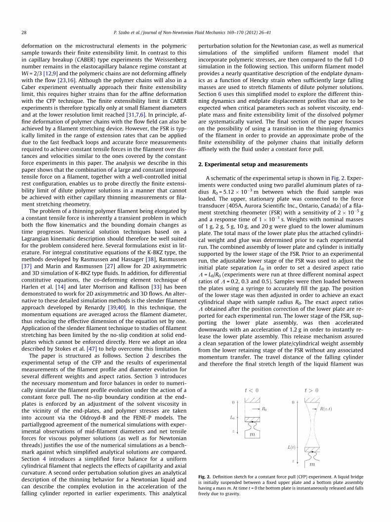
Fig. 2. Definition sketch for a constant force pull (CFP) experiment. A liquid bridgeis initially suspended between a fixed upper plate and a bottom plate assemblyhaving a mass m. At time t = 0 the bottom plate is instantaneously released and fallsfreely due to gravity.

28 P. Szabo et al. / Journal of Non-Newtonian Fluid Mechanics 169–170 (2012) 26–41

deformation on the microstructural elements in the polymericsample towards their finite extensibility limit. In contrast to thisin capillary breakup (CABER) type experiments the Weissenbergnumber remains in the elastocapillary balance regime constant atWi = 2/3 [12,9] and the polymeric chains are not deforming affinelywith the flow [23,16]. Although the polymer chains will also in aCaber experiment eventually approach their finite extensibilitylimit, this requires higher strains than for the affine deformationwith the CFP technique. The finite extensibility limit in CABERexperiments is therefore typically only at small filament diametersand at the lower resolution limit reached [31,7,6]. In principle, af-fine deformation of polymer chains with the flow field can also beachieved by a filament stretching device. However, the FSR is typ-ically limited in the range of extension rates that can be applieddue to the fast feedback loops and accurate force measurementsrequired to achieve constant tensile forces in the filament over dis-tances and velocities similar to the ones covered by the constantforce experiments in this paper. The analysis we describe in thispaper shows that the combination of a large and constant imposedtensile force on a filament, together with a well-controlled initialrest configuration, enables us to probe directly the finite extensi-bility limit of dilute polymer solutions in a manner that cannotbe achieved with either capillary thinning measurements or fila-ment stretching rheometry.

The problem of a thinning polymer filament being elongated bya constant tensile force is inherently a transient problem in whichboth the flow kinematics and the bounding domain changes astime progresses. Numerical solution techniques based on aLagrangian kinematic description should therefore be well suitedfor the problem considered here. Several formulations exist in lit-erature. For integral constitutive equations of the K-BKZ type, themethods developed by Rasmussen and Hassager [38], Rasmussen[37] and Marin and Rasmussen [27] allow for 2D axisymmetricand 3D simulation of K-BKZ type fluids. In addition, for differentialconstitutive equations, the co-deforming element technique ofHarlen et al. [14] and later Morrison and Rallison [33] has beendemonstrated to work for 2D axisymmetric and 3D flows. An alter-native to these detailed simulation methods is the slender filamentapproach developed by Renardy [39,40]. In this technique, themomentum equations are averaged across the filament diameter,thus reducing the effective dimension of the equation set by one.Application of the slender filament technique to studies of filamentstretching has been limited by the no-slip condition at solid end-plates which cannot be enforced directly. Here we adopt an ideadescribed by Stokes et al. [47] to help overcome this limitation.

The paper is structured as follows. Section 2 describes theexperimental setup of the CFP and the results of experimentalmeasurements of the filament profile and diameter evolution forseveral different weights and aspect ratios. Section 3 introducesthe necessary momentum and force balances in order to numeri-cally simulate the filament profile evolution under the action of aconstant force pull. The no-slip boundary condition at the end-plates is enforced by an adjustment of the solvent viscosity inthe vicinity of the end-plates, and polymer stresses are takeninto account via the Oldroyd-B and the FENE-P models. Thepartiallygood agreement of the numerical simulations with exper-imental observations of mid-filament diameters and net tensileforces for viscous polymer solutions (as well as for Newtonianthreads) justifies the use of the numerical simulations as a bench-mark against which simplified analytical solutions are compared.Section 4 introduces a simplified force balance for a uniformcylindrical filament that neglects the effects of capillarity and axialcurvature. A second order pertubation solution gives an analyticaldescription of the thinning behavior for a Newtonian liquid andcan describe the complex evolution in the acceleration of thefalling cylinder reported in earlier experiments. This analytical

perturbation solution for the Newtonian case, as well as numericalsimulations of the simplified uniform filament model thatincorporate polymeric stresses, are then compared to the full 1-Dsimulation in the following section. This uniform filament modelprovides a nearly quantitative description of the endplate dynam-ics as a function of Hencky strain when sufficiently large fallingmasses are used to stretch filaments of dilute polymer solutions.Section 6 uses this simplified model to explore the different thin-ning dynamics and endplate displacement profiles that are to beexpected when critical parameters such as solvent viscosity, end-plate mass and finite extensibility limit of the dissolved polymerare systematically varied. The final section of the paper focuseson the possibility of using a transition in the thinning dynamicsof the filament in order to provide an approximate probe of thefinite extensibility of the polymer chains that initially deformaffinely with the fluid under a constant force pull.

2. Experimental setup and measurements

A schematic of the experimental setup is shown in Fig. 2. Exper-iments were conducted using two parallel aluminum plates of ra-dius R0 = 5.12 � 10�3 m between which the fluid sample wasloaded. The upper, stationary plate was connected to the forcetransducer (405A, Aurora Scientific Inc., Ontario, Canada) of a fila-ment stretching rheometer (FSR) with a sensitivity of 2 � 10�5 gand a response time of 1� 10�3 s. Weights with nominal massesof 1 g, 2 g, 5 g, 10 g, and 20 g were glued to the lower aluminumplate. The total mass of the lower plate plus the attached cylindri-cal weight and glue was determined prior to each experimentalrun. The combined assembly of lower plate and cylinder is initiallysupported by the lower stage of the FSR. Prior to an experimentalrun, the adjustable lower stage of the FSR was used to adjust theinitial plate separation L0 in order to set a desired aspect ratioK = L0/R0 (experiments were run at three different nominal aspectratios of K = 0.2, 0.3 and 0.5). Samples were then loaded betweenthe plates using a syringe to accurately fill the gap. The positionof the lower stage was then adjusted in order to achieve an exactcylindrical shape with sample radius R0. The exact aspect ratiosK obtained after the position correction of the lower plate are re-ported for each experimental run. The lower stage of the FSR, sup-porting the lower plate assembly, was then accelerateddownwards with an acceleration of 1.2 g in order to instantly re-lease the lower plate assembly. This release mechanism assureda clean separation of the lower plate/cylindrical weight assemblyfrom the lower retaining stage of the FSR without any associatedmomentum transfer. The travel distance of the falling cylinderand therefore the final stretch length of the liquid filament was

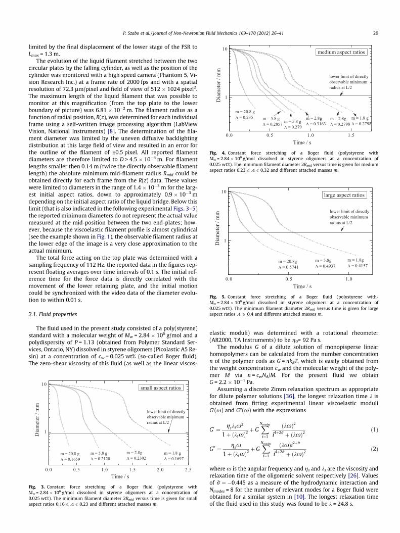
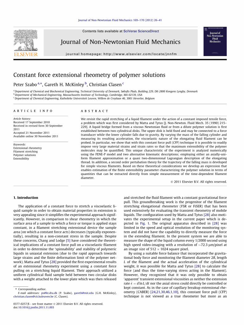
Fig. 4. Constant force stretching of a Boger fluid (polystyrene withMw = 2.84 � 106 g/mol dissolved in styrene oligomers at a concentration of0.025 wt%). The minimum filament diameter 2Rmid versus time is given for mediumaspect ratios 0.23 6K 6 0.32 and different attached masses m.

Fig. 5. Constant force stretching of a Boger fluid (polystyrene with-Mw = 2.84 � 106 g/mol dissolved in styrene oligomers at a concentration of0.025 wt%). The minimum filament diameter 2Rmid versus time is given for largeaspect ratios K P 0.4 and different attached masses m.


limited by the final displacement of the lower stage of the FSR toLmax = 1.3 m.

The evolution of the liquid filament stretched between the twocircular plates by the falling cylinder, as well as the position of thecylinder was monitored with a high speed camera (Phantom 5, Vi-sion Research Inc.) at a frame rate of 2000 fps and with a spatialresolution of 72.3 lm/pixel and field of view of 512 � 1024 pixel2.The maximum length of the liquid filament that was possible tomonitor at this magnification (from the top plate to the lowerboundary of picture) was 6.81 � 10�2 m. The filament radius as afunction of radial position, R(z), was determined for each individualframe using a self-written image processing algorithm (LabViewVision, National Instruments) [8]. The determination of the fila-ment diameter was limited by the uneven diffusive backlightingdistribution at this large field of view and resulted in an error forthe outline of the filament of ±0.5 pixel. All reported filamentdiameters are therefore limited to D > 4.5 � 10�4 m. For filamentlengths smaller then 0.14 m (twice the directly observable filamentlength) the absolute minimum mid-filament radius Rmid could beobtained directly for each frame from the R(z) data. These valueswere limited to diameters in the range of 1.4 � 10�3 m for the larg-est initial aspect ratios, down to approximately 0.9 � 10�3 mdepending on the initial aspect ratio of the liquid bridge. Below thislimit (that is also indicated in the following experimental Figs. 3–5)the reported minimum diameters do not represent the actual valuemeasured at the mid-position between the two end-plates; how-ever, because the viscoelastic filament profile is almost cylindrical(see the example shown in Fig. 1), the observable filament radius atthe lower edge of the image is a very close approximation to theactual minimum.

The total force acting on the top plate was determined with asampling frequency of 112 Hz, the reported data in the figures rep-resent floating averages over time intervals of 0.1 s. The initial ref-erence time for the force data is directly correlated with themovement of the lower retaining plate, and the initial motioncould be synchronized with the video data of the diameter evolu-tion to within 0.01 s.

2.1. Fluid properties

The fluid used in the present study consisted of a poly(styrene)standard with a molecular weight of Mw = 2.84 � 106 g/mol and apolydispersity of P = 1.13 (obtained from Polymer Standard Ser-vices, Ontario, NY) dissolved in styrene oligomers (Picolastic A5 Re-sin) at a concentration of cw = 0.025 wt% (so-called Boger fluid).The zero-shear viscosity of this fluid (as well as the linear viscos-

Fig. 3. Constant force stretching of a Boger fluid (polystyrene withMw = 2.84 � 106 g/mol dissolved in styrene oligomers at a concentration of0.025 wt%). The minimum filament diameter 2Rmid versus time is given for smallaspect ratios 0.16 6K 6 0.23 and different attached masses m.

elastic moduli) was determined with a rotational rheometer(AR2000, TA Instruments) to be g0= 92 Pa s.

The modulus G of a dilute solution of monopisperse linearhomopolymers can be calculated from the number concentrationn of the polymer coils as G = nkBT, which is easily obtained fromthe weight concentration cw and the molecular weight of the poly-mer M via n = cwNA/M. For the present fluid we obtainG = 2.2 � 10�1 Pa.

Assuming a discrete Zimm relaxation spectrum as appropriatefor dilute polymer solutions [36], the longest relaxation time k isobtained from fitting experimental linear viscoelastic moduliG0(x) and G00(x) with the expressions

G0 ¼ gsksx2

1þ ðksxÞ2þ G

XNmodes

i¼1

ðkxÞ2

i4þ2~r þ ðkxÞ2ð1Þ

G00 ¼ gsx1þ ðksxÞ2

þ GXNmodes

i¼1

ðkxÞi2þ~r

i4þ2~r þ ðkxÞ2ð2Þ

where x is the angular frequency and gs and ks are the viscosity andrelaxation time of the oligomeric solvent respectively [26]. Valuesof ~r ¼ �0:445 as a measure of the hydrodynamic interaction andNmodes = 8 for the number of relevant modes for a Boger fluid wereobtained for a similar system in [10]. The longest relaxation timeof the fluid used in this study was found to be k = 24.8 s.

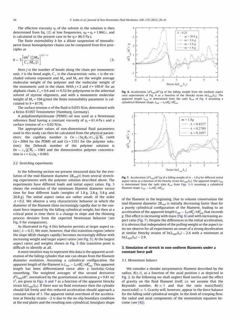
Fig. 6. Acceleration (d2Lapp/dt2)/g of the falling weight from the medium aspectratio experiments of Fig. 4 as a function of the Hencky strain ln(Lapp/L0). Theapparent length Lapp is determined from the radii Rmid of Fig. 4 assuming acylindrical filament shape, Lapp ¼ L0pR2

0=pR2mid .

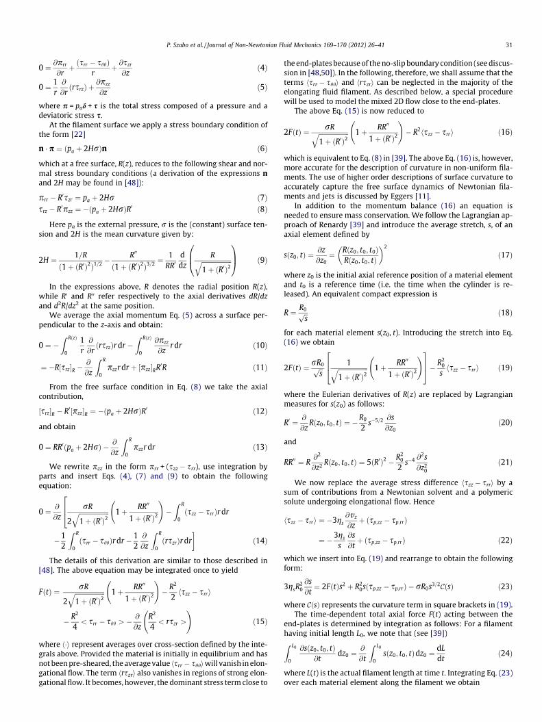
Fig. 7. Acceleration (d2Lapp/dt2)/g of a falling weight of m � 1.8 g for different initialaspect ratios as a function of the Hencky strain ln(Lapp/L0). The apparent length Lapp

is determined from the radii data Rmid from Figs. 3–5 assuming a cylindricalfilament shape, Lapp ¼ L0pR2

0=pR2mid .


The effective viscosity gs of the solvent in the solution is thendetermined from Eq. (2) at low frequencies, g0 = gs + 1.86Gk, andis calculated in the present case to be gs= 86.5 Pa s.

The finite extensibility b for a dilute suspension of monodis-perse linear homopolymer chains can be computed from first prin-ciples as

b ¼ 3sin2 h

2

� �Mw

C1ðMu=jÞ

" #2ð1�mÞ

ð3Þ

Here j is the number of bonds along the chain per monomericunit, h is the bond angle, C1 is the characteristic ratio, m is the ex-cluded volume exponent and Mw and Mu are the weight averagemolecular weight of the polymer and the molecular weight ofthe monomeric unit in the chain. With j = 2 and h = 109.4� for analiphatic chain, C1= 9.6 and m= 0.52 for polystyrene in the athermalsolvent of styrene oligomers, and with a monomeric molecularweight of Mu = 104 g/mol the finite extensibility parameter is cal-culated to b = 8176.

The surface tension r of the fluid is 0.035 N/m, determined witha Krüss K10ST Tensiometer (Hamburg, Germany).

A polydimethylsiloxane (PDMS) oil was used as a Newtonianreference fluid having a constant viscosity of gs = 61.4 Pa s and asurface tension of r = 0.02 N/m.

The appropriate values of non-dimensional fluid parametersused in this study can then be calculated from the physical param-eters: the capillary number is Ca ¼ ð3gsR0=rÞ

ffiffiffiffiffiffiffiffiffiffig=R0

p(with

Ca = 2064 for the PDMS oil and Ca = 1551 for the polymer solu-tion); the Deborah number of the polymer solution isDe ¼ k


p¼ 1085 and the dimensionless polymer concentra-

tion is c = Gk/gs = 0.063.

2.2. Stretching experiments

In the following section we present measured data for the evo-lution of the mid-filament diameter 2Rmid(t) from several stretch-ing experiments with the polymer solution described above. Theexperiments have different loads and initial aspect ratios. Fig. 3shows the evolution of the minimum filament diameter versustime for four different loads (weights of 1.8 g, 2.8 g, 5.8 g and20.8 g). The initial aspect ratios are rather small; of the orderK = 0.2. We observe a very characteristic behavior in which thediameter of the filament thins increasingly rapidly due to the con-stant force imposed by the falling cylindrical weight, but then at acritical point in time there is a change in slope and the thinningprocess deviates from the expected Newtonian behavior (seeFig. 9 for comparison).

As illustrated in Fig. 4 this behavior persists at larger aspect ra-tios (K ’ 0.3). We note, however, that this transition region (wherethe slope dR/dt changes rapidly) becomes increasingly diffuse withincreasing weight and larger aspect ratios (see Fig. 5). At the largestaspect ratios and weights shown in Fig. 5 this transition point isdifficult to identify at all.

A more intuitive way to represent this data is the apparent accel-eration of the falling cylinder that one can obtain from the filamentdiameter evolution. Assuming a cylindrical configuration theapparent length of the filament is Lapp ¼ L0pR2

0=pR2mid. This apparent

length has been differentiated twice after a Savitzky–Golaysmoothing. The weighted averages of this second derivatived2Lapp/dt2, normalized by the gravitational acceleration g = 9.81 m/s2, are given in Figs. 6 and 7 as a function of the apparent Henckystrain ln(Lapp/L0). If there was no fluid resistance then the cylindershould fall freely and this reduced acceleration should approach aconstant value of 1. The apparent initial overshoot of the accelera-tion at Hencky strains �2 is due to the no-slip boundary conditionat the end plates and the resulting non-cylindrical, hourglass shape

of the filament in the beginning. Due to volume conservation themid-filament diameter 2Rmid is initially decreasing faster than fora purely cylindrical configuration of the filament, leading to anacceleration of the apparent length Lapp ¼ L0pR2

0=pR2mid that exceeds

g. This effect is increasing with mass (Fig. 6) and with increasing as-pect ratio (Fig. 7). Despite the differences in the initial acceleration,it is obvious that independent of the pulling weight or the aspect ra-tio we observe for all experiments an onset of a strong decelerationat similar Hencky strains of ln(Lapp/L0) � 2.4 with a minimum atln(Lapp/L0) � 2.9.

3. Simulation of stretch in non-uniform filaments under aconstant force pull

3.1. Momentum balance

We consider a slender axisymmetric filament described by theradius, R(z, t), as a function of the axial position z as depicted inFig. 2. In the following we shall neglect fluid inertia and the effectof gravity on the fluid filament itself, i.e. we assume that theReynolds number, Re� 1 and that the ratio mass(fluid)/mass(solid)� 1. Gravity will, however, appear in the force balancefor the falling solid cylindrical weight. In the limit of creeping flow,the radial and axial components of the momentum equation be-come (see [4]):


0 ¼ @prr

@rþ ðsrr � shhÞ

rþ @szr

@zð4Þ

0 ¼ 1r@

@rðrsrzÞ þ

@pzz

@zð5Þ

where p = pad + s is the total stress composed of a pressure and adeviatoric stress s.

At the filament surface we apply a stress boundary condition ofthe form [22]

n � p ¼ ðpa þ 2HrÞn ð6Þ

which at a free surface, R(z), reduces to the following shear and nor-mal stress boundary conditions (a derivation of the expressions nand 2H may be found in [48]):

prr � R0szr ¼ pa þ 2Hr ð7Þsrz � R0pzz ¼ �ðpa þ 2HrÞR0 ð8Þ

Here pa is the external pressure, r is the (constant) surface ten-sion and 2H is the mean curvature given by:

2H ¼ 1=R

ð1þ ðR0Þ2Þ1=2 �R00

ð1þ ðR0Þ2Þ3=2 ¼1

RR0ddz

Rffiffiffiffiffiffiffiffiffiffiffiffiffiffiffiffiffiffiffi1þ ðR0Þ2

q0B@

1CA ð9Þ

In the expressions above, R denotes the radial position R(z),while R0 and R00 refer respectively to the axial derivatives dR/dzand d2R/dz2 at the same position.

We average the axial momentum Eq. (5) across a surface per-pendicular to the z-axis and obtain:

0 ¼ �Z RðzÞ

0

1r@

@rðrsrzÞr dr �

Z RðzÞ

0

@pzz

@zr dr ð10Þ

¼ �R½srz�R �@

@z

Z R

0pzzr dr þ ½pzz�RR0R ð11Þ

From the free surface condition in Eq. (8) we take the axialcontribution,

½srz�R � R0½pzz�R ¼ �ðpa þ 2HrÞR0 ð12Þ

and obtain

0 ¼ RR0ðpa þ 2HrÞ � @

@z

Z R

0pzzr dr ð13Þ

We rewrite pzz in the form prr + (szz � srr), use integration byparts and insert Eqs. (4), (7) and (9) to obtain the followingequation:

0 ¼ @

@zrR

2ffiffiffiffiffiffiffiffiffiffiffiffiffiffiffiffiffiffiffi1þ ðR0Þ2

q 1þ RR00

1þ ðR0Þ2

!�Z R

0ðszz � srrÞr dr

264

�12

Z R

0ðsrr � shhÞr dr � 1

2@

@z

Z R

0ðrszrÞr dr

�ð14Þ

The details of this derivation are similar to those described in[48]. The above equation may be integrated once to yield

FðtÞ ¼ rR

2ffiffiffiffiffiffiffiffiffiffiffiffiffiffiffiffiffiffiffi1þ ðR0Þ2

q 1þ RR00

1þ ðR0Þ2

!� R2

2hszz � srri

� R2

4< srr � shh > �

@

@zR2

4< rszr >

!ð15Þ

where h�i represent averages over cross-section defined by the inte-grals above. Provided the material is initially in equilibrium and hasnot been pre-sheared, the average value hsrr � shhiwill vanish in elon-gational flow. The term hrszri also vanishes in regions of strong elon-gational flow. It becomes, however, the dominant stress term close to

the end-plates because of the no-slip boundary condition (see discus-sion in [48,50]). In the following, therefore, we shall assume that theterms hsrr � shhi and hrszri can be neglected in the majority of theelongating fluid filament. As described below, a special procedurewill be used to model the mixed 2D flow close to the end-plates.

The above Eq. (15) is now reduced to

2FðtÞ ¼ rRffiffiffiffiffiffiffiffiffiffiffiffiffiffiffiffiffiffiffi1þ ðR0Þ2

q 1þ RR00

1þ ðR0Þ2

!� R2hszz � srri ð16Þ

which is equivalent to Eq. (8) in [39]. The above Eq. (16) is, however,more accurate for the description of curvature in non-uniform fila-ments. The use of higher order descriptions of surface curvature toaccurately capture the free surface dynamics of Newtonian fila-ments and jets is discussed by Eggers [11].

In addition to the momentum balance (16) an equation isneeded to ensure mass conservation. We follow the Lagrangian ap-proach of Renardy [39] and introduce the average stretch, s, of anaxial element defined by

sðz0; tÞ ¼@z@z0¼ Rðz0; t0; t0Þ

Rðz0; t0; tÞ

� �2

ð17Þ

where z0 is the initial axial reference position of a material elementand t0 is a reference time (i.e. the time when the cylinder is re-leased). An equivalent compact expression is

R ¼ R0ffiffisp ð18Þ

for each material element s(z0, t). Introducing the stretch into Eq.(16) we obtain

2FðtÞ ¼ rR0ffiffisp 1ffiffiffiffiffiffiffiffiffiffiffiffiffiffiffiffiffiffiffi

1þ ðR0Þ2q 1þ RR00

1þ ðR0Þ2

!264

375� R2

0

shszz � srri ð19Þ

where the Eulerian derivatives of R(z) are replaced by Lagrangianmeasures for s(z0) as follows:

R0 ¼ @

@zRðz0; t0; tÞ ¼ �

R0

2s�5=2 @s

@z0ð20Þ

and

RR00 ¼ R@2

@z2 Rðz0; t0; tÞ ¼ 5ðR0Þ2 � R20

2s�4 @

2s@z2

0

ð21Þ

We now replace the average stress difference hszz � srri by asum of contributions from a Newtonian solvent and a polymericsolute undergoing elongational flow. Hence

hszz � srri ¼ �3gs@vz

@zþ ðsp;zz � sp;rrÞ

¼ �3gs

s@s@tþ ðsp;zz � sp;rrÞ ð22Þ

which we insert into Eq. (19) and rearrange to obtain the followingform:

3gsR20@s@t¼ 2FðtÞs2 þ R2

0sðsp;zz � sp;rrÞ � rR0s3=2CðsÞ ð23Þ

where CðsÞ represents the curvature term in square brackets in (19).The time-dependent total axial force F(t) acting between the

end-plates is determined by integration as follows: For a filamenthaving initial length L0, we note that (see [39])Z L0

0

@sðz0; t0; tÞ@t

dz0 ¼@

@t

Z L0

0sðz0; t0; tÞdz0 ¼

dLdt

ð24Þ

where L(t) is the actual filament length at time t. Integrating Eq. (23)over each material element along the filament we obtain


2FðtÞ ¼

R L00 rR0s3=2CðsÞ � R2

0sðsp;zz � sp;rrÞn o

dz0 þ 3gsR20

dLdtR L0

0 s2 dz0

ð25Þ

A similar expression was given in [26]. The evolution of the fil-ament is determined from the combined solution of Eq. (23) foreach material element s(z0, t) and (25) for the total force over allmaterial elements, in conjunction with the force balance for a con-stant force pull and a viscoelastic constitutive equation withappropriate boundary and initial conditions. The discretization isuniform in the Lagrangian co-ordinate z0 with typically 800–1600 elements along the filament.

3.2. Force balance

The global force balance necessary to solve for the evolution ofthe filament is obtained from the experimentally-observable accel-eration of the lower endplate/mass assembly shown in Fig. 1. Theacceleration, described by the actual filament length d2L/dt2, isdetermined by the gravitational acceleration of the endplateassembly mass m and the resisting force F(t) (Eq. (25)) in the fila-ment. Newton’s second law for the falling mass can then be writtenin the form:

md2Ldt2 ¼ mg � FðtÞ ð26Þ

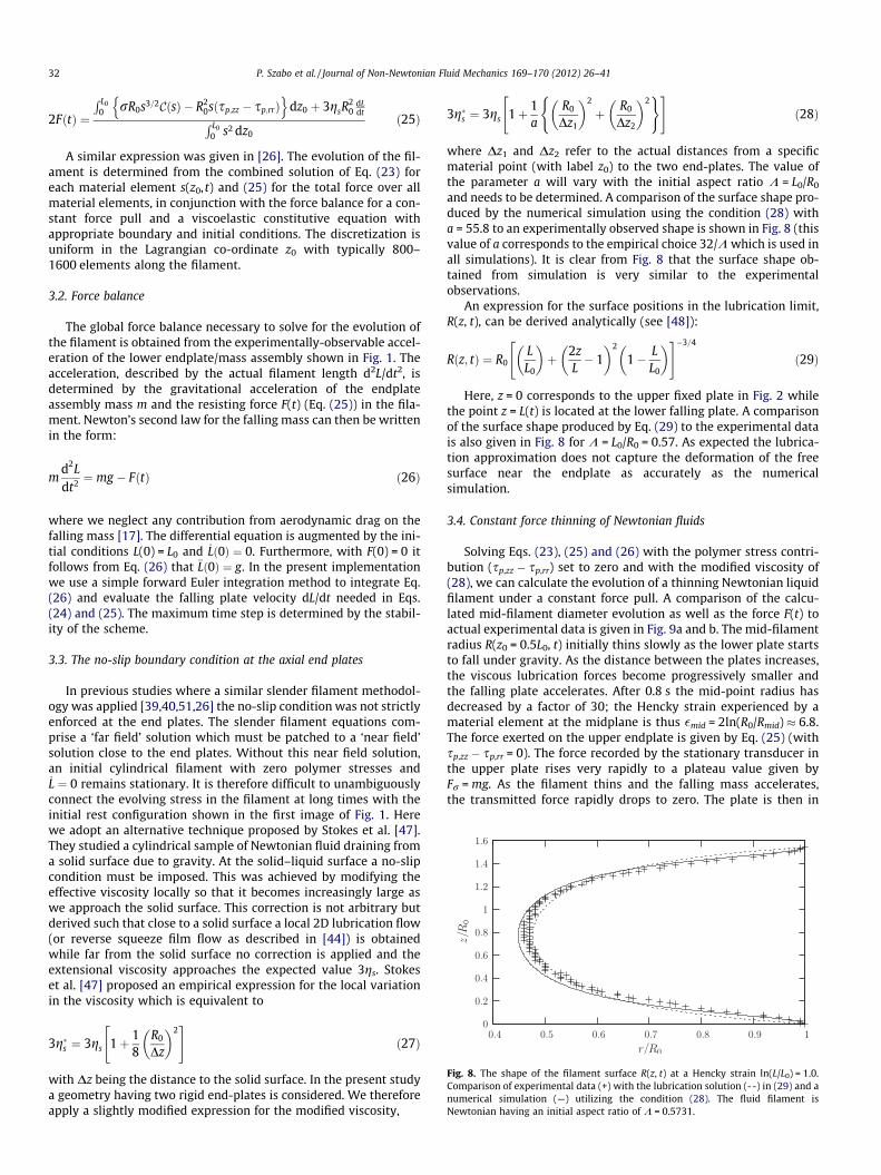
Fig. 8. The shape of the filament surface R(z, t) at a Hencky strain ln(L/L0) = 1.0.Comparison of experimental data (+) with the lubrication solution (--) in (29) and anumerical simulation (—) utilizing the condition (28). The fluid filament isNewtonian having an initial aspect ratio of K = 0.5731.

where we neglect any contribution from aerodynamic drag on thefalling mass [17]. The differential equation is augmented by the ini-tial conditions L(0) = L0 and _Lð0Þ ¼ 0. Furthermore, with F(0) = 0 itfollows from Eq. (26) that €Lð0Þ ¼ g. In the present implementationwe use a simple forward Euler integration method to integrate Eq.(26) and evaluate the falling plate velocity dL/dt needed in Eqs.(24) and (25). The maximum time step is determined by the stabil-ity of the scheme.

3.3. The no-slip boundary condition at the axial end plates

In previous studies where a similar slender filament methodol-ogy was applied [39,40,51,26] the no-slip condition was not strictlyenforced at the end plates. The slender filament equations com-prise a ‘far field’ solution which must be patched to a ‘near field’solution close to the end plates. Without this near field solution,an initial cylindrical filament with zero polymer stresses and_L ¼ 0 remains stationary. It is therefore difficult to unambiguouslyconnect the evolving stress in the filament at long times with theinitial rest configuration shown in the first image of Fig. 1. Herewe adopt an alternative technique proposed by Stokes et al. [47].They studied a cylindrical sample of Newtonian fluid draining froma solid surface due to gravity. At the solid–liquid surface a no-slipcondition must be imposed. This was achieved by modifying theeffective viscosity locally so that it becomes increasingly large aswe approach the solid surface. This correction is not arbitrary butderived such that close to a solid surface a local 2D lubrication flow(or reverse squeeze film flow as described in [44]) is obtainedwhile far from the solid surface no correction is applied and theextensional viscosity approaches the expected value 3gs. Stokeset al. [47] proposed an empirical expression for the local variationin the viscosity which is equivalent to

3gs ¼ 3gs 1þ 18

R0

Dz

� �2" #

ð27Þ

with Dz being the distance to the solid surface. In the present studya geometry having two rigid end-plates is considered. We thereforeapply a slightly modified expression for the modified viscosity,

3gs ¼ 3gs 1þ 1a

R0

Dz1

� �2

þ R0

Dz2

� �2( )" #

ð28Þ

where Dz1 and Dz2 refer to the actual distances from a specificmaterial point (with label z0) to the two end-plates. The value ofthe parameter a will vary with the initial aspect ratio K = L0/R0

and needs to be determined. A comparison of the surface shape pro-duced by the numerical simulation using the condition (28) witha = 55.8 to an experimentally observed shape is shown in Fig. 8 (thisvalue of a corresponds to the empirical choice 32/K which is used inall simulations). It is clear from Fig. 8 that the surface shape ob-tained from simulation is very similar to the experimentalobservations.

An expression for the surface positions in the lubrication limit,R(z, t), can be derived analytically (see [48]):

Rðz; tÞ ¼ R0LL0

� �þ 2z

L� 1

� �2

1� LL0

� �" #�3=4

ð29Þ

Here, z = 0 corresponds to the upper fixed plate in Fig. 2 whilethe point z = L(t) is located at the lower falling plate. A comparisonof the surface shape produced by Eq. (29) to the experimental datais also given in Fig. 8 for K = L0/R0 = 0.57. As expected the lubrica-tion approximation does not capture the deformation of the freesurface near the endplate as accurately as the numericalsimulation.

3.4. Constant force thinning of Newtonian fluids

Solving Eqs. (23), (25) and (26) with the polymer stress contri-bution (sp,zz � sp,rr) set to zero and with the modified viscosity of(28), we can calculate the evolution of a thinning Newtonian liquidfilament under a constant force pull. A comparison of the calcu-lated mid-filament diameter evolution as well as the force F(t) toactual experimental data is given in Fig. 9a and b. The mid-filamentradius R(z0 = 0.5L0, t) initially thins slowly as the lower plate startsto fall under gravity. As the distance between the plates increases,the viscous lubrication forces become progressively smaller andthe falling plate accelerates. After 0.8 s the mid-point radius hasdecreased by a factor of 30; the Hencky strain experienced by amaterial element at the midplane is thus �mid = 2ln(R0/Rmid) 6.8.The force exerted on the upper endplate is given by Eq. (25) (withsp,zz � sp,rr = 0). The force recorded by the stationary transducer inthe upper plate rises very rapidly to a plateau value given byFr = mg. As the filament thins and the falling mass accelerates,the transmitted force rapidly drops to zero. The plate is then in

(a)

(b)

Fig. 9. Comparison of experimental data with numerical simulation of the constantforce pull for (a) the mid-point diameter of an elongating filament and (b) the forcemeasured at the upper endplate with the force FðtÞ ¼ mg �m€L from Eq. (25). TheNewtonian test fluid is a viscous PDMS oil with gs = 61.4 Pa s and r = 0.02 N/m,m = 2.8 g. The corresponding dimensionless parameters (defined in Section 4.1) areV = 11.56, Ca = 2064, K = 0.4781.

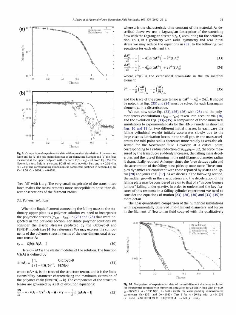
Fig. 10. Comparison of experimental data of the mid-filament diameter evolutionfor the polymer solution with numerical simulation for a FENE-P fluid with b = 800,gs = 86.5 Pa s, r = 0.035 N/m, k = 24.8 s (with the corresponding dimensionlessparameters Ca = 1551 and De = 1085): Test I for m = 20.8 g with K = 0.1659


‘free fall’ with €L ¼ g. The very small magnitude of the transmittedforce makes the measurements more susceptible to noise than di-rect observations of the filament radius.

3.5. Polymer solutions

When the liquid filament connecting the falling mass to the sta-tionary upper plate is a polymer solution we need to incorporatethe polymeric stresses (sp,zz � sp,rr) in (23) and (25) that were ne-glected in the previous section. For dilute polymer solutions weconsider the elastic stresses predicted by the Oldroyd-B andFENE-P models (see [4] for reference). We may express the compo-nents of the polymer stress in terms of the non-dimensional struc-ture tensor A:

sp ¼ �G½hðtrAÞA� I� ð30Þ

Here G = nkT is the elastic modulus of the solution. The functionh(trA) is defined by

hðtrAÞ ¼1; Oldroyd-Bð1� trA=bÞ�1

; FENE-P

�ð31Þ

where trA = Aii is the trace of the structure tensor, and b is the finiteextensibility parameter characterizing the maximum extension ofthe polymer chain (lim(trA) ? b). The components of the structuretensor are governed by a set of evolution equations:

@A@tþ v � rA�rvT � A� A � rv ¼ �1

k½hðtrAÞA� I� ð32Þ

where k is the characteristic time constant of the material. As de-scribed above we use a Lagrangian description of the stretchingflow with the Lagrangian stretch s(z0, t) accounting for the deforma-tion. Thus, in a geometry with radial symmetry and zero initialstress we may reduce the equations in (32) to the following twoequations for each element (i):

dAðiÞrr

dt¼ 1

k1� AðiÞrr hðtrAðiÞÞh i

� _�ðiÞðtÞAðiÞrr ð33Þ

dAðiÞzz

dt¼ 1

k1� AðiÞzz hðtrAðiÞÞh i

þ 2 _�ðiÞðtÞAðiÞzz ð34Þ

where _�ðiÞðtÞ is the extensional strain-rate in the ith materialelement

_�ðiÞ ¼ �2R

@R@t

� �z0

¼ 1s

@s@t

� �z0

ð35Þ

and the trace of the structure tensor is trAðiÞ ¼ AðiÞzz þ 2AðiÞrr . It shouldbe noted that Eqs. (33) and (34) must be solved for each Lagrangianelement z0 in a discretisation.

We can now solve Eqs. (23), (25), (26) with (28) and the poly-mer stress contribution (sp,zz � sp,rr) taken into account via (30)and the evolution Eqs. (33)–(35). A comparison of these numericalsimulations to experimental data for the FENE-P model is shown inFigs. 10 and 11 for two different initial masses. In each case thefalling cylindrical weight initially accelerates slowly due to thelarge viscous lubrication forces in the small gap. As the mass accel-erates, the mid-point radius decreases more rapidly as was also ob-served for the Newtonian fluid. However, at a critical point,corresponding to a radius reduction of Rmid/R0 � 0.2, the force mea-sured by the transducer suddenly increases, the falling mass decel-erates and the rate of thinning in the mid-filament diameter radiusis dramatically reduced. At longer times the force decays again andthe acceleration of the falling mass picks up once more. These com-plex dynamics are consistent with those reported by Matta and Ty-tus [28] and Jones et al. [17]. As we discuss in the following section,the sudden growth in the elastic stress and the deceleration of thefalling plate may be considered as akin to that of a ‘‘viscous bungeejumper’’ falling under gravity. In order to understand the key fea-tures of this response in a falling cylinder experiment we need toconsider the equations of motion (23)–(28), (30) and (33)–(35) inmore detail.

The near quantitative comparison of the numerical simulationswith experimentally observed mid-filament diameters and forcesin the filament of Newtonian fluid coupled with the qualitatively

(V = 0.761); and Test II for m = 5.8 g with K = 0.2120 (V = 3.47).

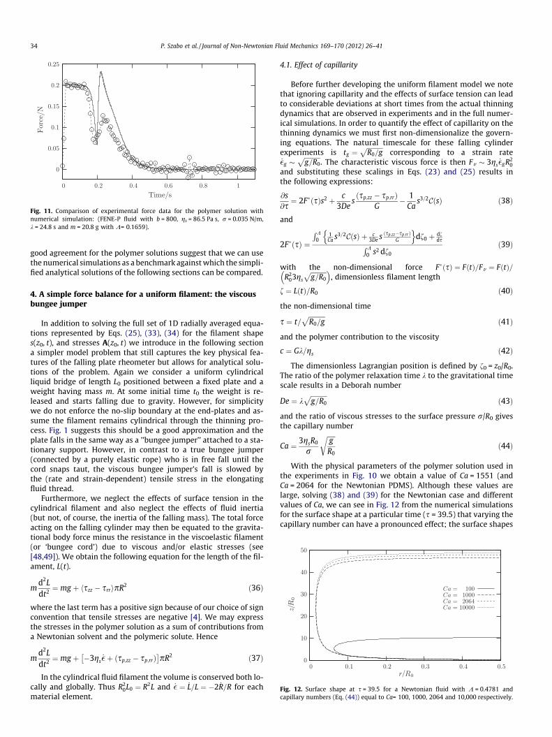
Fig. 11. Comparison of experimental force data for the polymer solution withnumerical simulation: (FENE-P fluid with b = 800, gs = 86.5 Pa s, r = 0.035 N/m,k = 24.8 s and m = 20.8 g with K= 0.1659).

Fig. 12. Surface shape at s = 39.5 for a Newtonian fluid with K = 0.4781 andcapillary numbers (Eq. (44)) equal to Ca= 100, 1000, 2064 and 10,000 respectively.


good agreement for the polymer solutions suggest that we can usethe numerical simulations as a benchmark against which the simpli-fied analytical solutions of the following sections can be compared.

4. A simple force balance for a uniform filament: the viscousbungee jumper

In addition to solving the full set of 1D radially averaged equa-tions represented by Eqs. (25), (33), (34) for the filament shapes(z0, t), and stresses A(z0, t) we introduce in the following sectiona simpler model problem that still captures the key physical fea-tures of the falling plate rheometer but allows for analytical solu-tions of the problem. Again we consider a uniform cylindricalliquid bridge of length L0 positioned between a fixed plate and aweight having mass m. At some initial time t0 the weight is re-leased and starts falling due to gravity. However, for simplicitywe do not enforce the no-slip boundary at the end-plates and as-sume the filament remains cylindrical through the thinning pro-cess. Fig. 1 suggests this should be a good approximation and theplate falls in the same way as a ’’bungee jumper’’ attached to a sta-tionary support. However, in contrast to a true bungee jumper(connected by a purely elastic rope) who is in free fall until thecord snaps taut, the viscous bungee jumper’s fall is slowed bythe (rate and strain-dependent) tensile stress in the elongatingfluid thread.

Furthermore, we neglect the effects of surface tension in thecylindrical filament and also neglect the effects of fluid inertia(but not, of course, the inertia of the falling mass). The total forceacting on the falling cylinder may then be equated to the gravita-tional body force minus the resistance in the viscoelastic filament(or ‘bungee cord’) due to viscous and/or elastic stresses (see[48,49]). We obtain the following equation for the length of the fil-ament, L(t).

md2Ldt2 ¼ mg þ hszz � srripR2 ð36Þ

where the last term has a positive sign because of our choice of signconvention that tensile stresses are negative [4]. We may expressthe stresses in the polymer solution as a sum of contributions froma Newtonian solvent and the polymeric solute. Hence

md2Ldt2 ¼ mg þ �3gs

_�þ ðsp;zz � sp;rrÞ

pR2 ð37Þ

In the cylindrical fluid filament the volume is conserved both lo-cally and globally. Thus R2

0L0 ¼ R2L and _� ¼ _L=L ¼ �2 _R=R for eachmaterial element.

4.1. Effect of capillarity

Before further developing the uniform filament model we notethat ignoring capillarity and the effects of surface tension can leadto considerable deviations at short times from the actual thinningdynamics that are observed in experiments and in the full numer-ical simulations. In order to quantify the effect of capillarity on thethinning dynamics we must first non-dimensionalize the govern-ing equations. The natural timescale for these falling cylinderexperiments is tg ¼

ffiffiffiffiffiffiffiffiffiffiR0=g

pcorresponding to a strain rate

_�g �ffiffiffiffiffiffiffiffiffiffig=R0

p. The characteristic viscous force is then Fv � 3gs

_�gR20

and substituting these scalings in Eqs. (23) and (25) results inthe following expressions:

@s@s¼ 2FðsÞs2 þ c

3Desðsp;zz � sp;rrÞ

G� 1

Cas3=2CðsÞ ð38Þ

and

2FðsÞ ¼

RK0

1Ca s3=2CðsÞ þ c

3De s ðsp;zz�sp;rrÞG

n odf0 þ df

dsRK0 s2 df0

ð39Þ

with the non-dimensional force FðsÞ ¼ FðtÞ=Fv ¼ FðtÞ=R2

03gs


p� �, dimensionless filament length

f ¼ LðtÞ=R0 ð40Þ

the non-dimensional time

s ¼ t=ffiffiffiffiffiffiffiffiffiffiR0=g

pð41Þ

and the polymer contribution to the viscosity

c ¼ Gk=gs ð42Þ

The dimensionless Lagrangian position is defined by f0 = z0/R0.The ratio of the polymer relaxation time k to the gravitational timescale results in a Deborah number

De ¼ kffiffiffiffiffiffiffiffiffiffig=R0

pð43Þ

and the ratio of viscous stresses to the surface pressure r/R0 givesthe capillary number

Ca ¼ 3gsR0

r

ffiffiffiffiffigR0

rð44Þ

With the physical parameters of the polymer solution used inthe experiments in Fig. 10 we obtain a value of Ca = 1551 (andCa = 2064 for the Newtonian PDMS). Although these values arelarge, solving (38) and (39) for the Newtonian case and differentvalues of Ca, we can see in Fig. 12 from the numerical simulationsfor the surface shape at a particular time (s = 39.5) that varying thecapillary number can have a pronounced effect; the surface shapes

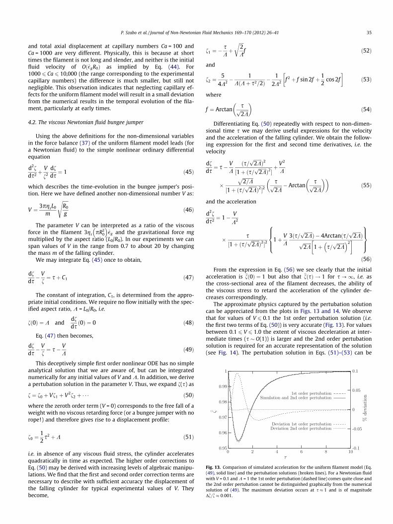
Fig. 13. Comparison of simulated acceleration for the uniform filament model (Eq.(49), solid line) and the pertubation solutions (broken lines). For a Newtonian fluidwith V = 0.1 and K = 1 the 1st order pertubation (dashed line) comes quite close andthe 2nd order pertubation cannot be distinguished graphically from the numericalsolution of (49). The maximum deviation occurs at s 1 and is of magnitudeD€f=€f 0:001.


and total axial displacement at capillary numbers Ca = 100 andCa = 1000 are very different. Physically, this is because at shorttimes the filament is not long and slender, and neither is the initialfluid velocity of Oð _�gR0Þ as implied by Eq. (44). For1000 6 Ca 6 10,000 (the range corresponding to the experimentalcapillary numbers) the difference is much smaller, but still notnegligible. This observation indicates that neglecting capillary ef-fects for the uniform filament model will result in a small deviationfrom the numerical results in the temporal evolution of the fila-ment, particularly at early times.

4.2. The viscous Newtonian fluid bungee jumper

Using the above definitions for the non-dimensional variablesin the force balance (37) of the uniform filament model leads (fora Newtonian fluid) to the simple nonlinear ordinary differentialequation

d2fds2 þ

V

f2

dfds¼ 1 ð45Þ

which describes the time-evolution in the bungee jumper’s posi-tion. Here we have defined another non-dimensional number V as:

V ¼ 3pgsL0

m

ffiffiffiffiffiR0

g

sð46Þ

The parameter V can be interpreted as a ratio of the viscousforce in the filament 3gs pR2

0

� �_�g and the gravitational force mg

multiplied by the aspect ratio (L0/R0). In our experiments we canspan values of V in the range from 0.7 to about 20 by changingthe mass m of the falling cylinder.

We may integrate Eq. (45) once to obtain,

dfds� V

f¼ sþ C1 ð47Þ

The constant of integration, C1, is determined from the appro-priate initial conditions. We require no flow initially with the spec-ified aspect ratio, K = L0/R0, i.e.

fð0Þ ¼ K anddfdsð0Þ ¼ 0 ð48Þ

Eq. (47) then becomes,

dfds� V

f¼ s� V

Kð49Þ

This deceptively simple first order nonlinear ODE has no simpleanalytical solution that we are aware of, but can be integratednumerically for any initial values of V and K. In addition, we derivea pertubation solution in the parameter V. Thus, we expand f(s) as

f ¼ f0 þ Vf1 þ V2f2 þ � � � ð50Þ

where the zeroth order term (V = 0) corresponds to the free fall of aweight with no viscous retarding force (or a bungee jumper with norope!) and therefore gives rise to a displacement profile:

f0 ¼12s2 þK ð51Þ

i.e. in absence of any viscous fluid stress, the cylinder acceleratesquadratically in time as expected. The higher order corrections toEq. (50) may be derived with increasing levels of algebraic manipu-lations. We find that the first and second order correction terms arenecessary to describe with sufficient accuracy the displacement ofthe falling cylinder for typical experimental values of V. Theybecome,

f1 ¼ �sKþ

ffiffiffiffi2K

rf ð52Þ

and

f2 ¼5

4K2 �1

KðKþ s2=2Þ �1

2K2 f 2 þ f sin 2f þ 12

cos 2f �

ð53Þ

where

f ¼ Arctansffiffiffiffiffiffiffi2Kp� �

ð54Þ

Differentiating Eq. (50) repeatedly with respect to non-dimen-sional time s we may derive useful expressions for the velocityand the acceleration of the falling cylinder. We obtain the follow-ing expression for the first and second time derivatives, i.e. thevelocity

dfds¼ s� V

Kðs=

ffiffiffiffiffiffiffi2Kp

Þ2

½1þ ðs=ffiffiffiffiffiffiffi2Kp

Þ2�þ V2

K

�ffiffiffiffiffiffiffiffiffi2=K

p½1þ ðs=


Þ2�2sffiffiffiffiffiffiffi2Kp � Arctan

sffiffiffiffiffiffiffi2Kp� ��

ð55Þ

and the acceleration

d2fds2 ¼ 1� V

K2

� s½1þ ðs=


Þ2�21þ V

K3ðs=


Þ � 4Arctanðs=ffiffiffiffiffiffiffi2Kp

Þffiffiffiffiffiffiffi2Kp

1þ s=ffiffiffiffiffiffiffi2Kp� �2

�8>><>>:

9>>=>>;ð56Þ

From the expression in Eq. (56) we see clearly that the initialacceleration is €fð0Þ ¼ 1 but also that €fðsÞ ! 1 for s ?1, i.e. asthe cross-sectional area of the filament decreases, the ability ofthe viscous stress to retard the acceleration of the cylinder de-creases correspondingly.

The approximate physics captured by the pertubation solutioncan be appreciated from the plots in Figs. 13 and 14. We observethat for values of V 6 0.1 the 1st order pertubation solution (i.e.the first two terms of Eq. (50)) is very accurate (Fig. 13). For valuesbetween 0.1 6 V 6 1.0 the extent of viscous deceleration at inter-mediate times (s � O(1)) is larger and the 2nd order pertubationsolution is required for an accurate representation of the solution(see Fig. 14). The pertubation solution in Eqs. (51)–(53) can be

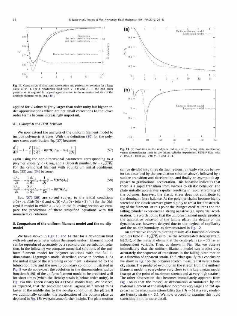
Fig. 14. Comparison of simulated acceleration and pertubation solution for a largevalue of V= 1. For a Newtonian fluid with V = 1.0 and K = 1, the 2nd orderpertubation is required for a good approximation to the numerical solution of theuniform filament model (Eq. (49)).

(a)

(b)

Fig. 15. (a) Evolution in the midplane radius, and (b) falling plate accelerationversus dimensionless time in the falling cylinder experiment. FENE-P fluid withc = 0.52, b = 1000, De = 248, V = 1, and K = 1.


applied for V-values slightly larger than order unity but higher or-der approximations which are not small corrections to the lowerorder terms become increasingly important.

4.3. Oldroyd-B and FENE behavior

We now extend the analysis of the uniform filament model toinclude polymeric stresses. With the definition (30) for the poly-mer stress contribution, Eq. (37) becomes:

d2fds2 ¼ 1� V

f1f

dfdsþ hðtrAÞðAzz � ArrÞ

c3De

�ð57Þ

again using the non-dimensional parameters corresponding to apolymer viscosity, c = Gk/gs, and a Deborah number, De ¼ k


p.

For the cylindrical filament with equilibrium initial conditions,Eqs. (33) and (34) become:

dArr

ds¼ �1

fdfds

Arr þ1

De½1� hðtrAÞArr� ð58Þ

dAzz

ds¼ þ2

fdfds

Azz þ1

De½1� hðtrAÞAzz� ð59Þ

Eqs. (57)–(59) are solved subject to the initial conditionsf(0) = K, df/ds(0) = 0 and Arr(0) = Azz(0) = b/(b + 3) (�1 for the Old-royd-B model in which b ?1). In the following section we com-pare the predictions of these simplified equations with fullnumerical calculations.

5. Comparison of the uniform filament model and the no-slipmodel

We have shown in Figs. 13 and 14 that for a Newtonian fluidwith relevant parameter values the simple uniform filament modelcan be reproduced accurately by a second order pertubation solu-tion. In the following we compare numerical solutions of the uni-form filament model for polymer solutions with the full 1-dimensional Lagrangian model described above in Section 3. Asthe initial stage of the stretching experiment is dominated by thelubrication flow and the no-slip boundary condition illustrated inFig. 8 we do not expect the evolution in the dimensionless radiusfunction R(t)/R0 of the uniform filament model to be predicted wellfor short times (when the Hencky strain is below order unity). InFig. 15a this is seen clearly for a FENE-P model fluid. We observe,as expected, that the one-dimensional Lagrangian filament thinsfaster at the middle due to the no-slip condition at the plates. Ifwe additionally consider the acceleration of the bottom plate asdepicted in Fig. 15b we gain some further insight. The plate motion

can be divided into three distinct regions: an early viscous behav-ior (as described by the pertubation solution above), followed by asudden transition and deceleration, and finally an asymptotic ap-proach to gravitational acceleration. This behavior indicates thatthere is a rapid transition from viscous to elastic behavior. Theplate initially accelerates rapidly, resulting in rapid stretching ofthe polymer; however, the elastic stress does not contribute tothe dominant force balance. As the polymer chains become highlystretched the elastic stresses grow rapidly to resist further stretch-ing of the filament. At this point the ‘bungee cord’ tautens and thefalling cylinder experiences a strong negative (i.e. upwards) accel-eration. It is worth noting that the uniform filament model predictsthe qualitative behavior of the falling plate; the details of thedynamics are, however, delayed due to the neglect of capillarityand the no-slip boundary, as demonstrated in Fig. 12.

An alternative choice to plotting results as a function of dimen-sionless time s ¼ t


pis to use the accumulated Hencky strain,

ln(f/K), of the material element at the centerplane (z0 = 0.5) as anindependent variable. Then, as shown in Fig. 16a, we observeimmediately that the uniform filament model can predict veryaccurately the sequence of transitions in the falling plate motionas a function of apparent strain. To further qualify this conclusionwe show in Fig. 16b the polymer stretch measure trA versus Hen-cky strain. The predicted evolution in the stretch from the uniformfilament model is everywhere very close to the Lagrangian model(except at the point of maximum stretch and at very high strains).The other observation that becomes immediately apparent fromFig. 16b is that the molecular deformation accumulated by thematerial element at the midplane becomes very large and trA ap-proaches the maximum extensibility (i.e. trA ? b) at a very moder-ate Hencky strain � � 3.5. We now proceed to examine this rapidstretching limit in more detail.

(b)

(a)

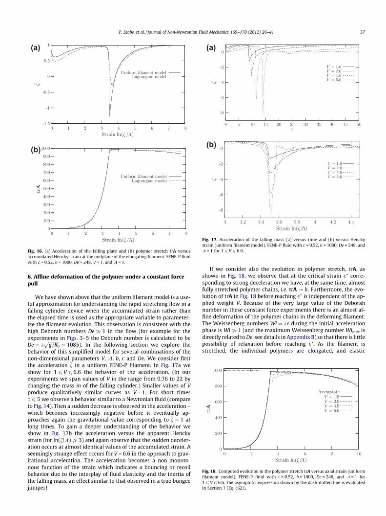
Fig. 16. (a) Acceleration of the falling plate and (b) polymer stretch trA versusaccumulated Hencky strain at the midplane of the elongating filament. FENE-P fluidwith c = 0.52, b = 1000, De = 248, V = 1, and K = 1.

(a)

(b)

Fig. 17. Acceleration of the falling mass (a) versus time and (b) versus Henckystrain (uniform filament model). FENE-P fluid with c = 0.52, b = 1000, De = 248, andK = 1 for 1 6 V 6 6.6.

Fig. 18. Computed evolution in the polymer stretch trA versus axial strain (uniformfilament model). FENE-P fluid with c = 0.52, b = 1000, De = 248, and K = 1 for1 6 V 6 6.6. The asymptotic expression shown by the dash-dotted line is evaluatedin Section 7 (Eq. (62)).


6. Affine deformation of the polymer under a constant forcepull

We have shown above that the uniform filament model is a use-ful approximation for understanding the rapid stretching flow in afalling cylinder device when the accumulated strain rather thanthe elapsed time is used as the appropriate variable to parameter-ize the filament evolution. This observation is consistent with thehigh Deborah numbers De� 1 in the flow (for example for theexperiments in Figs. 3–5 the Deborah number is calculated to beDe ¼ k


p¼ 1085). In the following section we explore the

behavior of this simplified model for several combinations of thenon-dimensional parameters V, K, b, c and De. We consider firstthe acceleration €f in a uniform FENE-P filament. In Fig. 17a weshow for 1 6 V 6 6.6 the behavior of the acceleration. (In ourexperiments we span values of V in the range from 0.76 to 22 bychanging the mass m of the falling cylinder.) Smaller values of Vproduce qualitatively similar curves as V = 1. For short timess 6 5 we observe a behavior similar to a Newtonian fluid (compareto Fig. 14). Then a sudden decrease is observed in the acceleration –which becomes increasingly negative before it eventually ap-proaches again the gravitational value corresponding to €f ¼ 1 atlong times. To gain a deeper understanding of the behavior weshow in Fig. 17b the acceleration versus the apparent Henckystrain (for ln(f/K) P 3) and again observe that the sudden deceler-ation occurs at almost identical values of the accumulated strain. Aseemingly strange effect occurs for V = 6.6 in the approach to grav-itational acceleration. The acceleration becomes a non-monoto-nous function of the strain which indicates a bouncing or recoilbehavior due to the interplay of fluid elasticity and the inertia ofthe falling mass, an effect similar to that observed in a true bungeejumper!

If we consider also the evolution in polymer stretch, trA, asshown in Fig. 18, we observe that at the critical strain �⁄ corre-sponding to strong deceleration we have, at the same time, almostfully stretched polymer chains, i.e. trA ? b. Furthermore, the evo-lution of trA in Fig. 18 before reaching �⁄ is independent of the ap-plied weight V. Because of the very large value of the Deborahnumber in these constant force experiments there is an almost af-fine deformation of the polymer chains in the deforming filament.The Weissenberg numbers Wi ¼ k _� during the initial accelerationphase is Wi� 1 (and the maximum Weissenberg number Wimax isdirectly related to De, see details in Appendix B) so that there is littlepossibility of relaxation before reaching �⁄. As the filament isstretched, the individual polymers are elongated, and elastic


stresses build up in the filament. As the chains reach full elonga-tion and snap taut the falling motion is rapidly arrested and thefalling cylinder stops or even starts to bounce depending on thechoice of parameters. A similar observation was made by Keiller[19] who studied a falling drop of an Oldroyd-B fluid.

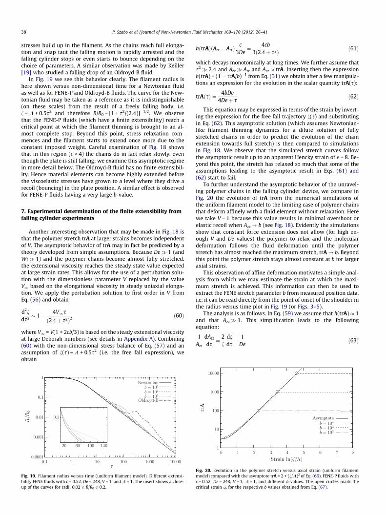
In Fig. 19 we see this behavior clearly. The filament radius ishere shown versus non-dimensional time for a Newtonian fluidas well as for FENE-P and Oldroyd-B fluids. The curve for the New-tonian fluid may be taken as a reference as it is indistinguishable(on these scales) from the result of a freely falling body, i.e.f = K + 0.5s2 and therefore R/R0 = [1 + s2/(2K)]�1/2. We observethat the FENE-P fluids (which have a finite extensibility) reach acritical point at which the filament thinning is brought to an al-most complete stop. Beyond this point, stress relaxation com-mences and the filament starts to extend once more due to theconstant imposed weight. Careful examination of Fig. 18 showsthat in this region (� > 4) the chains do in fact relax slowly, eventhough the plate is still falling; we examine this asymptotic regimein more detail below. The Oldroyd-B fluid has no finite extensibil-ity. Hence material elements can become highly extended beforethe viscoelastic stresses have grown to a level where they drive arecoil (bouncing) in the plate position. A similar effect is observedfor FENE-P fluids having a very large b-value.

7. Experimental determination of the finite extensibility fromfalling cylinder experiments

Another interesting observation that may be made in Fig. 18 isthat the polymer stretch trA at larger strains becomes independentof V. The asymptotic behavior of trA may in fact be predicted by atheory developed from simple assumptions. Because De� 1 (andWi� 1) and the polymer chains become almost fully stretched,the extensional viscosity reaches the steady state value expectedat large strain rates. This allows for the use of a pertubation solu-tion with the dimensionless parameter V replaced by the valueV1 based on the elongational viscosity in steady uniaxial elonga-tion. We apply the pertubation solution to first order in V fromEq. (56) and obtain

d2fds2 � 1� 4V1s

ð2Kþ s2Þ2ð60Þ

where V1 = V(1 + 2cb/3) is based on the steady extensional viscosityat large Deborah numbers (see details in Appendix A). Combining(60) with the non-dimensional stress balance of Eq. (57) and anassumption of f(s) = K + 0.5s2 (i.e. the free fall expression), weobtain

Fig. 19. Filament radius versus time (uniform filament model). Different extensi-bility FENE fluids with c = 0.52, De = 248, V = 1, and K = 1. The insert shows a close-up of the curves for radii 0.02 6 R/R0 6 0.2.

hðtrAÞðAzz � ArrÞc

3De¼ 4cb

3ð2Kþ s2Þ ð61Þ

which decays monotonically at long times. We further assume thats2� 2K and Azz� Arr and Azz trA. Inserting then the expressionh(trA) = (1 � trA/b)�1 from Eq. (31) we obtain after a few manipula-tions an expression for the evolution in the scalar quantity trA(s):

trAðsÞ ¼ 4bDe4Deþ s

ð62Þ

This equation may be expressed in terms of the strain by invert-ing the expression for the free fall trajectory f(s) and substitutingin Eq. (62). This asymptotic solution (which assumes Newtonian-like filament thinning dynamics for a dilute solution of fullystretched chains in order to predict the evolution of the chainextension towards full stretch) is then compared to simulationsin Fig. 18. We observe that the simulated stretch curves followthe asymptotic result up to an apparent Hencky strain of � = 8. Be-yond this point, the stretch has relaxed so much that some of theassumptions leading to the asymptotic result in Eqs. (61) and(62) start to fail.

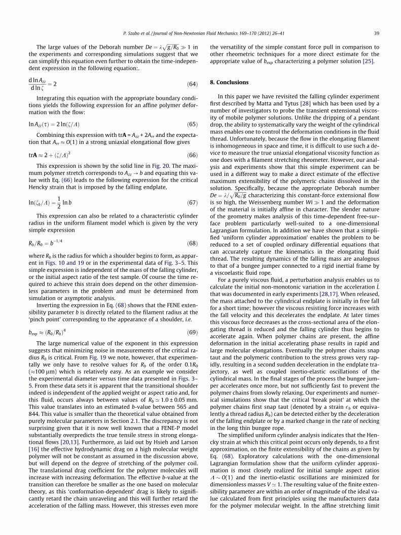
To further understand the asymptotic behavior of the unravel-ing polymer chains in the falling cylinder device, we compare inFig. 20 the evolution of trA from the numerical simulations ofthe uniform filament model to the limiting case of polymer chainsthat deform affinely with a fluid element without relaxation. Herewe take V = 1 because this value results in minimal overshoot orelastic recoil when Azz ? b (see Fig. 18). Evidently the simulationsshow that constant force extension does not allow (for high en-ough V and De values) the polymer to relax and the moleculardeformation follows the fluid deformation until the polymerstretch has almost reached the maximum stretch, trA ? b. Beyondthis point the polymer stretch stays almost constant at b for largeraxial strains.

This observation of affine deformation motivates a simple anal-ysis from which we may estimate the strain at which the maxi-mum stretch is achieved. This information can then be used toextract the FENE stretch parameter b from measured position data,i.e. it can be read directly from the point of onset of the shoulder inthe radius versus time plot in Fig. 19 (or Figs. 3–5).

The analysis is as follows. In Eq. (59) we assume that h(trA) 1and that Azz� 1. This simplification leads to the followingequation:

1Azz

dAzz

ds¼ 2

fdfds� 1

Deð63Þ

Fig. 20. Evolution in the polymer stretch versus axial strain (uniform filamentmodel) compared with the asymptote trA = 2 + (f/K)2 of Eq. (66). FENE-P fluids withc = 0.52, De = 248, V = 1, K = 1, and different b-values. The open circles mark thecritical strain fb for the respective b values obtained from Eq. (67).


The large values of the Deborah number De ¼ kffiffiffiffiffiffiffiffiffiffig=R0

p� 1 in

the experiments and corresponding simulations suggest that wecan simplify this equation even further to obtain the time-indepen-dent expression in the following equation:.

d ln Azz

d ln f¼ 2 ð64Þ

Integrating this equation with the appropriate boundary condi-tions yields the following expression for an affine polymer defor-mation with the flow:

ln AzzðsÞ ¼ 2 lnðf=KÞ ð65Þ

Combining this expression with trA = Azz + 2Arr and the expecta-tion that Arr O(1) in a strong uniaxial elongational flow gives

trA 2þ ðf=KÞ2 ð66Þ

This expression is shown by the solid line in Fig. 20. The maxi-mum polymer stretch corresponds to Azz ? b and equating this va-lue with Eq. (66) leads to the following expression for the criticalHencky strain that is imposed by the falling endplate,

lnðfb=KÞ ¼12

ln b ð67Þ

This expression can also be related to a characteristic cylinderradius in the uniform filament model which is given by the verysimple expression

Rb=R0 ¼ b�1=4 ð68Þ

where Rb is the radius for which a shoulder begins to form, as appar-ent in Figs. 10 and 19 or in the experimental data of Fig. 3–5. Thissimple expression is independent of the mass of the falling cylinder,or the initial aspect ratio of the test sample. Of course the time re-quired to achieve this strain does depend on the other dimension-less parameters in the problem and must be determined fromsimulation or asymptotic analysis.

Inverting the expression in Eq. (68) shows that the FENE exten-sibility parameter b is directly related to the filament radius at the‘pinch point’ corresponding to the appearance of a shoulder, i.e.

bexp ðR0=RbÞ4 ð69Þ

The large numerical value of the exponent in this expressionsuggests that minimizing noise in measurements of the critical ra-dius Rb is critical. From Fig. 19 we note, however, that experimen-tally we only have to resolve values for Rb of the order 0.1R0

(100 lm) which is relatively easy. As an example we considerthe experimental diameter versus time data presented in Figs. 3–5. From these data sets it is apparent that the transitional shoulderindeed is independent of the applied weight or aspect ratio and, forthis fluid, occurs always between values of Rb ’ 1.0 ± 0.05 mm.This value translates into an estimated b-value between 565 and844. This value is smaller than the theoretical value obtained frompurely molecular parameters in Section 2.1. The discrepancy is notsurprising given that it is now well known that a FENE-P modelsubstantially overpredicts the true tensile stress in strong elonga-tional flows [20,13]. Furthermore, as laid out by Hsieh and Larson[16] the effective hydrodynamic drag on a high molecular weightpolymer will not be constant as assumed in the discussion above,but will depend on the degree of stretching of the polymer coil.The translational drag coefficient for the polymer molecules willincrease with increasing deformation. The effective b-value at thetransition can therefore be smaller as the one based on moleculartheory, as this ‘conformation-dependent’ drag is likely to signifi-cantly retard the chain unraveling and this will further retard theacceleration of the falling mass. However, this stresses even more

the versatility of the simple constant force pull in comparison toother rheometric techniques for a more direct estimate for theappropriate value of bexp characterizing a polymer solution [25].

8. Conclusions

In this paper we have revisited the falling cylinder experimentfirst described by Matta and Tytus [28] which has been used by anumber of investigators to probe the transient extensional viscos-ity of mobile polymer solutions. Unlike the dripping of a pendantdrop, the ability to systematically vary the weight of the cylindricalmass enables one to control the deformation conditions in the fluidthread. Unfortunately, because the flow in the elongating filamentis inhomogeneous in space and time, it is difficult to use such a de-vice to measure the true uniaxial elongational viscosity function asone does with a filament stretching rheometer. However, our anal-ysis and experiments show that this simple experiment can beused in a different way to make a direct estimate of the effectivemaximum extensibility of the polymeric chains dissolved in thesolution. Specifically, because the appropriate Deborah numberDe ¼ k=

ffiffiffiffiffiffiffiffiffiffiR0=g

pcharacterizing this constant-force extensional flow

is so high, the Weissenberg number Wi� 1 and the deformationof the material is initially affine in character. The slender natureof the geometry makes analysis of this time-dependent free-sur-face problem particularly well-suited to a one-dimensionalLagrangian formulation. In addition we have shown that a simpli-fied ‘uniform cylinder approximation’ enables the problem to bereduced to a set of coupled ordinary differential equations thatcan accurately capture the kinematics in the elongating fluidthread. The resulting dynamics of the falling mass are analogousto that of a bungee jumper connected to a rigid inertial frame bya viscoelastic fluid rope.

For a purely viscous fluid, a perturbation analysis enables us tocalculate the initial non-monotonic variation in the acceleration €Lthat was documented in early experiments [28,17]. When released,the mass attached to the cylindrical endplate is initially in free fallfor a short time; however the viscous resisting force increases withthe fall velocity and this decelerates the endplate. At later timesthis viscous force decreases as the cross-sectional area of the elon-gating thread is reduced and the falling cylinder thus begins toaccelerate again. When polymer chains are present, the affinedeformation in the initial accelerating phase results in rapid andlarge molecular elongations. Eventually the polymer chains snaptaut and the polymeric contribution to the stress grows very rap-idly, resulting in a second sudden deceleration in the endplate tra-jectory, as well as coupled inertio-elastic oscillations of thecylindrical mass. In the final stages of the process the bungee jum-per accelerates once more, but not sufficiently fast to prevent thepolymer chains from slowly relaxing. Our experiments and numer-ical simulations show that the critical ‘break point’ at which thepolymer chains first snap taut (denoted by a strain �b or equiva-lently a thread radius Rb) can be detected either by the decelerationof the falling endplate or by a marked change in the rate of neckingin the long thin bungee rope.

The simplified uniform cylinder analysis indicates that the Hen-cky strain at which this critical point occurs only depends, to a firstapproximation, on the finite extensibility of the chains as given byEq. (68). Exploratory calculations with the one-dimensionalLagrangian formulation show that the uniform cylinder approxi-mation is most closely realized for initial sample aspect ratiosK � O(1) and the inertio-elastic oscillations are minimized fordimensionless masses V ’ 1. The resulting value of the finite exten-sibility parameter are within an order of magnitude of the ideal va-lue calculated from first principles using the manufacturers datafor the polymer molecular weight. In the affine stretching limit


that is consistent with this constant tensile force device, the totalHencky strain required to achieve maximum molecular stretchonly depends on the 1/4th power of the extensibility parameter.The resulting strains are thus surprisingly moderate, correspond-ing to radius reductions of only factors of 10–30. They are thereforerelatively easy to observe, provided a high speed imaging system isavailable and a reliable mechanism is developed for cleanly releas-ing the lower plate and attached cylindrical weight (in our experi-ence this is not trivial to achieve). The falling cylinder device maythus serve a useful role for quickly establishing constitutive param-eters relevant to low viscosity polymer solutions at large deforma-tion rates and large strains.

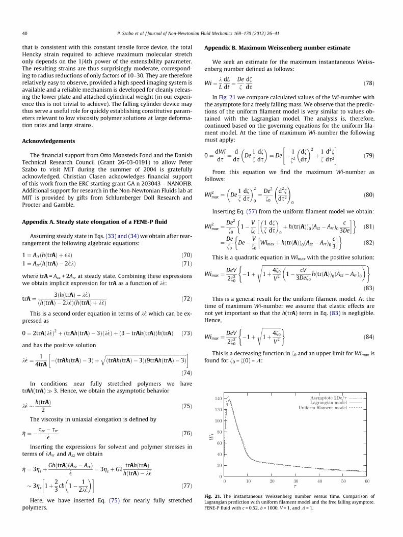
Acknowledgements

The financial support from Otto Mønsteds Fond and the DanishTechnical Research Council (Grant 26-03-0191) to allow PeterSzabo to visit MIT during the summer of 2004 is gratefullyacknowledged. Christian Clasen acknowledges financial supportof this work from the ERC starting grant GA n 203043 – NANOFIB.Additional support for research in the Non-Newtonian Fluids lab atMIT is provided by gifts from Schlumberger Doll Research andProcter and Gamble.

Fig. 21. The instantaneous Weissenberg number versus time. Comparison ofLagrangian prediction with uniform filament model and the free falling asymptote.FENE-P fluid with c = 0.52, b = 1000, V = 1, and K = 1.

Appendix A. Steady state elongation of a FENE-P fluid

Assuming steady state in Eqs. (33) and (34) we obtain after rear-rangement the following algebraic equations:

1 ¼ ArrðhðtrAÞ þ _�kÞ ð70Þ1 ¼ AzzðhðtrAÞ � 2 _�kÞ ð71Þ

where trA = Azz + 2Arr at steady state. Combining these expressionswe obtain implicit expression for trA as a function of k _�:

trA ¼ 3ðhðtrAÞ � k _�ÞðhðtrAÞ � 2k _�ÞðhðtrAÞ þ k _�Þ ð72Þ

This is a second order equation in terms of k _� which can be ex-pressed as

0 ¼ 2trAðk _�Þ2 þ ðtrAhðtrAÞ � 3Þðk _�Þ þ ð3� trAhðtrAÞÞhðtrAÞ ð73Þ

and has the positive solution

k _� ¼ 14trA

�ðtrAhðtrAÞ � 3Þ þffiffiffiffiffiffiffiffiffiffiffiffiffiffiffiffiffiffiffiffiffiffiffiffiffiffiffiffiffiffiffiffiffiffiffiffiffiffiffiffiffiffiffiffiffiffiffiffiffiffiffiffiffiffiffiffiffiffiffiffiffiffiffiffiffiffiffiffiffiðtrAhðtrAÞ � 3Þð9trAhðtrAÞ � 3Þ

q �ð74Þ

In conditions near fully stretched polymers we havetrAh(trA)� 3. Hence, we obtain the asymptotic behavior

k _� � hðtrAÞ2

ð75Þ

The viscosity in uniaxial elongation is defined by

�g ¼ � szz � srr

_�ð76Þ

Inserting the expressions for solvent and polymer stresses interms of _�Arr and Azz we obtain

�g ¼ 3gs þGhðtrAÞðAzz � ArrÞ

_�¼ 3gs þ Gk

trAhðtrAÞhðtrAÞ � k _�

� 3gs 1þ 23

cb 1� 12k _�

� � �ð77Þ

Here, we have inserted Eq. (75) for nearly fully stretchedpolymers.

Appendix B. Maximum Weissenberg number estimate

We seek an estimate for the maximum instantaneous Weiss-enberg number defined as follows:

Wi ¼ kL

dLdt¼ De

fdfds

ð78Þ

In Fig. 21 we compare calculated values of the Wi-number withthe asymptote for a freely falling mass. We observe that the predic-tions of the uniform filament model is very similar to values ob-tained with the Lagrangian model. The analysis is, therefore,continued based on the governing equations for the uniform fila-ment model. At the time of maximum Wi-number the followingmust apply:

0 ¼ dWids¼ d

dsDe

1f

dfds

� �¼ De � 1

f2

dfds

� �2

þ 1f

d2fds2

" #ð79Þ

From this equation we find the maximum Wi-number asfollows:

Wi2max ¼ De

1f

dfds

� �2

0¼ De2

f0

d2fds2

!0

ð80Þ

Inserting Eq. (57) from the uniform filament model we obtain:

Wi2max ¼

De2

f01� V

f0

1f

dfds

� �0þ hðtrðAÞÞ0ðAzz � ArrÞ0

c3De

�� ð81Þ

¼ Def0

De� Vf0

Wimax þ hðtrðAÞÞ0ðAzz � ArrÞ0c3

h i� �ð82Þ

This is a quadratic equation in Wimax with the positive solution:

Wimax ¼DeV

2f20

�1þ

ffiffiffiffiffiffiffiffiffiffiffiffiffiffiffiffiffiffiffiffiffiffiffiffiffiffiffiffiffiffiffiffiffiffiffiffiffiffiffiffiffiffiffiffiffiffiffiffiffiffiffiffiffiffiffiffiffiffiffiffiffiffiffiffiffiffiffiffiffiffiffiffiffiffiffiffiffiffiffiffiffiffiffiffiffiffiffiffi1þ 4f0

V2 1� cV3Def0

hðtrðAÞÞ0ðAzz � ArrÞ0� �s( )

ð83Þ

This is a general result for the uniform filament model. At thetime of maximum Wi-number we assume that elastic effects arenot yet important so that the h(trA) term in Eq. (83) is negligible.Hence,

Wimax ¼DeV

2f20

�1þ

ffiffiffiffiffiffiffiffiffiffiffiffiffiffiffiffi1þ 4f0

V2

s( )ð84Þ

This is a decreasing function in f0 and an upper limit for Wimax isfound for f0 = f(0) = K:


Wimax ¼DeV

2K2 �1þ

ffiffiffiffiffiffiffiffiffiffiffiffiffiffiffiffi1þ 4K

V2

s( )ð85Þ

Furthermore, we note that as V ? 0 we haveWimax ! De=f3=2

0 6 De=K3=2.

References

[1] S.L. Anna, G.H. McKinley, Elasto-capillary thinning and breakup of modelelastic liquids, J. Rheol. 45 (2001) 115–138.

[2] S.L. Anna, G.H. McKinley, D.A. Nguyen, T. Sridhar, S.J. Muller, J. Huang, D.F.James, An interlaboratory comparison of measurements from filament-stretching rheometers using common test fluids, J. Rheol. 45 (2001) 83–114.

[3] A. Bach, H.K. Rasmussen, O. Hassager, Extensional viscosity for polymer meltsmeasured in the filament stretching rheometer, J. Rheol. 47 (2003) 429–441.

[4] R.B. Bird, R.C. Armstrong, O. Hassager, Dynamics of Polymeric Liquids, FluidMechanics, second ed., vol. 1, John Wiley & Sons, New York, 1987.

[5] H. Chang, A.S. Lodge, A possible mechanism for stabilizing elongational flow incertain polymeric liquids at constant temperature and composition, Rheol.Acta 10 (1971) 448–449.

[6] L. Campo-Deano, C. Clasen, The slow retraction method (SRM) for thedetermination of ultra-short relaxation times in capillary breakupexperiments, J. Non-Newton. Fluid Mech. 165 (2010) 1688–1699.

[7] C. Clasen, Capillary breakup extensional rheometry of semi-dilute polymersolutions, Korea–Australia Rheol. J. 22 (2010) 331–338.

[8] C. Clasen, J. Bico, V.M. Entov, G.H. McKinley, ’Gobbling drops’: the jetting–dripping transition in flows of polymer solutions, J. Fluid Mech. 636 (2009) 5–40.

[9] C. Clasen, J. Eggers, M.A. Fontelos, J. Li, G.H. McKinley, The beads-on-stringstructure of viscoelastic threads, J. Fluid Mech. 556 (2006) 283–308.

[10] C. Clasen, J.P. Plog, W.M. Kulicke, M. Owens, C. Macosko, L.E. Scriven, M. Verani,G.H. McKinley, How dilute are dilute solutions in extensional flows?, J Rheol.50 (2006) 849–881.

[11] J. Eggers, Nonlinear dynamics and breakup of free-surface flows, Rev. Mod.Phys. 69 (1997) 865–929.

[12] V.M. Entov, E.J. Hinch, Effect of a spectrum of relaxation times on the capillarythinning of a filament of elastic liquid, J. Non-Newton. Fluid Mech. 72 (1997)31–53.

[13] I. Ghosh, G.H. McKinley, R.A. Brown, R.C. Armstrong, Deficiencies of FENEdumbbell models in describing the rapid stretching of dilute polymersolutions, J. Rheol. 45 (2001) 721–758.

[14] O.G. Harlen, J.M. Rallison, P. Szabo, A split Lagrangian–Eulerian method forsimulating transient viscoelastic flows, J. Non-Newton. Fluid Mech. 60 (1995)81–104.

[15] O. Hassager, J.M.R. Marin, K.J. Yu, H.K. Rasmussen, Polymeric liquids inextension: fluid mechanics or rheometry?, Rheol Acta 49 (2010) 543–554.

[16] C.C. Hsieh, R. Larson, Prediction of coil–stretch hysteresis for dilutepolystyrene molecules in extensional flow, J. Rheol. 49 (2005) 1081–1089.

[17] W.M. Jones, N.E. Hudson, J. Ferguson, The extensional properties of M1obtained from the stretching of a filament by a falling pendant drop, J. Non-Newton. Fluid Mech. 35 (1990) 263–276.

[18] W.M. Jones, I.J. Rees, The stringiness of dilute polymer solutions, J. Non-Newton. Fluid Mech. 11 (1982) 257–268.

[19] R.A. Keiller, Extending filaments of an Oldroyd-B fluid, J. Non-Newton. FluidMech. 42 (1992) 37–48.

[20] R. Keunings, On the Peterlin approximation for finitely extensible dumbbells, J.Non-Newton. Fluid Mech. 68 (1997) 85–100.

[21] M.I. Kolte, P. Szabo, Capillary thinning of polymeric filaments, J. Rheol. 43(1999) 609–625.

[22] L.D. Landau, E.M. Lifshitz, Fluid Mechanics, Pergamon, Oxford, 1987.[23] L. Li, R.G. Larson, T. Sridhar, Brownian dynamics simulations of dilute

polystyrene solutions, J. Rheol. 44 (2000) 291–322.[24] R.F. Liang, M.R. Mackley, Rheological characterization of the time and strain

dependence for polyisobutylene solutions, J. Non-Newton. Fluid Mech. 52(1994) 387–405.

[25] A. Lindner, J. Vermant, D. Bonn, How to obtain the elongational viscosity ofdilute polymer solutions?, Phys A – Stat. Mech. Appl. 319 (2003) 125–133.

[26] M.E. Mackay, D.V. Boger, An explanation of the rheological properties of Bogerfluids, J. Non-Newton. Fluid Mech. 22 (1987) 235–243.

[27] J.M.R. Marin, H.K. Rasmussen, Lagrangian finite-element method for thesimulation of K-BKZ fluids with third order accuracy, J. Non-Newton. FluidMech. 156 (2009) 177–188.

[28] J.E. Matta, R.P. Tytus, Liquid stretching using a falling cylinder, J. Non-Newton.Fluid Mech. 35 (1990) 215–229.

[29] G.H. McKinley, T. Sridhar, Filament-stretching rheometry of complex fluids,Ann. Rev. Fluid Mech. 34 (2002) 375–415.

[30] G.H. McKinley, A. Tripathi, How to extract the Newtonian viscosity fromcapillary breakup measurements in a filament rheometer, J. Rheol. 44 (2000)653–670.

[31] E. Miller, C. Clasen, J.P. Rothstein, The effect of step-stretch parameters oncapillary breakup extensional rheology (CaBER) measurements, Rheol. Acta 48(2009) 625–639.

[32] J. Meissner, Experimental aspects in polymer melt elongational rheometry,Chem. Eng. Commun. 33 (1985) 159–180.

[33] N. Morrison, J.M. Rallison, Transient 3D-flow of polymer solutions: aLagrangian computational method, J. Non-Newton. Fluid Mech. 165 (2010)1241–1257.

[34] H. Münstedt, New universal extensional rheometer for polymer melts –measurements on a polystyrene sample, J. Rheol. 23 (1979) 421–436.

[35] H. Münstedt, S. Kurzbeck, L. Egersdörfer, Influence of molecular structure onrheological properties of polyethylenes. II. Elongational behavior, Rheol. Acta37 (1998) 21–29.

[36] J.P. Plog, W.M. Kulicke, C. Clasen, Influence of the molar mass distribution onthe elongational behaviour of polymer solutions in capillary breakup, Appl.Rheol. 15 (2005) 28–37.

[37] H.K. Rasmussen, Time-dependent finite-element method for the simulation ofthree-dimensional viscoelastic flow with integral models, J. Non-Newton.Fluid Mech. 84 (1999) 217–232.

[38] H.K. Rasmussen, O. Hassager, Simulation of transient viscoelastic flow withsecond order time integration, J. Non-Newton. Fluid Mech. 56 (1995) 65–84.

[39] M. Renardy, Some comments on the surface-tension driven break-up (or thelack of it) of viscoelastic jets, J. Non-Newton. Fluid Mech. 51 (1994) 97–107.

[40] M. Renardy, A numerical study of the asymptotic evolution and breakup ofNewtonian and viscoelastic jets, J. Non-Newton. Fluid Mech. 59 (1995) 267–282.

[41] M. Sentmanat, B.N. Wang, G.H. McKinley, Measuring the transient extensionalrheology of polyethylene melts using the SER universal testing platform, J.Rheol. 49 (2005) 585–606.

[42] L.B. Smolka, A. Belmonte, Drop pinch-off and filament dynamics of wormlikemicellar fluids, J. Non-Newton. Fluid Mech. 115 (2003) 1–25.

[43] L.B. Smolka, A. Belmonte, D.M. Henderson, T.P. Witelski, Exact solution for theextensional flow of a viscoelastic filament, Eur. J. Appl. Math.matics 15 (2004)679–712.

[44] S.H. Spiegelberg, D.C. Ables, G.H. McKinley, The role of end-effects onmeasurements of extensional viscosity in filament stretching rheometers, J.Non-Newton. Fluid Mech. 64 (1996) 229–267.

[45] T. Sridhar, V. Tirtaatmadja, D.A. Nguyen, R.K. Gupta, Measurement ofextensional viscosity of polymer solutions, J. Non-Newton. Fluid Mech. 40(1991) 271–280.

[46] M. Stelter, G. Brenn, Validation and application of a novel elongational devicefor polymer solutions, J. Rheol. 44 (2000) 595–616.

[47] Y.M. Stokes, E.O. Tuck, L.W. Schwartz, Extensional fall of a very viscous fluiddrop, Quart. J. Mech. Appl. Math. 53 (2000) 565–582.

[48] P. Szabo, Transient filament stretching rheometer. I: Force balance analysis,Rheol. Acta 36 (1997) 277–284.

[49] P. Szabo, G.H. McKinley, Filament stretching rheometer: inertia compensationrevisited, Rheol. Acta 42 (2003) 269–272.

[50] M. Yao, G.H. McKinley, Numerical simulation of extensional deformations ofviscoelastic liquid bridges in filament stretching devices, J. Non-Newton. FluidMech. 74 (1998) 47–88.

[51] M. Yao, G.H. McKinley, B. Debbaut, Extensional deformation, stress relaxationand necking failure of viscoelastic filaments, J. Non-Newton. Fluid Mech. 79(1998) 469–501.

Documents

Constant force extensional rheometry of polymer solutions