Constant Density Spanners for Wireless Ad hoc Networks

Kishore Kothapalli (JHU)Melih Onus (ASU)Christian Scheideler (JHU)Andrea Richa (ASU)

1

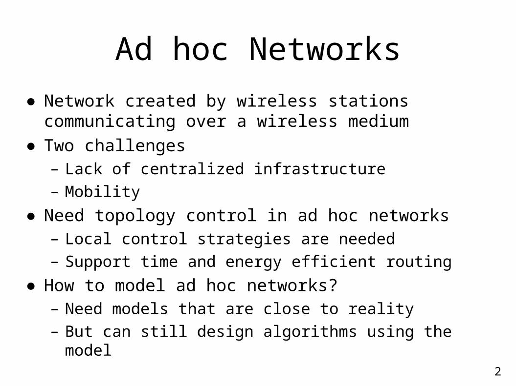
Ad hoc Networks

● Network created by wireless stations communicating over a wireless medium

● Two challenges– Lack of centralized infrastructure– Mobility

2

Ad hoc Networks

● Network created by wireless stations communicating over a wireless medium

● Two challenges– Lack of centralized infrastructure

– Mobility

● Need topology control in ad hoc networks– Local control strategies are needed

– Support time and energy efficient routing

● How to model ad hoc networks?– Need models that are close to reality

– But can still design algorithms using the model2

Modeling Wireless Networks

● Wireless communication very difficult to model accurately– Shape of transmission range

– Interference

– Mobility

– Physical Carrier Sensing

3

Outline Introduction

→Models of Wireless networks

● Our model

● Our results

● Problem description

– Running Example

● Conclusions

4

Models of Wireless Networks

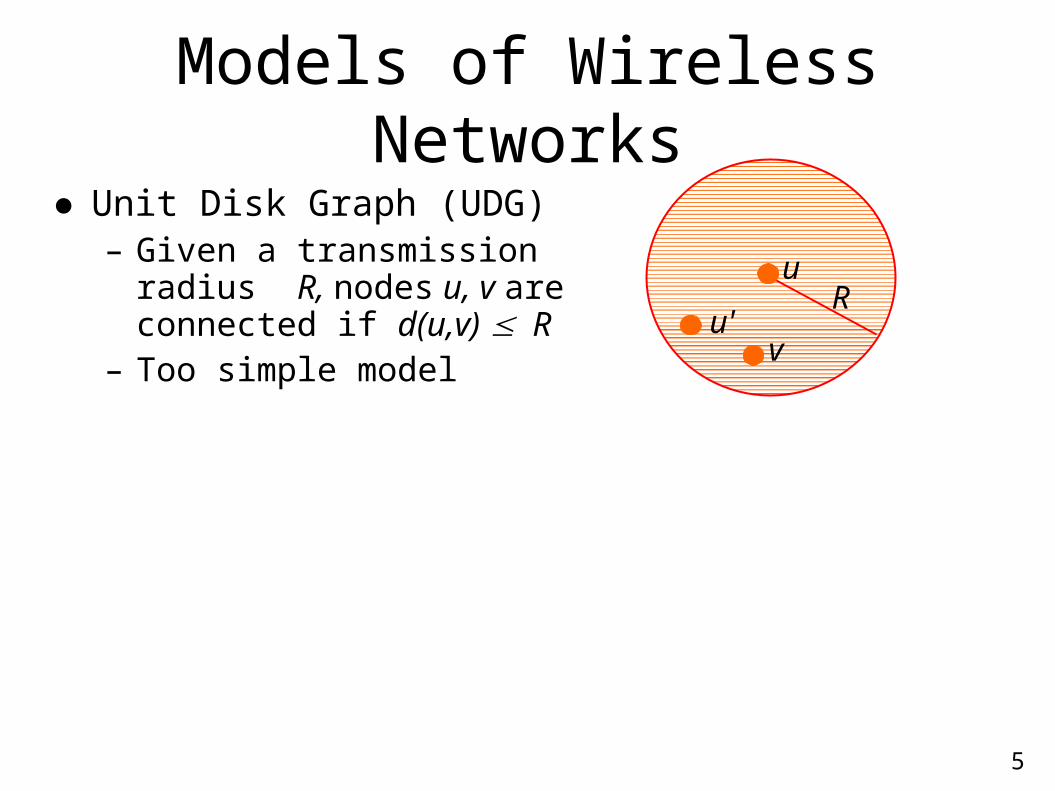
● Unit Disk Graph (UDG)– Given a transmission radius

R, nodes u, v are connected if d(u,v) ≤ R

– Too simple model

5

uR

vu'

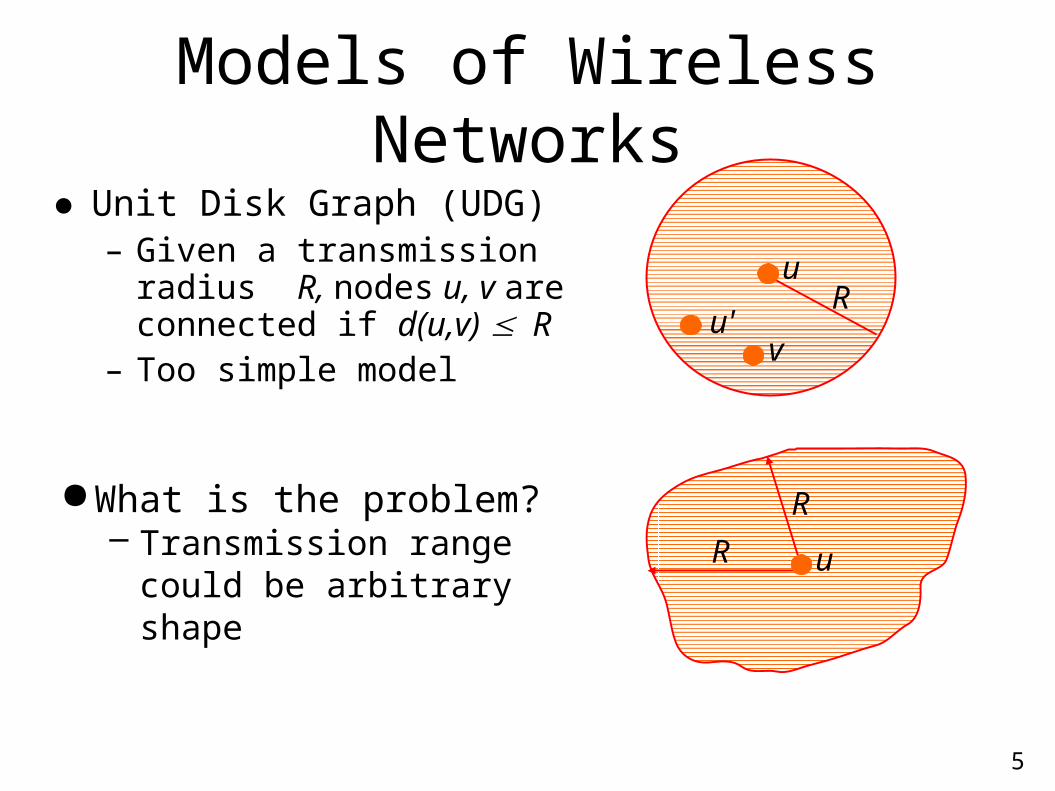
●What is the problem?– Transmission range could be

arbitrary shape

5

R

R

uR

vu'

u

Models of Wireless Networks

● Unit Disk Graph (UDG)– Given a transmission radius

R, nodes u, v are connected if d(u,v) ≤ R

– Too simple model

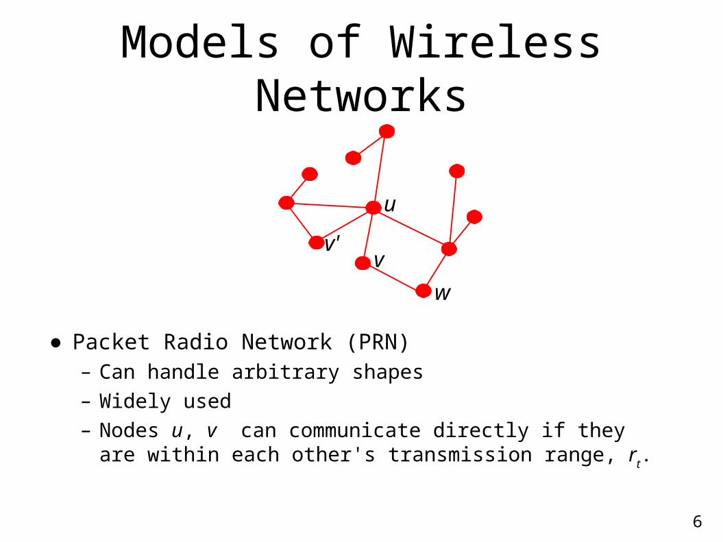
● Packet Radio Network (PRN)– Can handle arbitrary shapes

– Widely used

– Nodes u, v can communicate directly if they are within each other's transmission range, rt.

6

u

v

w

v'

Models of Wireless Networks

What is the problem?

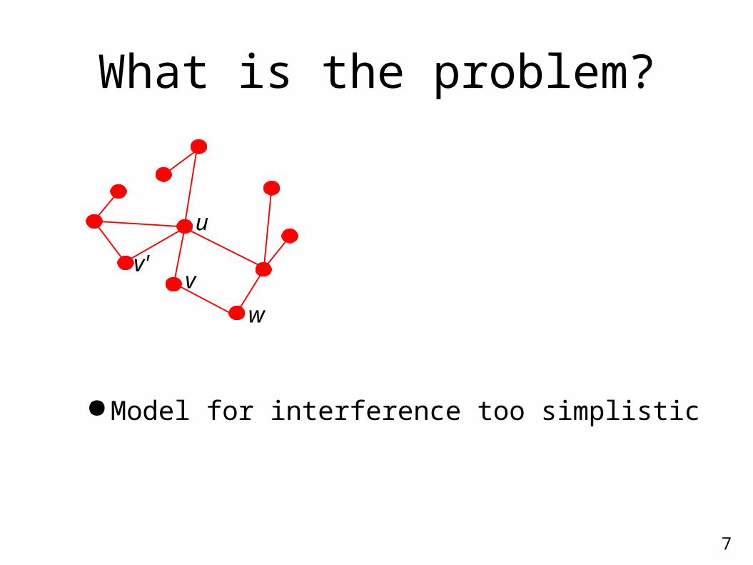
●Model for interference too simplistic

7

u

v

w

v'

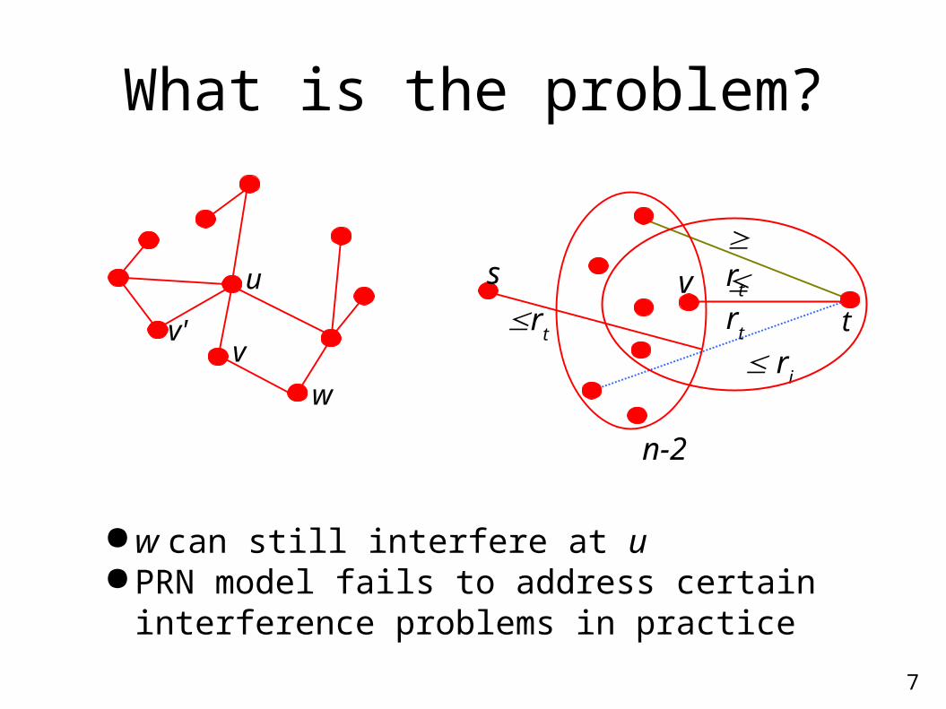
●w can still interfere at u●PRN model fails to address certain interference

problems in practice

v

n-2

s

t ≤rt

≤ rt

≤ ri

≥ rt

7

What is the problem?

u

v

w

v'

8

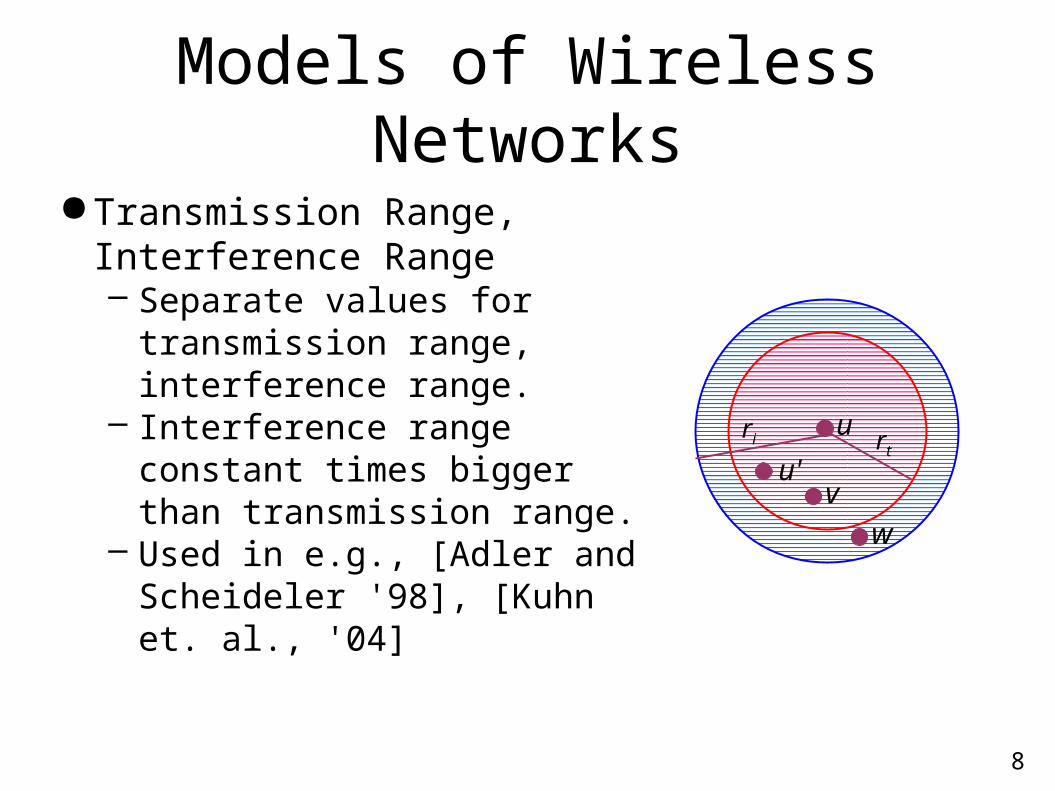
●Transmission Range, Interference Range– Separate values for transmission

range, interference range.– Interference range constant times

bigger than transmission range.– Used in e.g., [Adler and

Scheideler '98], [Kuhn et. al., '04]

Models of Wireless Networks

urt

vw

u'

ri

8

●Transmission Range, Interference Range– Separate values for transmission

range, interference range.– Interference range constant times

bigger than transmission range.– Used in e.g., [Adler and

Scheideler '98], [Kuhn et. al., '04]

●What is the problem?– Extension of unit disk model to

handle interference

Models of Wireless Networks

urt

vw

u'

ri

9

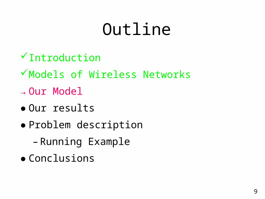
Outline

Introduction

Models of Wireless Networks

→Our Model

● Our results

● Problem description

– Running Example

● Conclusions

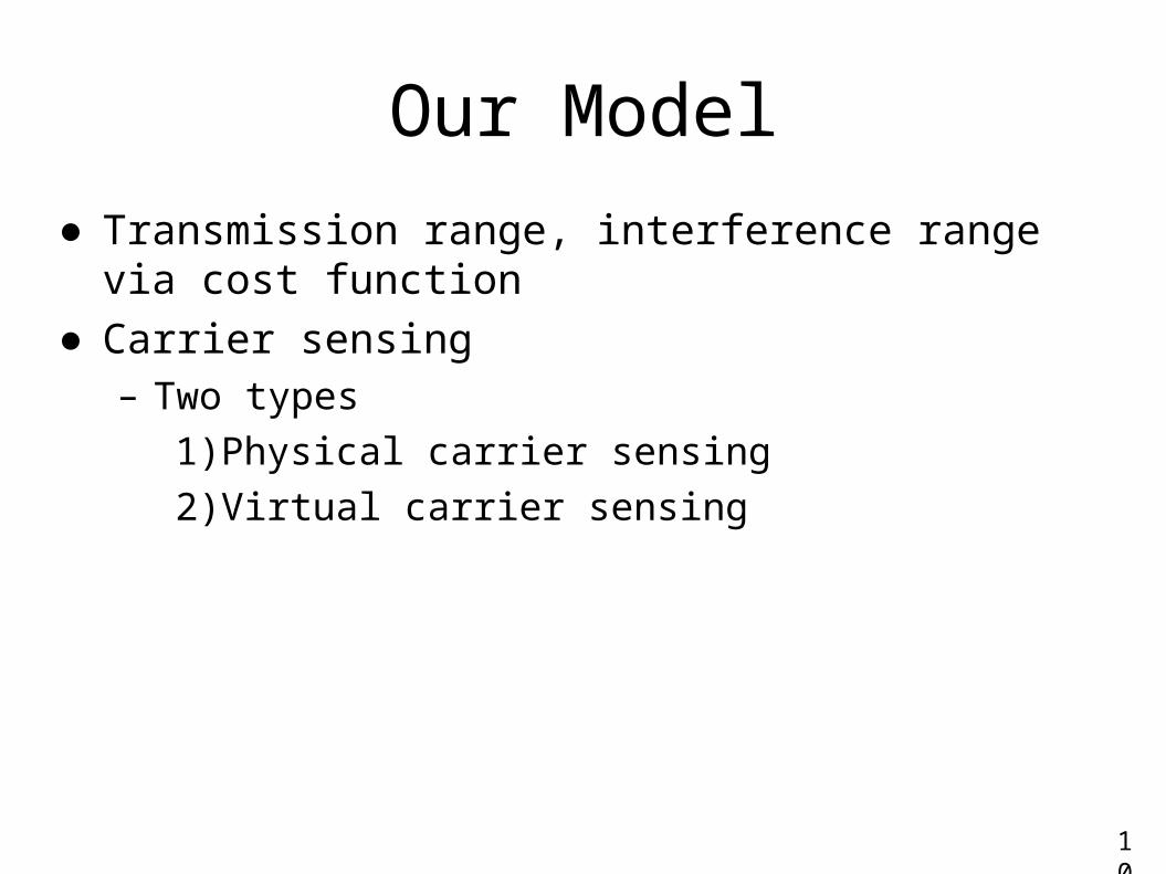
Our Model

● Transmission range, interference range via cost function

● Carrier sensing– Two types

1)Physical carrier sensing

2)Virtual carrier sensing

10

Cost Function

● Gr = (V, Er), set of nodes V, Euclidean distance d(•,•)● c is a cost function on nodes

– symmetric: c(u,v) = c(v,u)

− [0,1), depends on the environment

– c(u,v) [(1-)•d(u,v), (1+)•d(u,v)]

● Edge (u,v) Er if and only if c(u,v) ≤ r

w

u

va

b

11

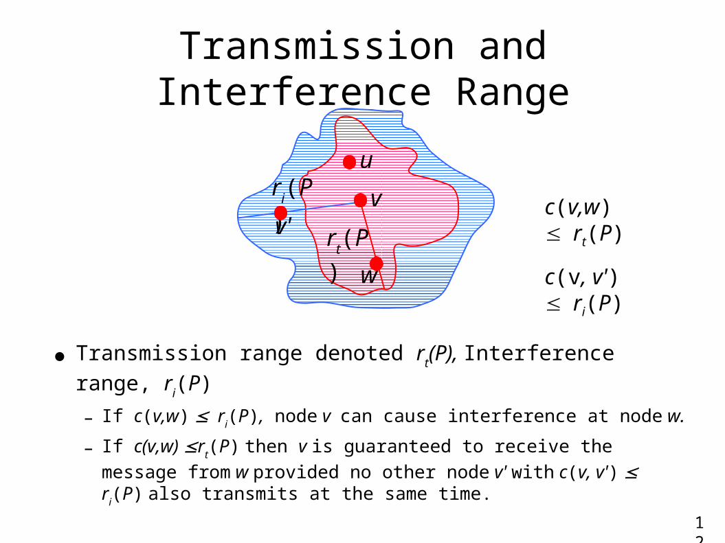
Transmission and Interference Range

● Transmission range denoted rt(P), Interference range, r

i(P)

– If c(v,w) ≤ ri(P), node v can cause interference at node w.

– If c(v,w) ≤rt(P) then v is guaranteed to receive the message from

w provided no other node v' with c(v, v') ≤ ri(P) also transmits at

the same time.

12

w

rt(P)v'

ri(P)

u

v c(v,w) rt(P)

c(v, v') ri(P)

Physical Carrier Sensing

● Provided by Clear Channel Assessment (CCA) circuit:– Monitor the medium as a function of Received Signal

Strength Indicator (RSSI)

– Energy Detection (ED) bit set to 1 if RSSI exceeds a certain threshold

– Has a register to set the threshold in dB

13

Physical Carrier Sensing

● Carrier sense transmission (CST) range, denoted rst(T, P)

● Carrier sense interference (CSI) range, denoted rsi(T, P)

● Both the ranges grow monotonically in both T and P.

w

vr

st(T,P)v'

v''

14

rsi(T,P) c(w,v) rst(T, P)

c(w, v') rsi(T, P)

c(w, v'') rsi(T, P)

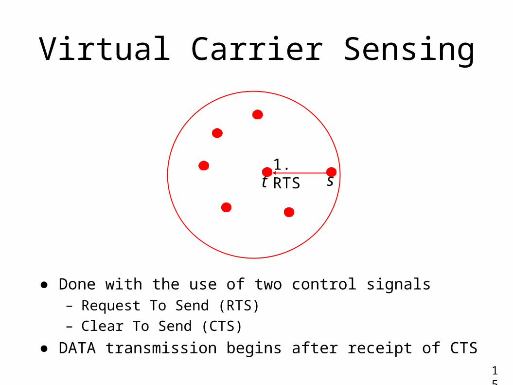
Virtual Carrier Sensing

1. RTSst

15

● Done with the use of two control signals – Request To Send (RTS)

– Clear To Send (CTS)

● DATA transmission begins after receipt of CTS

Virtual Carrier Sensing

● Done with the use of two control signals – Request To Send (RTS)

– Clear To Send (CTS)

● DATA transmission begins after receipt of CTS15

2. CTSst

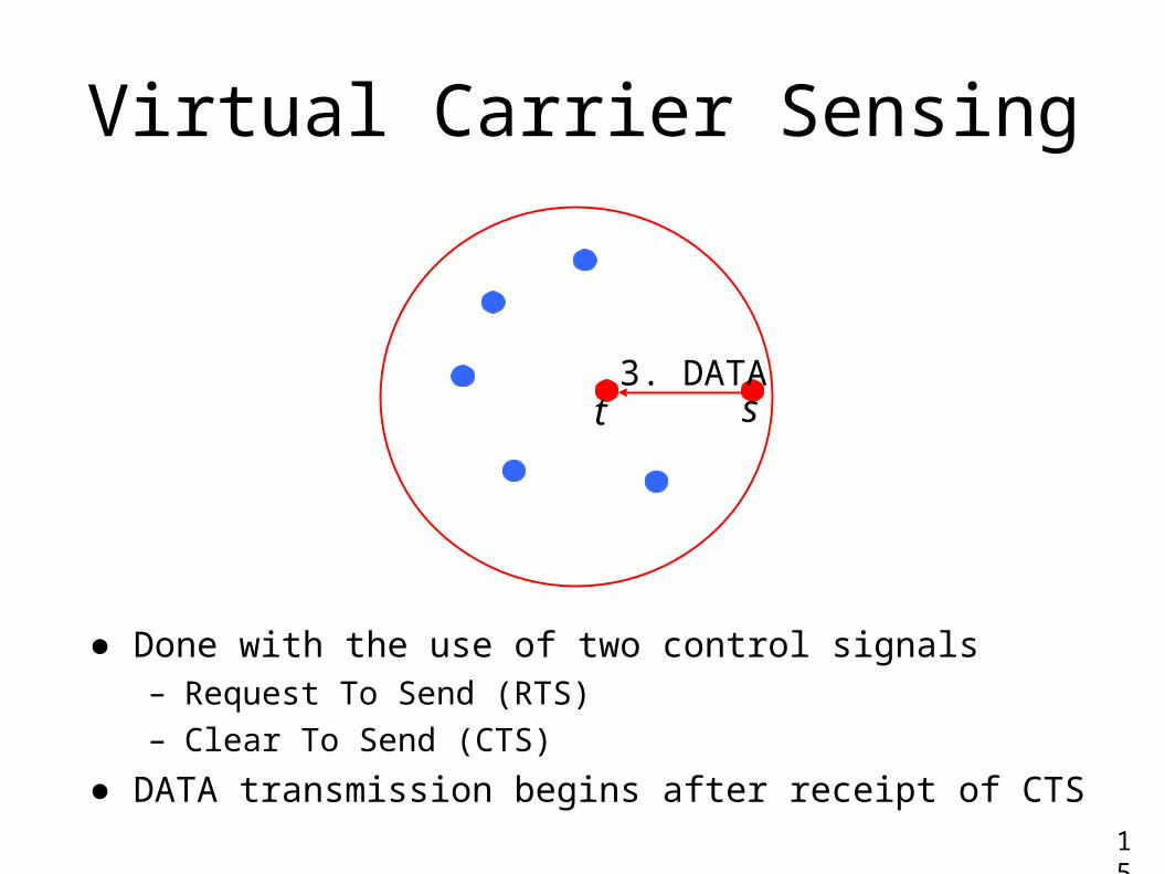
Virtual Carrier Sensing

15

3. DATAst

● Done with the use of two control signals – Request To Send (RTS)

– Clear To Send (CTS)

● DATA transmission begins after receipt of CTS

16

Outline

Introduction

Models of Wireless Networks

Our Model

→Our Results

● Problem description

– Running Example

● Conclusions

Our Results

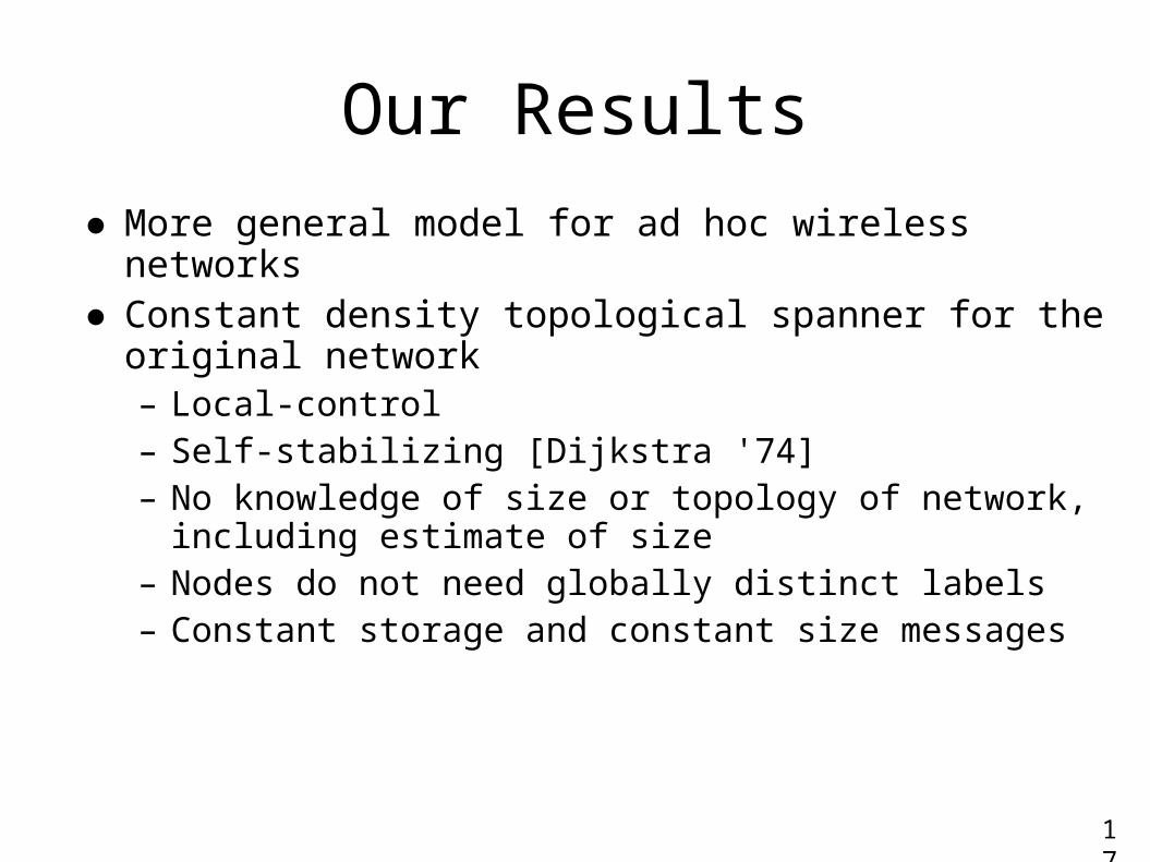
● More general model for ad hoc wireless networks● Constant density topological spanner for the original

network– Local-control– Self-stabilizing [Dijkstra '74]– No knowledge of size or topology of network, including

estimate of size– Nodes do not need globally distinct labels– Constant storage and constant size messages

17

18

Outline

Introduction

Models of Wireless Networks

Our Model

Our Results

→Problem Description

– Running Example

● Conclusions

Topological Spanners

● Definition: Given a graph G = (V,E), find a sub-graph H = (V, E') such that d

H(u,v) ≤ t•dG(u,v)

– H is also called a t-spanner.

● Previous Work– [Alzoubi et. al., '03] 5-spanner

– [Dubhashi et. al., '03] log n – spanner

19

Our Approach

20

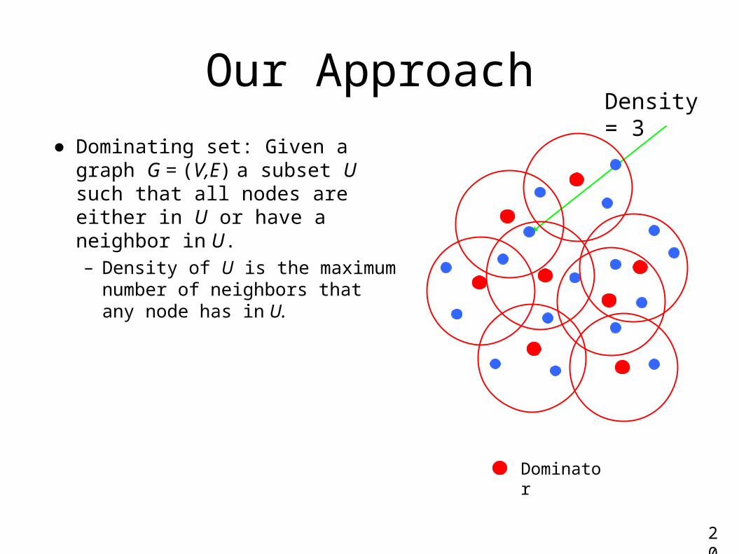
● Dominating set: Given a graph G = (V,E) a subset U such that all nodes are either in U or have a neighbor in U.– Density of U is the maximum

number of neighbors that any node has in U.

Dominator

Density = 3

● Seek a connected dominating set of constant density.

20

Our Approach

● Dominating set: Given a graph G = (V,E) a subset U such that all nodes are either in U or have a neighbor in U.– Density of U is the maximum

number of neighbors that any node has in U.

Dominator

Density = 3

Our Approach

● Each round has time slots reserved for each phase of the protocol

21

Time

One round

Phase I Phase II Phase III Phase I Phase II Phase III

● Three phase protocol1. Phase I: Dominating set2. Phase II: Distributed Coloring3. Phase III: Gateway Discovery

22

Outline

Introduction

Models of Wireless Networks

Our Model

Our Results

Problem Description

→Running Example

● Conclusions

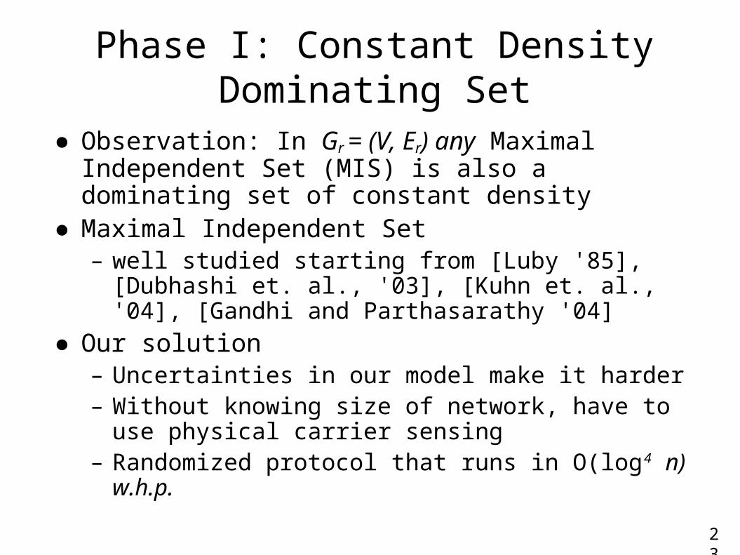
Phase I: Constant Density Dominating Set

● Observation: In Gr = (V, Er) any Maximal Independent Set (MIS) is also a dominating set of constant density

● Maximal Independent Set– well studied starting from [Luby '85], [Dubhashi et.

al., '03], [Kuhn et. al., '04], [Gandhi and Parthasarathy '04]

● Our solution– Uncertainties in our model make it harder– Without knowing size of network, have to use

physical carrier sensing– Randomized protocol that runs in O(log4 n) w.h.p.

23

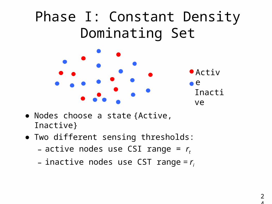
● Nodes choose a state {Active, Inactive}

● Two different sensing thresholds:

– active nodes use CSI range = rt

– inactive nodes use CST range = ri

24

InactiveActive

Phase I: Constant Density Dominating Set

● If an active node sends a LEADER signal, the nodes that receive/sense the leader signal stay inactive

Changed from Active Inactive

●Nodes choose a state {Active, Inactive}● Two different sensing thresholds:

– active nodes use CSI range = rt

– inactive nodes use CST range = ri

24

Inactive

Active and sent LEADER

Phase I: Constant Density Dominating Set

Phase I: Constant Density Dominating Set

DominatorsInactive nodes

● Nodes choose a state {Active, Inactive}● Two different sensing thresholds:

– active nodes use CSI range = rt

– inactive nodes use CST range = ri

● If an active node sends a LEADER signal, the nodes that receive/sense the leader signal stay inactive

● If no active node available, inactive nodes become active again

24

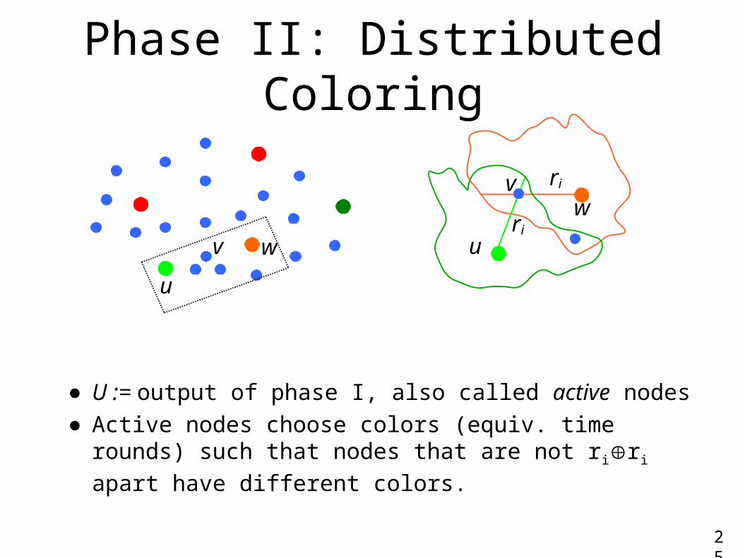
Phase II: Distributed Coloring

● U := output of phase I, also called active nodes● Active nodes choose colors (equiv. time rounds)

such that nodes that are not riri apart have

different colors.25

ri

ri

u

vw

u

v w

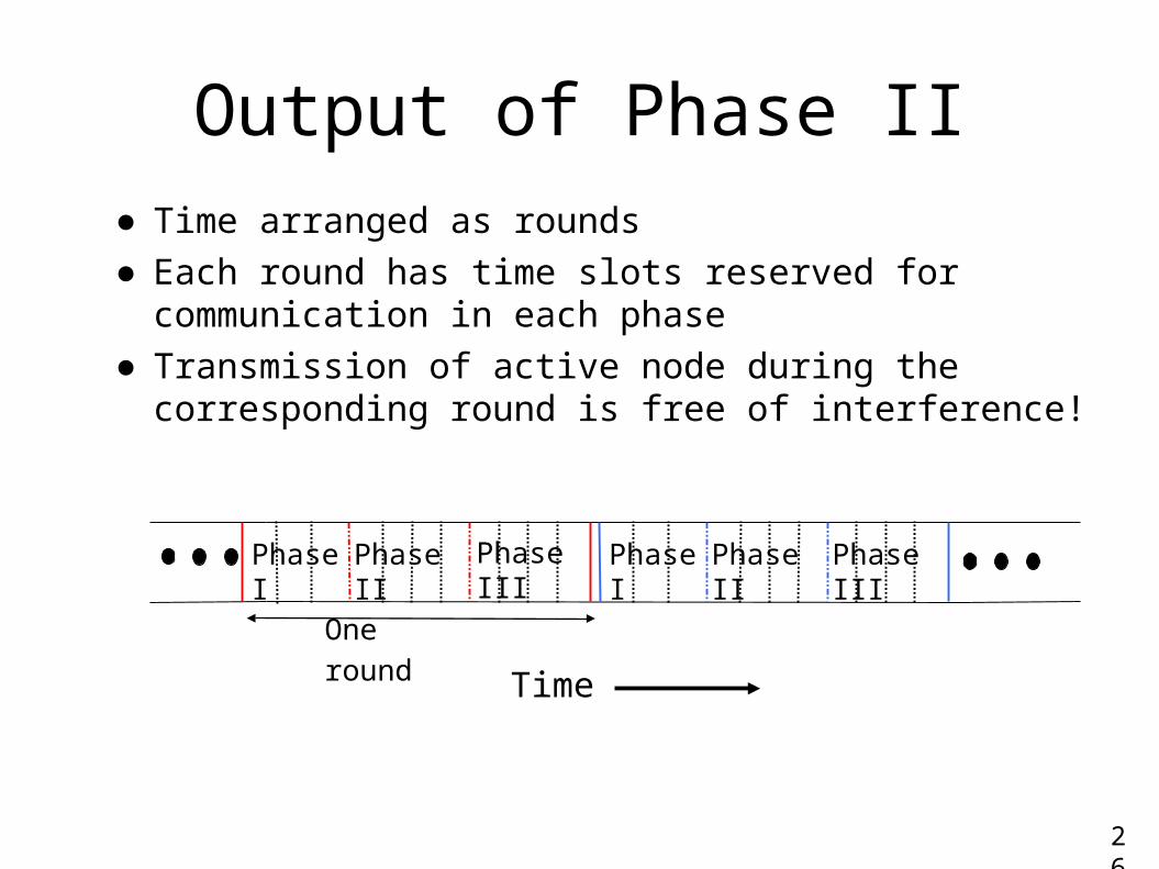
Output of Phase II

● Time arranged as rounds● Each round has time slots reserved for

communication in each phase● Transmission of active node during the

corresponding round is free of interference!

26

One round

Phase I Phase II Phase III Phase I Phase II Phase III

Time

Phase III: Gateway Discovery● Dominating set U may not be a connected

dominating set– Extend U by gateway nodes.

● Observation: Each node in U needs O(1) gateways.● Uses coloring achieved in Phase II to minimize

interference problems● Approach similar to that used in [Wang and Li, '03]

27

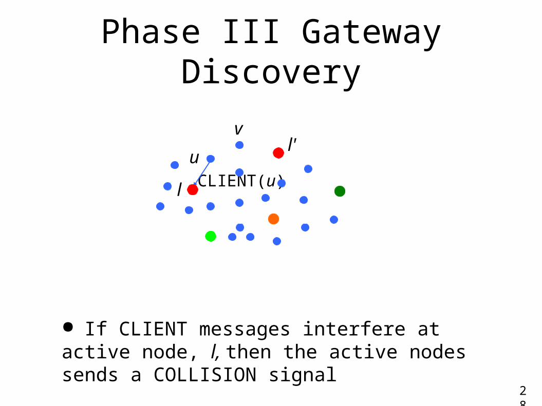
Phase III Gateway Discovery

u

l

l'

CLIENT(u)

v

● If CLIENT messages interfere at active node, l, then the active nodes sends a COLLISION signal

28

Phase III Gateway Discovery

ACK

● Eventually only one inactive node sends a CLIENT message to an active node

28

u

l

l'v

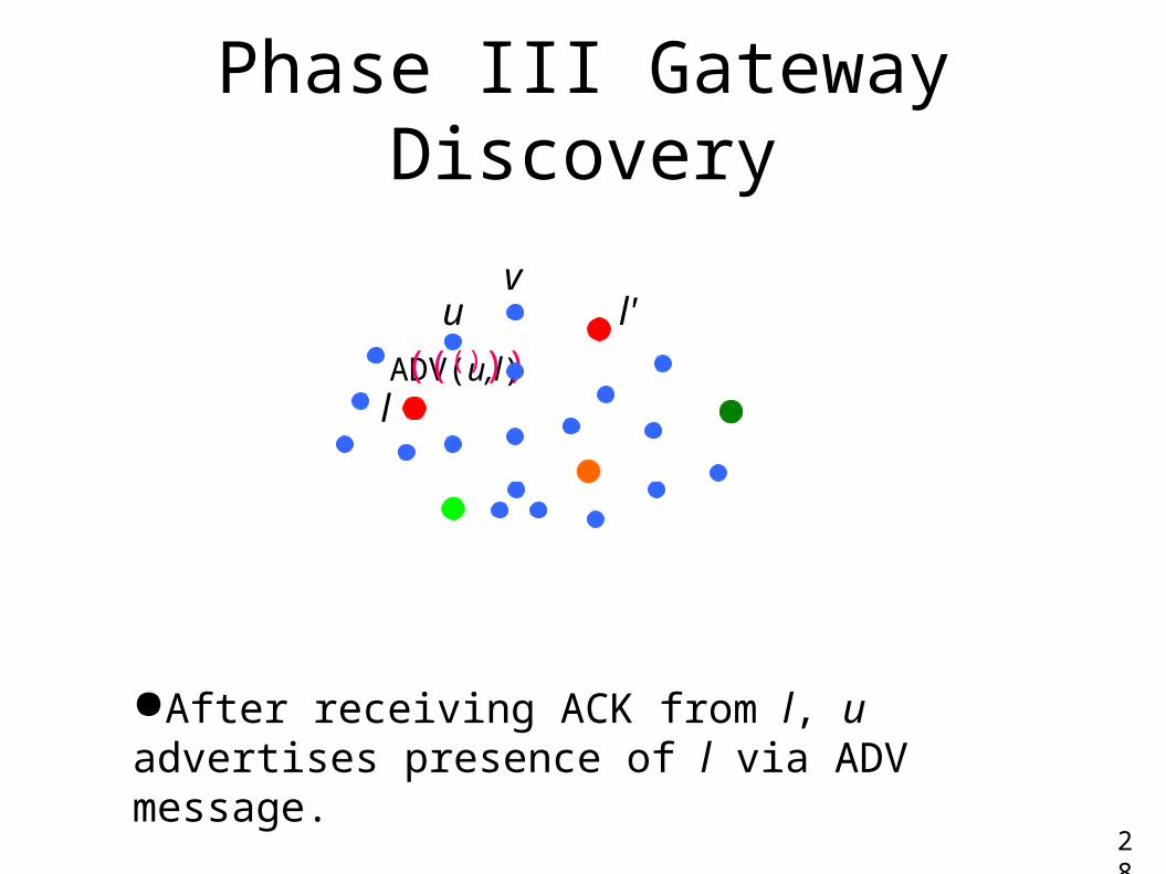
Phase III Gateway Discovery

28

●After receiving ACK from l, u advertises presence of l via ADV message.

ADV(u,l)((( )))

u

l

l'v

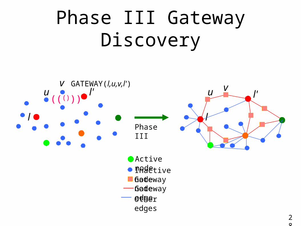
Phase III Gateway Discovery

Phase III

28

GATEWAY(l,u,v,l')

((( )))u

l

l'v

u

l

l'v

Active node

Inactive nodeGateway nodeGateway edgeOther edges

3-Spanner

● Our construction achieves a 3-spanner of constant density for the original network.

●Total runtime = O(log4 n + (D log D) log n) whp.– D is the density of the original network

29

u

l

l'v

st

Active node

Inactive nodeGateway nodeGateway edgeOther edges

30

Outline

Introduction

Models of Wireless Networks

Our Model

Our Results

Problem Description

Running Example

→Conclusions

Conclusions and Future Work

● More realistic model for wireless networks● Still possible to design efficient algorithms

– Constant density 3-spanner

– Algorithms are simple and use constant sized messages, constant storage at nodes

● Further applications– Higher communication primitives e.g., broadcasting,

gathering

– Handling mobility

31