Consistent modeling and e�cient pricing of

VIX options

A. Barletta

Department of Economics and Business Economics

Aarhus University

London, 14 March 2016

The research leading to these results has received funding from the European Union SeventhFramework Programme (FP7/2007-2013) under grant agreement n◦289032.

.

2 of 16 • Introduction 〉

Introduction

The Volatility Index (VIX) is a measure of market

volatility solely based on OTM option prices on the S&P

500.

It is determined as the square root of the value of a

portfolio that replicates the "fair" price of a 30-days (=τ)

variance swap.

The continuous time version of the VIX is the square root

of the log-price conditional annualized quadratic variation

VIX2t =

1

τEt

[[X ]t+τt

]:=

1

τlim

N→+∞Et

[N∑n=0

(log(St+n τ

N/St+(n−1) τ

N))2]

.

3 of 16 • Introduction 〉 Modeling VIX under SV

Modeling VIX under stochastic volatility

In our setting today's price of a VIX call option with strike K

and maturity T is always

C (K ,T ) = e−rTE[(VIXT −K )+

],

therefore we model the risk-neutral dynamics of the VIX.

The VIX has no explicit dependence on the stock price,

but they can be linked through the instantaneous variance

v .

A starting point is the Heston model

d log(St ) =(r −

vt

2

)dt +

√vtdZt

dvt = κ(θ− vt )dt + ε√vtdWt ,

d 〈Z ,W 〉t = ρdt .

4 of 16 • Introduction 〉 Modeling VIX under SV

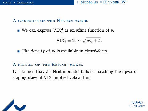
Advantages of the Heston model

We can express VIX2t as an a�ne function of vt

VIXt = 100 ·√avt + b.

The density of vt is available in closed-form.

A pitfall of the Heston model

It is known that the Heston model fails in matching the upward

sloping skew of VIX implied volatilities.

5 of 16 • Introduction 〉 Modeling VIX under SV

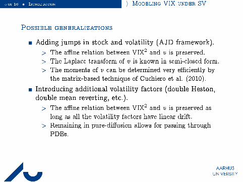
Possible generalizations

Adding jumps in stock and volatility (AJD framework).

> The a�ne relation between VIX2 and v is preserved.

> The Laplace transform of v is known in semi-closed form.

> The moments of v can be determined very e�ciently by

the matrix-based technique of Cuchiero et al. (2010).

Introducing additional volatility factors (double Heston,double mean reverting, etc.).

> The a�ne relation between VIX2 and v is preserved as

long as all the volatility factors have linear drift.

> Remaining in pure-di�usion allows for passing through

PDEs.

6 of 16 • SP1 - Affine jump-diffusion 〉

Subproject 1 - Pricing VIX under AJD

The AJD framework

Under the a�ne jump-di�usion (AJD) framework we have

d log(St ) =

(r − λµ−

1

2vt

)dt +

√vtdZt + dJXt ,

dvt = κ(θ− vt )dt + ε√vtdWt + dJ vt ,

d 〈Z ,W 〉t = ρdt ,

where J = (JX ,J v ) is a pure jump process taking values in

R× R+ and µ is the compensator of JX .

7 of 16 • SP1 - Affine jump-diffusion 〉 Orthogonal polynomial expansions

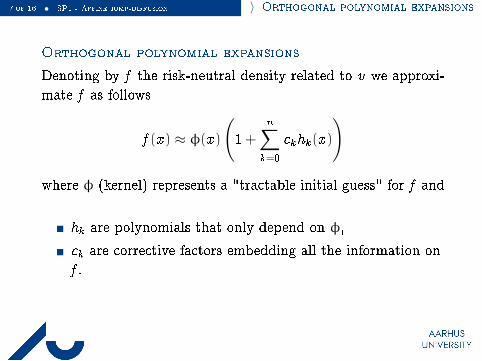
Orthogonal polynomial expansions

Denoting by f the risk-neutral density related to v we approxi-

mate f as follows

f (x ) ≈ φ(x )

(1+

n∑k=0

ckhk (x )

)

where φ (kernel) represents a "tractable initial guess" for f and

hk are polynomials that only depend on φ,

ck are corrective factors embedding all the information on

f .

8 of 16 • SP1 - Affine jump-diffusion 〉 Orthogonal polynomial expansions

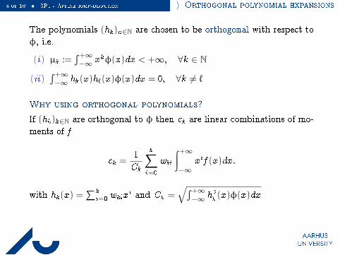
The polynomials (hk )n∈N are chosen to be orthogonal with respect to

φ, i.e.

(i) µk :=∫+∞−∞ x kφ(x )dx < +∞, ∀k ∈ N

(ii)∫+∞−∞ hk (x )h`(x )φ(x )dx = 0, ∀k 6= `

Why using orthogonal polynomials?

If (hk )k∈N are orthogonal to φ then ck are linear combinations of mo-

ments of f

ck =1

Ck

k∑i=0

wki

∫+∞−∞ x i f (x )dx .

with hk (x ) =∑

k

i=0wkix

i and Ck =√∫+∞

−∞ h2

k(x )φ(x )dx

9 of 16 • SP1 - Affine jump-diffusion 〉 Orthogonal polynomial expansions

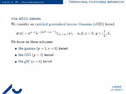
The eGIG kernel

We consider an enriched generalized inverse Gaussian (eGIG) kernel

φ(x ) = xα−1e−(βx p+γx−1)1[0,+∞)(x ), α, β, γ > 0, p ∈ (1

2, 1].

We focus on three subcases:

the gamma (p = 1, γ = 0) kernel

the GIG (p = 1) kernel

the gW (γ = 0) kernel

0.87 1 1.31 1.53 1.75 1.97 2.190.3

0.4

0.5

0.6

0.7

0.8

0.9T = 2 months

0.87 1 1.31 1.53 1.75 1.96 2.18

0.3

0.4

0.5

0.6

T = 4 months

0.87 1 1.31 1.53 1.74 1.96 2.18

0.25

0.3

0.35

0.4

0.45

0.5

T = 6 months

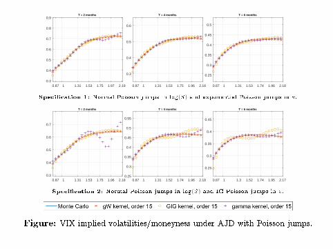
Speci�cation 1: Normal Poisson jumps in log(S) and exponential Poisson jumps in v .

0.87 1 1.31 1.53 1.75 1.96 2.180.3

0.4

0.5

0.6

0.7

T = 2 months

0.87 1 1.31 1.52 1.74 1.96 2.180.25

0.3

0.35

0.4

0.45

0.5

0.55

T = 4 months

0.87 1 1.3 1.52 1.74 1.95 2.17

0.25

0.3

0.35

0.4

0.45

T = 6 months

Speci�cation 2: Normal Poisson jumps in log(S) and IG Poisson jumps in v .

Figure: VIX implied volatilities/moneyness under AJD with Poisson jumps.

Efficiency

Under Speci�cation 2 we compare

Our technique (orders ranging from 10 to 20).

Laplace integration optimized formula of Lian and Zhu (2013).

Monte Carlo with Euler scheme on a time grid of 103 points/month.

10 11 12 13 14 15 16 17 18 19 20

Expansion order

10-1

100

101

102

103

Com

puta

tion

time

(sec

onds

)

Gamma kernel GW kernel GIG kernel Lian-Zhu MC (105 paths) MC (106 paths)

12 of 16 • SP2 - Multi-factor models 〉

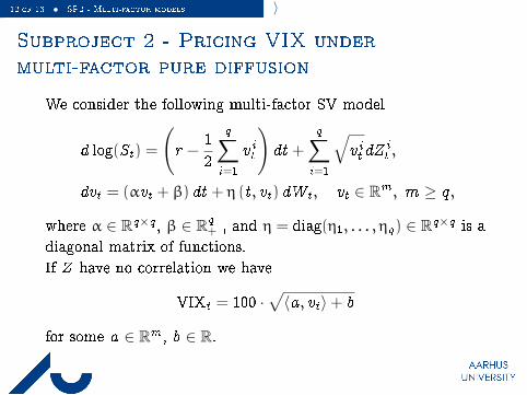
Subproject 2 - Pricing VIX under

multi-factor pure diffusion

We consider the following multi-factor SV model

d log(St ) =

(r −

1

2

q∑i=1

v it

)dt +

q∑i=1

√v it dZ

it ,

dvt = (αvt + β) dt + η (t , vt ) dWt , vt ∈ Rm , m ≥ q ,

where α ∈ Rq×q , β ∈ Rq+ , and η = diag(η1, . . . , ηq) ∈ Rq×q is a

diagonal matrix of functions.

If Z have no correlation we have

VIXt = 100 ·√〈a , vt 〉+ b

for some a ∈ Rm , b ∈ R.

13 of 16 • SP2 - Multi-factor models 〉

Some history:

Hagan and Woodward (1999) found asymptotics for the

implied volatilities under a CEV model based on a

PDE-technique.

Lorig et al. (2015) have recently extended this technique

to a broader pure-di�usion setting.

Based on this, Pagliarani and Pascucci (2016) have

extended these results to include the implied volatility

sensitivities.

We extend these results to a context where the underlying

(the VIX futures) dynamics are not explicit.

All these results apply to short-time and near ATM

options.

14 of 16 • Examples 〉

Examples

Introducing an elasticity coefficient in the

vol-of-vol

d log(St ) = −1

2vtdt +

√vtdW

Xt

dvt = k(vt − θ

h)dt + εhv δt dW

Yt

We have

limK→VIX0T→0

∂

∂Kσimp(T ,K ) =

εvδ− 1

20

(2δVIX2

0 − 2av0)

4VIX20

√v0

.

The slope is controlled by

2δVIX20 − 2av0 = 2(δ− 1)av0 + 2δb

15 of 16 • Examples 〉

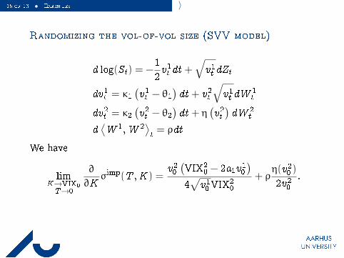
Randomizing the vol-of-vol size (SVV model)

d log(St ) = −1

2v1t dt +

√v1t dZt

dv1t = κ1(v1t − θ1

)dt + v2t

√v1t dW

1t

dv2t = κ2(v2t − θ2

)dt + η

(v2t)dW 2

t

d⟨W 1,W 2

⟩t= ρdt

We have

limK→VIX0T→0

∂

∂Kσimp(T ,K ) =

v20(VIX2

0 − 2a1v10

)4√v10VIX

20

+ ρη(v20 )

2v20.

16 of 16 • 〉

Thank you for your attention.