ORNL/TM-2012/7

Consistent Adjoint Driven Importance Sampling using Space, Energy, and Angle

August 2012 Prepared by Douglas E. Peplow Scott W. Mosher Thomas M. Evans

DOCUMENT AVAILABILITY

Reports produced after January 1, 1996, are generally available free via the U.S. Department of Energy (DOE) Information Bridge:

Web site: http://www.osti.gov/bridge Reports produced before January 1, 1996, may be purchased by members of the public from the following source:

National Technical Information Service 5285 Port Royal Road Springfield, VA 22161 Telephone: 703-605-6000 (1-800-553-6847) TDD: 703-487-4639 Fax: 703-605-6900 E-mail: info@ntis.fedworld.gov Web site: http://www.ntis.gov/support/ordernowabout.htm

Reports are available to DOE employees, DOE contractors, Energy Technology Data Exchange (ETDE) representatives, and International Nuclear Information System (INIS) representatives from the following source:

Office of Scientific and Technical Information P.O. Box 62 Oak Ridge, TN 37831 Telephone: 865-576-8401 Fax: 865-576-5728 E-mail: reports@adonis.osti.gov Web site: http://www.osti.gov/contact.html

This report was prepared as an account of work sponsored by an agency of the United States Government. Neither the United States government nor any agency thereof, nor any of their employees, makes any warranty, express or implied, or assumes any legal liability or responsibility for the accuracy, completeness, or usefulness of any information, apparatus, product, or process disclosed, or represents that its use would not infringe privately owned rights. Reference herein to any specific commercial product, process, or service by trade name, trademark, manufacturer, or otherwise, does not necessarily constitute or imply its endorsement, recommendation, or favoring by the United States Government or any agency thereof. The views and opinions of authors expressed herein do not necessarily state or reflect those of the United States Government or any agency thereof.

ORNL/TM-2012/7

Reactor and Nuclear Systems Division

CONSISTENT ADJOINT DRIVEN IMPORTANCE SAMPLING USING SPACE, ENERGY AND ANGLE

Douglas E. Peplow Scott W. Mosher

Thomas M. Evans

Date Published: February 2012

Prepared by OAK RIDGE NATIONAL LABORATORY

Oak Ridge, Tennessee 37831-6283 managed by

UT-BATTELLE, LLC for the

U.S. DEPARTMENT OF ENERGY under contract DE-AC05-00OR22725

iii

CONTENTS

Page LIST OF FIGURES ................................................................................................................................ v

LIST OF TABLES ............................................................................................................................... vii

ACRONYMS AND ABBREVIATIONS .............................................................................................. ix

ACKNOWLEDGMENTS ..................................................................................................................... xi

ABSTRACT ........................................................................................................................................ xiii

1. INTRODUCTION .......................................................................................................................... 1

2. BACKGROUND ............................................................................................................................ 2 2.1 CADIS REVIEW ................................................................................................................... 2 2.2 SPACE/ENERGY CADIS FOR MULTIPLE SOURCES ..................................................... 3 2.3 WHEN SPACE/ENERGY CADIS IS NOT APPROPRIATE .............................................. 3 2.4 APPROXIMATE TREATMENT OF ANGULAR DEPENDENCE IN

IMPORTANCE MAPS .......................................................................................................... 5

3. DIRECTIONAL CADIS ................................................................................................................ 7 3.1 DIRECTIONALLY DEPENDENT WEIGHT WINDOWS WITHOUT

DIRECTIONAL SOURCE BIASING ................................................................................... 7 3.1.1 Theory ......................................................................................................................... 7 3.1.2 Implementation ........................................................................................................... 9 3.1.3 Extension to Multiple Sources .................................................................................. 10

3.2 DIRECTIONALLY DEPENDENT WEIGHT WINDOWS WITH DIRECTIONAL SOURCE BIASING ................................................................................. 11 3.2.1 Theory ....................................................................................................................... 11 3.2.2 Implementation ......................................................................................................... 12 3.2.3 Extension to Multiple Sources .................................................................................. 13

3.3 SCALE/MAVRIC SPECIFICS ............................................................................................ 14

4. APPLICATION EXAMPLES ...................................................................................................... 15 4.1 SPHERICAL BOAT TEST PROBLEM .............................................................................. 15 4.2 SIMPLE DUCT STREAMING PROBLEM ....................................................................... 16 4.3 UEKI SHIELDING PROBLEM .......................................................................................... 17 4.4 NEUTRON WELL-LOGGING PROBLEM ....................................................................... 18 4.5 GAMMA-RAY WELL-LOGGING PROBLEM ................................................................. 18 4.6 ACTIVE INTERROGATION BARREL PROBLEM ......................................................... 18 4.7 CARGO CONTAINER B PROBLEM ................................................................................ 19

5. CONCLUSIONS .......................................................................................................................... 21

6. REFERENCES ............................................................................................................................. 23

v

FIGURES

Figure Page

1 Elevation view of the spherical boat model showing the source (left) and the fissionable material at the center of the boat. ........................................................................ 4

2 Target weight window values for 14.1 MeV neutrons along the beam into the spherical boat computed by space/energy CADIS. Target weight at the source location is 1. .......................................................................................................................... 5

3 Target weight window values for 14.1 MeV neutrons as a function of distance from the center for the spherical boat. The source is located at −195 cm and the hull is at −90 cm. ................................................................................................................................ 15

4 Target weight window values for 14.1 MeV neutrons as a function of distance from the center for the spherical boat. The source is located at −1025 cm and the hull is at −90 cm. ................................................................................................................................ 16

5 Duct streaming problem target weight values for the 0.9–1.4 MeV group. The source is at the lower-left duct entrance, and the dose rate is calculated at the exit duct on the upper right. .......................................................................................................................... 17

6 Interrogation geometry for a barrel (57 cm diam, 85 cm high), with a source (S) on the left side and a detector (D) on the right. The 25 kg sphere of HEU sits at the bottom of the barrel. ............................................................................................................................. 19

7 A 12 m (40 ft) sealand cargo container 1 m above a concrete roadbed with a detector (D) in the foreground and a source on opposite side. .......................................................... 20

vii

TABLES

Table Page

1 Results for a simple duct streaming problem .......................................................................... 17 2 Effectiveness summary—Ratio of the Monte Carlo FOM (angular CADIS to standard

CADIS) for eight simple problems.......................................................................................... 21

ix

ACRONYMS AND ABBREVIATIONS

ADVANTG Automated Variance Reduction Generator AVATAR Automatic Variance and Time of Analysis Reduction FW-CADIS Forward-Weighted Consistent Adjoint Driven Importance Sampling CADIS Consistent Adjoint Driven Importance Sampling FOM figure-of-merit HEU highly-enriched uranium MAVRIC Monaco with Automated Variance Reduction using Importance Calculations MC Monte Carlo MCNP Monte Carlo N-Particle pdf probability distribution function ORNL Oak Ridge National Laboratory

xi

ACKNOWLEDGMENTS

This work was sponsored by the Defense Threat Reduction Agency; the National Nuclear Security Administration, Office of Defense Nuclear Nonproliferation, Office of Nonproliferation R&D (NA-22); and the U.S. Nuclear Regulatory Commission, Office of Nuclear Reactor Regulation. ORNL is managed and operated by UT-Battelle, LLC, for the US Department of Energy under Contract No. DE-AC05-00OR22725.

xiii

ABSTRACT

For challenging radiation transport problems, hybrid methods combine the accuracy of Monte Carlo methods with global information present in deterministic methods. One of the most successful hybrid methods is CADIS – Consistent Adjoint Driven Importance Sampling. This method uses a deterministic adjoint solution to construct a biased source distribution and consistent weight windows to optimize a specific tally in a Monte Carlo calculation. The method has been implemented into transport codes using just the spatial and energy information from the deterministic adjoint solution and has been used in many applications to compute tallies with much higher figures-of-merit than analog calculations. CADIS also outperforms user-supplied importance values, which usually take long periods of user time to develop. This work extends CADIS to develop weight windows that are a function of the position, energy, and direction of the Monte Carlo particle. Two types of consistent source biasing are presented: one method that biases the source in space and energy while preserving the original directional distribution, and one method that biases the source in space, energy, and direction. Seven simple example problems are presented which compare the use of the standard space/energy CADIS with the two new space/energy/angle treatments.

1

1. INTRODUCTION

Monte Carlo (MC) simulation is being increasingly used for more challenging problems that require variance reduction techniques to obtain results with acceptably low statistical uncertainties in reasonable computational times. One of the best methods of variance reduction is the weight windows technique, in which target weights are assigned throughout the problem as a function of the MC particle parameters. If the weight of a particle is too low, roulette is played with surviving particles having an increased weight. If the particle weight is too high, splitting is used to create several lower-weight particles. If all of the particles passing through a given area of phase space have similar weights, the statistical variances of the tallies will be lower. If more particles are simulated in the important phase space areas of the problem and fewer particles in the unimportant areas, then the efficiency of the MC simulation is increased, reducing variances for a fixed amount of computation time. The difficult part of this approach is the assignment of target weights, which should be inversely proportional to the particle’s importance to the tally/response of interest. The adjoint flux obtained from the solution of an adjoint problem, using the tally response function as the adjoint source, is the importance of a MC particle at any phase space location to that tally. Because of this correspondence, weight windows have been constructed from adjoint solutions for some time now. One method that uses this concept is Consistent Adjoint Driven Importance Sampling (CADIS), developed by Wagner and Haghighat,1 which also includes a biased source designed to work in conjunction with the weight windows. Very large increases in the MC figure-of-merit (FOM) can be achieved for deep penetration source-detector problems using their approach. This method and its extensions for computing global quantities, Forward-Weighted CADIS (FW-CADIS),2 have been very successful in many applications: spent fuel cask dose rates, dose rates over an entire pressurized-water reactor facility, active interrogation modeling, and doses from detonations of nuclear weapons in urban areas. These CADIS methods and applications have all used weight windows and source biasing based on only the spatial and energy dimensions of the adjoint calculation. For some applications, the particle importance at a given location in space and a given energy may also be highly dependent on the particle direction. For example, a particle streaming through a duct has a very different importance to a detector tally from a particle with the same position and energy but traveling perpendicular to that duct. The current implementation of CADIS would miss this difference, instead assigning both particles the same importance independent of the particle direction. This paper develops the methods and implementations for using some of the angular information present in the deterministic adjoint calculation for the formulation of space/energy/angle CADIS. Two methods are developed: one method that does not bias the directional component of the source distribution (suitable for beam problems) and one that does bias the source distribution directional component. The results of these methods, particularly the improvement of the MC FOM, are compared with the standard space/energy CADIS for seven simple example problems.

2

2. BACKGROUND 2.1 CADIS REVIEW

Wagner and Haghighat3 developed and fully described CADIS, so only a brief review will be given here. For the MC calculation of some response , using the response function , , Ω to determine total flux, dose, etc., over some detector region from a unit source, where = , , Ω , , Ω Ω , (1)

particles are sampled from the source distribution , , Ω , transported through the geometry, and tallied with the response function in the appropriate portion of phase space. Equivalently, the response can also be found from integrating the true source with the adjoint fluxes , , Ω , i.e. = , , Ω , , Ω Ω , (2)

where the adjoint calculation used the adjoint source of , , Ω = , , Ω . To minimize the variance in the MC calculation of , Wagner and Haghighat showed that the biased source distribution of , , Ω = 1 , , Ω , , Ω (3)

should be used. If the adjoint solution was known exactly, then this biased source would yield a zero-variance estimate of . A good estimate of the adjoint fluxes should significantly reduce the variance in calculating . Particles sampled from the biased distribution are born with a weight of ≡ ⁄ . A set of weight window target values can be constructed to match these birth weights by using , , Ω = , , Ω . (4)

CADIS is implemented by first estimating the adjoint flux , , Ω , integrating the adjoint flux and true source distribution to estimate , and then forming the biased source distribution and weight window target values for use in the MC calculation. Note that this formulation of the weight window target values using Eq. (4) makes the importance map “consistent” with the biased source—a source particle is born with an initial weight matching the target weight value of the location and energy where it is born. As a result, unnecessary rouletting and splitting just after starting a source particle are avoided, thus increasing the calculational efficiency. For a system using a deterministic method to compute the adjoint fluxes, this completely general space/energy/angle approach presents many difficulties in implementation, such as

• dealing with the large amount of memory required for a , , Ω importance map in memory; • interpolating the importance for directions in between quadrature angles; and • expressing the biased source in a form suitable for a general MC code, because the above

biased source is in general not separable. A space/energy version of CADIS has been implemented in both the ADVANTG4 (Automated Variance Reduction Generator) code system for MCNP5 and in the MAVRIC (Monaco with

3

Automated Variance Reduction using Importance Calculations) sequence6 of SCALE.7 Both of these implementations use the adjoint scalar fluxes produced by the Denovo SN code.8 The resulting importance map is a function only of space and energy, and the source is biased only in space and energy, preserving the original direction distribution of the true source. An aim of both ADVANTG and MAVRIC is to be as automatic as possible. The user creates the same input file as for an analog MC calculation and then provides extra information for the discrete ordinates adjoint calculation. This extra information consists of the mesh and the adjoint source spatial and energy distributions, which should correspond to the tally that the user wishes to optimize. Default parameters for the Denovo calculation, such as quadrature order, Legendre order, and upscatter capability can also be overridden by the user. ADVANTG and MAVRIC then use the information to construct a voxelized version of the geometry and adjoint source, relieving the user of the task of preparing multiple models for SN and MC codes. 2.2 SPACE/ENERGY CADIS FOR MULTIPLE SOURCES

For a typical MC calculation with multiple sources, each with a probability distribution function , and a strength (giving a total source strength of = ∑ ), the total source is sampled in two steps. First, the individual source i is sampled with probability = / ,and then the particle is sampled from the individual source distribution , . In developing the biased source distributions and weight windows, the response due to each source, , is used and the results are

= , , , (5)

= ∑ , (6)

, = 1 , , , (7)

, = ∑ 1, . (8)

Note that the biased distribution of which source to pick, , is based on the contribution of each individual source, , to the total response, ∑ . Sources are sampled in direct proportion to their contribution to the desired tally by first sampling which of the individual sources to use with and then sampling the ith biased source, , . 2.3 WHEN SPACE/ENERGY CADIS IS NOT APPROPRIATE

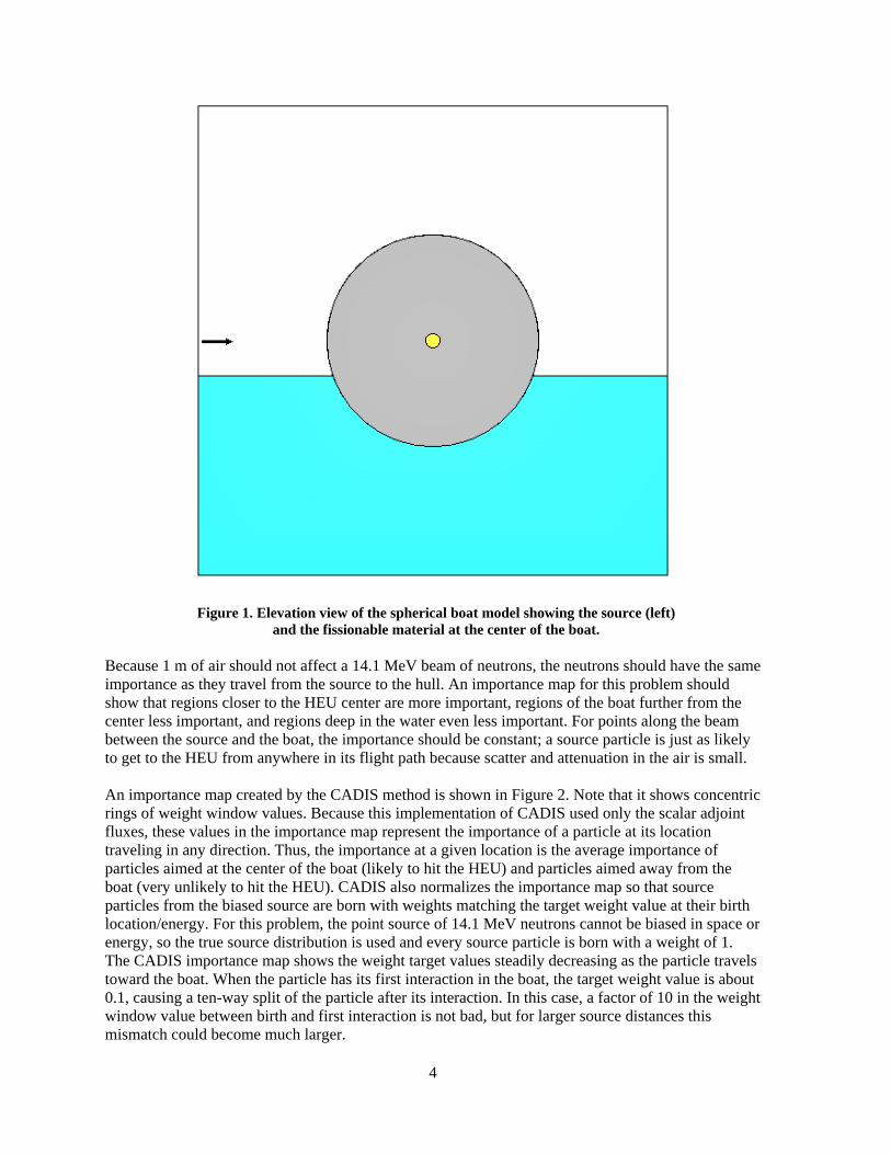
Consider the following idealized problem of a spherical boat floating in a large body of seawater, as shown in Figure 1. The boat consists of a homogenized mixture of typical boat materials, air, and water with a sphere of highly-enriched uranium (HEU) at its center. An active interrogation source is that consists of a beam 2° wide of 14.1 MeV neutrons. The source is 1 m from the boat’s hull and strikes the hull in line with its center. The goal is to determine the fission rate induced by the interrogation beam.

4

Figure 1. Elevation view of the spherical boat model showing the source (left) and the fissionable material at the center of the boat.

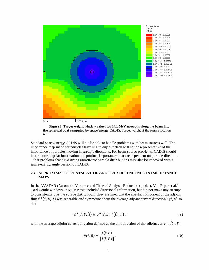
Because 1 m of air should not affect a 14.1 MeV beam of neutrons, the neutrons should have the same importance as they travel from the source to the hull. An importance map for this problem should show that regions closer to the HEU center are more important, regions of the boat further from the center less important, and regions deep in the water even less important. For points along the beam between the source and the boat, the importance should be constant; a source particle is just as likely to get to the HEU from anywhere in its flight path because scatter and attenuation in the air is small. An importance map created by the CADIS method is shown in Figure 2. Note that it shows concentric rings of weight window values. Because this implementation of CADIS used only the scalar adjoint fluxes, these values in the importance map represent the importance of a particle at its location traveling in any direction. Thus, the importance at a given location is the average importance of particles aimed at the center of the boat (likely to hit the HEU) and particles aimed away from the boat (very unlikely to hit the HEU). CADIS also normalizes the importance map so that source particles from the biased source are born with weights matching the target weight value at their birth location/energy. For this problem, the point source of 14.1 MeV neutrons cannot be biased in space or energy, so the true source distribution is used and every source particle is born with a weight of 1. The CADIS importance map shows the weight target values steadily decreasing as the particle travels toward the boat. When the particle has its first interaction in the boat, the target weight value is about 0.1, causing a ten-way split of the particle after its interaction. In this case, a factor of 10 in the weight window value between birth and first interaction is not bad, but for larger source distances this mismatch could become much larger.

5

Figure 2. Target weight window values for 14.1 MeV neutrons along the beam into the spherical boat computed by space/energy CADIS. Target weight at the source location is 1.

Standard space/energy CADIS will not be able to handle problems with beam sources well. The importance map made for particles traveling in any direction will not be representative of the importance of particles moving in specific directions. For beam source problems, CADIS should incorporate angular information and produce importances that are dependent on particle direction. Other problems that have strong anisotropic particle distributions may also be improved with a space/energy/angle version of CADIS. 2.4 APPROXIMATE TREATMENT OF ANGULAR DEPENDENCE IN IMPORTANCE

MAPS

In the AVATAR (Automatic Variance and Time of Analysis Reduction) project, Van Riper et al.9 used weight windows in MCNP that included directional information, but did not make any attempt to consistently bias the source distribution. They assumed that the angular component of the adjoint flux , , Ω was separable and symmetric about the average adjoint current direction , so that , , Ω ≅ , Ω ∙ , (9)

with the average adjoint current direction defined as the unit direction of the adjoint current, , , , = ,, . (10)

6

Note that the adjoint current direction points in the direction of increasing importance. The average cosine, , , of scatter is the ratio of the magnitude of the adjoint current to the scalar adjoint flux , = , , . (11)

Using information theory and the maximum entropy distribution, the function describing the shape of the azimuthally symmetric current at , was given as the probability distribution function = 2 sinh , (12)

with the single parameter , defined as

= 2.99821 − 2.2669248 1 − 0.769332 − 0.519928 + 0.2691594 ∈ 0, 0.800111 − ∈ 0.8001, 1 . (13)

The weight window target value for a particle at location , of energy , and traveling in direction Ω, is then , , Ω = , Ω ∙ , (14)

where the constant is chosen to match the source distribution as closely as possible. The authors noted that the approximation to the angular adjoint flux used above is exact in the limits of isotropic adjoint flux and in streaming cases. The authors did not report how they normalized the importance map to the source, if at all. Note that because is a probability distribution function in only, it may have been better to separate the polar and azimuthal components of the directional distribution and write

, , Ω ≅ , Ω (15)

= , 12 Ω ∙ , (16)

so that , Ω ∙ Ω = , . Evans and Hendricks10 compared the AVATAR approach (weight windows on a mesh developed by an SN code) with several flavors of weight window generation available within MCNP. Most of the non-AVATAR methods required lengthy iterations within MCNP. The only drawback the authors found against the AVATAR method was the preparation of the input for the SN code and the expertise required to use it. Modern implementations of CADIS in MAVRIC and the ADVANTG system for MCNP are much easier on the user. These codes create the SN code input, run the SN code, and create the importance map and biased sources automatically.

7

3. DIRECTIONAL CADIS

Completely general space/energy/angle CADIS is expected to be difficult to implement and may not be necessary for most applications. In many real problems involving directionally dependent source distributions, the directional dependence is azimuthally symmetric about some reference direction, . The angular distribution, Ω , can be expressed as the product of the uniform azimuthal distribution

and a polar distribution about reference direction giving Ω ∙ . The geometric size of these

sources tends to be small, allowing each source distribution to be expressed as the product of two separable distributions: , , Ω ≅ , Ω . A CADIS method is needed that (1) can account for the importance of a particle traveling in a certain direction, (2) can be cast as a simple modification of the space/energy CADIS method, and (3) is simpler than the full space/angle/energy approach. This can be accomplished by starting with the approximation that the angular component of the adjoint flux , , Ω is separable and symmetric about the average adjoint current direction , , so that , , Ω ≅ , 12 Ω ∙ . (17)

This is similar to the AVATAR approach but explicitly includes the azimuthal distribution so that the

standard definition , Ω ∙ Ω = , applies. From this, we can propose that

weight window targets be developed that are inversely proportional to the approximation of the adjoint angular flux , , Ω = 2, Ω ∙ , (18)

where is the constant of proportionality that will be adjusted to make the importance map consistent with the biased source(s). Two methods will be examined here, one without and one with biasing of the source directional dependence. For both of the new methods, the SN code Denovo was modified to report not only the adjoint scalar fluxes, , , but also the adjoint net currents in , , and directions: , , , , and , . The following methods have been developed so that the standard CADIS routines can be used to compute space/energy quantities of the response per unit source , the weight window target values , , and biased source , with just the adjoint scalar fluxes. These quantities are then modified by the directional information. 3.1 DIRECTIONALLY DEPENDENT WEIGHT WINDOWS WITHOUT DIRECTIONAL

SOURCE BIASING

3.1.1 Theory

We propose that the biased source , , Ω should be proportional to both the true source distribution and the space/energy component of the adjoint flux , , Ω = 1 , 12 Ω ∙ , , (19)

8

where the constant of proportionality, , is determined by forcing , , Ω to be a probability distribution function (pdf). Because the angular component of the adjoint flux is not included, the directional distribution of the biased source will be exactly the same as the true source. Note that this approach would be exact for cases where no directional biasing could be applied—mono-directional beam sources. The constant is found to be equal to

= , 12 Ω ∙ , Ω , (20)

= , , 12 Ω ∙ Ω .

(21)

Because the second integral is always 1, this is the same as the response per unit source from the traditional space/energy CADIS treatment. So, this biased source can be expressed using the space/energy biased source and the original directional distribution: , , Ω = , 12 Ω ∙ . (22)

The birth weight of a particle sampled from this distribution will be independent of direction and is ≡ , , Ω, , Ω = , . (23)

The proportionality constant, , in Eq. (18) for the target weight windows should be chosen to make the weight window targets match the birth weight of the source particles. This cannot be done in general because the birth weight is independent of direction, but it can be done for one point in phase space , , Ω of the source, so that

, , Ω = , , Ω , (24)

2 , Ω ∙ , = , ,

(25)

= 2 Ω ∙ , ,

(26)

where the average adjoint current direction , is evaluated at the source location/energy. Because the biased source and the weight window targets will match only at the specified direction of interest Ω at one specific position and energy, that point , , Ω should be chosen carefully to represent the entire source well and to minimize the rouletting or splitting of particles just after birth. In summary, for a separable source distribution, the CADIS method can be modified to use direction in the importance map but without source biasing to become

= , , , (27)

, , Ω =

1 , , 12 Ω ∙ = , 12 Ω ∙ , (28)

9

, , Ω = , Ω ∙ ,Ω ∙ = , Ω ∙ , Ω ∙ . (29)

The evaluation of the constant here is the same as that used for space/energy CADIS, but the weight window targets and biased source distribution are modifications of the space/energy CADIS

versions of those quantities. Also note that Ω ∙ , used here could be evaluated once and

made a part of the scaling of the space/energy weight window targets. 3.1.2 Implementation

Recall that this method uses the true angular source distribution for the biased source distribution. The user selects one point in phase space , , Ω that is representative of the entire source, where the biased source will match the target weight windows. The vector = , at that point is used to compute Ω ∙ , which is then multiplied by the target weight windows. The three adjoint net currents are passed along to the importance map for use in the MC transport. In the forward MC calculation, source particles are sampled from the biased source distribution , , with a direction about sampled using the original directional distribution Ω ∙ . Particle weight at birth is assigned to be ≡ ,, = , . (30)

Just after birth and during transport in the MC code, a weight check of a particle at , of energy , traveling in direction Ω is performed using the space/energy weight window target value , and the three partial adjoint currents using the logic below:

total current , = , + , + , average cosine , = , ,

if , > min, then the adjoint flux was not isotropic, so lambda

parameter = 2.99821 − 2.2669248 1 − 0.769332 − 0.519928 + 0.2691594 ∈ 0,0.800111 − ∈ 0.8001, 1

average adjoint

current vector , = ⟨ , , , , , ⟩ ,

cosine = Ω ∙

target value , , Ω = , ⁄

if , ≤ min, then the adjoint flux was close to isotropic, so

10

target value , , Ω = 2 , . Another approach for the weight window check would be to compute the values of , and , everywhere on the mesh when the target weight windows are constructed. Instead of storing the three partial adjoint currents (three double precision values), the quantities , and , could be stored (total of four values) but only in single precision, reducing the memory requirement and reducing the above computation to

if , > min, then the adjoint flux was not isotropic, so Cosine = Ω ∙

target value , , Ω = , ⁄

if , ≤ min, then the adjoint flux was close to isotropic, so target value , , Ω = 2 , .

A reasonable value for min, where the directional distribution of the adjoint flux could be considered isotropic, would be about 0.1, where min = 0.30186 and the resulting distribution of varies only between 0.36 and 0.66 for ∈ −1,1 . 3.1.3 Extension to Multiple Sources

The directional CADIS method without directional source biasing can easily be extended to multiple sources (each with a probability distribution function , , Ω and a strength , giving a total source strength of = ∑ ). The user is required to provide one point in phase space , , Ω for each source that is representative of that entire source, where the biased source will match the target weight windows. For each source, a vector = , is computed using that point. Each biased source , , Ω will be proportional to both the true source distribution (azimuthally symmetric about vector ) and the space/energy component of the adjoint flux: , , Ω = 1 , 12 Ω ∙ , . (31)

The biased distribution, , for picking a particular biased source distribution to sample from, is based on the relative contribution of each source to the total response and is given by = Ω ∙∑ Ω ∙ . (32)

Source particles are sampled using a tiered approach. First, which particular source to sample from is determined by sampling . Then, , and Ω are sampled and assigned a birth weight of

≡ , , Ω, , Ω ,

(33)

11

=

∑ Ω ∙ 1, Ω ∙ . (34)

To make the importance map and biased sources consistent, the constant for the weight window target values in Eq. (18) must be = 12 ∑ Ω ∙ . (35)

In summary, for multiple sources, the biased sources and target weight window values are determined using the following:

= , , , (36)

= Ω ∙∑ Ω ∙ ,

(37)

, , Ω =

1 , , 12 Ω ∙ = , 12 Ω ∙ , (38)

, , Ω = ∑ Ω ∙, 1 Ω ∙ = ∑ Ω ∙∑ , 1Ω ∙ . (39)

Constructing the biasing parameters above and sampling the source are more complex than the single source case, but the weight check during tracking remains the same. 3.2 DIRECTIONALLY DEPENDENT WEIGHT WINDOWS WITH DIRECTIONAL

SOURCE BIASING

3.2.1 Theory

For this method, we propose that the biased source be proportional to both the true source distribution and the approximation of the adjoint angular flux. With a small geometric source, we assume that there is one vector, = , , evaluated at a specific location and energy, that represents the adjoint current direction over that source. The biased source then looks like

, , Ω = 1 , , Ω , , Ω ,

(40)

= 1 , 12 Ω ∙ , 12 Ω ∙ , (41)

where the constant is used to make a pdf. Because the vector is fixed over the source, the above is separable into , , Ω = , Ω , and Ω can further be separated as the product of its azimuthal and polar distributions: , , Ω = 1 , , 1 12 Ω ∙ 12 Ω ∙ . (42)

12

Each distribution, , and Ω , is independent, and each should be a pdf. For the space/energy distribution, the standard definition of applies. For the directional distribution, the constant is found to be = 12 Ω ∙ 12 Ω ∙ Ω , (43)

which can be evaluated using numerical integration. Note that if either the original source directional distribution Ω or the adjoint angular flux distribution at the source is isotropic, then = 1 4⁄ . Source particles sampled from the biased distribution will be born with a starting weight of

≡

, , Ω, , Ω , (44)

= , 12 Ω ∙1 , , 1 12 Ω ∙ 12 Ω ∙ ,

(45)

= , 2Ω ∙ . (46)

To make the weight window targets match, the constant in Eq. (18) is then found to be equal to . This method can be summarized as:

= , , , (47)

= 12 Ω ∙ 12 Ω ∙ Ω , (48)

, , Ω = 1 , , 1 12 Ω ∙ 12 Ω ∙ , (49)

= , 1 12 Ω ∙ 12 Ω ∙ , (50)

, , Ω = , 2Ω ∙ = , 2Ω ∙ . (51)

Note that this method also uses the space/energy biased source and target weights developed from standard CADIS, as was desired. 3.2.2 Implementation

This method uses a biased angular source distribution that combines the original source distribution and the approximation of the adjoint flux distribution. As in the method without source directional biasing, the user selects one point in phase space , , Ω that is representative of the entire source, where the biased source will match the target weight windows. The vector = , is

13

used as a net adjoint current vector that is representative of the whole source. The three adjoint net currents are passed along to the importance map for use in the MC transport. In the forward MC calculation, source particles are sampled from the space/energy biased source distribution , , just as in the standard space/energy CADIS. The direction Ω is sampled from the biased directional distribution, Ω = 1 12 Ω ∙ 12 Ω ∙ , (52)

by first sampling the polar angle from and selecting the azimuthal angle uniformly to compute a direction Ω (using ). Then that direction is kept or rejected by evaluating Ω ∙ and comparing it with the maximum of Ω . Particles sampled from the biased source distribution are assigned a birth weight of = , 2Ω ∙ . (53)

During the transport process in the MC code, the weight windows are checked in a similar manner as in the first directional CADIS method. Whether the parameter and the average adjoint current vector for the given point in phase space are stored or calculated on demand, the weight window is checked by the following logic:

if , > min, then the adjoint flux was not isotropic, so cosine = Ω ∙ ,

target value , , Ω = 2 , ⁄ ,

if , ≤ min, then the adjoint flux was close to isotropic, so target value , , Ω = 4 , .

Notice that the only difference between this logic and the logic for the first directional CADIS method is the extra factor of 2 , which is used in the weight window target values to account for the azimuthal angular distribution that was in the biased source. 3.2.3 Extension to Multiple Sources

For multiple sources, each with a probability distribution function , , Ω and a strength , giving a total source strength of = ∑ , the biased source will be proportional to both the true source distribution and the approximation of the adjoint angular flux. For each source, it is assumed that there is a vector, , that represents the adjoint current direction over that source. The biased sources then look like

, , Ω = 1 , , Ω , , Ω ,

(54)

= 1 , , 1 12 Ω ∙ 12 Ω ∙ . (55)

14

The biased source distributions should be selected using the biased distribution of = ∑ , (56)

and then source particles sampled from , , Ω will be born with a starting weight of

≡ , , Ω, , Ω , (57)

= ⁄∑⁄ , 12 Ω ∙1 , , 1 12 Ω ∙ 12 Ω ∙ ,

(58)

= ∑ , 2Ω ∙ .

(59)

In order to make the weight window targets and the biased sources consistent, the constant in Eq. (18) should be set to ∑ ⁄ . This method can be summarized as

= , , , (60)

= 12 Ω ∙ 12 Ω ∙ Ω , (61)

= ∑ , (62)

, , Ω =

1 , , 1 Ω Ω , (63)

= , 1 12 Ω ∙ 12 Ω ∙ , (64)

, , Ω = ∑ , 2 Ω ∙ = ∑∑ , 2Ω ∙ . (65)

3.3 SCALE/MAVRIC SPECIFICS

To implement space/energy/angle in MAVRIC, new output capabilities from Denovo were used. Results from the adjoint calculation include the scalar flux, , , and the net currents, , , , , and , . While constructing the importance map and biased sources for a problem, MAVRIC also computes and stores the adjoint current direction (unit) vector, , and the parameter as functions of space and energy, so that there is less computation at each weight check. These values, with a total number of 4×(number of groups)×(number of voxels in mesh), are stored in memory using single precision. Double precision is not needed for unit vector directions or the parameter,

15

which typically varies only from 0 to 20. In comparison with space/energy CADIS, which stores the importance map in double precision, angular importance map data requires three times the memory. The MAVRIC implementation of angular CADIS includes all of the items detailed in Sections 3.1 and 3.2, with and without source directional biasing, multiple sources, and biased source directional distributions specified as the product of the original source distribution and an additional angular distribution. The directional CADIS methods have been implemented and tested in the internal development version of MAVRIC and may be included in a future release of the production version of SCALE as an advanced feature.

4. APPLICATION EXAMPLES To determine the usefulness of the space/energy/angle version of CADIS, many sample problems were examined and compared with standard space/energy CADIS.11 Problems with beam sources used the first angular-CADIS (no source biasing), whereas other problems were calculated with both angular methods. 4.1 SPHERICAL BOAT TEST PROBLEM

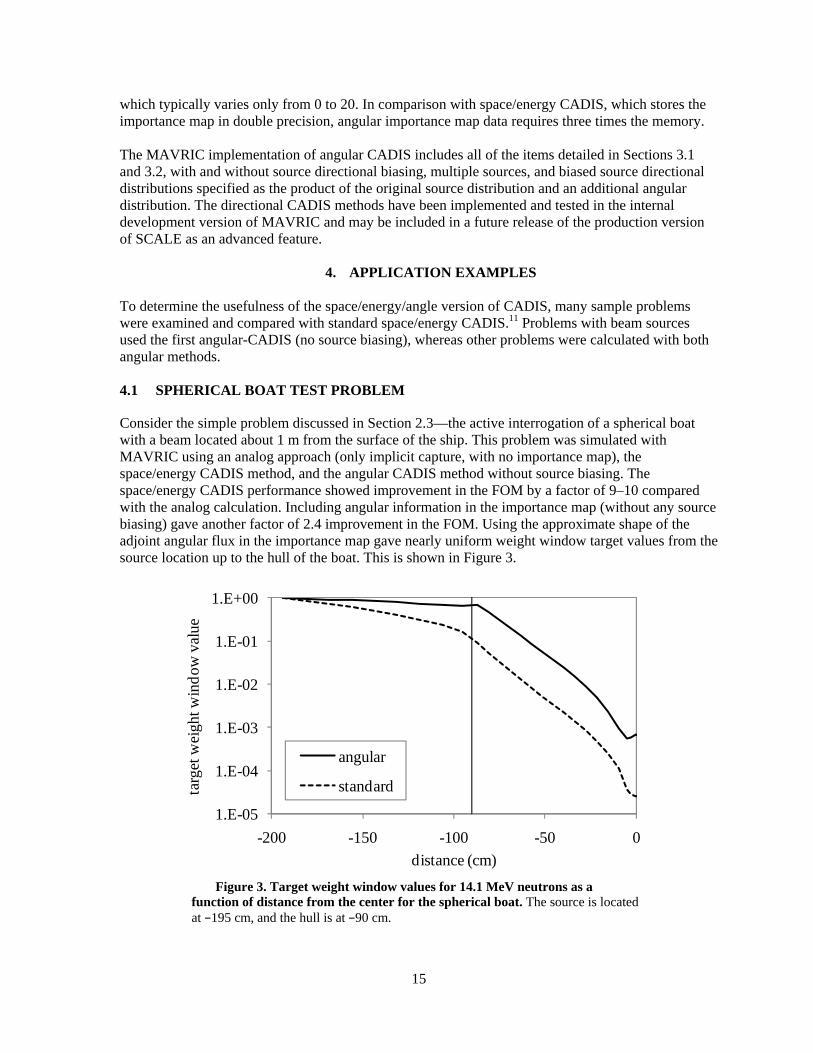
Consider the simple problem discussed in Section 2.3—the active interrogation of a spherical boat with a beam located about 1 m from the surface of the ship. This problem was simulated with MAVRIC using an analog approach (only implicit capture, with no importance map), the space/energy CADIS method, and the angular CADIS method without source biasing. The space/energy CADIS performance showed improvement in the FOM by a factor of 9–10 compared with the analog calculation. Including angular information in the importance map (without any source biasing) gave another factor of 2.4 improvement in the FOM. Using the approximate shape of the adjoint angular flux in the importance map gave nearly uniform weight window target values from the source location up to the hull of the boat. This is shown in Figure 3.

Figure 3. Target weight window values for 14.1 MeV neutrons as a function of distance from the center for the spherical boat. The source is located at −195 cm, and the hull is at −90 cm.

1.E-05

1.E-04

1.E-03

1.E-02

1.E-01

1.E+00

-200 -150 -100 -50 0

targ

et w

eigh

t win

dow

val

ue

distance (cm)

angular

standard

16

When the source position of the simple spherical boat problem was moved out to a distance of 10 m from the center of the boat, angular CADIS performed better than standard CADIS by a factor of 3.6, but both standard CADIS and angular CADIS calculations underperformed compared with the analog calculation. Ray effects were noticeable in the scalar adjoint, even at higher quadrature orders, because the true source was far from the adjoint source (center of the boat) and approximated a point source. The P1-type approximation used to model the directional component of the adjoint flux was not sufficient to provide uniform target weight windows between the source location and the hull of the boat. Both of the CADIS methods then had source particles with weight 1 having their first interaction in the hull of the boat where the target weight was ~1×10−4, as shown in Figure 4; this caused substantial splitting. The source sampling rate was then too low, which caused large uncertainties in the final result.

Figure 4. Target weight window values for 14.1 MeV neutrons as a function of distance from the center for the spherical boat. The source is located at −1025 cm, and the hull is at −90 cm.

A simpler way to improve this problem would be to use standard CADIS and then manually adjust the importance map so that the target weight window is 1 where the beam intersects the hull of the boat. This gives a factor of about 20 improvement over analog, far better than angular CADIS. The MAVRIC sequence in SCALE 6.1 contains an option, specifically designed for beam-in-air problems, that allows the user to change the point where the biased source and weight window map are normalized. Source particles are sampled, but their weights are not checked after birth. Particles typically do not interact in the air and arrive in the first non-air material with a weight that matches the weight window. 4.2 SIMPLE DUCT STREAMING PROBLEM

For an example of a duct streaming problem, consider a simple three-leg duct through a concrete parallelpiped, similar to that used by Sweezy et al.12 The concrete block is 150 cm high and wide and 100 cm deep. In the thinnest dimension of the block is a 10 cm diameter hole that includes two 90° turns and runs a total length of 160 cm. At the entrance of the duct is a point neutron source emitting a Watt spectrum. The objective is to calculate the total dose rate 10 cm from the duct exit.

1.E-08

1.E-06

1.E-04

1.E-02

1.E+00

-1200 -1000 -800 -600 -400 -200 0

targ

et w

eigh

t win

dow

val

ue

distance (cm)

angular

standard

17

Analog calculations for this problem are extremely slow to converge. Using standard space/energy CADIS is still slow but is 370 times faster than analog. The target weight values for the 0.9–1.4 MeV group are shown in Figure 5. Notice that these target weights range over 22 orders of magnitude, illustrating how difficult this “simple” problem is. Using the angular CADIS with source biasing, another factor of 2 can be gained. In this case, angular CADIS created a biased source using an exponential distribution with = 2.1, which samples many more neutrons in directions toward the first turn of the duct. The results are summarized in Table 1.

Figure 5. Duct streaming problem target weight values for the 0.9–1.4 MeV group. The source is at the lower left duct entrance, and the dose rate is calculated at the exit duct on the upper right.

Table 1. Results for a simple duct streaming problem

Calculation

SN time (min)

MC time (min)

Dose rate (rem/h)

Relative uncertainty

Monte Carlo FOM

Analog 1082 4.65×10–14 16.4% 0.0341 Standard CADIS 9.9 1084 5.04×10–14 0.855% 12.6 Angular CADIS 9.7 1081 5.02×10–14 0.602% 25.5

4.3 UEKI SHIELDING PROBLEM

Many measurements of different shielding materials were made by the Nuclear Technology Division of the Ship Research Institute in Japan by Ueki. A 252Cf source was placed at the center of a paraffin block with a cone cutout. The total neutron dose was measured behind graphite sheets of various thicknesses. The attenuation of the material was computed by comparing these measurements with a

18

measurement performed without any shield. Two of these measurements with graphite13 were simulated here using analog MC, space/energy CADIS, and space/energy/angle CADIS. For a 20 cm thick sheet of graphite, space/energy CADIS was about 50 times faster (FOM improvement) than the analog calculation. Angular CADIS without any source direction biasing was 1.5 to 2.2 times faster, depending on the specific energy (1 to 15 MeV) used to normalize the biased source and importance map. Angular CADIS with source directional biasing was a factor of 2.5 faster compared with the space/energy CADIS. This improvement was fairly independent of the energy used to normalize the biased source and importance map. For the 35 cm thick sheet, standard CADIS was 75 times faster than the analog calculation. Angular CADIS with source biasing was another factor of 2.1–2.6 times faster than standard CADIS. 4.4 NEUTRON WELL-LOGGING PROBLEM

A neutron porosity tool problem used in a previous study14 is based on an MCNP sample problem and was simulated using both space/energy CADIS and space/energy/angle CADIS. The model consists of an iron tool containing two detectors and a source placed in a water-filled hole in a homogenous limestone formation. The detectors are different distances from the source, which emits a spectrum of 0 to 11 MeV neutrons, preferentially in the direction of the two detectors. The total number of the 3He(n,p)3H interactions was computed for each detector. For both detectors, both versions of angular CADIS (with and without source directional biasing) were slightly (up to 10%) slower than the standard space/energy CADIS. In these cases, the parameter near the source and detectors was 2 or less (even lower when biasing for the far detector), showing that angular importance was not a strong factor. The extra overhead in computing and checking the angular target weight windows reduced the MC FOM more than the angular information helped. 4.5 GAMMA-RAY WELL-LOGGING PROBLEM

A gamma-ray litho-density tool, also used in the same study, was simulated using the new angular-based CADIS method. The model is based on a benchmark described by Gardner and Verghese.15 This tool contains two NaI detectors and an isotropic 137Cs source that is collimated to direct the photons into the formation and not directly at the detectors. The detectors are collimated to view the formation but not the source. This problem is generally harder to simulate than neutron tools, because the relatively low-energy photons have a more difficult time moving through the rock formation. The total photon flux was computed in each detector. For the near detector, angular CADIS reduces the Monte Carlo FOM from the standard CADIS by a factor of 4.6 and 3.4, for calculations with and without source biasing, respectively. For the far detector, angular CADIS results show a factor of 2 improvement over those from standard CADIS, with or without source biasing. For the near detector, it might be that the P1-type approximation of the directional importance is not close enough to the true directional importance, and as a result this type of biasing spent more time on particles going in unimportant directions. 4.6 ACTIVE INTERROGATION BARREL PROBLEM

As an example of a simple active interrogation system, consider the 55-gallon barrel scanner in Figure 6. A 14.1-MeV isotropic source and a helium-filled detector sit on opposite sides of the barrel. The goal is to compute the difference in detector signal between two water-filled barrels, one of

19

which also contains 25 kg of HEU (an International Atomic Energy Agency significant quantity). A two-step calculation is done for the barrel containing HEU, because particles can arrive at the detector from either the interrogation source or from fission induced in the HEU. For the first step, the simulation is optimized for finding the fission rate in the target material. A mesh tally over the target material from this step is then converted into a source for the second step. The second step is then optimized for finding the detector response from both the original source and the target material.

Figure 6. Interrogation geometry for a barrel (57 cm diam, 85 cm high), with a source (S) on the left side and a detector (D) on the right. The 25 kg sphere of HEU sits at the bottom of the barrel.

Standard space/energy CADIS speeds up both steps in this problem dramatically, with an overall improvement of about 390 for the whole two-step CADIS method compared with a single analog calculation of a barrel containing HEU.16,17 Angular CADIS, with and without source biasing, was applied to both steps of this problem. For calculating the fission source induced by the interrogation neutrons, angular CADIS without source biasing was three times faster than CADIS; with source biasing, it was 3.3 times faster than standard CADIS. For the second step (calculating the detector response to both sources), without source biasing it gave an improvement of 2 and with source biasing it gave an improvement of 1.7 over standard CADIS. 4.7 CARGO CONTAINER B PROBLEM

Another active interrogation system using an isotropic 2H–2H source (2.45 MeV neutrons) and a high-purity germanium photon detector for sealand cargo containers was also investigated. The model included a 12 m (40 ft) sealand cargo container, filled with a homogenous H/C/O/Fe mixture of

20

density 0.4 g/cm3, a detector on one side, and the source on the opposite side. In the center of the container was 25 kg of HEU. As shown in Figure 7, the container and detector were positioned 1 m over a concrete roadbed.

Figure 7. A 12 m (40 ft) sealand cargo container 1 m above a concrete roadbed with a detector (D) in the foreground and source on opposite side.

Similar to the 55-gallon barrel active interrogation problem, this problem requires calculations without the HEU and then multiple steps with the HEU. Because the difference between the detector count rates with and without the HEU is small (a few percent), a calculation can be made for just the detector response due to only the HEU fission photons and fission neutrons that generate photons through (n, ) reactions. For the container without HEU, standard CADIS improved the FOM by a factor of 32 over analog. With the HEU, a two-step CADIS method (determining the fission source and then the detector response) was 20 times faster than a single-step analog calculation. Angular CADIS with source biasing was then applied to this problem. For the container without the HEU, the active background detector count rate found using angular CADIS had an FOM 3.3 times higher than standard CADIS. For the two-step calculation of the total detector response for a container with HEU, angular CADIS improved step 1 by 16% and step 2 by a factor of 3.1. For finding the detector response due to only the fission source, angular CADIS was 2.8 times faster than standard CADIS.

21

5. CONCLUSIONS

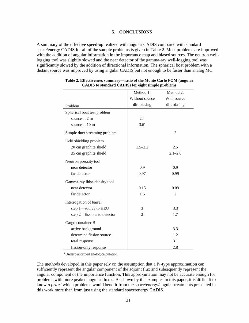
A summary of the effective speed-up realized with angular CADIS compared with standard space/energy CADIS for all of the sample problems is given in Table 2. Most problems are improved with the addition of angular information in the importance map and biased sources. The neutron well-logging tool was slightly slowed and the near detector of the gamma-ray well-logging tool was significantly slowed by the addition of directional information. The spherical boat problem with a distant source was improved by using angular CADIS but not enough to be faster than analog MC.

Table 2. Effectiveness summary—ratio of the Monte Carlo FOM (angular CADIS to standard CADIS) for eight simple problems

Method 1: Method 2:

Without source With source

Problem dir. biasing dir. biasing

Spherical boat test problem

source at 2 m 2.4

source at 10 m 3.6a

Simple duct streaming problem 2

Ueki shielding problem

20 cm graphite shield 1.5–2.2 2.5

35 cm graphite shield 2.1–2.6

Neutron porosity tool

near detector 0.9 0.9

far detector 0.97 0.99

Gamma-ray litho-density tool

near detector 0.15 0.09

far detector 1.6 2

Interrogation of barrel

step 1—source to HEU 3 3.3

step 2—fissions to detector 2 1.7

Cargo container B

active background 3.3

determine fission source 1.2

total response 3.1

fission-only response 2.8 aUnderperformed analog calculation

The methods developed in this paper rely on the assumption that a P1-type approximation can sufficiently represent the angular component of the adjoint flux and subsequently represent the angular component of the importance function. This approximation may not be accurate enough for problems with more peaked angular fluxes. As shown by the examples in this paper, it is difficult to know a priori which problems would benefit from the space/energy/angular treatments presented in this work more than from just using the standard space/energy CADIS.

22

Another consequence of using a P1-type approximation to represent the angular adjoint flux is that a different normalization of the biased source(s) and the target weight windows is required. In space/energy CADIS, the target weights and the source birth weights match for all source particles. In the two approaches presented in this paper, the source birth weights at each source match only the target weight windows at one specific point in the space/energy/angle phase space. For sources that are small compared with the problem size, birth weights for source particles not born at that specific point will still be close to the target weight windows where they were born. Selecting the appropriate point in phase space for each of the sources requires some thought and input from the user. Because using the complete angular information from the deterministic adjoint calculation would require large amounts of memory and would be difficult for the MC code, a potential improvement on the approaches detailed in this paper would be to develop the space/energy weight windows using forward deterministic calculations that include the directional information of particles within a given space-energy cell. Then, instead of computing a space/energy importance based on the scalar adjoint flux (equivalent to integrating the angular adjoint flux with an isotropic weighting function), the forward flux estimate could be used to collapse the angular adjoint flux into a space/energy importance that represents the particles that actually move through that cell. A deterministic solution is needed to calculate what the MCNP weight window generator computes—space/energy weight targets for particles traveling in the specific directions at those locations that the MC will simulate. With a deterministic solution, both the problem of zero scores far from the source and the overall iterative nature of the weight window generator are avoided.

23

6. REFERENCES

1. J. C. Wagner and A. Haghighat, “Automated Variance Reduction of Monte Carlo Shielding

Calculations Using the Discrete Ordinates Adjoint Function,” Nuclear Science & Engineering 128, 186 (1998).

2. D. E. Peplow, T. M. Evans, and J. C. Wagner, “Simultaneous Optimization of Tallies in Difficult Shielding Problems,” Nuclear Technology 168(3), 785–792 (2009).

3. A. Haghighat and J. C. Wagner, “Monte Carlo Variance Reduction with Deterministic Importance Functions,” Progress in Nuclear Energy 42(1), 25–53 (2003).

4. S. W. Mosher, T. M. Miller, T. M. Evans, and J. C. Wagner, “Automated Weight-Window Generation for Threat Detection Applications using ADVANTG,” Proceedings of the 2009 International Conference on Advances in Mathematics, Computational Methods, and Reactor Physics (M&C 2009), Saratoga Springs, NY, May 3–7, 2009, on CD-ROM, American Nuclear Society, LaGrange Park, IL (2009).

5. X-5 MONTE CARLO TEAM, MCNP – A General Monte Carlo N-Particle Transport Code, Version 5—Volume II: User’s Guide, LA-CP-03-0245, Los Alamos National Laboratory (2008).

6. D. E. Peplow, “Monte Carlo Shielding Analysis Capabilities with MAVRIC,” Nuclear

Technology 174, 289–313 (2011).

7. SCALE: A Comprehensive Modeling and Simulation Suite for Nuclear Safety Analysis and Design, ORNL/TM-2005/39, Version 6.1, June 2011. Available from Radiation Safety Information Computational Center at Oak Ridge National Laboratory as CCC-785.

8. T. M. Evans, A. S. Stafford, and K. T. Clarno, “Denovo—A New Three-Dimensional Parallel Discrete Ordinates Code in SCALE,” Nuclear Technology 171, 171–200 (2010).

9. K. A. Van Riper, T. J. Urbatsch, P. D. Soran, D. K. Parsons, J. E. Morel, G. W. McKinney, S. R. Lee, L. A. Crotzer, F. W. Brinkley, T. E. Booth, J. W. Anderson, and R. E. Alcouffe, “AVATAR— Automatic Variance Reduction in Monte Carlo Calculations,” Proceedings of the Joint International Conference on Mathematical Methods and Supercomputing in Nuclear Applications 1, Saratoga Springs, New York (October 6–10, 1997), p. 661 (1997).

10. T. M. Evans and J. S. Hendricks, “An Enhanced Geometry-Independent Mesh Weight Window Generator for MCNP,” Proceedings of the 1998 ANS Radiation Protection and Shielding Division Topical Conference 1, p. 165, Nashville, TN, April 19–23, 1998.

11. D. E. Peplow, S. W. Mosher, and T. M. Evans, “Hybrid Monte Carlo/Deterministic Methods for Streaming/Beam Problems,” Book of Abstracts, American Nuclear Society Joint Topical Meeting of the Radiation Protection and Shielding Division Isotopes and Radiation Division, and Biology and Medicine Division Las Vegas, NV, April 18–23, 2010.

12. J. Sweezy, F. Brown, T. Booth, J. Chiaramonte, and B. Preeg, “Automated Variance Reduction For MCNP Using Deterministic Methods,” Radiation Protection Dosimetry 116(1–4), 508–512 (2005).

24

13. K. Ueki, A. Ohashi, N. Nariyama, S. Nagayama, T. Fujita, K. Hattori and Y. Anayama,

“Systematic Evaluation of Neutron Shielding Effects for Materials,” Nuclear Science and Engineering 124, 455-464 (1996).

14. J. C. Wagner, D. E. Peplow, and T. M. Evans, “Automated Variance Reduction Applied to Nuclear Well-Logging Problems,” Nuclear Technology 168(3), 799-809 (2009).

15. R. P. Gardner and K. Verghese, “Monte Carlo Nuclear Well Logging Benchmark Problems with Preliminary Intercomparison Results,” Nuclear Geophysics 5(4), 429–438 (1991).

16. D. E. Peplow, T. M. Miller, and B. W. Patton, “Hybrid Monte Carlo/Deterministic Methods for Active Interrogation Modeling,” Book of Abstracts, American Nuclear Society Joint Topical Meeting of the Radiation Protection and Shielding Division, Isotopes and Radiation Division, and Biology and Medicine Division Las Vegas, NV, April 18-23, 2010.

17. D. E. Peplow, T. M. Miller, B. W. Patton, and J. C. Wagner, “Hybrid Monte Carlo/Deterministic Methods for Active Interrogation Modeling,” accepted for publication by Nuclear Technology (2012).