Prepared for submission to JCAP

Conservative Constraints on EarlyCosmology: an illustration of theMonte Python cosmologicalparameter inference code

Benjamin Audren,a Julien Lesgourgues,a,b,c Karim Benabed,dand Simon Prunetd

aInstitut de Théorie des Phénomènes Physiques,École Polytechnique Fédérale de Lausanne,CH-1015, Lausanne, SwitzerlandbCERN, Theory Division,CH-1211 Geneva 23, SwitzerlandcLAPTh (CNRS -Université de Savoie), BP 110,F-74941 Annecy-le-Vieux Cedex, FrancedInstitute d’Astrophysique de Paris, 98 Bd Arago, F-75014 Paris, France

E-mail: benjamin.audren@epfl.ch, Julien.Lesgourgues@cern.ch, benabed@iap.fr,prunet@iap.fr

Abstract. Models for the latest stages of the cosmological evolution rely on a less solidtheoretical and observational ground than the description of earlier stages like BBN andrecombination. As suggested in a previous work by Vonlanthen et al., it is possible to tweakthe analysis of CMB data in such way to avoid making assumptions on the late evolution,and obtain robust constraints on “early cosmology parameters”. We extend this method inorder to marginalise the results over CMB lensing contamination, and present updated resultsbased on recent CMB data. Our constraints on the minimal early cosmology model are weakerthan in a standard ΛCDM analysis, but do not conflict with this model. Besides, we obtainconservative bounds on the effective neutrino number and neutrino mass, showing no hints forextra relativistic degrees of freedom, and proving in a robust way that neutrinos experiencedtheir non-relativistic transition after the time of photon decoupling. This analysis is also anoccasion to describe the main features of the new parameter inference code Monte Python,that we release together with this paper. Monte Python is a user-friendly alternative toother public codes like CosmoMC, interfaced with the Boltzmann code class.

arX

iv:1

210.

7183

v2 [

astr

o-ph

.CO

] 3

1 O

ct 2

012

Contents

1 Introduction 1

2 How to test early cosmology only? 2

3 Results assuming a minimal early cosmology model 5

4 Effective neutrino number and neutrino mass 8

5 Advantages of Monte Python 12

6 Conclusions 16

1 Introduction

Models for the evolution of the early universe between a redshift of a few millions and afew hundreds have shown to be very predictive and successful: the self-consistency of BigBang Nucleosynthesis (BBN) model could be tested by comparing the abundance of lightelements and the result of Cosmic Microwave Background (CMB) observations concerning thecomposition of the early universe; the shape of CMB acoustic peaks matches accurately theprediction of cosmological perturbation theory in a Friedmann-Lemaître Universe describedby general relativity, with a thermal history described by standard recombination. The latecosmological evolution is more problematic. Models for the acceleration of the universe,based on a cosmological constant, or a dark energy component, or departures from generalrelativity, or finally departure from the Friedmann-Lemaître model at late times, have shownno predictive power so far. The late thermal history, featuring reionization from stars, isdifficult to test with precision. Overall, it is fair to say that “late cosmology” relies on lesssolid theoretical or observational ground than “early cosmology”.

When fitting the spectrum of temperature and polarisation CMB anisotropies, we makesimultaneously some assumptions on early and late cosmology, and obtain intricate constraintson the two stages. However, Vonlanthen et al. [1] suggested a way to carry the analysis leadingto constraints only on the early cosmology part. This is certainly interesting since such ananalysis leads to more robust and model-indepent bounds than a traditional analysis affectedby priors on the stages which are most poorly understood. The approach of [1] avoids makingassumptions on most relevant “late cosmology-related effects”: projection effects due to thebackground evolution, photon rescattering during reionization, and the late Integrated SachsWolfe (ISW) effect.

In this work, we carry a similar analysis, pushed to a higher precision level since wealso avoid making assumptions on the contamination of primary CMB anisotropies by weaklensing. We use the most recent available data from the Wilkinson Microwave AnisotropyProbe (WMAP) and South Pole Telescope (SPT) data, and consider the case of a minimal“early cosmology” model, as well as extended models with free density of ultra-relativisticrelics or massive neutrinos.

This analysis is an occasion to present a new cosmological parameter inference code. ThisMonte Carlo code written in Python, called Monte Python1, offers a convenient alternative

1http://montepython.net

– 1 –

to CosmoMC [4]. It is interfaced with the Boltzmann code class2 [2, 3]. Monte Pythonis released publicly together with this work.

In section 2, we explain the method allowing to get constraints only on the early cos-mological evolution. We present our result for the minimal early cosmology model in section3, and for two extended models in section 4. In section 5, we briefly summarize some of theadvantages of Monte Pyhton, without entering into technical details (presented anyway inthe code documentation). Our conclusions are highlighted in section 6.

2 How to test early cosmology only?

The spectrum of primary CMB temperature anisotropies is sensitive to various physical effects:

• (C1) the location of the acoustic peaks in multipole space depends on the sound horizonat decoupling ds(τrec) (an “early cosmology”-dependent parameter) divided by the angu-lar diameter distance to decoupling dA(τrec) (a “late cosmology”-dependent parameter,sensitive to the recent background evolution: acceleration, spatial curvature, etc.)

• (C2) the contrast between odd and even peaks depends on ωb/ωγ , i.e. on “early cosmol-ogy”.

• (C3) the amplitude of all peaks further depends on the amount of expansion betweenradiation-to-matter equality and decoupling, governing the amount of perturbationdamping at the beginning of matter domination, and on the amount of early inte-grated Sachs-Wolfe effect enhancing the first peak just after decoupling. These areagain “early cosmology” effects (in the minimal ΛCDM model, they are both regulatedby the redshift of radiation-to-matter equality, i.e by ωm/ωr).

• (C4) the enveloppe of high-` peaks depends on the diffusion damping scale at decou-pling λd(τrec) (an “early cosmology” parameter) divided again by the angular diameterdistance to decoupling dA(τrec) (a “late cosmology” parameter).

• (C5-C6) the global shape depends on initial conditions through the primordial spectrumamplitude As (C5) and tilt ns (C6), which are both “early cosmology” parameters.

• (C7) the slope of the temperature spectrum at low ` is affected by the late integratedSachs Wolfe effect, i.e. by “late cosmology”. This effect could actually be consideredas a contamination of the primary spectrum by secondary anisotropies, which are notbeing discussed in this list.

• (C8) the global amplitude of the spectrum at ` 40 is reduced by the late reionizationof the universe, another “late cosmology” effect. The amplitude of this suppression isgiven by e−2τ , where τ is the reionization optical depth.

In summary, primary CMB temperature anisotropies are affected by late cosmology onlythrough: (i) projection effects from real space to harmonic space, controlled by dA(τrec); (ii)the late ISW effect, affecting only small `’s; and (iii) reionization, suppressing equally allmultipoles at ` 40 . These are actually the sectors of the cosmological model which aremost poorly constrained and understood. But we see that the shape of the power spectrum

2http://class-code.net

– 2 –

0

1

2

3

4

5

6

7

8

9

10 100 1000

l(l+

1)C

lTT / 2

π (x

10

10)

l

10-16

10-15

10-14

10-13

10-12

10-11

10 100 1000

l(l+

1)C

lEE / 2

π

l

Figure 1. Dimensionless temperature (left) and E-polarization (right) unlensed spectra of two ΛCDMmodels with the same value of “early cosmology” parameters (ωb, ωcdm, As, ns) (fixed to WMAP best-fitting values), and different values of “late cosmology” parameters: (ΩΛ, zreio) = (0.720,10) (solidcurves) or (0.619, 5) (dashed curve). The dashed curves have been rescaled vertically by the ratioof e−2τ and horizontally by the ratio of dA(τrec) in each model, using the values of τ and dA(τrec)calculated by class for each model. At ` = 40, the difference between the dashed and solid line inthe temperature plot is under 2µK2. At ` = 80, it is already below 1µK2.

at ` 40, interpreted modulo an arbitrary scaling in amplitude (C` → αC`) and in position(C` → Cβ`), contains information on early cosmology only. This statement is very generaland valid for extended cosmological models. In the case of the ΛCDM models, it is illustratedby figure 1, in which we took two different ΛCDM models (with different late-time geometryand reionization history), and rescaled one of them with a shift in amplitude given by e−2τ−τ ′

and in scale given by dA/d′A. At ` 40, the two spectra are identical. For more complicatedcosmological models sharing the same physical evolution until approximately z ∼ 100, asimilar rescaling and matching would work equally well.

If polarization is taken into account, the same statement remains valid. The late timeevolution affects the polarization spectrum through the angular diameter distance to de-coupling dA(τrec) and through the impact of reionization, which also suppresses the globalamplitude at ` 40, and generates an additional feature at low `’s, due to photon re-scateringby the inhomogeneous and ionized inter-galactic medium. The shape of the primary temper-ature and polarization spectrum at ` 40, interpreted modulo a global scaling in amplitudeand in position, only contains information on the early cosmology.

However, the CMB spectrum that we observe today gets a contribution from secondaryanisotropies and foregrounds. In particular, the observed CMB spectra are significantly af-fected by CMB lensing caused by large scale structures. This effect depends on the small scalematter power spectrum, and therefore on late cosmology (acceleration, curvature, neutrinosbecoming non-relativistic at late time, possible dark energy perturbations, possible departuresfrom Einstein gravity on very large scales, etc.). In the work of [1], this effect was mentionedbut not dealt with, because of the limited precision of WMAP5 and ACBAR data comparedto the amplitude of lensing effects, at least within the multipole range studied in that pa-per (40 ≤ ` ≤ 800). The results that we will present later confirm that this simplification

– 3 –

was sufficient and did not introduce a significant “late cosmology bias”. However, with thefull WMAP7+SPT data (that we wish to use up to the high multipoles), it is not possibleto ignore lensing, and in order to probe only early cosmology, we are forced to marginalizeover the lensing contamination, in the sense of the method described below. By doing so,we will effectively get rid of the major two sources of secondary (CMB) anisotropies, thelate ISW effect and CMB lensing. We neglect the impact of other secondary effects like theRees-Sciama effect. As far as foregrounds are concerned, the approach of WMAP and SPTconsists in eliminating them with a spectral analysis, apart from residual foregrounds whichcan be fitted to the data, using some nuisance parameters which are marginalized over. Byfollowing this approach, we also avoid to introduce a “late cosmology bias” at the level offoregrounds.

Let us now discuss how one can marginalize over lensing corrections. Ideally, we shouldlens the primary CMB spectrum with all possible lensing patterns, and marginalize over theparameters describing these patterns. But the lensing of the CMB depends on the lensingpotential spectrum Cφφ` , that can be inferred from the matter power spectrum at small red-shift, P (k, z). We should marginalize over all possible shapes for Cφφ` , i.e. over an infinity ofdegrees of freedom. We need to find a simpler approach.

One can start by noticing that modifications of the late-time background evolutioncaused by a cosmological constant, a spatial curvature, or even some inhomogeneous cos-mology models, tend to affect matter density fluctuations in a democratic way: all Fouriermodes being inside the Hubble radius and on linear scales are multiplied by the same redshift-dependent growth factor. CMB lensing is precisely caused by such modes. Hence, for thiscategory of models, differences in the late-time background evolution lead to a different am-plitude for Cφφ` , and also a small tilt since different `’s probe the matter power spectrum atdifferent redshifts. Hence, if we fit the temperature and polarization spectrum at ` 40modulo a global scaling in amplitude, a global shift in position, and additionally an arbitraryscaling and tilting of the lensing spectrum Cφφ` that one would infer assuming ΛCDM, westill avoid making assumption about the late-time evolution.

There are also models introducing a scale-dependent growth factor, i.e. distortions inthe shape of the matter power spectrum. This is the case in presence of massive neutrinosor another hot dark matter component, of dark energy with unusually large perturbationscontributing to the total perturbed energy-momentum tensor, or in modified gravity models.In principle, these effects could lead to arbitrary distortions of Cφφ` as a function of `. For-tunately, CMB lensing only depends on the matter power spectrum P (k, z) integrated overa small range of redshifts and wave numbers. Hence it makes sense to stick to an expansionscheme: at first order we can account for the effects of a scale-dependent growth factor bywriting the power spectrum as the one predicted by ΛCDM cosmology, multiplied by arbi-trary rescaling and tilting factors; and at the next order, one should introduce a running ofthe tilt, then a running of the running, etc. By marginalizing over the rescaling factor, tiltingfactor, running, etc., one can still fit the CMB spectra without making explicit assumptionsabout the late-time cosmology. In the result section, we will check that the information onearly cosmology parameters varies very little when we omit to marginalize over the lensingamplitude, or when we include this effect, or when we also marginalize over a tilting factor.Hence we will not push the analysis to the level of an arbitrary lensing running factor.

– 4 –

3 Results assuming a minimal early cosmology model

We assume a “minimal early cosmology” model described by four parameters (ωb, ωcdm, As,ns). In order to extract constraints independent of the late cosmological evolution, we needto fit the CMB temperature/polarisation spectrum measured by WMAP (seven year data [5])and SPT [6] only above a given value of ` (typically ` ∼ 40), and to marginalize over twofactors accounting for vertical and a horizontal scaling. In practice, there are several ways inwhich this could be implemented.

For the amplitude, we could fix the reionization history and simply marginalize overthe amplitude parameter As. By fitting the data at ` 40, we actually constrain theproduct e−2τreioAs, i.e. the primordial amplitude rescaled by the reionization optical depthτreio, independently of the details of reionization. In our runs, we fix τreio to an arbitraryvalue, and we vary As; but in the Markov chains, we keep memory of the value of the derivedparameter e−2τreioAs. By quoting bounds on e−2τAs rather than As, we avoid making explicitassumptions concerning the reionization history.

For the horizontal scaling, we could modify class in such way to use directly dA(τrec)as an input parameter. For input values of (ωb, ωcdm, dA(τrec)), class could in principlefind the correct spectrum at ` 40. It is however much simpler to use the unmodified codeand pass values of the five parameters (ωb, ωcdm, As, ns, h). In our case, h should not beinterpreted as the reduced Hubble rate, but simply as a parameter controlling the value ofthe physical quantity dA(τrec). For any given set of parameters, the code computes the valuethat dA(τrec) would take in a ΛCDM model with the same early cosmology and with a Hubblerate H0 = 100hkm/s/Mpc. It then fits the theoretical spectrum to the data. The resultinglikelihood should be associated to the inferred value of dA(τrec) rather than to h. The onlydifference between this simplified approach and that in which dA(τrec) would be passed as aninput parameter is that in one case, one assumes a flat prior on dA(τrec), and in the other casea flat prior on h. But given that the data allows dA(τrec) to vary only within a very smallrange where it is almost a linear function of h, the prior difference has a negligible impact.

To summarize, in order to get constraints on “minimal early cosmology”, it is sufficientto run Markov Chains in the same way as for a minimal ΛCDM model with parameters (ωb,ωcdm, As, ns, τ , h), excepted that:

• we do not fit the lowest temperature/polarization multipoles to the data;

• we fix τ to an arbitrary value;

• we do not plot nor interpret the posterior probability of the parameters As and h. Weonly pay attention to the posterior probability of the two derived parameters e−2τAsand dA(τrec), which play the role of the vertical and horizontal scaling factors, and whichare marginalized over when quoting bounds on the remaining three “early cosmologyparameters” (ωb, ωcdm, ns).

Hence, for a parameter inference code, this is just a trivial matter of defining and storingtwo “derived parameters”. For clarity, we will refer to the runs performed in this way as the“agnostic” runs.

In the second line of Table 1, we show the bounds obtained with such an agnostic run, fora cut-off value ` = 40. These results can be compared with those of a minimal ΛCDM model,obtained through the same machinery but with all multipoles ` ≥ 2. Since the agnostic boundsrely on less theoretical assumptions, they are slightly wider. Interestingly, the central value of

– 5 –

100 ωb ωcdm ns dArec 109e−2τAs Alp nlp

ΛCDM

2.241+0.043−0.044 0.1114+0.0048

−0.0048 0.960+0.011−0.011 12.93+0.11

−0.12 2.069+0.085−0.092

same lensing potential as in ΛCDM

` ≥ 40 2.204+0.048−0.047 0.1160+0.0056

−0.0059 0.946+0.014−0.014 12.85+0.13

−0.13 2.20+0.12−0.13

` ≥ 60 2.203+0.050−0.053 0.1163+0.0063

−0.0065 0.945+0.016−0.016 12.84+0.14

−0.14 2.20+0.13−0.15

` ≥ 80 2.190+0.053−0.057 0.1180+0.0067

−0.0073 0.940+0.019−0.018 12.81+0.15

−0.15 2.26+0.15−0.18

` ≥ 100 2.184+0.054−0.056 0.1187+0.0067

−0.0079 0.935+0.020−0.019 12.80+0.16

−0.15 2.29+0.16−0.20

marginalization over lensing potential amplitude

` ≥ 100 2.159+0.060−0.064 0.1227+0.0083

−0.0088 0.926+0.022−0.022 12.73+0.18

−0.17 2.39+0.20−0.23 0.88+0.12

−0.13

marginalization over lensing potential amplitude and tilt

` ≥ 100 2.160+0.064−0.068 0.1222+0.0088

−0.0094 0.927+0.024−0.024 12.74+0.18

−0.18 2.38+0.20−0.25 0.78+0.20

−0.15 −0.16+0.55−0.33

Table 1. Limits at the 68% confidence level of the mininum credible interval of model parameters.The ΛCDM model of the first line has a sixth independent parameter (zreio) that we do not show.We do not show either the limits on the three nuisance parameters associated to the SPT likelihood.

ωb and ns are smaller in absence of late-cosmology priors, and larger for ωcdm. Still the ΛCDMresults are compatible with the agnostic results, which means that on the basis of this test,we cannot say that ΛCDM is a bad model. Our agnostic bounds on (ωb, ωcdm, ns) are simplymore model-independent and robust, and one could argue that when using CMB bounds inthe study of BBN, in CDM relic density calculations or for inflationary model building, oneshould better use those bounds in order to avoid relying on the most uncertain assumptionsof the minimal cosmological model, namely Λ domination and standard reionization.

The decision to cut the likelihood at ` ≥ 40 was somewhat arbitrary. Figure 1 showsthat two rescaled temperature spectra with different late-time cosmology tend only graduallytowards each other above ` ∼ 40. We should remove enough low multipoles in order to besure that late time cosmology has a negligible impact given the data error bars. We testedthis dependence by cutting the likelihood at ` ≥ 60, ` ≥ 80 or ` ≥ 100. When increasingthe cut-off from 40 to 100, we observe variations in the mean value that are less importantthan from 2 to 40. To have the more robust constraints, we will then take systematically thecut-off of ` = 100, which is the one more likely to avoid any contamination from “late timecosmology”.

Until now, our analysis is not completely “agnostic”, because we did not marginalizeover lensing. We fitted the data with a lensed power spectrum, relying on the same lensingpotential as an equivalent ΛCDM model with the same values of (ωb, ωcdm, ns, e−2τAs,dA(τrec)). To deal with lensing, we introduce three new parameters (Alp, nlp, klp) in class.

– 6 –

1.975 2.186 2.407

100 ωb= 2.241+0.04342−0.04433

0.09602 0.1239 0.1518

ωcdm= 0.1114+0.004817−0.004845

0.8578 0.9275 0.9972

ns= 0.9603+0.01111−0.0111

6.386 10.62 14.86

zreio= 10.42+1.214−1.184

12.2 12.75 13.29

drecA = 12.93+0.1141−0.1226

1.827 2.484 3.141

10+9e−2τAs= 2.069+0.08513−0.0919

0.1 0.8046 1.366

Alp= 0.7803+0.204−0.1473

-1.426 -0.3551 1

nlp= −0.172+0.5596−0.3343

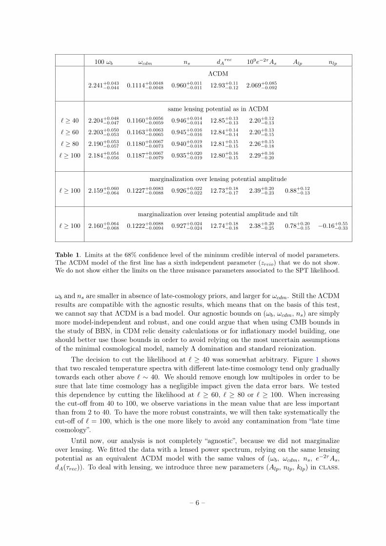
Figure 2. Constraints on the five parameters of the minimal early cosmology model (red), comparedto usual constraints on the minimal ΛCDM model (black). The ΛCDM has a sixth independentparameter, the reionization optical depth. The constraints on early cosmology (called “agnostic con-straints” in the text) includes a marginalization over the amplitude and tilt of the matter powerspectrum leading to CMB lensing. We do not show here the posterior of the three nuisance parameterused to fit SPT data.

Given the traditional input parameters (ωb, ωcdm, As, ns, h), the code first computes theNewtonian potential φ(k, z). This potential is then rescaled as

φ(k, z) −→ Alp

(k

klp

)nlp

φ(k, z) . (3.1)

Hence, the choice (Alp, nlp)=(1,0) corresponds to the standard lensing potential predicted inthe ΛCDMmodel. Different values correspond to an arbitrary rescaling or tilting of the lensingpotential, which can be propagated consistently to the lensed CMB temperature/polarizationspectrum.

The sixth run shown in Table 1 corresponds to nlp = 0 and a free parameter Alp.The minimum credible interval for this rescaling parameter is Alp = 0.88+0.12

−0.13 at the 68%Confidence Level (CL), and is compatible with one. This shows that WMAP7+SPT dataalone are sensitive to lensing, and well compatible with the lensing signal predicted by theminimal ΛCDM model. It is also interesting to note that the bounds on other cosmological

– 7 –

parameter move a little bit, but only by a small amount (compared to the difference betweenthe ΛCDM and the previous “agnostic” runs), showing that “agnostic bounds” are robust.

In the seventh line of Table 1, we also marginalize over the tilting parameter nlp (withunbounded flat prior). A priori, this introduces a lot of freedom in the model. Nicely, thisparameter is still well constrained by the data (nlp = −0.16+0.55

−0.33 at 68%CL), and compatiblewith the ΛCDM prediction nlp = 0. Bounds on other parameters vary this time by a com-pletely negligible amount: this motivates us to stop the expansion at the level of nlp, and notto test the impact of running. The credible interval for Alp is the only one varying signifi-cantly when nlp is left free, but this result depends on the pivot scale klp, that we choose tobe equal to klp = 0.1/Mpc, so that the amplitude of the lensing spectrum Cφφ` is nearly fixedat ` ∼ 100. By tuning the pivot scale, we could have obtained bounds on As nearly equalfor the case with/without free nlp. The posterior probability of each parameter marginalizedover other parameters is shown in Figure 2, and compared with the results of the standardΛCDM analysis.

Our results nicely agree with those of [1]. These authors found a more pronounceddrift of the parameters (ωb, ωcdm, ns) with the cut-off multipole than in the first part ofour analysis, but this is because we use data on a wider multipole range and have a largerlever arm. Indeed, Ref. [1] limited their analysis of WMAP5 plus ACBAR data to ` ≤ 800,arguing that above this value, lensing would start playing an important role. In our analysis,we include WMAP7 plus 47 SPT band powers probing up to ` ∼ 3000, but for consistency wemust simultaneously marginalize over lensing. Indeed, the results of Ref. [1] are closer to ourresults with lensing marginalization (the fully “agnostic” ones) that without. Keeping only onedigit in the error bar, we find (100ωb = 2.16± 0.07, ωcdm = 0.122± 0.009, ns = 0.93± 0.02),when this reference found (100ωb = 2.13 ± 0.05, ωcdm = 0.124 ± 0.007, ns = 0.93 ± 0.02).The two sets of results are very close to each other, but our central values for ωb and ωcdmare slightly closer to the ΛCDM one. The fact that we get slightly larger error bars in spiteof using better data in a wider multipole range is related to our lensing marginalization: wesee that by fixing lensing, this previous analysis was implicitly affected by a partial “latecosmology prior”, but only at a very small level.

Our results from the last run can be seen as robust “agnostic” bounds on (ωb, ωcdm, ns),only based on the “minimal early cosmology” assumption. They are approximately twice lessconstraining than ordinary ΛCDM models, and should be used in conservative studies of thephysics of BBN, CDM decoupling and inflation.

4 Effective neutrino number and neutrino mass

We can try to generalize our analysis to extended cosmological models. It would make nosense to look at models with spatial curvature, varying dark energy or late departures fromEinstein gravity, since all these assumptions would alter only the late time evolution, and ourmethod is designed precisely in such way that the results would remain identical. However, wecan explore models with less trivial assumptions concerning the early cosmological evolution.This includes for instance models with:

• a free primordial helium fraction YHe. So far, we assumed YHe to be a function ofωb, as predicted by standard BBN (this is implemented in class following the linesof Ref. [7]). Promoting YHe as a free parameter would be equivalent to relax theassumption of standard BBN. Given the relatively small sensitivity of current CMB

– 8 –

100 ωb ωcdm ns Neff dArec 109e−2τAs Alp nlp

ΛCDM

2.279+0.053−0.056 0.124+0.011

−0.013 0.979+0.019−0.019 3.77+0.58

−0.66 12.35+0.46−0.53 2.01+0.10

−0.10

` ≥ 100, marginalization over lensing potential amplitude and tilt

2.03+0.13−0.16 0.113+0.011

−0.015 0.862+0.065−0.077 2.04+0.78

−1.26 13.59+0.96−0.87 2.84+0.49

−0.59 0.69+0.21−0.18 −0.23+0.57

−0.43

Table 2. Limits at the 68% confidence level of the minimum credible interval of model parameters.The ΛCDM+Neff model of the first line has a seventh independent parameter (zreio) that we do notshow. We do not show either the limits on the three nuisance parameters associated to the SPTlikelihood.

data to YHe [5], we do not perform such an analysis here, but this could be done in thefuture using e.g. Planck data.

• a free density of relativistic species, parametrized by a free effective neutrino numberNeff , differing from its value of 3.046 in the minimal ΛCDM model [8]. This parameteraffects the time of equality between matter and radiation, but this effect can be cancelledat least at the level of “early cosmology” by tuning appropriately the density of baronsand CDM. Even in that case, relativistic species will leave a signature on the CMBspectrum, first through a change in the diffusion damping scale λd(τrec), and secondthrough direct effects at the level of perturbations, since they induce a gravitationaldamping and phase shifting of the photon fluctuation [9, 10]. It is not obvious toanticipate up to which level these effects are degenerate with those of other parameters.Hence it is interesting to run Markov chains and search for “agnostic bounds” on Neff .

• neutrino masses (or for simplicity, three degenerate masses mν summing up to Mν =3mν). Here we are not interested in the fact that massive neutrinos affect the back-ground evolution and change the ratio between the redshift of radiation-to-matter equal-ity, and that of matter-to-Λ equality. This is a “late cosmology” effect that we cannotprobe with our method, since we are not sensitive to the second equality. However, formasses of the order of mν ∼ 0.60 eV, neutrinos become non-relativistic at the time ofphoton decoupling. Even below this value, the mass leaves a signature on the CMBspectrum coming from the fact that, first, they are not yet ultra-relativistic at decou-pling, and second, the transition to the non-relativistic regime takes place when theCMB is still probing metric perturbations through the early integrated Sachs-Wolfe ef-fect. Published bounds on Mν from CMB data alone probe all these intricate effects[5], and it would be instructive to obtain robust bounds based only on the mass impacton “early cosmology”.

For the effective neutrino number, we performed two runs similar to our previous ΛCDMand “fully agnostic” run (with marginalization over lensing amplitude and tilt), in presenceof one additional free parameter Neff . Our results are summarized in Table 2 and Figure 3.In the ΛCDM+Neff case, we get Neff = 3.77+0.58

−0.66 (68% CL), very close to the result of [11],Neff = 3.85 ± 0.62 (differences in the priors can explain this insignificant difference). It

– 9 –

1.73 2.14 2.55

100 ωb= 2.03+0.13−0.164

0.0856 0.125 0.164

ωcdm= 0.113+0.0108−0.015

0.0856

0.125

0.164

0.726 0.893 1.06

ns= 0.862+0.0649−0.0771

0.726

0.893

1.06

0 3.31 5.91

Neff= 2.04+0.776−1.26

0

3.31

5.91

0 0.768 1.38

Alp= 0.686+0.21−0.179

0

0.768

1.38

-1.68 -0.499 1

nlp= −0.229+0.568−0.426

-1.68

-0.499

1

11.3 13.5 15.7

drecA = 13.6+0.959−0.874

11.3

13.5

15.7

1.74 3.04 4.34

10+9e−2τAs= 2.84+0.494−0.595

1.73 2.14 2.551.74

3.04

4.34

0.0856 0.125 0.164 0.726 0.893 1.06 0 3.31 5.91 0 0.768 1.38 -1.68 -0.499 1 11.3 13.5 15.7

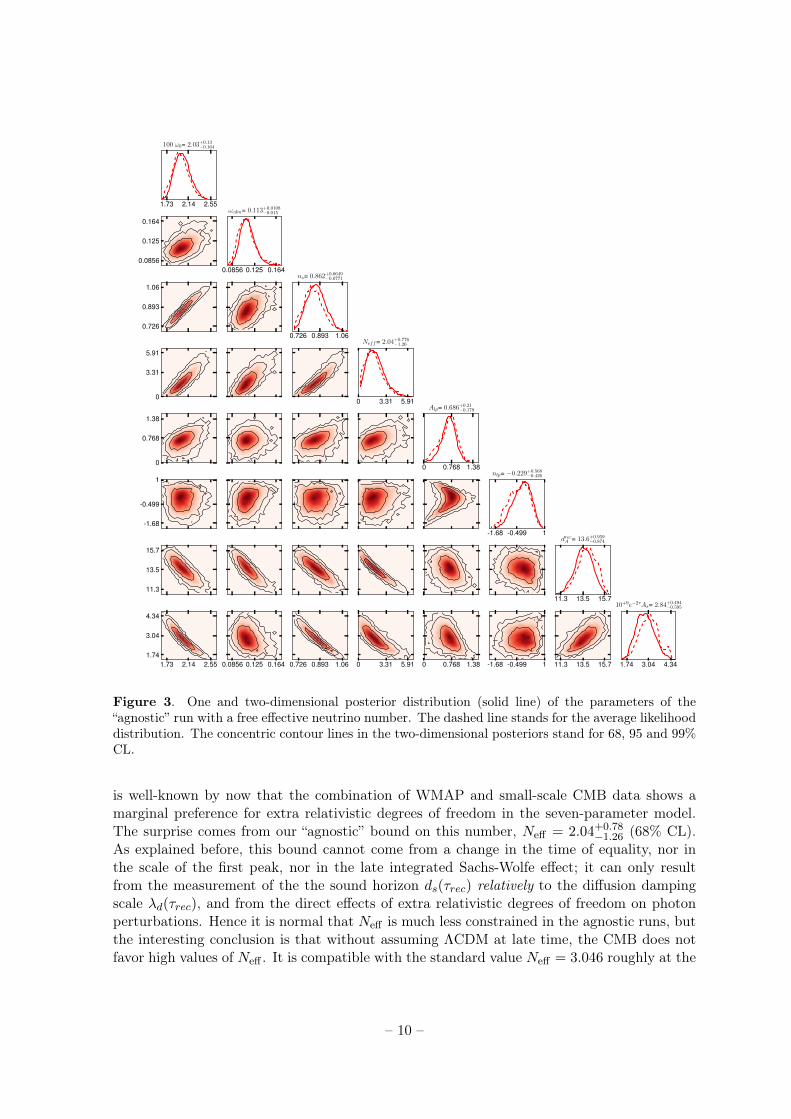
Figure 3. One and two-dimensional posterior distribution (solid line) of the parameters of the“agnostic” run with a free effective neutrino number. The dashed line stands for the average likelihooddistribution. The concentric contour lines in the two-dimensional posteriors stand for 68, 95 and 99%CL.

is well-known by now that the combination of WMAP and small-scale CMB data shows amarginal preference for extra relativistic degrees of freedom in the seven-parameter model.The surprise comes from our “agnostic” bound on this number, Neff = 2.04+0.78

−1.26 (68% CL).As explained before, this bound cannot come from a change in the time of equality, nor inthe scale of the first peak, nor in the late integrated Sachs-Wolfe effect; it can only resultfrom the measurement of the the sound horizon ds(τrec) relatively to the diffusion dampingscale λd(τrec), and from the direct effects of extra relativistic degrees of freedom on photonperturbations. Hence it is normal that Neff is much less constrained in the agnostic runs, butthe interesting conclusion is that without assuming ΛCDM at late time, the CMB does notfavor high values of Neff . It is compatible with the standard value Neff = 3.046 roughly at the

– 10 –

100 ωb ωcdm ns Mν (eV) dArec 109e−2τAs Alp nlp

ΛCDM

2.205+0.046−0.049 0.114+0.0052

−0.0050 0.949+0.014−0.013 < 1.4 12.86+0.13

−0.13 2.16+0.10−0.12

` ≥ 100, marginalization over lensing potential amplitude and tilt

2.136+0.065−0.072 0.123+0.009

−0.010 0.920+0.025−0.025 < 1.8 12.69+0.19

−0.19 2.43+0.21−0.28 0.81+0.22

−0.16 −0.11+0.58−0.32

Table 3. Limits at the 68% confidence level of the minimum credible interval of model parameters(excepted for Mν , for which we show the 95% CL upper limit). The ΛCDM+Mν model of the firstline has a seventh independent parameter (zreio) that we do not show. We do not show either thelimits on the three nuisance parameters associated to the SPT likelihood.

one-σ level, with even a marginal preference for smaller values. This shows that recent hintsfor extra relativistic relics in the universe disappear completely if we discard any informationon the late time cosmological evolution. It is well-known that Neff is very correlated with H0

and affected by the inclusion of late cosmology data sets, like direct measurement of H0 or ofthe BAO scale. Our new result shows that even at the level of CMB data only, the marginalhint for large Neff is driven by physical effects related to late cosmology (and in particular bythe angular diameter distance to last scattering as predicted in ΛCDM).

The triangle plot in Figure 3 shows that in the agnostic run, Neff is still very correlatedwith other parameters such as ωb, ωcdm and ns. Low values of Neff (significantly smaller thanthe standard value 3.046) are only compatible with a very small ωb, ωcdm and ns. Note thatin this work, we assume standard BBN in order to predict YHe as a function of ωb (and ofNeff when this parameter is also left free), but we do not incorporate data on light elementabundances. By doing so, we would favor the highest values of ωb in the range allowed bythe current analysis (ωb ∼ 0.022), and because of parameter correlations we would also favorthe highest values of ωcdm, ns and Neff , getting close to the best-fitting values in the minimalearly cosmology model with Neff ∼ 3.046.

For neutrino masses, we performed two similar runs (summarised in Table 3 and Fig-ure 4), with now Mν being the additional parameter (assuming three degenerate neutrinospecies). In the ΛCDM case, our result Mν < 1.4 eV (95%CL) is consistent with the restof the literature, and close to the WMAP-only bound of [5]: measuring the CMB dampingtail does not bring significant additional information on the neutrino mass. In the agnosticrun, this constraint only degrades to Mν < 1.8 eV (95%CL). This limit is consistent withthe idea that for sufficiently large mν , the CMB can set a limit on the neutrino mass notjust through its impact on the background evolution at late time (and its contribution toωm today), but also through direct effects occurring at the time of recombination and soonafter. It is remarkable that this is true even for neutrinos of individual mass mν ∼ 0.6 eV,becoming non-relativistic precisely at the time of photon decoupling. The conclusion that theCMB is not compatible with neutrinos becoming non-relativistic before zrec (and not evenslightly before!) appears to be very robust, and independent of any constraint on the latecosmological evolution.

– 11 –

1.96 2.15 2.35

100 ωb= 2.14+0.0647−0.072

0.1 0.129 0.157

ωcdm= 0.123+0.00883−0.00979

0.1

0.129

0.157

0.849 0.923 0.997

ns= 0.92+0.0254−0.0252

0.849

0.923

0.997

0.1 0.814 1.39

Alp= 0.811+0.218−0.159

0.1

0.814

1.39

-1.4 -0.339 1

nlp= −0.113+0.578−0.319

-1.4

-0.339

1

0 0.467 0.841

Mν/3= 0.278+0.0959−0.278

0

0.467

0.841

12.1 12.6 13.2

drecA = 12.7+0.194−0.185

12.1

12.6

13.2

1.84 2.57 3.31

10+9e−2τAs= 2.43+0.215−0.276

1.96 2.15 2.351.84

2.57

3.31

0.1 0.129 0.157 0.849 0.923 0.997 0.1 0.814 1.39 -1.4 -0.339 1 0 0.467 0.841 12.1 12.6 13.2

Figure 4. One and two-dimensional posterior distribution (solid line) of the parameters of the“agnostic” run with a total neutrino mass Mν (assuming three degenerate neutrinos of individualmass mν). Again, dashed line stands for average likelihood distribution, contour lines indicate the68, 95 and 99% CL.

5 Advantages of Monte Python

The results of this paper were obtained with the new parameter inference code MontePython, that we release publicly together with this article. Currently, Monte Python isinterfaced with the Boltzmann code class, and explores parameter space with the Metropolis-Hastings algorithm, just like CosmoMC3 (note however that interfacing it with other codesand switching to other exploration algorithms would be easy, thanks to the modular archi-tecture of the code). Hence, the difference with CosmoMC [4] does not reside in a radically

3In this paper we refer to the version of CosmoMC available at the time of submitting, i.e. the version ofOctober 2012.

– 12 –

different strategy, but in several details aiming at making the user’s life easy. It is not ourgoal to describe here all the features implemented in Monte Python: for that, we refer thereader to the documentation distributed with the code. We only present here a brief summaryof the main specificities of Monte Python.

Language and compilation. As suggested by its name, Monte Python is a MonteCarlo code written in Python. This high-level language allows to code with a very concisestyle: Monte Python is compact, and the implementation of e.g. new likelihoods requiresvery few lines. Python is also ideal for wrapping other codes from different languages: MontePython needs to call class, written in C, and the WMAP likelihood code, written in Fortran90. The user not familiar with Python should not worry: for most purposes, Monte Pythondoes not need to be edited, when CosmoMC would need to: this is explained in the fourthparagraph below.Another advantage of Python is that it includes many libraries (and an easy way to addmore), so that Monte Python is self-contained. Only the WMAP likelihood code needsits own external libraries, as usual. Python codes do not require a compilation step. Hence,provided that the user has Python 2.7 installed on his/her computer4 alongside very standardmodules, the code only needs to be downloaded, and is ready to work with.

Modularity. A parameter inference code is based on distinct blocks: a likelihood ex-ploration algorithm, an interface with a code computing theoretical predictions (in our case,a Boltzmann code solving the cosmological background and perturbation evolution), and aninterface with each experimental likelihood. In Monte Python, all three blocks are clearlysplit in distinct modules. This would make it easy, e.g., to interface Monte Python withcamb [12] instead of class, or to switch from the in-build Metropolis-Hastings algorithm toanother method, e.g. a nested sampling algorithm.The design choice of the code has been to write these modules as different classes, in the senseof C++, whenever it served a purpose. For instance, all likelihoods are defined as separatedclasses. It allows for easy and intuitive way of comparing two runs, and helps simplify thecode. The cosmological module is also defined as a class, with a defined amount of functions.If someone writes a python wrapper for camb defining these same functions, then MontePython would be ready to serve.On the other hand the likelihood exploration part is contained in a normal file, defining onlyfunctions. The actual computation is only done in the file code/mcmc.py, so it is easy toimplement a different exploration algorithm. From the rest of the code, this step would beas transparent as possible.In Python, like in C++, a class can inherit properties from a parent class. This becomesparticularly powerful when dealing with data likelihoods. Each likelihood will inherit froma basic likelihood class, able to read data files, and to treat storage. In order to imple-ment a new likelihood, one then only needs to write the computation part, leaving the restautomatically done by the main code. This avoids several repetitions of the same piece ofcode. Furthermore, if the likelihood falls in a generic category, like CMB likelihoods based onreading a file in the format .newdat (same files as in CosmoMC), it will inherit more preciseproperties from the likelihood_newdat class, which is itself a daughter of the likelihoodclass. Hence, in order to incorporate CMB likelihoods apart from WMAP, one only needs towrite one line of python for each new case: it is enough to tell, e.g., to the class accounting for

4The documentation explains how to run with Python 2.6. The code would require very minimal modifi-cations to run with Python 3.0.

– 13 –

the CMB experiment SPT that it inherits all properties from the generic likelihood_newdatclass. Then, this class is ready to read a file in the .newdat format and to work. Note thatour code already incorporates another generic likelihood class that will be useful in the futurefor reading Planck likelihoods, after the release of Planck data.Finally, please note that these few lines of code to write for a new likelihood are completelyoutside the main code containing the exploration algorithm, and the cosmological module.You do not need to tell the rest of the code that you wrote something new, you just have touse your new likelihood by its name in a starting parameter file.

Memory keeping and safe running. Each given run, i.e. each given combination ofa set of parameters to vary, a set of likelihoods to fit, and a version of the Boltzmann code,is associated to a given directory where the chains are written (e.g. it could be a directorycalled chains/wmap_spt/lcdm). All information about the run is logged automatically inthis directory, in a file log.param, at the time when the first chain is started. This filecontains the parameter names, ranges and priors, the list of extra parameters, the version ofthe Boltzmann code, the version and the characteristics of each data likelihood, etc. Hencethe user will always remember the details of a previous run.Moreover, when a new chain is started, the code reads this log file (taking full advantage ofthe class structure of the code). If the user started the new chain with an input file, thecode will compare all the data in the input file with the data in the log.param file. If theyare different, the code complains and stop. The user can then take two decisions: eithersome characteristic of the run has been changed without noticing, and the input file can becorrected. Or it has been changed on purpose, then this is a new run and the user mustrequire a different output directory. This avoids the classical mistake of mixing unwillinglysome chains that should not be compared to each other. Now, if the input file is similar tothe log.param file, the chain will start (it will not take the same name as previous chains:it will append automatically to its name a number equal to the first available number in thechain directory). In addition, the user who wishes to launch new chains for the same run canomit to pass an input file: in this case all the information about the run is automatically readin the log.param and the chain can start.The existence of log.param file has another advantage. When one wants to analyze chainsand produce result files and plots (the equivalent of running Getdist and matlab or maplein the case of CosmoMC), one simply needs to tell Monte Python to analyze a givendirectory. It is not needed to pass another input file, since all information on parameternames and ranges will be found in the log.param. If the output needs to be customized (i.e.,changing the name of the parameters, plotting only a few of them, rescaling them by somefactor, etc.), then the user can use command lines and eventually pass one small input filewith extra information.

No need to edit the code when adding parameters. The name of cosmologicalparameters is never defined in Monte Python. The code only knows that in the input file,it will read a list of parameter names (e.g. omega_b, z_reio, etc.) and pass this list to thecosmology code together with some values. The cosmology code (in our case, class) willread these names and values as if they were written in an input file. If one of the names isnot understood by the cosmology code, the run stops. The advantage is that the user canimmediately write in the input file any name understood by class, without needing to editMonte Python. This is not the case with CosmoMC. This is why users can do lots of thingswith Monte Python without ever needing to edit it or even knowing Python. If one wants

– 14 –

to explore a completely new cosmological model, it is enough to check that it is implementedin class (or to implement it oneself and recompile the class python wrapper). But MontePython doesn’t need to know about the change. To be precise, in the Monte Pythoninput file, the user is expected to pass the name, value, prior edge etc. of all parameters (i)to be varied; (ii) to be fixed; (iii) to be stored in the chains as derived parameters. Thesecan be any class parameter: cosmological parameters, precision parameters, flags, input filenames. Let us take two examples:

• In this paper, we showed some posterior probabilities for the angular diameter distanceup to recombination. It turns out that this parameter is always computed and storedby class, under the name ‘da_rec’. Hence we only needed to write in the input file ofMonte Python a line looking roughly like da_rec=‘derived’ (see the documentationfor the exact syntax), and this parameter was stored in the chains. In this case MontePython did not need editing.

• We used in this work the parameter [e−2τAs]. To implement this, there would be twopossibilities. The public class version understands the parameters τ and As. The firstpossibility is to modify the class input module, teach it to check if there is an inputparameter ‘exp_m_two_tau_A_s’, and if there is, to infer As from [e−2τAs] and τ . Thenthere is no need to edit Monte Python. However, in a case like this, it is actuallymuch simpler to leave class unchanged and to add two lines in the Monte Pythonfile data.py. There is a place in this file devoted to internal parameter redefinition. Theuser can add two simple lines to tell Monte Python to map (‘exp_m_two_tau_A_s’,‘tau’) to (‘A_s’, ‘tau’) before calling class. This is very basic and does not requireto know python. All these parameter manipulations are particularly quick and easywith Monte Python.

The user is also free to rescale a parameter (e.g. As to 109As in order to avoid dealing withexponents everywhere) by specifying a rescaling factor in the input file of Monte Python:so this can be done without editing neither Monte Python nor class.Please note however that, while this is true that any input parameter will be understooddirectly by the code, to recover derived parameters, the wrapper routine (distributed withclass) should know about them. To this end, we implemented what we think is a near-completelist of possible derived parameters in the latest version of the wrapper.

Playing with covariance matrices. When chains are analyzed, the covariance matrixis stored together with parameter names. When this matrix is passed as input at the beginningof the new run, these names are read. The code will then do automatically all the necessarymatrix manipulation steps needed to get all possible information from this matrix if the listof parameter has changed: this includes parameter reordering and rescaling, getting rid ofparameters in the matrix not used in the new runs, and adding to the matrix some diagonalelements corresponding to new parameters. All the steps are printed on screen for the userto make sure the proper matrix is used.

Friendly plotting. The chains produced by Monte Python are exactly in the sameformat as those produced by CosmoMC: the user is free to analyze them with GetDist orwith a customized code. However Monte Python incorporates its own analysis module,that produce output files and one or two dimensional plots in PDF format (including theusual "triangle plot"). Thanks to the existence of log.param files, we just need to tellMonte Python to analyze a given directory - no other input is needed. Information on

– 15 –

the parameter best-fit, mean, minimal credible intervals, convergence, etc., are then writtenin three output files with different presentation: a text file with horizontal ordering of theparameters, a text file with vertical ordering, and a latex file producing a latex table. In theplots, the code will convert parameter names to latex format automatically (at least in thesimplest case) in order to write nice labels (e.g. it has a routine that will automatically replacetau_reio by \tau_reio). If the output needs to be customized (i.e., changing the nameof the parameters, plotting only a few of them, rescaling them by some factor, etc.), then theuser can use command lines and eventually pass one small input file with extra information.The code stores in the directory of the run only a few PDF files (by default, only two; moreif the user asks for individual parameter plots), instead of lots of data files that would beneeded if we were relying on an external plotting software like Matlab.

Convenient use of mock data. The released version of Monte Python includessimplified likelihood codes mimicking the sensitivity of Planck, of a Euclid-like galaxy redshiftsurvey, and of a Euclid-like cosmic shear survey. The users can take inspiration from thesemodules to build other mock data likelihoods. They have been developed in such way thatdealing with mock data is easy and fully automatized. The first time that a run is launched,Monte Python will find that the mock data file does not exist, and will create one using thefiducial model parameters passed in input. In the next runs, the power spectra of the fiducialmodel will be used as an ordinary data set. This approach is similar to the one developed inthe code FuturCMB5 [13] compatible with CosmoMC, except that the same steps needed tobe performed manually.

6 Conclusions

Models for the latest stages of the cosmological evolution rely on a less solid theoretical andobservational ground than the description of earlier stages, like BBN and recombination.Reference [1] suggested a way to infer parameters from CMB data under some assumptionsabout early cosmology, but without priors on late cosmology. By standard assumption onearly cosmology, we understand essentially the standard model of recombination in a flatFriedmann-Lemaître universe, assuming Einstein gravity, and using a consistency relationbetween the baryon and Helium abundance inferred from standard BBN. The priors on latecosmology that we wish to avoid are models for the acceleration of the universe at smallredshift, a possible curvature dominated stage, possible deviations from Einstein gravity onvery large scale showing up only at late times, and reionization models.

We explained how to carry such an analysis very simply, pushing the method of [1] toa higher precision level by introducing a marginalization over the amplitude and tilt of theCMB lensing potential. We analyzed the most recent available WMAP and SPT data inthis fashion, that we called “agnostic” throughout the paper. Our agnostic bounds on theminimal “early cosmology” model are about twice weaker than in a standard ΛCDM analysis,but perfectly compatible with ΛCDM results: there is no evidence that the modeling of thelate-time evolution of the background evolution, thermal history and perturbation growth inthe ΛCDM is a bad model, otherwise it would tilt the constraints on ωb, ωcdm and ns awayfrom the “agnostic” results. It is interesting that WMAP and SPT alone favor a level of CMBlensing different from zero and compatible with ΛCDM predictions.

We extended the analysis to two non-minimal models changing the “early cosmology”,with either a free density of ultra-relativistic relics, or some massive neutrinos that could

5http://lpsc.in2p3.fr/perotto/

– 16 –

become non-relativistic before or around photon decoupling. In the case of free Neff , it isstriking that the “agnostic” analysis removes any hint in favor of extra relics. The allowedrange is compatible with the standard value Neff = 3.046 roughly at the one-sigma level, witha mean smaller than three. In the case with free total neutrino massMν , it is remarkable thatthe “agnostic” analysis remains sensitive to this mass: the two-sigma bound coincides almostexactly with the value of individual masses corresponding to a non-relativistic transitiontaking place at the time of photon decoupling.

The derivation of these robust bounds was also for us an occasion to describe the mainfeature of the new parameter inference code Monte Python, that we release together withthis paper. Monte Python is an alternative to CosmoMC, interfaced with the Boltzmanncode class. It relies on the same basic algorithm as CosmoMC, but offers a variety of user-friendly function, that make it suitable for a wide range of cosmological parameter inferenceanalyses.

Acknowledgments

We would like to thank Martin Kilbinger for useful discussions. We are also very muchindebted to Wessel Valkenburg for coming up with the most appropriate name possible forthe code. This project is supported by a research grant from the Swiss National ScienceFoundation.

References

[1] M. Vonlanthen, S. Rasanen and R. Durrer, JCAP 1008 (2010) 023 [arXiv:1003.0810[astro-ph.CO]].

[2] J. Lesgourgues, arXiv:1104.2932 [astro-ph.IM].

[3] D. Blas, J. Lesgourgues and T. Tram, JCAP 1107 (2011) 034 [arXiv:1104.2933 [astro-ph.CO]].

[4] A. Lewis and S. Bridle, Phys. Rev. D 66 (2002) 103511 [astro-ph/0205436].

[5] E. Komatsu et al. [WMAP Collaboration], Astrophys. J. Suppl. 192 (2011) 18[arXiv:1001.4538 [astro-ph.CO]].

[6] C. L. Reichardt, L. Shaw, O. Zahn, K. A. Aird, B. A. Benson, L. E. Bleem, J. E. Carlstromand C. L. Chang et al., Astrophys. J. 755 (2012) 70 [arXiv:1111.0932 [astro-ph.CO]].

[7] J. Hamann, J. Lesgourgues and G. Mangano, JCAP 0803 (2008) 004 [arXiv:0712.2826[astro-ph]].

[8] G. Mangano, G. Miele, S. Pastor and M. Peloso, Phys. Lett. B 534 (2002) 8 [astro-ph/0111408].

[9] W. Hu and N. Sugiyama, Astrophys. J. 471 (1996) 542 [astro-ph/9510117].

[10] S. Bashinsky and U. Seljak, Phys. Rev. D 69 (2004) 083002 [astro-ph/0310198].

[11] R. Keisler, C. L. Reichardt, K. A. Aird, B. A. Benson, L. E. Bleem, J. E. Carlstrom,C. L. Chang and H. M. Cho et al., Astrophys. J. 743 (2011) 28 [arXiv:1105.3182 [astro-ph.CO]].

[12] A. Lewis, A. Challinor and A. Lasenby, Astrophys. J. 538 (2000) 473 [astro-ph/9911177].

[13] L. Perotto, J. Lesgourgues, S. Hannestad, H. Tu and Y. Y. Y. Wong, JCAP 0610 (2006) 013[astro-ph/0606227].

– 17 –