Consequences of Mandated Bank Liquidity Disclosures

Anya Kleymenova*

London Business School

Regent’s Park

London NW1 4SA, UK

akleymenova@london.edu

November 2013

PRELIMINARY

Please do not quote or circulate without permission.

Abstract

This paper studies the capital market consequences of unique and unexpected mandatory disclosures

of banks’ liquidity and the resulting changes in banks’ behavior. I employ a hand-collected sample of

the disclosures of banks’ borrowing from the US Federal Reserve Discount Window (DW) during the

financial crisis. I find that these disclosures contain positive incremental market information as they

decrease banks’ cost of capital (measured by the equity bid-ask spreads and the cost of debt).

However, I also find evidence of endogenous costs associated with more disclosure. I document that

banks respond to the DW disclosures by increasing their liquidity holdings and decreasing risky

assets. In line with the theoretical predictions of Goldstein and Sapra (2013), this finding indicates

that, following the DW disclosures, banks try to avoid accessing the DW facility, despite its cost of

capital benefits.

JEL classification: G18, G21, G28, M41

Keywords: Liquidity disclosure, discount window, consequences of disclosure, bank liquidity,

prudential regulation of banks.

* I started work on this paper during my PhD research internship at the Bank of England. I would like to thank

the chair of my dissertation committee, Florin Vasvari, as well as Rhiannon Sowerbutts from the Bank of

England for their generous support and guidance throughout this project. Discussions with Pat Akey, Allen

Berger, Christa Bouwman, Michael Crawley (discussant), Emmanuel De George, Atif Ellahie, Sapnoti Eswar,

John Kuong, Elizabeth Klee, Yun Lou, Maria Loumioti, Clemens Otto, Richard Rosen (discussant), Oded

Rozenbaum, Oleg Rubanov, Tjomme Rusticus, Stephen Schaefer, Sasan Saiy (discussant), Haresh Sapra, İrem

Tuna, Oktay Urcan, Joana Valente, Robert Verrecchia, and Irina Zviadadze have been extremely helpful. I

would also like to thank the participants of two internal Financial Stability Prudential Policy Division seminars

at the Bank of England, the 2013 Trans-Atlantic Doctoral Conference, the 2013 ABTA Doctoral Researcher

Awards, the 2013 FIRS Conference, the 2013 IFABS Conference, the 2013 AAA Annual Meeting, and the

London Business School for their helpful comments and suggestions. I gratefully acknowledge the financial

support of the Economic & Social Research Council and the London Business School. The views expressed in

this paper are my own and are not necessarily the views of the Bank of England. All remaining errors are my

own.

1

1. Introduction

The health of a financial sector relies crucially on its liquidity, as evidenced by the recent

events that triggered the financial crisis. Several regulatory proposals have been put forward

with the aim of preventing a recurrence of these events, a number of which involve the

disclosure of bank liquidity information. The reasoning is that greater transparency would

allow market participants and bank counterparties to discipline banks (BIS 2013a, 2013b).

Opponents of these proposals, however, argue that, in the presence of information asymmetry

about banks’ asset quality and a lack of credible communication, liquidity disclosures can be

counterproductive because they might lead to decreased lending and avoidance of borrowing

from the lender of last resort (Herzberg and Praet, 2008; Bernanke, 2009; and Thakor, 2012).

This paper studies the capital market consequences of bank liquidity disclosures and the

impact of these disclosures on banks’ behavior.

I utilize information from the 2011 US Federal Reserve disclosures that reveal which

banks accessed the Discount Window (DW) liquidity facilities.1 During the 2007-2009

financial crisis, banks in the United States borrowed unprecedented amounts through the DW

facilities. While weekly borrowing from the DW before the crisis averaged $170 million per

week, this amount was close to $30.8 billion from August 2007 to December 2009. Banks

borrowed more than 26,000 loans with a total par value of $11 trillion. More than 50% (20%)

of large (small) banks used the DW between March 2008 and March 2010 to obtain

additional liquidity (Berger et al., 2013). However, despite the sizeable amount of capital

provided, information about individual bank borrowing from the DW was not made public

1 The DW, established in 1913, is a facility that allows deposit-taking institutions in the United States to borrow

funds from the US Federal Reserve System on an overnight basis when needed (also known as the “lender of

last resort”). The DW extends credit to help alleviate liquidity strains in deposit institutions and ensure the basic

stability of the payment system. Banks pre-pledge collateral and can access this facility on a “no-questions-

asked” basis, provided they have sufficient collateral and remain sound. During the financial crisis, the US

Federal Reserve increased the maturity of DW loans to the maximum maturity of 90 days.

2

until recently. On March 21, 2011, the Supreme Court ruled in favor of several US news

networks and, on March 31, 2011, forced the Federal Reserve to reveal which banks accessed

the DW facilities, when they did so, how much they borrowed and for how long.2 This

disclosure was an “information surprise” that can provide insight into how banks modify their

behavior if liquidity disclosures are provided regularly. Using a propensity-score matched

sample of banks that accessed the DW (treatment sample) and those that did not (control

sample), along with a standard difference-in-differences methodology, I study two main

research questions: (1) whether the DW disclosures had any consequences with respect to

banks’ cost of capital; and (2) whether these disclosures triggered changes in banks’

borrowing and lending activities.

Previous research has documented the existence of a stigma associated with the usage

of the DW by banks in the United States (Furfine, 2001 and 2003; Armantier et al., 2011; and

Acharya, Gromb and Yorulmazer, 2012). Ennis and Weinberg (2013) show analytically that

in the presence of information asymmetry about the quality of banks’ assets, it is rational for

banks to avoid using the DW facilities to prevent signaling that their need for funding might

be an indicator of poor asset quality. While the DW borrowing rate should theoretically

provide an upper-bound on banks’ cost of short-term borrowing in the federal funds market

(Acharya et al., 2012), in fact, banks are willing to pay higher rates on funds from other

sources, such as interbank loans or the Term Auction Facility, TAF (Furfine, 2003).3

Furthermore, despite the fact that funds provided through the DW and TAF had the same

collateral and eligibility requirements, banks borrowed substantially higher amounts during

2 Bloomberg News and Fox News filed several lawsuits against the Federal Reserve under the Freedom of

Information Act requesting access to the DW borrowing data during the financial crisis (please see Appendix A

for the timeline of the lawsuits). For the news coverage, see, for example, Torres, Craig (2011), “Fed Releases

Discount-Window Loan Records During Crisis Under Court Order,” Bloomberg, March 31, 2011, available at

http://www.bloomberg.com/news/2011-03-31/federal-reserve-releases-discount-window-loan-records-under-

court-order.html. 3 The Term Auction Facility (TAF) was a temporary facility in operation from December 2007 until March

2010.

3

the financial crisis through the more expensive TAF and thus paid substantially more because

of the perceived DW stigma (Brunnermeier, 2009; and Haltom, 2011).4

While the

aforementioned studies all document the existence of the DW stigma by comparing banks’

borrowing in the federal funds (or interbank) market to that of borrowing from the Federal

Reserve, the unprecedented event of the full, public DW borrowing disclosure provides a

unique opportunity to test whether the stigma exists in the public capital market as well. If the

market penalizes banks when the information is revealed, then it is rational for banks to

adjust their behavior pre-emptively to avoid the impact of future DW disclosures.

Prior analytical research on disclosure has mainly focused on studying the effects of

mandatory and voluntary disclosures by management and the role disclosure plays in

informing capital market investors about a firm’s future profitability (e.g., Kim and

Verrecchia, 1994; and Lambert, Leuz and Verrecchia, 2012). These studies find that

disclosure improves price efficiency by decreasing information asymmetry. Less is known,

however, about the cost of capital impact of specific firm disclosures provided by regulators.

The notable exceptions are the recent studies of the capital market consequences of US and

EU bank stress test disclosures on the information asymmetry and information uncertainty

about the underlying soundness of financial institutions (Peristiani, Morgan and Savino,

2010; Bischof and Daske, 2013; and Ellahie, 2013). Regulators potentially have a different

objective function than an individual firm. In particular, banking regulators aim to provide

disclosures that enhance market discipline and, at the same time, improve financial stability

of the banking sector (Morgan and Stiroh, 2001; Goldstein and Sapra, 2013). Furthermore,

regulatory disclosures might be viewed by market participants as less strategic for an

individual firm than an individual firm’s disclosure, thus potentially increasing the credibility

4 In particular, during the 28 months of TAF’s operation, financial institutions borrowed more than $3.8 trillion

of funds at an average premium of between 37 and 150 basis points above the DW rate (Haltom, 2011).

4

of disclosures. Finally, disclosures by regulators might provide further impetus for additional

voluntary disclosures by firms wishing to signal their quality (Bischof and Daske, 2013).

While more disclosure improves price efficiency and leads to market discipline in a

setting without frictions, Goldstein and Sapra (2013) demonstrate analytically that this might

not necessary be the case for banks. This is because banks operate in the “second-best”

environment, due to their interconnected nature, the presence of externalities, and banks’

exposure to informational and market frictions. Furthermore, they show that, in the second-

best environment, the incentives of all market participants need to be taken into account—for

example, the incentives of banks when they interact with each other in the interbank market.

Therefore, Goldstein and Sapra (2013) argue that while more disclosure for banks might lead

to better market discipline and price efficiency, it is a necessary but insufficient condition for

economic efficiency because of the endogenous costs of disclosure. Similarly, Thakor (2012)

analytically predicts that mandatory financial disclosure for financial institutions might be

inefficient and lead to banks’ fragility. Overall, these two studies argue that, in response to

increased mandatory disclosure, banks change their behavior to avoid further disclosures.

To study the first question about the effect of liquidity disclosure on banks’ cost of

capital, I first need to establish that the information released by the Federal Reserve was

material. I assess the information content of DW disclosures using three measures:

cumulative abnormal stock returns (Lo, 2003; and Larcker, Ormazabal and Taylor, 2011);

abnormal stock return volatility (Landsman and Maydew, 2002); and abnormal trading

volume (Beaver, 1968; and Kim and Verrecchia, 1997). I find that, following the disclosure

of the DW information, banks that accessed the DW exhibit positive cumulative abnormal

returns of 1.10% (measured over a four-day window, including the DW disclosure event)

compared to banks that did not. I also find that banks that accessed the DW experience a 26%

drop in abnormal trading volume. However, I do not find any significant abnormal return

5

volatility following the DW event, suggesting that negative abnormal volumes are more

likely to be the result of investors’ consensus, as investors will trade less if there is no

disagreement about the content of disclosure (Holthausen and Verrecchia, 1990). These

initial information content tests suggest that investors see the DW disclosures as a positive

material event. Furthermore, the significant results indicate that the DW disclosures provide

incremental material information despite being released with a two-year lag.

Next, I directly investigate the cost of capital consequences of DW disclosures by

studying changes in the equity bid-ask spread and the cost of debt. I find that the DW

disclosures significantly decrease the information asymmetry component of the bid-ask

spreads for banks that accessed the DW in the short-horizon of seven days around the

announcement date. However, I find that the information asymmetry component of the bid-

ask spread increases for banks that accessed the DW over the longer horizon of two quarters

after the event. Regarding the cost of debt, I find that following the DW disclosures, banks

that accessed the DW receive significantly lower bond issuing yields, with an average

significant reduction of 1.16 percentage points, compared to the matched control group of

banks that did not access the DW facilities. Overall, these findings suggest that the DW

disclosures result in a decrease in the banks’ cost of capital as measured by short-term equity

and debt prices. Furthermore, unlike in prior studies, which document the existence of the

DW stigma in the interbank market, there seems to be no evidence suggesting the stigma’s

presence in the public capital markets.

Finally, I study the effects of the DW disclosures on banks’ lending, liquidity, and

borrowing to establish whether banks change their behavior in response to the DW

disclosures. I document that, following the DW disclosures, banks increase liquidity and

decrease asset risk, measured as a proportion of risk-weighted assets in total assets. Banks

also decrease their borrowing from other sources of unsecured lending, given by the

6

proportion of their pledged assets in total assets. Furthermore, banks that accessed the DW

appear to borrow less from the interbank market and increase their balance sheet liquidity by

closing the loan-to-deposit gap. In addition, banks that borrowed more or accessed the DW

more frequently decrease their risky lending and increase liquidity. Therefore, banks appear

to change the composition of their balance sheets and hold more liquidity following the DW

disclosures. These results, taken together with the capital market tests, suggest that while the

DW disclosures provide some incremental information and are perceived positively by equity

and debt investors, they also create incentives for banks to avoid accessing the DW in the

future, despite the capital market benefits. This seeming inefficiency is an example of the

endogenous costs (or unintended consequences) of disclosure discussed by Goldstein and

Sapra (2013) and Gigler et al. (2013). In this setting, the endogenous cost of disclosure for

banks is the potential increase in the cost of interbank borrowing due to the signal that DW

disclosures provide about banks’ liquidity needs and the quality of their assets.

This study contributes to the literature across several dimensions. First, it adds to the

literature on the role and economic consequences of mandatory disclosure. There is ample

literature on the capital market consequences of mandated changes of particular accounting

standards, rules, or regulatory events.5 These studies reveal that mandatory disclosure leads to

a reduction in information asymmetry and firms’ cost of capital. I add to this literature by

documenting how unexpected mandatory liquidity disclosures by a regulator, at the time of

disclosure, provide incremental information to the capital market and lead to changes in

banks’ cost of capital. Mandatory disclosure by a regulator is an interesting setting as it

provides standardized information for all companies and is less likely to be influenced by the

strategic behavior of a particular firm. The unexpected nature of this disclosure allows me to

5 For example, see Watts and Zimmerman (1986); Fields, Lys and Vincent (2001); Kothari (2001); Leuz and

Verrecchia (2000); Daske et al., (2008, 2013); Hail, Leuz and Wysoki (2010); DeFond et al., (2011); Zhang,

(2007); and Petacchi (2012).

7

exploit the exogenous variation resulting from the information shock and hence to draw

causal inferences. Furthermore, I also contribute to the studies which investigate mandatory

disclosure by bank regulators during the recent financial crisis (e.g., Perestiani et al., 2010;

Bischof and Daske, 2013; and Ellahie, 2013). I add to these studies by providing evidence

that supplemental mandatory liquidity disclosures decrease cost of capital and lead to a

decrease in banks’ risk-taking behavior. Moreover, while these studies focus on the effect of

disclosure during the financial crisis, I show corroborating evidence that DW disclosures

provide incremental information to the capital markets even after the financial crisis.

Second, this paper contributes to the literature on the role of disclosure as a

disciplining device for financial institutions (Flannery, 1998; Flannery, Kwan and

Nimalendran, 2010; and Bushman and Williams, 2012). One of the arguments in support of

the DW disclosure is that it can improve market discipline by providing additional

information about banks’ asset quality and liquidity. As Beatty and Liao (2013) point out, it

is important to study and understand the effects of new regulatory changes for banks and, in

particular, the increased liquidity disclosure requirements. However, given that the regulation

affects all banks, studying the impact of these changes empirically poses a challenge of

constructing a counterfactual scenario. The setting of the unexpected liquidity disclosure

enables me to construct a counterfactual scenario of the consequences of liquidity disclosure

by comparing banks that were directly affected by these disclosures (banks accessing the

DW) with those that were not. My findings show that liquidity disclosures provide

incremental information to the capital market over and above that available in regulatory and

financial filings and result in the reduction in banks’ cost of capital.

Third, because banks operate in the second-best environment with informational and

market frictions, my setting allows me to directly test the endogenous costs of disclosure. In

line with the analytical predictions of Goldstein and Sapra (2013) and Thakor (2012), and in

8

contrast to the work that shows more disclosure is always better (e.g., Blackwell, 1951), I

find that banks change their behavior following the DW disclosures by decreasing asset risk

and increasing liquidity holdings. This is consistent with banks’ attempts to mitigate the

effects of similar disclosures in the future. Furthermore, banks change their behavior despite

the positive reaction in the public capital market, suggesting that they perceive these

disclosures to increase their cost of funding in some other way, in particular, through the

interbank market. This is an example of price efficiency not directly translating into

economic efficiency, as banks respond to disclosures by changing their ex ante behavior

(Bond, Edmans and Goldstein, 2012; Goldstein and Sapra, 2013; and Gigler et al., 2013).

Finally, this paper provides new evidence on whether the DW stigma is reflected in

the capital markets. Unlike the interbank markets, in which the existence of the stigma has

been widely documented (Furfine 2001; 2003; Armantier et al., 2011; and Acharya et al.,

2012), I find no supporting evidence for the existence of the DW stigma in the public capital

markets (either debt or equity). My findings also corroborate those of Berger et al. (2013),

who study which banks accessed the DW and TAF during the financial crisis and document

changes in banks’ lending behavior and balance sheet structure contemporaneously to their

usage of TAF and DW. My study differs in that it focuses on the capital market consequences

of the public disclosure of DW information and changes in banks’ behavior following this

disclosure. To the best of my knowledge, consequences of disclosing the DW information

have not yet been documented.

The rest of this paper is organized as follows: section 2 provides a brief history of the

discount window and its role; section 3 reviews the literature and formulates the hypotheses;

section 4 introduces data sources and discusses the research design; section 5 presents the

empirical results; and section 6 summarizes the main findings.

9

2. Borrowing from the Federal Reserve

The Discount Window (DW) facility at the Federal Reserve functions as a safety valve for

financial institutions. Through this facility, the Federal Reserve can act as a “lender of last

resort” and provide access to liquidity for solvent banks with sufficient collateral.6 Since

2003, depository institutions have been allowed to borrow from the DW easily and without

any questions asked.

While the function of the DW remained relatively constant, its administration has

changed over time. Prior to the mid-1960s, the DW loans were extended at “penalty” rates

equal to or higher than short-term market interest rates (Madigan and Nelson, 2002; and Klee,

2011). From the mid-1960s until January 2003, the rate paid on the discount window

borrowing was pegged at 25 to 50 basis points below the target federal funds rate and, to

reduce potential arbitrage opportunities, deposit institutions borrowing from the DW had to

demonstrate that they were unable to obtain funding from any other sources and were subject

to additional regulatory scrutiny. Accessing the DW, therefore, became associated with the

inability to borrow funds from other sources, giving rise to a stigma (Brunnermeier, 2009;

and Haltom, 2011). This regime changed in January 2003, when the Federal Reserve returned

to the “penalty rate” framework and increased the discount rate to 100 to 150 basis points

above the federal funds target rate. Two facilities were established: primary credit for

institutions in sound condition and secondary credit for financial institutions that do not

qualify for primary access funding. Primary access facility provides credit mainly overnight

on a “no-questions-asked” basis with minimal administration and no restrictions on its use.

Secondary credit is available to troubled financial institutions to meet overnight backup

6 All commercial banks, thrift institutions, and US branches and agencies of foreign banks have access to the

DW. The range of acceptable collateral includes investment-grade certificates of deposit, AAA-rated

commercial mortgage-backed securities, US Treasury securities, state and local government securities,

collateralized mortgage obligations (AAA), consumer loans, commercial and agricultural loans, and certain

mortgage notes on one-to-four family residences.

10

liquidity needs and is closely monitored by the Federal Reserve. These changes were

implemented as an attempt to eliminate the stigma associated with the DW access; however,

they were unsuccessful (Furfine, 2003; and Haltom, 2011). In this paper, I study banks that

access the primary credit facility of the DW.

As the financial crises unfolded in the second half of 2007, borrowing from the DW

remained low (Bernanke, 2009). In August 2007, the Federal Reserve reduced the spread

between the discount rate and the federal funds rate to 50 basis points and increased the DW

loan terms from overnight to 30 days. The Federal Reserve also introduced the Term Auction

Facility (TAF) to overcome the stigma problem associated with the DW (Bernanke, 2009).

The key difference between the DW and TAF was that TAF was administered through a

series of fortnightly auctions: the Federal Reserve announced that it would auction a fixed

amount of funds, and an unlimited number of banks could bid for up to 10% of that amount

(the cap was imposed to ensure that funds were distributed evenly). Funds were given to

bidders providing the highest bid, which exhausted all available funds. Furthermore, bidders

were only notified that their bid was successful three days after the auction had taken place.

Hence, TAF guaranteed that multiple banks were able to borrow from the Federal Reserve

and reduced the likelihood that any one borrower would be identified by the market as

requiring immediate funding and hence penalized (Armantier et al., 2011; and Haltom, 2011).

On March 31, 2011, the Federal Reserve made an unprecedented release of the DW

borrowing information after it had lost a series of lawsuits filed under the Freedom of

Information Act. The Federal Reserve initially refused to reveal this information by arguing

that such disclosure would dissuade banks from borrowing from the DW in the future and

thus undermine financial stability; however, just a few days earlier, on March 21, 2011, the

Supreme Court denied the Federal Reserve’s petition to hear its appeal. This was the first

11

time the DW information was made public since its inception in 1913.7 In addition, as

required by the Dodd-Frank Act, on December 1, 2010, the Federal Reserve released

information about TAF borrowing.

In this paper, I focus on the DW disclosures event on March 31, 2011 (the DW

disclosure event). In addition, in robustness tests, I also investigate the reaction to the TAF

disclosure event (December 1, 2010) and the Supreme Court decision event

(March 21, 2011).

3. Review of the literature and hypotheses development

As discussed briefly above, accessing the DW facility is associated with a stigma based on

the notion that only a bank in financial trouble will borrow funds from the Federal Reserve

over other sources of funds (e.g., Peristiani, 1998; and Armantier et al., 2011). Ennis and

Weinberg (2013) provide a formal model showing the existence and rationality of the stigma

as a result of information asymmetry and noisy signaling; while Furfine (2001; 2003) finds

empirical evidence in support of the stigma. In addition, studies of banks’ behavior during the

recent financial crisis reveal further support that, even during times when liquidity needs are

extreme, banks pay a substantial premium for other sources of funds instead of accessing the

DW (Armantier et al., 2011; and Acharya et al., 2012). One factor that contributed to the

existence of this stigma is information asymmetry about the quality of banks’ assets (Artuc

and Demiralp, 2010; and Furfine, 2001).

Information asymmetries create costs by introducing adverse selection into

transactions between buyers and sellers of firm shares, which is typically manifest in reduced

levels of liquidity for firm shares (e.g., Copeland and Galai, 1983; Kyle, 1985; and Glosten

and Milgrom, 1985). In order to overcome the reluctance of potential investors to hold firm

7 The Dodd-Frank Act introduced a requirement for the Federal Reserve to release the DW access details with a

two-year lag. The first release was on September 28, 2012. Going forward, this information will be released

quarterly.

12

shares in illiquid markets, firms issue capital at a discount. Discounting results in fewer

proceeds to the firm and hence higher cost of capital. The disclosure theory for capital

markets predicts that if informative disclosures are backed by commitment to increased levels

of disclosure, the information asymmetry component of the equity bid-ask spread should

decrease (Baiman and Verrecchia, 1996; Diamond and Verrecchia, 1991; and Verrecchia,

2001). However, if disclosure is partial, such as in the case of redacted disclosures, the equity

bid-ask spread will increase (Verrecchia and Weber, 2006). If, on the one hand, the stigma

associated with the DW also applies to the capital markets, the revelation of which banks

accessed the DW during the financial crisis will lead to a negative market reaction. On the

other hand, because banks accessing the DW are required to be in good standing and have

enough high quality collateral, the reaction might be positive. Over a short horizon, the

changes of investors’ beliefs based on changes in information asymmetry will result in

changes in the bid-ask spread and thus changes in the cost of equity capital.

One of the main arguments in support of the DW disclosure is that it provides

additional information about banks’ liquidity and asset quality and may increase market

discipline. Bank supervisors are willing to disclose information about banks to share the role

of policing bank risk with private investors, in particular, bondholders. Morgan and Stiroh

(2001) find that banks’ bondholders take into account the underlying risk of banks’ portfolios

of assets. However, the authors also find that investors appear to fail to incorporate all

information or fully penalize large or more opaque banks, suggesting that the disciplinary

mechanism partially fails for banks either considered to be “too big to fail” or “too difficult to

understand” by the bond market. Prior studies on the role of disclosure in the credit markets

have documented that while higher disclosure quality leads to a lower cost of debt (Sengupta,

1998; Yu, 2005), bond prices have high sensitivity to negative news (Easton, Monahan and

Vasvari, 2009). Therefore, if the DW disclosure increases transparency and hence reduces the

13

adverse selection costs for bondholders, the DW disclosures will be viewed as positive news

by bondholders as they will reduce the uncertainty associated with the quality of banks’

assets (Duffie and Lando, 2001). However, if banks accessing the DW are instead perceived

as having poor asset quality in line with the documented stigma, the reaction will be negative.

Given that the DW disclosures are provided with a lag, I expect to find no significant effect

on banks’ cost of capital if the DW disclosures do not contain any new information for banks’

investors.

The effects of the DW disclosures on cost of debt and equity are, therefore, unclear a

priori and the net impact of the two opposing effects has to be assessed empirically. In my

first hypothesis, I test whether the DW disclosures result in a change in the cost of banks’

capital as measured by the information asymmetry component of the equity bid-ask spread

and the offering bond yields:

H1: DW disclosures decrease (increase) banks’ cost of capital as measured by the

equity bid-ask spread and offering bond yields if they decrease information

asymmetry (increase DW stigma).

The literature on real effects of accounting disclosure emphasizes the two-way impact

between firm decisions and capital market pricing (e.g., Kanodia and Lee, 1998; Sapra, 2002;

and Kanodia, Sapra and Venugopalan, 2004). If the DW disclosures provide additional

information to banks’ investors, they will result in changes in banks’ cost of capital. Whether

banks adjust their behavior accordingly, however, is unclear. Banks operate in the second-

best environment with informational and market frictions and are prone to externalities.

Therefore, increased disclosure, even if it results in price efficiency, might not necessarily

lead to economic efficiency due to endogenous costs (Bond et al., 2012; Goldstein and Sapra,

2013; and Gigler et al., 2013). Furthermore, in the second-best environment, it is important to

take into account the effect of disclosure not only on market discipline but also on all market

14

participants, for example, the effect of disclosure on bank’s interactions with each other in the

interbank market (Goldstein and Sapra, 2013).

Goldstein and Sapra (2013) present a theoretical model in which a banking regulator

discloses the results of banks’ stress tests. They show that market discipline is a necessary but

insufficient condition for economic efficiency. This is because disclosure might induce

suboptimal ex post market externalities that would lead to excessive and inefficient reaction

to public news. This disclosure might also reduce traders’ incentives to gather information

and hence impose market discipline. Most importantly, this disclosure might lead banks to

change their behavior ex ante in anticipation of future disclosures and thus make ex post

inefficient decisions. The authors refer to these predicted outcomes as endogenous costs of

disclosure. In addition, Thakor’s (2012) theory of information disclosure with disagreement

examines the implications of mandatory disclosure for financial and non-financial firms. He

finds that banks optimally disclose less strategic information than non-financial firms and that

mandatory disclosure may make banks more fragile. However, in a recent empirical study of

the European banks’ response to the regulator’s disclosure of the EU banks’ stress tests

results, Bischof and Daske (2013) find that this mandatory disclosure causes banks to lower

their risk-taking behavior.

When the information about the DW access is released, the market is already aware of

the Dodd-Frank Act requirements to provide DW access disclosures from September 2012,

and that these DW disclosures apply to all banks accessing the DW.8 The unexpected

disclosure provides banks with a signal about how such disclosures will be viewed by banks’

investors over and above that of the overall passage of the Dodd-Frank Act, to which

investors had a mixed reaction (Gao, Liao and Wang, 2013). Hence, if banks perceive

8 While many of the Dodd-Frank provisions specifically target the largest financial institutions with total assets

in excess of $50 billion, the DW disclosure requirements affect all banks accessing the DW.

15

investors and counterparties to react negatively to the release of the DW information, they

would adjust their behavior before the scheduled information is released. Such real changes

in banks’ behavior are likely to decrease their likelihood of accessing the DW in the future. In

particular, if banks perceive that future DW disclosures will increase their cost of funding and

ability to access the interbank market, they will seek to obtain short-term liquidity from other

sources to avoid the impact of future disclosures. Furthermore, banks might change the

riskiness of their assets to avoid short-term liquidity needs that might require them accessing

the DW. Therefore, my second hypothesis tests whether banks alter the composition of their

balance sheets in response to this release of the DW borrowing information:

H2: Disclosure of the DW information ex post affects banks’ asset allocation,

liquidity, and risk decisions ex ante.

4. Data and empirical research design

4.1 Data and sample selection

The DW borrowing data for most of the financial crisis (March 2008 to March 2010) is

obtained directly from Bloomberg in the form of PDF files it received from the Federal

Reserve on March 31, 2011. DW data contains the name of the bank, the district Federal

Reserve from which the funds were borrowed, the amount borrowed, and the loan terms

(collateral and other identifying information is redacted). TAF data is obtained directly from

the Federal Reserve, following the mandatory release under the Dodd-Frank Act on

December 1, 2010. TAF data is available for the duration of the facility (December 2007 to

March 2010) and, apart from the actual information on loans, also includes data on

unencumbered collateral and its quality.

For accounting and regulatory data, I use the consolidated financial statements for

bank holding companies (FR Y-9C reports), which are publicly available on the Federal

16

Reserve Bank of Chicago website.9 Since internal financing from the parent company is the

cheapest form of funding, financial institutions are unlikely to access the DW unless they are

unable to obtain funds from the parent company (Kashyap, Rajan and Stein, 2002; Gatev and

Strahan, 2006; Ashcraft, 2008). Therefore, in my analysis, I focus on the top-level banks by

manually matching the codes of banks accessing the DW to their top-level bank or bank

holding company. The data is also complemented with the structural information from the

FDIC Call Reports for commercial banks to identify the top-level BHC as well as a manual

name match of the information revealed through the FDIC’s National Information Center.

Form FR Y-9C contains detailed information on the financial performance of BHCs, their

consolidated financial statements, and accompanying details as well as exposures and

regulatory capital details. This data is also supplemented with market data from CRSP, bond

issuance data from Mergent Fixed Income Securities Database (FISD), and accounting data

from Compustat.10

I also conduct an extensive news search using Factiva to ensure that no other market-

sensitive events occurred contemporaneously with the DW disclosures. Appendix C shows

the news coverage for the US banking sector during the DW disclosure as well as on placebo

dates the year before and after. As can be seen from the chart, DW news represented

approximately one-half of all news articles on the US financial sector on March 31, 2011.

DW did not feature at all in the news, either in the previous year or the year after.

I focus my study on public BHCs in order to establish the capital market response to

the DW disclosures. My final dataset consists of 197 banks that accessed the DW and 76

banks that accessed TAF. In particular, 138 of these banks accessed the DW only and 17

9 Data is available at http://www.chicagofed.org/webpages/banking/financial_institution_reports/bhc_data.cfm.

BHCs are required to submit their regulatory filings within two months after the end of each calendar quarter. 10

BHCs are manually matched to the identifying information on issuers based on CUSIP, location and name of

the top-level BHC and issuer identifying information in Mergent FISD.

17

banks accessed TAF only. 59 banks accessed both facilities.11

The sample also includes

banks that did not access either DW or TAF matched on their likelihood of accessing the DW

facilities using propensity-score matching. These banks form the control sample in my

analysis.

Table 1, Panel A presents the descriptive statistics for the main sample. Panel B

presents variables used in the cost of equity tests, and Panel C shows the summary statistics

for the variables used in the cost of debt issuance analysis. Panel D presents the variables

used in the propensity-score matching before and after the match. It shows that, on average,

banks accessing the DW are significantly larger and more profitable than banks which did not

access the DW. The matched sample, however, shows that treatment and control banks are no

longer different after the matching exercise. The matched sample is used in the remainder of

the analysis. Untabulated univariate comparisons of the means show that DW banks have

higher bid-ask spreads, smaller market size, and less volatile equity returns than the control

banks. Also, on average, they receive lower offering yields than the control sample of banks.

4.2 Research design

The unexpected and unprecedented release of the DW information represents an exogenous

information shock. However, since the DW information is disclosed with a lag, before testing

the cost of capital consequences of these disclosures, I test whether these disclosures provide

any material information. I focus on short four-day windows, which include the event date (0,

+3), using three measures of information content: cumulative abnormal returns, abnormal

trading volumes, and abnormal returns volatility. While price changes reflect the average

change in investors’ beliefs attributable to the disclosure of new information, trading volumes

11

The starting sample consisted of 473 banks that accessed the DW and 123 that accessed TAF. In particular,

350 accessed the DW only, 20 accessed the TAF only, and 103 accessed both facilities. The sample attrition

occurred due to matching on bank size, availability of public information, and the requirement for banks to exist

in the sample during the matching period. The full sample was also analyzed for robustness.

18

reflect idiosyncratic interpretation of new information (Beaver, 1968; Holthausen and

Verrecchia, 1990; and Kim and Verrecchia, 1991, 1997). Since disclosure could be neutral in

the sense of not changing the expectations of the market overall (i.e., resulting in no price

reaction) and yet alter the expectations of individual investors (thus leading to trading),

volume reactions might be more sensitive tests of the usefulness of public disclosures than

price reactions (Beaver, 1968; Bamber et al., 2011; and Chae, 2005). Holthausen and

Verrecchia (1990) show that trading volumes consist of two components: informedness and

consensus, which may shift upward or downward depending on whether shifts in

informedness and consensus are reinforcing or countervailing.12

In order to identify which

effect might dominate, I use abnormal return volatility as an alternative measure of

information content (Landsman and Maydew, 2002; and DeFond et al., 2007).

I identify the information content of the DW disclosures using cross-sectional tests

around the DW event date:

i

reate i ∑

kk

ontrolsi i (1)

where yi is one of the measures of cumulative abnormal returns, abnormal volume, or

abnormal volatility estimated around a short window following the DW event; Treatedi

identifies whether bank i accessed the DW and captures the average treatment effect; and

Controlsi is a vector of control variables defined in more detail below. I define cumulative

abnormal returns (CAR) and abnormal volatility (AVAR) using the market model and the

CRSP value-weighted market index.13

Since the unexpected DW disclosures on March 31,

2011, were preceded by the scheduled TAF disclosures on December 1, 2010, providing

12

Furthermore, Brochet, Naranjo and Yu (2013) demonstrate that, if complexity affects the usefulness of the

information released, more complexity reduces the information content, leading to less trading volume and

smaller price movements. 13

Using all US stocks or S&P 500 as benchmarks instead does not alter inferences. I do not focus only on the

SIC6000 because the analyzed disclosures affected all listed deposit-taking institutions, which represent a

significant proportion of the SIC6000 firms.

19

some information about banks that accessed both facilities, I measure the normal period as a

one-year of trading activity six months before the TAF disclosure event to avoid creating

overlapping windows. Consistent with prior studies, I measure abnormal volatility of stock

returns as the ratio of event window return volatility to the return volatility in the non-event

period (Beaver, 1968; Landsman and Maydew, 2002; and Landsman et al., 2011):

i ln(uit i

⁄ ), where uit it - ( i i mt) , it is the firms’ stock return, mt is the

value-weighted US stock market return, and i and i are bank i’s estimation-period market

model parameter estimates. i is the variance of the market-model residuals in the non-event

period defined before the TAF event on December 1, 2010. Abnormal volume is calculated as

ln( it i⁄ ), where it is the mean event-period volume for bank i and i is the mean

estimation-period volume measured over a period of 30 trading days before the TAF

disclosures event (DeFond et al., 2007).14

Abnormal volumes are in natural logarithms to

account for their high skewness (Landsman et al., 2011).

I control for observable characteristics that might influence the underlying trading

activities (for example, see Larcker et al., 2011; Landsman, et al. 2011). These are as follows:

market value measured as the natural logarithm of market value of equity (Size); the ratio of

book value of equity to market value of equity (Book-to-Market); the market-adjusted return

over the prior six months (Momentum); and leverage, measured as a ratio of total liabilities

scaled by the market value of equity (Leverage) (DeFond et al., 2007; and Landsman et al.,

2011). Given that the amount and frequency of the DW borrowing represents incremental

information not available to investors prior to the disclosure, I also control for the DW

borrowing (Average amount borrowed/Assets) and the frequency of accessing this facility

(Total number of visits).

14

Inferences remain unchanged if I compute abnormal volumes using the market model or use longer non-event

windows to estimate “normal” trading volumes.

20

Next, I test whether the release of the DW information results in a change in banks’

cost of capital. I use the information asymmetry component of the equity bid-ask spread and

bonds’ offering yield as my measures of the cost of capital. In order to isolate the information

asymmetry component of the equity bid-ask spread, I follow Stoll (1978; 1989) and estimate

the adverse selection component of the bid-ask spread by considering small and fixed order

processing and the larger inventory holding costs of the market-maker and estimate the

following regression using a standard difference-in-differences design:

prea it

entt

reate i

entt reate i

i eit

olumeit

olatilit

it ∑

nn

ontrolsit it

(2)

where BA Spreadit is the natural logarithm of the relative equity bid-ask spread for each bank

deflated by the average price, Eventt is the DW disclosure, Treatedi takes the value of one for

banks which have accessed the DW, entt reate i is the interaction term which takes the

value of one in the post-event window for banks that have accessed the DW; Sizeit is the

natural logarithm of daily market capitalization of each bank to take into account its size,

Volumeit is the volume of shares trading as a proportion of the shares outstanding, and

Volatilityit is the rolling standard deviation of daily stock returns in the previous trading year.

In addition to the short-term tests using the above difference-in-differences methodology, I

also test the long-run effect of the DW disclosure on banks that have accessed the discount

window. In order to take into account unobserved heterogeneity at the bank-level and

aggregate shocks over time, I use fixed effects at the levels of the bank holding company and

time. The inclusion of fixed effects implies that only the difference-in-differences effect is

identified. The estimated specification, therefore, takes the following form:

prea it

entt reate i

i eit

olumeit

olatilit

it

∑ n

ontrolsi t i it

(3)

21

where Tt and Bi refer to the time-level and bank-level fixed effects, respectively, and the rest

of the variables are as defined above.

I estimate the effects on banks’ cost of borrowing from the public market by using a

difference-in-differences research design, heeding the effects of unobserved heterogeneity

and aggregate shocks or shifts in debt-financing over time by including bank-level and

quarterly fixed effects:15

iel it entt reate i ∑ l ontrolsit l

t i it (4)

where Yieldit is the bond-offering yield-to-maturity of bank i's bond at time t, measured at the

time of bond issuance; entt reate i is the interaction term which takes the value of one

for banks that have been identified as having accessed the DW in the post-DW disclosure

period; and Controlsit include the yield-to-maturity of a corresponding US Treasury bill or

bond matched to each bond in the sample on maturity and coupon (Benchmark Treasury

Yield) to control for changes in benchmark risk-free interest rates and controls for bond-

specific characteristics. Other controls are as follows: the bond maturity in years (Bond Life);

the total dollar amount of the face value of each bond at issuance (Amount of Issue); and

indicators for whether a bond is Callable.16

I also control for bank-specific characteristics that

might affect the cost of issuance (Morgan and Stiroh, 2001), such as bank size measured as

the natural logarithm of total assets (Log Assets); the overall riskiness of bank’s assets

measured as the share of risk-weighted assets in total assets (Asset Risk); bank’s

capitalization measured as the share of Tier 1 regulatory capital in total assets (Tier Ratio);

bank’s need to rely on outside funding measured as the share of total deposits in total assets

(Deposits/Assets); and, finally, bank’s profitability measured as the return on assets (ROA).

15

Yu (2005) points out that, to the extent that security issues are often accompanied by additional disclosures,

bond offering yields are more sensitive to perceived accounting transparency and disclosure quality than the

secondary market bond yields. 16

I do not control for whether a bond is a putable or subordinated, as the majority of the sample has very few

observations with these characteristics during the time period I study.

22

Finally, to estimate the real effects of the DW disclosure on banks’ subsequent risk-

taking behavior, I once again use the difference-in-differences estimation to compare banks

that have accessed the DW with those that did not. I include bank- and quarter-level fixed

effects in all of the long-run specifications to account for unobserved heterogeneity and

aggregate shocks. As a result, only the difference-in-differences effect is identified:

it entt reate i ∑ m ontrolsit

m

t i it (5)

where yit refers to the proxies of risk-taking behavior measured as idiosyncratic volatility;

asset risk (proportion of risk-weighted assets in total assets); and risky proportion of the

balance sheet activities (proxied as a proportion of commercial and industrial loans in total

assets).

The potential endogenous costs of disclosure for banks can take several forms: in

order to avoid accessing the DW in the future, banks might increase their overall balance

sheet liquidity by holding more liquid assets, decreasing their pledged collateral and reducing

their riskier lending. Furthermore, banks might change the overall liquidity needs by closing

the gap between loans and deposits by either actively seeking to increase deposits or by

decreasing lending (Acharya and Mora, 2013; Berger et al., 2013). In order to identify the

effect of disclosure on banks’ asset allocation and liquidity-holding, I use the same research

design as above and investigate whether banks change the structure of their balance sheets to

increase liquidity by increasing the proportion of liquid assets in total assets (Liquid Assets);

decreasing the amount of pledged collateral, which typically consists of highly liquid assets

(Percentage Pledged); change their net borrowing in the federal funds and repo market (Fed

Funds and Repo Borrowed); and, finally, change their loan-deposit gap as a proxy for the

23

overall balance sheet liquidity, measured as the difference between the levels of loans and

deposits as a share of total assets (Loan-Deposit Gap).17

One of the endogenous costs of disclosure for banks is the potential increase in their

cost of funding through the interbank market since the DW disclosures provide information

about the quality of banks’ balance sheets and their need for accessing liquidity. In the

presence of information asymmetry and a lack of credible communication, banks that

accessed the DW might experience an increase in their cost of interbank funding if their

counterparties perceive the DW access to provide a negative signal in line with the DW

stigma. I therefore test whether banks’ access to funding changes following the DW

disclosures by testing whether banks experience any significant changes in the federal funds

market (Net Fed Funds and Repot/Assetst-1), with other sources of borrowing, which include

borrowing from the DW (Other Borrowed Fundst/Assetst-1), and with the wholesale funding

overall (Wholesale Fundingt / Assets t-1). Finally, I also compute the implicit interest rate

changes on large and core deposits to test whether banks that accessed the DW offered higher

rates on deposits to increase their core funding in order to increase their overall liquidity

(Acharya and Mora, 2013).

The cross-sectional and difference-in-differences research design assumes that the

selection into treatment is random. However, in this setting there might be self-selection into

treatment (accessing of the DW) by various banks. Therefore, I construct a matched sample

by matching treated and control (untreated) banks using the propensity score matching

methodology with one-to-one matching without replacement. The observable covariates on

17

Following the analysis of Cornett et al. (2011), I also estimate the effect on liquidity, loan growth, and credit

growth to study whether banks changed their liquid asset holdings following the DW disclosure. The dependent

variables of interest are the growth of liquid assets measured as the change in liquid assets (cash plus non-asset-

backed securities) scaled by the beginning of quarter total assets (Liquid Assetst/Assetst-1); quarterly growth in

lending measured as a change in loans scaled by the beginning of quarter total assets (Loanst/Assetst-1); and

quarterly growth in credit (sum of loans plus undrawn commitments) scaled by the sum of the beginning of

quarter total assets and undrawn commitments (Creditt/(Commit + Assets)t-1).

24

which the banks are matched are identified as the most likely determinants of liquidity needs

and the likelihood of accessing the DW (Berger et al., 2013). These variables are total assets

which proxy for banks’ size (Assets); banks’ capital adequacy position computed as a ratio of

Tier 1 regulatory capital to total assets (Tier Ratio); portfolio risk measured as the standard

deviation of the return on assets (Std ROA);), commercial real estate normalized by total

assets (CRE/Assets); mortgage-backed securities normalized by total assets (MRE/Assets);

profitability measured as a return on equity (ROE); and, finally, liquidity computed as a ratio

of liquid assets (cash and cash equivalents) to total assets (Liquid Assets / Assets). In order to

proxy for credit risk, I also include leverage (Leverage) in the set of matching variables.18

The matching sample also excludes systemically important financial institutions, which are

subject to the “too big to fail” biases and also had access to other sources of funding.19

5. Results

5.1 Information content

The first hypothesis tests whether the revelation of information about banks accessing the

DW provides incremental material information to market participants and results in changes

in banks’ cost of capital. Since the DW disclosures contained information that was released

with at least a one-year lag, I first need to establish whether these disclosures provide any

new and material information to capital market participants.

Table 2, Panel A presents univariate tests of the difference in the market reaction

during the event period using the matched sample. Banks accessing the DW saw positive and

significant cumulative abnormal returns (CARs) of 1.05%, while banks that did not access

the DW on average had 0.10% statistically insignificant CARs. The test of differences in

18

I test sensitivity of the matching exercise by including a proxy for the likelihood of default, estimated using a

structural model of default risk, and measures of market leverage. The composition of the matched sample

remains unchanged with the inclusion of these additional variables. 19

These banks are: Bank of America, Bank of New York Mellon, Chase Manhattan Corporation, Citigroup,

Goldman Sachs, Morgan Stanley Dean Witter & Co., State Street Corp., and Wells Fargo & Company.

25

means shows that on average banks that accessed the DW exhibit statistically significantly

different (at the 10% level) CARs that are 0.95 percentage points greater than that of the

control group. Panel A, Table 2 also shows that abnormal trading volumes (AVs) were

significantly more negative for banks accessing the DW following the DW disclosure event

(22% lower for the DW banks and statistically significant at the 5% level). Finally, both the

DW and control banks had significantly higher abnormal volatility (AVAR) following the

DW event; however, their AVARs were not statistically different. This suggests that investors

agreed on the impact of the content of disclosure for both banks that accessed the DW and

those that did not. The univariate results, therefore, indicate that the DW disclosure provided

some information content despite being released with a lag. However, this disclosure was

also followed by a drop in trading volumes and an increase in abnormal volatility for all

banks.

Table 2, Panel B presents multivariate results for CARs, AVs and AVARs for the

matched sample controlling for size, book-to-market, returns momentum, and leverage as

well as the information about the average amount borrowed as a proportion of total assets and

the frequency of visits to the funding facilities. Columns (1) to (5) show the results for CARs

following the DW disclosures; columns (6) to (7) show the results for the AVs; and columns

(8) to (9) show the results for AVARs. The results indicate that the DW disclosure was

followed by positive abnormal returns for banks that accessed the DW between 0.96% and

1.10% over the four-day window (0,+3). This effect appears to arise from banks that accessed

both facilities (TAF and DW), which experienced CARs between 1.57% and 2.00% on

average following the DW disclosure (columns 4 and 5). In addition, both the average

amount of borrowing from the DW and the frequency of accessing the DW exhibit negative

and statistically significant coefficients, decreasing the CARs by 0.1% on average.

26

Table 2, Panel B, columns (6) to (7) present the results of multivariate tests of

abnormal volumes following the DW disclosure. The DW disclosure led to negative

abnormal trading volumes for banks that have accessed the DW (-0.2607 and highly

statistically significant). Banks that did not access DW but have accessed TAF, however, did

not see any abnormal trading activity. Furthermore, while the average amount borrowed from

the DW has a weakly statistically significant negative effect on trading volumes, the number

of visits to the DW actually increases the trading volume. There are two potential

explanations for this result: either investors reached consensus and therefore did not trade

(Holthausen and Verrecchia, 1990), or they found the information too difficult to interpret

(Brochet, et al., 2013).20

The final set of cross-sectional market tests studies the effect of the DW disclosure

event on abnormal return volatility, which captures information content and investors’ beliefs

(Holthausen and Verrecchia, 1990).21

Columns (8) and (9) of Table 3 show that the banks

accessing the DW did not experience any abnormal return volatility.22

Taken together with

the low abnormal trading volumes, this finding implies investors’ agreement on the content of

disclosures. Overall, the information content tests suggest that the DW disclosures provide

20

In untabulated tests of the abnormal trading volume following the TAF disclosure event and the SC event, I

find statistically significant negative abnormal volumes for the SC event following the announcement of the

impending DW disclosure. However, I find that only banks, for which information was available before (i.e.,

banks which have accessed TAF) saw positive abnormal trading volume compared to other banks. In addition,

abnormal trading volumes significantly increased following the disclosure of TAF access for banks accessing

TAF. These increases in abnormal trading volumes indicate that investors viewed TAF disclosures as

informative and traded on their idiosyncratic interpretation of this information. This is not surprising, as TAF

disclosures were scheduled and anticipated and were also provided in a user-friendly machine-readable format. 21

Higher AVAR implies higher information content, as with greater content, investors’ beliefs are more likely

to change (Kim and Verrecchia, 1991; and Landsman et al., 2011). 22

Untabulated AVAR results for TAF disclosures and the SC decision announcement are statistically

significant. In particular, AVAR increases significantly for banks which have accessed TAF following the SC

announcement about impending DW disclosure. In addition, only banks that had previously accessed TAF and

for whom this information was already publicly available experienced higher abnormal returns volatility. DW

banks did not experience any significant AVARs. Taken together, the results suggest that the SC announcement

on March 21, 2011, resulted in a divergence of investors’ opinions and changes in uncertainty.

27

incremental material information that resulted in positive abnormal returns, low trading

volumes, and no significant abnormal returns volatility.23

5.2 Cost of capital consequences

Having established that there is some evidence of the market reaction to the DW disclosures,

I test my first hypothesis of whether this disclosure had any short- and long-run cost of

capital consequences. Table 3 present univariate results for all control variables used in the

cost of capital and real effects tests. It shows that univariately, short-run and long-run bid-ask

spreads are lower for the banks that accessed the DW post-DW disclosure; however, this

difference is not statistically significant. The lack of statistical significance in the comparison

of the bid-ask spreads is likely to be driven by the fact that these difference reflect the overall

difference in the bid-ask spreads rather than differences in the information asymmetry

component of the bid-ask spreads. I find that post-DW disclosure the offering bond yields are

1.072 percentage points lower (highly statistically significant at the 1% level) for bonds

issued by the DW banks. Table 3 also shows that banks that accessed the DW have

significantly lower idiosyncratic risk in the post-DW disclosure period, lower proportion of

federal funds and repo borrowing, higher proportion of liquid assets, and higher growth in net

federal funds and repos as a percentage of total assets. The latter result indicates that the DW

banks post-DW-disclosure on average lend more in the interbank market than they borrow.

While in the pre-DW disclosure period these banks were net borrowers in the federal funds

23

In this particular setting, three events are clustered in time and apply to all banks in the sample. As a result,

cross-sectional correlation of returns could create serious inference problems—not addressing this will tend to

overstate the significance of results (Bernard, 1987; and Lo, 2003). Therefore, following Lo (2003) and Larcker

et al. (2011), I compute bootstrapped p-values for all coefficients using simulated non-event days in the sample.

Inferences for all analysis remain unchanged if p-values are computed in this manner. I also test that the results

are not driven by some spurious relationship arising on the day of the event. I use a random set of placebo dates

and find insignificant results for these dates for all tests. I also conduct placebo analyses on randomly chosen

dates, and compute abnormal returns, abnormal volumes, and abnormal volatility using other methodologies.

The findings remain the same. Finally, I conduct an extensive news search and check whether any banks issued

press releases or earnings announcements during the time of the DW disclosure event. I find that there were no

other material events surrounding the event period.

28

market, they appear to become net lenders post-DW disclosure. This could be interpreted as

an indicator that either banks have more liquid assets and hence rely on the interbank market

less or that they are less able to borrow in the interbank market.

Table 4 presents the results of the difference-in-difference estimation using a matched

sample and short-run estimates of the information asymmetry component of the equity bid-

ask spread.24

Columns (1) and (2) show the impact of the DW disclosures on the short-run

bid-ask spread around the same window as the market test (measured as -3, +3 days including

the event day). The results show that the DW disclosure increased information asymmetry for

all banks. However, banks that accessed the DW and both DW and TAF facilities saw

statistically significant decreases in their cost of capital as measured by the information

asymmetry component of the bid-ask spread. I conduct further cross-sectional tests to see

whether the frequency and amount of borrowing from the DW affect the cost of capital. As

column (4) shows, conditional on banks accessing the DW, borrowers that accessed only the

DW (and not TAF) and were in the top quartile by the average amount borrowed as a

percentage of total assets or the top quartile of the number of times they borrowed from the

DW both saw a significant increase in their equity bid ask-spreads following the disclosures.

However, banks that experienced negative CARs following the disclosures also saw a

decrease in their short-run bid-ask spreads. This suggests that for some banks, accessing the

DW was viewed negatively in content; however, it led to a decrease in information

asymmetry and hence a lower bid-ask spread.

I also investigate the long-run effect on the equity bid-ask spreads using a difference-

in-differences design over a horizon of 5 quarters which followed the passage of the Dodd-

Frank Act in July 2011. In order to have an even number of quarters surrounding the event, I

24

Since bid-ask spreads available through CRSP are based on the end-of-day quotes, their usage might be

problematic for event studies with events that might have occurred during the earlier part of the day. Therefore,

I recomputed relative bid-ask spreads using daily tick data from TAQ. My results remain unchanged if I used

bid-ask spreads computed from TAQ data instead.

29

use 2010Q3 to 2011Q1 as my pre-event quarters and 2011Q2 to 2011Q3 as my post-event

quarters. Table 5 presents the results of the long-run tests on the cost of equity capital as

measured by monthly bid-ask spreads. Unlike with the short-run tests, I find that over a

longer horizon, banks that accessed the DW only saw a weakly significant increase on

average in their bid-ask spreads. I do not find any significant changes for the banks in the top

quartile by the amount borrowed from the DW or the frequency of access to the DW. Taken

together with the short-run tests, this finding suggests that, while in the short-run the DW

disclosure significantly decreased information asymmetry for banks that accessed the DW

window, the effect was not long-lived.25

The DW disclosure seemed to have allowed

resolution of at least some of this information asymmetry in the short-run and lowered banks’

cost of capital.26

I next turn to the cost of debt component of banks’ cost of capital and study the long-

run effects of the DW disclosures on banks’ funding costs as measured by bond offering

yields at the time of issuance. I use the same time-horizon as for the long-run equity bid-ask

spread analysis above. Table 6 presents the difference-in-difference results for bond offering

yields (measured in percent) following the DW disclosures. Column (1) shows that following

the DW disclosure, banks that accessed the DW were able to receive significantly lower

yields on issued bonds, with an average significant reduction of 1.16 percentage points (a

9.6% reduction in the average spread or a $238,000-saving in interest expense, based on the

average amount of bond offering amount of $20 million), compared to the matched control

group of banks that did not access the DW. Column (2) shows that these results are mostly

25

This is consistent with my untabulated findings that between the announcement of the Supreme Court

decision on March 21, 2011, and the actual DW disclosures on March 31, 2011, banks experienced negative

abnormal returns and the widening of the bid-ask spreads. 26

In untabulated results, I also test the effect of the SC announcement and TAF disclosures on the short-run bid-

ask spreads following the SC decision and TAF disclosure. I find that spreads increase significantly for all banks

following the Supreme Court announcement and decrease for banks accessing the DW following the DW

disclosure. Following TAF disclosures, however, there was a widening of the short-term bid-ask spreads for

banks that accessed TAF.

30

driven by banks that accessed the DW only, which saw a significant reduction in their

offering yield post-DW disclosures of 1.89 percentage points (a 16% reduction in the average

spread or a $388,000-saving in interest expense).27

Overall, the above suggests that the DW

disclosures resulted in a lower cost of capital for banks by decreasing the cost of borrowing

from the debt market and decreasing the information asymmetry component of the short-term

bid-ask spread in the equity market.28

5.3 hanges in banks’ liqui it , len ing, and borrowing in response to the DW disclosures

My second hypothesis tests whether there are any real effects following the DW disclosures.

Despite finding positive capital market consequences, if banks perceive ex ante that future

disclosures will result in higher cost of funding from other sources, for example, in the

interbank market because of the DW stigma, they will change their behavior following the

unexpected DW disclosures ahead of the scheduled disclosures. I therefore test whether

banks changed the composition of their balance sheets, their liquidity, and risk-taking and

funding activities in response to the DW disclosures.

Table 7 presents tests of proxies for banks’ risk-taking activities: idiosyncratic (bank-

specific) risk, asset risk (measured as the proportion of risk-weighted assets in total assets),

and risky lending (measured as a proportion of commercial and industrial loans in total

assets). As can be seen from columns (1) and (2) in Table 7, the effect of the DW disclosure

is negative and statistically significant for the idiosyncratic component of banks’ risk.

Column (3) in Table 7 shows that following the DW disclosures, asset risk also decreased

significantly for banks that accessed the DW. Asset risk is measured as a proportion of risk-

27

In unreported results, I find that following TAF disclosures in December 2010, banks accessing TAF

experienced an increase in the cost of borrowing from the bond market of 0.728 percentage points (statistically

significant at the 5% level, 6% increase in the average spread or an increase of $148,000 in the interest

expense). 28

However, while the DW disclosures decreased information asymmetry and lowered banks’ cost of capital,

banks that accessed the more expensive facility, TAF, were penalized by a higher cost of capital through

widened bid-ask spreads and higher cost of borrowing from the bond market.

31

weighted assets to total assets; hence, the negative and sufficient coefficients imply that

following the DW event, all banks that accessed the DW see a decrease in the proportion of

riskier assets on their balance sheets. Finally, columns (5) and (6) show the results for banks’

risky lending activities measured as a proportion of commercial and industrial loans in total

assets. While on average, banks that accessed the DW seem to have increased the proportion

of their risky loans (coefficient of 0.0027 is statistically significant at the 5% level of

significance), banks that only accessed the DW decreased this proportion (coefficient of -

0.0102 is weakly statistically significant at the 10% level). The positive result appears to be

driven by the category of banks that accessed both DW and TAF facilities. Overall, the

results suggest that following the DW disclosures, DW banks decreased their risk and, in

particular, banks that accessed the DW only achieved this through a decrease in risky lending.

In Tables 8 and 9, I study the effects of DW disclosures on bank liquidity proxies. In

particular, columns (1) and (2) of Table 8 present the results for the proportion of liquid

assets in total assets, and columns (3) and (4) show the results for the proportion of pledged

assets in total assets. Pledged assets are defined as assets used as collateral for secured

borrowing. All else equal, a decrease in the proportion of pledged assets for a bank implies an

increase in unsecured (without collateral) borrowing. Furthermore, it implies an increase in

liquidity as pledged assets are highly liquid assets that cannot be used by a bank while they

remain pledged. Columns (5) and (6) investigate the effect of the DW disclosures on the

borrowing from the federal funds and repo markets. Finally, columns (7) and (8) show the

results for a loan-deposit gap as a proxy for banks’ liquidity needs. Column (1) shows that

following the DW event, banks increased the proportion of liquid assets on their balance

sheets. This effect is highly statistically significant and implies a 2.6% increase in the

liquidity ratio (based on the average ratio of 0.2608 for DW banks). Columns (3) and (4) in

Table 8 show that the proportion of pledged assets following the DW disclosure decreased

32

significantly for banks that accessed the DW (this suggests a 5% decrease in the proportion of

assets pledged, using the average ratio of 0.1145 for DW banks). In addition, the percentage

of pledged assets decreased significantly for banks that accessed the DW only (a decrease of

9.6% and highly statistically significant). This finding suggests that the DW banks decreased

their level of secured borrowing and released some of the most liquid assets from being

pledged as collateral.

I further investigate changes in banks’ behavior following the DW disclosure event by

testing whether banks change their liquidity over time and whether they achieve this through

the reduction of lending and other credit. Following the approach of Cornett et al. (2011),

Table 9 shows quarterly growth rates in liquid assets as a proportion of the beginning of

quarter assets; lending rates as a proportion of the beginning of quarter assets; and changes in

credit as a proportion of commitments and total assets. As can be seen from columns (1) and

(2) in Table 9, banks that accessed the DW increase their holdings of liquid assets post-DW

disclosure. However, this increase does not arise from changes in overall lending or credit

grants, as shown in columns (3) to (6). In fact, banks appear to also increase lending and

overall credit growth. This finding is consistent with that of Berger et al. (2013), who show

that banks that accessed the DW and TAF facilities during the financial crisis did not curtail

their lending. Overall, the results suggest that following the DW disclosure, banks appear to

increase their holding of liquid assets. Furthermore, banks decrease riskier lending and

increase borrowing from other sources of unsecured lending.29

In the final step, using proxies for banks’ funding and cost of deposit funding, I

investigate whether banks’ access to funding changes following the DW disclosures. Since I

cannot directly observe the potential negative consequences of DW disclosures in the

29

In untabulated results, I also investigate whether top-quartile borrowers (by the amount or frequency of

accessing the DW) changed their behavior more significantly. I find that indeed these banks increased their

liquidity and decreased their risky lending more significantly than the rest of the DW borrowing banks.

33

interbank market, I attempt to proxy them by studying banks’ overall net borrowing in the

interbank market, banks’ reliance on wholesale funding as well as changes in the cost of

deposits. Columns (1) to (4) show that there are no significant changes in the growth of net

federal funds and repos or other borrowing for banks that accessed the DW post-DW

disclosure. However, banks have been shown to window-dress their federal funds and repo

balances at quarter-ends (Owens and Wu, 2012), which will bias against finding any result in

these proxies. I find weak results that banks accessing the DW rely less on the wholesale

funding. However, it appears that banks do not need to achieve this through a higher cost of

deposits. This finding is consistent with Acharya and Mora (2013), who show that post-

2008Q2, banks are perceived as “safe havens” and are able to attract deposits without

incurring further costs. The results in this final analysis suggest that it is unclear whether

banks that accessed the DW reduced their reliance on the interbank market following the DW

disclosures.

In order to address this concern, I utilize the new DW disclosures which first became

available on September 28, 2012. I collect the new DW disclosures released by the Federal

Reserve Board of Governors on September 28, 2012; December 31, 2012; March 31, 2013;

June 30, 2013; and September 30, 2013. The two latter releases correspond to DW borrowing

after the DW disclosure event of March 31, 2011. While having accessed the DW in the past

appears to be one of the determinants of accessing the DW in the future, I find from the two

latest disclosures that the public banks analyzed in this paper no longer borrow from the DW

following the DW disclosure. However, a number of these banks still accessed the DW

between July 22, 2010, and March 31, 2011. Since these banks still appear in the disclosures

for the first three quarters after the Dodd-Frank disclosure requirement, the fact that they do

not appear after the March 31, 2011, disclosures suggests, by revealed preference, that banks

changed their behavior ex ante to avoid future DW disclosures. This is consistent with my

34

main finding that despite the positive capital market reaction, banks reduce or completely

stop relying on the DW borrowing for short-term liquidity needs following the DW

disclosures event. The potential confounding effect is that the latest data corresponds to the

period after the end of the financial crisis, and hence, banks might not need as much liquidity.

I address this issue by creating a matched sample based on the likelihood of accessing the

DW in 2011 and still find the same result suggesting that the end of the financial crisis cannot

fully explain this change in behavior.

These results, taken together with the market tests in the first half of the analysis,

suggest that while the DW disclosures resulted in a positive market reaction and cost of

capital benefits, banks responded to the disclosures by changing their behavior through

changes in lending, borrowing, and liquidity-holding activities. This seeming inefficiency is

an example of the endogenous costs of disclosure predicted by Goldstein and Sapra (2013),

who suggest that in the presence of information asymmetry, externalities and frictions that

banks are exposed to, mandated disclosures might lead to inefficient outcomes through

changes in banks’ behavior.

6. Conclusion

This paper studies the capital market consequences of unique and unexpected mandatory

bank liquidity disclosures and the resulting changes in banks’ behavior. During the recent

financial crisis of 2007-2009, banks in the United States accessed the DW facilities at the US

Federal Reserve and borrowed unprecedented amounts. However, until recently, the

information about which banks borrowed from the Federal Reserve and how much they

borrowed was not public. In this paper, I utilize the information from the Federal Reserve

DW disclosures and investigate whether these disclosures had any capital market

consequences for banks and whether banks changed their behavior in response. Using a hand-

collected sample of disclosures revealing which banks accessed the DW liquidity facilities, I

35

find that despite being released with a two-year lag, these disclosures contain incremental

market information which decreases banks’ cost of capital as measured by the short-term

equity bid-ask spreads and cost of debt. However, despite these cost of capital benefits, I also

find that banks appear to change their lending, borrowing, and liquidity holding behavior in

response to these disclosures. These changes in banks’ behavior suggest that, even though the

DW disclosures provided capital market benefits, they also created incentives for banks to

avoid accessing the DW in the future. This inefficient behavior is consistent with the

theoretical predictions of Goldstein and Sapra (2013), who find that in the second-best

environment, increased disclosure might lead to inefficient outcomes through changes in

banks’ behavior. This is due to externalities and the informational and market frictions to

which banks are exposed.

This paper contributes to several strands of the literature. First, it adds to the literature

concerning the role of supplemental mandatory disclosures by documenting that non-

financial disclosure by a regulator contains incremental material information even if released

with a lag. Second, it provides some evidence in support of the theory of endogenous costs of

mandatory disclosure by showing that banks change their lending and borrowing behavior

despite observing a positive capital market reaction; therefore, confirming that price

efficiency might not necessarily imply economic efficiency. Third, this paper provides some

evidence on the role of disclosure as a disciplining device for financial institutions. Finally,

this paper provides new evidence that, unlike in the interbank market in which the DW

stigma has been widely documented, there appears to be no supporting evidence that this

stigma exists in the public capital markets.

36

References

Acharya, Viral, Dennis Gromb and Tanju Yorulmazer (2012), “Imperfect Competition in the

Interbank Market Liquidity as a Rationale for Central Banking,” American Economic

Journal: Macroeconomics, Vol. 4, No. 20, pp. 184-217.

Acharya, Viral and Nada Mora (2013), “A Crisis of Banks as Liquidity Providers,” Journal

of Finance, forthcoming.

Armantier, Olivier, Eric Ghysels, Asani Sarkar and Jeffrey Shrader (2011), “Stigma in

Financial Markets: Evidence from Liquidity Auctions and Discount Window Borrowing

During the Crisis,” Federal Reserve Bank of New York Staff Report, No. 483, January.

Artuc, Erhan and Selva Demiralp (2010), “Discount Window Borrowing After 2003: The

Explicit Reduction in Implicit Costs,” Journal of Banking and Finance, 34, pp. 825-833.

Ashcraft, Adam (2008), “Are Bank Holding Companies a Source of Strength to Their

Banking Subsidiaries?” Journal of Money, Credit and Banking, Vol. 40, No. 2-3, pp. 273-

294.

Baiman, Stanley and Robert Verrecchia (1996), “The Relation among Capital Markets,

Financial Disclosure, Production Efficiency, and Insider Trading,” Journal of Accounting

Research, Vol. 34, No. 1, pp. 1-22.

Bamber, Linda, Orie Barron and Douglas Stevens (2011), “Trading Volume around Earnings

Announcements and Other Financial Reports: Theory, Research Design, Empirical Evidence,

and Directions for Future Research,” Contemporary Accounting Research, Vol. 28, No. 2, pp.

431-471.

Bank for International Settlements, BIS (2013a), “Basel III: The Liquidity Coverage Ratio

and Liquidity Risk Monitoring Tools,” Basel Committee on Banking Supervision, January.

Bank for International Settlements, BIS (2013b), “Liquidity Coverage Ratio Disclosure

Standards – Consultative Document,” Basel Committee on Banking Supervision, July 19.

Beatty, Anne and Scott Liao (2013), “Financial Accounting in the Banking Industry: A

Review of the Empirical Literature,” Working Paper, October.

Beaver, William (1968), “The Information Content of Annual Earnings Announcements,”

Journal of Accounting Research, Vol. 6, pp. 67-92.

Berger, Allen, Lamont Black, Christa Bouwman and Jennifer Dlugosz (2013), “The Federal

Reserve’s Discount Window and TAF Programs: ‘Pushing on a String?’” Working Paper,

May 2013.

Bernanke, Ben (2009), “The Federal Reserve’s Balance Sheet,” Speech, Federal Reserve

Bank of Richmond 2009 Credit Markets Symposium, Charlotte, North Carolina, April 3.

Bernard, Victor (1987), “Cross-Sectional Dependence and Problems in Inference in Market-

Based Accounting Research,” Journal of Accounting Research, Vol. 25, No. 1, pp. 1-48.

37

Bischof, Jannis and Holger Daske (2013), “Mandatory Disclosure, Voluntary Disclosure, and

Stock Market Liquidity: Evidence from the EU Bank Stress Tests,” Journal of Accounting

Research, Vol. 51, No. 5, pp. 997-1029.

Blackwell, David (1951), “Comparison of Experiments”, Proceedings of the Second Berkeley

Symposium on Mathematical Statistics and Probability, University of California Press, pp.

93-102.

Bond, Philip, Alex Edmans and Itay Goldstein (2012), “The Real Effects of Financial

Markets”, Annual Review of Financial Economics, Vol. 4, pp. 339-360

Brochet, Francois, Patricia Naranjo and Gwen Yu (2013), “Causes and Consequences of

Linguistic Complexity in Non-US Firm Conference Calls,” Harvard Business School

Working Paper, No. 13-033, July.

Brunnermeier, Markus (2009), “Deciphering the Liquidity and Credit Crunch 2007-2008,”

Journal of Economic Perspectives, Vol. 23, No. 7, pp. 77-100.

Bushman, Robert and Christopher Williams (2012), “Accounting Discretion, Loan Loss

Provisioning and Discipline of Banks’ Risk-taking,” Journal of Accounting and Economics,

Vol. 54, pp. 1-18.

Chae, Joon (2005), “Trading Volume, Information Asymmetry and Timing Information,”

Journal of Finance, Vol. 60, pp. 413-442.

Copeland, Thomas and Dan Galai (1983), “Information Effects on the Bid-Ask Spread,”

Journal of Finance, Vol. 38, pp. 1457-1469.

Cornett, Marcia, Jamie McNutt, Philip Strahan and Hassan Tehranian (2011), “Liquidity Risk

Management and Credit Supply in the Financial Crisis,” Journal of Financial Economics,

Vol. 101, pp. 297-312.

Daske, Holger, Luzi Hail, Christian Leuz and Rodrigo Verdi (2008), “Mandatory IFRS

Reporting around the World: Early Evidence on the Economic Consequences,” Journal of

Accounting Research, Vol. 46, No. 5, pp. 1085-1142.

Daske, Holger, Luzi Hail, Christian Leuz and Rodrigo Verdi (2013), “Adopting a Label:

Heterogeneity in the Economic Consequences of IFRS Adoptions,” Journal of Accounting

Research, Vol. 51, No. 3, pp. 495-547.

DeFond, Mark, Mingyi Hung and Robert Trezevant (2007), “Investor Protection and the

Information Content of Annual Earnings Announcements: International Evidence,” Journal

of Accounting and Economics, Vol. 43, No. 1, pp. 37-67.

DeFond, Mark, Xuesong Hu, Mingyi Hung and Siqi Li (2011), “The Impact of IFRS

Adoption on Mutual Fund Ownership: The Role of Comparability,” Journal of Accounting

and Economics, Vol. 51, pp. 240-258.

38

Diamond, Douglas and Robert Verrecchia (1991), “Disclosure, Liquidity, and the Cost of

Capital,” Journal of Finance, Vol. 46, pp. 1325-1359.

Duffie, Darrell and David Lando (2001), “Term Structure of Credit Spreads with Incomplete

Accounting Information,” Econometrica, Vol. 69, pp. 633-664.

Easton, Peter, Steven Monahan and Florin Vasvari (2009), “Initial Evidence on the Role of

Accounting Earnings in the Bond Market,” Journal of Accounting Research, Vol. 47, pp.

721-766.

Ellahie, Atif (2013), “Capital Market Consequences of EU Bank Stress Tests,” Working

paper, May.

Ennis, Huberto and John Weinberg (2013), “Over-the-Counter Loans, Adverse Selection, and

Stigma in the Interbank Market,” Review of Economic Dynamics, forthcoming.

Fields, Thomas, Thomas Lys and Linda Vincent (2001), “Empirical Research on Accounting

Choice,” Journal of Accounting and Economics, Vol. 31, pp. 255-308.

Flannery, Mark (1998), “Using Market Information in Prudential Bank Supervision: A

Review of the U.S. Empirical Evidence,” Journal of Money, Credit and Banking, Vol. 30,

No. 3, pp. 273-305.

Flannery, Mark, Simon Kwan and Mahendrarajah Nimalendran (2010), “The 2007-09

Financial Crisis and Bank Opaqueness,” Federal Reserve Bank of San Francisco Working

Paper No. 2010-27, September.

Furfine, Craig (2001), “The Reluctance to Borrow from the Fed,” Economics Letters, 72, pp.

209-213.

Furfine, Craig (2003), “Standing Facilities and Interbank Borrowing: Evidence from the

Fed’s New Discount Window,” International Finance, No. 3, pp. 329-347.

Gao, Yu, Scott Liao and Xue Wang (2013), “The Economic Implications of the Dodd-Frank

Act on Systemically Important Financial Firms: Evidence from Market Reactions,” Working

paper, April.

Gatev, Evan and Philip Strahan (2006), “Banks’ Advantage in Hedging Liquidity Risk:

Theory and Evidence from the Commercial Paper Market,” Journal of Finance, Vol. 61, pp.

867-892.

Gigler, Frank, Chandra Kanodia, Haresh Sapra and Raghu Venugopalan (2013), “How

Frequent Financial Reporting Can Cause managerial Short-Termism: An Analysis of the

Costs and Benefits of Increasing Reporting Frequency,” Working paper, September.

Glosten, Lawrence and Paul Milgrom (1985), “Bid, Ask and Transaction Prices in a

Specialist Market with Heterogeneously Informed Traders,” Journal of Financial Economics,

Vol. 14, pp. 71-100.

39

Goldstein, Itay and Haresh Sapra (2013), “Should Banks’ Stress Test Results be Disclosed?

An Analysis of the Costs and Benefits,” Working Paper, November.

Hail, Luzi, Christian Leuz and Peter Wysocki (2010), “Global Accounting Convergence and

the Potential Adoption of IFRS by the U.S. (Part I): Conceptual Underpinnings and

Economic Analysis,” Accounting Horizons, Vol. 24, No. 3, pp. 355-394.

Haltom, Renee C. (2011), “Stigma and the Discount Window,” Federal Reserve, Region

Focus, First Quarter.

Herzberg, Valerie and Peter Praet (2008), “Market Liquidity and Banking Liquidity:

Linkages, Vulnerabilities and the Role of Disclosure,” in Financial Stability Review: Special

Issue: Liquidity, 11, Banque de France, February.

Holthausen, Robert and Robert Verrecchia (1990), “The Effect of Informedness and

Consensus on Price and Volume Behavior,” The Accounting Review, Vol. 65, No. 1, pp. 191-

208.

Kanodia, Chandra and Deokheon Lee (1998), “Investment and Disclosure: The Disciplinary

Role of Periodic Performance Reports,” Journal of Accounting Research, Vol. 36, No. 1, pp.

33-55.

Kanodia, Chandra, Haresh Sapra and Raghu Venugopalan (2004), “Should Intangibles Be

Measured: What Are the Economic Trade-Offs?” Journal of Accounting Research, Vol. 42,

No. 1, pp. 89-120.

Kashyap, Anil, Raghuram Rajan and Jeremy Stein (2002), “Banks as Liquidity Providers: An

Explanation for the Coexistence of Lending and Deposit-taking,” Journal of Finance, Vol.

57, pp. 33-73.

Kim, Oliver and Robert Verrecchia (1991), “Trading Volume and Price Reactions to Public

Announcements,” Journal of Accounting Research, Vol. 29, pp. 302-321.

Kim, Oliver and Robert Verrecchia (1994), “Market Liquidity and Volume around

Announcements,” Journal of Accounting and Economics, Vol. 17, pp. 41-67.

Kim, Oliver and Robert Verrecchia (1997), “Pre-announcement and Event-period Private

Information,” Journal of Accounting and Economics, Vol. 24, No. 3, pp. 395-419.

Klee, Elizabeth (2011), “The First Line of Defense: The Discount Window during the Early

Stages of the Financial Crisis,” Finance and Economics Discussion Series Divisions of

Research & Statistics and Monetary Affairs No.2011-23, Federal Reserve Board,

Washington, DC.

Kothari, S.P. (2001), “Capital Markets Research in Accounting,” Journal of Accounting and

Economics, Vol. 31, pp. 105-231.

Kyle, Albert (1985), “Continuous Auctions and Insider Trading,” Econometrica, Vol. 53, No.

6, pp. 1315-1335.

40

Lambert, Richard, Christian Leuz and Robert Verrecchia (2012), “Information Precision,

Information Asymmetry, and the Cost of Capital,” Review of Finance, Vol. 16, pp. 1-29.

Landsman, Wayne and Edward Maydew (2002), “Has the Information Content of Quarterly

Earnings Announcement Declined in the Past Three Decades?” Journal of Accounting

Research, Vol. 40, No. 3, pp. 797-808.

Landsman, Wayne, Edward Maydew and Jacob Thornock (2011), “The Information Content

of Annual Earnings Announcements and Mandatory Adoption of IFRS,” Journal of

Accounting and Economics, Vol. 34, pp. 34-54.

Larcker, David, Gaizka Ormazabal and Daniel Taylor (2011), “The Market Reaction to

Corporate Governance Regulations,” Journal of Financial Economics, Vol. 101, pp. 431-448.

Lo, Kin (2003), “Economic Consequences of Regulated Changes in Disclosure: The Case of

Executive Compensation,” Journal of Accounting and Economics, Vol. 35, pp. 285-314.

Leuz, Christian and Robert Verrecchia (2000), “The Economic Consequences of Increased

Disclosure,” Journal of Accounting Research, Vol. 38, pp. 91-124.

Madigan, Brian and William Nelson (2002), “Proposed Revision to the Federal Reserve’s

Discount Window Lending Programs,” Federal Reserve Bulletin, July 2002, pp. 313-319.

Morgan, Donald and Kevin Stiroh (2001), “Market Discipline of Banks: The Asset Test,”

Journal of Financial Services Research, Vol. 20, No. 2, pp. 195-208.

Owens, Edward and Joanna Wu (2012), “Window Dressing of Short-Term Borrowings,”

Simon School Working Paper, No. FR 11-15, August.

Peristiani, Stavros (1998), “The Growing Reluctance to Borrow at the Discount Window: An

Empirical Investigation,” Review of Economics and Statistics, pp. 611-620.

Peristiani, Stavros, Donald Morgan and Vanessa Savino (2010), “The Information Value of

the Stress Test and Bank Opacity,” Federal Reserve Bank of New York Staff Reports, No.

460, July.

Petacchi, Reining (2012), “Information Asymmetry and Capital Structure: Evidence from

Regulation FD,” Working paper, February 14.

Sapra, Haresh (2002), “Do Mandatory Hedge Disclosures Discourage or Encourage

Excessive Speculation?” Journal of Accounting Research, Vol. 40, No. 3, pp. 933-964.

Sengupta, Partha (1998), “Corporate Disclosure Quality and the Cost of Debt,” Accounting

Review, Vol. 73, No. 4, pp. 459-474.

Stoll, Hans (1978), “The Pricing of Security Sealer Services: An Empirical Study of

NASDAQ Stocks,” Journal of Finance, Vol. 33, pp. 1153-1172.

Stoll, Hans (1989), “Inferring the Components of the Bid-Ask Spread: Theory and Empirical

Tests,” Journal of Finance, Vol. 44, pp. 115-134.

41

Thakor, Anjan (2012), “Information Disclosure and Fundamental Disagreement: Implications

for Financial and Non-Financial Firms,” Working Paper, July 18.

Verrecchia, Robert (2001), “Essays on Disclosure,” Journal of Accounting and Economics,

Vo. 32, pp. 97-180.

Verrecchia, Robert and Joseph Weber (2006), “Redacted Disclosure,” Journal of Accounting

Research, Vol. 44, No. 4, pp. 791-814.

Watts, Ross and Jerold Zimmerman (1986), “Positive Accounting Theory,” Englewods

Cliffs, NJ: Prentice Hall.

Yu, Fan (2005), “Accounting Transparency and the Term Structure of Credit Spreads,”

Journal of Financial Economics, Vol. 75, pp. 53-84.

Zhang, Ivy (2007), “Economic Consequences of the Sarbanes–Oxley Act of 2002,” Journal

of Accounting and Economics, Vol. 44, pp. 74-115.

42

Appendix A: Summary of the main events

This table summarizes the events that led to the disclosure of the TAF and DW access information. The paper focuses

specifically on event 8 (DW event).

Panel A: Chronological order of the events leading up to and including the DW disclosure event.

Date Event ID Event Description

Oct-25-2008 1 Bloomberg News files FOIA request with the Federal Reserve Board in connection with

$2 trillion in loans made to troubled banks.

Dec-12-2008 2 The Federal Reserve refuses Bloomberg's request

Jul-30-2009 3 Judge Alvin Hellerstein of the US District Court in Manhattan rules against FOX News

and states that the Federal Reserve Board was within its rights to withhold documents.

Aug-24-2009 4 District Judge Loretta Preska of the Southern District of NY rules in favor of Bloomberg

News.

Mar-19-2010 5 US District Court in Manhattan upholds its decision on appeal.

Dec-01-2010 6 Federal Reserve discloses TAF information as required by the Dodd-Frank Act (TAF

event).

Mar-21-2011 7 Supreme Court rejects the Federal Reserve appeal and orders release of bank loan data

(Supreme Court event).

Mar-31-2011 8 The Federal Reserve releases the Discount Window information (DW event).

Panel B: Timeline of the disclosure events.

Jul-21-10 Dec-01-10 Mar-21-11 Mar-31-11 Sep-28-12

Dodd-Frank

Act

TAF

mandatory

disclosure

Supreme

Court

decision

DW

unexpected

disclosure

First DW

mandatory

disclosure

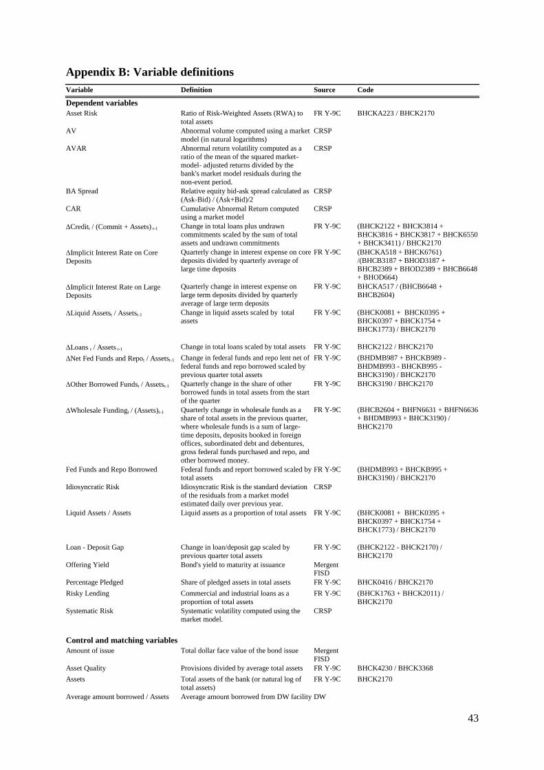
43

Appendix B: Variable definitions

Variable Definition Source Code

Dependent variables

Asset Risk Ratio of Risk-Weighted Assets (RWA) to

total assets

FR Y-9C BHCKA223 / BHCK2170

AV Abnormal volume computed using a market

model (in natural logarithms)

CRSP

AVAR Abnormal return volatility computed as a

ratio of the mean of the squared market-

model- adjusted returns divided by the bank's market model residuals during the

non-event period.

CRSP

BA Spread Relative equity bid-ask spread calculated as

(Ask-Bid) / (Ask+Bid)/2

CRSP

CAR Cumulative Abnormal Return computed using a market model

CRSP

Creditt / (Commit + Assets) t-1 Change in total loans plus undrawn

commitments scaled by the sum of total assets and undrawn commitments

FR Y-9C (BHCK2122 + BHCK3814 +

BHCK3816 + BHCK3817 + BHCK6550 + BHCK3411) / BHCK2170

Implicit Interest Rate on Core

Deposits

Quarterly change in interest expense on core

deposits divided by quarterly average of

large time deposits

FR Y-9C (BHCKA518 + BHCK6761)

/(BHCB3187 + BHOD3187 +

BHCB2389 + BHOD2389 + BHCB6648 + BHOD664)

Implicit Interest Rate on Large

Deposits

Quarterly change in interest expense on

large term deposits divided by quarterly

average of large term deposits

FR Y-9C BHCKA517 / (BHCB6648 +

BHCB2604)

Liquid Assetst / Assetst-1 Change in liquid assets scaled by total assets

FR Y-9C (BHCK0081 + BHCK0395 + BHCK0397 + BHCK1754 +

BHCK1773) / BHCK2170

Loans t / Assets t-1 Change in total loans scaled by total assets FR Y-9C BHCK2122 / BHCK2170

Net Fed Funds and Repot / Assetst-1 Change in federal funds and repo lent net of

federal funds and repo borrowed scaled by

previous quarter total assets

FR Y-9C (BHDMB987 + BHCKB989 -

BHDMB993 - BHCKB995 -

BHCK3190) / BHCK2170

Other Borrowed Fundst / Assetst-1 Quarterly change in the share of other

borrowed funds in total assets from the start

of the quarter

FR Y-9C BHCK3190 / BHCK2170

Wholesale Fundingt / (Assets)t-1 Quarterly change in wholesale funds as a share of total assets in the previous quarter,

where wholesale funds is a sum of large-

time deposits, deposits booked in foreign offices, subordinated debt and debentures,

gross federal funds purchased and repo, and

other borrowed money.

FR Y-9C (BHCB2604 + BHFN6631 + BHFN6636 + BHDMB993 + BHCK3190) /

BHCK2170

Fed Funds and Repo Borrowed Federal funds and report borrowed scaled by total assets

FR Y-9C (BHDMB993 + BHCKB995 + BHCK3190) / BHCK2170

Idiosyncratic Risk Idiosyncratic Risk is the standard deviation

of the residuals from a market model estimated daily over previous year.

CRSP

Liquid Assets / Assets Liquid assets as a proportion of total assets FR Y-9C (BHCK0081 + BHCK0395 +

BHCK0397 + BHCK1754 +

BHCK1773) / BHCK2170

Loan - Deposit Gap Change in loan/deposit gap scaled by

previous quarter total assets

FR Y-9C (BHCK2122 - BHCK2170) /

BHCK2170

Offering Yield Bond's yield to maturity at issuance Mergent FISD

Percentage Pledged Share of pledged assets in total assets FR Y-9C BHCK0416 / BHCK2170

Risky Lending Commercial and industrial loans as a

proportion of total assets

FR Y-9C (BHCK1763 + BHCK2011) /

BHCK2170

Systematic Risk Systematic volatility computed using the market model.

CRSP

Control and matching variables

Amount of issue Total dollar face value of the bond issue Mergent

FISD

Asset Quality Provisions divided by average total assets FR Y-9C BHCK4230 / BHCK3368

Assets Total assets of the bank (or natural log of

total assets)

FR Y-9C BHCK2170

Average amount borrowed / Assets Average amount borrowed from DW facility DW

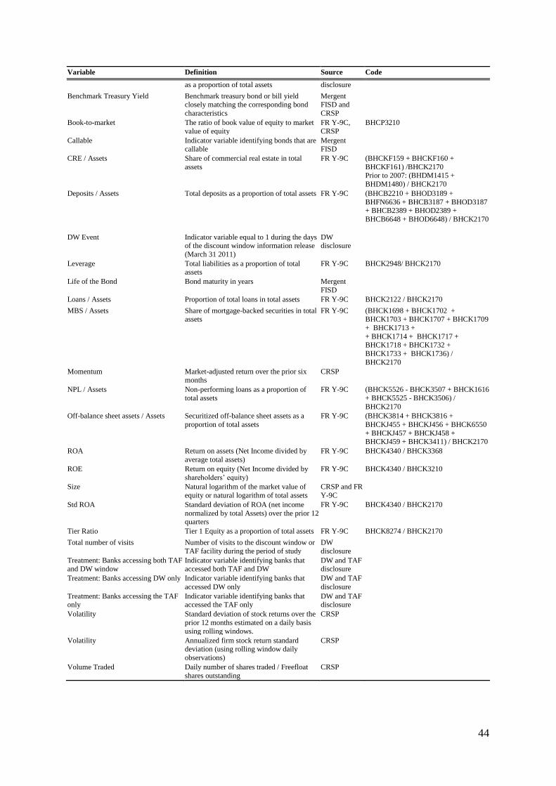
44

Variable Definition Source Code

as a proportion of total assets disclosure

Benchmark Treasury Yield Benchmark treasury bond or bill yield closely matching the corresponding bond

characteristics

Mergent FISD and

CRSP

Book-to-market The ratio of book value of equity to market

value of equity

FR Y-9C,

CRSP

BHCP3210

Callable Indicator variable identifying bonds that are callable

Mergent FISD

CRE / Assets Share of commercial real estate in total

assets

FR Y-9C (BHCKF159 + BHCKF160 +

BHCKF161) /BHCK2170 Prior to 2007: (BHDM1415 +

BHDM1480) / BHCK2170

Deposits / Assets Total deposits as a proportion of total assets FR Y-9C (BHCB2210 + BHOD3189 +

BHFN6636 + BHCB3187 + BHOD3187 + BHCB2389 + BHOD2389 +

BHCB6648 + BHOD6648) / BHCK2170

DW Event Indicator variable equal to 1 during the days of the discount window information release

(March 31 2011)

DW disclosure

Leverage Total liabilities as a proportion of total assets

FR Y-9C BHCK2948/ BHCK2170

Life of the Bond Bond maturity in years Mergent

FISD

Loans / Assets Proportion of total loans in total assets FR Y-9C BHCK2122 / BHCK2170

MBS / Assets Share of mortgage-backed securities in total assets

FR Y-9C (BHCK1698 + BHCK1702 + BHCK1703 + BHCK1707 + BHCK1709

+ BHCK1713 +

+ BHCK1714 + BHCK1717 + BHCK1718 + BHCK1732 +

BHCK1733 + BHCK1736) /

BHCK2170

Momentum Market-adjusted return over the prior six

months

CRSP

NPL / Assets Non-performing loans as a proportion of

total assets

FR Y-9C (BHCK5526 - BHCK3507 + BHCK1616

+ BHCK5525 - BHCK3506) /

BHCK2170

Off-balance sheet assets / Assets Securitized off-balance sheet assets as a

proportion of total assets

FR Y-9C (BHCK3814 + BHCK3816 +

BHCKJ455 + BHCKJ456 + BHCK6550

+ BHCKJ457 + BHCKJ458 + BHCKJ459 + BHCK3411) / BHCK2170

ROA Return on assets (Net Income divided by

average total assets)

FR Y-9C BHCK4340 / BHCK3368

ROE Return on equity (Net Income divided by

shareholders’ equity)

FR Y-9C BHCK4340 / BHCK3210

Size Natural logarithm of the market value of

equity or natural logarithm of total assets

CRSP and FR

Y-9C

Std ROA Standard deviation of ROA (net income

normalized by total Assets) over the prior 12 quarters

FR Y-9C BHCK4340 / BHCK2170

Tier Ratio Tier 1 Equity as a proportion of total assets FR Y-9C BHCK8274 / BHCK2170

Total number of visits Number of visits to the discount window or

TAF facility during the period of study

DW

disclosure

Treatment: Banks accessing both TAF and DW window

Indicator variable identifying banks that accessed both TAF and DW

DW and TAF disclosure

Treatment: Banks accessing DW only Indicator variable identifying banks that

accessed DW only

DW and TAF

disclosure

Treatment: Banks accessing the TAF only

Indicator variable identifying banks that accessed the TAF only

DW and TAF disclosure

Volatility Standard deviation of stock returns over the

prior 12 months estimated on a daily basis

using rolling windows.

CRSP

Volatility Annualized firm stock return standard deviation (using rolling window daily

observations)

CRSP

Volume Traded Daily number of shares traded / Freefloat

shares outstanding

CRSP

45

Appendix C: DW event coverage in the news

The table and figure below illustrate that the DW event was newsworthy. The entire universe of Factiva was searched for

news and then filtered to the news on the banking sector and the DW.

03/31/2011 03/31/2010 03/30/2012

Number of news stories on Factiva (no filters); global news 34,670 30,562 34,923

US news 8,050 8,188 3,678

US Banking sector 345 65 245

Discount window 164 0 0

Dow Jones News 862 809 690

US Banking sector 100 63 54

Discount window 80 0 0

0

200

400

600

800

1,000

1,200

Discount window

US Banking sector

Dow Jones News

03/31/2010 03/31/2011 03/30/2012

46

Table 1: Descriptive statistics

The tables below present summary statistics for the main dependent and control variables used in the analysis of the matched

sample. Panel A presents quarterly variables computed using quarterly data for the period of 2009Q2 to 2012Q3. Panel B

shows the main variables used for the equity bid-ask spread analysis over a shorter horizon of 2010Q3 to 2011Q3 (controls

are in natural logarithms at a monthly frequency). Panel C presents variables used for debt issuance analysis using the time

period of 2010Q3 to 2011Q3. Panel D presents the variables used in the propensity score estimation and the resulting

matched sample using the data for the period of 2004Q1 to 2006Q4. All observations apart from equity returns, bid-ask

spreads, abnormal volumes, and volatility are winsorized at the utmost 1% tails of their respective distributions to adjust for

the effects of extreme observations. Variables are defined in Appendix B. ***, **, * designate significance at 1%, 5% and 10%

levels respectively. T-statistics (reported in parenthesis) are estimated using the differences in means test.

Panel A: Matched quarterly sample

Variable N Mean SD P25 P50 P75

Asset Quality 3,017 0.006 0.007 0.001 0.003 0.009

Asset Risk 3,017 0.714 0.101 0.647 0.722 0.782

CI Loans / Assets 3,017 0.102 0.066 0.054 0.087 0.136

Credit t / (Commit + Assets) t-1 3,017 -0.002 0.041 -0.018 -0.005 0.008

Implicit Interest Rate on Core Deposits 3,017 -0.703 1.961 -0.347 0.270 0.365

Implicit Interest Rate on Large Deposits 3,017 -0.697 1.882 -0.173 0.263 0.362

Liquid Assets t / Assets t-1 3,017 0.008 0.033 -0.010 0.005 0.022

Loans t / Assets t-1 3,017 -0.001 0.039 -0.016 -0.004 0.007

Net Fed Funds and Repo t / Assets t-1 3,017 -0.001 0.008 -0.002 0.000 0.001

Other Borrowed Funds t / Assets t-1 3,017 -0.003 0.014 -0.006 0.000 0.000

Wholesale Funding t / (Assets) t-1 3,017 -0.011 0.035 -0.026 -0.009 0.008

Deposits / Assets 3,017 0.774 0.098 0.733 0.793 0.834

Idiosyncratic Risk 3,017 0.522 0.367 0.280 0.404 0.665

Liquid Assets / Assets 3,017 0.264 0.110 0.187 0.248 0.324

Loans / Assets 3,017 0.643 0.110 0.591 0.654 0.714

(Loans - Deposits ) / Assets 3,017 -0.133 0.123 -0.207 -0.126 -0.057

Log (Assets) 3,017 14.877 1.379 13.834 14.564 15.663

Net Federal Funds and Repo / Assets 3,017 0.030 0.034 0.002 0.019 0.046

Net Wholesale Funding / Assets 3,017 -0.193 0.125 -0.262 -0.186 -0.110

NPL / Assets 3,017 0.002 0.004 0.000 0.000 0.002

Off-balance sheets Assets/Assets 3,017 0.122 0.067 0.070 0.112 0.165

Other Borrowed Funds / Assets 3,017 0.060 0.055 0.019 0.047 0.085

Percentage of Assets Pledged 3,017 0.112 0.076 0.060 0.100 0.149

ROA 3,017 0.001 0.008 0.000 0.002 0.005

Systematic Risk 3,017 0.225 0.172 0.081 0.210 0.316

Tier Ratio 3,017 0.092 0.025 0.080 0.092 0.106

Volatility 3,017 0.600 0.358 0.374 0.485 0.727

Panel B: Variables used in the equity bid-ask spread analysis

Variable N Mean SD P25 P50 P75

BA Spread 3,724 0.029 0.036 0.004 0.013 0.041

Size 3,724 12.386 2.052 10.833 12.190 13.693

Volume Traded 3,724 0.372 1.413 -0.571 0.519 1.464

Volatility t-1 3,724 -0.407 0.447 -0.739 -0.378 -0.089

Panel C: Variables used in the cost of debt issuance analysis

Variable N Mean SD P25 P50 P75

Offering Yield (%) 1,077 12.064 5.189 9.000 11.950 15.200

Benchmark Treasury Yield (%) 1,077 0.621 1.008 0.169 0.264 0.354

Log (1+ Bond Life) 1,077 5.551 1.155 4.585 5.242 5.916

Log (Bond Amount of Issue) 1,077 6.944 2.025 5.665 6.597 8.085

Callable 1,077 0.023 0.148 0.000 0.000 0.000

Log (Assets) 1,077 20.522 1.440 18.137 21.474 21.511

Asset Risk (%) 1,077 52.931 5.137 49.578 53.353 54.640

Tier Ratio (%) 1,077 6.784 0.629 6.570 6.698 6.847

Deposits / Assets (%) 1,077 31.827 13.315 30.571 32.427 44.785

ROA (%) 1,077 0.333 0.286 0.035 0.253 0.585

Rating 1,077 5.219 0.660 5.000 5.000 5.000

47

Panel D: Variables used in propensity score matching (pre-matched and matched values)

Treatment: Banks accessing DW (full sample)

Variable N Mean SD P25 P50 P75 t-statistic

Assets (US$ bn) 197 8.5799 20.1000 0.6896 1.5667 4.5028 (2.1332) **

Tier Ratio 197 0.0876 0.0170 0.0757 0.0851 0.0961 (-0.9965)

Std ROA 197 0.0036 0.0014 0.0028 0.0034 0.0042 (0.6377)

CRE / Assets 197 0.2937 0.1377 0.1864 0.2794 0.3904 (0.5850)

MBS / Assets 197 0.1034 0.0822 0.0351 0.0893 0.1554 (0.4376)

ROE 197 0.0776 0.0295 0.0615 0.0784 0.0945 (5.7358) ***

Liquid Assets / Assets 197 0.2436 0.1159 0.1631 0.2263 0.2967 (-0.4322)

Leverage 197 0.9112 0.0188 0.9012 0.9136 0.9248 (1.5559)

Control Group: Banks that did not access DW (full sample)

Variable N Mean SD P25 P50 P75

Assets (US$ bn) 371 5.1389 14.3000 0.4455 0.8688 2.1518

Tier Ratio 371 0.0892 0.0187 0.0776 0.0861 0.0956

Std ROA 371 0.0035 0.0020 0.0025 0.0032 0.0039

CRE / Assets 371 0.2866 0.1354 0.1896 0.2741 0.3837

MBS / Assets 371 0.1002 0.0830 0.0343 0.0873 0.1433

ROE 371 0.0607 0.0394 0.0421 0.0663 0.0843

Liquid Assets / Assets 371 0.2480 0.1156 0.1637 0.2328 0.3181

Leverage 371 0.9083 0.0248 0.8969 0.9119 0.9255

Treatment: Banks accessing DW (matched sample)

Variable N Mean SD P25 P50 P75 t-statistic

Assets (US$ bn) 197 8.5799 20.1000 0.6896 1.5667 4.5028 (0.7319)

Tier Ratio 197 0.0876 0.0170 0.0757 0.0851 0.0961 (-0.4546)

Std ROA 197 0.0036 0.0014 0.0028 0.0034 0.0042 (-0.4739)

CRE / Assets 197 0.2937 0.1377 0.1864 0.2794 0.3904 (-0.1157)

MBS / Assets 197 0.1034 0.0822 0.0351 0.0893 0.1554 (0.1224)

ROE 197 0.0776 0.0295 0.0615 0.0784 0.0945 (0.0462)

Liquid Assets / Assets 197 0.2436 0.1159 0.1631 0.2263 0.2967 (-0.2308)

Leverage 197 0.9112 0.0188 0.9012 0.9136 0.9248 (-0.4693)

Control Group: Banks that did not access DW (matched sample)

Variable N Mean SD P25 P50 P75

Assets (US$ bn) 197 7.1902 17.5000 0.4934 1.0599 3.4572

Tier Ratio 197 0.0884 0.0184 0.0775 0.0855 0.0951

Std ROA 197 0.0037 0.0016 0.0028 0.0035 0.0041

CRE / Assets 197 0.2953 0.1485 0.1858 0.2817 0.4206

MBS / Assets 197 0.1024 0.0882 0.0318 0.0893 0.1432

ROE 197 0.0774 0.0293 0.0614 0.0802 0.0947

Liquid Assets / Assets 197 0.2464 0.1248 0.1597 0.2260 0.3118

Leverage 197 0.9121 0.0216 0.9022 0.9151 0.9281

48

Table 2: Event study results: Cumulative Abnormal Returns, Abnormal Volumes and Abnormal Returns Volatility (matched sample)

This table presents univariate and multivariate event study results using the matched sample. Treatment refers to banks that accessed the DW and Control refers to banks that did not access the

DW. Panel A shows the univariate comparisons for cumulative abnormal returns (CAR), abnormal volumes (AV) and abnormal return volatility (AVAR) over a short (0, +3) window computed

using the market model. The difference column shows the difference between control and sample banks. Panel B presents the short-window OLS estimation results of the cumulative abnormal

returns (CAR), abnormal volumes (AV) and abnormal volatility (AVAR) following the DW disclosures on March 31, 2011. The estimation period for the market model is 125 trading days prior

to the TAF event on December 1, 2010. Abnormal volume is calculated as ln( it i⁄ ), where it is the mean event-period volume for bank i and i is the mean estimation-period

volume measured over a period of 30 trading days before the TAF event. Abnormal return volatility is calculated as ln(uit i

⁄ ), where uit it - ( i i mt), it is bank i’s stock return,

mt is the value-weighted return for the US stock market and i and i are bank i’s estimation-period market model parameter estimates. i

is the variance of the market-model residuals in the

non-event period. All variables are presented in decimals and are computed as mean values over a four-day period following the DW disclosure event on March 31, 2011, including the event

date. Control banks are matched to the banks accessing the DW using propensity score matching based on the pre-crisis quarterly data for 2004Q1 to 2006Q4. All variables are defined in

Appendix B. ***, **, * designate significance at 1%, 5% and 10% levels respectively. T-statistics (reported in parenthesis) are computed based on robust standard errors. Inferences are similar

with bootstrapped p-values.

Panel A: Univariate cross-sectional tests following the DW disclosures

Control sample:

Other banks

Treatment sample:

Banks accessing DW Difference

Variable Days Mean t-statistic Mean t-statistic Mean t-statistic

CAR 4 0.0010 (0.411) 0.0105*** (4.188) 0.0095* (1.871)

AV 4 -0.2241** (-2.578) -0.4464*** (-6.752) -0.2222** (-2.037)

AVAR 4 -9.0894*** (-32.553) -9.0885*** (-52.483) 0.0009 (0.003)

49

Panel B: Multivariate cross-sectional tests following the DW disclosures

This table presents the short-window (0, +3) OLS estimation results of the cumulative abnormal returns (CAR), abnormal volumes (AV) and abnormal volatility (AVAR) following the DW

disclosures on March 31, 2011.

CAR CAR CAR CAR CAR AV AV AVAR AVAR

(1) (2) (3) (4) (5) (6) (7) (8) (9)

Treatment: Banks accessing DW 0.0095* 0.0096* 0.0110**

-0.2607**

0.0364

(1.873) (1.829) (2.041)

(-2.262)

(0.104)

Treatment: Banks accessing DW only

0.0070 0.0079

-0.3495***

0.1155

(1.239) (1.398)

(-2.674)

(0.310)

Treatment: Banks accessing TAF only

-0.0017 -0.0016

-0.1959

-0.0613

(-0.116) (-0.109)

(-1.283)

(-0.070)

Treatment: Banks accessing both DW and TAF

0.0157** 0.0200***

-0.0514

-0.0137

(2.191) (2.648)

(-0.340)

(-0.026)

Size

-0.0002 -0.0000 -0.0009 -0.0011 -0.0260 -0.0507 -0.0502 -0.0356

(-0.068) (-0.017) (-0.377) (-0.469) (-0.804) (-1.491) (-0.502) (-0.318)

Book-to-Market

-0.0032 -0.0032 -0.0031 -0.0031 -0.0135 -0.0125 -0.0068 -0.0070

(-1.396) (-1.398) (-1.454) (-1.497) (-0.391) (-0.375) (-0.079) (-0.082)

Momentum

-1.2176 -1.2158 -1.1827 -1.1988 1.4795 2.5648 59.5014 58.5385

(-0.804) (-0.817) (-0.784) (-0.818) (0.034) (0.060) (0.653) (0.643)

Leverage

-0.0539 -0.0550 -0.0679 -0.0756 1.0119 0.4251 -5.2141 -5.1261

(-0.373) (-0.382) (-0.469) (-0.528) (0.420) (0.180) (-0.840) (-0.799)

Average amount borrowed / Assets

-0.0016*

-0.0016*

-0.0501* -0.0354 -0.0219 0.0252

(-1.967)

(-1.894)

(-1.874) (-1.407) (-0.849) (0.352)

Total number of visits

-0.0001**

-0.0001*** 0.0038* 0.0026

-0.0034

(-2.524)

(-3.012) (1.830) (1.358)

(-0.584)

Intercept 0.0010 0.0562 0.0024 0.0782 0.0876 -0.8082 0.0376 -3.7567 -4.0048

(0.216) (0.385) (0.098) (0.528) (0.598) (-0.342) (0.016) (-0.607) (-0.617)

Observations 250 250 250 250 250 250 250 250 250

Adjusted R-squared 0.012 0.027 0.030 0.026 0.037 0.010 0.018 -0.016 -0.026

50

Table 3: Univariate difference-in-difference tests of main dependent variables

This table presents univariate comparison between Treated banks (banks that accessed the DW) and Control banks (banks that did not access the DW) for all dependent variables used in this

paper. The difference column shows the difference between control and sample banks. Control banks are matched to the banks accessing the DW using propensity score matching based on the

pre-crisis quarterly data for 2004Q1 to 2006Q4. All variables are defined in Appendix B. ***, **, * designate significance at 1%, 5% and 10% levels respectively. T-statistics (reported in

parenthesis) are computed based on robust standard errors.

Before DW Disclosures After DW Disclosures Difference - in - Differences

Control Treated Difference t-statistic Control Treated Difference t-statistic

t-statistic

Variable (1) (2) (3) = (2) - (1) (4) (5) (6) (7) = (6) - (5) (8) (9) = (7) - (3) (10)

BA Spread (long horizon) -4.047 -4.536 -0.489 (-7.56)*** -4.180 -4.678 -0.498 (-4.86)*** -0.009 (-0.09)

BA Spread (short horizon) -4.312 -4.762 -0.450 (-3.89)*** -4.326 -4.806 -0.480 (-5.29)*** -0.030 (-0.2)

Offering bond yield 13.557 10.613 -2.944 (-12.75)*** 10.466 6.450 -4.016 (11.2)*** -1.072 (3.04)***

Idiosyncratic Risk 0.602 0.641 0.039 (2.08)** 0.426 0.395 -0.031 (-3.52)*** -0.070 (-2.58)***

Systematic Risk 0.208 0.260 0.052 (5.72)*** 0.180 0.218 0.038 (-2.38)*** -0.014 (-1.08)

Asset Risk 0.721 0.733 0.012 (2.4)*** 0.681 0.704 0.023 (4.24)*** 0.011 (1.49)

Risky Lending 0.094 0.106 0.012 (3.71)*** 0.089 0.108 0.019 (3)*** 0.007 (1.22)

Liquid Assets 0.252 0.245 -0.007 (-1.37) 0.292 0.277 -0.015 (-1.82)* -0.008 (-0.88)

Pct. Pledged 0.104 0.115 0.011 (2.81)*** 0.111 0.113 0.002 (-2.04)** -0.009 (-1.48)

Fed Funds and Repo Borrowed 0.028 0.033 0.005 (3.35)*** 0.028 0.029 0.001 (-2.33)*** -0.004 (-1.69)*

Loan - Deposit Gap -0.121 -0.102 0.019 (3.02)*** -0.170 -0.148 0.022 (9.14)*** 0.003 (0.26)

Liquid Assetst / Assetst-1 0.013 0.007 -0.006 (-3.43)*** 0.007 0.007 0.000 (5.41)*** 0.006 (2.27)**

Loanst / Assetst-1 -0.001 -0.005 -0.004 (-2.13)** 0.000 0.004 0.004 (3.83)*** 0.008 (2.78)***

Creditt / (Commit + Assets)t-1 -0.003 -0.007 -0.004 (-2)** 0.000 0.004 0.004 (3.91)*** 0.008 (2.83)***

Net Fed Funds and Repot / Assetst-1 0.000 -0.001 -0.001 (-2.23)** -0.001 0.000 0.001 (2.31)** 0.002 (1.67)*

Other Borrowed Fund t / Assetst-1 -0.003 -0.004 -0.001 (-1.09) -0.002 -0.001 0.001 (1.58) 0.002 (1.14)

Wholesale Fundingt /Assetst-1 -0.016 -0.012 0.004 (2.35)*** -0.009 -0.008 0.001 (-1.76)* -0.003 (-1.27)

Implicit Interest Rate on Large Deposits -0.514 -0.489 0.025 (0.26) -0.869 -0.939 -0.070 (-0.92) -0.095 (-0.68)

Implicit Interest Rate on Core Deposits -0.419 -0.397 0.022 (0.22) -1.065 -1.011 0.054 (0.33) 0.032 (0.22)

51

Table 4: Cost of capital: daily equity bid-ask spreads (matched sample)

This table presents the difference-in-difference estimation results of the impact on the cost of capital as measured by the adverse selection component of the bid-ask spread using the matched

sample.

prea it

entt

reate i

entt reate i

i ei,t

olumei,t

olatilit

i,t ∑

nn

ontrolsit it

where BA Spreadit is the natural logarithm of the relative equity bid-ask spread for each bank deflated by the average price, Eventt is an indicator variable for the window following the

disclosure of the DW information. Treatedi refers to indicator variables for each category of banks accessing the DW or TAF (DW only access, TAF only access and DW and TAF). Sizei,t-1 is

the natural logarithm of daily market capitalization of each bank to take into account the size of the bank, Volumei,t-1 is the volume of shares trading as a proportion of the shares outstanding, and

Volatilityi,t-1 is the rolling standard deviation of daily stock returns in the previous trading year. The treatment effect is captured by the coefficient 3 on the difference-in-differences estimator.

Columns (1) and (2) present the results for all banks in the matched sample. Columns (3) and (4) provide results for the banks in the top quartile of average DW borrowing as a proportion of

total assets. Banks in columns (5) and (6) are in the top quartile of borrowers by frequency. Finally columns (7) and (8) show the results for banks with negative abnormal returns on the DW

disclosure event. All other variables are defined in Appendix B; ***, **, * designate significance at 1%, 5% and 10% levels respectively. T-statistics (reported in parenthesis) are computed

based on robust standard errors clustered at the BHC level. Inferences remain unchanged using bootstrapped p-values. Control banks are matched to the banks accessing the DW using

propensity score matching based on the pre-crisis quarterly data for 2004Q1 to 2006Q4. The regression is estimated using daily values over a seven-day period around the DW disclosure event

on March 31, 2011, to match the cross-section market tests on the (0,+3) window.

All banks

Top quartile DW Borrowers

(by amount)

Top quartile DW Borrowers

(by frequency)

Banks with negative CARs on

DW Disclosure Event

(1) (2) (3) (4) (5) (6) (7) (8)

Treatment: Banks accessing DW -0.0661

-0.0118

(-0.858)

(-0.090)

DW Event 0.1183** 0.1594*** 0.0769 0.0890 0.0758 0.0132 0.1128 0.1404**

(2.556) (3.289) (1.007) (1.565) (1.103) (0.082) (1.590) (2.122)

Banks accessing DW * DW Event -0.0522

-0.1493*

(-0.957)

(-1.668)

Treatment: Banks accessing DW only

-0.0399

0.5115**

0.3605*

0.0838

(-0.494)

(2.309)

(1.802)

(0.650)

Banks accessing DW only * DW Event

-0.1115*

-0.0542

-0.2123**

(-1.748)

(-0.389)

(-2.218)

Treatment: Banks accessing TAF only

0.0184

-0.0375

(0.123)

(-0.152)

Banks accessing TAF only * DW Event

-0.3691***

-0.3881

(-2.817)

(-1.645)

Treatment: Banks accessing both DW and TAF

-0.1551

-0.7117**

(-1.101)

(-2.297)

Banks accessing both DW and TAF * DW Event

-0.0575

0.0937

-0.0850

(-1.003)

(0.565)

(-0.997)

Sizet-1 -0.4620*** -0.4491*** -0.5153*** -0.4724*** -0.4967*** -0.4677*** -0.4237*** -0.3723***

(-10.203) (-8.538) (-8.506) (-10.286) (-11.206) (-11.718) (-6.754) (-5.891)

Volume traded t-1 -0.3610*** -0.3598*** -0.3541*** -0.3123*** -0.3505*** -0.3291*** -0.3131*** -0.2785***

(-7.495) (-7.153) (-5.427) (-4.248) (-5.376) (-4.725) (-5.204) (-5.465)

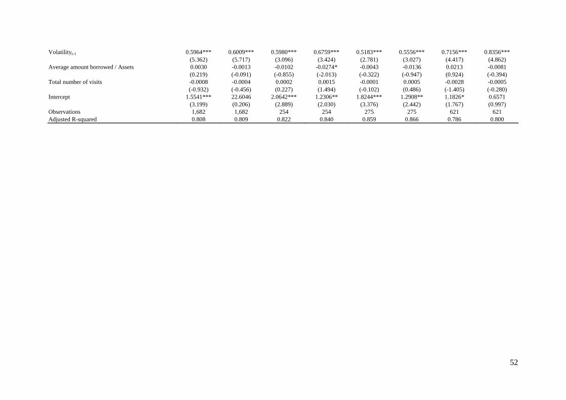
52

Volatilityt-1 0.5964*** 0.6009*** 0.5980*** 0.6759*** 0.5183*** 0.5556*** 0.7156*** 0.8356***

(5.362) (5.717) (3.096) (3.424) (2.781) (3.027) (4.417) (4.862)

Average amount borrowed / Assets 0.0030 -0.0013 -0.0102 -0.0274* -0.0043 -0.0136 0.0213 -0.0081

(0.219) (-0.091) (-0.855) (-2.013) (-0.322) (-0.947) (0.924) (-0.394)

Total number of visits -0.0008 -0.0004 0.0002 0.0015 -0.0001 0.0005 -0.0028 -0.0005

(-0.932) (-0.456) (0.227) (1.494) (-0.102) (0.486) (-1.405) (-0.280)

Intercept 1.5541*** 22.6046 2.0642*** 1.2306** 1.8244*** 1.2908** 1.1826* 0.6571

(3.199) (0.206) (2.889) (2.030) (3.376) (2.442) (1.767) (0.997)

Observations 1,682 1,682 254 254 275 275 621 621

Adjusted R-squared 0.808 0.809 0.822 0.840 0.859 0.866 0.786 0.800

53

Table 5: Cost of capital: monthly equity bid-ask spreads (matched sample)

This table presents the difference-in-difference estimation results of the impact on the cost of capital as measured by the adverse selection component of the bid-ask spread using the matched

sample.

prea it

entt reate i

i ei,t

olumei,t

olatilit

i,t ∑

nn

ontrolsit t i it

where BA Spreadit is the natural logarithm of the monthly median relative equity bid-ask spread for each bank deflated by the average price, Event is an indicator variable for the window

following the disclosure of the DW information. Eventt x Treatedi refers to the interaction that takes the value of one for banks that access the DW and the effect of this information post-

disclosure of March 31, 2011. This is the difference-in-difference estimator. Sizei,t-1 is the natural logarithm of daily market capitalization of each bank to take into account the size of the bank,

Volumei,t-1 is the volume of shares trading as a proportion of the shares outstanding, and Volatilityi,t-1 is the rolling standard deviation of daily stock returns in the previous trading year. Tt reflects

the year and month fixed effects and Bi refers to the holding company fixed effects. The treatment effect is captured by the coefficient 1 on the difference-in-differences estimator. This analysis

uses bank and time fixed effects and therefore only the difference-in-differences operator is identified. Columns (1) and (2) present the results for all banks in the matched sample. Columns (3)

and (4) provide results for the banks in the top quartile of average DW borrowing as a proportion of total assets. Banks in columns (5) and (6) are in the top quartile of borrowers by frequency.

Finally columns (7) and (8) show the results for banks with negative abnormal returns on the DW disclosure event. Variables are defined in Appendix B; ***, **, * designate significance at 1%,

5% and 10% levels respectively. T-statistics (reported in parenthesis) are computed based on robust standard errors clustered at the BHC level. Inferences remain unchanged using bootstrapped

p-values. Control banks are matched to the banks accessing the DW using propensity score matching based on the pre-crisis quarterly data for 2004Q1 to 2006Q4. The regression is estimated

using monthly medians of daily relative bid-ask spread values over a five-quarter period following the passage of the Dodd-Frank Act from 2010Q3 to 2011Q3.

All banks Top quartile DW Borrowers

(by amount)

Top quartile DW Borrowers

(by frequency)

Banks with negative CARs on

DW Disclosure Event

(1) (2) (3) (4) (5) (6) (7) (8)

Banks accessing DW * DW Event 0.0677* 0.0125 0.0233 0.1250**

(1.804) (0.092) (0.153) (2.042)

Banks accessing DW only * DW Event 0.0805* 0.0588 0.0360 0.1636**

(1.909) (0.428) (0.237) (2.517)

Banks accessing TAF only * DW Event -0.0001 0.1354

(-0.001) (1.535)

Banks accessing both DW and TAF * DW Event 0.0414 -0.0637 0.0002 0.0526

(0.830) (-0.476) (0.001) (0.491)

Sizet-1 -0.0375 -0.0389 0.0099 0.0076 -0.0097 -0.0104 -0.0196 -0.0236

(-1.314) (-1.388) (0.190) (0.148) (-0.181) (-0.195) (-0.617) (-0.795)

Volumet-1 -0.1246*** -0.1247*** -0.1080*** -0.1035*** -0.1302*** -0.1289*** -0.1097*** -0.1082***

(-6.694) (-6.694) (-3.008) (-2.836) (-3.277) (-3.121) (-3.916) (-3.874)

Volatilityt-1 0.1260* 0.1145* -0.0587 -0.0817 -0.0514 -0.0647 0.0230 -0.0021

(1.912) (1.679) (-0.299) (-0.429) (-0.254) (-0.306) (0.219) (-0.019)

Time fixed effects Yes Yes Yes Yes Yes Yes Yes Yes

Bank fixed effects Yes Yes Yes Yes Yes Yes Yes Yes

Observations 3,724 3,724 565 565 605 605 1,415 1,415

Adjusted R-squared 0.311 0.311 0.316 0.324 0.283 0.282 0.308 0.311

54

Table 6: Cost of capital: bond offering yields (matched sample)

This table presents the estimation results of the impact of the DW disclosures on banks’ cost of borrowing in the bond

market.

iel it entt reate i ∑ l ontrolsitl

t i it

The dependent variable is the bond-offering yield, which is measured as the bond’s yield to maturity at the time of issuance.

Benchmark Treasury Yield is the yield to maturity of a corresponding US Treasury bill or bond matched to each bond in the

sample on maturity and coupon. Bond Life is the bond maturity in years. Amount of Issue is the total dollar amount of the

face value of each bond at issuance. Callable is an indicator variable, which takes the value of one if the bond is callable and

zero otherwise. Assets are the total assets of each bank. Asset Risk is the share of risk-weighted assets in total assets, which

measures the overall riskiness of a bank’s assets. Tier Ratio is the share of Tier 1 capital in total assets. Deposits / Assets is

the ratio of banks’ total deposits to total assets. ROA measures each bank’s return on assets. Eventt x Treatedi takes the value

of one for bonds issued after the DW disclosure event on March 31, 2011, by banks that have accessed the DW (or TAF and

DW). Rating is a numerical credit rating for which the lowest value implies higher credit quality. Control banks are matched

to the banks accessing the DW using propensity score matching based on the pre-crisis quarterly data for 2004Q1 to

2006Q4. Tt captures the quarterly fixed effects and Bi captures the holding company fixed effects. This analysis uses bank-

and time- fixed effects and therefore only the difference-in-differences operator is identified. All continuous variables are in

percent and are winsorized at the utmost 1% tails of their respective distributions to adjust for the effects of extreme

observations. The regression is estimated over a five-quarter period following the passage of the Dodd-Frank Act from

2010Q3 to 2011Q3. All other variables are defined in Appendix B. ***, **, * designate significance at 1%, 5% and 10%

levels respectively. T-statistics (reported in parenthesis) are computed based on robust standard errors clustered at the BHC

level.

(1) (2)

Banks accessing DW * DW Event -1.1595*

(-1.869)

Banks accessing DW only * DW Event -1.8945**

(-1.967)

Banks accessing both DW and TAF * DW Event -0.1568

(-0.133)

Benchmark Treasury Yield 2.1716*** 2.1592***

(8.816) (8.755)

Log (1+ Bond Life) -3.7870*** -3.7795***

(-18.154) (-18.106)

Log (Bond Amount of Issue) -0.3889*** -0.3900***

(-5.745) (-5.760)

Callable -1.4117** -1.3909**

(-2.551) (-2.512)

Log (Assets) -4.8050 0.6762

(-0.307) (0.041)

Asset Risk -0.6619** -0.4134

(-2.392) (-1.110)

Tier Ratio -1.3991* -3.0201*

(-1.939) (-1.699)

Deposits / Assets 0.3720 0.1456

(1.469) (0.428)

ROA -1.3164 -0.8208

(-1.167) (-0.666)

Rating -0.3967 -0.4169

(-0.749) (-0.786)

Time fixed effects Yes Yes

Bank fixed effects Yes Yes

Observations 1,077 1,077

Adjusted R-squared 0.636 0.636

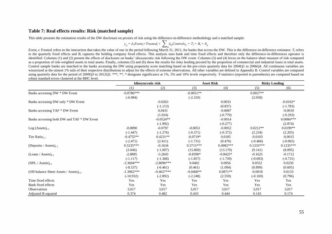
55

Table 7: Real effects results: Risk (matched sample)

This table presents the estimation results of the DW disclosure on proxies of risk using the difference-in-difference methodology and a matched sample:

it entt reate i ∑ m ontrolsit

m

t i it

Eventt x Treatedi refers to the interaction that takes the value of one in the period following March 31, 2011, for banks that access the DW. This is the difference-in-difference estimator. Tt refers

to the quarterly fixed effects and Bi captures the holding company fixed effects. This analysis uses bank and time fixed effects and therefore only the difference-in-differences operator is

identified. Columns (1) and (2) present the effects of disclosure on banks’ idiosyncratic risk following the DW event. Columns (3) and (4) focus on the balance sheet measure of risk computed

as a proportion of risk-weighted assets in total assets. Finally, columns (5) and (6) show the results for risky lending proxied by the proportion of commercial and industrial loans in total assets.

Control sample banks are matched to the banks accessing the DW using propensity score matching based on the pre-crisis quarterly data for 2004Q1 to 2006Q4. All continuous variables are

winsorized at the utmost 1% tails of their respective distributions to adjust for the effects of extreme observations. All other variables are defined in Appendix B. Control variables are computed

using quarterly data for the period of 2009Q3 to 2012Q3. ***, **, * designate significance at 1%, 5% and 10% levels respectively. T-statistics (reported in parenthesis) are computed based on

robust standard errors clustered at the BHC level.

Idiosyncratic risk Asset Risk Risky Lending

(1) (2) (3) (4) (5) (6)

Banks accessing DW * DW Event -0.0786***

-0.0051**

0.0027**

(-6.984)

(-2.310)

(2.058)

Banks accessing DW only * DW Event

-0.0263

0.0033

-0.0102*

(-1.113)

(0.837)

(-1.783)

Banks accessing TAF * DW Event

0.0431

-0.0087

-0.0010

(1.024)

(-0.779)

(-0.293)

Banks accessing both DW and TAF * DW Event

-0.0524**

-0.0014

0.0084***

(-1.992)

(-0.277)

(2.874)

Log (Assets)t-1 -0.0890 -0.0797 -0.0053 -0.0052 0.0212** 0.0199**

(-1.447) (-1.276) (-0.371) (-0.372) (2.234) (2.203)

Tier Ratiot-1 -0.4755** 0.4231** -0.0719* 0.0185 -0.0103 -0.0015

(-2.471) (2.411) (-1.731) (0.470) (-0.466) (-0.065)

(Deposits / Assets)t-1 0.5235*** -0.1634 0.5715*** 0.4982*** 0.1333*** 0.1235***

(3.046) (-1.007) (15.869) (13.170) (9.141) (8.095)

(Loans / Assets)t-1 -2.8885 -3.2643 -0.8390* -0.8425* -0.1625 -0.1712

(-1.117) (-1.368) (-1.857) (-1.739) (-0.693) (-0.731)

(NPL / Assets)t-1 -3.3694*** -2.8096*** 0.0402 0.0956 0.0352 0.0250

(-8.537) (-6.461) (0.461) (1.094) (0.899) (0.605)

(Off-balance Sheet Assets / Assets)t-1 -1.3962*** -0.4627*** -0.0460** 0.0871** -0.0018 0.0133

(-10.932) (-2.892) (-2.248) (2.559) (-0.169) (0.796)

Time fixed effects Yes Yes Yes Yes Yes Yes

Bank fixed effects Yes Yes Yes Yes Yes Yes

Observations 3,017 3,017 3,017 3,017 3,017 3,017

Adjusted R-squared 0.374 0.482 0.410 0.444 0.143 0.174

56

Table 8: Real effects results: Liquidity (matched sample)

This table presents the estimation results of the DW disclosure on proxies of liquidity using the difference-in-difference methodology and a matched sample:

it entt reate i ∑ m ontrolsit

m

t i it

Eventt x Treatedi refers to the interaction that takes the value of one in the period following March 31, 2011, for banks that access the DW. This is the difference-in-difference estimator. This

analysis uses bank and time fixed effects and therefore only the difference-in-differences operator is identified. Columns (1) and (2) present the effects of disclosure on banks’ balance sheet

liquidity measured as a proportion of liquid assets in total assets. Columns (3) and (4) show the results for the proportion of pledged assets in total assets as a measure of collateralized borrowing.

Columns (5) and (6) present the results for net borrowed Federal Funds and Repos as a proportion of total assets as a proxy for banks’ access to the federal funds market. Columns (7) and (8)

present the loan-deposit funding gap as a proportion of total assets as a proxy for a liquidity shortfall. Tt refers to the quarterly fixed effects and Bi is the holding company fixed effects. All other

variables are defined in Appendix B. Control variables are computed using quarterly data for the period of 2009Q3 to 2012Q3. Control sample banks are matched to the banks accessing the DW

using propensity score matching based on the pre-crisis quarterly data for 2004Q1 to 2006Q4. All continuous variables are winsorized at the utmost 1% tails of their respective distributions to

adjust for the effects of extreme observations. ***, **, * designate significance at 1%, 5% and 10% levels respectively. T-statistics (reported in parenthesis) are computed based on robust

standard errors clustered at the BHC level.

Liquid Assets Pct. Pledged Fed Funds and Repo Borrowed Loan - Deposit Gap

(1) (2) (3) (4) (5) (6) (7) (8)

Banks accessing DW * DW Event 0.0068***

-0.0057***

-0.0021**

-0.0113***

(3.969)

(-3.063)

(-2.207)

(-5.346)

Banks accessing DW only * DW Event

-0.0017

-0.0110***

-0.0031*

-0.0049

(-0.567)

(-2.893)

(-1.864)

(-1.469)

Banks accessing TAF * DW Event

-0.0014

0.0001

-0.0065*

-0.0050

(-0.135)

(0.008)

(-1.763)

(-0.405)

Banks accessing both DW and TAF * DW Event

-0.0038

-0.0023

-0.0029

0.0011

(-1.121)

(-0.491)

(-1.351)

(0.259)

Log (Assets)t-1 -0.0337*** -0.0378*** -0.0082 -0.0071 -0.0088** -0.0080** 0.0440*** 0.0465***

(-4.240) (-4.520) (-1.005) (-0.916) (-2.428) (-2.230) (4.836) (4.933)

Tier Ratiot-1 0.0761 0.0334 0.0619 0.0743 -0.0270 -0.0223 -0.0980 -0.0537

(1.202) (0.498) (0.772) (0.946) (-1.047) (-0.911) (-1.288) (-0.659)

(Deposits / Assets)t-1 0.0441* 0.0191 -0.1198*** -0.0941** -0.1057*** -0.1032*** -0.6873*** -0.6333***

(1.663) (0.684) (-3.497) (-2.495) (-5.471) (-5.220) (-17.935) (-15.109)

(Loans / Assets)t-1 -0.7041*** -0.6884*** -0.1354*** -0.1569*** -0.0111 -0.0111 0.6793*** 0.6371***

(-23.710) (-22.390) (-4.900) (-5.310) (-1.149) (-1.084) (16.766) (14.757)

(NPL / Assets)t-1 -1.2635*** -1.2041*** -0.4219 -0.4871* -0.1916 -0.2017 0.7270 0.6937

(-2.915) (-2.722) (-1.534) (-1.755) (-1.069) (-1.158) (1.029) (0.959)

(Off-balance Sheet Assets / Assets)t-1 -0.0053 -0.0155 -0.0086 0.0162 -0.0052 -0.0118 0.0032 0.0577**

(-0.312) (-0.598) (-0.622) (0.731) (-0.707) (-1.006) (0.163) (2.112)

Time fixed effects Yes Yes Yes Yes Yes Yes Yes Yes

Bank fixed effects Yes Yes Yes Yes Yes Yes Yes Yes

Observations 3,017 3,017 3,017 3,017 3,017 3,017 3,017 3,017

Adjusted R-squared 0.556 0.568 0.070 0.089 0.118 0.123 0.557 0.571

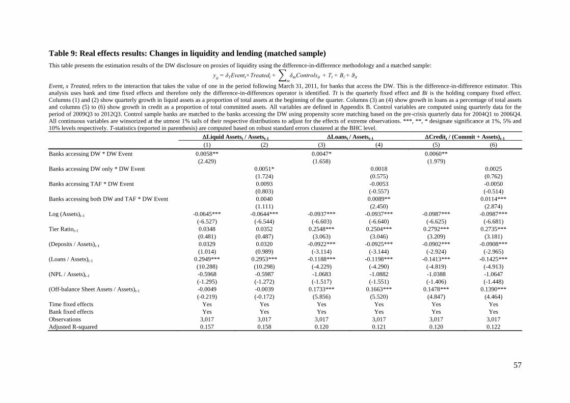
57

Table 9: Real effects results: Changes in liquidity and lending (matched sample)

This table presents the estimation results of the DW disclosure on proxies of liquidity using the difference-in-difference methodology and a matched sample:

it entt reate i ∑ m ontrolsit

m

t i it

Eventt x Treatedi refers to the interaction that takes the value of one in the period following March 31, 2011, for banks that access the DW. This is the difference-in-difference estimator. This

analysis uses bank and time fixed effects and therefore only the difference-in-differences operator is identified. Tt is the quarterly fixed effect and Bi is the holding company fixed effect.

Columns (1) and (2) show quarterly growth in liquid assets as a proportion of total assets at the beginning of the quarter. Columns (3) an (4) show growth in loans as a percentage of total assets

and columns (5) to (6) show growth in credit as a proportion of total committed assets. All variables are defined in Appendix B. Control variables are computed using quarterly data for the

period of 2009Q3 to 2012Q3. Control sample banks are matched to the banks accessing the DW using propensity score matching based on the pre-crisis quarterly data for 2004Q1 to 2006Q4.

All continuous variables are winsorized at the utmost 1% tails of their respective distributions to adjust for the effects of extreme observations. ***, **, * designate significance at 1%, 5% and

10% levels respectively. T-statistics (reported in parenthesis) are computed based on robust standard errors clustered at the BHC level.

Liquid Assetst / Assetst-1 Loanst / Assetst-1 Creditt / (Commit + Assets)t-1

(1) (2) (3) (4) (5) (6)

Banks accessing DW * DW Event 0.0058**

0.0047*

0.0060**

(2.429)

(1.658)

(1.979)

Banks accessing DW only * DW Event

0.0051*

0.0018

0.0025

(1.724)

(0.575)

(0.762)

Banks accessing TAF * DW Event

0.0093

-0.0053

-0.0050

(0.803)

(-0.557)

(-0.514)

Banks accessing both DW and TAF * DW Event

0.0040

0.0089**

0.0114***

(1.111)

(2.450)

(2.874)

Log (Assets)t-1 -0.0645*** -0.0644*** -0.0937*** -0.0937*** -0.0987*** -0.0987***

(-6.527) (-6.544) (-6.603) (-6.640) (-6.625) (-6.681)

Tier Ratiot-1 0.0348 0.0352 0.2548*** 0.2504*** 0.2792*** 0.2735***

(0.481) (0.487) (3.063) (3.046) (3.209) (3.181)

(Deposits / Assets)t-1 0.0329 0.0320 -0.0922*** -0.0925*** -0.0902*** -0.0908***

(1.014) (0.989) (-3.114) (-3.144) (-2.924) (-2.965)

(Loans / Assets)t-1 0.2949*** 0.2953*** -0.1188*** -0.1198*** -0.1413*** -0.1425***

(10.288) (10.298) (-4.229) (-4.290) (-4.819) (-4.913)

(NPL / Assets)t-1 -0.5968 -0.5987 -1.0683 -1.0882 -1.0388 -1.0647

(-1.295) (-1.272) (-1.517) (-1.551) (-1.406) (-1.448)

(Off-balance Sheet Assets / Assets)t-1 -0.0049 -0.0039 0.1733*** 0.1663*** 0.1478*** 0.1390***

(-0.219) (-0.172) (5.856) (5.520) (4.847) (4.464)

Time fixed effects Yes Yes Yes Yes Yes Yes

Bank fixed effects Yes Yes Yes Yes Yes Yes

Observations 3,017 3,017 3,017 3,017 3,017 3,017

Adjusted R-squared 0.157 0.158 0.120 0.121 0.120 0.122

58

Table 10: Real effects results: Changes in access to funding and funding costs (matched sample)

This table presents the estimation results of the DW disclosure on proxies of liquidity using the difference-in-difference methodology and a matched sample:

it entt reate i ∑ m ontrolsit

m

t i it

Eventt x Treatedi refers to the interaction that takes the value of one in the period following March 31, 2011, for banks that access the DW. This is the difference-in-difference estimator. This

analysis uses bank and time fixed effects and therefore only the difference-in-differences operator is identified. Tt refers to the quarterly fixed effects and Bi to the holding company fixed effects.

Columns (1) and (2) show quarterly changes in net federal funds and repo borrowing as a proportion of total assets at the beginning of the quarter. Columns (3) and (4) show growth in other

borrowed funds as a proportion of total assets. Columns (5) and (6) show growth in net wholesale funding as a proportion of total assets. Finally, columns (7) through (10) show the quarterly

change in the implicit interest rate banks pay on large and core deposits. All other variables are defined in Appendix B. Control variables are computed using quarterly data for the period of

2009Q3 to 2012Q3. Control sample banks are matched to the banks accessing the DW using propensity score matching based on the pre-crisis quarterly data for 2004Q1 to 2006Q4. All

continuous variables are winsorized at the utmost 1% tails of their respective distributions to adjust for the effects of extreme observations. ***, **, * designate significance at 1%, 5% and 10%

levels respectively. T-statistics (reported in parenthesis) are computed based on robust standard errors clustered at the BHC level.

Net Fed Funds and

Repot / Assetst-1

Other Borrowed Fundst

/ Assetst-1

Wholesale Fundingt /

Assetst-1

Implicit Interest Rate on

Large Deposits

Implicit Interest Rate on

Core Deposits

(1) (2) (3) (4) (5) (6) (7) (8) (9) (10)

Banks accessing DW * DW Event 0.0006

0.0005

-0.0027

-0.0984**

-0.0236

(1.183)

(0.503)

(-0.937)

(-2.136)

(-0.584)

Banks accessing DW only * DW Event

0.0002

-0.0004

-0.0049*

-0.1173**

0.0092

(0.325)

(-0.432)

(-1.655)

(-2.260)

(0.202)

Banks accessing TAF * DW Event

-0.0013

0.0008

-0.0091

-0.1991***

0.1327

(-0.709)

(0.409)

(-0.834)

(-2.709)

(1.365)

Banks accessing both DW and TAF * DW Event

0.0012

0.0025

-0.0007

-0.1164**

-0.0520

(1.649)

(1.519)

(-0.183)

(-1.975)

(-0.988)

Log (Assets)t-1 -0.0017 -0.0017 -0.0106*** -0.0106*** 0.0550*** 0.0550*** 0.3880*** 0.3873*** 0.2713** 0.2714**

(-1.234) (-1.249) (-2.762) (-2.803) (5.897) (5.889) (3.264) (3.250) (2.472) (2.478)

Tier Ratiot-1 0.0489*** 0.0483*** 0.1338*** 0.1318*** 0.1128 0.1104 2.8943** 2.9014** 0.2660 0.3012

(3.869) (3.821) (4.047) (3.984) (1.570) (1.535) (2.250) (2.249) (0.240) (0.270)

(Deposits / Assets)t-1 0.0444*** 0.0444*** 0.1873*** 0.1869*** 0.2141*** 0.2146*** 2.4886*** 2.5100*** 0.8906* 0.8837*

(4.987) (5.016) (10.718) (10.758) (5.238) (5.269) (3.723) (3.752) (1.773) (1.739)

(Loans / Assets)t-1 0.0004 0.0002 0.0045 0.0042 -0.3195*** -0.3202*** 0.0678 0.0610 -0.0950 -0.0839

(0.079) (0.046) (0.406) (0.378) (-10.241) (-10.179) (0.177) (0.160) (-0.285) (-0.252)

(NPL / Assets)t-1 0.0397 0.0373 -0.3549** -0.3647** 0.1658 0.1575 1.9611 2.0725 10.5782* 10.7006*

(0.578) (0.536) (-2.230) (-2.344) (0.369) (0.342) (0.326) (0.347) (1.692) (1.693)

(Off-balance Sheet Assets/ Assets)t-1 0.0052 0.0042 0.0330*** 0.0301*** 0.0547** 0.0507** 0.4939 0.4944 0.0147 0.0743

(1.016) (0.821) (2.994) (2.758) (2.245) (2.043) (0.931) (0.948) (0.039) (0.199)

Time fixed effects Yes Yes Yes Yes Yes Yes Yes Yes Yes Yes

Bank fixed effects Yes Yes Yes Yes Yes Yes Yes Yes Yes Yes

Observations 3,017 3,017 3,017 3,017 3,017 3,017 3,017 3,017 3,017 3,017

Adjusted R-squared 0.018 0.018 0.122 0.123 0.178 0.178 0.683 0.713 0.887 0.891