Embed Size (px)
Citation preview
1
Consequences
of Business
Fluctuations
Parts of Chapter 14 + Other Issues
• Fluctuations in business activity
• Consequences of business fluctuations
• Macroeconomic policy options
Discussion Topics
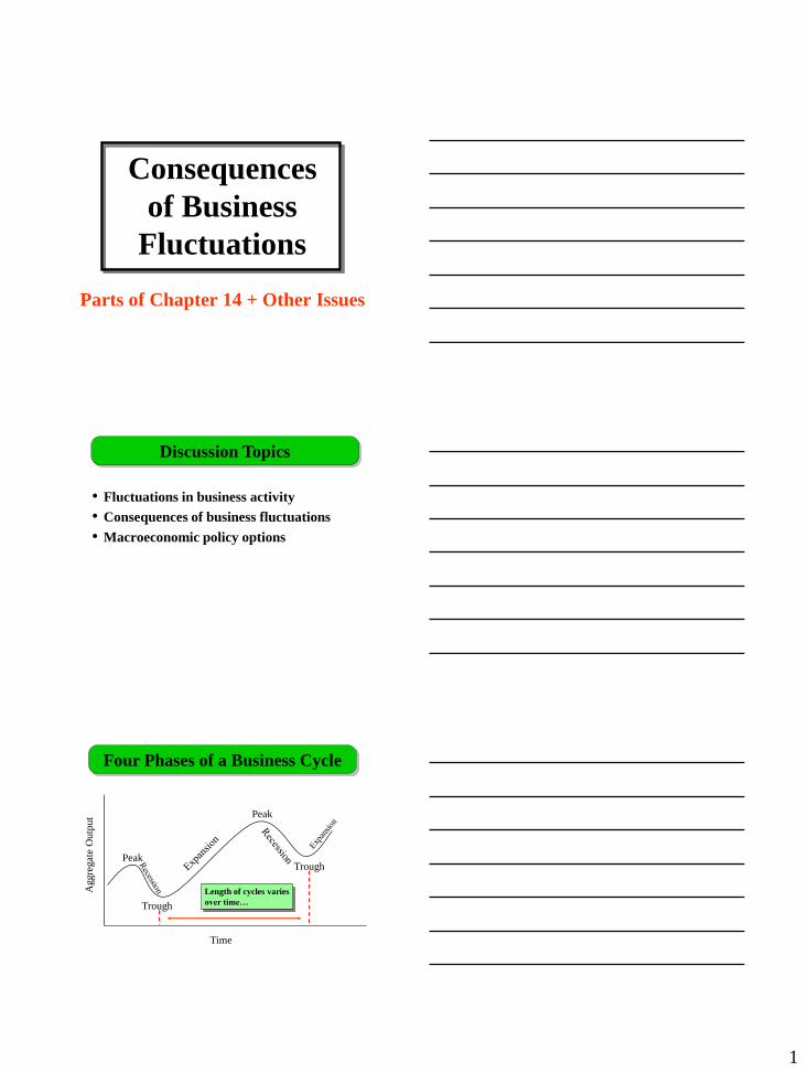
Length of cycles varies
over time…
Four Phases of a Business Cycle
Aggre
gat
e O
utp
ut
Time
Peak
Trough
Peak
Trough

2
• Keynesian – equilibrium levels differ from full
employment - changes to get to full employment
gives rise to the cycles
• Exogenous shocks – wars, credit crunch etc.
• Technological shocks - lumpy changes that increase
productivity
• Political – elect different administrations with
different policy goals
Causes of Business Cycles
• Lagging indicators - business inventories, duration
of employment, average interest rate
• Coincident indicators - current production, current
disposable income, current sales
• Leading indicators - new orders for goods, new
building permits, new investment in plant and
equipment, changes in the money supply
– Forecasting models - mathematical methods of
forecasting future trends in the economy
Indicators of Economic Activity
Conference Board – Components 2009 Weight /
Factor
Average weekly hours, manufacturing 0.2549
Average weekly claims, unemployment insurance 0.0307
Manufacturers’ new orders, consumer goods and materials 0.0774
Index of supplier deliveries – vendor performance 0.0677
Building permits, new private housing units 0.0270
Stock prices, 500 common stocks 0.0390
Money Supply, M2 0.3580
Interest rate spread, 10-year treasury bonds less federal funds 0.0991
Index of consumer expectations 0.0282
Manufacturers’ new orders, non-defense capital goods 0.0180
Leading Economic Indicators
http://www.conference-board.org/pdf_free/economics/bci/flaky.pdf
3
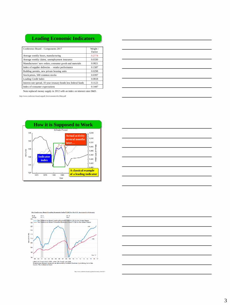
Conference Board – Components 2017 Weight /
Factor
Average weekly hours, manufacturing 0.2774
Average weekly claims, unemployment insurance 0.0330
Manufacturers’ new orders, consumer goods and materials 0.0821
Index of supplier deliveries – vendor performance 0.1587
Building permits, new private housing units 0.0298
Stock prices, 500 common stocks 0.0397
Leading Credit Index 0.0818
Interest rate spread, 10-year treasury bonds less federal funds 0.1123
Index of consumer expectations 0.1447
Leading Economic Indicators
http://www.conference-board.org/pdf_free/economics/bci/flaky.pdf
Note replaced money supply in 2012 with an index on interest rates S&D.
Indicator
index
Actual activity
several months
later…
A classical example
of a leading indicator
How it is Supposed to Work
http://www.conference-board.org/data/bcicountry.cfm?cid=1

4
http://www.conference-board.org/data/bcicountry.cfm?cid=1
Most Recent Notice Downturn Sept.
• Fluctuations in the unemployment rate
(civilian and capital) and implications for
policy
• Fluctuations in the rate of inflation and
implications for policy
Consequences of Business
Fluctuations
Monthly Unemployment Jan. 1948
– October 2017
Unemployment rate
during the great
depression was 25%
Full employment
barometer?

5
Monthly Unemployment U.S., Texas,
and B/CS 1976 – Sept. 2015
Texas lagged at the
start of the recession
Texas lagging at the
recovery?
Rate Number of civilians unemployed
Size of total civilian labor force =
where the size of the total civilian labor force is
determined by subtracting those not seeking jobs
(homemakers, students, etc.) from the total non-
institutional population (those not in prison) over
16 years of age, as well as, those who are in military
service.
Calculation of Civilian
Unemployment Rate
Assume the following values
Civilian labor force1 153.975 million
Employed persons 138.275 million
Unemployment 15.700 million
Not in force 82.316 million
Rate 15.700
153.975
=
= .102 or10.2 percent
1 The civilian labor force equals total population minus those not
seeking employment over age 16, those in institutions, and the military.
Example Oct. 2009
http://www.bls.gov/news.release/empsit.nr0.htm

6
Unemployment Rates
October
2009
March
2011
March
2013
March
2015
March
2017 Oct. 2071
All Workers
16+ 9 9.2 7.6 5.6 4.6 3.9
Adult men 7.3 10.2 8 6 4.9 3.9
Adult
women 7.3 8 7.2 5.1 4.1 3.8
Teenagers
16-19 21.5 23.6 23.3 17 13.1 13.4
White 8.5 5.3 6.9 4.9 4 3.3
Black /
African
American 13.5 15.5 12.8 10 9.1 7.5
Hispanic or
Latino 12.2 11.9 9.5 7 5.2 4.6
Earnings
Seasonally
adjusted
Private Workers Oct-09 Mar-11 Mar-13 Mar-15 Mar-17 Oct.-17
Average hours of
work /week 33.8 34.3 34.5 34.5 34.3 34.4
Average hourly
earnings 22.06 22.87 23.8 24.85 26.13 26.53
Average weekly
earnings 745.63 784.44 821.1 857.33 896.26 912.63
• Frictional - changing jobs and currently unemployed
• Cyclical - associated with business cycles
• Seasonal - associated with seasonal business activity
• Structural - associated with technological change
Forms of Unemployment

7
Monthly U.S. Percent Utilization of Refinery
Operable Capacity Jan. 1985 – Aug. 2017
Hurricane Ike
Hurricane Rita
Decreased from 92 to 81
Dec 2013 – Feb. 2013
Currently at 92.8
• Sustained rise in the general price level
• Not a change in the price of a single commodity
• Core rate of inflation excludes fuel and food price
increases
• Deflation (prices falling) vs. disinflation (prices
increasing at a slower rate)
What is Inflation?
CPI Index
• Consumer Price Index (CPI)
– CPI - represents changes in prices of all goods and
services purchased for consumption by urban
households
– Weighted basket of goods – Food and beverages, housing, apparel,
transportation, medical care, recreation, education and communication, and other goods
and services http://www.bls.gov/cpi/

8
Food and Beverages 14.649
Housing 42.634
Apparel 3.034
Transportation 15.318
Medical Care 8.539
Recreation 5.663
Education and communication 6.984
Other Goods and Services 3.178
Components / Weights in CPI 2016
https://www.bls.gov/cpi/cpiri_2016.pdf
Example Sub Category Weights
The consumer price index is a weighted average of
the prices consumers pay for goods and services.
It is measured by:
CPI =
Cost current year
Cost = WFB(PFB) + WH(PH) + … + WOTHER(POTHER)
= 15.757(PFB) + 43.421(PH) + … + 3.386(POTHER)
Cost of market basket in current year
Cost of market basket in base year × 100
Weights
Measuring the CPI

9
Grade Calculations
A) Total points = 600 possible = HW + clicker + tests + final + bonus points
B) HW 175 points = (sum of HW points / 429) * 175 = number out of 175
Note the value of 429 includes all possible HW
C) Clicker points = 75 possible = (sum of clicker points / 95.75)*75 - based
on values up to the start of class today will change as we have more
clicker questions
D) Test points = 200 possible = two highest test scores
E) Final 150 points – CURRENTLY YOU HAVE ZERO POINTS
F) Bonus points – added to total points = 10 possible = 5 each for out of class
videos
G) Up to you to check for missing / problems with grades by Friday
e-mail: [email protected]
A) We reserve the right to correct errors
The rate of inflation can be measured by the percent
change in the CPI, or
Inflation rate = current CPI – previous CPI
previous CPI
If the CPI was 216.17 in the last half of 2008 and
213.139 in the first half of 2009 what was the rate
of inflation rate
= (213.139 – 216.177) ÷ 216.1779
= -0.014 or -1.4%
Calculating Rates of Inflation
Year CPI Inflation rate
2005 195.300 ---
2006 201.600 = (201.6 – 195.3) / 195.3
= 0.0323 = 3.23%
2007 207.342 = (207.342 - 201.600) / 201.600
= 0.0285 = 2.85%
2008 215.303 =(215.303 – 207.342) / 207.342
= 0.0384 = 3.84%
Calculating Rates of Inflation

10
Annual Rates 1913 - 2016
Inflation thought
to be “under
control” in this
range. FED
2012 long run
goal is 2% Brought about a major
monetary policy action
CPI and Core Index –Quarterly
Red line – core some differences – mainly less variability
When describing growth in the economy on
the nightly newscast, the newscaster will
refer to the growth in real GDP after adjustments
for inflation. In the above example, real GDP
grew over the 1992-1999 period, but not at the
rate implied by comparisons in nominal terms.

11
GDP nominal rate of increase = (86-60)/60 *100 = 43%
GDP real rate of increase = (69-60)/60 *100 = 15%
Difference is because of inflation and not an increase in
productivity
Nominal and Real Growth GDP
Annual 1929 - 2016
• New Zealand Economist
– Educated at London School of Economics
– Phillips curve and MONIAC
• Early career
– Crocodile hunter and cinema manager
– Studied electrical engineering before the war
• WWII
– Singapore and than Java
– Captured
• learned Chinese, repaired and miniaturized a secret radio,
fashioned a secret water boiler for tea which hooked into camp
lighting system
W.E. Phillips

12
Phillips Curve U
nem
plo
ym
ent R
ate
Inflation Rate
9%
4%
3% 6%
Phillips curve named after
British economist A. W.
Phillips…
Policies that reduce
unemployment may
increase inflation in
the short run, and
vice versa…
Demand Pull Inflation
Pric
e L
ev
el
Y0 YPOT
AD0
AS
YFE
P0
AD1
P1
Y1
Inflation rate
(P1 – P0) ÷ P0
Aggregate Output
Demand oriented policies
that shift the aggregate
demand curve from AD0
to AD1 “pull up” the
general price level from P0
to P1.
This small increase in
inflation may make sense
since output increased
from Y0 to Y1, which would
lower unemployment.
Demand Pull Inflation and Unemployment
Pric
e L
ev
el
Y0 YPOT
AD0
AS
YFE
P0
AD1
P1
Y1 Inflationary gap
Created YE =
YPOT > YFE Inflation rate
(P3 – P1) ÷ P1
AD3
P3
Aggregate Output
Demand oriented policies
to maximize output at the
economy’s potential or
YPOT may bring about a
substantial increase in the
general price level (and
hence rate of inflation) for
a relatively small gain in
output and employment.

13
Cost Push Inflation and Unemployment
Pric
e L
evel
Y0
AS0
P0
AD0
P
1
Y1
Inflation rate
(P1 – P0) ÷ P0
Aggregate Output
Increase in the cost of
production thus a decrease is
AS0 to AS1 may bring about an
increase in the general price
level (and hence rate of
inflation) and a decrease in
output and employment.
AS1
Supply Side – Normal Range
Pric
e L
ev
el
Y0
AD0
AS0
YFE
P0
P1
Y1
Inflation rate
(P1 – P0) ÷ P0 Aggregate Output
AS1 Supply oriented policies that
enhance productivity reduce
the general price level.
Policies – See production
Research / Development
Technology
Infrastructure
Subsidies
Tax rates on business
Stimulates Y as with
demand side policies
Demand vs. Supply Policies
Pric
e L
ev
el
Y0
AD0
AS0
YFE
P0
P1
Y1
Aggregate Output
AS1
Pric
e L
ev
el
Y0
AD0
AS0
YFE
P0
P1
Y1
Aggregate Output
AD1
Both demand and supply
oriented policies stimulate
aggregate output.
Demand expansion policy “pulls up” the general price level….
Supply expansion policy reduces the general price level …

14
Demand vs. Supply Policies
YFE - new
AS1
Pric
e L
evel
Y0
AD0
AS0
YFE
P0
P1
Y1
Aggregate Output
AD1
In reality, both forms of
policy are typically carried
out at the same time.
New Equilibrium
Change in price levels depends
on the shifts in the two curves
New YFE
Summary
• A business cycle has four phases: peak, recession,
trough and expansion
• The two major consequences of business fluctuations
are unemployment and inflation
• Know how to calculate the civilian unemployment
rate and the rate of inflation facing consumers
• Understand the nature of the index of leading
economic indicators
• Understand the concept graphing of demand pull
inflation
• Understand the Phillips curve and demand and
supply policy impacts


![[PPT]Farm Management - Department of Agricultural …agecon2.tamu.edu/people/faculty/conner-richard/Notes/... · Web viewFarm Management Chapter 2 Management and Decision Making Chapter](https://img.pdfslide.us/doc/110x75/5aab8f1a7f8b9a8d678bf332/pptfarm-management-department-of-agricultural-viewfarm-management-chapter.jpg)