Connectivity properties of a random radio network

J. Ni, M S c , MlEE S.A.G. Chandler, PhD, MlEE

Indexing terms: Connectivity properties, Random radio network

I I Abstract: Pure and routing-algorithm-based con- nectivities of random radio networks are studied by theoretical analyses and computer simulation respectively. The ‘magic number’ of average neigh- bours of each station from connectivity point of view is obtained.

1 Introduction

One of the key issues in radio communication network design is to find the adequate number of neighbours for each station so that certain network performance can be achieved. For a network with certain station density, increasing the average number of neighbours by increas- ing transmission range can improve its performance parameters such as throughput, connectivity and trans- mission delay etc., whereas increasing transmission range to achieve this will, on the other hand, lead to larger transmitting power requirement and higher collision probability as well. Hence, the optimal point is a com- promise.

A number of papers concerning with this problem can be found in literature [1-9, 17-19]. It is well known that finding the adequate number of neighbours is a ‘hard-to- solve’ multiparameter optimisation problem. However, if the stress of consideration is put on a specific parameter, which varies with different demands, the problem becomes tractable.

In packet radio networks with information being transmitted in packetted data over shared channels, network, throughput is the most important parameter and therefore the main consideration. The authors of Ref- erences 1 and 2 studied the optimal transmission range problem of slotted ALOHA packet radio networks from this point of view. They found that the optimal number of neighbours, which is sometimes called the ‘magic number’, is in the range 6 to 8.

In another type of network such as a distributed radio network for rural telephony [16], connectivity is of top importance. Then, what is the relationship between network connectivity and average number of neighbours of each station? The results of Reference 3, showed that, if the average number of neighbours of each station is a constant, then for sufficiently large area, the network will almost certainly be disconnected. This implies that from a network connectivity point of view, no ‘magic number’ could ensure a random network over sufficiently large area being fully connected. However, this does not mean

0 IEE, 1994 Paper 11971 (E8), first received 15th July 1993 and in revised form 23rd February 1994 The authors are with the Department of Engineering, University of Warwick, Coventry CV4 7AL, United Kingdom

I E E Proc.-Commun., Vol. 141, No. 4, August 1994

that the ‘magic number’ is useless. Gilbert [6] had shown that there is a critical number N o , such that if the average number of neighbours is larger than N o , the random plane network contains an infinite connected component with nonzero probability. The most recent result for No is that 2.195 < No < 10.526 [3].

In practical situations, networks with finite number of stations are usually limited in a certain area, and it is evident that the probability of connection over a given distance will increase with density. In Reference 4, the probability of being able to make connection between stations as the function of distance between them and station density was studied theoretically. It was found that the ‘magic number’ is about 5.

In this paper, connectivity properties of random radio networks as a function of network features, such as average number of neighbours and so on, will be studied. By definition, network connectivity is the average prob- ability of being able to make connection between any station pairs over the whole network. More precisely speaking, it has the following two-fold meaning:

pure connectivity (P-connectivity), which characterizes the inherent connecting property of the random network; and routing algorithm based connectivity (RAB-connect- ivity), which represents the actually achievable con- necting property of random networks employing a specific routing algorithm.

Theoretical analyses and simulation are carried out for both the above two parameters. Comparison between RAB-connectivity and P-connectivity, RAB- connectivities of the same network employing different routing algorithms are presented.

2 Network model and definitions

The network considered in the following sections is mod- elled as a two dimensional Poisson point process with density being A stations/square units and within an area of the size of A square units, i.e.

(1A)’e- ’* {finding i stations in an area of size of A } = ~

i !

(1) The transmitting radii of all the stations are a units. Then, it is expected that there are

Q = na2A (2)

The authors would like to thank Mr. S. Braith- waite of Southampton University and Professor D.J. Whitehouse for their helpful discussion.

289

other stations on average within any one station’s radio range except those at the edge of the network. These Q stations are called the neighbours of the station. The expected total number of stations in the network is

N = AA (3) The rigorous definitions of the two-fold meaning of network connectivity are

Definition I : The pure-connectivity (P-connectivity) of a random network, with transmitting radii of all the sta- tions being identical and of certain value, is defined as the average probability of being able to make connection between an arbitrary station pair in the network.

DeJinition 2: The routing algorithm based connectivity (RAB-connectivity) of a random network is defined as the average probability of being able to make connection between an arbitrary station pair by employing a specific routing algorithm.

P-connectivity is the inherent connecting property of a random network and therefore independent of the proto- cols employed in it. So long as the network is fully con- nected in terms of graph theory, its P-connectivity will be 1. RAB-connectivity is the actually achievable network connectivity by employing a specific routing algorithm. It is quite different for different routing algorithms and represents the efficiency of the routing algorithm in finding existing routes.

3 P-connectivity of random network

3.1 Theoretical analyses Theoretical analysis of the P-connectivity of a random network can be carried out in several ways. Although the most direct way is concerned with coverage processes [lo], the undetermined distributions of many important random variables make the problem almost numerically unsolvable. An approximate but relatively simple analysis is described as follows

(a) Find out the probability distribution of the distance between an arbitrary station pair in the network.

(b) Find out the probability distribution of being able to make connection with another station at given dis- tance.

(c) Calculate the average probability of being able to make connection between station pairs.

3.1.1 Distribution of distance between station pairs: As is assumed in Section 2, stations are uniformly distrib- uted in an area (represented by d) of size of A (see Fig. 1). Put area d in a reference Cartesian coordinates C,, then a station’s location (s,, y,) in C , is a two- dimensional random variable with joint probability density being

(4)

Arbitrarily choosing one station’s position in C , , say (st, y , ) , as the centre of a second reference Cartesian coordi- nates C, , then position of stations in C, , (x, , y,), has the same joint probability density as above, i.e.

1 fc&, 1 Y 2 ) = 1 (5)

290

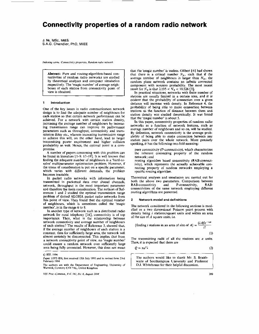
The distance between a station at (x,, y,) and the given station (located at (0,O) in C, or (x,, y,) in C,) is

(6) r = JC.: + Y 9

Fig. 1 Network area and two reference Cartesian coordinates

To find the probability distribution of r, it is convenient to use polar coordinates. The relationship between (x2, y 2 ) and ( I , 0) are

x, = r cos 0 y, = r sin 0

(7)

(8) The joint probability density of (r, 0) is then

fR. e(r> = f (9)

and the probability density of r is

where, 4 is the accumulated angle along the circle of radius r centred at (x,, y,) in C, covering the area d. In Fig. 1, for example, 4 = 4, + 4,. This is the probability density of the distance between an arbitrary station and the given station located at (x,, y , ) in C , .

Changing the centre of reference coordinates C, to a different station’s position, the probability density of the distance between an arbitrary station and another given station can be found in the same way. Therefore, the probability density of the distance between an arbitrary station pair is the expected value off(r) over the whole area d in C,, that is

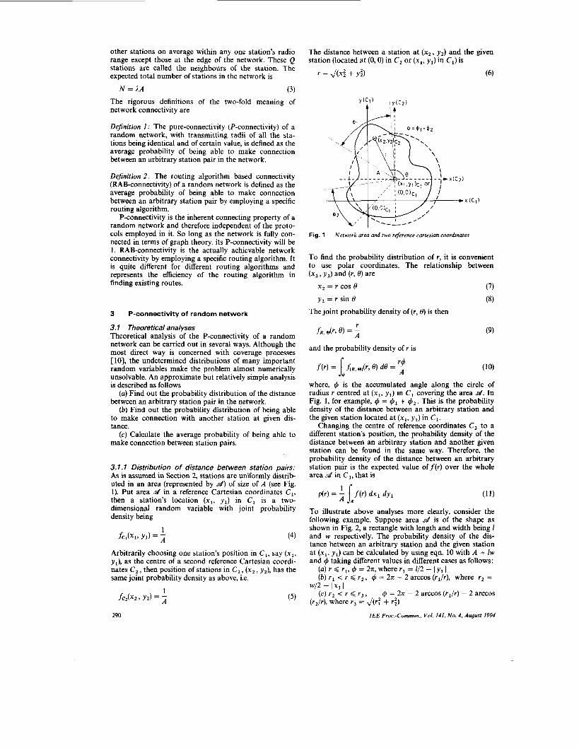
To illustrate above analyses more clearly, consider the following example. Suppose area d is of the shape as shown in Fig. 2, a rectangle with length and width being 1 and w respectively. The probability density of the dis- tance between an arbitrary station and the given station at (x,, y,) can be calculated by using eqn. 10 with A = lw and 4 taking different values in different cases as follows:

(a) r < r , , 4 = 2n, where r , = 1/2 - I y , I (b) r 1 < r < r z , 4 = 2x - 2 arccos ( r l / r ) , where r , =

(c) r , < r < r 3 , 4 2 - I x1 I

4 = 2n - 2 arccos ( r l / r ) - 2 arccos (r,/r), where r3 = ,,/(rf + r;)

I E E Proc.-Commun., Vol. 141, No. 4 , August 1994

(4 r3 < r < r4, q5 = 4 2 + arcsin (rl/r) + arcsin (r2/r), where r4 = w - rz

(e) r, < r < r5, q5 = n/2 + arcsin (rl/r) + arcsin (rz/r) - 2 arccos (rdr), where r5 = J(r: + r i ) (f) r5 < r < r6, q5 = 4 2 + arcsin (rl/r) - arccos (r4/r),

where r6 = 1 - r1 (9) r6 < r < r7 , q5 = 4 2 + arcsin (r2/r) - arccos (r4/r)

- 2 arccos (r6/r), where r , = J(rg + r:) (h) r7 < r < rg , q5 = n/2 - arccos (r4/r) - arccos (r6/r),

where r8 = J(r: + r:) (i) r > r8 , q5 = 0

Fig. 2 A typical area .d with stations uniformly distributed in it

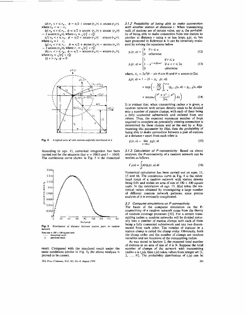
According to eqn. 11, numerical integration has been carried out for the situation that w = 100.0 and I = 100.0. The continuous curve shown in Fig. 3 is the numerical

0.016r 0.0141

> 0.012-

: 0.01 -

- cn

v g 0.008 - n

2 n 0006-

0004 -

0.002

0 0 20 40 60 80 I00 120 I40 I60

distance

Fig. 3 Distribution of distance between stution pairs in random network Ana size = 100 x I00 square units ~ theoretical result

0 simulated result

result. Compared with the simulated result under the same conditions (circles in Fig. 3), the above analyses is proved to be correct.

IEE Proc.-Commun., Vol. 141, No. 4 , August 1994

3.1.2 Probability of being able to make connection with another station at distance r: When transmitting radii of stations are of certain value, say a, the probabil- ity of being able to make connection from one station to another at distance r using n or less hops, pn(r, a), has been presented in Reference 4. It can be iteratively evalu- ated by solving the equations below

1 i f r < a = 0 otherwise

i f r < a p2(rr a) = I - e-AlQ'n42 if a < r < 2a (13) 1: otherwise

where, A, = 2a2(0 - sin 0 cos 0) and 0 = arccos (r/2a).

p k , a) = 1 - (1 - P,- a))

x arccos( r2 + xz - a2

2rx ) dx)

It is evident that, when transmitting radius a is given, a random network with certain density tends to be divided into a number of station clumps, with each of them being a fully connected subnetwork and isolated from any others. Thus, the expected maximum number of hops required to complete an potentially existing connection is determined by these clumps and at the end by a. Rep- resenting this parameter by H(a), then the probability of being able to make connection between a pair of stations at a distance r apart from each other is

3.1.3 Calculation of P-connectivity: Based on above analyses, the P-connectivity of a random network can be written as follows

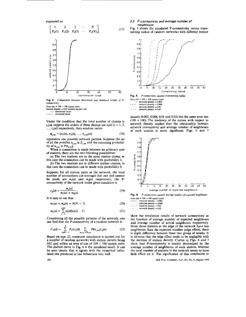
C p ( 4 = A~)P&, a) dr (16) J: Numerical calculation has been carried out on eqns. 11, 15 and 16. The continuous curve in Fig. 4 is the calcu- lated result of a random network with station density being 0.01 and within an area of size of 100 x 100 square units. In the calculation of eqn. 15, H(a) takes the sta- tistical values obtained by investigating a large number of different random network patterns, since precise analysis of it is extremely complicated.

3.2 Computer simulations on P-connectivity The bases of the computer simulation on the P- connectivity of a random network come from the theory of random coverage processes [lo]. For a certain trans- mitting radius a, random networks will be divided natur- ally into a number of station clumps with each of them being a fully connected subnetwork and any two discon- nected from each other. The number of stations in a station clump is called the clump order. Obviously, both the clump order and the number of clumps are random variables and are functions of the transmitting radius.

As was stated in Section 2, the expected total number of stations in an area of size of A is N . Suppose the total number of clumps of the network with transmitting radius a is [,(a), then [,(a) takes values from integer set { 1, 2, . . . , N}. The probability distribution of &(a) can be

291

expressed as

lr J 0.9

0.8

0.6

f 0-3

0-2

0 IO 20 30 LO 50 60 Ironsmisston range

Fig. 4 connectivity Area size = 100 x I00 square units Station density = 0.01 stationslsquare unit __ thwretical result ~ _ _ _ simulated result

Comparison between theoretical and simulated results of P-

Under the condition that the total number of clumps is t,(a), suppose the orders of these clumps are nia) (i = 1, 2, . . . , [,(a)) respectively, then random vector

nre(o) (nl(a), nda), . . ' 1 nrda) ) (18) represents one possible network pattern. Suppose the set of all the possible n,(,, is Sir(,,) and the occurring probabil-

When a connection is made between an arbitrary pair of stations, there are the two following possibilities:

(a) The two stations are in the same station clump, in this case the connection can be made with probability 1.

(b) The two stations are in different station clumps, in this case the connection can be made with probability 0.

Suppose, for all station pairs in the network, the total number of connections (on average) that can and cannot be made are m,(a) and mka) respectively, the P- connectivity of the network under given condition is

ity of nrc(o) is P(nrC(a$

(17)

3.3 P-connectivity and average number of neighbours

Fig. 5 shows the simulated P-connectivity versus trans- mitting radius of random networks with different station

Considering all the possible patterns of the network, one can find that the P-connectivity of a random network is

N

CAa) = 1 PAt,(a)) 1 P(nrc(a))cp(a) (22) r,C) = I "Qbl E .%<a)

Based on eqn. 22, computer simulation is carried out for a number of random networks with station density being 0.01 and within an area of size of 100 x 100 square units. The dashed curve in Fig. 4 is the simulated result. It can be seen clearly that it agrees with the numerical calcu- lated one presented in last subsection very well.

292

transmitting radius

P-connectivity against transmitting radius Fig. 5 Area size = 100 x 100 square units __ network density = 0.002 ~~~- network density = 0.W

. . . . . . . network density = 0.01 network density = 0.03

density (0.002,0.006,0.01 and 0.03) but the same area size (100 x 100). The tendency of the curves with respect to network density implies that the relationship between network connectivity and average number of neighbours of each station is more significant. Figs. 6 and 7

average number of expected neighbours

Fig. 6 Area size = LOO x I00 square units ~ network density = 0.002

network density = 0.006 network density = 0.01 network density = 0.03

P-connectivity against average number of expected neighbours

_ _ _ _ . . . . . . .

show the simulation results of network connectivity as the function of average number of expected neighbours and average number of actual neighbours respectively. Since those stations at the edge of the network have less neighbours than the expected number (edge effect), there is slight difference between these two group of results. It is obvious that the edge effect tends to be negligible with the increase of station density. Curves in Figs. 6 and 7 show that P-connectivity is mainly determined by the average number of neighbours of each station, whereas the total number of stations in the network seems to have little effect on it. The significance of this conclusion in

I E E Proc.-Commun., Vol. 141, No. 4 , August I994

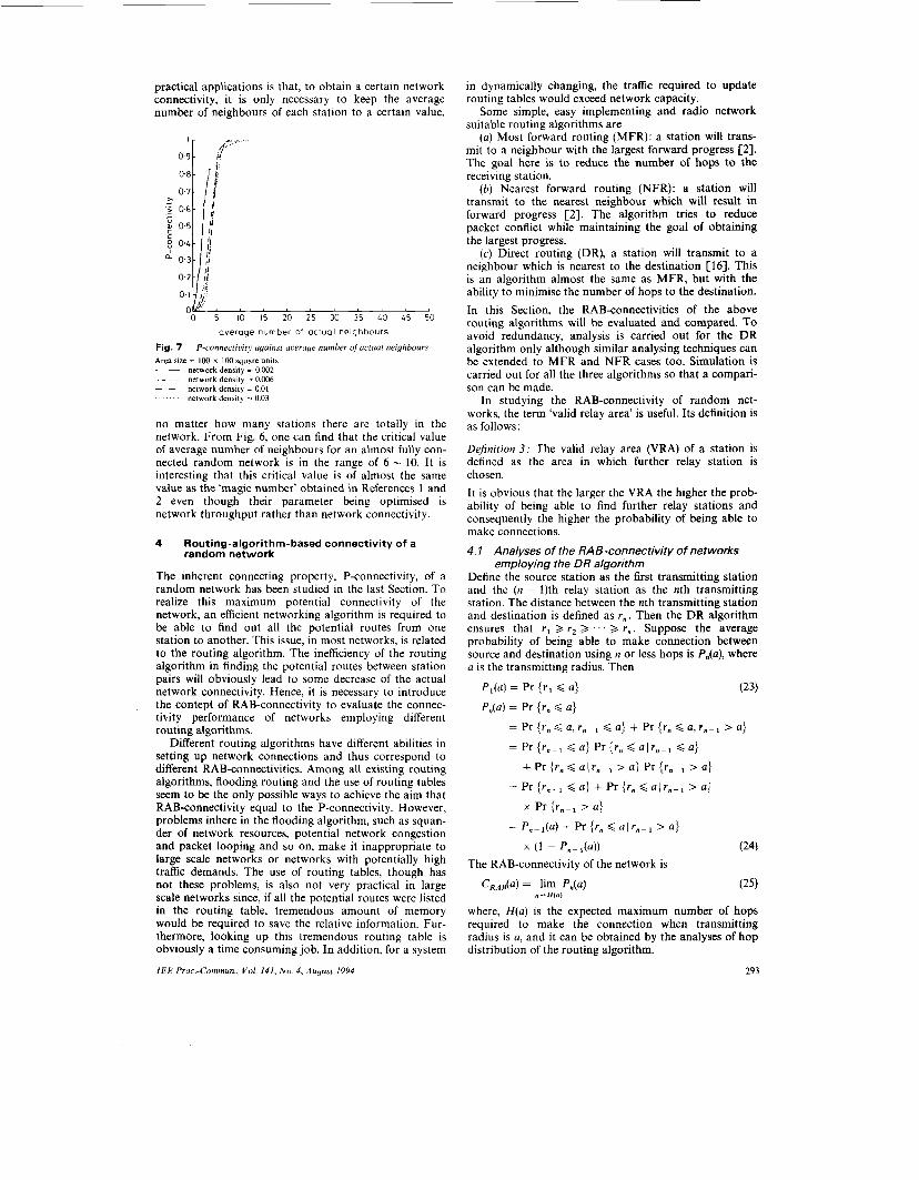
practical applications is that, to obtain a certain network connectivity, it is only necessary to keep the average number of neighbours of each station to a certain value,

O i [ {--

0 .. , , , , , , , , , , 0 5 10 15 20 25 30 35 40 45 50

overoqe number of octual neighbours

Fig. 7 Area size = 100 x 1M square units __ network density = 0.002 _ _ ~ ~ network density = 0.006

. . . . . . .

P-connectivity against average number of actual neighbours

network density = 0.01 network density = 0.03

no matter how many stations there are totally in the network. From Fig. 6, one can find that the critical value of average number of neighbours for an almost fully con- nected random network is in the range of 6 - 10. I t is interesting that this critical value is of almost the same value as the 'magic number' obtained in References 1 and 2 even though their parameter being optimised is network throughput rather than network connectivity.

4 Routing-algorithm-based connectivity of a

The inherent connecting property. P-connectivity, of a random network has been studied in the last Section. To realize this maximum potential connectivity of the network, an efficient networking algorithm is required to be able to find out all the potential routes from one station to another. This issue, in most networks, is related to the routing algorithm. The inefficiency of the routing algorithm in finding the potential routes between station pairs will obviously lead to some decrease of the actual network Connectivity. Hence, it is necessary to introduce the contept of RAB-connectivity to evaluate the connec- tivity performance of networks employing different routing algorithms.

Different routing algorithms have different abilities in setting up network connections and thus correspond to different RAB-connectivities. Among all existing routing algorithms, flooding routing and the use of routing tables seem to be the only possible ways to achieve the aim that RAB-connectivity equal to the P-connectivity. However, problems inhere in the flooding algorithm, such as squan- der of network resources, potential network congestion and packet looping and so on, make it inappropriate to large scale networks or networks with potentially high traffic demands. The use of routing tables, though has not these problems, is also not very practical in large scale networks since, if all the potential routes were listed in the routing table, tremendous amount of memory would be required to save the relative information. Fur- thermore, looking up this tremendous routing table is obviously a time consuming job. In addition, for a system

random network

I E E Proc.-Commun., Vol. 141, N o . 4 , August 1994

in dynamically changing, the traffic required to update routing tables would exceed network capacity.

Some simple, easy implementing and radio network suitable routing algorithms are

(a) Most forward routing (MFR): a station will trans- mit to a neighbour with the largest forward progress [Z]. The goal here is to reduce the number of hops to the receiving station.

(b) Nearest forward routing (NFR): a station will transmit to the nearest neighbour which will result in forward progress [Z]. The algorithm tries to reduce packet conflict while maintaining the goal of obtaining the largest progress.

(c) Direct routing (DR), a station will transmit to a neighbour which is nearest to the destination [16]. This is an algorithm almost the same as MFR, but with the ability to minimise the number of hops to the destination. In this Section, the RAB-connectivities of the above routing algorithms will be evaluated and compared. To avoid redundancy, analysis is carried out for the DR algorithm only although similar analysing techniques can be extended to MFR and NFR cases too. Simulation is carried out for all the three algorithms so that a compari- son can be made.

In studying the RAB-connectivity of random net- works, the term 'valid relay area' is useful. Its definition is as follows:

Dejinirion 3 : The valid relay area (VRA) of a station is defined as the area in which further relay station is chosen. It is obvious that the larger the VRA the higher the prob- ability of being able to find further relay stations and consequently the higher the probability of being able to make connections. 4.1 Analyses of the RAE-connectivity of networks

employing the DR algorithm Define the source station as the first transmitting station and the (n - 1)th relay station as the nth transmitting station. The distance between the nth transmitting station and destination is defined as rn . Then the DR algorithm ensures that r1 > r2 3 . . > rn. Suppose the average probability of being able to make connection between source and destination using n or less hops is P&), where a is the transmitting radius. Then

Pl(a) = Pr {rl < a } (23) P,(a) = Pr {r, < a)

= Pr { rn<a , r , - , < a } + Pr {r, < a , r n - l > a )

= P r { r n - l < a } P r { r n < a l r " - l < a )

+ Pr {rn < alrn- l > U } Pr { r n - l > U }

= Pr { r n - t < a} + Pr {rn < ulrn-l > U }

x Pr {r,-, > a }

=P, - , ( a )+Pr{ r , ,<a l r , - , > a }

x (1 - P " - l ( 4 (24) The RAB-connectivity of the network is

C,,,,(u) = lim P.(a) "-€I@)

where, H ( a ) is the expected maximum number of hops required to make the connection when transmitting radius is a, and it can be obtained by the analyses of hop distribution of the routing algorithm.

293

Eqn. (23) can be solved by the integration of eqn. 11, i.e.

PI@) = d r , ) dr1 (26) l For all other n > 1 cases, if Pr {r , < a I r,- > a } is avail- able, Pn(a) can then be easily obtained. In order to solve this problem, define A, + B, as the intersection area of nth transmitting station's radio range and the round area with radius r, centred at the destination and A, as the intersection area of nth transmitting station's radio range and the round area centred at destination with radius being r,,,. Then (see Fig. 8) the VRA of nth transmitting

Fig. 8 Routing procedure oJdirert routing algorithm

station is B, + A, - ( E , + A,) n A ,

A,, = a28, + r;+ 140 - ar, sin 0, and

where,

0. = arccos

r; + r i+ , - a' 2r"r"+l

4" = arccos

A, + B, = a'@, + rimn - ar, sin 0, where,

0, = arccos (k) @" = x - 20,

According to the definition, A, is a part of the nth trans- mitting station's radio range in which the station intends but fails to find a further relay station (i.e. the ( n + I)th transmitting station). Hence, A, = 0 and therefore ( E , + A,) n A, = 0. Based on all of these

Pr {no station in A, & at least one in B , } Pr {at least one station in A , + B , }

- -

e - A A i ( l - e - A B ~ )

1 - , - i l A ~ + B i ) - - (33)

(34)

It is evident that the probability distribution of random variable rm is related to that of two others, r n - l and r m - z . One then has

(35) Pr { r , < R n l r n - l } = 1 - Pr { r , > R , l r , - l }

and

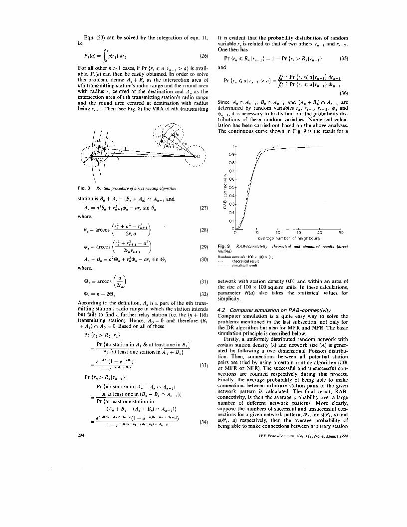
(36) Since A,nA,- , , B,nA,- , and (A,+B, )nA, - , are determined by random variables r , , r m - ,, r n - 2 , $J" and 4"- it is necessary to firstly find out the probability dis- tributions of these random variables. Numerical calcu- lation has been carried out based on the above analyses. The continuous curve shown in Fig. 9 is the result for a

0.8 O'gt 0.7 i'

0.11 d' OW 0 10 20 30 40 50

average number of neighbours

Fig. 9 RAB-connectivity : theoretical and simulated results (direct routing) Random network: IW x 100 Y 0.1

theoretical result simulated result ~~~~

network with station density 0.01 and within an area of the size of 100 x 100 square units. In these calculations, parameter H(a) also takes the statistical values for simplicity.

4.2 Computer simulation on RAE-connectivity Computer simulation is a quite easy way to solve the problems mentioned in the last subsection, not only for the DR algorithm but also for MFR and NFR. The basic simulation principle is described below.

Firstly, a uniformly distributed random network with certain station density (A) and network size (A) is gener- ated by following a two dimensional Poisson distribu- tion. Then, connections between all potential station pairs are tried by using a certain routing algorithm (DR or MFR or NFR). The successful and unsuccessful con- nections are counted respectively during this process. Finally, the average probability of being able to make connections between arbitrary station pairs of the given network pattern is calculated. The final result, RAB- connectivity, is then the average probability over a large number of different network patterns. More clearly, suppose the numbers of successful and unsuccessful con- nections for a given network pattern, Pi, are $Pi, a) and u ( Y i , a ) respectively, then the average probability of being able to make connections between arbitrary station

IEE Proc.-Commun., Vol. 141, No. 4, August 1994 294

pairs in this network pattern is

% 0 7 -

2 0 6 -

(37)

;/ I / ,,

ok@ ~ , , , , , , , , , 0 5 I O 15 20 25 30 35 4 0 L5 50

average number of expected nelghbours

a 0 2 -

0 1 -

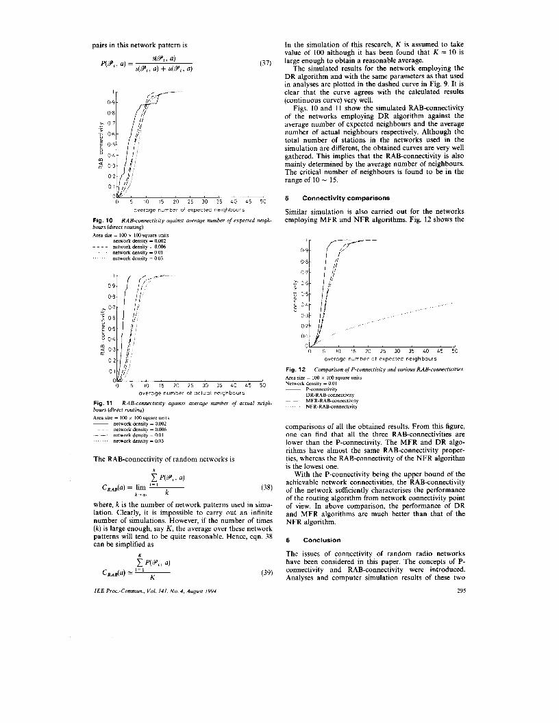
Fig. 10 bows (direct routing) Area size = 1 0 0 x I00 square units ~ network density = 0.002 ~-~~ network density = 0.006

RAE-connectivity against average number of expected

network density = 0.01 network density = 0.03 . . . . . . .

/I I/

/I /,

0 1 ' ' ' ' ' ' ' ' ' '

neigh-

averoge number of actual neighbours

Fig. 11 bours (direct routing) Area size = I00 x 100 square units

~ network density = 0.002 ~ _ _ _ network density = 0.006

RAB-connectivity against average number of actual neigh-

network density = 0.01 network density = 0.03 . . . . . . .

The RAB-connectivity of random networks is I

where, k is the number of network patterns used in simu- lation. Clearly, it is impossible to carry out an infinite number of simulations. However, if the number of times ( k ) is large enough, say K , the average over these network patterns will tend to be quite reasonable. Hence, eqn. 38 can be simplified as

K c PVi? a)

K CR,,(a) Y

IEE Proc.-Commun., Vol. 141, No. 4 , August 1994

(39)

In the simulation of this research, K is assumed to take value of 100 although it has been found that K = 10 is large enough to obtain a reasonable average.

The simulated results for the network employing the DR algorithm and with the same parameters as that used in analyses are plotted in the dashed curve in Fig. 9. It is clear that the curve agrees with the calculated results (continuous curve) very well.

Figs. 10 and 11 show the simulated RAB-connectivity of the networks employing DR algorithm against the average number of expected neighbours and the average number of actual neighbours respectively. Although the total number of stations in the networks used in the simulation are different, the obtained curves are very well gathered. This implies that the RAB-connectivity is also mainly determined by the average number of neighbours. The critical number of neighbours is found to be in the range of 10 - 15.

5 Connectivity comparisons

Similar simulation is also carried out for the networks employing MFR and NFR algorithms. Fig. 12 shows the

average number of expected neighbours

Fig. 12 Area size = 100 x 100 square units Network density = 0.01 ~ P-connectivity ~~~ ~ DR-RAB-connectivity

Comparison oJP-connectivity and various RAB-connectivities

MFR-RAE-connectivity . . . . . . . NFR-RAB-connectivity

comparisons of all the obtained results. From this figure, one can find that all the three RAB-connectivities are lower than the P-connectivity. The MFR and DR algo- rithms have almost the same RAB-connectivity proper- ties, whereas the RAB-connectivity of the NFR algorithm is the lowest one.

With the P-connectivity being the upper bound of the achievable network connectivities, the RAB-connectivity of the network sufficiently characterises the performance of the routing algorithm from network connectivity point of view. In above comparison, the performance of DR and MFR algorithms are much better than that of the NFR algorithm.

6 Conclusion

The issues of connectivity of random radio networks have been considered in this paper. The concepts of P- connectivity and RAB-connectivity were introduced. Analyses and computer simulation results of these two

295

parameters were presented. It was shown that, from con- nectivity point of view, the ‘magic number’ of the network is in the range of 6 - 10 for P-connectivity and 10 - 15 for the RAB-connectivity of the network employ- ing the DR algorithm. Comparison of different RAB- connectivity was also carried out. Based on the results obtained in this study, a connectivity criterion for mea- suring the performance of a routing algorithm was intro- duced.

7 References

1 TAKAGI, H., and KLEINROCK, L.: ‘Optimal transmission ranges for randomly distributed packet radio terminals’, IEEE Trans., 1984, COM-32, (3 ) , pp. 246-257

2 HOU, T.-C., and Li, O.K.: ‘Transmission range control in multihop packet radio networks’, IEEE Trans., 1986, COM-34, ( I ) , pp. 38-44

3 PHILIPS, T.K., PANWAR, S.S., and TANTAWI, A.N.: ‘Con- nectivity properties of a packet radio network model’, IEEE Trans., 1989, IT-35, (3, pp. 1044-1047

4 CHANDLER, S.A.G.: ‘Calculation of number of relay hops required in randomly located radio network’, Electron. Left.. 19x9, 25, (241, pp. 1669-1671

5 SHIAO, F.-M., and YEE, J.R.: ‘On determining the transmission range for multi-hop slotted ALOHA packet radio networks’. IEEE MILCOM’90, vol. 2, pp. 850-854

6 GILBERT, E.N.: ‘Random plane networks’, J . Soc. Indusf. Appl. Mofh., 1961,9, (41, pp. 533-543

7 PIRET, P.: ‘On the connectivity of radio networks’, IEEE Trans.. 1991, IT-37, (3, pp. 1490-1492

8 CHENG, Y.-C., and ROBERTAZZI, T.G.: ‘Critical connectivity phenomena in multihop radio models’, IEEE Trans., 1989. COM-37, (7), pp. 770-777

9 KLEINROCK. L., and SILVESTER, J.: ‘Optimum transmission radii for packet radio networks or why six is a magic number’. Conf. Rec. Nat. Telecommun. Conf. IEEE, Dec. 1978, pp. 4.3.1-4.3.5

I O HALL, P.: ‘Introduction to the theory of coverage processes’ (John Wiley & Sons, New York, 1988)

I I KENDALL, M.G.. and MORAN, P.A.P.: ‘Geometrical probability’ (Charles Grillin & C o . Ltd.. London, 1963)

12 MACK, C.: ‘The expected number of clumps when convex laminae are placed at random and with random orientation on a plane area’, Proc. Camh. Philos. Soc.. 1948, 50, pp. 581-585

13 MACK. C.: ’On clumps formed when convex lamminea or bodies are placed at random in two or three dimensions‘, Proc. Camh. Philos. Soc., 1950. 52, pp. 246-256

14 KELLERER. A.M.: ’On the number of clumps resulting from the overlap of randomly placed figures in a plane‘, J. Appl. Probab., 20, pp. 126-135

15 MILES, R.E.: ‘On the homogeneous planar poisson point process’, Math. Biosci., 1970, 6, pp. 85- 127

16 STEALEY, K.B.: ‘Protocols and control algorithms for dislributed radio telecommunications for rural areas’. MSC thesis, Department of Eneineering, University of Warwick. July 1992

17 NI, J., CHANDLER, S.A.G., and STEALEY. K.B.: ‘A distributed network radio system appropriate to rural telephony’. IEE Collo- quium on Radio systems for rural communications, January 1993, pp. 2-1-2-8

18 CHANDLER, S.A.G., BRAITHWAITE, S.J., and NI, J.. and STEALY. K.B.: ’A distributed rural telephone system for developing countries’. The 4th IEE Conference on Telecommunications, April 1993, pp. 193-198

19 CHANDLER, S.A.G.. NI, J., and BRAITHWAITE, SJ.: ‘Analysis and simulation of a distributed rural radiotelephone network’, 4th European Conference on Radio relay systems, Oct. 1993

296 IEE Proc.-Commun., Vol. 141. No. 4, Augusl 1994