Connected MeshesJohannes Unterguggenberger∗

StudentMartin IlcıkSupervisor

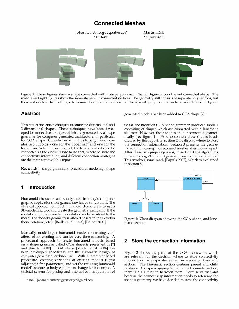
Figure 1: These figures show a shape connected with a shape grammar. The left figure shows the not connected shape. Themiddle and right figures show the same shape with connected vertices. The geometry still consists of separate polyhedrons, buttheir vertices have been changed to a connection-point’s coordinates. The separate polyhedrons can be seen at the middle figure.

Abstract

This report presents techniques to connect 2-dimensional and3-dimensional shapes. These techniques have been devel-oped to connect basic shapes which are generated by a shapegrammar for computer generated architecture, in particularfor CGA shape. Consider an arm: the shape grammar cre-ates two cuboids - one for the upper arm and one for thelower arm. When the arm is bent, the two cuboids should beconnected at the elbow. How to do that, where to store theconnectivity information, and different connection-strategiesare the main topics of this report.

Keywords: shape grammars, procedural modeling, shapeconnectivity

1 Introduction

Humanoid characters are widely used in today’s computergraphic applications like games, movies, or simulations. Theclassical approach to model humanoid characters is to use a3D-modelling tool and create the geometry manually. If themodel should be animated, a skeleton has to be added to themesh. The model’s geometry is altered based on the skeleton(bone rotations, etc.). [Badler et al. 1993], [Ratner 2003]

Manually modelling a humanoid model or creating vari-ations of an existing one can be very time-consuming. Aprocedural approach to create humanoid models basedon a shape grammar called CGA shape is presented in [?]and [Fiedler 2009]. CGA shape [Muller et al. 2006] hasbeen developed specifically for the automatic design ofcomputer-generated architecture. With a grammar-basedprocedure, creating variations of existing models is justadjusting a few parameters, and yet the resulting humanoidmodel’s stature or body weight has changed, for example. Askeletal system for posing and interactive manipulation of

∗e-mail: johannes.unterguggenberger@gmail.com

generated models has been added to GCA shape [?].

So far, the modified CGA shape grammar produced modelsconsisting of shapes which are connected with a kinematicskeleton. However, these shapes are not connected geomet-rically (see figure 1). How to connect these shapes is ad-dressed by this report. In section 2 we discuss where to storethe connection information. Section 3 presents the geome-try adaption concept to reconnect meshes after moved apart.After these two preparing steps, in section 4 the algorithmsfor connecting 2D and 3D geometry are explained in detail.This involves some math [Papula 2007], which is explainedin section 5.

Figure 2: Class diagram showing the CGA shape, and kine-matic section

2 Store the connection information

Figure 2 shows the parts of the CGA framework whichare relevant for the decision where to store connectivityinformation. A shape always has an associated kinematicsection. The kinematic section contains parent and childrelations. A shape is aggregated with one kinematic section,there is a 1:1 relation between them. Because of that andbecause the connectivity information needs to reference theshape’s geometry, we have decided to store the connectivity

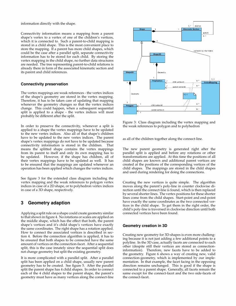
information directly with the shape.

Connectivity information means a mapping from a parentshape’s vertex to a vertex of one of the children’s vertices,which it is connected to. Such a parent-to-child mapping isstored in a child shape. This is the most convenient place tostore the mapping. If a parent has more child shapes, whichcould be the case after a parallel split, separate connectivityinformation has to be stored for each child. By storing thevertex mapping in the child shape, no further data structuresare needed. The tree representing parent-to-child relations isalready there in form of the associated kinematic section andits parent and child references.

Connectivity preservation

The vertex mappings are weak references - the vertex indicesof the shape’s geometry are stored in the vertex mapping.Therefore, it has to be taken care of updating that mappingwhenever the geometry changes so that the vertex indiceschange. This could happen, when a subsequent sequentialsplit is applied to a shape - the vertex indices will mostprobably be different after the split.

In order to preserve the connectivity, whenever a split isapplied to a shape the vertex mappings have to be updatedto the new vertex indices. Also all of that shape’s childrenhave to be updated to the new vertex indices. The parentshape’s vertex mappings do not have to be updated becauseconnectivity information is stored in the children. Thatmeans the splitted shape contains the vertex mappingsfrom its parent to itself and only its own mapping has tobe updated. However, if the shape has children, all oftheir vertex mappings have to be updated as well. It hasto be ensured that the mappings are updated whenever anoperation has been applied which changes the vertex indices.

See figure 3 for the extended class diagram including thevertex mapping and the weak references to polygon vertexindices in case of a 2D shape, or to polyhedron vertex indicesin case of a 3D shape, respectively.

3 Geometry adaption

Applying a split rule on a shape could create geometry similarto that shown in figure 4. No rotations or scales are applied onthe middle shape, which has the effect that both, the parentshape’s vertices and it’s child shape’s vertices have exactlythe same coordinates. The right shape has a rotation applied.How to connect the associated vertices is described in sec-tion 4. Before the connection algorithm is applied, it has tobe ensured that both shapes to be connected have the sameamount of vertices on the connection-facet. After a sequentialsplit, this is the case innately since the sequential split doesnot change geometry but split the existing geometry.

It is more complicated with a parallel split. After a parallelsplit has been applied on a child shape, usually new parentgeometry has to be created. See figure 5. After the parallelsplit the parent shape has 4 child shapes. In order to connecteach of the 4 child shapes to the parent shape, the parent’sgeometry must have as many vertices along the connect-line

Figure 3: Class diagram including the vertex mapping andthe weak references to polygon and to polyhedron

as all of the children together along the connect-line.

The new parent geometry is generated right after theparallel split is applied and before any rotations or othertransformations are applied. At this time the positions of allchild shapes are known and additional parent vertices arecreated at the positions of the corresponding vertices of thechild shapes. The mappings are stored in the child shapesand used during rendering for doing the connections.

Creating the new vertices is quite simple. The algorithmmoves along the parent’s poly-line in counter clockwise di-rection until the connect-line is found, which is then replacedby several shorter lines. The vertex positions for these shorterlines come from the child shapes. Start-point and end-pointhave exactly the same coordinates as the two connected ver-tices in the child shape. To get them in the right order, thechild’s poly-line is traversed in clockwise direction until bothconnected vertices have been found.

Geometry creation in 3D

Creating new geometry for 3D-shapes is even more challeng-ing because it is not just adding a few additional points to apolyline. In the 3D case, actually facets are connected to eachother (despite still their vertices are stored as connection-information). Therefore, new facets have to be added tothe geometry. Figure 6 shows a way of creating new, validconnection-geometry, which is implemented by our imple-mentation. In that example, the facet facing in the opposingdirection remains unchanged. This is good if the shape isconnected to a parent shape. Generally, all facets remain thesame except for the connect-facet and the two side-facets ofthe connect-facet.

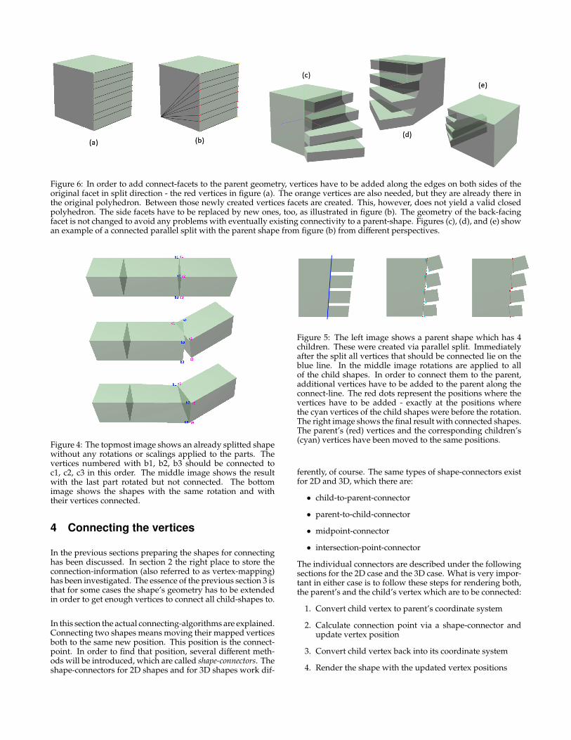
Figure 6: In order to add connect-facets to the parent geometry, vertices have to be added along the edges on both sides of theoriginal facet in split direction - the red vertices in figure (a). The orange vertices are also needed, but they are already there inthe original polyhedron. Between those newly created vertices facets are created. This, however, does not yield a valid closedpolyhedron. The side facets have to be replaced by new ones, too, as illustrated in figure (b). The geometry of the back-facingfacet is not changed to avoid any problems with eventually existing connectivity to a parent-shape. Figures (c), (d), and (e) showan example of a connected parallel split with the parent shape from figure (b) from different perspectives.

Figure 4: The topmost image shows an already splitted shapewithout any rotations or scalings applied to the parts. Thevertices numbered with b1, b2, b3 should be connected toc1, c2, c3 in this order. The middle image shows the resultwith the last part rotated but not connected. The bottomimage shows the shapes with the same rotation and withtheir vertices connected.

4 Connecting the vertices

In the previous sections preparing the shapes for connectinghas been discussed. In section 2 the right place to store theconnection-information (also referred to as vertex-mapping)has been investigated. The essence of the previous section 3 isthat for some cases the shape’s geometry has to be extendedin order to get enough vertices to connect all child-shapes to.

In this section the actual connecting-algorithms are explained.Connecting two shapes means moving their mapped verticesboth to the same new position. This position is the connect-point. In order to find that position, several different meth-ods will be introduced, which are called shape-connectors. Theshape-connectors for 2D shapes and for 3D shapes work dif-

Figure 5: The left image shows a parent shape which has 4children. These were created via parallel split. Immediatelyafter the split all vertices that should be connected lie on theblue line. In the middle image rotations are applied to allof the child shapes. In order to connect them to the parent,additional vertices have to be added to the parent along theconnect-line. The red dots represent the positions where thevertices have to be added - exactly at the positions wherethe cyan vertices of the child shapes were before the rotation.The right image shows the final result with connected shapes.The parent’s (red) vertices and the corresponding children’s(cyan) vertices have been moved to the same positions.

ferently, of course. The same types of shape-connectors existfor 2D and 3D, which there are:

• child-to-parent-connector

• parent-to-child-connector

• midpoint-connector

• intersection-point-connector

The individual connectors are described under the followingsections for the 2D case and the 3D case. What is very impor-tant in either case is to follow these steps for rendering both,the parent’s and the child’s vertex which are to be connected:

1. Convert child vertex to parent’s coordinate system

2. Calculate connection point via a shape-connector andupdate vertex position

3. Convert child vertex back into its coordinate system

4. Render the shape with the updated vertex positions

Connecting a 2D shape

Three connector-types are quite easy to implement. Theparent-to-child-connector simply moves the parent vertex to thechild vertex position.The child-to-parent-connector moves the child vertex to the par-ent vertex position.And the midpoint-connector calculates the point which is inthe middle of the parent vertex and the child vertex using theformula:

~m =

( px+cx2py+cy2

)(1)

where ~m is the midpoint, p is the parent vertex, and c isthe child vertex, each of the vertices is represented by a2-dimensional vector.

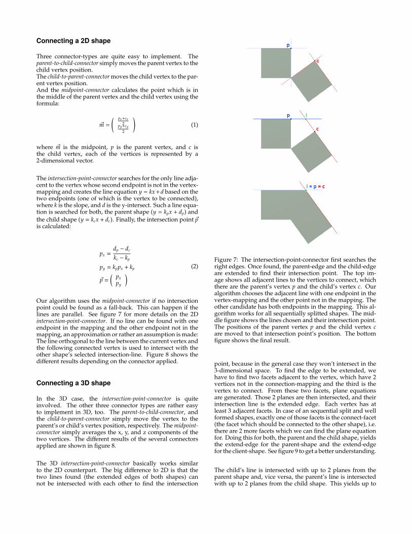
The intersection-point-connector searches for the only line adja-cent to the vertex whose second endpoint is not in the vertex-mapping and creates the line equation y = kx+d based on thetwo endpoints (one of which is the vertex to be connected),where k is the slope, and d is the y-intersect. Such a line equa-tion is searched for both, the parent shape (y = kpx + dp) andthe child shape (y = kcx + dc). Finally, the intersection point ~pis calculated:

px =dp − dc

kc − kp

py = kppx + kp

~p =(

pxpy

) (2)

Our algorithm uses the midpoint-connector if no intersectionpoint could be found as a fall-back. This can happen if thelines are parallel. See figure 7 for more details on the 2Dintersection-point-connector. If no line can be found with oneendpoint in the mapping and the other endpoint not in themapping, an approximation or rather an assumption is made:The line orthogonal to the line between the current vertex andthe following connected vertex is used to intersect with theother shape’s selected intersection-line. Figure 8 shows thedifferent results depending on the connector applied.

Connecting a 3D shape

In the 3D case, the intersection-point-connector is quiteinvolved. The other three connector types are rather easyto implement in 3D, too. The parent-to-child-connector, andthe child-to-parent-connector simply move the vertex to theparent’s or child’s vertex position, respectively. The midpoint-connector simply averages the x, y, and z components of thetwo vertices. The different results of the several connectorsapplied are shown in figure 8.

The 3D intersection-point-connector basically works similarto the 2D counterpart. The big difference to 2D is that thetwo lines found (the extended edges of both shapes) cannot be intersected with each other to find the intersection

Figure 7: The intersection-point-connector first searches theright edges. Once found, the parent-edge and the child-edgeare extended to find their intersection point. The top im-age shows all adjacent lines to the vertices to connect, whichthere are the parent’s vertex p and the child’s vertex c. Ouralgorithm chooses the adjacent line with one endpoint in thevertex-mapping and the other point not in the mapping. Theother candidate has both endpoints in the mapping. This al-gorithm works for all sequentially splitted shapes. The mid-dle figure shows the lines chosen and their intersection point.The positions of the parent vertex p and the child vertex care moved to that intersection point’s position. The bottomfigure shows the final result.

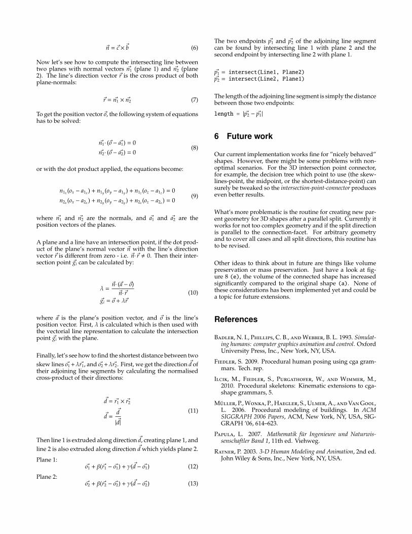
point, because in the general case they won’t intersect in the3-dimensional space. To find the edge to be extended, wehave to find two facets adjacent to the vertex, which have 2vertices not in the connection-mapping and the third is thevertex to connect. From these two facets, plane equationsare generated. Those 2 planes are then intersected, and theirintersection line is the extended edge. Each vertex has atleast 3 adjacent facets. In case of an sequential split and wellformed shapes, exactly one of those facets is the connect-facet(the facet which should be connected to the other shape), i.e.there are 2 more facets which we can find the plane equationfor. Doing this for both, the parent and the child shape, yieldsthe extend-edge for the parent-shape and the extend-edgefor the client-shape. See figure 9 to get a better understanding.

The child’s line is intersected with up to 2 planes from theparent shape and, vice versa, the parent’s line is intersectedwith up to 2 planes from the child shape. This yields up to

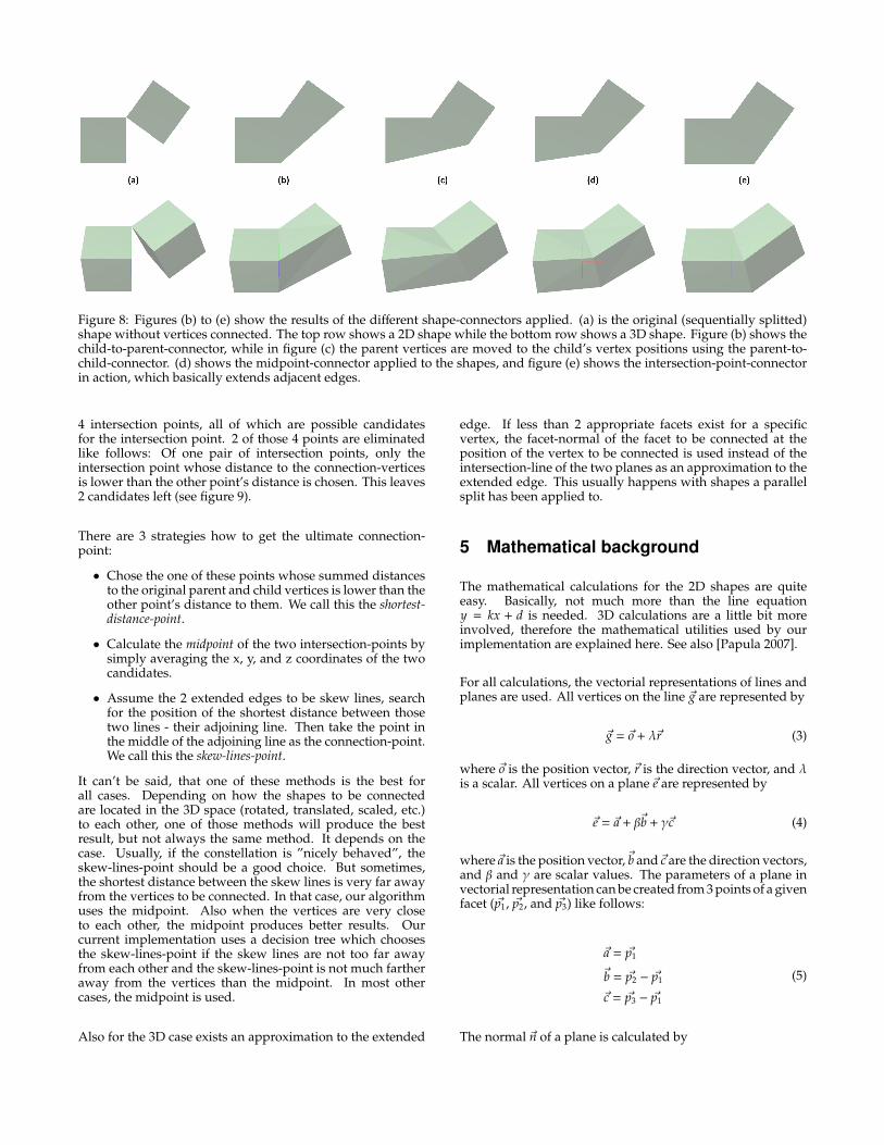
Figure 8: Figures (b) to (e) show the results of the different shape-connectors applied. (a) is the original (sequentially splitted)shape without vertices connected. The top row shows a 2D shape while the bottom row shows a 3D shape. Figure (b) shows thechild-to-parent-connector, while in figure (c) the parent vertices are moved to the child’s vertex positions using the parent-to-child-connector. (d) shows the midpoint-connector applied to the shapes, and figure (e) shows the intersection-point-connectorin action, which basically extends adjacent edges.

4 intersection points, all of which are possible candidatesfor the intersection point. 2 of those 4 points are eliminatedlike follows: Of one pair of intersection points, only theintersection point whose distance to the connection-verticesis lower than the other point’s distance is chosen. This leaves2 candidates left (see figure 9).

There are 3 strategies how to get the ultimate connection-point:

• Chose the one of these points whose summed distancesto the original parent and child vertices is lower than theother point’s distance to them. We call this the shortest-distance-point.

• Calculate the midpoint of the two intersection-points bysimply averaging the x, y, and z coordinates of the twocandidates.

• Assume the 2 extended edges to be skew lines, searchfor the position of the shortest distance between thosetwo lines - their adjoining line. Then take the point inthe middle of the adjoining line as the connection-point.We call this the skew-lines-point.

It can’t be said, that one of these methods is the best forall cases. Depending on how the shapes to be connectedare located in the 3D space (rotated, translated, scaled, etc.)to each other, one of those methods will produce the bestresult, but not always the same method. It depends on thecase. Usually, if the constellation is ”nicely behaved”, theskew-lines-point should be a good choice. But sometimes,the shortest distance between the skew lines is very far awayfrom the vertices to be connected. In that case, our algorithmuses the midpoint. Also when the vertices are very closeto each other, the midpoint produces better results. Ourcurrent implementation uses a decision tree which choosesthe skew-lines-point if the skew lines are not too far awayfrom each other and the skew-lines-point is not much fartheraway from the vertices than the midpoint. In most othercases, the midpoint is used.

Also for the 3D case exists an approximation to the extended

edge. If less than 2 appropriate facets exist for a specificvertex, the facet-normal of the facet to be connected at theposition of the vertex to be connected is used instead of theintersection-line of the two planes as an approximation to theextended edge. This usually happens with shapes a parallelsplit has been applied to.

5 Mathematical background

The mathematical calculations for the 2D shapes are quiteeasy. Basically, not much more than the line equationy = kx + d is needed. 3D calculations are a little bit moreinvolved, therefore the mathematical utilities used by ourimplementation are explained here. See also [Papula 2007].

For all calculations, the vectorial representations of lines andplanes are used. All vertices on the line ~g are represented by

~g = ~o + λ~r (3)

where ~o is the position vector, ~r is the direction vector, and λis a scalar. All vertices on a plane ~e are represented by

~e = ~a + β~b + γ~c (4)

where~a is the position vector,~b and~c are the direction vectors,and β and γ are scalar values. The parameters of a plane invectorial representation can be created from 3 points of a givenfacet (~p1, ~p2, and ~p3) like follows:

~a = ~p1

~b = ~p2 − ~p1

~c = ~p3 − ~p1

(5)

The normal ~n of a plane is calculated by

~n = ~c ×~b (6)

Now let’s see how to compute the intersecting line betweentwo planes with normal vectors ~n1 (plane 1) and ~n2 (plane2). The line’s direction vector ~r is the cross product of bothplane-normals:

~r = ~n1 × ~n2 (7)

To get the position vector ~o, the following system of equationshas to be solved:

~n1· (~o − ~a1) = 0

~n2· (~o − ~a2) = 0(8)

or with the dot product applied, the equations become:

n1x (ox − a1x ) + n1y (oy − a1y ) + n1z (oz − a1z ) = 0

n2x (ox − a2x ) + n2y (oy − a2y ) + n2z (oz − a2z ) = 0(9)

where ~n1 and ~n2 are the normals, and ~a1 and ~a2 are theposition vectors of the planes.

A plane and a line have an intersection point, if the dot prod-uct of the plane’s normal vector ~n with the line’s directionvector ~r is different from zero - i.e. ~n·~r , 0. Then their inter-section point ~gi can be calculated by:

λ =~n· (~a − ~o)~n·~r

~gi = ~o + λ~r(10)

where ~a is the plane’s position vector, and ~o is the line’sposition vector. First, λ is calculated which is then used withthe vectorial line representation to calculate the intersectionpoint ~gi with the plane.

Finally, let’s see how to find the shortest distance between twoskew lines ~o1 +λ~r1, and ~o2 +λ~r2. First, we get the direction ~d oftheir adjoining line segments by calculating the normalisedcross-product of their directions:

~d = ~r1 × ~r2

~d =~d

|~d|

(11)

Then line 1 is extruded along direction ~d, creating plane 1, andline 2 is also extruded along direction ~d which yields plane 2.

Plane 1:~o1 + β(~r1 − ~o1) + γ(~d − ~o1) (12)

Plane 2:~o2 + β(~r2 − ~o2) + γ(~d − ~o2) (13)

The two endpoints ~p1 and ~p2 of the adjoining line segmentcan be found by intersecting line 1 with plane 2 and thesecond endpoint by intersecting line 2 with plane 1.

~p1 = intersect(Line1, Plane2)~p2 = intersect(Line2, Plane1)

The length of the adjoining line segment is simply the distancebetween those two endpoints:

length = |~p2 − ~p1|

6 Future work

Our current implementation works fine for ”nicely behaved”shapes. However, there might be some problems with non-optimal scenarios. For the 3D intersection point connector,for example, the decision tree which point to use (the skew-lines-point, the midpoint, or the shortest-distance-point) cansurely be tweaked so the intersection-point-connector produceseven better results.

What’s more problematic is the routine for creating new par-ent geometry for 3D shapes after a parallel split. Currently itworks for not too complex geometry and if the split directionis parallel to the connection-facet. For arbitrary geometryand to cover all cases and all split directions, this routine hasto be revised.

Other ideas to think about in future are things like volumepreservation or mass preservation. Just have a look at fig-ure 8 (e), the volume of the connected shape has increasedsignificantly compared to the original shape (a). None ofthese considerations has been implemented yet and could bea topic for future extensions.

References

Badler, N. I., Phillips, C. B., andWebber, B. L. 1993. Simulat-ing humans: computer graphics animation and control. OxfordUniversity Press, Inc., New York, NY, USA.

Fiedler, S. 2009. Procedural human posing using cga gram-mars. Tech. rep.

Ilcik, M., Fiedler, S., Purgathofer, W., and Wimmer, M.,2010. Procedural skeletons: Kinematic extensions to cga-shape grammars, 5.

Muller, P., Wonka, P., Haegler, S., Ulmer, A., andVanGool,L. 2006. Procedural modeling of buildings. In ACMSIGGRAPH 2006 Papers, ACM, New York, NY, USA, SIG-GRAPH ’06, 614–623.

Papula, L. 2007. Mathematik fur Ingenieure und Naturwis-senschaftler Band 1, 11th ed. Viehweg.

Ratner, P. 2003. 3-D Human Modeling and Animation, 2nd ed.John Wiley & Sons, Inc., New York, NY, USA.

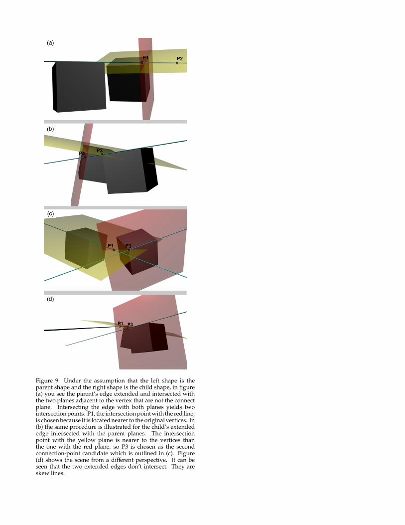
Figure 9: Under the assumption that the left shape is theparent shape and the right shape is the child shape, in figure(a) you see the parent’s edge extended and intersected withthe two planes adjacent to the vertex that are not the connectplane. Intersecting the edge with both planes yields twointersection points. P1, the intersection point with the red line,is chosen because it is located nearer to the original vertices. In(b) the same procedure is illustrated for the child’s extendededge intersected with the parent planes. The intersectionpoint with the yellow plane is nearer to the vertices thanthe one with the red plane, so P3 is chosen as the secondconnection-point candidate which is outlined in (c). Figure(d) shows the scene from a different perspective. It can beseen that the two extended edges don’t intersect. They areskew lines.