International Journal of Heat and Mass Transfer 66 (2013) 489–495

Contents lists available at ScienceDirect

International Journal of Heat and Mass Transfer

journal homepage: www.elsevier .com/locate / i jhmt

Conjugate heat transfer in a plate – One surface at constant temperatureand the other cooled by forced or natural convection

0017-9310/$ - see front matter � 2013 Elsevier Ltd. All rights reserved.http://dx.doi.org/10.1016/j.ijheatmasstransfer.2013.07.052

⇑ Corresponding author. Tel.: +358 408490970.E-mail addresses: matti.lindstedt@tut.fi (M. Lindstedt), reijo.karvinen@tut.fi (R.

Karvinen).

Matti Lindstedt, Reijo Karvinen ⇑Tampere University of Technology, P.O. Box 589, 33101 Tampere, Finland

a r t i c l e i n f o a b s t r a c t

Article history:Received 22 April 2013Received in revised form 4 July 2013Accepted 22 July 2013Available online 15 August 2013

Keywords:Flat plateConjugate heat transferForced convectionNatural convection

Simple analytical solutions for the steady-state total heat transfer rate are presented for a flat plate cooledon one surface by forced or natural convection while the other side remains at uniform temperature.These solutions are also used to determine the unknown interface temperature of the surface. The solu-tions are based on one-dimensional conduction in the plate and on the heat transfer coefficients of anisothermal surface. The results are compared with those in the literature combined with a brief discus-sion of the most relevant studies in the field. In addition, presented are also numerically calculated resultsthat take into account two-dimensional conduction in the plate and the effect of non-uniform surfacetemperature on convection. The calculations show that the results are valid also for thick plates. The solu-tion procedure proved very accurate and produced new simple results for engineering applications.

� 2013 Elsevier Ltd. All rights reserved.

1. Introduction

In conjugate heat transfer problems, a simultaneous solution isrequired for heat conduction in a solid and convection to an adja-cent fluid because neither the temperature distribution nor theheat flux at the solid–fluid interface is known a priori, yet they con-tribute to solving the problem. Though the literature on conjugateheat transfer dates back to the 1960s’, Dorfman’s [1] recent book isthe first comprehensive work on existing studies.

The most interesting feature in solving conjugate heat transferproblems in, for example, electronics cooling systems is usuallythe relationship between the total heat transfer rate and the max-imum temperature. In general, if boundary conditions are specifiedfor temperature, the total heat transfer rate is of interest. On theother hand, with a specified heat input, the total heat transfer rateis known and the maximum temperature should be determined.

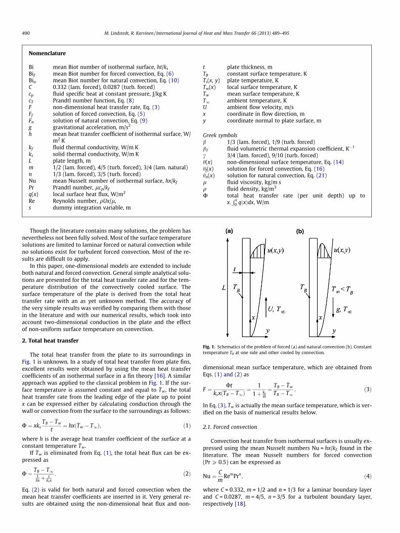
Perhaps the best known conjugate heat transfer problem is thatof Perelman [2] and Luikov [3], in which one side of the plate re-mains at a constant temperature while the other is heated or cooledby forced laminar convection (illustrated schematically in Fig. 1a forforced convection and in Fig. 1b for natural convection). As a resultof non-uniform cooling, the temperature distribution on the platesurface remains unknown, as does the total heat transfer rate.

The distribution of the surface temperature in the plate inFig. 1a with laminar forced convection has frequently been studied.For example, Payvar [4], Karvinen [5], and Mosaad [6] used integral

boundary layer methods for convection and assumed a linear tem-perature profile across the plate thickness, ignoring stream-wiseheat conduction. Trevino et al. [7] developed an analytical equationfor total heat flux when the plate is close to isothermal. Because oftheir convection models, all these studies are, in fact, valid for Pra-ndtl numbers larger than 0.5. Worth quoting are also the numericalresults of Chida [8], which took into accounttwo-dimensional con-duction in the plate. Most analytical results are valid only at largeor small Brun numbers, whereas only few sophisticated solutionsare valid everywhere [9].

Vynnycky and Kimura [10] made an important contribution tosolving the problem in Fig. 1b by developing an approximateone-dimensional model, which does not solve the boundary layerequations at all but rather assumes the surface to be isothermaland uses the heat transfer coefficient of natural convection froman isothermal surface. Their results were experimentally verifiedby Kimura et al. [11] for three plates with different material prop-erties using water for fluid. Vynnycky et al. [12] developed a corre-sponding one-dimensional model for the total heat transfer rate inforced convection, which introduced a connection between themean surface temperature and the total heat transfer rate.

Natural convection has mostly been treated numerically bysolving the boundary layer equations. Merkin and Pop [13] pre-sented such a solution using an iterative finite-difference schemewhereas Yu and Lin solved the boundary layer equations numeri-cally and presented a correlation for the surface temperature[14]. The effect of stream-wise conduction in the plate has beennumerically studied by Miyamoto et al. [15], who also proposeda simple model for the surface temperature, based on the heattransfer coefficient of an isothermal surface.

Nomenclature

Bi mean Biot number of isothermal surface, ht/ks

Bif mean Biot number for forced convection, Eq. (6)Bin mean Biot number for natural convection, Eq. (10)C 0.332 (lam. forced), 0.0287 (turb. forced)cp fluid specific heat at constant pressure, J/kg KcT Prandtl number function, Eq. (8)F non-dimensional heat transfer rate, Eq. (3)Ff solution of forced convection, Eq. (5)Fn solution of natural convection, Eq. (9)g gravitational acceleration, m/s2

h mean heat transfer coefficient of isothermal surface, W/m2 K

kf fluid thermal conductivity, W/m Kks solid thermal conductivity, W/m KL plate length, mm 1/2 (lam. forced), 4/5 (turb. forced), 3/4 (lam. natural)n 1/3 (lam. forced), 3/5 (turb. forced)Nu mean Nusselt number of isothermal surface, hx/kf

Pr Prandtl number, lcp/kf

q(x) local surface heat flux, W/m2

Re Reynolds number, qUx/l,s dummy integration variable, m

t plate thickness, mTB constant surface temperature, KTs(x, y) plate temperature, KTw(x) local surface temperature, K�Tw mean surface temperature, KT1 ambient temperature, KU ambient flow velocity, m/sx coordinate in flow direction, my coordinate normal to plate surface, m

Greek symbolsb 1/3 (lam. forced), 1/9 (turb. forced)bT fluid volumetric thermal expansion coefficient, K�1

c 3/4 (lam. forced), 9/10 (turb. forced)h(x) non-dimensional surface temperature, Eq. (14)hf(x) solution for forced convection, Eq. (16)hn(x) solution for natural convection, Eq. (21)l fluid viscosity, kg/m sq fluid density, kg/m3

U total heat transfer rate (per unit depth) up tox;R x

0 qðxÞdx, W/m

Fig. 1. Schematics of the problem of forced (a) and natural convection (b). Constanttemperature TB at one side and other cooled by convection.

490 M. Lindstedt, R. Karvinen / International Journal of Heat and Mass Transfer 66 (2013) 489–495

Though the literature contains many solutions, the problem hasnevertheless not been fully solved. Most of the surface temperaturesolutions are limited to laminar forced or natural convection whileno solutions exist for turbulent forced convection. Most of the re-sults are difficult to apply.

In this paper, one-dimensional models are extended to includeboth natural and forced convection. General simple analytical solu-tions are presented for the total heat transfer rate and for the tem-perature distribution of the convectively cooled surface. Thesurface temperature of the plate is derived from the total heattransfer rate with an as yet unknown method. The accuracy ofthe very simple results was verified by comparing them with thosein the literature and with our numerical results, which took intoaccount two-dimensional conduction in the plate and the effectof non-uniform surface temperature on convection.

2. Total heat transfer

The total heat transfer from the plate to its surroundings inFig. 1 is unknown. In a study of total heat transfer from plate fins,excellent results were obtained by using the mean heat transfercoefficients of an isothermal surface in a fin theory [16]. A similarapproach was applied to the classical problem in Fig. 1. If the sur-face temperature is assumed constant and equal to �Tw, the totalheat transfer rate from the leading edge of the plate up to pointx can be expressed either by calculating conduction through thewall or convection from the surface to the surroundings as follows:

U ¼ xksTB � �Tw

t¼ hxð�Tw � T1Þ; ð1Þ

where h is the average heat transfer coefficient of the surface at aconstant temperature �Tw.

If �Tw is eliminated from Eq. (1), the total heat flux can be ex-pressed as

U ¼ TB � T11hxþ t

ksx

: ð2Þ

Eq. (2) is valid for both natural and forced convection when themean heat transfer coefficients are inserted in it. Very general re-sults are obtained using the non-dimensional heat flux and non-

dimensional mean surface temperature, which are obtained fromEqs. (1) and (2) as

F ¼ UtksxðTB � T1Þ

¼ 11þ ks

th

¼ TB � �Tw

TB � T1; ð3Þ

In Eq. (3), �Tw is actually the mean surface temperature, which is ver-ified on the basis of numerical results below.

2.1. Forced convection

Convection heat transfer from isothermal surfaces is usually ex-pressed using the mean Nusselt numbers Nu = hx/kf, found in theliterature. The mean Nusselt numbers for forced convection(Pr P 0.5) can be expressed as

Nu ¼ Cm

RemPrn; ð4Þ

where C = 0.332, m = 1/2 and n = 1/3 for a laminar boundary layerand C = 0.0287, m = 4/5, n = 3/5 for a turbulent boundary layer,respectively [18].

M. Lindstedt, R. Karvinen / International Journal of Heat and Mass Transfer 66 (2013) 489–495 491

When the heat transfer coefficient from Eq. (4) is inserted in Eq.(3) and the mean Biot number Bif = ht/ks is adopted, the non-dimensional heat flux can be written as

Ff ¼1

1þ 1Bif

; ð5Þ

where the subscript f refers to forced convection and the mean Biotnumber is

Bif ¼Cm

RemPrn kf tksx

: ð6Þ

An equation similar to Eq. (5) was derived in Ref. [12] using a moresophisticated method and different variables than in the present pa-per. Note that in Eq. (5) x is the total plate length, that is, x = L inFig. 1.

Results of conjugate heat transfer from a flat plate have usuallybeen given as a function of the Brun number. We present themusing the Biot number in Eq. (6), which, in fact, is the same asthe Brun number multiplied by a constant C/m.

2.2. Natural convection

The mean Nusselt number of a vertical constant temperaturesurface with a laminar boundary layer is [17]

Nu ¼ 43

cTgbTq2ð�Tw � T1Þx3

l2

� �1=4

; ð7Þ

where the Prandtl number dependency is

cT ¼ 0:503Pr1=4 1þ 0:492Pr

� �9=16" #�4=9

: ð8Þ

According to Eq. (7), the heat transfer coefficient depends also onthe temperature difference between the surface and itssurroundings.

When the mean heat transfer coefficient obtained from Eq. (7)is inserted in Eq. (3) and when ð�Tw � T1Þ=ðTB � T1Þ ¼ 1� F is ta-ken into account, the total non-dimensional heat flux in Eq. (3)takes an implicit form as follows:

Fn

ð1� FnÞ5=4 ¼ Bin; ð9Þ

where the subscript n refers to natural convection. Evaluation of themean heat transfer coefficient in the Biot number in Eq. (7) is nowbased on the temperature difference TB � T1 and the result is

Bin ¼43

cTgbTq2ðTB � T1Þx3

l2

� �1=4 kf tksx

: ð10Þ

Equations for natural convection similar to those of Eq. (9) canbe found in the literature, though they have been derived in amuch more sophisticated way [10,11]. In the case of natural con-vection with a turbulent boundary layer, the heat transfer coef-ficient is almost independent of the stream-wise direction anddepends only on the temperature difference [17]. Consequently,the problem in Fig. 1b is easy to solve [11] and thus not dis-cussed here.

3. Surface temperature distribution

The above results of total heat transfer were based on theassumption of a constant surface temperature and the mean heattransfer coefficient of an isothermal surface. Of course, such a mod-el does not directly give the actual surface temperature variation.

When solving the surface temperature distribution, we ignorethe stream-wise heat conduction in the plate. Thus we have a par-abolic problem, and we can now calculate the local surface temper-ature by differentiating the mean surface temperature. The meansurface temperature from the leading edge up to point x is

�TwðxÞ ¼1x

Z x

0TwðsÞds: ð11Þ

By multiplying Eq. (11) by x and then differentiating it with respectto x, we obtain the local plate temperature as a function of the meantemperature

TwðxÞ ¼ �TwðxÞ þ xd�TwðxÞ

dx: ð12Þ

Eq. (12) can be presented in a non-dimensional form with the helpof Eq. (3)

hðxÞ ¼ F þ xdFdx; ð13Þ

where F is the non-dimensional total heat flux defined in Eq. (3).The non-dimensional local surface temperature is

hðxÞ ¼ TB � TwðxÞTB � T1

: ð14Þ

Eq. (13) can be expressed using the mean Biot number as a variableinstead of x. According to Eqs. (6) and (10), the mean Biot number isproportional to xm�1, where m is a constant depending on the flowtype and is given above for forced flow after Eq. (4). For natural con-vection, the value of m = 3/4 is obtained from Eq. (7). By changingthe variable from x to Bi, we get dx = x(m � 1)�1 Bi�1dBi andEq.(13) takes the form

hðxÞ ¼ F þ ðm� 1ÞBidFdBi

: ð15Þ

Eq. (15) is valid for both forced and natural convection because it issimply another way to express the relationship between local andmean surface temperature. In the sections below, expressions forlocal surface temperature are derived from Eq. (15) for differenttypes of convection by replacing F with non-dimensional heat fluxesFf and Fn in Eqs. (5) and (9).

3.1. Forced convection

Eq. (5) expresses F for forced convection to be used in Eq. (15).By inserting it in Eq. (15) and by performing the derivation, we ob-tain the surface temperature distribution

hf ðxÞ ¼Bif ðmþ Bif Þð1þ Bif Þ2

; ð16Þ

where the Biot number is defined in Eq. (6)

3.2. Natural convection

An implicit solution for the total heat transfer rate Fn is givenby Eq. (9). Differentiating Fn(Bin) with respect to Bin in Eq. (15)can be circumvented by differentiating the known inverse func-tion Bin(Fn) with respect to Fn and by taking the inverse of theresult

hnðxÞ ¼ Fn þ ðm� 1ÞBindBin

dFn

� ��1

: ð17Þ

The derivative inside the parentheses is now (m = 3/4)

dBin

dFn¼ Fn þ 4

4ð1� FnÞ9=4 : ð18Þ

492 M. Lindstedt, R. Karvinen / International Journal of Heat and Mass Transfer 66 (2013) 489–495

Combining Eqs. (17) and (18), we get the local surface temperatureas a function of the mean surface temperature or total heat transferrate

hnðxÞ ¼ Fn3þ 2Fn

4þ Fn: ð19Þ

The non-dimensional heat transfer rate Fn can be solved from Eq.(19) as a positive root of the solution of a quadratic equation. Theresult is

Fn ¼14

hnðxÞ � 3þffiffiffiffiffiffiffiffiffiffiffiffiffiffiffiffiffiffiffiffiffiffiffiffiffiffiffiffiffiffiffiffiffiffiffiffiffiffiffiffiffiffiffiffi9þ 26hnðxÞ þ hnðxÞ2

q� �: ð20Þ

By inserting Fn from Eq. (20) in Eq. (9), we finally get an implicitequation for the surface temperature in natural convection

Bin ¼ffiffiffi2p hnðxÞ � 3þ

ffiffiffiffiffiffiffiffiffiffiffiffiffiffiffiffiffiffiffiffiffiffiffiffiffiffiffiffiffiffiffiffiffiffiffiffiffiffiffiffiffiffiffiffi9þ 26hnðxÞ þ hnðxÞ2

q7� hnðxÞ �

ffiffiffiffiffiffiffiffiffiffiffiffiffiffiffiffiffiffiffiffiffiffiffiffiffiffiffiffiffiffiffiffiffiffiffiffiffiffiffiffiffiffiffiffi9þ 26hnðxÞ þ hnðxÞ2

q� �5=4 : ð21Þ

The value of the Biot number is obtained from Eq. (10). The non-dimensional surface temperature hn(x) can be solved by iterationfrom Eq. (21) after the mean Biot number has been determinedon the basis of the plate geometry and flow properties.

4. Numerical modeling

As mentioned above, the problems in Fig. 1 have been exten-sively studied over many decades with various methods. Depend-ing on the geometry and thermal properties of the fluid and plate,both stream-wise and transverse heat conduction may also affectthe temperature distribution and total heat transfer rate. Presentedbelow is a method for studying the effect of 2D heat conduction.

The plate temperature Ts(x, y) is governed by the heat conduc-tion equation

@2Tsðx; yÞ@x2 þ @

2Tsðx; yÞ@y2 ¼ 0: ð22Þ

With adiabatic plate edges, the boundary conditions are

Tsðx;�tÞ ¼ TB

@Tsð0; yÞ@x

¼ @TsðL; yÞ@x

¼ 0

� ks@Tsðx;0Þ

@y¼ qðxÞ;

ð23Þ

where q(x) is the convective heat flux between wall surface andenvironment.

For forced convection, the heat flux from the wall surface in Fig. 1with an arbitrary surface temperature can be obtained accuratelyfrom the equation

qðxÞ ¼ Ckf

xRemPrn TwðxÞ � T1 þ

Z x

01� s

x

� �c� ��b

@TwðsÞ@s

ds

" #;

ð24Þ

where Tw(x) is equal to Ts(x, 0) in Eq. (22). Eq. (24) is derived usingan integral method and a superposing technique for arbitrarilyvarying surface temperature (derivation available in [1,18]). Thevalues of the constants C, m, and n, c, and b for laminar and turbu-lent boundary layer flows are given in the nomenclature.

Natural convection from a non-isothermal vertical surface ismore difficult to deal with than forced convection. The firstapproximate solution to couple arbitrarily varying surface temper-ature and heat flux was developed by Raithby and Hollands [19],who used the analogy of film condensation and the boundary layerof natural convection near the surface. Later on, Lee and Yovano-

vich studied the problem of a non-isothermal surface by calculat-ing an induced free stream velocity which is analogous to theforced convection case. They derived the equation [20]

qðxÞ ¼ cTkf

x1=2

gbTq2

l2

� �1=4 Z x

0TwðsÞ � T1ds

� �

� TwðxÞ � T1 þZ x

01� s

x

� �9=8� ��11=24

@TwðsÞ@s

ds

!: ð25Þ

An influence function of the type [1 � (s/x)9/8]�11/24 was adoptedfrom the forced convection solution. The exponents 9/8 and 11/24were found by using numerical and analytical results of naturalconvection for Pr = 0.7. Eq. (25) gives an exact solution to constanttemperature and also to a constant heat flux boundary condition,where the surface temperature varies as (Tw(x) � T1) � x1/5.

Our computational method was based on a finite volume ap-proach, according to which the plate was divided into finite rectan-gular volumes in the x- and y-directions, and temperature wasspecified at the center of each volume. The grid size was400 � 20 for forced and 1000 � 20 for natural convection, that is,fine enough to yield a grid-independent solution in all studiedcases.

Eq. (22) is integrated over the volumes and leads to an algebraicequation for each volume. The boundary condition on the surface iscalculated by integrating the heat flux from Eqs. (24) and (25). Thesolution procedure involves sequential solving of the set of alge-braic equations for the plate temperature and then calculatingthe convective heat flux from the surface, which is the boundarycondition for a new iteration round. The process is repeated untilthe residuals of the governing heat conduction equation (22) areless than 10�9.

5. Results

The results of our analytical equations above are presentedgraphically and compared with existing results in the literatureand with our numerical results. In numerical calculations, thetwo-dimensional heat conduction equation was solved for theplate, and convection from a non-isothermal surface was takeninto account for forced flow and natural convection.

The thermal and flow properties of the numerical results inFigs. 2–5 were selected in such a way as to be realistic in practiceand for the variation in surface temperature to be visible. Innumerically calculated results for laminar flow a lower thermalconductivity is used than in the case of turbulent flow in order tobetter illustrate the results near leading edge. The material withthe lowest thermal conductivity is used with natural convection.

5.1. Total heat transfer rate

Fig. 2 shows analytical non-dimensional total heat transfer ratesfor different flow types together with numerical results. Non-dimensional heat transfer rates are given for the whole plate usingF = U t(ksL(TB � T1))�1, that is, x = L is used to define F for bothforced and natural convection.

Eq. (5) is valid for laminar and turbulent forced convection, butit must be noted that the constants in the mean Biot number in Eq.(6) are different for laminar and turbulent flows. With natural con-vection, Eq. (9) gives the heat transfer rate whereas the mean Biotnumber is obtained from Eq. (10).

In Fig. 2, numerically obtained results are almost the same asanalytical solutions; furthermore, the plate geometry does not af-fect them because the former, in three different plate length tothickness ratios L/t, agree with the latter. For laminar and turbulentforced convection, numerical solutions are the same. Fig. 2 alsoshows the asymptotic solution of Treviño et al. [7] for laminar

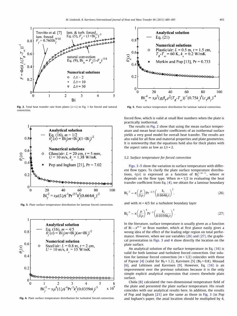
Fig. 2. Total heat transfer rate from plates (x = L) in Fig. 1 for forced and naturalconvection.

Fig. 3. Plate surface temperature distribution for laminar forced convection.

Fig. 4. Plate surface temperature distribution for turbulent forced convection.

Fig. 5. Plate surface temperature distribution for laminar natural convection.

M. Lindstedt, R. Karvinen / International Journal of Heat and Mass Transfer 66 (2013) 489–495 493

forced flow, which is valid at small Biot numbers when the plate ispractically isothermal.

The results in Fig. 2 show that using the mean surface temper-ature and mean heat transfer coefficients of an isothermal surfaceyields a very good model for overall heat transfer. The results arealso valid for all flow and material properties and plate geometries.It is noteworthy that the equations hold also for thick plates withthe aspect ratio as low as L/t = 2.

5.2. Surface temperature for forced convection

Figs. 3–5 show the variation in surface temperature with differ-ent flow types. To clarify the plate surface temperature distribu-tions, hf(x) is expressed as a function of Bi1=ðm�1Þ

f , where mdepends on the flow type. When m = 1/2 in evaluating the heattransfer coefficient from Eq. (4), we obtain for a laminar boundary

Bi�2f ¼ x

lUq

� �Pr�2=3 ks

0:664kf t

� �2

; ð26Þ

and with m = 4/5 for a turbulent boundary layer

Bi�5f ¼ x

lUq

� �4

Pr�3 ks

0:0359kf t

� �5

: ð27Þ

In the literature, surface temperature is usually given as a functionof Bi � xm-1 or Brun number, which at first glance easily gives awrong idea of the effect of the leading edge region on total perfor-mance. However, when we use variables (26) and (27), the graphi-cal presentation in Figs. 3 and 4 show directly the location on theplate surface.

An analytical solution of the surface temperature in Eq. (16) isvalid for both laminar and turbulent forced convection. Our solu-tion for laminar forced convection (m = 1/2) coincides with thoseof Payvar [4] (valid for Bif > 1.2), Karvinen [5] (Bif > 0.8), Mosaad[6], and Lehtinen and Karvinen [9]. However, Eq. (16) is animprovement over the previous solutions because it is the onlysimple explicit analytical expression that covers thewhole platesurface.

Chida [8] calculated the two-dimensional temperature field ofthe plate and presented the plate surface temperature. His resultcoincides with our analytical results here. In addition, the resultsof Pop and Ingham [21] are the same as those in Fig. 3 (in Popand Ingham’s paper, the axial location should be multiplied by 4,

494 M. Lindstedt, R. Karvinen / International Journal of Heat and Mass Transfer 66 (2013) 489–495

as also observed by Chida). This correction is included in the datain Fig. 3.

The effect of stream-wise heat conduction in the plate was ta-ken into account in two-dimensional calculations, performed usingthe solution procedure described above. Results of one example areshown in Fig. 3 for a glass plate of length L = 0.2 m and thicknesst = 5 mm in an air flow of velocity U = 10 m/s. In all numerical cal-culations, air properties were taken at T = 330 K. Clearly, thenumerically calculated temperature distribution follows well theanalytical solution. When in Fig. 3 the horizontal variable is Bi�2

f ,it also shows directly the location x on the plate surface. Withtwo-dimensional heat conduction, the plate leading edge remainsabove the flow temperature even though boundary layer solutionsare used for convection.

Fig. 4 shows the corresponding surface temperature for a turbu-lent boundary layer, assuming the boundary layer is turbulentright from the leading edge. In practice, a turbulent boundary layercan be easily obtained by roughening the surface or by placing, forexample, a small-diameter cylinder in a free stream just before theleading edge. Besides the analytical result, Fig. 4 shows alsonumerical results on a steel plate cooled with air, according towhich the plate surface is practically isothermal. With turbulentflow, variation in temperature can be ignored, and the mean tem-perature obtained from Eqs. (3) and (5), that is, Tw ¼ TB � ðTB�T1Þ=ð1þ Bi�1

f Þ, can be assumed over the whole plate surface.Calculations of laminar and turbulent flows with several differ-

ent plate geometries and thermal properties show that stream-wise heat conduction in the plate is important only very near theleading edge. Thus, the effects of two-dimensional conductioncan be ignored, and Eq. (16) can be used over the whole plate.

5.3. Surface temperature for natural convection

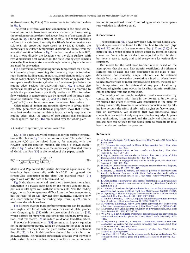
Eq. (21) is a new analytical expression for the surface tempera-ture of the plate in Fig. 1 with natural convection. The surface tem-perature hn(x) can be solved from it, for example, with theNewton–Raphson iteration method. The result is shown graphi-cally in Fig. 5, which shows also the numerically calculated resultsof Merkin and Pop [13] in the notation of this paper, namely

Bi�4n ¼ x

l2

gbTq2ðTB � T1Þ3ks

4cT kf t

� �4

: ð28Þ

Merkin and Pop solved the partial differential equations of theboundary layer numerically with Pr = 0.733 but ignored thestream-wise conduction in the plate. Our analytical result (21)agrees well with the data of Merkin and Pop.

Fig. 5 also shows numerical results with two-dimensional heatconduction in a plastic plate based on the method used in this pa-per; our results agree well with the other results. Near the leadingedge, the surface temperature differs from the flow temperature,but the result of Eq. (21) deviates from numerical solutions onlyat a short distance from the leading edge. Thus, Eq. (21) can beused over the whole surface.

Fig. 5 shows that the plate surface temperature can be graphedin a single curve for all material properties and all plate geome-tries. Comparing Eq. (21) with the correlation of Yu and Lin [14],which is based on numerical solutions of the boundary layer equa-tions, confirms that Eq. (21) is, in fact, valid for all Prandtl numbers.

Previously, Miyamoto et al. [15] presented an implicit equationfor the surface temperature, based on the assumption that the localheat transfer coefficient on the plate surface could be obtainedfrom Eq. (7). In fact, in this problem the local heat transfer is notknown a priori. Their model is surprisingly accurate over the wholeplate surface because the heat transfer coefficient in natural con-

vection is proportional to �x�1/4, according to which the tempera-ture variation is relatively small.

6. Conclusions

The problems in Fig. 1 have now been fully solved. Simple ana-lytical expressions were found for the total heat transfer rate (Eqs.(5) and (9)) and the surface temperature (Eqs. (16) and (21)) of theplates in Fig. 1 when cooled or heated either by forced or naturalconvection. Some solutions, indeed, are reported in the literature,but none is easy to apply and valid everywhere for various flowsituations.

Our model for the total heat transfer rate is based on theassumptions that the mean heat transfer coefficients of isothermalsurfaces can be used, and that conduction in the plate is one–dimensional. Consequently, simple solutions can be obtainedthough for natural convection the solution is implicit. When the to-tal heat transfer rate or mean temperature is known, the local sur-face temperature can be obtained at any plate location bydifferentiating in the same way as the local heat transfer coefficientcan be obtained from the mean value.

The validity of our simple analytical results was verified bycomparing the results with those in the literature. Furthermore,we studied the effect of stream-wise conduction in the plate bysolving numerically two-dimensional heat conduction and by tak-ing into account the effect of arbitrarily varying surface tempera-ture on convection. We observed that two-dimensional heatconduction has an effect only very near the leading edge. In prac-tical applications, it can ignored, and the analytical solutions ex-pressed here can be used for the whole plate to calculate its totalheat transfer and surface temperature.

References

[1] A. Dorfman, Conjugate Problems in Convective Heat Transfer, CRC Press, BocaRaton, 2009.

[2] T.L. Perelman, On conjugated problems of heat transfer, Int. J. Heat MassTransfer 3 (1961) 293–303.

[3] A. Luikov, Conjugate convective heat transfer problems, Int. J. Heat MassTransfer 17 (1974) 257–267.

[4] P. Payvar, Convective heat transfer to laminar flow over a plate of finitethickness, Int. J. Heat Mass Transfer 20 (1977) 431–433.

[5] R. Karvinen, Note on conjugated heat transfer in a flat plate, Lett. Heat MassTransfer 5 (1978) 197–202.

[6] M. Mosaad, Laminar forced convection conjugate heat transfer over a flat plate,Heat Mass Transfer 35 (1999) 371–375.

[7] C. Treviño, G. Becerra, F. Méndez, The classical problem of convective heattransfer in laminar flow over a thin finite thickness plate with uniformtemperature at the lower surface, Int. J. Heat Mass Transfer 40 (1997) 3577–3580.

[8] K. Chida, Surface temperature of a flat plate of finite thickness under conjugatelaminar forced convection heat transfer condition, Int. J. Heat Mass Transfer 43(2000) 639–642.

[9] A. Lehtinen, R. Karvinen, Analytical solution for a class of flat plate conjugateconvective heat transfer problems, Front. Heat Mass Transfer 2 (2011). 043004.

[10] M. Vynnycky, S. Kimura, Conjugate free convection due to a heated verticalplate, Int. J. Heat Mass Transfer 39 (1996) 1067–1080.

[11] S. Kimura, A. Okajima, T. Kiwata, Conjugate natural convection from a verticalheated slab, Int. J. Heat Mass Transfer 41 (1998) 3203–3211.

[12] M. Vynnycky, S. Kimura, K. Kanev, I. Pop, Forced convection heat transfer froma flat plate: the conjugate problem, Int. J. Heat Mass Transfer 41 (1998) 45–49.

[13] J.H. Merkin, I. Pop, Conjugate free convection on a vertical surface, Int. J. HeatMass Transfer 39 (1996) 1527–1534.

[14] W.-S. Yu, H.-T. Lin, Conjugate problems of conduction and free convection onvertical and horizontal flat plates, Int. J. Heat Mass Transfer 36 (1993) 1303–1313.

[15] M. Miyamoto, J. Sumikawa, T. Akiyoshi, T. Nakamura, Effects of axial heatconduction in a vertical flat plate on free convection heat transfer, Int. J. HeatMass Transfer 23 (1980) 1545–1553.

[16] R. Karvinen, T. Karvinen, Optimum geometry of plate fins, ASME J. HeatTransfer 134 (2012) 081801.

[17] S.W. Churchill, H.H.S. Chu, Correlating equations for laminar and turbulent freeconvection from a vertical plate, Int. J. Heat Mass Transfer 18 (1975) 1323–1329.

M. Lindstedt, R. Karvinen / International Journal of Heat and Mass Transfer 66 (2013) 489–495 495

[18] W. Kays, M. Crawford, B. Weigand, Convective Heat and Mass Transfer, fourthed., McGraw-Hill, New York, 2005.

[19] G.D. Raithby, K.G.T. Hollands, A general method of obtaining approximatesolutions to laminar and turbulent free convection problems, Advances in HeatTransfer, vol. 11, Academic Press, New York, 1975, pp. 265–315.

[20] S. Lee, M.M. Yovanovich, Linearization method for buoyancy induced flow overa nonisothermal vertical plate, J. Thermophys. Heat Transfer 7 (1993) 158–164.

[21] I. Pop, D.B. Ingham, A note on conjugate forced convection boundary-layerflow past a flat plate, Int. J. Heat Mass Transfer 36 (1993) 3873–3876.