Embed Size (px)
Citation preview
Stochastics and Financial Mathematics MSc
Master Thesis
Conic Swaption Pricing with DisplacedSABR
Author: Supervisor:Loizos Raounas prof. dr. Asma Khedher
Examination date: Daily supervisor:October 17, 2018 dr. Jovanka Lukic
Korteweg-de Vries Institute forMathematics
ABN AMRO

2
Abstract
Conic Finance is a recently formulated financial theory, in which bid and ask prices are modelledand priced directly, as distorted expected values through some concave distortion function. Inthis study, we apply this theory in order to price the bid and ask values of USD and EURswaptions, using the stochastic volatility model SABR. Our results support the notion of ConicFinance as a solid financial framework, which not only does not contradict the classical risk-neutral framework, but in fact fully incorporates it as a special case.
Keywords: Conic Finance, Swaptions, bid and ask pricing, distortion function
Title: Conic Swaption Pricing with Displaced SABRAuthor: Loizos Raounas, [email protected], 11404302Supervisor: prof. dr. Asma Khedher, dr. Jovanka LukicSecond Examiner: prof. dr. Peter SpreijExamination date: October 17, 2018
Korteweg-de Vries Institute for MathematicsUniversity of AmsterdamScience Park 105-107, 1098 XG Amsterdamhttp://kdvi.uva.nl
ABN AMROGustav Mahlerlaan 10, 1082PP Amsterdamhttp://www.abnamro.nl
3

4

Στην Μητέρα.
5
Contents
Introduction 8
1 Conic Finance 101.1 Liquid Markets . . . . . . . . . . . . . . . . . . . . . . . . . . . . . . . . . . . 101.2 Coherent Risk Measures . . . . . . . . . . . . . . . . . . . . . . . . . . . . . . 121.3 Illiquid Markets . . . . . . . . . . . . . . . . . . . . . . . . . . . . . . . . . . . 161.4 No Arbitrage in different markets . . . . . . . . . . . . . . . . . . . . . . . . . 171.5 Distorted Expectations . . . . . . . . . . . . . . . . . . . . . . . . . . . . . . . 181.6 Examples of distortion functions . . . . . . . . . . . . . . . . . . . . . . . . . . 221.7 Conic Finance Pricing . . . . . . . . . . . . . . . . . . . . . . . . . . . . . . . 23
1.7.1 Conic Binomial Trees . . . . . . . . . . . . . . . . . . . . . . . . . . . . 231.7.2 Conic Monte Carlo . . . . . . . . . . . . . . . . . . . . . . . . . . . . . 25
2 Swaptions and the SABR model 282.1 Swaps . . . . . . . . . . . . . . . . . . . . . . . . . . . . . . . . . . . . . . . . 28
2.1.1 Single Curve Framework . . . . . . . . . . . . . . . . . . . . . . . . . . 282.1.2 Multi-Curve Framework . . . . . . . . . . . . . . . . . . . . . . . . . . 29
2.2 Swaptions . . . . . . . . . . . . . . . . . . . . . . . . . . . . . . . . . . . . . . 302.3 SABR . . . . . . . . . . . . . . . . . . . . . . . . . . . . . . . . . . . . . . . . 33
2.3.1 Original SABR Model . . . . . . . . . . . . . . . . . . . . . . . . . . . 332.3.2 Negative Interest Rates SABR adaptations . . . . . . . . . . . . . . . . 35
3 Methodology 373.1 Data . . . . . . . . . . . . . . . . . . . . . . . . . . . . . . . . . . . . . . . . . 37
3.1.1 Cash Settled (EUR) . . . . . . . . . . . . . . . . . . . . . . . . . . . . 373.1.2 Swap Settled (USD) . . . . . . . . . . . . . . . . . . . . . . . . . . . . 38
3.2 Calibration . . . . . . . . . . . . . . . . . . . . . . . . . . . . . . . . . . . . . . 383.3 Simulation . . . . . . . . . . . . . . . . . . . . . . . . . . . . . . . . . . . . . . 39
3.3.1 Euler Scheme . . . . . . . . . . . . . . . . . . . . . . . . . . . . . . . . 403.3.2 Semi-Exact . . . . . . . . . . . . . . . . . . . . . . . . . . . . . . . . . 41
3.4 Bid and Ask . . . . . . . . . . . . . . . . . . . . . . . . . . . . . . . . . . . . . 453.4.1 Market Values . . . . . . . . . . . . . . . . . . . . . . . . . . . . . . . . 453.4.2 Pricing . . . . . . . . . . . . . . . . . . . . . . . . . . . . . . . . . . . . 46
4 Results 484.1 Implied Volatility Curve Fitting . . . . . . . . . . . . . . . . . . . . . . . . . . 484.2 Distortion functions Comparison and λ interpolation . . . . . . . . . . . . . . 534.3 Bid and Ask pricing . . . . . . . . . . . . . . . . . . . . . . . . . . . . . . . . . 58
4.3.1 Semi-Exact approach . . . . . . . . . . . . . . . . . . . . . . . . . . . . 584.3.2 Euler Scheme . . . . . . . . . . . . . . . . . . . . . . . . . . . . . . . . 614.3.3 Comparison . . . . . . . . . . . . . . . . . . . . . . . . . . . . . . . . . 63
6

Discussion 66
Popular summary 67
7
Introduction
The traditional “one-price” framework in finance dictates that the arbitrage-free price, calcu-lated using by a risk-neutral measure, is the fair price used for all transactions, independent ofdirection (buying or selling). However, this is not true in general, as the bid-ask spread i.e. thedifference between the highest available purchasing price and the lowest available selling priceis not always negligible. Some of the factors that affect the bid-ask spread upwards, are marketilliquidity and high volatility [11].
The Conic Finance theory introduced by Cherny and Madan [30] in 2010, operates under differ-ent assumptions. Conic Finance accepts that in a modern economy not all risks can always beeliminated and as such the “set of acceptable risks must be defined as a financial primitive of thefinancial economy” [29]. To this end, it departs from the risk-neutral “one-price” framework andinstead considers two values of importance, the bid price and the ask price, which are valuatedseparately. This is done by distorting the risk-neutral measure in a way that it reflects the marketdirection, applying different weights to different outcomes. Hence, the Conic Finance Frame-work does not contradict the classical framework, but in fact extends and contains it as a specialcase, while being able to provide a solid mathematical explanation for the spread between bidand ask values observed in the market, as well as providing a more conservative pricing approach.
This thesis deals with the bid and ask value pricing of cash settled (EUR) and swap settled(USD) swaptions, using the displaced SABR model, under Conic Finance assumptions.
Swap settled swaptions are derivatives that give their holder the right (but not the obliga-tion) to enter an interest rate swap with another party, i.e. to exchange payments based on afixed and a floating interest rate on a predetermined notional for a predetermined amount oftime. On the other hand, cash settled swaptions replace these multiple cash flows with a singlepayment, which is based on the forward value of the swap rate. For more on interest rate swapsand swaptions, we refer to [24]. SABR is a stochastic volatility model, introduced by Hagan etal. [19]. Among its advantages is that it correctly predicts the market observed dynamics of thevolatility smile (implied volatility with respect to strikes) and that there is an analytic formulafor the implied volatility.
The thesis is structured as such: in the first chapter, we give an introduction to Conic Fi-nance. To do so, we start by starting a liquid complete market, in which case Conic Financecoincides with the classical framework and then move on to assuming an illiquid market. Then,the rule of one price fails, as the bid-ask spread becomes non-negligible and we introduce the ruleof “two-prices” through the use of coherent risk measures functionals, as seen in [29]. We derivean analytic formula for both the bid and ask price, by expressing them as Choquet integrals(see [10], [13] and [17]), which may be interpreted as distorted expectations. We then presentsome examples of parametric functions that may be used in order to distort the expectation.We conclude by presenting the Conic Finance adaptation of two widely used pricing methods,namely the Binomial Trees method and Monte Carlo.
8
In the second chapter we describe the products that are priced in this thesis (EUR and USDswaptions), as well as the model used to simulate their underlying value, i.e. the DisplacedSABR model. This model was chosen because of its ability to handle negative interest rates,an event previously considered impossible, yet a reality in the current, post-crisis, low interestrate environment. In the third chapter, we describe our given data and the methodology wehave followed, for the parameter calibration and underlying simulation. Namely, for the param-eter calibration, we used (deterministic) curve fitting and the (stochastic) Differential Evolutionalgorithm, introduced by Storn & Price [37]. For the underlying simulation, we employed theEuler Discretization and the “(Semi) Exact SABR” approach, as suggested by Cai et al. [7].
Continuing, in the fourth chapter we present our results. We begin with a comparison ofthe calibration methods applied, followed by a comparison of the efficiency of several distortionfunctions. Afterwards, we briefly discuss about the possibility of interpolating the distortionparameter λ for swaptions with no market quoted bid/ask values and conclude that the ConicFinance approach may predict missing bid/ask prices with acceptable accuracy, even when thereare missing bid/ask market quoted prices. Then, we present residuals plots of multiple swaptionbid/ask values and compare the two underlying simulation models employed. Finally, in theDiscussion chapter we wrap up our findings and suggest topics for further research.
9
1 Conic Finance
In this chapter we briefly describe the Conic Finance framework, which was first introducedby Cherny & Madan [30], highlighting its differences with the classic (“one-price”) model usedby market participants. We start by defining a probability space (Ω,F ,P), which we assumeto be atomless1 or, equivalently, to support a random variable with a continuous distribution[9]. In this context, P is called the “historical” or “real-world” probability measure. To avoidpotential technical difficulties, we restrict ourselves to the space of bounded random variablesL∞(Ω,F ,P). Let 0 ≤ X ∈ L∞(Ω,F ,P) represent a random payoff at a future time T . Fromhere onwards, we call X a risk. We say that a set C of risks is convex, if for every X,Y ∈ C andfor every 0 ≤ α ≤ 1, it holds αX + (1 − α)Y ∈ C. Furthermore, we call C a cone if for everyX ∈ C and c > 0, it holds that cX ∈ C. Central to what follows is the notion of acceptabilitysets, as defined in Artzner et al. [3], of which we give the (axiomatic) definition.
Definition 1.1. A set A ⊂ L∞(Ω,F ,P) is called an acceptability set if:
1. L+ ⊂ A, where L+ := X ∈ L∞(Ω,F ,P) : X(ω) ≥ 0, ∀ω ∈ Ω.
2. A ∩ L−− = ∅, where L−− := X ∈ L∞(Ω,F ,P) : X(ω) < 0, ∀ω ∈ Ω.
3. A is convex.
4. A is a positively homogeneous cone.
1.1 Liquid Markets
In this chapter, we mainly follow Madan & Schoutens [29]. Our goal is to define the acceptabilityset A of acceptable cash flows containing X. For simplicity, we consider only two times, namelyt = 0 and t = T . We start with the classic framework, so let us consider a liquid and completemarket with a unique risk-free measure Q∗, equivalent to P. Under the traditional financialframework, the market value of X given a constant risk-free rate r equals V (X) = e−rTEQ∗ [X].Hence, from the point of view of the market and if we denote a generic cash amount as w ≥ 0,at t = 0 we consider the cash flow
Z := X − erTw,
which corresponds to the market buying the risk X for an amount of cash w. Since V (X) isthe arbitrage-free, fair price of the payoff X, we have that V (Z) = 0 for w = V (X). Hence, themarket would accept this transaction for any w ≤ V (X), since that means that the market buysX for a value less than or equal to its risk-neutral price, at zero cost. Indeed, we have that
1Given a probability space (Ω,F ,P), a set A ∈ F is called an atom of (Ω,F ,P), if P(A) > 0 and for everymeasurable B ⊂ A, either P(B) = 0 or P(B) = P(A).
10

V (Z) = e−rTEQ∗ [X − erTw] = e−rTEQ∗ [X]− w = V (X)− w,
thus V (Z) ≥ 0 for w ≤ V (X). In the same manner, we represent by Z ′ := erTw −X the cashflow of the market selling the risk X at zero cost. Then we have
V (Z ′) = e−rTEQ∗ [erTw −X] = w − e−rTEQ∗ [X] = w − V (X)
with V (Z ′) ≥ 0 for w ≥ V (X). Similarly to what was observed above, this means that themarket will accept to sell the risk X for a value greater than or equal to its risk-neutral price.Consequently, the set of acceptable, zero-cost cash flows defined by the risk neutral measure Q∗is:
A∗ = Z ∈ L∞(Ω,F ,P) : V (Z) = e−rTEQ∗ [Z] ≥ 0.
Hence, under a one-price, liquid market framework, we have that A∗ is the set of acceptablecash-flows, i.e. A ≡ A∗. Furthermore, if by A we represent the set of non-negative randomvariables, then A ⊂ A∗. This is because all cash flows Z ∈ A are in fact arbitrages and henceshould always be acceptable. Indeed, if Z ≥ 0 then V (Z) ≥ 0 and X − erTw ≥ 0. Then, onemay at t = 0 borrow w under the the risk-free interest and buy X for its value V (X), sinceV (X) ≥ w. Then, at time t = T , they receive X and pay back erTw, hence a risk-free profit.We also observe that A and A∗ are both convex sets and cones, with the latter, in particular,being a half-space.
Now, let us consider an illiquid market. Then, A∗ turns out to be too large to be the setof acceptable cash flows A. An intuitive interpretation of this, is that the market is not actuallytrading in risk-neutral prices: the value of the traded asset is dependent on the “direction” (buyor sell) of the trade, i.e. whether the contract is sold or bought. More specifically, the pricesthat are quoted by the market are the bid price, which is the highest price someone is willing topay in order to acquire a contract and the ask price, which is the lowest price someone is willingto receive in order to sell a contract. Hence, since the “fair price” quoted is not unique, butdepends on the market direction, the price that is calculated under the one-price framework isnot actually the arbitrage-free price, since it is well established that for the bid and ask pricesquoted in the market the following relationship holds:
bid(X) ≤ risk-neutral(X) ≤ ask(X). (1.1)
The difference between the bid and ask prices is called “bid-ask spread” and the less liquid themarket is, the larger this spread is. Thus, Conic Finance offers a “two-price” framework, inwhich we consider two values of importance, i.e. the bid and ask price. In an illiquid market,the set of acceptable cash flows A still contains the set of non-negative risks, since arbitrages arealways acceptable. However, it turns out to be more restricted than A∗, hence A ⊂ A ⊂ A∗. Tobe able to characterize A in an illiquid and incomplete market, we require the notion of coherentrisk measures, which we describe in the following section.
11
1.2 Coherent Risk Measures
A risk measure ρ is a functional that assigns a real number to a risk X. One may interpret therisk measure in the following manner: consider a situation in which there is a risk X with apotentially large payoff. Then, if one were to promise to pay X at t = T , they would demandan amount of cash ρ(X) at t = 0 in order for the transaction to be acceptable. Then, the“riskier” X is (i.e. has larger potential payoff), the larger ρ(X) they would demand. Hence, thediscounted value of ρ(X) may be considered as the value that must be paid at time t = 0, inorder for someone to promise the risk (payoff) X at time t = T , i.e. its price. In the following,we provide the definition of a coherent risk measure.
Definition 1.2. A functional ρ : L∞(Ω,F ,P)→ R is called a coherent risk measure if it satisfiesthe following properties:
1. Normalization:
ρ(0) = 0; (1.2)
2. Translativity: For all X ∈ L∞(Ω,F ,P) and c ∈ R, we have
ρ(X + c) = ρ(X) + c; (1.3)
3. Sub-additivity: For all X,Y ∈ L∞(Ω,F ,P), we have
ρ(X + Y ) ≤ ρ(X) + ρ(Y ); (1.4)
4. Positive homogeneity: For any X ∈ L∞(Ω,F ,P) and constant c > 0, we have
ρ(cX) = cρ(X); (1.5)
5. Monotonicity: For all X,Y ∈ L∞(Ω,F ,P), we have
P(X ≤ Y ) = 1⇒ ρ(X) ≤ ρ(Y ). (1.6)
Remark 1.3. The aforementioned properties may be interpreted as such:
1. Holding no assets entails zero risk.
2. The cash ρ(X+c) that needs to be added to make X+c acceptable, is the amount of cashto make X acceptable (i.e. ρ(X)) plus the amount of cash c, which implies that holdingcash is risk-free.
3. The amount of cash that needs to be added to make a portfolio consisting of X + Yacceptable, is not greater than the amount of cash that needs to be added in order tomake two separate portfolios consisting of X and Y acceptable. This property thus rewardsportfolio diversification.
12
4. Taking the same position multiple time does not contribute to diversification. Hence,buying c units of the same risk X, increases the risk by that factor and as such requiresthat much more cash to be acceptable.
5. If X is considered to be almost surely of no greater risk than Y , then the cash that shouldbe held to make X acceptable should be no greater than the cash to make Y acceptable.
In Remark 1.8, we argue about the choice of axioms for our definition of coherent risk measures.We now present a result about the correspondance between coherent risk measures and accept-ability sets and an important representation result for coherent risk measures, both by Artzneret al. [3].
Proposition 1.4. Let ρ be a coherent risk measure. Then the set Aρ := X ∈ L∞(Ω,F ,P) :ρ(−X) ≤ 0 induced by ρ is a closed acceptability set, as per the axioms of Definition 1.1.
Proof. By subadditivity, positive homogeneity and normalization, we have that ρ is a convexfunction on L∞(Ω,F ,P) and hence a continuous function. As such, Aρ is a closed, convexand positively homogeneous cone. Continuing, let X ≥ 0 ⇒ −X ≤ 0. By monotonicity wehave ρ(−X) ≤ 0, hence L+ ⊂ Aρ. Finally, to prove that L−− ∩ Aρ = ∅, assume that thereexists X ∈ L−− such that ρ(−X) < 0. Then, by monotonicity we have that 0 = ρ(0) < 0, acontradiction. Hence, we have that it must hold ρ(−X) ≥ 0. Now, let us assume that X ∈ L−−and ρ(−X) = 0. We find α > 0 such thatX+α ∈ L−−. Then ρ(−X−α) = ρ(−X)−α = −α ≥ 0,a contradiction. Hence, if X ∈ L−−, then ρ(−X) > 0⇔ X /∈ Aρ.
Proposition 1.5. Let a functional ρ : L∞(Ω,F ,P)→ R where Ω is finite. Then, ρ is a coherentrisk measure if and only if there exists a non-empty set of probability measures M on (Ω,F ,P),such that:
ρ(X) = supQ∈M
EQ[X]. (1.7)
Proof. “⇐”:Let M 6= ∅ a set of probability measures and a functional ρ : L∞(Ω,F ,P) → [0,∞] such that(1.7) holds. Then, to prove that ρ is a coherent risk measure, it suffices to show that ρ satisfiesthe properties of Definition 1.2. In the following, let X,Y ∈ L∞(Ω,F ,P).
1.ρ(0) = sup
Q∈MEQ[0] = 0;
2. For c ∈ R:
ρ(X + c) = supQ∈M
EQ[X + c] = supQ∈M
(EQ[X] + EQ[c])
= supQ∈M
(EQ[X] + c) = supQ∈M
EQ[X] + c
= ρ(X) + c;
13
3.ρ(X + Y ) = sup
Q∈MEQ[X + Y ] = sup
Q∈M(EQ[X] + EQ[Y ])
≤ supQ∈M
EQ[X] + supQ∈M
EQ[Y ] = ρ(X) + ρ(Y );
4. For c > 0:
ρ(cX) = supQ∈M
EQ[cX]c>0= c sup
Q∈MEQ[X] = cρ(X);
5. Let Q ∈M such that ∀Q ∈M:
EQ[X] ≤ EQ[X]⇒ EQ[X] = supQ∈M
EQ[X].
Then, we have
X ≤ Y a.s.⇒ EQ[X] ≤ EQ[Y ], ∀Q ∈M⇒ sup
Q∈MEQ[X] ≤ sup
Q∈MEQ[Y ]
⇒ ρ(X) ≤ ρ(Y ).
“⇒”:Here we follow the proof of Huber [22], who also consider a finite Ω. Let a functional ρ : L∞ → Rsatisfying the properties of Definition 1.2, where L∞ := L∞(Ω,F ,P). We want to show thatthere exists a non-empty set of probabilities M such that ρ(X) = supQ∈M
∫XdQ. We see that
it suffices to show that for every X0 ∈ L∞, there exists a probability measure Q such that forevery X ∈ L∞ it holds
∫XdQ ≤ ρ(X) and
∫X0dQ = ρ(X0). We note that (1.3) and (1.5)
imply positive affine homogeneity for ρ, i.e.
ρ(aX + b) = aρ(X) + b, ∀a ≥ 0, b ∈ R. (1.8)
We start by taking an arbitrary X0 ∈ L∞. Because of (1.8), we may assume without loss ofgenerality that ρ(X0) = 1 and define
U := X ∈ L∞ : ρ(X) < 1.
From (1.6) and (1.8) we have that U is open. Indeed, for every X ∈ U , we set ε = 1 − ρ(X)and see that for every Y such that Y < X + ε it holds ρ(Y ) < ρ(X + ε) = 1 ⇒ Y ∈ U . Wefurthermore see that because of (1.4), U is convex. Hence, because U is open and convex andX0 6∈ U , there exists a linear functional λ separating U from X0, i.e.
λ(X) < λ(X0), ∀X ∈ U.
Since λ is linear and X ≡ 0 ∈ U , we have that λ(X0) > λ(0) = 0, hence we may normalize
14
λ(X0) by setting λ(X0) = 1 = ρ(X0). We thus have
ρ(X) < 1⇒ λ(X) < 1. (1.9)
Because of (1.6) and (1.8), we have
X ≤ 0⇒ ρ(X) ≤ ρ(0) = 0⇒ X ∈ U.
Hence, for X ≥ 0 and c > 0 we have from (1.9)
cλ(X) = −λ(−cX) > −1.
Hence λ(X) ≥ −1/c, ∀c > 0, so λ is a positive functional. We now claim that λ(1) = 1. To showthis, we start by taking c < 1; then because c ∈ U , we have from (1.9) that λ(c) < 1, ∀c < 1,which implies that λ(1) ≤ 1. Now, let c > 1. We have ρ(2X0 − c) = 2− c < 1⇒ 2X0 − c ∈ U ,so, from (1.9):
λ(2X0 − c) = 2− cλ(1) < 1⇒ λ(1) > 1/c, ∀c > 1.
We thus have shown that λ(1) = 1. We now have from (1.8) and (1.9) that for every c ∈ R itholds:
ρ(X) < c⇒ λ(X) < c.
which implies λ(X) ≤ ρ(X) for every X ∈ L∞, which is what we wanted to show, with theprobability measure Q(A) := λ(1A) ∈M.
Remark 1.6. We see that the probability measure M of Proposition 1.5 is an arbitrary set.However, since we assumed that Ω is finite, i.e. Ω = ω1, . . . ωn for some n ∈ N we may assume,without loss of generality, that M is closed and convex, since it can be identified with a subsetof the simplex (p1, . . . , pn) :
∑pi = 1, pi ≥ 0,∀i [22].
If Ω is an infinite set, we have the following theorem.
Theorem 1.7. Let ρ : L∞(Ω,F ,P)→ R be a coherent risk measure and Ω not finite. Then, thefollowing are equivalent:
(1) There is an L1(Ω,F ,P)-closed, convex set of probability measures M, all of them beingabsolutely continuous with respect to P and such that for every X ∈ L∞(Ω,F ,P):
ρ(X) = supQ∈M
EQ[X]
(2) ρ satisfies the Fatou property, i.e.
ρ(X) ≤ lim inf ρ(Xn)
for any sequence of random variables (Xn)n uniformly bounded by 1 and XnP→ X.
15
Proof. For a proof and an extended version of this theorem, see Theorem 3.2 in Delbaen [12].
We are now ready to define the set of acceptable cash flows A for illiquid markets.
1.3 Illiquid Markets
From now on, we consider an illiquid and potentially incomplete market. Since the marketis incomplete, it does not have a unique risk-neutral measure with which we can unequivocallydefine the set of acceptable cash flows A as we did in Section 1.1. To deal with this situation, weconsider a coherent risk measure ρ satisfying the Fatou property. Then, by Theorem 1.7, we havethat there exists an L1(Ω,F ,P)-closed, convex set of probability measures M with each proba-bility measure in it absolutely continuous with respect to P, such that ρ(X) = supQ∈M EQ[X],for every X ∈ L∞(Ω,F ,P). We furthermore assume, without loss of generality, that M con-tains at least one risk-neutral measure Q∗, since Q∗ ∼ P. The probability measures of M areinterpreted as different “scenarios” on the state space Ω and are called “generalized scenarios”in Artzner et al. [3] and “test measures” by Carr et al. [8]. From Proposition 1.4, we have thatρ induces the set Aρ = X ∈ L∞(Ω,F ,P) : ρ(−X) ≤ 0, which is an acceptability set. We thustake A = Aρ and hence, for a cash flow Z ∈ L∞(Ω,F ,P) to be acceptable we have that:
Z ∈ A ⇔ ρ(−Z) ≤ 0⇔ supQ∈M
EQ[−Z] ≤ 0⇔ infQ∈M
EQ[Z] ≥ 0
or, equivalently,
A =
Z ∈ L∞(Ω,F ,P) : inf
Q∈MEQ[Z] ≥ 0
.
Since A is an acceptability set and we have considered that a risk-neutral measure Q∗ is includedin M, we have that A ⊂ A ⊂ A∗. Continuing, we have that if the market accepts to buy X forthe price b, it holds (from the point of view of the market) that:
X − erT b ∈ A ⇔ e−rTEQ[X − erT b] ≥ 0, ∀Q ∈M
or
e−rTEQ[X] ≥ b, ∀Q ∈M,
while if the market accepts to sell X for the price a, it holds that:
erTa−X ∈ A ⇔ e−rTEQ[erTa−X] ≥ 0, ∀Q ∈M
or
e−rTEQ[X] ≤ a, ∀Q ∈M.
Notice that, since the market we have assumed is illiquid, transactions are market directiondependent and as such we may have a 6= b, in comparison with the liquid, complete market in
16
which a ≡ b = w. Now, given the definition of the bid and ask price, we are able to reach anexplicit definition for the bid and ask prices, which are central in Conic Finance:
bid(X) = e−rT infQ∈M
EQ[X] (1.10)
and
ask(X) = e−rT supQ∈M
EQ[X]. (1.11)
Hence, given the representation result of Theorem 1.7, we have that for (1.11) it holds:
ask(X) = e−rT supQ∈M
EQ[X] = e−rTρ(X), (1.12)
i.e. we can express the ask price of X as a coherent risk measure, up to discounting. In addition,since buying a random cash flow X is equal to selling its negative −X, we have that
ask(X) = −bid(−X). (1.13)
Thus, we can also express the bid price with respect to a coherent risk measure.
Remark 1.8. It is common in the literature, including Artzner et al. [3], to define the coherentrisk measure as such: a functional ρ′ : L∞(Ω,F ,P) → R that satisfies the normalization, sub-additivity and positive homogeneity conditions as given in Definition 1.2, but with the transla-tivity and monotonicity given as ρ′(X + c) = ρ′(X) − c and P(X ≤ Y ) = 1 ⇒ ρ′(X) ≥ ρ′(Y )respectively, for any X,Y ∈ L∞(Ω,F ,P) and c ∈ R. Then, the risk measure is defined asρ′(X) = supQ∈M EQ[−X] and comparing with (1.7), we see that ρ(X) = ρ′(−X). Since wefollow Madan & Schoutens [29] for this chapter, we use their version of coherent risk measure,described in Definition 1.2. A reasoning for the different sign in this definition is that Artzneret al. [3] use the coherent risk measure in order to quantify risk in the traditional sense (e.g.market risk, currency risk etc), while we use it as a pricing functional. Hence, under the defi-nition of [3], for a risk to be acceptable, there needs to hold ρ′(X) ≤ 0, or ρ(−X) ≤ 0, whichwe interpret as the (undiscounted) premium that the market demands in order for it to sell X(thus promising a payoff X), which is non positive because of the direction of the cash flow.Also, since buying X is equivalent to selling −X, we see that ρ(X) = supQ∈M EQ[X] ≥ 0 isequivalent to ρ′(X) = supQ∈M EQ[−X] ≤ 0. It should furthermore be noted that the resultsabout coherent risk measures cited in this chapter were developed for the original definition ofArtzner et al. [3] and we present them by taking into account the transformation X 7→ −X.
1.4 No Arbitrage in different markets
Given that we model the market using a convex cone A derived from a convex set of probabilitymeasures M, the question arises whether it would be possible to have arbitrage by exploitingthe potentially different convex cones of different markets. More specifically, if there are twomarkets with acceptable zero cost cash flow convex cones A1 and A2 derived fromM1 andM2,
17
would it be possible to have arbitrage by buying from one market and selling to the other? From(1.10) and (1.11) we get that, for i ∈ 1, 2:
aski(X) = e−rT supQ∈Mi
EQ[X]
bidi(X) = e−rT infQ∈Mi
EQ[X]
If M1 ∩M2 6= ∅ then there exists Q∗ ∈M1 ∩M2 and as such we have:
ask1(X) ≥ e−rTEQ∗ [X] ≥ bid2(X)
ask2(X) ≥ e−rTEQ∗ [X] ≥ bid1(X)
It is thus not possible to create an arbitrage opportunity between the two markets, since thevalue of selling X to any market cannot be higher than the value of buying X from any market.This result can be clearly extended to any number of markets, as long asMi ∩Mj 6= ∅, ∀i 6= j.
1.5 Distorted Expectations
Our goal now is to reach an analytic, easy to compute formula for the bid and ask prices. Inwhat follows, we consider (Ω,F ,P) to be atomless. We start by giving the following definitions.
Definition 1.9. A functional ρ : L∞(Ω,F ,P) → R is called law invariant if, for X,Y ∈L∞(Ω,F ,P) with FX ≡ FY , it follows that ρ(X) = ρ(Y ), where by FX (FY ) we denote thecumulative distribution function of X (Y ).
Definition 1.10. A pair of random variables X,Y : Ω→ R are called comonotone if for everycouple ω1, ω2 ∈ Ω, it holds (X(ω2)−X(ω1)) · (Y (ω2)− Y (ω1)) ≥ 0 a.s..
Comonotonicity thus implies that two risks are driven by one single factor. Another way todescribe comonotonicity, is that there exists a random variable U on the unit interval, suchthat X = F−1
X (U) and Y = F−1Y (U). This, as well as Definition 1.10 are in fact (part of)
proposition 4.5 from Dennberg [13], to which we refer for a rigorous and extensive treatment ofcomonotonicty.
Definition 1.11. A functional ρ : L∞(Ω,F ,P) → R is called comonotonic if ρ(X + Y ) =ρ(X) + ρ(Y ) for any comonotone pair X,Y ∈ L∞(Ω,F ,P).
Hence, if a risk measure is comonotonic it is additive, which leads to
bid(X + Y ) = bid(X) + bid(Y )
and
ask(X + Y ) = ask(X) + ask(Y ).
18
Comonotonicity implying additivity may be interpreted as the loss of diversification, due tothe common dependency of the risks. Lastly, we give the definition of a distorted (probability)measure.
Definition 1.12. A non-decreasing concave (distribution) function Ψ : [0, 1] → [0, 1] withΨ(0) = 0 and Ψ(1) = 1 is called a concave distortion function.
We may now present the following result by Kusuoka [27].
Theorem 1.13. Let ρ : L∞(Ω,F ,P). Then, the following are equivalent.
(1) ρ is a law invariant and comonotonic coherent risk measure with the Fatou property.
(2) There exists a non-decreasing concave function Ψ with Ψ(0) = 0 and Ψ(1) = 1, such thatfor every 0 ≤ X ∈ L∞(Ω,F ,P)
ρ(X) =
∫ ∞0
µ(X > x)dx, (1.14)
where µ : F → [0, 1] with µ(A) = Ψ(P(A)), A ∈ F .
Proof. For a proof and a slightly more general version of the theorem, see [27].
Our goal now, is to extend this result to all X ∈ L∞(Ω,F ,P). To do this, we require the conceptof Choquet integrals2, introduced by Choquet [10]. We provide their definition from [17].
Definition 1.14. Let c : F → [0, 1] be any set function that is normalized, i.e. c(∅) = 0,c(Ω) = 1 and monotone, i.e. c(A) ≤ c(B) if A ⊂ B. Then, for every 0 ≤ X ∈ L∞(Ω,F ,P), wedefine the Choquet integral of X with respect to c as:
(C)
∫Xdc :=
∫ ∞0
c(X > x)dx.
Furthermore, for X ∈ L∞(Ω,F ,P) we have:
(C)
∫Xdc :=
∫ 0
−∞(c(X > x)− 1)dx+
∫ +∞
0c(X > x)dx,
with the integrals in the right hand side being usual Riemann integrals.
These integrals are non-additive, which is a desirable property, as our goal is to assign non-uniform probability weights to all outcomes. If c is a probability measure, then the Choquetintegral coincides with the usual Lebesgue integral. Moreover, we have the following result.
Theorem 1.15. Let c be a normalized monotone set function. Then the following are equivalent.
(1) ρ(X) = (C)∫Xdc, X ∈ L∞(Ω,F ,P) is a a coherent risk measure
(2) The set function c is submodular, i.e. c(A ∩B) + c(A ∪B) ≤ c(A) + c(B), ∀A,B ∈ F .
2For a more rigorous treatment of non-additive (Choquet) integrals, we refer to Denneberg [13].
19
Proof. For a proof and an extended version of this theorem, see [17].
The normalized and monotone set function µ = Ψ P : F → [0, 1] as defined in Theorem 1.13,is also submodular (see Eberlein et al. [15]), and we thus have:
ρ(X) = (C)
∫Xdµ =
∫ 0
−∞(µ(X > x)− 1)dx+
∫ +∞
0µ(X > x)dx, X ∈ L∞(Ω,F ,P),
which yields:
−ρ(−X) = − (C)
∫(−X)dµ
=−∫ 0
−∞(µ(−X > x)− 1)dx−
∫ ∞0
µ(−X > x)dx
=
∫ 0
−∞(1− µ(X < −x))dx−
∫ ∞0
µ(X < −x)dx
=
∫ ∞0
(1− µ(X < x))dx−∫ 0
−∞µ(X < x)dx
=−∫ 0
−∞Ψ(FX(x))dx+
∫ ∞0
(1−Ψ(FX(x)))dx
=
∫ +∞
−∞xdΨ(FX(x)).
With this result available, we now consider the cash flow Z = X − erT b, in which the marketbuys a risk X for a price b. Then, from previous results, for the cash flow to be acceptable therehas to exist a non-empty convex closed set of probability measuresM containing a risk-neutralmeasure Q∗ such that:
Z ∈ A ⇔ infQ∈M
EQ[Z] ≥ 0⇔ − infQ∈M
EQ[Z] ≤ 0
⇔ supQ∈M
EQ[−Z] ≤ 0⇔ ρ(−Z) ≤ 0
⇔∫ +∞
−∞zdΨ(FZ(z)) ≥ 0.
Now, following [31], since FZ(z) = FX(erT b+ z), we have:∫ +∞
−∞zdΨ(FX(erT b+ z)) ≥ 0
and by assigning z = x− erT b: ∫ +∞
−∞(x− erT b)dΨ(FX(x)) ≥ 0.
20

Hence, by the definition of the bid price, we get:
bid(X) = e−rT∫ +∞
−∞xdΨ(FX(x)). (1.15)
Additionally, because of (1.13), the ask price of X is given by:
ask(X) = −e−rT∫ +∞
−∞xdΨ (F−X(x)) . (1.16)
We thus have an analytic formula for both the bid and the ask price of any risk X ∈ L∞(Ω,F ,P).
Remark 1.16. We observe that the identity function I : [0, 1] → [0, 1], I(u) = u satisfies thedefinition of a distortion function and that by taking Ψ = I we get
bid(X) = e−rT∫ +∞
−∞xdFX(x) = ask(X),
which is the risk-neutral price. We thus again see that the Conic Finance framework is not onlyconsistent with the classic one-price framework, but that in fact it incorporates it as a specialcase.
In the bid equation (1.15), because of the concavity of Ψ, a larger probability weight is assignedto the lower quantiles and a smaller probability weight is assigned to the higher quantiles. Thisre-weights the bid price downwards and assures that it will be lower than the mid price. Corre-spondingly, we see that for the ask price the lower quantiles are assigned a smaller probabilityweight and the higher quantiles are assigned a larger probability weight, which leads the askprice being larger than the mid price. This leads this approach to be more conservative, sincewe assign more weight to the quantiles associated with losses and less weight to quantiles asso-ciated with gains. Moreover, it guarantees that condition (1.1) is satisfied. Additionally, if Ψ(u)is differentiable and we denote the density function of X as fX(x) = F ′X(x), we have
bid(X) = e−rT∫ +∞
−∞xΨ′(FX(x))fX(x)dx. (1.17)
Finally, in correspondence with the formula
E[X] =
∫ +∞
−∞xdFX(x) = −
∫ 0
−∞FX(x)dx+
∫ +∞
0(1− FX(x))dx,
and given a distortion function Ψ, we may define a Choquet expectation operator DΨ as:
DΨ[X] :=
∫ +∞
−∞xdΨ(FX(x)) = −
∫ 0
−∞Ψ(FX(x))dx+
∫ +∞
0(1−Ψ(FX(x)))dx, (1.18)
hence bid(X) = e−rTDΨ[X]. Moreover, by introducing the complementary distortion
Ψ(u) = 1−Ψ(1− u)
21

which is convex and bounded above by the identity function, we can rewrite (1.15) and (1.16)in a more symmetric way as:
bid(X) = e−rT(−∫ ∞
0Ψ (1− F−X(x)) dx+
∫ ∞0
Ψ(1− FX(x))dx
)and
ask(X) = e−rT(−∫ ∞
0Ψ(1− FX(x))dx+
∫ ∞0
Ψ(1− F−X(x))dx
),
which shows that the bid and ask prices are a discounted expectation under a non-additiveprobability.
1.6 Examples of distortion functions
Here we cite some potential distortion functions, defined on the unit interval, following Madan& Schoutens [29], to which we refer for a more thorough presentation.
1. The MINVAR Distortion Function:
ΨMINV ARλ (u) = 1− (1− u)1+λ, λ ≥ 0
2. The MAXVAR Distortion Function:
ΨMAXV ARλ (u) = u
11+λ , λ ≥ 0
3. The MAXMINVAR Distortion Function:
ΨMAXMINV ARλ (u) =
(1− (1− u)1+λ
) 11+λ
= ΨMAXV ARλ
(ΨMINV ARλ (u)
), λ ≥ 0
4. The MINMAXVAR Distortion Function:
ΨMINMAXV ARλ (u) = 1−
(1− u
11+λ
)1+λ= ΨMINV AR
λ
(ΨMAXV ARλ (u)
), λ ≥ 0
5. The Wang Transform:
ΨWANGλ (u) = N(N−1(u) + λ), λ ≥ 0, u ∈ (0, 1)
Where N is the standard normal cumulative distribution function and N−1 its reversefunction.
We now present some plots of the above distortion functions for different values of λ.
22

Figure 1.1: Distortion functions for different values of λ.
We thus see the different behaviour of each distortion function. Also of interest are the extremecases when λ = 0 and λ→∞.
Figure 1.2: Distortion functions for λ = 0 and λ =∞.
1.7 Conic Finance Pricing
In this section we present two widely used pricing methods, namely the Binomial Tree andMonte Carlo methods, applied under the Conic Finance framework.
1.7.1 Conic Binomial Trees
Here we assume the simple and well-know setting of a one-step binomial tree. Namely, weconsider two discreet time points, t0 = 0 in which our non-divident-paying asset has a value ofS0 and t = T , in which our asset has two possible states, an ‘up’ state uS0 and a ‘down’ state
23
dS0, for 0 ≤ d < erT < u, where r is the risk-free rate. If p is the risk-neutral probability thatthe asset moves to the up state, then the value of a derivative under the risk-neutral frameworkat t0 is
f = e−rT (pfu + (1− p)fd)
where fu denotes its value at the up state, fd its value at the down state and we assumefu, fd ≥ 0. We thus get that the risk-neutral probability of the asset to move to the up state is
p =erT − du− d
.
Let us now consider the Conic Finance approach. Under the same setting, we further assume adistortion function Ψ and that fd < fu, which would be the case of e.g. a European call option.Since we must have bid(X) ≤ risk-neutral(X) ≤ ask(X), we need to assign probability weightsappropriately. Hence, for the bid price case, we want the down state to have a higher probabilitythan that of the risk-neutral approach. As such, we take Ψ(1 − p) to be the probability thatthe asset moves to the ‘down’ state, which is precisely the distorted risk-neutral ‘down’ stateprobability. Hence, in this case, the bid price is
f callbid = e−rT [(1−Ψ(1− p))fu + Ψ(1− p)fd]
For the ask price, we want to re-weight upwards the probability to move unto the ‘up’ state, sothis is the risk-neutral probability that we distort, which gives us
f callask = e−rT [Ψ(p)fu + (1−Ψ(p))fd]
Now, let us consider a derivative for which fu < fd, e.g. a European put option. In this case,when calculating the bid price, we want to re-weight upwards the ‘up’ state. We thus have
fputbid = e−rT [Ψ(p)fu + (1−Ψ(p))fd]
Similarly, for the ask we distort the ‘down’ state probability, which yields
fputask = e−rT [(1−Ψ(1− p))fu + Ψ(1− p)fd]
We thus see that, in the Conic Finance framework, the ‘up’ and ‘down’ state probabilities (andas such the derivative prices) are market direction dependent.
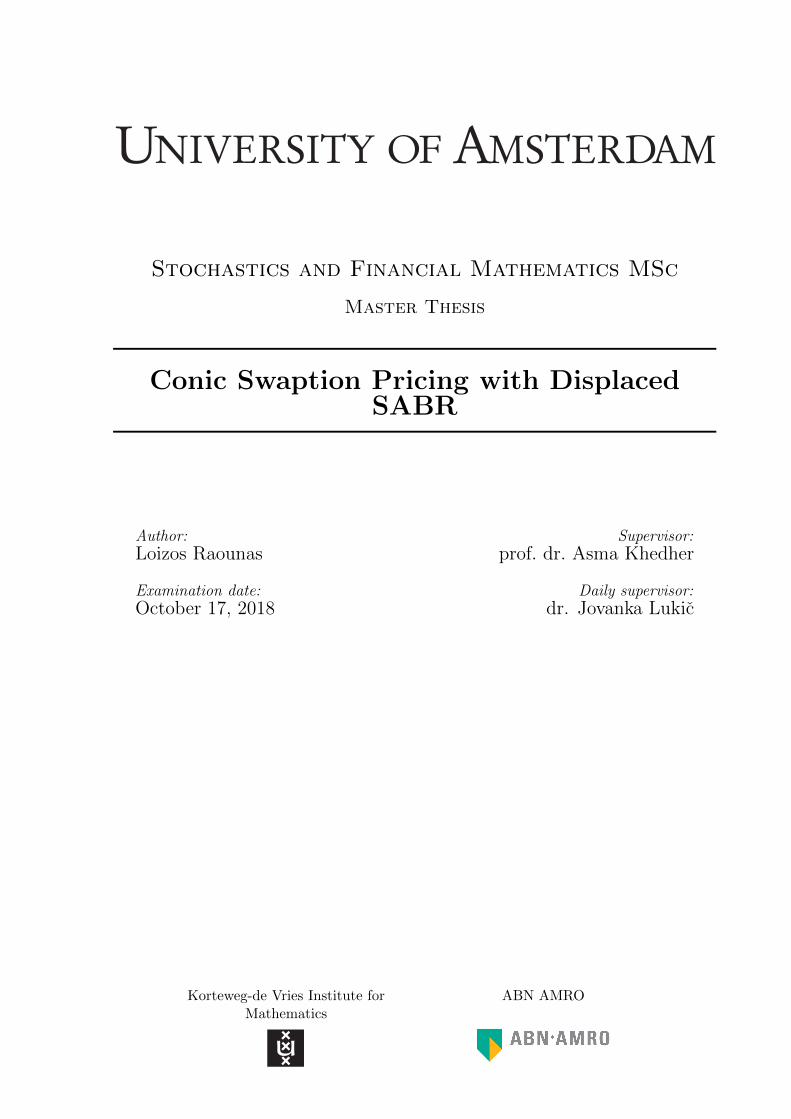
The following graph is a geometric representation of two-state conic binomial trees and risk-neutral probability p. We consider the asset to be in the up-state and the derivative to have apositive up-state payoff and zero down-state payoff (e.g. a European call option).
24
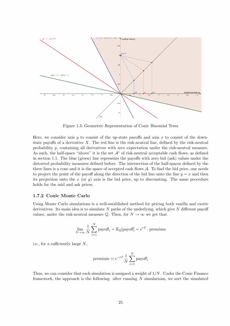
Figure 1.3: Geometric Representation of Conic Binomial Trees
Here, we consider axis y to consist of the up-state payoffs and axis x to consist of the down-state payoffs of a derivative X. The red line is the risk-neutral line, defined by the risk-neutralprobability p, containing all derivatives with zero expectation under the risk-neutral measure.As such, the half-space “above” it is the set A∗ of risk-neutral acceptable cash flows, as definedin section 1.1. The blue (green) line represents the payoffs with zero bid (ask) values under thedistorted probability measures defined before. The intersection of the half-spaces defined by thethree lines is a cone and it is the space of accepted cash flows A. To find the bid price, one needsto project the point of the payoff along the direction of the bid line unto the line y = x and thenits projection unto the x (or y) axis is the bid price, up to discounting. The same procedureholds for the mid and ask prices.
1.7.2 Conic Monte Carlo
Using Monte Carlo simulations is a well-established method for pricing both vanilla and exoticderivatives. Its main idea is to simulate N paths of the underlying, which give N different payoffvalues, under the risk-neutral measure Q. Then, for N →∞ we get that
limN→∞
1
N
N∑i=1
payoffi = EQ[payoff] = erT · premium
i.e., for a sufficiently large N ,
premium ' e−rT 1
N
N∑i=1
payoffi
Thus, we can consider that each simulation is assigned a weight of 1/N . Under the Conic Financeframework, the approach is the following: after running N simulations, we sort the simulated
25
payoffs in an ascending order, i.e.,
payoff(i) ≤ payoff(i+1), ∀i ∈ 1, . . . , N − 1.
It obviously holds that
e−rT1
N
N∑i=1
payoffi = e−rT1
N
N∑i=1
payoff(i).
Working under the Conic Finance framework, we assign higher weights to lower payoffs and lowerweights to higher payoffs to calculate the bid price and vice versa to calculate the ask price. Assuch, instead of assigning a uniform weight to all simulated payoffs, we use a distortion functionΨ to assign weights in the aforementioned manner to the sorted payoffs. Indeed, we use weightsp∗i for the bid price and pi for the ask price, given by:
p∗i = Ψ
(i
N
)−Ψ
(i− 1
N
), i ∈ 1, . . . , N
pi = Ψ
(N − i+ 1
N
)−Ψ
(N − iN
), i ∈ 1, . . . , N,
(1.19)
which we can compare to the “uniform” Monte Carlo weights as such: let a random variableX ∈ L∞(Ω,F ,P), a distortion function Ψ and an i.i.d.3 empirical sample x1, . . . , xN of X. Thenwe can estimate its expected value using the empirical distribution function, i.e.
E[X] '∫ +∞
−∞xdFX(x) =
N∑i=1
xi∆
(i
N
)=
1
N
N∑i=1
xi.
For its distorted expectation we thus have
DΨ[X] '∫ +∞
−∞xdΨ(FX(x)) =
N∑i=1
x(i)∆Ψ
(i
N
)=
N∑i=1
x(i)
(Ψ
(i
N
)−Ψ
(i− 1
N
)),
where we used x(i) instead of xi because of the different weights assigned through Ψ. Moreover,we see that (1.19) are indeed probability weights, as p∗i , pi ≥ 0 ∀i ∈ 1, . . . , N and
N∑i=1
p∗i =N∑i=1
pi = 1.
We also see that if Ψ is the identity function, then p∗i = pi ≡ 1/N , which is the probabilityweight assigned in the one-price framework. Thus, for N large enough, we have the following
3Independent and Identically Distributed.
26
equation for the bid price:
bid ' e−rTN∑i=1
p∗i payoff(i)
= e−rTN∑i=1
(Ψ
(i
N
)−Ψ
(i− 1
N
))payoff(i) (1.20)
while the corresponding equation for the ask price is given by:
ask ' e−rTN∑i=1
pipayoff(i)
= e−rTN∑i=1
(Ψ
(N − i+ 1
N
)−Ψ
(N − iN
))payoff(i) (1.21)
We also observe that the weights p∗i and pi only depend on the (pre-selected) distortion functionΨ and on the number of simulations N , but not on the simulated paths themselves. As such,the probability weights can be calculated either before or after the simulation procedure takesplace.
27
2 Swaptions and the SABR model
In this chapter we describe the model that has been utilized in this thesis, i.e. the (displaced)SABR model. We also give a description of the swaption, which is the financial product that weprice. Since swaptions are options having swaps as the underlying, we begin by giving a briefintroduction of swaps.
2.1 Swaps
A (vanilla) interest rate swap is an agreement between two parties: one party pays interest ata fixed rate on a notional for a predetermined time period, while receiving interest at a floatingrate on the same notional, for the same time period. The time period between the start of theswap and the last payment is called maturity. The floating rate is usually based on the LondonInterbank Offered Rate1 (LIBOR), which is the interest rate that London based banks withcredit rating AA charge in order to lend to each other (Hull [24]). An interest rate swap can befurther characterized depending on which party pays the fixed interest and which the floatinginterest. Indeed, from the point of view of the party that pays the fixed interest rate, the swapis called a payer swap, while for the party paying the floating interest rate, it is called a receiverswap. In the following, we describe how the cash flows associated with swaps were tradition-ally calculated, using a Single Curve framework and how this has changed into a Multi-Curveframework after the 2008 financial crisis.
2.1.1 Single Curve Framework
In the following, we follow Filipovic [16]. Consider that there are n payments taking place atdates T0 < T1 < . . . < Tn, with Ti − Ti−1 ≡ δ. We denote N to be the notional and K the fixedinterest rate. Then the value of the fixed interest payments (“fixed leg”) can be calculated asthe sum of the discounted cash flows, i.e.:
pfix(t) = NKδn∑i=1
P (t, Ti) +NP (t, Tn), t ≤ T1
where by P (t, T ) we denote the zero coupon bond at time t, with maturity T , which representsthe discounting. The NP (t, Tn) part of the right hand side represents the return of the (dis-counted) notional during the last payment at Tn. The value of the floating interest payments(“floating leg”) can be calculated as the sum of the discounted cash flows:
pfloat(t) = Nδ
n∑i=1
P (t, Ti)F (Ti−1, Ti) +NP (t, Tn), t ≤ T0,
1Depending on the currency, there are other IBORs used, such as EURIBOR for the euro.
28
where the fixed rate K has been replaced with F (Ti−1, Ti), which is an interest rate for the timeinterval [Ti−1, Ti), fixed at Ti−1. Note that here we have assumed for simplicity that the numberof cash flows for the fixed and the floating leg is the same, hence δfix = δfloat = δ, but this is notnecessarily the case. Thus, the value of a payer swap at time t ≤ T0 is Πp(t) = pfloat(t)− pfix(t),which can be calculated (Filipovic [16]) to be:
Πp(t) = N
(P (t, T0)− P (t, Tn)−Kδ
n∑i=0
P (t, Ti)
).
For the receiver swap, we need only change the sign of the cash flows, thus getting
Πr(t) = −Πp(t).
Hence, we are now able to calculate the “fair” value of the fixed rate, i.e. the value of K suchthat Πp(t) = Πr(t) = 0. For t = 0, we call this the swap rate and denote it as Rswap(0), whichis calculated to be
Rswap(0) =P (0, T0)− P (0, Tn)
δ∑n
i=1 P (0, Ti),
hence at time t ≤ T0, we have
Rswap(t) =P (t, T0)− P (t, Tn)
δ∑n
i=1 P (t, Ti).
As can be seen, the swap rate is calculated using only one interest rate curve. Additionally, wemay compute the forward swap rate for any time before the first payment 0 < t ≤ T0:
Rfwdswap(t)∣∣∣t=0
= E[Rswap(t)
∣∣F0
]= E
[P (t, T0)− P (t, Tn)
δ∑n
i=1 P (t, Ti)
∣∣∣∣F0
].
2.1.2 Multi-Curve Framework
Traditionally, LIBOR was considered to entail insignificant risk and as such was used as a proxyfor the risk-free interest rate (Hull and White [23]). Hence, LIBOR was used for both definingthe floating interest rate and for discounting, leading to the Single Curve framework discussedbefore. However, the events of the financial crisis of 2008, showed that this was not the caseand led to a different approach. Namely, the Overnight Index Swap2 (OIS) rate has becomeincreasingly popular as a risk-free rate proxy. The reason for this is that, because OIS allowsthe interbank loans to be rolled into the next day, it entails less risk than LIBOR. As such,it is becoming more and more common to use OIS as the discount rate (Henrard [21]). Formore details on OIS and the events leading it gradually replacing LIBOR for the purpose ofdiscounting, we refer to [21] and [23].Under this framework, we denote by D(t, T ) the discounting derived from the OIS curve and byF (Ti−1, Ti) the interest rate of the time interval from Ti−1 to Ti, derived from the forward curve
2“An OIS is a swap where a fixed rate for a period is exchanged for the geometric average of the overnight ratesduring the period” (Hull [24]).
29
(LIBOR or otherwise). We now examine the more general case where, for the fixed leg we havem payments and consider T fix
j − T fixj−1 ≡ δfix for every j ∈ 1, . . . ,m. Correspondingly, for the
floating leg we consider n payments and T floati − T float
i−1 ≡ δfloat for every i ∈ 1, . . . , n. Then,we calculate the swap rate at t = 0 to be
Rswap(0) =δfloat
∑ni=1 F (Ti−1, Ti)D(0, Ti)
δfix∑m
j=1D(0, Tj)(2.1)
and at t ≤ T1 we have:
Rswap(0) =δfloat
∑ni=1 F (Ti−1, Ti)D(0, Ti)
δfix∑m
j=1D(0, Tj). (2.2)
Hence, the forward swap rate is calculated to be
Rfwdswap(t)∣∣∣t=0
= E[Rswap(t)
∣∣F0
]=δfloat
δfixE
[∑ni=1 F (Ti−1, Ti)D(t, Ti)∑m
j=1D(t, Tj)
∣∣∣∣F0
]. (2.3)
2.2 Swaptions
Swaptions are derivatives whose underlying is an interest rate swap. They give the holder theright (but not the obligation) to enter a swap at a predetermined swap rate, at a predeterminedfuture date (Hull [24]). They are defined by three dates: the date in which the swaptionis issued, called start date, the date in which the holder of the swaption decides whether toexercise the option or not, called the expiry date and the date describing how long the swappayments last after the option is exercised, called the maturity date. There are two main typesof swaptions: the “swap-settled” swaptions, in which exercising the swaption leads to enteringthe underlying swap and the “cash-settled” swaptions, in which exercising the swaption leadsto a cash settlement upon the expiry date (Pietersz and Sengers [35]). Swap-settled swaptionsare popular when USD is the currency, while cash-settled swaptions are popular when EURor GBP is the currency [35]. Following Mercurio [33] and applying the Multi Curve frameworkdiscussed in the previous section with t0 < T < T1 < . . . < Tn = τ , the payoff of the swap-settledswaptions at t = T is:
payoffswap = N ·AswapT · (ω · (ST −K))+
where
AswapT =
n∑i=1
δiD(T, Ti) (2.4)
and we define
Aswapt := D(t, T )AswapT .
30
The payoff of the cash-settled swaptions at t = T is:
payoffcash = N ·AcashT · (ω · (ST −K))+ (2.5)
where
AcashT =
n∑i=1
1m(
1 + 1mR(T )
∣∣t
)i . (2.6)
Again, we define
Acasht := D(t, T )AcashT
In the previous formulas, we have used the following notation:
• t0: start date
• T : expiry date of the swaption
• τ : the maturity date of the swaption
• D(t1, t2): discounting factor from t1 to t2, based on the discounting curve
• n: number of floating payments of the underlying swap
• m: number of fixed leg payments per annum
• δi: year fraction corresponding to the i-th fixed leg payment
• R(T )∣∣t=t0
: the forward swap rate for expiry T and tenor τ , at t0, as described in (2.3)
• ST : the value of the underlying swap at time t = T
• K: the strike of the option
• N : the notional of the underlying swap
• ω: ω = 1 if it is a payer swap, ω = −1 if it is a receiver swap
We call (2.4) the swap annuity, or present value of a basis point (PVBP). The equivalent martin-gale measure Qswap using (2.4) as the numeraire, is called the (swap-settled) annuity measure,under which payoffswap is a martingale (Henrard [21]). Hence, using the same notation as before,the premium of a swap-settled swaption is given by:
Vswap(t) = NAswapt EQswap[(ω(ST −K))+
∣∣Ft] (2.7)
or, through (2.4):
Vswap(t) = ND(t, T )
n∑i=1
δiD(T, Ti)EQswap[(ω(ST −K))+
∣∣Ft] .
31
Correspondingly, we call (2.6) the cash annuity and the premium of a cash-settled swaption isgiven by:
Vcash(t) = D(t, T )EQT[payoffcash
∣∣Ft]where QT is the T -forward measure. In the swap-settled swaption case, the swap annuity isessentially a portfolio of zero-coupon bonds and as such may conveniently be used as a numeraire.However, the cash-settled annuity is merely an auxiliary quantity and thus has no representationas a financial product, therefore it cannot be used as a numeraire. Hence, to calculate thepremium, we make the assumption that the cash-settled swaption is a martingale under theannuity measure, hence:
Vcash(t)
Aswapt
= EQswap[
payoffcashAswapT
∣∣∣∣∣Ft]
or
Vcash(t) = NAswapt EQswap[AcashT
AswapT
(ω(ST −K))+
∣∣∣∣∣Ft]. (2.8)
While the Single-Curve framework was the standing market practice, Acasht was considered asan approximation of Aswapt , hence AswapT ' AcashT , making (2.8):
Vcash(t) = NAcasht EQswap[(ω(ST −K))+
∣∣Ft] (2.9)
or
Vcash(t) = ND(t, T )n∑i=1
1m(
1 + 1mR(T )|t
)iEQswap [(ω(ST −K))+∣∣Ft] . (2.10)
This is a mathematically wrong result, since the cash-settled swaption premium is not a mar-tingale under the swap-settled measure. However, under the Single Curve framework, the er-rors of this approach were considered small enough to justify its use. Under the Multi-Curveframework, these errors have become non-insignificant and have led to quoting different impliedvolatilities for swap/cash settled swaptions, quoting different premiums for ATM payer and re-ceiver cash settled swaptions, as well as quoting non-negligible prices for cash-settled zero-widthcollars3 (Pietersz and Sengers [35]). However, (2.9) is still the “the market-standard formulafor cash-settled swaptions” [35] and as such we consider (2.10) as our starting point for pricingcash-settled swaptions.
3A zero-width collar is buying a payer swaption and selling a receiver swaption with the same strikes. Its valuefor cash-settled swaptions not being zero, implies that put-call parity does not hold.
32
2.3 SABR
In this section, we describe the SABR model, which was introduced by Hagan et al. [19] andunless otherwise stated, we follow their original work.
2.3.1 Original SABR Model
The SABR model is a stochastic volatility model given by the equations:
dFt = σtFβt dW
(1)t , F0 = f
dσt = νσtdW(2)t , σ0 = α
(2.11)
where Ft represents the forward value of the underlying, σt the volatility, ν is the volatility ofthe volatility (or “volvol”) and for the parameters it holds that 0 ≤ β ≤ 1, ν > 0. Furthermore,we assume that the two Brownian motions are correlated:
dW(1)t dW
(2)t = ρdt, −1 ≤ ρ ≤ 1. (2.12)
We also impose the boundary condition that F = 0 is absorbing. In our swaption pricing case,we consider f = Rfwdswap(T )
∣∣t=0
as defined in (2.3), with T being the expiry date of the swaption.The name of the model itself is derived from its parameters: SABR is an acronym for StochasticAlpha Beta Rho. It is worth mentioning that the second equation of (2.11) can be solvedanalytically. Indeed, by applying Ito’s lemma for f(x) = log x, we get
σt = σ0 exp
(−1
2ν2t+ νW
(2)t
). (2.13)
Moreover, for the special cases in which β = 0 or β = 1, then both equations of (2.11) havean explicit solution, with the underlying having a normal distribution in the β = 0 case and alog-normal distribution in the β = 1 case.
SABR was developed trying to solve the weaknesses of its contemporary standard market mod-els. Namely, on one hand, the celebrated Black’s [5] model which, even though dominant in themarket, made the rather strong assumption that the volatility remains constant. Since we haveample historical data of markets being (relatively) stable in some periods and outward chaoticin other periods, considering the volatility to be constant is unrealistic.
To deal with this problem, “local volatility” models were developed, in which the volatilitywas considered to be dynamic. In the work of e.g. Dupire [14], the proposed model was:
dFt = σloc(t, Ft)FtdWt, F0 = f
under the forward measure, with σloc(t, Ft)Ft being Markovian. Then, the local volatility wasobtained by calibrating the model to market values of liquid derivatives. The problem with thisapproach is that it captures the wrong dynamics of the implied volatility curve [19], i.e. for anincrease of the underlying price it predicts that the implied volatility curve shifts to lower pricesand vice versa, which is contradictory to the real market behavior.
33

Thus, building on the idea that volatility should not be considered constant, (2.11) and (2.12)were used to define the SABR model, which captures the correct dynamics. Another advantageof SABR is that by using singular perturbation techniques, an analytic formula for the impliedvolatility can be calculated. Indeed, for not ATM strikes, i.e. when K 6= f we have the formula:
σIMP (K, f) =α
(fK)(1−β)/2[1 + (1−β)2
24 log2(fK
)+ (1−β)4
1920 log4(fK
)+ . . .
] · ( z
χ(z)
)·
·(
1 +
[(1− β)2
24
α2
(fK)(1−β)+
1
4
αβρν
(fK)(1−β)/2+
2− 3ρ2
24ν2
]+ . . .
) (2.14)
with
z =ν
σ(fK)(1−β)/2 log
(f
K
)and
χ(z) = log
(√1− 2ρz + z2 + z − ρ
1− ρ
).
When K = f , (2.14) reduces to:
σIMPATM = σIMP (f, f) =
α
f (1−β)
(1 +
[(1− β)2
24
α2
f2−2β+
1
4
αβρν
f (1−β)+
2− 3ρ2
24ν2
]T + . . . (2.15)
The extra terms in (2.14) and (2.15) are omitted because they are much smaller than the firstterms. For more details on the derivation of (2.14) and (2.15), we refer to the original paper byHagan et al. [19]. The implied volatility calculated by these formulas can then be used as inputto Black’s formula, to obtain the premium’s value.
The parameters β and ρ affect the σIMP (K) curve in a similar way, which is why it is standardpractice to fix a constant value for β a priori and then, for fixed expiry and maturity dates, cali-brate the rest of the parameters to fit a curve σIMP
MKT (K) of market observed implied volatilities.A way to do this is by least-square minimizing, that is, as seen e.g. in Rouah, F. D. [36]:
(α, ρ, ν) = arg minα,ρ,ν
∑i:Ki
(σIMPMKT (Ki)− σIMP (Ki, f ;α, ρ, ν)
)2, (2.16)
with i ranging through the available strikes Ki of the fixed expiry and maturity. Then weplug the derived α, ρ, ν values into (2.14) and (2.15) to calculate the implied volatilities for allthe strike values of the fixed expiry and maturity date. Another common practice is to firstcalculate α through the ATM equation (2.15), using the value for the ATM implied volatilityand calibrating with respect to ρ and ν. Then, given the known α and β, ρ and ν are calibrated
34
as before. Again following [36], we may write this procedure as:
(α, ρ, ν) = arg minα,ρ,ν
∑i:Ki
(σIMPMKT (Ki)− σIMP (Ki, f ;α(ρ, ν), ρ, ν)
)2(2.17)
In the σIMP (K) curve, the role of the parameters is as such: α controls the overall height of thecurve, ν controls how much “smile” the curve has and ρ controls the curve’s skew.
2.3.2 Negative Interest Rates SABR adaptations
Because of the F βt term in (2.11) and the fact that 0 ≤ β ≤ 1, Ft is not allowed to have negativevalues, except when β = 0 or β = 1. In the swaption pricing case, this property had the intuitiveexplanation that interest rates could never be negative, hence this property of SABR was consid-ered an advantage. However, in the current post-crisis, low interest rate environment, negativeinterest rates are a reality and so SABR needed to be extended in a way that allows negativeinterest rates as well, that is to allow Ft < 0. Two such extensions are the “Free Boundary”SABR and the “Displaced” (or “Shifted”) SABR.
Free Boundary SABRIn the Free Boundary SABR, the absorbing boundary condition is dropped and (2.11) is modifiedto:
dFt = σt|Ft|βdW (1)t
dσt = νσtdW(2)t
with (2.12) remaining the same. Hence, since |Ft|≮ 0, ∀t ≥ 0, Ft is allowed to have negativevalues. For more information on the Free Boundary SABR, see Antonov et al. [2].
Displaced SABROn the other hand, the Displaced (or Shifted) SABR, whose use we employ in this thesis, dealswith the possible negative values of Ft by introducing a deterministic (potentially non-constant)displacement factor d > 0 such that F ′t := Ft + d. The displacement factor needs to be largeenough to “absorb” all foreseeable negative interest rates, i.e. F ′t ≥ 0, for every t in the timehorizon. Thus, we replace Ft with F ′t in (2.11), getting:
dF ′t = σtF′tβdW
(1)t
dσt = νσtdW(2)t
(2.18)
with (2.12) remaining again unaltered. An advantage of this approach is that, given the originalSABR setting, all that is needed to extend to the displaced SABR is a minor modification.Indeed, if we define the displaced strike as K ′ := K + d and take the displaced underlying F ′tdefined as before, we see that:
E[(Ft −K)+] = E[((Ft + d)− (K + d))+] = E[(F ′t −K ′)+]
35
under any probability measure. Hence, pricing a derivative under the original or the DisplacedSABR is the same, if we displace both the underlying and the strike. Also, (2.14) becomes
σIMP (K ′, f ′) =α
(f ′K ′)(1−β)/2[1 + (1−β)2
24 log2(f ′
K′
)+ (1−β)4
1920 log4(f ′
K′
)+ . . .
] · ( z′
χ(z′)
)·
·(
1 +
[(1− β)2
24
α2
(f ′K ′)(1−β)+
1
4
αβρν
(f ′K ′)(1−β)/2+
2− 3ρ2
24ν2
]+ . . .
)(2.19)
with
z′ =ν
σ(f ′K ′)(1−β)/2 log
(f ′
K ′
)and
χ(z) = log
(√1− 2ρz + z2 + z − ρ
1− ρ
)
while (2.15) becomes
σIMPATM = σIMP (f ′, f ′) =
α
f ′(1−β)
(1 +
[(1− β)2
24
α2
f ′2−2β+
1
4
αβρν
f ′(1−β)+
2− 3ρ2
24ν2
]T + . . . (2.20)
A disadvantage of this approach is that the displacement factor cannot be directly observed fromthe market. Its value can be determined indirectly from the market, by observing the impliedvolatilities curve extracted by the market premiums. It can also be determined by consideringthe displacement factor as an extra SABR parameter for calibration/curve fitting. For moredetails on the displaced SABR, see Hagan & Kumar [20].
36
3 Methodology
We now present the data we have used and the methodology that we have followed.
3.1 Data
The data used in testing consisted of two sets, one for swap-settled and one for cash-settledswaptions. Each data set contained the (undiscounted) market quoted premiums of swaptionswith several expiry/tenor dates, for multiple strike values. Each set also contained a 3 monthinterest rate curve, a 6 month interest rate curve and an OIS interest rate curve for multiplefuture dates, in their respective currency (USD for swap-settled, EUR for cash-settled). Bothwere retrieved from ICAP and had 31/10/2017 as their start date.
3.1.1 Cash Settled (EUR)
For the cash-settled case, the quoted market premiums expiries and maturities belong in theset 1, 2, 5, 10, 15, 20, 30 (in years), with each swaption being a combination of two of thesenumbers denoted as “XyZy”. Hence, e.g., in the following, the “2y5y” swaption corresponds tothe swaption with expiry date 2 years after the starting date and swap maturity 5 years after theswaption expiry date. The interest rate curves (3m/6m/OIS) each consist of 45 values rangingfrom 1 day after the starting date to 60 years after the starting date, thus containing valuesfor the entire time horizon, up to the furthest date of the 30y30y swaption. Since we used themarket practice of considering the “spot date1” for the expiry/maturity dates, we applied linearinterpolation to calculate interest rates of dates not available in our interest rate curve data.The payment frequencies are: once per year for the fixed leg, while for the floating leg every 3months if the swap maturity is 1 year and every 6 months otherwise.Then, for a swaption with fixed expiry and maturity dates, there is a premium correspondingto each strike value. The strike values K are expressed as the distance from the ATM swap rate(2.3), measured in basis points2(“bp”) i.e.
K = Rfwdswap(T )∣∣t=0
+ bp
The available strikes are for 0, ±6.25, ±12.5, ±25, ±50, ±75, ±100, ±150, ±200 and ±300 basispoints, with the bp = 0 case clearly being the ATM strike. In our analysis, we ignored all ±300bpswaptions, as well as swaptions with a zero quoted premium. The premiums corresponding topositive basis points belong to payer swaptions, while those of negative basis points belong toreceiver swaptions. Hence, from (2.5) we see that all non-ATM swaptions examined here areOut-of-The-Money (“OTM”). The ATM premium is quoted as the sum of a payers ATM anda receivers ATM swaption. However, as discussed in Section 2.2, the payer and receiver cash-settled (EUR) ATM premiums have a non-negligible spread. Hence, we used zero-width collar
1Two business days after the actual date.21 basis point = 10−4.
37
quotes from ICAP in order to derive the unequal payer and receiver ATM premiums.Lastly, a displacement factor is given for swaptions with maturities of 1, 5, 10, 20 and 30years; for maturities of 2 and 15 years, we calculate the displacement factor by using linearinterpolation.
3.1.2 Swap Settled (USD)
The data given for the swap-settled swaptions were equivalent to the cash-settled swaptions,with the following exceptions. First, the expiry dates belong in the set 1, 2, 5, 10, 15, 20 (no30 years expiries available). Then, the spread between payer and receiver ATM is considered tobe negligible, hence the quoted ATM premium is calculated as the sum of the ATM payers andATM receivers premium. Also, the strikes quoted are for the basis points 0, ±6.25, ±12.5, ±25,±37.5, ±50, ±75, ±100, ±150, ±200 and ±300 (±37.5 is included, unlike with the cash-settledswaptions). However, the quoted premium for all -300bp and almost all +300bp swaptions was0, so we omitted all ±300bp swaptions from our analysis. The payment frequencies are: every 3months for the floating leg and every 6 months for the fixed leg. Lastly, the displacement factoris identical for all maturity dates.
3.2 Calibration
For the calibration of the SABR parameters α, β, ν, ρ, we proceeded with two different ap-proaches, one deterministic and one stochastic. In both approaches, we take β = 0.5 andcalibrate the parameters for fixed expiry/maturity dates.
Deterministic ApproachIn the first approach, we solved (2.20) with respect to α, by picking two arbitrary values for ρand ν (e.g. ρ = 0.5 and ν = 0.3) and taking
σIMPATM =
2√T
N−1
[1
2
(V∗(0)
D(0, T )N A∗T+ 1
)](3.1)
i.e. the solution of Black’s formula for swaptions with respect to the implied volatility, for theATM case. Here we use the notation of Chapter 2, with N−1 being the inverse of the standardnormal cumulative distribution and ∗ ∈ swap, cash. Then, we get ρ and ν through (2.17). Aproblem with this approach is that it does not guarantee that the minimum it finds is in factthe global minimum. Hence, a poor choice of initial conditions might lead to a local, insteadof the global, minimum. A way to improve the local minimum in our case, is to apply thealgorithm once using arbitrary values for ρ, ν and then use the algorithm’s resulting ρ′, ν ′ valuesas the initial condition of a new algorithm application. This obviously makes this method moretime consuming, but leads to solving the problem of a potentially bad choice of initial conditions.
Stochastic ApproachOur second approach was using the Differential Evolution (DE) algorithm, which is a stochas-tic, global optimization algorithm developed by Storn & Price [37]. In it, the objective functionf : X ⊆ RD → R with X 6= ∅, where D is the number of parameters to be optimized, does nothave to be differentiable, continuous or linear. Differential Evolution allowed us to calibrate allSABR parameters (α, ρ, ν) simultaneously, without the need of providing initial conditions. The
38
version of DE that we have applied is DE/best/1/bin, of which we give a brief description.
First, we provide a population number NP ≥ 4, i.e. the number of RD vectors that willbe used for the optimization procedure, upper and lower boundaries xU ,xL ∈ RD to definethe space X , a “crossover constant” CR ∈ [0, 1] and a termination criterion (either a tolerancelevel or a maximum number of “generations”). Unless specified otherwise, whenever we makea random decision, a uniform distribution is assumed. The initial vectors are chosen randomlyfrom the entire X . Hence, we have
xL ≤ xi,0 ≤ xU
where xi,0 ∈ RD, for every i ∈ 1, . . . , NP. We denote the vectors of generation G ∈ N as xi,G.We call these vectors “agents”. Given that we are in generation G, the steps of the algorithmare as such:
1. Mutation: For each agent xi,G, i ∈ 1, . . . , NP, randomly choose two indices r1,G, r2,G ∈1, . . . , NP, such that xr1,G 6= xr2,G , xr1,G 6= xi,G and xr2,G 6= xi,G. Then, assign
vi,G+1 := g + F · (xr1,G − xr2,G)
where F ∈ [0, 2] is a constant factor and g = (g1, . . . , gD) is the agent correspondingto the best position in X until this point, i.e. f(g) ≤ f(xi,k) ∀i ∈ 1, . . . NP and∀k ∈ 1, . . . , G. We call vi,G+1 = (v1i,G, . . . , vDi,G) ∈ RD “mutant vectors”.
2. Crossover: Now, for every i ∈ 1, . . . , NP we introduce a trial vector ui,G+1 = (uji,G+1)j ,j ∈ 1, . . . , D as such:
uji,G+1 =
vji,G+1 if rndb(j) ≤ CR or j = Ri
xji,G if rndb(j) > CR and j 6= Ri
where rndb(j) ∼ Unif[0, 1], drawn separately for each j ∈ 1, . . . , D and Ri is an indexchosen randomly from 1, . . . , D. This ensures that every trial vector contains at leastone value from its respective mutant agent.
3. Selection: Finally, to decide which agents will be used in generation G + 1, we have forevery i ∈ 1, . . . , NP:
xi,G+1 =
ui,G+1 if f(ui,G+1) ≤ f(xi,G)
xi,G otherwise
Steps 1 to 3 are then repeated until a termination criterion is reached. For more on DE and itsother versions, we refer to Fulcher [18] and Pedersen [34].
3.3 Simulation
We now describe the methods we have used in order to simulate the value of the underlyingat the expiry of the swaption, i.e. ST . These simulations were run multiple times, in order to
39
approximate E[(ω(ST −K)+] through Monte Carlo.
3.3.1 Euler Scheme
We start by considering a time horizon [0, T ] and dividing it into N time steps ti, where t0 = 0,tN = T and ti+1 − ti ≡ ∆t, for every i = 0, . . . N − 1, i.e. ∆t = 1/N . Hence, the discretizedversion of (2.18)
dF ′t = σtF′tβdW
(1)t
dσt = νσtdW(2)t
may be written as:
F ′ti+1= σtiF
′tiβ(W
(1)ti+1−W (1)
ti) + F ′ti
σti+1 = νσti(W(2)ti+1−W (2)
ti) + σti
(3.2)
and since for a Brownian Motion W it holds that W (t) −W (s) ∼ N(0, t − s), we can rewrite(3.2) as
F ′ti+1= σtiF
′tiβε(1)√
∆t+ F ′ti
σti+1 = νσtiε(2)√
∆t+ σti(3.3)
with ε(1) ∼ N(0, 1) and ε(2) ∼ N(0, 1), correlated under (2.12), where N(0, 1) is the standardnormal distribution.
Continuing, we apply the Cholesky decomposition to (2.12), giving us:
dW(1)t = ρdWt +
√1− ρ2dZt
dW(2)t = dWt
where W and Z are independent standard Brownian Motions. Hence, (3.3) becomes
F ′ti+1= σtiF
′tiβ(ε1ρ+ ε2
√1− ρ2
)√∆t+ F ′ti
σti+1 = νσtiε1√
∆t+ σti
(3.4)
where ε1 and ε2 are independent random variables with ε1 ∼ N(0, 1) and ε2 ∼ N(0, 1). Fur-thermore, we take initial conditions F ′0 = E
[Rswap(T )
∣∣F0
]+ d (see (2.3)) with T being the
swaption’s expiry date and d the appropriate displacement factor and σ0 = α, derived from thecurve fitting procedure discussed before.
Remark 3.1. For the Euler scheme to have a guaranteed rate of strong or weak convergence(for a definition of strong and weak convergence see e.g. [25]), we need that the coefficients of(2.11) are globally Lipschitz continuous [28]. Hence, for the SABR, the classical Euler schemehas no theoretical result for a guaranteed convergence. However, we use it because of its wide
40
application in mathematical finance.
3.3.2 Semi-Exact
Our second simulation method is based on the 2017 paper by Cai, Song and Chen [7]. Their
approach focuses on directly simulating the conditional expectation of FT given σ0, σT ,∫ T
0 σ2sds
and F0, instead of simulating the entire path in order to reach its terminal value at T . By doingso, the inherent bias of time discretization techniques, as in the case of the Euler or Milsteinscheme is avoided. Cai et al. [7] present an exact simulation for two special cases and providea “semi-exact” simulation for the general case. We present the final results of the conditionaldistribution of FT and then, for the general case, we describe their approach to simulate the“intermediate” distributions of σT and
∫ T0 σ2
sds, needed for the simulation of the conditional dis-tribution of FT . Before doing so, we first present some special functions that are used afterwards.
Special FunctionsA non-central chi-squared random variable χ′2(µ;λ) with µ degrees of freedom and noncentralityparameter λ has probability density function
qχ′2(x;µ, λ) =1
2exp
(−x+ λ
2
)(xλ
)µ−24Iµ−2
2(√λx)
where Ia(·) is the modified Bessel function of the first kind with index a given by
Ia(x) =∞∑k=0
(x/2)a+2k
k!Γ(a+ k + 1)
where Γ(·) is the gamma function Γ(x) =∫∞
0 tx−1e−tdt, with x > 0 and a > −1. If λ = 0,then we have the special case of the central chi-squared random variable χ2(µ) with µ degreesof freedom and probability density function
qχ2(x;µ) =e−x/2xµ/2−1
2µ/2Γ(µ/2)
We denote their cumulative distribution functions by Qχ′2(x;µ, λ) and Qχ2(x;µ) respectively.Let us now present the results for the conditional distribution of FT . The following propositioncan be found in Islah [26].
Proposition 3.2. Fix T > 0 and suppose that σ0, σT ,∫ T
0 σ2sds and F0 are given.
(1) Let β = 1. Then, Ft is log-normally distributed and through (2.13), we have that
logFt ∼ N(
logF0 −1
2
∫ T
0σ2sds+
ρ
ν(σT − σ0), (1− ρ2)
∫ T
0σ2sds
)
41
(2) Let 0 ≤ β < 1, ρ = 0 and assume that Ft has an absorbing boundary at 0. Then:
P[FT = 0
∣∣∣∣F0, σ0, σT ,
∫ T
0σ2sds
]= 1−Qχ2
(A0;
1
1− β
)and
P[FT ≤ u
∣∣∣∣F0, σ0, σT ,
∫ T
0σ2sds
]= 1−Qχ′2
(A0;
1
1− β,C0(u)
), u > 0
where
A0 =1∫ T
0 σ2sds
(F 1−β
0
1− β
)2
and C0(u) =1∫ T
0 σ2sds· u
2(1−β)
(1− β)2
(3) Let ρ 6= 0, 0 ≤ β < 1 and assume that Ft has an absorbing boundary at 0. Then:
P[FT = 0
∣∣∣∣F0, σ0, σT ,
∫ T
0σ2sds
]= 1−Qχ2
(A; 1 +
β
(1− β)(1− ρ2)
)(3.5)
and
P[FT ≤ u
∣∣∣∣F0, σ0, σT ,
∫ T
0σ2sds
]= 1−Qχ′2
(A; 1 +
β
(1− β)(1− ρ2), C(u)
), u > 0 (3.6)
where
A =1
(1− ρ2)∫ T
0 σ2sds
(F 1−β
0
1− β+ρ
ν(σT − σ0)
)2
(3.7)
and
C(u) =1
(1− ρ2)∫ T
0 σ2sds· u
2(1−β)
(1− β)2. (3.8)
In our setting, we have calculated values for σ0 and F0, hence we only need to simulate values forσT (straightforward through (2.13)) and
∫ T0 σ2
sds. Thus we focus on the simulation of∫ T
0 σ2sds,
given σ0 and σT . Cai et al. [7] used results from Yor [38] to show the following.
Proposition 3.3. The density function of∫ T
0 σ2sds, conditioning on σ0 and σT is given by
P
[∫ T
0σ2sds ∈ dw
∣∣∣∣∣σ0, σT
]=ν√
2πT
wexp
1
2ν2
(1
T
[ln
(σTσ0
)]2
−σ2T + σ2
0
w
)·
·I0(r)fr(ν2T )dw
42
where Ia(·) is the modified Bessel function of the first kind with index a, r ≡ r(w) = σ0σT /(ν2w)
and fr(·) with r > 0 is the Hartman-Watson density function:
fr(t) =1
I0(r)
r√2π3t
exp
(π2
2t
)·
·∫ ∞
0exp
(−y
2
2t
)exp
(− r cosh(y)
)sinh(y) sin
(πyt
)dy, t > 0.
Even though (3.3) provides an explicit expression for∫ T
0 σ2sds, the Hartman-Watson density
function is “extremely difficult to compute for small t” [7], because the term outside the integral
(r/√
2π3t)·exp(π2/2t
) t→0−→∞ exponentially, while the term sin(πy/t) inside the integral changesits sign more and more frequently as t → 0. To achieve acceptable results, high-precisioncomputations are required, something that is not always computationally feasible. To tacklethis problem, Cai et al.[7] employed the following approach: instead of numerically calculatingthe conditional distribution directly, they used an appropriate bijection h : R+ → R+, such thatthe Laplace transform of the cumulative distribution function of h(
∫ T0 σ2
sds), given σ0 and σT
has a closed form. We denote the cumulative distribution function of h(∫ T
0 σ2sds) given σ0 and
σT as Lh(·) and its Laplace transform as Lh(·) with
Lh(θ) :=
∫ ∞0
e−θuLh(u)du, θ > 0
Then, we have the following proposition.
Proposition 3.4. For h(x) = 1/x, the Laplace transform of Lh(·) is:
Lh(θ) =1
θexp
−
[φln(σT /σ0)(θν2/σ2
0)]2 − [ln(σT /σ0)]2
2ν2T
with
φx(λ) = arcosh(λe−x + cosh(x)),
where cosh(y) = (ey + e−y)/2 and arcosh(z) = (ln(z +√z2 + 1).
We thus see that choosing h(x) = 1/x leads to a Laplace transform that consists only of relativelysimple functions. Continuing, applying the Euler inversion algorithm by Abate and Whitt [1],we may calculate Lh(·) from Lh(·) by
Lh(u) =eM/2
2uRe
(Lh
(M
2u
))+eM/2
u
∞∑k=1
(−1)kRe
(Lh
(M − 2kπi
2u
))− ed, (3.9)
where Re(x) is the real part of x, i is the imaginary unit i =√−1, M is a positive constant and
43
ed is the discretization error
ed = ed(Lh, u,M) =
∞∑k=1
e−kMLh((2k + 1)u
).
Since Lh(·) is a cumulative distribution function, it is non-decreasing and 0 ≤ Lh(·) ≤ 1. Hence,if Lh(·) ≡ 0 we have ed = 0, while if Lh(·) ≡ 1, then
ed =∞∑k=1
e−kM =1
eM − 1=
e−M
1− e−M
Hence, we can bound ed
0 ≤ ed ≤e−M
1− e−M' e−M (3.10)
for sufficiently large M . Additionally, we approximate the alternating power series of (3.9) byusing the Euler transformation
∞∑k=0
(−1)kak ' E(m,n) :=m∑k=0
m!
k!(m− k)!2−mSn+k (3.11)
with
Sj :=
j∑k=0
(−1)kak.
In our implementation, we follow the paper’s suggestion and take M = 20, m = 20 and n = 35.Hence, (3.9) using the approximations (3.10) and (3.11) becomes:
Lh(u) =eM/2
2uRe
(Lh
(M
2u
))
+eM/2
u
m∑k=0
m!
k!(m− k)!2−m
n+k∑j=0
(−1)jRe
(Lh
(M − 2jπi
2u
))− e
M/2
uRe
(Lh
(M
2u
))− e−M .
(3.12)
Thus, through (3.12) we have a computationally efficient formula for the cumulative distribution
function of h(∫ T
0 σ2sds) = 1/
∫ T0 σ2
sds given σ0, σT . Hence, to sample∫ T
0 σ2sds given σ0, σT , we
work as such: we simulate U ∼ Unif[0, 1] and solve Lh(V ) = U numerically using some root
44
finder algorithm. Then, V has the same distribution as 1/∫ T
0 σ2sds given σ0, σT , so
1/V ∼∫ T
0σ2sds given σ0, σT .
We are now ready to simulate the distribution of FT given F0, σ0, σT ,∫ T
0 σ2sds, using (3.5) and
(3.6). To do so, we work as before and simulate U ∼ Unif[0, 1]. Then, if
U ≤ P[FT = 0
∣∣∣∣F0, σ0, σT ,
∫ T
0σ2sds
]= 1−Qχ2
(A; 1 +
β
(1− β)(1− ρ2)
)we set FT = 0. Otherwise, we numerically solve
U = P[FT ≤ V
∣∣∣∣F0, σ0, σT ,
∫ T
0σ2sds
]= 1−Qχ′2
(A; 1 +
β
(1− β)(1− ρ2), C(V )
)
and assign FT = V using the inversion technique. We thus have a procedure to directly simulateFT given σ0, σT ,
∫ T0 σ2
sds and F0.
3.4 Bid and Ask
3.4.1 Market Values
Our original data set contained only the mid price (undiscounted) premiums. However, ourultimate goal was to work under the Conic Finance framework and as such estimate the bid andask prices directly. In order to attain the bid and ask market prices for our start date, we usedthe Bloomberg Terminal. There, we were able to find separate bid and ask prices only for ATMswaptions. We extracted these values, along with the mid price values quoted in the BloombergTerminal and created Mid/Bid and Mid/Ask ratios, with which we divided our original data inorder to construct the market bid/ask premiums. However, as can be seen in Tables 3.1 and3.2, the ratios are very close to 1, which can be attributed to their high liquidity. Indeed, forthe EUR swaptions the largest deviation of a bid or ask price from the mid price is almost 3.8%,for the 1y1y swaption, while for most swaptions the ratios are equal to 1 up to four decimalpoints. For USD swaptions, we have bid = mid = ask for most cases. We thus have that, ingeneral, bid'mid' ask, and hence selecting the identity function as the distortion functionΨ of (1.15) and (1.16) would not cause significant errors; however, this would be identical toworking under the one-price framework. To deal with this problem, we added an extra artificialspread by directly adding (subtracting) a quantity to the ATM Mid/Bid (Mid/Ask) ratio. Then,we needed to reflect the fact that the furthest OTM a swaption is, the less liquid it is. To do so,we first applied the (augmented) ATM ratio on all the swaptions of the expiry/maturity datein question. Then, for the furthest OTM premium, we added to it an extra spread, calculatedas 5% of its premium after the ATM ratio was applied. Then, for the rest of the premiums, weadded a spread in a similar way, with the percentage linearly reducing with respect to the bp’sfrom ATM, such that the ATM premium received 0% extra spread. In the following, we presentthe ATM Mid/Bid and Mid/Ask ratios of EUR and USD swaptions with expiry dates up to 10years.
45
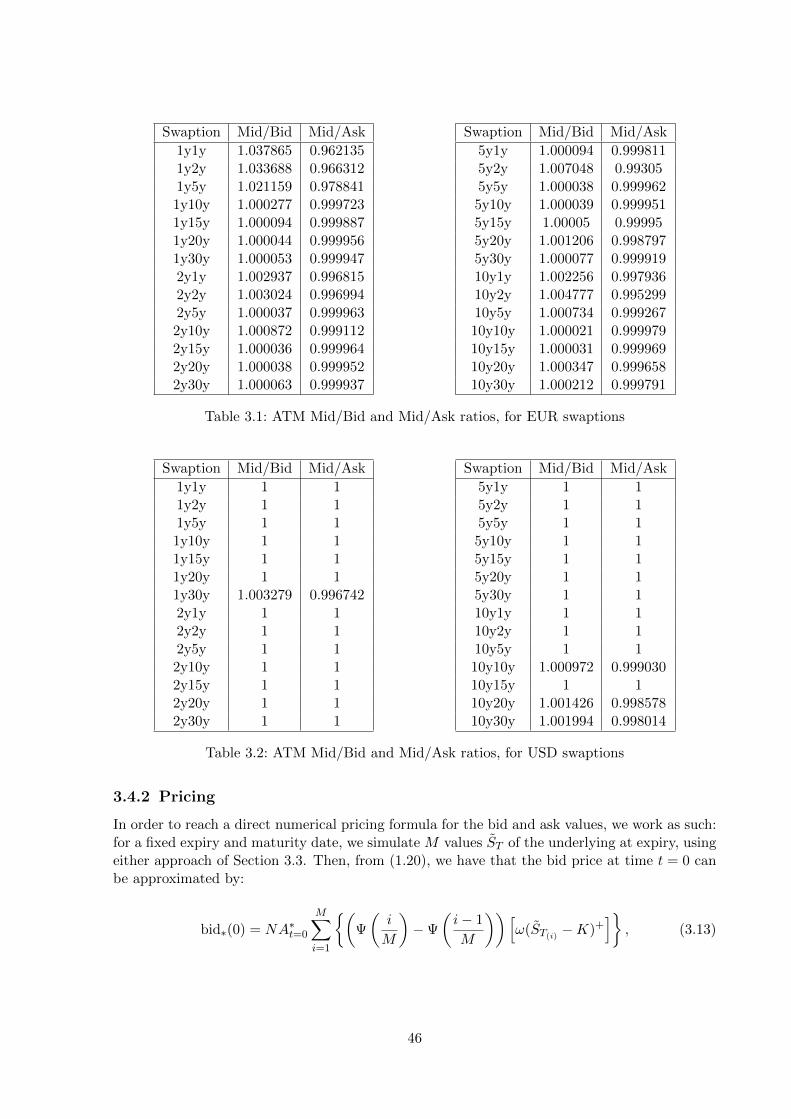
Swaption Mid/Bid Mid/Ask
1y1y 1.037865 0.9621351y2y 1.033688 0.9663121y5y 1.021159 0.9788411y10y 1.000277 0.9997231y15y 1.000094 0.9998871y20y 1.000044 0.9999561y30y 1.000053 0.9999472y1y 1.002937 0.9968152y2y 1.003024 0.9969942y5y 1.000037 0.9999632y10y 1.000872 0.9991122y15y 1.000036 0.9999642y20y 1.000038 0.9999522y30y 1.000063 0.999937
Swaption Mid/Bid Mid/Ask
5y1y 1.000094 0.9998115y2y 1.007048 0.993055y5y 1.000038 0.9999625y10y 1.000039 0.9999515y15y 1.00005 0.999955y20y 1.001206 0.9987975y30y 1.000077 0.99991910y1y 1.002256 0.99793610y2y 1.004777 0.99529910y5y 1.000734 0.99926710y10y 1.000021 0.99997910y15y 1.000031 0.99996910y20y 1.000347 0.99965810y30y 1.000212 0.999791
Table 3.1: ATM Mid/Bid and Mid/Ask ratios, for EUR swaptions
Swaption Mid/Bid Mid/Ask
1y1y 1 11y2y 1 11y5y 1 11y10y 1 11y15y 1 11y20y 1 11y30y 1.003279 0.9967422y1y 1 12y2y 1 12y5y 1 12y10y 1 12y15y 1 12y20y 1 12y30y 1 1
Swaption Mid/Bid Mid/Ask
5y1y 1 15y2y 1 15y5y 1 15y10y 1 15y15y 1 15y20y 1 15y30y 1 110y1y 1 110y2y 1 110y5y 1 110y10y 1.000972 0.99903010y15y 1 110y20y 1.001426 0.99857810y30y 1.001994 0.998014
Table 3.2: ATM Mid/Bid and Mid/Ask ratios, for USD swaptions
3.4.2 Pricing
In order to reach a direct numerical pricing formula for the bid and ask values, we work as such:for a fixed expiry and maturity date, we simulate M values ST of the underlying at expiry, usingeither approach of Section 3.3. Then, from (1.20), we have that the bid price at time t = 0 canbe approximated by:
bid∗(0) = NA∗t=0
M∑i=1
(Ψ
(i
M
)−Ψ
(i− 1
M
))[ω(ST(i) −K)+
], (3.13)
46
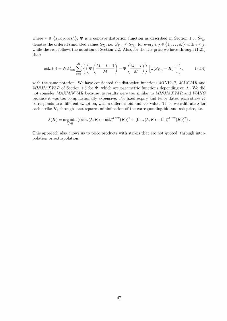
where ∗ ∈ swap, cash, Ψ is a concave distortion function as described in Section 1.5, ST(i)denotes the ordered simulated values STi , i.e. ST(i) ≤ ST(j) for every i, j ∈ 1, . . . ,M with i ≤ j,while the rest follows the notation of Section 2.2. Also, for the ask price we have through (1.21)that:
ask∗(0) = NA∗t=0
M∑i=1
(Ψ
(M − i+ 1
M
)−Ψ
(M − iM
))[ω(ST(i) −K)+
]. (3.14)
with the same notation. We have considered the distortion functions MINVAR, MAXVAR andMINMAXVAR of Section 1.6 for Ψ, which are parametric functions depending on λ. We didnot consider MAXMINVAR because its results were too similar to MINMAXVAR and WANGbecause it was too computationally expensive. For fixed expiry and tenor dates, each strike Kcorresponds to a different swaption, with a different bid and ask value. Thus, we calibrate λ foreach strike K, through least squares minimization of the corresponding bid and ask price, i.e.
λ(K) = arg minλ≥0
((ask∗(λ,K)− askMKT
∗ (K))2 + (bid∗(λ,K)− bidMKT∗ (K))2
).
This approach also allows us to price products with strikes that are not quoted, through inter-polation or extrapolation.
47
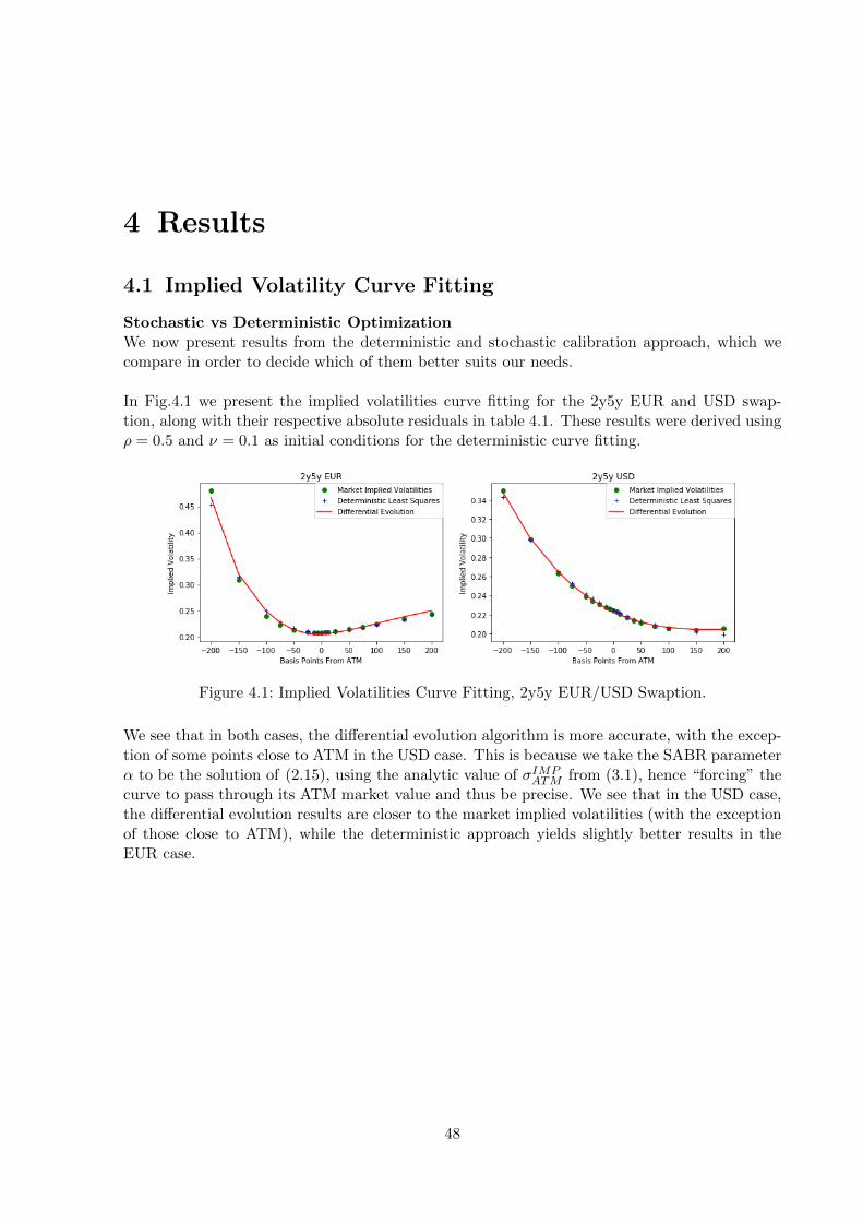
4 Results
4.1 Implied Volatility Curve Fitting
Stochastic vs Deterministic OptimizationWe now present results from the deterministic and stochastic calibration approach, which wecompare in order to decide which of them better suits our needs.
In Fig.4.1 we present the implied volatilities curve fitting for the 2y5y EUR and USD swap-tion, along with their respective absolute residuals in table 4.1. These results were derived usingρ = 0.5 and ν = 0.1 as initial conditions for the deterministic curve fitting.
Figure 4.1: Implied Volatilities Curve Fitting, 2y5y EUR/USD Swaption.
We see that in both cases, the differential evolution algorithm is more accurate, with the excep-tion of some points close to ATM in the USD case. This is because we take the SABR parameterα to be the solution of (2.15), using the analytic value of σIMP
ATM from (3.1), hence “forcing” thecurve to pass through its ATM market value and thus be precise. We see that in the USD case,the differential evolution results are closer to the market implied volatilities (with the exceptionof those close to ATM), while the deterministic approach yields slightly better results in theEUR case.
48
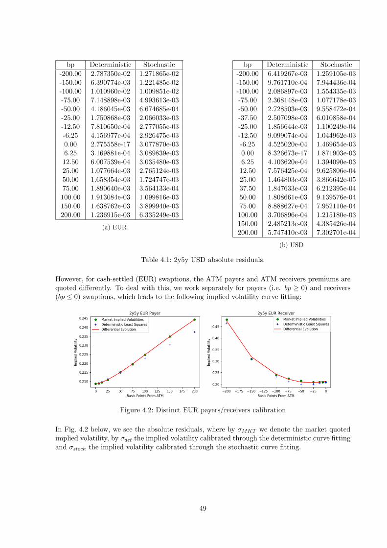
bp Deterministic Stochastic
-200.00 2.787350e-02 1.271865e-02-150.00 6.390774e-03 1.221485e-02-100.00 1.010960e-02 1.009851e-02-75.00 7.148898e-03 4.993613e-03-50.00 4.186045e-03 6.674685e-04-25.00 1.750868e-03 2.066033e-03-12.50 7.810650e-04 2.777055e-03-6.25 4.156977e-04 2.926475e-030.00 2.775558e-17 3.077870e-036.25 3.169881e-04 3.089839e-0312.50 6.007539e-04 3.035480e-0325.00 1.077664e-03 2.765124e-0350.00 1.658354e-03 1.724747e-0375.00 1.890640e-03 3.564133e-04100.00 1.913084e-03 1.099816e-03150.00 1.638762e-03 3.899940e-03200.00 1.236915e-03 6.335249e-03
(a) EUR
bp Deterministic Stochastic
-200.00 6.419267e-03 1.259105e-03-150.00 9.761710e-04 7.944436e-04-100.00 2.086897e-03 1.554335e-03-75.00 2.368148e-03 1.077178e-03-50.00 2.728503e-03 9.558472e-04-37.50 2.507098e-03 6.010858e-04-25.00 1.856644e-03 1.100249e-04-12.50 9.099074e-04 1.044962e-03-6.25 4.525020e-04 1.469654e-030.00 8.326673e-17 1.871903e-036.25 4.103620e-04 1.394090e-0312.50 7.576425e-04 9.625806e-0425.00 1.464803e-03 3.866642e-0537.50 1.847633e-03 6.212395e-0450.00 1.808661e-03 9.139576e-0475.00 8.888627e-04 7.952110e-04100.00 3.706896e-04 1.215180e-03150.00 2.485213e-03 4.385426e-04200.00 5.747410e-03 7.302701e-04
(b) USD
Table 4.1: 2y5y USD absolute residuals.
However, for cash-settled (EUR) swaptions, the ATM payers and ATM receivers premiums arequoted differently. To deal with this, we work separately for payers (i.e. bp ≥ 0) and receivers(bp ≤ 0) swaptions, which leads to the following implied volatility curve fitting:
Figure 4.2: Distinct EUR payers/receivers calibration
In Fig. 4.2 below, we see the absolute residuals, where by σMKT we denote the market quotedimplied volatility, by σdet the implied volatility calibrated through the deterministic curve fittingand σstoch the implied volatility calibrated through the stochastic curve fitting.
49
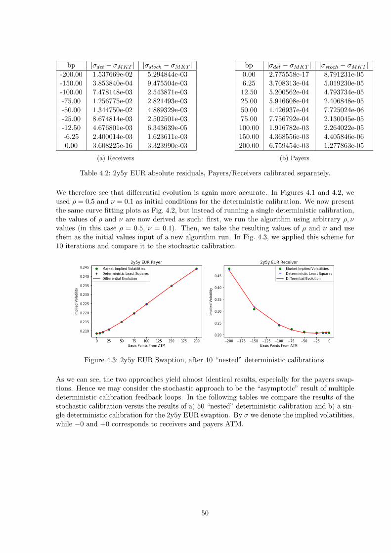
bp |σdet − σMKT | |σstoch − σMKT |-200.00 1.537669e-02 5.294844e-03-150.00 3.853840e-04 9.475504e-03-100.00 7.478148e-03 2.543871e-03-75.00 1.256775e-02 2.821493e-03-50.00 1.344750e-02 4.889329e-03-25.00 8.674814e-03 2.502501e-03-12.50 4.676801e-03 6.343639e-05-6.25 2.400014e-03 1.623611e-030.00 3.608225e-16 3.323990e-03
(a) Receivers
bp |σdet − σMKT | |σstoch − σMKT |0.00 2.775558e-17 8.791231e-056.25 3.708313e-04 5.019230e-0512.50 5.200562e-04 4.793734e-0525.00 5.916608e-04 2.406848e-0550.00 1.426937e-04 7.725024e-0675.00 7.756792e-04 2.130045e-05100.00 1.916782e-03 2.264022e-05150.00 4.368556e-03 4.405846e-06200.00 6.759454e-03 1.277863e-05
(b) Payers
Table 4.2: 2y5y EUR absolute residuals, Payers/Receivers calibrated separately.
We therefore see that differential evolution is again more accurate. In Figures 4.1 and 4.2, weused ρ = 0.5 and ν = 0.1 as initial conditions for the deterministic calibration. We now presentthe same curve fitting plots as Fig. 4.2, but instead of running a single deterministic calibration,the values of ρ and ν are now derived as such: first, we run the algorithm using arbitrary ρ, νvalues (in this case ρ = 0.5, ν = 0.1). Then, we take the resulting values of ρ and ν and usethem as the initial values input of a new algorithm run. In Fig. 4.3, we applied this scheme for10 iterations and compare it to the stochastic calibration.
Figure 4.3: 2y5y EUR Swaption, after 10 “nested” deterministic calibrations.
As we can see, the two approaches yield almost identical results, especially for the payers swap-tions. Hence we may consider the stochastic approach to be the “asymptotic” result of multipledeterministic calibration feedback loops. In the following tables we compare the results of thestochastic calibration versus the results of a) 50 “nested” deterministic calibration and b) a sin-gle deterministic calibration for the 2y5y EUR swaption. By σ we denote the implied volatilities,while −0 and +0 corresponds to receivers and payers ATM.
50
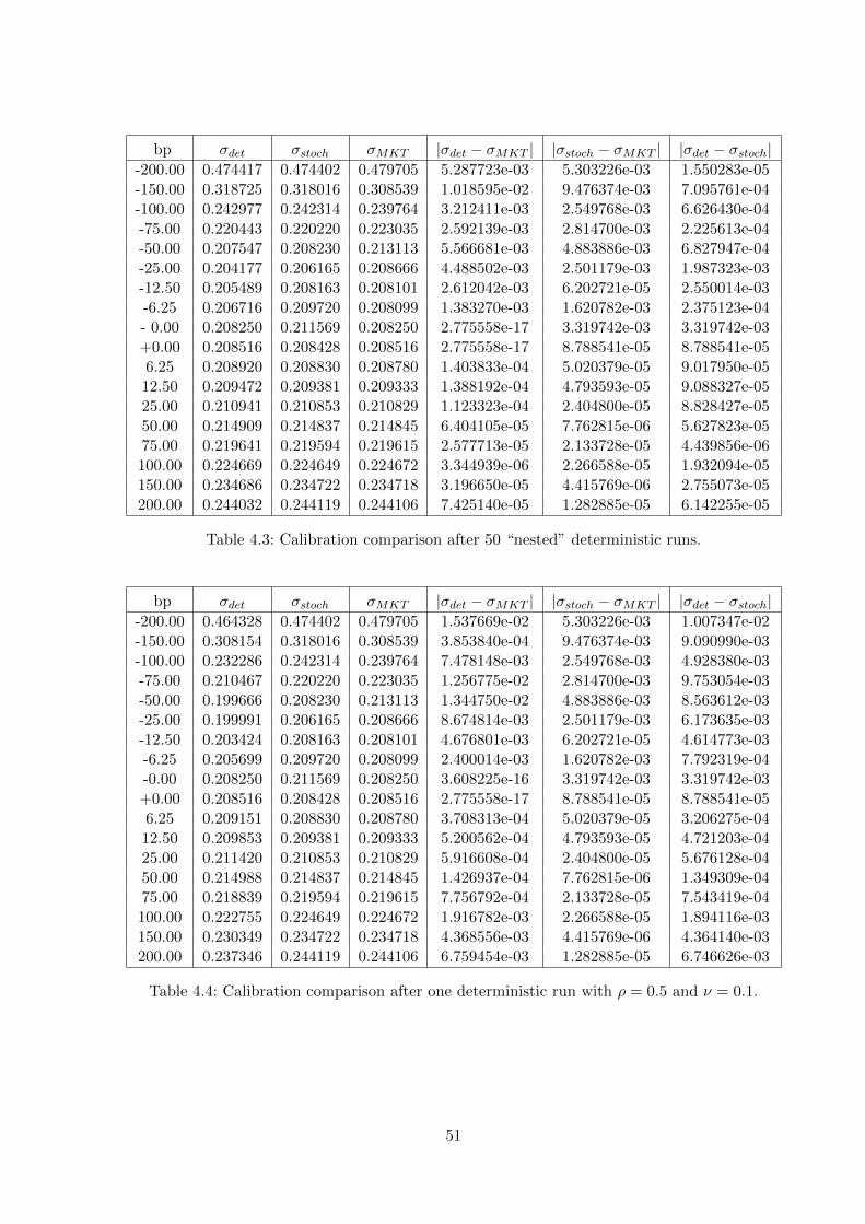
bp σdet σstoch σMKT |σdet − σMKT | |σstoch − σMKT | |σdet − σstoch|-200.00 0.474417 0.474402 0.479705 5.287723e-03 5.303226e-03 1.550283e-05-150.00 0.318725 0.318016 0.308539 1.018595e-02 9.476374e-03 7.095761e-04-100.00 0.242977 0.242314 0.239764 3.212411e-03 2.549768e-03 6.626430e-04-75.00 0.220443 0.220220 0.223035 2.592139e-03 2.814700e-03 2.225613e-04-50.00 0.207547 0.208230 0.213113 5.566681e-03 4.883886e-03 6.827947e-04-25.00 0.204177 0.206165 0.208666 4.488502e-03 2.501179e-03 1.987323e-03-12.50 0.205489 0.208163 0.208101 2.612042e-03 6.202721e-05 2.550014e-03-6.25 0.206716 0.209720 0.208099 1.383270e-03 1.620782e-03 2.375123e-04- 0.00 0.208250 0.211569 0.208250 2.775558e-17 3.319742e-03 3.319742e-03+0.00 0.208516 0.208428 0.208516 2.775558e-17 8.788541e-05 8.788541e-056.25 0.208920 0.208830 0.208780 1.403833e-04 5.020379e-05 9.017950e-0512.50 0.209472 0.209381 0.209333 1.388192e-04 4.793593e-05 9.088327e-0525.00 0.210941 0.210853 0.210829 1.123323e-04 2.404800e-05 8.828427e-0550.00 0.214909 0.214837 0.214845 6.404105e-05 7.762815e-06 5.627823e-0575.00 0.219641 0.219594 0.219615 2.577713e-05 2.133728e-05 4.439856e-06100.00 0.224669 0.224649 0.224672 3.344939e-06 2.266588e-05 1.932094e-05150.00 0.234686 0.234722 0.234718 3.196650e-05 4.415769e-06 2.755073e-05200.00 0.244032 0.244119 0.244106 7.425140e-05 1.282885e-05 6.142255e-05
Table 4.3: Calibration comparison after 50 “nested” deterministic runs.
bp σdet σstoch σMKT |σdet − σMKT | |σstoch − σMKT | |σdet − σstoch|-200.00 0.464328 0.474402 0.479705 1.537669e-02 5.303226e-03 1.007347e-02-150.00 0.308154 0.318016 0.308539 3.853840e-04 9.476374e-03 9.090990e-03-100.00 0.232286 0.242314 0.239764 7.478148e-03 2.549768e-03 4.928380e-03-75.00 0.210467 0.220220 0.223035 1.256775e-02 2.814700e-03 9.753054e-03-50.00 0.199666 0.208230 0.213113 1.344750e-02 4.883886e-03 8.563612e-03-25.00 0.199991 0.206165 0.208666 8.674814e-03 2.501179e-03 6.173635e-03-12.50 0.203424 0.208163 0.208101 4.676801e-03 6.202721e-05 4.614773e-03-6.25 0.205699 0.209720 0.208099 2.400014e-03 1.620782e-03 7.792319e-04-0.00 0.208250 0.211569 0.208250 3.608225e-16 3.319742e-03 3.319742e-03+0.00 0.208516 0.208428 0.208516 2.775558e-17 8.788541e-05 8.788541e-056.25 0.209151 0.208830 0.208780 3.708313e-04 5.020379e-05 3.206275e-0412.50 0.209853 0.209381 0.209333 5.200562e-04 4.793593e-05 4.721203e-0425.00 0.211420 0.210853 0.210829 5.916608e-04 2.404800e-05 5.676128e-0450.00 0.214988 0.214837 0.214845 1.426937e-04 7.762815e-06 1.349309e-0475.00 0.218839 0.219594 0.219615 7.756792e-04 2.133728e-05 7.543419e-04100.00 0.222755 0.224649 0.224672 1.916782e-03 2.266588e-05 1.894116e-03150.00 0.230349 0.234722 0.234718 4.368556e-03 4.415769e-06 4.364140e-03200.00 0.237346 0.244119 0.244106 6.759454e-03 1.282885e-05 6.746626e-03
Table 4.4: Calibration comparison after one deterministic run with ρ = 0.5 and ν = 0.1.
51
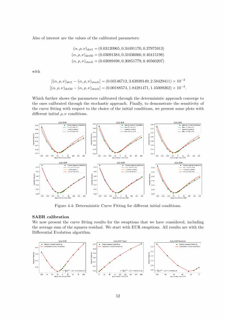
Also of interest are the values of the calibrated parameters:
(α, ρ, ν)det1 = (0.03120965, 0.34491170, 0.37975913)
(α, ρ, ν)det50 = (0.03091384, 0.31036060, 0.40415198)
(α, ρ, ν)stoch = (0.03089498, 0.30851779, 0.40560207)
with ∣∣(α, ρ, ν)det1 − (α, ρ, ν)stoch∣∣ = (0.03146712, 3.63939149, 2.58429411)× 10−2∣∣(α, ρ, ν)det50 − (α, ρ, ν)stoch∣∣ = (0.00188574, 1.84281471, 1.45009262)× 10−3.
Which further shows the parameters calibrated through the deterministic approach converge tothe ones calibrated through the stochastic approach. Finally, to demonstrate the sensitivity ofthe curve fitting with respect to the choice of the initial conditions, we present some plots withdifferent initial ρ, ν conditions.
Figure 4.4: Deterministic Curve Fitting for different initial conditions.
SABR calibrationWe now present the curve fitting results for the swaptions that we have considered, includingthe average sum of the squares residual. We start with EUR swaptions. All results are with theDifferential Evolution algorithm.
52
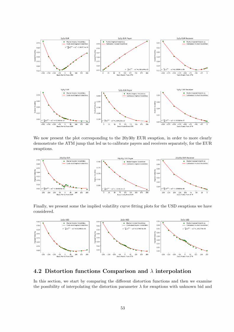
We now present the plot corresponding to the 20y30y EUR swaption, in order to more clearlydemonstrate the ATM jump that led us to calibrate payers and receivers separately, for the EURswaptions.
Finally, we present some the implied volatility curve fitting plots for the USD swaptions we haveconsidered.
4.2 Distortion functions Comparison and λ interpolation
In this section, we start by comparing the different distortion functions and then we examinethe possibility of interpolating the distortion parameter λ for swaptions with unknown bid and
53
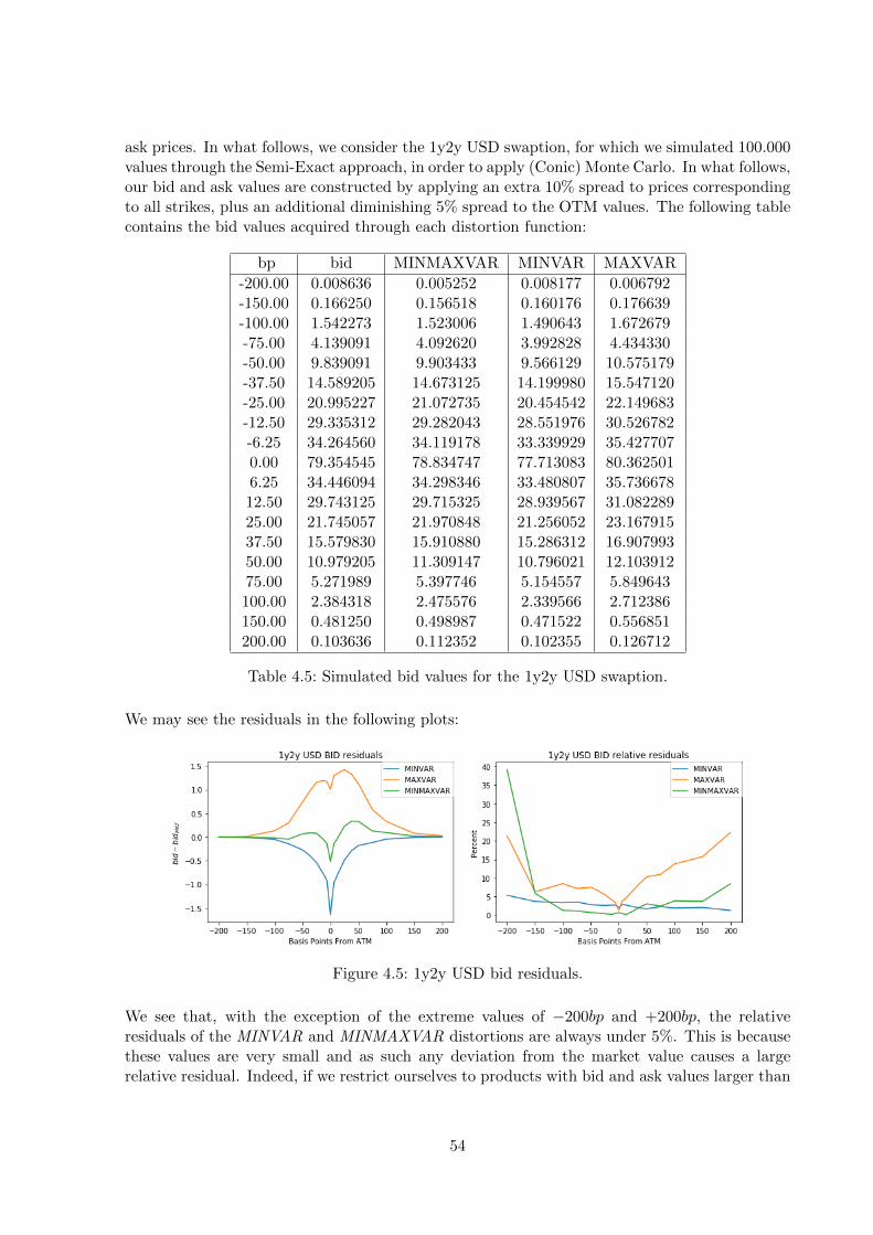
ask prices. In what follows, we consider the 1y2y USD swaption, for which we simulated 100.000values through the Semi-Exact approach, in order to apply (Conic) Monte Carlo. In what follows,our bid and ask values are constructed by applying an extra 10% spread to prices correspondingto all strikes, plus an additional diminishing 5% spread to the OTM values. The following tablecontains the bid values acquired through each distortion function:
bp bid MINMAXVAR MINVAR MAXVAR
-200.00 0.008636 0.005252 0.008177 0.006792-150.00 0.166250 0.156518 0.160176 0.176639-100.00 1.542273 1.523006 1.490643 1.672679-75.00 4.139091 4.092620 3.992828 4.434330-50.00 9.839091 9.903433 9.566129 10.575179-37.50 14.589205 14.673125 14.199980 15.547120-25.00 20.995227 21.072735 20.454542 22.149683-12.50 29.335312 29.282043 28.551976 30.526782-6.25 34.264560 34.119178 33.339929 35.4277070.00 79.354545 78.834747 77.713083 80.3625016.25 34.446094 34.298346 33.480807 35.73667812.50 29.743125 29.715325 28.939567 31.08228925.00 21.745057 21.970848 21.256052 23.16791537.50 15.579830 15.910880 15.286312 16.90799350.00 10.979205 11.309147 10.796021 12.10391275.00 5.271989 5.397746 5.154557 5.849643100.00 2.384318 2.475576 2.339566 2.712386150.00 0.481250 0.498987 0.471522 0.556851200.00 0.103636 0.112352 0.102355 0.126712
Table 4.5: Simulated bid values for the 1y2y USD swaption.
We may see the residuals in the following plots:
Figure 4.5: 1y2y USD bid residuals.
We see that, with the exception of the extreme values of −200bp and +200bp, the relativeresiduals of the MINVAR and MINMAXVAR distortions are always under 5%. This is becausethese values are very small and as such any deviation from the market value causes a largerelative residual. Indeed, if we restrict ourselves to products with bid and ask values larger than
54
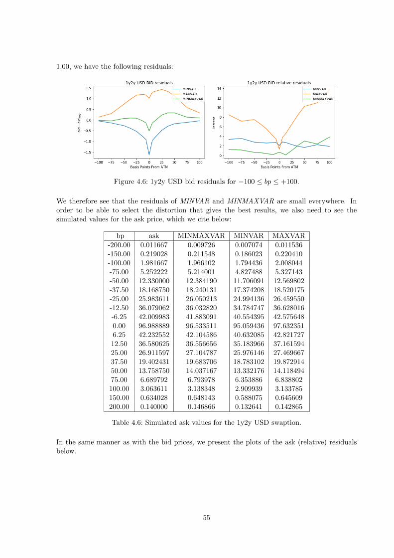
1.00, we have the following residuals:
Figure 4.6: 1y2y USD bid residuals for −100 ≤ bp ≤ +100.
We therefore see that the residuals of MINVAR and MINMAXVAR are small everywhere. Inorder to be able to select the distortion that gives the best results, we also need to see thesimulated values for the ask price, which we cite below:
bp ask MINMAXVAR MINVAR MAXVAR
-200.00 0.011667 0.009726 0.007074 0.011536-150.00 0.219028 0.211548 0.186023 0.220410-100.00 1.981667 1.966102 1.794436 2.008044-75.00 5.252222 5.214001 4.827488 5.327143-50.00 12.330000 12.384190 11.706091 12.569802-37.50 18.168750 18.240131 17.374208 18.520175-25.00 25.983611 26.050213 24.994136 26.459550-12.50 36.079062 36.032820 34.784747 36.628016-6.25 42.009983 41.883091 40.554395 42.5756480.00 96.988889 96.533511 95.059436 97.6323516.25 42.232552 42.104586 40.632085 42.82172712.50 36.580625 36.556656 35.183966 37.16159425.00 26.911597 27.104787 25.976146 27.46966737.50 19.402431 19.683706 18.783102 19.87291450.00 13.758750 14.037167 13.332176 14.11849475.00 6.689792 6.793978 6.353886 6.838802100.00 3.063611 3.138348 2.909939 3.133785150.00 0.634028 0.648143 0.588075 0.645609200.00 0.140000 0.146866 0.132641 0.142865
Table 4.6: Simulated ask values for the 1y2y USD swaption.
In the same manner as with the bid prices, we present the plots of the ask (relative) residualsbelow.
55
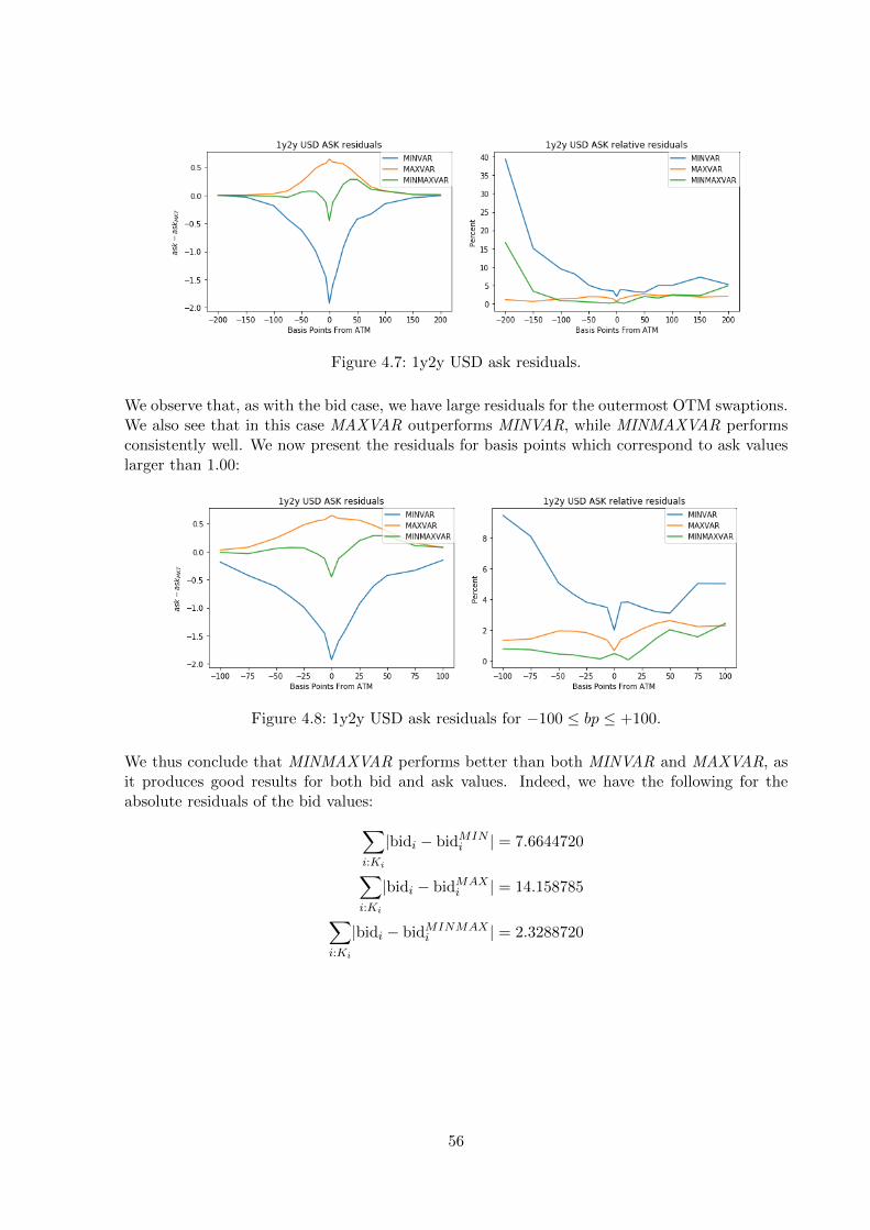
Figure 4.7: 1y2y USD ask residuals.
We observe that, as with the bid case, we have large residuals for the outermost OTM swaptions.We also see that in this case MAXVAR outperforms MINVAR, while MINMAXVAR performsconsistently well. We now present the residuals for basis points which correspond to ask valueslarger than 1.00:
Figure 4.8: 1y2y USD ask residuals for −100 ≤ bp ≤ +100.
We thus conclude that MINMAXVAR performs better than both MINVAR and MAXVAR, asit produces good results for both bid and ask values. Indeed, we have the following for theabsolute residuals of the bid values:∑
i:Ki
|bidi − bidMINi | = 7.6644720
∑i:Ki
|bidi − bidMAXi | = 14.158785
∑i:Ki
|bidi − bidMINMAXi | = 2.3288720
56
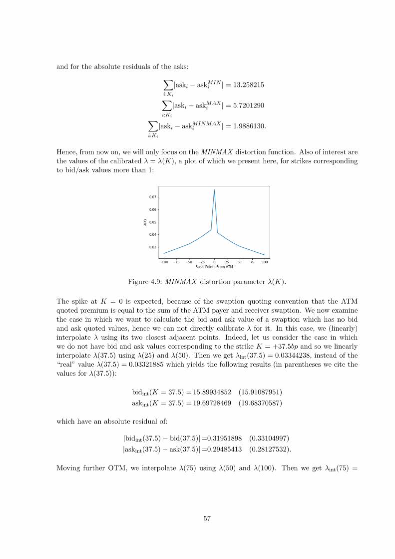
and for the absolute residuals of the asks:∑i:Ki
|aski − askMINi | = 13.258215
∑i:Ki
|aski − askMAXi | = 5.7201290
∑i:Ki
|aski − askMINMAXi | = 1.9886130.
Hence, from now on, we will only focus on the MINMAX distortion function. Also of interest arethe values of the calibrated λ = λ(K), a plot of which we present here, for strikes correspondingto bid/ask values more than 1:
Figure 4.9: MINMAX distortion parameter λ(K).
The spike at K = 0 is expected, because of the swaption quoting convention that the ATMquoted premium is equal to the sum of the ATM payer and receiver swaption. We now examinethe case in which we want to calculate the bid and ask value of a swaption which has no bidand ask quoted values, hence we can not directly calibrate λ for it. In this case, we (linearly)interpolate λ using its two closest adjacent points. Indeed, let us consider the case in whichwe do not have bid and ask values corresponding to the strike K = +37.5bp and so we linearlyinterpolate λ(37.5) using λ(25) and λ(50). Then we get λint(37.5) = 0.03344238, instead of the“real” value λ(37.5) = 0.03321885 which yields the following results (in parentheses we cite thevalues for λ(37.5)):
bidint(K = 37.5) = 15.89934852 (15.91087951)
askint(K = 37.5) = 19.69728469 (19.68370587)
which have an absolute residual of:
|bidint(37.5)− bid(37.5)|=0.31951898 (0.33104997)
|askint(37.5)− ask(37.5)|=0.29485413 (0.28127532).
Moving further OTM, we interpolate λ(75) using λ(50) and λ(100). Then we get λint(75) =
57
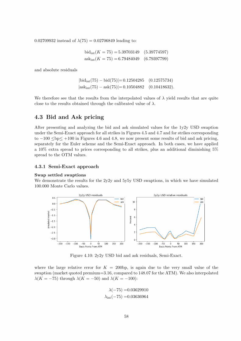
0.02709932 instead of λ(75) = 0.02706849 leading to:
bidint(K = 75) = 5.39703149 (5.39774597)
askint(K = 75) = 6.79484049 (6.79397799)
and absolute residuals
|bidint(75)− bid(75)|= 0.12504285 (0.12575734)
|askint(75)− ask(75)|= 0.10504882 (0.10418632).
We therefore see that the results from the interpolated values of λ yield results that are quiteclose to the results obtained through the calibrated value of λ.
4.3 Bid and Ask pricing
After presenting and analyzing the bid and ask simulated values for the 1y2y USD swaptionunder the Semi-Exact approach for all strikes in Figures 4.5 and 4.7 and for strikes correspondingto −100 ≤bp≤ +100 in Figures 4.6 and 4.8, we now present some results of bid and ask pricing,separately for the Euler scheme and the Semi-Exact approach. In both cases, we have applieda 10% extra spread to prices corresponding to all strikes, plus an additional diminishing 5%spread to the OTM values.
4.3.1 Semi-Exact approach
Swap settled swaptionsWe demonstrate the results for the 2y2y and 5y5y USD swaptions, in which we have simulated100.000 Monte Carlo values.
Figure 4.10: 2y2y USD bid and ask residuals, Semi-Exact.
where the large relative error for K = 200bp, is again due to the very small value of theswaption (market quoted premium=3.16, compared to 148.07 for the ATM). We also interpolatedλ(K = −75) through λ(K = −50) and λ(K = −100):
λ(−75) =0.03629910
λint(−75) =0.03636964
58
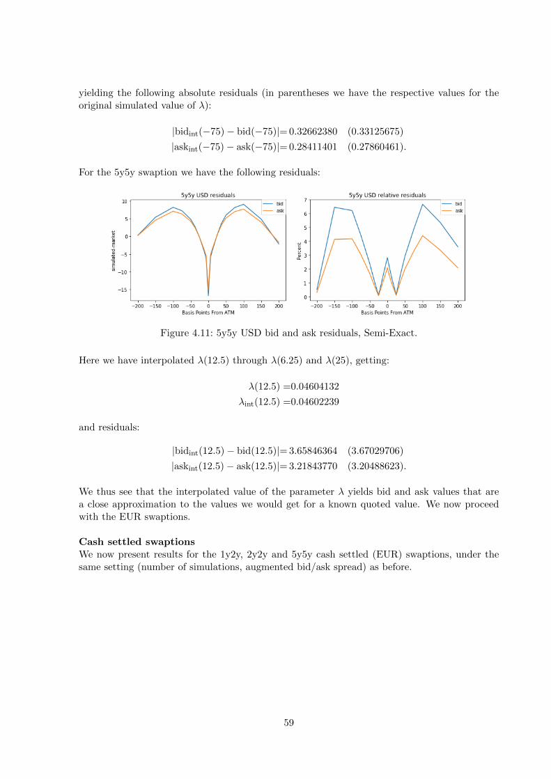
yielding the following absolute residuals (in parentheses we have the respective values for theoriginal simulated value of λ):
|bidint(−75)− bid(−75)|= 0.32662380 (0.33125675)
|askint(−75)− ask(−75)|= 0.28411401 (0.27860461).
For the 5y5y swaption we have the following residuals:
Figure 4.11: 5y5y USD bid and ask residuals, Semi-Exact.
Here we have interpolated λ(12.5) through λ(6.25) and λ(25), getting:
λ(12.5) =0.04604132
λint(12.5) =0.04602239
and residuals:
|bidint(12.5)− bid(12.5)|= 3.65846364 (3.67029706)
|askint(12.5)− ask(12.5)|= 3.21843770 (3.20488623).
We thus see that the interpolated value of the parameter λ yields bid and ask values that area close approximation to the values we would get for a known quoted value. We now proceedwith the EUR swaptions.
Cash settled swaptionsWe now present results for the 1y2y, 2y2y and 5y5y cash settled (EUR) swaptions, under thesame setting (number of simulations, augmented bid/ask spread) as before.
59
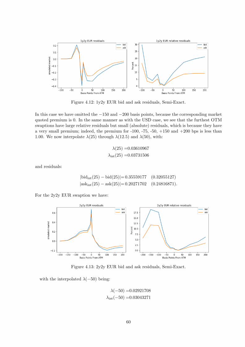
Figure 4.12: 1y2y EUR bid and ask residuals, Semi-Exact.
In this case we have omitted the −150 and −200 basis points, because the corresponding marketquoted premium is 0. In the same manner as with the USD case, we see that the furthest OTMswaptions have large relative residuals but small (absolute) residuals, which is because they havea very small premium; indeed, the premium for -100, -75, -50, +150 and +200 bps is less than1.00. We now interpolate λ(25) through λ(12.5) and λ(50), with:
λ(25) =0.03610967
λint(25) =0.03731506
and residuals:
|bidint(25)− bid(25)|= 0.35559177 (0.32055127)
|askint(25)− ask(25)|= 0.20271702 (0.24816871).
For the 2y2y EUR swaption we have:
Figure 4.13: 2y2y EUR bid and ask residuals, Semi-Exact.
with the interpolated λ(−50) being:
λ(−50) =0.02921708
λint(−50) =0.03043271
60
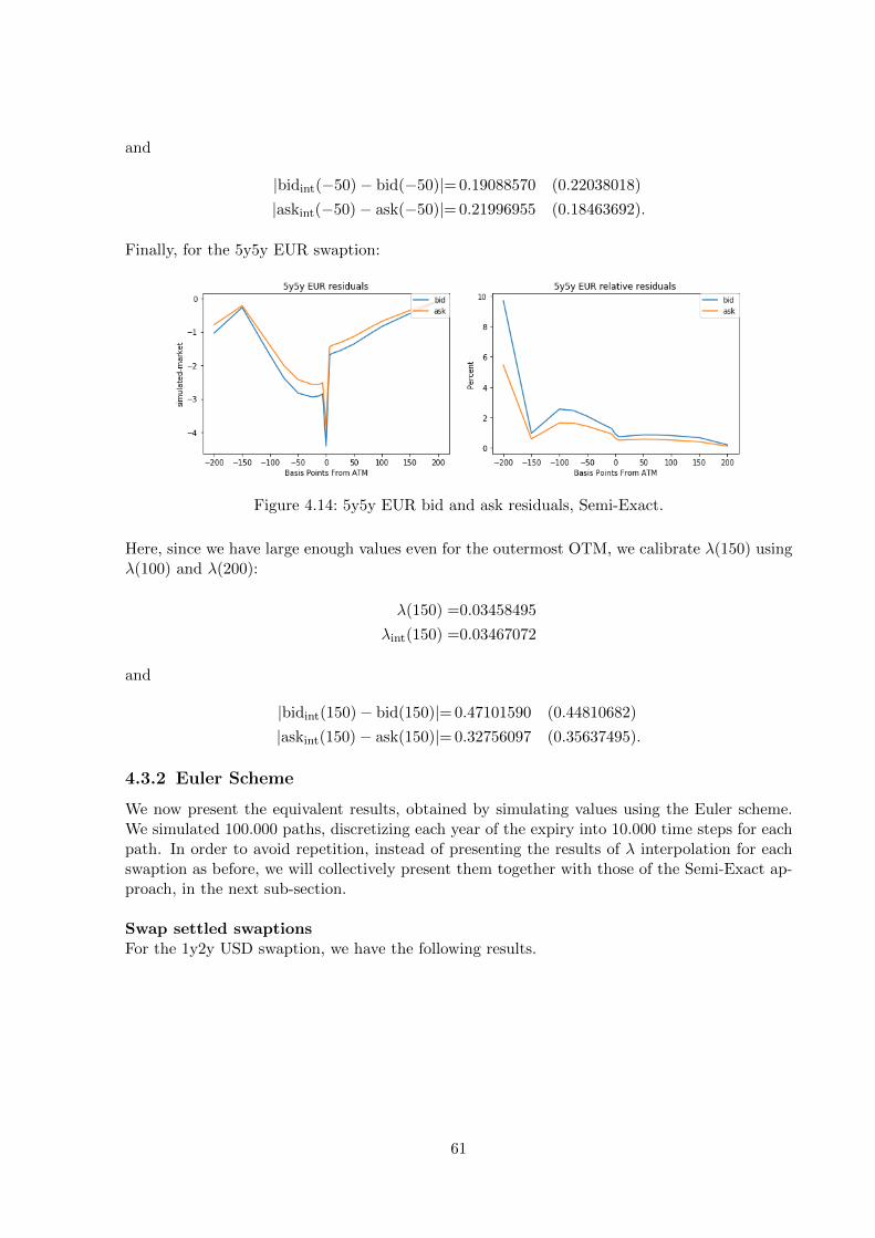
and
|bidint(−50)− bid(−50)|= 0.19088570 (0.22038018)
|askint(−50)− ask(−50)|= 0.21996955 (0.18463692).
Finally, for the 5y5y EUR swaption:
Figure 4.14: 5y5y EUR bid and ask residuals, Semi-Exact.
Here, since we have large enough values even for the outermost OTM, we calibrate λ(150) usingλ(100) and λ(200):
λ(150) =0.03458495
λint(150) =0.03467072
and
|bidint(150)− bid(150)|= 0.47101590 (0.44810682)
|askint(150)− ask(150)|= 0.32756097 (0.35637495).
4.3.2 Euler Scheme
We now present the equivalent results, obtained by simulating values using the Euler scheme.We simulated 100.000 paths, discretizing each year of the expiry into 10.000 time steps for eachpath. In order to avoid repetition, instead of presenting the results of λ interpolation for eachswaption as before, we will collectively present them together with those of the Semi-Exact ap-proach, in the next sub-section.
Swap settled swaptionsFor the 1y2y USD swaption, we have the following results.
61
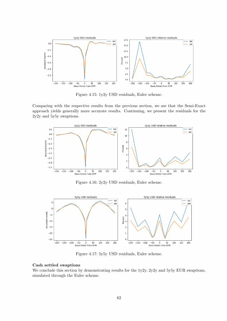
Figure 4.15: 1y2y USD residuals, Euler scheme.
Comparing with the respective results from the previous section, we see that the Semi-Exactapproach yields generally more accurate results. Continuing, we present the residuals for the2y2y and 5y5y swaptions.
Figure 4.16: 2y2y USD residuals, Euler scheme.
Figure 4.17: 5y5y USD residuals, Euler scheme.
Cash settled swaptionsWe conclude this section by demonstrating results for the 1y2y, 2y2y and 5y5y EUR swaptions,simulated through the Euler scheme.
62
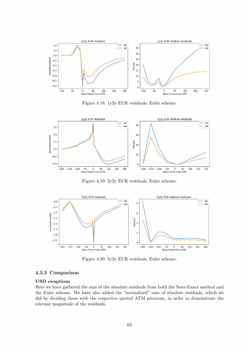
Figure 4.18: 1y2y EUR residuals, Euler scheme.
Figure 4.19: 2y2y EUR residuals, Euler scheme.
Figure 4.20: 5y5y EUR residuals, Euler scheme.
4.3.3 Comparison
USD swaptionsHere we have gathered the sum of the absolute residuals from both the Semi-Exact method andthe Euler scheme. We have also added the “normalized” sum of absolute residuals, which wedid by dividing them with the respective quoted ATM premium, in order to demonstrate therelevant magnitude of the residuals.
63
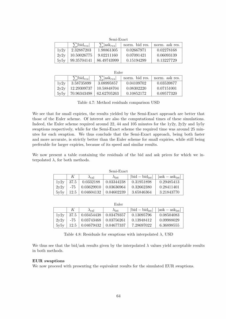
Semi-Exact∑|bidres|
∑|askres| norm. bid res. norm. ask res.
1y2y 2.32887203 1.98861305 0.02667971 0.022781682y2y 10.50026775 9.02211160 0.07091421 0.060931395y5y 99.35704141 86.49743999 0.15194299 0.13227729
Euler∑|bidres|
∑|askres| norm. bid res. norm. ask res.
1y2y 3.58735899 3.08995857 0.04109702 0.035398772y2y 12.29309737 10.58848704 0.08302220 0.071510015y5y 70.96343498 62.62705263 0.10852172 0.09577320
Table 4.7: Method residuals comparison USD
We see that for small expiries, the results yielded by the Semi-Exact approach are better thatthose of the Euler scheme. Of interest are also the computational times of these simulations.Indeed, the Euler scheme required around 22, 44 and 105 minutes for the 1y2y, 2y2y and 5y5yswaptions respectively, while for the Semi-Exact scheme the required time was around 25 min-utes for each swaption. We thus conclude that the Semi-Exact approach, being both fasterand more accurate, is strictly better than the Euler scheme for small expiries, while still beingpreferable for larger expiries, because of its speed and similar results.
We now present a table containing the residuals of the bid and ask prices for which we in-terpolated λ, for both methods.
Semi-Exact
K λcal λint |bid− bidint| |ask− askint|1y2y 37.5 0.0332188 0.03344238 0.31951898 0.294854132y2y -75 0.03629910 0.03636964 0.32662380 0.284114015y5y 12.5 0.04604132 0.04602239 3.65846364 3.21843770
Euler
K λcal λint |bid− bidint| |ask− askint|1y2y 37.5 0.03454438 0.03479357 0.13095796 0.085040832y2y -75 0.03743468 0.03756261 0.13948412 0.099880295y5y 12.5 0.04679432 0.04677337 7.28697022 6.36898555
Table 4.8: Residuals for swaptions with interpolated λ, USD
We thus see that the bid/ask results given by the interpolated λ values yield acceptable resultsin both methods.
EUR swaptionsWe now proceed with presenting the equivalent results for the simulated EUR swaptions.
64
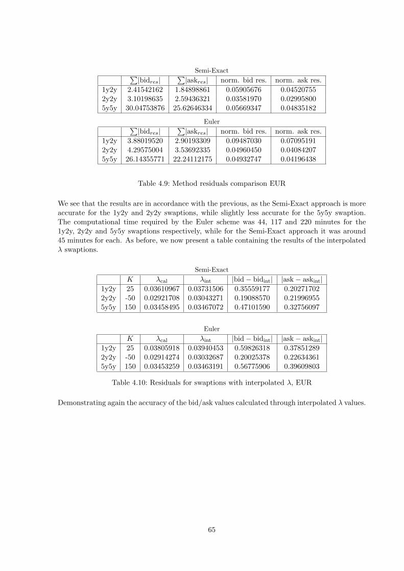
Semi-Exact∑|bidres|
∑|askres| norm. bid res. norm. ask res.
1y2y 2.41542162 1.84898861 0.05905676 0.045207552y2y 3.10198635 2.59436321 0.03581970 0.029958005y5y 30.04753876 25.62646334 0.05669347 0.04835182
Euler∑|bidres|
∑|askres| norm. bid res. norm. ask res.
1y2y 3.88019520 2.90193309 0.09487030 0.070951912y2y 4.29575004 3.53692335 0.04960450 0.040842075y5y 26.14355771 22.24112175 0.04932747 0.04196438
Table 4.9: Method residuals comparison EUR
We see that the results are in accordance with the previous, as the Semi-Exact approach is moreaccurate for the 1y2y and 2y2y swaptions, while slightly less accurate for the 5y5y swaption.The computational time required by the Euler scheme was 44, 117 and 220 minutes for the1y2y, 2y2y and 5y5y swaptions respectively, while for the Semi-Exact approach it was around45 minutes for each. As before, we now present a table containing the results of the interpolatedλ swaptions.
Semi-Exact
K λcal λint |bid− bidint| |ask− askint|1y2y 25 0.03610967 0.03731506 0.35559177 0.202717022y2y -50 0.02921708 0.03043271 0.19088570 0.219969555y5y 150 0.03458495 0.03467072 0.47101590 0.32756097
Euler
K λcal λint |bid− bidint| |ask− askint|1y2y 25 0.03805918 0.03940453 0.59826318 0.378512892y2y -50 0.02914274 0.03032687 0.20025378 0.226343615y5y 150 0.03453259 0.03463191 0.56775906 0.39609803
Table 4.10: Residuals for swaptions with interpolated λ, EUR
Demonstrating again the accuracy of the bid/ask values calculated through interpolated λ values.
65
Discussion
The purpose of this thesis was to provide a pricing procedure for the bid and ask values of EURand USD swaptions, through the Conic Finance theory. To the best of our knowledge, this wasthe first such attempt. To do so, we had to calibrate the SABR parameters by curve fitting themarket implied volatilities and then, using them we simulated multiple values of the underlyingwhich were used for Conic Monte Carlo. To this end, we first applied two standard techniquesused in finance, i.e. using deterministic square minimization for the implied volatility curve fit-ting and simulating the underlying through the Euler discretization scheme. Then, we appliedtwo less frequently used techniques: the Differential Evolution algorithm for the parameter cal-ibration and the Semi-Exact approach for the underlying simulation. We concluded that bothDifferential Evolution and the Semi-Exact approach were better suited for our situation, thefirst being independent of potentially ill-chosen initial values and the second being less biasedand of far better computational speed.
Given our bid and ask results, we are led to the conclusion that the Conic Finance theoryoffers a solid pricing framework, which is valid in both liquid and illiquid markets.
Concerning future research, we have the following suggestions. Firstly, the products that weconsidered were liquid enough to have an almost zero bid-ask spread. We circumvented this byadding an artificial extra spread, but it would have been more natural to apply our study toless liquid products, something that we suggest for further studies. Continuing, even though wedemonstrated that the MINMAXVAR distortion function yielded the best results in our case,there is still room for improvement, namely considering the MINMAXVAR2 distortion function,as seen in [32], which is dependent on two parameters λ, γ instead of just one. This functionwould clearly require more computational time for calibration purposes, but offers greater versa-tility and as such should yield better results. Continuing, an open, to the best of our knowledge,problem in finance is the issue of the cash-settled (EUR) annuity. As discussed in Section 2.2,the current standard market formula is mathematically wrong, because of the use of the MultiCurve Framework. One suggestion would be to consider the cash-settled annuity as a stochasticprocess of its own and try to model it separately. Further, the poorer results of the Semi-Exactapproach for larger expiries are expected and discussed in Cai et al. [7], who offer the solution ofsplitting the expiry into smaller time intervals and applying the Semi-Exact piece-wise. Finally,instead of the classical Euler discretization scheme, we would suggest the use of a modified Eulerscheme that guarantees convergence for models with non-Lipschitz parameters, as seen e.g. in [4]and [6].
66
Popular summary
If the market is liquid and complete, then the classical financial framework offers an unambiguouspricing method for all financial products, through the use of the risk-neutral measure. We thushave the rule of the “one price”. However, in illiquid markets, the price of a product dependson the market direction, i.e. whether it is being bought or sold. This leads to the differencebetween the buying and the selling price, called the“bid-ask spread”, to become non-negligible.Conic Finance offers a framework in which easy to compute formulas are derived for the directcalculation of both the bid and the ask prices.
The SABR (“Stochastic Alpha Beta Rho”) model is a stochastic volatility model used to calcu-late forward values of a derivative’s underlying, for example the price of a stock or an interestrate. In the current post-crisis environment, interest rates are very low and sometimes evennegative. To deal with this situation, the Displaced SABR extension of SABR was developed.
In this thesis, we follow the Conic Finance approach and use the Displaced SABR model in orderto directly price the bid and ask prices of swaptions, i.e. derivatives in which the underlying isa swap. To do so, we first needed to calibrate the SABR parameters and then simulate multiplevalues of the underlying. In both cases, we used a well-known (deterministic least squares andEuler discretization) and a less known method (Differential Evolution Algorithm, “Semi-Exact”approach). We concluded that for the parameter calibration the Differential Evolution algo-rithm yielded better results and for the underlying simulation the Semi-Exact approach wasmore accurate in most cases and computationally less expensive in general.
67
Bibliography
[1] Joseph Abate and Ward Whitt. The fourier-series method for inverting transforms ofprobability distributions. Queueing systems, 10(1-2):5–87, 1992.
[2] Alexandre Antonov, Michael Konikov, and Michael Spector. The free boundary sabr: nat-ural extension to negative rates. Risk Magazine, pages 58–63, August 2015.
[3] Philippe Artzner, Freddy Delbaen, Jean-Marc Eber, and David Heath. Coherent measuresof risk. Mathematical finance, 9(3):203–228, 1999.
[4] Abdel Berkaoui, Mireille Bossy, and Awa Diop. Euler scheme for SDEs with non-lipschitzdiffusion coefficient: strong convergence. ESAIM: Probability and Statistics, 12:1–11, 2008.
[5] Fischer Black. The pricing of commodity contracts. Journal of financial economics, 3(1-2):167–179, 1976.
[6] Mireille Bossy and Awa Diop. An efficient discretisation scheme for one dimensional SDEswith a diffusion coefficient function of the form |x|α, α ∈[1/2, 1). PhD thesis, INRIA, 2007.
[7] Ning Cai, Yingda Song, and Nan Chen. Exact simulation of the sabr model. OperationsResearch, 65(4):931–951, 2017.
[8] Peter Carr, Helyette Geman, and Dilip B Madan. Pricing and hedging in incompletemarkets. Journal of financial economics, 62(1):131–167, 2001.
[9] Alexander Cherny and Dilip Madan. New measures for performance evaluation. The Reviewof Financial Studies, 22(7):2571–2606, 2008.
[10] Gustave Choquet. Theory of capacities. In Annales de l’institut Fourier, volume 5, pages131–295, 1954.
[11] Thomas E Copeland and Dan Galai. Information effects on the bid-ask spread. The Journalof Finance, 38(5):1457–1469, 1983.
[12] Freddy Delbaen. Coherent risk measures on general probability spaces. In Advances infinance and stochastics, pages 1–37. Springer, 2002.
[13] Dieter Denneberg. Non-additive measure and integral, volume 27. Springer Science &Business Media, 2013.
[14] Bruno Dupire. Pricing with a smile. Risk Magazine, 7(1):18–20, 1994.
[15] Ernst Eberlein, Dilip Madan, Martijn Pistorius, Wim Schoutens, and Marc Yor. Two priceeconomies in continuous time. Annals of Finance, 10(1):71–100, 2014.
[16] Damir Filipovic. Term-Structure Models. A Graduate Course. Springer, 2009.
68
[17] Hans Follmer and Alexander Schied. Stochastic finance: an introduction in discrete time.Walter de Gruyter, 2011.
[18] John Fulcher. Computational intelligence: an introduction. In Computational intelligence:a compendium, pages 3–78. Springer, 2008.
[19] Patrick S Hagan, Deep Kumar, Andrew S Lesniewski, and Diana E Woodward. Managingsmile risk. The Best of Wilmott, 1:249–296, 2002.
[20] Patrick S Hagan, Deep Kumar, Andrew S Lesniewski, and Diana E Woodward. Arbitrage-free SABR. Wilmott, 2014(69):60–75, 2014.
[21] Marc Henrard. Interest rate modelling in the multi-curve framework: Foundations, evolutionand implementation. Springer, 2014.
[22] Peter J Huber. Robust statistics. Wiley, New York, 1981.
[23] John Hull and Alan White. LIBOR vs. OIS: The derivatives discounting dilemma. JournalOf Investment Management, 11(3):14–27, 2013.
[24] John C Hull. Option, Futures and Other Derivatives. London: Pearson Education Ltd.,2012.
[25] Stefano M Iacus. Simulation and inference for stochastic differential equations: with Rexamples. Springer Science & Business Media, 2009.
[26] Othmane Islah. Solving SABR in exact form and unifying it with LIBOR market model.Working paper, 2009.
[27] Shigeo Kusuoka. On law invariant coherent risk measures: Mathematical finance. Advancesin Mathematical Economics, 3:8–95, 2001.
[28] Roger Lord, Remmert Koekkoek, and Dick Van Dijk. A comparison of biased simulationschemes for stochastic volatility models. Quantitative Finance, 10(2):177–194, 2010.
[29] Dilip Madan and Wim Schoutens. Applied Conic Finance. Cambridge University Press,2016.
[30] Dilip B Madan and Alexander Cherny. Markets as a counterparty: an introduction to conicfinance. International Journal of Theoretical and Applied Finance, 13(08):1149–1177, 2010.
[31] Dilip B Madan and Wim Schoutens. Conic financial markets and corporate finance. Eu-random Report, 2010.
[32] Dilip B Madan and Wim Schoutens. Conic coconuts: the pricing of contingent capital notesusing conic finance. Mathematics and Financial Economics, 4(2):87–106, 2011.
[33] Fabio Mercurio. No-arbitrage conditions for cash-settled swaptions. Technical report, BancaIMI. 2, 2007.
[34] Magnus Erik Hvass Pedersen. Tuning & simplifying heuristical optimization. PhD thesis,University of Southampton, 2010.
69

[35] Raoul Pietersz and Frank Sengers. A new pricing model for cash-settled swaptions. Workingpaper, 2017.
[36] Fabrice Douglas Rouah. The SABR model. Lecture notes, 2007.
[37] Rainer Storn and Kenneth Price. Differential evolution–a simple and efficient heuristic forglobal optimization over continuous spaces. Journal of global optimization, 11(4):341–359,1997.
[38] Marc Yor. Loi de l’indice du lacet brownien, et distribution de hartman-watson. Zeitschriftfur Wahrscheinlichkeitstheorie und verwandte Gebiete, 53(1):71–95, 1980.
70