Conic Linear Programming - web.stanford.edu · Computer Science Department of the University of Minnesota and met a young ... 1.6 Notes ... 2.1.1 Dual of conic linear programming

Conic Linear Programming

Yinyu Ye

December 2004, revised October 2017

i

ii

Preface

This monograph is developed for MS&E 314, “Conic Linear Programming”,which I am teaching at Stanford. Information, lecture slides, supporting mate-rials, and computer programs related to this book may be found at the followingaddress on the World-Wide Web:

http://www.stanford.edu/class/msande314Please report any question, comment and error to the address:

[email protected] little story in the development of semidefinite programming (SDP), a

major subclass of conic linear programming. One day in 1990, I visited theComputer Science Department of the University of Minnesota and met a younggraduate student, Farid Alizadeh. He, working then on combinatorial optimiza-tion, introduced me “semidefinite optimization” or linear programming over thepositive definite matrix cone. We had a very extensive discussion that afternoonand concluded that interior-point linear programming algorithms could be ap-plicable to solving SDPs. I suggested Farid to look at the linear programming(LP) interior-point algorithms and to develop an SDP (primal) potential reduc-tion algorithm. He worked hard for several months, and one afternoon showedup in my office in Iowa City, about 300 miles from Minneapolis. He had every-thing worked out, including potential function, algorithm, complexity bound,and even a “dictionary” list between LP and SDP. But he was stuck on oneproblem that was on how to keep the symmetry of the scaled directional ma-trix. We went to a bar nearby on Clinton Street in Iowa City (I paid for himsince I was a third-year professor then and eager to demonstrate that I couldtake care of my students). After chatting for a while, I suggested that he shoulduse scaling X−1/2∆X−1/2 to compute symmetric directional matrix ∆, insteadof X−1∆ which he was using earlier, where X is the current symmetric positivedefinite matrix. This way, X + α∆ would remain symmetric with a step-sizescalar. He returned to Minneapolis and moved to Berkeley shortly after, and fewweeks later sent me an e-mail message telling me that everything had workedout beautifully.

At the same time, Nesterov and Nemirovskii developed a more general andpowerful theory in extending interior-point algorithms for solving convex pro-grams, where SDP was a special case. Boyd and his group presented a widerange of SDP applications and formulations, many of which were incrediblynovel and elegant. Then came the primal-dual algorithms of many authors, the

iii

iv PREFACE

SDP approximation algorithm for Max-Cut, ... – SDP eventually establishedits full popularity.

PREFACE v

To Daisun, Fei, Tim, Kaylee and Rylee

vi PREFACE

Contents

Preface iii

List of Figures xi

1 Introduction and Preliminaries 11.1 Introduction . . . . . . . . . . . . . . . . . . . . . . . . . . . . . . 11.2 Mathematical Preliminaries . . . . . . . . . . . . . . . . . . . . . 3

1.2.1 Basic notations . . . . . . . . . . . . . . . . . . . . . . . . 31.2.2 Convex sets and cones . . . . . . . . . . . . . . . . . . . . 51.2.3 Real functions . . . . . . . . . . . . . . . . . . . . . . . . 101.2.4 Inequalities . . . . . . . . . . . . . . . . . . . . . . . . . . 12

1.3 Some Basic Decision and Optimization Problems . . . . . . . . . 131.3.1 System of linear equations . . . . . . . . . . . . . . . . . . 131.3.2 Linear least-squares problem . . . . . . . . . . . . . . . . 141.3.3 System of linear inequalities . . . . . . . . . . . . . . . . . 151.3.4 Linear programming (LP) . . . . . . . . . . . . . . . . . . 161.3.5 Quadratic programming (QP) . . . . . . . . . . . . . . . . 19

1.4 Algorithms and Computations . . . . . . . . . . . . . . . . . . . 201.4.1 Complexity of problems . . . . . . . . . . . . . . . . . . . 201.4.2 Convergence rate . . . . . . . . . . . . . . . . . . . . . . . 21

1.5 Basic Computational Procedures . . . . . . . . . . . . . . . . . . 231.5.1 Gaussian elimination method . . . . . . . . . . . . . . . . 231.5.2 Choleski decomposition method . . . . . . . . . . . . . . . 241.5.3 The Newton method . . . . . . . . . . . . . . . . . . . . . 241.5.4 Solving ball-constrained linear problem . . . . . . . . . . 251.5.5 Solving ball-constrained quadratic problem . . . . . . . . 26

1.6 Notes . . . . . . . . . . . . . . . . . . . . . . . . . . . . . . . . . 261.7 Exercises . . . . . . . . . . . . . . . . . . . . . . . . . . . . . . . 27

2 Conic Linear Programming 312.1 Conic Linear Programming and its Dual . . . . . . . . . . . . . . 31

2.1.1 Dual of conic linear programming . . . . . . . . . . . . . . 332.2 Farkas’ Lemma and Duality Theorem of Conic Linear Programming 35

2.2.1 Alternative theorem for conic systems . . . . . . . . . . . 36

vii

viii CONTENTS

2.2.2 Duality theorem for conic linear programming . . . . . . . 382.2.3 Optimality conditions of conic linear programming . . . . 40

2.3 Exact Low-Rank SDP Solutions . . . . . . . . . . . . . . . . . . . 422.3.1 Exact low-rank theorem . . . . . . . . . . . . . . . . . . . 42

2.4 Approximate Low-Rank SDP Solutions . . . . . . . . . . . . . . . 452.4.1 Approximate low-rank theorem . . . . . . . . . . . . . . . 452.4.2 A constructive proof . . . . . . . . . . . . . . . . . . . . . 47

2.5 Uniqueness of CLP Optimal Solution . . . . . . . . . . . . . . . . 512.6 Notes . . . . . . . . . . . . . . . . . . . . . . . . . . . . . . . . . 532.7 Exercises . . . . . . . . . . . . . . . . . . . . . . . . . . . . . . . 54

3 Interior-Point Algorithms 573.1 Central Path and Path-Following . . . . . . . . . . . . . . . . . . 57

3.1.1 Logarithmic barrier function for convex cones . . . . . . . 583.1.2 The central path . . . . . . . . . . . . . . . . . . . . . . . 633.1.3 Path following algorithms . . . . . . . . . . . . . . . . . . 67

3.2 Potential Reduction Algorithms . . . . . . . . . . . . . . . . . . . 693.2.1 Potential functions . . . . . . . . . . . . . . . . . . . . . . 703.2.2 Potential reduction algorithms . . . . . . . . . . . . . . . 723.2.3 Analysis of the primal potential-reduction . . . . . . . . . 74

3.3 Primal-Dual (Symmetric) Algorithm for LP and SDP . . . . . . 843.4 Dual Algorithm for SDP . . . . . . . . . . . . . . . . . . . . . . . 873.5 Initialization . . . . . . . . . . . . . . . . . . . . . . . . . . . . . 953.6 Notes . . . . . . . . . . . . . . . . . . . . . . . . . . . . . . . . . 983.7 Exercises . . . . . . . . . . . . . . . . . . . . . . . . . . . . . . . 98

4 SDP for Global Quadratic and Combinatorial Optimization 1014.1 Approximation . . . . . . . . . . . . . . . . . . . . . . . . . . . . 1014.2 Ball-Constrained Quadratic Minimization . . . . . . . . . . . . . 102

4.2.1 Homogeneous Case: q = 0 . . . . . . . . . . . . . . . . . . 1024.2.2 Non-Homogeneous Case . . . . . . . . . . . . . . . . . . . 103

4.3 Quadratically Constrained Quadratic Problems (QCQP) . . . . . 1044.3.1 Multiple Ellipsoid-Constrained Quadratic Maximization . 1054.3.2 Binary Quadratic Maximization . . . . . . . . . . . . . . 1064.3.3 Box Constrained Optimization . . . . . . . . . . . . . . . 107

4.4 Max-Cut Problem . . . . . . . . . . . . . . . . . . . . . . . . . . 1124.4.1 SDP relaxation . . . . . . . . . . . . . . . . . . . . . . . . 1134.4.2 Approximation analysis . . . . . . . . . . . . . . . . . . . 113

4.5 Max-Bisection Problem . . . . . . . . . . . . . . . . . . . . . . . 1154.5.1 SDP relaxation . . . . . . . . . . . . . . . . . . . . . . . . 1164.5.2 The .651-method of Frieze and Jerrum . . . . . . . . . . . 1164.5.3 A modified rounding and improved analyses . . . . . . . . 1184.5.4 A simple .5-approximation . . . . . . . . . . . . . . . . . . 1214.5.5 A .699-approximation . . . . . . . . . . . . . . . . . . . . 122

4.6 Notes . . . . . . . . . . . . . . . . . . . . . . . . . . . . . . . . . 1244.7 Exercises . . . . . . . . . . . . . . . . . . . . . . . . . . . . . . . 127

CONTENTS ix

5 SDP for Geometry Computation 1315.1 The basic SDP model . . . . . . . . . . . . . . . . . . . . . . . . 1315.2 Wireless sensor network localization . . . . . . . . . . . . . . . . 132

5.2.1 An SDP relaxation model . . . . . . . . . . . . . . . . . . 1335.2.2 Probabilistic or error analyses . . . . . . . . . . . . . . . . 135

5.3 General SDP theory on graph realization . . . . . . . . . . . . . 1385.3.1 Preliminaries . . . . . . . . . . . . . . . . . . . . . . . . . 1385.3.2 Analysis of the SDP relaxation . . . . . . . . . . . . . . . 1395.3.3 Strongly Localizable Problem . . . . . . . . . . . . . . . . 1415.3.4 A Comparison of Notions . . . . . . . . . . . . . . . . . . 1435.3.5 Unique Localizability 6⇒ Strong Localizability . . . . . . . 1435.3.6 Rigid in R2 6⇒ Unique Localizability . . . . . . . . . . . . 1445.3.7 Preliminary computational and simulation results . . . . . 145

5.4 Other distance geometry problems . . . . . . . . . . . . . . . . . 1475.4.1 Metric distance embedding . . . . . . . . . . . . . . . . . 1475.4.2 Molecular confirmation . . . . . . . . . . . . . . . . . . . 1485.4.3 Euclidean ball parking . . . . . . . . . . . . . . . . . . . . 1485.4.4 Data dimensionality reduction . . . . . . . . . . . . . . . 149

5.5 A special case: The k-radius of P . . . . . . . . . . . . . . . . . . 1505.5.1 Deterministic First Rounding . . . . . . . . . . . . . . . . 1515.5.2 Randomized Second Rounding . . . . . . . . . . . . . . . 152

5.6 Distributed SDP computing . . . . . . . . . . . . . . . . . . . . . 1555.6.1 Preliminary computational and simulation results . . . . . 156

5.7 Notes . . . . . . . . . . . . . . . . . . . . . . . . . . . . . . . . . 1565.8 Exercises . . . . . . . . . . . . . . . . . . . . . . . . . . . . . . . 159

6 SDP for Robust Optimization 1616.1 Robust Optimization . . . . . . . . . . . . . . . . . . . . . . . . . 161

6.1.1 Stochastic Method . . . . . . . . . . . . . . . . . . . . . . 1626.1.2 Sampling Method . . . . . . . . . . . . . . . . . . . . . . 162

6.2 Robust Quadratic Optimization . . . . . . . . . . . . . . . . . . . 1626.2.1 Ellipsoid uncertainty . . . . . . . . . . . . . . . . . . . . . 1626.2.2 S-Lemma . . . . . . . . . . . . . . . . . . . . . . . . . . . 1636.2.3 SDP for Robust QP . . . . . . . . . . . . . . . . . . . . . 164

6.3 General Robust Quadratic Optimization . . . . . . . . . . . . . . 1646.3.1 Ellipsoid uncertainty . . . . . . . . . . . . . . . . . . . . . 1646.3.2 SDP formulation . . . . . . . . . . . . . . . . . . . . . . . 165

6.4 More Robust Quadratic Optimization . . . . . . . . . . . . . . . 1656.4.1 Ellipsoid uncertainty . . . . . . . . . . . . . . . . . . . . . 1656.4.2 SDP formulation . . . . . . . . . . . . . . . . . . . . . . . 166

6.5 Tool for Robust Optimization . . . . . . . . . . . . . . . . . . . . 1666.5.1 Examples . . . . . . . . . . . . . . . . . . . . . . . . . . . 167

6.6 Applications . . . . . . . . . . . . . . . . . . . . . . . . . . . . . . 1686.6.1 Robust Linear Least Squares . . . . . . . . . . . . . . . . 1686.6.2 Heat dissipation problem . . . . . . . . . . . . . . . . . . 1686.6.3 Portfolio optimization . . . . . . . . . . . . . . . . . . . . 169

x CONTENTS

6.7 Exercises . . . . . . . . . . . . . . . . . . . . . . . . . . . . . . . 169

7 SDP for Quantum Computation 1717.1 Quantum Computation . . . . . . . . . . . . . . . . . . . . . . . 1717.2 Completely Positive Map . . . . . . . . . . . . . . . . . . . . . . 1727.3 Channel Capacity Problem . . . . . . . . . . . . . . . . . . . . . 1737.4 Quantum Interactive Proof System . . . . . . . . . . . . . . . . . 1747.5 Notes . . . . . . . . . . . . . . . . . . . . . . . . . . . . . . . . . 1757.6 Exercises . . . . . . . . . . . . . . . . . . . . . . . . . . . . . . . 175

8 Computational Issues 1778.1 Presolver . . . . . . . . . . . . . . . . . . . . . . . . . . . . . . . 1778.2 Linear System Solver . . . . . . . . . . . . . . . . . . . . . . . . . 179

8.2.1 Solving normal equation . . . . . . . . . . . . . . . . . . . 1808.2.2 Solving augmented system . . . . . . . . . . . . . . . . . . 1838.2.3 Numerical phase . . . . . . . . . . . . . . . . . . . . . . . 1848.2.4 Iterative method . . . . . . . . . . . . . . . . . . . . . . . 188

8.3 High-Order Method . . . . . . . . . . . . . . . . . . . . . . . . . 1898.3.1 High-order predictor-corrector method . . . . . . . . . . . 1898.3.2 Analysis of a high-order method . . . . . . . . . . . . . . 190

8.4 Homogeneous and Self-Dual Method . . . . . . . . . . . . . . . . 1938.5 Optimal-Basis Identifier . . . . . . . . . . . . . . . . . . . . . . . 193

8.5.1 A pivoting algorithm . . . . . . . . . . . . . . . . . . . . . 1948.5.2 Theoretical and computational issues . . . . . . . . . . . . 196

8.6 Notes . . . . . . . . . . . . . . . . . . . . . . . . . . . . . . . . . 1978.7 Exercises . . . . . . . . . . . . . . . . . . . . . . . . . . . . . . . 200

Bibliography 201

Index 227

List of Figures

1.1 A hyperplane and half-spaces. . . . . . . . . . . . . . . . . . . . . 81.2 Polyhedral and nonpolyhedral cones. . . . . . . . . . . . . . . . . 81.3 Illustration of the separating hyperplane theorem; an exterior

point b is separated by a hyperplane from a convex set C. . . . . 10

3.1 The central path of y(µ) in a dual feasible region. . . . . . . . . 65

4.1 Illustration of the product σ(vTi u‖vi‖ ) · σ(

vTj u

‖vj‖ ) on the 2-dimensional

unit circle. As the unit vector u is uniformly generated along thecircle, the product is either 1 or −1. . . . . . . . . . . . . . . . . 114

5.1 A comparison of graph notions . . . . . . . . . . . . . . . . . . . 1445.2 Strongly localizable networks . . . . . . . . . . . . . . . . . . . . 1455.3 Position estimations with 3 anchors, noisy factor=0, and various

radio ranges. . . . . . . . . . . . . . . . . . . . . . . . . . . . . . 1465.4 Diamond: the offset distance between estimated and true posi-

tions, Box: the square root of trace Yjj − ‖xj‖2. . . . . . . . . . 1475.5 Third and final round position estimations in the 4, 000 sensor

network, noisy-factor=0, radio-range=0.045, and the number ofclusters=100. . . . . . . . . . . . . . . . . . . . . . . . . . . . . . 157

8.1 Illustration of dense sub-factors in a Choleski factorization. . . . 185

xi

xii LIST OF FIGURES

Chapter 1

Introduction andPreliminaries

1.1 Introduction

Conic Linear Programming, hereafter CLP, is a natural extension of classicalLinear programming (LP) that is a central decision model in Management Sci-ence and Operations Research. LP plays an extremely important role in thetheory and application of Optimization. In one sense it is a continuous opti-mization problem in minimizing a linear objective function over a convex poly-hedron; but it is also a combinatorial problem involving selecting an extremepoint among a finite set of possible vertices. Businesses, large and small, uselinear programming models to optimize communication systems, to scheduletransportation networks, to control inventories, to adjust investments, and tomaximize productivity.

In LP, the variables form a vector which is required to be component-wisenonnegative (≥ 0), where in CLP they are components of a vector, matrix ortensor and constrained to be in a (pointed) convex cone. Both of them havelinear objective function and linear equality constraints as well.

Example 1.1 Consider the following two optimization problems with three vari-ables:

• A classical LP problem in standard form:

minimize 2x1 + x2 + x3

subject to x1 + x2 + x3 = 1,(x1;x2;x3) ≥ 0.

• An Second-Order Cone LP problem (SOCP) in standard form:


subject to x1 + x2 + x3 = 1,

x1 −√x2

2 + x23 ≥ 0,

1

2 CHAPTER 1. INTRODUCTION AND PRELIMINARIES

where the bottom constraint makes variables lie in the so-called “ice-creamcone” – formally called second-order cone.

• An Semidefinite Cone LP problem (SDP) in standard form:


subject to x1 + x2 + x3 = 1,(x1 x2

x2 x3

) 0,

where symbol · 0 implies that the left-side symmetric matrix must bepositive semidefinite. In this instance, the matrix dimension is two.

One can see that, although the objective and constraint are identical, the lastconstraint of the problems represents a different restriction, so that they arereally different optimization problems and models. For example, the simplexmethod for LP is hardly applicable to CLP.

However, one thing in common is that interior-point algorithms developed inpast three decades for LP are naturally applied to solving SDP or CLP at large.Interior-point algorithms are continuous iterative algorithms. Computation ex-perience with sophisticated procedures suggests that the number of iterationsnecessarily grows much more slowly than the dimension grows. Furthermore,they have an established worst-case polynomial iteration bound, providing thepotential for dramatic improvement in computation effectiveness.

The goal of the monograph is to provide a text book for teaching SemidefiniteProgramming, a modern Linear Programming decision model and its applica-tions in other scientific and engineering fields. One theme of the monograph isthe “mapping” between CLP and LP, so that the reader, with knowledge of LP,can understand CLP with little effort.

The monograph is organized as follows. In Chapter 1, we discuss somenecessary mathematical preliminaries. We also present several decision andoptimization problems and several basic numerical procedures used throughoutthe text.

Chapter 2 is devoted to studying the theories and geometries of linearand matrix inequalities, convexity, and semidefinite programming. Almost allinterior-point methods exploit rich geometric properties of linear and matrixinequalities, such as “center,” “volume,” “potential,” etc. These geometries arealso helpful for teaching, learning, and research.

Chapter 3 focuses on interior-point algorithms. Here, we select two typesalgorithms: the path-following algorithm and the potential reduction algorithm.Each algorithm has three forms, the primal, the dual and the primal-dual form.We analyze the worst-case complexity bound for them, where we will use thereal number computation model in our analysis because of the continuous natureof interior-point algorithms. We also compare the complexity theory with theconvergence rate used in numerical analysis.

Not only has the convergence speed of CLP algorithms been significantly im-proved during the last decade, but also the problem domain applicable by CLP,

1.2. MATHEMATICAL PRELIMINARIES 3

especially SDP, has dramatically widened. Chapters 4, 5, 6 and 7 would describesome of SDP applications and new established results in Quadratic and Combi-natory Optimization, Euclidean Geometry Computation, Robust Optimization,Quantum Computation, etc.

Finally, we discuss major computational issues in Chapter 8. We discuss sev-eral effective implementation techniques frequently used in interior-point SDPsoftware, such as the sparse linear system, the predictor and corrector step, andthe homogeneous and self-dual formulation. We also present major difficultiesand challenges faced by SDP.

1.2 Mathematical Preliminaries

This section summarizes mathematical background material for linear algebra,linear programming, and nonlinear optimization.

1.2.1 Basic notations

The notation described below will be followed in general. There may be somedeviation where appropriate. We write vectors in bold lower case through outthis monograph. Upper-case letters will be used to represent matrices. Greekletters will typically be used to represent scalars.

By R we denote the set of real numbers. R+ denotes the set of nonnegativereal numbers, and R++ denotes the set of positive numbers. For a natural num-ber n, the symbol Rn (Rn+, Rn++) denotes the set of vectors with n componentsin R (R+, R++).

A vector is always considered as a column vector, unless otherwise stated.For convenience, we sometime write a column vector x as

x = (x1;x2; . . . ;xn)

and a row vector asx = (x1, x2, . . . , xn).

A set of vectors a1, ...,am is said to be linearly dependent if there are scalarsλ1, ..., λm, not all zero, such that the linear combination

m∑i=1

λiai = 0.

The vector inequality x ≥ y means xj ≥ yj for j = 1, 2, ..., n. 0 represents avector whose entries are all zeros and e represents a vector whose entries are allones, where their dimensions may vary according to other vectors in expressions.

Addition of vectors and multiplication of a vector with a scalar are standard.The superscript “T” denotes transpose operation. The inner product in Rn isdefined as follows:

〈x,y〉 := xTy =

n∑j=1

xjyj for x,y ∈ Rn.


The l2 norm of a vector x is given by

‖x‖2 =√

xTx,

and the l∞ norm is

‖x‖∞ = max|x1|, |x2|, ..., |xn|.

In general, the p-norm is

‖x‖p =

(n∑1

|xj |p)1/p

, p = 1, 2, ...

The dual of the p-norm, denoted by ‖.‖∗, is the q norm, where

1

p+

1

q= 1.

In this monograph, ‖.‖ generally represents the l2 norm.For natural numbers m and n, Rm×n denotes the set of real matrices with m

rows and n columns. For A ∈ Rm×n, we assume that the row index set of A is1, 2, ...,m and the column index set is 1, 2, ..., n. The ith row of A is denotedby ai. and the jth column of A is denoted by a.j ; the i and jth component ofA is denoted by aij . If I is a subset of the row index set and J is a subset ofthe column index set, then AI denotes the submatrix of A whose rows belongto I, AJ denotes the submatrix of A whose columns belong to J , AIJ denotesthe submatrix of A induced by those components of A whose indices belong toI and J , respectively.

The identity matrix is denoted by I. The null space of A is denoted N (A)and the range of A is R(A). The determinant of an n× n-matrix A is denotedby det(A). The trace of A, denoted by tr(A), is the sum of the diagonal entriesin A. For a vector x ∈ Rn, ∆(x) represents a diagonal matrix in Rn×n whosediagonal entries are the entries of x and every other entry is 0, i.e.,

∆(x) = Diag(x).

Addition of matrices and multiplication of a matrix with a scalar are stan-dard. The inner product in Rm×n is defined as follows:

〈A,B〉 := A •B = trATB =∑i,j

ai,jbi,j for A,B ∈ Rm×n.

This is a generalization of the vector inner product to matrices. The matrixnorm associated with the inner product is called Frobenius norm:

‖A‖f =√

trATA .

On the other hand, the operator norm of A, denoted by ‖A‖, is

‖A‖2 := max06=x∈Rn

‖Ax‖2

‖x‖2.


A symmetric matrix Q ∈ Rn×n, Q = QT , is said to be positive definite(PD), denoted by Q 0, if

xTQx > 0, for all x 6= 0,

and positive semi-definite (PSD), denoted by Q 0, if

xTQx ≥ 0, for all x.

If Q 0, then −Q is called negative definite (ND), denoted by Q ≺ 0; if Q 0,then −Q is called negative semi-definite (NSD), denoted by Q 0. If Q issymmetric, then its eigenvalues are all real numbers; furthermore, Q is PSD ifand only if all its eigenvalues are non-negative, and Q is PD if and only if allits eigenvalue are positive. Given a symmetric PD matrix Q we can define aQ-norm , ‖.‖Q, for vector x as

‖x‖Q =√

xTQx ;

for matrix X as‖X‖Q =

√X •QX .

Sn denotes the space of symmetric matrices in Rn×n. Sn+ denote the set ofpositive semi-definite matrices in Sn. Sn++ denotes the set of positive definitematrices in Sn. If A ∈ Sn+ and B ∈ Sn+, then we must have (see Exercise (1.4))

〈A,B〉 := A •B ≥ 0.

xk∞0 is an ordered sequence x0,x1,x2, ...,xk, .... A sequence xk∞0 isconvergent to x, denoted xk → x, if

‖xk − x‖ → 0.

A point x is a limit point of xk∞0 if there is a subsequence of xk convergentto x.

If g(x) ≥ 0 is a real valued function of a real nonnegative variable, thenotation g(x) = O(x) means that g(x) ≤ cx for some constant c; the notationg(x) = Ω(x) means that g(x) ≥ cx for some constant c; the notation g(x) = θ(x)means that cx ≤ g(x) ≤ cx. Another notation is g(x) = o(x), which means thatg(x) goes to zero faster than x does:

limx→0

g(x)

x= 0.

1.2.2 Convex sets and cones

If x is a member of the set Ω, we write x ∈ Ω; if y is not a member of Ω, wewrite y 6∈ Ω. The union of two sets S and T is denoted S ∪ T ; the intersection


of them is denoted S ∩ T . A set can be specified in the form Ω = x : P (x)as the set of all elements satisfying property P .

For y ∈ Rn and ε > 0, B(y, ε) = x : ‖x − y‖ ≤ ε is the ball of radiusε with center y. In addition, for a positive definite matrix Q of dimension n,E(y, Q) = x : (x − y)TQ(x − y) ≤ 1 is called an ellipsoid. The vector y isthe center of E(y, Q).

A set Ω is closed if xk → x, where xk ∈ Ω, implies x ∈ Ω. A set Ω is openif around every point y ∈ Ω there is a ball that is contained in Ω, i.e., there isan ε > 0 such that B(y, ε) ⊂ Ω. A set is bounded if it is contained within aball with finite radius. A set is compact if it is both closed and bounded. The

(topological) interior of any set Ω, denotedΩ, is the set of points in Ω which

are the centers of some balls contained in Ω. The closure of Ω, denoted Ω, isthe smallest closed set containing Ω. The boundary of Ω is the part of Ω that

is not inΩ.

A set C is said to be affine if for any two points x,y ∈ C and any realnumbers α and β, the affine combination point αx + βy ∈ C. A set C is saidto be convex if for any x,y ∈ C and any real number α, 0 < α < 1, theconvex combination point αx + (1−α)y ∈ C. The convex hull of a set Ω is theintersection of all convex sets containing Ω.

Proposition 1.1 Let C1 and C2 be convex sets in a same space. Then,

• C1 ∩ C2 is convex.

• C1 + C2 is convex, where C1 + C2 = b1 + b2 : b1 ∈ C1 and b2 ∈ C2.

• C1 ⊕ C2 is convex, where C1 ⊕ C2 = (b1; b2) : b1 ∈ C1 and b2 ∈ C2.

Let us use the notation E to represent either Rn or Sn, depending on thecontext, throughout this book, because all our decision and optimization prob-lems take variables from one or both of these two vector spaces. A set K ⊂ Eis a cone if x ∈ K implies αx ∈ K for all α > 0. A cone that is also convex is aconvex cone. For a cone K ⊂ E , the dual of K is the cone

K∗ := y : 〈x,y〉 ≥ 0 for all x ∈ K,

where again 〈·, ·〉 is the inner product operation for space E .

Example 1.2 The n-dimensional non-negative orthant, Rn+ = x ∈ Rn : x ≥0, is a convex cone. The dual of the cone is also Rn+ so that it’s self-dual.

Example 1.3 The set of all positive semi-definite matrices in Sn, Sn+, is aconvex cone, called the positive semi-definite matrix cone. The dual of the coneis also Sn+ so that it is self-dual.

Example 1.4 The set x ∈ Rn : x1 ≥ ‖x−1‖, where x−1 := (x2; ...;xn) ∈Rn−1, is a convex cone in Rn. It is called the second-order cone, denoted byNn

2 . The dual of the cone is also the second-order cone in Rn so that it isself-dual.


Example 1.5 The set x ∈ Rn : x1 ≥ ‖x−1‖p, 1 ≤ p ≤ ∞, is a convexcone in Rn, called the p-order cone, denoted by Nn

p . The dual of the cone is the

qorder cone in Rn where 1p + 1

q = 1.

Definition 1.1 We call x an interior point of cone K if and only if, for anypoint y ∈ K∗, y • x = 0 implies y = 0.

The set of interior points of K is denoted byK.

Proposition 1.2 The interior of the followings convex cones are given as fol-lows.

• The interior of the non-negative orthant cone is the set of all vectors whoseevery entry is positive.

• The interior of the positive semidefinite cone is the set of all positivedefinite matrices.

• The interior of p-order cone is the set of x ∈ Rn : x1 > ‖x−1‖p.

We leave the proof of the following proposition as an exercise.

Proposition 1.3 Let X ∈K and Y ∈ K∗. Then For any nonnegative constant

κ, Y •X ≤ κ implies that Y is bounded.

One of the most important type of convex sets is a hyperplane. Hyperplanesdominate the entire theory of optimization. Let a be a nonzero n-dimensional(directional) vector, and let b be a real number. The set

H = x ∈ Rn : aTx = b

is a hyperplane inRn (Figure 1.1). Relating to hyperplane, positive and negativeclosed half spaces are given by

H+ = x : aTx ≥ b

H− = x : aTx ≤ b.

A set which can be expressed as the intersection of a finite number of closedhalf spaces is said to be a convex polyhedron:

P = x : Ax ≤ b.

A bounded polyhedron is called polytope. Let P be a polyhedron in Rn, F is aface of P if and only if there is a vector c for which F is the set of points attainingmax cTx : x ∈ P provided the this maximum is finite. A polyhedron hasonly finite many faces; each face is a nonempty polyhedron. In particular, acone C is (convex) polyhedral if C can be represented by

C = x : Ax ≤ 0


+

HH

a

H

-

+

0

Figure 1.1: A hyperplane and half-spaces.

Polyhedral Cone Nonpolyhedral Cone

Figure 1.2: Polyhedral and nonpolyhedral cones.


orC = Ax : x ≤ 0

for some matrix A (Figure 1.2). In the latter case, we say cone C is generatedby the column vectors of A, written as cone(A).

Example 1.6 The non-negative orthant is a polyhedral cone, and neither thepositive semi-definite matrix cone nor the second-order cone is polyhedral.

We have the following theorem on polyhedral cones:

Theorem 1.4 (Caratheodory’s theorem) Let point b ∈ cone(A). Then, b ∈cone(ai1 ,ai2 ...,aid) for some linearly independent column vectors ai1 ,ai2 ...,aidchosen from A.

Proof.The proof is constructive and based on a null space reduction. Suppose

b =

d∑j=1

xjaij , xj > 0, j = 1, ..., d

and generation vectors ai1 ,ai2 ...,aid are not independent. Then, one can find anull space vector 0 6= y ∈ Rd such that

0 =

d∑j=1

yjaij .

Let y have at least one component positive (otherwise use −y), and considerthe affine combination vector x− αy. Then, there must be an α > 0 such thatx−αy ≥ 0 and have at least one component equal 0; with out loss of generality,say the first one. Consequently,

b =

d∑j=1

(xj − αyj)aij =

d∑j=2

(xj − αyj)aij ,

that is, b ∈ cone(ai2 ...,aid). One can continue this reduction procedure as longas the remaining generation vectors are not independent, which gives the proof.

The most important theorem about the convex set is the following separatingtheorem (Figure 1.3).

Theorem 1.5 (Separating hyperplane theorem) Let C ⊂ E be a closed convexset and let b be a point exterior to C. Then there is a y ∈ E such that

〈y,b〉 < infx∈C〈y,x〉.

The geometric interpretation of the theorem is that, given a convex set C and apoint b outside of C, there is a hyperplane with norm-direction y which containsb in one of its open half spaces and C in the other.


C

-yb

Figure 1.3: Illustration of the separating hyperplane theorem; an exterior pointb is separated by a hyperplane from a convex set C.

Example 1.7 Let C be a unit circle centered at the point (1; 1). That is, C =x ∈ R2 : (x1 − 1)2 + (x2 − 1)2 ≤ 1. If b = (2; 0), y = (−1; 1) is aseparating hyperplane direction vector. If b = (0;−1), y = (0; 1) is a separatinghyperplane direction vector. It is worth noting that these separating hyperplanesare not unique.

1.2.3 Real functions

The real function f(x) is said to be continuous at x if xk → x implies f(xk)→f(x). The real function f(x) is said to be continuous on set Ω ⊂ E , where recallthat E is either Rn or Sn, if f(x) is continuous at x for every x ∈ Ω.

A function f(x) is called homogeneous of degree k if f(αx) = αkf(x) for allα ≥ 0.

Example 1.8 Let c ∈ Rn be given and x ∈ Rn++. Then cTx is homogeneousof degree 1 and

P(x) = n ln(cTx)−n∑j=1

log xj

is homogeneous of degree 0, where ln is the natural logarithmic function. LetC ∈ Sn be given and X ∈ Sn++. Then xTCx is homogeneous of degree 2, C •Xand det(X) are homogeneous of degree 1 and n, respectively, and

P(X) = n log(C •X)− log det(X)

is homogeneous of degree 0.


A set of real-valued function f1, f2, ..., fm defined on E can be written as asingle vector function f = (f1, f2, ..., fm)T ∈ Rm. If fi has continuous partialderivatives of order p, we say fi ∈ Cp. The gradient vector of a real-valuedfunction fi ∈ C1 is a row vector in Rn:

∇fi(x) = (∂f/∂x1, ... , ∂f/∂x1).

If fi ∈ C2, we define the Hessian of fi to be the n-dimensional symmetric matrix

∇2fi(x) =

(∂2f

∂xi∂xj

)for i, j = 1, ..., n.

If f = (f1, f2, ..., fm)T ∈ Rm, the Jacobian matrix of f is

∇f(x) =

∇f1(x)...

∇fm(x)

.

Example 1.9 Let X ∈ Sn++ and f(X) = ln det(X). Then

∇f(X) = X−1

or∂f

∂xij= (X−1)ij , ∀i, j;

and∇2f(X) = −X−1 ⊕X−1,

where ⊕ denotes the standard Kronecker product, or

∂2f

∂xij∂xkl= (X−1)ij · (X−1)kl, ∀i, j, k, l.

f is a (continuous) convex function if and only if for 0 ≤ α ≤ 1,

f(αx + (1− α)y) ≤ αf(x) + (1− α)f(y).

f is a (continuous) quasi-convex function if and only if for 0 ≤ α ≤ 1,

f(αx + (1− α)y) ≤ max[f(x), f(y)].

Thus, a convex function is a quasi-convex function.The epigraph set of f is given by

(t; x) : f(x) ≤ t.

f is a quasi-convex function implies that its epigraph set is convex. The z-levelset of f is given by

L(z) = x : f(x) ≤ z.f is a quasi-convex function implies that the level set of f is convex for anygiven z (see Exercise 1.14).

Several results that are used frequently in analyses are under the headingof Taylor’s theorem or the mean-value theorem. The theorem establishes thelinear and quadratic approximations of a function.


Theorem 1.6 (Taylor expansion) Let f ∈ C1 be in a region containing the linesegment [x, y]. Then there is a α, 0 ≤ α ≤ 1, such that

f(y) = f(x) +∇f(αx + (1− α)y)(y − x).

Furthermore, if f ∈ C2 then there is a α, 0 ≤ α ≤ 1, such that

f(y) = f(x) +∇f(x)(y − x) +1

2(y − x)T∇2f(αx + (1− α)y)(y − x).

We also have several propositions for real functions. The first indicates thatthe linear approximation of a convex function is a under-estimate.

Proposition 1.7 Let f ∈ C1. Then f is convex over a convex set Ω if andonly if

f(y) ≥ f(x) +∇f(x)(y − x)

for all x, y ∈ Ω.

The following proposition states that the Hessian of a convex function ispositive semi-definite.

Proposition 1.8 Let f ∈ C2. Then f is convex over a convex set Ω if andonly if the Hessian matrix of f is positive semi-definite throughout Ω.

1.2.4 Inequalities

There are several important inequalities that are frequently used in algorithmdesign and complexity analysis.

Cauchy-Schwarz: given x,y ∈ Rn, then

|xTy| ≤ ‖x‖p‖y‖q, where1

p+

1

p= 1, p ≥ 1.

Arithmetic-geometric mean: given x ∈ Rn+,∑xjn≥(∏

xj

)1/n

.

Harmonic: given x ∈ Rn++,(∑xj

)(∑1/xj

)≥ n2.

Hadamard: given A ∈ Rm×n with columns a1,a2, ...,an, then√det(ATA) ≤

∏‖aj‖ .

1.3. SOME BASIC DECISION AND OPTIMIZATION PROBLEMS 13

1.3 Some Basic Decision and Optimization Prob-lems

A decision or optimization problem has a form that is usually characterized bythe decision variables and the constraints. A problem, P, consists of two sets,data set Zp and solution set Sp. In general, Sp can be implicitly defined by theso-called optimality conditions. The solution set may be empty, i.e., problem Pmay have no solution.

Theorem 1.9 Weierstrass theorem A continuous function f defined on a com-pact set (bounded and closed) Ω ⊂ E has a minimizer in Ω; that is, there is anx∗ ∈ Ω such that for all x ∈ Ω, f(x) ≥ f(x∗).

In what follows, we list several decision and optimization problems. Moreproblems will be listed later when we address them.

1.3.1 System of linear equations

Given A ∈ Rm×n and b ∈ Rm, the problem is to solve m linear equations for nunknowns:

Ax = b.

The data and solution sets are

Zp = A ∈ Rm×n,b ∈ Rm and Sp = x ∈ Rn : Ax = b.

Sp in this case is an affine set. Given an x, one can easily check to see if x is inSp by a matrix-vector multiplication and a vector-vector comparison. We saythat a solution of this problem is easy to recognize.

To highlight the analogy with the theories of linear inequalities and linearprogramming, we list several well-known results of linear algebra. The firsttheorem provides two basic representations, the null and row spaces, of a linearsubspaces.

Theorem 1.10 Each linear subspace of Rn is generated by finitely many vec-tors, and is also the intersection of finitely many linear hyperplanes; that is,for each linear subspace of L of Rn there are matrices A and C such thatL = N (A) = R(C).

The following theorem was observed by Gauss. It is sometimes called thefundamental theorem of linear algebra. It gives an example of a characterizationin terms of necessary and sufficient conditions, where necessity is straightfor-ward, and sufficiency is the key of the characterization.

Theorem 1.11 Let A ∈ Rm×n and b ∈ Rm. The system Ax = b has asolution if and only if there is no y such that ATy = 0 and bTy = 1.

A vector y, with ATy = 0 and bTy = 1, is called an infeasibility certificate forthe system Ax = b.

Example 1.10 Let A = (1;−1) and b = (1; 1). Then, y = (1/2; 1/2) is aninfeasibility certificate for Ax = b.


1.3.2 Linear least-squares problem

Given A ∈ Rm×n and c ∈ Rn, the system of equations ATy = c may be over-determined or have no solution. Such a case usually occurs when the numberof equations is greater than the number of variables. Then, the problem is tofind a y ∈ Rm or s ∈ R(AT ) such that ‖ATy− c‖ or ‖s− c‖ is minimized. Wecan write the problem in the following format:

(LS) minimize ‖ATy − c‖2subject to y ∈ Rm,

or

(LS) minimize ‖s− c‖2subject to s ∈ R(AT ).

In the former format, the term ‖ATy − c‖2 is called the objective function,y is called the decision variable. Since y can be any point in Rm, we say this(optimization) problem is unconstrained. The data and solution sets are

Zp = A ∈ Rm×n, c ∈ Rn

and

Sp = y ∈ Rm : ‖ATy − c‖2 ≤ ‖ATx− c‖2 for every x ∈ Rm.

Given a y, to see if y ∈ Sp is as the same as the original minimization problem.However, from a projection theorem in linear algebra, the solution set can becharacterized and represented as

Sp = y ∈ Rm : AATy = Ac,

which becomes a system of linear equations and always has a solution. Thevector s = ATy = AT (AAT )+Ac is the projection of c onto the range of AT ,where AAT is called normal matrix and (AAT )+ is called pseudo-inverse. If Ahas full row rank then (AAT )+ = (AAT )−1, the standard inverse of full rankmatrix AAT . If A is not of full rank, neither is AAT and (AAT )+AATx = xonly for x ∈ R(AT ).

The vector c − ATy = (I − AT (AAT )+A)c is the projection of c onto thenull space of A. It is the solution of the following least-squares problem:

(LS) minimize ‖x− c‖2subject to x ∈ N (A).

In the full rank case, both matrices AT (AAT )−1A and I − AT (AAT )−1A arecalled projection matrices. These symmetric matrices have several desired prop-erties (see Exercise 1.19).


1.3.3 System of linear inequalities

Given A ∈ Rm×n and b ∈ Rm, the problem is to find a solution x ∈ Rnsatisfying Ax ≤ b or prove that the solution set is empty. The inequalityproblem includes other forms such as finding an x that satisfies the combinationof linear equations Ax = b and inequalities x ≥ 0. The data and solution setsof the latter are

Zp = A ∈ Rm×n,b ∈ Rm and Sp = x ∈ Rn : Ax = b, x ≥ 0.

Traditionally, a point in Sp is called a feasible solution, and a strictly positivepoint in Sp is called a strictly feasible or interior feasible solution.

The following results are Farkas’ lemma and its variants.

Theorem 1.12 (Farkas’ lemma) Let A ∈ Rm×n and b ∈ Rm. Then, thesystem x : Ax = b, x ≥ 0 has a feasible solution x if and only if there is noy such that ATy ≤ 0 and bTy = 1.

A vector y, with ATy ≤ 0 and bTy = 1, is called a (primal) infeasibilitycertificate for the system x : Ax = b, x ≥ 0. Geometrically, Farkas’ lemmameans that if a vector b ∈ Rm does not belong to the cone generated by columnvectors a1, ...,an, then there is a hyperplane separating b from cone(a1, ...,an).

Example 1.11 Let A = (1, 1) and b = −1. Then, y = −1 is an infeasibilitycertificate for x : Ax = b, x ≥ 0.

Theorem 1.13 (Farkas’ lemma variant) Let A ∈ Rm×n and c ∈ Rn. Then,the system y : ATy ≤ c has a solution y if and only if there is no x suchthat Ax = 0, x ≥ 0 and cTx = −1.

Again, a vector x ≥ 0, with Ax = 0 and cTx = −1, is called a (dual) infeasibilitycertificate for the system y : ATy ≤ c.

Example 1.12 Let A = (1;−1) and c = (1;−2). Then, x = (1; 1) is aninfeasibility certificate for y : AT y ≤ c.

We say x : Ax = b, x ≥ 0 or y : ATy ≤ c is approximately feasible in thesense that we have an approximate solution to the equations and inequalities.In this case we can show that any certificate proving their infeasibility musthave large norm. Conversely, if x : Ax = b, x ≥ 0 or y : ATy ≤ c is“approximately infeasible” in the sense that we have an approximate certificatein Farkas’ lemma, then any feasible solution must have large norm.

Example 1.13 Given ε > 0 but small. Let A = (1, 1) and b = −ε. Then,x = (0; 0) is approximately feasible for x : Ax = b, x ≥ 0, and the infeasibilitycertificate y = −1/ε has a large norm.

Let A = (1; −1) and c = (1; −1− ε). Then, y = 1 is approximately feasiblefor y : AT y ≤ c, and the infeasibility certificate x = (1/ε; 1/ε) has a largenorm.


1.3.4 Linear programming (LP)

Given A ∈ Rm×n, b ∈ Rm and c, l,u ∈ Rn, the linear programming (LP)problem is the following optimization problem:

minimize cTxsubject to Ax = b, l ≤ x ≤ u,

where some elements in l may be −∞ meaning that the associated variablesare unbounded from below, and some elements in u may be ∞ meaning thatthe associated variables are unbounded from above. If a variable is unboundedeither from below or above, then it is called a “free” variable

The standard form linear programming problem is given below, which wewill use throughout this book:

(LP ) minimize cTxsubject to Ax = b, x ≥ 0.

The linear function cTx is called the objective function, and x is called thedecision variables. In this problem, Ax = b and x ≥ 0 enforce constraints onthe selection of x. The set Fp = x : Ax = b,x ≥ 0 is called feasible set orfeasible region. A point x ∈ Fp is called a feasible point, and a feasible pointx∗ is called an optimal solution if cTx∗ ≤ cTx for all feasible points x. If thereis a sequence xk such that xk is feasible and cTxk → −∞, then (LP) is saidto be unbounded.

The data and solution sets for (LP), respectively, are

Zp = A ∈ Rm×n,b ∈ Rm, c ∈ Rn

andSp = x ∈ Fp : cTx ≤ cTy, for every y ∈ Fp.

Again, given an x, to see if x ∈ Sp is as difficult as the original problem.However, due to the duality theorem, we can simplify the representation of thesolution set significantly.

With every (LP), another linear program, called the dual (LD), is the fol-lowing problem:

(LD) maximize bTysubject to ATy + s = c, s ≥ 0,

where y ∈ Rm and s ∈ Rn. The components of s are called dual slacks. Denoteby Fd the sets of all (y, s) that are feasible for the dual. We see that (LD) isalso a linear programming problem where y is a “free” vector.

The following theorems give us an important relation between the two prob-lems.

Theorem 1.14 (Weak duality theorem) Let Fp and Fd be non-empty. Then,

cTx ≥ bTy for all x ∈ Fp, (y, s) ∈ Fd.


This theorem shows that a feasible solution to either problem yields a boundon the value of the other problem. We call cTx − bTy the duality gap. Fromthis we have important results.

Theorem 1.15 (Strong duality theorem) Let Fp and Fd be non-empty. Then,x∗ is optimal for (LP) if and only if the following conditions hold:

i) x∗ ∈ Fp;

ii) there is (y∗, s∗) ∈ Fd;

iii) cTx∗ = bTy∗.

Theorem 1.16 (LP duality theorem) If (LP) and (LD) both have feasible solu-tions then both problems have optimal solutions and the optimal objective valuesof the objective functions are equal.

If one of (LP) or (LD) has no feasible solution, then the other is eitherunbounded or has no feasible solution. If one of (LP) or (LD) is unboundedthen the other has no feasible solution.

The above theorems show that if a pair of feasible solutions can be found tothe primal and dual problems with equal objective values, then these are bothoptimal. The converse is also true; there is no “gap.” From this condition, thesolution set for (LP) and (LD) is

Sp =

(x,y, s) ∈ (Rn+,Rm,Rn+) :cTx− bTy = 0

Ax = b−ATy − s = −c

, (1.1)

which is a system of linear inequalities and equations. Now it is easy to verifywhether or not a pair (x,y, s) is optimal.

For feasible x and (y, s), xT s = xT (c − ATy) = cTx − bTy is called thecomplementarity gap. If xT s = 0, then we say x and s are complementary toeach other. Since both x and s are nonnegative, xT s = 0 implies that xjsj = 0for all j = 1, . . . , n. Thus, one equation plus nonnegativity are transformed inton equations. Equations in (1.1) become

x s = 0Ax = b

−ATy − s = −c,(1.2)

where is the element-element or Hadamard product operator, that is,

x s =

x1s1

x2s2

...xnsn

.


This system has total 2n + m unknowns and 2n + m equations including nnonlinear equations.

The following theorem plays an important role in analyzing LP interior-point algorithms. It give a unique partition of the LP variables in terms ofcomplementarity.

Theorem 1.17 (Strict complementarity theorem) If (LP) and (LD) both havefeasible solutions then both problems have a pair of strictly complementary so-lutions x∗ ≥ 0 and s∗ ≥ 0 meaning

x∗ · s∗ = 0 and x∗ + s∗ > 0.

Moreover, the support sets

P ∗ = supp(x∗) := j : x∗j > 0 and Z∗ = supp(s∗) := j : s∗j > 0

are invariant for all pairs of strictly complementary solutions.

Given (LP) or (LD), the pair of P ∗ and Z∗ is called the (strict) complemen-tarity partition. x : AP∗xP∗ = b, xP∗ ≥ 0, xZ∗ = 0 is called the primaloptimal face, and y : cZ∗ − ATZ∗y ≥ 0, cP∗ − ATP∗y = 0 is called the dualoptimal face.

Select m linearly independent columns, denoted by the index set B, from A.Then matrix AB is nonsingular and we may uniquely solve

ABxB = b

for the m-vector xB . By setting the variables, xN , of x corresponding to theremaining columns of A equal to zero, we obtain a solution x such that

Ax = b.

Then, x is said to be a (primal) basic solution to (LP) with respect to the basisAB . The components of xB are called basic variables. A dual vector y satisfying

ATBy = cB

is said to be the corresponding dual basic solution. If a basic solution x ≥ 0,then x is called a basic feasible solution. If the dual solution is also feasible,that is

s = c−ATy ≥ 0,

then x is called an optimal basic solution and AB an optimal basis. A basicfeasible solution is a vertex on the boundary of the feasible region. An optimalbasic solution is an optimal vertex of the feasible region.

If one or more components in xB has value zero, that basic solution x issaid to be (primal) degenerate. Note that in a nondegenerate basic solution thebasic variables and the basis can be immediately identified from the nonzerocomponents of the basic solution. If all components, sN , in the corresponding


dual slack vector s, except for sB , are non-zero, then y is said to be (dual)nondegenerate. If both primal and dual basic solutions are nondegenerate, ABis called a nondegenerate basis.

From Caratheodory’s theorem, one can prove

Theorem 1.18 (LP fundamental theorem) Given (LP) and (LD) where A hasfull row rank m,

i) if there is a feasible solution, there is a basic feasible solution;

ii) if there is an optimal solution, there is an optimal basic solution.

The above theorem reduces the task of solving a linear program to thatsearching over basic feasible solutions. By expanding upon this result, the sim-plex method, a finite search procedure, is derived. The simplex method is toproceed from one basic feasible solution (an extreme point of the feasible region)to an adjacent one, in such a way as to continuously decrease the value of theobjective function until a minimizer is reached. In contrast, interior-point algo-rithms will move in the interior of the feasible region and reduce the value ofthe objective function, hoping to by-pass many extreme points on the boundaryof the region.

1.3.5 Quadratic programming (QP)

Given Q ∈ Rn×n, A ∈ Rm×n, b ∈ Rm and c ∈ Rn , the quadratic programming(QP) problem is the following optimization problem:

(QP ) minimize q(x) := 12xTQx + cTx

subject to Ax = b, x ≥ 0.

We denote the feasible set by Fp. The data and solution sets for (QP) are

Zp = Q ∈ Rn×n, A ∈ Rm×n,b ∈ Rm, c ∈ Rn

andSp = x ∈ Fp : q(x) ≤ q(y) for all y ∈ Fp.

A feasible point x∗ is called a KKT point, where KKT stands for Karush-Kuhn-Tucker, if the following KKT conditions hold: there exists (y∗ ∈ Rm, s∗ ∈ Rn)such that (x∗,y∗, s∗) is feasible for the following dual problem:

(QD) maximize d(x,y) := bTy − 12xTQx

subject to ATy + s−Qx = c, x, s ≥ 0,

and satisfies the complementarity condition

(x∗)T s∗ =1

2(x∗)TQx∗ + cTx∗ − (bTy∗ − 1

2(x∗)TQx∗ = 0.

Similar to LP, we can write the KKT condition as:

(x,y, s) ∈ (Rn+,Rm,Rn+)


andx · s = 0Ax = b

−ATy +Qx− s = −c.(1.3)

Again, this system has total 2n+m unknowns and 2n+m equations includingn nonlinear equations.

The above condition is also called the first-order necessary condition. If Q ispositive semi-definite, then x∗ is an optimal solution for (QP) if and only if x∗

is a KKT point for (QP). In this case, the solution set for (QP) is characterizedby a system of linear inequalities and equations. One can see (LP) is a specialcase of (QP).

1.4 Algorithms and Computations

An algorithm is a list of instructions to solve a problem. For every instance ofproblem P, i.e., for every given data Z ∈ Zp, an algorithm for solving P eitherdetermines that Sp is empty or generates an output x such that x ∈ Sp or x isclose to Sp in certain measure. The latter x is called an approximate solution.

Let us use Ap to denote the collection of all possible algorithm for solvingevery instance in P. Then, the (operation) complexity of an algorithm A ∈ Apfor solving an instance Z ∈ Zp is defined as the total arithmetic operations: +,−, ∗, /, and comparison on real numbers. Denote it by co(A,Z). Sometimes itis convenient to define the iteration complexity, denoted by ci(A,Z), where weassume that each iteration costs a polynomial number (in m and n) of arith-metic operations. In most iterative algorithms, each iteration can be performedefficiently both sequentially and in parallel, such as solving a system of linearequations, rank-one updating the inversion of a matrix, pivoting operation of amatrix, multiplying a matrix by a vector, etc.

In the real number model, we introduce ε, the error for an approximatesolution as a parameter. Let c(A,Z, ε) be the total number of operations ofalgorithm A for generating an ε-approximate solution, with a well-defined mea-sure, to problem P. Then,

c(A, ε) := supZ∈Zp

c(A,Z, ε) ≤ fA(m,n, ε) for any ε > 0.

We call this complexity model error-based. One may also view an approximatesolution an exact solution to a problem ε-near to P with a well-defined measurein the data space. This is the so-called backward analysis model in numericalanalysis.

1.4.1 Complexity of problems

If fA(m,n, ε) is a polynomial in m, n, and log(1/ε), then algorithm A is a poly-nomial algorithm and problem P is polynomially solvable. Again, if fA(m,n, ε)is independent of ε and polynomial in m and n, then we say algorithm A is a

1.4. ALGORITHMS AND COMPUTATIONS 21

strongly polynomial algorithm. If fA(m,n, ε) is a polynomial in m, n, and (1/ε),then algorithm A is a polynomial approximation scheme or pseudo-polynomialalgorithm . For some optimization problems, the complexity theory can beapplied to prove not only that they cannot be solved in polynomial-time, butalso that they do not have polynomial approximation schemes. In practice,approximation algorithms are widely used and accepted in practice.

Example 1.14 There is a strongly polynomial algorithm for sorting a vectorin descending or ascending order, for multiplying a matrix by a vector, and forcomputing the norm of a vector.

Example 1.15 Consider the bisection method to locate a root of a continuousfunction f(x) : R → R within interval [0, 1], where f(0) > 0 and f(1) <0. The method calls the oracle to evaluate f 1

2 (counted as one operation). Iff 1

2 > 0, we throw away [0, 1/2); if f 12 < 0, we throw away (1/2, 1]. Then

we repeat this process on the remaining half interval. Each step of the methodhalves the interval that contains the root. Thus, in log(1/ε) steps, we must havean approximate root whose distance to the root is less than ε. Therefore, thebisection method is a polynomial algorithm.

We have to admit that the criterion of polynomiality is somewhat controver-sial. Many algorithms may not be polynomial but work fine in practice. Thisis because polynomiality is built upon the worst-case analysis. However, thiscriterion generally provides a qualitative statement: if a problem is polynomialsolvable, then the problem is indeed relatively easy to solve regardless of thealgorithm used. Furthermore, it is ideal to develop an algorithm with bothpolynomiality and practical efficiency.

1.4.2 Convergence rate

Most algorithms are iterative in nature. They generate a sequence of ever-improving points x0,x1, ...,xk, ... approaching the solution set. For many opti-mization problems and/or algorithms, the sequence will never exactly reach thesolution set. One theory of iterative algorithms, referred to as local or asymp-totic convergence analysis, is concerned with the rate at which the optimalityerror of the generated sequence converges to zero.

Obviously, if each iteration of competing algorithms requires the same amountof work, the speed of the convergence of the error reflects the speed of the algo-rithm. This convergence rate, although it may hold locally or asymptotically,provides evaluation and comparison of different algorithms. It has been widelyused by the nonlinear optimization and numerical analysis community as an ef-ficiency criterion. In many cases, this criterion does explain practical behaviorof iterative algorithms.

Consider a sequence of real numbers rk converging to zero. One can defineseveral notions related to the speed of convergence of such a sequence.


Definition 1.2 . Let the sequence rk converge to zero. The order of conver-gence of rk is defined as the supermum of the nonnegative numbers p satisfying

0 ≤ lim supk→∞

|rk+1||rk|p

<∞.

Definition 1.3 . Let the sequence rk converge to zero such that

lim supk→∞

|rk+1||rk|2

<∞.

Then, the sequence is said to converge quadratically to zero.

It should be noted that the order of convergence is determined only by theproperties of the sequence that holds as k →∞. In this sense we might say thatthe order of convergence is a measure of how good the tail of rk is. Largevalues of p imply the faster convergence of the tail.


lim supk→∞

|rk+1||rk|

= β < 1.

Then, the sequence is said to converge linearly or geometrically to zero withconvergence ratio β.

Linear or geometric convergence is the most important type of convergencebehavior. A linearly convergence sequence, with convergence ratio β, can be saidto have a tail that converges to zero at least as fast as the geometric sequenceCβk for a fixed number C. Thus, the bisection method is linearly convergentand has a convergence ratio 0.5.

As a rule, when comparing the relative effectiveness of two competing al-gorithms both of which produce linearly convergent sequences, the comparisonis based on their corresponding convergence ratio—the smaller the ratio, thefaster the algorithm. The ultimate case where β = 0 is referred to as superlin-ear convergence.

Example 1.16 Consider the conjugate gradient algorithm for minimizing 12xTQx+

c. Starting from an x0 ∈ Rn and d0 = Qx0 + c, the method uses iterative for-mula

xk+1 = xk − αkdk

where

αk =(dk)T (Qxk + c)

‖dk‖2Q,

anddk+1 = Qxk+1 − θkdk

1.5. BASIC COMPUTATIONAL PROCEDURES 23

where

θk =(dk)TQ(Qxk+1 + c)

‖dk‖2Q.

This algorithm is superlinearly convergent (in fact, it converges in finite numberof steps).

There is another convergence speed


|rk||r0|≤ L

kp,

where L is a fixed constant.Then, the sequence is said to converge arithmeticallyto zero with convergence order p > 0.

1.5 Basic Computational Procedures

There are several basic numerical problems frequently solved by interior-pointalgorithms.

1.5.1 Gaussian elimination method

Probably the best-known algorithm for solving a system of linear equations isthe Gaussian elimination method. Suppose we want to solve

Ax = b.

We may assume a11 6= 0 after some row switching, where aij is the componentof A in row i and column j. Then we can subtract appropriate multiples of thefirst equation from the other equations so as to have an equivalent system:(

a11 A1.

0 A′

)(x1

x′

)=

(b1b′

).

This is a pivot step, where a11 is called a pivot, and A′ is called a Schur com-plement. Now, recursively, we solve the system of the last m− 1 equations forx′. Substituting the solution x′ found into the first equation yields a value forx1. The last process is called back-substitution.

In matrix form, the Gaussian elimination method transforms A into the form(U C0 0

)where U is a nonsingular, upper-triangular matrix,

A = L

(U C0 0

),


and L is a nonsingular, lower-triangular matrix. This is called the LU -decomposition.Sometimes, the matrix is transformed further to a form(

D C0 0

)where D is a nonsingular, diagonal matrix. This whole procedure uses aboutnm2 arithmetic operations. Thus, it is a strong polynomial-time algorithm.

1.5.2 Choleski decomposition method

Another useful method is to solve the least squares problem:

(LS) minimize ‖ATy − c‖.

The theory says that y∗ minimizes ‖ATy − c‖ if and only if

AATy∗ = Ac.

So the problem is reduced to solving a system of linear equations with a sym-metric semi-positive definite matrix.

One method is Choleski’s decomposition. In matrix form, the method trans-forms AAT into the form

AAT = LΛLT ,

where L is a lower-triangular matrix and Λ is a diagonal matrix. (Such atransformation can be done in about nm2 arithmetic operations as indicated inthe preceding section.) L is called the Choleski factor of AAT . Thus, the abovelinear system becomes

LΛLTy∗ = Ac,

and y∗ can be obtained by solving two triangle systems of linear equations.

1.5.3 The Newton method

The Newton method is used to solve a system of nonlinear equations: givenf(x) : Rn → Rn, the problem is to solve n equations for n unknowns such that

f(x) = 0.

The idea behind Newton’s method is to use the Taylor linear approximation atthe current iterate xk and let the approximation be zero:

f(x) ' f(xk) +∇f(xk)(x− xk) = 0.

The Newton method is thus defined by the following iterative formula:

xk+1 = xk − α(∇f(xk))−1f(xk),

1.5. BASIC COMPUTATIONAL PROCEDURES 25

where scalar α ≥ 0 is called step-size. Rarely, however, is the Jacobian matrix∇f inverted. Generally the system of linear equations

∇f(xk)dx = −f(xk)

is solved and xk+1 = xk + αdx is used. The vector dx is called the Newtondirection vector, which can be carried out in strongly polynomial time.

A modified or quasi Newton method is defined by

xk+1 = xk − αMkf(xk),

where Mk is an n× n symmetric matrix. In particular, if Mk = I, the methodis called the steepest descent method, where f is viewed as the gradient vectorof a real function.

The Newton method has a superior asymptotic convergence order equal 2for ‖f(xk)‖ when the sequence is convergent and ∇f(·) at the limit point isinvertible. It is frequently used in interior-point algorithms, and believed to bethe key to their effectiveness. On the other hand, the steepest descent methodtypically generates a sequence that converges to the limit point arithmetically.

1.5.4 Solving ball-constrained linear problem

The ball-constrained linear problem has the following form:

(BP ) minimize cTxsubject to Ax = 0, ‖x‖2 ≤ 1,

or(BD) minimize bTy

subject to ‖ATy‖2 ≤ 1.

The minimizer x∗ of (BP) is given as follows: Solve linear system

AAT y = Ac,

y; and if c−AT y 6= 0 then

x∗ = −(c−AT y)/‖c−AT y‖;

otherwise any feasible x is a solution. The minimizer y∗ of (BD) is given asfollows: Solve linear system

AAT y = b,

for y; and if AT y 6= 0 then set

y∗ = −y/‖AT y‖;

otherwise any feasible y is a solution. So these two problems can be reduced tosolving a system of linear equations.


1.5.5 Solving ball-constrained quadratic problem

The ball-constrained quadratic problem has the following form:

(BP ) minimize 12xTQx + cTx

subject to Ax = 0, ‖x‖2 ≤ 1,

or simply(BD) minimize 1

2yTQy + bTysubject to ‖y‖2 ≤ 1.

This problem is used by the classical trust region method for nonlinear opti-mization. The optimality conditions for the minimizer y∗ of (BD) are

(Q+ µ∗I)y∗ = −b, µ∗ ≥ 0, ‖y∗‖2 ≤ 1, µ∗(1− ‖y∗‖2) = 0,

and(Q+ µ∗I) 0.

These conditions are necessary and sufficient. This problem can be solved inpolynomial time log(1/ε) or log(log(1/ε)) by the bisection method or a hybridof the bisection and Newton methods, respectively. In practice, several trustregion procedures have been very effective in solving this problem.

The ball-constrained quadratic problem will be used an a sub-problem byseveral interior-point algorithms in solving complex optimization problems. Wewill discuss them later in the book.

1.6 Notes

Most of the materials presented can be found from convex analysis, such asRockeafellar [266].

The term “complexity” was introduced by Hartmanis and Stearns [157].Also see Garey and Johnson [120] and Papadimitriou and Steiglitz [250]. TheNP theory was due to Cook [72] and Karp [182]. The importance of P wasobserved by Edmonds [90].

Linear programming and the simplex method were introduced by Dantzig[75]. Other inequality problems and convexity theories can be seen in Gritz-mann and Klee [143], Grotschel, Lovasz and Schrijver [144], Grunbaum [145],Rockafellar [266], and Schrijver [273]. Various complementarity problems can befound found in Cottle, Pang and Stone [74]. The positive semi-definite program-ming, an optimization problem in nonpolyhedral cones, and its applications canbe seen in Nesterov and Nemirovskii [243], Alizadeh [8], and Boyd, Ghaoui,Feron and Balakrishnan [58]. Recently, Goemans and Williamson [127] ob-tained several breakthrough results on approximation algorithms using positivesemi-definite programming. The KKT condition for nonlinear programming wasgiven by Karush, Kuhn and Tucker [197].

It was shown by Klee and Minty [186] that the simplex method is not apolynomial-time algorithm. The ellipsoid method, the first polynomial-time al-gorithm for linear programming with rational data, was proven by Khachiyan

1.7. EXERCISES 27

[183]; also see Bland, Goldfarb and Todd [54]. The method was devised inde-pendently by Shor [279] and by Nemirovskii and Yudin [241]. The interior-pointmethod, another polynomial-time algorithm for linear programming, was devel-oped by Karmarkar. It is related to the classical barrier-function method studiedby Frisch [111] and Fiacco and McCormick [106]; see Gill, Murray, Saunders,Tomlin and Wright [126], and Anstreicher [22]. For a brief LP history, see theexcellent article by Wright [326].

The real computation model was developed by Blum, Shub and Smale [55]and Nemirovskii and Yudin [241]. Other complexity issues in numerical opti-mization were discussed in Vavasis [321].

Many basic numerical procedures listed in this chapter can be found inGolub and Van Loan [135]. The ball-constrained quadratic problem and itssolution methods can be seen in More [231], Sorenson [284], and Dennis andSchnable [78]. The complexity result of the ball-constrained quadratic problemwas proved by Vavasis [321] and Ye [335].

1.7 Exercises

1.1 Let Q ∈ Rn×n be a given nonsingular matrix, and a and b be given Rnvectors. Show

(Q+ abT )−1 = Q−1 − 1

1 + bTQ−1aQ−1abTQ−1.

This formula is called the Sherman-Morrison-Woodbury formula.

1.2 Prove that the eigenvalues of all symmetric matrices X ∈ Sn are real, and

X =

r∑i=1

λivivTi ,

where r is the rank of X, λi is an eigenvalue and vi its eigenvector of X.Furthermore, show that X is PSD if and only if all its eigenvalues are non-negative, and V is PD if and only if all its eigenvalues are positive.

1.3 Let X be a positive semidefinite matrix of rank r, and A be any givensymmetric matrix. Then, there is another decomposition of X

X =

r∑i=1

vivTi ,

such that for all i,

vTi Avi = A • (vivTi ) =

1

r(A •X).

1.4 Prove X • S ≥ 0 if both X and S are positive semi-definite matrices.Moreover, prove that two positive semi-definite matrices are complementary toeach other, X • S = 0, if and only if XS = 0.


1.5 Using the ellipsoid representation in Section 1.2.2, find the matrix Q andvector y that describes the following ellipsoids:

i) The 3-dimensional sphere of radius 2 centered at the origin;

ii) The 2-dimensional ellipsoid centered at (1; 2) that passes the points (0; 2),(1; 0), (2; 2), and (1; 4);

iii) The 2-dimensional ellipsoid centered at (1; 2) with axes parallel to the liney = x and y = −x, and passing through (−1; 0), (3; 4), (0; 3), and (2; 1).

1.6 Show that the biggest coordinate-aligned ellipsoid that is entirely containedin Rn+ and has its center at xa ∈ Rn++ can be written as:

E(xa) = x ∈ Rn : ‖(Xa)−1(x− xa)‖ ≤ 1.

1.7 Prove Proposition 1.1.

1.8 Show that the non-negative orthant, the positive semi-definite cone, andthe second-order cone are all self-dual. Also show that the dual cone of thep-order cone, p = 1, ...,∞, is the q-order cone where 1

q + 1p = 1.

1.9 When both K1 and K2 are closed convex cones. Show

i) (K∗1 )∗ = K1.

ii) K1 ⊂ K2 =⇒ K∗2 ⊂ K∗1 .

iii) (K1 ⊕K2)∗ = K∗1 ⊕K∗2 .

iv) (K1 +K2)∗ = K∗1 ∩K∗2 .

v) (K1 ∩K2)∗ = K∗1 +K∗2 .


1.11 Consider the convex set C = x ∈ R2 : (x1 − 1)2 + (x2 − 1)2 ≤ 1 andlet y ∈ R2. Assuming y 6∈ C,

i) Find the point in C that is closest to y;

ii) Find a separating hyperplane vector as a function of y.

iii) Using the idea of Exercise 1.11, prove the separating hyperplane theorem1.5.

1.12 i) Given an m×n matrix A and a vector c ∈ Rn, consider the functionB(y) = −

∑nj=1 log sj where s = c − ATy > 0. Find ∇B(y) and ∇2B(y)

in terms of s.

1.7. EXERCISES 29

ii)/ Given C ∈ Sn, Ai ∈ Sn, i = 1, · · · ,m, and b ∈ Rm, consider the function

B(y) := − ln det(S), where S = C −m∑i=1

yiAi 0. Find ∇B(y) and

∇2B(y) in terms of S.

The best way to do this is to use the definition of the partial derivative

∇f(y)i = limδ→0

f(y1, y2, ..., yi + δ, ..., ym)− f(y1, y2, ..., yi, ..., ym)

δ.

1.13 Let f(x) : Rn++ → R be a given convex function. Show that the function

g : Rn+1++ → R given by g(τ ; x) = τ · f(x/τ) (called the homogenized version of

f) is also a convex function in the domain of (τ ; x) ∈ Rn+1++ . Now, suppose that

f(x) is twice-differentiable. Write out the gradient vector and Hessian matrixof g.

1.14 Prove that the level set of a quasi-convex function is convex.

1.15 Prove Propositions 1.7 and 1.8 for convex functions in Section 1.2.3.

1.16 Let f1, . . ., fm be convex functions. Then, the function f(x) defined belowis also convex:

i)max

i=1,...,mfi(x)

ii)m∑i=1

fi(x)

1.17 Prove Farkas’ lemma 1.11 for linear equations.

1.18 Prove the linear least-squares problem always has a solution.

1.19 Let P = AT (AAT )−1A or P = I −AT (AAT )−1A. Then prove

i) P = P 2.

ii) P is positive semi-definite.

iii) The eigenvalues of P are either 0 or 1.

1.20 Using the separating theorem, prove Farkas’ lemmas 1.12 and 1.13.

1.21 Prove the LP fundamental theorem 1.18.

1.22 If (LP) and (LD) have a nondegenerate optimal basis AB, prove that thestrict complementarity partition in Theorem 1.17 is

P ∗ = B.


1.23 If Q is positive semi-definite, prove that x∗ is an optimal solution for(QP) if and only if x∗ is a KKT point for (QP).

1.24 Given an (LP) data set (A,b, c) and an interior feasible point x0, findthe feasible direction dx (Adx = 0) that achieves the steepest decrease in theobjective function.

1.25 Given an (LP) data set (A,b, c) and a feasible point (x0,y0, s0) ∈ (Rn+,Rm,Rn+)for the primal and dual, and ignoring the nonnegativity condition, write the sys-tems of linear equations used to calculate the Newton steps for finding points thatsatisfy the optimality equations (1.2) and (1.3), respectively.

1.26 Down load SEDUMI1.05, DSDP5.8, and/or CVX and install them inMatlab or R. Solve the SDP example in Example 1.1.

Chapter 2

Conic Linear Programming

2.1 Conic Linear Programming and its Dual

Given a closed convex cone K ⊂ E , C ∈ E , Ai ∈ E , i = 1, 2, ...,m, and b ∈Rm, the conic linear programming problem is to find a matrix X ∈ C for theoptimization problem in a canonical form:

(CLP ) inf C •Xsubject to Ai •X = bi, i = 1, 2, ...,m, X ∈ K.

Recall that the • operation is the standard inner product

A •B := tr(ATB).

We put here “inf” instead of “minimize”, since the minimal objective value mayexist, but it cannot be attained at a finite solution. With this understanding,we will use “minimize” through out this monograph.

When K = Rn+, an element in K is conventionally written as x ≥ 0 or x iscomponent-wise nonnegative; while when K = Sn+, an element in K is conven-tionally written as X 0 or X is a positive semi-definite matrix. Furthermore,X 0 means that X is a positive definite matrix. If a point X is in the inte-rior of K and satisfies all equations in (CLP), it is called a (primal) strictly orinterior feasible solution. .

Note that the semidefinite programming example in Chapter 1


subject to x1 + x2 + x3 = 1,(x1 x2

x2 x3

) 0

can be written in the canonical form

minimize C •Xsubject to A1 •X = 1,

X 0,

31

32 CHAPTER 2. CONIC LINEAR PROGRAMMING

where

C =

(2 .5.5 1

)and A1 =

(1 .5.5 1

).

For semidefinite programming, the coefficient matrices C and Ai are not neces-sarily symmetric in applications. However, since

Ai •X =1

2(Ai +ATi ) •X,

we can use 12 (Ai +ATi ) to replace original Ai. Therefore, without loss of gener-

ality, we assume that C and Ai in the canonical SDP form are all symmetric.

Example 2.1 Besides the two conic problems presented in Introduction of Chap-ter 1, the following example is a second-order cone programming (SOCP) prob-lem:


subject to x1 + x2 + x3 = 1,√x2

2 + x23 ≤ x1.

Here, like linear programming, C and A1 are vectors in R3:

C =

211

and AT1 =

111

.

For convenience, we define an operator from space E to a vector:

AX :=

A1 •XA2 •X· · ·

Am •X

. (2.1)

Then, (CLP) can be written in a compact form:

(CLP ) minimize C •Xsubjectto AX = b,

X ∈ K.(2.2)

Note that X may be decomposed as product several separate and mixedcones linked by the linear constraints such as

(CLP ) minimize∑pl=1 Ck •Xl

subjectto∑pl=1AlXl = b,

Xl ∈ Kl, l = 1, ..., p,(2.3)

where Kl could be any closed convex cones. Recall that we can stack thevariables and write it as

X = (X1;X2; ...;Xp) ∈ K1 ⊕K2 ⊕ ...⊕Kp.

2.1. CONIC LINEAR PROGRAMMING AND ITS DUAL 33

2.1.1 Dual of conic linear programming

The dual problem to (CLP) can be written as:

(CLD) maximize bTysubject to

∑mi yiAi + S = C, S ∈ K∗,

which is analogous to the dual of linear programming. Here y ∈ Rm and S ∈ E .If a point (y, S) satisfies all equations in (SDD) and S is in the interior of K∗,it is called a dual interior feasible solution. Again, the maximal objective valueof the dual may exist, but it cannot be attained at a finite solution. Just as inLP, the dual of the dual would be the primal problem.

Example 2.2 Here are dual problems to the three examples where y is just ascalar.

• The dual to the LP example:

maximize y

subject to y

111

+ s =

211

,

s = (s1; s2; s3) ∈ K∗ = R3+.

• The dual to SDP example:

maximize y

subject to y

(1 .5.5 1

)+ S =

(2 .5.5 1

),

S ∈ K∗ = S2+.

• The dual to the SOCP example:

maximize y

subject to y

111

+ s =

211

,

s = (s1; s2; s3) ∈ K∗ = N 32 .

Some computational problems can be directly written in the CLD form.

Example 2.3 Let P (y ∈ Rm) = C −∑mi yiAi, where C and Ai, i = 1, . . . ,m,

are given symmetric matrices. The problem of maximizes the min-eigenvalue ofP (y) can be cast as a (CLD) problem:

maximize y0

subject to y0I +∑mi yiAi + S = C, S 0.

Then, the dual problem would in CLP form:

minimize C •Xsubject to Ai •X = 0, i = 1, . . . ,m,

I •X = 1, X 0.


Let us define the reverse operator of (2.1) from a vector to E:

ATy =

m∑i=1

yiAi. (2.4)

Note that, by the definition, for any matrix X ∈ E

ATy •X = yT (AX),

that is, the association property holds. Then, (CLD) can be written in a com-pact form:

(CLD) maximize bTysubjectto ATy + S = C,

S ∈ K∗.(2.5)

The dual to the mixed conic problem 2.3 would be

(CLD) minimize bTysubjectto ATl y + Sl = Cl, l = 1, ..., p,

Sl ∈ K∗l , l = 1, ..., p,(2.6)

where the last constraint can be written as

S = (S1;S2; ...;Sp) ∈ K∗1 ⊕K∗2 ⊕ ...⊕K∗p .

Example 2.4 (Euclidean Facility Location). This problem is to determine thelocation of a facility serving n clients placed in a Euclidean space, whose knownlocations are denoted by al ∈ Rd, l = 1, . . . , n. The location of the facilitywould minimize the sum of the Euclidean distances from the facility to each ofthe clients. Let the location decision be vector f ∈ Rd. Then the problem is

minimize∑nl=1 ‖f − al‖. .

The problem can be reformulated as

minimize∑nl=1 δl

subjectto sj + f = al, ∀l = 1, ..., n,‖sl‖ ≤ δl, ∀l = 1, ..., n.

This is a conic formulation in the (CLD) form. To see it clearly, let d = 2 andn = 3 in the example, and let

A1 =

−1 0 00 0 00 0 00 1 00 0 1

, A2 =

0 0 0−1 0 00 0 00 1 00 0 1

, A3 =

0 0 00 0 0−1 0 00 1 00 0 1

,

2.2. FARKAS’ LEMMAANDDUALITY THEOREMOF CONIC LINEAR PROGRAMMING35

b =

11100

∈ R5, c1 =

(0a1

)∈ R3, c2 =

(0a2

)∈ R3, c2 =

(0a3

)∈ R3,

and variable vectory = (δ1; δ2; δ3; f) ∈ R5.

Then, the facility location problem becomes

minimize bTy

subject to ATl y + sl = cl, i = 1, 2, 3,

sl ∈ Kl = N 32 ;

that is, each Kl is the 3-dimensional second-order cone. The dual of the facilitylocation problem would be in the (CLP) form:

minimize

3∑l=1

cTl xl

subject to

3∑l=1

Alxl = −b,

xl ∈ K∗l = N 32 ,

where dual decision vector xl ∈ R3.If one like to choose location f to

minimize∑nl=1 ‖f − al‖p, p ≥ 1 ,

the same formulation hods but Kl = N 3p and K∗l = N 3

q , where 1p + 1

q = 1.

2.2 Farkas’ Lemma and Duality Theorem of ConicLinear Programming

Let us consider the feasible region of (CLP) in (2.2):

Fp := X : AX = b, X ∈ K;

where the interior of the feasible region is

Fp:= X : AX = b, X ∈

K.

If K = Rn+ in linear programming and Fp is empty, from Farkas’ lemma, avector y ∈ Rm, with −ATy ≥ 0 and bTy > 0, always exists and it is aninfeasibility certificate for Fp. Does this alternative relations hold for K beinga general closed convex one?


2.2.1 Alternative theorem for conic systems

Let us rigorousize the question: when Fp is empty, does there exist a vectory ∈ Rm such that −ATy ∈ K∗ and bTy > 0? Similarly, one can ask: whenset Fd := y : C −ATy ∈ K∗ is empty, does there exist an X ∈ K such thatAX = 0 and C •X < 0? Note that the answer to the second question is also”yes” when K = Rn+.

Example 2.5 The answer to either question is “not true in general”; see ex-amples below.

• For the first question, consider K = S2+ and

A1 =

(1 00 0

), A2 =

(0 11 0

)and

b =

(02

)• For the second question, consider K = S2

+ and

C =

(0 11 0

)and A1 =

(1 00 0

).

However, if the data set A satisfies additional conditions, the answer wouldbe “yes”; see theorem below.

Theorem 2.1 (Farkas’ lemma for CLP) The following results hod.

i) Consider set

Fp := X : AX = b, X ∈ K.

Suppose that there exists a vector y such that −AT y ∈K∗. Then,

1. Set C := AX ∈ Rm : X ∈ K is a closed convex set;

2. Fp has a (feasible) solution if and only if set y : −ATy ∈ K∗, yTb >0 has no feasible solution.

ii) Consider set

Fd := y : C −ATy ∈ K.

Suppose that there exists a vector X ∈K∗ such that AX = 0. Then,

1. Set C := S −ATy : S ∈ K is a closed convex set;

2. Fd has a (feasible) solution if and only if set X : AX = 0, X ∈K∗, C •X < 0 has no feasible solution.


Proof.We prove the first part of i) of the theorem. It is clear that C is a convexset. To prove that C is a closed set, we need to show that if yk := AXk ∈ Rmfor Xk ∈ K, k = 1, . . ., converges to a vector y, then y ∈ C, that is, there isX ∈ K such that y := AX. Without loss of generality, we assume that yk is abounded sequence. Then, there is a positive constant c such that

c ≥ −yTyk = −yT (AXk) = −AT y •Xk,∀k.

Since −AT y ∈K∗, from Proposition 1.3, the sequence of Xk is also bounded.

Then there is at least one accumulate point X ∈ K for the sequence because Kis a closed cone. Thus, we must have y := AX, which prove that C is closed.

We now prove the second part. Let y be −ATy ∈ K∗. Then, if Fp has afeasible solution X,

−yTb = −yT (AX) = −ATy • X ≥ 0.

Thus, it must be true bTy ≤ 0, that is, y : −ATy ∈ K∗, bTy > 0 must beempty.

On the other hand, let Fp has no feasible solution, or equivalently, b 6∈ C.We now show that y : −ATy ∈ K∗, yTb > 0 must be nonempty.

Since C is a closed convex set, from the separating hyperplane theorem,there must exist a y ∈ Rm such that

yTb > yTy, ∀y ∈ C.

Or, from y = AX, X ∈ K, we have

yTb > yT (AX) = AT y •X, ∀X ∈ K.

That is, AT y •X is bounded above for all X ∈ K.Immediately, we see yTb > 0 since 0 ∈ K. Next, it must be true −AT y ∈

K∗. Otherwise, we must be able to find an X ∈ K such that −AT y • X < 0by the definition of K and its dual K∗. For any positive constant α we keepαX ∈ K and let α go to ∞. Then, AT y • (αX) goes to ∞, contradicting thefact that AT y•X is bounded above for all X ∈ K. Thus, y is a feasible solutionof y : −ATy ∈ K∗, yTb > 0.

Note that C may not be a closed set if the interior condition of Theorem 2.1is not met. Consider A1, A2 and b in Example 2.5, and we have

C =

AX =

(A1 •XA2 •X

): X ∈ S2

+

.

Let

Xk =

(1k 11 k

)∈ S2

+, ∀k = 1, . . . .

Then we see

yk = AXk =

(1k2

).

As k →∞ we see yk converges b, but b is not in C.


2.2.2 Duality theorem for conic linear programming

The weak duality theorem for (CLP) and (CLD) is identical to that of (LP) and(LD).

Theorem 2.2 (Weak duality theorem in CLP) Let Fp and Fd be non-empty.Then,

C •X ≥ bTy for all X ∈ Fp, (y, S) ∈ Fd.

Proof.By direct calculation

C •X − bTy =

(m∑i=1

yiAi + S

)•X − bTy

=

m∑i=1

yi(Ai •X) + S •X − bTy

=

m∑i=1

yibi + S •X − yTb

= S •X ≥ 0,

where the last inequality comes from X ∈ K and S ∈ K∗.

As in linear programming, C •X − bTy is called the duality gap of (CLP)and (CLD). Linear programming admits a strong duality theorem: when bothFp and Fd are nonempty, then there is no gap at optimality. Does such strongduality theorem hold for conic linear programming in general? The answer is“not”.

Example 2.6 The following semidefinite program has a duality gap:

C =

0 1 01 0 00 0 0

, A1 =

0 0 00 1 00 0 0

, A2 =

0 −1 0−1 0 0

0 0 2

and

b =

(02

).

The primal minimal objective value is 0 achieved by

X =

0 0 00 0 00 0 1

and the dual maximal objective value is −2 achieved by y = (0; −1); so theduality gap is 2.

This is in contrast to linear programming. However, under certain technicalconditions, there would be no duality gap at optimality. One condition is related


to weather or not the primal feasible region Fp or dual feasible region has aninterior feasible solution. Recall

Fp:= X : AX = b, X ∈

K

andFd:= (y, S) : ATy + S = C, S ∈

K∗.

We state here a version of the strong duality theorem for (CLP) and (CLD).

Theorem 2.3 (Strong duality theorem in CLP)

i) Let (CLP) or (CLD) be infeasible, and furthermore the other be feasible andhas an interior. Then the other is unbounded.

ii) Let (CLP) and (CLD) be both feasible, and furthermore one of them has aninterior. Then there is no duality gap at optimality between (CLP) and(CLD).

iii) Let (CLP) and (CLD) be both feasible and have interior. Then, both haveoptimal solutions with no duality gap.

Proof.We let cone H = K⊕R+ in the following proof. Note thatH=

K ⊕R++.

i) Suppose Fd is empty and Fp is feasible and has an interior feasible solution.

Then, we have an X ∈K and τ = 1 that is an interior feasible solution to

(homogeneous) conic system:

AX − bτ = 0, (X, τ) ∈H .

Now, for any z∗ ∈ R, we form an alternative system pair based on Farkas’Lemma ( see ii) of Theorem 2.1):

(X, τ) : AX − bτ = 0, C •X − z∗τ < 0, (X, τ) ∈ H,

and

(y, S, κ) : ATy + S = C, −bTy + κ = −z∗, (S, κ) ∈ H∗.

But the latter is infeasible, so that the former has a feasible solution (X, τ).At such a feasible solution, if τ > 0, we have A(X/τ) = b, (X/τ) ∈ K,and C • (X/τ) < z∗ for any z∗, which indicates there is feasible solutionin F)p whose objective value goes to −∞. Otherwise, τ = 0 implies thata new solution X + αX is feasible for (CLP) for any positive α; and, asα→∞, the objective value of the new solution also goes to −∞. Hence,either way we have a feasible solution for (CLP) whose objective value isunbounded from below.


ii) Let Fp be feasible and have an interior feasible solution, and let z∗ be itsobjective infimum. Again, we have an alternative system pair as listed inthe proof of i). But now the former is infeasible, so that we have a solutionfor the latter. From the Weak Duality theorem bTy ≤ z∗, thus we musthave κ = 0, that is, we have a solution (y, S) such that

ATy + S = C, bTy = z∗, S ∈ K∗.

iii) We only need to prove that there exist a solution X ∈ Fp such thatC •X = z∗, that is, the infimum of (CLP) is attainable. But this is justthe other side of the proof given that Fd is feasible and has an interiorfeasible solution, and z∗ is also the supremum of (CLD).

Again, if one of (CLP) and (CLD) has no interior feasible solution, thecommon optimal objective value may not be attainable. For example,

C =

(1 00 0

), A1 =

(0 11 0

), and b1 = 2.

The dual is feasible but has no interior, while the primal has an interior. Thecommon objective value equals 0, but no primal solution attaining the infimumvalue.

2.2.3 Optimality conditions of conic linear programming

Most of these examples that make the strong duality failed are superficial, anda small perturbation would overcome the failure. Thus, in real applications andin the rest of the chapter, we may assume that both (CLP) and (CLD) haveinterior when they are feasible. Consequently, any primal and dual optimalsolution pair must satisfy the optimality conditions:

C •X − bTy = 0AX = b

−ATy − S = −CX ∈ K, S ∈ K∗

; (2.7)

which is a system of linear conic inequalities and equations.These conditions can be rewritten in the complementarity gap form

X • S = 0AX = b

−ATy − S = −CX ∈ K, S ∈ K∗

. (2.8)

Example 2.7 Here are optimal solutions to the three examples presented ear-lier.


1) The LP primal and dual example:

minimize(

2 1 1)x

subject to(

1 1 1)x = 1,

x ≥ 0

maximize y

subject to y

111

+ s =

211

,

s ≥ 0.

A complementarity pair is at y∗ = 1:

x∗ =

00.50.5

and s∗ =

100

.

Note that the primal has multiple optimal solutions.

2) The SDP primal and dual example:

minimize

(2 .5.5 1

)•X

subject to

(1 .5.5 1

)•X = 1,

X 0.

maximize y

subject to y

(1 .5.5 1

)+ S =

(2 .5.5 1

),

S 0.

A complementarity pair is at y∗ = 1:

X∗ =

(0 00 1

)and S∗ =

(1 00 0

).

This SDP optimal solution pair is unique.

3) The SOCP primal and dual example:

minimize(

2 1 1)x

subject to(

1 1 1)x = 1,√

x22 + x2

3 ≤ x1

maximize y

subject to y

111

+ s =

211

,√s2

2 + s23 ≤ s1.

A complementarity pair is at y∗ =√

2:

x∗ =

√

2− 11− 1√

2

1− 1√2

and s∗ =

2−√

2

1−√

2

1−√

2

.

This optimal solution pair is unique.


2.3 Exact Low-Rank SDP Solutions

In this section, we consider K = K∗ = Sn+ and write (CLP) and (CLD) as(SDP) and (SDD), respectively.

In linear programming, since x ≥ 0 and s ≥ 0,

0 = x • s = xT s =

n∑j=1

xjsj

implies that xjsj = 0 for all j = 1, . . . , n. Now consider semidefinite cone Sn+.Since X 0 and S 0, X • S = 0 implies XS = 0 (Exercise 1.4), that is, theregular matrix product of the two is a zero matrix. In other words, every column(or row) of X is orthogonal to every column (or row) of S at optimality. Wealso call such property complementarity. Thus, besides feasibility, an optimalsemidefinite programming solution pair must satisfy complementarity, that is,condition 2.8 can be further represented by

XS = 0AX = b

−ATy − S = −CX ∈ K, S ∈ K∗

. (2.9)

Therefore, we have

Proposition 2.4 Let X∗ and (y∗, S∗) be any optimal SDP solution pair withzero duality gap. Then complementarity of X∗ and S∗ implies

rank(X∗) + rank(S∗) ≤ n.

Furthermore, is there an optimal (dual) S∗ such that rank(S∗) ≥ r, then the rankof any optimal (primal) X∗ is bounded above by n− r, where integer 0 ≤ r ≤ n;and the converse is also true.

In certain SDP problems, one may be interested in finding an optimal solutionwhose rank is minimal, while the interior-point algorithm for SDP (developedlater) typically generates solution whose rank is maximal for primal and dual,respectively. Thus, a rank reduction method sometimes is necessary to achievethe low-rank goal.

2.3.1 Exact low-rank theorem

For linear programming in the standard form, it is known from Caratheodory’stheorem that if there is a feasible solution, then there is a basic feasible solutionwhose positive entries are at most m many, the number of linear equations; andif there an optimal solution, then there is an optimal basic solution. We nowexplore a similar sparse structure for SDP.

Theorem 2.5 Consider (SDP), that is, (CLP) with K = Sn+.

2.3. EXACT LOW-RANK SDP SOLUTIONS 43

i) If there is a feasible solution for (SDP), then there is a feasible solution

whose rank r satisfies r(r+1)2 ≤ m.

ii) If there is an optimal solution for (SDP), then there is an optimal solution

whose rank r satisfies r(r+1)2 ≤ m.

Proof.We first work on the first part of the Theorem. Similar to the proof ofCaratheodory’s theorem, we use null-space reduction to construct a low-rankSDP solution. Let X 0 be a feasible solution, that is,

Ai •X = bi, i = 1, ...,m,

and its rank r makes r(r + 1)/2 > m. Then, we can factorize X

X = V TV, V ∈ Rr×n,

and consider variable symmetric matrix U ∈ Sr to satisfy the dimension-reducedsystem:

V AiVT • U = bi, i = 1, ...,m, U 0.

Note that any feasible U gives a feasible X(U) = V TUV for (SDP), sinceV TUV 0 and

Ai •X(U) = Ai • V TUV = V AiVT • U = bi, i = 1, ...m.

In particular U = I is a feasible solution to the reduced system, since X(I) = X.Now consider the system of homogeneous linear equations:

V AiVT •W = 0, i = 1, ...,m.

where W ∈ Sr (i.e., a r × r symmetric matrices that does not need to besemidefinite). This system has r(r+1)/2 real variables and m equations. Thus,as long as r(r+1)/2 > m, we must be able to find a symmetric matrix W 6= 0 tosatisfy all the m equations. Without loss of generality, let W be either indefiniteor negative semidefinite (if it is positive semidefinite, we take −W as W ), thatis, W have at least one negative eigenvalue. Then we consider

U(α) = I + αW.

Choosing a α∗ sufficiently large such that U(α∗) 0 and it has at least one 0eigenvalue (or rank(U(α∗)) < r). Note that

V AiVT • U(α∗) = V AiV

T • (I + α∗W ) = V AiVT • I = bi, i = 1, ...,m.

That is, U(α∗) is feasible for the reduced system. Thus, X(U(α∗)) is feasiblefor (SDP) and its rank is strictly less than r. This process can be repeated tillthe system of homogeneous linear equations has only all-zero solution, which istrue only when r(r + 1)/2 ≤ m., which concludes the proof.


We now work on the second part. Let X∗ be an optimal solution of (SDP)with rank r and S∗ be any dual optimal solution. Again, we factorize X∗

X∗ = (V ∗)TV ∗, V ∗ ∈ Rr×n.

Then we consider a dimension-reduced SDP problem

minimize V ∗C(V ∗)T • Usubjectto V ∗Ai(V

∗)T • U = bi, i = 1, ...,mU ∈ Sr+.

(2.10)

Again, from any feasible solution of (2.10) one can construct a feasible solutionfor (SDP) using X∗(U) = (V ∗)TUV ∗. Furthermore, X∗(U) is actually optimalfor (SDP), since

S∗ •X∗(U) = S∗ • (V ∗)TUV ∗ = V ∗S∗(V ∗)T • U = 0 • U = 0,

that is, X∗(U) meets the complementarity so that it is optimal. Here, we haveused the fact that S∗X∗ = 0 implies V ∗S∗(V ∗)T = 0. Now, we can apply the

construct proof of the first part to prove the second part.

The following example shows that the rank-bound in Theorem 2.5 is tight.

Example 2.8 Consider SDP problem:

(ei − ej)(ei − ej)T •X = 1, ∀i < j = 1, 2, 3, 4,

X ∈ S4+,

where ei ∈ R4 has 1 at its ith entry and 0 everywhere else. The SDP the solutionhas rank exactly 3, which reaches the bound of Theorem 2.5 since it has m = 6equations.

To see an application of Theorem 2.5, consider a general quadratic mini-mization with sphere constraint

z∗ ≡ minimize xTQx + 2cTx

subjectto ‖x‖2 = 1, x ∈ Rn,

where Q is general. The problem has an SDP relaxation by let X = xxT

minimize Q •X + 2cTx

subjectto I •X = 1,

X 0.

But X 0 can be equivalently written as(X xxT 0

) 0.

2.4. APPROXIMATE LOW-RANK SDP SOLUTIONS 45

Thus, the relaxation can be written in a standard form

zSDP ≡ minimize

(Q ccT 0

)• Y

subject to

(I 0

0R 0

)• Y = 1,(

0 00T 1

)• Y = 1,

Y ∈ Sn+1+ .

Note that the SDP relaxation and its dual both have interior so that the strongduality theorem holds, and it must have a rank-1 optimal SDP solution becausem = 2. But a rank-1 optimal SDP solution would be optimal to the originalquadratic minimization with sphere constraint. Thus, we must have z∗ = zSDP .Thus, the sphere constrained general quadratic minimization is a hidden convexSDP minimization, or its SDP relaxation is exact.

2.4 Approximate Low-Rank SDP Solutions

For simplicity, we again consider finding a feasible solution for (SDP), that isfind X 0 that satisfies

Ai •X = bi ∀ i = 1, . . . ,m, (2.11)

where we assume that A1, . . . , Am are all symmetric and positive semidefinitematrices and scalars b = (b1; . . . ; bm) ≥ 0.

Instead of finding an exact low-rank SDP feasible solution, we are interestedin finding an approximate low-rank feasible solution. More precisely, for a givenpositive integer d, we consider the problem of finding an X 0 of rank at mostd that satisfies the linear equations (2.11) approximately:

β · bi ≤ Ai • X ≤ α · bi ∀ i = 1, . . . ,m.

Here, α ≥ 1 and β ∈ (0, 1] are called distortion factors. Clearly, the closer areboth factors to 1, the better of the accuracy of X.

2.4.1 Approximate low-rank theorem

We have the following low-rank approximate theorem:

Theorem 2.6 Let r = maxrank(Ai) ≤ n and there be X 0 that satisfies(2.11) exactly. Then, for any integer d ≥ 1, there exists an X 0 with rank atmost d such that

β(m, d) · bi ≤ Ai • X ≤ α(m, r, d) · bi ∀ i = 1, . . . ,m,


where

α(m, r, d) =

1 +

12 ln(4mr)

dfor 1 ≤ d ≤ 12 ln(4mr)

1 +

√12 ln(4mr)

dfor d > 12 ln(4mr)

and

β(m, d) =

1

e(2m)2/dfor 1 ≤ d ≤ 4 ln(2m)

max

1

e(2m)2/d, 1−

√4 ln(2m)

d

for d > 4 ln(2m)

Moreover, there exists an efficient randomized algorithm for finding such an X.

Theorem 2.6 states that there exist an approximate rank-d SDP solutionwith respect to a bounded distortion if the system is feasible. As the allowablerank d increases, the distortions bounds become closer and closer to 1. Whend = Ω(ln(mr)), then they become constants. Also, the lower distortion boundβ(m, d) is independent of r. This result contains as special cases several well-known results in the literature.

Without loss of generality, we can assume X = I is such a feasible solutionthat satisfies (2.11) exactly. (Otherwise, as did in the last section, we canfactorize X and introduce an equivalent system where I is a feasible solution.)With this assumption, we have bi = tr(Ai) ≥ 0 for all i. Thus we would provethe following equivalent result:

Theorem 2.7 Let A1, . . . , Am ∈ Sn be symmetric positive semidefinite matri-ces and r = maxrank(Ai). Then, for any integer d ≥ 1, there exists an X 0with rank at most d such that

β(m, d) · tr(Ai) ≤ Ai • X ≤ α(m, r, d) · tr(Ai) ∀ i = 1, . . . ,m,

where α(m, r, d) and β(m, d) are given in Theorem 2.6.

To prove the theorem, we first introduce Markov’s Inequality

Lemma 2.8 Let h be any positive valued and non-decreasing function and letξ be a random variable. Then, for any positive value t, the probability

Pr(ξ ≥ t) ≤ E[h(ξ)]

h(t), t > 0.


Proof.Let fξ be the density function of ξ. Then,

E[h(ξ)] =

∫ ∞−∞

h(z)fξ(z)dz

=

∫ t

−∞h(z)fξ(z)dz +

∫ ∞t

h(z)fξ(z)dz

≥∫ ∞t

h(z)fξ(z)dz (h is nonnegative)

≥∫ ∞t

h(t)fξ(z)dz (h is non-decreasing)

= h(t)

∫ ∞t

fξ(z)dz = h(t)Pr(ξ ≥ t).

2.4.2 A constructive proof

We now prove Theorem 2.7. We first apply a simple randomized procedure toconstruct an solution X:

• Generate i.i.d. Gaussian random variables ξji with mean 0 and variance

1/d, and define vectors ξj = (ξj1; . . . ; ξjn) ∈ Rn, where i = 1, . . . , n; j =1, . . . , d.

• Return X =∑dj=1 ξ

j(ξj)T ∈ Sn+.

Clearly, the rank of random matrix X is no more than d and it is positivesemidefinite with probability one.

Proposition 2.9 Let H ∈ Sn be a symmetric positive semidefinite matrix withr ≡ rank(H) ≥ 1. Then, for any β ∈ (0, 1), we have:

Pr(H • X ≤ βtr(H)

)≤ exp

(d

2(1− β + lnβ)

)≤ exp

(d

2(1 + lnβ)

)Proof.Consider the spectral decomposition H =

∑rk=1 λkvkv

Tk , where eigen-

values in a descending order λ1 ≥ λ2 ≥ · · · ≥ λr > 0. Then, we have

H • X =

r∑k=1

d∑j=1

λk(vTk ξ

j)2.

Now, observe that U =[(

vTk ξj)k=1,...,r,j=1,..,d

]∼ N (0, d−1Ird), since Ukj =

vTk ξj is a Gaussian random variable with E[vTk ξ

j ] = 0 and

E[(

vTk ξj) (

vTl ξj′)]

=1

d· vTk vl · 1j=j′

=1

d· 1k=l,j=j′,


where 1· is the indicator function either 1 or 0.Since uncorrelated Gaussian random variables are independent, it follows

that H • X has the same distribution as∑rk=1

∑dj=1 λk ξ

2kj , where ξkj are

i.i.d. Gaussian random variables with mean 0 and variance 1/d. In particu-lar, we have:


)= Pr

r∑k=1

d∑j=1

λk ξ2kj ≤ β

r∑k=1

λk

= Pr

r∑k=1

d∑j=1

λk ξ2kj ≤ β

where λk = λk/(λ1 + · · ·+ λr) for k = 1, . . . , r. Now, we compute

Pr

r∑k=1

d∑j=1

λk ξ2kj ≤ β

= Pr

exp

−t r∑k=1

d∑j=1

λk ξ2kj

≥ exp(−tβ)

(for all t ≥ 0)

≤ exp(tβ) · E

exp

−t r∑k=1

d∑j=1

λk ξ2kj

(by Markov’s inequality)

= exp(tβ) ·r∏

k=1

E[exp

(−tλk ξ2

11

)]d(by independence)

Recall that for a standard Gaussian random variable ξ, we have E[exp(−tξ2

)] =

(1 + 2t)−1/2 for all t ≥ 0. Thus, it follows that


)≤ exp(tβ) ·

r∏k=1

(1 +

2tλkd

)−d/2

= exp(tβ) · exp

(−d

2

r∑k=1

ln

(1 +

2tλkd

)).

Now, note that for any fixed t ≥ 0, the function gt : Rr → R defined bygt(x) = −(d/2)

∑rk=1 ln(1 + 2txk/d) is convex over the simplex

∑rk=1 xk = 1

and x ≥ 0. Hence, its maximum over a simplex is attained at a vertex, whichleads to


)≤ exp

[tβ − d

2ln

(1 +

2t

d

)], ∀t > 0.

Furthermore, function exp(tβ − (d/2) ln(1 + 2t/d)) is minimized at t∗ = d(1 −β)/2β, and t∗ > 0 whenever β ∈ (0, 1), which gives the proof.


Proposition 2.10 Let H ∈ Sn be a symmetric positive semidefinite matrixwith r ≡ rank(H) ≥ 1. Then, for any α > 1, we have:

Pr(H • X ≥ αtr(H)

)≤ r · exp

(d

2(1− α+ lnα)

)Proof.We now consider factorization H =

∑rk=1 qkq

Tk . Thus, we have H • X =∑r

k=1

∑dj=1

(qTk ξ

j)2

. Observe that qTk ξj is a Gaussian random variable with

zero mean and variance σ2k = 1

d‖qk‖2. Then, we have

r∑k=1

σ2k =

1

d

r∑k=1

‖qk‖2 =1

d· tr(H).

It follows that:


)= Pr

(∑rk=1

∑dj=1

(qTk ξ

j)2 ≥ αd∑r

k=1 σ2k

)≤∑rk=1 Pr

(∑dj=1

(qTk ξ

j)2 ≥ αdσ2

k

) (2.12)

To bound the last quantity, we first note that E[∑dj=1

(qTk ξ

j)2

] = d ·σ2k. Hence,

for any t ∈ [0, 1/2) and k = 1, . . . , r, we have:

Pr

d∑j=1

(qTk ξ

j)2 ≥ αdσ2

k

= Pr

exp

t d∑j=1

σ−2k

(qTk ξ

j)2 ≥ exp(tαd)

≤ exp(−tαd) · (1− 2t)−d/2

Now, the function exp (−tαd) · (1 − 2t)−d/2 is minimized at t∗ = (α− 1) /2α.Moreover, we have t∗ ∈ (0, 1/2) whenever α ∈ (1,∞). It follows that:

Pr(∑d

j=1

(qTk ξ

j)2 ≥ αdσ2

k

)≤ αd/2 · exp

(−d(α−1)

2

)= exp

(d2 (1− α+ lnα)

).

(2.13)

Upon combining (2.12) and (2.13), we obtain:


)≤ r · exp

(d

2(1− α+ lnα)

).

From these two Propositions, we are now ready to prove the theorem. We

first establish the lower bound. Let β =(e(2m)2/d

)−1. Note that β ∈ (0, 1) for

all d ≥ 1. Hence, by Proposition 2.9, we have:

Pr(Ai • X ≤ βtr(Ai)

)≤ exp

[d ln(eβ)

2

]=

1

2mfor i = 1, . . . ,m


which implies that:

Pr

(Ai • X ≥

1

e(2m)2/d· tr(Ai) for all i = 1, . . . ,m

)≥ 1

2(2.14)

On the other hand, if d > 4 ln(2m), then we can obtain an alternative bound asfollows. Write β = 1− β′ for some β′ ∈ (0, 1). Using the inequality ln(1− x) ≤−x− x2/2, which is valid for all x ∈ [0, 1], we have:

1− β + lnβ = β′ + ln(1− β′) ≤ −β′2

2.

Now, let β′ =√

4 ln(2m)d . Since d > 4 ln(2m), we have β′ ∈ (0, 1). It then follows

from Proposition 2.9 that:

Pr(Ai • X ≤ βtr(Ai)

)≤ exp

(−dβ

′2

4

)=

1

2mfor i = 1, . . . ,m

which in turn implies that:

Pr

(Ai • X ≥

(1−

√4 ln(2m)

d

)· tr(Ai) for all i = 1, . . . ,m

)≥ 1

2(2.15)

Upon combining (2.14) and (2.15), we obtain:

Pr(Ai • X ≥ β(m, d) · tr(Ai) for all i = 1, . . . ,m

)≥ 1

2(2.16)

where β(m, d) is given by the theorem 2.6.Next, we establish the upper bound. We write α = 1 + α′ for some α′ > 0.

Using the inequality ln(1 + x) ≤ x − x2/2 + x3/3, which is valid for all x > 0,it is easy to show that:

1− α+ lnα = −α′ + ln(1 + α′) ≤

−α′

6for α′ ≥ 1

−α′2

6for 0 < α′ < 1

(2.17)

Let T = 12 ln(4mr)d . If T ≥ 1, then set α′ = T ; otherwise, set α′ =

√T . In the

former case, we have α′ ≥ 1, and hence by Proposition 2.10 and the bound in(2.17), for i = 1, . . . ,m, we have:

Pr(Ai • X ≥ αtr(Ai)

)≤ rank(Ai) · exp

(−dα

′

12

)≤ 1

4m

where the last inequality follows from the fact that rank(Ai) ≤ r. In the lattercase, we have α′ ∈ (0, 1), and a similar calculation shows that:

Pr(Ai • X ≥ αtr(Ai)

)≤ rank(Ai) · exp

(−dα

′2

12

)≤ 1

4m

2.5. UNIQUENESS OF CLP OPTIMAL SOLUTION 51

for i = 1, . . . ,m. Hence, we conclude that:

Pr(Ai • X ≤ α(m, r, d) · tr(Ai) for all i = 1, . . . ,m

)≥ 1− 1

4=

3

4(2.18)

where α(m, r, d) is given by the Theorem 2.6.Finally, upon combining (2.16) and (2.18), we conclude that:

Pr(β(m, d) · tr(Ai) ≤ Ai • X ≤ α(m, r, d) · tr(Ai) for all i = 1, . . . ,m

)is greater than 1−

(14 + 1

2

)= 1

4 , which completes the proof of Theorems 2.7 and2.6.

As indicated by the exact low-rank Theorem 2.5, one can always reduce ann-dimensional SDP problem to a r-dimensional SDP problem where r(r+1)/2 ≤m. Thus, one can safely claim that r ≤

√2m in α(m, r, d) of Theorem 2.6.

If Ai is not positive semidefinite in system

Ai •X = bi ∀ i = 1, . . . ,m, X 0,

one cannot guarantee relative distortion bounds for X. However, since

Ai = A+i −A

−i

where both A+i and A−i are positive semidefinite. Thus, for any exact solution

X, letA+i •X = b+i , A

−i •X = b−i , b+i − b

−i = bi, i = 1, ...,m.

Then, we can have bounded relative distortions for X on b+i and b−i , which leadto bounded absolute distortions on bi.

2.5 Uniqueness of CLP Optimal Solution

In many applications, one may want to know if an optimization problem pos-sesses a unique optimizer. Moreover, can such a uniqueness can be certified byan efficient algorithm. We give a positive answer for linear programming andsemidefinite programming.

Theorem 2.11 Consider LP and SDP.

i) (Uniqueness Theorem for Linear Programming) An LP optimal solutionx∗ is unique if and only if the cardinality of supp(x∗) is maximal amongall optimal solutions and the columns of Asupp(x∗) are linear independent,that is, the only solution for the null space, Asupp(x∗)w = 0, is w = 0.

ii) (Uniqueness Theorem for Semidefinite Programming) An SDP optimaland complementary solution X∗ is unique if and only if the rank of X∗

is maximal among all optimal solutions and the only solution for the nullspace, V ∗Ai(V

∗)T •W = 0, i = 1, ...,m, is W = 0, where X∗ = (V ∗)TV ∗,V ∗ ∈ Rr×n and r is the rank of X∗.


Proof.It is easy to see both conditions are necessary for LP case, since otherwise,one can find an optimal solution with a different support size. To see sufficiency,suppose there there is another optimal solution y∗ such that x∗ − y∗ 6= 0. Wemust have supp(y∗) ⊂ supp(x∗). Then we see

0 = Ax∗ −Ay∗ = A(x∗ − y∗) = Asupp(x∗)(x∗ − y∗)supp(x∗)

which implies that columns of Asupp(x∗) are linearly dependent.

Note that for any optimal dual slack matrix S∗, we have S∗ • (V ∗)TV ∗ = 0which implies that S∗(V ∗)T = 0. Consider any matrix X(U) = (V ∗)TUV ∗

where U ∈ Sr+ and

bi = Ai • (V ∗)TUV ∗ = V ∗Ai(V∗)T • U, i = 1, ...,m.

One can see that X(U) remains an optimal SDP solution for any such U ∈ Sr+,since it makes X(U) feasible and remain complementary to any optimal dualslack matrix. If one can find W 6= 0 such that

V ∗Ai(V∗)T •W = 0, i = 1, ...,m, 0 6= W ∈ Sr.

Now consider X(I + αW ) = (V ∗)T (I + α ·W )V ∗, and one can choose α 6= 0such that X(I + αW ) 0 is another optimal solution. Thus, both conditionsare necessary.

To see sufficiency, suppose there there is another optimal solution Y ∗ suchthat X∗ − Y ∗ 6= 0. We must have Y ∗ = (V ∗)TUV ∗ for some U ∈ Sr+, since X∗

has the maximal rank. Then we see I − U 6= bz but

V ∗Ai(V∗)T • (I − U) = 0, i = 1, ...,m,

which is a contradiction.

Example 2.9 Consider the LP and SDP examples presented earlier.1) The LP primal and dual example:

minimize(

2 1 1)x

subject to(

1 1 1)x = 1,

x ≥ 0

maximize y

subject to y

111

+ s =

211

,

s ≥ 0,

An optimal solution pair

x∗ =

00.50.5

and s∗ =

100

.

Clearly x∗ is a maximal cardinality optimal solution, since an dual optimalsolution has cardinality 1 and n = 3. But the null space equation

0 = A2,3w = (1 1)w = w1 + w2

2.6. NOTES 53

has a nonzero solution w, thus the linear program does not have a unique optimalsolution.

2) The SDP primal and dual example:

minimize

(2 .5.5 1

)•X

subject to

(1 .5.5 1

)•X = 1,

X 0.

maximize y

subject to y

(1 .5.5 1

)+ S =

(2 .5.5 1

),

S 0.

An optimal solution pair

X∗ =

(0 00 1

)and S∗ =

(1 00 0

).

Clearly X∗ has rank 1 and it is maximal, since an dual optimal solution has rank1 and n = 2. One can see V ∗ = (0 1) is a factorization of X∗ = (V ∗)TV ∗.Then, V ∗A1(V ∗)T = 1 so that the only solution to the null space equationV ∗A1(V ∗)T •W = 0 is W = 0. (Note that here W ∈ S1 so that it is a scalar.)Thus, the semidefinite program has a unique optimal solution.

Later, we would show that polynomial-time interior-point algorithms arecapable to compute a maximal cardinality or maximal rank optimal solutionfor (LP) or (SDP). At such a solution, we can check the null space conditionin polynomial time. Thus, to certify the uniqueness of an linear program orsemidefinite program can be done in polynomial time.

From the proof of Theorem 2.11, we can also derive a corollary

Corollary 2.12 Consider LP and SDP.

i) If all optimal solutions of an linear program have same number of nonzeroentries, then the linear program has a unique optimal solution.

ii) If all optimal solutions of an semidefinite program have same rank, thenthe semidefinite program has a unique optimal solution.

2.6 Notes

Farkas’ lemma for conic linear constraints are closely linked to convex analysis(i.e, Rockeafellar [266]) and the CLP duality theorems commented next, alsosee Barvinok [37].

The SDP duality theory was studied by Barvinok [37], Nesterov and Ne-mirovskii [243], Ramana [261], Ramana e al. [262], etc. The SDP example witha duality gap was constructed by R. Freund (private communication).

Complementarity and rank. The exact low-rank theorem described here isdue to Pataki [254], also see Barvinok [36] and Alfakih and Wolkowicz [6]. Theapproximate low-rank theorem is due to So et al. [282] which can be seen as ageneralization of the Johnson and Lindenstrauss theorem [177].


2.7 Exercises

2.1 Find the optimal solution pair of Example 2.1.

2.2 Prove the second statement of Theorem 2.1.

2.3 Verify the weak duality theorem of the three CLP instances in Example2.2.

2.4 This problem is related to the graph realization problem covered in class.If there is no anchor in the Euclidean-distance graph, then the problem is calledanchor-free realization. It is clear that the realization cannot be unique sincethe configuration may be translated, rotated, or reflected, while the distances arebeing preserved. To remove the translation factor, one can add an objectivefunction to minimize the norm of the solution in the problem formulation:

minimize∑nj=1 ‖xj‖2

s.t. ‖xi − xj‖2 = d2ij , ∀ (i, j) ∈ Nx,

xi ∈ Rd.

a) Show that what this minimization does is to translate the center of gravityof the point set to the origin, that is, if xj, j = 1, ..., n, is the solution ofthe problem, then

n∑j=1

xj = 0.

b) Write an SDP relazation to the minimization problem, and write the dualof the SDP relaxation.

2.5 Let S 0, X 0 and SX = 0. Furthermore, let X = V TV . ThenV S = SV T = 0.

2.6 Using the SDP rank reduction theorem to show that the optimality condi-tions for the global minimizer y∗ of (BD) in Section 1.5.5:

(Q+ µ∗I)y∗ = −b, µ∗ ≥ 0, ‖y∗‖ ≤ 1, µ∗(1− ‖y∗‖) = 0,

and(Q+ µ∗I) 0;

are necessary and sufficient.

2.7 Given any matrix A ∈ Rn×m, using the SDP rank reduction theorem toshow that

minimize xTAys.t. ‖x‖2 = 1,

‖y‖2 = 1,

is a hidden SDP problem. Note that the minimal value of the problem is thesingular value of A.

2.7. EXERCISES 55

2.8 Consider the SDP problem

minimize C •Xs.t. Ai •X = bi, i = 1, ...,m,

Qj •X = 0, j = 1, ..., q,X 0,

where coefficient matrices Qj, j = 1, . . . , q, are positive semidefinite.

a) Suppose that there is an optimal solution X∗ with zero duality gap, showthat there must be an optimal solution matrix with its rank r satisfyingr(r + 1)/2 ≤ m. (Note that the bound is independent of q. )

b) Using the above result to show that the quadratic problem

minimize xTQx + 2cTxs.t. Ax = 0,

‖x‖2 = 1

is a hidden SDP problem, where given Q is an n-dimensional symmetricmatrix and A is an m× n matrix with m < n.

2.9 Now you have down loaded SEDUMI1.05, DSDP5.8, and/or CVX, anduse them to solve the following SDP problems.

a) The SDP problem

minimize C •Xs.t. eie

Ti •X = 1, i = 1, 2, 3,

(ei − ej)(ei − ej)T •X = 1, 1 ≤ i < j ≤ 3,

X 0 ∈ S3,

and check the solution matrix rank when (i) C = I, (ii) C = −I, and (iii)C = −e3e

T3 .

b) The SDP problem

minimize C •Xs.t. e1e

T1 •X = 1,

(ei − ei+1)(ei − ei+1)T •X = 1, i = 1, 2,X 0 ∈ S3,

and check the solution rank when (i) C = I, (ii) C = −I, and (iii)C = −e3e

T3 .

Here ei is the vector of all zeros except 1 at the ith position.


Chapter 3

Interior-Point Algorithms

Although conic linear programs are much more general than classical linearprograms, they are not much harder to solve. It has turned out that mostinterior-point methods for LP are extentable to solving CLP. As in LP, thesealgorithms possess polynomial-time worst-case complexity under certain com-putation models. They also perform well in practice. We will describe suchextensions in this chapter.

3.1 Central Path and Path-Following

To develop efficient interior-point algorithms, the key is to find a suitable barrieror potential function, and the central-ray in E most interior to the cone. There isa general theory on selection of barrier functions for (CLP) or (CLD), dependingon the convex cone involved. In this chapter, we consider self-dual cones (K =K∗) only and present their barrier functions and central rays.

Definition 3.1 A differentiable function B(X) is called barrier function for a

closed convex cone K if for the sequence Xk ∈K, k = 1, . . .,

Xk → ∂K ⇒ B(Xk)→∞,

where ∂K represents the boundary of K. X • (−∇B(X)) is called the barrier-

coefficient of B(X), denoted by ν; and a point inK is called the central-ray

point if it is a fixed point of

X = −∇B(X),

denoted by Ic.

No that for LP and SOCP, X ∈ Rn is a vector and we will often write it as x.For SDP, X ∈ Sn, that is, it is a n-dimensional symmetric matrix.

57

58 CHAPTER 3. INTERIOR-POINT ALGORITHMS

3.1.1 Logarithmic barrier function for convex cones

We present logarithmic barrier functions for several popular cones.

Example 3.1 The following are logarithmic barrier functions, and their gradi-ent vectors, Hessian matrices, central-ray points and barrier-coefficients for thefollowing convex cones.

• The n-dimensional non-negative orthant Rn+:

B(x) = −n∑j=1

ln(xj), ∇B(x) = −∆(x)−1e, ∇2B(x) = ∆(x)−2 ∈ Sn.

The central-ray point of B(x) is e, the vector of all ones, and the barrier-coefficient is

x • (−∇B(x)) = x •∆(x)−1e = n

• The n-dimensional semidefinite cone Sn+:

B(X) = − ln det(X), ∇B(X) = −X−1,

∇2B(X) = ∂2B(X)/∂Xij∂Xkl = X−1ik X

−1jl = X−1 ⊗X−1 ∈ Sn2

,

where ⊗ stands for matrix Kronecker product. The central-ray point ofB(X) is I, the identity matrix, and the barrier-coefficient is

X • (−∇B(X)) = X •X−1 = n

• The n-dimensional second-order cone x : x1 ≥ ‖x−1‖:

B(x) = −1

2ln(x2

1 − ‖x−1‖2), ∇B(x) =1

δ(x)2

(−x1

x−1

),

∇2B(x) =1

δ(x)2

(−1 00 I

)+

2

δ(x)4

(x1

−x−1

)(x1

−x−1

)T,

where δ(x) =√x2

1 − ‖x−1‖2. The central-ray point of B(x) is e1, the unitvector with 1 as its first element and 0 everywhere else, and the barrier-coefficient is B(x) is

x • (−∇B(x)) = x • −1

δ(x)2

(−x1

x−1

)= 1.

• The mixed cone K = K1 ⊕K2, that is, X = [X1;X2] where X1 ∈ K1 andX2 ∈ K2:

B(X) = B1(X1) +B2(X2)

where B1(·) and B2(·) are barrier functions for K1 and K2, respectively.The barrier-coefficient is ν1 + ν2, where ν1 and ν2 are barrier-coefficientsof B1(·) and B2(·).

3.1. CENTRAL PATH AND PATH-FOLLOWING 59

Lemma 3.1 The following properties hold for the logarithmic barrier functions.

i) They are strongly convex functions, that is, the Hessian matrix of each ispositive definite in the interior of K.

ii) For any scaler |d| < 1,

−d ≤ − ln(1 + d) ≤ −d+d2

2(1− |d|).

iii) For any X ∈K and D ∈ E, there is a constant γ such that when γ‖D‖∇2B(X) <

1,

∇B(X) •D ≤ B(X +D)−B(X) ≤ ∇B(X) •D +γ2‖D‖2∇2B(X)

2(1− γ‖D‖∇2B(X));

and γ = 1 for LP and SDP and γ =√

2 for SOCP.

Proof. To prove i), we can show that the Hessian matrix is positive definitefor each of LP, SDP, and SOCP barrier functions. This fact is easy to see forLP and SDP, so that we give a detailed proof for SOCP as long as δ(x)2 > 0.Without loss of generality, let x1 = 1. Then, for any y ∈ Rn,

yT∇2B(x)y =1

δ(x)2yT(−1 00 I

)y +

2

δ(x)4yT(

1−x−1

)(1−x−1

)Ty

=1

δ(x)2(‖y−1‖2 − y2

1) +2

δ(x)4(y1 − xT−1y−1)2.

Now consider

δ(x)2(‖y−1‖2 − y21) + 2(y1 − xT−1y−1)2

= (1− ‖x−1‖2)(‖y−1‖2 − y21) + 2(y1 − xT−1y−1)2

= (1− ‖x−1‖2)‖y−1‖2 + y21(1 + ‖x−1‖2)− 4y1(xT−1y−1) + 2(xT−1y−1)2.

The last term is minimized when y1 = 2(xT−1y−1)/(1 + ‖x−1‖2), so that

(1− ‖x−1‖2)‖y−1‖2 + y21(1 + ‖x−1‖2)− 4y1(xT−1y−1) + 2(xT−1y−1)2

≥ (1− ‖x−1‖2)

(‖y−1‖2 −

2(xT−1y−1)2

1 + ‖x−1‖2

)≥ (1− ‖x−1‖2)

(‖y−1‖2 −

2‖x−1‖2‖y−1‖2

1 + ‖x−1‖2

)= (1− ‖x−1‖2)2 ‖y−1‖2

1 + ‖x−1‖2.

This quantity if strictly positive if y−1 6= 0. On the other hand, if y−1 = 0 andy1 6= 0, yT∇2B(x)y is strictly positive as well.


To prove ii), note that − ln(1 + d) is a convex function in d so that

− ln(1 + d) ≥ (− ln(1 + d))′|d=0 · d =−1

1 + d|d=0 · d = −d.

To prove the right site, we use the Taylor expansion

− ln(1 + d) = −d+d2

2− d3

3+d4

4− . . .

≤ −d+|d|2

2+|d|3

3+|d|4

4+ . . .

≤ −d+|d|2

2+|d|3

2+|d|4

2+ . . .

= −d+|d|2

2(1 + |d|+ |d|2 + . . .)

= −d+|d|2

2(1− |d|)

We now prove iii), again, the left site is due to the convexity of B(X). Toprove the right site, we consider LP, SDP, and SOCP separately. For LP, firstnote that

∇B(x) • d = −∑j

(dj/xj) and ‖d‖2∇2B(x) =∑j

|dj/xj |2.

Then, using ii) we have

B(x + d)−B(x) =∑j

− ln(1 + dj/xj)

≤∑j

(−(dj/xj) +

|dj/xj |2

2(1− |dj/xj |)

)

≤∑j

(−(dj/xj) +

|dj/xj |2

2(1− (∑j |dj/xj |2)1/2)

)

=∑j

(−dj/xj) +∑j

|dj/xj |2

2(1− (∑j |dj/xj |2)1/2)

=

∑j

(−dj/xj) +1

2(1− (∑j |dj/xj |2)1/2)

∑j

|dj/xj |2

= ∇B(x) • d +‖d‖2∇2B(x)

2(1− ‖d‖∇2B(x)).

For SDP, first note that

‖D‖2∇2B(X) = ‖X−1/2DX−1/2‖2 =∑j

(λ(X−1/2DX−1/2)j)2


where λ(X−1/2DX−1/2)j is the jth eigenvalue of symmetric matrix (X−1/2DX−1/2).Thus,

B(X +D)−B(X) = − ln det(X +D) + ln det(X)

= − ln det(X−1/2(X +D)X−1/2)

= − ln det(I +X−1/2DX−1/2).

Then, the proof simply follows the proof for the LP case if we treat the eigen-values of X−1/2DX−1/2 as the elements of d in LP. For both LP and SDP, theconstant γ in iii) is 1.

For SOCP, first note that

‖d‖2∇2B(x) = dT∇2B(x)d

= 1δ(x)2 (‖d−1‖2 − d2

1) + 2δ(x)4 (x1d1 − xT−1d−1)2.

(3.1)

Without loss of generality, again we assume x1 = 1. Then,

B(x + d)−B(x)

= −1

2ln((1 + d1)2 − ‖x−1 + d−1‖2) +

1

2ln(δ(x)2)

=−1

2

(ln(1− ‖x−1‖2 + 2(d1 − xT−1d−1) + d2

1 − ‖d−1‖2)− ln(δ(x)2)

)=−1

2

(ln(δ(x)2 + 2(d1 − xT−1d−1) + d2

1 − ‖d−1‖2)− ln(δ(x)2)

)=−1

2ln

(1 +

1

δ(x)2

(2(d1 − xT−1d−1) + d2

1 − ‖d−1‖2))

=−1

2ln

((1 +

1

δ(x)2(d1 − xT−1d−1)

)2

− 1

δ(x)2

((d1 − xT−1d−1)2

δ(x)2+ ‖d−1‖2 − d2

1

)).

Similar to the proof of i) for SOCP, the quantity(d1−xT

−1d−1)2

δ(x)2 + ‖d−1‖2 − d21 is

non-negative so that we can define

η(x,d)2 =(d1 − xT−1d−1)2

δ(x)2+ ‖d−1‖2 − d2

1.


Thus,

B(x + d)−B(x)

≤ −1

2ln

((1 +

1

δ(x)2(d1 − xT−1d−1))2 − η(x,d)2

δ(x)2

)=−1

2

(ln

(1 +

1

δ(x)2(d1 − xT−1d−1) +

η(x,d)

δ(x)

)+ ln

(1 +

1

δ(x)2(d1 − xT−1d−1)− η(x,d)

δ(x)

))=

1

2

(− ln

(1 +

1

δ(x)2(d1 − xT−1d−1) +

η(x,d)

δ(x)

)− ln

(1 +

1

δ(x)2(d1 − xT−1d−1)− η(x,d)

δ(x)

)).

Let

d+ =1

δ(x)2(d1 − xT−1d−1) +

η(x,d)

δ(x)

and

d− =1

δ(x)2(d1 − xT−1d−1)− η(x,d)

δ(x).

Then, we have

|d+| ≤ 1

δ(x)2|d1 − xT−1d−1|+

η(x,d)

δ(x)

so that

|d+|2 ≤ 2

(1

δ(x)4(d1 − xT−1d−1)2 +

η(x,d)2

δ(x)2

)= 2

(1

δ(x)2(‖d−1‖2 − d2

1) +2

δ(x)4(d1 − xT−1d−1)2

)= 2‖d‖2∇2B(x)

Similarly, |d−|2 ≤ 2‖d‖2∇2B(x). Let ‖d‖∇2B(x) < 1/√

2 and apply ii). Then

B(x + d)−B(x) ≤ 1

2(−d+ − d−) +

(d+)2

4(1− |d+|)+

(d−)2

4(1− |d−|)

≤ ∇B(x) • d +2‖d‖2∇2B(x)

2(1−√

2‖d‖∇2B(x)),

which completes the proof of iii) with γ =√

2.


3.1.2 The central path

Similar to LP, for a given parameter µ > 0 we consider (CLP) with the barrierfunction added in the objective:

(CLPB) minimize C •X + µB(X)subjectto AX = b,

X ∈ K;(3.2)

or (CLD) with the barrier function added in the objective:

(CLDB) maximize bTy − µB(S)subjectto ATy + S = C,

S ∈ K.(3.3)

Proposition 3.2 Let both (CLP) and (CLD) have interior feasible solutions.Then, for any given 0 < µ < ∞, the optimizers of (CLPB) and (CLDB) existand they are unique and in the interior of cone K, respectively.

In fact, for given µ, the optimizers of (CLPB) have necessary and sufficientconditions:

C + µ∇B(X)−ATy = 0AX = b

Let S = C −ATy. Then the conditions become

S + µ∇B(X) = 0AX = b

−ATy − S = −C(3.4)

From the calculation of ∇B(X) and S = −µ∇B(X), we see S ∈K.

Similarly, for given µ, the optimizers of (CLDB) have necessary and sufficientconditions:

X + µ∇B(S) = 0AX = b

−ATy − S = −C(3.5)

From the calculation of ∇B(S) and X = −µ∇B(S), we see X ∈K.

A further analysis tells that conditions (3.4) and (3.5) are equivalent: Xin either set of conditions is the optimizer of (CLPB) and (y, S) either set ofconditions is the optimizer of (CLDB). Thus, we need only to look at one of thetwo. This is easy to see for LP and SDP, since they can be written respectivelyin a symmetric form:

x. · s = µeAx = b

−ATy − s = −c

for LP, where µ =xT s

n, (3.6)


andXS = µIAX = b

−ATy − S = −C

for SDP, where µ =X • Sn

. (3.7)

For SOCP, let us look at each of the two conditions (3.4) and (3.5). FromExample 3.1, we have

s + µ 1δ(x)2

(−x1

x−1

)= 0


(3.8)

and

x + µ 1δ(s)2

(−s1

s−1

)= 0


(3.9)

We like to show that one implies the other. Le us start from (3.8):

s1 =µ

δ(x)2x1 and s−1 = − µ

δ(x)2x−1.

Then,

s21 − ‖s−1‖2 =

µ2

δ(x)4(x2

1 − ‖x−1‖2) =µ2

δ(x)2> 0,

which implies s ∈K. Moreover, we have

µ = δ(x)δ(s) = xT s.

Thus, the first equation can be written as(s1

s−1

)+δ(s)

δ(x)

(−x1

x−1

)= 0,

orδ(s)

δ(x)

(s1

s−1

)+

(−x1

x−1

)= 0,

or in symmetric form

δ(x)

(−s1

s−1

)+ δ(s)

(x1

x−1

)= 0,


(3.10)

which, from δ(x)δ(s) = µ, is exactly the first equation of 3.9.The optimizers, denoted by (x(µ),y(µ), s(µ)) for (3.6) and (3.10), or

(X(µ),y(µ), S(µ)) for (3.7), form the central path of (CLP) and (CLD) whenmu varies in (0,∞). When µ→ 0, the path tends to the optimal solution set.


y(.)

The objective hyperplanes

Figure 3.1: The central path of y(µ) in a dual feasible region.

Theorem 3.3 Let (X(µ),y(µ), S(µ)) be on the central path.

i) The central path point (X(µ), S(µ)) is bounded for 0 < µ ≤ µ0 and any given0 < µ0 <∞.

ii) For 0 < µ′ < µ,

cTX(µ′) < cTX(µ) and bTy(µ′) > bTy(µ).

iii) (X(µ), S(µ)) converges to an interior optimal solution pair for (CLP) and(CLD), where an interior optimal solution is an optimal solution at whichthe number inequality constraints are strictly satisfied the most for LP andSOCP, or the rank of the optimal solution is maximal for SDP.

Proof. Note that

(X(µ0)−X(µ)) • (S(µ0)− S(µ)) = 0,

since (X(µ0)−X(µ)) in the null space of A and (S(µ0)−S(µ)) in the row spaceof A. This can be rewritten as

X(µ) • S(µ0) + S(µ) •X(µ0) = X(µ0) • S(µ0) +X(µ) • S(µ) ≤ 2X(µ0) • S(µ0).

Thus,

X(µ) • S(µ0) ≤ 2X(µ0) • S(µ0) and S(µ) •X(µ0) ≤ X(µ0) • S(µ0),

together with the fact that X(µ0) and S(µ0) are fixed and both in the interiorof the cone, X(µ) and S(µ) must be bounded, which proves i).


We leave the proof of ii) as an exercise.We now prove iii). Since X(µ) and S(µ) are both bounded, they have at

least one limit point which we denote by X(0) and S(0). Let X∗ and (y∗, S∗)be an interior optimal solution for (CLP) and (CLD), respectively. Then,

(X(µ)−X∗) • (S(µ)− S∗) = 0

impliesX(µ) • S∗ + S(µ) •X∗ = X(µ) • S(µ), ∀ 0 < µ ≤ µ0.

Using conditions (3.4) and (3.5), we have

−∇B(S(µ)) • S∗ −∇B(X(µ)) •X∗ =1

µX(µ) • S(µ), ∀ 0 < µ ≤ µ0.

Thus, for all µ ∈ (0, µ0]

−∇B(S(µ))•S∗ ≤ 1

µX(µ)•S(µ) and −∇B(X(µ))•X∗ ≤ 1

µX(µ)•S(µ). (3.11)

In the case of linear programming, using the definition of ∇B(·) and X(µ) •S(µ) = nµ we have

∑j

(x∗j

x(µ)j

)≤ n and

∑j

(s∗j

s(µ)j

)≤ n, ∀ 0 < µ ≤ µ0.

Thus, we must have

nx(µ)j ≥ x∗j ≥ 0 and ns(µ)j ≥ s∗j ≥ 0, ∀ j, ∀ 0 < µ ≤ µ0.

This implies that any limit point of x(µ)

x(0)j > 0, ∀ j ∈ j : x∗j > 0,

and any limit point of s(µ)

s(0)j > 0, ∀ j ∈ j : s∗j > 0.

In other words, they are also interior optimal solutions as (x∗, s∗) are.In the case of semidefinite programming, using the definition of ∇B(·) and

we have X(µ) • S(µ) = nµ we have

X(µ)−1 •X∗ ≤ n and S(µ)−1• ≤ n, ∀ 0 < µ ≤ µ0.

OrnX(µ) X∗ and nS(µ) S∗, ∀ 0 < µ ≤ µ0.

This implies that any limit point of X(µ) has a rank at least as great as X∗,and any limit point of S(µ) has a rank at least as great as S∗.


In the case of second-order cone programming, using the definition of ∇B(·)and X(µ) • S(µ) = 2µ we have for all 0 < µ ≤ µ0,

1

δ(x(µ))2

(x(µ)1

−x(µ)−1

)•(

x∗1x∗−1

)≤ 2

and1

δ(s(µ))2

(s(µ)1

−s(µ)−1

)•(

s∗1s∗−1

)≤ 2.

Let x∗ be in the interior of the second-order cone, that is, x∗1 > ‖x∗−1‖. Then

δ(x(µ))2 ≥ x(µ)1x∗1 − x(µ)T−1x

∗−1, ∀ 0 < µ ≤ µ0.

Since ‖x(µ)−1‖ ≤ x(µ)1, for all 0 < µ ≤ µ0,

δ(x(µ))2 ≥ x(µ)1x∗1 − ‖x(µ)−1‖‖‖x∗−1‖

≥ x(µ)1x∗1 − x(µ)1‖‖x∗−1‖

= x(µ)1(x∗1 − ‖x∗−1‖)≥ δ(x(µ))(x∗1 − ‖x∗−1‖).

But δ(x(µ)) > 0 for all 0 < µ ≤ µ0, we have

δ(x(µ)) ≥ x∗1 − ‖x∗−1‖ > 0, ∀ 0 < µ ≤ µ0,

so that any limit of x(µ) has δ(x(0)) > 0 and it is in the interior of the second-

order cone.

3.1.3 Path following algorithms

Suppose we have an approximate central path point (X,y, S) in a neighborhoodof (X(µ),y(µ), S(µ)) for a given µ > 0. Then we consider to compute a newapproximate central-path point (X+,y+, S+) corresponding to a chosen µ+

where 0 < µ+ < µ. If one repeats this process, then a sequence of approximatecentral-path points (Xk,yk, Sk), corresponding to µ0 > µ1 > ... > µk, ..., wouldbe generated, and it converges to the optimal solution set as µk → 0. Such analgorithm is called the central-path following algorithm.

If µ+ is close to µ, we expect (X(µ+),y(µ+), S(µ+)) is also close to (X,y, S),so that (X,y, S) would be a good initial point for computing (X+,y+, S+) bynumerical procedures such as Newton’s method. Denote by (DX ,dy, DS) theNewton direction at initial solution (X,y, S):

DX = X+ −X, dy = y+ − y, DS = S+ − S.

Since there are three different sets of conditions to describe the central-pathcondition, namely primal system (3.4), dual system (3.5) and primal-dual sym-metric system, the Newton direction may computed from three different sets ofequations.


First, (DX ,dy, DS) must meet the equality constraints

(Feasibility)ADX = 0

−ATdy −DS = 0.(3.12)

Then, the remaining equation based on the primal system:

(Primal-Newton) DS + µ+∇2B(X)DX = −(S + µ+∇B(X)); (3.13)

the remaining equation based on the dual system:

(Dual-Newton) DX + µ+∇2B(S)DS = −(X + µ+∇B(S)); (3.14)

and the remaining equation based on the primal-dual symmetric system is moreinvolved

(Primal-Dual-Newton) DS + µ+∇2B(Z)DX = −(S + µ+∇B(X).(3.15)

where Z ∈ E is chosen to satisfy

S = ∇2B(Z)X. (3.16)

We explain solution Z of (3.16) in more detail.

Example 3.2 The following are solutions Z (LP), (SDP) and (SOCP).

• For LP cone

z = s./x ∈ Rn, that is z =

s1x1

...snxn

.

• For SDP coneZ = X .5(X .5SX .5)−.5X .5 ∈ Sn

• For SOCP cone

z =

(ζx1 + ηs1

ζx−1 − ηs−1

)∈ Rn

where

ζ =2√

δ(x)δ(s) + xT sand η = ζ

δ(x)

δ(s).

One way to solve these systems is to form a normal equation: for example,pre-multiplying Dual-Newton (3.14) on both sides by A, we have

ADX + µ+A∇2B(S)DS = −A(X + µ+∇B(S)).

Then, using (3.12), it becomes

A∇2B(S)ATdy =1

µ+b +A∇B(S), (3.17)

where A∇2B(S)AT is called Gram matrix.

3.2. POTENTIAL REDUCTION ALGORITHMS 69

Example 3.3 The detailed dual Gram matrices for LP, SDP and SOCP are:

• for LP, it isA∆(s)−2AT ;

• for SDP, it is

AS−2AT :=

A1S−1 • S−1A1 · · · A1S

−1 • S−1Am...

. . ....

AmS−1 • S−1A1 · · · AmS

−1 • S−1Am

;

• for SOCP, it is

A

(1

δ(s)2

(−1 00 I

)+

2

δ(x)4

(s1

−s−1

)(s1

−s−1

)T)AT .

Once have dy calculated, we use (3.12) to calculate DS and (3.14) to calculateDX .

For Primal-Newton and Primal-Dual-Newton, we pre-multiply first∇2B(X)−1

and ∇2B(Z)−1, respectively; and then pre-multiply A to obtain the normalequations. Once all Newton directions are calculated, the new approximatesolution would be

X+ = X +DX , y+ = y + dy, S = S0 +DS ,

and we may repeat the Newton step several times to find an approximate solu-tion (X+,y+, S+) that is in the neighborhood of the exact central-path point(X(µ+),y(µ+), S(µ+)).

The following theorem further characterizes the path following algorithm.

Theorem 3.4 There is a neighborhood N (µ) of the central path such that for

(X,y, S) ∈ N (µ), one can set µ+ = (1− O(1)√ν

)µ and apply one Newton step to

calculate (X+,y+, S+) ∈ N (µ+).

3.2 Potential Reduction Algorithms

In practical computation, it is more efficient to generate iterative solutions ina large neighborhood as long as a merit function is monotonically decreasing,so that the greater the reduction of the function, the faster convergence of theiterative solutions to optimality. Such an algorithm is said function-driven. Ifthe merit function is the objective function itself, a function-driven algorithm islikely to generate iterative solutions being prematurely too close to the bound-ary, and the convergence would be slow down in future iterations. A betterdriven function should balance the reduction of the objective function as well asa good position in the (interior) of the feasible region – we now present a poten-tial function logarithmically combining the objective function and the barrierfunction.


3.2.1 Potential functions

Let X be any interior feasible solution of (CLP) and (y, S) be any interiorfeasible solution of (CLP). Then, a primal-dual potential function is defined as

ψρ(X,S) := ρ ln(X • S) +B(X) +B(S), (3.18)

for any positive integer ρ.

Proposition 3.5 For any X ∈K and S ∈

K∗,

i) if K = Rn+ or K = Sn+

ψn(X,S) := n ln(X • S) +B(X) +B(S) ≥ n ln(n);

ii) if K = Nn2

ψ1(x, s) := ln(x • s) +B(x) +B(s) ≥ 0;

iii) if K = K1 ⊕K2 equipped with barrier-coefficients ν1 and ν2,

ψν1+ν2(X,S) := (ν1 +ν2) ln(X •S)+B(X)+B(S) ≥ (ν1 +ν2) ln(ν1 +ν2).

Proof. We leave i) as an exercise. To prove ii) of the second-order cone, we seefirst

ψ1(x, s) := ln(x • s) +B(x) +B(s) = ln

(x • s

δ(x)δ(s)

).

Butx • s = x1s1 + xT−1s−1 ≥ x1s1 − ‖x−1‖‖s−1‖ > 0.

Thus,

(x • s)2 ≥ (x1s1)2 − 2x1s1‖x−1‖‖s−1‖+ ‖x−1‖2‖s−1‖2

≥ (x1s1)2 − x21‖s−1‖2 − s2

1‖x−1‖2 + ‖x−1‖2‖s−1‖2

= (x21 − ‖x−1‖2)(s2

1 − ‖s−1‖2)

= δ(x)2δ(s)2,

which proves ii).To prove iii), we see X = [X1;X2] and S = [S1;S2], B(X) = B1(X1) +

B2(X2), B(S) = B1(S1) +B2(S2),

X • S = X1 • S1 +X1 • S1.

X • Sν1 + ν2

=X1 • S1 +X1 • S1

ν1 + ν2

=ν1

ν1 + ν2

X1 • S1

ν1+

ν2

ν1 + ν2

X2 • S2

ν2

≥(X1 • S1

ν1

)ν1/(ν1+ν2)

·(X2 • S2

ν2

)ν2/(ν1+ν2)

.


Thus,

ln(X • S)− ln(ν1 + ν2) ≥ 1

ν1 + ν2(ν1 ln(

X1 • S1

ν1) + ν2 ln(

X1 • S1

ν2))

≥ 1

ν1 + ν2(−B(X1)−B(S1)−B(X2)−B(S2)).

Multiplying (ν1 + ν2) on both sides proves iii).

In summary, for any closed convex cone K with a barrier function B(·) ofbarrier-coefficient ν, we have

ψν(X,S) = ν ln(X • S)−B(X)−B(S) ≥ ν ln(ν). (3.19)

Thus, for ρ > ν,

ψρ(X,S) = (ρ− ν) ln(X • S) + ψν(X,S)

≥ (ρ− ν) ln(X • S) + ν ln(ν) ≥ (ρ− ν) ln(X • S).

Then, if there is a sequence of (Xk ∈K,Sk ∈

K) such that ψρ(X

k, Sk) → −∞,it must be true ln(Xk • Sk)→ −∞ or (Xk • Sk)→ 0. More precisely, we have

Xk • Sk ≤ exp(ψρ(X

k, Sk)− ν ln(ν)

ρ− ν). (3.20)

Moreover, we have the following theorem:

Theorem 3.6 Let X ∈Fp and (y, S) ∈

Fd or, in short, (X,y, S) ∈

F , and let

the level set

Ψ(δ) := (X,y, S) : ψρ(X,S) ≤ δ.

Then,

i)

Ψ(δ1) ⊂ Ψ(δ2) if δ1 ≤ δ2.

ii) For every δ, Ψ(δ) is bounded and its closure Ψ(δ) has non-empty intersectionwith the solution set.

Next we will show that a potential reduction algorithm generates sequences

Xk,yk, Sk ∈F such that

ψν+√ν(Xk+1,yk+1, Sk+1) ≤ ψν+

√ν(Xk,yk, Sk)− .05

for k = 0, 1, 2, .... This indicates that the level sets shrink at least a constantrate independently of m or n.


3.2.2 Potential reduction algorithms

The primal-dual potential function of (3.18) can be split into a primal potential

and a dual potential. Then, for any X ∈Fp and (y, S) ∈

Fd, the primal potential

function is defined as

ψpρ(X) := ρ ln(S •X) +B(X),

where S is dual feasible and fixed; the dual potential function is defined as

ψdρ(S) := ρ ln(X • S) +B(S),

where X is primal feasible and fixed. Here, we let ρ ≥ ν. They related to ψ inthe following way:

ψρ(X,S) = ρ ln(X • S) +B(X) +B(S)

= ψpρ(X) +B(S)

= ψdρ(S) +B(X),

where ρ ≥ ν.For any interior feasible solution (X,y, S), regardless it is close or not to

the central path, we compute a potential-reduction direction (DX ,dy, DS) asfollows. Again, it first satisfies the feasibility equation (3.12), that is,

ADX = 0−ATdy −DS = 0.

Then, the remaining equation can drawn from three potential functions: theprimal-based, the dual-based, and the primal-dual-based. The remaining con-dition based on the primal:

(Primal) DS +∇2B(X)DX = −∇ψpρ(X); (3.21)

the remaining equation based on the dual system:

(Dual) DX +∇2B(S)DS = −∇ψdρ(S); (3.22)

and the remaining equation based on the primal-dual symmetric system is moreinvolved

(Primal-Dual) DS +∇2B(Z)DX = −∇Xψpρ(X). (3.23)

Once these directions are calculated, the new approximate solution would be

X+ = X + αDX , y+ = y + βdy, S = S + βDS ,

where step-sizes α and β are chosen to make them feasible and the primal-dualpotential function reduced most.


Example 3.4 Consider LP, SDP and SOCP.

• For LP, the primal, dual and primal-dual potential-reduction directionswould be

(LP-Primal) ds + ∆(x)−2dx = − ρxT s

s + ∆(x)−1e;

(LP-Dual) dx + ∆(s)−2ds = − ρxT s

x + ∆(s)−1e;

and

(LP-Primal-Dual) ds + ∆(x)−1∆(s)dx = − ρxT s

s + ∆(x)−1e

or after pre-multiplying ∆(x)−1 on both sides

(LP-Primal-Dual) ∆(x)ds + ∆(s)dx = − ρxT s

(x. · s) + e.

Recall that ∆(·) is a diagonal matrix whose diagonal entries are elementsof an input vector.

• For SDP, the primal, dual and primal-dual potential-reduction directionswould be

(SDP-Primal) DS +X−1DXX−1 = − ρ

X•SS +X−1;

(SDP-Dual) DX + S−1DSS−1 = − ρ

X•SX + S−1;

and

(SDP-Primal-Dual) DS + Z−1DXZ−1 = − ρ

X•SS +X−1.

whereZ = X .5(X .5SX .5)−.5X .5.

• For SOCP, the primal, dual and primal-dual directions would be

(SOCP-Primal)

ds +

(1

δ(x)2

(−1 00 I

)+ 2

δ(x)4

(x1

−x−1

)(x1

−x−1

)T)dx = − ρ

xT ss + ∆(x)−1e;

(SOCP-Dual)

dx +

(1

δ(s)2

(−1 00 I

)+ 2

δ(x)4

(s1

−s−1

)(s1

−s−1

)T)ds = − ρ

xT sx + ∆(s)−1e;

and

(SOCP-Primal-Dual)

ds +

(1

δ(z)2

(−1 00 I

)+ 2

δ(z)4

(z1

−z−1

)(z1

−z−1

)T)dx = − ρ

xT ss + ∆(x)−1e

where z is given in (3.2).


The following theorem characterizes the efficiency of these potential-reductionalgorithms.

Theorem 3.7 For any (X,y, S) ∈F , there are close-form formula to choose

step-sizes α and β such that

ψρ(X+,y+, S+) ≤ ψρ(X,y, S)− .05.

3.2.3 Analysis of the primal potential-reduction

Given a pair of (X,y, S) ∈F , we fix (y, S) and consider only update X. For

direction DX ∈ E , the primal potential function

ψpρ(X +DX) := ρ ln(S • (X +DX)) +B(X +DX).

From the concavity of ρ ln()

ρ ln(S • (X +DX))− ρ ln(S •X) ≤ ρ

S •XS •DX .

From Lemma 3.1,

B(X +DX)−B(X) ≤ ∇B(X) •DX +γ2‖DX‖2∇2B(X)

2(1− γ‖DX‖∇2B(X)).

Combine the two, we have an overestimate function for the potential difference

ψpρ(X +DX)− ψpρ(X)

≤ ρ

Sk •XkS •DX +∇B(X) •DX +

γ2‖DX‖2∇2B(X)

2(1− γ‖DX‖∇2B(X))

= ∇ψpρ(X) •DX +γ2‖DX‖2∇2B(X)

2(1− γ‖DX‖∇2B(X))

where γ = 1 for LP and SDP and γ =√

2 for SOCP. This overestimate functionis more or less a quadratic in DX . Thus, the Newton step would compute thedirection

minimize ∇ψpρ(X) •DX + 12‖DX‖2∇2B(X)

subject to ADX = 0.

The optimality condition of the Newton step is exactly (3.21) with dy (andDS = −ATdy) as the Lagrangian multiplier vector:

DS +∇2B(X)DX = −∇ψpρ(X).

Let the minimizer be DX . Then, since DS •DX = 0,

‖DX‖2∇2B(X) = DX • ∇2B(X)DX = −∇ψpρ(X) • DX .


If ‖DX‖2∇2B(X) ≥ 1, we make update

X+ = X +α

γ

DX

‖DX‖∇2B(X)

, (3.24)

where α is a constant that will be specified later. Clearly,

γ‖X+ −X‖∇2B(X) ≤ α

so that

ψpρ(X+)− ψpρ(X) ≤ ∇ψpρ(X) • (X+ −X) +γ2‖X+ −X‖2∇2B(X)

2(1− γ‖X+ −X‖∇2B(X))

= −αγ‖DX‖∇2B(X) +

α2

2(1− α)

≤ −αγ

+α2

2(1− α),

where we recall that γ = 1 for LP and SDP, and γ =√

2 for SOCP from Lemma3.1. Thus, we can choose an α such that the ψpρ(X+) is reduced by a constantfrom ψpρ(X). Moreover, from the relation beween ψpρ(X) and ψρ(X,S), we letS+ = S so that ψρ(X

+, S+) is reduced by the same constant from ψρ(X,S).Now we consider the case ‖DX‖2∇2B(X) < 1. Note that

DX = −∇2B(X)−1(∇ψpρ(X) +DS

)= −∇2B(X)−1

(ρ

S•XS +∇B(X) +DS

)= −∇2B(X)−1

(ρ

S•X (S + S•Xρ DS) +∇B(X)

)= − ρ

S•X∇2B(X)−1

(S+ + S•X

ρ ∇B(X)),

where S+ = S + S•Xρ DS . Then, ‖DX‖2∇2B(X) < 1 implies

‖S+ +S •Xρ∇B(X)‖∇2B(X)−1 ≤ S •X

ρ.

Let (x, y, s) ∈F . Then consider the primal-dual potential function:

ψn+ρ(x, s) = (n+ ρ) ln(xT s)−n∑j=1

ln(xjsj),

where ρ ≥ 0. Let z = bT y, then sTx = cTx− z and we have

ψn+ρ(x, s) = Pn+ρ(x, z)−n∑j=1

ln sj .

Recall that when ρ = 0, ψn+ρ(x, s) is minimized along the central path. How-ever, when ρ > 0, ψn+ρ(x, s) → −∞ means that x and s converge to the


optimal face, and the descent gets steeper as ρ increases. In this section wechoose ρ =

√n.

The process calculates steps for x and s, which guarantee a constant reduc-tion in the primal-dual potential function. As the potential function decreases,both x and s are forced to an optimal solution pair.

Consider a pair of (xk, yk, sk) ∈F . Fix zk = bT yk, then the gradient vector

of the primal potential function at xk is

∇Pn+ρ(xk, zk) =

(n+ ρ)

(sk)Txkc− (Xk)−1e =

(n+ ρ)

cTxk − zkc− (Xk)−1e.

We directly solve the ball-constrained linear problem for direction dx:

minimize ∇Pn+ρ(xk, zk)T dx

s.t. Adx = 0, ‖(Xk)−1dx‖ ≤ α.

Let the minimizer be dx. Then

dx = −αXkpk

‖pk‖,

where

pk = p(zk) :== (I −XkAT (A(Xk)2AT )−1AXk)Xk∇Pn+ρ(xk, zk).

Update

xk+1 = xk + dx = xk − αXkpk

‖pk‖, (3.25)

and,

Pn+ρ(xk+1, zk)− Pn+ρ(x

k, zk) ≤ −α‖pk‖+α2

2(1− α).

Here, we have used the fact


k, zk)

≤ n+ ρ

cTxk − zkcT dx − eT (Xk)−1dx +

‖(Xk)−1dx‖2

2(1− ‖(Xk)−1dx‖∞)

= ∇P(xk, zk)T dx +‖(Xk)−1dx‖2

2(1− ‖(Xk)−1dx‖∞)

= −α‖pk‖+α2

2(1− α)

Thus, as long as ‖pk‖ ≥ η > 0, we may choose an appropriate α such that


k, zk) ≤ −δ

for some positive constant δ. By the relation between ψn+ρ(x, s) and Pn+ρ(x, z),the primal-dual potential function is also reduced. That is,

ψn+ρ(xk+1, sk)− ψn+ρ(x

k, sk) ≤ −δ.


However, even if ‖pk‖ is small, we will show that the primal-dual potentialfunction can be reduced by a constant δ by increasing zk and updating (yk, sk).

We focus on the expression of pk, which can be rewritten as

pk = (I −XkAT (A(Xk)2AT )−1AXk)((n+ ρ)

cTxk − zkXkc− e)

=(n+ ρ)

cTxk − zkXks(zk)− e, (3.26)

wheres(zk) = c−ATy(zk) (3.27)

andy(zk) = y2 − cT xk−zk

(n+ρ) y1,

y1 = (A(Xk)2AT )−1b,y2 = (A(Xk)2AT )−1A(Xk)2c.

(3.28)

Regarding ‖pk‖ = ‖p(zk)‖, we have the following lemma:

Lemma 3.8 Let

µk =(xk)T sk

n=cTxk − zk

nand µ =

(xk)T s(zk)

n.

If

‖p(zk)‖ < min

(η

√n

n+ η2, 1− η

), (3.29)

then the following three inequalities hold:

s(zk) > 0, ‖Xks(zk)− µe‖ < ηµ, and µ < (1− .5η/√n)µk. (3.30)

Proof. The proof is by contradiction.

i) If the first inequality of (3.30) is not true, then ∃ j such that sj(zk) ≤ 0 and

‖p(zk)‖ ≥ 1− (n+ ρ)

nµkxjsj(z

k) ≥ 1.

ii) If the second inequality of (3.30) does not hold, then

‖p(zk)‖2 = ‖ (n+ ρ)

nµkXks(zk)− (n+ ρ)µ

nµke+

(n+ ρ)µ

nµke− e‖2

= ((n+ ρ)

nµk)2‖Xks(zk)− µe‖2 + ‖ (n+ ρ)µ

nµke− e‖2

≥ ((n+ ρ)µ

nµk)2η2 + (

(n+ ρ)µ

nµk− 1)2n (3.31)

≥ η2 n

n+ η2,

where the last relation prevails since the quadratic term yields the mini-mum at

(n+ ρ)µ

nµk=

n

n+ η2.


iii) If the third inequality of (3.30) is violated, then

(n+ ρ)µ

nµk≥ (1 +

1√n

)(1− .5η√n

) ≥ 1,

which, in view of (3.31), leads to

‖p(zk)‖2 ≥ ((n+ ρ)µ

nµk− 1)2n

≥ ((1 +1√n

)(1− .5η√n

)− 1)2n

≥ (1− η

2− η

2√n

)2

≥ (1− η)2.

The lemma says that, when ‖p(zk)‖ is small, then (xk, y(zk), s(zk)) is in theneighborhood of the central path and bT y(zk) > zk. Thus, we can increasezk to bT y(zk) to cut the dual level set Ω(zk). We have the following potentialreduction theorem to evaluate the progress.

Theorem 3.9 Given (xk, yk, sk) ∈F . Let ρ =

√n, zk = bT yk, xk+1 be given

by (3.25), and yk+1 = y(zk) in (3.28) and sk+1 = s(zk) in (3.27). Then, either

ψn+ρ(xk+1, sk) ≤ ψn+ρ(x

k, sk)− δ

orψn+ρ(x

k, sk+1) ≤ ψn+ρ(xk, sk)− δ

where δ > 1/20.

Proof. If (3.29) does not hold, i.e.,

‖p(zk)‖ ≥ min

(η

√n

n+ η2, 1− η

),

then


k, zk) ≤ −αmin

(η

√n

n+ η2, 1− η

)+

α2

2(1− α),

hence from the relation between Pn+ρ and ψn+ρ,

ψn+ρ(xk+1, sk)− ψn+ρ(x

k, sk) ≤ −αmin

(η

√n

n+ η2, 1− η

)+

α2

2(1− α).

Otherwise, from Lemma 3.8 the inequalities of (3.30) hold:


i) The first of (3.30) indicates that yk+1 and sk+1 are inFd.

ii) Using the second of (3.30) and applying Lemma ?? to vector Xksk+1/µ, wehave

n ln(xk)T sk+1 −n∑j=1

ln(xkj sk+1j )

= n lnn−n∑j=1

ln(xkj sk+1j /µ)

≤ n lnn+‖Xksk+1/µ− e‖2

2(1− ‖Xksk+1/µ− e‖∞)

≤ n lnn+η2

2(1− η)

≤ n ln(xk)T sk −n∑j=1

ln(xkj skj ) +

η2

2(1− η).

iii) According to the third of (3.30), we have

√n(ln(xk)T sk+1 − ln(xk)T sk) =

√n ln

µ

µk≤ −η

2.

Adding the two inequalities in ii) and iii), we have

ψn+ρ(xk, sk+1) ≤ ψn+ρ(x

k, sk)− η

2+

η2

2(1− η).

Thus, by choosing η = .43 and α = .3 we have the desired result.

Theorem 3.9 establishes an important fact: the primal-dual potential func-tion can be reduced by a constant no matter where xk and yk are. In practice,one can perform the line search to minimize the primal-dual potential function.This results in the following primal-dual potential reduction algorithm.

Algorithm 3.1 Given a central path point (x0, y0, s0) ∈F . Let z0 = bT y0. Set

k := 0.While (sk)Txk ≥ ε do

1. Compute y1 and y2 from (3.28).

2. If there exists z such that s(z) > 0, compute

z = arg minzψn+ρ(x

k, s(z)),

and if ψn+ρ(xk, s(z)) < ψn+ρ(x

k, sk) then yk+1 = y(z), sk+1 = s(z) andzk+1 = bT yk+1; otherwise, yk+1 = yk, sk+1 = sk and zk+1 = zk.


3. Let xk+1 = xk − αXkp(zk+1) with

α = arg minα≥0

ψn+ρ(xk − αXkp(zk+1), sk+1).

4. Let k := k + 1 and return to Step 1.

The performance of the algorithm results from the following corollary:

Corollary 3.10 Let ρ =√n. Then, Algorithm 3.1 terminates in at most

O(√n ln(cTx0 − bT y0)/ε) iterations with

cTxk − bT yk ≤ ε.

Proof. In O(√n ln((x0)T s0/ε)) iterations

−√n ln((x0)T s0/ε) = ψn+ρ(x

k, sk)− ψn+ρ(x0, s0)

≥√n ln(xk)T sk + n lnn− ψn+ρ(x

0, s0)

=√n ln((xk)T sk/(x0)T s0).

Thus, √n ln(cTxk − bT yk) =

√n ln(xk)T sk ≤

√n ln ε,

i.e.,

cTxk − bT yk = (xk)T sk ≤ ε.

P k = PA′(Xk).5∇P(Xk, zk)(Xk).5

= (Xk).5∇P(Xk, zk)(Xk).5 −A′T yk

or

P k =n+ ρ

Sk •Xk(Xk).5(C −AT yk)(Xk).5 − I,

and

yk =Sk •Xk

n+ ρ(A′A′T )−1A′(Xk).5∇P(Xk, zk)(Xk).5.

Here, PA′ is the projection operator onto the null space of A′, and

A′A′T :=

A′1 •A′1 A′1 •A′2 ... A′1 •A′mA′2 •A′1 A′2 •A′2 ... A′2 •A′m... ... ... ...

A′m •A′1 A′m •A′2 ... A′m •A′m

∈Mm.


In view of Corollary ?? and

∇P(Xk, zk) • (Xk+1 −Xk) = −α∇P(Xk, zk) • (Xk).5P k(Xk).5

‖P k‖

= −α (Xk).5∇P(Xk, zk)(Xk).5 • P k

‖P k‖

= −α‖Pk‖2

‖P k‖= −α‖P k‖,

we have

P(Xk+1, zk)− P(Xk, zk) ≤ −α‖P k‖+α2

2(1− α).

Thus, as long as ‖P k‖ ≥ β > 0, we may choose an appropriate α such that

P(Xk+1, zk)− P(Xk, zk) ≤ −δ

for some positive constant δ.Now, we focus on the expression of P k, which can be rewritten as

P (zk) := P k =n+ ρ

Sk •Xk(Xk).5S(zk)(Xk).5 − I (3.32)

withS(zk) = C −AT y(zk) (3.33)

and

y(zk) := yk = y2 −Sk •Xk

n+ ρy1 = y2 −

C •Xk − zk

n+ ρy1 , (3.34)

where y1 and y2 are given by

y1 = (A′A′T )−1A′I = (A′A′T )−1b,

y2 = (A′A′T )−1A′(Xk).5C(Xk).5.(3.35)

Regarding ‖P k‖ = ‖P (zk)‖, we have the following lemma resembling Lemma3.8.

Lemma 3.11 Let

µk =Sk •Xk

n=C •Xk − zk

nand µ =

S(zk) •Xk

n.

If

‖P (zk)‖ < min

(β

√n

n+ β2, 1− β

), (3.36)


S(zk) 0, ‖(Xk).5S(zk)(Xk).5 − µI‖ < βµ, and µ < (1− .5β/√n)µk.(3.37)


Proof. The proof is by contradiction. For example, if the first inequality of(3.37) is not true, then (Xk).5S(zk)(Xk).5 has at least one eigenvalue less thanor equal to zero, and

‖P (zk)‖ ≥ 1.

The proof of the second and third inequalities are similar to that of Lemma 3.8.

Based on this lemma, we have the following potential reduction theorem.

Theorem 3.12 Given Xk ∈Fp and (yk, Sk) ∈

Fd, let ρ =

√n, zk = bT yk,

Xk+1 be given by (??), and yk+1 = y(zk) in (3.34) and Sk+1 = S(zk) in(3.33). Then, either

ψ(Xk+1, Sk) ≤ ψ(Xk, Sk)− δ

orψ(Xk, Sk+1) ≤ ψ(Xk, Sk)− δ,

where δ > 1/20.

Proof. If (3.36) does not hold, i.e.,

‖P (zk)‖ ≥ min

(β

√n

n+ β2, 1− β

),

then, since ψ(Xk+1, Sk)− ψ(Xk, Sk) = P(Xk+1, zk)− P(Xk, zk),

ψ(Xk+1, Sk)− ψ(Xk, Sk) ≤ −αmin

(β

√n

n+ β2, 1− β

)+

α2

2(1− α).

Otherwise, from Lemma 3.11 the inequalities of (3.37) hold:

i) The first of (3.37) indicates that yk+1 and Sk+1 are inFd.

ii) Using the second of (3.37) and applying Lemma ?? to matrix(Xk).5Sk+1(Xk).5/µ, we have

n lnSk+1 •Xk − ln detSk+1Xk

= n lnSk+1 •Xk/µ− ln det(Xk).5Sk+1(Xk).5/µ

= n lnn− ln det(Xk).5Sk+1(Xk).5/µ

≤ n lnn+‖(Xk).5Sk+1(Xk).5/µ− I‖2

2(1− ‖(Xk).5Sk+1(Xk).5/µ− I‖∞)

≤ n lnn+β2

2(1− β)

≤ n lnSk •Xk − ln detSkXk +β2

2(1− β).


iii) According to the third of (3.37), we have

√n(lnSk+1 •Xk − lnSk •Xk) =

√n ln

µ

µk≤ −β

2.

Adding the two inequalities in ii) and iii), we have

ψ(Xk, Sk+1) ≤ ψ(Xk, Sk)− β

2+

β2

2(1− β).

Thus, by choosing β = .43 and α = .3 we have the desired result.

Theorem 3.12 establishes an important fact: the primal-dual potential func-tion can be reduced by a constant no matter where Xk and yk are. In practice,one can perform the line search to minimize the primal-dual potential function.This results in the following potential reduction algorithm.

Algorithm 3.2 Given x0 ∈Fp and (y0, s0) ∈

Fd. Let z0 = bT y0. Set k := 0.

While Sk •Xk ≥ ε do

1. Compute y1 and y2 from (3.35).

2. Set yk+1 = y(z), Sk+1 = S(z), zk+1 = bT yk+1 with

z = arg minz≥zk

ψ(Xk, S(z)).

If ψ(Xk, Sk+1) > ψ(Xk, Sk) then yk+1 = yk, Sk+1 = Sk, zk+1 = zk.

3. Let Xk+1 = Xk − α(Xk).5P (zk+1)(Xk).5 with

α = arg minα≥0

ψ(Xk − α(Xk).5P (zk+1)(Xk).5, Sk+1).


The performance of the algorithm results from the following corollary:

Corollary 3.13 Let ρ =√n. Then, Algorithm 3.2 terminates in at most

O(√n ln(C •X0 − bT y0)/ε) iterations with

C •Xk − bT yk ≤ ε.

Proof. In O(√n ln(S0 •X0/ε)) iterations

−√n ln(S0 •X0/ε) = ψ(Xk, Sk)− ψ(X0, S0)

≥√n lnSk •Xk + n lnn− ψ(X0, S0)

=√n ln(Sk •Xk/S0 •X0).

Thus, √n ln(C •Xk − bT yk) =

√n lnSk •Xk ≤

√n ln ε,

i.e.,C •Xk − bT yk = Sk •Xk ≤ ε.


3.3 Primal-Dual (Symmetric) Algorithm for LPand SDP

Another technique for solving linear programs is the symmetric primal-dual

algorithm. Once we have a pair (x, y, s) ∈F with µ = xT s/n, we can generate

a new iterate x+ and (y+, s+) by solving for dx, dy and ds from the system oflinear equations:

Sdx +Xds = γµe−Xs,Adx = 0,

−AT dy − ds = 0.(3.38)

Let d := (dx, dy, ds). To show the dependence of d on the current pair (x, s)and the parameter γ, we write d = d(x, s, γ). Note that dTx ds = −dTxAT dy = 0here.

The system (3.38) is the Newton step starting from (x, s) which helps to findthe point on the central path with duality gap γnµ, see Section ??. If γ = 0,it steps toward the optimal solution characterized by the system of equations(1.2); if γ = 1, it steps toward the central path point (X(µ),y(µ), S(µ)) charac-terized by the system of equations (??); if 0 < γ < 1, it steps toward a centralpath point with a smaller complementarity gap. In the algorithm presented inthis section, we choose γ = n/(n + ρ) < 1. Each iterate reduces the primal-dual potential function by at least a constant δ, as does the previous potentialreduction algorithm.

To analyze this algorithm, we present the following lemma, whose proof isomitted.

Lemma 3.14 Let the direction d = (dx, dy, ds) be generated by equation (3.38)with γ = n/(n+ ρ), and let

θ =α√

min(Xs)

‖(XS)−1/2( xT s(n+ρ)e−Xs)‖

, (3.39)

where α is a positive constant less than 1. Let

x+ = x+ θdx, y+ = y + θdy, and s+ = s+ θds.

Then, we have (x+, y+, s+) ∈F and

ψn+ρ(x+, s+)− ψn+ρ(x, s)

≤ −α√

min(Xs)‖(XS)−1/2(e− (n+ ρ)

xT sXs)‖+

α2

2(1− α).

Let v = Xs. Then, we can prove the following lemma (Exercise 3.5):

Lemma 3.15 Let v ∈ Rn be a positive vector and ρ ≥√n. Then,√

min(v)‖V −1/2(e− (n+ ρ)

eT vv)‖ ≥

√3/4 .

3.3. PRIMAL-DUAL (SYMMETRIC) ALGORITHM FOR LP AND SDP 85

Combining these two lemmas we have

ψn+ρ(x+, s+)− ψn+ρ(x, s)

≤ −α√

3/4 +α2

2(1− α)= −δ

for a constant δ. This result will provide a competitive theoretical iterationbound, but a faster algorithm may be again implemented by conducting a linesearch along direction d to achieve the greatest reduction in the primal-dualpotential function. This leads to

Algorithm 3.3 Given (x0, y0, s0) ∈F . Set ρ ≥

√n and k := 0.

While (sk)Txk ≥ ε do

1. Set (x, s) = (xk, sk) and γ = n/(n + ρ) and compute (dx, dy, ds) from(3.38).

2. Let xk+1 = xk + αdx, yk+1 = yk + αdy, and sk+1 = sk + αds where

α = arg minα≥0

ψn+ρ(xk + αdx, s

k + αds).


Theorem 3.16 Let ρ = O(√n). Then, Algorithm 3.3 terminates in at most

O(√n ln((x0)T s0/ε)) iterations with

cTxk − bT yk ≤ ε.

Once we have a pair (X, y, S) ∈F with µ = S • X/n, we can apply the

primal-dual Newton method to generate a new iterate X+ and (y+, S+) asfollows: Solve for dX , dy and dS from the system of linear equations:

D−1dXD−1 + dS = R := γµX−1 − S,AdX = 0,

−AT dy − dS = 0,(3.40)

whereD = X .5(X .5SX .5)−.5X .5.

Note that dS • dX = 0.This system can be written as

dX′ + dS′ = R′,A′dX′ = 0,

−A′T dy − dS′ = 0,

(3.41)

where

dX′ = D−.5dXD−.5, dS′ = D.5dSD

.5, R′ = D.5(γµX−1 − S)D.5,


and

A′ =

A′1A′2...A′m

:=

D.5A1D

.5

D.5A2D.5

...D.5AmD

.5

.

Again, we have dS′ • dX′ = 0, and

dy = (A′A′T )−1A′R′, dS′ = −A′T dy, and dX′ = R′ − dS′ .

Then, assigndS = AT dy and dX = D(R− dS)D.

Let

V 1/2 = D−.5XD−.5 = D.5SD.5 ∈Mn

+ .

Then, we can verify that S •X = I • V . We now present the following lemma,whose proof is very similar to that for LP and 3.14 and will be omitted.

Lemma 3.17 Let the direction dX , dy and dS be generated by equation (3.40)with γ = n/(n+ ρ), and let

θ =α

‖V −1/2‖∞‖ I•Vn+ρV−1/2 − V 1/2‖

, (3.42)

where α is a positive constant less than 1. Let

X+ = X + θdX , y+ = y + θdy, and S+ = S + θdS .

Then, we have (X+, y+, S+) ∈F and

ψ(X+, S+)− ψ(X,S)

≤ −α‖V −1/2 − n+ρ

I•V V1/2‖

‖V −1/2‖∞+

α2

2(1− α).

Applying Lemma 3.15 to v ∈ Rn as the vector of the n eigenvalues of V , wecan prove the following lemma:

Lemma 3.18 Let V ∈Mn

+ and ρ ≥√n. Then,

‖V −1/2 − n+ρI•V V

1/2‖‖V −1/2‖∞

≥√

3/4.

From these two lemmas we have

ψ(X+, S+)− ψ(X,S)

≤ −α√

3/4 +α2

2(1− α)= −δ

for a constant δ. This leads to Algorithm 3.4.

3.4. DUAL ALGORITHM FOR SDP 87

Algorithm 3.4 Given (X0, y0, S0) ∈F . Set ρ =

√n and k := 0.

While Sk •Xk ≥ ε do

1. Set (X,S) = (Xk, Sk) and γ = n/(n + ρ) and compute (dX , dy, dS) from(3.40).

2. Let Xk+1 = Xk + αdX , yk+1 = yk + αdy, and Sk+1 = Sk + αdS, where

α = arg minα≥0

ψ(Xk + αdX , Sk + αdS).


Theorem 3.19 Let ρ =√n. Then, Algorithm 3.4 terminates in at most

O(√n ln(S0 •X0/ε)) iterations with

C •Xk − bT yk ≤ ε.

3.4 Dual Algorithm for SDP

An open question is how to exploit the sparsity structure by polynomial interior-point algorithms so that they can also solve large-scale problems in practice. Inthis paper we try to respond to this question. We show that many large-scalesemidefinite programs arisen from combinatorial and quadratic optimizationhave features which make the dual-scaling interior-point algorithm the mostsuitable choice:

1. The computational cost of each iteration in the dual algorithm is less thatthe cost the primal-dual iterations. Although primal-dual algorithms maypossess superlinear convergence, the approximation problems under con-sideration require less accuracy than some other applications. Therefore,the superlinear convergence exhibited by primal-dual algorithms may notbe utilized in our applications. The dual-scaling algorithm has been shownto perform equally well when only a lower precision answer is required.

2. In most combinatorial applications, we need only a lower bound for theoptimal objective value of (SDP). Solving (SDD) alone would be sufficientto provide such a lower bound. Thus, we may not need to generate an Xat all. Even if an optimal primal solution is necessary, our dual-scalingalgorithm can generate an optimal X at the termination of the algorithmwith little additional cost.

3. For large scale problems, S tends to be very sparse and structured since itis the linear combination of C and the Ai’s. This sparsity allows consider-able savings in both memory and computation time. The primal matrix,X, may be much less sparse and have a structure unknown beforehand.Consequently, primal and primal-dual algorithms may not fully exploitthe sparseness and structure of the data.


These problems include the semidefinite relaxations of the graph-partitionproblem, the box-constrained quadratic optimization problem, the 0− 1 integerset covering problem, etc.

The dual-scaling algorithm, which is a modification of the dual-scaling lin-ear programming algorithm, reduces the Tanabe-Todd-Ye primal-dual potentialfunction

Ψ(X,S) = ρ ln(X • S)− ln detX − ln detS.

The first term decreases the duality gap, while the second and third terms keepX and S in the interior of the positive semidefinite matrix cone. When ρ > n,the infimum of the potential function occurs at an optimal solution. Also notethat, using the arithmetic-geometric mean inequality, we have

n ln(X • S)− ln detX − ln detS ≥ n lnn.

Let operator A(X) : Sn → <m be defined as

A(X) =

A1 •XA2 •X

...Am •X

.

Since A(X)T y =∑mi=1 yi(Ai • X) = (

∑mi=1 yiAi) • X, the adjoint operator

AT : <m → Sn is

AT (y) =

m∑i=1

yiAi.

Let z = C •X for some feasible X and consider the dual potential function

ψ(y, z) = ρ ln(z − bT y)− ln detS.

Its gradient is

∇ψ(y, z) = − ρ

z − bT yb+A(S−1). (3.43)

For any given y and S = C −AT (y) such that S 0 and

‖(Sk)−.5(AT (y − yk)

)(Sk)−.5‖ < 1,

using the above lemma, the concavity of the first term in the potential function,and the fact that

(Sk)−.5S(Sk)−.5−I = (Sk)−.5(S−Sk)(Sk)−.5 = (Sk)−.5(AT (y − yk)

)(Sk)−.5,


we establish an overestimater for the potential reduction:

ψ(y, zk)− ψ(yk, zk)= ρ ln(zk − bT y)− ρ ln(zk − bT yk)− ln det((Sk)−.5S(Sk)−.5)≤ ρ ln(zk − bT y)− ρ ln(zk − bT yk) + trace((Sk)−.5S(Sk)−.5 − I)

+‖(Sk)−.5(AT (y−yk))(Sk)−.5‖

2(1−‖(Sk)−.5(AT (y−yk))(Sk)−.5‖∞)

= ρ ln(zk − bT y)− ρ ln(zk − bT yk) +A((Sk)−1)T (y − yk)

+‖(Sk)−.5(AT (y−yk))(Sk)−.5‖

2(1−‖(Sk)−.5(AT (y−yk))(Sk)−.5‖∞)

≤ ∇ψ(yk, zk)T (y − yk) +‖(Sk)−.5(AT (y−yk))(Sk)−.5‖

2(1−‖(Sk)−.5(AT (y−yk))(Sk)−.5‖∞).

(3.44)

Therefore, beginning with a strictly feasible dual point (yk, Sk) and upperbound zk, each iteration solves this following problem.

Minimize ∇ψT (yk, zk)(y − yk)Subject to ‖(Sk)−.5

(AT (y − yk)

)(Sk)−.5‖ ≤ α, (3.45)

where α is a positive constant less than 1. For simplicity, in what follows we let

∆k = zk − bT yk.

The first order Karusch-Kuhn-Tucker conditions state that the minimumpoint, yk+1, of this convex problem satisfies

Mk(yk+1−yk)+β∇ψ(yk, zk) = Mk(yk+1−yk)+β(− ρ

zk − bT ykb+A((Sk)−1)) = 0

(3.46)for a positive value of β, where

Mk =

A1(Sk)−1 • (Sk)−1A1 · · · A1(Sk)−1 • (Sk)−1Am...

. . ....

Am(Sk)−1 • (Sk)−1A1 · · · Am(Sk)−1 • (Sk)−1Am

and

A((Sk)−1) =

A1 • (Sk)−1

...Am • (Sk)−1

.

The matrix Mk is a Gram matrix and is positive definite when Sk 0 and theAi’s are linearly independent. In this paper, it will sometimes be referred to asM .

Using the ellipsoidal constraint, the minimal solution, yk+1, of (3.45) is givenby

yk+1 − yk =α√

∇ψT (yk, zk)(Mk)−1∇ψ(yk, zk)d(zk)y (3.47)

whered(zk)y = −(Mk)−1∇ψ(yk, zk). (3.48)


Unlike linear programming, semidefinite programs require a significant amountof the time to compute the system of equations used to to determine the stepdirection. For arbitrary symmetric matrices Ai, the AHO direction can becomputed in 5nm3 + n2m2 + O(maxm,n3) operations, the HRVW/KSH/Mdirection uses 2nm3 +n2m2 +O(maxm,n3) operations, and the NT directionuses nm3 +n2m2/2+O(maxm,n3) operations. The complexity of computingthe matrix is a full order of magnitude higher than any other step of the algo-rithm. Fujisawa, Kojima and Nakata explored another technique for computingprimal-dual step directions that exploit the sparsity of the data matrices. How-ever, it is our belief that only the dual-scaling algorithm can fully exploit thestructure and sparsity of many problems, as explained below.

Generally, Mkij = Ai(S

k)−1 • (Sk)−1Aj . When Ai = aiaTi , the Gram matrix

can be rewritten in the form

Mk =

(aT1 (Sk)−1a1)2 · · · (aT1 (Sk)−1am)2

.... . .

...(aTm(Sk)−1a1)2 · · · (aTm(Sk)−1am)2

(3.49)

and

A((Sk)−1) =

aT1 (Sk)−1a1

...aTm(Sk)−1am

.

This matrix can be computed very quickly without computing, or saving, (Sk)−1.Instead, Sk can be factored, and then we can use


Algorithm M: To compute Mk and A((Sk)−1), factor Sk = Lk(Lk)T and dothe following:

For i = 1 : m;

Solve Lkwi = ai;

A((Sk)−1)i = wTi wi and Mkii = (A((Sk)−1)i)

2;

For j = 1 : m− 1; Mkij = (wTi wj)

2; end;

end.

Solving each of the m systems of equations uses n2 +O(n) floating point op-erations. Since there are m(m+ 1)/2 vector multiplications, Algorithm M, usesnm2 + n2m+O(nm) operations after factoring Sk. Note that these operationscan be significantly reduced if Sk is structured and sparse. In applications likethe maximum cut problem, the matrix Sk is indeed very sparse while its inverseis usually dense, so working with Sk is faster than working with its inverse. Us-ing matrices of the form Ai = aia

Ti also reduces the complexity of primal-dual

algorithms by a factor of n, but even the quickest direction to compute takesabout twice as long as our dual-scaling direction. Furthermore, they all need tohandle dense X.

Algorithm M needs to store all vectors w1, ..., wm and they are generallydense. To save storage and exploit the sparsity of ai, ..., am, an alternativealgorithm is

Algorithm M’: To compute Mk and A((Sk)−1), factor Sk = Lk(Lk)T and dothe following:

For i = 1 : m;

Solve Skwi = ai;

A((Sk)−1)i = wTi ai and Mkii = (A((Sk)−1)i)

2;

For j = i+ 1 : m; Mkij = (wTi aj)

2; end;

end.

Algorithm M’ does not need to store wj but uses one more back-solver for wi.

To find a feasible primal point X, we solve the least squares problem

Minimize ‖(Sk).5X(Sk).5 − ∆k

ρ I‖Subject to A(X) = b.

(3.50)

This problem looks for a matrix X(zk) near the central path. Larger values ofρ generally give a lower objective value, but provide a solution matrix that isnot positive definite more frequently. The answer to (3.50) is a by-product ofcomputing (3.48), given explicitly by

X(zk) =∆k

ρ(Sk)−1

(AT (d(zk)y) + Sk

)(Sk)−1. (3.51)


Creating the primal matrix may be costly. However, the evaluation of theprimal objective value C •X(zk) requires drastically less work.

C •X(zk) = bT yk +X(zk) • Sk

= bT yk + trace(

∆k

ρ (Sk)−1(AT (d(zk)y) + Sk

)(Sk)−1Sk

)= bT yk + ∆k

ρ trace((Sk)−1AT (d(zk)y) + I

)= bT yk + ∆k

ρ

(d(zk)TyA((Sk)−1) + n

)Since the vectors A((Sk)−1) and d(zk)y were previously found in calculatingthe dual step direction, the cost of computing a primal objective value is thecost of a vector dot product! The matrix X(zk) never gets computed duringthe iterative process, saving time and memory. On the other hand, primal-dualmethods require far more resources to compute the primal variables X.

Defining

P (zk) =ρ

∆k(Sk).5X(zk)(Sk).5 − I, (3.52)

we have the following lemma:

Lemma 3.20 Let µk = ∆k

n = zk−bT yk

n , µ = X(zk)•Sk

n = C•X(zk)−bT yk

n , ρ ≥n+√n, and α < 1. If

‖P (zk)‖ < min(α

√n

n+ α2, 1− α), (3.53)


1. X(zk) 0;

2. ‖(Sk).5X(zk)(Sk).5 − µI‖ ≤ αµ;

3. µ ≤ (1− .5α/√n)µk.

Proof. The proofs are by contradiction. If the first inequality is false, then(Sk).5X(zk)(Sk).5 has at least one nonpositive eigenvalue, which by (3.52) im-plies that ‖P (zk)‖ ≥ 1.

If the second does not hold, then

‖P (zk)‖2 = ‖ ρnµk (Sk).5X(zk)(Sk).5 − I‖2

= ‖ ρnµk (Sk).5X(zk)(Sk).5 − ρµ

nµk I + ρµnµk I − I‖2

= ‖ ρnµk (Sk).5X(zk)(Sk).5 − ρµ

nµk I‖2 + ‖ ρµnµk I − I‖2

>(ρµnµk

)2

α2 +(ρµnµk − 1

)2

n

≥ α2(

nn+α2

)where the last inequality is true because the quadratic term has a minimum atρµnµk = n

n+α2 .


If the third inequality does not hold, then

ρµ

nµk>

(1 +

1√n

)(1− .5α√

n

)≥ 1.

which leads to

‖P (zk)‖2 ≥(ρµ

nµk− 1

)2

n

≥((

1 +1√n

)(1− α

2√n

)− 1

)2

n

=

(1− α

2− α

2√n

)2

≥ (1− α)2.

Focusing on the expression P (zk), it can be rewritten as

P (zk) = ρ∆k (Sk).5

(∆k

ρ (Sk)−1(AT (d(zk)y) + Sk

)(Sk)−1

)(Sk).5 − I

= (Sk)−.5AT(d(zk)y

)(Sk)−.5

= (Sk)−.5AT(yk+1−yk

β

)(Sk)−.5

which by (3.45), makes

∇ψT (yk, zk)d(zk)y = −‖P (zk)‖2 (3.54)

and∇ψT (yk, zk)(yk+1 − yk) = −α‖P (zk)‖. (3.55)

Updating the dual variables according to

yk+1 = yk +α

‖P (zk+1)‖d(z)y and Sk+1 = C −AT (yk+1), (3.56)

assures the positive definiteness of Sk+1 when α < 1, which assures that theyare feasible. Using (3.55) and (3.44), the reduction in the potential functionsatisfies the inequality

ψ(yk+1, zk)− ψ(yk, zk) ≤ −α‖P (zk)‖+α2

2(1− α). (3.57)

The theoretical algorithm can be stated as follows.DUAL ALGORITHM. Given an upper bound z0 and a dual point (y0, S0)such that S0 = C − AT y0 0, set k = 0, ρ > n +

√n, α ∈ (0, 1), and do the

following:while zk − bT yk ≥ ε dobegin


1. Compute A((Sk)−1) and the Gram matrix Mk (3.49) using Algorithm Mor M’.

2. Solve (3.48) for the dual step direction d(zk)y.

3. Calculate ‖P (zk)‖ using (3.54).

4. If (3.53) is true, thenXk+1 = X(zk), zk+1 = C•Xk+1, and (yk+1, Sk+1) =(yk, Sk);

else yk+1 = yk + α‖P (zk)‖d(zk+1)y, Sk+1 = C − AT (yk+1), Xk+1 = Xk,

and zk+1 = zk.

endif

5. k := k + 1.

endWe can derive the following potential reduction theorem based on the above

lemma:

Theorem 3.21Ψ(Xk+1, Sk+1) ≤ Ψ(Xk, Sk)− δ

where δ > 1/50 for a suitable α.

Proof.

Ψ(Xk+1, Sk+1)−Ψ(Xk, Sk) =(Ψ(Xk+1, Sk+1)−Ψ(Xk+1, Sk)

)+(Ψ(Xk+1, Sk)−Ψ(Xk, Sk)

).

In each iteration, one of the differences is zero. If ‖P (zk)‖ does not satisfy(3.53), the dual variables get updated and (3.57) shows sufficient improvementin the potential function when α = 0.4.

On the other hand, if the primal matrix gets updated, then using Lemma?? and the first two parts of Lemma 3.20,

n ln(Xk+1 • Sk

)− ln det

(Xk+1

)− ln det

(Sk)

= n ln(Xk+1 • Sk

)− ln det

(Xk+1Sk

)= n ln

(Xk+1 • Sk/µ

)− ln det

(Xk+1Sk/µ

)= n lnn− ln det

((Sk).5Xk+1(Sk).5/µ

)≤ n lnn+ ‖(Sk).5Xk+1(Sk).5/µ−I‖

2(1−‖(Sk).5Xk+1(Sk).5/µ−I‖∞)

≤ n lnn+ α2

2(1−α)

≤ n ln(Xk • Sk

)− ln det

(Xk)− ln det

(Sk)

+ α2

2(1−α)

Additionally, by the third part of Lemma 3.20

√n(ln(Xk+1 • Sk)− ln(Xk • Sk)

)=√n ln

µ

µk≤ −α

2

Adding the two inequalities gives

Ψ(Xk+1, Sk) ≤ Ψ(Xk, Sk)− α

2+

α2

2(1− α)

3.5. INITIALIZATION 95

By choosing α = 0.4 again, we have the desired result.

This theorem leads to

Corollary 3.22 Let ρ ≥ n +√n and Ψ(X0, S0) ≤ (ρ− n) ln(X0 • S0). Then,

the algorithm terminates in at most O((ρ− n) ln(X0 • S0/ε)) iterations.

Proof. In O((ρ− n) ln(X0 • S0/ε)) iterations,

Ψ(Xk, Sk) ≤ (ρ− n) ln(ε)).

Also,

(ρ−n) ln(C•Xk−bT yk) = (ρ−n) ln(Xk•Sk) ≤ Ψ(Xk, Sk)−n lnn ≤ Ψ(Xk, Sk).

Combining the two inequalities,

C •Xk − bT yk = Xk • Sk < ε.

Again, from (3.51) we see that the algorithm can generate an Xk as a by-product. However, it is not needed in generating the iterate direction, and it isonly explicitly used for proving convergence and complexity.

Theorem 3.23 Each iteration of the dual algorithm uses O(m3 +nm2 +n2m+n3) floating point iterations.

Proof. Creating S, or S + AT (d(zk)), uses matrix additions and O(mn2) op-erations; factoring it uses O(n3) operations. Creating the Gram matrix usesnm2 + 2n2m + O(nm) operations, and solving the system of equations usesO(m3) operations. Dot products for zk+1 and ‖P (zk)‖, and the calculation of

yk+1 use only O(m) operations. These give the desired result.

3.5 Initialization

A pair of SDP has three alternatives:

(Solvable) AX − b = 0−AT y + C 0,

bT y − C •X = 0,y free, X 0

or

(Infeasible) AX = 0−AT y 0,

bT y − C •X > 0,y free, X 0

or neither one has a finite solution. As we discussed earlier, the third case doesnot exists under some mild conditions

Now consider an integrated homogeneous system:

(HSDP ) AX − bτ = 0−AT y + Cτ = S 0,

bT y − C •X = κ ≥ 0,y free, X 0, τ ≥ 0,


where the three alternatives can be classified as

(Solvable) : (τ > 0, κ = 0)(Infeasible) : (τ = 0, κ > 0)(All others) : (τ = κ = 0).

Such a homogeneous system is self-dual – it dual can be written as:

(HSDD) AX ′ − bτ ′ = 0,AT y′ −Xτ ′ 0,

−bT y′ + C •X ′ ≤ 0,y′ free, X ′ 0, τ ′ ≥ 0,

We have the following theorem:

Theorem 3.24 System (HSDP) is feasible (e.g. all zeros) and any feasiblesolution (y,X, τ, S, κ) is self-complementary: X • S + τκ = 0 or(

X 00T τ

)(S 00T κ

)= 0.

Furthermore, it has a max-rank complementary feasible solution, that is,

rank

(X 00T τ

)+ rank

(S 00T κ

)is maximal.

Let’s find such a feasible solution starting from X0 = I 0, S0 = I 0,and y0 = 0. Then, we formulate

(HSDP ) min θs.t. AX −bτ +bθ = 0,

−AT y +Cτ −Cθ 0,bT y −C •X +zθ ≥ 0,

y free, X 0, τ ≥ 0, θ free,

where

b = b−A • I, C = C − I, z = C • I + 1.

Note that (HSDP) may just give us the all-zero solution. To eliminate such atrivial solution, we add one more constraint to the system:

(HSDP ) min (n+ 1)θs.t. AX −bτ +bθ = 0,

−AT y +Cτ −Cθ = S 0,bT y −C •X +zθ = κ ≥ 0,−bT y +C •X −zτ = −(n+ 1),y free, X 0, τ ≥ 0, θ free.

3.5. INITIALIZATION 97

Note that the constraints of (HSDP) form a skew-symmetric system and theobjective coefficient vector is the negative of the right-hand-side vector, so thatit remains a self-dual SDP program.

By combining the constraints, we can derive the last (equality) constraint as

I •X + I • S + τ + κ− (n+ 1)θ = (n+ 1),

which serves indeed as a normalizing constraint for (HSDP) to prevent the all-zero solution.

Theorem 3.25 Consider problems (HSDP).

i) (HSDP) has a strictly feasible point

y = 0, X = I 0, τ = 1, θ = 1, S = I 0, κ = 1.

ii) (HSDP) has an optimal solution and its optimal solution set is bounded.

iii) The optimal value of (HSDP) is zero, and

(y,X, τ, θ, S, κ) ∈ Fh implies that (n+ 1)θ = X • S + τκ.

iv) There is an optimal solution (y∗, X∗, τ∗, θ∗ = 0, S∗, κ∗) ∈ Fh such that

rank

(X∗ 00T τ∗

)+ rank

(S∗ 00T κ∗

)is maximal.

Finally, we can derive

Theorem 3.26 Let (y∗, X∗, τ∗, θ∗ = 0, S∗, κ∗) be a max-rank solution for (HSDP).

i) (SDP) and (SDD) are (Solvable) if and only if τ∗ > 0. In this case, X∗/τ∗ isan optimal solution for (SDP) and (y∗/τ∗, S∗/τ∗) is an optimal solutionfor (SDD).

ii) (SDP) or (SDD) is (Infeasible) if and only if κ∗ > 0. In this case, X∗/κ∗ ory∗/κ∗ or both are certificates for proving infeasibility: if C •X∗ < 0 then(SDD) is infeasible; if −bT y∗ < 0 then (SDP) is infeasible; and if bothC •X∗ < 0 and −bT y∗ < 0 then both (SDP) and (SDD) are infeasible.

iii) (SDP) and/or (SDD) are in the third alternative if and only if τ∗ = κ∗ = 0.

Thus, one can apply any (feasible) SDP algorithm to solve (HSDP). Since(HSDP) is self-dual, the algorithm does not need to solve the dual part, sothat the size of the problem is almost as same as the size of a pair of SDPproblems when a pair of feasible solutions is known.


3.6 Notes

The primal potential reduction algorithm for positive semi-definite programmingis due to Alizadeh [9, 8], in which Ye has “suggested studying the primal-dualpotential function for this problem” and “looking at symmetric preserving scal-

ings of the form X−1/20 XX

−1/20 ,” and to Nesterov and Nemirovskii [243], and

the primal-dual algorithm described here is due to Nesterov and Todd [244, 245].One can also develop a dual potential reduction algorithm.

Other primal-dual algorithms for positive semi-definite programming are inAlizadeh, Haeberly and Overton [10, 12], Boyd, Ghaoui, Feron and Balakr-ishnan [58], Helmberg, Rendl, Vanderbei and Wolkowicz [158], Jarre [172], deKlerk, Roos and Terlaky.[187], Kojima, Shindoh and Hara [192], Monteiro andZhang [230], Nesterov, Todd and Ye [246], Potra and Sheng [259], Shida, Shin-doh and Kojima [278], Sturm and Zhang [288], Tseng [308], Vandenberghe andBoyd [316, 317], and references therein. Efficient interior-point algorithms arealso developed for optimization over the second-order cone; see Andersen andChristiansen [17], Lobo, Vandenberghe and Boyd [206], and Xue and Ye [329].These algorithms have established the best approximation complexity resultsfor some combinatorial problems.

Primal-dual adaptive path-following algorithms, the predictor-corrector al-gorithms and the wide-neighborhood algorithms can also be developed for solv-ing (SDP).

The homogeneous and self-dual initialization model was developed by Ye,Todd and Mizuno for LP [340] and for SDP by Luo, Sturm and Zhang [212]and Nesterov, Todd and Ye [246], and it became the foundation algorithm im-plemented by Sturm [287] and Andersen and Andersen [14].

3.7 Exercises

3.1 For SDP, prove a slightly stronger version of iii) in Lemma 3.1: If D ∈ Snsuch that 0 ≤ ‖D‖∞ < 1 (that is, the largest absolute value of the eigenvaluesof D is less than 1), then

−I •D ≤ − ln det(I +D) ≤ −I •D +‖D‖2

2(1− ‖D‖∞).

3.2 Let x be in the interior of Nn2 . Then for any d ∈ Rn,

(d1 − xT−1d−1)2

δ(x)2+ ‖d−1‖2 − d2

1 ≥ 0.

3.3 Prove i) of Proposition 3.5.

3.4 Given S 0, find the minimizer of the least-squares problem

minimize ‖S1/2XS1/2 − I‖s.t. AX = 0.

3.7. EXERCISES 99

Given X 0 find the minimizer of the least-squares problem

minimize ‖X1/2SX1/2 − I‖s.t. S = C −AT y.

3.5 Let v ∈ Rn be a positive vector and ρ ≥√n. Prove√

min(v)‖V −1/2(e− (n+ ρ)

eT vv)‖ ≥

√3/4 .

3.6 Prove the following convex quadratic inequality

(Ay + b)T (Ay + b)− cT y − d ≤ 0

is equivalent to a matrix inequality(I Ay + b

(Ay + b)T cT y + d

) 0.

Using this relation to formulate a convex quadratic minimization problem withconvex quadratic inequalities as an (SDD) problem.

3.7 Prove Corollary ??.

3.8 Prove Lemma 3.17.

3.9 Describe and analyze a dual potential algorithm for positive semi-definiteprogramming in the standard form.

3.10 Prove Theorem 3.24.



3.13 Let (LP) and (LD) have interior. Prove the dual potential functionBn+1(y, s, z), where z is a upper bound of z∗, represents the volume of a coordinate-aligned ellipsoid whose intersection with the affine set x : Ax = b containsthe primal level set x ∈ Fp : cTx ≤ z.

3.14 Let X,S ∈Mn be both positive definite. Then prove

ψn(X,S) = n ln(X • S)− ln(det(X) · det(S)) ≥ n lnn.

3.15 Consider linear programming and the level set

Ψ(δ) := (X, y, S) ∈F : ψn+ρ(x, s) ≤ δ.

Prove thatΨ(δ1) ⊂ Ψ(δ2) if δ1 ≤ δ2,

and for every δ Ψ(δ) is bounded and its closure Ψ(δ) has non-empty intersectionwith the solution set.


3.16 Prove (ii) of Theorem 3.3.

3.17 Prove Theorem ??.

3.18 Prove Corollary ??. Here we assume that X(µ) 6= X(µ′) and y(µ) 6=y(mu′).

Chapter 4

SDP for Global Quadraticand CombinatorialOptimization

4.1 Approximation

A (randomized) algorithm for a maximization problem is called (randomized)r-approximation algorithm, where 0 < r ≤ 1, if it outputs a feasible solutionwith its (expected) value at least r times the optimum value for all instances ofthe problem.

More precisely, let w∗(> 0) be the (global) maximum value of a given prob-lem instance. Then, a r-approximate maximizer x satisfies

w(x) ≥ r · w∗.

or

E[w(x)] ≥ r · w∗.

A (randomized) algorithm for a minimization problem is called (randomized)r-approximation algorithm, where 1 ≤ r, if it outputs a feasible solution withits (expected) value at most r times the optimum value for all instances of theproblem.

More precisely, let w∗(> 0) be the (global) minimal value of a given probleminstance. Then, a r-approximate minimizer x satisfies

w(x) ≤ r · w∗.

or

E[w(x)] ≤ r · w∗.

101

102CHAPTER 4. SDP FORGLOBAL QUADRATIC AND COMBINATORIAL OPTIMIZATION

4.2 Ball-Constrained Quadratic Minimization

Consider a ball constrained quadratic minimization problem

z∗ := Minimize xTQx+ 2qTx(BQP)

Subject to ‖x‖2 ≤ 1.(4.1)

Here, the given matrix Q ∈ Mn, the set of n-dimensional symmetric matrices;vector q ∈ Rn; and ‖.‖ is the Euclidean norm.

4.2.1 Homogeneous Case: q = 0

Matrix-formulation: LetX = xxT .

z∗ = Minimize Q •X(BQP)

Subject to I •X ≤ 1,

X 0, Rank(X) = 1.

SDP-relaxation: Remove the rank-one constraint.

zSDP := Minimize Q •X(SDP)

Subject to I •X ≤ 1,

X 0.

The dual of (SDP) can be written as:

zSDP = Maximize y(DSDP)

Subject to yI + S = Q,

y ≤ 0, S 0.

From the SDP duality theorem, this pair of SDP problems have an optimalsolution pair and there is no duality gap. That is, X∗ is a minimal matrixsolution to SDP if and only if there exist a feasible dual variable y∗ ≤ 0 suchthat

S∗ = Q− y∗I 0

y∗(1− I •X∗) = 0

S∗ •X∗ = 0.

Obviously, zSDP ≤ z∗. On the other hand, from the SDP rank theorem, theSDP relaxation has an optimal solution X∗ of rank one, which implies

4.2. BALL-CONSTRAINED QUADRATIC MINIMIZATION 103

Theorem 4.1 The SDP relaxation is exact, meaning

zSDP = z∗.

Moreover, an optimal solution for (BQP) can be computed in strongly polynomialtime from any optimal SDP solution of the relaxation.

4.2.2 Non-Homogeneous Case

Similarly, letX = (1;x)(1;x)T ∈Mn+1,

Q′ =

(0 qT

q Q

),

I ′ =

(0 0T

0 I

),

and

I1 =

(1 0T

0 0

).

z∗ = Minimize Q′ •X(BQP)

Subject to I ′ •X ≤ 1,

I1 •X = 1,X 0, Rank(X) = 1.

SDP-relaxation: Remove the rank-one constraint.

z∗ = Minimize Q′ •X(SDP)

Subject to I ′ •X ≤ 1,

I1 •X = 1,X 0.

The dual of (SDP) can be written as:

zSDP = Maximize y1 + y2

(DSDP)Subject to y1I

′ + y2I1 + S = Q′,

y1 ≤ 0, S 0.

Again, X∗ is a minimal matrix solution to SDP if and only if there exist afeasible dual variables (y∗1 ≤ 0, y∗2) such that

S∗ = Q′ − y∗1I − y∗2I1 0

y∗1(1− I ′ •X∗) = 0

S∗ •X∗ = 0.

Again, zSDP ≤ z∗, and we also have


Theorem 4.2 The SDP relaxation is exact, meaning

zSDP = z∗.

Moreover, an optimal solution for (BQP) can be computed in strongly polynomialtime from any optimal SDP solution of the relaxation.

Corollary 4.3 Consider the quadratic minimization problem

z∗ := Minimize xTQx+ 2qTx(BQP)

Subject to ‖x‖2 = 1.(4.2)

Then, its SDP relaxation is exact. Moreover, an optimal solution for the problemcan be computed in strongly polynomial time from any optimal SDP solution ofthe relaxation.

4.3 Quadratically Constrained Quadratic Prob-lems (QCQP)

These quadratic minimization problems can be generalized to multiple quadrat-ically constrained quadratic problems.

z∗ := Minimize xTQx(QP-2)

Subject to xTA1x(≤,=,≥)1,

...,xTAmx(≤,=,≥)1,

(4.3)

where m is a positive integer.

One application of the problem is the binary least squares problem:

z∗ := Minimize ‖Ax− c‖2(BLS)

Subject to x2j = 1, ∀i = 1, ..., n.

The problem can be formulated as a homogeneous problem:

z∗ := Minimize ‖Ax− xn+1c‖2(BLS)

Subject to x2j = 1, ∀i = 1, ..., n, n+ 1.

4.3. QUADRATICALLY CONSTRAINEDQUADRATIC PROBLEMS (QCQP)105

The matrix-formulation of the QCQP problem would be

z∗ = Minimize Q •X(QP-2)

Subject to A1 •X(≤,=,≥)1,

...,Am •X(≤,=,≥)1,X 0, Rank(X) = 1.

The SDP-relaxation is to remove the rank-one constraint:

z∗ = Minimize Q •X(SDP)

Subject to A1 •X(≤,=,≥)1,

...,Am •X(≤,=,≥)1,X 0.

We now consider several special cases of QCQP.

4.3.1 Multiple Ellipsoid-Constrained Quadratic Maximiza-tion

Consider

(ECQP-m) z∗ := Maximize xTQxsubject to xTAix ≤ 1, i = 1, ...,m.

where Q and Ai, i = 1, . . . ,m, are positive semidefinite, and∑iAi is positive

definite.The SDP relaxation is

(SDP ) zSDP := Maximize Q •Xsubject to Ai •X ≤ bi, i = 1, ...,m

X 0;

and its dual is

(SDD) zSDD := Minimize∑mi=1 biyi

subject to S =∑mi=1 yiAi −Q

S 0, yi ≥ 0, i = 1, ...,m.

Obviously, both (SDP) and (SDD) are feasible and each has an interior feasibleregion. Thus (SDP) and (SDD) have no duality gap, that is, zSDP = zSDD.Using the SDP rank theorem and the null-space reduction, we have

Theorem 4.4 For solving (ECQP-m), one can find a feasible solution x suchthat

xTQx ≥ 1

r· zSDP

where r is the largest integer r such that r(r + 1) ≤ 2m.


On the other hand, we can use the randomized rank-reduction as follows.Let X∗ be an optimal matrix solution of the SDP relaxation, that is,

Ai •X∗ ≤ bi, ∀i = 1, . . . ,mQ •X∗ ≥ zSDP ≥ z∗

We like to find a rank-1 matrix solution X = xxT such that

Ai • X ≤ α · bi, ∀i = 1, . . . ,m

Q • X ≥ β · z∗

Recall that for any positive semidefinite matrix H, we can compute an randomrank-1 X from X∗ such that

Pr(H • X ≤ βTr(H)

)≤ exp

(1

2(1− β + lnβ)

)and

Pr(H • X ≥ αTr(H)

)≤ exp

(1

2(1− α+ lnα)

).

Let β = 110 and α = 4 ln(4m). Then,

Pr(Ai • X ≥ α · bi

)≤ 1

4m , i = 1, . . . ,m

Pr(Q • X ≤ β · z∗

)≤ 1

2 .

Therefore,

Pr(Q • X ≥ β · z∗ and Ai • X ≤ α · bi ∀i = 1, . . . ,m

)≥ 1− 1

2− 1

4=

1

4.

Or

Pr(Q • X/α ≥ (β/α) · z∗ and Ai • X/α ≤ bi ∀i = 1, . . . ,m

)≥ 1

4.

Theorem 4.5 With a positive probability, one can compute a X/α = (x/√α)(x/

√α)T =

xxT where x is feasible for (ECQP-m) and, with high probability,

xTQx ≥ (β/α) · z∗ =1

40 ln(4m)· z∗.

4.3.2 Binary Quadratic Maximization

(BQP) z∗ := Maximize xTQxsubject to (xj)

2 = 1, j = 1, ..., n.

where Q is assumed to be positive semidefinite. Note that even if the original Qis not psd, when can still formulate an equivalent problem by Q := Q+|λ|·I 0where λ is the minimal eigenvalue of Q.


The following is the pair of the SDP relaxation:

zSDP := Maimize Q •Xs.t. Ij •X = 1, j = 1, ..., n,

X 0.

andzSDP = Minimize eT y

s.t. Diag(y) Q.

Let X∗ be an optimal matrix solution of the SDP relaxation, and let randomvector

u ∈ N(0, X∗) and x = sign(u)

where

sign(x) =

1 if x ≥ 0−1 otherwise.

Clearly, x is binary, and we have

E[xTQx] = Q • E[xxT ] = Q • 2

πarcsin[X].

For any function of one variable f(t) and X ∈ Rn×n, let f [X] ∈ Rn×n be thematrix with the components f(xij). We have the next technical lemma whoseproof is an exercise.

Lemma 4.6 Let X 0 and d(X) ≤ 1. Then arcsin[X] X.

Then, the following theorem holds.

Theorem 4.7 For solving (BQP), we have an approximation ratio 2π , that is,

one can find a random feasible solution x such that

E[xTQx] ≥ 2

πzSDP ≥ 2

πz∗.

4.3.3 Box Constrained Optimization

In this section we consider a more general QCQP:

q(Q) := minimize q(x) := xTQxs.t.

∑nj=1 aijx

2j = bi, i = 1, . . . ,m,

−e ≤ x ≤ e,

where symmetric matrix Q ∈ Mn, A = aij ∈ Rm×n and b ∈ Rm are givenand e ∈ Rn is, again, the vector of all ones. We assume that the problem isfeasible and denote by x(Q) its global minimizer.

The function q(x) has a global maximizer over the bounded feasible set aswell. Let q := −q(−Q) and q := q(Q) denote their maximal and minimal


objective values, respectively. We now present a “fast” algorithm to compute a4/7-approximate minimizer: to compute a feasible x such that

q(x)− qq − q

≤ 4/7.

This new criterion is necessary since Q could be indefinite, and the global min-imal value is 0.

The SDP relaxation would be:

p(Q) := minimize Q •Xs.t. Ai •X = bi, i = 1, . . . ,m,

d(X) ≤ e, X 0.(4.4)

Here, Ai = diag(ai), ai = (ai1, . . . , ain), and unknown X ∈ Mn is a symmetricmatrix. Furthermore, d(X) is a vector containing the diagonal components ofX. Note that d(X) ≤ e can be written as Ij •X ≤ 1, j = 1, . . . , n, where Ij isthe all-zero matrix except the jth diagonal component equal to 1.

The dual of the relaxation is

p(Q) = maximize eT z + bT ys.t. Q D(z) +

∑mi=1 yiAi, z ≤ 0,

(4.5)

where D(z) is the diagonal matrix such that d(D(z)) = z ∈ Rn. Note that therelaxation is feasible and its dual has an interior feasible point so that there isno duality gap between the primal and dual. Denote by X(Q) and (y(Q), z(Q))an optimal solution pair for the primal (4.4) and dual (4.5). For simplicity, inwhat follows we let x = x(Q) and X = X(Q).

We have the following relations between the QP problem and its relaxation:

Proposition 4.8 Let q := q(Q), q := −q(−Q), p := p(Q), p := −p(−Q),(y, z) = (−y(−Q),−z(−Q)). Then,

i) q is the maximal objective value of xTQx in the feasible set of the QP problem;

ii) p = eT z + bT y and it is the maximal objective value of Q •X in the feasibleset of the relaxation, and D(z) +

∑mi=1 yiAi −Q 0;

iii)p ≤ q ≤ q ≤ p.

Let matrix factorization V = (v1, . . . , vn) ∈ Rn×n, i.e., vj is the jth column

of V , such that X = V TV . Then, we generate a random vector u uniformlydistributed on the unit sphere in Rn and assign

x = Dσ(V Tu), (4.6)

whereD = diag(‖v1‖, . . . , ‖vn‖) = diag(

√x11, . . . ,

√xnn),


and, for any x ∈ Rn, σ(x) ∈ Rn is the vector whose jth component is sign(xj):

sign(xj) =

1 if xj ≥ 0−1 otherwise.

It is easily see that x is a feasible solution for the original QP problem andwe will show that its expected objective value, Euq(x), satisfies

Euq(x)− qq − q

≤ π

2− 1 ≤ 4

7.

That is, x is a 4/7-approximate minimizer for the QP problem expectantly. Onecan generate u repeatedly and choose the best x in the process. Thus, we willalmost surely generate a x that is a 4/7-approximate minimizer.

The proof is based on a lemma below.

Lemma 4.9 Let u be uniformly distributed on the unit sphere in Rn. Then,

q(Q) = minimize Eu(σ(V Tu)TDQDσ(V Tu))s.t. Ai • (V TV ) = bi, i = 1, . . . ,m,

‖vj‖ ≤ 1, j = 1, . . . , n,

where

D = diag(‖v1‖, . . . , ‖vn‖).

Now we are ready to state the following theorem, where we use “infimum”to replace “minimum,” since for simplicity we require X to be positive definitein our subsequent analysis.

Theorem 4.10

q(Q) = infimum 2πQ • (D arcsin[D−1XD−1]D)

s.t. Ai •X = bi, i = 1, . . . ,m,d(X) ≤ e, X 0,

where

D = diag(√x11, . . . ,

√xnn).

Theorem 4.10 and Lemma 4.6 lead to our main result:

Theorem 4.11 We have

i) p− q ≥ 2π (p− p).

ii) q − p ≥ 2π (p− p).

iii) p− p ≥ q − q ≥ 4−ππ (p− p).


Proof. We prove (i). Recall z = −z(−Q) ≥ 0, y = −y(−Q), p = −p(−Q) =

eT z+ bT y, and D(z) +∑mi=1 yiAi−Q 0. Thus, for any X 0, d(X) ≤ e and


D = diag(√x11, . . . ,

√xnn), from Theorem 4.10

π

2q =

π

2q(Q)

≤ Q • (D arcsin[D−1XD−1]D)

=

(Q−D(z)−

m∑i=1

yiAi +D(z) +

m∑i=1

yiAi

)•(D arcsin[D−1XD−1]D

)=

(Q−D(z)−

m∑i=1

yiAi


)+

(D(z) +

m∑i=1

yiAi


)≤

(Q−D(z)−

m∑i=1

yiAi

)•(DD−1XD−1D

)+

(D(z) +

m∑i=1

yiAi


)(since Q−D(z)−

m∑i=1

yiAi 0 and arcsin[D−1XD−1] D−1XD−1.)

=

(Q−D(z)−

m∑i=1

yiAi

)•X

+

(D(z) +

m∑i=1

yiAi


)= Q •X −

(D(z) +

m∑i=1

yiAi

)•X

+

(D(z) +

m∑i=1

yiAi


)= Q •X − zT d(X)−

m∑i=1

yiaTi d(X)

+zT d(D arcsin[D−1XD−1]D) +

m∑i=1

yiaTi d(D arcsin[D−1XD−1]D)

= Q •X − zT d(X)− yT b+ zT (π

2d(X)) + yT (

π

2b)

(since d(D arcsin[D−1XD−1]D) =π

2d(X) and aTi d(X) = bi)

= Q •X + (π

2− 1)zT d(X) + (

π

2− 1)yT b

≤ Q •X + (π

2− 1)(zT e+ yT b)

(since 0 ≤ d(X) ≤ e and z ≥ 0)

= Q •X + (π

2− 1)p.


Let X 0 converge to X, then Q •X → p and we prove (i).Replacing Q with −Q proves (ii) in the theorem.

Adding the first two inequalities gives (iii) of the theorem.

Similarly, the following corollary can be devised:

Corollary 4.12 Let X = V TV 0, d(X) ≤ e, Ai•X = bi (i = 1, . . . ,m), D =diag(

√x11, . . . ,

√xnn), and x = Dσ(V Tu) where u with ‖u‖ = 1 is a random

vector uniformly distributed on the unit sphere. Moreover, let X 0 → X.Then,

limX→X

Eu(q(x)) = limX→X

2

πQ • (D arcsin[D−1XD−1]D) ≤ 2

πp+ (1− 2

π)p.

Finally, we have the following theorem:

Theorem 4.13 Let x be randomly generated from X. Then

Euq(x)− qq − q

≤ π

2− 1 < 4/7.

Proof. Since

p ≥ q ≥ 2

πp+ (1− 2

π)p ≥ (1− 2

π)p+

2

πp ≥ q ≥ p,

we have, from Corollary 4.12,

Euq(x)− qq − q

≤2πp+ (1− 2

π )p− qq − q

≤2πp+ (1− 2

π )p− q2π p+ (1− 2

π )p− q

≤2πp+ (1− 2

π )p− p2π p+ (1− 2

π )p− p

=(1− 2

π )(p− p)2π (p− p)

=1− 2

π2π

=π

2− 1.

4.4 Max-Cut Problem

Consider the Max Cut problem on an undirected graph G = (V,E) with non-negative weights wij for each edge in E (and wij = 0 if (i, j) 6∈ E), which is theproblem of partitioning the nodes of V into two sets S and V \ S so that

w(S) :=∑

i∈S, j∈V \S

wij

4.4. MAX-CUT PROBLEM 113

is maximized. A problem of this type arises from many network planning, circuitdesign, and scheduling applications.

This problem can be formulated by assigning each node a binary variablexj :

z∗ = Maximize w(x) :=1

4

∑i,j

wij(1− xixj)

(MC)Subject to x2

i = 1, i = 1, ..., n.

The Coin-Toss Method: Let each node be selected to one side, or xi be 1,independently with probability .5. Then, swap nodes from the majority side tothe minority side using the greedy method.

E[w(x)] ≥ 0.5 · z∗.

4.4.1 SDP relaxation

zSDP := minimize Q •Xs.t. Ij •X = 1, j = 1, ..., n,

X 0.(4.7)

The dual iszSDP = maximize eT y

s.t. Q D(y).(4.8)

Let V = (v1, . . . , vn) ∈ Rn×n, i.e., vj is the jth column of V , such thatX∗ = V TV .

Generate a random vector u ∈ N(0, I):

x = sign(V Tu), (4.9)

sign(xj) =

1 if xj ≥ 0−1 otherwise.

4.4.2 Approximation analysis

Then, one can prove from Sheppard [276] (see Goemans and Williamson [127]and Bertsimas and Ye [52]):

E[xixj ] =2

πarcsin(Xij), i, j = 1, 2, . . . , n.

Lemma 4.14 For x ∈ [−1, 1)

1− (2/π) · arcsin(x)

1− x≥ .878.

Lemma 4.15 Let X 0 and d(X) ≤ 1. Then arcsin[X] X.


V

V /||V ||

/||V ||

j

i

j

i

arccos(.)

U

= -1

= 1

= 1

= -1

Figure 4.1: Illustration of the product σ(vTi u‖vi‖ ) · σ(

vTj u

‖vj‖ ) on the 2-dimensional

unit circle. As the unit vector u is uniformly generated along the circle, theproduct is either 1 or −1.

4.5. MAX-BISECTION PROBLEM 115

Theorem 4.16 We have

i) If Q is a Laplacian matrix, then

E(xTQx) ≥ .878zSDP ≥ .878z∗,

so that

z∗ ≥ .878zSDP .

ii) If Q is positive semidefinite

E(xTQx) ≥ 2

πzSDP ≥ 2

πz∗,

so that

z∗ ≥ 2

πzSDP .

4.5 Max-Bisection Problem

Consider the Max-Bisection problem on an undirected graph G = (V,E) withnon-negative weights wij for each edge in E (and wij = 0 if (i, j) 6∈ E), whichis the problem of partitioning the even number of nodes in V into two sets Sand V \ S of equal cardinality so that

w(S) :=∑

i∈S, j∈V \S

wij

is maximized. This problem can be formulated by assigning each node a binaryvariable xj :

w∗ := Maximize1

4

∑i,j

wij(1− xixj)

(MB)

subject to

n∑j=1

xj = 0 or eTx = 0

x2j = 1, j = 1, . . . , n,

where e ∈ <n (n even) is the column vector of all ones, superscript T is thetranspose operator. Note that xj takes either 1 or −1, so that we can chooseeither S = j : xj = 1 or S = j : xj = −1. The constraint eTx = 0 ensuresthat |S| = |V \ S|.

A problem of this type arises from many network planning, circuit design,and scheduling applications. In particular, the popular and widely used Min-Bisection problem sometimes can be solved by finding the Max-Bisection overthe complementary graph of G.


The Coin-Toss Method: Let each node be selected to one side, or xi be 1,independently with probability .5. Then, swap nodes from the majority side tothe minority side using the greedy method.

E[w(x)] ≥ 0.5 · z∗.

4.5.1 SDP relaxation

Maximize1

4

∑i,j

wij(1−Xij)

Subject to Xii = 1, i = 1, ..., n,∑i,j Xij = 0,

X 0.

What complicates matters in Max-Bisection, comparing to Max-Cut, is thattwo objectives are actually sought—the objective value of w(S) and the size ofS. Therefore, in any (randomized) rounding method at the beginning, we needto balance the (expected) quality of w(S) and the (expected) size of S. We wanthigh w(S); but, at the same time, zero or small difference between |S| and n/2,since otherwise we have to either add or subtract nodes from S, resulting in adeterioration of w(S) at the end. Our method is built upon a careful balanceof the two, plus an improved proof technique.

4.5.2 The .651-method of Frieze and Jerrum

We first review the Frieze and Jerrum method, and then proceed with ourimproved method.

Let X be an optimal solution of Problem (SDP). Since X is positive semidef-inite, the randomization method of Goemans and Williamson [127] essentiallygenerates a random vector u from a multivariate normal distribution with 0mean and covariance matrix X, that is, using (4.9) to generate S = i : xi = 1or S = i : xi = −1.

Then, one can prove Sheppard [276] (see Goemans and Williamson [127],Frieze and Jerrum [112], and Bertsimas and Ye [52]):

E[xixj ] =2

πarcsin(Xij), i, j = 1, 2, . . . , n, (4.10)

and

1− 2

πarcsin(Xij) ≥ α(1)(1− Xij),

where

α(1) := min−1≤y<1

1− 2π arcsin(y)

1− y≥ .878567

which is a special case of Definition (4.22) in Section 5.


Thus,

E[w(S)] =1

4

∑i,j

wij

(1− 2

πarcsin(Xij)

)≥ 1

4

∑i,j

wij · α(1)(1− Xij)

= α(1) · wSD

≥ α(1) · w∗; (4.11)

and

E

[n2

4− (eT x)2

4

]=

1

4

∑i,j

(1− 2

πarcsin(Xij)

)≥ 1

4

∑i,j

α(1)(1− Xij)

= α(1) · n2

4, (4.12)

since ∑i,j

Xij = eeT • X = 0.

However, x may not satisfy eT x = 0, i.e., S may not be a bisection. Then,using a greedy method, Frieze and Jerrum have adjusted S by swapping nodesfrom the majority block into the minority block until they are equally sized.Note that inequality (4.12) assures that not too many nodes need to be swapped.Also, in selecting swapping nodes, Frieze and Jerrum make sure that the leastweighted node gets swapped first. More precisely, (w.l.o.g) let |S| ≥ n/2; and foreach i ∈ S, let ζ(i) =

∑j 6∈S wij and S = i1, i2, ..., i|S|, where ζ(i1) ≥ ζ(i2) ≥

... ≥ ζ(i|S|). Then, assign S = i1, i2, ..., in/2. Clearly, the construction of

bisection S guarantees that

w(S) ≥ n · w(S)

2|S|, n/2 ≤ |S| ≤ n. (4.13)

In order to analyze the quality of bisection S, they define two random vari-ables:

w := w(S) =1

4

∑i,j

wij(1− xixj)

and

m := |S|(n− |S|) =n2

4− (eT x)2

4=

1

4

∑i,j

(1− xixj)

(since (eT x)2 = (2|S| − n)2). Then, from (4.11) and (4.12),

E[w] ≥ α(1) · w∗ and E[m] ≥ α(1) ·m∗, where m∗ =n2

4.


Thus, if a new random variable

z =w

w∗+

m

m∗, (4.14)

thenE[z] ≥ 2α(1), and z ≤ 3

since w/w∗ ≤ 2|S|/n ≤ 2 and m/m∗ ≤ 1.For simplicity, Frieze and Jerrum’s analysis can be described as follows. They

repeatedly generate samples u ∈ N(0, X), create x or S using the randomizationmethod (4.9), construct S using the swapping procedure, and record the largestvalue of w(S) among these samples. Since E[z] ≥ 2α(1) and z ≤ 3, they arealmost sure to have one z to meet its expectation before too long, i.e., to have

z ≥ 2α(1). (4.15)

Moreover, when (4.15) holds and suppose

w(S) = λw∗,

which from (4.14) and (4.15) implies that

m

m∗≥ 2α(1)− λ.

Suppose that |S| = δn; then the above inequality implies

λ ≥ 2α(1)− 4δ(1− δ). (4.16)

Applying (4.13) and (4.16), one can see that

w(S) ≥ w(S)

2δ

=λw∗

2δ

≥ (2α(1)− 4δ(1− δ))w∗

2δ

≥ 2(√

2α(1)− 1)w∗.

The last inequality follows from simple calculus that δ =√

2α(1)/2 yields theminimal value for (2α(1) − 4δ(1 − δ))/(2δ) when 0 ≤ δ ≤ 1. Note that forα(1) ≥ .878567, 2(

√2α(1) − 1) > .651. Since the largest w(S) in the process

is at least as good as the one who meets z ≥ 2α(1), they proceed to prove a.651-approximation algorithm for Max-Bisection.

4.5.3 A modified rounding and improved analyses

Our improved rounding method is to use a convex combination of X and apositive semidefinite matrix P as the covariance matrix to generate u and x, i.e,

u ∈ N(0, θX + (1− θ)P ),


x = sign(u),

S = i : xi = 1 or S = i : xi = −1such that |S| ≥ n/2, and then S from the Frieze and Jerrum swapping procedure.

One choice of P is

P =n

n− 1(I − 1

neeT ),

where I is the n-dimensional identity matrix. Note that I − 1nee

T is the pro-jection matrix onto the null space of eTx = 0, and P is a feasible solution for(SDP). The other choice is P = I, which was also proposed in Nesterov [242],and by Zwick [348] for approximating the Max-Cut problem when the graph issparse.

Again, the overall performance of the rounding method is determined by twofactors: the expected quality of w(S) and how much S need to be downsized.The convex combination parameter θ used in θX + (1− θ)P provides a balancebetween these two factors. Typically, the more use of X in the combinationresults in higher expected w(S) but larger expected difference between |S| andn/2; and the more use of P results in less expected w(S) and more accurate |S|.

More precisely, our hope is that we could provide two new inequalities inreplacing (4.11) and (4.12):

E[w(S)] =1

4

∑i,j

wij(1− E[xixj ]) ≥ α · w∗ (4.17)

and

E[|S|(n− |S|)] = E

[n2

4− (eT x)2

4

]=

1

4

∑i,j

(1− E[xixj ]) ≥ β ·n2

4, (4.18)

such that α would be slightly less than α(1) but β would be significantly greaterthan α(1). Thus, we could give a better overall bound than .651 for Max-Bisection.

Before proceed, we prove a technical result. Again, let two random variables

w := w(S) =1

4

∑i,j

wij(1− xixj) and m := |S|(n− |S|) =1

4

∑i,j

(1− xixj).

Then, from (4.17) and (4.18),

E[w] ≥ α · w∗ and E[m] ≥ β ·m∗, where m∗ =n2

4.

Furthermore, for a given parameter γ ≥ 0, let new random variable

z(γ) =w

w∗+ γ

m

m∗. (4.19)

Then, we haveE[z(γ)] ≥ α+ γβ and z ≤ 2 + γ.

Note that Frieze and Jerrum used γ = 1 in their analyses.Now we prove the following lemma:


Lemma 4.17 Assume (4.17) and (4.18) hold. Then, for any given γ ≥ α/(4−β), if random variable z(γ) meets its expectation, i.e., z(γ) ≥ α+ γβ, then

w(S) ≥ 2(√

γ(α+ γβ)− γ)· w∗.

In particular, if

γ =α

2β(

1√1− β

− 1)

(which is greater than α/(4− β) since β > 0), then

w(S) ≥ α

1 +√

1− β· w∗.

Proof. Supposew(S) = λw∗ and |S| = δn,

which from (4.19) and z(γ) ≥ α+ γβ implies that

λ ≥ α+ γβ − 4γδ(1− δ).

Applying (4.13) we see that

w(S) ≥ w(S)

2δ

=λw∗

2δ

≥ α+ γβ − 4γδ(1− δ)2δ

· w∗

≥ 2(√γ(α+ γβ)− γ) · w∗.

The last inequality follows from simple calculus that

δ =

√α+ γβ

2√γ

yields the minimal value for (α+ γβ − 4γδ(1− δ))/(2δ) in the interval [0, 1], ifγ ≥ α/(4− β).

In particular, substitute

γ =α

2β(

1√1− β

− 1)

into the first inequality, we have the second desired result in the lemma.

The motivation to select γ = α2β ( 1√

1−β − 1) is that it yields the maximal

value for 2(√γ(α+ γβ)− γ). In fact, when both α = β = α(1) ≥ .878567 as in

the case of Frieze and Jerrum,

α

1 +√

1− β> 0.6515,


which is just slightly better than 2(√

2α(1)− 1) ≥ 0.6511 proved by Frieze andJerrum. So their choice γ = 1 is almost “optimal”. We emphasize that γ isonly used in the analysis of the quality bound, and is not used in the roundingmethod.

4.5.4 A simple .5-approximation

To see the impact of θ in the new rounding method, we analyze the otherextreme case where θ = 0 and

P =n

n− 1(I − 1

neeT ).

That is, we generate u ∈ N(0, P ), then x and S. Now, we have

E[w(S)] = E

1

4

∑i,j

wij(1− xixj)

=1

4

(1 +

2

πarcsin(

1

n− 1)

)∑i 6=j

wij ≥ .5·w∗

(4.20)and

E

[n2

4− (eT x)2

4

]≥ n2

4− n

4+n(n− 1)

4

2

πarcsin(

1

n− 1) ≥ (1− 1

n) · n

2

4, (4.21)

where from (4.10) we have used the facts that

E[xixj ] =2

πarcsin(

−1

n− 1), i 6= j

and1

2

∑i 6=j

wij =∑i<j

wij ≥ w∗.

In other words, we have in Lemma 4.17

α = .5 and β = 1− 1

n.

Comparing (4.20) and (4.21) to (4.11) and (4.12), here the first inequality onw(S) is worse, .5 vs .878567; but the second inequality is substantially better,1− 1

n vs .878567; i.e., x here is a bisection with probability almost 1 when n islarge. Using Lemma 4.17, we see that the method is a

α

1 +√

1− β>

.5

1 +√

1/n

approximation method. The same ratio can be established for P = I.


4.5.5 A .699-approximation

We now prove our main result. For simplicity, we will use P = I in our roundingmethod. Therefore, we discuss using the convex combination of θX + (1 − θ)Ias the covariance matrix to generate u, x, S and S for a given 0 ≤ θ ≤ 1, i.e.,

u ∈ N(0, θX + (1− θ)P ),

x = sign(u),

S = i : xi = 1 or S = i : xi = −1

such that |S| ≥ n/2, and then S from the Frieze and Jerrum swapping procedure.Define

α(θ) := min−1≤y<1

1− 2π arcsin(θy)

1− y; (4.22)

and

β(θ) := (1− 1

n)b(θ) + c(θ), (4.23)

where

b(θ) = 1− 2

πarcsin(θ) and c(θ) = min

−1≤y<1

2

π

arcsin(θ)− arcsin(θy)

1− y.

Note that α(1) = β(1) ≥ .878567 as shown in Goemans and Williamson [127];and α(0) = .5 and β(0) = 1− 1

n . Similarly, one can also verify that

α(.89) ≥ .835578, b(.89) ≥ .301408 and c(.89) ≥ .660695.

We now prove another technical lemma:

Lemma 4.18 For any given 0 ≤ θ ≤ 1 in our rounding method, inequalities(4.17) and (4.18) hold for

α = α(θ) and β = β(θ).

Proof. Since 1 − 2π arcsin(θ) ≥ 0 for any 0 ≤ θ ≤ 1, from definition (4.22) we

have

E[w(S)] =1

4

∑i,j

wij

(1− 2

πarcsin(Xij)

)≥ 1

4

∑i,j

wij · α(θ)(1− Xij)

= α(θ) · wSD

≥ α(θ) · w∗.

Noting that ∑i6=j

Xij = −n,


from the definition (4.23) we have

E[|S|(n− |S|)] = E

[n2

4− (eT x)2

4

]=

1

4

∑i 6=j

(1− 2

πarcsin(θXij)

)

=1

4

∑i 6=j

(1− 2

πarcsin(θ) +

2

πarcsin(θ)− 2

πarcsin(θXij)

)

=1

4

∑i 6=j

(b(θ) +

(2

πarcsin(θ)− 2

πarcsin(θXij)

))≥ 1

4

∑i 6=j

(b(θ) + c(θ)(1− Xij)

)=

1

4

((n2 − n)b(θ) + (n2 − n)c(θ) + nc(θ)

)=

((1− 1

n)b(θ) + c(θ)

)· n

2

4

= β(θ) · n2

4.

Lemmas 4.17 and 4.18 together imply that for any given θ between 0 and 1,our rounding method will generate a

w(S) ≥ α(θ)

1 +√

1− β(θ)· w∗

as soon as (bounded) z(γ) of (4.19) meets its expectation. Thus, we can set θ

to a value θ∗ in [0, 1] such that α(θ)

1+√

1−β(θ)is maximized, that is, let

θ∗ = arg maxθ∈[0,1]

α(θ)

1 +√

1− β(θ)

and

rMB =α(θ∗)

1 +√

1− β(θ∗).

In particular, if θ = .89 is selected in the new rounding method,

α(.89) > .8355,

and for n sufficiently large (≥ 104)

β(.89) = (1− 1

n)b(.89) + c(.89) > .9620,


which imply

rMB =α(θ∗)

1 +√

1− β(θ∗)≥ α(.89)

1 +√

1− β(.89)> .69920.

This bound yields the final result:

Theorem 4.19 There is a polynomial-time approximation algorithm for Max-Bisection whose expected cut is at least rMB times the maximal bisection cut, ifthe number of nodes in the graph is sufficiently large. In particular, if parameterθ = .89 is used, our rounding method is a .699-approximation for Max-Bisection.

The reader may ask why we have used two different formulations in definingα(θ) of (4.22) and β(θ) of (4.23). The reason is that we have no control on theratio, ρ, of the maximal bisection cut w∗ over the total weight

∑i<j wij , i.e.,

ρ :=w∗∑i<j wij

.

Note that ρ ranges from 1/2 to 1. Indeed, using the second derivation in Lemma4.18, we can also prove that in Lemma 4.17

α ≥ 1

2ρb(θ) + c(θ).

Thus, in the worse case ρ = 1, we can only establish

α ≥ 1

2b(θ) + c(θ).

Then, for θ = .89, we have α ≥ .8113, which is less than .8355 established byusing the first derivation.

However, if ρ ≤ .8, then we have α ≥ .8490. For Max-Bisection on thesegraphs, our method is a .710 approximation for setting θ = .89. This boundcan be further improved by setting a smaller θ. In general, the quality boundimproves as ρ decreases. When ρ near 1/2, we have a close to 1 approximationif θ = 0 is chosen, since b(0) = 1, c(0) = 0, α ≥ 1

2ρ and β ≥ 1− 1n .

In any case, we can run our rounding method 100 times for parameter θ =.00, .01, ..., .98, .99 and report the best rounding solution among the 100tries. This will ensure us to produce a solution with a near best guarantee, butwithout the need to know ρ.

4.6 Notes

Semidefinite relaxations have recently appeared in relation to relaxations for 0-1optimization problems. In [209], a “lifting” procedure is presented to obtain a

problem in <n2

; and then the problem is projected back to obtain tighter in-equalities. See also [31]. Several of the operators that arise in our applications

4.6. NOTES 125

are similar to those that appear in [209]. However, our motivation and approachis different. A discussion of several applications for semidefinite relaxation ap-pears in [9]. Also see recent papers by Fujie and Kojima [115] and Polijak, Rendland Wolkowicz [256], Zhao, Karisch, Rendl, and Wolkowicz [344], and Skutella[281].

During the past ten years, there have been several remarkable results on ap-proximating specific quadratic problems using positive semi-definite program-ming. Goemans and Williamson [127] proved an approximation result for theMaxcut problem where ε ≤ 1 − 0.878. Nesterov [242] extended their result toapproximating a boolean QP problem where ε ≤ 4/7. Most of the results arerelated to graph partition.

The proof of polynomial-time complexity for solving a single ball constrainedquadratic problem was initially done using non-SDP techniques; see [321], [335]and Fu, Luo and Ye [114]. Results on QCQP with multiple quadartic constraintswere developed by Ye [336], Nemirovski, Roos and Terlaky [240], Sturm andZhang [289], Ye and Zhang [341], etc..

More details on graph partition. Given an undirected graph G = (V,E)with |V | = n, non-negative weights wij on edges (i, j) ∈ E, and an integerk (1 < k < n), the maximization graph partition (MAX-GP) problem is todetermine a subset S ⊂ V of k nodes such that an objective function w(S) ismaximized. Some examples of MAX-GP are: Dense-k-Subgraph (DSP), wherethe total edge weights of the subgraph induced by S is maximized; Max-Cutwith size k (MC), where the total edge weights of the edges crossing betweenS and V \ S is maximized; Max-Not-Cut with size k (MNC), where the totaledge weights of the non-crossing edges between S and V \S is maximized; Max-Vertex-Cover with size k (MVC), where the total edge weights of the edgescovered by S is maximized.

Since these MAX-GP problems are NP-hard (e.g., see [102] for DSP, [2] forMC, [153] for MNC, and [255] for MVC), one should not expect to find poly-nomial time algorithms for computing their optimal solutions. Therefore, weare interested in how close to optimality one can approach in polynomial time.A (randomized) polynomial time approximation algorithm for a maximizationproblem has a performance guarantee or worst case ratio 0 < r ≤ 1, if it outputsa feasible solution whose (expected) value is at least r times the maximal valuefor all instance of the problem. Such an algorithm is often called (randomized)r-approximation algorithm. A key step in designing a good approximation al-gorithm for such a maximization problem is to establish a good upper boundon the maximal objective value. Linear programming (LP) and semidefiniteprogramming (SDP) have been frequently used to provide such upper boundsfor many NP-hard problems.

There are several approximation algorithms for DSP. Kortsarz and Peleg[195] devised an approximation algorithm which has a performance guaranteeO(n−0.3885). Feige, Kortsarz and Peleg [103] improved it to O(n−1/3+ε), forsome ε > 0. The other approximation algorithms have performance guaranteeswhich are the function of k/n, e.g., a greedy heuristic by Asahiro et.al. [24],and SDP relaxation based algorithms developed by Feige and Langberg [101]


and Feige and Seltser [102], and Srivastav and Wolf [285]. The previously bestperformance guarantee, k/n for general k and k/n+εk for k ∼ n/2, was obtainedby Feige and Langberg [101]. Moreover, for the case k = n/2, Ye and Zhang[153], using a new SDP relaxation, obtained an improved 0.586 performanceguarantee from 0.517 of Feige and Langberg [101].

For approximating the MC problem with size k, both LP and SDP basedapproximation algorithms have a performance ratio 1/2 for all k, see Ageevand Sviridenko [2] and Feige and Langberg [101]. For k = n/2, i.e., the Max-Bisection, Frieze and Jerrum [112] obtained a 0.651-approximation algorithm(the same bound was also obtained by Andersson [16] in his paper for max-p-section). Subsequently, this ratio has been improved to 0.699 by Ye [337]. Bothof their approximation algorithms are based on SDP relaxations.

For approximating the MNC problem with size k, the LP-based approxima-

tion algorithm has a performance ratio 1− 2k(n−k)n(n−1) for all k, and the SDP-based

algorithm has a ratio .5 + εk for k ∼ n/2, see Feige and Langberg [101]. Again,Ye and Zhang [153] obtained a 0.602-approximation algorithm for MNC whenk = n/2, comparing to .541 of Feige and Langberg [101].

Han et al. [153] has presented an improved method to round an optimalsolution of the SDP relaxation of the MAX-GP problem for general k. Thisrounding technique is related to the well-known rounding method introduced byGoemans and Williamson [127], Feige and Goemans [100] for MAX-DICUT andMAX 2-SAT, Zwick [347] for constraint satisfaction problems, and Nesterov[242]and Zwick [348] for MAX-CUT. This kind of randomized algorithm can be de-randomized by the technique of Mahajan and Ramesh[216].

What complicates matters in the MAX-GP problem, comparing to the MAX-CUT problem, is that two objectives are sought—the objective value of w(S)and the size of S. Therefore, in any (randomized) rounding method, we need tobalance the (expected) quality of w(S) and the (expected) size of S. One wantshigh w(S); but, at the same time, zero or small difference between |S| and k,since otherwise we have to either add or subtract nodes from S, resulting in adeterioration of w(S) at the end. Our improved rounding method is built uponthis balance need.

As consequences of the improved rounding method, they have yielded im-proved approximation performance ratios for DSP, MC, MNC and MVC, ona wide range of k. On approximating DSP, for example, our algorithm hasguaranteed performance ratios .648 for k = 3n/5, 0.586 for k = n/2, 0.486 fork = 2n/5 and 0.278 for k = n/4. For MC and MNC, the performance guaranteesare also much better than 0.5 for a wide range of k. On approximating MVC,our algorithm has guaranteed performance ratios .845 for k = 3n/5, 0.811 fork = n/2, and 0.733 for k = 2n/5.

4.7. EXERCISES 127

4.7 Exercises

4.1 Let X be a positive semidefinite matrix of rank r, A be a given symmetricmatrix. Then, there is a decomposition of X

X =

r∑j=1

xjxTj ,

such that for all j,xTj Axj = A • (xjx

Tj ) = A •X/r.

4.2 Given any matrix A ∈ Rn×m, using the SDP rank reduction theorem toshow that the matrix singular value problem

minimize xTAys.t. ‖x‖2 = 1,

‖y‖2 = 1,

is an SDP problem.

4.3 Consider the SDP problem

minimize C •Xs.t. Ai •X = bi, i = 1, ...,m,

Qj •X = 0, j = 1, ..., q,X 0,

where coefficient matrices Qj, j = 1, . . . , q, are positive semidefinite.

1. Suppose that there is an optimal solution X∗ with zero duality gap, showthat there must be an optimal solution matrix with its rank r satisfyingr(r + 1)/2 ≤ m. (Note that the bound is independent of q. )

2. Using the above result to show that the quadratic problem

minimize xTQx+ 2cTxs.t. Ax = b,

‖x‖2 = 1

is an SDP problem, where given Q is an n-dimensional symmetric matrixand A is an m× n matrix with m < n.


4.5 Using the exercise above, prove Theorem 4.7.




4.8 Using the exercise above, prove Theorem 4.10.

4.9 The s− t Max-Cut Problem: This is a max-cut problem where we requirethat a pair of nodes s and t be separated by the cut.

• Construct the SDP relaxation for the problem.

• Show that the problem can be approximated by the factor 0.878.

• The result holds for more pairs need to be separated.

4.10 Triangle Inequality: In the Max-Cut or other problems, decision variablexi is either 1 or −1. Thus, for any three variables we have

|xi + xj + xk| ≥ 1

and|xi − xj |+ |xj − xk| ≥ |xk − xi|

which call triangle-type inequalities. Show how to incoporate these inequalitiesin the SDP relaxation of the problem.

4.11 In solving the standard SDP problem with m equality constraints, we haveshown that there is an optimal SDP solution whose rank r satisfying

r(r + 1)

2≤ m,

and there is a strongly polynomial-time algorithm to find such a solution fromany exactly optimal SDP solution. In reality, one may never generate an ex-actly optimal SDP solution but an ε-optimal solution X, meaning its minimalobjective value is ε away from the optimal z∗:

C •X ≤ z∗ + ε.

Prove that, from X, one can find an ε-optimal SDP solution whose rank rsatisfies

r(r + 1)

2≤ m+ 1

in strongly polynomial time. Show how the rank-reduction procedure works.

4.12 Consider the following eigenvalue optimization problem

minimize nλmax(Q+ Diag(y))

subject to eT y = 0

y ∈ Rm,(4.24)

where λmax(A) is the maximum eigenvalue of the matrix A. Show that thisproblem is equivalent to the dual of the SDP relaxation for Max-Cut.

4.7. EXERCISES 129

4.13 Quadratic 0-1 Programming: The following problem is referred as theQuadratic 0-1 programming

maximize xTBx

subject to x ∈ 0, 1n. (4.25)

Show that the following matrix representation is equivalent to the abovequadratic 0-1 programming problem (4.25):

maximize B •X

subject to X =

[1 diag(X)T

diag(X) X

] 0,

rank(X) = 1,

(4.26)

where diag(A) is the vector of diagnoal elements in A.Note 1. It suffices to show that both problems have the same feasible region.Note 2. Problem (4.26) without the rank 1 constraint on X is an SDP

relaxation of (4.25).

4.14 The 2-Catalog Segmentation Problem ([328]): Given a ground set I of nitems, a family S1, S2, · · · , Sm of subsets of I and an integer 1 ≤ k ≤ n. Theproblem is to find two subsets A1, A2 ⊂ I such that |A1| = |A2| = k to maximize∑mi=1 max|Si ∩ A1|, |Si ∩ A2|. Here I can be the list of goods; there are m

customers where customer i is interested in the goods of Si; A1 and A2 are thetwo catalogs one of which could be sent to each of the customers such that the(total) “satisfaction” is maximized. Find an SDP relaxation to the problem.

4.15 The Sparsest Cut Problem ([23]): Given a graph G = (V,E). For anycut (S, S) with |S| ≤ |V |/2, the edge expansion of the cut is |E(S, S)|/|S|. Theproblem is to find the S such that |E(S, S)|/|S| is the smallest. Find an SDPrelaxation to the problem.


Chapter 5

SDP for GeometryComputation

One of the most studied problems in distance geometry is the Graph Realizationproblem, in which one is given a graph G = (V,E) and a set of non–negativeweights dij : (i, j) ∈ E on its edges, and the goal is to compute a realizationof G in the Euclidean space Rd for a given dimension d, i.e. to place thevertices of G in Rd such that the Euclidean distance between every pair ofadjacent vertices vi, vj equals to the prescribed weight dij . This problem and itsvariants arise from applications in various areas, such as molecular conformation,dimensionality reduction, Euclidean ball packing, and more recently, wirelesssensor network localization. In this chapter, we discuss SDP formulations ofsuch Euclidean distance geometry problems.

5.1 The basic SDP model

The basic mathematical model of Euclidean distance geometry optimizationcan be described as a quadratically constrained optimization problem. Let nunknown points xj ∈ Rd, j = 1, ..., n. For each pair of (i, j), we are givenEuclidean distance upper bound dij and lower bound dij between the two pointsxi and xj , and an objective function of x1, ..., xn. Moreover, we require thateach point xj ∈ Ω where Ω is a convex set. Then, the basic model can beformulated as:

minimize f(x1, ..., xn)subject to (dij)

2 ≤ ‖xi − xj‖2 ≤ (dij)2, ∀i < j

xj ∈ Ω, ∀j,(5.1)

Note that the ”bounding from below” constraint

‖(xi − xj)‖2 ≥ (dij)2 (5.2)

131

132 CHAPTER 5. SDP FOR GEOMETRY COMPUTATION

is not convex, so that the efficient convex optimization techniques cannot applyto solving this problem.

Let X = [x1 x2 ... xn] be the d × n matrix that needs to be determined.Then

‖xi − xj‖2 = eTijXTXeij ,

where eij is the vector with 1 at the ith position, −1 at the jth position andzero everywhere else. Let Y = XTX. Then problem (5.1) can be rewritten as:

minimize f(X,Y )subject to (dij)

2 ≤ eTijY eij ≤ (dij)2, ∀i < j,

xj ∈ Ω,∀j,Y = XTX.

(5.3)

Our approach is to relax problem (5.3) to a semidefinite program:

minimize f(X,Y )subject to (dij)

2 ≤ eTijY eij ≤ (dij)2, ∀i < j,

xj ∈ Ω,∀j,Y XTX.

(5.4)

The last matrix inequality is equivalent to (Boyd et al. [58])

Z :=

(I XXT Y

) 0.

Then, the problem can be written as a standard SDP problem:

minimize f(Z)subject to Z(1 : d, 1 : d) = I,

(dij)2 ≤ (0; eij)

TZ(0; eij) ≤ (dij)2, ∀i < j,

Z(1 : d, j) ∈ Ω j = d+ 1, ..., d+ n,Z 0.

(5.5)

If f(Z) is a convex function of Z, then (5.5) becomes a convex optimizationproblem. In particular, if f(Z) is a linear function of Z and Ω is a polyhedron,then (5.5) is a (linear) semidefinite program.

5.2 Wireless sensor network localization

There has been an increase in the use of semidefinite programming (SDP) forsolving wide range of Euclidean distance geometry problems, such as data com-pression, metric-space embedding, ball packing, chain folding etc. One appli-cation of the SDP Euclidean distance geometry model lies in ad hoc wirelesssensor networks which are constructed for monitoring environmental informa-tion(temperature, sound levels, light etc) across an entire physical space. Typ-ical networks of this type consist of a large number of densely deployed sensor

5.2. WIRELESS SENSOR NETWORK LOCALIZATION 133

nodes which gather local data and communicate with other nodes within a smallrange. The sensor data from these nodes are relevant only if we know what lo-cation they refer to. Therefore knowledge of of each sensor position becomesimperative. Generally, the use of a GPS system is a very expensive solution tothis requirement.

Indeed, other techniques to estimate node positions are being developed thatrely just on the measurements of distances between neighboring nodes [53, 67,81, 118, 163, 165, 247, 270, 271, 272, 275]. The distance information couldbe based on criterion like time of arrival, angle of arrival and received signalstrength. Depending on the accuracy of these measurements and processor,power and memory constraints at each of the nodes, there is some degree oferror in the distance information. Furthermore, it is assumed that we alreadyknow the positions of a few anchor nodes. The problem of finding the positions ofall the nodes given a few anchor nodes and partial distance information betweenthe nodes is called the position estimation or localization problem.

In particular, the paper [53] describes an SDP relaxation based model forthe position estimation problem in sensor networks. The optimization problemis set up so as to minimize the error in the approximate distances between thesensors. Observable traces are developed to measure the quality of the distancedata. The basic idea behind the technique is to convert the non-convex quadraticdistance constraints into linear constraints by introducing relaxations to removethe quadratic term in the formulation. The performance of this technique ishighly satisfactory compared to other techniques. Very few anchor nodes arerequired to accurately estimate the position of all the unknown sensors in anetwork. Also the estimation errors are minimal even when the anchor nodesare not suitably placed within the network. More importantly, for each sensorthe model generates numerical data to measure the reliability and accuracy ofthe positions computed from the model, which can be used to detect erroneousor outlier sensors.

5.2.1 An SDP relaxation model

For simplicity, let the sensor points be placed on a plane. Recall that we havem known anchor points ak ∈ R2, k = 1, ...,m, and n unknown sensor pointsxj ∈ R2, j = 1, ..., n. For every pair of two points, we have a Euclidean distancemeasure if the two are within a communication distance range R. Therefore,say for (i, j) ∈ Nx, we are given Euclidean distance data dij between unknown

sensors i and j, and for (k, j) ∈ Na we know distance dkj between anchor k andsensor j. Note that for the rest of pairs we have only a lower bound R for theirpair-wise distances. Therefore, the localization problem can be formulated as


an error minimization problem with mixed equalities and inequalities:

minimize∑i,j∈Nx, i<j

|αij |+∑k,j∈Na

|αkj |subject to ‖xi − xj‖2 = (dij)

2 + αij , ∀ (i, j) ∈ Nx, i < j,

‖ak − xj‖2 = (dkj)2 + αkj , for (k, j) ∈ Na,

‖xi − xj‖2 ≥ R2, for the rest i < j,‖ak − xj‖2 ≥ R2, for the rest k, j.

Thus, we relax the problem to a semidefinite program:


|αij |+∑k,j∈Na

|αkj |subject to (1; 0; 0)TZ(1; 0; 0) = 1

(0; 1; 0)TZ(0; 1; 0) = 1(1; 1; 0)TZ(1; 1; 0) = 2

(0; eij)TZ(0; eij) = (dij)

2 + αij , ∀ (i < j, j) ∈ Nx,(ak; ej)

TZ(ak; ej) = (dkj)2 + αkj , ∀ (k, j) ∈ Na,

(0; eij)TZ(0; eij) ≥ R2, ∀ (i < j, j) /∈ Nx,

(ak; ej)TZ(ak; ej) ≥ R2, ∀ (k, j) /∈ Na,

Z 0.

(5.6)

The matrix of Z has 2n+ n(n+ 1)/2 unknown variables. Consider the casethat among k, i, j, there are 2n+ n(n+ 1)/2 of the pairs where each of themhas same distance upper and lower bounds, and α = 0 for the minimal solutionof (5.6). Then we have at least 2n + n(n + 1)/2 linear equalities among theconstraints. Moreover, if these equalities are linearly independent, then Z hasa unique solution. Therefore, we can show

Proposition 5.1 If there are 2n+ n(n+ 1)/2 distance pairs each of which hasan accurate distance measure and other distance bounds are feasible. Then, theminimal value of α = 0 in (5.6). Moreover, if (5.6) has a unique minimalsolution

Z =

(I XXT Y

),

then we must have Y = (X)T X and X equal true positions of the unknownsensors. That is, the SDP relaxation solves the original problem exactly.

Proof. Let X∗ be the true locations of the n points, and

Z∗ =

(I X∗

(X∗)T (X∗)TX∗

).

Then Z∗ and α = 0 is a feasible solution for (5.6).On the other hand, since Z is the unique solution to satisfy the 2n+n(n+1)/2

equalities, we must have Z = Z∗ so that Y = (X∗)TX∗ = XT X.We present a simple case to show what it means for the system has a unique

solution. Consider n = 1 and m = 3. The accurate distance measures from


unknown b1 to known a1, a2 and a3 are d11, d21 and d31, respectively. Therefore,the three linear equations are

y − 2xTa1 = (d11)2 − ‖a1‖2

y − 2xTa2 = (d21)2 − ‖a2‖2

y − 2xTa3 = (d31)2 − ‖a3‖2

This system has a unique solution if it has a solution and the matrix(1 1 1a1 a2 a3

)is nonsingular. This essentially means that the three points a1, a2 and a3 arenot on the same line, and then x = b1 can be uniquely determined. Here, theSDP method reduces to the so-called triangular method. Proposition 5.1 andthe example show that the SDP relaxation method has the advantage of thetriangular method in solving the original problem.

5.2.2 Probabilistic or error analyses

The case discussed in Proposition 5.1 is deterministic. Alternatively, each xjcan be viewed a random point xj since the distance measures contain randomerrors. Then the solution to the SDP problem provides the first and secondmoment information on xj , j = 1, ..., n. Such an interpretation appears to befirst stated in Bertsimas and Ye [52].

Generally, we haveE[xj ] ∼ xj , j = 1, ..., n

andE[xTi xj ] ∼ Yij , i, j = 1, ..., n.

where

Z =

(I XXT Y

)is the optimal solution of the SDP problem. Thus,

Y − XT X

represents the co-variance matrix of xj , j = 1, ..., n.These quantities also constitute error management and analyses of the orig-

inal problem data. For example,

tr(Y − XT X) =

n∑j=1

(Yjj − ‖xj‖2),

the total trace of the co-variance matrix, measures the quality of distance sampledata dij and dkj . In particular, individual trace

Yjj − ‖xj‖2, (5.7)


which is also the variance of ‖xj‖, helps us to detect possible distance measureerrors, and outlier or defect sensors. These errors often occur in real applicationseither due to the lack of data information or noisy measurement, and are oftendifficult to detect since the true location of sensors is unknown.

We again use the same simple case to illustrate our theory. Consider n = 1and m = 3. The inexact distance measures from unknown b1 to known a1, a2

and a3 are d11 + ε, d21 + ε and d31 + ε, respectively, where ε is a random errorwith zero mean. Therefore, the three linear equations are

y − 2xTa1 + ‖a1‖2 = (d11)2 + 2εd11 + ε2

y − 2xTa2 + ‖a2‖2 = (d21)2 + 2εd21 + ε2

y − 2xTa3 + ‖a3‖2 = (d31)2 + 2εd31 + ε2.

Taking expect values on both sides, we have

E[y]− 2E[x]Ta1 + ‖a1‖2 = (d11)2 + E[ε2]

E[y]− 2E[x]Ta2 + ‖a2‖2 = (d21)2 + E[ε2]

E[y]− 2E[x]Ta3 + ‖a3‖2 = (d31)2 + E[ε2]

or

E[y]− E[x]TE[x] + ‖E[x]− a1‖2 = (d11)2 + E[ε2]

E[y]− E[x]TE[x] + ‖E[x]− a2‖2 = (d21)2 + E[ε2]

E[y]− E[x]TE[x] + ‖E[x]− a3‖2 = (d31)2 + E[ε2].

The solution to the linear equation is

E[x] = b1,

and

E[y]− E[x]TE[x] = E[ε2]

or

E[y] = E[ε2] + ‖b1‖2.

That is, x is a point estimate of b1. Moreover, from

E[y]− E[‖x‖2] + E[‖x‖2]− ‖b1‖2 = E[y]− ‖b1‖2 = E[ε2],

we have

E[y − ‖x‖2] ≤ E[ε2] and E[‖x‖2]− ‖b1‖2 ≤ E[ε2],

so that the quantity of y−‖x‖2 is a lower bound estimate for the error varianceand the variance of x is also bounded by the error variance. This quantity givesan interval estimation of b1.

More generally, we have


Proposition 5.2 Let the noisy measurements

dij = dij + εi + εj , ∀ i 6= j

and

dkj = dkj + εj , ∀k, j

where dij are the true distances and εj are independent random errors with zeromean. Moreover, let the minimal α = 0 in (5.6) and the anchor points arelinear independent. Then, we have

E[xj ] = bj and E[Yjj ] = ‖bj‖2 + E[ε2j ] ∀ j

and

E[Yij ] = (bi)T bj ∀ i 6= j,

where bj is the true position of xj, j = 1, ..., n, and

Z =

(I XXT Y

)is the minimizer of (5.6).

Proof. Since α = 0, we have, for all i, j, k,

Yii − 2Yij + Yjj = (dij + εi + εj)2

Yjj − 2xTj ak + ‖ak‖2 = (dkj + εj)2.

Taking expect values on both sides, we have

E[Yii]− 2E[Yij ] + E[Yjj ] = (dij)2 + E[ε2i ] + E[ε2j ]

E[Yjj ]− E[xj ]TE[xj ] + ‖E[xj ]− ak‖2 = (dkj)

2 + E[ε2j ].

or

E[Yii]− 2E[Yij ] + E[Yjj ]− ‖E[xi]− E[xj ]‖2 + ‖E[xj ]− E[xi]‖2 = (dij)2 + E[ε2i ] + E[ε2j ]

E[Yjj ]− E[xj ]TE[xj ] + ‖E[xj ]− ak‖2 = (dkj)

2 + E[ε2j ].

Thus,

E[xj ] = bj and E[Yjj ] = ‖bj‖2 + E[ε2j ] ∀ j

and

E[Yij ] = (bi)T bj ∀ i 6= j

is the solution satisfying these equations.


5.3 General SDP theory on graph realization

In the previous section, we show that if all accurate distances are given, thenthe graph can be localized by solving an SDP problem in polynomial time. Inreal applications, only partial distances(or edges) are known to the model. Canthese graph be localized or realized in polynomial time? In this section, wegiven a positive answer to a family of uniquely localizable graphs. Informally,a graph is uniquely localizable in dimension d if (i) it has a unique realizationin Rd, and (ii) it does not have any nontrivial realization whose affine span isRh, where h > d. Specifically, we present an SDP model that guarantees tofind the unique realization in polynomial time when the input graph is uniquelylocalizable. The proof employs SDP duality theory and properties of interior–point algorithms for SDP. To the best of our knowledge, this is the first time sucha theoretical guarantee is proven for a general localization algorithm. Moreover,in view of the hardness result of Aspnes et. al. [25], The result is close to be thebest possible in terms of identifying the largest family of efficiently realizablegraphs. We also introduce the concept of strong localizability. Informally, agraph is strongly localizable if it is uniquely localizable and remains so underslight perturbations. We show that the SDP model will identify all the stronglylocalizable subgraphs in the input graph.

5.3.1 Preliminaries

For the simplification of our analyses, we ignore the lower bound constraintsand study the Graph Localization problem that is defined as follows: find arealization of x1, . . . , xn ∈ Rd such that

‖ak − xj‖2 = d2kj ∀ (k, j) ∈ Na

‖xi − xj‖2 = d2ij ∀ (i, j) ∈ Nx

(5.8)

Recall that m anchor points a1, . . . , am ∈ Rd whose locations are known, and nsensor points x1, . . . , xn ∈ Rd whose locations we wish to determine. Further-more, we are given partial accurate Euclidean distance values dkj between akand xj for (k, j) ∈ Na, and dij between xi and xj for some (i < j, j) ∈ Nx.

Again, we can write the relaxed problem as a standard SDP problem, namely,find a symmetric matrix Z ∈ R(d+n)×(d+n) to:

maximize 0

subject to Z1:d,1:d = Id

(0; eij)(0; eij)T • Z = d2

ij ∀ (i, j) ∈ Nx(ak; ej)(ak; ej)

T • Z = d2kj ∀ (k, j) ∈ Na

Z 0

(5.9)

where Z1:d,1:d is the d× d principal submatrix of Z. Note that this formulationforces any possible feasible solution matrix to have rank at least d.

5.3. GENERAL SDP THEORY ON GRAPH REALIZATION 139

The dual of the SDP relaxation is given by:

minimize Id • V +∑

(i,j)∈Nx

yijd2ij +

∑(k,j)∈Na

wkj d2kj

subject to

(V 00 0

)+

∑(i,j)∈Nx

yij(0; eij)(0; eij)T

+∑

(k,j)∈Na

wkj(ak; ej)(ak; ej)T 0

(5.10)

Note that the dual is always feasible, as V = 0, yij = 0 for all (i, j) ∈ Nx andwkj = 0 for all (k, j) ∈ Na is a feasible solution.

5.3.2 Analysis of the SDP relaxation

We now investigate when will the SDP (5.9) have an exact relaxation, i.e. whenwill the solution matrix Z have rank d. Suppose that problem (5.9) is feasible.This occurs when, for instance, dkj and dij represent exact distance values forthe positions X = [x1 x2 . . . xn]. Then, the matrix Z = (Id; X)T (Id; X) is afeasible solution for (5.9). Now, since the primal is feasible, the minimal valueof the dual must be 0, i.e. there is no duality gap between the primal and dual.

Let U be the (d+ n)–dimensional dual slack matrix, i.e.:

U =

(V 00 0

)+

∑(i,j)∈Nx

yij(0; eij)(0; eij)T

+∑

(k,j)∈Na

wkj(ak; ej)(ak; ej)T

Then, from the duality theorem for SDP (see, e.g., [10]), we have:

Theorem 5.3 Let Z be a feasible solution for (5.9) and U be an optimal slackmatrix of (5.10). Then,

1. complementarity condition holds: Z • U = 0 or ZU = 0;

2. rank(Z) + rank(U) ≤ d+ n;

3. rank(Z) ≥ d and rank(U) ≤ n.

An immediate result from the theorem is the following:

Corollary 5.4 If an optimal dual slack matrix has rank n, then every solutionof (5.9) has rank d. That is, problems (5.8) and (5.9) are equivalent and (5.8)can be solved as an SDP in polynomial time.

Another technical result is the following:


Proposition 5.5 If every sensor point is connected, directly or indirectly, toan anchor point in (5.8), then any solution to (5.9) must be bounded, that is,Yjj is bounded for all j = 1, . . . , n.

Proof. If sensor point xj is connected to an anchor point ak, then we have:

‖xj‖2 − 2aTk xj + ‖ak‖2 ≤ Yjj − 2aTk xj + ‖ak‖2 = d2kj

so that from the triangle inequality ‖xj‖ in (5.9) is bounded. Hence, we have:

Yjj ≤ d2kj + 2‖ak‖‖xj‖ − ‖ak‖2

Furthermore, if xi is connected to xj and Yjj is bounded, we have:

Yii − 2√YiiYjj + Yjj ≤ Yii − 2Yij + Yjj = d2

ij

so that from the triangle inequality Yii must be also bounded.In general, a primal (dual) max–rank solution is a solution that has the

highest rank among all solutions for primal (5.9) (dual (5.10)). It is known[149, 132, 212] that various path–following interior–point algorithms computethe max–rank solutions for both the primal and dual in polynomial time. Thismotivates the following definition.

Definition 5.1 Problem (5.8) is uniquely localizable if there is a unique local-ization X ∈ Rd×n and there is no xj ∈ Rh, j = 1, . . . , n, where h > d, suchthat:

‖(ak; 0)− xj‖2 = d2kj ∀ (k, j) ∈ Na

‖xi − xj‖2 = d2ij ∀ (i, j) ∈ Nx

xj 6= (xj ; 0) for some j ∈ 1, . . . , nThe latter says that the problem cannot have a non–trivial localization in somehigher dimensional space Rh (i.e. a localization different from the one obtainedby setting xj = (xj ; 0) for j = 1, . . . , n), where anchor points are augmented to(ak; 0) ∈ Rh, for k = 1, . . . ,m.

We now develop the following theorem:

Theorem 5.6 Suppose that the network is connected. Then, the followingstatements are equivalent:

1. Problem (5.8) is uniquely localizable.

2. The max–rank solution matrix of (5.9) has rank d.

3. The solution matrix of (5.9) satisfies Y = XTX.

Proof. The equivalence between 2. and 3. is straightforward.Now, since any rank d solution of (5.9) is a solution to (5.8), from 2. to 1.

we need to prove that if the max–rank solution matrix of (5.9) has rank d thenit is unique. Suppose not, i.e., (5.9) has two rank–d feasible solutions:

Z1 =

(Id X1

XT1 XT

1 X1

)and Z2 =

(Id X2

XT2 XT

2 X2

)


Then, the matrix Z = αZ1 + βZ2, where α + β = 1 and α, β > 0 is a feasiblesolution and its rank must be d, since all feasible solution of (5.9) has rank atleast d but the max–rank is assumed to be d. Therefore, we have:

Z =

(Id αX1 + βX2

αXT1 + βXT

2 αXT1 X1 + βXT

2 X2

)=

(Id BBT BTB

)where B = αX1+βX2. It follows that (X1−X2)T (X1−X2) = 0, or ‖X1−X2‖ =0, i.e. Z1 = Z2, which is a contradiction.

Next, we prove the direction from 1. to 2., that is, the rank of a max–ranksolution of (5.9) is d. Suppose that there is a feasible solution Z of (5.9) whoserank is greater than d. Then, we must have Y XTX and Y 6= XTX. Thus, wehave the decomposition Y −XTX = (X ′)TX ′, where X ′ = [x′1, . . . , x

′n] ∈ Rr×n

and r is the rank of Y −XTX. Now, consider the point:

xj =

(xjx′j

)∈ Rd+r for j = 1, . . . , n

Then, we have:‖xj‖2 = Yjj , (xi)

T xj = Yij ∀ i, j;and there exist at least one xj such that ‖xj‖ 6= ‖xj‖ or x′j 6= 0. Moreover,since the network is connected, we conclude from Proposition 5.5 that Yii andYij are bounded for all i, j. Hence, we have:

‖(ak; 0)− xj‖2 = d2kj ∀ (k, j) ∈ Na

‖xi − xj‖2 = d2ij ∀ (i, j) ∈ Nx

In other words, xj is a localization of problem (5.8) in Rd+r, which is a contra-diction.

Theorem 5.6 establishes, for the first time, that as long as problem (5.8) isuniquely localizable, then the realization can be computed in polynomial timeby solving the SDP relaxation. Conversely, if the relaxation solution computedby an interior–point algorithm (which generates max–rank feasible solutions)has rank d (and hence Y = XTX), then X is the unique realization of problem(5.8). Moreover, as the recent result of Aspnes et. al. [25] shows, the results ofTheorem 5.6 are close to be the best possible, since the problem of computinga realization of the sensors on the plane is NP–complete in general, even whenthe instance has a unique solution on the plane.

5.3.3 Strongly Localizable Problem

Although unique localizability is an useful notion in determining the solvabilityof the Sensor Network Localization problem, it is not stable under perturbation.As we shall see in Section 5.3.4, there exist networks which are uniquely local-izable, but may no longer be so after small perturbation of the sensor points.This motivates us to define another notion called strong localizability.


Definition 5.2 We say problem (5.8) is strongly localizable if the dual of itsSDP relaxation (5.10) has an optimal dual slack matrix with rank n.

Note that if a network is strongly localizable, then it is uniquely localizable fromTheorems 5.3 and 5.6, since the rank of all feasible solution of the primal is d.

We show how we can construct a rank–n optimal dual slack matrix. First,note that if U is an optimal dual slack matrix of rank n, then it can be writtenin the form U = (−XT ; In)TW (−XT ; In) for some positive definite matrix Wof rank n. Now, consider the dual matrix U . It has the form:

U =

(U11 U12

UT12 U22

)where U22 is an n×n matrix. Moreover, it can be decomposed as U22 = A+D,where Aij = yij if i 6= j, Aii = −

∑j Aij ; and D is a diagonal matrix where

Dii = −∑

(k,i)∈Nawki. (If there is no (k, i) ∈ Na, then Dii = 0.) Note that if

we impose the constraints yij ≤ 0 and wki ≤ 0, then both A and D are positivesemidefinite. Moreover, we have the following:

Proposition 5.7 Suppose that the network is connected. Furthermore, supposethat yij < 0 for all (i, j) ∈ Nx, and that wki < 0 for some (k, i) ∈ Na, withNa 6= ∅. Then, U22 is positive definite, i.e. it has rank n.

Proof. Since A and D are positive semidefinite, we have xTU22x ≥ 0 for allx ∈ Rn. We now show that there is no x ∈ Rn\0 such that xTAx = xTDx =0. Suppose to the contrary that we have such an x. Then, since D is diagonal,we have xTDx =

∑ni=1Diix

2i = 0. In particular, for Dii > 0, we have xi = 0.

Now, note that:

xTAx =

n∑i=1

n∑j=1

xixjAij = −∑i<j

(xi − xj)2Aij

Thus, xTAx = 0 implies that xi = xj for all i, j. Since Na 6= ∅, there exists an isuch that Dii > 0, whence xi = 0. It follows that x = 0. Proposition 5.7 givesus a recipe for putting U into the desired form. First, we set U22 to be a positivedefinite matrix. Then, we need to set U12 = −XU22, where X is the matrixcontaining the true locations of the sensors. We now investigate when this ispossible. Note that the above condition is simply a system of linear equations.Let Ai be the set of sensors connected to anchor i, and let E be the number ofsensor–sensor edges. Then, the above system has E +

∑i |Ai| variables. The

number of equations is E + 3m, where m is the number of sensors that areconnected to some anchors. Hence, a sufficient condition for solvability is thatthe system of equations are linearly independent, and that

∑i |Ai| ≥ 3m. In

particular, this shows that the trilateration graphs defined in [91] are stronglylocalizable.

We now develop the next theorem.


Theorem 5.8 If a problem (graph) contains a subproblem (subgraph) that isstrongly localizable, then the submatrix solution corresponding to the subproblemin the SDP solution has rank d. That is, the SDP relaxation computes a solutionthat localizes all possibly localizable unknown points.

Proof. Let the subproblem have ns unknown points and they are indexed as1, . . . , ns. Since it is strongly localizable, an optimal dual slack matrix Us ofthe SDP relaxation for the subproblem has rank ns. Then in the dual problemof the SDP relaxation for the whole problem, we set V and those w· associatedwith the subproblem to the optimal slack matrix Us and set all other w· equal0. Then, the slack matrix:

U =

(Us 00 0

) 0

must be optimal for the dual of the (whole–problem) SDP relaxation, and itis complementary to any primal feasible solution of the (whole–problem) SDPrelaxation:

Z =

(Zs ∗∗ ∗

) 0 where Zs =

(Id Xs

XTs Ys

)However, we have 0 = Z • U = Zs • Us and Us, Zs 0. The rank of Us is nsimplies that the rank of Zs is exactly d, i.e. Ys = (Xs)

TXs, so Xs is the uniquerealization of the subproblem.

5.3.4 A Comparison of Notions

In this section, we will show that the notions of unique localizability, stronglocalizability and rigidity in R2 are all distinct.

5.3.5 Unique Localizability 6⇒ Strong Localizability

We have already remarked earlier that a strongly localizable graph is neces-sarily uniquely localizable. However, as we shall see, the converse is not true.

Let G1 be the network shown in Figure 5.1(a). The key feature of G1 is thatthe sensor x2 lies on the line joining anchors a1 and a3. It is not hard to checkthat this network is uniquely localizable. Now, suppose to the contrary that G1

is strongly localizable. Then, the dual slack matrix U admits the decompositionU = (−XT , I)TW (−XT , I). It is easy to verify that:

U12 = (y21a2 + y31a3, y12a1 + y32a3)

U22 =

(−(y21 + y31)− y12 y12

y12 −(y12 + y32)− y12

)and the form of U requires that U12 = −XU22. This is equivalent to thefollowing system of equations:

(x1 − a2)y21 + (x1 − a3)y31 = (x1 − x2)y12 (5.11)

(x2 − a1)y12 + (x2 − a3)y32 = −(x1 − x2)y12 (5.12)


Since x2 lies on the affine space spanned by a1 and a3, equation (5.12) impliesthat y12 = 0. However, equation (5.11) would then imply that x1 lies on theaffine space spanned by a2 and a3, which is a contradiction. Thus, we concludethat G1 is not strongly localizable.

x1

a1

a2 a3

x2

(a) A uniquely localizable, but notstrongly localizable network

x2=(0.6,0.7)

a2=(−1,0)

a1=(0,1.4)

x1=(0,0.5)

a3=(1,0)

(b) A rigid network that is notuniquely localizable

Figure 5.1: A comparison of graph notions

5.3.6 Rigid in R2 6⇒ Unique Localizability

By definition, a uniquely localizable network is rigid in R2. However, the con-verse is not true. To see this, let G2 be the network shown in Figure 5.1(b).

Note that G2 can be viewed as a perturbed version of G1. It is easy to verifythat G2 is rigid. Thus, by Theorem 5.6, it can fail to be uniquely localizableonly if it has a realization in some higher dimension. Indeed, the above networkhas an 3–dimensional realization. The idea for constructing such a realizationis as follows. Let us first remove the edge (x1, x2). Then, reflect the subgraphinduced by a1, x2, a2 across the dotted line. Now, consider two spheres, onecentered at a2 and the other centered at a3, both having radius

√5/2. The

intersection of these spheres is a circle, and we can move x1 along this circleuntil the distance between x1 and x2 equals to the prespecified value. Then, wecan put the edge (x1, x2) back and obtain an 3–dimensional realization of thenetwork.

More precisely, for the above realization, the reflected version of x2 has co-

ordinates x′2 =(

173370 ,

112185 , 0

). Now, let x′1 =

(0, 23

64 ,√

49564

). It is straightforward

to verify that:

‖x1 − a2‖2 = ‖x′1 − a2‖2 = 54

‖x1 − a3‖2 = ‖x′1 − a3‖2 = 54

‖x1 − x2‖2 = ‖x′1 − x′2‖2 = 25


Hence, we conclude that G2 is not uniquely localizable.

It would be nice to have a characterization on those graphs which are rigidin the plane but have higher dimensional realizations. However, finding sucha characterization remains a challenging task, as such characterization wouldnecessarily be non–combinatorial, and would depend heavily on the geometryof the network. For instance, the networks shown in Figure 5.2, while havingthe same combinatorial property as the one shown in Figure 5.1(b), are uniquelylocalizable (in fact, they are both strongly localizable):

x2

a1

a2 a3

x1

(a)

x1

a1

a2 a3

x2

(b)

Figure 5.2: Strongly localizable networks

5.3.7 Preliminary computational and simulation results

The computational results presented here were generated using the interior-point algorithm SDP solvers SeDuMi of Sturm and DSDP2.0 of Benson andYe. The performance of this technique seems highly satisfactory compared toother techniques. Very few anchor nodes are required to accurately estimatethe position of all the unknown nodes in a network. Also the estimation errorsare minimal even when the anchor nodes are not suitably placed within thenetwork.

Simulations were performed on a network of 50 sensors or nodes randomlygenerated in a square region of [−.5 .5] × [−.5 .5]. The distances between thenodes was then calculated. If the distance between two notes was less than agiven radiorange between [0, 1], a random error was added to it

dij = dij · (1 + randn(1) ∗ noisyfactor),

where noisyfactor was a given number between [0, 1], and then both upper andlower bound constraints were applied for that distance in the SDP model. If thedistance was beyond the given radio− range, only the lower bound constraint,


≥ 1.001 ∗ radiorange2, was applied. The average estimation error is defined by

1

n·n∑j=1

‖xj − aj‖,

where xj comes from the SDP solution and aj is the true position of the jthnode. As discussed earlier, we called the trace of Y − XT X the total trace.Connectivity indicates how many of the nodes, on average, are within the radiorange of a sensor.

Also the original and the estimated sensors were plotted. The blue diamondnodes refer to the positions of the anchor nodes, green circle nodes to the truelocations of the unknown sensors and red star nodes to their estimated positionsfrom X. The discrepancies in the positions can be estimated by the offsetsbetween the true and the estimated points as indicated by the solid lines, seeFigure 5.3. Even with noisy data measurement, the position estimations for thesensors are fairly accurate. Figure 5.4 shows the correlation between individualoffset errors (not observable) and individual traces (observable) of correspondingsensors when the radio range is set at 0.25.

−0.5 −0.4 −0.3 −0.2 −0.1 0 0.1 0.2 0.3 0.4 0.5−0.5

−0.4

−0.3

−0.2

−0.1

0

0.1

0.2

0.3

0.4

0.5

(a) error:0.023, connectivity:7.8, totaltrace:0.16, radio range=0.20.

−0.5 −0.4 −0.3 −0.2 −0.1 0 0.1 0.2 0.3 0.4 0.5−0.5

−0.4

−0.3

−0.2

−0.1

0

0.1

0.2

0.3

0.4

0.5

(b) error:0.002, connectivity:10.5, totaltrace:0.04, radio range=0.30.

Figure 5.3: Position estimations with 3 anchors, noisy factor=0, and variousradio ranges.

Several key questions have to be answered for the future research: What isthe minimal radio range such that the network is localizable? How does thesensor geographical distribution change the minimal radio range? What is thesensitivity of the distance data? How to filter the data noisy? etc.

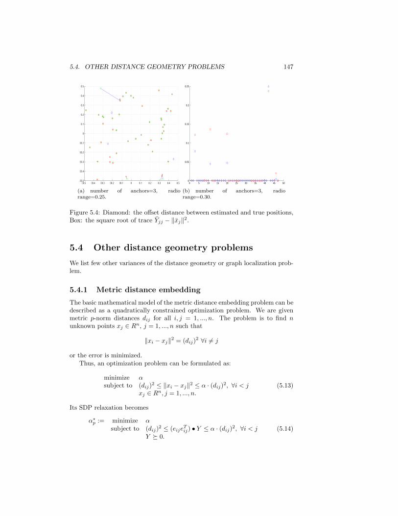
5.4. OTHER DISTANCE GEOMETRY PROBLEMS 147

−0.5 −0.4 −0.3 −0.2 −0.1 0 0.1 0.2 0.3 0.4 0.5−0.5

−0.4

−0.3

−0.2

−0.1

0

0.1

0.2

0.3

0.4

0.5

(a) number of anchors=3, radiorange=0.25.

0 5 10 15 20 25 30 35 40 45 500

0.05

0.1

0.15

0.2

0.25

(b) number of anchors=3, radiorange=0.30.

Figure 5.4: Diamond: the offset distance between estimated and true positions,Box: the square root of trace Yjj − ‖xj‖2.

5.4 Other distance geometry problems

We list few other variances of the distance geometry or graph localization prob-lem.

5.4.1 Metric distance embedding

The basic mathematical model of the metric distance embedding problem can bedescribed as a quadratically constrained optimization problem. We are givenmetric p-norm distances dij for all i, j = 1, ..., n. The problem is to find nunknown points xj ∈ Rn, j = 1, ..., n such that

‖xi − xj‖2 = (dij)2 ∀i 6= j

or the error is minimized.Thus, an optimization problem can be formulated as:

minimize αsubject to (dij)

2 ≤ ‖xi − xj‖2 ≤ α · (dij)2, ∀i < jxj ∈ Rn, j = 1, ..., n.

(5.13)

Its SDP relaxation becomes

α∗p := minimize αsubject to (dij)

2 ≤ (eijeTij) • Y ≤ α · (dij)2, ∀i < j

Y 0.(5.14)


Again

eij = (0, ..., 1, ...,−1, ...)T .

The SDP dual is

α∗p := Maximize∑i<j uij(dij)

2

Subject to 0 ∑i,j(uij − vij)eijeTij ,∑

i,j vij(dij)2 = 1

uij , vij ≥ 0.

Result and questions:

• α∗2 = 1, and α∗p ≤ O(log n) for all p.

• Reduce Y ∗’s rank to O(log n) for α∗2 = 1 + ε.

• rank ≤ O(log n) for α∗p ≤ O(log n) for all p.

• Better bound for α∗1?

5.4.2 Molecular confirmation

The basic mathematical model of the molecular confirmation problem can bedescribed as a quadratically constrained optimization problem as well. For apair of (i, j) ∈ N , we are given Euclidean distance upper bound dij and lowerbound dij between points i and j, the problem is to find Y such that

(dij)2 ≤ (eije

Tij) • Y ≤ (dij)

2, ∀i < j ∈ N .

Furthermore, it is desired to find other missing dij such that the Euclideandistance matrix can be completed.

The progem can be formulated as an SDP:

minimize I • Ysubject to (dij)

2 ≤ (eijeTij) • Y ≤ (dij)

2, ∀i < j ∈ NY 0.

(5.15)

5.4.3 Euclidean ball parking

The Euclidean ball packing problem is an old mathematical geometry problemwith plenty modern applications in Bio-X and chemical structures. It is a specialcase of the Euclidean distance geometry problem, say d = 3, xj ∈ R3 is theunknown position of the center of ball j, dij = ∞ and dij = ri + rj , where riand rj are the radii of balls i and j, respectively; and Ω represents a convexcontainer where the balls should be packed.

5.4. OTHER DISTANCE GEOMETRY PROBLEMS 149

Say that we want to pack n balls in a box with width and length equal 2Rand like to minimize the height of the box, we can formulate it as

minimize αsubject to ‖xi − xj‖2 ≥ (ri + rj)

2, ∀i 6= j,−R+ rj ≤ xj(1) ≤ R− rj , ∀j,−R+ rj ≤ xj(2) ≤ R− rj , ∀j,rj ≤ xj(3) ≤ α− rj , ∀j,

(5.16)

The first constraint tells that the distance between any two balls should begreater than or equal to the sum of the two balls’ radii, the second says thatthe first coordinate of xj is within the width constraint and the third is for thelength requirement, and the fourth indicates that the ball center has to be aboverj from the bottom and its height is below α− rj where α is to be minimized.

5.4.4 Data dimensionality reduction

Given P , a data point set of p1, ..., pn ∈ Rd, a fundamental question is how toembed P into Q of q1, ..., qn ∈ Rk, where k d, such that qjs keep all essentialinformation of P , such as the norms, distances and angles between pjs. In otherwords, find a d−k-dimension subspace such that the projections of pjs onto thesubspace has a minimal “information loss.” We believe that this problem canbe posted as an Euclidean distance geometry problem

Lk := minimize α

subject to∑n−ki=1 ((pl)

Txi)2 ≤ α, ∀l,∑n−k

i=1 ((pl − pm)Txi)2 ≤ α, ∀l < m,

‖xi‖2 = 1, i = 1, ..., n− k, (xh)Txi = 0, ∀h < i.(5.17)

Here, x1, ..., xn−k represent the n−k orthogonal bases of a n−k-dimension sub-space. Thus, (pTl xi; ...; p

Tl xn−k) represents the projection of pl onto the n − k

subspace. After the problem being solved and the subspace is found, the projec-tions of pls onto the complement k-dimension subspace must have all remaininginformation of pls. In fact, the model without pair-wise distance constraintsis called the minimum radius problem, which is a fundamental computationalgeometry and statistics problem.

Assume that x1, x2, · · · , xn−k ∈ Rd are the optimal solution of (5.17). Thenone can easily verify that the matrix Y = x1x

T1 + x2x

T2 + · · · + xn−kx

Tn−k is a

feasible solution for the following SDP model:

α∗k := minimize αsubject to pTl Y pl ≤ α, ∀l,

(pl − pm)TY (pl − pm) ≤ α, ∀l < m,tr(Y ) = n− k, I − Y 0, Y 0.

(5.18)

It follows that α∗k ≤ Rk(P )2. Then, we can design a rounding procedure toround Y , a solution to (5.18), into orthogonal n − k bases and prove theirquality.


Theorem 5.9 We can computed in polynomial time, a (n − k)-subspace suchthat, with probability at least 1 − 2

n , its projected value of (5.17) is at most12 log(n) of the minimal one.

5.5 A special case: The k-radius of P

The outer-radius, Rk(P ), is the minimum of the Euclidean radius of P projectedonto a k-dimensional subspace. Computing the minimal radius is a fundamentalproblem in computational convexity with applications in global optimization,data mining, statistics and clustering, and has received considerable attentionin the computational geometry literature [62, 155].

The square of Rk(P ) can be defined by the optimal value of the followingEuclidean distance minimization:

Rk(P )2 := minimize α

subject to∑ki=1((pl)

Txi)2 ≤ α, ∀pl ∈ P,

‖xi‖2 = 1, i = 1, ..., k, (xi)Txj = 0, ∀i 6= j ≤ k.

(5.19)This leads to the following SDP relaxation:

α∗k := minimize αsubject to tr(plp

Tl X) ≤ α, ∀pl ∈ P,

tr(X) = k, I −X 0, X 0.(5.20)

It follows that α∗k ≤ Rk(P )2.

Lemma 5.10 There exists an integer r ≥ k such that we can compute, inpolynomial time, r nonnegative reals λ1, λ2, · · · , λr and r orthogonal unit vectorsv1, v2, · · · , vr such that

(i).∑ri=1 λi = k.

(ii). max1≤i≤r λi ≤ 1.

(iii).∑ri=1 λi〈p, vi〉2 ≤ Rk(P )2, for any p ∈ P .

Proof. We solve the semidefinte program (5.20), and let X∗ be an optimalsolution of (5.20). We claim that the rank of X∗, say r, is at least k. This followsfrom the fact that tr(X∗) = k and I − X∗ 0. In other words, tr(X∗) = kimplies that the sum of the eigenvalues of X∗ is equal to k, and I − X∗ 0implies that the all eigenvalues are less than or equal to 1. Therefore, X∗ hasat least k non-zero eigenvalues, which implies that the rank of X∗ is at leastk. Let λ1, λ2, · · · , λr be the r nonnegative eigenvalues and v1, v2, · · · , vr be thecorresponding eigenvectors. Then we have

∑ri=1 λi = k and max1≤i≤r λi ≤ 1.

Furthermore, for any p ∈ P ,r∑i=1

λi〈p, vi〉2 = tr(ppTr∑i=1

λivivTi ) = tr(ppTX∗) ≤ α∗k ≤ Rk(P )2.

5.5. A SPECIAL CASE: THE K-RADIUS OF P 151

5.5.1 Deterministic First Rounding

In this section, we prove a lemma concerning how to deterministically group theeigenvalues and their eigenvectors. The proof of the lemma is elementary but itplays an important role for proving our main result.

Lemma 5.11 The index set 1, 2, · · · , r can be partitioned into k sets I1, I2, · · · , Iksuch that

(i). ∪ki=1Ii = 1, 2, · · · , r, and for any i 6= j, Ii ∩ Ij = ∅.

(ii). For any i : 1 ≤ i ≤ k,∑j∈Ii λj ≥

12 .

Proof. Recall that∑rj=1 λj = k and 0 ≤ λj ≤ 1 for all j. Without

loss of generality, we can assume that λ1 ≥ λ2 ≥ · · · ≥ λr. Our partitioningalgorithm is the same as the Longest-Processing-Time heuristic algorithm forparallel machine scheduling problem. The algorithm works as follows:

STEP 1. For i = 1, 2, · · · , k, set Ii = ∅ and let Li = 0. Let I = 1, 2, · · · , r.STPE 2. While I 6= ∅

choose j from I with the smallest index;choose set i with the smallest value Li;Let Ii := Ii ∪ j, Li := Li + λj and I := I − j.

It is clear that when the algorithm stops, the sets I1, I2, · · · , Ik satisfy con-dition (i). Now we prove condition (2) by contradiction. Assume that thereexists some t such that

∑j∈It λj <

12 .

We now claim that, for all i,∑j∈Ii λj ≤ 1. Otherwise, suppose

∑j∈It′

λj > 1

for some t′. Note that λj ≤ 1 for every j and thus there are at least twoeigenvalues are assigned to It′ . Denote the last eigenvalue by λs′ . It followsthat

∑j∈It′

λj − λs′ =∑j∈It′\s′

λj ≤∑j∈It λj since, otherwise, we would

have not assigned λs′ to It′ in the algorithm. However, since∑j∈It λj <

12 , we

must have∑j∈It′

λj−λs′ =∑j∈It′\s′

λj <12 . Thus, λs′ >

∑j∈It′

λj− 12 >

12 .

This is impossible since λs′ is the last eigenvalue assigned to It′ , which impliesλs′ ≤ λj for every j ∈ It′ , and we have already proved that there must exist anl such that s′ 6= l ∈ It′ and λl ≤

∑j∈It′\s′

λj <12 . Therefore,

∑j∈Ii λj ≤ 1

for all i, and in particular∑j∈It λj <

12 . It follows that

∑ki=1

∑j∈Ii λj < k.

However, we know that, by condition (i),∑ki=1

∑j∈Ii λj =

∑rj=1 λj = k. This

results a contradiction. Therefore, such t does not exists and we have provedcondition (ii).

Notice that the running time of the partitioning algorithm is bounded byO(r · k). An alternative way of partitioning the eigenvalues is the following:First, put the eigenvalues that are greater than or equal to 1/2 into distinctsubsets. If the number of such eigenvalues, say l, is not less than k, then we aredone. Otherwise, arbitrarily put the remaining eigenvalues into k − l subsetssuch that the sum of eigenvalues in each subset is greater than or equal to 1/2.This method is suggested by an anonymous referee.


5.5.2 Randomized Second Rounding

Assume now that we have found I1, I2, · · · , Ik. Then our next randomizedrounding procedure works as follows.

STEP 1. Generate a r dimensional random vector φ such that each entry ofφ takes value, independently, −1 or 1 with probability 1

2 each way.

STEP 2. For i = 1, 2, · · · , k, let

xi =

∑j∈Ii φj

√λj · vj√∑

j∈Ii λj.

The following Lemmas show that x1, x2, · · · , xk form a feasible solution forthe original problem. In other words, they are k orthogonal unit vectors.

Lemma 5.12 For i = 1, 2, · · · , k, ‖xi‖ = 1.

Proof. Recall that 〈vl, vj〉 = 0 for any l 6= j and ‖vj‖ = 1. By definition,

‖xi‖2 = 〈xi, xi〉

=

⟨∑j∈Ii φj

√λjvj√∑

j∈Ii λj,

∑j∈Ii φj

√λjvj√∑

j∈Ii λj

⟩

=1∑

j∈Ii λj

⟨∑j∈Ii

φj√λjvj ,

∑j∈Ii

φj√λjvj

⟩

=1∑

j∈Ii λj

∑j∈Ii

〈φj√λjvj , φj

√λjvj〉

=1∑

j∈Ii λj

∑j∈Ii

‖φj√λjvj‖2

=1∑

j∈Ii λj

∑j∈Ii

(φj)2λj‖vj‖2

=1∑

j∈Ii λj

∑j∈Ii

λj

= 1

Lemma 5.13 If s 6= t then 〈xs, xt〉 = 0.

5.5. A SPECIAL CASE: THE K-RADIUS OF P 153

Proof. The proof is similar as that of Lemma 5.12.

〈xs, xt〉

=

⟨∑j∈Is φj

√λjvj√∑

j∈Is λj,

∑j∈It φj

√λjvj√∑

j∈It λj

⟩

=1√∑

j∈Is λj ·∑j∈It λj

⟨∑j∈Is

φj√λjvj ,

∑j∈It

φj√λjvj

⟩= 0.

The last equality holds since for any j ∈ Is and l ∈ It, 〈vj , vl〉 = 0.

Now we establish a bound on the performance of our algorithm. First, let usintroduce Bernstein’s Theorem (see, e.g., [240]), which is a form of the ChernoffBound.

Lemma 5.14 Let φ be a random vector whose entries are independent andeither 1 or −1 with probability .5 each way. Then, for any vector e and β > 0,

prob〈φ, e〉2 > β‖e‖2 < 2 · exp(−β2

).

Let Cip =∑j∈Ii λj〈p, vj〉

2. Then we have

Lemma 5.15 For each i = 1, 2, · · · , k and each p ∈ P , we have

prob〈p, xi〉2 > 12 log(n) · Cip <2

n3.

Proof. Given i and p, define a |Ii| dimensional vector e such that its entries are√λj〈p, vj〉, j ∈ Ii, respectively. Furthermore, we define the vector φ|Ii whose

entries are those of φ with indices in Ii. First notice that

‖e‖2 =∑j∈Ii

(√λj〈p, vj〉)2 =

∑j∈Ii

λj · 〈p, vj〉2 = Cip.


On the other hand,

〈p, xi〉2

=

⟨p,

∑j∈Ii

√λjvjφj√∑

j∈Ii λj

⟩2

=1∑

j∈Ii λj

⟨p,∑j∈Ii

√λjvjφj

⟩2

≤ 2

⟨p,∑j∈Ii

√λjvjφj

⟩2

(since∑j∈Ii

λj ≥1

2)

= 2

∑j∈Ii

√λjφj〈p, vj〉

2

= 2 〈φ|Ii , e〉2

Thus

prob〈p, xi〉2 > 12 log(n)Cip ≤ prob〈φ|Ii , e〉2 > 6 log(n)‖e‖2.

Therefore, the conclusion of the lemma follows by using Lemma 5.14 and byletting β = 6 log(n).

Theorem 5.16 We can computed in polynomial time, a (d− k)-flat such that,with probability at least 1 − 2

n , the distance between any point p ∈ P and F is

at most√

12 log(n) ·Rk(P ).

Proof. For given i = 1, 2, · · · , k and p ∈ P , consider the event

Bip = φ|〈p, xi〉2 > 12 log(n) · Cip

and B = ∪i,pBip. The probability that the event B happens is bounded by∑i,p

prob〈p, xi〉2 > 12 log(n) · Cip <2kn

n3≤ 2

n.

If B does not happen, then for any i and p,

〈p, xi〉2 ≤ 12 log(n) · Cip.

Therefore, for each p ∈ P ,

k∑i=1

〈p, xi〉2 ≤ 12 log(n)

k∑i=1

Cip ≤ 12 log(n) ·Rk(P )2.

The last inequality follows from Lemma 5.10. This completes the proof bytaking F as the flat which is orthogonal to the vectors x1, x2, · · · , xk.

5.6. DISTRIBUTED SDP COMPUTING 155

5.6 Distributed SDP computing

The SDP problems presented in this chapter can be solved in a distributed fash-ion which has not been studied before. Here we describe an iterative distributedSDP computation scheme to for sensor network localization. We first partitionthe anchors into many clusters according to their physical positions, and assignsome sensors into these clusters if a sensor has a direct connection to one of theanchors. We then solve semidefinite programs independently at each cluster,and fix those sensors’ positions which have high accuracy measures accordingthe SDP computation. These positioned sensors become “ghost anchors” andare used to decide the remaining un-positioned sensors. The distributed schemethen repeats. A round of the distributed computation method is straightforwardand intuitive:

1. Partition the anchors into a number of clusters according to their geo-graphical positions. In our implementation, we partition the entire sensorarea into a number of equal-sized squares and those anchors in a samesquare form a regional cluster.

2. Each (unpositioned) sensor sees if it has a direct connection to an anchor(within the communication range to an anchor). If it does, it becomes anunknown sensor point in the cluster to which the anchor belongs. Notethat a sensor may be assigned into multiple clusters and some sensors arenot assigned into any cluster.

3. For each cluster of anchors and unknown sensors, formulate the errorminimization problem for that cluster, and solve the resulting SDP modelif the number of anchors is more than 2. Typically, each cluster has lessthan 100 sensors and the model can be solved efficiently.

4. After solving each SDP model, check the individual trace (5.7) for eachunknown sensor in the model. If it is below a predetermined small tol-erance, label the sensor as positioned and its estimation xj becomes an“ anchor”. If a sensor is assigned in multiple clusters, we choose the xjthat has the smallest individual trace. This is done so as to choose thebest estimation of the particular sensor from the estimations provided bysolving the different clusters.

5. Consider positioned sensors as anchors and return to Step 1 to start thenext round of estimation.

Note that the solution of the SDP problem in each cluster can be carriedout at the cluster level so that the computation is highly distributive. The onlyinformation that needs to be passed among the neighboring clusters is which ofthe unknown sensors become positioned after a round of SDP solutions.

In solving the SDP model for each cluster, even if the number of sensors isbelow 100, the total number of constraints could be in the range of thousands.


However, many of those ”bounding away” constraints, i.e., the constraints be-tween two remote points, are inactive or redundant at the optimal solution.Therefore, we adapt an iterative active constraint generation method. First,we solve the problem including only partial equality constraints and completelyignoring the bounding-away inequality constraints to obtain a solution. Sec-ondly we verify the equality and inequality constraints and add those violatedat the current solution into the model, and then resolve it with a “warm-start”solution. We can repeat this process until all of the constraints are satisfied.Typically, only about O(n + m) constraints are active at the final solution sothat the total number of constraints in the model can be controlled at O(n+m).

5.6.1 Preliminary computational and simulation results

Simulations were performed on networks of 2, 000 to 4, 000 sensor points whichare randomly generated in a square region of [−.5 .5] × [−.5 .5]. We generallyselect the first 5−10% of the points as anchors, that is, anchors are also uniformlydistributed in the same random manner. The tolerance for labeling a sensor aspositioned is set at 0.01 · (1 + noisyfactor) · radiorange. One simulation solvesa network localization with 4, 000 sensors, where the entire sensor region ispartitioned into 10× 10 equal-sized squares, that is, 100 clusters, and the radiorange is set at .035. The total solution time for the five round computation onthe single Pentium 1.2 GHz and 500 MB PC, excluding computing dij , is aboutfour minutes using DSDP2.0. The final solution is ploted in Figure 3.

It is usually the outlying sensors at the boundary or the sensors which do nothave many anchors within the radio range that are not estimated in the initialstages of the method. Gradually, as the number of well estimated sensors or’ghost’ anchors grows, more and more of these points are positioned. We havealso estimated the same 4, 000 network using noisy data. It is noted that theerroneous points are isolated within particular regions. This clearly indicatesthat the clustering approach prevents the propagation of errors to other clusters.We feel that our distributed computation techlogy is promising for solving veryvery large scale distance geometry related problems.

5.7 Notes

The distance geometry problem and its variants arise from applications invarious areas, such as molecular conformation, dimensionality reduction, Eu-clidean ball packing, and more recently, wireless sensor network localization[5, 53, 81, 161, 271, 275]. In the sensor networks setting, the vertices of G cor-respond to sensors, the edges of G correspond to communication links, and theweights correspond to distances. Furthermore, the vertices are partitioned intotwo sets – one is the anchors, whose exact positions are known (via GPS, forexample); and the other is the sensors, whose positions are unknown. The goalis to determine the positions of all the sensors. We shall refer to this problemas the Sensor Network Localization problem. Note that we can view the Sensor

5.7. NOTES 157

−0.1 0 0.1 0.2 0.3 0.4 0.5

−0.4

−0.3

−0.2

−0.1

0

0.1

0.2

0.3

0.4

0.5

Figure 5.5: Third and final round position estimations in the 4, 000 sensornetwork, noisy-factor=0, radio-range=0.045, and the number of clusters=100.


Network Localization problem as a variant of the Graph Realization problem inwhich a subset of the vertices are constrained to be in certain positions.

In many sensor networks applications, sensors collect data that are location–dependent. Thus, another related question is whether the given instance hasa unique realization in the required dimension (say, in R2). Indeed, mostof the previous works on the Sensor Network Localization problem fall intotwo categories – one deals with computing a realization of a given instance[53, 81, 91, 161, 270, 271, 272, 275], and the other deals with determiningwhether a given instance has a unique realization in Rd using graph rigidity[91, 139]. It is interesting to note that from an algorithmic viewpoint, thetwo problems above have very different characteristics. Under certain non–degeneracy assumptions, the question of whether a given instance has a uniquerealization on the plane can be decided efficiently [169], while the problem ofcomputing a realization on the plane is NP–complete in general, even if the giveninstance has a unique realization on the plane [25]. Thus, it is not surprisingthat all the aforementioned heuristics for computing a realization of a given in-stance do not guarantee to find it in the required dimension. On another front,there has been attempts to characterize families of graphs that admit polyno-mial time algorithms for computing a realization in the required dimension. Forinstance, Eren et. al. [91] have shown that the family of trilateration graphs hassuch property. (A graph is a trilateration graph in dimension d if there existsan ordering of the vertices 1, . . . , d+ 1, d+ 2, . . . , n such that (i) the first d+ 1vertices form a complete graph, and (ii) each vertex j > d+ 1 has at least d+ 1edges to vertices earlier in the sequence.) However, the question of whetherthere exist larger families of graphs with such property is open.

We should mention here that various researchers have used SDP to studythe distance geometry problem (or its variants) before. For instance, Barvinok[35, 36] has studied this problem in the context of quadratic maps and usedSDP theory to analyze the possible dimensions of the realization. Alfakih andWolkowicz [6, 7] have related this problem to the Euclidean Distance MatrixCompletion problem and obtained an SDP formulation for the former. More-over, Alfakih has obtained a characterization of rigid graphs in [3] using Eu-clidean distance matrices and has studied some of the computational aspects ofsuch characterization in [4] using SDP. However, these papers mostly addressedthe question of realizability of the input graph, and the analyses of their SDPmodels only guarantee that they will find a realization whose dimension lieswithin a certain range. Thus, these models are not quite suitable for our appli-cation. In contrast, our analysis takes advantage of the presence of anchors andgives a condition which guarantees that our SDP model will find a realizationin the required dimension. We remark that SDP has also been used to computeand analyze distance geometry problems where the realization is allowed to havea certain amount of distortion in the distances [37, 205]. Again, these meth-ods can only guarantee to find a realization that lies in a range of dimensions.Thus, it would be interesting to extend our method to compute low–distortionrealizations in a given dimension. For some related work in this direction, see,e.g., [28].

5.8. EXERCISES 159

The SDP models were first used by [65, 66] for the ad hoc wireless sensornetwork localization, and the results described here were based on their work.

The result on the radii of point sets is due to [342], which improves the ratioof [320] by a factor of O(

√log d) that could be as large as O(

√log n). This ratio

also matches the previously best known ratio for approximating the special caseR1(P ) of [240], the width of point set P .

5.8 Exercises

5.1 Find the SDP relaxation to the following minimization problem


(αij)2 +

∑k,j∈Na

(αkj)2

subject to ‖xi − xj‖2 = (dij)2 + αij , ∀ (i, j) ∈ Nx, i < j,

‖ak − xj‖2 = (dkj)2 + αkj , for (k, j) ∈ Na,

‖xi − xj‖2 ≥ R2, for the rest i < j,‖ak − xj‖2 ≥ R2, for the rest k, j;

and interpret the objective function.

5.2 Find the SDP relaxation to the following minimization problem


(αij)2 +

∑k,j∈Na

(αkj)2

subject to ‖xi − xj‖ = dij + αij , ∀ (i, j) ∈ Nx, i < j,

‖ak − xj‖ = dkj + αkj , for (k, j) ∈ Na,‖xi − xj‖2 ≥ R2, for the rest i < j,‖ak − xj‖2 ≥ R2, for the rest k, j;

and interpret the objective function.

5.3 The Un-Folding Problem: with the same notions, consider the problem

maximize∑i ‖xi‖2

subject to ‖ak − xj‖2 = d2kj ∀ (k, j) ∈ Na

‖xi − xj‖2 = d2ij ∀ (i, j) ∈ Nx

(5.21)

Find the SDP relaxation and its dual, and explain what they are.

5.4 Given one sensor and three anchors in R2, and let the three distances fromthe sensor to three anchors are given. Show that the graph is stronly localizableif and only if the sensor’s position lies in the liner space of the three anchors’positions.

5.5 Prove that the graphs depicted in Figures 5.2(a) and 5.2(b) are stronglylocalizable.

5.6 Suppose for the angle of two edges joint at a point is known. How to inco-porate this information in the SDP relaxation of the distance geometry problem?


Chapter 6

SDP for RobustOptimization

6.1 Robust Optimization

Consider an optimization problem

Minimize f(x, ξ)(OPT)

Subject to F (x, ξ) ∈ K ⊂ Rm.(6.1)

where ξ is the data of the problem and x ∈ Rn is the decision vector, and K isa convex cone.

For deterministic optimization, we assume ξ is known and fixed. In reality,ξ may not be certain.

• Knowledge of ξ belonging to a given uncertain set U .

• The constraints must be satisfied for every ξ in the uncertain set U .

• Optimal solution must give the best guaranteed value of supξ∈U f(x, ξ).

This leads to the so-called robust counterpart:

Minimize supξ∈U f(x, ξ)(ROPT)

Subject to F (x, ξ) ∈ K for all ξ ∈ U.(6.2)

Other methods dealing with data uncertainty include:

161

162 CHAPTER 6. SDP FOR ROBUST OPTIMIZATION

6.1.1 Stochastic Method

Minimize Eξ[f(x, ξ)](EOPT)

Subject to Eξ[F (x, ξ)] ∈ K.

6.1.2 Sampling Method

Minimize z(SOPT)

Subject to F (x, ξk) ∈ K

f(x, ξk) ≤ zfor large sxamples ξk ∈ U.

This problem may be a semin-infinite programming problem.

6.2 Robust Quadratic Optimization

Minimize qTx(EQP)

Subject to ‖Ax‖2 ≤ 1.(6.3)

Here, vector q ∈ Rn and A ∈ Rm×n; and ‖.‖ is the Euclidean norm.

6.2.1 Ellipsoid uncertainty

Let A be uncertain and

A = A0 +

k∑j=1

ujAj | uTu ≤ 1.

Minimize qTx(REQP)

Subject to ‖(A0 +∑kj=1 ujA

j)x‖ ≤ 1 ∀uTu ≤ 1.

The problem can be rewritten as

Minimize qTx(REQP)

Subject to ‖(A0 +∑kj=1 ujA

j)x‖2 ≤ 1 ∀uTu ≤ 1.

LetF (x) = (A0x, A1x, · · · Akx).

6.2. ROBUST QUADRATIC OPTIMIZATION 163

Then

‖(A0 +

k∑j=1

ujAj)x‖2 =

(1u

)TF (x)TF (x)

(1u

)The problem becomes

Minimize qTx(REQP)

Subject to

(1u

)T ((1 00 0

)− F (x)TF (x)

)(1u

)≥ 0

∀(

1u

)T (1 00 −I

)(1u

)≥ 0.

6.2.2 S-Lemma

Lemma 6.1 Let P and Q be two symmetric matrices such that there exists u0

satisfying (u0)TPu0 > 0. Then the implication that

uTPu ≥ 0⇒ uTQu ≥ 0

holds true if and only if there exists λ ≥ 0 such that

Q λP.

From the lemma, we immediately see(1u

)T ((1 00 0

)− F (x)TF (x)

)(1u

)≥ 0

∀(

1u

)T (1 00 −I

)(1u

)≥ 0

if and only if there is a λ ≥ 0 such that(1 00 0

)− F (x)TF (x) λ

(1 00 −I

).

This is equivalent to (1 00 0

)+ λ

(−1 00 I

)F (x)T

F (x) I

0

which is a SDP constraint since F (x) is linear in x. Here we have used anothertechnical lemma

Lemma 6.2 Let P a symmetric matrix and A be a rectangle matrix. Then

P −ATA 0

if and only if (P AT

A I

) 0.


6.2.3 SDP for Robust QP

Consider λ and x as variables, REQP finally becomes a SDP problem:

Minimize qTx(REQP)

Subject to

(1− λ 0

0 λI

)F (x)T

F (x) I

0.

6.3 General Robust Quadratic Optimization

Minimize qTx(EQP)

Subject to −xTATAx+ 2bTx+ γ ≥ 0.(6.4)

Here, vector q, b ∈ Rn and and A ∈ Rm×n.



(A, b, γ) = (A0, b0, γ0) +

k∑j=1

uj(Aj , bj , γj)| uTu ≤ 1.

Minimize qTx(REQP)

Subject to −xTATAx+ 2bTx+ γ ≥ 0 ∀uTu ≤ 1.

Let again

F (x) = (A0x, A1x, · · · Akx).

Then

−xTATAx+ 2bTx+ γ =

(1u

)T

γ0 + 2xT b0 γ1/2 + xT b1 · · · γk/2 + xT bk

γ1/2 + xT b1 0 · · · 0· · · · · · · · · · · ·

γk/2 + xT bk 0 · · · 0

− F (x)TF (x)

( 1u

).

6.4. MORE ROBUST QUADRATIC OPTIMIZATION 165

6.3.2 SDP formulation

From the S-lemma, we immediately see if and only if there is λ ≥ 0 such thatγ0 + 2xT b0 γ1/2 + xT b1 · · · γk/2 + xT bk

γ1/2 + xT b1 0 · · · 0· · · · · · · · · · · ·

γk/2 + xT bk 0 · · · 0

−F (x)TF (x)) λ(

1 00 −I

);

which is is equivalent to

γ0 + 2xT b0 γ1/2 + xT b1 · · · γk/2 + xT bk

γ1/2 + xT b1 0 · · · 0· · · · · · · · · · · ·

γk/2 + xT bk 0 · · · 0

+ λ

(−1 00 I

)F (x)T

F (x) I

0.

which is a SDP constraint since the matrix is linear in x.Consider λ and x as variables, REQP finally becomes a SDP problem:

Minimize qTx(REQP)

Subject to

γ0 + 2xT b0 − λ γ1/2 + xT b1 · · · γk/2 + xT bk

γ1/2 + xT b1 λ · · · 0· · · · · · · · · · · ·

γk/2 + xT bk 0 · · · λ

F (x)T

F (x) I

0.

6.4 More Robust Quadratic Optimization

Minimize qTx(EQP)

Subject to −xTATi Aix+ 2bTi x+ γi ≥ 0 i = 1, ..., t.(6.5)

Here, vector q, bi ∈ Rn and and Ai ∈ Rm×n.



(Ai, bi, γi) = (A0i , b

0i , γ

0i ) +

k∑j=1

uj(Aji , b

ji , γ

ji )| u

Tu ≤ 1.

Minimize qTx(REQP)

Subject to −xTATi Aix+ 2bTi x+ γi ≥ 0, i = 1, ..., t, ∀uTu ≤ 1.


6.4.2 SDP formulation

Let again

Fi(x) = (A0ix, A

1ix, · · · Aki x).

Consider λi, i = 1, ..., t, and x as variables, REQP finally becomes a SDPproblem:

Min qTx

s.t.

γ0i + 2xT b0i − λi γ1

i /2 + xT b1i · · · γki /2 + xT bkiγ1i /2 + xT b1i λi · · · 0· · · · · · · · · · · ·

γki /2 + xT bki 0 · · · λi

Fi(x)T

Fi(x) I

0,

i = 1, ..., t.

6.5 Tool for Robust Optimization

Recall:Minimize supξ∈U f(x, ξ)

(ROPT)Subject to F (x, ξ) ≤ 0 for all ξ ∈ U.

(6.6)

Express

ξ = ξ(u) where u ∈ U .

Then,

supξ∈U

f(x, ξ) = supu∈U

f(x, ξ(u))

In convex cases, we represent

supu∈U

f(x, ξ(u))

by its conic dual problem and let the dual objective function be

φ(λ0, x)

where λ0 is the dual variables. The dual objective function is an upper boundon f(x, ξ(u)) so we could represent the problem by

Minimize φ(λ0, x)(ROPT)

Subject to F (x, ξ) ≤ 0 for all ξ ∈ U

dual constraints on λ0.

(6.7)

6.5. TOOL FOR ROBUST OPTIMIZATION 167

We handle the constraints in the exact same manner, and the problem be-comes

Minimize φ(λ0, x)(ROPT)

Subject to Φ(λ, x) ∈ C

dual constraints on λ0, λ,

(6.8)

where Φ(λ, x) is, component-wise, the dual objective function of

supu∈U

F (x, ξ(u)),

and C is a suitable cone.

6.5.1 Examples

ax+ b ≤ 0

where

(a, b) = (a0, b0) +

k∑i=1

ui(ai, bi)| u ∈ U .

Case of ‖u‖ ≤ 1:

maxu:‖u‖≤1

a0x+ b0 +

k∑i=1

ui(aix+ bi)

The dual is

Minimize λ

Subject to λ− (a0x+ b0) ≥√∑k

i=1(aix+ bi)2.

Thus, the robust constraint becomes

0 ≥ λ ≥ (a0x+ b0) +

√√√√ k∑i=1

(aix+ bi)2.

Case of ‖u‖∞ ≤ 1:

maxu:‖u‖∞≤1

a0x+ b0 +

k∑i=1

ui(aix+ bi)

The dual is

Minimize λ

Subject to λ− (a0x+ b0) ≥∑ki=1 |(aix+ bi)|.



0 ≥ λ ≥ (a0x+ b0) +

k∑i=1

|(aix+ bi)|.

Case of ‖u‖1 ≤ 1:

maxu:‖u‖1≤1

a0x+ b0 +

k∑i=1

ui(aix+ bi)

The dual is

Minimize λ

Subject to λ− (a0x+ b0) ≥ maxi|(aix+ bi)|.


0 ≥ λ ≥ (a0x+ b0) + maxi|(aix+ bi)|.

6.6 Applications

6.6.1 Robust Linear Least Squares

Minimize ‖Ay − c‖2y ∈ Y.

If the data (A, c) are from the set

(A, c) = (A0, c0) +

k∑i=1

ui(Ai, ci)| ‖u‖ ≤ 1,

the robust counter part can be drawn from the earlier disscusion, since theoriginal problem is a convex QP problem.

6.6.2 Heat dissipation problem

Consider an electric circuit represented as a connected oriented graph Γ withN arcs, each of which possesses a given conductance sij . Assuming that thearcs of the circuit are charged with external voltages y and internal voltages v.These voltages induce currents in the circuit; as a result, the circuit dissipatesheat. According to Kirchoff’s laws, the heat is given by

H = minv∈Rm

(Qv + Py)TS(Qv + Py),

where Q and P are some matrices given by the topology of the circuit, m is thenumber of nodes of the circuit, and S is N ×N diagonal matrix with sij as itsdiagonal entries.

6.7. EXERCISES 169

The problem is to choose y such that

miny∈Y

[minv∈Rm

(Qv + Py)TS(Qv + Py)

],

where Y is a convex set.Now if

S = S(u) = S0 +

k∑i=1

uiSi| ‖u‖ ≤ 1,

we have a robust optimization counterpart:

miny∈Y

maxu∈U

[minv∈Rm

(Qv + Py)TS(u)(Qv + Py)

].

Since (Qu+Py)TS(u)(Qu+Py) is convex in (y, v) and linear in u, this problemis equivalent to

miny∈Y,v∈Rm

[maxu∈U

(Qv + Py)TS(u)(Qv + Py)

].

6.6.3 Portfolio optimization

Minimize xTV x

Subject to µTx ≥ α

eTx = 1.

Now V and µ may be uncertain, for example,

(V, µ) = (V 0, µ0) +

k∑i=1

ui(Vi, µi)| ‖u‖ ≤ 1.

The robust counterpart of the portfolio problem is

Minimize maxV ∈V [xTV x]

Subject to minµ∈S [µTx] ≥ α

eTx = 1

6.7 Exercises

6.1 Prove the S-lemma.

6.2 In the linear least squares problem, assume that

(A, c) = (A0, c0) +

k∑i=1

ui(Ai, ci)| ‖u‖ ≤ 1.


Construct the robust counterparts of the problem for three norms on u:

‖u‖2 ≤ 1, ‖u‖1 ≤ 1, and ‖u‖∞ ≤ 1.

6.3 In the Heat dissipation problem, assume that

S = S(u) = S0 +

k∑i=1

uiSi| ‖u‖ ≤ 1,

and si 0 for all i = 0, ..., k. Construct the robust counterparts of the problemfor three norms on u:

‖u‖2 ≤ 1, ‖u‖1 ≤ 1, and ‖u‖∞ ≤ 1.

6.4 In the portafolio optimization problem, assume that

(V, µ) = (V 0, µ0) +

k∑i=1

ui(Vi, µi)| ‖u‖ ≤ 1,

and V i 0 for all i = 0, ..., k. Construct the robust counterparts of the problemfor three norms on u:

‖u‖2 ≤ 1, ‖u‖1 ≤ 1, and ‖u‖∞ ≤ 1.

Chapter 7

SDP for QuantumComputation

7.1 Quantum Computation

Quantum Computation uses Quantum Mechanics to enhance computation power.First concrete result was developed for Integer Factorization by Shor in 1994;and then for Quantum search algorithm and space reduction by Grover in 1996.The field is closely linked to Quantum Information Theory and Statistics, Quan-tum Channels and Optimization.

To describe quantum mechanics, Hilbert sapces and linear operators aregenerally used. In this lecture, we restrict ourselves to finite-dimensional realvector spaces. In classical quantum physics, a quantum state, or a state, isa column vector v in the N -dimensional vector space RN with norm ||v||2 =√v · v = 1.

Nowadays, another formalism is widely accepted, in which a state is a postivesemidefinite symmetric matrix V with trace 1 that belongs to RN×N . A matrixof such property is called a density matrix. For example, a density matrix Vwith rank one can be represented as V = vvT , and Tr(V ) = 1. A density matrixof rank higher than 1 can be written as

V =

N∑i=1

λivivTi ,

where λi ≥ 0 for all i and∑i λi = 1.

A density matrix of rank 1 is called a pure sate, and a density matrix of rankhigher than 1 is called a mixed state. The state V is interpreted as a probalisticmixture of pure states viv

Ti with mixing probabilities λi.

171

172 CHAPTER 7. SDP FOR QUANTUM COMPUTATION

7.2 Completely Positive Map

The state of a system may change as time goes on.Given A1, A2, · · · , Ak, where Ai ∈ RM×N , such that

k∑i=1

AiATi = I,

trace-preserving complete positive (CP) map of V is

T (V ) =

k∑i=1

AiV ATi .

Note that T (V ) ∈ RM×M , so CP is a linear mapping that conveys quantumstates in RN×N to the states in RM×M . In quantum computing, the pure stateis in R2n

or N = 2n, called n-qubit. When n = 1, a unit orthogonal (1; 0) and(0; 1) represent the classical bits.

A measurement is described as a finite set of symmetric positive semidefinitematrices M1,M2, · · · ,Mk whose sum is an identity matrix, i.e.,

Mi 0, ∀i = 1, · · · , k, and

k∑i=1

Mi = I,

called Positive Operator-Valued Measures (POVM).Given the system in state V and a measurement M1,M2, · · · ,Mk per-

formed on the system, we obtain a random varible X with

Pr(X = l) = V •Ml, l = 1, · · · , k.

A fundamental problem is quantum detection theory is to find an optimalmeasurement for given mixed states.

Suppose we are given m states V1, V2, · · · , Vm with corresponding prior prob-abilities ξ1, ξ2, · · · , ξm. For a measurement M = M1, . . . ,Mk, we have

P (j|i) = Tr(ViMj).

Let cij(≥ 0) be the cost (penlaty) of taking a true state i to be j. Then theaverage cost is

C(M) =∑i,j

ξiP (j|i)cij =∑j

Tr

[(∑i

ξiVicij

)Mj

].

Let Wj =∑i ξiVicij , j = 1, . . . , k. The problem of minimizing the average

cost can be formulated as the following SDP:

Minimize∑kj=1 Tr(WjMj)

Subject to∑kj=1Mj = I,

Mj 0, j = 1, . . . , k.

7.3. CHANNEL CAPACITY PROBLEM 173

What is the dual?

Maximize∑kj=1 Tr(U)

Subject to Wj U, j = 1, . . . , k.

Thus, the optimality Condition becomes

Wi k∑j=1

MjWj =

k∑j=1

WjMj , i = 1, ..., k.

7.3 Channel Capacity Problem

A classical discrete memoryless channel consists of a set of input symbols A =a1, a2, . . . , am, a set of output symbols B = b1, b2, . . . , bn and a set of con-

ditional probabilities Vij = P (bj |ai) with

n∑j=1

Vij = 1, for i = 1, . . . ,m.

Therefore, V = Vij is a stochastic matrix, where Vij is the probabilitythat bj is received when ai is sent through the channel. The capacity C(V ) of achannel V , defined as the maximum of rates (speeds) at which information canbe transmitted reliably, is given by following theorem due to Shannon.

The classical channel coding theorem is modeled as:

C(V ) Maximize I(p, V )

Subject to∑mi=1 pi = 1, with p = pi

pi ≥ 0, i = 1, . . . ,m,

where

I(p, V ) =∑i

pi∑j

Vij logVij∑

k

pkVkj

The Kullback -Leibler divergence, defined as follows

D(q||r) =∑j

qj logqjrj,

is a measure of distance between two probability distributions q = (qj) andr = (rj), and plays an important role in information theory.

Then, the function I(p, V ) can be written in terms of the above Kullback-Leibler divergence

I(p, V ) =∑i

piD(Vi·||pV ),

where r = pV is a distribution defined by rj =∑i piVij . With a channgel V

fiexed, I(p, V ) is concave in p = (pi). Hence, the computatution of C(V ) is aconcave maximization problem with linear constraints.


A quantum memoryless channel consists of a set S1 of input states (or densitymatrices) in Rm×m, S2 of output states (or density matrices) in Rn×n, and aCP (map) Γ : S1 → S2. The capacity C(Γ) of a quantum channel Γ, definedto be the maximum of rates (speeds) at which reliable transmission of classicalinformation through the channel Γ is possible.

The Quantum channel coding theorem due to A. S. Holevo is modeled by

C(V ) Maximize I(λi, Xi,Γ)

Subject to Xi ∈ S1, i = 1, . . . , d∑di=1 λi = 1

λi ≥ 0, i = 1, . . . , d,

where d = n2, and

I(λi, Xi,Γ) =∑i

λiTr(Γ(Xi))[log Tr(Γ(Xi))− log Tr(Γ(X))

],

with X =∑i λiXi.

Observe that I(λi, Xi,Γ) can be written in terms of the quantum coun-terpart of the Kullback-Leibler divergence (often called relative entropy)

D(X||Y ) = Tr(X)[log Tr(X)− log Tr(Y )].

Once the ensemble X = Xi is fixed, I(λi, Xi,Γ) is a concave function inλ = λi. This is again a convex programming problem.

But, in general, I(λi, Xi,Γ) is neither convex nor concave in (λ,X).

7.4 Quantum Interactive Proof System

Interation Between Prover and Verifier.Consider two CP mappings: given A1, A2, · · · , Ak and B1, B2, · · · , Bl,

where Ai, Bi ∈ RM×N , such that

k∑i=1

AiATi = I and

l∑i=1

BiBTi = I,

Define

T1(V ) =

k∑i=1

AiV ATi

and

T2(V ) =

l∑i=1

BiV BTi .

7.5. NOTES 175

The question is, are there two states V1 and V2 such that

T1(V1) = T2(V2);

or for all V1 and V2

‖T1(V1)− T2(V2)‖ ≥ ε.

An SDP Formulation for this problem is

Minimize t

Subject to I • V1 = I • V2 = 1,

V1, V2 0T1(V1)− T2(V2) + t · I 0t · I − T1(V1) + T2(V2) 0.

7.5 Notes

7.6 Exercises


Chapter 8

Computational Issues

It is common to have a gap between a theoretical algorithm and its practicalimplementation: the theoretical algorithm makes sure that it works for all in-stances and never fails, while the practical implementation emphasizes averageperformance and uses many ad-hoc “tricks.” In this chapter we discuss sev-eral effective implementation techniques frequently used in interior-point linearprogramming software, such as the presolver process, the sparse linear systemsolver, the high-order predictor-corrector method, the homogeneous and self-dual method, and the optimal basis finder. Our goal is to provide additionaltheoretical justification for using these techniques and to explain their practicaleffectiveness.

8.1 Presolver

One way to eliminate data error and to improve solution efficiency in solvinglinear programs is called the “presolver”—a preliminary process to check thedata set (A, b, c) in order to detect inconsistency and to remove redundancy.This process could reduce the size of the problem as well, because users of manyLP problems likely introduce superfluous variables and redundant constraintsfor simplicity and convenience in model formulation.

In general, detecting all inconsistency and redundancy in an LP problem iscomputationally intractable. Therefore all presolvers use an arsenal of simpleinspection techniques. These techniques are applied repeatedly until the prob-lem cannot be reduced any further. Below, we briefly present the most commoninspection procedures.

177

178 CHAPTER 8. COMPUTATIONAL ISSUES

• Remove empty or all-zero rows and columns.

• Eliminate a fixed variable, the variable has a fixed value, from the problemby substitution.

• Remove duplicate constraints. Two constraints are said to be duplicateif they are identical up to a scalar multiplier. One of the duplicate con-straints is removed from the problem.

Remove duplicate columns. Two columns are said to be duplicate if theyare identical up to a scalar multiplier. (They make duplicate constraintsin the dual.)

• Remove linearly dependent constraints. The presence of linearly depen-dent rows in A may lead to serious numerical problems in an interior-pointmethods, since it implies a rank deficiency in the Newton equation system.

• Remove a singleton row (only one non-zero coefficient in the row) by con-struction of a simple variable bound. For example, if the ith constraint isin the form ai1x1 ≤ bi, we can convert it to x1 ≤ bi/ai1 or x1 ≥ bi/ai1,depending on the sign of ai1,

• Remove a free and singleton column (only one non-zero coefficient in thecolumn and the associated variable is free). For example, let free variablex1 appears only in the ith constraint. Then, x1 and the ith constraint canbe eliminated, while the optimal value of x1 can be recovered from theith constraint by substitution of the optimal solution of the remaining LPproblem.

A nonnegative but unbounded variable, say, 0 ≤ x1 < +∞ in singletoncolumn 1, can be used to generate a bound on dual variables yi. Namely,

ai1yi ≤ c1.

This inequality can be used, depending on the sign of ai1, to produce alower or upper bound on yi.

• Determine lower and upper limits for every constraint and detect infeasi-bility. For example, consider the ith (inequality) constraint∑

j

aijxj ≤ bi,

and let each variable xj lie on [0, uj ]. Then compute

bi =∑

j: aij<0

aijuj ≤ 0 and bi =∑

j: aij>0

aijuj ≥ 0. (8.1)

Thus, we must have

bi ≤∑j

aijxj ≤ bi. (8.2)

8.2. LINEAR SYSTEM SOLVER 179

If bi ≤ bi, then the ith constraint is redundant and can be removed. Ifbi > bI , then the problem is infeasible. If bi = bi, the i constraint be-comes equality and will force all involved variables take values at theirappropriate bounds.

The same technique can be applied to each of the dual constraints.

• Add implicit bound to a free primal variable. For example, suppose theith constraint is ∑

j

aijxj = bi,

where ai1 > 0, x1 is a free variable, and all other variables xj lie on [0, uj ].Then

x1 ≤

bi − ∑j 6=1: aij<0

aijuj

/ai1

and

x1 ≥

bi − ∑j 6=1: aij>0

aijuj

/ai1.

The same technique can be applied to a dual free variable.

• Improve the sparsity of A, i.e., reduce the non-zero elements in A. Wecould look for a nonsingular matrix M ∈ Rm×m such that the matrix MAis as sparse as possible. Primal constraints can in such case be replacedwith equivalent

MAx = Mb, (8.3)

which may be more suitable for an interior-point solver. Exact solutionof this sparsity problem is an NP-complete problem but efficient heuristicsusually produce satisfactory non-zero reduction in A.

The application of the above presolver techniques often results in impressivesize-reduction of an initial LP formulation. Thus, it is our hope that the reducedproblem obtained after the presolver can be solved faster. Once a solution isfound, it could be used to recover a complete primal and dual solution to theoriginal LP problem. This phase is called the postsolver.

8.2 Linear System Solver

The major work in a single iteration of all interior-point algorithms is to solve aset of linear equations, such as (3.38). It can be reduced to the so-called KKTsystem: (

D−2 AT

A 0

)(dx−dy

)=

(cb

), (8.4)


The diagonal matrix D varies in different interior-point methods. Mostgeneral purpose codes use direct methods to solve the KKT system. Two com-petitive direct methods are: the normal equation approach and the augmentedsystem approach. The former works with a smaller positive definite matrix, andthe latter requires factorization of a symmetric indefinite matrix. They all usevariants of the symmetric triangular LΛLT decomposition, where L is a lowertriangular matrix and Λ is a block diagonal matrix with blocks of dimension1 or 2. (The QR decomposition of A uses an orthogonal transformation andguarantees high accuracy, but it cannot be used in practice due to its costlyoperations.)

8.2.1 Solving normal equation

The normal equation approach further reduces (8.4) to the normal equation:

(AD2AT )dy = b−AD2c. (8.5)

An advantage of this approach is that it works with a positive definite matrixAD2AT if A has full row rank. Thus the Choleski decomposition of this matrixexists for any D and numerical stability is assured in the pivoting process.Moreover, the sparsity pattern in the decomposition is independent of the valueof D and hence it is invariant in all iterations. Consequently, once a goodsparsity preserving pivoting order is chosen, it can be used throughout the entireiterative process. This argument has been used to justify the application of thenormal equations approach in very first interior-point method implementation.

The success of the Choleski factorization depends on a pivoting order forpreserving sparsity in the Choleski factor L. Its goal is to find a permutationmatrix P such that the factor of PAD2ATPT is as sparse as possible. Inpractice, heuristics are used to find such a permutation or ordering. (Findingan optimal permutation is an NP-complete problem.) After an ordering is found,the data structure and indirect index addressing of L are setup. This is referredto as the symbolic phase because no numerical computation is involved.

Two heuristic orderings, minimum degree and the minimum local fill-in, areparticularly useful in implementing interior-point algorithms. They are both“local” or myopic, i.e. they select a pivot only from a set of currently bestcandidates.

Minimum degree ordering

Assume that, in the kth step of the Gaussian elimination, the ith column of theSchur complement contains di non-zero entries and its diagonal element becomesa pivot. The kth step of the elimination requires thus

li = (1/2)(di − 1)2, (8.6)

floating-point operations or flops to be executed.


In what follows, keep in your mind the fact that the decomposed matrixAD2AT is positive definite so the pivot choice can be limited to the diagonalelements. In fact, only this choice preserves symmetry.

Note that if the ith diagonal element becomes a pivot, li evaluates flops andgives an overestimate of the fill-ins, the new non-zeros created in the Schur com-plement, which can result from the current elimination step. Thus, the “best”pivot at step k, in terms of the number of flops required to complete the kthelimination step, is the one that minimizes di among all diagonal elements in theSchur complement. Interpreting the elimination process as the correspondingincidence graph elimination, one can see that this strategy chooses a node (di-agonal element) in the graph which has the minimum degree (di). This is howthe strategy is named. This ordering procedure can be implemented efficientlyboth in terms of time speed and storage requirement.

There is also an approximate minimum degree ordering available. Themethod is faster while generates the same quality ordering.

Minimum local fill-in ordering

In general, li of (8.6) considerably overestimates the number of fill-ins in thekth step of the Gaussian elimination, because it does not take into accountthe fact that in many positions of the predicted fill-ins, non-zero entries alreadyexist. It is possible that another pivot candidate, although may not minimize di,would produce least fill-ins in the remaining Schur complement. The minimumlocal fill-in ordering chooses such a pivot. Generally, the minimum local fill-inprocedure produces an ordering resulting in a sparser factorization but at ahigher cost, because it chooses the pivot that produces the minimum number offill-ins among all remaining pivot candidates.

Pros and cons

Solving the normal equation is proved to be a reliable approach to solutionsof most practical linear programs. However, it suffers two drawbacks. First,the normal equation behaves badly whenever a primal linear program containsfree variables. In order to transform such a problem to the standard form, afree variable is usually replaced with the difference of two nonnegative variables:x = x+−x−. Interior-point algorithms typically generate iterates in which bothx+ and x− converge to∞, although their difference is kept relatively close to theoptimal value of x. This results in a serious ill-condition in the normal matrixand a loss of accuracy in solving (8.5). A remedy used in many implementationsis to prevent excessive growth of x+ and x− by enforcing bounds on x+ and x−.

Second, a more serious drawback of the normal equation approach is that itlooses sparsity from the presence of dense columns in A. The reason is that asingle dense column in A with p non-zero elements creates a complete dense sub-matrix of size p× p in AD2AT after a symmetric row and column permutation.Special care has to be taken in this case.


Assume that

A = (AS , AD), (8.7)

where AS ∈ Rm×n−k is sparse and AD ∈ Rm×k is dense. Then, we need to treatAD separately. The most popular way in solving the normal equation employsthe Schur complement mechanism. It is based on separating the normal matrix

AD2AT = ASD2SA

TS + ADD

2DA

TD, (8.8)

into the presumably sparse part ASD2SA

TS and the significantly denser sym-

metric rank-k matrix ADD2DA

TD. A Choleski decomposition is computed for

the sparse part and the dense rank-k matrix is then updated by the Sherman-Morrison-Woodbury formula (see Exercise 1.1).

This method is not guaranteed to work correctly because the sparse part maybe rank deficient, since AS may not have full row rank. Whenever this hap-pens, the Choleski decomposition of ASD

2SA

TS does not exist and the Sherman-

Morrison-Woodbury update is not well defined. Therefore in a practical im-plementation diagonal elements are selectively added to ASD

2SA

TS to make the

decomposition exist. We observe that the rank deficiency of ASD2SA

TS cannot

exceed k, the number of dense columns. This method usually works in satisfac-tion for a small number of dense columns.

This is how we do it. If unacceptably small pivots are encountered duringthe Choleski decomposition of ASD

2SA

TS , we add a “regularizing” diagonal term

to each of them. Consequently, instead of computing the decomposition ofASD

2SA

TS , we compute the decomposition of another matrix ASD

2SA

TS +σEET ,

where positive number σ is a regularizing term and E is a matrix built from unitcolumns where each non-zero appears in the row corresponding to regularizedpivots, that is,

LΛLT = ASD2SA

TS + σEET . (8.9)

L is used as a stable “working basis” in the Sherman-Morrison-Woodbury up-date of the Schur complement to compute

(AD2AT )−1 = (LΛLT + (ADD2DA

TD − σEET ))−1.

In many cases, choosing σ = 1 seems sufficient.

Summing up, it is possible to overcome the dense column difficulty arisen inthe normal equation approach. But there remains a question to decide whichcolumns should be treated as dense ones. A naive selection rule, which is basedon counting the number of non-zero elements in a column, does not necessar-ily identify all the “troubling” columns—the columns make the decompositiondense. This motivated researchers to directly solve the augmented system ofthe Newton equation (8.4), which allows more freedom in selecting pivots.


8.2.2 Solving augmented system

The augmented system approach is a well understood technique to solve a least-squares problem. It applies a factorization to a symmetric indefinite matrix

LΛLT =

(D−2 AT

A 0

), (8.10)

where Λ is an indefinite block diagonal matrix where each block is either 1× 1or 2× 2.

In contrast to solving the normal equation in which the sparsity ordering andthe numerical factorization are separated, the factorization of (8.10) is computeddynamically. In other words, the choice of a pivot is concerned with bothsparsity and stability of the triangular factor L. Thus, the factorization of theaugmented system is at least as stable as that of the normal equation. Moreover,due to greater freedom in the choice of a pivot order, the augmented systemfactorization may produce a significantly sparser factor than that of the normalequation. Indeed the latter is actually a special case of (8.10) in which thefirst n pivots are chosen solely from D2, regardless their stability and sparsityoutcome.

The stable property of solving the augmented system has motivated manyresearchers to incorporate this approach into their implementation. There areother advantages for this approach, such as easy handling of free variables anddense columns, and its effortless extension to solving convex quadratic program-ming problems.

However, efficiency of the augmented system approach depends highly onkeeping a consistent pivot ordering. One should avoid reordering pivots onevery iteration and try to use the current pivot order in subsequent iterationsas much as possible. The order is only updated occasionally when the KKTsystem has changed considerably.

One specific pivoting rule is again detecting “dense” columns in A and piv-oting early those diagonal elements of D−2 which are not associated with thedense columns. One can set a density threshold to partition A into the sparseand dense parts as in (8.7).

A fixed threshold value approach works well only in a case when densecolumns are easily identifiable, i.e., when the number of non-zero in each ofthem exceeds significantly the average number of entries in sparse columns.Whenever more complicated sparsity structure appears in A, a more sophisti-cated heuristic is needed.

Instead of the simple column partition (8.7), one may consider more com-plicated sparsity structure and the following partition of A:

A =

(A11 A12

A21 A22

). (8.11)

Here A11 is supposed sparse and is assumed to create a sparse normal ma-trix A11A

T11, A12 is a small set of “troubling” columns (either dense columns


or columns associated with free variables), and (A21 A22) represents a set of“troubling” rows.

Once the partition (8.11) is determined, (8.4) becomesD−2

1 AT11 AT21

D−22 AT12 AT22

A11 A12

A21 A22

dx1

dx2

dy1dy2

=

c1c2b1b2

.

The structure of this system shows immediately which block, such as D−21 , can

be inexpensively pivoted out, and which block, such as D−22 , should be pivoted

lately.The elimination of D−2

1 causes very limited fill-ins and reduces the KKTsystem to D−2

2 AT12 AT22

A12 −A11D21A

T11 −A11D

21A

T21

A22 −A21D21A

T11 −A21D

21A

T21

. (8.12)

The elimination of D−22 should be delayed after all attractive pivot candidates

from A11D21A

T11 and A21D

21A

T21 blocks are exploited.

8.2.3 Numerical phase

So far we have extensively discussed the symbolic phase—the pivoting rule andpivoting order. Now we turn our attention to the numerical phase of a sparsesymmetric system solver. This is a well developed area both in theory andin computational practice. Here we demonstrate several implementation tech-niques of the numerical factorization phase in the normal equation approach.These methods could be applied to the general symmetric decomposition of theaugmented system as well.

Let M = AD2AT and consider its Choleski factorization LΛLT = M , whereL is a lower triangular matrix and Λ is a diagonal matrix. The basic formulaefor computing the column j of L, denoted by L.j , and the pivot Λjj are:

Λ11 = M11,L.1 = 1

ΛjjM.1,

Λjj = Mjj −∑j−1k=1 L

2jk j ≥ 2,

L.j = 1Λjj

(Mj −

∑j−1k=1(ΛkkLjk)Lk

)j ≥ 2.

(8.13)

Several methods have been developed to compute the factorization. They allexploit sparsity of the matrix but use different storage techniques in computa-tions. These calculations can be organized either by rows or by columns. Duringthe row-Choleski factorization the rows of the Choleski factor L are computedone by one.

The commonly used factorization is the column-Choleski factorization inwhich the columns of L are computed one by one as in (8.13). Its efficient


implementations can be found, for example, in the Yale Sparse Matrix Packageand Waterloo SPARSPAK. This method is also called left-looking factoriza-tion, because the computation of column L.j follows the left-to-right order. Itsimplementation uses dynamic linked lists to look at all “left” columns whencomputing the current pivot and column, and a double precision work arrayto accumulate the column modifications and to resolve the non-zero matchingbetween different columns.

Another commonly used approach is the submatrix-Choleski factorization,also referred to as the right-looking factorization. In this approach, once acolumn L.j has been computed, we immediately update its contributions to allsubsequent columns, i.e. to all columns on its right side using (8.13). In thismethod the matching of non-zero during the process is not trivial, but severalsolutions have been found. Interest in this method has been increased in the pastfew years because of its ability to better exploit high performance architectureand memory hierarchy.

We now present several numerical “tricks” that work very well in interior-point methods. These techniques all based on using matrix-vector operations ina “dense” mode (assuming matrices and vectors are complete dense) to reducethe overhead computation and book-keeping map in a sparse mode using indirectindex addressing and sophisticated memory referencing.

Figure 8.1: Illustration of dense sub-factors in a Choleski factorization.

Dense window

The most straightforward improvement of the factorization is exploitation ofa dense window. In practice, some triangular sub-factors become completely


dense near the end of the Choleski factorization; see Figure 8.1. Therefore, wecan treat these blocks complete dense and use dense matrix factorization, eventhough there may still be some zeros in this block. This is called a dense window.In doing so we avoid the overhead of sparse computation, such as indirect indexaddressing and memory referencing. It might also be beneficial to treat somealmost-dense columns complete dense and to include them in a dense window.

Supernode

It is often observed that several columns in L tend to have the same sparsitypattern below the diagonal. Such a block of columns is called a supernode andit can be treated as a dense submatrix. The supernode name comes from theelimination graph representation of the Choleski decomposition, because thesenodes (columns) more-or-less share the same set of adjacent nodes and they canbe grouped as a single “super” node (share the same addressing), as illustratedbelow:

Supernode Type 1 Supernode Type 2

∗∗ ∗∗ ∗ ∗∗ ∗ ∗ ∗

∗ ∗ ∗ ∗∗ ∗ ∗ ∗

∗∗∗

∗ ∗ ∗ ∗

∗ ∗ ∗ ∗∗ ∗ ∗ ∗

Both types of supernodes can be exploited in a similar manner within the numer-ical factorization. Similar to the dense window technique, the use of supernodesincreases the portion of matrix-vector operations in the dense mode, and therebysaves on indirect addressing and memory referencing. Specifically, the followingoperations take advantage of supernodes:

• When column j is a member of a supernode, the operation of computingL.j and other columns of the supernode are done in the dense mode.

• When column j is not a member of a supernode but it has a summationterm from a set of columns that belong to a supernode, a temporary workarray is used to accumulate the sum from the whole supernode in thedense mode before the term is added to L.j .

Sometime it is even beneficial to treat some zeros as non-zeros in L to createsupernodes. The introduction of zeros does not necessarily lead to an increasein the memory allocation. This is due to the fact that only indexes of the lastcolumn in a supernode are booked, so there is a saving in index addressing.

Cache memory

Computers has a memory hierarchy consisting a slow and large main memoryand a fast and small cache memory. Computation will be more efficient if


memory references are stored in the cache memory so they can be fetched faster.Thus, it is advisable to set an upper bound on the number of non-zeros in eachsupernode to such that they can be all stored in the cache memory during thedense mode matrix-vector operations. One should leave 5 percent of the cachememory for overhead.

Of course, such partition of large supernodes leads to more overhead com-putation. An advise is to also impose a lower bound on the size of supernodessince the extra work in constructing the work array may not pay off if the sizeof the supernode is too small.

Block Choleski factorization

Another possibility is to partition L into smaller, presumably dense blocks. Forexample, try to divide L into block diagonal dense submatrices. This techniqueis very effective in some cases, because a typical Choleski factor contains manysuch blocks, the largest of which is usually the dense window located at thebottom of L. Consider the following matrix:

AD2AT =

(M11 MT

21

M21 M22

),

with an additional simplifying assumption that the blocks L11 and L22 of L aredense matrices. The Choleski factorization of this matrix can be computed inthe following steps:

1. Factorize L11Λ11LT11 = M11.

2. Compute L21 = M21(L−111 )T .

3. Compute M22 = M22 − L21Λ11LT21.

4. Factorize L22Λ22LT22 = M22.

The advantage of this procedure is that steps 1 and 4 can be performed in thedense mode.

Loop unrolling

Dense mode computation can be further specialized to exploit a loop unrollingtechnique. Let a be the target column, b the source column, and α the multiplierkept in a single register. Then the steps performed by a computer to executethe transformation a← a+ α · b can be written as follows:

1. Read a(i) from the memory.

2. Read b(i) from the memory.

3. Compute a(i) + α · b(i).

4. Store the result in the memory.


Consequently, three memory references in steps 1, 2, and 4 are associated withonly one arithmetic multiplication in step 3.

During a typical inner loop of the factorization, several multiple columnsare added to a single column; see (8.13). This opens a possibility to unrollthe loop over the multiple column transformation. Let a be the target column,b, c, d, e, f and g the source columns, and α(1), . . . , α(6) their multipliers keptin a single register. A loop rolling technique to compute

a← a+ α(1)b+ α(2)c+ α(3)d+ α(4)e+ α(5)f + α(6)g

is to execute the above procedure 6 times and uses total 18 memory referencesand 6 multiplications. However, a 6-step loop unrolling technique consists of firstreading a, b, c, d, e, f, g, then performing 6 multiplications, and finally storingnew a. This execution needs only eight memory references. Hence, 10 memoryreferences have been saved compared with the loop rolling execution. The loopunrolling technique generally makes considerable time savings on many differentcomputer architectures.

8.2.4 Iterative method

An alternative to solve the KKT system (8.4) or the normal equation (8.5)is the iterative method, e.g., the conjugate gradient method. This methodautomatically exploits the sparse structure of the system because it neither usesnor stores any inverse matrix. Its effectiveness highly depends on the selection ofan appropriate and simple preconditioner. In solving general linear programs theiterative method seems not competitive with the direct method, but it becomeshighly successful in solving special LP problems such as network-flow problems.

Consider the network-flow problem, where Amatrix is the node-arc incidencematrix for a network with m + 1 nodes and n arcs (For ease of notation, an

arbitrary row in A is assumed to have been deleted so that A has full row rankm). Let A = (AB , AN ) where AB is a basis of A. Then,

AD2AT =(ABD

2BA

TB +AND

2NA

TN

).

If the diagonal components of DB are all greater than or equal to the diagonalcomponents of DN , then we expect that ABD

2BA

TB becomes a dominate block

and it is a good estimation of AD2AT . The following theorem indicates “why”,whose proof is derived from Exercise 8.1.

Theorem 8.1 Choose π so that Aπ contains a basis of A and Dii ≥ Djj forall i ∈ π and j 6∈ π. Then,

(2m3 + 1)I (AπD2πA

Tπ )−.5(AD2AT )(AπD

2πA

Tπ )−.5 I.

Thus, ABD2BA

TB is a reasonable preconditioner for AD2AT , where B is a

basis of π. Note that AB can be reordered as a triangular matrix so that theCholeski factor of ABD

2BA

TB is AB itself after a permutation. Furthermore, B

can be found by the maximum-spanning tree algorithm where Djj is the weightof arc j. This algorithm is very cost-effective.

8.3. HIGH-ORDER METHOD 189

8.3 High-Order Method

If a direct approach is used to solve the KKT system, in each iteration a ma-trix factorization (8.4) or (8.5) is computed and followed by several backsolvesteps. The factorization phase, O(n3) operations for a dense matrix, consumesthe major amount of work, and the backsolve phase, at most O(n2) opera-tions, is usually significantly easier in theory as well as in practice. An obviousidea, known from different applications of the Newton method, is to reuse thefactorization in several subsequent iterations or, equivalently, to repeat severalbacksolves to generate a better next iterate. We call such an approach a high-order method. The goal is to reduce the total number of interior point iterationsand therefore the total number of factorizations as well.

8.3.1 High-order predictor-corrector method

The second-order predictor-corrector strategy has two components: one is anadaptive choice of the barrier parameter γ and the other is the computationof a sort of second-order approximation to the central path. For simplicity weillustrate the algorithm with a feasible starting point.

The first step of the predictor-corrector strategy is to compute the predictordirection of the predictor-corrector algorithm in Section ??. Recall that thepredictor direction solves the Newton equation system (3.38) for γ = 0 andis denoted with dp := d(xk, sk, 0). It is easy to show that if a step of sizeθ is taken along this direction, then the complementarity gap is reduced bythe factor (1 − θ). Therefore, the larger step can be made, the more progresscan be achieved. On the other hand, if the step-size in this direction is small,then the current point is probably too close to the boundary. In this case thebarrier parameter should not be reduced too much in order to move a way fromboundary like the corrector step.

Thus, it is reasonable to use this possible complementarity gap reductionin the predictor step to adjust the new barrier parameter γ. After the predic-tor direction is computed, the maximum step-sizes θp and θd along this direc-tion in the primal and dual spaces are determined to preserve nonnegativity of(x(θp), s(θd)). The possible new complementarity gap

nµ+ := (x+ θpdpx)T (s+ θdd

ps).

Then, the barrier parameter is chosen using the heuristic

γ :=(µ+

µk

)2

minµ+

µk, η (8.14)

for a constant η ∈ (0, 1). We could come back to compute the actual directiond(xk, sk, γ) from (3.38) where γ is given above. But we like to do more, whichis the second component of the second-order predictor-corrector method.

Note that we ideally want to compute a direction such that the next iterateis perfectly centered for γµk, i.e.,

(Xk +Dx)(sk + ds) = γµke.


The above system can be rewritten as

Skdx +Xkds = −Xksk + γµke−Dxds. (8.15)

Observe that in the “first-order” direction d = d(xk, sk, γ) in equation (3.38),we have ignored the second order term Dxds on the right-hand side and itbecomes the residual error. This needs to be corrected: Instead of setting thesecond order term equal to zero, we would approximate DXds on the right-handside using the available predictor direction Dp

xdps . The actual direction d is then

computed from system (8.15) with parameter γ chosen through (8.14). (Again,the matrix of the system is already factorized and it is “free” now.) We finallychoose the next iterate

(xk+1, sk+1) = (x(θp), s(θd)) ∈ N−∞(η)

for η close to 1.We should note here that the second-order predictor-corrector method basi-

cally tries to approximate the second-order Taylor expansion of the central path.A single iteration of the method needs two solves of the same large but sparselinear system for two different right hand sides. The benefit of the method is,we obtain a good estimate for the barrier parameter γ and a second-order ap-proximation to the central path. Indeed computational practice shows that theadditional solve cost of this method is more than offset by a reduction in thetotal number of iterations (factorizations).

Why not use even higher-order Taylor expansions? Indeed, in solving manylarge scale linear programs where the factorization is extremely expensive andthe need to save on the number of factorizations becomes more important, ahigh-order predictor-corrector method is beneficial. We will explain the methodin the next section.

8.3.2 Analysis of a high-order method

Now we would like to provide some theoretical justification for using the tech-niques involved in the high-order method.

One theoretical support of the method is already seen in Section ??, wherewe showed that A(Xk+1)2AT only differs slightly from A(Xk)2AT , and it issufficient to inverse a matrix AD2AT to generate next iterate where D is stillclose to Xk. This justifies that the normal matrix could be used repeatedly.

Another support relates to the neighborhoods used in the high-order method.Among all existing path-following (infeasible or feasible) LP algorithms, the the-oretical iteration complexity of small-neighborhood (N2) algorithms is O(

√nL),

and the complexity of wide-neighborhood (N∞ or N−∞) algorithms is at leastO(nL). In contrast, wide-neighborhood algorithms outperform small-neighborhoodones by a big margin in practice. It seems that smaller neighborhoods generallyrestrict all iterates moved by a short step and they might be too conservativefor solving real LP problems.

8.3. HIGH-ORDER METHOD 191

To support using the wide-neighborhood and high-order Taylor expansions,we present a r-order Taylor expansion primal-dual path-following algorithm

that is based on N−∞(β) where β is any fixed constant in (0, 1). We show that

its iteration complexity is O(nr+12r L) where r ∈ [1, n]. Again, each iteration uses

O(n3) arithmetic operations. Note that if we let r = O(n), then this iterationbound is asymptotical O(

√nL) as n increases.

Algorithm 8.1 Given (x0, s0) ∈ N−∞(η) with η ∈ (0, 1), and integer r ≥ 1 andγ ∈ (0, 1). Set k := 0.

While (xk)T sk > ε do:

1. First-order step: Solve for the first order direction d(1) := d(xk, sk, γ) from(3.38).

2. High-order steps: For j = 2, 3, . . . , r, solve for the jth order direction from

A d(j)x = 0,

−AT d(j)y −d(j)

s = 0,(8.16)

and

Xkd(j)s + Skd

(j)x = −

∑j−1t=1 D

(t)x d

(j−t)s . (8.17)

3. Compute the largest θk so that

x(θ) = xk +∑rj=1(θ)jd

(j)x ,

y(θ) = yk +∑rj=1(θ)jd

(j)y ,

s(θ) = sk +∑rj=1(θ)jd

(j)s ,

lies in N−∞(η) for θ ∈ [0, θk]. Let

(yk+1, xk+1, sk+1) := (y(θk), x(θk), s(θk)).


Note that for r = 1, Algorithm 8.1 is identical to the wide-neighborhoodalgorithm in Section ??. For r = 2, it is close to the second-order predictor-corrector strategy described earlier; see Exercise 8.2.

In general, the step-size selection involves locating roots for each of n + 1polynomials with degree 2r, which with specified error is in the complexity classNC and can be solved efficiently in theory. In practice, we need to locate onlyan approximate step-size. (Even for the case r = 1, one will never obtain theexact αk since it is generally irrational.)

We will have a lower bound for θk:

θk ≥ const

(n+ 1)r+12r

,


where

const =1− η

4(1− γ)r√ηγ .

Thus, we need only to compute an approximate step-size, θ, such that

(x(θ), s(θ)) ∈ N−∞(η),

and

θk − θ ≤ .001const

n+ 1≤ 0.001θk,

that is, θ will be at least a fraction, .999, of the exact step-size θk, and itapproaches above θk as n→∞.

We may compute such an approximate step-size using the bisection method.We know that the step-size must be in[

const

(n+ 1)r+12r

,1

1− γ

].

Obviously, the total number of operations of this process is of order nr(log n).Even when r = n, the cost, n2(log n), is well below n3.

We now present the main complexity result.

Theorem 8.2 Given any initial point in N−∞(η) for any constant η ∈ (0, 1),

Algorithm 8.1, with any constant 0 < γ < 1, will terminate in O(nr+12r log((x0)T s0/ε))

iterations, where r ∈ [1, n], and each iteration uses O(n3) arithmetic operations.

As we can see that if r = n and n increases, the iteration complexity ofthe algorithm tends to O(

√n log((x0)T s0/ε)) asymptotically. Furthermore, a

popular choice for γ in practice is not a constant but γ = O(1/n). Interestingly,the asymptotical iteration complexity of the algorithm for such a choice of γ isstill O(

√n log((x0)T s0/ε)). More precisely, we have

A number of implications and points can be drawn from the main result:

• The high-order Taylor expansion method, where iterative points movealong a high-order polynomial curve, has been used in practice and par-tially analyzed in theory. The main result indicates that the use of thismethod also significantly improves the worst-case iteration complexity.The result provides a further theoretical base for using this approach.

• The order r of Taylor expansion has a diminishing role in improving theworst-case complexity result. Thus, we probably expect only the first feworder steps really make a difference in algorithm performance. This seemswhat is observed in practice.

• The result also provides a justification for using the wider neighborhoodN−∞, coupled with a high-order method. The theoretical complexity basedon wider neighborhoods is not much worse than that based on smallerneighborhoods. We hope this is a significant step to bridge the gap be-tween theory and practice.

8.4. HOMOGENEOUS AND SELF-DUAL METHOD 193

• The result also indicates how insensitive of the value of γ, the centeringweight, is in high-order power-series methods. Virtually, γ can be set toany positive number if iterative points move along a high-order polynomialcurve. This implies that the method has a sufficient self-centering functioneven γ is close to 0. Note that, when γ = 0, the algorithm becomes thepure Newton method for the LP optimality condition.

8.4 Homogeneous and Self-Dual Method

In Section ?? we described a homogeneous and self-dual method to solve (LP)and (LD) simultaneously. From the implementation point of view, each iterationof the method solves the linear system (??) and (??).

It can be shown that (Exercise 8.4)

dθ = γ − 1.

Then eliminating ds and dκ, we face the KKT system of linear equations: XkSk −XkAT Xkcτk

AXk 0 −τkb−τkcTXk τkbT τkκk

(Xk)−1dxdy

(τk)−1dτ

=

γµke−Xksk

0γµk − τkκk

0

+ (1− γ)

−Xk cbτkz

.

Thus, the dimension of the system is increased only by 1 over the case whenstrictly feasible points for both (LP) and (LD) are known and used for startingprimal-dual interior-point algorithms. (It seems that the benefit of knowing astarting interior point is not great.)

All implementation techniques discussed earlier for feasible-starting interiorpoint algorithms can be used in the homogeneous and self-dual method. Forexample, If the second-order predictor-corrector scheme is used, it means thatwe have 3 solves instead of 2 for each factorization. Again, the additional solvecost is still more than offset by a reduction in the total number of iterations(factorizations), and all favorable features discussed in Section ?? of the methodare retained.

It is also possible to take different step-sizes to update x and s. In doing sospecial attention should be paid to update τ since it couples both the primaland dual.

8.5 Optimal-Basis Identifier

Contrary to the simplex algorithm an interior-point algorithm never generatesthe exact optimal solution during its iterative process; instead it generates an


infinite sequence converging towards an optimal solution. Thus, the algorithmdiscussed produces an approximate optimal basic solution only if the optimalsolution is unique (which is very rare in practice). In fact, in the case that eithermultiple primal or dual solutions exist, the sequence converges to the analyticcenter of the optimal face as discussed before. Therefore, an important problemis to generate an optimal basic solution from of interior-point algorithms, whichis desirable in solving many practical problems.

It can be shown that if a pair of exact primal and dual solutions is known,then an optimal basic solution can be produced in strongly polynomial timeusing a simplified a pivoting or simplex method. We now discuss a algorithmwhich combines the termination scheme in Section ?? and the pivoting methodto produce an optimal basic solution.

Consider solving (LP). It is well-known that any optimal solution(x∗, y∗, z∗) must satisfy the complementarity slackness condition x∗jz

∗j = 0 for

each j. Moreover, it is known from Theorem 1.17 that there exists a strictlycomplementary solution that satisfies x∗j+z∗j > 0 for each j, and the complemen-tarity partition (P ∗, Z∗) is unique. The pair (P ∗, Z∗), where Z = 1, . . . , n\Pfor any index set P , determines an optimal partition.

Recall that (B,N) denote a partition of the variables into basic and non-basic variables. (B,N) is an optimal basis, if B is non-singular and

xB = A−1B b ≥ 0; xN = 0

and

y = A−TB cB ; sB = cB −ABy = 0; sN = cN −ATNy ≥ 0.

8.5.1 A pivoting algorithm

Given a complementary solution pair, a pivoting algorithm can construct anoptimal basis in less than n pivoting steps. Below we shall discuss the algorithmand its implementation. For convenience we assume that a set of artificialvariables has been added to the problem (LP). Let V = n+1, . . . , n+m denotethe set of artificial variables; naturally, we must have xV = 0 in any optimalsolution. Furthermore, we assume that a strictly complementary solution isknown. Hence, we assume that:

• We know the complementarity partition (P ∗, Z∗) and V ⊆ Z∗.

• We know an optimal primal solution x∗ such that Ax∗ = b, x∗Z∗ = 0 andx∗P∗ ≥ 0.

• We know an optimal dual solution (y∗, s∗) such thatAT y∗+s∗ = c, s∗Z∗\V ≥0 and s∗P∗ = 0.

The algorithm consists of a primal and a dual phase. We start with a descriptionof the primal phase.

8.5. OPTIMAL-BASIS IDENTIFIER 195

Let (B,N) be any partition of the variables of the problem (LP) into basicand non-basic parts. Let

xB := A−1B (b−Nx∗N ) = x∗B ≥ 0.

Here solution x∗B is called a super-basic solution since some of non-basic variablesx∗N may not be zero, and variables of x∗N that are not zero are called super-non-basic variables. For each of super-non-basic variables, the primal phase is toeither move it to zero or pivot it into basis B using the simplex (pivoting) step.The resulting basis will be primal optimal, because it is feasible and it is stillcomplementary with respect to the dual optimal solution (y∗, s∗). Each movingor pivoting step reduces the number of super-non-basic variables at least by one.Since the number of super-non-basic variables cannot exceed |P ∗|, the primalphase terminates after at most |P ∗| steps.

Now we will formally state the primal phase.

Algorithm 8.2

1. Choose a basis B and let x = x∗.2. While(∃ j ∈ P ∗ \B : xj 6= 0)3. Use a primal ratio test to move variable xj to zero if we

can keep A−1B (b−NxN ) ≥ 0, or pivot it into the basis.

4. Update x, or (B,N) and x.5. end while6. B is a primal optimal basis.

It is always possible to choose an initial basis B in Step 1. One possible choiceis B = V , the set of artificial variables. Algorithm 8.2 can be viewed as a sim-plified version of the primal simplex method, because there is no pricing step inselecting an incoming variable and those incoming candidates are predeterminedfrom x∗P∗ .

The dual phase of the algorithm is similar to the primal phase because, inthis case, a super-basic dual solution is known, which means that some of thereduced costs of s∗B might not be zero. Similarly to the primal phase, thosenon-zero reduced costs in s∗B can either be moved to zero or the correspondingprimal variable has to be pivoted out of basis B. The dual phase can be statedas follows:

Algorithm 8.3

1. Choose a basis B and let y = y∗, s = c−AT y.2. While(∃ j ∈ Z∗ ∩B : sj 6= 0)3. Use the dual ratio test to move variable sj to zero if we

can keep cN +NTB−T (sB − cB) ≥ 0, or pivot it out of the basis.4. Update (y, s) or (B,N) and (y, s).5. end while6. B is a dual optimal basis.


If the initial basis B of the dual phase is primal optimal, i.e, x∗B := B−1b ≥ 0 andx∗Z∗ = 0, then it remains primal optimal throughout all steps of Algorithm 8.3because x∗N = 0 and all pivots are primal degenerate. Once Algorithm 8.3terminates, the final basis is both primal and dual feasible and hence optimal.Algorithm 8.3 can be viewed as a simplified version of the dual simplex method,because there is no pricing step in selecting an outgoing variable and thoseoutgoing candidates are predetermined from s∗Z∗ . Furthermore, the number ofmoves or pivots in the dual phase cannot exceed |Z∗|.

In summary, Algorithms 8.2 and 8.3 generate an optimal basis after at mostn moving or pivoting steps. In practice, the total number of steps is dependenton the level of primal and dual degeneracy of the problem.

8.5.2 Theoretical and computational issues

The algorithm presented in the previous subsection assumes that an exact op-timal solution is known. This assumption is never met in practice, because theprimal-dual algorithm only generates a sequence of solutions converging towardsan optimal solution. Furthermore, due to the finite precision of computations,the solution returned by an interior-point algorithm is neither exactly feasiblenor exactly complementary.

Let (xk, yk, zk) be the iterate generated by an algorithm on iteration k and(P k, Zk) be a guess of the complementarity partition generated on iteration k.Now define the following perturbed problem:

minimize (ck)Tx s.t. Ax = bk; x ≥ 0, (8.18)

where

bk = P kxkPk ; ckPk = (P k)T yk and ckZk = (P k)T yk + zkZk .

Assume that variables in (8.18) are reordered such that x = (xPk , xZk) then thevector (x, y, s) = ((xkPk , 0), yk, (0, zkZk)) is a strictly complementary solution to(8.18). Moreover, if xk converges towards an optimal primal solution and P k

converges towards P ∗, then bk converges towards b and, similarly, ck convergestowards c. Therefore the two problems (LP) and (8.18) will eventually becomeclose and share some same optimal bases according to Exercises 8.3 and thefollowing theorem.

Theorem 8.3 Let B be an optimal basis for LP (A, bk, ck). Then, there is0 < t <∞ such that B must be also an optimal basis for the original LP (A, b, c)when (xk)T sk ≤ 2−t. Furthermore, if LP (A, b, c) has rational data, then t ≤O(L).

This advocates for an application of the above basis identification procedureto the perturbed problem (8.18), since an optimal complementary solution toproblem (8.18) is known, and it will be an optimal basis for (LP) when problem(8.18 is near (LP).

8.6. NOTES 197

An important practical issue is how to select P k that equals to the comple-mentarity partition P ∗. A trivial one is

P k = j : xkj ≥ zkj . (8.19)

A more practically effective choice is

P k = j : |dxdj |/xkj ≤ |dsdj |/skj , (8.20)

where (ddx, dds) is the primal-dual predictor direction. These quantities are scal-

ing invariant. It uses the relative variable change to indicate the optimal parti-tion. This indicator is justified by the theory of Section ??, where they convergesto 1 for j ∈ P ∗ and to 0 otherwise.

Another question is the choice of the right time to start the pivoting pro-cedure. According to Theorem 8.3 the generated basis can only be expectedto be the correct optimal basis of (LP) if the interior point solution is almostoptimal and P k is a good guess for P ∗. A reasonable and practical criterionis the moment when fast (quadratic) convergence of the primal-dual gap µk tozero occurs, which is also consistent to the theory of Section ??.

8.6 Notes

The use of a presolver is an old but effective idea, see for example, Brearley etal. [?]; its role was acknowledged in many simplex algorithm optimizers. Thesimplex method for LP works with sparse submatrices of A (bases) [?] while anyinterior-point algorithm needs an inversion of a considerably denser matrix AAT .Consequently, the potential savings resulting from an initial problem reductionmay be larger in interior-point implementations. This is the reason why thepresolve analysis has recently enjoyed great attention [?, ?, ?, ?, ?, ?, 215, ?].An additional important motivation is that large-scale LP problems are solvedroutinely nowadays and the amount of redundancy is increasing with the sizeof the problem.

When discussing the disadvantages of the normal equations approach inSection 8.2.1, we have mentioned the negative consequences of splitting freevariables. Sometimes it is possible to generate a finite explicit bound on afree variable [?] and avoid the need of splitting it. Subramanian et al. [?] andAndersen [?] report that in some cases the computational saving from removingthe linearly dependent constraints are significant.

Exact solution of the sparsity problem of Section 8.1 is an NP–completeproblem ([?]) but efficient heuristics [?, ?, ?] usually produce satisfactory non-zero reductions in A. The algorithm of [?], for example, looks for such a row ofA that has a sparsity pattern being the subset of the sparsity pattern of otherrows and uses it to pivot out non-zero elements from other rows. Also, thepostsolver analysis has been discussed extensively in [?].

Most general purpose interior-point codes use the direct method [?] to solvethe KKT system. Two competitive direct methods are: the normal equation


approach [?, ?] and the augmented system approach. The former works witha smaller positive definite matrix, and the latter requires factorization of asymmetric indefinite matrix.

The normal equation approach was used among very first “professional”interior-point implementations [?, ?, ?]. The success of their application of theCholeski factorization relies on the quality of a pivoting order for preservingsparsity [?, ?]. To find an optimal order or permutation is an NP-completeproblem [331]). Two effective heuristics described in this book, the minimumdegree and the minimum local fill-in order rules, are due to Duff [?] and Georgeand Liu [?, ?]. In the minimum-degree order li is actually the Markowitz meritfunction applied to a symmetric matrix [?]. For details, the reader is referred toan excellent summary in [?]. Another efficient technique to determine the pivotorder has been proposed in Meszaros [?]. The remedy to the rank deficiencyarising in the Schur complement mechanism is due to Andersen [?]. His approachemploys an old technique due to Stewart [?].

The augmented system approach is an old and well understood technique tosolve a least squares problem [?, ?, ?, ?]. It consists in the application of theBunch-Parlett [?] factorization to the symmetric indefinite matrix. Mehrotra’saugmented system implementation [?, ?], for example, is based on the Bunch-Parlett factorization [?] and on the use of the generalized Markowitz [?] count oftype (8.6) for 2×2 pivots. Maros and Meszaros [?] give a detailed analysis of thisissue as well. The stable condition of the augmented system approach motivatedmany researchers to incorporate it into their LP codes; see [?, ?, ?, ?, ?]. Otheradvantages include easy handling of free variables and dense columns, and astraightforward extension to solving convex quadratic programming problems[?, ?, ?].

In the numerical factorization, George and Liu [?] demonstrate how theCholeski factorization can be organized either by rows or by columns. Severalenhancements can be found in [?, ?] and [?, ?]. The Yale Sparse Matrix Packageis due to [?] and the Waterloo SPARSPAK Package is due to [?].

Lustig et al. [?] explored the supernode in their implementation. The effectof the supernodal method is highly hardware-dependent and several results canbe found in the literature: the efficiency of the supernodal decomposition onthe shared-memory multiprocessors is discussed by Esmond and Peyton [?], theexploitation of the cache memory on high-performance workstations is studiedby Rothberg and Gupta [?] in the framework of the right-looking factorization,while the case of the left-looking factorization is investigated by Meszaros [?].

The iterative becomes highly successful in solving special LP problems, suchas network-flow problems; see [?, ?, ?]. Theorem 8.1 is proved by Kaliski [?].

The first high-order method was incorporated into a dual affine-scaling methodof AT&T’s Korbx system [?]. An efficient high-order method was proposed byMehrotra; his second-order predictor-corrector strategy [221] was incorporatedin almost all primal-dual interior-point implementations. As shown in Mehro-tra [?], the improvement from using orders higher than 2 seems very limited.Recently, Gondzio [?] has proposed a new way to exploit higher order informa-tion in a primal-dual algorithm and shown considerable improvement in solving

8.6. NOTES 199

large-scale problems. His approach applies multiple centrality corrections andcombines their use with a choice of reasonable, well-centered targets that aresupposed to be easier to reach than perfectly centered (but usually unreachable)analytic centers. The idea to use targets that are not analytic centers comesfrom Jansen, Roos, Terlaky and Vial [?]. They define a sequence of traceableweighted analytic centers, called targets, that go from an arbitrary interior pointto a point close to the central path. The algorithm follows these targets and con-tinuously (although very slowly) improves the centrality of subsequent iterates.The targets are defined in the space of the complementarity products.

Another high-order approach, due to Domich et al. [?] uses three indepen-dent directions and solves an auxiliary linear program in a three dimensionalsubspace to find a search direction. The method of Sonnevend et al. [?] usessubspaces spanned by directions generated by higher order derivatives of thefeasible central path, or earlier computed points of it as a predictor step. Thisis later followed by one (or more) centering steps to take the next iterate suf-ficiently close to the central path. Hung and Ye [?] has studied theoreticallyhigher order predictor-corrector techniques, incorporated them in the homoge-neous self-dual algorithm, and proved Theorem 8.2.

The fact of Exercise 8.4 was proved by Xu et al. [?], who also first im-plemented the homogeneous and self-dual algorithm and presented favorablecomputational results in solving both feasible and infeasible LP problems. Ex-tensive implementation results were recently given by Andersen and Andersen[14]. They even discussed how the solution resulted from the homogeneous andself-dual model can be used in diagnosing the cause of infeasibility.

Recovering an optimal basis from a near-optimal solution is necessary insolving integer programming problems. We would also like to note that thereare LP applications in which an optimal interior-point solution is preferable;see, e.g., Christiansen and Kortanek [?] and Greenberg [?].

Bixby and Lustig solve the basis-recovering problem using a Big-M versionof Megiddo’s procedure [?]. Their procedure drives both complementarity andfeasibility to zero. Andersen and Ye [?] propose an alternative solution to thisproblem, which is the perturbed problem construction described in this book.For a discussion of linear algebra issues related to implementing the simplex orpivoting algorithm we refer the reader to the papers [?, ?].

There are some open implementation issues. In many practical applicationsof linear programming, a sequence of closely related problems is solved, such asin branch and bound algorithms for integer programming an in column gener-ation (cutting planes) methods. Obviously when two closely related problemsare solved the previous optimal solution should be and could be used to solvethe new problem faster. In the context of the simplex algorithm this aim isachieved by starting from the previous optimal basic solution, which is calledthe “warm-start.” In the context of interior-point methods, an effective warmstart procedure is difficult to find. Some hope comes from a particular applica-tion demonstrated in [130].


8.7 Exercises

8.1 Let A be the node-arc incidence matrix with m+ 1 nodes and n arcs (Forease of notation, an arbitrary row in A is assumed to have been deleted so thatA has full row rank m), and let D be an n×n positive diagonal matrix. Chooseπ so that Aπ contains a basis of A and Dii ≥ β ≥ Djj for all i ∈ π and j 6∈ π.Then,

λ(AπD2πA

Tπ ) ≥ βm−2

andλ(AD2AT −AπD2

πATπ ) ≤ 2βm.

8.2 In Algorithm 8.1, let

4x = xk+1 − xk =∑rj=1(θk)jd

(j)x ,

4y = yk+1 − yk =∑rj=1(θk)jd

(j)y ,

4s = sk+1 − sk =∑rj=1(θk)jd

(j)s .

Show that (4x,4s,4y) satisfy

1.

Xk4s+ Sk4x = θk(γµke−Xksk)−r∑j=2

(θk)j

(j−1∑t=1

D(t)x d(j−t)

s

).

2.(xk)T4s+ (sk)T4x = θk(γ − 1)(xk)T sk,

4xT4s = 0.

3.µk+1 = [1− θk(1− γ)]µk.

8.3 Let B be an optimal basis for LP (A, bk, ck) of Section 8.5.2. There thereis a positive number ζ(A, b, c) > 0 such that when

∥∥bk − b∥∥ < ζ(A, b, c) and∥∥ck − c∥∥ < ζ(A, b, c), B is also an optimal basis for LP (A, b, c), i.e., both solu-tions xB of BxB = b and s = c−AT y, where BT y = cB, are nonnegative.

8.4 In solving system of equations (??) and (??) of Section ??, shown that

dθ = γ − 1.

Bibliography

[1] M. Abdi, H. El Nahas, A. Jard, and E. Moulines. Semidefinite posi-tive relaxation of the maximum-likelihood criterion applied to multiuserdetection in a CDMA context. IEEE Signal Processing Letters, 9(6):165–167, June 2002.

[2] A. A. Ageev and M. I. Sviridenko, “An Approximation Algorithm forHypergraph Max k-Cut with Given Sizes of Parts,” Proceedings ofESA’2000, Lecture Notes in Computer Science 1879, (2000) 32-41.

[3] A. Y. Alfakih. Graph Rigidity via Euclidean Distance Matrices. LinearAlgebra and Its Applications 310:149–165, 2000.

[4] A. Y. Alfakih. On Rigidity and Realizability of Weighted Graphs. LinearAlgebra and Its Applications 325:57–70, 2001.

[5] A. Y. Alfakih, A. Khandani, H. Wolkowicz. Solving Euclidean DistanceMatrix Completion Problems Via Semidefinite Programming. Comput.Opt. and Appl. 12:13–30, 1999.

[6] A. Y. Alfakih, H. Wolkowicz. On the Embeddability of Weighted Graphsin Euclidean Spaces. Research Report CORR 98–12, University of Wa-terloo, Dept. of Combinatorics and Optimization, 1998.

[7] A. Y. Alfakih, H. Wolkowicz. Euclidean Distance Matrices and the Molec-ular Conformation Problem. Research Report CORR 2002–17, Univer-sity of Waterloo, Dept. of Combinatorics and Optimization, 2002.

[8] F. Alizadeh. Combinatorial optimization with interior point methodsand semi–definite matrices. Ph.D. Thesis, University of Minnesota, Min-neapolis, MN, 1991.

[9] F. Alizadeh. Optimization over the positive semi-definite cone: Interior–point methods and combinatorial applications. In P. M. Pardalos, editor,Advances in Optimization and Parallel Computing, pages 1–25. NorthHolland, Amsterdam, The Netherlands, 1992.

[10] F. Alizadeh. Interior point methods in semidefinite programming withapplications to combinatorial optimization. SIAM J. Optimization, 5:13–51, 1995.

201

202 BIBLIOGRAPHY

[11] F. Alizadeh, J. P. A. Haeberly, and M. L. Overton, “Primal-dual in-terior point methods for semidefinite programming,” Technical Report659, Computer Science Department, Courant Institute of MathematicalSciences, New York University, 1994.

[12] F. Alizadeh, J.-P. A. Haeberly, and M. L. Overton. Complementarityand nondegeneracy in semidefinite programming. Math. Programming,77:111–128, 1997.

[13] B. Alkire and L. Vandenberghe. Convex optimization problems involvingfinite autocorrelation sequences. Mathematical Programming. To appear.

[14] E. D. Andersen and K. D. Andersen. The APOS linear programmingsolver: an implementation of the homogeneous algorithm. Working Pa-per, Department of Management, Odense University, Denmark, 1997.

[15] E. D. Andersen and Y. Ye. On a homogeneous algorithm for the mono-tone complementarity problem. Working Paper, Department of Manage-ment Sciences, The University of Iowa, IA, 1995. To appear in Math.Programming.

[16] G. Andersson and L. Engebrestsen, “Better Approximation Algorithmsfor Set Splitting and Not-All-Equal SAT,” Information Processing Letters65, (1998) 305-311.

[17] K. D. Andersen and E. Christiansen. A newton barrier method forminimizing a sum of Euclidean norms subject to linear equality con-straints. Preprint 95-07, Department of Mathematics and ComputerScience, Odense University, Denmark, 1995.

[18] M.F. Anjos and H. Wolkowicz. Strengthened semidefinite relaxations viaa second lifting for the Max-Cut problem. Discrete Appl. Math., 119(1-2):79–106, 2002. Foundations of heuristics in combinatorial optimization.

[19] K. M. Anstreicher. A standard form variant and safeguarded linesearchfor the modified Karmarkar algorithm. Math. Programming, 47:337–351,1990.

[20] K. M. Anstreicher and M. Fampa, “A long-step path following algorithmfor semidefinite programming problems,” Working Paper, Department ofManagement Science, The University of Iowa, Iowa City, 1996.

[21] K. M. Anstreicher, D. den Hertog, C. Roos, and T. Terlaky. A longstep barrier method for convex quadratic programming. Algorithmica,10:365–382, 1993.

[22] K. M. Anstreicher. On long step path following and SUMT for linearand quadratic programming. SIAM J. Optimization, 6:33-46, 1996.

BIBLIOGRAPHY 203

[23] S. Arora, S. Rao and U. Vazirani. Expander flows, geometric embeddingsand graph partitioning. The 35th STOC’04 2004.

[24] Y. Asahiro, K. Iwama, H. Tamaki, and T. Tokuyama, “Greedily findinga dense subgraph,” in Proceedings of the 5th Scandinavian Workshop onAlgorithm Theory (SWAT), Lecture Notes in Computers Science, 1097,136-148, Springer-Verlag, 1996.

[25] James Aspnes, David Goldenberg, Yang Richard Yang. On the Compu-tational Complexity of Sensor Network Localization. ALGOSENSORS2004, in LNCS 3121:32–44, 2004.

[26] M. Badoiu, S. Har-Peled and P. Indyk, “Approximate Clustering viaCore-sets,” In Proc. ACM Symp. Theory of Computing, 2002.

[27] A. Barvinok. Problems of distance geometry and convex properties ofquadratic maps. Discrete Comput. Geom., 13(2):189–202, 1995.

[28] M. Buadoiu. Approximation Algorithm for Embedding Metrics into aTwo–Dimensional Space. Proc. 14th SODA 434-443, 2003.

[29] M. Buadoiu, E. D. Demaine, M. T. Hajiaghayi, P. Indyk. Low–Dimensional Embedding with Extra Information. Proc. 20th SoCG 320–329, 2004.

[30] O. Bahn, O. Du Merle, J. L. Goffin, and J. P. Vial. A cutting planemethod from analytic centers for stochastic programming. Math. Pro-gramming, 69:45–74, 1995.

[31] Balas, E., Ceria, S. and Cornuejols, G., A lift-and-project cutting planealgorithm for mixed 0-1 programs. Mathematical Programming, 58:295–324, 1993.

[32] R. Banavar and A. Kalele. A mixed norm performance measure for thedesign of multirate filterbanks. IEEE Transactions on Signal Processing,49(2):354–359, Feb. 2001.

[33] I. Barany and Furedi. Computing the volume is difficult. In Proceedingsof the 18th Annual ACM Symposium on Theory of Computing, page 442-447, ACM, New York, 1986.

[34] G. Barequet and S. Har-Peled, “Efficiently Approximating the Minimum-Volume Bounding Box of a Point Set in Three Dimensions,” J. Algo-rithms, 38:91-109, 2001.

[35] A. Barvinok. Problems of Distance Geometry and Convex Properties ofQuadratic Maps. Disc. Comp. Geom. 13:189–202, 1995.

[36] A. Barvinok. A Remark on the Rank of Positive Semidefinite MatricesSubject to Affine Constraints. Disc. Comp. Geom. 25(1):23–31, 2001.

204 BIBLIOGRAPHY

[37] A. Barvinok. A Course in Convexity. AMS, 2002.

[38] D. A. Bayer and J. C. Lagarias. The nonlinear geometry of linear pro-gramming, Part I: Affine and projective scaling trajectories. Transactionsof the American Mathematical Society, 314(2):499–526, 1989.

[39] D. A. Bayer and J. C. Lagarias. The nonlinear geometry of linear pro-gramming, Part II: Legendre transform coordinates. Transactions of theAmerican Mathematical Society, 314(2):527–581, 1989.

[40] D. A. Bayer and J. C. Lagarias. Karmarkar’s linear programming algo-rithm and Newton’s method. Math. Programming, 50:291–330, 1991.

[41] M. Bellare and P. Rogaway. The complexity of approximating a nonlinearprogram. Math. Programming, 69:429-442, 1995.

[42] S. J. Benson and Y. Ye. DSDP User Guide. http://www-unix.mcs.anl.gov/∼ benson, November 2000.

[43] S. J. Benson, Y. Ye, and X. Zhang. Mixed linear and semidefinite pro-gramming for combinatorial optimization. Optimization Methods andSoftware, 10:515–544, 1999.

[44] S. J. Benson, Y. Ye, and X. Zhang. Solving large scale sparse semidefiniteprograms for combinatorial optimization. SIAM Journal of Optimization,10:443–461, 2000.

[45] A. Ben-Tal, M. Kocvara, A. Nemirovski, and J. Zowe. Free material opti-mization via semidefinite programming: the multiload case with contactconditions. SIAM Review, 42(4):695–715, 2000.

[46] A. Ben-Tal and A. Nemirovski. Robust truss topology design via semidef-inite programming. SIAM J. Optim., 7(4):991–1016, 1997.

[47] A. Ben-Tal and A. Nemirovski. Structural design via semidefinite pro-gramming. In Handbook on Semidefinite Programming, pages 443–467.Kluwer, Boston, 2000.

[48] A. Ben–Tal and A. S. Nemirovskii. Interior point polynomial timemethod for truss topology design. SIAM J. Optimization, 4:596–612,1994.

[49] D. P. Bertsekas and J. N. Tsitsiklis. Introduction to Linear Optimization.Athena Scientific, Belmont, MA, 1997.

[50] D. P. Bertsekas. Nonlinear Programming. Athena Scientific, Belmont,MA, 1995.

[51] D. Bertsimas and J. Nino-Mora. Optimization of multiclass queuingnetworks with changeover times via the achievable region approach: partii, the multi-station case. Mathematics of Operations Research, 24(2),May 1999.

BIBLIOGRAPHY 205

[52] D. Bertsimas and Y. Ye. Semidefinite relaxations, multivariate normaldistributions, and order statistics. Handbook of Combinatorial Optimiza-tion (Vol. 3), D.-Z. Du and P.M. Pardalos (Eds.) pp. 1-19, (1998 KluwerAcademic Publishers).

[53] P. Biswas, Y. Ye. Semidefinite Programming for Ad Hoc Wireless SensorNetwork Localization. Proc. 3rd IPSN 46–54, 2004.

[54] R. G. Bland, D. Goldfarb and M. J. Todd. The ellipsoidal method: asurvey. Operations Research, 29:1039–1091, 1981.

[55] L. Blum, M. Shub and S. Smale. On a theory of computations overthe real numbers: NP-completeness, recursive functions and universalmachines. Proc. 29th Symp. Foundations of Computer Science, 387–397,1988.

[56] H.L. Bodlaender, P. Gritzmann, V. Klee and J. Van Leeuwen, “TheComputational Complexity of Norm Maximization”, Combinatorica, 10:203-225, 1990.

[57] K. H. Borgwardt. The Simplex Method: A Probabilistic Analysis.Springer, Berlin, 1987.

[58] S. Boyd, L. E. Ghaoui, E. Feron, and V. Balakrishnan. Linear MatrixInequalities in System and Control Science. SIAM Publications. SIAM,Philadelphia, 1994.

[59] B. Borchers. CSDP, a C library for semidefinite programming. Opti-mization Software and Methods, 11:613–623, 1999.

[60] B. Borchers. SDPLIB 1.0 : A collection of semidefinite programming testproblems. Technical report, Faculty of Mathematics, Institute of Miningand Technology, New Mexico Tech, Socorro, NM, USA, July 1998.

[61] B. Borchers. Presentation at the Seventh DIMACS Implementation Chal-lenge Piscataway, NJ, November 2, 2000.

[62] A. Brieden, P. Gritzmann, R. Kannan, V. Klee, L. Lovasz and M. Si-monovits, “Deterministic and Randomized Polynomial-time Approxima-tion of Radii,” To appear in Mathematika.

[63] A. Brieden, P. Gritzmann, R. Kannan, V. Klee, L. Lovasz and M. Si-monovits, “Approximation of Diameters: Randomization Doesn’t Help,”In Proc. IEEE Symp. Foundations of Comp. Sci., 244-251, 1998.

[64] A. Brieden, “Geometric Optimization Problems Likely Not Contained inAPX,” Discrete Comput. Geom., 28:201-209, 2002.

[65] P. Biswas and Y. Ye. Semidefinite Programming for Ad Hoc Wireless Sen-sor Network Localization. Management Science and Engineering, Stan-ford, CA 94305, September 2003.

206 BIBLIOGRAPHY

[66] P. Biswas and Y. Ye. A distributed method for solving semideinite pro-grams arising from Ad Hoc Wireless Sensor Network Localization. Man-agement Science and Engineering, Stanford, CA 94305, October 2003.

[67] N. Bulusu, J. Heidemann, D. Estrin. GPS-less low cost outdoor localiza-tion for very small devices. TR 00-729, Computer Science, University ofSouthern California, April, 2000.

[68] S. Burer and R. D. C. Monteiro. An efficient algorithm for solving theMAXCUT SDP relaxation. Manuscript, School of Industrial and Sys-tems Engineering, Georgia Institute of Technology, Atlanta, GA USA,December 1998.

[69] S. Burer, R. D. C. Monteiro, and Y. Zhang. Solving semidefinite pro-grams via nonlinear programming. part I: Transformations and deriva-tives. Technical Report TR99-17. Department of Computational andApplied Mathematics, Rice University, TX, September 1999.

[70] S. Burer, R. D. C. Monteiro, and Y. Zhang. Solving semidefinite pro-grams via nonlinear programming. part II: Interior point methods for asubclass of SDPs. Technical Report TR99-23. Department of Computa-tional and Applied Mathematics, Rice University, TX, October 1999.

[71] G. Calafiore and M. Indri. Robust calibration and control of roboticmanipulators. In American Control Conference, pages 2003–2007, 2000.

[72] S. A. Cook. The complexity of theorem-proving procedures. Proc. 3rdACM Symposium on the Theory of Computing, 151–158, 1971.

[73] R. W. Cottle and G. B. Dantzig. Complementary pivot theory in math-ematical programming. Linear Algebra and its Applications, 1:103-125,1968.

[74] R. Cottle, J. S. Pang, and R. E. Stone. The Linear ComplementarityProblem, chapter 5.9 : Interior–point methods, pages 461–475. AcademicPress, Boston, 1992.

[75] G. B. Dantzig. Linear Programming and Extensions. Princeton Univer-sity Press, Princeton, New Jersey, 1963.

[76] L. Danzer, B. Grunbaum and V. Klee. Helly’s theorem and its relatives.in V. Klee, editor, Convexity, page 101–180, AMS, Providence, RI, 1963.

[77] T. Davidson, Z. Luo, and K. Wong. Design of orthogonal pulse shapesfor communications via semidefinite programming. IEEE Transactionson Communications, 48(5):1433–1445, May 2000.

[78] J. E. Dennis and R. E. Schnabel. Numerical Methods for UnconstrainedOptimization and Nonlinear Equations. Prentice–Hall, Englewood Cliffs,New Jersey, 1983.

BIBLIOGRAPHY 207

[79] C. de Soua, R. Palhares, and P. Peres. Robust H∞ filter design foruncertain linear systems with multiple time-varying state delays. IEEETransactions on Signal Processing, 49(3):569–575, March 2001.

[80] I. I. Dikin. On the convergence of an iterative process. UpravlyaemyeSistemi, 12:54–60, 1974. (In Russian).

[81] L. Doherty, L. E. Ghaoui, S. J. Pister. Convex Position Estimation inWireless Sensor Networks. Proc. 20th INFOCOM Volume 3:1655–1663,2001.

[82] A. Doherty, P. Parrilo, and F. Spedalieri. Distinguishing separable andentangled states. Physical Review Letters, 88(18), 2002.

[83] Y. Doids, V. Guruswami, and S. Khanna. The 2-catalog segmentationproblem. In Proceedings of SODA, pages 378–380, 1999.

[84] C. Du, L. Xie, and Y. Soh. H∞ filtering of 2-D discrete systems. IEEETransactions on Signal Processing, 48(6):1760–1768, June 2000.

[85] H. Du, L. Xie, and Y. Soh. H∞ reduced-order approximation of 2-D dig-ital filters. IEEE Transactions on Circuits and Systems I: FundamentalTheory and Applications, 48(6):688–698, June 2001.

[86] G. E. Dullerud and F. Paganini. A Course in Robust Control Theory,volume 36 of Texts in Applied Mathematics. Springer-Verlag, 2000.

[87] B. Dumitrescu, I. Tabus, and P Stoica. On the parameterization of pos-itive real sequences and MA parameter estimation. IEEE Transactionson Signal Processing, 49(11):2630–2639, November 2001.

[88] M. E. Dyer and A. M. Frieze. The complexity of computing the volumeof a polyhedron. SIAM J. Comput., 17:967–974, 1988.

[89] M. E. Dyer, A. M. Frieze and R. Kannan. A random polynomial timealgorithm for estimating volumes of convex bodies. J. Assoc. Comp.Mach., 38:1–17, 1991.

[90] J. Edmonds. Systems of distinct representatives and linear algebra. J.Res. Nat. Bur. Standards, 71B, 1967, pages 241–245.

[91] T. Eren, D. K. Goldenberg, W. Whiteley, Y. R. Yang, A. S. Moore,B. D. O. Anderson, P. N. Belhumeur. Rigidity, Computation, and Ran-domization in Network Localization. Proc. 23rd INFOCOM, 2004.

[92] G. Elekes. A geometric inequality and the complexity of computingvolume. Discr. Comput. Geom., 1:289–292, 1986.

[93] J. Elzinga and T. G. Moore. A central cutting plane algorithm for theconvex programming problem. Math. Programming, 8:134–145, 1975.

208 BIBLIOGRAPHY

[94] U. Faigle, W. Kern, and M. Streng, “Note on the Computaional Com-plexity of j-Radii of Polytopes in Rn,” Mathematical Programming, 73:1-5, 1996.

[95] J. Falkner, F. Rendl, and H. Wolkowicz, “A computational study of graphpartitioning,” Mathematical Programming, 66(2):211-240, 1994.

[96] S. C. Fang and S. Puthenpura. Linear Optimization and Extensions.Prentice–Hall, Englewood Cliffs, NJ, 1994.

[97] L. Faybusovich. Jordan algebras, Symmetric cones and Interior-pointmethods. Research Report, University of Notre Dame, Notre Dame,1995.

[98] L. Faybusovich. Semidefinite programming: a path-following algorithmfor a linear-quadratic functional. SIAM J. Optimization, 6:1007–1024,1996.

[99] U. Feige and M. X. Goemans. Approximating the value of two proverproof systems, with applications to max 2sat and max dicut. In Proceed-ings of the 3nd Israel Symposium on Theory and Computing Systems,pages 182–189, 1995.

[100] U. Feige and M. X. Goemans, “Approximating the value of two proverproof systems, with applications to MAX 2SAT and MAX DICUT,” inProceedings of the Third Israel Symposium on Theory of Computing andSystems, (1995) 182-189.

[101] U. Feige and M. Langberg, “Approximation algorithms for maximizationproblems arising in graph partitioning,” to appear in J. Algorithms.

[102] U. Feige and M. Seltser, “On the densest k-subgraph problem,” Technicalreport, Department of Applied Mathematics and Computer Science, TheWeizmann Institute, Rehovot, September 1997.

[103] U. Feige, G. Kortsarz and D. Peleg, “The dense k-subgraph problem,”to appear in Algorithmica.

[104] U. Feige and M. Langberg. Approximation algorithms for maximizationproblems arising in graph partitioning. Journal of Algorithms, 41:174–211, 2001.

[105] U. Feige and M. Langberg. The rpr2 rounding technique for semidefinteprograms. In ICALP, Lecture Notes in Computer Science. Springer,Berlin, 2001.

[106] A. V. Fiacco and G. P. McCormick. Nonlinear Programming : SequentialUnconstrained Minimization Techniques. John Wiley & Sons, New York,1968. Reprint : Volume 4 of SIAM Classics in Applied Mathematics,SIAM Publications, Philadelphia, PA, 1990.

BIBLIOGRAPHY 209

[107] R. Freund and F. Jarre. An interior–point method for fractional programswith convex constraints. Math. Programming, 67:407–440, 1994.

[108] R. M. Freund. Dual gauge programs, with applications to quadraticprogramming and the minimum-norm problem. Math. Programming,38:47–67, 1987.

[109] R. M. Freund. Polynomial–time algorithms for linear programming basedonly on primal scaling and projected gradients of a potential function.Math. Programming, 51:203–222, 1991.

[110] E. Fridman and U. Shaked. A new H∞ filter design for linear time delaysystems. IEEE Transactions on Signal Processing, 49(11):2839–2843,July 2001.

[111] K. R. Frisch. The logarithmic potential method for convex program-ming. Unpublished manuscript, Institute of Economics, University ofOslo, Oslo, Norway, 1955.

[112] A. Frieze and M. Jerrum. Improved approximation algorithms for maxk-cut and max bisection. Algorithmica, 18:67–81, 1997.

[113] M. Fu, C. de Souza, and Z. Luo. Finite-horizon robust Kalman filterdesign. IEEE Transactions on Signal Processing, 49(9):2103–2112, Sept.2001.

[114] M. Fu, Z.-Q. Luo and Y. Ye. Approximation algorithms for quadraticprogramming. manuscript, Department of Electrical and Computer En-gineering, McMaster University, Hamilton, Ontario, CANADA L8S 4K1,1996.

[115] T. Fujie and M. Kojima, “Semidefinite programming relaxation for non-convex quadratic programs,” Journal of Global Optimization 10:367-380,(1997).

[116] K. Fujisawa, M. Fukuda, M. Kojima, and K. Nakata. Numerical Evalu-ation of SDPA (SemiDefinite Programming Algorithm). In High Perfor-mance Optimization. Kluwer Academic Press, 1999, pp. 267–301.

[117] K. Fujisawa, M. Kojima and K. Nakata, “Exploiting Sparsity in Primal-Dual Interior Point Methods for Semidefinite Programming” ResearchReport B-324, Department of Mathematical and Computing Sciences,Tokyo Institute of Technology, Oh-Okayama, Meguro-ku, Tokyo 152,September 1997.

[118] D. Ganesan, B. Krishnamachari, A. Woo, D. Culler, D. Estrin, and S.Wicker. An empirical study of epidemic algorithms in large scale mul-tihop wireless networks. UCLA/CSD-TR-02-0013, Computer Science,UCLA, 2002.

210 BIBLIOGRAPHY

[119] D. Gale. The Theory of Linear Economic Models. McGraw-Hill, NewYork, 1960.

[120] M. R. Garey and D. S. Johnson. Computers and Intractability: A Guideto the Theory of NP-Completeness. W. H. Freeman, San Francisco, 1979.

[121] D. M. Gay. A variant of Karmarkar’s linear programming algorithm forproblems in standard form. Math. Programming, 37:81–90, 1987. Erratain Math. Programming, 40:111, 1988.

[122] J. Geromel. Optimal linear filtering under parameter uncertainty. IEEETransactions on Signal Processing, 47(1):168–175, Jan. 1999.

[123] J. Geromel and M. De Oliveira. H2/H∞ robust filtering for convexbounded uncertain systems. IEEE Transactions on Automatic Control,46(1):100–107, Jan. 2001.

[124] L. E. Gibbons, D. W. Hearn and P. M. Pardalos. A continuous basedheuristic for the maximum clique problem. DIMACS Series in DiscreteMathematics and Theoretical Computer Science, 26:103-124, 1996.

[125] P. E. Gill, W. M. Murray, and M. H. Wright. Practical Optimization.Academic Press, London, 1981.

[126] P. E. Gill, W. Murray, M. A. Saunders, J. A. Tomlin, and M. H. Wright.On projected Newton barrier methods for linear programming and anequivalence to Karmarkar’s projective method. Math. Programming,36:183–209, 1986.

[127] M. X. Goemans and D. P. Williamson. Improved approximation algo-rithms for maximum cut and satisfiability problems using semidefiniteprogramming. Journal of Assoc. Comput. Mach., 42:1115–1145, 1995.

[128] M. X. Goemans and D. P. Williamson, “ Approximation algorithmsfor MAX-3-CUT and other problems via complex semidefinite program-ming,” in 33rd STOC, pp. 443-452, 2001.

[129] J. L. Goffin, Z. Q. Luo, and Y. Ye. Complexity analysis of an interior-point cutting plane method for convex feasibility problem. SIAM J.Optimization, 6(3):638–652, 1996.

[130] J. L. Goffin and J. P. Vial. Cutting planes and column generation tech-niques with the projective algorithm. J. Optim. Theory Appl., 65:409–429, 1990.

[131] D. Goldfarb and G. Iyengar. Robust portfolio selection problems. Math-ematics of Operations Research. Submitted.

[132] D. Goldfarb, K. Scheinberg. Interior Point Trajectories in SemidefiniteProgramming. SIAM J. Opt. 8(4):871–886, 1998.

BIBLIOGRAPHY 211

[133] D. Goldfarb and M. J. Todd. Linear Programming. In G. L. Nemhauser,A. H. G. Rinnooy Kan, and M. J. Todd, editors, Optimization, volume 1of Handbooks in Operations Research and Management Science, pages141–170. North Holland, Amsterdam, The Netherlands, 1989.

[134] A. J. Goldman and A. W. Tucker. Polyhedral convex cones. In H. W.Kuhn and A. W. Tucker, Editors, Linear Inequalities and Related Sys-tems, page 19–40, Princeton University Press, Princeton, NJ, 1956.

[135] G. H. Golub and C. F. Van Loan. Matrix Computations, 2nd Edition.Johns Hopkins University Press, Baltimore, MD, 1989.

[136] C. C. Gonzaga. Polynomial affine algorithms for linear programming.Math. Programming, 49:7–21, 1990.

[137] C. C. Gonzaga. An algorithm for solving linear programming problemsin O(n3L) operations. In N. Megiddo, editor, Progress in MathematicalProgramming : Interior Point and Related Methods, Springer Verlag,New York, 1989, pages 1–28.

[138] C. C. Gonzaga. Path following methods for linear programming. SIAMReview, 34(2):167–227, 1992.

[139] J. Graver, B. Servatius, H. Servatius. Combinatorial Rigidity. AMS,1993.

[140] P. Gritzmann and V. Klee, “Inner and Outer j-Radii of Convex Bodiesin Finite-Dimensional Normed Spaces,” Discrete Comput. Geom., 7:255-280, 1992.

[141] P. Gritzmann and V. Klee, “Computational Complexity of Inner andOuter j-Radii of Polytopes in Finite-Dimenional Normed Spaces,” Math.Program., 59:162-213, 1993.

[142] P. Gritzmann and V. Klee, “On the Complexity of Some basic Problemsin Computational Convexity: I. Containment Problems,” Discrete Math.,136:129-174, 1994.

[143] P. Gritzmann and V. Klee. Mathematical programming and convex ge-ometry. In P. Gruber and J. Wills, editors, Hand Book of Convex Ge-ometry, North Holland, Amsterdam, 1993, page 627–674.

[144] M. Grotschel, L. Lovasz and A. Schrijver. Geometric Algorithms andCombinatorial Optimization. Springer, Berlin, 1988.

[145] B. Grunbaum. Convex Polytopes. John Wiley & Sons, New York, NY,1967.

[146] O. Guler. Barrier functions in interior-point methods. Mathematics ofOperations Research, 21(4):860–885, 1996.

212 BIBLIOGRAPHY

[147] O. Guler. Existence of interior points and interior paths in nonlinearmonotone complementarity problems. Mathematics of Operations Re-search, 18(1):128–147, 1993.

[148] O. Guler and L. Tuncel. Characterizations of the barrier parameter ofhomogeneous convex cones. Research Report CORR 95-14, Departmentof Combinatorics and Optimization, University of Waterloo, Waterloo,Ontario, Canada, 1995. To appear in Math. Programming.

[149] O. Guler and Y. Ye. Convergence behavior of interior point algorithms.Math. Programming, 60:215–228, 1993.

[150] D. Guo, L. Rasmussen, S. Sun, and T. Lim. A matrix-algebraic approachto linear parallel interference cancellation in CDMA. IEEE Transactionson Communications, 48(1):152–161, Jan. 2000.

[151] E. Halperin and U. Zwick, “Approximation algorithms for MAX 4-SATand rounding procedures for semidefinite programs,” Proceedings of 7thIPCO (1999), 202-217.

[152] E. Halperin and U. Zwick. A unified framework for obtaining improvedapproximation algorithms for maximum graph bisection problems. InIPCO, Lecture Notes in Computer Science. Springer, Berlin, 2001.

[153] Q. Han, Y. Ye, and J. Zhang. An improved rounding method and semidef-inite programming relaxation for graph partition. Math. Programming,92:509–535, 2002.

[154] S. Har-Peled and K.R. Varadarajan, “Approximate Shape Fitting viaLinearization,” In Proc. 42nd Annu. IEEE Sympos. Found. Comput. Sci.,66-73, 2001.

[155] S. Har-Peled and K. Varadarajan, “Projective Clustering in High Dimen-sions Using Core-sets,” In Proc. ACM Symp. Comput. Geom., 2002.

[156] S. Har-Peled and K. Varadarajan, “High-Dimensional Shap Fitting inLinear Time,” In Proc. ACM Symp. Comput. Geom., 2003.

[157] J. Hartmanis and R. E. Stearns, On the computational complexity ofalgorithms. Trans. A.M.S, 117:285–306, 1965.

[158] C. Helmberg and F. Rendl. A spectral bundle method for semidefiniteprogramming. SIAM Journal of Optimization, 10:673–696, 2000.

[159] C. Helmberg, F. Rendl, R. J. Vanderbei and H. Wolkowicz. An inte-rior point method for semidefinite programming. SIAM J. Optimization,6:342–361, 1996.

[160] B. Hendrickson. Conditions for Unique Graph Realizations. SIAM J.Comput. 21(1):65–84, 1992.

BIBLIOGRAPHY 213

[161] B. Hendrickson. The Molecule Problem: Exploiting Structure in GlobalOptimization. SIAM J. Opt. 5(4):835–857, 1995.

[162] D. den Hertog. Interior Point Approach to Linear, Quadratic and Con-vex Programming, Algorithms and Complexity. Ph.D. Thesis, Faculty ofMathematics and Informatics, TU Delft, NL–2628 BL Delft, The Nether-lands, 1992.

[163] J. Hightower and G. Boriello. Location systems for ubiquitous computing.IEEE Computer, 34(8) (2001) 57-66.

[164] R. Horst, P. M. Pardalos, and N. V. Thoai. Introduction to Global Op-timization. Kluwer Academic Publishers, Boston, 1995.

[165] A. Howard, M. J. Mataric, and G. S. Sukhatme. Relaxation on a mesh:a formalism for generalized localization. In Proc. IEEE/RSJ Int’l Conf.on Intelligent Robots and Systems (IROS01) (2001) 1055-1060.

[166] L. Huaizhong and M. Fu. A linear matrix inequality approach to robustH∞ filtering. IEEE Transactions on Signal Processing, 45(9):2338–2350,Sept. 1997.

[167] P. Huard. Resolution of mathematical programming with nonlinear con-straints by the method of centers. In J. Abadie, editor, Nonlinear Pro-gramming, pages 207–219. North Holland, Amsterdam, The Netherlands,1967.

[168] P. Huard and B. T. Lieu. La methode des centres dans un espacetopologique. Numeriche Methematik, 8:56-67, 1966.

[169] B. Jackson, T. Jordan. Connected Rigidity Matroids and Unique Real-izations of Graphs. Preprint, 2003.

[170] R. Jagannathan and S. Schaible. Duality in generalized fractional pro-gramming via Farkas’ lemma. Journal of Optimization Theory and Ap-plications, 41:417–424, 1983.

[171] B. Jansen. Interior Point Techniques in Optimization. Ph.D. Thesis,Faculty of Mathematics and Informatics, TU Delft, NL–2628 BL Delft,The Netherlands, 1995.

[172] F. Jarre. An interior–point method for minimizing the largest eigenvalueof a linear combination of matrices. SIAM J. Control and Optimization,31:1360–1377, 1993.

[173] F. Jarre. Interior–point methods for convex programming. Applied Math-ematics & Optimization, 26:287–311, 1992.

[174] F. Jarre, M. Kocvara, and J. Zowe. Optimal truss design by interiorpoint methods. SIAM J. Optim., 8(4):1084–1107, 1998.

214 BIBLIOGRAPHY

[175] F. John. Extremum problems with inequalities as subsidiary conditions.In Sduties and Essays, presented to R. Courant on his 60th Birthday,January 8, 1948, Interscience, New York, 1948, page 187-204.

[176] N. Johnson and S. Kotz, Distributions in Statistics: Continuous Multi-variate Distributions, John Wiley & Sons, 1972.

[177] W.B. Johnson and J. Lindenstrauss, “Extensions of Lipshitz Mappinginto Hilbert Space,” Comtemporary Mathematics, 26:189-206, 1984.

[178] M. J Kaiser, T. L. Morin and T. B. Trafalis. Centers and invariant pointsof convex bodies. In P. Gritzmann and B. Sturmfels, editors, AppliedGeometry and Discrete Mathematics: The Victor Klee Festschrift, Amer.Math. Soc. and Ass. Comput. Mach., Providence, RI, 1991.

[179] D. Karger, R. Motwani and M. Sudan, “Approximate graph coloring bysemidefinite programming,” in 35th FOCS (1994), 2-13.

[180] S. E. Karisch, F. Rendl, and J. Clausen, “Solving graph bisection prob-lems with semidefinite programming,” Technical Report DIKU-TR-97/9,Department of Computer Science, University of Copenhagen, July 1,1997.

[181] N. K. Karmarkar. A new polynomial–time algorithm for linear program-ming. Combinatorica, 4:373–395, 1984.

[182] R. M. Karp. Reducibility among combinatorial problems. R. E.Miller and J. W. Thatcher, eds., Complexity of Computer Computations,Plenum Press, New York, 1972, pages 85–103.

[183] L. G. Khachiyan. A polynomial algorithm for linear programming. Dok-lady Akad. Nauk USSR, 244:1093–1096, 1979. Translated in Soviet Math.Doklady, 20:191–194, 1979.

[184] L. G. Khachiyan and M. J. Todd. On the complexity of approximatingthe maximal inscribed ellipsoid for a polytope. Math. Programming,61:137–160, 1993.

[185] J. Kleinberg, C. Papadimitriou, and P. Raghavan. Segmentation prob-lems. In Proceedings of the 30th Symposium on Theory of Computation,pages 473–482, 1998.

[186] V. Klee and G. J. Minty. How good is the simplex method. In O. Shisha,editor, Inequalities III, Academic Press, New York, NY, 1972.

[187] E. de Klerk, C. Roos and T. Terlaky. Initialization in semidefinite pro-gramming via a self–dual skew–symmetric embedding. Report 96–10,Faculty of Technical Mathematics and Computer Science, Delft Univer-sity of Technology, Delft, 1996. To appear in Operations Research Letters.

BIBLIOGRAPHY 215

[188] M. Kocvara, J. Zowe, and A. Nemirovski. Cascading−an approach torobust material optimization. Computers and Structures, 76:431–442,2000.

[189] M. Kojima, N. Megiddo, T. Noma and A. Yoshise. A unified approach tointerior point algorithms for linear complementarity problems. LectureNotes in Computer Science 538, Springer Verlag, New York, 1991.

[190] M. Kojima, S. Mizuno, and A. Yoshise. A polynomial–time algorithmfor a class of linear complementarity problems. Math. Programming,44:1–26, 1989.

[191] M. Kojima, S. Mizuno, and A. Yoshise. An O(√nL) iteration potential

reduction algorithm for linear complementarity problems. Math. Pro-gramming, 50:331–342, 1991.

[192] M. Kojima, S. Shindoh, and S. Hara Interior-point methods for the mono-tone semidefinite linear complementarity problem in symmetric matrices.SIAM J. Optimization, 7:86–125, 1997.

[193] M. Kojima, N. Megiddo, and Y. Ye. An interior point potential reductionalgorithm for the linear complementarity problem. Math. Programming,54:267–279, 1992.

[194] K. O. Kortanek, F. Potra, and Y. Ye. On some efficient interior pointmethods for nonlinear convex programming. Linear Algebra and Its Ap-plications, 152:169–189, 1991.

[195] G. Kortsarz and D. Peleg, “On choosing a dense subgraph,” in 34thFOCS, (1993) 692-701.

[196] E. Kranich. Interior–point methods bibliography. SIAG/OPT Views–and–News, A Forum for the SIAM Activity Group on Optimization, 1:11,1992.

[197] H. W. Kuhn and A. W. Tucker. Nonlinear programming. In J. Neyman,editor, Proceedings of the Second Berkeley Symposium on MathematicalStatistics and Probability, pages 481–492, University of California Press,Berkeley and Los Angeles, CA, 1961.

[198] J. C. Lagarias. The nonlinear geometry of linear programming, Part III :Projective Legendre transform coordinates and Hilbert geometry. Trans-actions of the American Mathematical Society, 320:193–225, 1990.

[199] J. C. Lagarias. A collinear scaling interpretation of Karmarkar’s linearprogramming algorithm. SIAM J. Optimization, 3:630–636, 1993.

[200] J. Lasserre. Global optimization with polynomials and the problem ofmoments. SIAM J. Optimization, 11:796–817, 2001.

216 BIBLIOGRAPHY

[201] J. Lasserre. Semidefinite programming vs. lp relaxation for polynomialprogramming. Mathematics of Operations Research, 27(2):347–360, May2002.

[202] M. Laurent. Matrix Completion Problems. The Encyclopedia of Opti-mization 3:221–229, 2001.

[203] A. Levin. On an algorithm for the minimization of convex functions.Soviet Math. Doklady, 6:286-290, 1965.

[204] C. Lin and R. Saigal, “On solving large scale semidefinite programmingproblems - a case study of quadratic assignment problem,” Technical Re-port, Dept. of Ind. and Oper. Eng., University of Michigan, Ann Arbor,MI, 1997.

[205] N. Linial, E. London, Yu. Rabinovich. The Geometry of Graphs andSome of Its Algorithmic Applications. Combinatorica 15(2):215–245,1995.

[206] M. S. Lobo, L. Vandenberghe, and S. Boyd. Second-order cone program-ming. Manuscript, Information Systems Laboratory, Dept. of ElectricalEngineering, Stanford University, Stanford, CA, 1997.

[207] L. Lovasz. An Algorithmic Theory of Numbers, Graphs and Convexity,volume 50 of CBMS-NSF Regional Conference Series in Applied Mathe-matics. SIAM, Philadelphia, 1986.

[208] L. Lovasz, “On the Shannon Capacity of a graph,” IEEE Transactionsof Information Theory IT-25(1):1-7, Jan. 1979.

[209] L. Lovasz and A. Shrijver. Cones of matrices and setfunctions, and 0−1optimization. SIAM J. Optimization, 1:166-190, 1990.

[210] W. Lu. A unified approach for the design of 2-D digital filters via semidef-inite programming. IEEE Transactions on Circuits and Systems I: Fun-damental Theory and Applications, 49(6):814–826, June 2002.

[211] D. G. Luenberger. Linear and Nonlinear Programming, 2nd Edition.Addison–Wesley, Menlo Park, CA, 1984.

[212] Z. Q. Luo, J. Sturm and S. Zhang. Superlinear convergence of a symmet-ric primal-dual path following algorithm for semidefinite programming.SIAM J. Optimization 8(1):59-81, 1998.

[213] Z. Q. Luo, J. Sturm and S. Zhang. Duality and self-duality for conicconvex programming. Report 9620/A, Econometric Institute, ErasmusUniversity Rotterdam, 1996.

[214] I. J. Lustig, R. E. Marsten, and D. F. Shanno. Computational experiencewith a globally convergent primal–dual predictor–corrector algorithm forlinear programming. Math. Programming, 66:123–135, 1994.

BIBLIOGRAPHY 217

[215] I. J. Lustig, R. E. Marsten, and D. F. Shanno. Interior point meth-ods : Computational state of the art. ORSA Journal on Computing, 6:1–14, 1994.

[216] S. Mahajan and H. Ramesh, “Derandomizing semidefinite programmingbased approximation algorithms,” in 36th FOCS, pp. 162-169, 1995.

[217] M. Mahmoud and A. Boujarwah. Robust H∞ filtering for a class of linearparameter-varying systems. IEEE Transactions on Circuits and SystemsI: Fundamental Theory and Applications, 48(9):1131–1138, Sept. 2001.

[218] L. McLinden. The analogue of Moreau’s proximation theorem, withapplications to the nonlinear complementarity problem. Pacific Journalof Mathematics, 88:101–161, 1980.

[219] N. Megiddo. Pathways to the optimal set in linear programming. InN. Megiddo, editor, Progress in Mathematical Programming : InteriorPoint and Related Methods, pages 131–158. Springer Verlag, New York,1989. Identical version in : Proceedings of the 6th Mathematical Pro-gramming Symposium of Japan, Nagoya, Japan, 1986, pages 1–35.

[220] S. Mehrotra. Quadratic convergence in a primal–dual method. Mathe-matics of Operations Research, 18:741-751, 1993.

[221] S. Mehrotra. On the implementation of a primal–dual interior pointmethod. SIAM J. Optimization, 2(4):575–601, 1992.

[222] G. Millerioux and J. Daafouz. Global chaos synchronization and robustfiltering in noisy context. IEEE Transactions on Circuits and Systems I:Fundamental Theory and Applications, 48(10):1170–1176, Oct. 2001.

[223] Hans D. Mittelmann. Independent Benchmark Resultshttp://plato.la.asu.edu/, November 2000.

[224] S. Mizuno, M. J. Todd, and Y. Ye. On adaptive step primal–dualinterior–point algorithms for linear programming. Mathematics of Oper-ations Research, 18:964–981, 1993.

[225] S. Mizuno, M. J. Todd, and Y. Ye. A surface of analytic centers andprimal–dual infeasible–interior–point algorithms for linear programming.Mathematics of Operations Research, 20:135–162, 1995.

[226] R. D. C. Monteiro and I. Adler. Interior path following primal–dualalgorithms : Part I : Linear programming. Math. Programming, 44:27–41, 1989.

[227] R. D. C. Monteiro and I. Adler. Interior path following primal–dual algo-rithms : Part II : Convex quadratic programming. Math. Programming,44:43–66, 1989.

218 BIBLIOGRAPHY

[228] R. D. C. Monteiro and J-S. Pang. On two interior-point mappings fornonlinear semidefinite complementarity problems. Working Paper, JohnHopkins University, 1996.

[229] R. D. C. Monteiro and P. R. Zanjacomo, “Implementation of primal-dualmethods for semidefinite programming based on Monteiro and Tsuchiyadirections and their variants,” Technical Report, School of Ind. and Sys-tems Engineering, Georgia Institute of Technology, Atlanta, 1997.

[230] R. D. C. Monteiro and Y. Zhang. A unified analysis for a class of path-following primal-dual interior-point algorithms for semidefinite program-ming. School of ISyE, Georgia Tech, GA 30332, 1995.

[231] J. J. More. The Levenberg-Marquardt algorithm: implementation andtheory. In G. A. Watson, editor: Numerical Analysis Springer-Verlag,New York, 1977.

[232] J. More, Z. Wu. Global Continuation for Distance Geometry Problems.SIAM J. Opt. 7:814–836, 1997.

[233] K. G. Murty. Linear Complementarity, Linear and Nonlinear Program-ming. Heldermann, Verlag, Berlin, 1988.

[234] K. G. Murty and S. N. Kabadi. Some NP-complete problems in quadraticand nonlinear programming. Math. Programming, 39:117-129, 1987.

[235] M. Muramatsu. Affine scaling algorithm fails for semidefinite program-ming. Research report No.16, Department of Mechanical Engineering,Sophia University, Japan, July 1996.

[236] M. Muramatsu and T. Tsuchiya. An affine scaling method with aninfeasible starting point: convergence analysis under nondegeneracy as-sumption. Annals of Operations Research, 62:325–356, 1996.

[237] M. Muramatsu and R. Vanderbei, “Primal-dual affine scaling algorithmsfail for semidefinite programming,” Technical Report, SOR, PrincetonUniversity, Princeton, NJ, 1997.

[238] S. G. Nash and A. Sofer. A barrier method for large–scale constrainedoptimization. ORSA Journal on Computing, 5:40–53, 1993.

[239] D. J. Newman. Location of the maximum on unimodal surfaces. J.Assoc. Comput. Math., 12:395-398, 1965.

[240] A. Nemirovski, C. Roos and T. Terlaky, “On Maximization of QuadraticForms Over Intersection of Ellipsoids with Common Center,” Math. Pro-gram., 86:463-473, 1999.

BIBLIOGRAPHY 219

[241] A. S. Nemirovsky and D. B. Yudin. Problem Complexity and MethodEfficiency in Optimization. John Wiley and Sons, Chichester, 1983.Translated by E. R. Dawson from Slozhnost’ Zadach i Effektivnost’Metodov Optimizatsii, 1979, Glavnaya redaktsiya fiziko-matematicheskoiliteratury, Izdatelstva “Nauka”.

[242] Y. E. Nesterov. Semidefinite relaxation and nonconvex quadratic opti-mization. Optimization Methods and Software 9 (1998) 141-160.

[243] Yu. E. Nesterov and A. S. Nemirovskii. Interior Point Polynomial Meth-ods in Convex Programming: Theory and Algorithms. SIAM Publica-tions. SIAM, Philadelphia, 1993.

[244] Yu. E. Nesterov and M. J. Todd. Self-scaled barriers and interior-pointmethods for convex programming. Mathematics of Operations Research,22(1):1–42, 1997.

[245] Yu. E. Nesterov and M. J. Todd. Primal-dual interior-point methodsfor self-scaled cones. Technical Report No. 1125, School of OperationsResearch and Industrial Engineering, Cornell University, Ithaca, NY,1995, to appear in SIAM J. Optimization.

[246] Yu. Nesterov, M. J. Todd and Y. Ye. Infeasible-start primal-dual methodsand infeasibility detectors for nonlinear programming problems. Tech-nical Report No. 1156, School of Operations Research and IndustrialEngineering, Cornell University, Ithaca, NY, 1996.

[247] D. Niculescu and B. Nath. Ad-hoc positioning system. In IEEE Globe-Com, Nov. 2001.

[248] R. Palhares, C. de Souza, and P. Dias Peres. Robust H∞ filtering foruncertain discrete-time state-delayed systems. IEEE Transactions onSignal Processing, 48(8):1696–1703, Aug. 2001.

[249] R. Palhares and P. Peres. LMI approach to the mixed H2/H∞ filter-ing design for discrete-time uncertain systems. IEEE Transactions onAerospace and Electronic Systems, 37(1):292–296, Jan. 2001.

[250] C. H. Papadimitriou and K. Steiglitz. Combinatorial Optimization: Al-gorithms and Complexity. Prentice–Hall, Englewood Cliffs, NJ, 1982.

[251] P. M. Pardalos and J. B. Rosen. Constrained Global Optimization: Al-gorithms and Applications. Springer-Verlag, Lecture Notes in ComputerSciences 268, 1987.

[252] J. Park, H. Cho, and D. Park. Design of GBSB neural associative mem-ories using semidefinite programming. IEEE Transactions on NeuralNetworks, 10(4):946–950, July 1999

220 BIBLIOGRAPHY

[253] P. Parrilo. Semidefinite programming relaxations for semialgebraic prob-lems. Mathematical Programming. To appear.

[254] G. Pataki. On the Rank of Extreme Matrices in Semidefinite Programsand the Multiplicity of Optimal Eigenvalues. Mathematics of OperationsResearch, 23(2):339-358, 1998.

[255] E. Petrank, “The hardness of approximation: gap location,” Computa-tional Complexity, 4 (1994), 133-157.

[256] S. Polijak, F. Rendl and H. Wolkowicz. A recipe for semidefinite relax-ation for 0-1 quadratic programming. Journal of Global Optimization,7:51-73, 1995.

[257] R. Polyak. Modified barrier functions (theory and methods). Math.Programming, 54:177–222, 1992.

[258] F. A. Potra and Y. Ye. Interior point methods for nonlinear comple-mentarity problems. Journal of Optimization Theory and Application,88:617–642, 1996.

[259] F. Potra and R. Sheng. Homogeneous interior–point algorithms forsemidefinite programming. Reports On Computational Mathematics,No. 82/1995, Department of Mathematics, The University of Iowa, 1995.

[260] E. Rains. A semidefinite program for distillable entanglement. IEEETransactions on Information Theory, 47(7):2921–2933, November 2001.

[261] M. Ramana. An exact duality theory for semidefinite programming andits complexity implications. Math. Programming, 77:129–162, 1997.

[262] M. Ramana, L. Tuncel and H. Wolkowicz. Strong duality for semidef-inite programming. CORR 95-12, Department of Combinatorics andOptimization, University of Waterloo, Waterloo, Ontario, Canada, 1995.To appear in SIAM J. Optimization.

[263] L. Rasmussen, T. Lim, and A. Johansson. A matrix-algebraic approachto successive interference cancellation in CDMA. IEEE Transactions onCommunications, 48(1):145–151, Jan. 2000.

[264] F. Rendl and H. Wolkowicz. A semidefinite framework for trust regionsubproblems with applications to large scale minimization. Math. Pro-gramming, 77:273–300, 1997.

[265] J. Renegar. A polynomial–time algorithm, based on Newton’s method,for linear programming. Math. Programming, 40:59–93, 1988.

[266] R. T. Rockafellar. Convex Analysis. Princeton University Press, Prince-ton, New Jersey, 1970.

BIBLIOGRAPHY 221

[267] C. Roos, T. Terlaky and J.-Ph. Vial. Theory and Algorithms for LinearOptimization: An Interior Point Approach. John Wiley & Sons, Chich-ester, 1997.

[268] M. Saadat and T. Chen. Design of nonuniform multirate filter banks bysemidefinite programming. IEEE Transactions on Circuits and SystemsII: Analog and Digital Signal Processing, 47(11):1311–1314, November2000.

[269] R. Saigal and C. J. Lin. An infeasible start predictor corrector methodfor semi-definite linear programming. Tech. Report, Dept. of Industrialand Operations Engineering, University of Michigan, Ann Arbor, MI,Dec 1995.

[270] C. Savarese, J. Rabay, K. Langendoen. Robust Positioning Algorithmsfor Distributed Ad–Hoc Wireless Sensor Networks. USENIX AnnualTechnical Conference, 2002.

[271] A. Savvides, C.–C. Han, M. B. Srivastava. Dynamic Fine–Grained Local-ization in Ad–Hoc Networks of Sensors. Proc. 7th MOBICOM, 166–179,2001.

[272] A. Savvides, H. Park, M. B. Srivastava. The Bits and Flops of the n–hop Multilateration Primitive for Node Localization Problems. Proc. 1stWSNA, 112–121, 2002.

[273] A. Schrijver. Theory of Linear and Integer Programming. John Wiley &Sons, New York, 1986.

[274] U. Shaked, L. Xie, and Y. Soh. New approaches to robust minimum vari-ance filter design. IEEE Transactions on Signal Processing, 49(11):2620–2629, November 2001.

[275] Y. Shang, W. Ruml, Y. Zhang, M. P. J. Fromherz. Localization fromMere Connectivity. Proc. 4th MOBIHOC, 201–212, 2003.

[276] W. F. Sheppard, “On the calculation of the double integral expressingnormal correlation,” Transactions of the Cambridge Philosophical Society19 (1900) 23-66.

[277] H. D. Sherali and W. P. Adams, “Computational advances using thereformulation-linearization technique (rlt) to solve discrete and continu-ous nonconvex problems. Optima, 49:1-6, 1996.

[278] Masayuki Shida, Susumu Shindoh and Masakazu Kojima. Existence ofsearch directions in interior-point algorithms for the SDP and the mono-tone SDLCP. Research Report B-310, Dept. of Mathematical and Com-puting Sciences, Tokyo Institute of Technology, Oh-Okayama, Meguro,Tokyo 152 Japan, 1996. To appear in SIAM J. Optimization.

222 BIBLIOGRAPHY

[279] N. Z. Shor, “Quadratic optimization problems,” Soviet Journal of Com-puter and Systems Sciences, 25:1-11, 1987. Originally published inTekhnicheskaya Kibernetika, No. 1, 1987, pp. 128-139.

[280] M. Skutella, “Semidefinite relaxations for parallel machine scheduling,”in Proceedings of the 39th Annual IEEE Symposium on Foundations ofComputer Science (FOCS’98), pp. 472-481, 1998.

[281] M. Skutella, “Convex quadratic and semidefinite programming relax-ations in scheduling,” Journal of the ACM, 48(2), 206-242, 2001.

[282] So, AM., Ye, Y., and Zhang, J., “A unified theorem on SDP rank reduc-tion,” Mathematics of Operations Research. 33, 2008, pages 910-920.

[283] G. Sonnevend. An “analytic center” for polyhedrons and new classesof global algorithms for linear (smooth, convex) programming. InA. Prekopa, J. Szelezsan, and B. Strazicky, editors, System Modellingand Optimization : Proceedings of the 12th IFIP–Conference held in Bu-dapest, Hungary, September 1985, volume 84 of Lecture Notes in Controland Information Sciences, pages 866–876. Springer Verlag, Berlin, Ger-many, 1986.

[284] D. C. Sorenson. Newton’s method with a model trust region modification.SIAM J. Numer. Anal., 19:409-426, 1982.

[285] A. Srivastav and K. Wolf, “Finding dense subgraphs with semidefiniteprogramming,” in Approximation Algorithms for Combinatorial Opti-mization, K. Jansen and J. Rolim (Eds.) (1998), 181-191.

[286] P. Stoica, T. McKelvey, and J. Mari. Ma estimation in polynomial time.IEEE Transactions on Signal Processing, 48(7):1999–2012, July 2000.

[287] J. F. Sturm. SeDumi, Let SeDuMi seduce you.http://fewcal.kub.nl/sturm/software/sedumi.html, October 2001.

[288] J. F. Sturm and S. Zhang. Symmetric primal-dual path following al-gorithms for semidefinite programming. Report 9554/A, EconometricInstitute, Erasmus University, Rotterdam, 1995

[289] J.F. Sturm and S. Zhang. On cones of nonnegative quadratic functions.SEEM2001-01, Chinese University of Hong Kong, March 2001.

[290] K. Tanabe. Complementarity–enforced centered Newton method formathematical programming. In K. Tone, editor, New Methods for LinearProgramming, pages 118–144, The Institute of Statistical Mathematics,4–6–7 Minami Azabu, Minatoku, Tokyo 106, Japan, 1987.

[291] K. Tanabe. Centered Newton method for mathematical programming. InM. Iri and K. Yajima, editors, System Modeling and Optimization, Pro-ceedings of the 13th IFIP Conference, pages 197–206, Springer-Verlag,Tokyo, Japan, 1988.

BIBLIOGRAPHY 223

[292] R. A. Tapia. Current research in numerical optimization. SIAM News,20:10–11, March 1987.

[293] S. P. Tarasov, L. G. Khachiyan, and I. I. Erlikh. The method of inscribedellipsoids. Soviet Mathematics Doklady, 37:226–230, 1988.

[294] H. Tan and L. K. Rasmussen. The application of semidefinite program-ming for detection in CDMA. IEEE Journal on Selected Areas in Com-munications, 19(8):1442–1449, August 2001.

[295] Z. Tan, Y. Soh, and L. Xie. Envelope-constrained H∞ filter design: anLMI optimization approach. IEEE Transactions on Signal Processing,48(10):2960–2963, Oct. 2000.

[296] Z. Tan, Y. Soh, and L. Xie. Envelope-constrained H∞ FIR filter design.IEEE Transactions on Circuits and Systems II: Analog and Digital SignalProcessing, 47(1):79–82, Jan. 2000.

[297] T. Terlaky, editor. Interior-Point Methods in Mathematical ProgrammingKluwer Academic Publisher, Boston, 1996.

[298] M. J. Todd, Improved bounds and containing ellipsoids in Karmarkar’slinear programming algorithm. Mathematics of Operations Research,13:650-659, 1988.

[299] M. J. Todd. Potential-reduction methods in mathematical programming.Math. Programming, 76:3–45, 1996.

[300] M. J. Todd, “A study of search directions in primal-dual interior-pointmethods for semidefinite programming,” Optimization Methods and Soft-ware 11&12 (1999) 1-46.

[301] M. J. Todd and B. P. Burrell. An extension of Karmarkar’s algorithmfor linear programming using dual variables. Algorithmica, 1(4):409–424,1986.

[302] M. J. Todd and Y. Ye. A centered projective algorithm for linear pro-gramming. Mathematics of Operations Research, 15:508–529, 1990.

[303] K. C. Toh. A note on the calculation of steplengths in interior pointmethods for semidefinite programming. To appear Computational Opti-mization and Applications, 2001.

[304] K. C. Toh, M. J. Todd, and R. H. Tutuncu. SDPT3 – A MATLABsoftware package for semidefinite programming, version 1.3 OptimizationSoftware and Methods, 11:545-581, 1999.

[305] K. C. Toh and M. Kojima. Solving some large scale semidefinite programsvia the conjugate residual method. Working paper, August 2000.

224 BIBLIOGRAPHY

[306] Y. L. Tong, The Multivariate Normal Distribution, Springer-Verlag, NewYork, 1990.

[307] J. F. Traub, G. W. Wasilkowski and H. Wozniakowski. Information-Based Complexity. Academic Press, San Diego, CA, 1988.

[308] P. Tseng. Search directions and convergence analysis of some infeasi-ble path-following methods for the monotone semi-definite LCP. Report,Department of Mathematics, University of Washington, Seattle, Wash-ington 98195, 1996.

[309] P. Tseng. Approximating QP. Report, Department of Mathematics,University of Washington, Seattle, Washington, 2003.

[310] C. Tseng and B. Chen. H∞ fuzzy estimation for a class of nonlineardiscrete-time dynamic systems. IEEE Transactions on Signal Processing,49(11):2605–2619, Nov. 2001.

[311] H. Tuan, P. Apkarian, and T. Nguyen. Robust and reduced-order filter-ing: new LMI-based characterizations and methods. IEEE Transactionson Signal Processing, 49(12):2975–2984, Dec. 2001.

[312] H. Tuan, P. Apkarian, T. Nguyen, and T. Narikiyo. Robust mixedH2/H∞ filtering of 2-D systems. IEEE Transactions on Signal Pro-cessing, 50(7):1759–1771, July 2002.

[313] A. W. Tucker. Dual systems of homogeneous linear relations, in H. W.Kuhn and A. W. Tucker, Editors, Linear Inequalities and Related Sys-tems, page 3–, Princeton University Press, Princeton, NJ, 1956.

[314] P. M. Vaidya. A new algorithm for minimizing a convex function overconvex sets. Math. Programming, 73:291–341, 1996.

[315] P. M. Vaidya and D. S. Atkinson. A technique for bounding the number ofiterations in path following algorithms. In P. Pardalos, editor, Complexityin Numerical Optimization page 462–489, World Scientific, New Jersey,1993.

[316] L. Vandenberghe and S. Boyd. A primal–dual potential reduction methodfor problems involving matrix inequalities. Math. Programming, 69:205–236, 1995.

[317] L. Vandenberghe and S. Boyd. Semidefinite programming. SIAM Review,38(1):49–95, 1996.

[318] L. Vandenberghe, S. Boyd, and S.P. Wu. Determinant maximizationwith linear matrix inequality constraints. Technical Report, InformationSystems Laboratory, Stanford University, CA, 1996.

BIBLIOGRAPHY 225

[319] R. J. Vanderbei. LOQO: An Interior Point Code for Quadratic Program-ming. Program in Statistics & Operations Research, Princeton Univer-sity, NJ, 1995.

[320] K. Varadarajan, S. Venkatesh and J. Zhang, “On Approximating theRadii of Point Sets in High Dimensions,” In Proc. 43rd Annu. IEEESympos. Found. Comput. Sci., 2002.

[321] S. A. Vavasis. Nonlinear Optimization: Complexity Issues. Oxford Sci-ence, New York, NY, 1991.

[322] F. Wang and V. Balakrishnan. Robust Kalman filters for linear time-varying systems with stochastic parametric uncertainties. IEEE Trans-actions on Signal Processing, 50(4):803–813, April 2002.

[323] S. Wang, L. Xie, and C. Zhang. H2 optimal inverse of periodic FIR digitalfilters. IEEE Transactions on Signal Processing, 48(9):2696–2700, Sept.2000.

[324] T. Wang, R. D. C. Monteiro, and J.-S. Pang. An interior point poten-tial reduction method for constrained equations. Math. Programming,74(2):159–196, 1996.

[325] H. Wolkowicz and Q. Zhao, “Semidefinite programming for the graphpartitioning problem,” manuscript, 1996, to appear Discrete AppliedMath..

[326] M. H. Wright. A brief history of linear programming. SIAM News,18(3):4, November 1985.

[327] S. J. Wright. Primal-Dual Interior-Point Methods SIAM, Philadelphia,1996.

[328] C. Xu, Y. Ye and J. Zhang. Approximate the 2-Catalog SegmentationProblem Using Semidefinite Programming Relaxations. OptimizationMethods and Software, 18:(6):705 - 719, 2003

[329] G. Xue and Y. Ye. Efficient algorithms for minimizing a sum of Euclideannorms with applications. Working Paper, Department of ManagementSciences, The University of Iowa, 1995. To appear in SIAM J. Optimiza-tion.

[330] F. Yang and Y. Hung. Robust mixed H2/H∞ filtering with regionalpole assignment for uncertain discrete-time systems. IEEE Transac-tions on Circuits and Systems I: Fundamental Theory and Applications,49(8):1236–1241, Aug. 2002.

[331] M. Yannakakis. Computing the minimum fill–in is NP–complete. SIAMJ. Algebraic Discrete Methods, pages 77–79, 1981.

226 BIBLIOGRAPHY

[332] Y. Ye. Interior Point Algorithms : Theory and Analysis. Wiley-Interscience Series in Discrete Mathematics and Optimization. John Wi-ley & Sons, New York, 1997.

[333] Y. Ye. Karmarkar’s algorithm and the ellipsoid method. OperationsResearch Letters, 6:177–182, 1987.

[334] Y. Ye. An O(n3L) potential reduction algorithm for linear programming.Math. Programming, 50:239–258, 1991.

[335] Y. Ye. Combining binary search and Newton’s method to compute realroots for a class of real functions. Journal of Complexity, 10:271–280,1994.

[336] Y. Ye. Approximating quadratic programming with bound and quadraticconstraints. Mathematical Programming 84 (1999) 219-226.

[337] Y. Ye. A .699 approximation algorithm for Max-Bisection. MathematicalProgramming 90:1 (2001) 101-111

[338] Y. Ye and M. Kojima. Recovering optimal dual solutions in Karmarkar’spolynomial algorithm for linear programming. Math. Programming,39:305–317, 1987.

[339] Y. Ye, O. Guler, R. A. Tapia, and Y. Zhang. A quadratically convergentO(√nL)–iteration algorithm for linear programming. Math. Program-

ming, 59:151–162, 1993.

[340] Y. Ye, M. J. Todd and S. Mizuno. An O(√nL)–iteration homogeneous

and self–dual linear programming algorithm. Mathematics of OperationsResearch, 19:53–67, 1994.

[341] Y. Ye and S. Zhang. New results on quadratic minimization. SIAM J.Optim., 14(1):245–267, 2003.

[342] Y. Ye and J. Zhang. An improved algorithm for approximating the radiiof point sets. APPROX 2003, August 2003.

[343] Q. Zhao, “Semidefinite Programming for Assignment and PartitioningProblems” PhD thesis, University of Waterloo, 1996.

[344] Q. Zhao, S. Karisch, F. Rendl, and H. Wolkowicz, “Semidefinite pro-gramming relaxations for the quadratic assignment problems,” J. Com-binatorial Optimization, 2.1, 1998, CORR 95-27.

[345] H. Zhou, L. Xie, and C. Zhang. A direct approach to H2 optimal de-convolution of periodic digital channels. IEEE Transactions on SignalProcessing, 50(7):1685–1698, July 2002.

BIBLIOGRAPHY 227

[346] J. Zowe, M. Kocvara, and M. Bendsoe. Free material optimizationvia mathematical programming. Mathematical Programming, 9:445–466,1997.

[347] U. Zwick, “Approximation algorithms for constraint satisfaction prob-lems involving at most three variables per constraint,” In 9th SODA(1998) 201-210.

[348] U. Zwick. Outward rotationvs: a tool for rounding solutions of semidef-inite programming relaxations, with applications to max cut and otherproblems. In Proceedings of the 31th Symposium on Theory of Compu-tation, pages 679–687, 1999.

Index

algorithm, 20Ap, 20

all-zero column, 178all-zero row, 178approximate solution, 20arithmetic convergence, 23arithmetic-geometric mean, 12asymptotic complexity, 21

back-substitution, 23backward analysis, 20ball, 6ball-constrained linear problem, 25, 76ball-constrained quadratic problem, 26barrier function method, 27barrier parameter, 189, 193basis, 188bisection method, 21, 26, 192block Choleski factorization, 187block diagonal matrix, 183

cache memory, 187Cauchy-Schwarz inequality, 12central path theorem, 65Choleski decomposition, 24Choleski factor, 24compact set, 13complementarity condition, 194complementarity gap, 17, 189complementarity partition, 18, 194, 196complementary matrices, 42complexity, 20, 26

arithmetic operation co(A,Z), 20error-based, 20iteration ci(A,Z), 20

cone, 6convex cone, 6

dual cone, 6p-order cone, 7polyhedral cone, 9positive orthant, 6positive semi-definite matrix cone,

6second-order cone, 6

Conic linear programmingcentral path, 63compact form, 32duality gap, 38facility location, 34Farkas’ lemma, 35, 36infeasibility certificate, 35, 37LP, 1matrix to vector operator, 32optimality conditions, 40SDP, 2SOCP, 32, 35strong duality, 39vector to matrix operator, 34

conic linear programming (CLP), 31constraints, 13continuous function, 10convergence order, 22convergence rate, 21convergence ratio, 22Convex cones

barrier function, 57interior of cone, 7nonnegative orthant, 58product of cones, 6second-order cone, 58semidefinite matrix, 58

convex function, 11quasi-convex function, 11

convex polyhedron, 7

228

INDEX 229

Cp, 11

data set Zp, 13decision problem P, 13decision variables, 13degeneracy, 196dense matrix, 182dense mode, 185dense window, 185dependent constraints, 178determinant, 4diagonal matrix, 4direct method, 180

QR decomposition, 180augmented system, 180, 183Choleski decomposition, 180Choleski factor, 180column-Choleski factorization, 184minimum degree, 180, 181minimum local fill-in, 180, 181normal equation, 180numerical factorization, 184pivoting order, 180row-Choleski factorization, 184stability and sparsity, 183submatrix-Choleski factorization,

185triangular decomposition, 180

dual norm, 4‖.‖∗, 4dual of CLP, 33dual potential function, 72Duality gap, 38duality gap, 17duality theorem, 17duplicate columns, 178duplicate constraints, 178

e, 3eigenvalue, 5ellipsoid, 6ellipsoid method, 27E , 6epigraph, 11ε-minimizer, 108

Fd, 16

Fp, 16f [·], 107face, 7Farkas’ lemma, 15feasible solution, 15

strictly or interior, 15, 31fill-in, 181, 184fixed variable, 178floating-point operation, 180free variable, 16, 16, 178, 181

Gaussian elimination, 23, 180geometric convergence, 22gradient vector, 11

Hadamard inequality, 12half spaces H+ and H−, 7Harmonic inequality, 12Hessian matrix, 11high-order method, 189, 190homogeneous and self-dual, 193hyperplane H, 7

Ij , 108ill-condition, 181implementation, 193infeasibility, 179infeasibility certificate, 13, 15

dual, 15primal, 15

inner product, 3, 4· • ·, 4〈·, ·〉, 3, 4

iterative algorithm, 21iterative method, 188

conjugate gradient method, 188preconditioner, 188

Jacobian matrix, 11

Karush-Kuhn-Tucker (KKT), 19KKT condition, 19KKT point, 20KKT system, 179, 184, 193

level set, 11limit point, 5

230 INDEX

linear convergence, 22linear equations, 13linear inequalities, 15linear least-squares, 14linear programming, 1

basic feasible solution, 18basic solution, 18basic variables, 18constraints, 16decision variables, 16degeneracy, 19dual problem, 16feasible set, 16nondegeneracy, 19objective function, 16optimal basic solution, 18optimal basis, 18optimal face, 18optimal solution, 16optimal vertex, 18unbounded, 16vertex, 18

linear programming (LP), 16linear subspace, 13local complexity, 21loop rolling, 188loop unrolling, 187lower-triangular matrix L, 23LP fundamental theorem, 19LU-decomposition, 24

Matrixpositive definite, 7

matrixSn, 5AI , 4AIJ , 4AJ , 4a.j , 4ai., 4aij , 4det(A), 4I, 4N (), 4R(), 4tr(A), 4

Rm×n, 4matrix factorization, 108matrix inner product, 4, 31matrix norm, 5

Frobenius matrix norm, 4maximum-spanning tree, 188memory references, 188minimizer, 13Sn++, 5Mn, 107Sn, 5Sn+, 5modified Newton’s method, 25

N−∞, 190, 192negative definite, 5

ND, 5negative semi-definite, 5

NSD, 5network-flow problem, 188Newton step, 25Newton’s method, 24node-arc incidence matrix, 188norm, 4

‖.‖, 4l2, 4l∞, 4lp, 4lq, 4

normal matrix, 14, 80NP theory, 26

O(x), 5Ω(x), 5optimal basic solution, 194optimal basis, 194, 196optimal face, 194optimality conditions, 13, 26o(x), 5θ(x), 5

partial derivatives, 11permutation matrix, 180perturbed LP problem, 196pivot, 23, 180, 182, 184pivot order, 183

INDEX 231

pivot step, 23pivoting method, 194polynomial approximation scheme, 21polytope, 7positive definite, 5, 31

PD, 5positive semi-definite, 5, 12, 31

PSD, 5positive semi-definite matrix, 108postsolver, 179Potential function

conic linear programming, 57potential reduction algorithm, 84potential reduction theorem, 78, 82≺, 5, 5, 112predictor direction, 189, 197predictor-corrector, 189presolver, 177primal potential function, 72primal-dual algorithm, 84primal-dual potential function, 70, 75,

79projection, 14, 80projection matrix, 14projection theorem, 14pseudo-inverse, 14pseudo-polynomial algorithm, 21

Q-norm, 5‖.‖Q, 5quadratic convergence, 22, 197quadratic programming, 107, 183

dual problem, 19quadratic programming (QP), 19quasi Newton method, 25

R, 3R+, 3r-order method, 191real number model, 20, 27redundant constraints, 177residual error, 190→, 5R++, 3Rn++, 3

Rn, 3Rn+, 3

Schur complement, 23, 180, 182SDP

potential reduction algorithm, 83primal-dual algorithm, 85scaling matrix D, 85

second-order method, 189self-dual cone, 6Semidefinite programming

complementarity conditions, 42solution rank, 42

separating hyperplane theorem, 9set, 5

boundary of Ω, 6bounded set, 6∩, 6closed set, 6Ω, 6compact set, 6convex hull, 6convex set, 6∪, 5∈, 5Ω, 66∈, 5open set, 6

Sherman-Morrison-Woodbury formula,27, 182

σ(·), 109sign(·), 109simplex method, 26, 194singleton column, 178singleton row, 178slack variable, 16, 19solution set Sp, 13sparse matrix, 180sparse mode, 185sparsity, 179steepest descent method, 25step-size, 25strict complementarity partition, 18,

65strict complementarity theorem, 18strong duality theorem, 17

232 INDEX

strong duality theorem in CLP, 39strongly polynomial algorithm, 21strongly polynomial time, 194, 5, 109, 5, 108super-basic solution, 195super-non-basic variable, 195superfluous variables, 177superlinear convergence, 22supernode, 186support set, 18symbolic phase, 180symmetric indefinite matrix, 183

Taylor expansion, 190, 191Taylor expansion theorem, 12the conjugate gradient, 22the dual simplex method, 196the primal simplex method, 195trace, 4, 31transpose operation, 3triangular matrix, 188trust region method, 26trust region procedure, 26

uniformly distributed, 108, 109unit sphere, 108, 109upper-triangular matrix U , 23

vector function, 11

weak duality theorem, 16weak duality theorem in CLP, 38

X, 4xk∞0 , 5

Documents

Conic Linear Programming - web.stanford.edu · Computer Science Department of the University of Minnesota and met a young ... 1.6 Notes ... 2.1.1 Dual of conic linear programming