Embed Size (px)
Citation preview

NBER WORKING PAPER SERIES
CONGESTION PRICING, AIR POLLUTION AND CHILDREN’S HEALTH
Emilia SimeonovaJanet Currie
Peter NilssonReed Walker
Working Paper 24410http://www.nber.org/papers/w24410
NATIONAL BUREAU OF ECONOMIC RESEARCH1050 Massachusetts Avenue
Cambridge, MA 02138March 2018
We would like to thank Nicholas Sanders and participants at the 2017 AEA meetings for helpful comments. The authors also gratefully acknowledge support from Princeton's Center for Health and Wellbeing, the NIH, the Swedish Research Council, and IFAU (The Institute for Evaluation of Labour Market and Education Policy of the Swedish Ministry of Employment) is gratefully acknowledged. The views expressed herein are those of the authors and do not necessarily reflect the views of the National Bureau of Economic Research.
NBER working papers are circulated for discussion and comment purposes. They have not been peer-reviewed or been subject to the review by the NBER Board of Directors that accompanies official NBER publications.
© 2018 by Emilia Simeonova, Janet Currie, Peter Nilsson, and Reed Walker. All rights reserved. Short sections of text, not to exceed two paragraphs, may be quoted without explicit permission provided that full credit, including © notice, is given to the source.
Congestion Pricing, Air Pollution and Children’s HealthEmilia Simeonova, Janet Currie, Peter Nilsson, and Reed WalkerNBER Working Paper No. 24410March 2018JEL No. H23,I18
ABSTRACT
This study examines the effects of implementing a congestion tax in central Stockholm on both ambient air pollution and the population health of local children. We demonstrate that the tax reduced ambient air pollution by 5 to 15 percent, and that this reduction in air pollution was associated with a significant decrease in the rate of acute asthma attacks among young children. The change in health was more gradual than the change in pollution suggesting that it may take time for the full health effects of changes in pollution to be felt. Given the sluggish adjustment of health to pollution changes, short-run estimates of the pollution reduction programs may understate the long-run health benefits.
Emilia SimeonovaJHU Carey School of Business100 International DriveBaltimore, MD 21202and [email protected]
Janet CurrieDepartment of EconomicsCenter for Health and Wellbeing185A Julis Romo Rabinowitz BuildingPrinceton UniversityPrinceton, NJ 08544and [email protected]
Peter NilssonAssistant ProfessorIIES, Stockholm Universitypeter.nilsson(a)[email protected]
Reed WalkerHaas School of BusinessUniversity of California, Berkeley2220 Piedmont AveBerkeley, CA 94720and [email protected]
2
Economists have long recognized the negative externalities associated with traffic
congestion and have suggested congestion pricing as a possible solution (Vickery, 1969).
Typically, research and policy making surrounding congestion pricing have been concerned with
the effects on time lost commuting, fuel costs, and business activity (Leape, 2006).2 However,
recent research suggests that congestion also significantly contributes to local air pollution levels,
and this pollution has the ability to impact the health and well-being of nearby residents (Currie
and Walker, 2011; Knittel, Miller, and Sanders, 2016).
As traffic congestion in cities has increased, rates of respiratory illness such as asthma have
risen (Centers for Disease Control 2011). Asthma is now the leading cause of hospitalization
among children in the United States. The increase in asthma rates is most pronounced amongst
low socio-economic status individuals who disproportionately live in densely populated areas
characterized by frequent and often severe traffic congestion. Currently, the highest rates of
asthma incidence in the United States are found in the Bronx, New York (Garg et al. 2003). This
area of northern New York City is bisected by 5 major highways that rank among the most
congested in the United States (Bruner 2009). With both traffic congestion and children’s asthma
rates trending upwards in recent years, some have speculated that the two may be causally related.
This study is the first to examine the link between congestion pricing, ambient air pollution,
and inpatient and outpatient visits for asthma in the context of a congestion pricing program in
Stockholm, Sweden. Since August 2007, Stockholm has levied charges on most vehicles entering
the city center. Permanent implementation of the charges followed a seven-month trial period
between January and July, 2006. We combine this program variation in congestion fees with data
on ambient air pollution and administrative data on all inpatient and outpatient health visits. We
2 Travel delays and extra fuel consumption cost the United States an estimated $70 Billion each year (Schrank and Lomax 2007). The average time per year an urban motorist loses to congestion during peak hours was estimated to be 62 hours in 2000.
3
compare outcomes within the Stockholm city center to outcomes in other city centers within
Sweden that did not have a congestion pricing program, in an effort to form a counterfactual for
what would have happened in the absence of the program.
The findings suggest that congestion pricing in Stockholm reduced pollution from
automobiles significantly. Nitrogen dioxide (NO2) and particulate matter (PM10) levels fell by 5
to 7.5 and 15 to 20 percent, respectively. There are no reliable data on changes in other pollutants
from cars, such as PM2.5 for this period, but because PM2.5 is formed through combustion or
atmospheric reactions to traffic pollution, the concentration of fine particles likely also decreased.
This policy-induced reduction in air pollution levels accompanied significant reductions in the
incidence of childhood asthma in Stockholm in the months and years after the program went into
place. Reductions in air pollution from traffic by one unit (1 mg/m3) decreased visits for acute
asthma to inpatient and outpatient providers by 4 to 15 percent, depending on the length of
exposure to reduced pollution. The estimated health effects are comparable with evidence from
the epidemiology literature.3 The slow adjustment of individual health stocks to pollution changes
suggests that short-run estimates of the effects of pollution reduction programs may significantly
understate the long-run health benefits.
A rigorous investigation of the link between congestion pricing, pollution, and children’s
health is important for several reasons. First, congestion pricing has been evaluated largely in the
context of its effects on traffic and commuting times, but it may also have significant benefits in
terms of pollution reduction and health, and it is important to quantify those benefits.
3 For example, Keet et al (2016) analyze cross-sectional correlations between zip-code level exposures and hospitalizaitons and emergency department visits in the US Medicaid population aged 5 to 20. According to their analysis, increases of 1mg/m3 in PM2.5 and PM10 were associated with 4.4% and 2.7% increases in asthma-related episodes. We find that congestion pricing reduced PM10 by 1 mg/m3and NO2 by 0.5 mg/m3 respectively. Because their health utilization data only include hospital-based visits rather than all inpatient and outpatient visits, their estimates are smaller than ours.
4
Second, the mechanisms through which children are affected by traffic-generated pollution
may differ from those in adults – children spend more time outdoors and engage in more physical
activity. Lung development continues post-natally until the adolescent years and is susceptible to
negative environmental shocks (Pinkerton et al, 2000; Dietert et al, 2000). For all these reasons,
current standards for air pollution may not adequately protect children. Recent recommendations
of the American Academy of Pediatrics’ Committe on Environmental Health include a revision of
the current U.S. Environmental Protection Agency (EPA) standards for common traffic-related
pollutants and strongly encourage traffic-reducing state- and city-level policies such as car-pooling
and increased access to mass public transport (Kim et al, 2004).
Third, because the implementation of the Stockholm congestion pricing program was
preceded by a trial, it offers a unique opportunity to assess both the immediate effects of a drop in
pollution, and the somewhat longer-term effects. Since health is a stock, it may not be surprising
that the longer-term effects, which allow for adjustment of the underlying health stock, are larger
than the shorter-term effects. However, empirical evidence documenting whether and to what
extent short-run changes in pollution have different effects on population health than longer-run
changes is limited.
Fourth, the Stockholm congestion pricing program took place in the context of low ambient
pollution levels, even by the standards of other developed countries. Hence, it offers insight into
the question of whether pollution levels well below current U.S. regulatory standards can
nevertheless have negative effects on children’s health.
The rest of the paper is laid out as follows. The next section reviews the institutional
framework of the congestion pricing experiment and permanent implementation, as well as the
relevant prior literature. In the third section we describe the data. Section 4 presents the empirical
framework, and Section 5 shows the estimation results. Section 6 concludes.
5
II. Background
The purpose of the Stockholm congestion pricing zone (CPZ) was to reduce traffic entering
the central city in order to reduce traffic congestion. The tax varies between 0 and 2.6 USD per
vehicle, depending on the time of the day. There are no charges at night, on weekends and public
holidays, or during July. The toll is automatically collected using license plate scanning technology
as cars cross the perimeter of the congestion zone.
The implementation of the tax started with a seven-month trial period, the Stockholm
Congestion Trials (Stockholmsförsöket). The trial period lasted from the 3rd of January 2006
through the end of July 2006. The trial period was considered a success by the government, with
government estimates suggesting reductions in inner city traffic counts during the trial of around
20 to 25 percent (Stockholmforsoket, 2006b). Based on the success of the trial program, the
Swedish government decided to make the program permanent. The toll charges were adopted again
starting August 1st, 2007 and have been in place ever since.
Automobile exhaust contains carbon monoxide, nitrogen dioxide, particulate matter, and
other harmful pollutants. In urban areas motor vehicle emissions are the leading cause of ambient
air pollution. The medical literature shows that particulate matter (PM10 and PM2.5) affects lung
growth and lung function in children (Gauderman et al, 2000; Yu et al, 2000; Hoek et al, 2000)
and the biological channels are well understood. Exposure to nitrogen dioxide (NO2) also worsens
asthma symptoms and is associated with inferior respiratory health (Lipsett et al, 1997; Shima et
al, 2000).
According to the U.S. National Asthma Education and Prevention Program Third Expert
Panel on the Diagnosis and Management of Asthma (2007), asthma is a chronic inflammatory
disorder of the airways. In susceptible individuals, this inflammation causes recurrent episodes of
6
wheezing, breathlessness, chest tightness, and coughing. These episodes are usually associated
with widespread but variable airflow obstruction. The inflammation also causes bronchial hyper-
responsiveness to a variety of stimuli. Reversibility of airflow limitation after an initial negative
stimulus is removed may be incomplete, which suggests that once asthma is induced, it may not
immediately improve to baseline after triggers are removed. In fact, onset of asthma in childhood
can be associated with significant deficits in lung growth, which are permanent. Conversely, if
the initiation of asthma is avoided, the child’s lung growth and health will be better than it would
have been in the presence of asthma.
Previous research asking how air pollution affects children’s respiratory health has
generally focused on the impacts of very short-term variations in air pollution lasting between
several hours and a few days (Friedman et al. 2001; Neidell, 2004; Neidell and Moretti, 2011;
Schlenker and Walker, 2015; Jans et al, 2016). For example, Schlenker and Walker (2012) utilize
variation in daily aiport congestion rates as a cause of increased carbon monoxide emissions that
are then linked to hospital admissions for respiratory conditions. Bauernschuster and co-authors
(2015) show that during days in which the German public transport workers strike, there is
increased pollution due to heavier car traffic into major cities as well as increased rates of
hospitalizations for respiratory conditions among children younger than 5 and the elderly. Both
studies rely on high-frequency short-term (day-to-day) variation in pollution levels to isolate
congestion effects on health. In contrast, we examine both the effect of a six-month long reduction
in air pollution (associated with the trial of congestion pricing) and the effects of the later longer-
term reduction in pollution that accompanied the permanent implementation of the congestion tax.4
4 The most closely related study to the effect of permanent congestion pricing may be Currie and Walker (2011) who examine the effect of implementing Electronic Toll Collection technology on air pollution and infant health near highway toll plazas. Given that they examine birth records, they were however, only able to examine the effects of in-utero exposure, and not exposure after birth.
7
There is considerable evidence in the medical and epidemiology literatures that the severity
of asthma is affected by both the level of pollution and the length of exposure to it. Avol et al.
(2001) show that children who relocated from areas with high air pollution to areas with lower air
pollution experienced improved lung functioning, with the effects being larger for children who
relocated 3 to 5 years ago compared to those who moved within the past 1 to 2 years. Similarly,
among individuals who had lived close to a major road in Los Angeles for several years there was
a strong correlation between distance from the road and asthma prevalence, but there was no
correlation between distance and asthma prevalence among people who had just moved to the
neighborhood (McConnell et al., 2006). These studies suggest then that it may take some time
after an initial change in pollution levels for a new equilibrium level of asthma to be reached:
Because pollution has a cumulative effect on asthma that is not immediately reversed, the effect
of a short-run decrease in pollution may be quite a bit smaller than the longer-term effect of a
permanent decrease in pollution.
III. Data
We use detailed data on the residential location and timing of all hospital inpatient and
acute (unplanned) outpatient visits among residents in inner city in Stockholm and 102 other
Swedish central cities between 2004 and 2010. The analysis focuses on all children up to and
including five years of age who resided in major Swedish municipalities that monitor ambient air
pollution. We restrict our analysis to children whose mothers were born in Sweden. The focus on
children under the age of six is motivated by the fact that these children are the most likely to
experience acute asthma episodes perhaps because they and their parents are less likely to have
learned how to prevent and control attacks. For example, Moorman, Person, and Zahran (2013)
8
estimate that in the U.S., children 0 to 4 are 1.9 times more likely to have an asthma attack other
things being equal than children 12 to 17.
We use GIS to determine whether the residence of the parents is located inside or outside
the congestion pricing zone in Stockholm. We drop observations for children who live in the
Stockholm region but outside the CPZ. We omit these children for two main reasons. First, it is
not clear whether and how they were affected by the CPZ. For example, children who live outside
the CPZ, but close to a major traffic artery that leads into the inner city may have experienced a
decrease in ambient pollution levels. Alternatively, they may have experienced increases if traffic
was diverted from the inner city to surrounding areas. Second, there are very few pollution
monitors located in the Stockholm region outside of the CPZ, which impedes our ability to assess
how air pollution changed outside central Stockholm.
Data on ambient air pollution were collected from cities’ Environmental Agencies
(Miljöförvaltningen) from the period 2004-2010 from ambient air monitors. In total we have air
pollution data from 103 Swedish municipalities, including central Stockholm. We focus on how
the congestion trial affected levels of nitrogen dioxide (NO2) and PM10. Our choice of these
pollutants is motivated by the facts that automobiles account for a disproportionate share of both
particulate and nitrogen emissions, and that the monitor data is sufficiently detailed to examine
these pollutants (but not others).
We aggregate the daily monitor data for each city to the monthly level, weighting by the
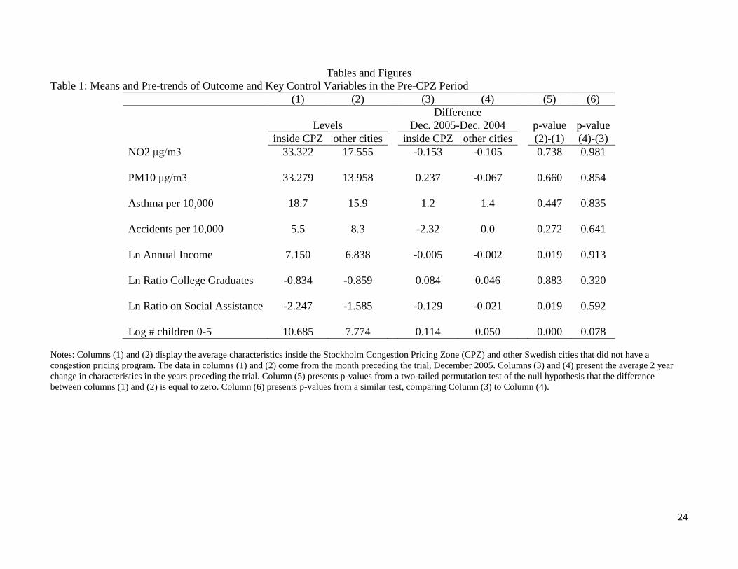
number of monitor observations within each month. The first two rows of Table 1 show the
average levels and growth rates in NO2 and PM10 levels for central Stockholm (“inside CPZ”) and
all other central cities in the 2 years preceding the CPZ trial.5 The levels of 33.32 and 33.28
5 For current EPA standards see: https://www3.epa.gov/region1/airquality/pm-aq-standards.html and https://www.epa.gov/no2-pollution/fact-sheets-and-additional-information-regarding-2010-revision-primary-national. Note that for NO2, one part per billion is equal to 1.25 micrograms per cubic meter.
9
micrograms per cubic meter for these two pollutants respectively, can be compared to current EPA
standards for annual average levels of 66.25 micrograms per cubic meter for NO2 and 50
micrograms per cubic meter for PM10. Hence Table 1 shows that the levels of pollution in
Stockholm were below current U.S. EPA standards for these pollutants even prior to the
implementation of congestion pricing. Our results should therefore be interpreted as illustrating
the health benefits of reducing pollution levels below already relatively low levels of ambient air
pollution.
Column (5) of Table 1 presents p-values from a test of the null hypothesis that the levels
are the same inside Stockholm and in other central cities. Column (6) shows p-values from a test
of the null hypothesis that the pre-trends in these pollutants are the same. These p-values are based
on permutation tests (Fisher, 1935; Good, 2005; Dinardo and Lee, 2011). These tests are likely to
yield more reliable p-values for differences between treatments and controls with small samples
(such as our 103 municipalities). The permutation-based test assumes exchangeability of
treatments and controls under the null. In order to conduct the test, we assign treatment status to
different Swedish cities and then re-calculate the differences in mean levels and in pre-trends
between the index city and all other Swedish cities. The p-value corresponds to the percentile of
the distribution where the observed difference falls, relative to the other permutations. For
example, if none of the permutation differences exceeded the actual difference, then the p-value
would be 0. In this group of 103 cities, if for 76 permutations the difference was greater than the
difference between Stockholm and all other cities, then the p-value would be 0.738 (as it is in the
first row of Column 5 of Table 1). The results in the first two rows of columns (5) and (6) suggest
there are no significant differences in pollution pre-trends in the 2 years preceding the CPZ trial.
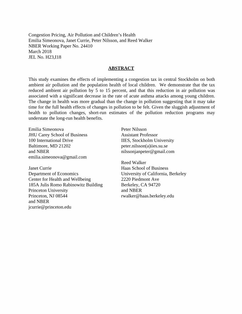
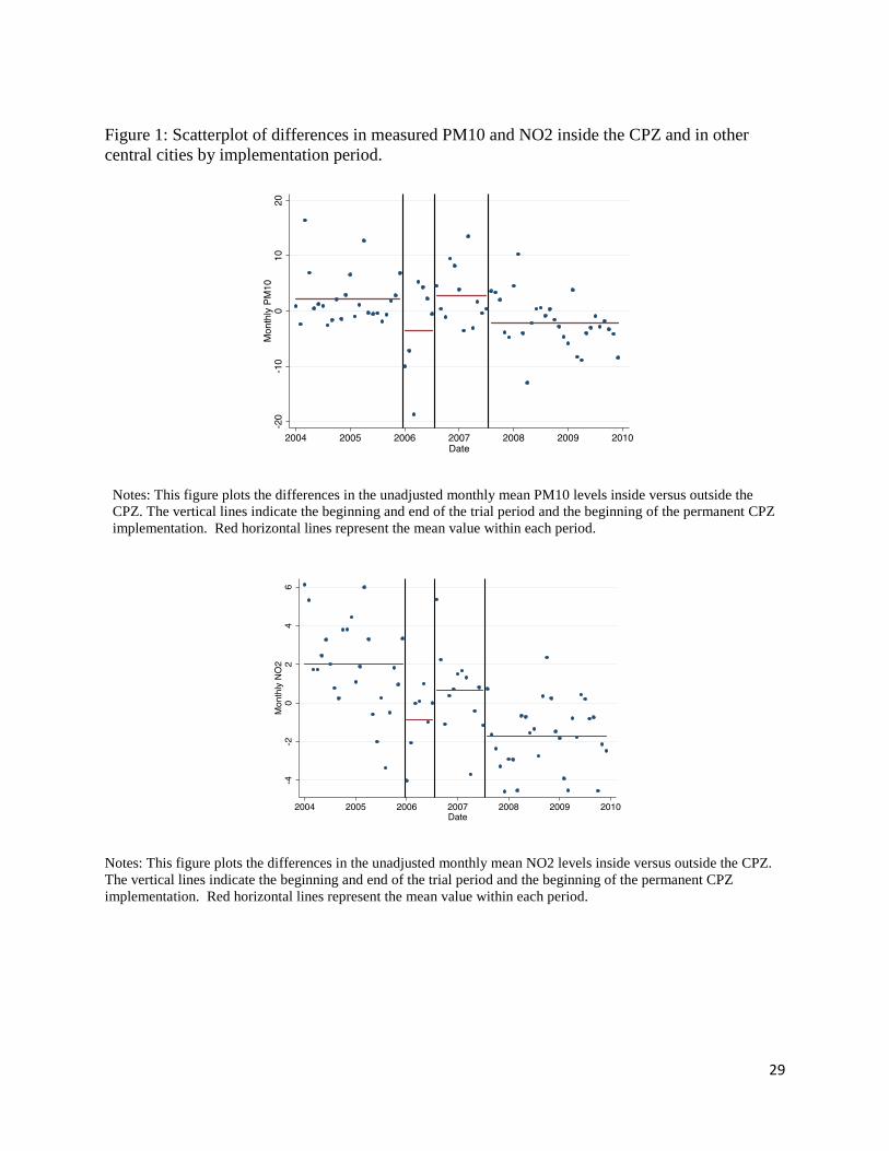
Figure 1 shows the differences in PM10 and NO2 between the Stockholm CPZ and other
Swedish central cities in each month of the sample. The vertical lines indicate the “pre,” “trial,”
10
“in between,” and “permanent CPZ” periods. The points show the differences in monthly averages
representing data from the entire set of available monitors, and the horizontal lines show the mean
differences in pollution levels within each time period. In total, we have 72 months of data. For
both PM10 and NO2, one sees a relative reduction in pollution during the trial period, a rebound
in the “in-between” period, and a larger relative reduction in Stockholm compared to other central
cities once the CPZ is made permanent.
Health data were collected from the inpatient (Swedish National Patient Register
(Socialstyrelsen, 2009)) and outpatient registries. The inpatient register contains administrative
information such as date of admission, number of days in hospital care, as well as discharge
diagnoses classified according to the 9th and 10th versions of International Classification of
Diseases (ICD). The National Patient Register records all hospital admission that included an
overnight hospital stay whether or not it originated in the Emergency Room.
The outpatient register contains information on all outpatient visits to primary care
providers and specialists including visits to Emergency Rooms that did not result in inpatient
admissions. The date of the visit and the primary ICD 9 (or ICD10) code that was the main reason
for the visit are also provided. Importantly, the register records whether the visit was planned (such
as a routine yearly physical check-up) or urgent. Urgent outpatient visits are same-day visits that
are initiated at the request of the patient and usually concern an acute health problem that would
be treated as an emergency on an outpatient basis.
To construct an acute asthma rate, we add the number of overnight hospital visits and the
unscheduled outpatient visits which record asthma as the primary reason for the visit. We then
calculate the cumulative number of acute asthma episodes for each calendar month among children
aged 0 to 5 in the municipality and divide by the total number of resident children.
11
Table 1 shows that at 18.7 cases per 10,000 children 0 to 5, the asthma rate was higher in
central Stockholm than in other central cities, and the rate was rising during the pre-period in both
Stockholm and in other central cities. The p-values shown in column (6) show that there were,
however, no significant differences in these trends between Stockholm and other central cities.
For comparison, we also examine visits for injuries (accidents) among children 0 to 5.
Injuries are one of the most common reasons for children to seek medical attention, and they should
not be mechanically related to air pollution and/or asthma though of course injuries from car
accidents could be reduced by the absence of cars from the inner city. The baseline incidence of
accidents was lower in Stockholm than in other central cities. However, once again the p-values
in Table 1 show that there was no difference in pre-trends.
Table 1 also shows pre-trends in several measures of the socioeconomic status of parents
as well as a measure of city size. While the Stockholm CPZ is much larger, has higher income,
more college graduates, and fewer people on social assistance than other Swedish central cities,
differences in the pre-trends in these variables are not generally statistically significant.
In all of our regression results, we control for weather conditions that may affect the extent
of ambient air pollution independent of the congestion pricing policy. We use data from the
Swedish Meteorological Institute that come from weather stations in each municipality. The
weather data is linked to each city using the inverse distance weighted average of all weather
monitors within 100km of the municipal center. Daily data on rain (mm), rain squared, mean
temperature, temperature squared, maximum temperature, minimum temperature, average wind
speed, and maximum wind speed is calculated for each weather monitor and then aggregated to
the municipality by month level.
12
IV. Methods
We first investigate the extent to which both the Stockholm congestion trial and the
eventual full implementation of the congestion fee affected ambient air pollution. Formally, we
estimate the following equation which allows the effects of the trial, the “in-between” period, and
the period after the charges were made permanent to be distinguished:
(1) Pollit = β1CPZi*Trialt + β2CPZi*InBetweent + β3CPZi*Permanentt + Zitγ + υi + Wit + εit
where Trial, InBetween, and Permanent are dummy variables equal to one during the relevant
periods. Pollution at monitor i in month t (𝑃𝑃𝑃𝑃𝑃𝑃𝑃𝑃𝑖𝑖𝑖𝑖) is regressed on a set of interactions, where, for
example, CPZi*Trialt is an indicator equal to one if the period is one in which the congestion trial
is in place and the pollution monitor is in the CPZ zone. Equation (1) also includes monitor fixed
effects υi, weather controls, Wit, year by month fixed effects, and monitor-specific time trends, Zit.
The coefficients 𝛽𝛽1 and 𝛽𝛽3 measure the shorter and longer-run effects of implementing
congestion pricing, while 𝛽𝛽2 measures whether the dependent variable returned to “baseline”
during the “in-between” period. Monitor fixed effects ensure that the identifying variation comes
from within-monitor changes in air pollution in periods with congestion pricing versus periods
without. The main identifying assumption is that even if the levels of pollution were different
between Stockholm and other municipalities, the trends did not differ systematically for reasons
other than the implementation of congestion pricing. This assumption is the motivation for testing
for differing pre-trends in pollution, as was discussed above. Since the issue of differential trends
is potentially important, we also include both region-specific time trends and interactions between
municipality and weather controls. These latter interactions allow for the fact that the same
weather patterns could have different impacts on pollution levels in different cities.
13
We examine asthma rates using models that take much the same form as equation (1)
except that they use measures of asthma rates constructed at the municipality, month, and year
level as the dependent variable. Now Zjt is a vector of time-varying controls including the average
family income in municipality j in month t, the proportion of the population on social support, and
the proportion with a college degree, as well as a vector of year by month fixed effects. Once
again we include controls for monthly weather conditions. Instead of fixed effects for pollution
monitors, we include fixed effects for each municipality, so that our models are identified using
within-municipality variation in asthma rates. The identifying assumption is that there would have
been parallel trends in asthma in the absence of the CPZ. We provided some evidence in support
of this assumption by examining pre-trends in Table 1.
We also use all of the data, aside from that collected in central Stockholm while congestion
pricing was in effect, in order to model asthma rates in the rest of the sample, and then ask whether
the predicted asthma rates in central Stockholm from this model changed with the implementation
of the CPZ. This test assesses the degree to which the underlying demographics and other
observables changed in Stockholm in a way that would predict changes in asthma rates during the
CPZ period. Finally, as a comparison we also examine the “effects” of the CPZ on childhood
injuries.
All regressions with asthma or injury as a dependent variable are estimated by weighted
least squares using the number of children aged 0 to 5 in the municipality as weights.
V. Results
a) Congestion Pricing and Pollution Levels
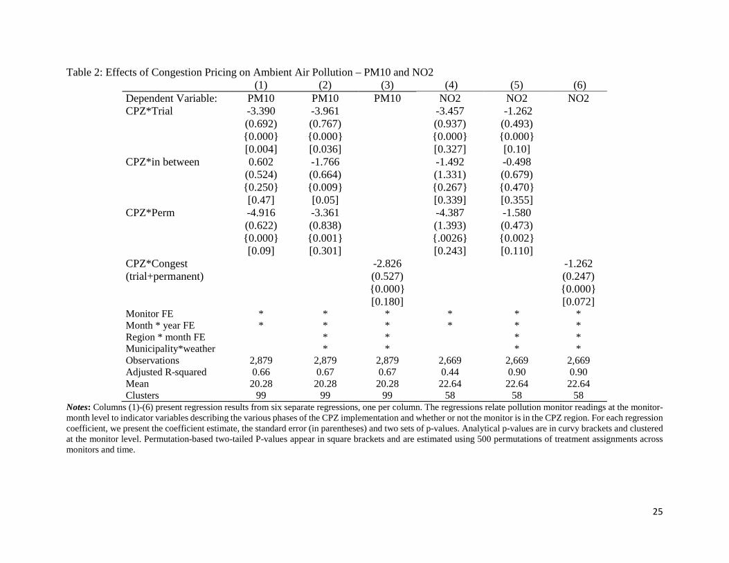
Table 2 presents estimates for the effects of the CPZ on levels of PM10 and NO2. We show
the usual analytical standard errors in parentheses, and we present two sets of p-values: p-values
14
that correspond to the analytical standard errors are shown in curvy brackets, and permutation-
based p-values which are shown in square brackets. The permutation-based values are based on
500 simulations in which the type of CPZ “treatment” (trial, in between, or permanent) is randomly
assigned across municipalities semi-annually, so that the permuted cells represent each
municipality in each 6-month period during the observation window (see e.g., Cesarini et al
(2016)). For each outcome and each permuted sample we estimate equation (1). We then examine
the fraction of the times that the coefficient estimate exceeds the estimated value when the CPZ is
correctly assigned to Stockholm.
The estimates and analytic p-values in columns (1) and (4) of Table 2 are consistent with
Figure 1 in that they suggest that both PM10 and NO2 declined during the trial, rebounded during
the in-between period, and settled at a lower level similar to that seen during the trial when the
CPZ became permanent. Specifications including controls for location-specific weather and
region-specific seasonality confirm these findings. The permutation based p-values are more
conservative but also support this story. While we cannot completely rule out the hypothesis that
PM10 and NO2 levels went back to the pre-trial levels during the in-between period, there is
evidence that they remained at somewhat lower levels. This inference is consistent with the
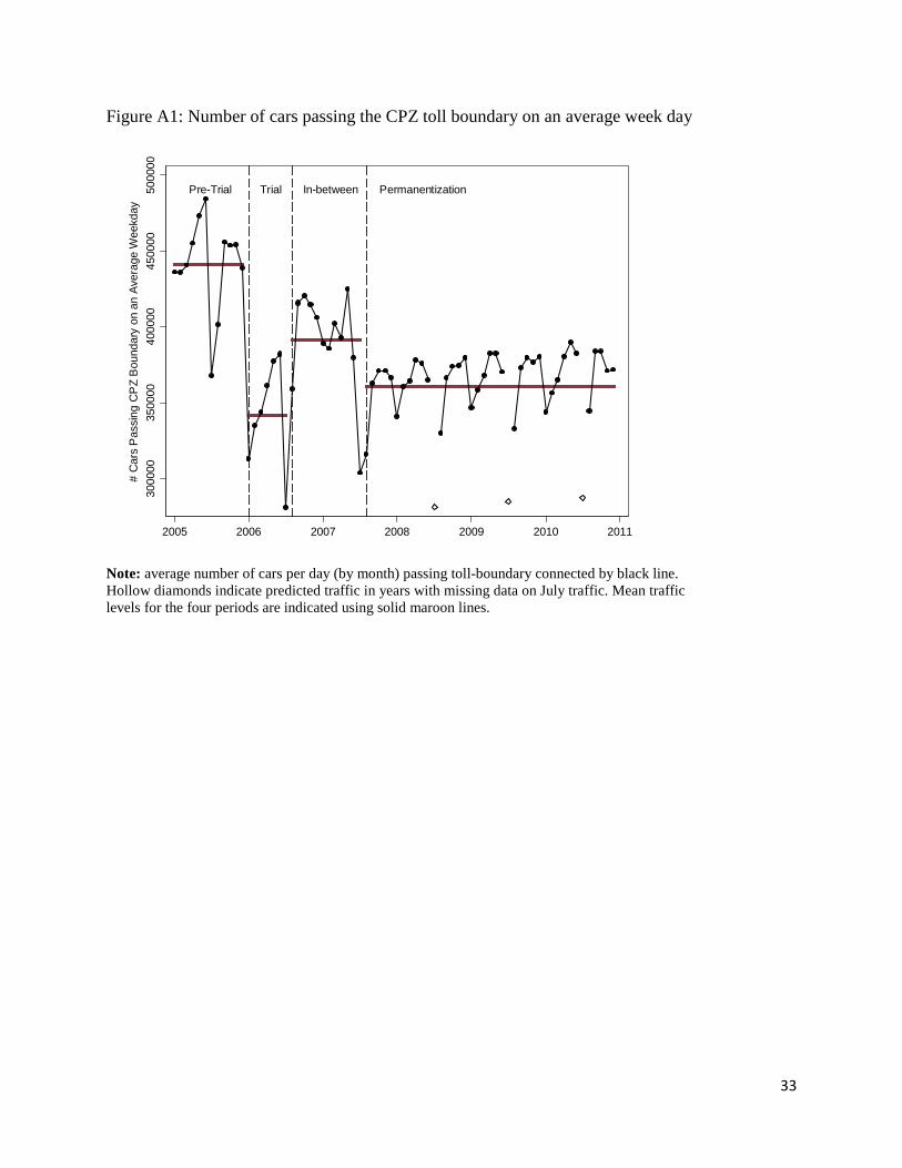
available data on traffic flows, which show a persistant reduction of 10 percent relative to baseline
levels during the in-between period. (See Appendix Figure A1).
The 3.36 unit decline in PM10 and the 1.58 unit decline in NO2 after the CPZ was made
permanent correspond to a 10% and a 5% reduction in these two pollutants relative to the mean
levels of pre-CPZ pollution in Stockholm shown in Table 1. The estimates in column (3) show
that if one did not allow for the lack of a full “rebound” effect during the in-between period, one
would get a slightly lower estimate of the impact of congestion pricing on pollution.
15
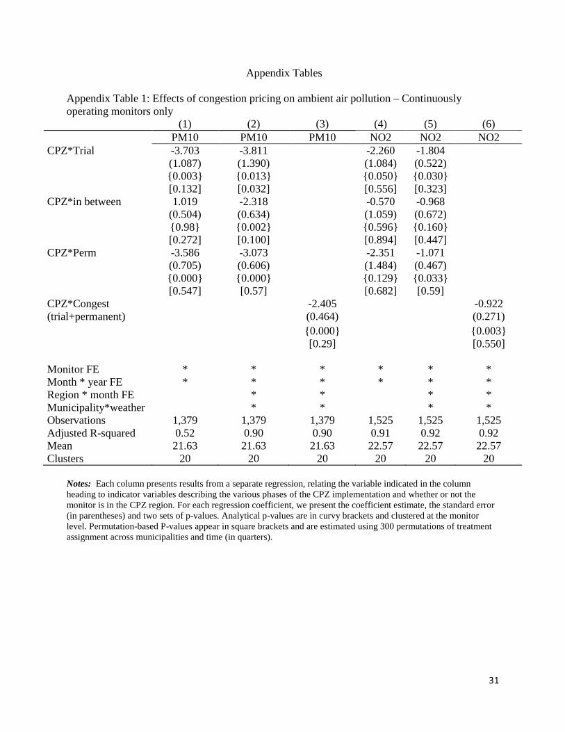
Appendix Table 1 shows an alternative specification which uses only data from monitors
that were continuously operating. Using a fixed set of monitors alleviates any concerns about
selection due to monitor entry and exit but on the other hand, there are many fewer continuously
operating monitors. The point estimates in Appendix Table 1 are remarkably similar to those
discussed above, and the analytic p-values suggest significant negative effects on pollution in both
the trial and the permanent CPZ periods. The permutation based tests confirm a negative effect of
congestion pricing on PM10, but do not allow rejections of the null during the permanent
implementation period. Overall, Appendix Table 1 re-affirms that the Stockholm CPZ was
associated with significant pollution reductions.
b) Congestion Pricing and Asthma
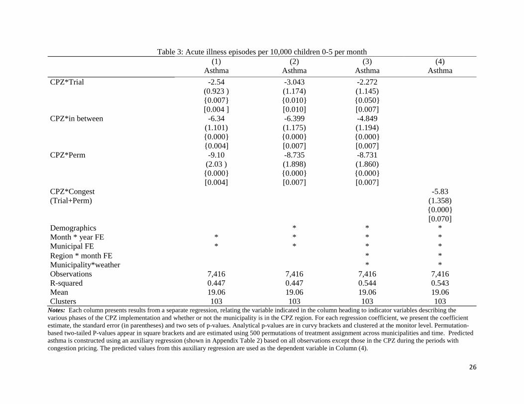
The estimated effects of the CPZ on asthma rates in children aged 0-5 are shown in columns
(1) through (4) of Table 3. Column (1) shows the basic specification controlling for month-specific
and municipality-specific fixed effects. In column (2) we add controls for average income, the
fraction of individuals on social assistance, and the fraction of mothers with completed college
education in the municipality. The coefficients of interest are not affected by these additions. A
comparison of columns (1) and (3) shows that the estimates are also quite robust to the inclusion
of interactions of month fixed effects with region (in order to allow for different regional seasonal
effects) and interactions of weather and municipality (in order to allow weather conditions to have
differential effects in different cities).
However, unlike the pollution estimates which show a reduction in pollution, followed by
a rebound, and then a permanent reduction, column (3) shows that the congestion pricing trial was
associated with a continuous decline in asthma cases in Stockholm relative to other central cities
from the trial period onwards. There was a reduction of 2.3 asthma visits per 10,000 children (on
16
a baseline of 18.7 visits per 10,000) during the trial. The “in-between” period saw a reduction of
4.8 cases per 10,000, while the permanent CPZ reduced asthma visits by about 8.7 per 10,000.
These estimates suggest that the trial brought an immediate reduction in asthma rates, but that the
permanent CPZ had a much larger effect, reducing urgent visits and hospitalizations for asthma by
almost half among children 0 to 5. In these models the analytical and permutation-based p-values
are very close to each other, and both suggest that the estimated effects are strongly statistically
significant. In the last column we group the trial and the permanentization period under one
category of congestion pricing and consider the in-between period as a non-congestion pricing
period. Column (4) indicates that overall, congestion pricing was associated with a reduction of
5.83 asthma visits per 10,000 children.
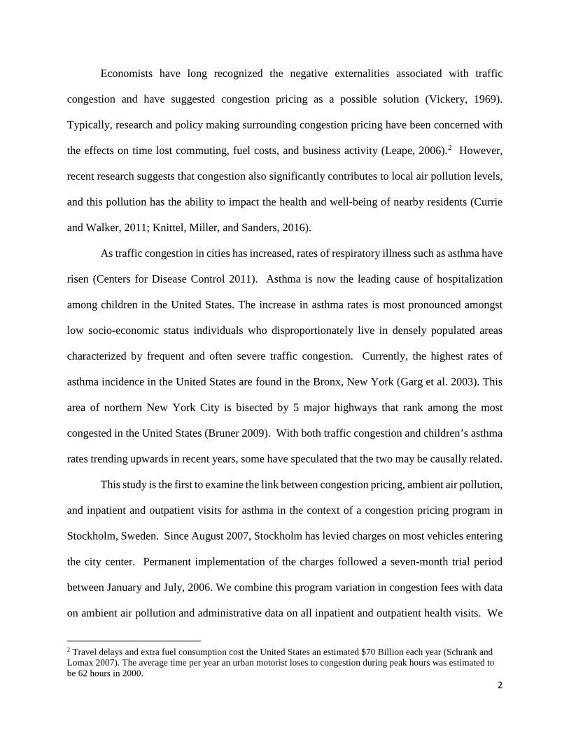
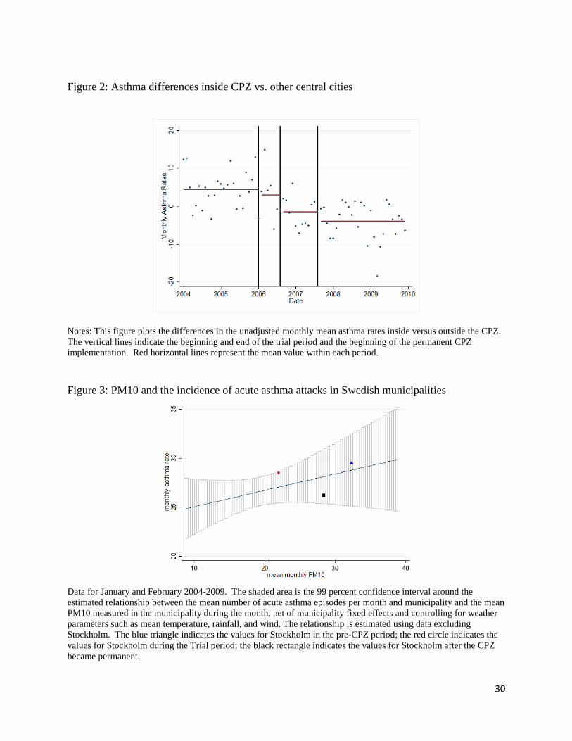
Figure 2 follows a format similar to Figure 1 and shows the difference in asthma rates by
calendar month in Stockholm compared to other central cities before and after the adoption of
congestion pricing. This figure shows an initial decline in asthma in Stockholm relative to the
other central cities during the trial period. However, instead of rebounding, relative asthma rates
in Stockholm vs. other cities continued to decline in the “in between” period, and fell to their
lowest levels after the CPZ became permanent.
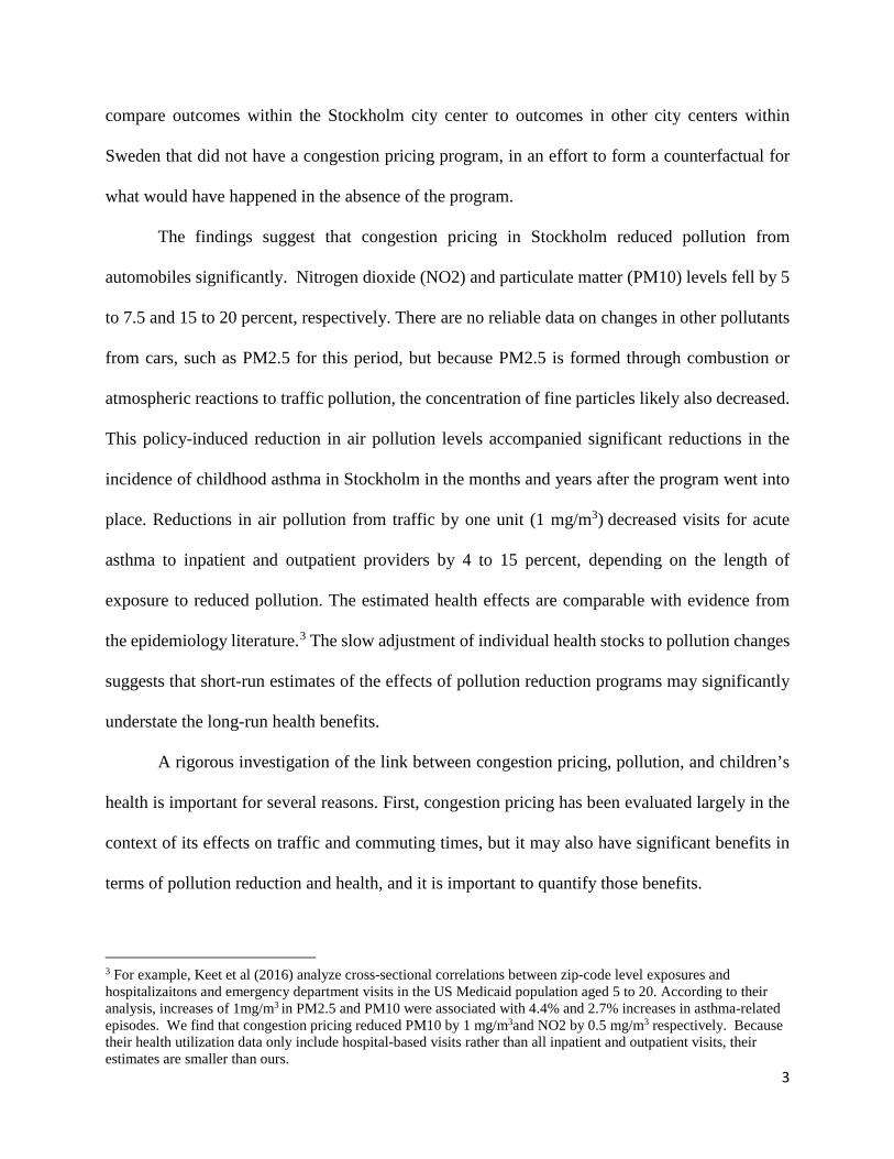
Figure 3 provides some insight into whether the changes in asthma rates accompanying
congestion pricing are “reasonable” given the overall relationships observed between pollution
and asthma in Sweden. The figure is based on data for January and February 2004 to 2009 for
each month and municipality except Stockholm. We use January and February because asthma is
highly seasonal, and these are peak months. The line shows the relationship between the monthly
asthma rate and the mean monthly PM10 level conditional on municipal fixed effects, mean
temperature, mean rainfall, and average wind speed. The shaded area is the 99 percent confidence
interval. The indicated points show values for Stockholm. The blue triangle indicates Stockholm
17
in the pre-CPZ period; the red circle indicates Stockholm during the trial period; the black
rectangle indicates the values for Stockholm after the CPZ became permanent. All Stockholm-
specific data points are within the 99 percent confidence interval of the estimated association
between asthma and mean PM10. The figure demonstrates that the fall in asthma rates in
Stockholm is within the range that one would expect given the relationship between pollution and
asthma rates in the rest of Sweden.
c) Robustness
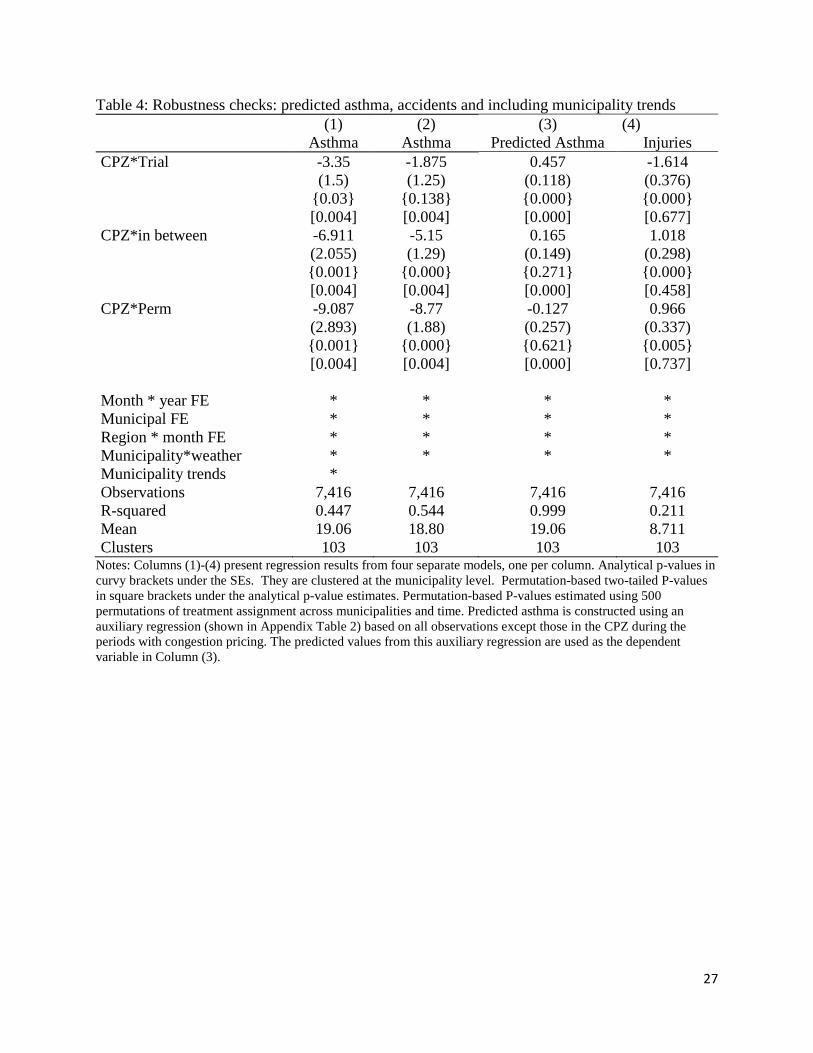
Table 4 presents results from several robustness checks of our main results. The specification
in column (1) includes municipality-specific linear trends. Including these trends should absorb
any unobserved municipality-specific changes in the asthma prevalence that happen during the
observation period. The coefficients of interest do not change significantly. In column (2) we
assign the first municipality in which children are observed as their permanent municipality of
residence. For example, if a child was born in Stockholm, but moved outside the city after a couple
of years, we would now include this child as part of the Stockholm sample for all years included
in the observation window. Similarly, if a child moved into Stockholm, but was first observed as
residing in another city, we would now assign the original city as that child’s residence throughout
the observation window. Constructing the analysis sample in this fashion may address concerns
about children differentially moving in or out of Stockholm based on their health status. On the
other hand, we are introducing noise in the treatment variable, which could bias our estimates
downward. However, the estimates shown in Column (3) appear quite robust to specifying the
analysis sample in this way.
Column (3) of Table 4 shows estimates from a model using predicted asthma rates as the
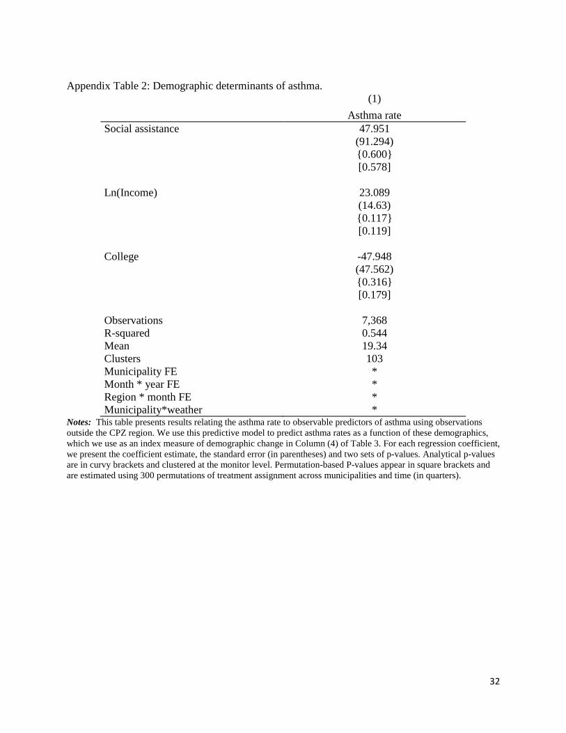
dependent variable. The prediction equation itself is shown in Appendix Table 2. Because we saw
18
in Table 1 that rates of social assistance use and income levels in Stockholm are different than in
other central cities, it is reassuring that neither of these variables are predictive of asthma rates in
our baseline model which includes municipality fixed effects, interactions between month and
year, interactions between region and month, and interactions between municipality and weather
are included in the model. However, with an R-squared of .544, we do a reasonably good job
explaining variation in asthma rates.
The estimated models using predicted asthma as the dependent variable suggest that
changes in the congestion pricing program led to changes in observable characteristics that are
predictive of small but significant increases in the asthma rate in the short run, followed by an
equally small decrease in asthma rates when the CPZ became permanent. While there may be other
changes in unobservables that are correlated with both asthma and the congestion program, the
evidence presented here suggests that changes in observable characteristics cannot explain the
baseline asthma results.
Column (4) of Table 4 presents estimates where the dependent variable is visits due to
injuries. This model takes the same form as the model of asthma. The analytical standard errors
suggest small but significant effects: An initial decline during the trial followed by a rebounding
during the in-between and CPZ permanent periods so that by the end of the period there was no
overall change. The permutation-based p-values are more conservative and suggest that none of
the estimated effects on injuries are statistically significant. This “placebo” like test suggests then
that the CPZ implementation had limited or no effect on non-respiratory health outcomes in this
age group.
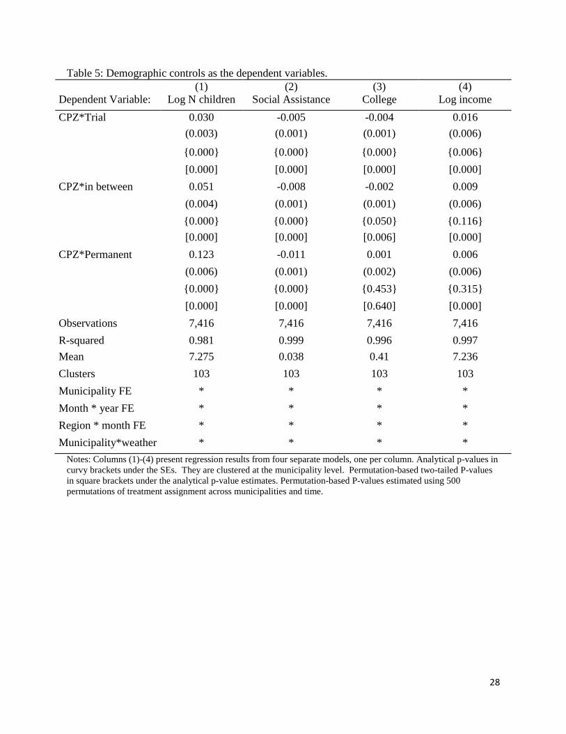
Table 5 presents models in the same form but using demographic characteristics as the
dependent variables. The purpose of these regressions is to assess the extent to which the
reductions in asthma rates that accompanied congestion pricing could have been due to changes in
19
demographic characteristics rather than with congestion pricing per se. Table 5 shows that there
were significant changes. More children came to Stockholm than to other central cities. However,
this tended to reduce the number of children on social assistance, reduce the fraction whose
mothers had a college education, and increase relative income levels. As we show in Appendix
Table 2, demographic characteristics are at best weakly correlated with asthma rates in Sweden.
Still, for the two variables that are close to statistically significantly predictive of asthma – college
education and income - the population changes we document in Stockholm would have been
expected to increase, rather than to decrease, asthma rates. Hence, it appears that congestion
pricing reduced asthma rates in the face of demographic changes that might have been expected to
increase them.
VI. Discussion and Conclusions
This paper estimates the impact of a congestion pricing program in a large urban center on ambient
pollution and children’s health as proxied by childhood asthma rates. Our findings indicate that
the congestion tax in central Stockholm reduced ambient pollution levels. The two pollutants we
can measure best, PM10 and NO2, declined between 5 and 20 percent. This decline suggests that
other pollutants from traffic are also likely to have fallen. Declines in relative ambient pollution
levels in Stockholm compared to other central cities show a step-wise pattern, first falling during
the trial period, then rebounding somewhat during the period in between the trial and permanent
adoption, and then showing a sustained decline following permanent adoption of congestion
pricing.
This policy-induced change in pollution from traffic is associated with a significant
reduction in the rate of acute asthma attacks among children 0 to 5 years of age in the years after
the program. Although congestion pricing had an immediate impact on asthma, the impact grew
20
over time and asthma rates actually continued to decline during what proved to be a temporary
hiatus in congestion pricing before the permanent adoption of the policy. Our findings therefore
suggest that congestion charges in large cities can have significant positive effects on health in the
short-term, but even larger effects in the longer term as the stock of health evolves to a new lower-
pollution equilibrium level. This finding is consistent with our understanding of health as a stock
that often changes relatively slowly over time, as suggested by the medical literature.
Our estimates are among the first to demonstrate that congestion pricing as implemented
in Stockholm resulted in a significant decrease in ambient air pollution due to automobiles, and
significant impacts in children’s respiratory health. These improvements in health occurred even
though initial pollution levels were well below the current U.S. EPA standards, suggesting that
reductions in pollution from traffic can have large positive effects on children’s respiratory health
in many settings.
21
References Avol, Edward, James Gauderman, Sylvia Tan, Stephanie London and John Peters (2001) “Respiratory Effects of Relocating to Areas of Differing Air Pollution Levels” American Journal of Respiratory and Critical Care Medicine, Vol 164, No 11 Bauernschuster, Stefan, Timo Hener and Helmut Rainer (2015). “When Labor Disputes Bring Cities to a Standstill: The Impact of Public Transit Strikes on Traffic, Accidents, Air Pollution and Health,” Ifo Institute Working paper. Bruner, Jon. 2009. “America’s Worst Intersections.” Forbes Cesarini, David, Erik Lindqvist, Robert Ostling and Björn Wallace (2016) “Wealth, Health, and Child Development: Evidence from Administrative Data on Swedish Lottery Players”, forthcoming, Quarterly Journal of Economics. Chen, Yuyu, Avraham Ebenstein, Michael Greenstone, and Hongbin Li (2013). ”Evidence on the Impact of Sustained Exposure to Air Pollution on Life Expectancy from China’s Huai River Policy,” Proceedings of the National Academy of Sciences, v 110 #32, pp 12936–12941. Currie, Janet and Reed Walker (2011) ”Traffic Congestion and Infant Health: Evidence from E-Zpass” American Economic Journal: Applied Economics v3, January, 65-90. Currie, Janet, Joshua Graff Zivin, Jamie Mullins and Matthew Neidell (2014). “What Do We Know about Short and Long-Term Effects of Early Life Exposure to Pollution?” Annual Review of Resource Economics v. 6, October, 217-247. Dietert RR, Etzel RA, Chen D, et al. (2000). Workshop to identify critical windows of exposure for children’s health: immune and respiratory systems work group summary. Environmental Health Perspectives, v108(suppl 3):483– 490. Dinardo, John and David Lee (2011). “Program Evaluation and Research Designs,” in Orley Ashenfelter and David E. Card (eds.) Handbook of Labor Economics, v4A (North Holland: New York, Amsterdam). Fisher, Sir Ronald Aylmer (1935). Design of Experiments (Edinburgh, London: Oliver and Boyd). Fletcher, Jason, Jeremy Green and Matthew Neidell (2010) “Long term effects of childhood asthma on adult health” Journal of Health Economics, Volume 29, Issue 3, May, 377–387. Friedman, Michael S., Kenneth E. Powell, Lori Hutwagner, LeRoy M. Graham, and W. Gerald Teague. 2001. “Impact of Changes in Transportation and Commuting Behaviors During the 1996 Summer Olympic Games in Atlanta on Air Quality and Childhood Asthma.” Journal of the American Medical Association, 285(7): 897–905
22
Garg, Renu, Adam Karpati, Jessica Leighton, Mary Perrin, and Mona Shah. 2003. Asthma Facts. Second ed., New York City Department of Health and Mental Hygiene Gauderman WJ, McConnell R, Gilliland F, et al. (2000). “Association between air pollution and lung function growth in southern California children,” Am J Respir Crit Care Med. v162:1383–1390. Good, Phillip (2005). Permutation, Parametric, and Bootstrap Tests of Hypotheses (Springer, New York). Hoek G, Dockery DW, Pope A, Neas L, Roemer W, Brunekreef B. (1998). “Association between PM10 and decrements in peak expiratory flow rates in children: reanalysis of data from five panel studies,” Eur Respir J. v11:1307–1311. Jans, Jenny, Per Johansson, and J Peter Nilsson (2016), "Economic Status, Air Quality, and Child Health: Evidence from Inversion Episodes" manuscript April 2016, Stockholm university Kim, J.J. et al. (2004) “Ambient Air Pollution: Health Hazards to Children” American Academy of Pediatrics Policy Statement; Pediatrics v114, 1699. Knittel, Miller, and Sanders (2016) “Caution, Drivers! Children Present: Traffic, Pollution, and Infant Health” The Review of Economics and Statistics, May 2016, Vol. 98, No. 2, Pages: 350-366 Leape, Jonathan. 2006. "The London Congestion Charge." Journal of Economic Perspectives, 20(4): 157-176. Lipsett M, Hurley S, Ostro B (1997). “Air pollution and emergency room visits for asthma in Santa Clara County, California,” Environmental Health Perspectives v105:216 –222. McConnell, Rob, Kiros Berhane, Ling Yao, Michael Jerrett, Fred Lurmann, Frank Gilliland, Nino Kunzli, Jim Gauderman, Ed Avol, Duncan Thomas, and John Peters (2006) ”Traffic, Susceptibility, and Childhood Asthma,” Environmental Health Perspectives, Volume 114 #5, May, 766-772. Moorman, Jeanne, Cara Person, Hatice Zahran (2013). “Asthma Attacks Among Persons with Current Asthma – United States, 2001-2010,” Morbidity and Mortality Weekly Report, Nov. 22, v62 #3: 93-98. Neidell, Matthew (2004) “Air pollution, health, and socio-economic status: the effect of outdoor air quality on childhood asthma,” Journal of Health Economics, Volume 23, Issue 6, November, 1209–1236 Enrico Moretti and Matthew Neidell (2011) “Pollution, Health, and Avoidance Behavior Evidence from the Ports of Los Angeles” Journal of Human Resources, vol 46, no 1, pp 154-175 Pinkerton KE, Joad JP (2000). “The mammalian respiratory system and critical windows of exposure for children’s health,” Environmental Health Perspectives v108(suppl 3):457– 462.
23
Pope, C. Arden, R.T. Burnett, M.J. Thun, E.E. Calle, D. Krewski, K. Ito, G.D. Thurston (2002). “Lung Cancer, Cardiopulmonary Mortality, and Long-Term Exposure to Fine Particulate Air Pollution,” JAMA 287 #9, 1132-1141. Schlenker, Wolfram and Reed Walker (2015) “Airports, Air Pollution and Contemporaneous Health” Review of Economic Studies, October, 2015 Shima M, Adachi M (2000). “Effect of outdoor and indoor nitrogen dioxide on respiratory symptoms in schoolchildren,” Int J Epidemiol. v29: 862– 870. David Schrank and Tim Lomax (2007) “The 2007 Urban Mobility Report” Texas Transportation Institute, Texas A&M University, September 2007 (accessible at http://www.ncga.state.nc.us/documentsites/committees/21stcenturytransportation/prioritization-best%20practices-efficiency/presentations/mobility_report_2007_wappx.pdf) U.S. Environmental Protection Agency NAAQS table (https://www.epa.gov/criteria-air-pollutants/naaqs-table) U.S. National Asthma Education and Prevention Program (2007). Third Expert Panel on the Diagnosis and Management of Asthma. Bethesda (MD): National Heart, Lung, and Blood Institute (US); Aug. Yu O, Sheppard L, Lumley T, Koenig JQ, Shapiro GG (2000). “Effects of ambient air pollution on symptoms of asthma in Seattle-area children enrolled in the CAMP study,” Environmental Health Perspectives v108: 1209 –1214.
24
Tables and Figures Table 1: Means and Pre-trends of Outcome and Key Control Variables in the Pre-CPZ Period
(1) (2) (3) (4) (5) (6)
Levels Difference
Dec. 2005-Dec. 2004 p-value p-value inside CPZ other cities inside CPZ other cities (2)-(1) (4)-(3)
NO2 μg/m3 33.322 17.555 -0.153 -0.105 0.738 0.981 PM10 μg/m3 33.279 13.958 0.237 -0.067 0.660 0.854 Asthma per 10,000 18.7 15.9 1.2 1.4 0.447 0.835 Accidents per 10,000 5.5 8.3 -2.32 0.0 0.272 0.641 Ln Annual Income 7.150 6.838 -0.005 -0.002 0.019 0.913 Ln Ratio College Graduates -0.834 -0.859 0.084 0.046 0.883 0.320 Ln Ratio on Social Assistance -2.247 -1.585 -0.129 -0.021 0.019 0.592 Log # children 0-5 10.685 7.774 0.114 0.050 0.000 0.078
Notes: Columns (1) and (2) display the average characteristics inside the Stockholm Congestion Pricing Zone (CPZ) and other Swedish cities that did not have a congestion pricing program. The data in columns (1) and (2) come from the month preceding the trial, December 2005. Columns (3) and (4) present the average 2 year change in characteristics in the years preceding the trial. Column (5) presents p-values from a two-tailed permutation test of the null hypothesis that the difference between columns (1) and (2) is equal to zero. Column (6) presents p-values from a similar test, comparing Column (3) to Column (4).
25
Table 2: Effects of Congestion Pricing on Ambient Air Pollution – PM10 and NO2 (1) (2) (3) (4) (5) (6) Dependent Variable: PM10 PM10 PM10 NO2 NO2 NO2 CPZ*Trial -3.390 -3.961 -3.457 -1.262 (0.692) (0.767) (0.937) (0.493) {0.000} {0.000} {0.000} {0.000} [0.004] [0.036] [0.327] [0.10] CPZ*in between 0.602 -1.766 -1.492 -0.498 (0.524) (0.664) (1.331) (0.679) {0.250} {0.009} {0.267} {0.470} [0.47] [0.05] [0.339] [0.355] CPZ*Perm -4.916 -3.361 -4.387 -1.580 (0.622) (0.838) (1.393) (0.473) {0.000} {0.001} {.0026} {0.002} [0.09] [0.301] [0.243] [0.110] CPZ*Congest -2.826 -1.262 (trial+permanent) (0.527) (0.247) {0.000} {0.000} [0.180] [0.072] Monitor FE * * * * * * Month * year FE * * * * * * Region * month FE * * * * Municipality*weather * * * * Observations 2,879 2,879 2,879 2,669 2,669 2,669 Adjusted R-squared 0.66 0.67 0.67 0.44 0.90 0.90 Mean 20.28 20.28 20.28 22.64 22.64 22.64 Clusters 99 99 99 58 58 58
Notes: Columns (1)-(6) present regression results from six separate regressions, one per column. The regressions relate pollution monitor readings at the monitor-month level to indicator variables describing the various phases of the CPZ implementation and whether or not the monitor is in the CPZ region. For each regression coefficient, we present the coefficient estimate, the standard error (in parentheses) and two sets of p-values. Analytical p-values are in curvy brackets and clustered at the monitor level. Permutation-based two-tailed P-values appear in square brackets and are estimated using 500 permutations of treatment assignments across monitors and time.
26
Table 3: Acute illness episodes per 10,000 children 0-5 per month (1) (2) (3) (4) Asthma Asthma Asthma Asthma CPZ*Trial -2.54 -3.043 -2.272 (0.923 ) (1.174) (1.145) {0.007} {0.010} {0.050} [0.004 ] [0.010] [0.007] CPZ*in between -6.34 -6.399 -4.849 (1.101) (1.175) (1.194) {0.000} {0.000} {0.000} {0.004] [0.007] [0.007] CPZ*Perm -9.10 -8.735 -8.731 (2.03 ) (1.898) (1.860) {0.000} {0.000} {0.000} [0.004] [0.007] [0.007] CPZ*Congest -5.83 (Trial+Perm) (1.358) {0.000} [0.070] Demographics * * * Month * year FE * * * * Municipal FE * * * * Region * month FE * * Municipality*weather * * Observations 7,416 7,416 7,416 7,416 R-squared 0.447 0.447 0.544 0.543 Mean 19.06 19.06 19.06 19.06 Clusters 103 103 103 103
Notes: Each column presents results from a separate regression, relating the variable indicated in the column heading to indicator variables describing the various phases of the CPZ implementation and whether or not the municipality is in the CPZ region. For each regression coefficient, we present the coefficient estimate, the standard error (in parentheses) and two sets of p-values. Analytical p-values are in curvy brackets and clustered at the monitor level. Permutation-based two-tailed P-values appear in square brackets and are estimated using 500 permutations of treatment assignment across municipalities and time. Predicted asthma is constructed using an auxiliary regression (shown in Appendix Table 2) based on all observations except those in the CPZ during the periods with congestion pricing. The predicted values from this auxiliary regression are used as the dependent variable in Column (4).
27
Table 4: Robustness checks: predicted asthma, accidents and including municipality trends (1) (2) (3) (4) Asthma Asthma Predicted Asthma Injuries CPZ*Trial -3.35 -1.875 0.457 -1.614 (1.5) (1.25) (0.118) (0.376) {0.03} {0.138} {0.000} {0.000} [0.004] [0.004] [0.000] [0.677] CPZ*in between -6.911 -5.15 0.165 1.018 (2.055) (1.29) (0.149) (0.298) {0.001} {0.000} {0.271} {0.000} [0.004] [0.004] [0.000] [0.458] CPZ*Perm -9.087 -8.77 -0.127 0.966 (2.893) (1.88) (0.257) (0.337) {0.001} {0.000} {0.621} {0.005} [0.004] [0.004] [0.000] [0.737] Month * year FE * * * * Municipal FE * * * * Region * month FE * * * * Municipality*weather * * * * Municipality trends * Observations 7,416 7,416 7,416 7,416 R-squared 0.447 0.544 0.999 0.211 Mean 19.06 18.80 19.06 8.711 Clusters 103 103 103 103
Notes: Columns (1)-(4) present regression results from four separate models, one per column. Analytical p-values in curvy brackets under the SEs. They are clustered at the municipality level. Permutation-based two-tailed P-values in square brackets under the analytical p-value estimates. Permutation-based P-values estimated using 500 permutations of treatment assignment across municipalities and time. Predicted asthma is constructed using an auxiliary regression (shown in Appendix Table 2) based on all observations except those in the CPZ during the periods with congestion pricing. The predicted values from this auxiliary regression are used as the dependent variable in Column (3).
28
Table 5: Demographic controls as the dependent variables. (1) (2) (3) (4) Dependent Variable: Log N children Social Assistance College Log income CPZ*Trial 0.030 -0.005 -0.004 0.016 (0.003) (0.001) (0.001) (0.006)
{0.000} {0.000} {0.000} {0.006} [0.000] [0.000] [0.000] [0.000] CPZ*in between 0.051 -0.008 -0.002 0.009 (0.004) (0.001) (0.001) (0.006) {0.000} {0.000} {0.050} {0.116} [0.000] [0.000] [0.006] [0.000] CPZ*Permanent 0.123 -0.011 0.001 0.006 (0.006) (0.001) (0.002) (0.006) {0.000} {0.000} {0.453} {0.315} [0.000] [0.000] [0.640] [0.000] Observations 7,416 7,416 7,416 7,416 R-squared 0.981 0.999 0.996 0.997 Mean 7.275 0.038 0.41 7.236 Clusters 103 103 103 103 Municipality FE * * * * Month * year FE * * * * Region * month FE * * * * Municipality*weather * * * *
Notes: Columns (1)-(4) present regression results from four separate models, one per column. Analytical p-values in curvy brackets under the SEs. They are clustered at the municipality level. Permutation-based two-tailed P-values in square brackets under the analytical p-value estimates. Permutation-based P-values estimated using 500 permutations of treatment assignment across municipalities and time.
29
Figure 1: Scatterplot of differences in measured PM10 and NO2 inside the CPZ and in other central cities by implementation period.
Notes: This figure plots the differences in the unadjusted monthly mean PM10 levels inside versus outside the CPZ. The vertical lines indicate the beginning and end of the trial period and the beginning of the permanent CPZ implementation. Red horizontal lines represent the mean value within each period.
Notes: This figure plots the differences in the unadjusted monthly mean NO2 levels inside versus outside the CPZ. The vertical lines indicate the beginning and end of the trial period and the beginning of the permanent CPZ implementation. Red horizontal lines represent the mean value within each period.
30
Figure 2: Asthma differences inside CPZ vs. other central cities
Notes: This figure plots the differences in the unadjusted monthly mean asthma rates inside versus outside the CPZ. The vertical lines indicate the beginning and end of the trial period and the beginning of the permanent CPZ implementation. Red horizontal lines represent the mean value within each period. Figure 3: PM10 and the incidence of acute asthma attacks in Swedish municipalities
Data for January and February 2004-2009. The shaded area is the 99 percent confidence interval around the estimated relationship between the mean number of acute asthma episodes per month and municipality and the mean PM10 measured in the municipality during the month, net of municipality fixed effects and controlling for weather parameters such as mean temperature, rainfall, and wind. The relationship is estimated using data excluding Stockholm. The blue triangle indicates the values for Stockholm in the pre-CPZ period; the red circle indicates the values for Stockholm during the Trial period; the black rectangle indicates the values for Stockholm after the CPZ became permanent.
31
Appendix Tables Appendix Table 1: Effects of congestion pricing on ambient air pollution – Continuously operating monitors only
(1) (2) (3) (4) (5) (6) PM10 PM10 PM10 NO2 NO2 NO2 CPZ*Trial -3.703 -3.811 -2.260 -1.804 (1.087) (1.390) (1.084) (0.522) {0.003} {0.013} {0.050} {0.030} [0.132] [0.032] [0.556] [0.323] CPZ*in between 1.019 -2.318 -0.570 -0.968 (0.504) (0.634) (1.059) (0.672) {0.98} {0.002} {0.596} {0.160} [0.272] [0.100] [0.894] [0.447] CPZ*Perm -3.586 -3.073 -2.351 -1.071 (0.705) (0.606) (1.484) (0.467) {0.000} {0.000} {0.129} {0.033} [0.547] [0.57] [0.682] [0.59] CPZ*Congest -2.405 -0.922 (trial+permanent) (0.464) (0.271) {0.000} {0.003} [0.29] [0.550] Monitor FE * * * * * * Month * year FE * * * * * * Region * month FE * * * * Municipality*weather * * * * Observations 1,379 1,379 1,379 1,525 1,525 1,525 Adjusted R-squared 0.52 0.90 0.90 0.91 0.92 0.92 Mean 21.63 21.63 21.63 22.57 22.57 22.57 Clusters 20 20 20 20 20 20
Notes: Each column presents results from a separate regression, relating the variable indicated in the column heading to indicator variables describing the various phases of the CPZ implementation and whether or not the monitor is in the CPZ region. For each regression coefficient, we present the coefficient estimate, the standard error (in parentheses) and two sets of p-values. Analytical p-values are in curvy brackets and clustered at the monitor level. Permutation-based P-values appear in square brackets and are estimated using 300 permutations of treatment assignment across municipalities and time (in quarters).
32
Appendix Table 2: Demographic determinants of asthma.
(1) Asthma rate Social assistance 47.951 (91.294) {0.600} [0.578] Ln(Income) 23.089 (14.63) {0.117} [0.119] College -47.948 (47.562) {0.316} [0.179] Observations 7,368 R-squared 0.544 Mean 19.34 Clusters 103 Municipality FE * Month * year FE * Region * month FE * Municipality*weather *
Notes: This table presents results relating the asthma rate to observable predictors of asthma using observations outside the CPZ region. We use this predictive model to predict asthma rates as a function of these demographics, which we use as an index measure of demographic change in Column (4) of Table 3. For each regression coefficient, we present the coefficient estimate, the standard error (in parentheses) and two sets of p-values. Analytical p-values are in curvy brackets and clustered at the monitor level. Permutation-based P-values appear in square brackets and are estimated using 300 permutations of treatment assignment across municipalities and time (in quarters).
33
Figure A1: Number of cars passing the CPZ toll boundary on an average week day
Note: average number of cars per day (by month) passing toll-boundary connected by black line. Hollow diamonds indicate predicted traffic in years with missing data on July traffic. Mean traffic levels for the four periods are indicated using solid maroon lines.
Pre-Trial Trial In-between Permanentization
3000
0035
0000
4000
0045
0000
5000
00#
Car
s P
assi
ng C
PZ
Bou
ndar
y on
an
Aver
age
Wee
kday
2005 2006 2007 2008 2009 2010 2011