Congestion-aware Traffic Routing System Using Sensor Data

Javed Aslam1, Sejoon Lim2, and Daniela Rus2

Abstract— In this paper, we present a congestion-aware routeplanning system. First we learn the congestion model based onreal data from a fleet of taxis and loop detectors. Using thelearned street-level congestion model, we develop a congestion-aware traffic planning system that operates in one of two modes:(1) to achieve the social optimum with respect to travel timeover all the drivers in the system or (2) to optimize individualtravel times. We evaluate the performance of this system using10,000+ taxis trips and show that on average our approachimproves the total travel time by 15%.

I. INTRODUCTION

Traffic congestion is a grand challenge in most urban areasaround the world. The total cost of congestion in the urbanareas in the USA is $100.9 billion in 2010 or an averageof $713 per auto commuter [11]. Although there are GPSnavigation systems for route planning, travel time varies bytime of day, according to congestion.

Several of our recent traffic planning algorithms consideroptimizing a driver’s path in the presence of congestion [14],[15], [17]. However, as the number of drivers who usethe system increases, the paths computed by a user-centricsystem have degraded performance. Instead of optimizingindividual travel times, we focus on optimizing the collectiveperformance of a multi-user transportation system by aimingto achieve the social optimum. The social optimum is definedas the minimum aggregated travel time for all the users inthe system. The social optimum approach is different thancomputing the user equilibrium to achieve the optimal pathfor each individual driver [23], [20]. In a social optimumplanning system, some users may be guided along expensivesub-optimal paths in order to achieve the overall best systemperformance.

In our prior work [16], we introduced a decentralizedalgorithm for multi-user congestion-aware routing that isguaranteed to achieve the social optimum–where the goalis to minimize the overall travel time in the system. Allthe prior work on single-user and multi-user congestion-aware algorithms requires a congestion model that capturesthe relationship between flow and travel time. Learningthis relationship is challenging. In this paper we provide amethod for learning the flow-travel time relationship, developa congestion-aware routing system that uses it, and evaluates

*Support for this research has been provided by the Singapore-MIT Al-liance for Research and Technology (The Future of Urban Mobility project),NSF awards CPS-0931550 and 0735953, and ONR awards N00014-09-1-1051 and N00014-09-1-1031. We are grateful for this support.

1J. Aslam is with the College of Computer Science, Northeastern Uni-versity, Boston, MA 02115, USA jaa@ccs.neu.edu

2S. Lim and D. Rus are with the Computer Science andArtificial Intelligence Lab, MIT, Cambridge, MA 02139, USAsjlim@csail.mit.edu, rus@csail.mit.edu

the multi-user socially optimal path planning algorithm usingreal data. Specifically, we learn the congestion model usingone month of data from 16,000 taxis and 10,000 loopdetectors for Singapore. Using the flow-delay function foreach road segment, we build the congestion-aware routeplanning system with street-level congestion models. First,we estimate the flow of each road segment using the loopdetector data and the taxi data. Next, we estimate the flow-delay function. We then implement the single-user conges-tion aware algorithm [15] and the multi-agent path planningalgorithm [16] to capture the dual types of optimizationwe wish to support in such a system: (1) the multi-usersocial optimum and (2) greedy optimal planning. Using thesystem and taxi travel paths we show that the multi-usersocial optimum algorithms improve the system performanceby 15%.

The main contributions of this paper can be summarizedas follows:• the first study estimating the flow-delay function at city

scale using sensor data from road-side loop detectorsand a roving fleet of taxis,

• a traffic routing system that uses the flow-delay functionto estimate street-level congestion models and imple-ments multi-user congestion-aware routing with thesocial optimum guarantee, and

• an experimental comparison between actual taxi paths,socially optimal congestion-aware routing and greedypath planning.

A. Related Work

There have been many studies in finding the social opti-mum and the user equilibrium in traffic [13], [20], [5], [12].A decentralized algorithm for finding the social optimum hasbeen developed in [16]. Incremental planning for multipledrivers was studied in [24] using the assumption that thestochastic travel time for a road segment changes accordingto the number of previously planned drivers. Many trafficrouting systems have been developed based on travel timeestimation from GPS data collected by probe vehicles [10],[25], [7], [8], [14], [3], [9]. Prior research for estimatingtraffic flow includes [6], [22], [21].

B. Outline

We describe the data we use for this study in Section II.Using the data, the procedure for learning the congestionmodel is presented in Section III. The model describesthe relationship between flow and travel time for all theroad segments in the map. Section III-B describes the flowestimation procedure for the location that do not have loop

2012 15th International IEEE Conference on Intelligent Transportation SystemsAnchorage, Alaska, USA, September 16-19, 2012

978-1-4673-3063-3/12/$31.00 ©2012 IEEE 1006

detectors and verifies the estimation quality by cross valida-tion. Section III-C describes the procedure for identifying themodel parameters. Section IV describes the planning systemfor multi-user congestion-aware routing. The system uses thelearned congestion model and the traffic assignment methodin [16] for finding the socially optimal assignment of traffic.Section V compares the paths taken by real taxi drivers tothe paths computed by our system (the social optimum paths)and the paths computed by a greedy path planning algorithm.

II. DATA

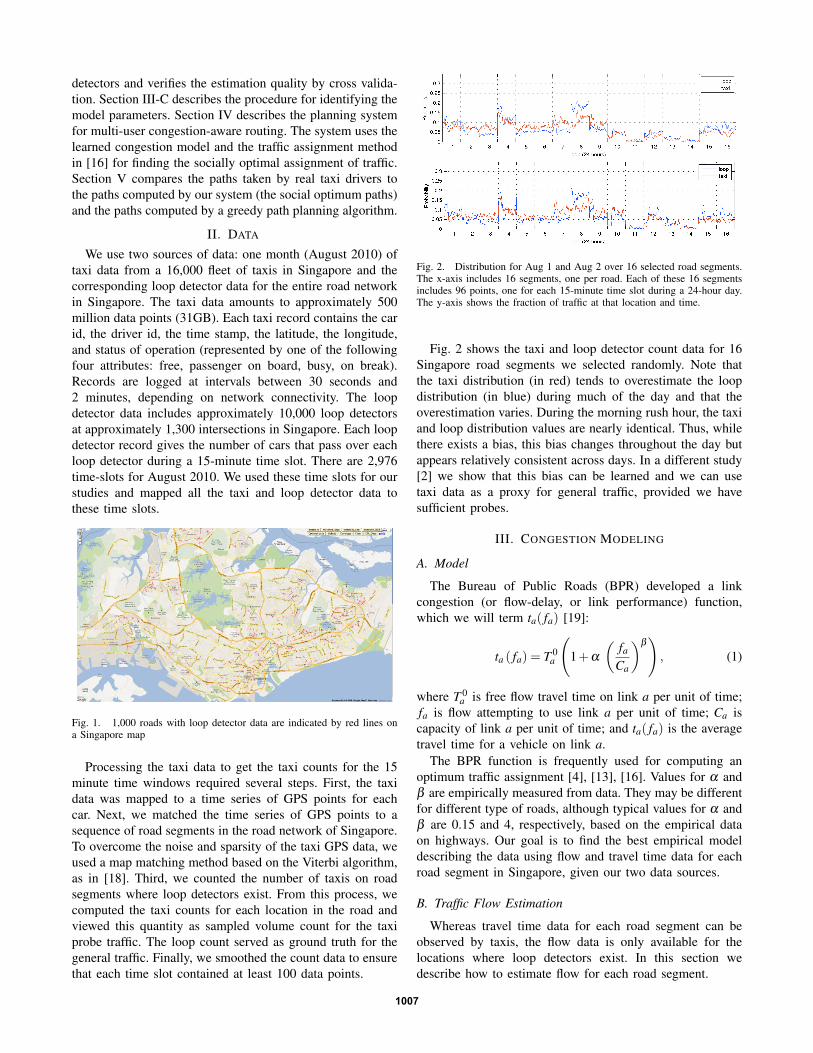
We use two sources of data: one month (August 2010) oftaxi data from a 16,000 fleet of taxis in Singapore and thecorresponding loop detector data for the entire road networkin Singapore. The taxi data amounts to approximately 500million data points (31GB). Each taxi record contains the carid, the driver id, the time stamp, the latitude, the longitude,and status of operation (represented by one of the followingfour attributes: free, passenger on board, busy, on break).Records are logged at intervals between 30 seconds and2 minutes, depending on network connectivity. The loopdetector data includes approximately 10,000 loop detectorsat approximately 1,300 intersections in Singapore. Each loopdetector record gives the number of cars that pass over eachloop detector during a 15-minute time slot. There are 2,976time-slots for August 2010. We used these time slots for ourstudies and mapped all the taxi and loop detector data tothese time slots.

Fig. 1. 1,000 roads with loop detector data are indicated by red lines ona Singapore map

Processing the taxi data to get the taxi counts for the 15minute time windows required several steps. First, the taxidata was mapped to a time series of GPS points for eachcar. Next, we matched the time series of GPS points to asequence of road segments in the road network of Singapore.To overcome the noise and sparsity of the taxi GPS data, weused a map matching method based on the Viterbi algorithm,as in [18]. Third, we counted the number of taxis on roadsegments where loop detectors exist. From this process, wecomputed the taxi counts for each location in the road andviewed this quantity as sampled volume count for the taxiprobe traffic. The loop count served as ground truth for thegeneral traffic. Finally, we smoothed the count data to ensurethat each time slot contained at least 100 data points.

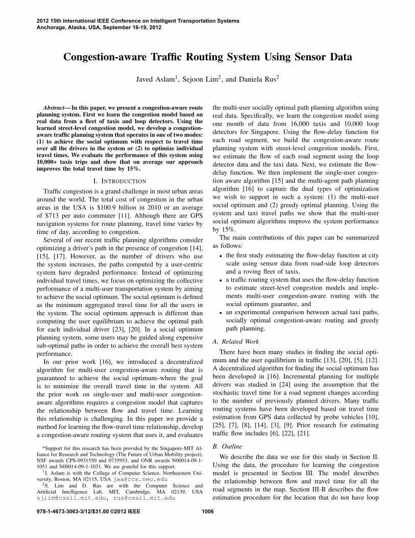
Fig. 2. Distribution for Aug 1 and Aug 2 over 16 selected road segments.The x-axis includes 16 segments, one per road. Each of these 16 segmentsincludes 96 points, one for each 15-minute time slot during a 24-hour day.The y-axis shows the fraction of traffic at that location and time.

Fig. 2 shows the taxi and loop detector count data for 16Singapore road segments we selected randomly. Note thatthe taxi distribution (in red) tends to overestimate the loopdistribution (in blue) during much of the day and that theoverestimation varies. During the morning rush hour, the taxiand loop distribution values are nearly identical. Thus, whilethere exists a bias, this bias changes throughout the day butappears relatively consistent across days. In a different study[2] we show that this bias can be learned and we can usetaxi data as a proxy for general traffic, provided we havesufficient probes.

III. CONGESTION MODELING

A. Model

The Bureau of Public Roads (BPR) developed a linkcongestion (or flow-delay, or link performance) function,which we will term ta( fa) [19]:

ta ( fa) = T 0a

(1+α

(fa

Ca

)β), (1)

where T 0a is free flow travel time on link a per unit of time;

fa is flow attempting to use link a per unit of time; Ca iscapacity of link a per unit of time; and ta( fa) is the averagetravel time for a vehicle on link a.

The BPR function is frequently used for computing anoptimum traffic assignment [4], [13], [16]. Values for α andβ are empirically measured from data. They may be differentfor different type of roads, although typical values for α andβ are 0.15 and 4, respectively, based on the empirical dataon highways. Our goal is to find the best empirical modeldescribing the data using flow and travel time data for eachroad segment in Singapore, given our two data sources.

B. Traffic Flow Estimation

Whereas travel time data for each road segment can beobserved by taxis, the flow data is only available for thelocations where loop detectors exist. In this section wedescribe how to estimate flow for each road segment.

1007

Given a road segment, our goal is to estimate its BPRrelationship using the road’s flow and speed history. Real-time speed can be obtained from the taxi sensor networkeverywhere. However, flow can only be obtained for theroads with loop detectors, but static loop detectors are notavailable for all roads. We develop a computational approachto estimating the flow for locations where the loop data isnot available. Since ground-truth speed is given as the taxispeed, we focus on a method for estimating the flow of theroad.

Let O be the set of all roads with associated loop detectors.Suppose road i does not have an associated loop detector(i /∈ O). Our goal is to estimate the flow for road i usingthe real-time flow data from all the roads with associatedloop detectors O and taxi count information for the road setO∪{i}. Intuitively, we will estimate the flow of road i by theweighted average of flow at other roads with loop detectors,where the weight is defined by the similarity between roadi and a road j in O.

We quantify the similarity between roads i and j by severalmeasures:

• measure 1: m1(i, j) = 1d(i, j) , where d(i, j) is the Eu-

clidean distance between road i and road j• measure 2: m2(i, j) = 1

a(i, j) , where a(i, j) is the angulardifference between the orientation of road i and that ofroad j

• measure 3: m3(i, j)= 1l(i, j) , where l(i, j) is the difference

between number of lanes of road i and that of road j• measure 4: m4(i, j)= 1

t(i, j) , where t(i, j) is the differencebetween taxi count for road i and that of road j

Each of these four measures is an inversely proportionalrelation. Measures 1, 2, and 3 are static. The informationdepends on neither time nor traffic conditions. Measure 4captures the dynamic real-time information observed by taxiprobes.

We define an aggregated similarity measure using the fourmeasures. For a pair of roads i and j, (i, j), the aggregatesimilarity measure is given as follows:

s(i, j) = m1(i, j)u1 ×m2(i, j)u2 ×m3(i, j)u3 ×m4(i, j)u4 (2)

where uk is the indicator for whether measure mk should beconsidered for deciding the aggregate similarity.

uk =

{1 if measure mk should be considered0 otherwise

We choose the best uk empirically.Algorithm 1 describes the method for real-time estimation

of traffic flow f̃ (i) for road i /∈ O, using the real-time loopdetector data from all roads in O. Our algorithm estimates theflow by the weighted average of the available loop detectorcounts for all the roads in O. The weight assigned to eachloop detector on road j for the estimation of flow for roadi, wi( j), is defined as the normalized aggregate similaritymeasure for all the road segments in O as follows:

wi( j) =s(i, j)

∑∀k∈O s(i,k),∃ j ∈ O (3)

The estimation of flow for i, f̃ (i), is calculated as theweighted average of the other observed loop counts usingthe weight wi( j),∀ j ∈ O as follows:

f̃ (i) = ( ft(i)) ∑∀ j∈O, ft ( j)6=0

wi( j)f ( j)ft( j)

(4)

where f ( j) is the observed loop count of road j divided bythe number of lanes of road j.

Algorithm 1: Estimate-FlowData:f ( j): loop count data for road j where loop detectorexists;ft(i): taxi count data for road i;euclidean distance between all pairs of roads;angular difference of orientation between all pairs ofroads;difference in number of lanes between all pairs of roads;difference in taxi count for all pairs of roads;uk: the indicators for each similarity measure;Result: f̃ (i): estimated relative flow for road i without

loop detector1 O = a set of all roads where loop detectors exist ;2 for j ∈ O do3 Find m1(i, j), m2(i, j), m3(i, j), and m4(i, j) ;4 s(i, j) =

m1(i, j)u1 ×m2(i, j)u2 ×m3(i, j)u3 ×m4(i, j)u4 ;5 wi( j) = s(i, j)

∑∀k∈O s(i,k) ,∀ j ∈ O6 end7 f̃ (i) = ( ft(i))∑∀ j∈O wi( j) f ( j)

ft ( j) ;

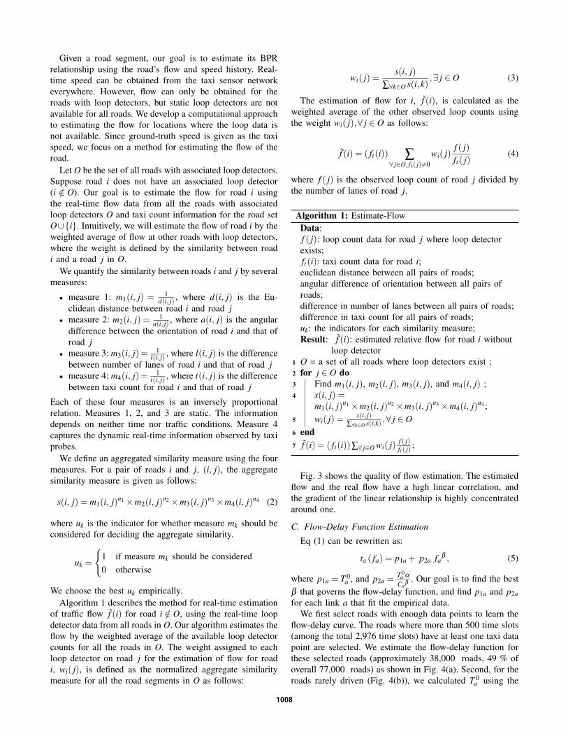
Fig. 3 shows the quality of flow estimation. The estimatedflow and the real flow have a high linear correlation, andthe gradient of the linear relationship is highly concentratedaround one.

C. Flow-Delay Function Estimation

Eq (1) can be rewritten as:

ta ( fa) = p1a + p2a faβ , (5)

where p1a = T 0a , and p2a =

T 0a α

Caβ

. Our goal is to find the bestβ that governs the flow-delay function, and find p1a and p2afor each link a that fit the empirical data.

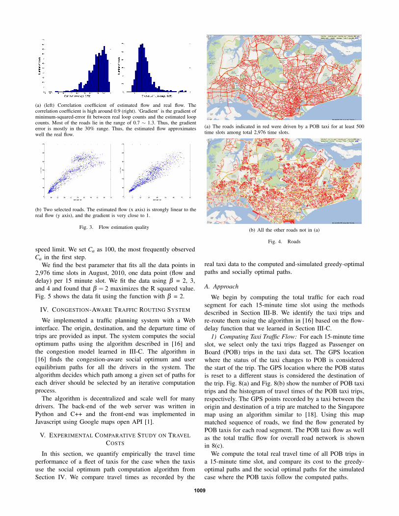
We first select roads with enough data points to learn theflow-delay curve. The roads where more than 500 time slots(among the total 2,976 time slots) have at least one taxi datapoint are selected. We estimate the flow-delay function forthese selected roads (approximately 38,000 roads, 49 % ofoverall 77,000 roads) as shown in Fig. 4(a). Second, for theroads rarely driven (Fig. 4(b)), we calculated T 0

a using the

1008

(a) (left) Correlation coefficient of estimated flow and real flow. Thecorrelation coefficient is high around 0.9 (right). ‘Gradient’ is the gradient ofminimum-squared-error fit between real loop counts and the estimated loopcounts. Most of the roads lie in the range of 0.7 ∼ 1.3. Thus, the gradienterror is mostly in the 30% range. Thus, the estimated flow approximateswell the real flow.

(b) Two selected roads. The estimated flow (x axis) is strongly linear to thereal flow (y axis), and the gradient is very close to 1.

Fig. 3. Flow estimation quality

speed limit. We set Ca as 100, the most frequently observedCa in the first step.

We find the best parameter that fits all the data points in2,976 time slots in August, 2010, one data point (flow anddelay) per 15 minute slot. We fit the data using β = 2, 3,and 4 and found that β = 2 maximizes the R squared value.Fig. 5 shows the data fit using the function with β = 2.

IV. CONGESTION-AWARE TRAFFIC ROUTING SYSTEM

We implemented a traffic planning system with a Webinterface. The origin, destination, and the departure time oftrips are provided as input. The system computes the socialoptimum paths using the algorithm described in [16] andthe congestion model learned in III-C. The algorithm in[16] finds the congestion-aware social optimum and userequilibrium paths for all the drivers in the system. Thealgorithm decides which path among a given set of paths foreach driver should be selected by an iterative computationprocess.

The algorithm is decentralized and scale well for manydrivers. The back-end of the web server was written inPython and C++ and the front-end was implemented inJavascript using Google maps open API [1].

V. EXPERIMENTAL COMPARATIVE STUDY ON TRAVELCOSTS

In this section, we quantify empirically the travel timeperformance of a fleet of taxis for the case when the taxisuse the social optimum path computation algorithm fromSection IV. We compare travel times as recorded by the

(a) The roads indicated in red were driven by a POB taxi for at least 500time slots among total 2,976 time slots.

(b) All the other roads not in (a)

Fig. 4. Roads

real taxi data to the computed and-simulated greedy-optimalpaths and socially optimal paths.

A. Approach

We begin by computing the total traffic for each roadsegment for each 15-minute time slot using the methodsdescribed in Section III-B. We identify the taxi trips andre-route them using the algorithm in [16] based on the flow-delay function that we learned in Section III-C.

1) Computing Taxi Traffic Flow: For each 15-minute timeslot, we select only the taxi trips flagged as Passenger onBoard (POB) trips in the taxi data set. The GPS locationwhere the status of the taxi changes to POB is consideredthe start of the trip. The GPS location where the POB statusis reset to a different staus is considered the destination ofthe trip. Fig. 8(a) and Fig. 8(b) show the number of POB taxitrips and the histogram of travel times of the POB taxi trips,respectively. The GPS points recorded by a taxi between theorigin and destination of a trip are matched to the Singaporemap using an algorithm similar to [18]. Using this mapmatched sequence of roads, we find the flow generated byPOB taxis for each road segment. The POB taxi flow as wellas the total traffic flow for overall road network is shownin 8(c).

We compute the total real travel time of all POB trips ina 15-minute time slot, and compare its cost to the greedy-optimal paths and the social optimal paths for the simulatedcase where the POB taxis follow the computed paths.

1009

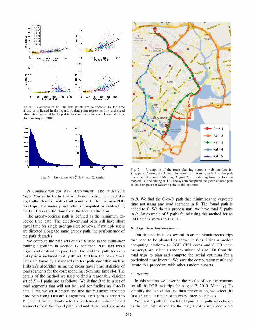
Fig. 5. Goodness of fit. The data points are color-coded by the timeof day as indicated in the legend. A data point represents flow and speedinformation gathered by loop detectors and taxis for each 15-minute timeblock in August, 2010.

Fig. 6. Histogram of T 0a (left) and Ca (right)

2) Computation for New Assignment: The underlyingtraffic flow is the traffic that we do not control. The underly-ing traffic flow consists of all non-taxi traffic and non-POBtaxi trips. The underlying traffic is computed by subtractingthe POB taxi traffic flow from the total traffic flow.

The greedy-optimal path is defined as the minimum ex-pected time path. The greedy-optimal path will have shorttravel time for single user queries; however, if multiple usersare directed along the same greedy path, the performance ofthe path degrades.

We compute the path sets of size K used in the multi-userrouting algorithm in Section IV for each POB taxi trip’sorigin and destination pair. First, the real taxi path for eachO-D pair is included to its path set, P. Then, the other K−1paths are found by a standard shortest path algorithm such asDijkstra’s algorithm using the mean travel time statistics ofroad segments for the corresponding 15-minute time slot. Thedetails of the method we used to find a reasonably disjointset of K−1 paths are as follows: We define B to be a set ofroad segments that will not be used for finding an O-to-Dpath. First, we set B empty and find the minimum expectedtime path using Dijkstra’s algorithm. This path is added toP. Second, we randomly select a predefined number of roadsegments from the found path, and add these road segments

Fig. 7. A snapshot of the route planning system’s web interface forSingapore. Among the 5 paths indicated on the map, path 1 is the paththat a taxi at 8 am on Monday, August 2, 2010 starting from the locationmarked ‘O’ and ending at ‘D’. The system computed the green-colored pathas the best path for achieving the social optimum.

to B. We find the O-to-D path that minimizes the expectedtime not using any road segment in B. The found path isadded to P. We do this process until we have total K pathsin P. An example of 5 paths found using this method for anO-D pair is shows in Fig. 7.

B. Algorithm Implementation

Our data set includes several thousand simultaneous tripsthat need to be planned as shown in 8(a). Using a modestcomputing platform (4 2GH CPU cores and 8 GB mainmemory), we select a random subset of size 100 from thetotal trips to plan and compute the social optimum for apredefined time interval. We save the computation result anditerate this procedure with other random subsets.

C. Results

In this section we describe the results of our experimentsfor all the POB taxi trips for August 2, 2010 (Monday). Tosimplify the exposition and data presentation, we select thefirst 15-minute time slot in every three hour-block.

We used 5 paths for each O-D pair. One path was chosenas the real path driven by the taxi; 4 paths were computed

1010

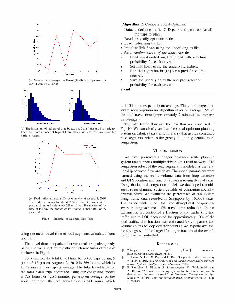
(a) Number of Passenger on Board (POB) taxi trips over theday of August 2, 2010

(b) The histogram of real travel time by taxis at 2 am (left) and 8 am (right).There are more number of trips at 8 am than 2 am, and the travel time fora trip is longer.

(c) Total traffic and taxi traffic over the day of August 2, 2010.Taxi traffic accounts for about 20% of the total traffic at 11pm and 2 am and only about 2% at 11 am. For the rest of thetime of the day, the portion of taxi traffic is about 10% of thetotal traffic.

Fig. 8. Statistics of Selected Taxi Trips

using the mean travel time of road segments calculated fromtaxi data.

The travel time comparison between real taxi paths, greedypaths, and social optimum paths of different times of the dayis shown in Fig. 9.

For example, the total travel time for 3,400 trips during 5pm ∼ 5:15 pm on Auguest 2, 2010 is 769 hours, which is13.58 minutes per trip on average. The total travel time forthe total 3,400 trips computed using our congestion modelis 728 hours, or 12.86 minutes per trip on average. At thesocial optimum, the total travel time is 641 hours, which

Algorithm 2: Compute-Social-OptimumData: underlying traffic, O-D pairs and path sets for all

the trips to plan;Result: socially optimum paths;

1 Load underlying traffic;2 Initialize link flows using the underlying traffic;3 for a random subset of the total trips do4 Load saved underlying traffic and path selection

probability for each driver;5 Set link flows using the underlying traffic.;6 Run the algorithm in [16] for a predefined time

interval;7 Save the underlying traffic and path selection

probability for each driver;8 end

is 11.32 minutes per trip on average. Thus, the congestion-aware social-optmimum algorithm saves on average 15% ofthe total travel time (approximately 2 minutes less per tripon average.)

The total traffic flow and the taxi flow are visualized inFig. 10. We can clearly see that the social optimum planningsystem distributes taxi traffic in a way that avoids congestedroad segments, whereas the greedy solution generates morecongestion.

VI. CONCLUSION

We have presented a congestion-aware route planningsystem that supports multiple drivers on a road network. Thecongestion effect of the road segment is modeled as the rela-tionship between flow and delay. The model parameters werelearned using the traffic volume data from loop detectorsand GPS location and time data from a roving fleet of taxis.Using the learned congestion model, we developed a multi-agent route planning system capable of computing socially-optimal paths. We evaluated the performace of this systemusing traffic data recorded in Singapore by 10,000+ taxis.The experiments show that socially-optimal congestion-aware routing achieves 15% travel time reduction. In ourexeriments, we controlled a fraction of the traffic (the taxitraffic due to POB accounted for approximately 10% of thetotal traffic; this fraction was estimated by comparing taxivolume counts to loop detector counts.) We hypothesize thatthe savings would be larger if a larger fraction of the overalltraffic can be controlled.

REFERENCES

[1] “Google maps api.” [Online]. Available:https://developers.google.com/maps/

[2] J. Aslam, S. Lim, X. Pan, and D. Rus, “City-scale traffic forecastingwith taxi probes,” in The 10th ACM Conference on Embedded NetworkSensor Systems (SenSys12), In Submission, 2012.

[3] P. Borokhov, S. Blandin, S. Samaranayake, O. Goldschmidt, andA. Bayen, “An adaptive routing system for location-aware mobiledevices on the road network,” in Intelligent Transportation Sys-tems (ITSC), 2011 14th International IEEE Conference on, 2011, p.18391845.

1011

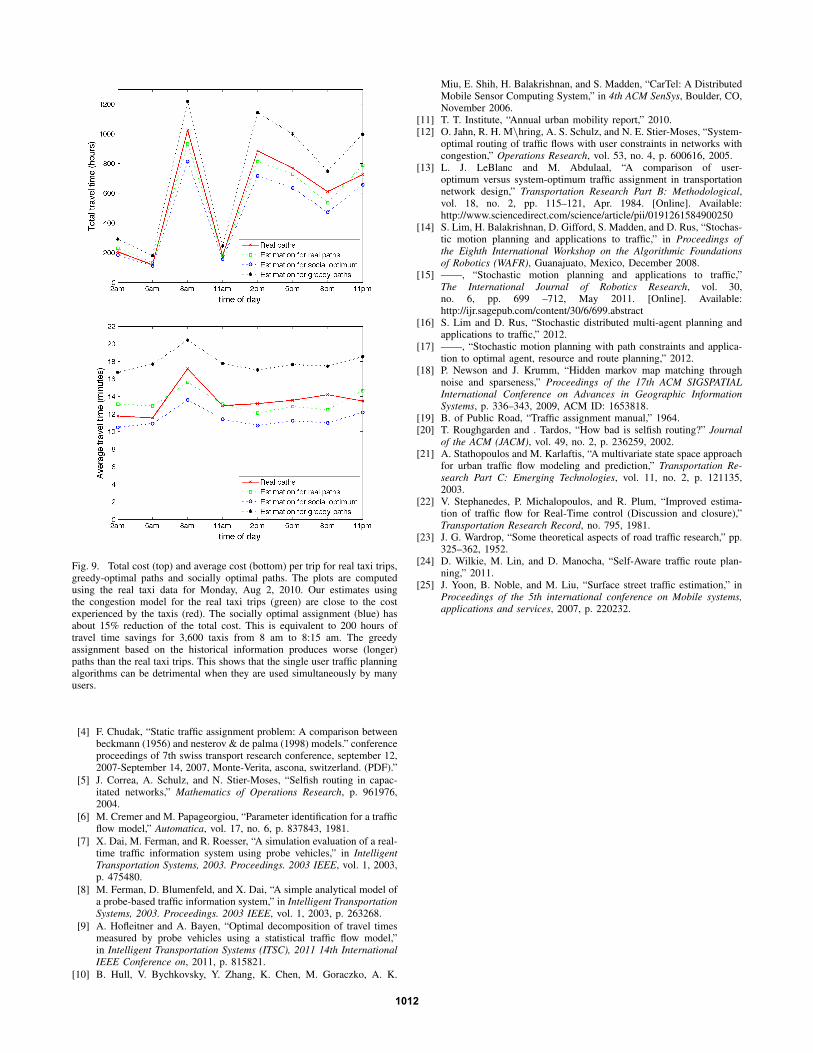
Fig. 9. Total cost (top) and average cost (bottom) per trip for real taxi trips,greedy-optimal paths and socially optimal paths. The plots are computedusing the real taxi data for Monday, Aug 2, 2010. Our estimates usingthe congestion model for the real taxi trips (green) are close to the costexperienced by the taxis (red). The socially optimal assignment (blue) hasabout 15% reduction of the total cost. This is equivalent to 200 hours oftravel time savings for 3,600 taxis from 8 am to 8:15 am. The greedyassignment based on the historical information produces worse (longer)paths than the real taxi trips. This shows that the single user traffic planningalgorithms can be detrimental when they are used simultaneously by manyusers.

[4] F. Chudak, “Static traffic assignment problem: A comparison betweenbeckmann (1956) and nesterov & de palma (1998) models.” conferenceproceedings of 7th swiss transport research conference, september 12,2007-September 14, 2007, Monte-Verita, ascona, switzerland. (PDF).”

[5] J. Correa, A. Schulz, and N. Stier-Moses, “Selfish routing in capac-itated networks,” Mathematics of Operations Research, p. 961976,2004.

[6] M. Cremer and M. Papageorgiou, “Parameter identification for a trafficflow model,” Automatica, vol. 17, no. 6, p. 837843, 1981.

[7] X. Dai, M. Ferman, and R. Roesser, “A simulation evaluation of a real-time traffic information system using probe vehicles,” in IntelligentTransportation Systems, 2003. Proceedings. 2003 IEEE, vol. 1, 2003,p. 475480.

[8] M. Ferman, D. Blumenfeld, and X. Dai, “A simple analytical model ofa probe-based traffic information system,” in Intelligent TransportationSystems, 2003. Proceedings. 2003 IEEE, vol. 1, 2003, p. 263268.

[9] A. Hofleitner and A. Bayen, “Optimal decomposition of travel timesmeasured by probe vehicles using a statistical traffic flow model,”in Intelligent Transportation Systems (ITSC), 2011 14th InternationalIEEE Conference on, 2011, p. 815821.

[10] B. Hull, V. Bychkovsky, Y. Zhang, K. Chen, M. Goraczko, A. K.

Miu, E. Shih, H. Balakrishnan, and S. Madden, “CarTel: A DistributedMobile Sensor Computing System,” in 4th ACM SenSys, Boulder, CO,November 2006.

[11] T. T. Institute, “Annual urban mobility report,” 2010.[12] O. Jahn, R. H. M\hring, A. S. Schulz, and N. E. Stier-Moses, “System-

optimal routing of traffic flows with user constraints in networks withcongestion,” Operations Research, vol. 53, no. 4, p. 600616, 2005.

[13] L. J. LeBlanc and M. Abdulaal, “A comparison of user-optimum versus system-optimum traffic assignment in transportationnetwork design,” Transportation Research Part B: Methodological,vol. 18, no. 2, pp. 115–121, Apr. 1984. [Online]. Available:http://www.sciencedirect.com/science/article/pii/0191261584900250

[14] S. Lim, H. Balakrishnan, D. Gifford, S. Madden, and D. Rus, “Stochas-tic motion planning and applications to traffic,” in Proceedings ofthe Eighth International Workshop on the Algorithmic Foundationsof Robotics (WAFR), Guanajuato, Mexico, December 2008.

[15] ——, “Stochastic motion planning and applications to traffic,”The International Journal of Robotics Research, vol. 30,no. 6, pp. 699 –712, May 2011. [Online]. Available:http://ijr.sagepub.com/content/30/6/699.abstract

[16] S. Lim and D. Rus, “Stochastic distributed multi-agent planning andapplications to traffic,” 2012.

[17] ——, “Stochastic motion planning with path constraints and applica-tion to optimal agent, resource and route planning,” 2012.

[18] P. Newson and J. Krumm, “Hidden markov map matching throughnoise and sparseness,” Proceedings of the 17th ACM SIGSPATIALInternational Conference on Advances in Geographic InformationSystems, p. 336–343, 2009, ACM ID: 1653818.

[19] B. of Public Road, “Traffic assignment manual,” 1964.[20] T. Roughgarden and . Tardos, “How bad is selfish routing?” Journal

of the ACM (JACM), vol. 49, no. 2, p. 236259, 2002.[21] A. Stathopoulos and M. Karlaftis, “A multivariate state space approach

for urban traffic flow modeling and prediction,” Transportation Re-search Part C: Emerging Technologies, vol. 11, no. 2, p. 121135,2003.

[22] V. Stephanedes, P. Michalopoulos, and R. Plum, “Improved estima-tion of traffic flow for Real-Time control (Discussion and closure),”Transportation Research Record, no. 795, 1981.

[23] J. G. Wardrop, “Some theoretical aspects of road traffic research,” pp.325–362, 1952.

[24] D. Wilkie, M. Lin, and D. Manocha, “Self-Aware traffic route plan-ning,” 2011.

[25] J. Yoon, B. Noble, and M. Liu, “Surface street traffic estimation,” inProceedings of the 5th international conference on Mobile systems,applications and services, 2007, p. 220232.

1012

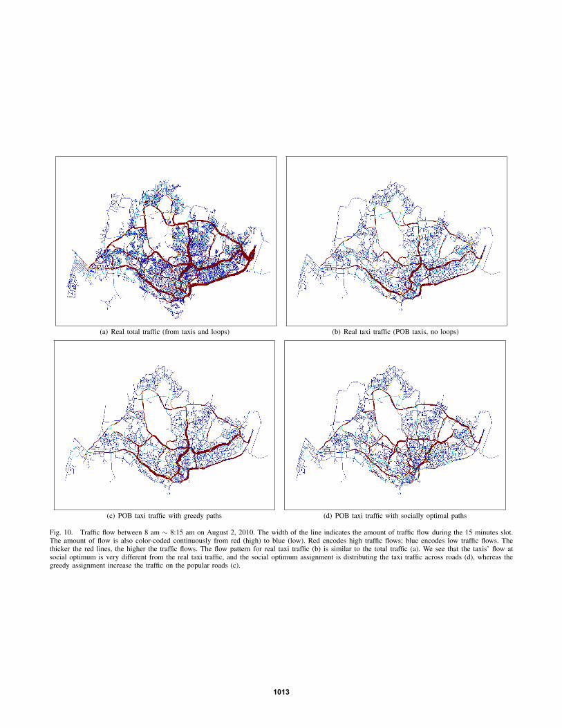
(a) Real total traffic (from taxis and loops) (b) Real taxi traffic (POB taxis, no loops)

(c) POB taxi traffic with greedy paths (d) POB taxi traffic with socially optimal paths

Fig. 10. Traffic flow between 8 am ∼ 8:15 am on August 2, 2010. The width of the line indicates the amount of traffic flow during the 15 minutes slot.The amount of flow is also color-coded continuously from red (high) to blue (low). Red encodes high traffic flows; blue encodes low traffic flows. Thethicker the red lines, the higher the traffic flows. The flow pattern for real taxi traffic (b) is similar to the total traffic (a). We see that the taxis’ flow atsocial optimum is very different from the real taxi traffic, and the social optimum assignment is distributing the taxi traffic across roads (d), whereas thegreedy assignment increase the traffic on the popular roads (c).

1013