Syddansk Universitet

Conformal data of fundamental gauge-Yukawa theories

Dondi, Nicola Andrea; Sannino, Francesco; Prochazka, Vladimir

Published in:Physical Review D

DOI:10.1103/PhysRevD.98.045002

Publication date:2018

Document versionPublisher's PDF, also known as Version of record

Document licenseCC BY

Citation for pulished version (APA):Dondi, N. A., Sannino, F., & Prochazka, V. (2018). Conformal data of fundamental gauge-Yukawa theories.Physical Review D, 98(4), [045002]. DOI: 10.1103/PhysRevD.98.045002

General rightsCopyright and moral rights for the publications made accessible in the public portal are retained by the authors and/or other copyright ownersand it is a condition of accessing publications that users recognise and abide by the legal requirements associated with these rights.

• Users may download and print one copy of any publication from the public portal for the purpose of private study or research. • You may not further distribute the material or use it for any profit-making activity or commercial gain • You may freely distribute the URL identifying the publication in the public portal ?

Take down policyIf you believe that this document breaches copyright please contact us providing details, and we will remove access to the work immediatelyand investigate your claim.

Download date: 12. sep.. 2018

Conformal data of fundamental gauge-Yukawa theories

Nicola Andrea Dondi* and Francesco Sannino†

CP3-Origins & the Danish Institute for Advanced Study DIAS, University of Southern Denmark,Campusvej 55, DK–5230 Odense M, Denmark

Vladimir Prochazka‡

Department of Physics and Astronomy, Uppsala University, Box 516, SE-75120 Uppsala, Sweden

(Received 12 January 2018; published 1 August 2018)

We determine central charges, critical exponents and appropriate gradient flow relations for non-supersymmetric vector-like and chiral Gauge-Yukawa theories that are fundamental according to Wilsonand that feature calculable UV or IR interacting fixed points. We further uncover relations and identitiesamong the various local and global conformal data. This information is used to provide the first extensivecharacterization of general classes of free and safe quantum field theories of either chiral or vector-likenature via their conformal data. Using large Nf techniques we also provide examples in which the safefixed point is nonperturbative but for which conformal perturbation theory can be used to determine theglobal variation of the a central charge.

DOI: 10.1103/PhysRevD.98.045002

I. INTRODUCTION

The standard model is embodied by a gauge-Yukawatheory and constitutes one of the most successful theoriesof nature. It is therefore essential to deepen our under-standing of these theories.An important class of gauge-Yukawa theories is the one

that, according to Wilson [1,2], can be defined fundamental.This means that the theories belonging to this class are validat arbitrary short and long distances. In practice this isensured by requiring that a conformal field theory controlsthe short distance behavior. Asymptotically free theories area time-honoured example [3,4] in which the ultraviolet iscontrolled by a not interacting conformal field theory.Another possibility is that an interacting ultraviolet fixedpoint emerges, these theories are known as asymptoticallysafe. The first proof of existence of asymptotically safegauge-Yukawa theories in four dimensions appeared in [5].The original model has since enjoyed various extensions byinclusion of semisimple gauge groups [6] and supersym-metry [7,8]. These type of theories constitute now animportant alternative to asymptotic freedom. One can nowimagine new extensions of the standard model [9–14] and

novelways to achieve radiative symmetry breaking [9,10]. Infact even QCD and QCD-like theories at large number offlavors can be argued to become safe [15,16] leading to anovel testable safe revolution of the original QCD conformalwindow [17,18].The purpose of this paper is, at first, to determine the

conformal data for generic gauge-Yukawa theories withinperturbation theory. We shall use the acquired informationto relate various interesting quantities characterizing thegiven conformal field theory. We will then specialize ourfindings to determine the conformal data of several funda-mental gauge-Yukawa theories at IR and UV interactingfixed points.The work is organized as follows: In Sec. II we setup the

notation, introduce the most general gauge-Yukawa theoryand briefly summarize the needed building blocks to then inSecs. III and IV determine the explicit expressions inperturbation theory respectively for the local and globalconformal data.We then specialize the results to the case of agauge theory with a single Yukawa coupling in Sec. Vbecause several models are of this type and because it helpsto elucidate some of the salient points of our results. Therelevant templates of asymptotically free and safe fieldtheories are investigated in Sec.VI.Weoffer our conclusionsin Sec. VII. In the Appendices we provide further technicaldetails and setup notation for the perturbative version of thea-theorem and conformal perturbation theory.

II. GAUGE-YUKAWA THEORIES

The classes of theories we are interested in can bedescribed by the following Lagrangian template:

*dondi@cp3.sdu.dk†sannino@cp3.dias.sdu.dk‡vladimir.prochazka@physics.uu.se

Published by the American Physical Society under the terms ofthe Creative Commons Attribution 4.0 International license.Further distribution of this work must maintain attribution tothe author(s) and the published article’s title, journal citation,and DOI. Funded by SCOAP3.

PHYSICAL REVIEW D 98, 045002 (2018)

2470-0010=2018=98(4)=045002(16) 045002-1 Published by the American Physical Society

L ¼ −1

4g2aFμν;aF

μνa þ iΨ†

i σμDμΨi þ

1

2DμϕADμϕA

− ðyAijΨiΨjϕA þ H:c:Þ − 1

4!λABCD ϕAϕBϕCϕD; ð1Þ

where we dropped the gauge indices for Fμν;a, the Weylfermions Ψi the real scalar ϕA and the Yukawa and scalarcoupling matrices. Differently from the notation in [19,20],we make explicit the “flavor” indices, as we have in mindapplication to models containing fields in different gaugegroup representation. The index a runs over the distinctgauge interactions constituting the semisimple gauge groupG ¼ ⊗aGa. The fermions and the scalar transform accord-ing to given representationsRa

ψ iandRa

ϕAof the underlying

simple gauge groups. The Yukawa and scalar couplingstructures are such to respect gauge invariance.In certain cases it is convenient to separate the gauge-

flavor structure of the Yukawa coupling from the couplingitself:

yAij ≡XI

yITIAij ; ð2Þ

where TIAij is a coupling-free matrix and the indices I, j run

on all remaining indices. If flavor symmetries are present,the T matrix will be such to preserve the symmetries. In thisnotation the individual beta functions to the two-loop orderfor the gauge coupling and one-loop for the Yukawas read

βag ¼ −g3a

ð4πÞ2�ba0 þ

ðb1Þabð4πÞ2 g2b þ

ðbyÞaIJð4πÞ2 y

IyJ�; ð3Þ

βIy ¼1

ð4πÞ2 ½ðc1ÞIJKLy

JyKyL þ ðc2ÞbIJ g2byJ�; ð4Þ

where repeated indices [except a in (3)] are summed over.The above beta functions are general with the coefficientsdepending on the specific underlying gauge-Yukawa theory.Furthermore, ðc1ÞIJKL is totally symmetric in the last three(lower) indices as well as ðbyÞaIJ in the Yukawa ones. To thisorder the scalar couplings do not run yet [21]. Therefore tothe present order, that we will refer as the 2-1-0, the d ¼ 4Zamolodchikov two-index symmetric metric χ [cf. (A4)]over the couplings is fully diagonal and reads

χ ¼

χgagag2a

�1þ Aa

ð4πÞ2 g2a

�0

0 χyIyI

!; ð5Þ

where χgg, χyIyI and the Aa quantities are coupling-independent constants. Following Ref. [22] in order toprove that the χyIyJ part of the metric is diagonal we considerthe corresponding operators OI¼Ψ1Ψ2ϕAþðH:cÞ, andOJ ¼ Ψ3Ψ4ϕB þ ðH:cÞ and build the lowest order two-point function

hOIOJiLO ∼ δABðδ13δ24 þ δ23δ14Þ; ð6Þ

which vanishes unless OI ¼ OJ (i.e., when all the indicescoincide). Off-diagonal terms will appear at higher orders.Technically the hOIOJi leading perturbative contribution isa two-loop diagram justifying in (5) the inclusion of the two-loop gauge A-term. Explicitly, in our notation

χgaga ¼1

ð4πÞ2dðGaÞ2

;

χyIyI ¼1

ð4πÞ41

6

XA;i;j

Trg½ðTIAÞijðTIA�Þij�;

Aa ¼ 17CðGaÞ −10

3

Xi

TRaψ i−7

6

Xi

TRaϕi: ð7Þ

The factor of 1ð4πÞ4 in χyIyI agrees with its two-loop nature.

The Weyl consistency conditions, shown to be relevantalso for standard model computations in [20] and furthertested and discussed in [19,23–27], are briefly reviewed inAppendix A (cf. (A7) and (A8) in particular) for the presentsystem and yield the following scheme-independent rela-tions among the gauge and Yukawa coefficients in the betafunctions:

1

ð4πÞ2 χgagaðbyÞaIJ ¼ −χyIyI ðc2ÞaIJ

χyIyI ðc1ÞIJLK ¼ χyJyJðc1ÞJIKLðc2ÞaIJ χyIyI ¼ ðc2ÞaJI χyJyJ

ðb1Þabχgaga ¼ ðb1Þbaχgbgb : ð8Þ

These relations can be used to check or predict the 2-loopcontribution to the gauge beta functions coming from theYukawa interactions once the metric (7) is known.

III. LOCAL QUANTITIES AT FIXED POINTS

Assume that the theory described in (1) admits aninteracting fixed point. This phase of the theory is describedby a CFT characterized by a well defined set of quantities.We loosely refer to this set as the conformal data of theCFT and it includes the critical exponents as well as thequantities a, c, a=c. We refer the reader to Appendix A fordefinitions of central charges a and c. Intuitively suchquantities usually serve as a measure of degrees of freedomin the given CFT. In the present work, these are calculatedusing perturbation theory, so we rely on the assumption thatthe fixed point is not strongly coupled. This is usually undercontrol in the Veneziano limit Nc, Nf → ∞ such that the

ratio Nf

Ncis finite. Moreover, such ratio needs to be close to

the critical value for which the theory loses asymptoticfreedom (which depends on the particular content of thetheory). That is, we have b0 ∝ ϵ for some ϵ being a small

DONDI, SANNINO, and PROCHAZKA PHYS. REV. D 98, 045002 (2018)

045002-2

positive parameter. This ϵ expansion is useful to determinethe local quantities at the fixed point, and reorganize theperturbation theory series in the couplings.

A. a-function at two loops

When Weyl consistency conditions are satisfied we canintegrate the gradient flow equation (A4) to determine thelowest two orders of a¼ að0Þþ að1Þ

ð4πÞ2þ að2Þð4πÞ4þ��� the result is

að0Þ ¼ 1

360ð4πÞ2�nϕ þ

11

2nψ þ 62nv

�;

að1Þ ¼ −1

2

Xa

χgagaba0g

2a;

að2Þ ¼ −1

4

Xa

χgagag2a

��Aaba0g

2a þ

Xb

ðb1Þabg2b�

þXIJ

ðbyÞaIJyIyJ�þ 4π2

XI

χyIyIβIy: ð9Þ

At fixed points ðg�; y�I Þ this quantity becomes scheme-independent and physical and reduces to the so calleda-function [see (A3)]. This quantity partially characterizesthe associated conformal field theory. The interacting fixedpoint requires

ðc2ÞaIJðg�aÞ2y�J ¼ −ðc1ÞIJKLy�Jy�Ky�LðbyÞaIJy�Iy�J ¼ −ðb1Þabðg�bÞ2 − ð4πÞ2ba0 ð10Þ

stemming from βagðg�a;y�I Þ¼βIyðg�a;y�I Þ¼0 with the explicitexpressions given in (3) and (4). We then have the generalexpression

a� ¼ a� ¼ afree −1

4

1

ð4πÞ2Xa

ba0χgagag�2a

�1þ Ag�2a

ð4πÞ2�

þOðg�6a ; y�6I Þ: ð11Þ

The Yukawa couplings do not appear explicitly in the aboveexpression to this order. In the Veneziano limit the lowestorder of a behaves as að1Þ ∼ ϵ2 since ba0 ∼ g�2 ∼ ϵ. The aquantity has to satisfy the bound a > 0 for any CFT. Due tothe fact that in perturbation theory the dominant term is thefree one, positivity is ensured in large N limit such that ϵ isarbitrary small. If the bound happens to be violated, it has tobe interpreted as a failure of perturbation theory to thatgiven order.

B. c-function at two loops

Adapting the two loop results given in [28,29] tothe generic theories envisioned here one derives for c ¼cð0Þð4πÞ2 þ cð1Þ

ð4πÞ4 þ � � � the coefficients

cð0Þ ¼ð4πÞ2cfree¼1

20

�2nvþnψ þ

1

6nϕ

�;

cð1Þ ¼24

�−2

9

Xa

g2adðGaÞ�CðGaÞ−

7

16

Xi

TRaψ i−1

4

XA

TRaϕA

�

−1

24

XI

ðyIÞ2Tr½TITI���; ð12Þ

where TRaψ i, TRa

ϕAare the trace normalization for fermions

and scalars while CðGaÞ is the Casimir of the adjointrepresentation. When this quantity is evaluated at the fixedpoint, it behaves as cð1Þ ∼ ϵ. This order mismatch with awas expected as c does not satisfy a gradient flow equationin d ¼ 4.Like the a quantity, also c is required to satisfy c > 0 at a

fixed point. Within perturbation theory however, the lead-ing order is always positive definite so the violation of thebound is due to failure of the perturbative approach.

C. a=c and collider bounds

Having at our disposal both a and c one can discuss thequantity a

c. It has been shown in [30–33] that the ratio of thecentral charges a and c in d ¼ 4 satisfies the followinginequality

1

3≤ac≤31

18; ð13Þ

which is known as collider bound. Due to the fact thatað1Þ ∼ ϵ2 the next-to-leading order of a=c takes contributionfrom cð1Þ. To calculate the next correction wewould need toknow theOðg4Þ terms in c. Notice that because of this ordermismatch the ratio a

c might become interesting also inperturbation theory for theories living at the edges of thecollider bounds (13). For example free scalar field theorieshave a

c ¼ 13, this implies that for such theories the ϵ order

coefficient has to satisfy að0Þϵ − cð0Þϵ − cð1Þϵ > 0.

D. Scaling exponents

Is it always possible to linearize the RG flow in theproximity of a nontrivial fixed point and thus exactly solvethe flow equation

βiðgiÞ ∼ ∂βi∂gj ðg

j − gj�Þ þOððgj − gj�Þ2Þ

⇒ giðμÞ ¼ gi� þXk

Aikck

�μ

Λ

�θðiÞ ð14Þ

whereμ is theRG scale, ck a is a coefficient depending on theinitial conditions of the couplings,Ai

k is the matrix diagonal-

izing Mij ¼ ∂βi

∂gj and θðiÞ are the corresponding eigenvalues.

These are called critical exponents and from their signs

CONFORMAL DATA OF FUNDAMENTAL GAUGE-YUKAWA … PHYS. REV. D 98, 045002 (2018)

045002-3

one determines if the FP is UV/IR-attractive or mixed. It isworth notice that in the Veneziano limit, Mg

g ∼ ϵ2,MI

g ∼Oðϵ3Þ, meaning that the mixing is not present at thelowest order and we will always have a critical exponent,say, θ1 such that θ1 ∼Mg

g þOðϵ3Þ ∼ ϵ2 þOðϵ3Þ.

IV. GLOBAL PROPERTIES OF RG FLOWSBETWEEN FIXED POINTS

A. Weak a-theorem

Theweak a-theorem states that, given a RG flow betweenaCFTIR andCFTUV, the quantityΔa ¼ aUV − aIR is alwayspositive [34]. This turns out to be a relevant constraint evenin perturbation theory, as the zeroth order leading partcancels out. For example, for an arbitrary semisimple gaugetheory featuring either complete asymptotic freedom orinfrared freedom the Δa variation reads

Δa¼�1

4

1

ð4πÞ2ba0χggg

�2a

�1þAbg�2b

ð4πÞ2�þOðg�6a ;y�6I Þ: ð15Þ

The plus (minus) applies when the theory is asymptoticallyfree (infrared free). The case of the infrared free requires theultraviolet theory to be asymptotically safe. More generally,for single gauge coupling in Veneziano limit jb0j ≪ 1 wecan derive a constraint from the leading order expression

Δa ¼ −1

4

1

ð4πÞ2 b0χggðg�2UV − g�2IRÞ ≥ 0: ð16Þ

Since χgg > 0, from the above inequality we derive therather intuitive constraint that the gauge coupling has toincrease (decrease) with the RG flow in asymptotically free(safe) theories. A less intuitive constraint arises for theoriesfeaturing semisimple gauge groups⊗i¼1;N Gi for which wefind

Δa ¼ −1

4

1

ð4πÞ2XNi¼1

ba0χgagaΔg2a ≥ 0; ð17Þ

where Δg2a ¼ g�2aUV − g�2a IR. From the above we obtain

Xi

dðGiÞba0Δg2a ≤ 0: ð18Þ

No other theorem is known to be valid for flows betweentwo CFTs. For example it is known that Δc, in general, canbe either positive or negative [35]. Let us conclude thissubsection with a comment on the variation of the a

cquantity. If one considers theories living at the edge ofthe collider bound, then within perturbation theory

Δ�ac

�≡ aUV

cUV−aIRcIR

¼ −afreec2free

ΔcþOðϵ2Þ; ð19Þ

must be positive (negative) for the lower (upper) colliderbound. This immediately translates in a bound for the Δcsign. Of course, this is not expected to be valid beyondperturbation theory, while Δa > 0 was proven to hold evennonperturbatively [34].

B. Weakly relevant flows at strong coupling

It is useful to discuss Δa in the context of “conformalperturbation theory,” which allows one to extend theperturbative analysis to potentially strongly coupled theo-ries. The basic idea behind conformal perturbation theory isutilizing small deformation of CFT to study how does thebehavior close to fixed point depend on the its conformaldata. We will the assume existence of an interacting (notnecessarily weakly coupled) CFT in the UV and induce anRG flow by adding a slightly relevant coupling deformation.Utilizing this language we will derive the relation betweenΔa of weakly relevant flows and critical exponents.To set up the nomenclature we will consider a flow close

to an arbitrary UV fixed point (denoted by CFTUV)described by a set of N couplings giUV. We will deformthe CFTUV slightly by Δgi with jΔgj≡ ðΔgiÞ2 ≪ 1 andassume, that within this regime there exists another fixedpoint giIR corresponding to CFTIR. More concretely we willassume the existence of (diagonalized) beta functions in thevicinity of the fixed point [cf. (B3)]

βi ¼ θðiÞΔgi þ cijkΔgjΔgk þOðΔg3Þ ð20Þwhere θðiÞ correspond to critical exponents in the diagon-alized basis of coupling space and cijk are related to the OPEcoefficients of associated nearly-marginal operators. In thefollowing we will assume the existence of a nearby IR fixedpoint with Δg� such that βiðΔg�Þ ¼ 0þOðΔg3Þ. A smallΔgi solution exists if θðiÞ ∼ ϵ ≪ 1 for generic some smallparameter ϵ (not necessarily equal to the Venezianoparameter) so that Δg� ∼ ϵ.1 Expanding the a- functionclose to g

UVwe get

aIR ¼ aUV þ Δgi∂iajgUV

þ 1

2ΔgiΔgj∂i∂jajg

UV

þ 1

6ΔgiΔgjΔgk∂i∂j∂kajg

UVþOðΔg4Þ: ð21Þ

Next we will use the relation [see (A4)]

∂ia≡ ∂∂gi a ¼ βjχij; ð22Þ

where the metric χij is positive close to fixed point [22,36]and we have assumed the one-form wi is exact close to a

1Note that if cijk is small (like it is the case in weakly coupledgauge theories), we need to expand βi to higher orders in orders tofind a zero.

DONDI, SANNINO, and PROCHAZKA PHYS. REV. D 98, 045002 (2018)

045002-4

fixed point2 The Eq. (22) also explains why we need toexpand a up to ðΔgÞ3. This is because the beta functions(20) are Oðϵ2Þ, so we expect their contribution to a tobe Oðϵ3Þ.Using (22) and the fact that beta functions have to vanish

at the UV fixed point it is clear that the leading correctionterm [OðΔgÞ in (21)] vanishes and the we are left with

aIR ¼ aUV þ 1

2ΔgiΔgjχkj∂iβ

kjgUV

þ 1

6ΔgiΔgjΔgkχil∂j∂kβ

ljgUV

þ 1

6ΔgiΔgjΔgk∂kχil∂jβ

ljgUV

þOðΔg4Þ: ð23Þ

Note that the term proportional to ∂χ is Oðϵ4Þ, hence byusing (20) we get

aIR ¼ aUV þ 1

2Δgi�Δgj�χijθðiÞ þ

1

3Δgi�Δgj�Δgk�χilcljk

þOðϵ4Þ: ð24Þ

Now applying the fixed point condition βiðΔg�Þ ¼ 0we get

aIR ¼ aUV þ 1

6Δgi�Δgj�χijθðiÞ þOðϵ4Þ; ð25Þ

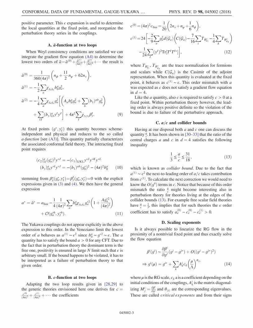
where we see that the OPE coefficients cljk dropped out atthis order, so that the final result (25) only depends on thecritical exponents.Let us explore the RG flow close to UV fixed point (see

Fig. 1). In between the nearby fixed points, the renormal-ized trajectory can be described by a line joining the fixedpoints. In known cases (e.g., [5]), this line is parallel to thedirection corresponding to relevant eigenvector as indicatedin Fig. 1. If this is the case Δg is an eigenvector of the UVstability matrix ∂iβ

kjgUV

and we clearly have

Δg�iΔg�jχijθðiÞ ¼ θUVrel: ðΔg�iÞ2χii; ð26Þ

where θUVrel: ≡ θðiÞ is the critical exponent correspondingto the respective relevant direction on Fig. 1. Thereforeplugging this back into (25) we deduce

aIR ¼ aUV þ 1

6θUVrel: ðΔg�iÞ2χii þOðΔg3Þ: ð27Þ

Since θUVrel: corresponds to a relevant direction it has to benegative so together with the positivity of χij it implies thatto leading order the correction

Δa ¼ Δa ¼ aUV − aIR ≈ −1

6θUVrel: ðΔg�iÞ2χii > 0; ð28Þ

consistently with the a-theorem.The above result can be straightforwardly extended to

the case with multiple relevant couplings since we do notexpect irrelevant directions to contribute to (25).We are now ready to provide the conformal data

associated to distinct classes of asymptotically free or safequantum field theories.

V. THE SINGLE YUKAWA THEORY

We start with analysing the general model templatefeaturing a simple gauge group and one Yukawa coupling.In the perturbation theory one can draw general conclusionson the phase diagram structure. At the 2-1-0 loop level twokinds of fixed points can arise: one in which both gauge andYukawa couplings are nonzero (denoted as GY fixed pointin the following) and a Banks-Zaks fixed point, where thegauge coupling is turned on while the Yukawa is zero(denoted as BZ fixed point). The control parameter ϵ in theVeneziano limit3 is identified such that b0 ∼ Ncϵ, with Ncthe number of colors. These theories have the followinggeneral system of β-functions

βg ¼ −g3

ð4πÞ2�b0 þ b1

g2

ð4πÞ2 þ byy2

ð4πÞ2�

βy ¼y

ð4πÞ2 ½c1y2 þ c2g2� ð29Þ

for which the following fixed points are present

�g2�GYð4πÞ2¼−

b0b1e

;y2�GYð4πÞ2¼

c2c1

b0b1e

� �g2�BZð4πÞ2¼−

b0b1

;y2�BZð4πÞ2¼0

�

ð30Þ

FIG. 1. RG flow close to UV fixed point gUV

≡ ðg1UV;…gNUVÞ.The thick black line represents the renormalized trajectorybetween two fixed points, which is parallel to the relevant direction(red arrow). Irrelevant directions correspond to blue arrows.

2This has been observed in all of the known examples. Mostnotably in perturbation theory close to a Gaussian fixed point in[37] and for supersymmetric theories in [38]. In two dimensionswi was proven to be exact [39].

3This limit is strictly speaking applicable when consideringSUðNcÞ gauge theories with matter in the fundamentalrepresentation.

CONFORMAL DATA OF FUNDAMENTAL GAUGE-YUKAWA … PHYS. REV. D 98, 045002 (2018)

045002-5

where b1e ¼ b1ð1 − byb1

c2c1Þ. The above ϵ-expansion of the

fixed point couplings is reliable only up to Oðϵ2Þ, wherethese higher orders are modified by higher loop corrections.These fixed points can be physical or not depending on thesigns of the various beta function parameters.We will now calculate the conformal data for this general

template to the leading 2-1-0 order. This corresponds totruncating every quantity to the first nontrivial order in the ϵexpansion.

A. Scaling exponents

The scaling exponents at each fixed point are determinedby diagonalizing the rescaled flow matrix Mij ¼ 1

Nc

∂βi∂gj.These read

(i) BZ fixed point

θ1¼−2b20b1

∼Oðϵ2Þ; θ2¼−c2b0b1

∼OðϵÞ ð31Þ

The corresponding eigendirections are

v1 ¼�1

0

�v2 ¼

�0

1

�ð32Þ

And are thus parallel to the gauge-Yukawa couplingaxis. Notice how the gauge coupling runs slowerwith respect to the Yukawa one, which thereforereaches asymptotic freedom much faster.

(ii) GY fixed point: In general c1 > 0 and c2 < 0 [40]

θ1 ¼ −2b20b1e

∼Oðϵ2Þ; θ2 ¼ c2b0b1

∼OðϵÞ ð33Þ

While the eigendirections are

v1 ¼

0B@

1ffiffiffiffiffiffiffi1−c2

c1

p − b0c1

ffiffiffiffiffiffiffiffiffiffiffið1−c2

c1Þ3

p þOðϵ2Þ1ffiffiffiffiffiffiffi1−c1

c2

p − c1b0c22

ffiffiffiffiffiffiffiffiffiffiffið1þc1

c2Þ3

p þOðϵ2Þ

1CA

v2 ¼

0B@

byb0b1effiffiffiffiffiffiffiffiffi−c1c2

p þOðϵ2Þ

1þ b2yb202c1c2b21e

þOðϵ3Þ

1CA ð34Þ

Notice that as ϵ → 0 the flow between the GY fixedpoint and the Gaussian one becomes a straight lineon the v1 direction, forming an angle α with the gaxis such that tanðαÞ ¼ − c1

c2. In this case a solution tothe fixed flow equation is present. Moreover, sinceα ∈ ½0; π=2� we see that if the GY fixed point ispresent then such a solution always exists, while theconverse may not be true.The eigencoupling along the direction of each

eigenvector enjoys a power scaling close to the fixed

point as in (14), and the associated operator defor-mations then become either relevant or irrelevantdepending on the sign of scaling exponents at thefixed point.

B. Determining a, c and the collider bound

For the single gauge-Yukawa system (29) we can use theexpressions (9),(12) to determine the a,c functions at fixedpoint. Notice that the A coefficient has the expected Ncdependence A ∼ Nc. However, since the fixed point isknown only to OðϵÞ at two loop level, the A term can beneglected since it only contributes to Oðϵ3Þ. We have

(i) GY point

a� ¼ a� ¼ afree −1

4χggb0

g�2GYð4πÞ2

¼ afree −1

8χggθ

GY1 þOðϵ3Þ; ð35Þ

c ¼ cfree þ�u − v

c2c1

�b0b1

þOðϵ2Þ ð36Þ

ac¼ aF

cF

�1 −

1

cF

�u − v

c2c1

�b0b1

þOðϵ2Þ�

ð37Þ

(ii) BZ point

a� ¼ a� ¼ afree −1

4χggb0

g�2BZð4πÞ2

¼ afree −1

8χggθ

BZ1 þOðϵ3Þ; ð38Þ

c ¼ cfree þ ub0b1

ϵþOðϵ2Þ ð39Þ

ac¼ aF

cF

�1 −

ucF

b0b1

þOðϵ2Þ�: ð40Þ

It is seen that for both of the above fixed points the two-loop contribution to the a− function is proportional to thescaling exponent with the highest power in ϵ

Δa ¼ aFP − afree ¼ −1

8χggθ

FPg þOðϵ3Þ: ð41Þ

The critical exponent in the above equation corresponds tothe eigendirection pointing towards the Gaussian fixedpoint, which is coherent with our discussion in Sec. IV Bfor strongly coupled fixed points. This implies that for RGflows where one of the fixed points is Gaussian, we findagain that Δa is proportional to a scaling exponent.

DONDI, SANNINO, and PROCHAZKA PHYS. REV. D 98, 045002 (2018)

045002-6

VI. RELATED FREE AND SAFEMODEL TEMPLATES

In the following we will calculate the local quantities forfixed point arising in different Gauge-Yukawa theories. Weare interested in flows between an interacting fixed pointand the Gaussian one. Depending on which point is theCFTUV these are either free or safe UV complete theories.We will consider these cases separately and provideexamples for each one of them.

A. Asymptotically free theories

1. Vectorlike SU(N) gauge-fermion theory

Consider an SU(N) gauge theory with vectorlike fer-mions and its N ¼ 1 SYM extension, the field content issummarized in Table I. The supersymmetric extension ofthe model can be fitted into our gauge-Yukawa templateintroducing the following Yukawa interaction for eachchiral field

L ¼�ψa λA

��0

ffiffiffi2

pgTA

abffiffiffi2

pgTA

ab 0

��ψa

λA

�ϕb þ H:c:

ð42Þ

These theories feature a Banks-Zaks fixed point arisingat 2-loop level. The relevant beta function coefficients areknown

bN¼00 ¼ 2

3Ncϵ; bN¼0

1 ¼ −25

2N2

c þOðϵÞ;

ϵ ¼112Nc − Nf

Nc> 0;

bN¼10 ¼ Ncϵ; bN¼1

1 ¼ −6N2c þOðϵÞ;

ϵ ¼ 3Nc − Nf

Nc> 0: ð43Þ

Results are summarized in Table II.4

Additionally we have the expressions for globalquantities

ΔaN¼0 ¼ N2c

ð4πÞ21

255ϵ2 þOðϵ3Þ; ð45Þ

ΔaN¼1 ¼ N2c

ð4πÞ21

48ϵ2 þOðϵ3Þ; ð46Þ

TheN ¼ 0 agrees with the original result of [37]. We see atleading order the a-theorem does not provide any stronglimits on ϵ so one might expect the higher orders will bemore restrictive. However the recent Oðϵ4Þ evaluation ofΔaN¼0 in [42] reveals that to this order all the subleadingcoefficients remain to be positive providing no furtherperturbative bounds on ϵ.

2. Complete asymptotically free vectorlike gaugetheories with charged scalars

Consider the scalar-gauge theory analyzed in [43] withmatter content presented in Table III. Such model can beseen as the extension of the vectorlike SU(N) gauge theoryas well as the result of SUSY breaking of the N ¼ 1version with a scalar remnant. This model has no Yukawacouplings as they are forbidden by gauge invariance. The

TABLE I. Field content of the vectorlike SUðNÞ gauge theory.The lower table contains the superpartners of the N ¼ 1extension.

Fields ½SUðNcÞ� SULðNfÞ SURðNfÞAμ Adj 1 1ψ □ □ 1ψ □ 1 □

λ Adj 1 1ϕ □ □ 1ϕ □ 1 □

TABLE II. Results for N ¼ 0, 1 gauge theories.

ϵNcg2

ð4πÞ2 θg a × ð4πÞ2N2

cc × ð4πÞ2

N2c

a=c

N ¼ 0 112− Nf

Nc

4ϵ75

16ϵ2

22549144

− 11ϵ360

− ϵ2

225288320

þ 19ϵ80

245468

− 1933ϵ8112

N ¼ 1 3 − Nf

Nc

ϵ6

ϵ2

3516− ϵ

24− ϵ2

4838− ϵ

2456− ϵ

54

TABLE III. Field content of the model in [43].

Fields ½SUðNcÞ� SULðNfÞ SURðNfÞ UðNsÞψ □ □ 1 1ψ □ 1 □ 1ϕ □ 1 1 □

4The SUSY results of Table II are readily confirmed by usingthe exact SUSY formulas [41]

c ¼ 1

32

1

ð4πÞ2 ½4dðGÞ þ dðriÞð9ðR − 1Þ3 − 5ðR − 1ÞÞ�

a ¼ 3

32

1

ð4πÞ2 ½2dðGÞ þ dðriÞð3ðR − 1Þ3 − ðR − 1ÞÞ� ð44Þ

with R ¼ 23− ϵ

9being the perturbative R-charge of squark field at

the fixed point.

CONFORMAL DATA OF FUNDAMENTAL GAUGE-YUKAWA … PHYS. REV. D 98, 045002 (2018)

045002-7

scalar field features a self-interaction in the form of theusual single and double trace potentials

L ¼ −vTr½ϕ†ϕ�2 − uTr½ðϕ†ϕÞ2� ð47Þ

It has been shown that this model features completeasymptotic freedom when an infrared fixed point is present.We analyze the flow between such point, when it exists, andthe free UV one. At 2-1-1 loop level the fixed point splitsinto two denoted as FP1, FP2 due to the presence of thescalar self-couplings and both of these are featuring a flowto the Gaussian fixed point. In Fig. 2 we plot theperturbative central charges of these fixed points fordifferent vectorlike flavors and colors. We focus on theminimal case realizing such fixed point, with number ofcomplex scalars Ns ¼ 2. Notice that the central charges areevaluated at the two-loop level, so no distinction is presentbetween FP1 and FP2 [20]. We observe that the mostsensitive quantity, as function of the number of flavors, isa=c, which fails to satisfy the lower bound a=c > 1=3 forsufficiently low number of flavors. Δa is, however, alwayssmall and positive and spans several orders of magnitude.In Table IV we calculate positions of the fixed points andtheir critical exponents for the model in the large-Nc, Nf

limit of the model, where the central charges are identical tothe ones on the first line of Table II.

3. Complete asymptotically free chiralgauge-Yukawa theories

A further generalization of the previous models isobtained by adding chiral and vectorlike fermions in higherdimensional representation of the gauge group (seeTable V). In particular we consider the models in[44,45], namely the generalized Georgi-Glashow [46]and Bars-Yankielowicz models [47] which are by con-struction gauge anomaly free. We will work in the large Nclimit tuning the constant x ¼ p=Nc, so that these twotheories are described by the same set of β-functions. Attwo-loop level this theory resembles the template discussedin Sec. V where both BZ and GY fixed points are present.

(i) BZ fixed point.This type of fixed point arises for 3

2< x < 9

2where

at the lower limit it becomes nonperturbative and at

a c

FIG. 2. a-function (upper left), c-function (upper right), collider bound a=c (lower left) and Δa (lower right) between the IR fixedpoint and the Gaussian.

TABLE IV. Fixed points position and critical exponents in theVeneziano limit for the couplings of the theory.

Ncg�2

ð4πÞ2 u�Nf=ð4πÞ2 v�N2f=ð4πÞ2 θðiÞ

FP1 4ϵ75 −121

300ð9−4 ffiffiffi

6p Þϵ 11

150ð3− ffiffiffi

6p Þϵ 16

225ϵ2, −

ffiffi23

q8ϵ25, −

ffiffi23

q8ϵ25

FP2 4ϵ75 −121

300ð9þ4

ffiffiffi6

p Þϵ 11150

ð3þ ffiffiffi6

p Þϵ 16225

ϵ2,ffiffi23

q8ϵ25,

ffiffi23

q8ϵ25

DONDI, SANNINO, and PROCHAZKA PHYS. REV. D 98, 045002 (2018)

045002-8

the upper one it merges with the Gaussian fixedpoint. We will thus expand around the perturbativeedge of the x-window (also known as conformalwindow in the literature), namely write x ¼ 9

2− ϵ

and arrive at the following fixed point

Ncg2BZð4πÞ2 ¼ 2

39ϵþOðϵ2Þ; Ncy2BZ

ð4πÞ2 ¼ 0: ð48Þ

At this fixed point we have the following set ofeigendirection and critical exponents

θ1 ¼8

117ϵ2 þOðϵ3Þ θ2 ¼ −

4

13ϵþOðϵ2Þ

v1 ¼�1

0

�v2 ¼

� 11ϵ26

1 − 121ϵ2

1352

�ð49Þ

as well as the central charges values

a ¼ N2c

ð4πÞ2�289

720−

7ϵ

120−

7ϵ2

4680

�þOðϵ3Þ

c ¼ N2c

ð4πÞ2�91

160þ 1193ϵ

6240

�þOðϵ2Þ

a=c ¼ 578

819−987670ϵ

2906631þOðϵ2Þ

Δa ¼ aFREE − aBZ ¼ N2c

ð4πÞ2ϵ2

234þOðϵ3Þ ð50Þ

(ii) GY fixed point.This is present for 3

8ð3þ ffiffiffiffiffi

61p Þ < x < 9

2and it

behaves similarly to the BZ fixed point close to theupper and lower limits of the x window. Workingclose to the upper edge of the conformal windowx ¼ 9

2− ϵ we obtain

Ncg2GYð4πÞ2 ¼ 16

15ϵþOðϵ2Þ;

Ncy2BZð4πÞ2 ¼ 8

15ϵþOðϵ2Þ ð51Þ

at which we have the following set of eigendirectionand critical exponents

θ1 ¼64

45ϵ2 þOðϵ3Þ θ2 ¼

32

5ϵþOðϵ2Þ

v1 ¼

0B@

ffiffi45

q− 7ϵ

75ffiffi5

pffiffi15

qþ 14ϵ

45ffiffi5

p

1CA v2 ¼

� − 445ϵ

1 − 96825

ϵ2

�ð52Þ

The central charges are now

a ¼ N2c

ð4πÞ2�289

720−

7ϵ

120−31ϵ2

360

�þOðϵ3Þ

c ¼ N2c

ð4πÞ2�91

160þ 761ϵ

120

�þOðϵ2Þ

a=c ¼ 579

819−1782364ϵ

223587þOðϵ2Þ

Δa ¼ aFREE − aGY ¼ N2c

ð4πÞ24ϵ2

45þOðϵ3Þ ð53Þ

One can notice that a flow between the two non-trivial fixed points is present, in which the BZ fixedpoint can be viewed as the UV completion of the GYone. This is supported by the positivity of Δabetween these two points

Δa ¼ aBZ − aGY ¼ N2c

ð4πÞ211ϵ2

130: ð54Þ

B. Safe models

The discovery of asymptotic safety in four dimensions[5] has triggered much interest. It is therefore timely toinvestigate the associated conformal data.

1. SU(N) with Nf fundamental flavorsand (gauged) scalars

We start with the original theory that we will refer to, inthe following, as LS theory [5] that features the fieldcontent summarized in the Table VI and the Lagrangian

LY ¼ yψϕψ þ H:c:

LS ¼ −uTr½ðϕ†ϕÞ2� − vðTr½ϕ†ϕ�Þ2 ð55Þ

As before at 2-1-0 order we will only focus on Yukawacoupling, keeping Nc, Nf large. This time we will consider

0 < Nf−112Nc

Nc¼ ϵ ≪ 1, slightly above the asymptotic free-

dom bound. Such theory possesses an UV fixed point [5].In the Veneziano limit the coefficients of (29) read

b0¼−2

3ϵNc; b1¼−

�25

2−13

3ϵ

�N2

c;

by ¼121

4N2

cþOðϵÞ; c1¼13

2NcþOðϵÞ; c2 ¼−3Nc:

ð56Þ

TABLE V. Field content of the Georgi-Glashow/Bars-Yankielowicz models.

Fields ½SUðNcÞ� SUðNc ∓ 4þ pÞ SUðpÞψ □ 1 □

ψ □ □ 1A=S 1 1

CONFORMAL DATA OF FUNDAMENTAL GAUGE-YUKAWA … PHYS. REV. D 98, 045002 (2018)

045002-9

Therefore we have b1e ¼ 1913N2

c, which leads to the follow-ing UV fixed point [5]

�Ncg�2

ð4πÞ2 ¼ 26

57ϵ;Ncy�2

ð4πÞ2 ¼ 12

57ϵ

�: ð57Þ

The critical exponents yield

θ1 ¼ −2b20b1e

¼ −104

171ϵ2; θ2 ¼ 2c2

b0b1e

¼ 52

19ϵ; ð58Þ

corresponding to the eigendirections

v1 ¼

0B@

ffiffiffiffi1319

qffiffiffiffi619

q1CA; v1 ¼

�0

1

�: ð59Þ

The a function at this fixed point is given by

aLS ¼ afree −1

4

χggð4πÞ4 b0g

�2

¼ afree þ13N2

c

342

1

ð4πÞ2 ϵ2

¼ 1

ð4πÞ2N2

c

120

�61þ 11ϵþ 298ϵ2

57

�: ð60Þ

Next we will proceed to calculate cLS

cLS ¼ cfree þ31N2

c

68

1

ð4πÞ2 ϵ

¼ N2c

ð4πÞ21

120

�211

2þ 2ϵ

17þOðϵ2Þ

�: ð61Þ

Note we would need to know the Oðg4; y4Þ contribution toc, in order to determine the Oðϵ2Þ correction of the a=cquantity that to order ϵ reads:

aLScLS

¼ 122

211þ 78426ϵ

756857þOðϵ2Þ: ð62Þ

Notice that the collider bound is well satisfied as long asϵ≲ 1. Using the general result obtained in Sec. A 1 it ispossible to obtain the 3-loop expression forΔa between theUV safe fixed point and the Gaussian one in the IR:

Δa¼ N2c

ð4πÞ2�13

342ϵ2þ

�65201− 11132

ffiffiffiffiffi23

p

246924

�ϵ3�þOðϵ4Þ:

ð63ÞEven at finite Nc and Nf asymptotic safety abides the localand global constraints as long as the ϵ parameter iscontrollably small.Recently, this model has been extended [11] to accom-

modate a gauged Higgs-like scalar (in fundamental repre-sentation) and 2Nf singlet fermions Ni, N0i (see Table VII).This theory has some extra Yukawa and scalar couplings

LY ¼ yψϕψ þ y0NH†N0 þ yHψN þ y0H†ψN0 þ H:c:

LS ¼ −λS1Tr½ϕ†ϕ�2 − λS2Tr½ðϕ†ϕÞ2� − λHðH†HÞ2− λHSðH†HÞTr½ϕ†ϕ� ð64Þ

Note that beta functions of these 3 new Yukawa couplingsdecouple in the Veneziano limit. The fixed point found

in [11] appears at y0� ¼ y0� ¼ 0 and Ncy�2

ð4πÞ2 ¼ ϵ26. Since at the

2-1-0 level βg;y doesn’t depend on y, the model enjoys theLS critical exponents (57) with the third one being

θ3 ¼∂∂y βy

g�;y�;y�

¼ 6

13ϵ; ð65Þ

which corresponds to an extra irrelevant direction in thecoupling space.Clearly the a-function of this model is identical to the LS

one since both models have the same b0 [cf. (11)]. Similarlythe c− function of this model is identical to the LS one.This is due to the fact that the extra contribution of y in (12)is proportional to TrðTyT �

yÞ ∝ NcNf which is suppressed inthe Veneziano limit compared to the g, y contributionproportional to TrðTyT�

yÞ ∝ NcN2f so we can neglect it.

2. Complete asymptotically safe chiral models

The UV dynamics of Georgi-Glashow (GG) models thatinclude also singlet as well as charged scalar fields wasinvestigated in [45].The field content is summarized in Table VIII and

the interactions between chiral fermions and scalars aredescribed via the following Lagrangian terms

TABLE VI. Field content of the LS model.

½SUðNcÞ� SUðNfÞL SUðNfÞRψ □ □ 1ψ □ 1 □

ϕ 1 □ □

TABLE VII. Field content of the model of [11].

Fields ½SUðNcÞ� SUðNfÞL SUðNfÞRψ □ □ 1ψ □ 1 □

ϕ 1 □ □

H □ 1 1N 1 1 □

N0 1 □ 1

DONDI, SANNINO, and PROCHAZKA PHYS. REV. D 98, 045002 (2018)

045002-10

LH ¼ yHfaψaAH þ H:c:

LM ¼ yM½δab − fafb�ψaMbcψc þ y1fafbψaMbcψc þ H:c:

ð66Þ

Where fa is a vector in flavor space. The Higgs-like scalarbreaks the flavor symmetry with the Yukawa term yH. Inthe following we choose to have just one flavor interactingwith the H field, so fa ¼ δa;1. The distinction between yM,y1 is convenient as loop corrections will differentiatebetween the flavor interacting with H with the others. Itis possible to show that the Bars-Yankielowicz (BY)5

version of the theory cannot lead to complete asymptoticsafety for anyNc. Within the GG, the fully interacting FP ofthis theory at 2-1-0 loop level is fully IR attractive in thelarge Nc limit. However there are some candidates of finiteNc theories for which complete asymptotic safety canpotentially emerge. We now determine the conformal datafor the three candidate fixed points found in the originalwork, these are shown in Table IX.We find that all these UV fixed points, at least in some of

the couplings, are clearly outside the perturbative regimegiven that a=c and Δa constraints are not respected.

C. Flows between interacting fixed points

Here we would like to consider models possessinginteracting fixed points in both IR and UV. In the followingwe will investigate the a-theorem constraints to furthercharacterize such flows.

1. BZ-GY flow in the completelyasymptotically free regime

Let us now turn to a class of theories with

b0 > 0; b1 < 0; b1e < 0: ð67Þ

The main features of these models were discussed in Sec. V.We also refer the reader to [40] for a more detaileddiscussion. A concrete example can be realized by coupling

the LS model (c.f. Sec. VI B 1) to some additional fermionsin the adjoint representation (see Table X). Clearly, if theconditions (67) are satisfied, both GY and BZ fixed points[cf. (30)] can coexist. Furthermore if c2 < 0, the BZ fixedpoint acquires a relevant direction corresponding to theYukawa coupling (see (31). It is therefore reasonable toexpect, that there is an RG flow between BZ and GY points.Indeed, using (16) we find that for a generic gauge theorywith group G [recall that χgg ¼ 1

214π2

dðGÞ] we have

Δa ¼ aBZ − aGY ¼ −1

8dðGÞ b

20

b21

byc2c1�

1 − byb1

c2c1

� ; ð68Þ

which is positive since b1e < 0 implies

byc2c1

< b1 < 0: ð69Þ

More concretely we can take an extension of the modeldescribed in Sec. VI B 1 with an extra gluinolike adjointfermion. The relevant beta function coefficients in theVeneziano limit read

b0 ¼2

3ϵNc; b1 ¼−

27

2N2

c; by ¼81

4;

ϵ¼92Nc−Nf

Nc> 0; c1 ¼

11

2NcþOðϵÞ; c2 ¼−3Nc:

ð70Þ

TABLE VIII. Field content of the Georgi-Glashow modelsextended with singlet and charged scalars.

Fields ½SUðNcÞ� SUðNc ∓ 4þ pÞ SUðpÞψ □ 1 □

ψ □ □ 1A 1 1

M 1 □ □

H □ 1 1

TABLE IX. couplings, critical exponents and central chargesfor fixed points that can realize complete asymptotic safety(CAS).

Nc ¼ 5, p ¼ 26 Nc ¼ 6, p ¼ 30 Nc ¼ 8, p ¼ 39

α�g 1.41 0.0325 0.0481α�H 6.12 0.151 0.241α�M 0.652 0.0155 0.0233α�1 0.312 0.00652 0.00801θUV −0.0428 −0.00585 −0.00602a × ð4πÞ2 −1311 14.7 21.6c × ð4πÞ2 710 47.5 126a=c −1.84 0.296 0.171Δa −1321 −0.537 −4.27

TABLE X. Field content of the LS model with an additionaladjoint Weyl fermion.

Fields ½SUðNcÞ� SUðNfÞL SUðNfÞRψ □ □ 1ψ □ 1 □

ϕ 1 □ □

λ Adj 1 1

5The difference with respect to the Georgi-Glashow theories isthat the Weyl fermion transforming according to the two-indexantisymmetric tensor under the gauge group is replaced by asymmetric one.

CONFORMAL DATA OF FUNDAMENTAL GAUGE-YUKAWA … PHYS. REV. D 98, 045002 (2018)

045002-11

For this model b1e ¼ − 2711N2

c and hence it satisfies thecomplete asymptotic safety criterion with two fixed points

Ncg2GYð4πÞ2 ¼ 22

81ϵþOðϵ2Þ; Ncg2BZ

ð4πÞ2 ¼ 4

81ϵþOðϵ2Þ ð71Þ

The flow between these two fixed point (where BZ playsthe role of UV fixed point) satisfies the a-theorem (68)

Δa ¼ 1

ð4π2Þϵ2N2

c

54; ð72Þ

which is positive as expected from the above discussion.

2. Large Nf safety with the Higgs:

Recently an interesting class of large Nf models withstrongly-coupled UV fixed point has been discussed in theliterature [10,12,13]. These models extend previous work[16,48] by including the Higgs and therefore provide arealistic framework for asymptotically safe extensions ofthe standard model. Further insights on the nature andconsistence of these fixed points were investigated in [15].Here we consider a model with large Nf vector-like

fermions and a Higgs-like scalar transforming according tothe fundamental representation of SUðNcÞ. The fieldcontent of this theory is summarized in the Table XI.Expanding to leading order in 1

Nf, the gauge beta function of

this theory has a zero at

A� ¼ Nfg�2

ð4πÞ2 ¼ 3þ ð� � �Þe−NfNc: ð73Þ

The presence of the Higgs self-coupling λH does not disturbthis fixed point at this order in 1

Nf[10] (up to exponentially

suppressed contributions). At one loop the gauge couplingappears without powers of Nf in the quartic beta function,which is therefore under perturbative control. To make thecalculation more manageable we can also take the inter-mediate large Nc limit provided [15]

1

10>

Nc

Nf≫

1

Nf: ð74Þ

Thus given we keep NcNf

small enough, this regime is

attainable. To keep track of 1Nf

in the scalar sector we

introduce the coupling uH ¼ λHNf

ð4πÞ2 with the following beta

function (close to the above UV fixed point A → A�)

βuH ¼1

Nf

�4Ncu2H−6NcuHA� þ3

4NcA�2þO

�1

N2f

;1

Nc

��:

ð75Þ

Thus we see that this beta function remains small if we keepNf large enough. Neglecting the subleading contributionswe have

βuH ¼ 4Nc

NfðuH − uþÞðuH − u−Þ; ð76Þ

where

u� ¼ ð3�ffiffiffi6

pÞ A�

4Nf: ð77Þ

This allows for two fixed points with stable Higgs potentialsince u� > 0. Furthermore, u− is fully UV-attractive sincethe corresponding critical exponent satisfies6

θu− ¼ ∂∂uH βuH

u−

¼ −4Nc

Nfðuþ − u−Þ ¼ −2

ffiffiffi6

p Nc

NfA�

¼ −6ffiffiffi6

p Nc

Nf< 0: ð78Þ

By deforming the scalar coupling away from the fixed pointδuH ¼ ðuH − u−Þ > 0 and keeping the gauge couplingfixed, we expect the theory to flow to a new (also stronglycoupled) IR fixed point at uH ¼ uþ. We are now ready tocompute Δa for this flow using (28) and the leading largeNf behavior of the metric χ

χuHuH ¼ 1

24

�Nc

Nf

�2 1

ð4πÞ2 þO�

1

N3f

�: ð79Þ

Plugging the quantities (77)–(79) directly into (28) weobtain the final result

Δa ¼ −1

6χuHuHθu−ðuþ − u−Þ2 þO

�1

N4f

�

¼ 1

ð4πÞ2�Nc

Nf

�3 9

ffiffiffi6

p

16þO

�1

N4f

�: ð80Þ

TABLE XI. Field content of the model.

Fields ½SUðNcÞ� SUðNfÞL SUðNfÞRψ □ □ 1ψ □ 1 □

ϕ 1 □ □

H □ 1 1

6Note that the critical exponent corresponding to gaugecoupling is always negative irrespectively of the presence ofscalar.

DONDI, SANNINO, and PROCHAZKA PHYS. REV. D 98, 045002 (2018)

045002-12

Note that the smallness of Δa is controlled by NcNf, which is

kept small.

VII. CONCLUSIONS

We provided explicit expressions for the central chargesand critical exponents in perturbation theory for a genericweakly coupled gauge-Yukawa theory. The conformal dataare naturally divided into local quantities characterizing aspecific CFT and global data which are defined over theentire RG flow in between two CFTs belonging to thesame underlying QFT. The local quantities are criticalexponents, central charges and the ratio a=c of two centralcharges. The variation of the central a-charge over the RGgroup defines the globally defined quantity. We charac-terized via their conformal data a wide class of funda-mental (i.e., either free or safe) nonsupersymmetricquantum field theories dynamically developing CFTs at theend points of their perturbative RG flows. These theoriesare both vector and chiral like and constitute the backboneof phenomenologically interesting fundamental extensionsof the standard model. Additionally our results can also beused as independent tests of the perturbative control overthe possible existence of CFTs. We noted that the positivityof a and the conformal collider bound (13) are the mostsensitive criteria. In contrast the positivity of the c chargedoes not provide strong constraints (similar observationwas made in the supersymmetric case in [49]).Interestingly we show that at leading orders in perturbationtheory the global variation of the a charge is proportionalto the critical exponent related to the relevant direction.This means that to this order one has one less independentconformal data. Moreover, we extended this result beyondthe cases in which the specific CFTs are achievedperturbatively by making use of conformal perturbationtheory provided the two CFTs are nearby in couplingspace. Using 1=Nf resummation techniques we alsoconstructed an explicit example in which a stronglycoupled safe CFT emerges that can be investigated usingconformal pertrubation theory for which we can determineΔa. Interestingly this theory features an Higgs-like stateand constitutes the template on which novel asymptoticallysafe standard model extensions have been constructed[10,12,13,15].

ACKNOWLEDGMENTS

The CP3-Origins centre is partially funded by the DanishNational Research Foundation, Grant No. DNRF90. Wethank Kasper Langæble, Esben Mølgaard, Colin Poole andZhi-Wei Wang for useful discussions. V. P. would like tothank CP3-Origins for hospitality during initial and finalstages of this work. V. P. was supported by the EuropeanResearch Council Starting Grant No. 639220 (curvedsusy)during the final stages of the project.

APPENDIX A: PERTURBATIVE A-THEOREM

The matrix element on the vacuum state of the trace ofthe energy–momentum tensor for the metric γμν for ageneral QFT in d ¼ 4 reads

hTμμi ¼ cW2ðγμνÞ − aE4ðγμνÞ þ � � � ; ðA1Þ

where a and c are real coefficients, E4ðγμνÞ the Eulerdensity and WðγμνÞ the Weyl tensor. The dots representcontributions coming from operators that can be con-structed out of the fields defining the theory. Their con-tribution is proportional to the β functions of theircouplings. The coefficient a is the one used in Cardy’sconjecture, and for a free field theory it is [50]

afree ¼1

90ð8πÞ2�nϕ þ

11

2nψ þ 62nv

�; ðA2Þ

where nψ , nψ and nv are respectively the number of realscalars, Weyl fermions and gauge bosons.The change of a along the RG flow is directly related to

the underlying dynamics of the theory via the β functions.This can be shown by exploiting the abelian nature of thetrace anomaly which leads to the Weyl consistency con-ditions in much the same manner as the well known Wess-Zumino consistency conditions [51]. Following the work ofJack and Osborn [22,37], rather than using a one uses thefunction a related to it by

a ¼ aþ wiβi; ðA3Þ

where wi is a one–form which depends on the couplings ofthe theory. The Weyl consistency conditions imply for a

∂ia ¼ −χijβj þ ð∂iwj − ∂jwiÞβj; ðA4Þ

where χij can be viewed as a metric in the space ofcouplings gi. The positivity of the metric χ is established inperturbation theory, and therefore in this regime thefunction a is monotonic along the RG flow

μdadμ

¼ βi∂ia ¼ −χijβiβj ≤ 0: ðA5Þ

The irreversibility of the RG flow has been conjectured tobe valid beyond perturbation theory at least in d ¼ 4.For a generic gauge-Yukawa theory, the functionwi turns

out to be an exact one-form at the lowest orders inperturbation theory [37], so that the terms involvingderivatives of wi cancel out, and we will use in thefollowing the simplified consistency condition

∂a∂gi ¼ −βi; βi ≡ χijβ

j: ðA6Þ

CONFORMAL DATA OF FUNDAMENTAL GAUGE-YUKAWA … PHYS. REV. D 98, 045002 (2018)

045002-13

χij can be seen as a metric in the space of couplings, used inthis case to raise and lower latin-indices. The fact that all βfunctions can be derived from the same quantity a hasprofound implications. The flow generated by the modifiedβ functions βi is a gradient flow, implying in particular

∂βj∂gi ¼

∂βi∂gj ; ðA7Þ

which gives relations between the β functions of differentcouplings. In the case of coupling-independent and diago-nal metric, this relation reduces to

χii∂jβi ¼ χjj∂iβ

j; ðA8Þ

where no summation on i, j is present. These consistencyconditions, known as Weyl consistency conditions can beused as a check of a known computation. In principle theycan also be used to determine some unknown coefficients ata higher loop order in perturbation theory.

1. a beyond two loops

Is it possible to go beyond the two-loop calculation for thea function previously introduced. For simplicitywe considera theory with one gauge group, one Yukawa interaction andtwo couplings in the scalar potential. In this case we canexpress our result in terms of αi ¼ g2i =ð4πÞ2 to get a morecompact notation. We will consider the scalar to be charged

under the gauge group, generalizing the result in [20]. Thetheory is described by the general β-function system

βαg=ð−2α2gÞ ¼ b0 þ b1αg þ byαy þ b3α2g þ b4αgαy þ b5α2y

þ b6αλ1 þ b7αλ1αg þ b8α2λ1 ðA9Þ

þ b9αλ2 þ b10αλ2αg þ b11α2λ2 þ b12αλ1αλ2;

ðA10Þ

βαy=ð2αyÞ ¼ c1αy þ c2αg þ c3αgαy þ c4α2g þ c5α2y

þ c6αyαλ1 þ c7α2λ1 þ c8αλ1αg ðA11Þ

þ c9αyαλ2 þ c10α2λ2 þ c11αλ2αg þ c12αλ1αλ2 ;

ðA12Þ

βαλ1 ¼ d1α2λ1 þ d2αλ1αy þ d3α2y þ d4α2g

þ d5αgαλ1 þ d6α2λ2 þ d7αyαλ2

þ d8αgαλ2 þ d9αλ1αλ2 : ðA13Þ

βαλ2 ¼e1α2λ2 þe2αλ2αyþe3α2yþe4α2gþe5αgαλ2

þe6α2λ1 þe7αyαλ1 þe8αgαλ1 þe9αλ1αλ2 : ðA14Þ

The Zamolodchidov metric is then generalized to

χ ¼

0BBBBB@

χggα2gð1þ Aαg þ B1α

2g þ byαgαy þ B5αgαλ1 þ B6αgαλ2Þ B0 E0 F0

B0χyyαyð1þ B3αy þ B4αgÞ 0 0

E0 0 χλ1λ1 F1

F0 0 F1 χλ2λ2

1CCCCCA: ðA15Þ

The coefficient χgg enters at the one-loop order, A and χyy at two loops, while χλλ and the Bi’s appear only at three loops.New nonzero mixing terms are introduced in accordance with the definition of χ as a function of the 2-point function ofstress-energy tensor. Similarly, the one-form W reads

Wg ¼1

αgðD0 þD1αg þ C1α

2g þ C2αgαy þ C5αgαλ1 þ C6αgαλ2Þ;

Wy ¼ D2 þ C3αy þ C4αg;

Wλ1 ¼ D3αλ1 þD4αg þD5αλ2 :

Wλ2 ¼ E3αλ2 þ E4αg þ E5αλ1 : ðA16Þ

The general structure of χ confirms that it is sufficient for all our purposes to consider the Yukawa β function (A12)to two-loop order and the quartic one (A13), (A14) to one-loop only. The a function is then derived up to three looporder

DONDI, SANNINO, and PROCHAZKA PHYS. REV. D 98, 045002 (2018)

045002-14

aðαiÞ ¼ −1

3χgg

�4b0αg þ α22ðb1 − 3AbyÞ þ 2Ab1α3g þ ðb4 þ 3AbyÞα2gαy þ 4b5αgα2y þ

c1c2

�4b5 − b4

c1c2

�α3y −

1

αgβαg

�

þ 1

3χyy

�1

3c1α2y þ

2

3c2αgαy −

�2

�c1c2

�c3 þ

1

2

�c1c2

�2

ðAc2 − 2c4Þ�α3y − 2c3α2yαg − 2c4αyα2g þ βαy

�

þ 1

3χλ1λ1αλ1βαλ1 þ

1

3χλ2λ2αλ2βαλ2 þ

βαgα2g

fðα3i Þ −β2αy4αy

B0 − C2 þ C4

c2

þ 1

3ðD5 − E5 þ F1Þαλ2βαλ1 −

1

3ðD5 − E5 − F1Þαλ1βαλ2

where we defined

fðα3i Þ ¼2

3E0α

2gαλ1 þ

2

3F0α

2gαλ2 þ χgg

�B1

3α3g þ

by2α2gαy −

by6

�c1c2

�2

α3y þB5

3α2gαλ1 þ

B6

3α2gαλ2

�

þ B0 þ C2 − C4

3

�c1c2

�2

α3y ðA17Þ

the a-function coincides with this expression evaluatedat a fixed point. As expected, all off diagonal terms in themetric and coefficients of the unphysical quantityW drop atfixed point. Additionally all the dependence on scalardynamics drops at a fixed point; every scalar beta functioncoefficient can be rearranged to form a beta function termusing the Weyl consistency conditions. This is not acci-dental: it happens also at 2-1-0 level for the Yukawacoefficients, as shown in the previous section. We canthen predict that the sector that is evaluated at the lowestorder in perturbation theory does not explicitly contributeto the a-function. Nevertheless, it will still contribute to thefixed point values of the gauge and Yukawa couplingsrespectively.

APPENDIX B: CONFORMALPERTURBATION THEORY

In this set-up we will consider a (strongly-)coupled CFT,which is described by the set of nearly marginal primaryoperators Oi with small anomalous dimensions (criticalexponents) Δi ¼ 4þ θðiÞ and the corresponding OPE(operator product expansion)

OiðyÞOjðxÞ ¼x→y ckijjx − yjΔiþΔj−Δk

OkðxÞ þ � � � ; ðB1Þ

where dots correspond to operators of higher spin etc. Wenow proceed to deform the CFT by adding weakly relevantcouplings fλig

SCFT → SCFT þ λiZ

d4xOi: ðB2Þ

Assuming small perturbations with jλij ≪ 1 we will havethe corresponding beta functions

βi ¼ θðiÞλi þ π2Xjk

cijkλjλk þOðλ3Þ: ðB3Þ

This reasoning can be reversed to obtain the conformal datafrom the knowledge of beta functions close to a fixed pointas was done for example in [52,53]

θðiÞ ¼∂∂λi β

i

λi�; cijk ¼

1

2π2∂2

∂λk∂λj βi

λi�: ðB4Þ

It should be noted that the above relation to compute OPEcoefficients is strictly speaking only valid in the diagonalbasis (for a more detailed discussion of this issue seeSec. II. 3 in [52]). For nearly marginal flows with small θðiÞ,there is a possibility of Wilson-Fisher-like IR fixed pointwith small λi�.

[1] K. G. Wilson, Phys. Rev. B 4, 3174 (1971).[2] K. G. Wilson, Phys. Rev. B 4, 3184 (1971).[3] D. J. Gross and F. Wilczek, Phys. Rev. D 8, 3633 (1973).[4] H. D. Politzer, Phys. Rev. Lett. 30, 1346 (1973).

[5] D. F. Litim and F. Sannino, J. High Energy Phys. 12 (2014)178.

[6] A. D. Bond and D. F. Litim, Phys. Rev. D 97, 085008(2018).

CONFORMAL DATA OF FUNDAMENTAL GAUGE-YUKAWA … PHYS. REV. D 98, 045002 (2018)

045002-15

[7] A. D. Bond and D. F. Litim, Phys. Rev. Lett. 119, 211601(2017).

[8] B. Bajc, N. A. Dondi, and F. Sannino, J. High Energy Phys.03 (2018) 005.

[9] S. Abel and F. Sannino, Phys. Rev. D 96, 056028 (2017).[10] S. Abel and F. Sannino, Phys. Rev. D 96, 055021 (2017).[11] G. M. Pelaggi, F. Sannino, A. Strumia, and E. Vigiani,

Front. Phys. 5, 49 (2017).[12] R. Mann, J. Meffe, F. Sannino, T. Steele, Z.-W. Wang, and

C. Zhang, Phys. Rev. Lett. 119, 261802 (2017).[13] G. M. Pelaggi, A. D. Plascencia, A. Salvio, F. Sannino, J.

Smirnov, and A. Strumia, Phys. Rev. D 97, 095013 (2018).[14] A. D. Bond, G. Hiller, K. Kowalska, and D. F. Litim, J. High

Energy Phys. 08 (2017) 004.[15] O. Antipin and F. Sannino, Phys. Rev. D 97, 116007 (2018).[16] C. Pica and F. Sannino, Phys. Rev. D 83, 035013 (2011).[17] F. Sannino and K. Tuominen, Phys. Rev. D 71, 051901

(2005).[18] D. D. Dietrich and F. Sannino, Phys. Rev. D 75, 085018

(2007).[19] I. Jack and C. Poole, J. High Energy Phys. 01 (2015) 138.[20] O. Antipin, M. Gillioz, E. Mølgaard, and F. Sannino, Phys.

Rev. D 87, 125017 (2013).[21] O. Antipin, M. Gillioz, J. Krog, E. Mølgaard, and F.

Sannino, J. High Energy Phys. 08 (2013) 034.[22] H. Osborn, Phys. Lett. B 222, 97 (1989).[23] A. D. Bond, D. F. Litim, G. M. Vazquez, and T. Steudtner,

Phys. Rev. D 97, 036019 (2018).[24] I. Jack and C. Poole, Phys. Rev. D 95, 025010 (2017).[25] A. V. Bednyakov and A. F. Pikelner, Phys. Lett. B 762, 151

(2016).[26] I. Jack, D. R. T. Jones, and C. Poole, J. High Energy Phys.

09 (2015) 061.[27] E. Mølgaard, Eur. Phys. J. Plus 129, 159 (2014).[28] I. Jack, J. Phys. A 16, 1083 (1983).[29] H. Osborn and A. Stergiou, J. High Energy Phys. 06 (2016)

079.[30] D. M. Hofman and J. Maldacena, J. High Energy Phys. 05

(2008) 012.[31] A. Parnachev and S. S. Razamat, J. High Energy Phys. 07

(2009) 010.

[32] Z. Komargodski, M. Kulaxizi, A. Parnachev, and A.Zhiboedov, Phys. Rev. D 95, 065011 (2017).

[33] D. M. Hofman, D. Li, D. Meltzer, D. Poland, and F.Rejon-Barrera, J. High Energy Phys. 06 (2016) 111.

[34] Z. Komargodski and A. Schwimmer, J. High Energy Phys.12 (2011) 099.

[35] A. Cappelli, D. Friedan, and J. I. Latorre, Nucl. Phys. B352,616 (1991).

[36] F. Baume, B. Keren-Zur, R. Rattazzi, and L. Vitale, J. HighEnergy Phys. 08 (2014) 152.

[37] I. Jack and H. Osborn, Nucl. Phys. B343, 647 (1990).[38] R. Auzzi and B. Keren-Zur, J. High Energy Phys. 05 (2015)

150.[39] J. Gomis, P.-S. Hsin, Z. Komargodski, A. Schwimmer, N.

Seiberg, and S. Theisen, J. High Energy Phys. 03 (2016)022.

[40] C. Pica, T. A. Ryttov, and F. Sannino, Phys. Rev. D 96,074015 (2017).

[41] D. Anselmi, J. Erlich, D. Z. Freedman, and A. A. Johansen,Phys. Rev. D 57, 7570 (1998).

[42] V. Prochazka and R. Zwicky, Phys. Rev. D 96, 045011(2017).

[43] F. F. Hansen, T. Janowski, K. Langaeble, R. B. Mann, F.Sannino, T. G. Steele, and Z.-W. Wang, Phys. Rev. D 97,065014 (2018).

[44] T. Appelquist, Z.-y. Duan, and F. Sannino, Phys. Rev. D 61,125009 (2000).

[45] E. Mølgaard and F. Sannino, Phys. Rev. D 96, 056004(2017).

[46] H. Georgi, H. R. Quinn, and S. Weinberg, Phys. Rev. Lett.33, 451 (1974).

[47] I. Bars and S. Yankielowicz, Phys. Lett. 101B, 159 (1981).[48] B. Holdom, Phys. Lett. B 694, 74 (2010).[49] S. P. Martin and J. D. Wells, Phys. Rev. D 64, 036010

(2001).[50] M. J. Duff, Nucl. Phys. B125, 334 (1977).[51] J. Wess and B. Zumino, Phys. Lett. 37B, 95 (1971).[52] A. Codello, M. Safari, G. P. Vacca, and O. Zanusso, Eur.

Phys. J. C 78, 30 (2018).[53] A. Codello, M. Safari, G. P. Vacca, and O. Zanusso, Phys.

Rev. D 96, 081701 (2017).

DONDI, SANNINO, and PROCHAZKA PHYS. REV. D 98, 045002 (2018)

045002-16