Confidence Intervals for Uncommon but Dramatic Responses to Treatment

Confidence Intervals for Uncommon but Dramatic Responses to TreatmentAuthor(s): Paul R. RosenbaumSource: Biometrics, Vol. 63, No. 4 (Dec., 2007), pp. 1164-1171Published by: International Biometric SocietyStable URL: http://www.jstor.org/stable/4541471 .

Accessed: 28/06/2014 10:45

Your use of the JSTOR archive indicates your acceptance of the Terms & Conditions of Use, available at .http://www.jstor.org/page/info/about/policies/terms.jsp

.JSTOR is a not-for-profit service that helps scholars, researchers, and students discover, use, and build upon a wide range ofcontent in a trusted digital archive. We use information technology and tools to increase productivity and facilitate new formsof scholarship. For more information about JSTOR, please contact [email protected].

.

International Biometric Society is collaborating with JSTOR to digitize, preserve and extend access toBiometrics.

http://www.jstor.org

This content downloaded from 193.142.30.103 on Sat, 28 Jun 2014 10:45:47 AMAll use subject to JSTOR Terms and Conditions

http://www.jstor.org/action/showPublisher?publisherCode=ibs

http://www.jstor.org/stable/4541471?origin=JSTOR-pdf

http://www.jstor.org/page/info/about/policies/terms.jsp


BIOMETRICS 63, 1164-1171 DOI: 10.1111/j.1541-0420.2007.00783.x December 2007

Confidence Intervals for Uncommon but Dramatic Responses to Treatment

Paul R. Rosenbaum

Department of Statistics, The Wharton School, University of Pennsylvania, Philadelphia, Pennsylvania 19104-6340, U.S.A.

email: [email protected]

SUMMARY. A small literature discusses locally most powerful rank tests when only a fraction of treated subjects respond to treatment. The ranks used in these tests are very different from conventional ranks, being relatively flat for low responses and then rising steeply, and the associated tests are much more powerful than conventional rank tests when, indeed, only a small fraction of treated subjects exhibit dramatic responses. Because the tests are derived from considerations of local power, they do not yield a plausible family of models for effect, and therefore they do not yield confidence intervals for the magnitude of effect formed by inverting the tests. There is a similarity between these tests and another family of tests, originally motivated by different considerations involving peak performance in small subsets. Exploiting this similarity, a method for obtaining confidence statements is proposed. In the case of observational studies, sensitivity to unobserved bias from nonrandom assignment of treatments is also examined. Two examples are used as illustrations: (i) a study of smoking during pregnancy and its effects on birth weight, in which smokers are matched to six controls, and (ii) a matched pair study of damage to DNA among workers at aluminum production plants.

KEY WORDS: Attributable effects; Causal effects; Observational study; Sensitivity analysis.

1. Introduction 1.1 Example: Smoking During Pregnancy and Birth Weight

Using data from the National Institute on Drug Abuse's

"Washington, DC Metropolitan Area Drug Study (DC*MADS)," Figure 1 depicts the birth weights in

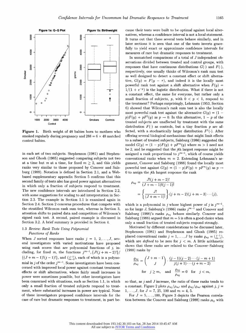
grams of 48 babies born to mothers who smoked regularly during pregnancy and 288 = 6 x 48 matched control babies born to mothers who did not smoke during pregnancy. None of these mothers reported using illicit drugs or drinking alcohol regularly during pregnancy. The 48 smokers were each matched to six nonsmokers for two variables, whether or not the mother was on Medicaid, and whether or not the mother received regular prenatal care (i.e., at least once a

month). Of the smokers, 46 of 48 reported smoking less than a pack a day and 2 of 48 reported smoking at least a pack a

day; however, it is not clear how accurate these self-reports of amount smoked are. On the left in Figure la, there is a

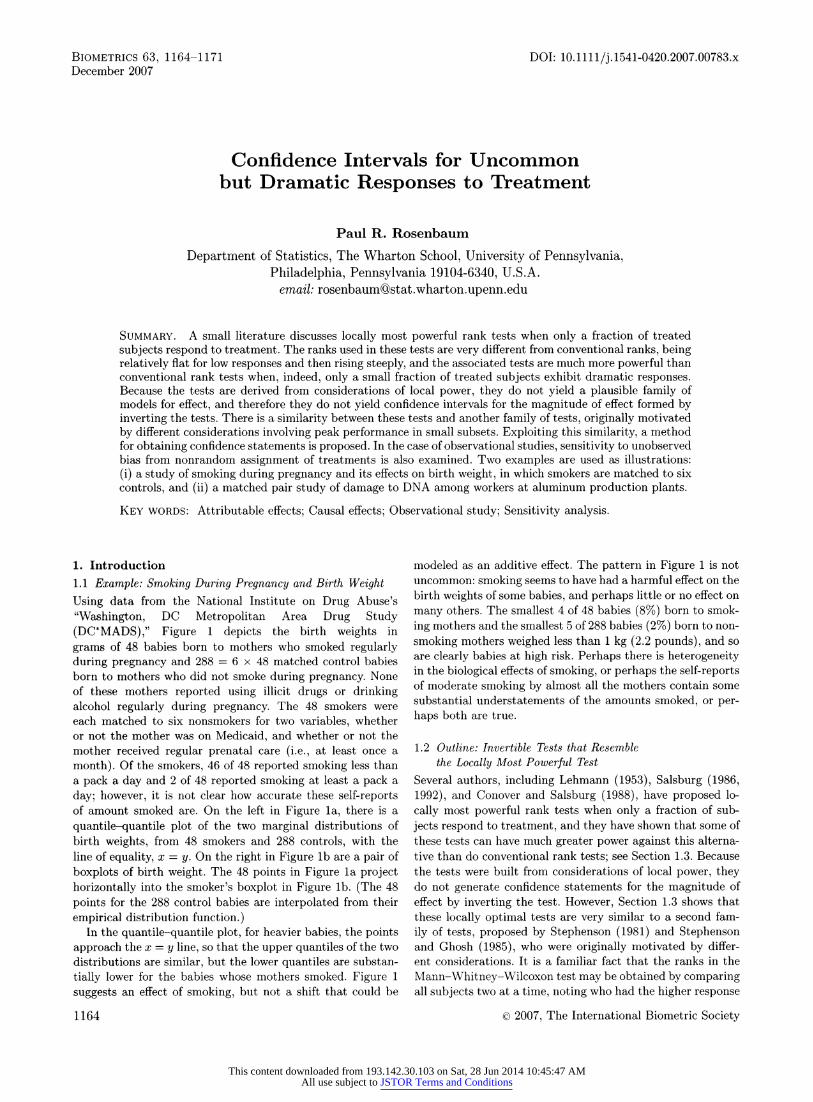
quantile-quantile plot of the two marginal distributions of birth weights, from 48 smokers and 288 controls, with the line of equality, x = y. On the right in Figure lb are a pair of

boxplots of birth weight. The 48 points in Figure la project horizontally into the smoker's boxplot in Figure lb. (The 48

points for the 288 control babies are interpolated from their

empirical distribution function.) In the quantile-quantile plot, for heavier babies, the points

approach the x = y line, so that the upper quantiles of the two distributions are similar, but the lower quantiles are substan-

tially lower for the babies whose mothers smoked. Figure 1 suggests an effect of smoking, but not a shift that could be

modeled as an additive effect. The pattern in Figure 1 is not uncommon: smoking seems to have had a harmful effect on the birth weights of some babies, and perhaps little or no effect on

many others. The smallest 4 of 48 babies (8%) born to smok-

ing mothers and the smallest 5 of 288 babies (2%) born to non-

smoking mothers weighed less than 1 kg (2.2 pounds), and so are clearly babies at high risk. Perhaps there is heterogeneity in the biological effects of smoking, or perhaps the self-reports of moderate smoking by almost all the mothers contain some substantial understatements of the amounts smoked, or perhaps both are true.

1.2 Outline: Invertible Tests that Resemble the Locally Most Powerful Test

Several authors, including Lehmann (1953), Salsburg (1986, 1992), and Conover and Salsburg (1988), have proposed lo-

cally most powerful rank tests when only a fraction of sub-

jects respond to treatment, and they have shown that some of these tests can have much greater power against this alternative than do conventional rank tests; see Section 1.3. Because the tests were built from considerations of local power, they do not generate confidence statements for the magnitude of effect by inverting the test. However, Section 1.3 shows that these locally optimal tests are very similar to a second fam-

ily of tests, proposed by Stephenson (1981) and Stephenson and Ghosh (1985), who were originally motivated by different considerations. It is a familiar fact that the ranks in the

Mann-Whitney-Wilcoxon test may be obtained by comparing all subjects two at a time, noting who had the higher response

1164 © 2007, The International Biometric



Confidence Intervals for Uncommon but Dramatic Responses to Treatment 1165

Figure la: Q-Q Plot Figure ib: Birthweight

0

- o E I ,

§-

§

0

00 0 o

So

0

o -o

I I I I I I

1000 2000 3000 4000 Smokers Controls Control

Figure 1. Birth weight of 48 babies born to mothers who smoked regularly during pregnancy and 288 = 6 x 48 matched control babies.

in each set of two subjects. Stephenson (1981) and Stephen- son and Ghosh (1985) suggested comparing subjects not two at a time but m at a time, for fixed m > 2, and this yields ranks very similar to those proposed by Conover and Sals- burg (1988). Notation is defined in Section 2.1, and a Web- based supplementary appendix Section 5 confirms that this second family of tests also has good power against alternatives in which only a fraction of subjects respond to treatment. The new confidence intervals are introduced in Section 2.2, with some suggestions for scaling to aid interpretation in Sec- tion 2.3. The example in Section 1.1 is examined again in Section 2.4. Section 2 concerns procedures that compete with the stratified Wilcoxon rank sum test, whereas in Section 3, attention shifts to paired data and competitors of Wilcoxon's signed rank test. A second, paired example is discussed in Section 3.2. A brief summary is provided in Section 4.

1.3 Review: Rank Tests Using Polynomial Functions of Ranks

When J sorted responses have ranks j = 1, 2,..., J, several investigators with varied motivations have proposed using rank scores that are polynomial functions of j, including, for fixed m, the functions jm-1, {J!(j + m- 2)!}/ {(J + m - 1)!(j - 1)!}, and

((-1l), each of which is a polyno-

mial in j of the order jm-1. Some investigators have been concerned with improved local power against constant treatment effects or shift alternatives, where fairly small increases in power were sometimes possible, but other investigators have been concerned with situations, such as Section 1.1, in which only a small fraction of treated subjects respond to treatment, where substantial increases in power are typical. None of these investigators proposed confidence intervals for the case of rare but dramatic responses to treatment, in part be-

cause their tests were built to be optimal against local alternatives, whereas a confidence interval is not a local statement. It turns out that these several tests behave similarly, and in later sections it is seen that one of the tests inverts grace- fully to yield exact or approximate confidence intervals for measures of rare but dramatic responses to treatment.

In unmatched comparisons of a total of J independent ob- servations divided between treated and control groups, with responses that have continuous distributions G(.) and F(.), respectively, one usually thinks of Wilcoxon's rank sum test as well designed to detect a constant effect or shift alternative, G(y) = F(y - 7), and indeed it is the locally most powerful rank test against a shift alternative when F(y) =

1/(1 + e-Y) is the logistic distribution. What if there is not a constant effect, the same for everyone, but rather only a small fraction of subjects, p, with 0 < p < 1, respond to the treatment? Perhaps surprisingly, Lehmann (1953, Section

6) showed that Wilcoxon's rank sum test is also the locally most powerful rank test against the alternative G(y) = (1 -

p)F(y) + pF2(y) as p - O0. In this alternative, 1 - p of the treated subjects are unaffected by treatment with the same distribution F(.) as controls, but a tiny fraction p are af- fected, with a stochastically larger distribution F2(.). After offering several biological mechanisms that might limit effects to a subset of treated subjects, Salsburg (1986) suggested the model G(y) = (1 - p)F(y) + pFm(y) where m > 1 need not be 2, and he suggested that the jth largest response might be assigned a rank proportional to jm-1, which of course yields conventional ranks when m = 2. Extending Lehmann's ar-

gument, Conover and Salsburg (1988) found the locally most

powerful test against G(y) = (1 - p)F(y) + pFm(y) as p 0 to assign the jth largest response the rank

SJ!(j + m - 2)! Pmj = (J + m- 1)!(j - 1)!

= (J+m-1)! (j + m - 2)(j + m - 3) ... (j),

which is a polynomial in j whose highest power of j is jm-1, so for large J, Salsburg's (1986) ranks jm-l and Conover and Salsburg (1988)'s ranks Pmj behave similarly. Conover and Salsburg (1988) argued that m = 5 is often a good choice when only a small fraction of treated subjects respond strongly.

Motivated by different considerations to be discussed later, Stephenson (1981) and Stephenson and Ghosh (1985) re- placed conventional ranks j = 1,. , J by ranks

gmj = (-), which are defined to be zero for j < m. A little arithmetic shows that these ranks are related to the Conover-Salsburg (1988) ranks by

mj (J+m-1) (j-1)(j-2)...(j-m+1) Pmj

J " j(j + 1) -" · (j

+ m -

for

j_

m, and mj =0 for j<m, Pm,

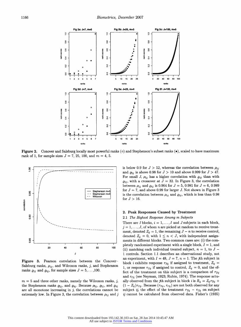
so that, as j and J increase, the ratio of these ranks tends to a constant. Figure 2 plots Pmj/PmJ and

Qmji/mJ against j, j =

1,...,J, for J = 7, 25, 100 and m = 4, 5. For J = 5,...,100, Figure 3 depicts the Pearson correla-

tion between the Conover and Salsburg (1988) ranks Psi

with



1166 Biometrics, December 2007

Fig 2a: J=7, m=5 Fig 2b: J=25, m=5 Fig 2c: J=100, m=5

o o6

U 1 C o4 5 05 0 5 0 20 Co

o 0

0 o

o Io o

1 2 3 4 5 6 7 5 10 15 20 25 0 20 40 60 80 100

ranks ranks ranks

Fig 2d: J=7, m=4 Fig 2e: J=25, m=4 Fig 2f: J=100, m=4 o o

,, Co Co

C 0 (

So0

0 c o0 o6 0 26

0§ 0

12 3 4 5 6 7 5 10 15 20 25 0 20 40 60 80 100

ranks ranks ranks

Figure 2. Conover and Salsburg locally most powerful ranks (o) and Stephenson's subset ranks (o), scaled to have maximum rank of 1, for sample sizes J = 7, 25, 100, and m = 4, 5.

- - - - - - - - - - - - - ---- - - - - -

O- Stephenson m=5

. Stephenson m=4 -- Wilcoxon

- • 0)

I I I I

20 40 60 80 100

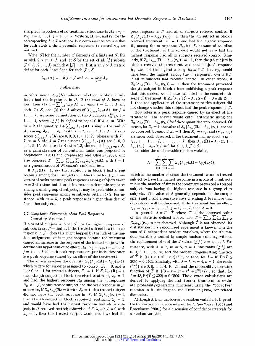
Figure 3. Pearson correlation between the Conover-

Salsburg ranks, P5j, and Wilcoxon ranks, j, and Stephenson ranks 5sj and 04j, for sample sizes J = 5,... ,100.

m = 5 and three other ranks, namely the Wilcoxon ranks, j, the Stephenson ranks Q5j, and Q4j. Because P5j, e5j, and Q4j are all monotone increasing in j, the correlations cannot be

extremely low. In Figure 3, the correlation between P5j and j

is below 0.9 for J > 12, whereas the correlation between psi and 05j is above 0.98 for J > 10 and above 0.999 for J > 47. For small J, P5j has a higher correlation with Q4j than with

s5j, with a crossover at J = 32. In Figure 3, the correlation

between P5j and 04j is 0.964 for J = 5, 0.981 for J = 6, 0.989 for J = 7, and above 0.99 for larger J. Not shown in Figure 3 is the correlation between P5j and sj , which is less than 0.98 for J> 16.

2. Peak Responses Caused by Treatment

2.1 The Highest Response Among m Subjects There are I blocks, i = 1,...,I and J subjects in each block, j = 1,..., J, of whom n are picked at random to receive treat-

ment, denoted Zij = 1, the remaining J - n to receive control, denoted Zij = 0, with 1 < n < J, with independent assign- ments in different blocks. Two common cases are: (i) the com-

pletely randomized experiment with a single block, I = 1, and

(ii) matching each individual treated subject, n = 1, to J - 1 controls. Section 1.1 describes an observational study, not an experiment, with I = 48, J = 7, n = 1. The jth subject in block i exhibits response rTij if assigned to treatment, Zj =

1, or response rcij if assigned to control, Zij = 0, and the effect of the treatment on this subject is a comparison of rTij and rcij (see Neyman, 1923; Rubin, 1974). The response actu-

ally observed from the jth subject in block i is R~j =

Zj rTij + (1 - Zij)rcij. Because (rTij, rcij) are not both observed for any subject ij, the effect of the treatment rTij - rcij on subject ij cannot be calculated from observed data. Fisher's (1935)




sharp null hypothesis of no treatment effect asserts Ho: rTij =

rcij, i = 1,..., I, j = 1,..., J. Write Z, R, rT, and rc for the corresponding I x J matrices. It is convenient to assume that for each block i, the J potential responses to control rcij are not tied.

Write IJI for the number of elements of a finite set J. Fix m with 2 < m < J, and let S be the set of all (J) subsets J E {1, 2,..., J} such that IJI = m. If A is an I x J matrix, define for each i and j and for each J E S

Aij(A)= 1 if j E and A = maxAik kEJ

= 0 otherwise;

in other words, A,5j(A) indicates whether in block i, subject j had the highest A in J. If the rows of A have no ties, then (1) 1= J A,jj(A) for each i= 1,...,I and each J E S, and (2) the J values of ZJES Aijj(A), for j -

1, ... , J, are some permutation of the J numbers (k-1), k =

1, .. , J, where (k-) is defined to equal 0 if k < m. With

m = 2, the quantity 1 + EJEs Aijj(A) is simply the rank of

Aj among Ail,..., A. With J = 7, m = 4, the J = 7 rank scores E ••s ijj(A) are 0, 0, 0, 1, 4, 10, 20, whereas with J =

7, m = 5, the J = 7 rank scores J-es ,ijj(A) are 0, 0, 0, 0, 1, 5, 15. As noted in Section 1.3, the use of ECJs Aijj(A) as a generalization of conventional ranks was proposed by Stephenson (1981) and Stephenson and Ghosh (1985), who also proposed T =

Ei=l Ej s ZA,(R), with I = 1, as a generalization of Wilcoxon's rank sum test.

If Aijj(R) = 1, say that subject j in block i had a peak response among the m subjects k in block i with k E J. Con- ventional ranks measure peak responses among subjects taken m = 2 at a time, but if one is interested in dramatic responses among a small group of subjects, it may be preferable to consider peak responses among m subjects with m > 2. For instance, with m = 5, a peak response is higher than that of four other subjects.

2.2 Confidence Statements about Peak Responses Caused by Treatment

If a treated subject in a set J has the highest response of subjects in set J-that is, if the treated subject has the peak response in J-then this might happen by the luck of the random assignment, or it might happen because the treatment caused an increase in the response of the treated subject. Un- der the null hypothesis of no effect; Ho : rT?, = rcij, i = 1, ..., I, j = 1,..., J, all such peak responses are just luck. How often is a peak response caused by an effect of the treatment?

The answer involves the quantity Zij{A,,•(R) - X, j(rc)},

which is zero for subjects assigned to control, Zi, = 0, and is 1 or 0 or -1 for treated subjects,

Zij = 1. If

ZiAj(R) = 1,

then the jth subject in block i received treatment, Z, = 1, and had the highest response R,0 among the m responses Rik, k E J, so this treated subject had the peak response in J; otherwise, if ZA,,j(R) = 0 with Z, = 1, this treated subject did not have the peak response in 3. If Z,Aij (rc)= 1, then the jth subject in block i received treatment, Zj = 1, and would have had the highest response had all m subjects in 3 received control; otherwise, if

ZijAj(rc) = 0 with

Zj = 1, then this treated subject would not have had the

peak response in J had all m subjects received control. If

Z,i{Aijj(R) - Aijs(rc)} = 1, then the jth subject in block i received treatment, Zij = 1, and had the highest response R, among the m responses Rik, k E J, because of an effect of the treatment, as this subject would not have had the highest response had all m subjects received control. Simi- larly, if Zij{A,ijj(R) - AXijj(rc)} = -1, then the jth subject in block i received the treatment, and that subject's response R, was not the highest among Rik, k E 3, but rci would have been the highest among the m responses, rcik, k E 3 if all m subjects had received control. In other words, if

Zij{•ijj(R) - Aijj(rc)} = -1 then the treatment prevented

the jth subject in block i from exhibiting a peak response that this subject would have exhibited in the complete ab- sence of treatment. If Zf{Aij(R) - Aij(rc)} = 0 with Zi =

1, then the application of the treatment to this subject did not change whether this subject had the peak response in J.

How often is a peak response caused by an effect of the treatment? The answer would entail arithmetic using the

Z, I{ij{j (R) - A,ijj(rc)}'s if these quantities were observed. Of

course, for Zj = 1, the value of Z, {ij ,ij(R) - A,ijj(rc)} cannot be observed, because if Zij = 1 then Rj = rTij, and (rTij, rcij) are never both observed. If the treatment had no effect, rTjj =

rc, i = 1, ...,I, j = 1, ...,J, then A3ij(R) - Ajj(rc) =

Aijj(rc) - Ajj(rc) = 0 for all i, j, J E S. Consider the unobservable random variable,

I J

A = E Zij{Aij,(R) -

Aj(rc)}, i=1 j=1 JES

which is the number of times the treatment caused a treated subject to have the highest response in a group of m subjects minus the number of times the treatment prevented a treated subject from having the highest response in a group of m subjects. The value of A generally depends on the sample size, I and J, and alternative ways of scaling A to remove that dependence will be discussed. If the treatment has no effect, rTij =

rco,, i = 1,..., I, j = 1,..., J, then A = 0.

In general, A = T - T where T is the observed value of the statistic defined above, and T= =1 =1 •JS ZAijj(rc) is not observed. Although T is not observed, its distribution in a randomized experiment is known: it is the sum of I independent random variables, where the ith random variable is formed by simple random sampling without the replacement of n of the J values (k-), 1,... , J. For

instance, with J = 7, m = 5, n = 1, the ranks (mk-1) are 0, 0, 0, 0, 1, 5, 15, and the probability-generating function of T is {(4 + x+ x + x 15)/7}I, so that, for I= 48,Pr(T 205) = 0.9501. Similarly, with J = 7, m = 4, n = 1, the ranks

(m-j) are 0, 0, 0, 1, 4, 10, 20, and the probability-generating function of T is {(3 + x + x4 + X10 + X20)/7}I, SO that, for I = 48, Pr(T 322) = 0.9506. These exact calculations derived by applying the fast Fourier transform to evalu- ate probability-generating functions, using the "convolve" function in R; see Pagano and Tritchler (1983) for related discussion.

Although A is an unobservable random variable, it is possible to create a confidence interval for A. See Weiss (1955) and Rosenbaum (2001) for a discussion of confidence intervals for a random variable.




PROPOSITION 1. In a randomized experiment, if Pr(T < f) = 1 - a, then with 100(1 - a)% confidence, A > T - e.

Proof. From A = T - T, it follows that 1 - a = Pr{T <

f} = Pr{T - A <£} = Pr{A

> T

-

As noted above, the probability Pr{T < £} needed

Proposition 1 may be obtained exactly using probability- generating functions. Alternatively, an approximation may be based on the central limit theorem, Pr{(T - p)/a > v} -

1 - '(v) as I -* oo, where p = E(T) and a2 = var(T) are

p = nIq, 2

_nI(J-n),

where J(J -

1)J

qj = (m andq

J q (1)

j=1

With I = 48, J = 7, n = 1, m = 5, one has p = 144, a2

1289.143, so the exact Pr(T < 205) = 0.9501 is approximated by (I{(205 - 144)/v1}289.143} = 0.955.

2.3 Scaling A to Aid Interpretation The unobservable quantity A = T - T counts the increase in

peak performance by treated subjects caused by the effects of the treatment, and because it is a count, it generally depends upon the sample size, I and J. It aids in interpretation to divide A by a known constant, so that the magnitude of the scaled version has a meaning that is not linked to the sample size. Two possible divisors are considered.

With the constant E(T) = p = nIq defined in (1), the

quantity A/p is the multiplicative increase above chance ex-

pectation in the number of times treated subjects had a peak performance in subsets of m subjects because of the effects caused by the treatment. If the treatment has no effect, then A = 0, so A/p = 0 also. From Proposition 1, with 95% confi-

dence, A/p >_

(T - £)/p. Also, (T - p)/p is a consistent estimate of A/p = (T - T)/p in the sense that the difference between these two random variables converges in probability to 0 as I -- 00o.

An alternative divisor creates a correlation-like measure scaled to be 0 for a chance agreement and 1 for perfect agreement. The maximum possible value of T is tma,, =

S- ·j=J_ (_n+1( ).

The quantity A/(tmax - p) = (T -

(tmax - p) takes the value 0 under the null hypothesis of no treatment effect, and it has expectation 1 if the treatment

always raises the responses of all treated subjects above the responses of all controls in the same matched set. From Propo- sition 1, with 95% confidence, A/(tmax - p) (T - (tmax - p), and (T - p)/(tma,, - p) is a consistent point estimate of A/(tmax - /) = (T - T)/(tmax - t) as I - 00o.

2.4 Example, Continued: Smoking During Pregnancy and Birth Weight

In Section 1.1, the concern is with the smallest babies, so "peak" refers to smallest rather than largest in a group of m babies. Recall that there were I = 48 matched sets consisting of n = 1 baby whose mother smoked during pregnancy and J - n = 6 babies whose mothers did not smoke during pregnancy. The current section will analyze the data in Section 1.1 as if one mother had been picked at random to smoke in each

matched set of J = 7. Nonrandom treatment assignment is discussed in Section 2.5.

Consider, first, m = 5, along the lines suggested by Sals-

burg (1986) and Conover and Salsburg (1988). In a matched set of J = 7 babies, there are (j-1)) = ( ) = 15 subsets con-

sisting of the n = 1 baby whose mother smoked during pregnancy and four other babies. If the one exposed baby had the smallest birth weight of all seven babies, then that baby is smallest in all 15 subsets and receives a rank score of 15, but if the exposed baby had the second smallest birth weight, then that baby is smallest in the (7-2) = 5 of the 15 subsets that exclude the smallest baby, so the rank is 5, etc., for possible ranks 15, 5, 1, 0, 0, 0, 0. If smoking had no effect on birth weight and smoking behavior had been ran-

domly assigned to one mother in each matched set, then by chance alone, we expect the exposed baby to be the smallest in 3 = (15 + 5 + 1 + 0 + 0 + 0 + 0)/7 of the 15 subsets. For the I = 48 matched sets together, by chance alone we expect the baby whose mother smoked to be the smallest in t = nIq = 48 x 3= 144 of the tmax = I J n+ -1)

4j=J-n+lm-1 48(J-1) = 48 x 15 = 720 subsets of m = 5 babies. In fact, the

baby whose mother smoked was the smallest not in p = 144 sets of m = 5 babies, but in T = 264 sets of m = 5 babies. As calculated in Section 2.3, Pr(T < 205) = 0.9501, so from

Proposition 1, we are 95% confident that in at least A > T - £ = 264 - 205 = 59 of these subsets, smoking caused the

posed baby to have the smallest birth weight of m = 5 babies. The point estimate, (T - I)/p = (264 - 144)/144 = 0.83, suggests that smoking caused an increase of 83% in the number of peakedly small babies over what was expected by chance, but we are 95% confident of only an increase of (264 -

205)/144 = 59/144 = 0.41 or 41%. Consider subsets of size m = 2 rather than m = 5. As in

Section 2.1, the ranks for m = 2 are one less than Wilcoxon's

ranks, yielding the same significance levels and power. The stratified Wilcoxon statistic is T + I = 186 + 48 = 234, where T = 186, p = nIq = 48 x (0 + 1 +-- + 6)/7 = 144, so that the exposed baby was the smaller baby in 186 pairwise comparisons of two babies, with 144 expected by chance. As 0.9551 = Pr(T < 167), we are 95% confident that at least A > T - £ = 186 - 167 = 19 of the 186 comparisons were

by smoking. The point estimate is an increase of (T - p)/p =

(186 - 144)/144 = 0.29 or 29% above chance, but we are 95% confident of only an increase of (186 - 167)/144 = 19/144 = 0.13 or 13%.

2.5 Sensitivity Analysis for Nonrandom Treatment Assignment

The analysis in Section 2.4 viewed smoking during pregnancy as a treatment that was randomly assigned to one mother in each matched set, but of course this is not true. A sensitivity analysis in an observational study asks how the conclusions might be altered by departures from random assignment of various magnitudes. The first such sensitivity analysis was performed by Cornfield et al. (1959), and it concerned the association between heavy smoking and lung cancer. Cornfield et al. showed that to explain away that association as not caused by smoking, and instead created by failure to match on an unobserved covariate u, one would have to postulate an enormous departure from random assignment, as measured by a parameter describing the relationship between treatment




assignment and u. A related but slightly more general approach assumes that two subjects with the same observed covariates might differ in their odds of treatment by at most a factor of F > 1 because of the failure to also match for an unobserved covariate u, and then for several values of F calculates the range of possible values of inference quantities, such as significance levels, point estimates, or confidence intervals (see Rosenbaum, 1987, 2002, Section 4). Because T is simply a linear rank statistic with somewhat unusual rank scores, existing methods of sensitivity analysis for linear rank statistics apply immediately. For matching with multiple controls, the large sample procedure is described in Gastwirth, Krieger, and Rosenbaum (2000) or Rosenbaum (2002, Sec- tion 4.5), where all technical details may be found. Here, the large sample sensitivity analysis will be briefly illustrated for inference about A in Section 2.4 for smoking and birth weight. Other methods of sensitivity analysis are discussed by Lin, Psaty, and Kronmal (1998); Robins, Rotnitzky, and Scharfstein (1999); Copas and Eguchi (2001); and Imbens

(2003). For F = 1, one obtains the randomization inference, as de-

scribed in Section 2.4, with m = 5, where the null hypothesis of no effect is rejected with an approximate one-sided significance level of 0.00035. If F were 1.5, if the odds ratio linking smoking with an unobserved binary covariate were 1.5, then two mothers matched for observed covariates might differ by a factor of 1.5 in their odds of smoking. For F = 1.5, m =

5, the maximum possible significance level is 0.021, whereas at about F = 5/3, the maximum possible significance level is 0.045 and so is close to crossing the conventional 0.05 level. If the stratified Wilcoxon test with m = 2 is used in place of Stephenson's ranks with m = 5, then for F = 1, 1.5, and 5/3, the upper bounds on the significance level are, respectively, 0.0012, 0.035, and 0.066; therefore, in this one example, there is slightly less sensitivity to bias from unobserved covariates using m = 5 than using m = 2.

With I = 48, J = 7, n = 1, m = 5, as in Section 2.4, and with F = 1.5, the largest upper tail probabilities for T come from an approximate normal distribution with expectation 186 and variance 1535.25, using the method in Gastwirth et al. (2000, Section 3.1) or Rosenbaum (2002, Section 4.5.2), so this approximation yields Pr(T > f) <

0.05 with f - 186 + 1.65v/1535.25 = 250.65 " 251, where 0.05 1 - 4Q(1.65), and 4(.) is the standard normal cumulative distribution. In parallel with Proposition 1, if F were 1.5, with at least 95% confidence, A > T -

£ = 264 - 251 = 13

than A > 59 for F = 1 in Section 2.4, so a bias of magnitude F = 1.5 could explain some of the extremely low birth weights of babies born to smokers, but not all of them. At F = 5/3, the continuous normal approximation only permits one to say with 95% confidence that A is greater than zero. The comparison in Figure 1 is insensitive to small biases, but could be produced by a moderate bias of F = 2, so it is much more sensitive to unobserved bias than, say, Hammond's (1964) study of smoking as a cause of lung cancer, which is insensitive to a very large bias of F = 5 (see Rosenbaum, 2002, Table 4.1). Moderate biases are not inconceivable in Figure 1, because a mother who smokes during pregnancy may also be less cau- tious in the use of other substances, such as alcohol, medica- tions, or narcotics.

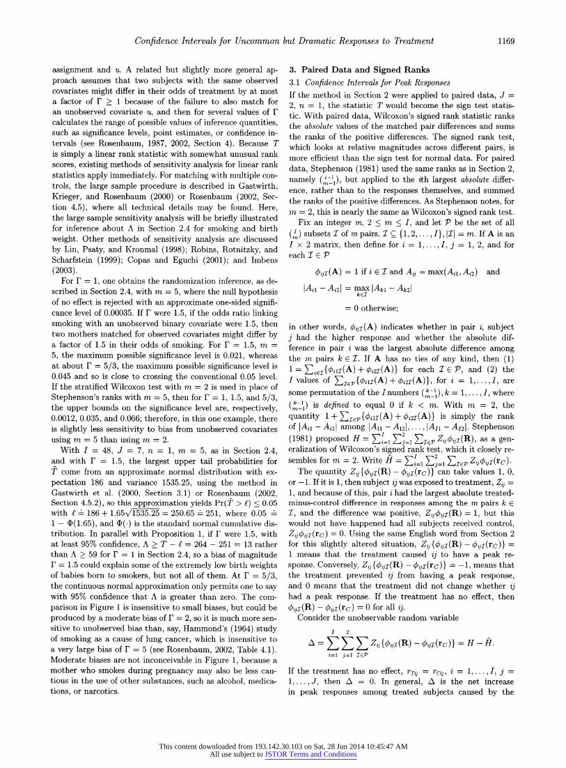
3. Paired Data and Signed Ranks

3.1 Confidence Intervals for Peak Responses If the method in Section 2 were applied to paired data, J = 2, n = 1, the statistic T would become the sign test statistic. With paired data, Wilcoxon's signed rank statistic ranks the absolute values of the matched pair differences and sums the ranks of the positive differences. The signed rank test, which looks at relative magnitudes across different pairs, is more efficient than the sign test for normal data. For paired data, Stephenson (1981) used the same ranks as in Section 2, namely

(i-1l), but applied to the ith largest absolute differ-

ence, rather than to the responses themselves, and summed the ranks of the positive differences. As Stephenson notes, for m = 2, this is nearly the same as Wilcoxon's signed rank test.

Fix an integer m, 2 < m < I, and let P be the set of all

(4) subsets I of m pairs, I C {1, 2,..., I}, I11 = m. If A is an I x 2 matrix, then define for i = 1,..., I, j = 1, 2, and for each I E P

$ijz(A) = 1 if i E Z and A0

= max(Ail, Ai2) and

|Aii - Ai21 = max IAkl - Ak21 kEI

= 0 otherwise;

in other words, zij1(A) indicates whether in pair i, subject j had the higher response and whether the absolute difference in pair i was the largest absolute difference among the m pairs k E 1. If A has no ties of any kind, then (1) 1 = iEz{oilz(A) + Oi2z(A)} for each I E P, and (2) the

I values of EZ.~.{iiZ(A)+ i2Z(A)}, for i = 1,... , I, are some permutation of the I numbers (k-), k = 1,..., I, where

(m-l'

(k-l) is defined to equal 0 if k < m. With m = 2, the quantity 1 + eEE{qilz(A) + qi2i(A)} is simply the rank of IAil - Ai21 among IAll - A12 I,..., IA1 - A12 I. Stephenson (1981) proposed H =

I=l =E 1 2= ZZOz(R), as a gen-

eralization of Wilcoxon's signed rank test, which it closely re- sembles for m = 2. Write H = =1~ ~i Z, (rc)

The quantity Zij{@qjz(R) - ijz(rc)} can take values 1, 0, or -1. If it is 1, then subject ij was exposed to treatment, Zij = 1, and because of this, pair i had the largest absolute treated- minus-control difference in responses among the m pairs k E I, and the difference was positive, Zijijz(R) = 1, but this would not have happened had all subjects received control, Zijijz(rc) = 0. Using the same English word from Section 2 for this slightly altered situation, ZijJ{ijz(R) -

yz(rc)} =

1 means that the treatment caused ij to have a peak response. Conversely, Zj {$,jz(R) - bjz(rc)} = -1, means that the treatment prevented ij from having a peak response, and 0 means that the treatment did not change whether ij had a peak response. If the treatment has no effect, then

qij5(R) -

kij-(rc) = 0 for all ij.

Consider the unobservable random variable

I 2

A = Z

Z,{j(R)

- 4zi(rc)}

= H - H. i=1 j=l ZEP

If the treatment has no effect, rTr = rc0, i = 1,..., I, j = 1,...,J, then A = 0. In general, A is the net increase in peak responses among treated subjects caused by the




treatment. The proof of Proposition 2 parallels the proof of

Proposition 1.

PROPOSITION 2. In a randomized experiment, if Pr(H _< h) = 1 - a, then with 100(1 - a)% confidence, A > H - h.

In a randomized experiment without ties, writing

qi = ('-'1), with qj defined to be 0 for i < m, the probability generating function of

Ht is

2-'H~1{1 + xq }, the

expectation and variance of H are E(H) = (1/2) II=, qj and

var(Hi) = (1/4) Z =1 q., so by the central limit theorem, as I - oc, Pr(H < h) may be approximated by )[(h - E(H)}/

/var(H)]. In parallel with Section 2.5, the large sample sensitivity bounds in Rosenbaum (1987) for Pr(H < h) are

I[(h - (}/f/]

and I[(h - J}/IVI] where 1 = (1/(1 + F)} x

qji,(= {r/(1 + r)} i qj, and v= {/(1 + )2

i= q, which reduce to standard formulas when F = 1.

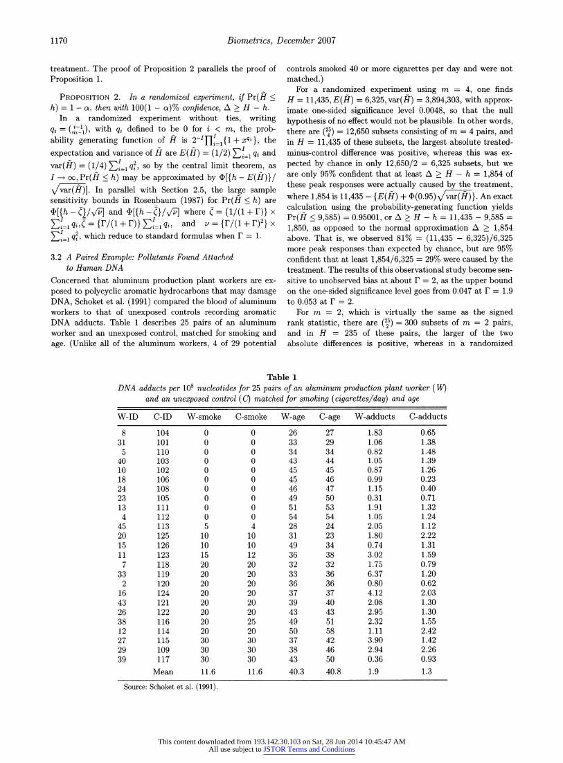
3.2 A Paired Example: Pollutants Found Attached to Human DNA

Concerned that aluminum production plant workers are ex-

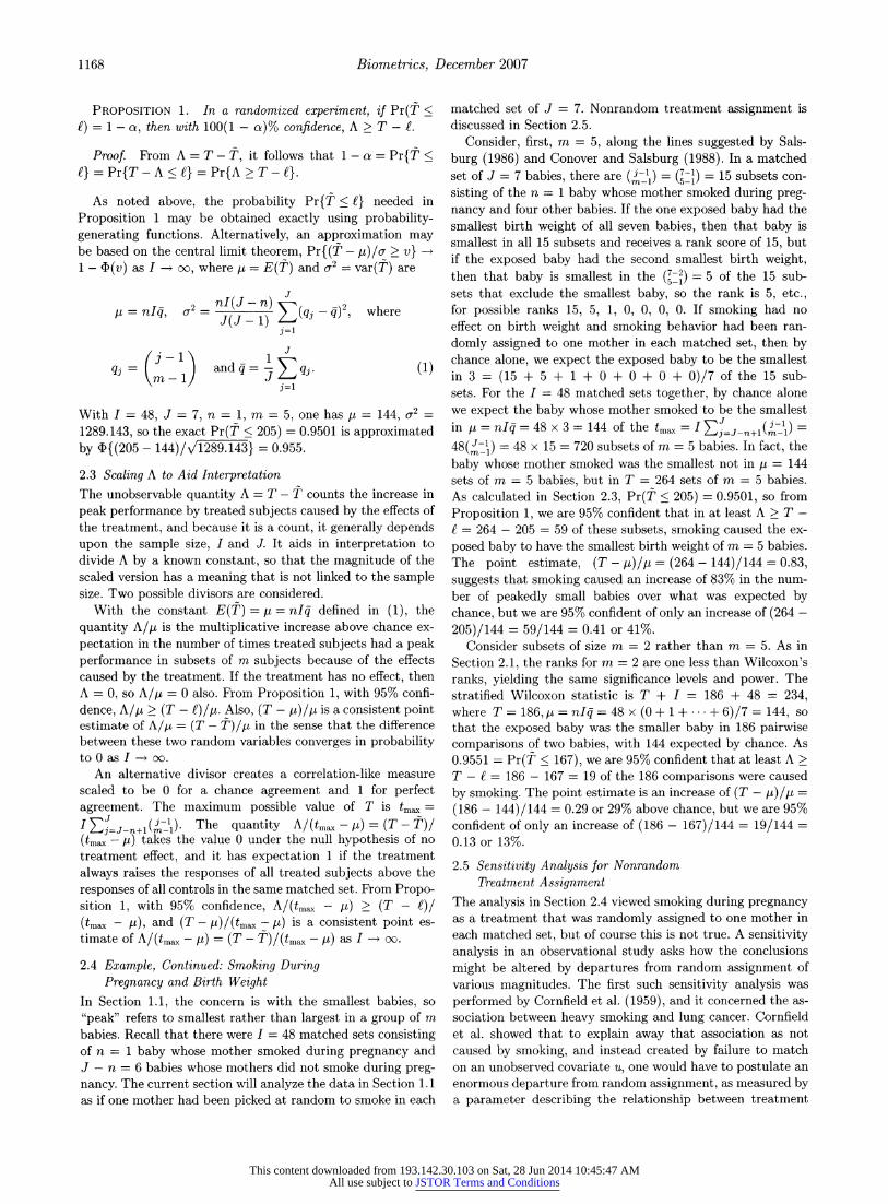
posed to polycyclic aromatic hydrocarbons that may damage DNA, Schoket et al. (1991) compared the blood of aluminum workers to that of unexposed controls recording aromatic DNA adducts. Table 1 describes 25 pairs of an aluminum worker and an unexposed control, matched for smoking and

age. (Unlike all of the aluminum workers, 4 of 29 potential

controls smoked 40 or more cigarettes per day and were not

matched.) For a randomized experiment using m = 4, one finds

H = 11,435, E(H) = 6,325, var(H) = 3,894,303, with approximate one-sided significance level 0.0048, so that the null

hypothesis of no effect would not be plausible. In other words, there are (25) = 12,650 subsets consisting of m = 4 pairs, and in H = 11,435 of these subsets, the largest absolute treated- minus-control difference was positive, whereas this was ex-

pected by chance in only 12,650/2 = 6,325 subsets, but we are only 95% confident that at least A > H - h = 1,854 of these peak responses were actually caused by the treatment, where 1,854 is 11,435 - {E(H) + 4(0.95) vvar()}. An exact calculation using the probability-generating function yields Pr(H < 9,585) = 0.95001, or A > H - h = 11,435 - 9,585 =

1,850, as opposed to the normal approximation A > 1,854 above. That is, we observed 81% = (11,435 - 6,325)/6,325 more peak responses than expected by chance, but are 95% confident that at least 1,854/6,325 = 29% were caused by the treatment. The results of this observational study become sensitive to unobserved bias at about F = 2, as the upper bound on the one-sided significance level goes from 0.047 at F = 1.9 to 0.053 at F = 2.

For m = 2, which is virtually the same as the signed rank statistic, there are (1) = 300 subsets of m = 2 pairs, and in H = 235 of these pairs, the larger of the two absolute differences is positive, whereas in a randomized

Table 1 DNA adducts per 10s nucleotides for 25 pairs of an aluminum production plant worker (W)

and an unexposed control (C) matched for smoking (cigarettes/day) and age

W-ID C-ID W-smoke C-smoke W-age C-age W-adducts C-adducts

8 104 0 0 26 27 1.83 0.65 31 101 0 0 33 29 1.06 1.38

5 110 0 0 34 34 0.82 1.48 40 103 0 0 43 44 1.05 1.39 10 102 0 0 45 45 0.87 1.26 18 106 0 0 45 46 0.99 0.23 24 108 0 0 46 47 1.15 0.40 23 105 0 0 49 50 0.31 0.71 13 111 0 0 51 53 1.91 1.32 4 112 0 0 54 54 1.05 1.24

45 113 5 4 28 24 2.05 1.12 20 125 10 10 31 23 1.80 2.22 15 126 10 10 49 34 0.74 1.31 11 123 15 12 36 38 3.02 1.59 7 118 20 20 32 32 1.75 0.79

33 119 20 20 33 36 6.37 1.20 2 120 20 20 36 36 0.80 0.62

16 124 20 20 37 37 4.12 2.03 43 121 20 20 39 40 2.08 1.30 26 122 20 20 43 43 2.95 1.30 38 116 20 25 49 51 2.32 1.55 12 114 20 20 50 58 1.11 2.42 27 115 30 30 37 42 3.90 1.42 29 109 30 30 38 46 2.94 2.26 39 117 30 30 43 50 0.36 0.93

Mean 11.6 11.6 40.3 40.8 1.9 1.3

Source: Schoket et al. (1991).




experiment, E(H) = 150 were expected by chance, with one- sided significance level 0.008. This is (235 - 150)/150 = 57% more than expected by chance, but we are 95% confident that at least A > H - h = 235 - {150 + 1.65v/1,225} = 27 or

27/150 = 18% were peak responses caused by the treatment. With m = 2, the results of this observational study become sensitive to unobserved bias at about F = 1.5, as the one- sided significance level goes from 0.041 at F = 1.4 to 0.054 at F = 1.5.

4. Summary Conover and Salsburg (1988) developed a locally most powerful rank test when only a subset of treated subjects respond strongly to treatment. Motivated by different considerations, Stephenson (1981) and Stephenson and Ghosh (1985) proposed rank tests focused on peak performance in small subsets. It was noted that these two different ranks are similar, and that Stephenson's tests can be inverted to provide confidence intervals for the number of peak performances actually caused by exposure to the treatment. Sensitivity analysis in observational studies was also discussed.

In both examples, dramatic responses were more common among treated subjects. When compared to conventional rank tests, rank tests designed with this alternative in mind yielded: (i) smaller significance levels from the randomization distribution, (ii) higher point estimates and confidence intervals formed by inverting these tests, and (iii) less sensitivity to unobserved biases in observational studies.

5. Supplementary Materials

A web-based appendix referenced in Section 1.2 is available under the Paper Information line at the Biometrics website, http://www.tibs.org/biometrics.

ACKNOWLEDGEMENT

This study was supported by a grant from the U.S. National Science Foundation.

REFERENCES

Conover, W. J. and Salsburg, D. S. (1988). Locally most powerful tests for detecting treatment effects when only a subset of patients can be expected to 'respond' to treatment. Biometrics 44, 189-196.

Copas, J. and Eguchi, S. (2001). Local sensitivity approxima- tions for selectivity bias. Journal of the Royal Statistical Society B 63, 871-896.

Cornfield, J., Haenszel, W., Hammond, E., Lilienfeld, A., Shimkin, M., and Wynder, E. (1959). Smoking and lung cancer. Journal of the National Cancer Institute 22, 173- 203.

Fisher, R. A. (1935). The Design of Experiments. Edinburgh: Oliver & Boyd.

Gastwirth, J. L., Krieger, A. M., and Rosenbaum, P. R. (2000). Asymptotic separability in sensitivity analysis. Journal of the Royal Statistical Society B 62, 545-555.

Hammond, E. C. (1964). Smoking in relation to mortality and morbidity. Journal of the National Cancer Institute 32, 1161-1188.

Imbens, G. W. (2003). Sensitivity to exogeneity assumptions in program evaluation. American Economic Review 93, 126-132.

Lehmann, E. L. (1953). The power of rank tests. Annals of Mathematical Statistics 24, 23-43.

Lin, D. Y., Psaty, B. M., and Kronmal, R. A. (1998). As- sessing the sensitivity of regression results to unmeasured confounders in observational studies. Biometrics 54, 948-963.

Neyman, J. (1923). On the application of probability theory to agricultural experiments. Reprinted in Statistical Science 1990, 5, 463-480.

Pagano, M. and Tritchler, D. (1983). On obtaining permutation distributions in polynomial time. Journal of the American Statistical Association 78, 435-440.

Robins, J. M., Rotnitzky, A., and Scharfstein, D. (1999). Sen- sitivity analysis unmeasured confounding in missing data and causal inferenc. In Statistical Models in Epidemiol- ogy, E. Halloran and D. Berry (eds), 1-94. New York: Springer.

Rosenbaum, P. R. (1987). Sensitivity analysis for certain permutation inferences in matched observational studies. Biometrika 74, 13-26.

Rosenbaum, P. R. (2001). Effects attributable to treatment: Inference in experiments and observational studies with a discrete pivot. Biometrika 88, 219-231.

Rosenbaum, P. R. (2002). Observational Studies. New York: Springer.

Rubin, D. B. (1974). Estimating causal effects of treatments in randomized and nonrandomized studies. Journal of Educational Psychology 66, 688-701.

Salsburg, D. S. (1986). Alternative hypotheses for the effects of drugs in small-scale clinical studies. Biometrics 42, 671-674.

Salsburg, D. S. (1992). The Use of Restricted Significance Tests in Clinical Trials. New York: Springer.

Schoket, B., Phillips, D. H., Hewer, A., and Vincze, I.

(1991). 32P-Postlabelling detection of aromatic DNA adducts in peripheral blood lymphocytes from aluminum production plant workers. Mutation Research 260, 89- 98.

Stephenson, W. R. (1981). A general class of one-sample non- parametric test statistics based on subsamples. Journal of the American Statistical Association 76, 960-966.

Stephenson, W. R. and Ghosh, M. (1985). Two sample non- parametric tests based on subsamples. Communications in Statistics 14, 1669-1684.

Weiss, L. (1955). A note on confidence sets for random variables. Annals of Mathematical Statistics 26, 142-144.

Received September 2006. Revised December 2006. Accepted December 2006.



Documents

Confidence Intervals for Uncommon but Dramatic Responses to Treatment