Confidence intervals for causal effects with invalid

© 2018 Royal Statistical Society 1369–7412/18/80793

J. R. Statist. Soc. B (2018)80, Part 4, pp. 793–815

Confidence intervals for causal effects with invalidinstruments by using two-stage hard thresholdingwith voting

Zijian Guo,

Rutgers University, Piscataway, USA

Hyunseung Kang

University of Wisconsin—Madison, Madison, USA

and T. Tony Cai and Dylan S. Small

University of Pennsylvania, Philadelphia, USA

[Received August 2016. Final revision March 2018]

Summary. A major challenge in instrumental variable (IV) analysis is to find instruments thatare valid, or have no direct effect on the outcome and are ignorable. Typically one is unsurewhether all of the putative IVs are in fact valid. We propose a general inference procedure inthe presence of invalid IVs, called two-stage hard thresholding with voting. The procedure usestwo hard thresholding steps to select strong instruments and to generate candidate sets ofvalid IVs. Voting takes the candidate sets and uses majority and plurality rules to determine thetrue set of valid IVs. In low dimensions with invalid instruments, our proposal correctly selectsvalid IVs, consistently estimates the causal effect, produces valid confidence intervals for thecausal effect and has oracle optimal width, even if the so-called 50% rule or the majority ruleis violated. In high dimensions, we establish nearly identical results without oracle optimality. Insimulations, our proposal outperforms traditional and recent methods in the invalid IV literature.We also apply our method to reanalyse the causal effect of education on earnings.

Keywords: Exclusion restriction; High dimensional covariates; Invalid instruments; Majorityvoting; Plurality voting; Treatment effect

1. Introduction

1.1. Motivation: invalid instrumentsInstrumental variable (IV) analysis is a popular method to deduce causal effects in the presenceof unmeasured confounding. Informally, an IV analysis requires instruments that

(a) are associated with the exposure (assumption 1),(b) have no direct pathway to the outcome (assumption 2) and(c) are not related to unmeasured variables that affect the exposure and the outcome (as-

sumption 3); see Section 2.1 for details.

A major challenge in IV analysis is to find valid instruments, i.e. instruments that satisfy as-sumptions 2 and 3.

Address for correspondence: Dylan S. Small, Department of Statistics, University of Pennsylvania, WhartonSchool, 400 Huntsman Hall, 3730 Walnut Street, Philadelphia, PA 19104, USA.E-mail: [email protected]

794 Z. Guo, H. Kang, T. T. Cai and D. S. Small

For example, a long-standing interest in economics is studying the causal effect of educationon earnings (Angrist and Krueger, 1991; Card, 1993, 1999). Often, IV analysis is used to deducethis effect and a popular instrument for the analysis is a person’s proximity to a college whengrowing up (Card, 1993, 1999). However, proximity to a college may be related to a person’ssocio-economic status, high school characteristics and other variables that may affect a person’searnings, thereby invalidating the instrument. Often, covariates, potentially many, are controlledfor to make instruments more plausibly valid (Hernan and Robins, 2006; Swanson and Hernan,2013; Baiocchi et al., 2014; Imbens, 2014). For instance, in the earnings example, socio-economicstatus, family background and genetic status can be controlled for to alleviate concerns aboutinstrument validity.

But, some IVs may still turn out to be invalid after controlling and subsequent analysisassuming that all the IVs are valid after conditioning can be misleading (Murray, 2006). Forinstance, in the earnings example with proximity as the instrument, if living close to college hadother benefits beyond receiving more education, say by being exposed to many programmesthat are available to high school students for job preparation and employers who come to thearea to discuss employment opportunities for college students, then the IV can directly affectan individual’s earning potential and violate assumption 2 (Card, 1999). This problem is alsoprevalent in other applications of IVs, most notably in Mendelian randomization (Davey Smithand Ebrahim, 2003, 2004) where the instruments are genetic in nature and some instrumentsare likely to be invalid because they have pleiotropic effects (Lawlor et al., 2008; Burgess et al.,2015).

This paper tackles the problem of constructing confidence intervals for causal effects wheninvalid instruments may be present. We consider two major cases. The first case is where thenumber of covariates and instruments is small and fixed relative to the sample size; this setting istypical in Mendelian randomization studies and many traditional applied settings. The secondcase is where the number of covariates and/or instruments is growing and may exceed the samplesize, which is becoming more prevalent with modern large data sets.

1.2. Prior work and our contributionsIn non-IV settings with high dimensional covariates as controls, Zhang and Zhang (2014),Javanmard and Montanari (2014), van de Geer et al. (2014), Belloni et al. (2014) and Cai andGuo (2017) have provided confidence intervals for a treatment effect. In IV settings with highdimensional covariates (or IVs), Gautier and Tsybakov (2011), Belloni et al. (2012), Fan andLiao (2014) and Chernozhukov et al. (2015) have provided confidence intervals for a treatmenteffect, under the assumption that all the IVs are valid after controlling for the said covariates.In invalid IV settings, Kolesar et al. (2015) and Bowden et al. (2015) have provided inferentialmethods for treatment effects. However, the method requires that the effects of the instrumentson the treatment are orthogonal to their direct effects on the outcome, which is a stringentassumption. Bowden et al. (2016), Burgess et al. (2016), Kang et al. (2016b) and Windmeijeret al. (2016) also worked on the invalid IV setting, but without making a stringent orthogonalityassumption.

Unfortunately, all of these methods

(a) work only in the low dimensional setting and(b) rely on the sufficient condition in Han (2008) and Kang et al. (2016b),

which is known as the ‘50% rule’ or the ‘majority rule’ where a majority of the instruments mustbe valid to establish consistency or inferential guarantees (see Section 2.2 for details); to the bestof our knowledge, no method in this literature has established consistency, inferential and oracle

Confidence Intervals by using Two-stage Hard Thresholding with Voting 795

guarantees under a general condition established in theorem 1 of Kang et al. (2016b), includingthe setting where the majority rule is violated; see Section 3.6 for a review and a comparison ofthe methods in the literature with our proposed method.

Our work makes three major contributions in inferring treatment effects in the presence ofpossibly invalid instruments. First, we propose a novel two-stage hard thresholding (TSHT)method with voting that works both in low and high dimensional settings. Second, in the lowdimensional setting, our method is the first method to be complete; our method relies only ona general condition for identification under invalid instruments to

(a) to select valid IVs correctly,(b) to estimate the causal effect consistently,(c) to produce confidence intervals with the desired level of coverage and(d) to achieve oracle optimality in the sense that it performs as well asymptotically as the

oracle procedure that knows which instruments are valid.

In particular, our method can guarantee these properties even when more than 50% of theinstruments are invalid as long as a more general condition, which we call the plurality rule,holds; see Section 2.2 for details. Third, in the high dimensional setting, our method achievesthe same selection, estimation and inferential guarantees without the oracle optimality.

The outline of the paper is as follows. After describing the model set-up in Section 2, wedescribe our procedure TSHT with voting in Section 3 and provide theoretical justification forit in Section 4. In Section 5, we investigate the performance of our procedure in a simulation studyand compare it with existing methods, in particular the median method with bootstrapping ofBowden et al. (2016) and Burgess et al. (2016) and the adaptive lasso method of Windmeijeret al. (2016). We find that our method and that of Windmeijer et al. (2016) are comparable whenthe 50% rule holds, whereas the median estimator suffers from coverage and optimality issues.However, when the 50% rule fails, our method dominates all these methods. In Section 6, wepresent an empirical study where we revisit the question of the causal effect of years of schoolingon income by using data from the Wisconsin longitudinal study (WLS). We provide conclusionsand discussions in Section 7. The code to implement the proposed method along with a runningexample is available from https://github.com/hyunseungkang/invalidIV.

2. Model

To define causal effects and instruments, the potential outcome approach (Neyman, 1923; Ru-bin, 1974) that is laid out in Holland (1988) is used. For each individual i ∈ {1, : : : , n}, letY

.d,z/i ∈ R be the potential outcome if the individual were to have exposure or treatment d ∈ R

and instruments z∈Rpz . Let D.z/i ∈R be the potential exposure if the individual had instruments

z∈Rpz . For each individual, only one possible realization of Y.d,z/i and D

.z/i is observed, denoted

as Yi and Di respectively, based on his or her observed candidate instrument values Zi: ∈ Rpz

and exposure value Di. We also denote baseline covariates for each individual i as Xi: ∈Rpx . Intotal, n sets of outcome, exposure, instruments and baseline covariates, which are denoted as.Yi, Di, Zi:, Xi:/, are observed in an independent and identically distributed fashion.

Let Y = .Y1, : : : , Yn/ be an n-dimensional vector of observed outcomes, D = .D1, : : : , Dn/ bean n-dimensional vector of observed exposures, Z be an n × pz matrix of instruments, whererow i consists of Zi·, and X be an n × px matrix of covariates where row i consists of Xi·. LetW be an n × p = pz + px matrix where W is the result of concatenating the matrices Z and Xand let ΣÅ =E.Wi·WT

i· / be the positive definite covariance matrix of the instrument–covariatematrix.


For any vector v ∈ Rp, let vj denote the jth element of v. Let ‖v‖1, ‖v‖2 and ‖v‖∞ denotethe usual 1-, 2- and ∞-norms respectively. Let supp.v/⊆ {1, : : : , p} denote the support of thevector v, supp.v/={j :vj �=0}, and ‖v‖0 denote the size of the support of v or, equivalently, thenumber of non-zero elements in v. For a set J , let |J | denote its cardinality and JC denote itscomplement. For an n×p matrix M ∈ Rn×p, we denote the .i, j/ element of matrix M as Mij,the ith row as Mi· and the jth column as M·j. For any sets A⊆{1, : : : , n} and B⊆{1, : : : , p}, letMA,B denote the submatrix that is formed by the rows specified by the set A and the columnsspecified by the set B. Let MT be the transpose of M and ‖M‖∞ represent the elementwisematrix sup-norm of matrix M. For a symmetric matrix M, let λmin.M/ and λmax.M/ denotethe smallest and largest eigenvalues of M respectively.

For a sequence of random variables Xn, let Xn →p X and Xn →d X denote that Xn convergesto X in probability and in distribution respectively. For any two sequences an and bn, let an �bn

denote that lim supn→∞ bn=an =0; similarly, let an bn denote bn �an.

2.1. Models and instrumental variables assumptionsWe consider the additive linear, constant effects model of Holland (1988) and extend it toallow for possibly invalid instruments as in Small (2007) and Kang et al. (2016b). For twopossible values of the exposure d′, d and instruments z′ and z, we assume the following potentialoutcomes model:

Y.d′,z′/i −Y

.d, z/i = .z′ − z/TκÅ + .d′ −d/βÅ,

E.Y.0,0/i |Zi:, Xi:/=ZT

i:ηÅ +XT

i:φÅ .1/

where κÅ, βÅ, ηÅ and φÅ are unknown parameters. The parameter βÅ represents the causalparameter of interest: the causal effect (divided by d′ −d) of changing the exposure from d′ to d

on the outcome. The parameter φÅ represents the effect of covariates on the baseline potentialoutcome Y

.0,0/i . The parameter κÅ represents the violation of the no-direct-effect assumption

between the instruments and the outcome. For example, if instruments have a causal effect on anunobserved confounder of the exposure–outcome relationship, this would lead to a direct effecton the outcome and be reflected inκÅ. The parameterηÅ represents the presence of unmeasuredconfounding between the instrument and the outcome. Finally, the model does not assume thatthe instruments are uncorrelated with each other.

Our model parameters κÅ and ηÅ encode a particular case of the definitions of the exclusionrestriction (assumption 2) and no unmeasured confounding (assumption 3) in Angrist et al.(1996) where we assume an additive, linear and constant treatment effect βÅ; see Holland (1988)and its appendix, and section 1.4 of Hernan and Robins (2006) for additional discussions aboutdifferent formalizations of the IV assumptions 2 and 3. For example, the exclusion restriction(assumption 2) which is typically stated (Angrist et al., 1996) as Y

.d,z/i = Y

.d,z′/i for all z, z′ ∈ R

implies that κÅ = 0. Also, the assumption of no unmeasured confounding of the IV–outcomerelationship 3, which is typically stated (Angrist et al., 1996) as Y

.d,z/i and D

.z/i are independent

of Zi for all d, z ∈ R, implies that ηÅ = 0; we note that Angrist et al. (1996) considered theinstrument to have a non-zero average causal effect on the exposure, and hence the potentialoutcome notation for the exposure D

.z/i .

Let πÅ =κÅ +ηÅ, ei =Y.0, 0/i −E.Y

.0,0/i |Zi:, Xi:/ and var.ei|Zi:, Xi:/=σ2. When we combine

equation (1) along with the definition of ei, we have the following observed data model, whichis also known as the underidentified single-equation linear model in econometrics (page 83 ofWooldridge (2010)):


Yi =ZTi:π

Å +DiβÅ +XT

i:φÅ + ei,

E.ei|Zi:, Xi:/=0:.2/

The observed model is not a usual regression model because Di might be correlated with ei.In particular, the parameter βÅ measures the causal effect of changing D on Y rather thanan association. Also, the parameter πÅ in model (2) combines two assumptions: the exclusionrestriction (assumption 2) parameterized by κÅ, and no unmeasured confounding (assumption3) parameterized by ηÅ; in econometrics, the two assumptions are often combined and referredto as instrument exogeneity (Holland, 1988; Imbens and Angrist, 1994; Angrist et al., 1996;Wooldridge, 2010). If both assumptions are satisfied, κÅ = ηÅ = 0 so πÅ = 0, although theconverse is not necessarily true. Nevertheless, under both assumptions, the instruments are saidto be valid (Murray, 2006) andπÅ can be used to define valid IVs and we formalize the definitionof valid IVs as follows.

Definition 1. Suppose that we have pz candidate instruments along with models (1) and (2).We say that instrument j =1, : : : , pz satisfies both assumptions 2 and 3, or is valid, if πÅ

j =0 andwe denote PÅ to be the set of valid instruments.

Definition 1 is closely related to definitions of valid instruments in the literature. If pz =1, ourdefinition is identical to the definition of a valid instrument in Holland (1988) and is a special caseof the definition in Angrist et al. (1996) where we assume a model. In particular, the exclusionrestriction and no unmeasured confounding in Angrist et al. (1996) imply thatφÅ =ψÅ =0 and,consequently, πÅ = 0, which is the definition of a valid IV in definition 1; however, satisfyingdefinition 1 only implies φÅ =−ψÅ, not necessarily φÅ =0 or ψÅ =0. If pz > 1, our frameworkis a generalization of these two prior works. In Mendelian randomization, our definition isidentical to the definition of a valid instrument using πÅ (Bowden et al., 2016; Burgess et al.,2016). We note the validity of an instrument j in the context of the set of instruments {1, : : : , pz}being considered; see Section 2.3 of Kang et al. (2016b) for details.

In addition to the model for the outcome, we assume a linear association or observationalmodel between the exposure Di, the instruments Zi: and the covariates Xi::

Di =ZTi:γ

Å +XTi:ψ

Å + εi2,

E.εi2|Zi:, Xi:/=0:

Each element γÅj , j =1, : : : , L, is the partial correlation between the jth instrument and Di. The

parameterψÅ represents the association between the covariates and Di. Also, unlike models (1)and (2), we do not need a causal model between Di, Zi: and Xi:; this is because the constanteffect assumption that we make in model (1) eliminates the need to assume a causal instrument;see Angrist et al. (1996) for details.

On the basis of model (3), we formally define assumption 1, the instruments’ relevance to theexposure; this is sometimes referred to as existence of non-redundant instruments in economet-rics (Cheng and Liao, 2015).

Definition 2. Suppose that we have pz candidate instruments along with model (3). We saythat instrument j =1, : : : , pz satisfies assumption 1, or is a non-redundant IV, if γÅ

j �=0 and wedenote SÅ to be the set of these instruments.

Like definition 1, if pz = 1, definition 2 is a special case of the more general definition ofassumption 1 in Angrist et al. (1996) and, if pz >1, our definition is a local version of satisfyingassumption 1 in econometrics, which is typically stated asγÅ �=0 (see section 5.2.1 of Wooldridge(2010)). In Mendelian randomization, typically, all pz instruments are relevant.


Combining definitions 1 and 2, we can formally define the usual three core conditions forinstruments, i.e. assumptions 1–3.

Definition 3. Suppose that we have pz candidate instruments along with models (1)–(3). Wesay that Zij, j = 1, : : : , pz, is an instrument if assumptions 1–3 are satisfied, i.e. if πÅ

j = 0 andγÅ

j �=0. Let VÅ =SÅ ∩PÅ be the set of instruments.

For the rest of the paper, we define the sparsity level of πÅ,φÅ,γÅ and ψÅ as sz2 =‖πÅ‖0,sx2 =‖φÅ‖0, sz1 =‖γÅ‖0 and sx1 =‖ψÅ‖0. Let s=max{sz2, sx2, sz1, sx1}.

2.2. Identification of model parametersIdentification of the model parameters with invalid instruments has been discussed in severalreferences (Han, 2008; Bowden et al., 2015; Kolesar et al., 2015; Kang et al., 2016b). Thissection briefly discusses these references to guide the discussion of our inferential method forthe treatment effect βÅ; because the focus of our paper is inference, we defer additional remarksabout identification to section A of the on-line supplementary materials.

We start by rewriting the models of Y and D in equations (2) and (3) in reduced forms, i.e.models of Y and D that are functions of Zi: and Xi: only:

Di =ZTi:γ

Å +XTi:ψ

Å + εi2,

E.εi2|Zi:, Xi:/=0,.3/

Yi =ZTi:Γ

Å +XTi:Ψ

Å + εi1,

E.εi1|Zi:, Xi:/=0:.4/

Here, ΓÅ =βÅγÅ +πÅ, ΨÅ =βÅψÅ +φÅ and εi1 =βÅεi2 + ei is the reduced form error term.The term ΓÅ represents the intent-to-treat effect of the instruments on the outcome and theterm γÅ represents the association between the instruments and the treatment. The termsεi1 and εi2 are reduced form errors with covariance matrix ΘÅ where ΘÅ

11 = var.εi1|Zi:, Xi:/,ΘÅ

22 =var.εi2|Zi:, Xi:/ and ΘÅ12 = cov.εi1, εi2|Zi:, Xi:/. Each reduced form model is the usual re-

gression model with regressors Zi: and Xi: and outcomes Di and Yi and, thus, the parametersof the reduced form models, especially ΓÅ and γÅ, can be identified and estimated. Then, theidentification of parameters in equations (2) and (3), specifically βÅ and πÅ, can be framed asfinding conditions that provide a unique, invertible mapping between ΓÅ,γÅ and βÅ and πÅ,through the relation ΓÅ =βÅγÅ +πÅ. A popular condition is that the majority of the instru-ments are valid, i.e. the majority rule or 50% rule, |VÅ| > 1

2 |SÅ|: Han (2008) and Kang et al.(2016b) discussed a special case of the 50% rule where all the instruments are relevant, i.e.|SÅ|=pz. However, as stressed in Kang et al. (2016b), the 50% rule is only a sufficient conditionto identify the model parameters. A more general condition, which we state in theorem 1, is thatthe valid instruments form a plurality defined by ratios of πÅ and γÅ.

Theorem 1. Suppose that models (2) and (3) hold and ΣÅ exists and is invertible. Then, givenreduced form parameters γÅ and ΓÅ, there is a unique βÅ and πÅ if and only if the followingplurality rule condition holds:

|VÅ|> maxc �=0

|{j ∈SÅ :πÅj =γÅ

j = c}|:

The result in theorem 1 provides a blueprint for building a confidence interval for βÅ. Specifi-cally, theorem 1 implies that we need an estimate of IVs that satisfy assumption 1, i.e. the set SÅ,


and an estimate of IVs that satisfy assumptions 2 and 3, i.e. PÅ. Additionally, these estimatesmust satisfy the plurality rule condition to identify and eventually to construct a confidenceinterval for βÅ. Our method, TSHT with voting, does exactly this. In particular, the first stageof TSHT estimates SÅ and the second stage of TSHT generates many candidate estimates ofPÅ. The voting step ensures asymptotically that we provide a good estimator of VÅ under theplurality rule condition.

3. Confidence interval estimation via two-stage hard thresholding with voting

3.1. An illustration of two-stage hard thresholding in low dimensional settingsWe first illustrate TSHT under the low dimensional setting where n�pz +px. The low dimen-sional setting is common in many applications of IVs, such as economics, social sciences andmedical sciences, including Mendelian randomization.

As mentioned before, each reduced form model in equations (3) and (4) is the usual regressionmodel with regressors Zi: and Xi: and outcomes Di and Yi respectively. There are consistent andasymptotically normal (CAN) estimators of the regression model parameters in low dimensionalsettings, for instance estimators based on ordinary least squares (OLS) stated below:

.γ, ψ/T = .WTW/−1WTD,

.Γ, Ψ/T = .WTW/−1WTY,

Θ11 = 1n‖Y −ZΓ−XΨ‖2

2,

Θ22 = 1n‖D−Zγ−Xψ‖2

2,

Θ12 = 1n

.Y −ZΓ−XΨ/T.D−Zγ−Xψ/:

Let U denote an estimate of .ΣÅ/−1, the precision matrix of W, i.e. U = .WTW=n/−1. Then,Θ11 U=n and Θ22 U=n are the covariance matrices of the OLS estimators .Γ, Ψ/ and .γ, ψ/

respectively.The estimators above are the only necessary inputs for TSHT:(a) CAN estimators of the reduced form coefficients in equations (3) and (4),(b) a consistent estimator of the error variance matrix ΘÅ and(c) the instrument–covariate matrix W, primarily to estimate its precision matrix, .ΣÅ/−1;

there is an implicit assumption in our notation of γ, ψ, Γ and Ψ where we know which estimatesare associated with instruments and covariates and we cannot swap the role of covariates andinstruments. Although our discussion was restricted to OLS estimators, any estimator thatsatisfies the input requirements will work for TSHT. For example, in Section 3.7, we discussinput estimators for TSHT when the data are high dimensional. Finally, we emphasize that noadditional choices or inputs are needed for TSHT, such as tuning parameters, beyond the inputsthat are stated above.

3.2. First hard thresholding: select strong instrumental variables satisfying assumption1, S*

The first thresholding step estimates the set of instruments that satisfy assumption 1, or the setSÅ = {j : γÅ

j �= 0} defined in definition 2. To do this, we use one of the inputs for TSHT, theestimator for γÅ: γ. Specifically, if the jth component of γ exceeds some threshold away from


zero, then j most likely belongs to the set SÅ. Estimating SÅ based on this principle is calledhard thresholding (Donoho and Johnstone, 1994; Donoho, 1995) and we denote an estimatorof SÅ as S:

S ={

j :∣∣γj

∣∣� √Θ22‖WU:j‖2√

n

√[2:01 log{max.pz, n/}

n

]}: .5/

The threshold to declare whether the estimate γj is away from zero consists of two terms.The first term

√Θ22‖WU:j‖2=n represents the standard error of γj. The second term√

[2:01 log{max.pz, n/}] represents a multiplicity correction for checking whether normally dis-tributed estimators, like γj, are away from zero. In particular, the

√{2:01 log.·/} part comes fromthe tail bound of a normal distribution. The max.pz, n/ part comes from checking multiple γj’sdistance from zero. Without the multiplier term max.pz, n/ in equation (5) and if we have manyinstruments, some estimates γj may exceed the threshold by chance and be part of the set S,even though their true γÅ

j s may actually be 0. In practice, max.pz, n/ is often replaced by pz or n

to improve the finite sample performance of hard thresholding procedures and we explore thisnumerically in Section 5. But, so long as this term grows with n, like max.pz, n/ or pz that growwith n in high dimensional asymptotics, the asymptotic properties of our procedure describedin Section 4 hold. Combined are the two terms for the variability of the estimate γj as well asthe repeated testing of whether an IV satisfies assumption 1. Finally, the estimator of SÅ doesnot require selection of tuning parameters, which is in contrast with other variable selectionprocedures like the lasso (Tibshirani, 1996) which typically uses cross-validation to select thetuning parameters (Hastie et al., 2016); all the components of our threshold in equation (5) arepredetermined from the inputs that were provided in Section 3.1.

If external information suggests that all instruments are strongly associated with the expo-sure, then the first thresholding step may not be necessary and we can simply set S ={1, : : : , pz}.However, when some of these associations may be weak, we recommend running the first thresh-olding step to improve the finite sample performance of TSHT since the first thresholding shouldeliminate weak instruments and make TSHT more robust.

3.3. Second hard thresholding: select valid instrumental variables satisfyingassumptions 2 and 3, P*

The second thresholding step estimates the set of instruments that satisfy assumptions 2 and 3,or the set PÅ ={j :πÅ

j �=0} defined in definition 1. Unfortunately, unlike the first thresholdingstep, none of the inputs for TSHT in Section 3.1 directly estimate πÅ, which we can use toestimate PÅ via hard thresholding. Instead, we propose many estimates of PÅ and combineeach estimate via voting. We illustrate the estimation of PÅ in this section and the voting in thenext section.

To estimate PÅ, we take each individually strong IV j ∈ S and propose a plug-in estimateof πÅ, which is denoted as π[j], based on the relationship between the model parameters ΓÅ =βÅγÅ +πÅ in equation (4):

π[j] = Γ− Γj

γj

γ, j ∈ S: .6/

The terms Γ and γ in equation (6) are directly from the inputs to TSHT. The term Γj=γj inequation (6) is a Wald-type or ratio estimate of βÅ based on instrument j. We also propose anestimate of the variance σ2 based on this jth strong IV as σ2

[j] = Θ11 + .β[j]

/2 Θ22 − 2β[j]

Θ12.In total, we have |S| estimates of πÅ and σ2.


For each estimate of πÅ, we estimate the set PÅ similarly to the first hard thresholding step;the only difference is that we select instrument k with πÅ

k = 0 whereas, in the first thresholdingstep, we select instrument k with γÅ

k �= 0. Specifically, for each estimate π[j], we threshold eachcomponent of the vector π[j] below some threshold and we denote the set consisting of thesecomponents as P [j]

:

P [j] =:{

k : |π[j]k |�√

σ2[j] ‖W{U:k − .γk=γj/U:j}‖2√

n

√[2:012 log{max.pz, n/}

n

]}: .7/

Like the first threshold in equation (5), the threshold in equation (7) comprises twoterms: the term

√σ2

[j]‖W.U:k − .γk=γj/U:j/‖2=n representing the standard error of π[j]k and√

[2:012 log{max.pz, n}] representing the multiplicity correction. The constant 2:012 isbecause we are performing (at most) p2

z hypothesis testing for all candidate–component combi-nations. Also, similarly to the first thresholding step, the thresholds in equation (7) are predeter-mined. In the end, we have |S| estimates of PÅ, P [j]

, j ∈ S.Combining the two thresholding steps gives estimates of IVs that satisfy all assumptions 1–3,

or the set VÅ in definition 3. Specifically, each intersection V [j] = S ∩ P [j]is an estimate of VÅ and

we have |S| estimates of VÅ (i.e. V [j], j ∈ S). The remaining task is to combine the information

from these estimates to produce a single consistent estimate of the set VÅ.

3.4. Majority and plurality votingTo explain how we combine several estimates V [j]

, j ∈ S, to produce a single estimate of VÅ,it is helpful to consider a voting analogy where each j ∈ S is an expert and V [j]

is expertj’s ballot that contains expert j’s opinion about which instruments he or she believes satis-fy assumptions 1–3. Because V [j] ⊆ S for any j, all experts must pick instruments from the setS when they cast their ballots. For example, k ∈ V [j]

indicates that expert j voted on instrumentk as satisfying assumptions 1–3.

Following the voting analogy, we can tally the number of experts who cast their votes for aparticular candidate IV as satisfying assumptions 1–3. Specifically, let 1.k ∈ V [j]

/ be the indi-cator function that denotes whether the kth instrument belongs to V [j]

and VMk =Σj∈S1.k ∈

V [j]/ denote the tally of votes that the kth instrument received from all experts where k ∈ S.

For example, VMk = 3 indicates that three out of |S| total experts have voted instrument k assatisfying assumptions 1–3.

Now, suppose that the kth instrument received votes from a majority of experts, i.e. morethan 50% of experts, as satisfying assumptions 1–3, i.e. VMk > 1

2 |S|. Let VM consist of suchinstruments and we refer to this type of voting as majority voting:

VM ={k ∈ S|VMk > 1

2 |S|}: .8/

Also suppose that VM is empty and no instrument won support from a majority of the voters.Instead, suppose that a candidate IV k received a plurality of votes to satisfy assumptions 1–3,i.e. VMk =maxl VMl. Let VP denote instruments that received a plurality of votes and we referto this type of voting as plurality voting:

VP ={k ∈ S|VMk =max

lVMl

}: .9/

Intuitively, VM or VP is a good proxy of VÅ if the 50% rule or plurality rule condition respectivelyhold. For example, if instrument k ∈VÅ and the 50% rule condition held, a majority of expertswould vote for k so that k ∈ V [j]

and the total votes for instrument k across experts, VMk,


would exceed 50% so that k ∈ VM. Similarly, under the plurality rule condition, there are moreexperts using valid instruments to inform their ballots V [j]

and their ballots contain k ∈ V [j];

in contrast, experts using invalid instruments would not contain k and their ballots would notform a plurality over any instrument l under consideration. Thus, VMk would be the largestamong all instruments under consideration and k ∈ VP.

A single, robust estimate of VÅ under any of the two conditions is the union of the two setsV = VM ∪ VP. Technically speaking, because the plurality rule condition is both sufficient andnecessary, the union can consist of only the set VP. However, we find that, in simulation studiesand in practice, taking the union of the two sets provides robustness in finite samples.

3.5. Point estimate, standard error and confidence intervalOnce we estimated the set of instruments that satisfy assumptions 1–3, i.e. V , estimation andinference of βÅ are straightforward in the low dimensional setting. In particular, we can usetwo-stage least squares (TSLS) with V as the set of IVs that satisfy assumptions 1–3 and obtaina point estimate for βÅ, which we denote as βL

βL = γTV AΓVγT

V AγV, A = ΣV , V − ΣV , VcΣ

−1Vc

, VcΣVc, V : .10/

The A is a weighting matrix for the estimates γ and Γ, which, among other things, comprisesΣ=WTW=n, the inverse of the estimated precision matrix of W that we used in the inputs forTSHT. The estimated variance of βL is

varL =γT

V A.Σ−1

/V , V AγV.γT

V AγV /2.Θ11 + β

2L Θ22 −2βL Θ12/ .11/

which simplifies to

varL = Θ11 + β2L Θ22 −2βL Θ12

γTV AγV

:

Finally, for any α where 0 <α< 1, the 1−α confidence interval for βÅ is

.βL − z1−α=2√

.varL=n/, βL + z1−α=2√

.varL=n//, .12/

where z1−α=2 is the .1−α=2/-quantile of the standard normal distribution.In Section 4.1, we show that the βL achieves optimal performance in the sense that βL con-

verges to an asymptotic normal distribution that is identical to the asymptotic normal distribu-tion of the TSLS estimator for βÅ that knows which IVs satisfy assumptions 1–3, i.e. VÅ.

3.6. Comparison with other methodsWe make some remarks about our method and the methods that have been proposed in theliterature on invalid IVs. The work by Windmeijer et al. (2016) is the methodologically mostsimilar to our method in that it also estimates VÅ and uses the estimate of VÅ to obtain anoracle optimal point estimate and confidence interval of βÅ like we do in Section 3.5. To esti-mate VÅ, Windmeijer et al. (2016) utilized the adaptive lasso with a median estimator of Han(2008) and Bowden et al. (2016) as the initial estimator; the tuning parameter in the adaptivelasso is chosen by cross-validation. In contrast, TSHT with voting utilizes hard thresholding


steps to estimate VÅ where our ‘tuning’ parameters, i.e. the thresholds, are predetermined andtheoretically motivated. On the basis of numerical results in Section 5.2, we suspect that, in lowdimensional settings, their method and TSHT with voting are asymptotically equivalent whenthe 50% rule condition holds.

Another inferential method in the invalid IV literature is bootstrapping the median estimator(Bowden et al., 2016; Burgess et al., 2016). The key idea is to go directly after the target estimandβÅ with the median estimator mentioned above and to bootstrap the estimate with sufficientstatistics. Their works are under the two-sample designs with summary data where the errors inthe reduced form models are independent of each other. In contrast, TSHT with voting and themethod of Windmeijer et al. (2016) focus on the one-sample design with individual level dataand correlated error terms. Also, neither method utilizes the bootstrap to generate inferentialquantities.

We argue that TSHT with voting is a major improvement from the methods of Windmeijeret al. (2016), Bowden et al. (2016) and Burgess et al. (2016) for the following three reasons.First, all three methods rely on the 50% rule condition because their estimators rely on themedian estimator, which is consistent for βÅ only under the 50% rule condition. In contrast,TSHT with voting does not rely on an initial consistent estimator and our inferential guaranteesare possible under the more general plurality rule condition. Second, the median methods ofBowden et al. (2016) and Burgess et al. (2016) may not be oracle optimal in the sense that it maynot be as efficient as the oracle estimator that knows, a priori, which instruments are invalid. Themethod of Windmeijer et al. (2016) is oracle optimal in low dimensional settings, but only whenthe majority rule holds. In contrast, TSHT with voting is oracle optimal in low dimensionalsettings under the more general plurality rule condition; see Section 4.1. Third, there are notheoretical guarantees that the bootstrap approach to inference for the median method willalways generate a confidence interval that will cover the true parameter with probability 1−α,although it does perform well in large numerical studies under two-sample designs (Burgesset al., 2016). Similarly, the theoretical properties of the method of Windmeijer et al. (2016)are under the assumption that the tuning parameter is not chosen via cross-validation, despitethe fact that Windmeijer et al. (2016) utilized cross-validation when they used their methodin simulations and in a real data example. In contrast, TSHT with voting uses predeterminedthresholding values both in theory and in numerical studies and has theoretical guaranteeson inference; see Section 4. Finally, work by Kang et al. (2016a) does not rely on the 50%rule to obtain inferential quantities, but it is conservative and works only in low dimensionalsettings.

The work by Kang et al. (2016b), which is the precursor of this paper, also proposes a jointestimator of βÅ and πÅ called sisVIVE. The estimator of Kang et al. (2016b) is based on thelasso that minimizes the sum of squared errors from model (2) with respect to an l1-penalty onπÅ. The tuning parameter of the lasso is chosen via cross-validation. A nice feature of sisVIVEis that it is a one-step method to estimate βÅ. In contrast, TSHT requires two thresholdingsteps plus voting to estimate βÅ. Unfortunately, sisVIVE requires more stringent conditions forconsistency than the identification 50% rule condition. Also, like the method of Windmeijeret al. (2016), the theory behind consistency is developed under the assumption that the tuningparameter is not chosen via cross-validation. More importantly, sisVIVE did not resolve theissue of confidence interval construction.

Finally, since this paper was submitted for review, Hartwig et al. (2017) proposed confidenceintervals for βÅ under the plurality rule condition, referred to as the zero modal pleiotropyassumption. Their method fits a kernel smoothing density on the distribution of different esti-mates of βÅ from each instrument and takes the mode of the fitted density as the estimate of


βÅ. Inference is achieved by running a bootstrap. Although the method is simple to understand,the method suffers from

(a) choosing a good bandwidth parameter for the kernel smoothing density estimator,(b) a potential lack of oracle optimality and(c) no theoretical guarantee on inference.

In contrast, TSHT uses predetermined thresholds that lead to oracle optimal and valid inferencefor the parameter βÅ.

3.7. High dimensional settingTSHT with voting can accommodate settings where we have high dimensional covariates and/orinstruments. The modifications that we must make are the estimation of the reduced form modelparameters in equations (3) and (4), the weighting matrix A in equation (10) and the formulafor the standard error; the rest of the procedure is identical.

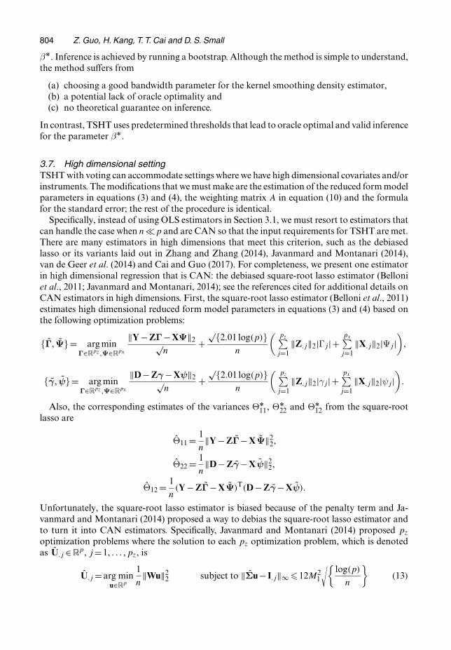
Specifically, instead of using OLS estimators in Section 3.1, we must resort to estimators thatcan handle the case when np and are CAN so that the input requirements for TSHT are met.There are many estimators in high dimensions that meet this criterion, such as the debiasedlasso or its variants laid out in Zhang and Zhang (2014), Javanmard and Montanari (2014),van de Geer et al. (2014) and Cai and Guo (2017). For completeness, we present one estimatorin high dimensional regression that is CAN: the debiased square-root lasso estimator (Belloniet al., 2011; Javanmard and Montanari, 2014); see the references cited for additional details onCAN estimators in high dimensions. First, the square-root lasso estimator (Belloni et al., 2011)estimates high dimensional reduced form model parameters in equations (3) and (4) based onthe following optimization problems:

{Γ, Ψ}= arg minΓ∈Rpz ,Ψ∈Rpx

‖Y −ZΓ−XΨ‖2√n

+√{2:01 log.p/}

n

(pz∑

j=1‖Z:j‖2|Γj|+

px∑j=1

‖X:j‖2|Ψj|)

,

{γ, ψ}= arg minΓ∈Rpz ,Ψ∈Rpx

‖D−Zγ−Xψ‖2√n

+√{2:01 log.p/}

n

(pz∑

j=1‖Z:j‖2|γj|+

px∑j=1

‖X:j‖2|ψj|)

:

Also, the corresponding estimates of the variances ΘÅ11, ΘÅ

22 and ΘÅ12 from the square-root

lasso are

Θ11 = 1n‖Y −ZΓ−XΨ‖2

2,

Θ22 = 1n‖D−Zγ−Xψ‖2

2,

Θ12 = 1n

.Y −ZΓ−XΨ/T.D−Zγ−Xψ/:

Unfortunately, the square-root lasso estimator is biased because of the penalty term and Ja-vanmard and Montanari (2014) proposed a way to debias the square-root lasso estimator andto turn it into CAN estimators. Specifically, Javanmard and Montanari (2014) proposed pz

optimization problems where the solution to each pz optimization problem, which is denotedas U:j ∈Rp, j =1, : : : , pz, is

U:j =arg minu∈Rp

1n‖Wu‖2

2 subject to ‖Σu − I:j‖∞ �12M21

√{log.p/

n

}.13/


with Σ= .1=n/WTW. Here, I:j denotes the jth column of the identity matrix I and M1 denotesthe largest eigenvalue of ΣÅ. Let U denote the matrix concatenation of the pz solutions to theoptimization problem. Then, the debiased estimates of Γ and γ, which are denoted as Γ and γ,are

Γ= Γ+ 1n

UWT.Y −ZΓ−XΨ/,

γ= γ+ 1n

UWT.D−Zγ−Xψ/:

.14/

We now have obtained all the ingredients for TSHT in the high dimensional setting:

(a) the CAN estimators ofΓÅ andγÅ, Γ and γ respectively, based on the debiased square-rootlasso;

(b) consistent estimators of the error variances ΘÅ11, ΘÅ

22 and ΘÅ12, Θ11, Θ22 and Θ12 respecti-

vely, from the square-root lasso;(c) an estimate of the precision matrix of W, U from the debiasing procedure.

Running TSHT with these inputs will estimate the set of valid instruments V in high dimensionalsettings.

For point estimation of βÅ in high dimensions, we simply replace A in equation (10) with theidentity matrix

β= γTV ΓVγT

V γV: .15/

The variance estimate of the estimator in equation (15) uses a high dimensional estimate of theprecision matrix in equation (11), i.e.

var=γT

V .U·,V /T

.WTW=n/U:,V γV

.γTV γV /2

.Θ11 + β2Θ22 −2β Θ12/: .16/

Given the point estimate and the variance, the confidence interval for βÅ follows the usual form

.β− z1−α=2√

.var=n/, β+ z1−α=2√

.var=n//: .17/

4. Theoretical results

In this section, we state the asymptotic properties of TSHT with voting. In Section 4.1, weconsider the low dimensional setting where px and pz are fixed. In Section 4.2, we consider thegeneral case when px and/or pz are allowed to grow and exceed sample size n.

4.1. Invalid instrumental variables in low dimensional settingFirst, we prove that the estimated set V is an asymptotically consistent estimator of the true setVÅ in the low dimensional setting where px and pz are fixed.

Lemma 1. Under the plurality rule assumption, limn→∞ P.V =VÅ/=1.

Lemma 1 confirms our intuition in Section 3.4 that the voting process correctly generates theset of instruments that are relevant and valid. In fact, a useful feature of our method is that itprovably and correctly selects the IVs that satisfy assumptions 1–3, which is something that is


not possible with prior methods that target only βÅ, e.g. the median method. Next, theorem 2states that the confidence interval that was outlined in Section 3.5 has the desired coverage andoptimal length in the low dimensional settings with fixed px and pz.

Theorem 2. Suppose that the plurality rule assumption holds. Then, as n→∞, we have

√n.βL −βÅ/

d→N

{0,

σ2

γÅTVÅ .ΣÅ

VÅVÅ −ΣÅVÅ.VÅ/CΣÅ−1

.VÅ/C.VÅ/CΣÅ.VÅ/CVÅ/γÅ

VÅ

}: .18/

Consequently, the confidence interval that is given in equation (12) has asymptotic coverageprobability 1−α, i.e.

P{βÅ ∈ .βL − z1−α=2

√.varL=n/, βL + z1−α=2

√.varL=n//

}→1−α: .19/

We note that the proposed estimator βL has the same asymptotic variance as the oracle TSLSestimator with prior knowledge of VÅ, which is efficient under the homoscedastic varianceassumption; see theorem 5.2 in Wooldridge (2010) for details. Consequently, our confidenceinterval in equation (12) asymptotically performs like the oracle TSLS confidence interval andis of optimal length. But, unlike TSLS, we achieve this oracle performance without prior knowl-edge of VÅ. We remind readers that the previous estimators that were proposed by Bowden et al.(2015, 2016), Burgess et al. (2016) and Kang et al. (2016a) do not achieve oracle performanceand TSLS-like efficiency whereas the estimator that was proposed by Windmeijer et al. (2016)does achieve this, but only when the 50% rule condition holds.

4.2. Invalid instrumental variables in high dimensional settingWe now consider the asymptotic properties of TSHT with voting under the general case whenpz and/or px are allowed to grow, potentially exceeding sample size n. As noted in Section3.2, to be in alignment with the traditional high dimensional literature where pz and/or px arealways larger than n and growing faster than n, we simplify TSHT by replacing the thresholdsin equations (5) and (7) from log.max{pz, n}/ to log.pz/.

We first introduce the regularity assumptions that are used in high dimensional statistics(Bickel et al., 2009; Buhlmann and van de Geer, 2011; Cai and Guo, 2017).

Assumption 4 (coherence). The matrix ΣÅ satisfies 1=M1 �λmin.ΣÅ/ �λmax.ΣÅ/ � M1 forsome constant M1 �1 and has bounded sub-Gaussian norm.

Assumption 5 (normality). The error terms in equations (3) and (4) follow a bivariate normaldistribution.

Assumption 6 (global IV strength). The IVs are globally strong with√{.γÅ

VÅ/TΣVÅ,VÅγÅVÅ}�

sz1 log.p/=√

n, where VÅ is the set of valid IVs defined in definition 3.

Assumption 4 makes sure that the spectrum of the design matrix W is well behaved as p→∞.Assumption 5 is made out of simplicity, similarly to the normal error assumption that is made inthe work on inference in the weak IV literature (e.g. section 2 of Moreira (2003) and section 2.2.1of Andrews et al. (2007)) and in high dimensional linear models (e.g. theorem 2.5 in Javanmardand Montanari (2014) and theorem 2.1 in van de Geer et al. (2014)). Finally, assumption 6bounds the global strength of the instruments, measured by the weighted l2-norm of γÅ

VÅ , awayfrom zero. Assumption 6 is commonly assumed in the traditional IV literature under the guiseof a concentration parameter, which is a measure of instrument strength and is the weightedl2-norm of γÅ

VÅ (Stock et al., 2002; Wooldridge, 2010), and in the high dimensional IV literature


Belloni et al. (2012) and Chernozhukov et al. (2015). Sections B and C in the on-line supplemen-tary materials provide additional discussions and show that, if the IVs are valid, then regularityassumptions 4–6 are sufficient to construct valid confidence intervals in high dimensions.

When IVs are invalid, we need to make two additional assumptions that are not part of thehigh dimensional statistics or IVs literature and may be of theoretical interest in future work.

Assumption 7 (individual IV strength). For IVs in SÅ, δmin =minj∈SÅ |γÅj |�√{log.pz/=n}.

Assumption 8 (separated levels of violation). For the pair j, k ∈SÅ with πÅj =γÅ

j �=πÅk =γÅ

k ,∣∣∣∣πÅj

γÅj

− πÅk

γÅk

∣∣∣∣� 12.1+maxj∈SÅ |ΓÅj =γÅ

j |/δmin

√{M1 log.pz/

λmin.ΘÅ/n

}: .20/

Assumption 8 bounds individual IV strength away from zero so that all IVs in selected Sare strong. Without this condition, an individually weak IV with small γj may be included inthe first thresholding step and subsequently cause trouble to the second thresholding step inequation (7) that uses γj in the denominator to construct a candidate estimate of πÅ and PÅ. Inthe literature, assumption 8 is similar to the ‘beta-min’-assumption in high dimensional linearregression without IVs, with the exception that this condition is not imposed on our inferentialquantity of interest, βÅ. Also, assumption 8 is different from assumption 6 in that assumption 6requires only the global IV strength to be bounded away from zero. Next, assumption 9 requiresthat the difference between different levels of ratios πÅ

j =γÅj is sufficiently large. Without this

assumption, it would be difficult to distinguish subsets of instruments with different πÅj =γÅ

j -values from the data and to identify the set of valid IVs based on the plurality rule. For example,consider instruments k and j with πÅ

k =γÅk �=πÅ

j =γÅj . If equation (20) is satisfied, then k �∈ P [j]

with high probability because πÅk =γÅ

k and πÅj =γÅ

j are far apart from each other. In contrast, ifequation (20) does not hold, then P [j]

might contain instrument k by chance because πÅk =γÅ

k

and πÅj =γÅ

j are close to each other.Lemma 2 shows that, with assumptions 4–6 and 8 and 9 and the plurality rule condition,

TSHT with voting produces a consistent estimator of the set of valid instruments in the highdimensional setting.

Lemma 2. Suppose that s√

sz1log.p/=√

n → 0 and assumptions 4–6, and 8 and 9 and theplurality rule condition are satisfied. With probability larger than 1−c{p−c +exp .−cn/} forsome c> 0, V =VÅ.

Next, the following theorem shows that β is a consistent and asymptotic normal estimator ofβÅ.

Theorem 3. Under the same assumption as lemma 2, we have

√n.β−βÅ/=T β

Å +ΔβÅ.21/

where T βÅ |W ∼ N.0, var/ and var = σ2γT

VÅ.U·,VÅ/TWTWU:,VÅγVÅ=n.γTVÅγVÅ/2. As

s√

sz1log.p/=√

n → 0, ΔβÅ=√

var→p 0 and the confidence interval that is given in equation(17) has asymptotic coverage probability of 1−α, i.e.

P{βÅ ∈ .β− z1−α=2√

.var=n/, β+ z1−α=2√

.var=n//}→1−α: .22/


5. Simulation

5.1. Set-up: low dimensional settingIn addition to the theoretical analysis of our method in Section 4, we also conduct a simulationstudy to investigate the numerical performance of our method. The design of the simulationstudy follows closely that of Windmeijer et al. (2016) where we use models (2) and (3) in Section2.1. Specifically,

(a) there are pz =7 or pz =10 instruments,(b) there are no covariates,(c) the instruments are generated from a multivariate normal distribution with mean 0 and

identity covariance,(d) the treatment effect is fixed to be βÅ =1 and(e) the errors have variance 1 and covariance 0:25.

Similarly to Windmeijer et al. (2016), we vary

(a) the sample size n,(b) the strength of the IV by manipulating γÅ = .1, : : : , 1/Cγ with different values of Cγ and(c) the degree of violations of assumptions 2 and 3 by manipulating πÅ.

With respect to the last variation, if pz = 7, we set πÅ = .1, 1, 0:5, 0:5, 0, 0, 0/Cπ where Cπ is aconstant that we vary to change the magnitude ofπÅ. If pz =10, we setπÅ = .1, 1, 1, 0, : : : , 0/Cπ.The first setting mimics the case where the 50% rule condition holds, similarly to Windmeijeret al. (2016), whereas the second setting mimics the case where the 50% rule fails but the pluralityrule condition holds.

Under this data-generating mechanism, we compare our procedure TSHT with voting with

(a) the naive TSLS that assumes that all the instruments satisfy assumptions 1–3,(b) the oracle TSLS that knows, a priori, which instruments satisfy assumptions 1–3,(c) the method of Windmeijer et al. (2016) that uses the adaptive lasso tuned via cross-

validation and the initial median estimator and(d) the unweighted median estimator of Bowden et al. (2016) and Burgess et al. (2016) with

bootstrapped confidence intervals by using the R package MendelianRandomization(Yavorska and Burgess, 2017) under default settings.

For (a), we implement TSLS so that it mimics most practitioners’ use of TSLS by simplyassuming that all the instruments Z are valid. For (b), we have the oracle TSLS where an oracleprovides us with the true set of valid IVs, which will not occur in practice. Because TSLS is notrobust against weak instruments, we purposely set our Cγ to correspond to strong IV regimes.Finally, for (c) and (d), see Section 3.6 for discussions of the methods. Our simulations arerepeated 500 times and we measure the median absolute error, the empirical coverage proportionand the average length of the confidence interval computed across simulations.

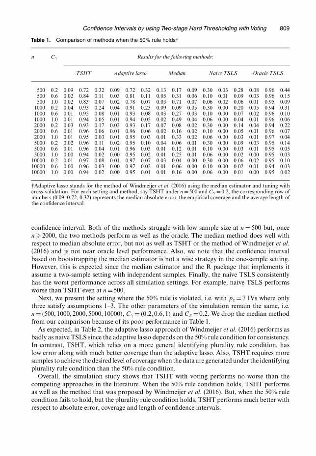
5.2. Low dimensional settingWe first present the setting where the 50% rule holds. Specifically, following Windmeijer et al.(2016), Table 1 shows the cases where we have 10 IVs with sz2 = 3, n = .500, 1000, 2000, 5000,10000/, Cγ = .0:2, 0:6, 1/ and Cπ = 0:2. For reference, with n = 500, 2000, 5000 and Cγ = 0:2,the expected concentration parameter is 7nC2

γ , or, for each n, 140, 560 and 1400 respectively.Because the 50% rule condition holds, TSHT, the method of Windmeijer et al. (2016) and themedian method should do well. Indeed, between TSHT and the method of Windmeijer et al.(2016), there is little difference in terms of median absolute error, coverage and length of the


Table 1. Comparison of methods when the 50% rule holds†

n Cγ Results for the following methods:

TSHT Adaptive lasso Median Naive TSLS Oracle TSLS

500 0.2 0.09 0.72 0.32 0.09 0.72 0.32 0.13 0.17 0.09 0.30 0.03 0.28 0.08 0.96 0.44500 0.6 0.02 0.84 0.11 0.03 0.81 0.11 0.05 0.31 0.06 0.10 0.01 0.09 0.03 0.96 0.15500 1.0 0.02 0.83 0.07 0.02 0.78 0.07 0.03 0.71 0.07 0.06 0.02 0.06 0.01 0.95 0.09

1000 0.2 0.04 0.93 0.24 0.04 0.91 0.23 0.09 0.09 0.05 0.30 0.00 0.20 0.05 0.94 0.311000 0.6 0.01 0.95 0.08 0.01 0.93 0.08 0.03 0.27 0.03 0.10 0.00 0.07 0.02 0.96 0.101000 1.0 0.01 0.94 0.05 0.01 0.94 0.05 0.02 0.49 0.04 0.06 0.00 0.04 0.01 0.96 0.062000 0.2 0.03 0.93 0.17 0.03 0.93 0.17 0.07 0.08 0.02 0.30 0.00 0.14 0.04 0.94 0.222000 0.6 0.01 0.96 0.06 0.01 0.96 0.06 0.02 0.16 0.02 0.10 0.00 0.05 0.01 0.96 0.072000 1.0 0.01 0.95 0.03 0.01 0.95 0.03 0.01 0.33 0.02 0.06 0.00 0.03 0.01 0.97 0.045000 0.2 0.02 0.96 0.11 0.02 0.95 0.10 0.04 0.06 0.01 0.30 0.00 0.09 0.03 0.95 0.145000 0.6 0.01 0.96 0.04 0.01 0.96 0.03 0.01 0.12 0.01 0.10 0.00 0.03 0.01 0.95 0.055000 1.0 0.00 0.94 0.02 0.00 0.95 0.02 0.01 0.25 0.01 0.06 0.00 0.02 0.00 0.95 0.03

10000 0.2 0.01 0.97 0.08 0.01 0.97 0.07 0.03 0.04 0.00 0.30 0.00 0.06 0.02 0.95 0.1010000 0.6 0.00 0.96 0.03 0.00 0.97 0.02 0.01 0.06 0.00 0.10 0.00 0.02 0.01 0.94 0.0310000 1.0 0.00 0.94 0.02 0.00 0.95 0.01 0.01 0.16 0.00 0.06 0.00 0.01 0.00 0.95 0.02

†Adaptive lasso stands for the method of Windmeijer et al. (2016) using the median estimator and tuning withcross-validation. For each setting and method, say TSHT under n=500 and Cγ =0:2, the corresponding row ofnumbers (0.09, 0.72, 0.32) represents the median absolute error, the empirical coverage and the average length ofthe confidence interval.

confidence interval. Both of the methods struggle with low sample size at n = 500 but, oncen � 2000, the two methods perform as well as the oracle. The median method does well withrespect to median absolute error, but not as well as TSHT or the method of Windmeijer et al.(2016) and is not near oracle level performance. Also, we note that the confidence intervalbased on bootstrapping the median estimator is not a wise strategy in the one-sample setting.However, this is expected since the median estimator and the R package that implements itassume a two-sample setting with independent samples. Finally, the naive TSLS consistentlyhas the worst performance across all simulation settings. For example, naive TSLS performsworse than TSHT even at n=500.

Next, we present the setting where the 50% rule is violated, i.e. with pz = 7 IVs where onlythree satisfy assumptions 1–3. The other parameters of the simulation remain the same, i.e.n= .500, 1000, 2000, 5000, 10000/, Cγ = .0:2, 0:6, 1/ and Cπ =0:2. We drop the median methodfrom our comparison because of its poor performance in Table 1.

As expected, in Table 2, the adaptive lasso approach of Windmeijer et al. (2016) performs asbadly as naive TSLS since the adaptive lasso depends on the 50% rule condition for consistency.In contrast, TSHT, which relies on a more general identifying plurality rule condition, haslow error along with much better coverage than the adaptive lasso. Also, TSHT requires moresamples to achieve the desired level of coverage when the data are generated under the identifyingplurality rule condition than the 50% rule condition.

Overall, the simulation study shows that TSHT with voting performs no worse than thecompeting approaches in the literature. When the 50% rule condition holds, TSHT performsas well as the method that was proposed by Windmeijer et al. (2016). But, when the 50% rulecondition fails to hold, but the plurality rule condition holds, TSHT performs much better withrespect to absolute error, coverage and length of confidence intervals.


Table 2. Comparison of methods when the 50% rule is violated but the plurality rule holds†

n Cγ Results for the following methods:

TSHT Adaptive lasso Naive TSLS Oracle TSLS

500 0.2 0.37 0.17 0.38 0.35 0.18 0.39 0.41 0.00 0.33 0.09 0.97 0.51500 0.6 0.11 0.24 0.13 0.13 0.17 0.13 0.14 0.00 0.11 0.03 0.93 0.17500 1.0 0.07 0.21 0.08 0.08 0.18 0.08 0.09 0.00 0.07 0.02 0.94 0.10

1000 0.2 0.37 0.17 0.36 0.37 0.10 0.33 0.42 0.00 0.24 0.07 0.96 0.361000 0.6 0.09 0.32 0.13 0.12 0.12 0.11 0.14 0.00 0.08 0.02 0.96 0.121000 1.0 0.06 0.24 0.07 0.07 0.11 0.07 0.09 0.00 0.05 0.01 0.93 0.072000 0.2 0.19 0.45 0.32 0.44 0.01 0.27 0.42 0.00 0.17 0.05 0.95 0.252000 0.6 0.04 0.62 0.10 0.15 0.02 0.09 0.14 0.00 0.06 0.01 0.94 0.082000 1.0 0.03 0.55 0.06 0.09 0.02 0.05 0.09 0.00 0.03 0.01 0.94 0.055000 0.2 0.04 0.90 0.19 0.49 0.00 0.19 0.42 0.00 0.11 0.03 0.95 0.165000 0.6 0.01 0.91 0.06 0.17 0.00 0.06 0.14 0.00 0.03 0.01 0.94 0.055000 1.0 0.01 0.91 0.04 0.10 0.00 0.04 0.09 0.00 0.02 0.01 0.94 0.03

10000 0.2 0.02 0.92 0.13 0.50 0.00 0.14 0.43 0.00 0.07 0.02 0.96 0.1110000 0.6 0.01 0.92 0.04 0.17 0.00 0.04 0.14 0.00 0.02 0.01 0.95 0.0410000 1.0 0.00 0.94 0.03 0.10 0.00 0.03 0.09 0.00 0.01 0.00 0.94 0.02

†Adaptive lasso stands for the method of Windmeijer et al. (2016) using the median estimator and tuning withcross-validation. For each setting and method, say TSHT under n=500 and Cγ =0:2, the corresponding row ofnumbers (0.37, 0.17, 0.38) represents the median absolute error, the empirical coverage and the average length ofthe confidence interval.

5.3. High dimensional settingIn this section, we present simulations in high dimensions. We use the same data-generatingmodels as before, except that we have pz =100 instruments with the first sz1 =7 being relevantand the first sz2 =5 being valid. We also have px =150 covariates with sx2 = sx1 =10. We refer tothis case as the high dimensional instruments and covariates setting. We also consider pz =9 andpx =150, which we refer to as the low dimensional instruments and high dimensional covariatessetting. The only difference between these two settings is the dimension of IVs. However, froma theoretical standpoint, both settings are considered high dimensional.

Both the instruments and the covariates Wi: are generated from a multivariate normal withmean 0 and covariance ΣÅ

ij =0:5|i−j| for 1� i, j �px +pz. The other parameters for the modelsare βÅ =1, φÅ = .0:6, 0:7, 0:8, : : : , 1:5, 0, 0, : : : , 0/∈R150, ψÅ = .1:1, 1:2, 1:3, : : : , 2:0, 0, 0, : : : , 0/∈R150, var.εi1/=var.εi2/=1:5 and cov.εi1, εi2/=0:75. We vary

(a) the sample size n,(b) the strength of IV via γÅ and(c) the degree of violations of assumptions 2 and 3 via πÅ.

For the sample size, we let n= .200, 300, 1000, 2500/. For the IV strength, we set γÅ =Cγ.1, 1, 1,1, 1, 1, 1, 0, 0, : : : , 0/ with Cγ=0:5. For violations of assumptions 2 and 3, we setπÅ = .0, 0, 0, 0, 0,1, 1, 0, 0, : : : , 0/Cπ where Cπ is a constant that we vary to change the magnitude of πÅ.

We compare TSHT with the oracle TSLS method where the oracle uses only the relevant andvalid instruments, i.e. knows the seven relevant instruments, of which the first five are valid.We do not include the naive TSLS method because it is not feasible in high dimensions. Wealso do not include other methods because they were not designed with high dimensionality inmind. The high dimensional instruments and covariate setting is presented in Table 3 whereasthe low dimensional instruments and high dimensional covariates setting is presented in Table 4.


Table 3. Performance of TSHT in high dimensional instruments andcovariates with px D150 and pz D100†

n Cπ Results for TSHT Results for oracle

200 0.25 0.162 0.162 0.202 0.038 0.956 0.219200 0.50 0.129 0.448 0.232 0.036 0.962 0.218200 1.00 0.056 0.876 0.259 0.036 0.956 0.221300 0.25 0.155 0.080 0.164 0.033 0.952 0.179300 0.50 0.093 0.516 0.197 0.029 0.952 0.177300 1.00 0.041 0.906 0.209 0.029 0.946 0.176

1000 0.25 0.136 0.062 0.094 0.016 0.936 0.0961000 0.50 0.020 0.942 0.119 0.016 0.936 0.0951000 1.00 0.020 0.958 0.120 0.016 0.964 0.0962500 0.25 0.015 0.802 0.068 0.011 0.946 0.0602500 0.50 0.012 0.956 0.069 0.011 0.948 0.0602500 1.00 0.011 0.954 0.069 0.010 0.942 0.060

†For each setting and method, say TSHT under n=200 and Cπ =0.25,the row of numbers (0.162, 0.162, 0.202) represents the median abso-lute error, the empirical coverage and average length of the confidenceinterval.

To mimic the low dimensional results, Table 3 presents the result for Cπ = .0:25, 0:5, 1/. In bothsettings, for n=200, our TSHT method does not achieve the desired level of coverage, althoughcoverage improves dramatically once the violation of assumptions 2 and 3 becomes bigger, i.e.when Cπ =1. When n�300 and if the violations of assumptions 2 and 3 are substantial, TSHTachieves the desired level of coverage with absolute error and length of the confidence intervalthat are comparable with those of the oracle.

6. Application: causal effect of years of education on annual earnings

To demonstrate our method in a real setting, we analyse the causal effect of years of education onyearly earnings, which has been studied extensively in economics by using IV methods (Angristand Krueger, 1991; Card, 1993, 1999). The data come from the WLS, which is a longitudinalstudy that has kept track of American high school graduates from Wisconsin since 1957, andwe examine the relationship between graduates’ earnings and education from the 1974 survey(Hauser, 2005), roughly 20 years after they graduated from high school. Our analysis includesN =3772 individuals, 1784 males and 1988 females. For our outcome, we use imputed log(totalyearly earnings) prepared by the WLS (see WLS documentation and Hauser (2005) for details)and, for the treatment, we use the total years of education, all from the 1974 survey. The mediantotal earnings is $9200 with a 25% quartile of $1000 and a 75% quartile of $15320 in 1974dollars. The mean time of total education is 13.7 years with a standard deviation of 2.3 years.

We incorporate many covariates, including sex, graduate’s home town population, educationalattainment of the graduates’ parents, graduates’ family income, relative income in graduates’home town, graduates’ high school denomination and high school class size, all measured in1957 when the participants were high school seniors. We also include 81 genetic covariates,specifically single-nucleotide polymorphisms, that were part of the WLS to control further forpotential variations between graduates; see section D in the on-line supplementary materials fordetails on the non-genetic and genetic covariates. In summary, our data analysis includes sevennon-genetic covariates and 81 genetic covariates. We used five instruments in our analysis, all


Table 4. Performance ofTSHT in low dimension instruments (pz D9)and high dimension covariates (px D150)†

n Cπ Results for TSHT Results for oracle

200 0.25 0.169 0.196 0.214 0.037 0.928 0.221200 0.50 0.167 0.362 0.240 0.039 0.926 0.221200 1.00 0.057 0.852 0.276 0.041 0.942 0.222300 0.25 0.155 0.094 0.170 0.031 0.938 0.178300 0.50 0.123 0.426 0.198 0.031 0.956 0.177300 1.00 0.043 0.916 0.222 0.030 0.960 0.177

1000 0.25 0.133 0.076 0.090 0.015 0.944 0.0951000 0.50 0.019 0.962 0.113 0.016 0.954 0.0961000 1.00 0.020 0.958 0.113 0.016 0.950 0.0952500 0.25 0.012 0.860 0.067 0.009 0.948 0.0602500 0.50 0.012 0.952 0.068 0.010 0.950 0.0602500 1.00 0.012 0.958 0.068 0.011 0.944 0.060

†For each setting and method, say TSHT under n=200 and Cπ =0:25,the row of numbers (0.169, 0.196, 0.214) represents the median absoluteerror, the empirical coverage and the average length of the confidenceinterval.

derived from past studies of education on earnings (Card, 1993; Blundell et al., 2005; Gary-Boboet al., 2006). They are

(a) total number of sisters,(b) total number of brothers,(c) individuals, birth order in the family, all from Gary-Bobo et al. (2006),(d) proximity to college from Card (1993) and(e) teachers’ interest in individual’s college education from Blundell et al. (2005),

all measured in 1957. Although all these IVs have been suggested to be valid with varyingexplanations why they satisfy assumptions 2 and 3 after controlling for the aforementionedcovariates, in practice, we are always uncertain because of the lack of complete socio-economicknowledge about the effect of these IVs. Our method should provide some protection againstthis uncertainty compared with traditional methods where they simply assume that all five IVsare valid. Also, the first-stage F -test produces an F -statistic of 90.3 with a p-value less than10−16, which indicates a very strong set of instruments. For more details on the instruments, seesection D of the on-line supplementary materials.

When we use OLS where we run a regression of the treatment and the covariates on the out-come and looking at the slope coefficient of the treatment variable, we find the effect estimate tobe 0.097 (95% confidence interval 0.051, 0.143). This agrees with previous literature which sug-gests a statistically significant positive association between years of education and log-earnings(Card, 1999). However, OLS does not completely control for confounding even after controllingfor covariates. TSLS provides an alternative method of controlling for confounding by using in-struments so long as all the five instruments satisfy the three core assumptions and the inclusionof covariates helps to make these assumptions more plausible. The TSLS estimate is 0.169 (95%confidence interval 0.029, 0.301), which is inconsistent with previous studies’ estimates amongindividuals from the USA between the 1950s and the 1970s, which range from 0.06 to 0.13 (seeTable 4 in Card (1999)). Our method, which addresses the concern for invalid instruments withTSLS, provides an estimate of 0.062 (95% confidence interval 0.046, 0.077), which is more con-sistent with previous studies’ estimates of the effect of years of education on earnings. The data


analysis suggests that our method can be a useful tool in IV analysis when there is concern forinvalid instruments, even after attempting to mitigate this problem via covariates. Our methodprovides more accurate estimates of the returns on education than does TSLS, which naivelyassumes that all the instruments are valid.

7. Conclusion and discussion

We present a method to estimate the effect of the treatment on the outcome by using IVs wherewe do not make the assumption that all the instruments are valid. Our approach is based onthe novel TSHT procedure with majority and plurality voting. We theoretically show that ourapproach succeeds in selecting valid IVs in the presence of possibly invalid IVs even when the50% rule is violated and produces robust confidence intervals. In simulation and in real datasettings, our approach provides a more robust analysis than the traditional IV approaches orrecent methods in the invalid IV literature by providing some protection against possibly invalidinstruments and reaches oracle performance around n � 2000. Overall, we believe that ourmethod can be a valuable tool for researchers in Mendelian randomization and IVs wheneverthere are concerns for invalid IVs, which is often the case in practice.

Finally, our theoretical analysis for the case of invalid IVs in high dimensions require assump-tions 8 and 9. We believe that assumption 9 is probably necessary for the invalid IV problemin high dimensions because of the model selection literature by Leeb and Potscher (2005) whopointed out that ‘in general no model selector can be uniformly consistent for the most parsimo-nious true model’ and hence that the post-model-selection inference is generally non-uniform.Consequently, the set of competing models must be ‘well separated’ such that we can consistentlyselect a correct model. Assumption 9 serves as this ‘well-separated’ condition in our invalid IVproblem. Although some recent work in high dimensional inference (Zhang and Zhang, 2014;Javanmard and Montanari, 2014; van de Geer et al., 2014; Chernozhukov et al., 2015; Cai andGuo, 2017) does not make this well-separated assumption, our invalid IV problem is differentfrom the prior work because a single invalid IV declared as valid can ruin inference whereas thesaid prior works assume that the moment conditions are known perfectly. Advanced methodsmay weaken assumption 9 and we leave this as a direction for further research.

Acknowledgements

The research of Hyunseung Kang was supported in part by National Science Foundation grantDMS-1502437. The research of T. Tony Cai was supported in part by National Science Foun-dation grants DMS-1208982 and DMS-1403708, and National Institutes of Health grant R01CA127334. The research of Dylan S. Small was supported in part by National Science Foun-dation grant SES-1260782.

References

Andrews, D. W. K., Moreira, M. J. and Stock, J. H. (2007) Performance of conditional Wald tests in IV regressionwith weak instruments. J. Econmetr., 139, 116–132.

Angrist, J. D., Imbens, G. W. and Rubin, D. B. (1996) Identification of causal effects using instrumental variables.J. Am. Statist. Ass., 91, 444–455.

Angrist, J. D. and Krueger, A. B. (1991) Does compulsory school attendance affect schooling and earnings? Q. J.Econ., 106, 979–1014.

Baiocchi, M., Cheng, J. and Small, D. S. (2014) Instrumental variable methods for causal inference. Statist. Med.,33, 2297–2340.

Belloni, A., Chen, D., Chernozhukov, V. and Hansen, C. (2012) Sparse models and methods for optimal instru-ments with an application to eminent domain. Econometrica, 80, 2369–2429.


Belloni, A., Chernozhukov, V. and Hansen, C. (2014) Inference on treatment effects after selection among high-dimensional controls. Rev. Econ. Stud., 81, 608–650.

Belloni, A., Chernozhukov, V. and Wang, L. (2011) Square-root lasso: pivotal recovery of sparse signals via conicprogramming. Biometrika, 98, 791–806.

Bickel, P. J., Ritov, Y. and Tsybakov, A. B. (2009) Simultaneous analysis of lasso and Dantzig selector. Ann.Statist., 37, 1705–1732.

Blundell, R., Dearden, L. and Sianesi, B. (2005) Evaluating the effect of education on earnings: models, methodsand results from the National Child Development Survey. J. R. Statist. Soc. A, 168, 473–512.

Bowden, J., Davey Smith, G. and Burgess, S. (2015) Mendelian randomization with invalid instruments: effectestimation and bias detection through egger regression. Int. J. Epidem., 44, 512–525.

Bowden, J., Davey Smith, G., Haycock, P. C. and Burgess, S. (2016) Consistent estimation in Mendelian random-ization with some invalid instruments using a weighted median estimator. Genet. Epidem., 40, 304–314.

Buhlmann, P. and van de Geer, S. (2011) Statistics for High-dimensional Data: Methods, Theory and Applications.Berlin: Springer.

Burgess, S., Bowden, J., Dudbridge, F. and Thompson, S. G. (2016) Robust instrumental variable methods usingmultiple candidate instruments with application to Mendelian randomization. arXiv Preprint. University ofCambridge, Cambridge.

Burgess, S., Timpson, N. J., Ebrahim, S. and Davey Smith, G. (2015) Mendelian randomization: where are wenow and where are we going? Int. J. Epidem., 44, 379–388.

Cai, T. T. and Guo, Z. (2017) Confidence intervals for high-dimensional linear regression: minimax rates andadaptivity. Ann. Statist., 45, 615–646.

Card, D. (1993) Using geographic variation in college proximity to estimate the return to schooling. WorkingPaper 4483. National Bureau of Economic Research, Cambridge.

Card, D. (1999) The causal effect of education on earnings. In Handbook of Labor Economics (eds O. C. Ashenfelterand D. Card), vol. 3, part A, ch. 30, pp. 1801–1863. New York: Elsevier.

Cheng, X. and Liao, Z. (2015) Select the valid and relevant moments: an information-based lasso for GMM withmany moments. J. Econmetr., 186, 443–464.

Chernozhukov, V., Hansen, C. and Spindler, M. (2015) Post-selection and post-regularization inference in linearmodels with many controls and instruments. Am. Econ. Rev., 105, 486–490.

Davey Smith, G. and Ebrahim, S. (2003) Mendelian randomization: can genetic epidemiology contribute tounderstanding environmental determinants of disease? Int. J. Epidem., 32, 1–22.

Davey Smith, G. and Ebrahim, S. (2004) Mendelian randomization: prospects, potentials, and limitations. Int. J.Epidem., 33, 30–42.

Donoho, D. L. (1995) De-noising by soft-thresholding. IEEE Trans. Inform. Theory, 41, 613–627.Donoho, D. L. and Johnstone, J. M. (1994) Ideal spatial adaptation by wavelet shrinkage. Biometrika, 81, 425–455.Fan, J. and Liao, Y. (2014) Endogeneity in high dimensions. Ann. Statist., 42, 872–917.Gary-Bobo, R., Picard, N. and Prieto, A. (2006) Birth order and sibship sex composition as instruments in the

study of education and earnings. Discussion Paper 5514. Centre for Economic and Policy Research, London.Gautier, E. and Tsybakov, A. B. (2011) High-dimensional instrumental variables regression and confidence sets.

Preprint arXiv:1105.2454. Center for Research in Economics and Statistics, Malakoff.van de Geer, S., Buhlmann, P., Ritov, Y. and Dezeure, R. (2014) On asymptotically optimal confidence regions

and tests for high-dimensional models. Ann. Statist., 42, 1166–1202.Han, C. (2008) Detecting invalid instruments using l 1-gmm. Econ. Lett., 101, 285–287.Hartwig, F. P., Davey Smith, G. and Bowden, J. (2017) Robust inference in summary data Mendelian randomiza-

tion via the zero modal pleiotropy assumption. Int. J. Epidem., 46, 1985–1998.Hastie, T., Tibshirani, R. and Friedman, J. (2016) The Elements of Statistical Learning: Data Mining, Inference,

and Prediction, 3rd edn. New York: Springer.Hauser, R. M. (2005) Survey response in the long run: the Wisconsin longitudinal study. Fld Meth., 17, 3–29.Hernan, M. A. and Robins, J. M. (2006) Instruments for causal inference: an epidemiologist’s dream? Epidemiol-

ogy, 17, 360–372.Holland, P. W. (1988) Causal inference, path analysis, and recursive structural equations models. Sociol. Methodol.,

18, 449–484.Imbens, G. W. (2014) Instrumental variables: an econometrician’s perspective. Statist. Sci., 29, 323–358.Imbens, G. W. and Angrist, J. D. (1994) Identification and estimation of local average treatment effects. Econo-

metrica, 62, 467–475.Javanmard, A. and Montanari, A. (2014) Confidence intervals and hypothesis testing for high-dimensional re-

gression. J. Mach. Learn. Res., 15, 2869–2909.Kang, H., Cai, T. T. and Small, D. S. (2016a) A simple and robust confidence interval for causal effects with possibly

invalid instruments. Preprint arXiv:1504.03718. Department of Statistics, University of Wisconsin—Madison,Madison.

Kang, H., Zhang, A., Cai, T. T. and Small, D. S. (2016b) Instrumental variables estimation with some invalidinstruments and its application to Mendelian randomization. J. Am. Statist. Ass., 111, 132–144.

Kolesar, M., Chetty, R., Friedman, J. N., Glaeser, E. L. and Imbens, G. W. (2015) Identification and inferencewith many invalid instruments. J. Bus. Econ. Statist., 33, 474–484.


Lawlor, D. A., Harbord, R. M., Sterne, J. A. C., Timpson, N. and Davey Smith, G. (2008) Mendelian random-ization: using genes as instruments for making causal inferences in epidemiology. Statist. Med., 27, 1133–1163.

Leeb, H. and Potscher, B. M. (2005) Model selection and inference: facts and fiction. Econmetr. Theory, 21, 21–59.Moreira, M. J. (2003) A conditional likelihood ratio test for structural models. Econometrica, 71, 1027–1048.Murray, M. P. (2006) Avoiding invalid instruments and coping with weak instruments. J. Econ. Perspect., 20,

111–132.Neyman, J. (1923) On the application of probability theory to agricultural experiments: Essay on principles,

section 9. Statist. Sci., 5, 465–472.Roetker, N. S., Yonker, J. A., Lee, C., Chang, V., Basson, J. J., Roan, C. L., Hauser, T. S., Hauser, R. M. and

Atwood, C. S. (2012) Multigene interactions and the prediction of depression in the Wisconsin LongitudinalStudy. Br. Med. J. Open, 2, article e000944.

Rubin, D. B. (1974) Estimating causal effects of treatments in randomized and nonrandomized studies. J. Educ.Psychol., 66, 688–701.

Small, D. S. (2007) Sensitivity analysis for instrumental variables regression with overidentifying restrictions. J.Am. Statist. Ass., 102, 1049–1058.

Stock, J. H., Wright, J. H. and Yogo, M. (2002) A survey of weak instruments and weak identification in generalizedmethod of moments. J. Bus. Econ. Statist., 20, 518–529.

Swanson, S. A. and Hernan, M. A. (2013) Commentary: How to report instrumental variables analyses (sugges-tions welcome). Epidemiology, 24, 370–374.

Tibshirani, R. (1996) Regression shrinkage and selection via the lasso. J. R. Statist. Soc. B, 58, 267–288.Windmeijer, F., Farbmacher, H., Davies, N. and Davey Smith, G. (2016) On the use of the lasso for instrumental

variables estimation with some invalid instruments. Technical Report. Department of Economics, University ofBristol, Bristol.

Wooldridge, J. M. (2010) Econometric Analysis of Cross Section and Panel Data, 2nd edn. Cambridge: MIT Press.Yavorska, O. O. and Burgess, S. (2017) Mendelianrandomization: an R package for performing Mendelian ran-

domization analyses using summarized data. Int. J. Epidem., 46, 1734–1739.Zhang, C.-H. and Zhang, S. S. (2014) Confidence intervals for low dimensional parameters in high dimensional

linear models. J. R. Statist. Soc. B, 76, 217–242.

Supporting informationAdditional ‘supporting information’ may be found in the on-line version of this article:

‘Supplementary materials: identification conditions’.

Documents

Confidence intervals for causal effects with invalid