1

Confidence Interval for one population mean or one

population proportion, continued

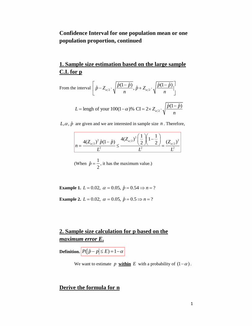
1. Sample size estimation based on the large sample

C.I. for p

From the interval 2 2

ˆ ˆ ˆ ˆ(1 ) (1 )ˆ ˆ,

p p p pp Z p Z

n n

2

ˆ ˆ(1 )lengh of your 100(1 )% CI 2

p pL Z

n

ˆ, ,L p are given and we are interested in sample size n . Therefore,

22 22

2 2

2 2 2

1 14( ) 1

ˆ ˆ4( ) (1 ) ( )2 2Z

Z p p Zn

L L L

(When 1

ˆ2

p , it has the maximum value.)

Example 1. ˆ0.02, 0.05, 0.54 ?L p n

Example 2. ˆ0.02, 0.05, 0.5 ?L p n

2. Sample size calculation for p based on the

maximum error E.

Definition. ˆ( ) 1P p p E

We want to estimate p within E with a probability of (1 ) .

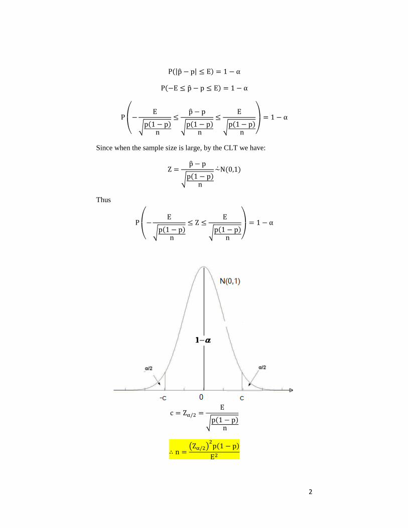
Derive the formula for n

2

(| | )

( )

(

√ ( )

√ ( )

√ ( ) )

Since when the sample size is large, by the CLT we have:

√ ( )

( )

Thus

(

√ ( )

√ ( ) )

√ ( )

( )

( )

3

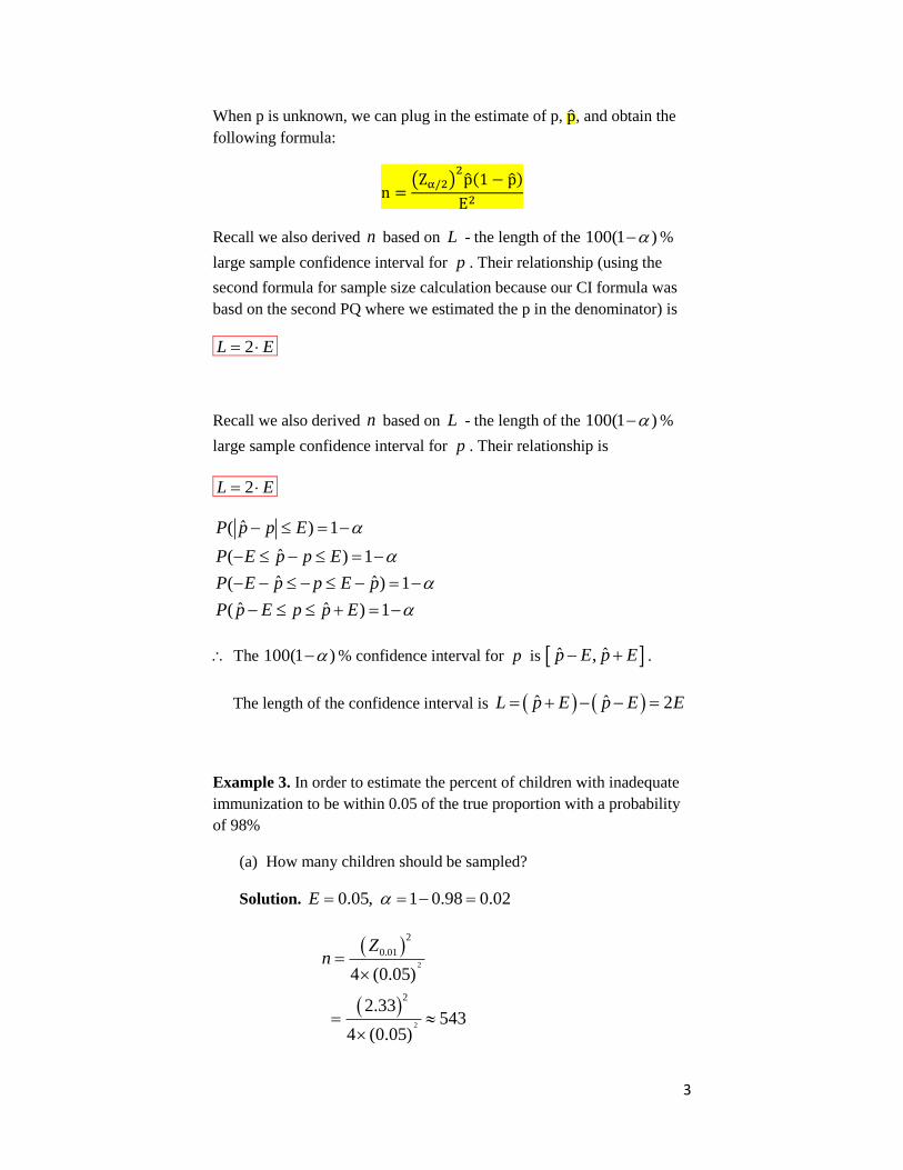
When p is unknown, we can plug in the estimate of p, , and obtain the

following formula:

( )

( )

Recall we also derived n based on L - the length of the 100(1 ) %

large sample confidence interval for p . Their relationship (using the

second formula for sample size calculation because our CI formula was

basd on the second PQ where we estimated the p in the denominator) is

2L E

Recall we also derived n based on L - the length of the 100(1 ) %

large sample confidence interval for p . Their relationship is

2L E

ˆ( ) 1

ˆ( ) 1

ˆ ˆ( ) 1

ˆ ˆ( ) 1

P p p E

P E p p E

P E p p E p

P p E p p E

The 100(1 ) % confidence interval for p is ˆ ˆ,p E p E .

The length of the confidence interval is ˆ ˆ 2L p E p E E

Example 3. In order to estimate the percent of children with inadequate

immunization to be within 0.05 of the true proportion with a probability

of 98%

(a) How many children should be sampled?

Solution. 0.05, 1 0.98 0.02E

2

2

2

0.01

2

4 (0.05)

2.33 543

4 (0.05)

Zn

4

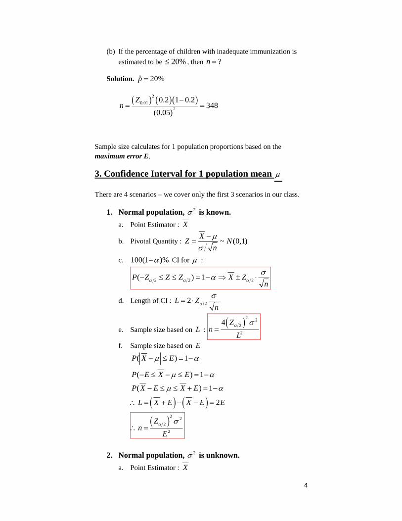
(b) If the percentage of children with inadequate immunization is

estimated to be 20% , then ?n

Solution. ˆ 20%p

2

2

0.01 0.2 1 0.2348

(0.05)

Zn

Sample size calculates for 1 population proportions based on the

maximum error E.

3. Confidence Interval for 1 population mean

There are 4 scenarios – we cover only the first 3 scenarios in our class.

1. Normal population, 2 is known.

a. Point Estimator : X

b. Pivotal Quantity : ~ (0,1)X

Z Nn

c. 100(1 )% CI for :

2 2 2( ) 1P Z Z Z X Zn

d. Length of CI : 22L Zn

e. Sample size based on L :

22

2

2

4 Zn

L

f. Sample size based on E

( ) 1P X E

( ) 1P E X E

( ) 1P X E X E

2L X E X E E

2

2

2

2

Zn

E

2. Normal population, 2 is unknown.

a. Point Estimator : X

5

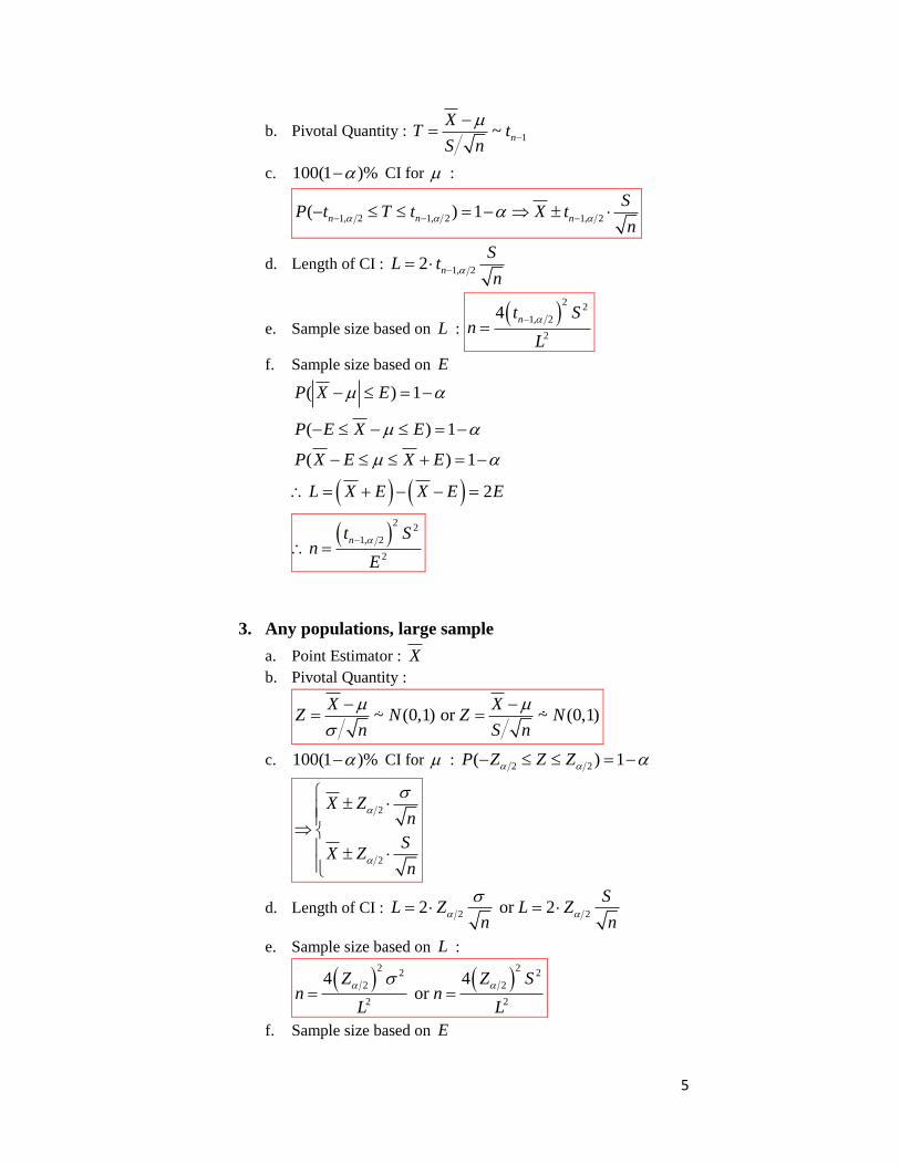
b. Pivotal Quantity : 1~ n

XT t

S n

c. 100(1 )% CI for :

1, 2 1, 2 1, 2( ) 1n n n

SP t T t X t

n

d. Length of CI : 1, 22 n

SL t

n

e. Sample size based on L :

22

1, 2

2

4 nt Sn

L

f. Sample size based on E

( ) 1P X E

( ) 1P E X E

( ) 1P X E X E

2L X E X E E

2

2

1, 2

2

nt Sn

E

3. Any populations, large sample

a. Point Estimator : X

b. Pivotal Quantity :

~ (0,1) or ~ (0,1)X X

Z N Z Nn S n

c. 100(1 )% CI for : 2 2( ) 1P Z Z Z

2

2

X Zn

SX Z

n

d. Length of CI : 2 22 or 2S

L Z L Zn n

e. Sample size based on L :

2 2

2 2

2 2

2 2

4 4 or

Z Z Sn n

L L

f. Sample size based on E

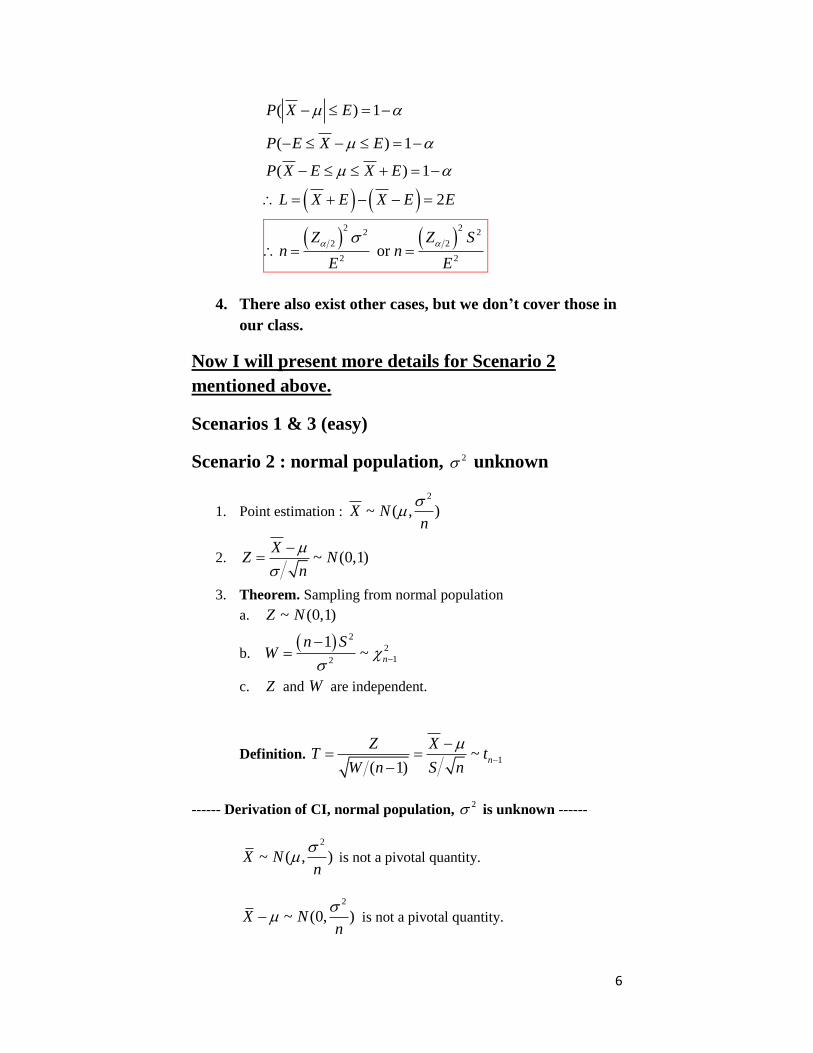
6

( ) 1P X E

( ) 1P E X E

( ) 1P X E X E

2L X E X E E

2 2

2 2

2 2

2 2 or

Z Z Sn n

E E

4. There also exist other cases, but we don’t cover those in

our class.

Now I will present more details for Scenario 2

mentioned above.

Scenarios 1 & 3 (easy)

Scenario 2 : normal population, 2 unknown

1. Point estimation :

2

~ ( , )X Nn

2. ~ (0,1)X

Z Nn

3. Theorem. Sampling from normal population

a. ~ (0,1)Z N

b. 2

2

12

1~ n

n SW

c. Z and W are independent.

Definition. 1~( 1)

n

Z XT t

W n S n

------ Derivation of CI, normal population, 2 is unknown ------

2

~ ( , )X Nn

is not a pivotal quantity.

2

~ (0, )X Nn

is not a pivotal quantity.

7

~ (0,1)/

XZ N

n

is not a pivotal quantity.

Remove !!!

Therefore 1~/

n

XT t

S n

is a pivotal quantity.

Now we will use this pivotal quantity to derive the 100(1-α)%

confidence interval for μ.

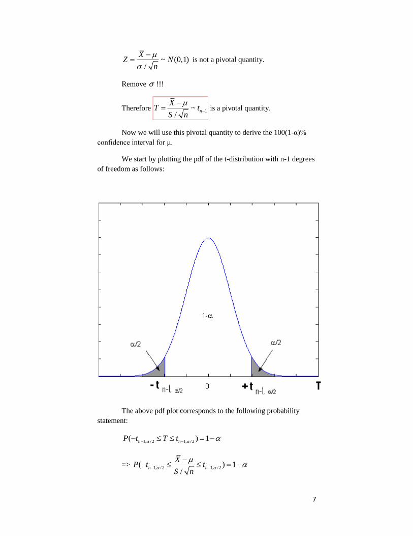
We start by plotting the pdf of the t-distribution with n-1 degrees

of freedom as follows:

The above pdf plot corresponds to the following probability

statement:

1, /2 1, /2( ) 1n nP t T t

=> 1, /2 1, /2( ) 1

/n n

XP t t

S n

8

=> 1, /2 1, /2( ) 1n n

S SP t X t

n n

=> 1, /2 1, /2( ) 1n n

S SP X t X t

n n

=> 1, /2 1, /2( ) 1n n

S SP X t X t

n n

=> 1, /2 1, /2( ) 1n n

S SP X t X t

n n

=> Thus the 100(1 )% C.I. for when 2 is unknown is

1, /2 1, /2[ , ]n n

S SX t X t

n n .

(*Please note that 1, /2 /2nt Z )

Example 4. In a random sample of 36n parochial schools throughout

the south, the average number of pupils per school is 379.2 with a

standard deviation of 124. Use the sample to construct a 95% CI for ,

the mean number of pupils per school for all parochial schools in the

south.

Solution. CI for , large sample

36, 379.2, 124, =0.05n X S

95% CI for is 0.05

124379.2 1.96

36

SX Z

n

338.7,419.7

Example 5. In a psychological depth-perception test, a random sample of

14n airline pilots were asked to judge the distance between 2 markers

at the other end of a laboratory.

The data (in test) are

9

2.7, 2.4, 1.9, 2.4, 1.9, 2.3, 2.2, 2.5, 2.3, 1.8, 2.5, 2.0, 2.2, 2.6

Please construct a 95% CI for , the average distance.

Solution.

(Note: we can perform the Shapiro-Wilk test to examine whether the

sample comes from a normal population or not. This test is not required

in our class. Here we simply assume the population is normal. I will

always give you such information in the exams.)

CI for , small sample, normal population, population variance

unknown.

14, 2.26, 0.28, =0.05n X S

95% CI for is 1, 2

0.282.26 2.16

14n

SX t

n

2.10,2.42

Example 6. A federal agency has decided to investigate the advertised

weight we printed on cartons of a certain brand of cereal. Historical data

show that 0.75 ounce. If we wish to estimate the weight within 0.25

ounce with 99% confidence, how many cartons should be sampled?

Solution. 0.25, 0.75, 0.01E

2 2

0.005

2

0.7560

0.25

Zn

Example 7. (review of exact CI for mean when the

population is normal and the population variance is

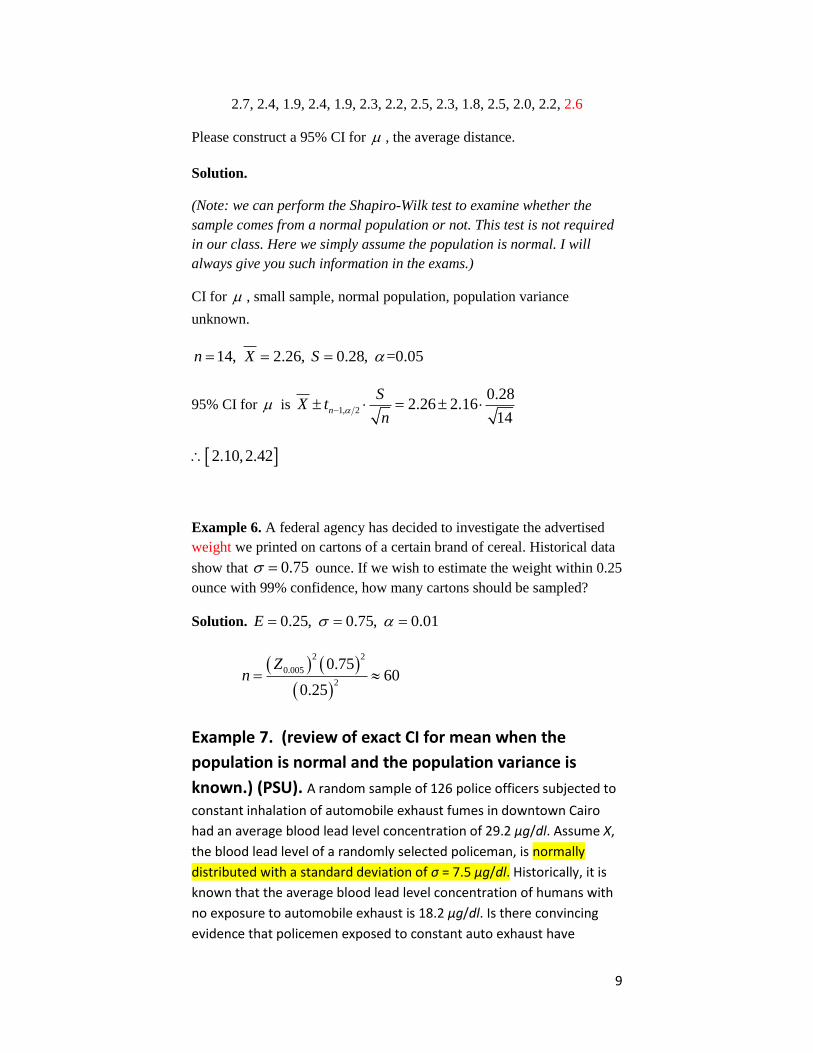
known.) (PSU). A random sample of 126 police officers subjected to

constant inhalation of automobile exhaust fumes in downtown Cairo

had an average blood lead level concentration of 29.2 μg/dl. Assume X,

the blood lead level of a randomly selected policeman, is normally

distributed with a standard deviation of σ = 7.5 μg/dl. Historically, it is

known that the average blood lead level concentration of humans with

no exposure to automobile exhaust is 18.2 μg/dl. Is there convincing

evidence that policemen exposed to constant auto exhaust have

10

elevated blood lead level concentrations? (Data source: Kamal,

Eldamaty, and Faris, "Blood lead level of Cairo traffic policemen,"

Science of the Total Environment, 105(1991): 165-170.)

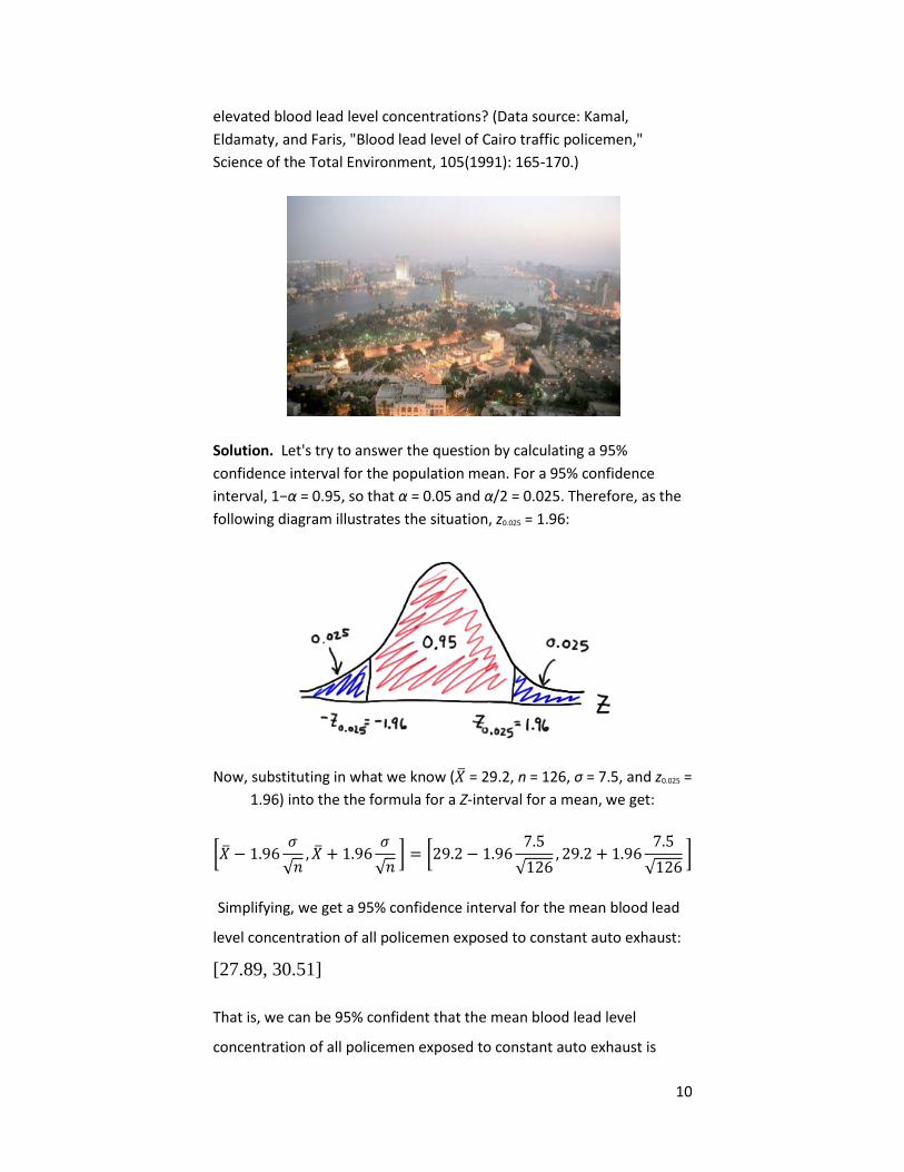
Solution. Let's try to answer the question by calculating a 95%

confidence interval for the population mean. For a 95% confidence

interval, 1−α = 0.95, so that α = 0.05 and α/2 = 0.025. Therefore, as the

following diagram illustrates the situation, z0.025 = 1.96:

Now, substituting in what we know ( = 29.2, n = 126, σ = 7.5, and z0.025 =

1.96) into the the formula for a Z-interval for a mean, we get:

[

√

√ ] [

√

√ ]

Simplifying, we get a 95% confidence interval for the mean blood lead

level concentration of all policemen exposed to constant auto exhaust:

[27.89, 30.51]

That is, we can be 95% confident that the mean blood lead level

concentration of all policemen exposed to constant auto exhaust is

11

between 27.9 μg/dl and 30.5 μg/dl. Note that the interval does not

contain the value 18.2, the average blood lead level concentration of

humans with no exposure to automobile exhaust. In fact, all of the

values in the confidence interval are much greater than 18.2. Therefore,

there is convincing evidence that policemen exposed to constant auto

exhaust have elevated blood lead level concentrations.

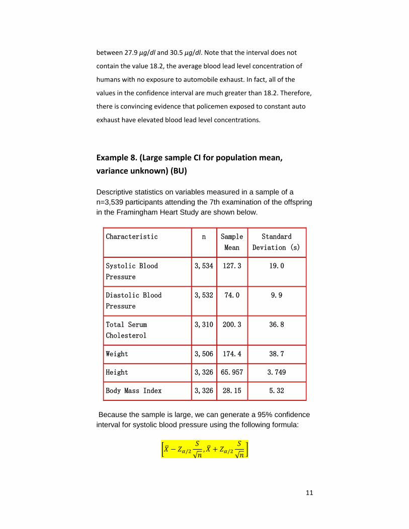
Example 8. (Large sample CI for population mean,

variance unknown) (BU)

Descriptive statistics on variables measured in a sample of a

n=3,539 participants attending the 7th examination of the offspring

in the Framingham Heart Study are shown below.

Characteristic n Sample

Mean

Standard

Deviation (s)

Systolic Blood

Pressure

3,534 127.3 19.0

Diastolic Blood

Pressure

3,532 74.0 9.9

Total Serum

Cholesterol

3,310 200.3 36.8

Weight 3,506 174.4 38.7

Height 3,326 65.957 3.749

Body Mass Index 3,326 28.15 5.32

Because the sample is large, we can generate a 95% confidence

interval for systolic blood pressure using the following formula:

[

√

√ ]

12

Substituting the sample statistics and the Z value for 95%

confidence, , we have

[

√

√ ] [ ]

Therefore, the point estimate for the true mean systolic blood

pressure in the population is 127.3, and we are 95% confident that

the true mean is between 126.7 and 127.9. The margin of error is

very small (the confidence interval is narrow), because the sample

size is large.

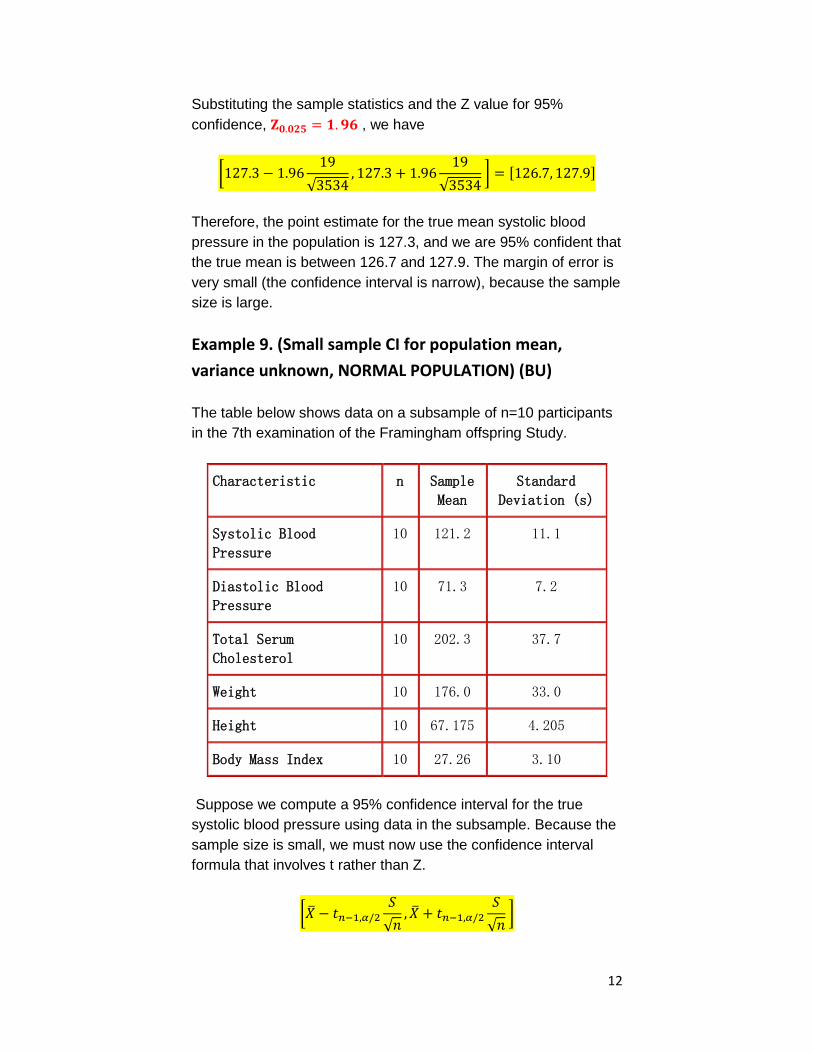
Example 9. (Small sample CI for population mean,

variance unknown, NORMAL POPULATION) (BU)

The table below shows data on a subsample of n=10 participants

in the 7th examination of the Framingham offspring Study.

Characteristic n Sample

Mean

Standard

Deviation (s)

Systolic Blood

Pressure

10 121.2 11.1

Diastolic Blood

Pressure

10 71.3 7.2

Total Serum

Cholesterol

10 202.3 37.7

Weight 10 176.0 33.0

Height 10 67.175 4.205

Body Mass Index 10 27.26 3.10

Suppose we compute a 95% confidence interval for the true

systolic blood pressure using data in the subsample. Because the

sample size is small, we must now use the confidence interval

formula that involves t rather than Z.

[

√

√ ]

13

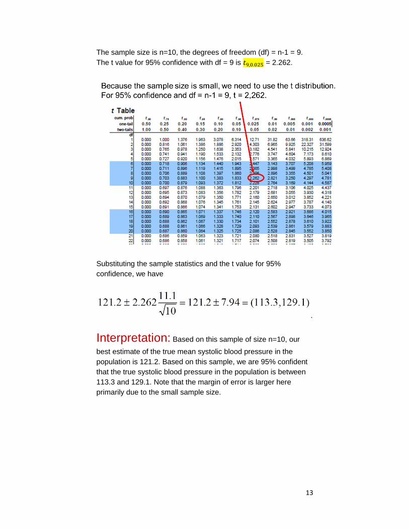
The sample size is n=10, the degrees of freedom (df) = n-1 = 9.

The t value for 95% confidence with df = 9 is = 2.262.

Substituting the sample statistics and the t value for 95%

confidence, we have

.

Interpretation: Based on this sample of size n=10, our

best estimate of the true mean systolic blood pressure in the

population is 121.2. Based on this sample, we are 95% confident

that the true systolic blood pressure in the population is between

113.3 and 129.1. Note that the margin of error is larger here

primarily due to the small sample size.