Exact Association Probabilityfor Data with Bias andFeatures

JAMES P. FERRY

A crucial prerequisite to data fusion is data association: i.e.,

the specification of which data arise from the same source. The

Bayesian approach to association pioneered by Mori and Chong is

based on principled probability formulas, which thus provide re-

liable confidence estimates for association hypotheses, in contrast

to approaches that rely on costs which can only be heuristically

transformed into probabilities. This paper extends the Bayesian ap-

proach in several ways. It presents a general derivation of associa-

tion probability between any number of sensors for arbitrary data

types, then derives specific results for kinematic and non-kinematic

cases. The kinematic case includes bias and is novel in three ways.

First, it is a proper Bayesian approach to bias which integrates

over all bias hypotheses rather than selecting one. Second, it han-

dles bias on an arbitrary number of sensors. Third, the formula

is exact: previous treatments of even the unbiased case involve an

integral approximation which is not needed here. The treatment of

features allows for several complex phenomena, including feature

behavior which depends on object type, and noisy and/or missing

feature data. A rigorous verification procedure is used to demon-

strate that the implementation of these formulas produces correct

probabilities.

Manuscript received December 04, 2008; revised August 20, 2009;released for publication December, 13, 2009.

Refereeing of this contribution was handled by Shozo Mori.

Authors’ address:Metron, Inc.,Reston,VA,E-mail: ferry@metsci.com.

1557-6418/10/$17.00 c° 2010 JAIF

1. INTRODUCTION

The data association problem arises whenever mul-tiple sensors are trained on a common region containingmultiple objects, which, in turn produce multiple mea-surements on each sensor. Having multiple views pro-vides more information about the state of the objects inthe region, provided the sensor data can be fused cor-rectly. In order to fuse the data, however, it is necessaryto know which measurements on different sensors arosefrom the same object. This is the data association prob-lem, and it is roughly forty years old [24, 25]. In manyapplications, these “measurements” are not raw sensormeasurements, but the posterior state estimates given bya single-sensor tracker such as a Kalman filter, and onespeaks of “measurement-to-track” or “track-to-track”associations. Solving the association problem is neces-sary in Multiple Hypothesis Tracking [23], and much ef-fort has gone into the development of algorithms to findthe best association given track estimates with Gaussianerror covariances [4]. The key difference between rawmeasurement data and track posteriors, however, is thatthe former lack inter-sensor correlation (for given objectstates). Such correlations are important in the track case,however, particularly if the posterior distributions havebeen influenced by previous inter-sensor data fusion.Indeed, even the posteriors of single-sensor trackers arecorrelated due to common process noise [3]. The scopeof this paper is limited to situations in which such inter-sensor correlations are absent or have been compensatedfor.

The association problem was originally formulatedin terms of costs with statistically motivated definitions–one found or devised a credible cost function andused it to seek low-cost associations. In 1990 Chong etal. introduced a more rigorous framework for assess-ing the quality of associations [7]. Mori and Chong ex-tended this work in a series of papers in the early 2000s[16, 17, 18, 19, 20]. For the important case of two sen-sors with Gaussian kinematic data, they replaced theheuristic framework of costs with a rigorous, Bayesianreformulation of the association problem. In doing so,they gave a meaningful definition of the probability ofan association, and argued that rather than seeking theassociation with minimal cost, one should seek the MAPassociation–i.e., the one with Maximal A posterioriProbability. In practice, the MAP method looks similarto the older method. The probabilities can be convertedto costs, and one ends up computing the same quantitiesas before with one subtle difference: Mori and Chongshowed that the correct cost threshold is not constant,but depends on the covariance matrices of the two mea-surements involved. Hence it came to be known as anadaptive threshold.

In 2002, Stone et al. generalized the work of Moriand Chong to non-kinematic data with the XMAP (eX-tended Maximal A posteriori Probability) method [27].In this and later work [6, 9, 11], association probabil-

JOURNAL OF ADVANCES IN INFORMATION FUSION VOL. 5, NO. 1 JUNE 2010 41

ity formulas have been derived that take into accountcontinuous and non-continuous data types beyond thepurely kinematic, primarily for the case of two sensors.

This paper encompasses and extends the previousXMAP work, beginning with a general derivation for as-sociation probability in an abstract setting in Section 2.Like [18], this derivation includes an arbitrary prior onthe number of objects and (in Appendix A) false alarms.Its novel aspects include a dependence on systematicerrors (such as bias or covariance inflation) and a cor-related prior on object state. In Section 3, this abstractderivation is applied to cases comprising kinematic andnon-kinematic data types, and the association probabil-ity formula is decomposed. The kinematic componentis dealt with in Section 4. The key contribution of thissection is its treatment of bias, which improves on pre-vious work in three ways: (1) rather than removing “thebias” (i.e., some particular bias hypothesis), it performsthe proper Bayesian operation of integrating over allbias hypotheses; (2) it holds for an arbitrary numberof sensors; and (3) it is exact–a certain integral ap-proximation typically made even in the non-bias case iscircumvented here. Section 5 demonstrates how to han-dle non-kinematic data in fairly complex cases, such aswhen the feature distributions and detection probabili-ties vary with object type. It also shows how to deal withmissing data, and provides a robust and general methodfor handling noisy features. Finally, Section 6 worksthrough an example in detail and demonstrates that themeaningful, exact probabilities produced by XMAP canbe used to verify the formulas and their implementationto high precision.

2. ASSOCIATION PROBABILITY DERIVATION

This section derives a general formula for associ-ation probability in an abstract space. Working in anabstract space allows us to handle arbitrary types ofmeasurement data in a consistent manner, whether itbe traditional kinematic data, or, say, the messy outputof a feature extractor which combines real-valued datawith object classification calls and status flags. Thus,the bulk of this paper may be viewed as applying thegeneral Theorem 2.4 below to special cases. A technicaldetail to bear in mind with this abstract treatment is thatintegrating over an abstract space requires one to specifya measure over the space. There will be no need, in thispaper, to use measures other than Lebesgue measure forcontinuous data and counting measure for discrete data(which converts integrals to sums), so we will assumethat the measure is clear from context.

We begin with a simple result for the probabilitydensity of getting a specific array of measurements ona single sensor s given the states of the objects thatproduced them. This result depends on the measure-ment likelihood function Ls(z j x,¯), which specifies theprobability density of the measurement z arising giventhat the object which produced it was detected and was

in state x, and that a systematic error ¯ is acting on allmeasurements on sensor s. It depends also on the de-tection probability PsD(x) for an object in state x, and weuse the notation QsD(x) = 1¡PsD(x) to denote the non-detection probability. This systematic error ¯ may rep-resent any measurement error process that acts on allmeasurements on a sensor at once, such as a transla-tional bias or covariance inflation.

Let zs = (zsi )ns

i=1 denote an array of the ns measure-ments on sensor s at some fixed time, and x= (xj)

nj=1

denote the array of states of the n objects in scene. Welet J = f1,2, : : : ,ng denote the set of all objects, and JsDdenote the subset of objects detected on sensor s. Weuse the mapping as : JsD!f1,2, : : : ,nsg to specify whichobject produced which measurement. We assume thereare no false alarms (the false-alarm case is addressed inAppendix A), that there are no split or merged measure-ments, and that all permutations of measurement labelsare equally likely. With these assumptions, we obtainthe following preliminary result.

LEMMA 2.1 The probability density of the measurementarray zs arising according to the mapping as given theobject state array x and the systematic error ¯s is

Pr(zs,as j x,¯s) = 1ns!

Yj2JsD

PsD(xj)Ls(zsas(j) j xj ,¯s)

£Yj2JnJsD

QsD(xj): (2.1)

PROOF Given the object state array x, the probabilityPr(JsD j x) of the subset of detected objects being pre-cisely JsD is the product of PsD(xj) over j 2 JsD timesthe product of QsD(xj) over j 2 JnJsD. Given JsD (andx), each of the possible ns! mappings as are equallylikely, so Pr(as,JsD j x), which is identical to Pr(as j x)because as determines JsD, can be expressed Pr(as j x) =Pr(as j JsD,x)Pr(JsD j x) = Pr(JsD j x)=ns!. The probabilitydensity of the measurement array zs given as, x, and¯s is the product of the individual likelihood functionsLs(zsi j xj ,¯s), where i= as(j), over all j 2 JsD. Equa-tion (2.1) now follows from Pr(zs,as j x,¯s) = Pr(zs jas,x,¯s)Pr(as j x).

It is straightforward to generalize Lemma 2.1 froma single sensor to a set of sensors S. We let z= (zs)s2Sdenote the array of all individual measurement arrays zs,and ¯ = (¯s)s2S denote the array of all systematic errors.We assume that the measurement process is independentbetween sensors, bearing in mind that this limits theapplicability to tracking unless the inter-sensor depen-dence can be compensated for. With multiple sensorsit is convenient to express the information contained inthe mappings fasgs2S in terms of

a(j) = f(s, i) : as(j) = ig and a(j) = fs : j 2 JsDg:(2.2)

42 JOURNAL OF ADVANCES IN INFORMATION FUSION VOL. 5, NO. 1 JUNE 2010

The function a gives the set of sensors which detecteach object j, whereas a gives the measurement indicesof each detection too. With this notation, we have thefollowing corollary of Lemma 2.1.

COROLLARY 2.2 The probability density of the measure-ment arrays z arising according to the function a giventhe object state array x and the systematic errors ¯ is

Pr(z,a j x,¯) =ÃY

s2S

1ns!

!Yj2J

£Ã Y

(s,i)2a(j)PsD(xj)L

s(zsi j xj ,¯s)Ys=2a(j)

QsD(xj)

!:

(2.3)

PROOF The assumption of independence between themeasurement processes implies that Pr(z,a j x,¯) maybe obtained as the product of (2.1) over s 2 S. The result(2.3) is merely a rearrangement of this.

We now seek to eliminate the dependence on thestate array x. To do so, we need an expression for theprior distribution of the state. The expression introducedbelow is novel, and requires some discussion of (a) theshortcomings of the usual approach, (b) how the prob-lem should be solved in principle, and (c) the compro-mise used here. Although the derivation in this sectionapplies to an arbitrary state space, the problematic caseis the traditional, kinematic one, so we shall think of xas a kinematic quantity for this discussion.

The usual assumption about the prior distribution ofx when bias is absent is that its components xj are i.i.d.,each distributed according to some known distributionp0. The distribution p0(x) of a single object state x isthen taken to be uniform over some finite region ofspace X0 [17]. An appropriate volume V for X0 may beestimated from the data, and p0(x) modeled as IX0 (x)=V,where IX0 (x) is the indicator function for the region X0.The precise location of the region X0 does not matterbecause p0(x) is later approximated by the constant 1=Vin the integrals where it appears. This approximationis valid because the measurement errors are typicallymuch smaller than X0, and this formulation, which leadsto the adaptive threshold works well in practice [26].

Bias errors may be larger than X0, however, so theapproximation p0(x)¼ 1=V fails in the bias case. Main-taining p0(x) as IX0 (x)=V yields intractable integrals, soit is natural to consider a Gaussian model for p0(x). Inthis case, however, the precise location of the Gaussian’speak in state space must be estimated from the measure-ments, while correcting for the (unknown) biases, andthe resulting formulation becomes messy and ad hoc.Indeed, it must be ad hoc because it involves estimatingthe location of the Gaussian’s peak from the data–aclear violation of Bayesian methodology.

One is led to such violations because of a faulty ini-tial assumption: that the prior distribution of x is well

modeled as the product of p0(xj) for some known distri-bution p0. The characteristic size V and nominal center» of this prior distribution are usually both unknown.However, it is reasonable to model the states xj as beingconditionally i.i.d. given V and », and then to specifypriors on V and ». This leads to additional integrals overV and ». However, one may argue, for example, that theweight in the integrand of the integral over V is con-centrated in the region of V-space that is reinforced bythe measurement data, so evaluating the integrand at asingle point V¤ (estimated from the data) amounts to areasonable approximation of the integral. This providesa Bayesian justification for an otherwise ad hoc proce-dure. However, in the bias case there is no single valueof » where the integrand is concentrated: this center lo-cation depends on the unknown biases ¯s. Rather thanreplace » by this function of the biases, it is fairly easyto retain it and perform the integrals exactly. Doing thesame for V, however, (which, in the Gaussian case is ac-tually an entire covariance matrix) is too difficult, so wewill estimate it from the data, relying on the argumentabove for justification.

We therefore assume the following prior distributionon the state array x (which we now resume treating asabstract rather than kinematic):

p0(x j n,») =Yj2Jp0(xj j »): (2.4)

Multiplying (2.3) by p0(x j n,») and integrating over xresults in a product of integrals over xj for each objectj 2 J . These have the form

P®(z j ¯,») =Zp0(x j »)

Y(s,i)2®

PsD(x)Ls(zsi j x,¯s)

£Ys=2®QsD(x)dx (2.5)

for ®= a(j). For the special case of ® containing onlythe single measurement (s, i) we will use the notationPs(zsi j ¯,») in lieu of P®(z j ¯,»). Let JD denote thesubset of objects in J detected on some sensor, andnD = jJDj be the number of detected objects. For j =2 JD,(2.5) takes a particularly simple form:

q=Zp0(x j »)

Ys2SQsD(x)dx: (2.6)

Here we are imposing the condition that q is indepen-dent of ». This will happen automatically later whenwe stipulate in (3.18) that PsD(x) be independent of thekinematic component of x. This stipulation is not realis-tic: PsD(x) can vary greatly with aspect angle and range.However, the case in which PsD(x) has kinematic depen-dence makes the calculations in Section 4 too compli-cated, though it would be a suitable topic for futurework.

COROLLARY 2.3 The probability density of the measure-ment arrays z arising according to the function a given

EXACT ASSOCIATION PROBABILITY FOR DATA WITH BIAS AND FEATURES 43

the number of objects n, the systematic errors ¯, and thecenter » of the prior region of state space is

Pr(z,a j n,¯,») = qn¡nDQs2S ns!

Yj2JD

Pa(j)(z j ¯,»): (2.7)

PROOF This is obtained by multiplying (2.3) by (2.4)and integrating over x.

The function a defined in (2.2) maps each object tothe set of measurements it produces. An association [a]is defined to be the collection of these sets, [a] = fa(j) :j 2 JDg. There are exactly n!=(n¡nD)! functions a0 forwhich [a0] = [a], all of which are equally probable, sothe association probability Pr(z, [a] j n,¯,») is n!=(n¡nD)! times Pr(z,a j n,¯,»). We may now eliminate thedependence on the total number of objects n. The priorprobability for the number of objects being n is denoted½0(n), so

Pr(z, [a] j ¯,») = °0(nD)Qs2S ns!

Y®2[a]

P®(z j ¯,»), (2.8)

where

°0(nD) =1Xn=nD

½0(n)n!

(n¡nD)!qn¡nD : (2.9)

We denote the prior on the systematic errors P0(¯),and the prior on the center, P0

¥ (»). When integrating(2.8), the key quantity to compute is

F(z, [a]) =Z Z Y

®2[a]P®(z j ¯,»)P0(¯)P0

¥ (»)d¯d»:

(2.10)

Finally, we introduce the following ratios of °0 and Fto their values for the null association a0, which assignseach of the nT measurements in z to a distinct object:

g([a]) =°0(nD)°0(nT)

and G(z, [a]) =F(z, [a])F(z, [a0])

:

(2.11)

THEOREM 2.4 The probability of the association [a]given the measurements z is

Pr([a] j z) = Pr([a0] j z)g([a])G(z, [a]): (2.12)

PROOF From (2.8) we observe that joint probabil-ity density Pr(z, [a]) is F(z, [a]) times °0(nD) dividedby the product of the ns!. The conditional probabilityPr([a] j z) of an association given the measurement datais Pr(z, [a])=Pr(z). Dividing Pr([a] j z) by the normaliza-tion constant Pr([a0] j z) yields (2.12).

The key to computing the association probability isevaluating F(z, [a]) (or its normalization G(z, [a])). Thisis the topic of Sections 3—5. The combinatorial factorg([a]) encapsulates the effect of the prior distributionof the number of objects. Formulas for it are given in

Appendix B. Although the derivation in this section as-sumed there are no false alarms, Appendix A demon-strates that the effect of false alarms may be included bymodifying the factor g([a])–no change to the definitionof G(z, [a]) is necessary.

3. SIMPLIFICATION FOR SPECIAL CASES

Theorem 2.4 gives a general formula for associationprobability, but requires the evaluation of the integralsin (2.5) and (2.10). With complicated data types, eval-uating these integrals is not as simple as it may appear.Therefore we demonstrate how the problem simplifiesin various special cases. Section 3.1 gives a formulamuch simpler than (2.12) which holds when there isno dependence on ¯ or ». Section 3.1.1 specializes thisfurther to the two-sensor, kinematic case, connectingthe general XMAP formulation presented here to theoriginal MAP formulation of Mori and Chong [16, 17].Finally, Section 3.2 demonstrates how to decompose theproblem into kinematic and non-kinematic componentswhen both data types are present. The kinematic com-ponent is then evaluated explicitly in Section 4, and thenon-kinematic component in Section 5.

3.1. Simplification in the Absence of Systematic Error

When the systematic errors ¯ and the center » areknown, we may assume each to be zero (by suitablytransforming the data z): i.e., P0(¯) = ±(¯), and P0

¥ (») =±(»). Letting P®(z) and Ps(zsi ) denote P®(z j 0,0) andPs(zsi j 0,0), respectively, we define

R®(z) =P®(z)Q

(s,i)2®Ps(zsi ), (3.1)

which is the ratio of the probability density of themeasurements in ® arising from a single object to theprobability density that each arises from a differentobject (aside from a factor which accounts for thedifferent number of detected objects in the two cases–this is embedded in g([a])).

THEOREM 3.1 When the systematic errors ¯ and thecenter » are known, the probability of the association [a]given the measurements z is

Pr([a] j z) = Pr([a0] j z)g([a])Y®2[a]+

R®(z), (3.2)

where [a]+ denotes the subset of those ® 2 [a] with atleast two measurements.

PROOF Because R®(z) = 1 when j®j= 1, the productover ® 2 [a]+ in (3.2) may be extended to ® 2 [a]. Thisproduct equals F(z, [a])=F(z, [a0]) when we set P0(¯) =±(¯) and P0

¥ (») = ±(») in (2.10).

3.1.1. Two-sensor kinematic caseTo recover the original MAP result [16, 17], we be-

gin with Theorem 3.1 and make four further simplify-

44 JOURNAL OF ADVANCES IN INFORMATION FUSION VOL. 5, NO. 1 JUNE 2010

ing assumptions: first, that ½0(n) is Poisson distributed;second, that there are only two sensors; third, that thedetection probabilities on each sensor are constant; andfourth, that the data is purely kinematic, with Gaussianmeasurement error distributions. The two-sensor kine-matic case without bias is important because it admits acomputationally efficient solution. One first constructsa cost matrix whose entries cij are the Mahalanobis dis-tances between measurement i on sensor 1 and measure-ment j on sensor 2. Then a cost threshold is subtractedfrom each cij . Finally, one finds the association withminimal total cost using, for example, the JVC algo-rithm [8, 13], and, if desired, iterates this process usingMurty’s algorithm [21] to get the k best associations.(When there are more than two sensors, however, find-ing the association with least cost is known to be NP-hard. Approximate methods have been employed basedon Lagrangian relaxation [22] or on stitching togethersolutions to pairwise problems. These approaches arecompared in [2].)

The effect of letting ½0(n) be Poisson distributed isdiscussed in Appendix B. It allows us to replace (3.2)with the purely multiplicative form (B.4). Specializingto two sensors simplifies matters further because in thiscase every ® 2 [a]+ has the form ®= f(1, i), (2,j)g. Wemay re-write this more compactly as ®= (i,j). Thus thetwo-sensor version of (B.4) may be written

Pr([a] j z) = Pr([a0] j z)Y

(i,j)2[a]+Rij(z), (3.3)

where

Rij(z) =P12(z1i ,z

2j )

P1(z1i )P2(z2j )

: (3.4)

The functions Ps and P12 are special cases of (2.5), with¯ and » eliminated, PsD set to a constant, and factors ofº in (B.5) included:

Ps(zsi ) = ºPsDQ

3¡sD

Zp0(x)Ls(zsi j x)dx and

(3.5)

P12(z1i ,z2j ) = ºP

1DP

2D

Zp0(x)L1(z1i j x)L2(z2j j x)dx:

(3.6)

(To incorporate false alarms, replace the factor ºPsDQ3¡sD

in (3.5) with ºPsDQ3¡sD + ºsFA, where º

sFA is the expected

number of false alarms on sensor s: see (B.18).)The integrals in (3.5) and (3.6) are simple to evaluate

when Ls has a Gaussian distribution. We use the notation

N (x;¹,V) =1pj2¼Vj exp

�¡12(x¡¹)TV¡1(x¡¹)

¶

(3.7)

for a Gaussian in x with mean ¹ and covariance matrixV. Specializing to the standard kinematic case, we letthe value zsi of measurement i on sensor s have the form

zsi = (ysi ,Vsi ), where y

si the state estimate, and Vsi is the

error estimate on ysi . We then stipulate that

Ls(zsi j x) =N (ysi ;x,Vsi )PV(V

si ): (3.8)

Essentially this means that ysi has a Gaussian distributioncentered at the true state x, with covariance matrix givenby Vsi . There is an additional complication, however: theestimated covariance matrix Vsi is part of the data, so itsdistribution must be modeled as well. The simplest as-sumption is that it is independent of x (and of ysi ). Inthis case the precise form of the distribution PV does notmatter: it drops out of the calculation. (More sophis-ticated treatments are certainly possible: for example,there may be systematic over- or under-reporting of co-variance, or the size of the covariance matrix itself mayyield object-type information, in which case PV wouldbe modeled to have a dependence on the object typecomponent of the state.)

Following [7], we let the prior distribution on anobject’s state x be constant over some region X0:

p0(x) =1

Vol(X0)IX0 (x), (3.9)

where IX0 (x) is equal to 1 for x 2 X0, and 0 otherwise.Given the above assumptions, (3.4) may be written

Rij(z) =N (y1i ;y2j ,V

1i +V2

j )Vol(X0)ºq

£RX0N (x;¹ij ,Wij)dxR

X0N (x;y1i ,V1i )dx

RX0N (x;y2j ,V

2j )dx

,

(3.10)

where q=Q1DQ

2D, and ¹ij and Wij are given by

¹ij = y1i +V

1i (V

1i +V2

j )¡1(y2j ¡ y1i ) and

Wij = V1i (V

1i +V2

j )¡1V2

j :(3.11)

Assuming the Gaussians in the integrals in (3.10) havemost of their weight within X0, each integral is approx-imately 1. This yields the following cost of associatingi and j:

cij =¡2log Rij(z)= (y1i ¡ y2j )T(V1

i +V2j )¡1(y1i ¡ y2j )¡Aij ,

(3.12)where

Aij = 2logVol(X0)¡ log j2¼(V1i +V2

j )j ¡ 2log(ºq):

(3.13)

The cost cij is thus seen to be the Mahalanobis dis-tance (y1i ¡ y2j )T(V1

i +V2j )¡1(y1i ¡ y2j ) between the mea-

surement pair (i,j) minus Mori and Chong’s adaptivethreshold Aij [16, 17, 18]. Traditionally, a variety ofmethods had been used to set this threshold [4, 5].Although the main historical significance of Mori andChong’s work is the introduction of a rigorous Bayesian

EXACT ASSOCIATION PROBABILITY FOR DATA WITH BIAS AND FEATURES 45

approach to association, the more immediate impactwas the introduction of a threshold Aij which has beenshown to be superior to the previous, fixed thresholds[26].

There is a minor flaw with (3.13), however: it failswhen some Vsi are large relative to the region X0 becausethis violates the assumption that allowed the integralsin (3.10) to be approximated as 1. Such measurementsmust be preprocessed out as unassociatable when using(3.13). Additional, non-kinematic data may render suchmeasurements associatable, however, so it is preferableto modify (3.13) to be robust to any input Vsi . A com-plicated method for doing this is given in [9], but here amuch simpler method is given. When the covariance of aGaussian being integrated is large compared to X0, theintegral may be approximated as the Gaussian’s peakvalue times Vol(X0). This leads to the following robustmodification of (3.13), which has the heuristic interpre-tation of limiting the uncertainty of an object’s locationto X0 even if Vsi !1:

Aij =max(2logVol(X0)¡ log j2¼(V1i +V2

j )j,0)¡ 2log(ºq): (3.14)

To use the adaptive threshold (3.14) one needs val-ues for q, º, and Vol(X0). Section 2 notes that whensuch parameters are unknown, the proper Bayesian pro-cedure is to give them a prior distribution and inte-grate them out of the problem. In practice, however,setting values of PsD that are even approximately cor-rect produces better results than those obtained usingthe traditional, fixed threshold [26]. These values areused to compute q= (1¡P1

D )(1¡P2D ) and, using (B.6),

º = (n1 + n2)=(P1D +P2

D ).It remains to estimate Vol(X0). Following [9], we

do this by first estimating the covariance of the locationdata ysi for all measurements. In the absence of sensorbias, the unbiased covariance estimator V may be com-puted as follows. Collect all nT measurement positionsysi on all sensors into a single array with elements yi fori= 1,2, : : : ,nT. Then

V =1

nT ¡ 1

nTXi=1

(yi¡ y)(yi¡ y)T where y =1nT

nTXi=1

yi:

(3.15)

In Section 4 we will consider the case with r sensorsand bias. In this case, V is given by

V =1

nT¡ rXs2S

nsXi=1

(ysi ¡ ys)(ysi ¡ ys)T where

(3.16)

ys =1ns

nsXi=1

ysi :

To compute the volume of X0 from V, we assumethat X0 is a Cartesian product of ellipsoidal regions

with covariance matrix V. If X0 is a product of m-dimensional ellipsoids (e.g., x could be 6-dimensional,with m= 3 being the physical dimension of position-and of velocity-space), then

Vol(X0) =qj2¼�Vj where � = (1+m=2)(m=2)!¡2=m:

(3.17)

The values of � for m= 1, 2, and 3 are 6=¼ ¼ 1:91,2, and (5=3) 3

p6=¼ ¼ 2:07, respectively. Because these

values are so close, setting � = 2 for all problems is anacceptable approximation.

This volume estimate is not ideal. It is sensitive tooutliers and to measurements being close to co-planar.Fortunately, its effect is limited to the threshold–i.e.,the decision of whether to associate two measurementsat all. Some authors dispense with the volume estima-tion entirely, using a diffuse spatial prior [14, 15], whichis perfectly valid, but limits the power of the resultingmethod to hypothesis tests between associations repre-senting the same number of detected objects.

3.2. Splitting into Components

When z comprises various data types, with some de-gree of independence in how each type is generated,(2.12) can be split into components for each data type.Here we will make a major simplification by splittingthe kinematic data from any non-kinematic data typespresent. The kinematic data retain the complications dueto ¯ and », and Section 4 demonstrates how to handlethis. The non-kinematic data is modeled to be withoutthe complications due to ¯ and »: therefore the non-kinematic component of association probability simpli-fies into a product over ® 2 [a]+, as in Theorem 3.1.Examples of how to model various non-kinematic datatypes are given in Section 5.

To split the problem into components, we split boththe state x and each measurement zsi into a kinematiccomponent (K) and another component (J , for all non-kinematic variables jointly): let x= (xK ,xJ ) and zsi =(zKsi ,zJsi ). We make the following assumptions abouthow the prior distribution, detection probability, andmeasurement likelihood functions split:

PsD(x) = PJsD (xJ ), (3.18)

p0(x j ») = pK0(xK ¡ »)pJ0(xJ ) and

(3.19)

Ls(zsi j x,¯s) = LKs(zKsi j xK ,¯s)LJs(zJsi j xJ ):(3.20)

Equation (3.18) stipulates that the detection probabilityis independent of the kinematic state. As discussed inSection 2, this is an unfortunate but necessary oversim-plification. It is allowed to depend on non-kinematicvariables, however: for example, it is plausible that onecould have a reasonable model of detection probability

46 JOURNAL OF ADVANCES IN INFORMATION FUSION VOL. 5, NO. 1 JUNE 2010

as a function of object type (cf. Section 5.1). Equations(3.19) and (3.20) stipulate that the complications due tothe center » of the object region and the systematic error¯s are solely kinematic phenomena. The assumptions(3.18)—(3.20) permit a relatively simple treatment of thenon-kinematic variables, while addressing the effects ofkinematic bias.

The definition of q in (2.6) may be simplified to

q=Z Y

s2SQJsD (xJ )dxJ , (3.21)

because for any » the integral of pK0(xK ¡ ») over allxK is 1. Note that q is independent of », as requiredin the text following (2.6). The key probability densityP®(z j ¯,») may be split as follows:

P®(z j ¯,») = PK®(zK j ¯,»)PJ®(zJ ), (3.22)

using (2.5) to give us these formulas for the kinematicand non-kinematic components of P®:

PK®(zK j ¯,») =ZpK0(xK ¡ »)

Y(s,i)2®

LKs(zKsi j xK ,¯s)dxK and

(3.23)

PJ®(zJ ) =ZpJ0(xJ )

Y(s,i)2®

PJsD (xJ )LJs(zJsi j xJ )

£Ys=2®QJsD (x

J )dxJ : (3.24)

THEOREM 3.2 Given the assumptions (3:18)—(3:20), theprobability of the association [a] given the measurementsz is

Pr([a] j z) = Pr([a0] j z)g([a])GK(zK , [a])GJ (zJ , [a]),(3.25)

with

GK(zK , [a]) =FK(zK , [a])FK(zK , [a0])

, (3.26)

where

FK(zK , [a]) =Z Z Y

®2[a]PK®(zK j ¯,»)P0(¯)P0

¥ (»)d¯d»,

(3.27)

andGJ (zJ , [a]) =

Y®2[a]+

RJ®(zJ ), (3.28)

where

RJ®(zJ ) =PJ®(zJ )Q

(s,i)2®PJs(zJsi ): (3.29)

PROOF This result follows directly from the definitionsof the quantities involved.

4. THE KINEMATIC COMPONENT

In this section we derive an exact formula for thekinematic component GK(zK , [a]) of the association

probability in the case of an arbitrary number of sensorswith bias effects included. We will drop the superscriptK throughout this section. Equation (3.26) shows thatevaluating G(z, [a]) involves integrating over the sen-sor biases ¯. This differs from the more typical ap-proaches which identify and remove a bias hypothe-sis (either a distinct hypothesis for each association, or,more crudely, one hypothesis for all associations). Suchapproaches can fail even in quite simple scenarios, suchas the one discussed in [10].

To obtain a formula for the kinematic componentG(z, [a]) of the association probability, we must evaluatethe integrals in (3.23) and (3.27). To do so, we needappropriate models for the quantities which appear inthem. For the bias prior we assume

P0(¯) =Ys2SP0s(¯s) =

Ys2SN (¯s;¯s0,B

s): (4.1)

Here ¯s0 is the mean bias on sensor s, and Bs is thebias covariance matrix. In practice, one would typicallyset ¯s0 to zero because one could simply add it toeach measurement on sensor s in a pre-processing step.The bias covariance matrix Bs should be part of theperformance specifications for sensor s. If it is not,however, one may set Bs to be diffuse. We let the prioron » be diffuse:

P0¥ (») =N (»;»0,V¥) where V¥ !1: (4.2)

The irrelevant value of »0 will be retained until the stepthat takes V¥ !1 eliminates it.

We let the measurement likelihood function beGaussian, writing the measurement as zsi = (ysi ,V

si ), as

in Section 3.1.1. Generalizing (3.8) to include bias, wehave

Ls(zsi j x,¯s) =N (ysi ;x¡¯s,Vsi ): (4.3)

Here the factor PV(Vsi ) which appeared in (3.8) has been

set to 1 (because the value does not matter, and it would,in fact, be 1 in a suitably chosen measure space). Finally,we assume that the prior distribution on x is Gaussianwith mean » and known variance V0,

p0(x¡ ») =N (x;»,V0), (4.4)

for the reasons discussed before Equation (2.4). Equa-tion (3.16) may be used to produce a value for V0 inpractice.

LEMMA 4.1

P®(z j ¯,») =pj2¼W®jN (»,¹®,V0)

Y(s,i)2®

N (ysi +¯s;¹®,V

si ),

(4.5)where

W® =

0@V¡10 +

X(s,i)2®

(Vsi )¡1

1A¡1

and

¹® =W®

0@V¡10 »+

X(s,i)2®

(Vsi )¡1(ysi +¯

s)

1A :

(4.6)

EXACT ASSOCIATION PROBABILITY FOR DATA WITH BIAS AND FEATURES 47

PROOF With (4.1)—(4.4), the integrand in (3.23) be-comes a product of Gaussians, which may be integratedusing the standard formula (D.3).

Substituting (4.5) into (3.27) produces the followingkey integral to evaluate:

F(z, [a]) =

ÃY®2[a]

pj2¼W®j

!Z Z¢ ¢ ¢

£Z Y

®2[a]

ÃN (»,¹®,V0)

Y(s,i)2®

N (ysi +¯s;¹®,V

si )

!

£Ys2SN (¯s;¯s0,B

s)N (»;»0,V¥)d¯1d¯2 ¢ ¢ ¢d¯rd»:

(4.7)Evaluating (4.7) yields the kinematic componentG(z, [a]) of the association probability Pr([a] j z) in(3.25). Two formulas for G(z, [a]) will be given. First,Theorem 4.2 provides a formula based on the directevaluation of (4.7). Theorem 4.3 then gives a more com-putationally efficient formula achieved by applying cer-tain transformations to the first result.

THEOREM 4.2

G(z, [a]) = C exp

á12

÷([a]) +

X®2[a]

·®

!!,

(4.8)

where C is chosen so that G(z, [a0]) = 1, and the costs·([a]) and ·® are defined by

·([a]) = log jUj ¡bTU¡1b, and (4.9)

·® = log jV0W¡1® j ¡mT®W¡1

® m®: (4.10)

The matrix U and vector b have the following blockstructure:

U=

0BBBBBBB@

U1,1 U1,2 ¢ ¢ ¢ U1,r U1,0/

U2,1 U2,2 ¢ ¢ ¢ U2,r U2,0/

......

. . ....

...

Ur,1 Ur,2 ¢ ¢ ¢ Ur,r Ur,0/

U0/,1 U0/,2 ¢ ¢ ¢ U0/,r U0/,0/

1CCCCCCCA

and b=

0BBBBBBB@

b1

b2

...

br

b0/

1CCCCCCCA:

(4.11)The entries in U are matrices defined as follows. Fors1,s2 2 S,

Us1,s2 = ±s1s2Us1 ¡

X®2[a]

Is1® Is2® (V

s1¶s1®)¡1W®(V

s2¶s2®)¡1,

(4.12)

Us1,0/ =¡X®2[a]

Is1® (Vs1¶s1®)¡1W®V

¡10 ,

(4.13)U0/,s2 =¡

X®2[a]

Is2® V¡10 W®(V

s2¶s2®)¡1,

U0/,0/ = nDV¡10 ¡

X®2[a]

V¡10 W®V¡10 , (4.14)

where Is® = 1 if s 2 ® (and ¶s® denotes the (unique) i forwhich (s, i) 2 ® in this case), and Is® = 0 when s =2 ®.Similarly, for s 2 S, the entries in b are vectors definedby

bs = (Bs)¡1¯s0¡X®2[a]

Is®(Vs¶s®)¡1(ys¶s® ¡m®) and

(4.16)b0/ = V

¡10

X®2[a]

m®:

The components of U and b depend on the followingquantities:

W® =

0@V¡10 +

X(s,i)2®

(Vsi )¡1

1A¡1

,

(4.17)

m® =W®X(s,i)2®

(Vsi )¡1ysi and

Us = (Bs)¡1 +nsXi=1

(Vsi )¡1: (4.18)

PROOF Equation (4.7) is more complicated than it ap-pears: the notation ¹®, defined in (4.6), conceals a de-pendence on each of the integration variables in manyof the Gaussian factors. Nevertheless, (4.7) is just an in-tegral of products of Gaussians, where the arguments ofthe Gaussians are linear combinations of the integrationvariables. Equation (D.10) provides a formula for inte-grals of this form. To use this formula, we first must ex-plicitly cast (4.7) in the form of (D.4). The Gaussians in(4.7) are of four types: type 1 is N (»;¹®,V0), indexed by® 2 [a]; type 2 is N (ysi +¯

s;¹®,Vsi ), indexed by (s, i) 2 ®

and ® 2 [a]; type 3 is N (¯s;¯s0,Bs), indexed by s 2 S,

and type 4 is the single Gaussian N (»;»0,V¥). The inte-gration variables in (4.7) are of two types: type a is ¯s1 ,indexed by s1 2 S; and type b is the single variable ».Thus, there are eight cases for the quantity Aij in (D.4).In case 1a, for example, A®,s1 is the coefficient of ¯

s1 inthe exponent of N (»;¹®,V0), i.e., A®,s1 =¡Is1® W®(Vs1¶s1® )

¡1.The quantity mi in (D.4) is simpler: there are only fourcases to consider. For example, in case 2, m(s,i,®) is theconstant term in the exponent of N (ysi +¯

s;¹®,Vsi ), i.e.,

m(s,i,®) =m®¡ ysi . After Aij and mi have been expressedexplicitly for each case, one may use (D.5)—(D.7) toobtain formulas for for U, b, and c, letting V¥ !1 ineach. The results for U and b are given in (4.11)—(4.16).The expression for c simplifies to

c=¡X®2[a]

mT®W¡1® m®+

Xs2S

nsXi=1

(ysi )T(Vsi )

¡1ysi

+Xs2S

(¯s0)T(Bs)¡1¯s0: (4.19)

Invoking (D.10) to evaluate (4.7) now yields the result(4.8).

48 JOURNAL OF ADVANCES IN INFORMATION FUSION VOL. 5, NO. 1 JUNE 2010

The need to invert the (r+1)£ (r+1) block matrixU may seem rather excessive, and indeed it is. The nexttheorem reduces this requirement to one of inverting an(r¡ 1)£ (r¡ 1) block matrix. Thus in the two-sensorcase there is no need to form oversize matrices at all.Another problem with inverting U is that it is singularin the important case of all the bias prior covariancesBs being diffuse. Although this can be dealt with easilyas a special case (by deleting the final row and columnblocks of U and the final block of b), the formula isill-conditioned for large Bs. The next theorem providesa well conditioned formula.

THEOREM 4.3 If the measurements z have been pre-processed so that ¯s0 = 0 for all s 2 S, then the definitionof ·([a]) in (4:9) may be replaced with

·([a]) = log(jW¤¡j jHj)¡ (b¤T¡W

¤¡1¡ b¤¡+ h

TH¡1h),

(4.20)

where the quantities involved are defined as follows. First,

W¤¡ = U¤0¡+D

¤¡, (4.21)

where D¤¡ encapsulates the dependence on the bias priorinformation:

D¤¡ = (D¤ss0)r¡1s,s0=1 with

D¤ss0 = ±ss0(Bs)¡1¡ (Bs)¡1D¡1(Bs

0)¡1,

D =Xs2S

(Bs)¡1:

(4.22)

The other quantities are

U¤0¡ = (Fss0 ¡GsH¡1GTs0)r¡1s,s0=1 and

b¤¡ = (gs¡GsH¡1h)r¡1s=1,(4.23)

which are defined in terms of

Fss0 = ±ss0nsXi=1

(Vsi )¡1¡

X®2[a]

Is®Is0® (V

s¶s®)¡1W®(V

s0

¶s0®)¡1, (4.24)

Gs =¡X®2[a]

Is®(Vs¶s®)¡1W®, gs =

X®2[a]

Is®(Vs¶s®)¡1(m®¡ ys¶s®),

(4.25)

H = nDV0¡X®2[a]

W® and h=X®2[a]

m®: (4.26)

PROOF Equation (4.20) is based on two reductions.The first eliminates the 0/ (or ») component from theblock matrix U. The second transforms the coordinatesystem of the r absolute biases to that of the r¡ 1relative biases and the sum of the biases, then eliminatesthe sum-of-biases component as well.

We begin the simplification with the following blockdecompositions of U and b into their (r-dimensional) ¯

part and their (1-dimensional) » part:

U=

ÃU0 +B

¡1 U0/

UT0/ U0/,0/

!and b=

�b

b0/

¶,

(4.27)

where B denotes the r£ r block diagonal matrix ofbias covariance matrices Bs. From (4.12)—(4.16) we findthat U0/ =¡U01, U0/,0/ = 1

TU01, and b0/ =¡1Tb, where1 denotes the r£ 1 block matrix of identity matrices.We may now eliminate the » component by applying(D.19) with the 0/ component in the role of the integratedvariable I:

bTU¡1b= bT0/U¡10/,0/ b0/ + b

¤TU¤¡1b¤ and jUj= jU0/,0/ j jU¤j:(4.28)

In these equations, U¤ and b¤ are given by (D.14) and(D.15). To keep the bias prior information separated out,we write U¤ = U¤0 +B

¡1, with

U¤0 = U0¡ U0/U¡10/,0/ U

T0/ and b¤ = b¡ U0/U

¡10/,0/ b0/ :

(4.29)

For the second reduction, we simplify the expres-sions b¤TU¤¡1b¤ and jU¤j in (4.28). To do this, wetransform the problem from the coordinates of thebias vector ¯ to those of a vector C¯ comprising ther¡ 1 relative biases ¯s¡¯r, and the sum of the biases¯1 +¯2 + ¢ ¢ ¢+¯r. The r£ r block matrix C which ac-complishes this, and its inverse, are

C=

�I¡ ¡1¡1T¡ I

¶and C¡1 =

1r

�rI¡ ¡ 1¡1T¡ 1¡¡1T¡ I

¶,

(4.30)

where I¡ is the (r¡ 1)£ (r¡ 1) block identity matrix,and 1¡ is the (r¡ 1)£ 1 block matrix of identity ma-

trices. To simplify b¤TU¤¡1b¤ and jU¤j, we work in-stead with the transformed quantities W=C¡TU¤C¡1

and d=C¡Tb¤, breaking them into the same blocks asC:

W=�W¡ Wr

WTr Wrr

¶, d=

�d¡0

¶: (4.31)

After some manipulation, we find

b¤TU¤¡1b¤ = dTW¡1d= dT¡W¤¡1¡ d¡ and

(4.32)

jU¤j= jCj2jWj= jCj2jWrrj jW¤¡j, (4.33)

where (D.19) gives W¤¡ =W¡ ¡WrW

¡1rr W

Tr . The orig-

inal U and b quantities may now be written in terms ofmuch simpler quantities:

bTU¡1b= dT¡W¤¡1¡ d¡+ b

T0/ U

¡10/,0/ b0/ and

(4.34)

jUj= jW¤¡j jU0/,0/ j: (4.35)

EXACT ASSOCIATION PROBABILITY FOR DATA WITH BIAS AND FEATURES 49

The result follows directly. The value of ·([a]) in (4.20)differs from that in (4.9) by log jDj ¡ 2log jV0j, but thiscan be absorbed into the normalizing constant C.

The expression (4.22) simplifies in certain specialcases. When all the bias covariances Bs are diffuse,D¤¡ = 0, and in the two-sensor case, D¤¡ = (B1 +B2)¡1.

5. NON-KINEMATIC COMPONENTS

Equation (3.29) gives a simple formula for RJ®(zJ ),the contribution to association probability due to allnon-kinematic data. (We will henceforth drop the super-script J .) Whereas the results of Section 4 are theoremsthat can be used “off-the-shelf,” the category of non-kinematic data is too diverse to allow results that arethis explicit yet broadly applicable. The explicit eval-uation of R®(z) using (3.29) depends on the statisticalcharacteristics of the data, so one must be prepared toderive an appropriate formula for R®(z) for one’s partic-ular problem. In this section we will present examplesfor various illustrative cases. These cases cover a rangeof possible types of non-kinematic data. They may beused directly for certain applications, modified for oth-ers, or referred to for guidance in developing appropri-ate formulas for applications further afield. Section 5.1discusses how to handle object classification informa-tion in conjunction with feature data which may dependon object type. Sections 5.2 and 5.3 provide generalmethods for handling noisy and missing data, respec-tively.

5.1. Object-Type-Dependent Features

We will use the term “object type” to refer to aspecific kind of feature: a discrete one, representinga finite number of classes to which the object couldbelong. It is typically measured by a classifier. Thepossible classification calls c are often the same asthe possible object types t, but for the purposes ofdata association there is no requirement that the twobe related. The quality of a classifier is determinedby its confusion matrix. We use Ls(c j t) to denotethe confusion matrix entries for sensor s: i.e., the proba-bility that an object of type t will be classified as c bysensor s.

Now consider a joint feature whose state spaceis parameterized by a state x= (t,y), where t is theobject type and y is the state of some other feature.Similarly, we decompose a measurement z into itsclassification c and the measurement w provided bya feature extractor attempting to measure y: i.e., z =(c,w).

Equation (3.29) may be re-written

R®(c,w) =P®(c,w)Q

(s,i)2®Ps(csi ,w

si ), (5.1)

where (3.24) is now

P®(c,w) =Xt

Zp0(t,y)

Y(s,i)2®

PsD(t,y)Ls(csi ,w

si j t,y)

£Ys=2®QsD(t,y)dy: (5.2)

and Ps(csi ,wsi ) denotes P®(c,w) for the special case

®= f(s, i)g. To evaluate (5.2) we need to specify whatassumptions we are making about p0, Ls, and PsD. Sec-tion 5.1.1 describes the simplest case in which R® splitsinto c and w components. Section 5.1.2 describes a moreinteresting case in which the distribution of a measure-ment w depends not only on y, but on the object type tas well.

5.1.1. Independent CaseSuppose the following independence assumptions

for p0 and Ls are applicable,

p0(t,y) = p0(t)p0(y), (5.3)

Ls(csi ,wsi j t,y) = Ls(csi j t)Ls(wsi j y): (5.4)

(We are being somewhat cavalier here in the overloadingof the notation p0 and Ls, but trust that the meaning isclear in context because of the symbols used in theirarguments.) Also suppose that PsD depends only on theobject type t:

PsD(t,y) = PsD(t): (5.5)

(Generalizing this to, say, PsD(t,y) = PsD(t)P

sD(y) would

cause complications because QsD(t,y) would not enjoythe same simple multiplicative form.) With these as-sumptions, we find

R®(c,w) = RC®(c)RW®(w), (5.6)

where

RC®(c) =PC®(c)Q

(s,i)2®PCs(csi )

and

RW®(w) =PW®(w)Q

(s,i)2®PWs(wsi ),

(5.7)

with

PC®(c) =Xt

p0(t)Y

(s,i)2®PsD(t)L

s(csi j t)Ys=2®QsD(t) and

(5.8)

PW®(w) =Zp0(y)

Y(s,i)2®

Ls(wsi j y)dy, (5.9)

and with PCs(csi ) and PWs(wsi ) being the usual shorthand

for the ®= f(s, i)g case. Also note that the object-type—dependent detection probability leads to the followingform for the non-detection parameter q:

q=Xt

p0(t)Ys2SQsD(t): (5.10)

50 JOURNAL OF ADVANCES IN INFORMATION FUSION VOL. 5, NO. 1 JUNE 2010

In the absence of object-type data c, RC®(c) simplifiesbecause Ls(csi j t) may be replaced by 1 in (5.8). Whenthere is, furthermore, no object-type component of statet, RC®(c) simplifies further:

RC® =Qs2® P

sD

Qs=2® Q

sDQ

s2®³PsDQs0 6=s Q

s0D

´ = q1¡j®j, (5.11)

where q is simply the product of the QsD over all s 2 S,rather than (5.10).

The form (5.6) is quite convenient, as it allows oneto separate the computations dealing with the object-type C data from that of the other feature W. However,it is often the case that objects of different types willhave substantially different feature statistics. For exam-ple, objects of one type t1 may have a certain prior dis-tribution p0(y j t1) on feature values as well has a certainmeasurement likelihood function Ls(w j y, t1), while ob-jects of another type t2 may not even have the featurein question. In cases like this, we need a more accom-modating approach.

5.1.2. Dependent CaseInstead of making assumptions (5.3) and (5.4), we

write this general decomposition of p0 and Ls, whichmakes no assumptions–just manipulations of condi-tional probabilities:

p0(t,y) = p0(t)p0(y j t), (5.12)

Ls(csi ,wsi j t,y) = Ls(csi j t,y)Ls(wsi j csi , t,y):

(5.13)

We now make two mild assumptions about (5.13) inplace of the radical assumption made in (5.4). First, weassume that Ls(csi j t,y) does not depend on y. Althoughthe classifier behavior may in fact depend on the fea-ture state y, we assume that this is a minor effect. Thisis convenient because although one expects a confusionmatrix Ls(c j t) to be provided with a classifier for agiven sensor configuration, one is unlikely to be pro-vided with the dependence of the classifier on y. Sec-ond, we assume that Ls(wsi j csi , t,y) does not depend oncsi . In other words, we assume that the true object typesuffices to determine how the measurement wsi dependson the feature state y, and that the called type yields littleadditional information. With these assumptions, (5.13)simplifies to

Ls(csi ,wsi j t,y) = Ls(csi j t)Ls(wsi j t,y): (5.14)

Finally, as in (5.5) of Section 5.1.1 we assume that thedetection probability depends only on the object type:PsD(t,y) = P

sD(t).

Using (5.12), (5.14), and (5.5) we may simplify (5.2)to a relatively simple sum over t,

P®(c,w) =Xt

p0(t)Y

(s,i)2®PsD(t)L

s(csi j t)Ys=2®QsD(t)P

®(w j t),

(5.15)

where

P®(w j t) =Zp0(y j t)

Y(s,i)2®

Ls(wsi j t,y)dy:

(5.16)

The formula (5.10) for q also holds in this case. Thusthis object-type—dependent case requires one to evaluatean analog of (5.9) for each object type t–namely (5.16).The result of this is coupled with the classification data,via (5.15), resulting in a calculation which is somewhatmore complicated than (5.8), but is nevertheless ratherstraightforward, especially considering its much greatergenerality and realism.

It remains to evaluate the integral in (5.16). In doingso, we will first consider two general phenomena thataffect its evaluation. Section 5.2 will address the issuethat feature extraction is often a noisy procedure, andpropose a robust, general principle for coping with this.Finally, Section 5.3 will describe how to cope with thefact that features might be missing and/or assessed tobe missing.

5.2. Non-Informative Noise

Let us consider the object type t in (5.16) fixed inthis section, and suppress it in the notation. This isequivalent to considering (5.9) instead (suppressing theW from the notation). Either interpretation yields

P®(w) =Zp0(y)

Y(s,i)2®

Ls(wsi j y)dy: (5.17)

A typical feature model one might use for Ls(w j y)is a Gaussian. Such a model carries the risk of return-ing incredibly tiny assessments of probability densityfor a measurement w arising (e.g., 10¡100, 10¡1000, orsmaller) when it doesn’t match y well. In a realisticsituation, the probability density of a measurement wcould never be that small because there is always thepossibility of some glitch in the feature extraction rou-tine. By allowing such tiny probability densities to oc-cur in the model, one runs the risk of the feature ex-tractor completely preventing a pair of tracks being as-sociated even when the kinematic information is ex-tremely favorable to association. Because one of thechief fears in incorporating a feature extractor into anassociation algorithm is that it might ruin kinematic-only performance that is already fairly good, it is pru-dent to account for the possibility of noise in the fea-ture measurement model. (Note: one could make thesame argument to point out that the rapid decay ofGaussians allows anomalous kinematic data to overrideperfect feature matches, so one might include a noiseterm in the kinematic association terms as well. Thiswould be a point worth considering when feature ex-traction technology reaches the maturity of kinematictracking.)

EXACT ASSOCIATION PROBABILITY FOR DATA WITH BIAS AND FEATURES 51

We regard a function as representing pure noisewhen the distribution of measurements w it yields isindependent of the actual feature state y. One optionfor a noise model is a uniform distribution of w over acertain range. Although this seems simple, it introducesan additional parameter (the width of the distribution)and complicates the required integrals, while not nec-essarily being a good model of noise. Instead, we pro-mote the use of a non-informative model for noise. Thismodel sets the distribution of measurements due to noiseequal to the overall distribution of valid measurements.It is called non-informative because a measurement wprovides no information as to whether it arose froma valid measurement of some object or merely fromnoise. Were one to know how noise differs statisticallyfrom valid measurements, one could use this informa-tion to flag certain measurements w as more likely tohave arisen from noise than others, and perhaps squeezeeven more performance out of an association algorithm,but at the risk of algorithm robustness should the noisebehave differently than expected. In contrast, the non-informative assumption provides a conservative, robustbaseline model for noise.

We use the non-informative assumption as follows.Rather than developing a model for the measurementlikelihood function Ls(w j y) directly, we develop amodel Ls¹(w j y) for how we expect the measurementw to be distributed given that (a) the true feature valueis y, and (b) the measurement is actually behaving ac-cording to the model. We let as¹ denote the probabilitythat the feature is obeying the model and express theoverall measurement likelihood function Ls(w j y) as

Ls(w j y) = as¹Ls¹(w j y)+ (1¡ as¹)Psº (w), (5.18)

where Psº (w) is the distribution of w given that it arisesfrom noise. Note that there is no dependence on the truestate y in this case. We now define the following analogof (5.17) for Ls¹:

P®¹ (w) =Zp0(y)

Y(s,i)2®

Ls¹(wsi j y)dy: (5.19)

The special case ®= f(s, i)g is particularly importanthere. Thinking of w as representing wsi here, we de-fine

Ps¹ (w) =Zp0(y)Ls¹(w j y)dy: (5.20)

Equation (5.20) expresses the overall distributionPs¹ (w) of w values arising on sensor s when the featuresare “obeying the model.” The non-informative noiseassumption is that the distribution in the noise casePsº (w) is identical to P

s¹ (w):

Psº (w) = Ps¹ (w): (5.21)

Using this, and substituting the expression in (5.18) forLs(w j y) into (5.17) yields

P®(w) =X®0�®

A®,®0

¹ P®0

¹ (w)Y

(s,i)2®n®0Ps¹ (w

si )

=X

®0�®j®0 j¸2A®,®

0¹ P®

0¹ (w)

Y(s,i)2®n®0

Ps¹ (wsi )

+C®¹Y

(s,i)2®Ps¹ (w

si ), (5.22)

where

A®,®0

¹ =Ys2®0as¹

Ys2®n®0

(1¡ as¹) and C®¹ =X

®0�®j®0 j·1A®,®

0¹ :

(5.23)

Equation (5.22) simplifies significantly in the two-sensor case. Letting ®= f(1, i), (2,j)g, it reduces to

P®(w) = a1¹a2¹P

®¹ (w) + (1¡ a1¹a2¹)P1

¹ (w1i )P

2¹ (w

2j ):

(5.24)

The formula (5.22) (or (5.24)) applies both to therelatively simple case of Section 5.1.1, and the morecomplicated case of Section 5.1.2. In the latter case,it should be interpreted as a formula for P®(w j t), thedependence on object type t having been suppressed.In this case, one would use (5.19) to compute P®¹ (w j t)from p0(y j t) and Ls¹(w j t,y), and the parameters as¹ may(or may not) depend on t as well. The resulting formulasfor P®(w j t) for each t would then be used in (5.15) inplace of (5.16). In the two-sensor case, this amounts toa fairly trivial modification.

Section 5.1.1 treats the case where the feature isindependent of object type. In this case, the resultmay be expressed in terms of a quantity R®¹ (w) whichrepresents what we would use if we ignored noisemodeling:

R®¹ (w) =P®¹ (w)Q

(s,i)2®Ps¹ (wsi ): (5.25)

The inclusion of noise modeling yields the followingforms for R®(w),

R®(w) =X

®0�®j®0j¸2A®,®

0¹ R®

0¹ (w) +C

®¹ , or

R®(w) = a1¹a2¹R

®¹ (w) + (1¡ a1¹a2¹),

(5.26)

in the general and two-sensor cases, respectively. Thetwo-sensor formula has a pleasing interpretation as aconvex combination of the model value R®¹ (w) and theneutral value 1.

To use the non-informative noise model, then, onetakes the formula one has developed for P®(w j t) orR®(w), renames it P®¹ (w j t) or R®¹ (w), respectively, thenuses the appropriate equation above ((5.22), (5.24), or(5.26)) to incorporate the possibility that real-worldmeasurements may not obey one’s model. This is a nice

52 JOURNAL OF ADVANCES IN INFORMATION FUSION VOL. 5, NO. 1 JUNE 2010

form of modularity, which allows us to develop formu-las without explicitly considering the effect of noise: itcan be incorporated with any model one develops. Sim-ilarly, one may develop models for various object typest and combine them using (5.15). Next we develop asimilarly modular capability for handling the possibilityof missing features.

5.3. Missing Features

In this subsection we consider the complication thata feature may not be present on every object. If the fea-ture extractor cannot handle this situation, but returnssome meaningless value when the feature is absent, onecan use the non-informative noise assumption of Sec-tion 5.2. However, when the feature extractor exhibitsa distinctive behavior for objects that lack the feature,then it is advantageous to exploit this information ina way that the non-informative noise model does not.Here we assume that either the designer of the featuremodel has created a flag that indicates a belief that thefeature is absent, or that some post-processing of theoutput produces such a flag. In either case, the perfor-mance would undoubtedly be imperfect, and may becharacterized by a detection probability Psd (the prob-ability of the feature being declared present on sensors when it is indeed present) and a false alarm proba-bility Psfa (the probability of the feature being declaredpresent when it is in fact missing). We use the lowercase d to distinguish the missing feature detection prob-ability Psd here from the object detection probabilityPsD.

We extend the state space for the feature to accountfor the possibility of it being missing. If y denotes thefeature state, then we distinguish between two typesof values it can take: ye, which denotes a value for afeature that exists, and 0/ , which denotes that the featureis missing. The prior p0(y) on the feature state may beexpressed as

p0(y) =½PEp

0e(ye) for y = ye,

QE for y = 0/ ,(5.27)

where PE is the prior probability of the feature existing,QE = 1¡PE, and p0e(ye) is the prior distribution on yegiven that the feature exists.

We let wsi denote the feature measurement on sensors. Like the feature state, the measurement can take twotypes of values: a proper value wspi, or a call from thefeature extractor on sensor s that it is missing, 0/ s. Toexpress the measurement likelihood function Ls(wsi j y)now requires four cases:

Ls(wspi j ye) = Psd Lsd(wspi j ye),(5.28)

Ls(wspi j 0/ ) = PsfaLsfa(wspi),

Ls(0/ s j ye) =Qsd,(5.29)

Ls(0/ s j 0/ ) =Qsfa,

where Qsd = 1¡Psd , Qsfa = 1¡Psfa, Lsd(wspi j ye) is the mea-surement likelihood function given that the feature ex-ists and measurement is proper, and Lsfa(w

spi) is the mea-

surement likelihood function given that the feature doesnot exist but the measurement is proper. These formulasare somewhat different from those in [11], where it isassumed that a “false alarm” can occur even in the casewhere the feature exists.

We now evaluate the integral in (5.9), suppressingthe superscript W:

P®(w) =Zp0(y)

Y(s,i)2®

Ls(wsi j y)dy: (5.30)

Let ®p denote the subset of (s, i) 2 ® for which wsiis a proper measurement, and ®0/ denote the subsetfor which wsi = 0/ s. We make a number of definitionssimilar to those of Section 5.2 for non-informativenoise. Analogously to (5.19) we define

P®pd (w) =

Zp0e(ye)

Y(s,i)2®p

Lsd(wspi j ye)dye (5.31)

to be the version of P®(w) one would use when notconsidering the possibility of missing features. Thinkingof w as representing wspi we write the special case®= f(s, i)g of (5.31) as

Psd (w) =Zp0e(ye)L

sd(w j ye)dye: (5.32)

We employ the non-informative noise assumption tomodel Lsfa(w

spi):

Lsfa(wspi) = P

sd (w

spi): (5.33)

With the above definitions, we may re-write (5.30) as

P®(w) = PE

0@ Y

(s,i)2®pPsd

Y(s,i)2®0/

Qsd

1AP®pd (w)

+QE

0@ Y

(s,i)2®pPsfa

Y(s,i)2®0/

Qsfa

1A Y

(s,i)2®pPsd (w

spi):

(5.34)

This section has described how to incorporate object-type-dependence, noise, and missing features into theevaluation of the feature component of association prob-ability. Ultimately, regardless of what effects are in-cluded, one must evaluate an integral of the form (5.30)where the prior p0(y) and the measurement likelihoodfunction Ls(wsi j y) are appropriate to some specific fea-ture. A Gaussian model for Ls(wsi j y) may be appro-priate, in which case one can treat the feature in thesame way as one-dimensional kinematic data. A morecomplex example is presented in Section 6, where anangle-valued measurement has a von Mises error distri-bution coupled with the possibility of being off by 180±.The example shows explicitly how to evaluate (5.30) in

EXACT ASSOCIATION PROBABILITY FOR DATA WITH BIAS AND FEATURES 53

this case, and then combine it with all three phenomenain this section to produce association probabilities.

6. EXAMPLE

6.1. Sample Calculation

This section provides an example of the computationof association probabilities in a complex scenario. Ithas three sensors with unknown biases, object-typeclassification data and object-type-dependent detectionprobabilities, and finally, noisy and possibly missingfeatures whose distributions vary between object types.We perform this sample calculation for the followingdata set:

² Measurements:

s= 1: y11 = (1:5,3:7), y12 = (9:3,1:9),

y13 = (13:2,¡11:2),

s= 2: y21 = (¡6:2,14:9), y22 = (¡3:6,6:9),y23 = (3:0,4:5),

s= 3: y31 = (¡16:8,¡4:8), y32 = (¡7:3,¡11:1):² Error covariances:

s= 1: V11 =

�1:58 ¡0:12¡0:12 2:27

¶, V1

2 =

�8:0 ¡2:0¡2:0 10:2

¶,

V13 =

�8:7 ¡5:8¡5:8 12:8

¶,

s= 2: V21 =

�13:4 ¡0:6¡0:6 4:0

¶, V2

2 =

�57: ¡31:¡31: 30:

¶,

V23 =

�3:22 ¡1:15¡1:15 1:76

¶,

s= 3: V31 =

�1:32 0:52

0:52 0:94

¶, V3

2 =

�13:6 10:7

10:7 9:3

¶:

² Called types:

s= 1: c11 =N, c12 = ¨, c13 = ²,

s= 2: c21 = ¨, c22 = ¨, c23 = ¥,

s= 3: c31 = ¨, c32 =I:

² Feature measurements:

s= 1: w11 = 0/ 1, w1

2 = 5:5771, w13 = 6:2067,

s= 2: w21 = 4:9773, w2

2 = 4:9101, w23 = 6:2011,

s= 3: w31 = 5:1253, w3

2 = 3:0885:

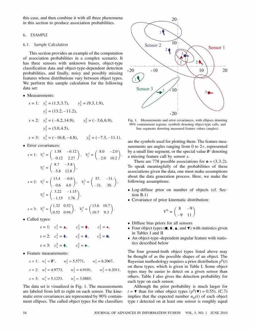
The data set is visualized in Fig. 1. The measurementsare labeled from left to right on each sensor. The kine-matic error covariances are represented by 90% contain-ment ellipses. The called object types for the classifiers

Fig. 1. Measurements and error covariances, with ellipses denoting90% containment regions, symbols denoting object-type calls, and

line segments denoting measured feature values (angles).

are the symbols used for plotting them. The feature mea-surements are angles ranging from 0 to 2¼, representedby a small line segment, or the special value 0/ s denotinga missing feature call by sensor s.

There are 778 possible associations for n= (3,3,2).To speak meaningfully of the probabilities of theseassociations given the data, one must make assumptionsabout the data generation process. Here, we make thefollowing assumptions:

² Log-diffuse prior on number of objects (cf. Sec-tion B.1)

² Covariance of prior kinematic distribution:

V0 =�

8 ¡9¡9 11

¶

² Diffuse bias priors for all sensors² Four object types (¥, ¨, N, and H) with statistics givenin Tables I and II

² An object-type—dependent angular feature with statis-tics described below

The four ground-truth object types listed above maybe thought of as the possible shapes of an object. TheBayesian methodology requires a prior distribution p0(t)on these types, which is given in Table I. Some objecttypes may be easier to detect on a given sensor thanothers. Table I also gives the detection probability foreach type on each sensor.

Although the prior probability is much larger fort=H than for other object types (p0(H) = 0:55), (C.7)implies that the expected number nD(t) of each objecttype t detected on at least one sensor is roughly equal

54 JOURNAL OF ADVANCES IN INFORMATION FUSION VOL. 5, NO. 1 JUNE 2010

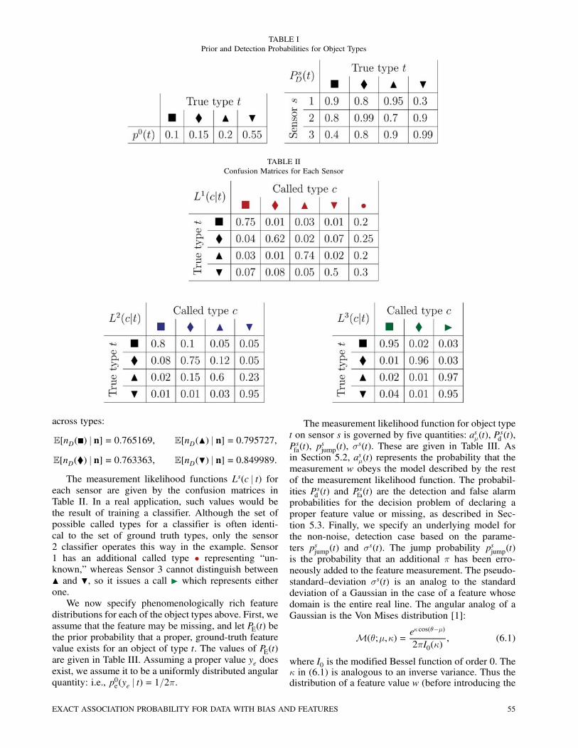
TABLE IPrior and Detection Probabilities for Object Types

TABLE IIConfusion Matrices for Each Sensor

across types:

E[nD(¥) j n] = 0:765169, E[nD(N) j n] = 0:795727,

E[nD(¨) j n] = 0:763363, E[nD(H) j n] = 0:849989:

The measurement likelihood functions Ls(c j t) foreach sensor are given by the confusion matrices inTable II. In a real application, such values would bethe result of training a classifier. Although the set ofpossible called types for a classifier is often identi-cal to the set of ground truth types, only the sensor2 classifier operates this way in the example. Sensor1 has an additional called type ² representing “un-known,” whereas Sensor 3 cannot distinguish betweenN and H, so it issues a call I which represents eitherone.

We now specify phenomenologically rich featuredistributions for each of the object types above. First, weassume that the feature may be missing, and let PE(t) bethe prior probability that a proper, ground-truth featurevalue exists for an object of type t. The values of PE(t)are given in Table III. Assuming a proper value ye doesexist, we assume it to be a uniformly distributed angularquantity: i.e., p0e(ye j t) = 1=2¼.

The measurement likelihood function for object typet on sensor s is governed by five quantities: as¹(t), P

sd (t),

Psfa(t), psjump(t), ¾

s(t). These are given in Table III. Asin Section 5.2, as¹(t) represents the probability that themeasurement w obeys the model described by the restof the measurement likelihood function. The probabil-ities Psd (t) and Psfa(t) are the detection and false alarmprobabilities for the decision problem of declaring aproper feature value or missing, as described in Sec-tion 5.3. Finally, we specify an underlying model forthe non-noise, detection case based on the parame-ters psjump(t) and ¾s(t). The jump probability psjump(t)is the probability that an additional ¼ has been erro-neously added to the feature measurement. The pseudo-standard—deviation ¾s(t) is an analog to the standarddeviation of a Gaussian in the case of a feature whosedomain is the entire real line. The angular analog of aGaussian is the Von Mises distribution [1]:

M(�;¹,·) =e·cos(�¡¹)

2¼I0(·), (6.1)

where I0 is the modified Bessel function of order 0. The· in (6.1) is analogous to an inverse variance. Thus thedistribution of a feature value w (before introducing the

EXACT ASSOCIATION PROBABILITY FOR DATA WITH BIAS AND FEATURES 55

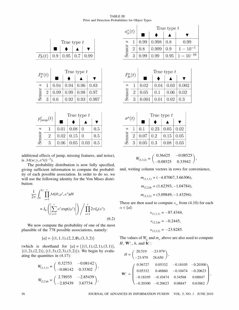
TABLE IIIPrior and Detection Probabilities for Object Types

additional effects of jump, missing features, and noise),is M(w;y,¾s(t)¡2).

The probability distribution is now fully specified,giving sufficient information to compute the probabil-ity of each possible association. In order to do so, wewill use the following identity for the Von Mises distri-bution:

12¼

Z 2¼

0

rYs=1

M(�;¹s,·s)d�

= I0

ï¯ rXs=1

·s exp(i¹s)

¯¯!,

rYs=1

2¼I0(·s):

(6.2)

We now compute the probability of one of the mostplausible of the 778 possible associations, namely:

[a] = f(1,1,1), (2,2,0/ ), (3,3,2)g(which is shorthand for [a] = ff(1,1),(2,1), (3,1)g,f(1,2),(2,2)g,f(1,3),(2,3), (3,2)g). We begin by evalu-ating the quantities in (4.17):

W(1,1,1) =�

0:32753 ¡0:08142¡0:08142 0:33302

¶,

W(2,2,0/) =�

2:78935 ¡2:85439¡2:85439 3:67734

¶,

W(3,3,2) =�

0:36425 ¡0:08525¡0:08525 0:33942

¶,

and, writing column vectors in rows for convenience,

m(1,1,1) = (¡4:87067,3:66306),

m(2,2,0/) = (1:62393,¡1:04784),

m(3,3,2) = (3:09849,¡1:43294):These are then used to compute ·® from (4.10) for each® 2 [a]:

·(1,1,1) =¡87:4344,

·(2,2,0/) =¡0:2445,

·(3,3,2) =¡23:8285:The values ofW® and m® above are also used to computeH, W¤

¡, h, and b¤¡:

H =

�20:519 ¡23:979¡23:979 28:650

¶,

W¤¡ =

0BBB@

0:56727 0:05332 ¡0:18105 ¡0:203000:05332 0:48860 ¡0:10474 ¡0:20623¡0:18105 ¡0:10474 0:34568 0:08847

¡0:20300 ¡0:20623 0:08847 0:63862

1CCCA ,

56 JOURNAL OF ADVANCES IN INFORMATION FUSION VOL. 5, NO. 1 JUNE 2010

h= (¡0:14826,1:18228),b¤¡ = (¡5:5339,¡0:04816,¡1:2648,¡6:9713):

From these we have jW¤¡j jHj= 0:473943, and b¤T¡

¢W¤¡1¡ b¤¡+ h

TH¡1h= 247:8660, so (4.20) yields ·([a])=¡248:613. Combining this in (4.8) with the values of·® we have

GK(zK , [a]) = C exp

á12

÷([a])+

X®2[a]

·®

!!

= 1:58147£ 1078C:

In addition to GK(zK , [a]) there are two other con-tributions to the association probability in (3.25). Wecompute g([a]) from (B.10). This requires the probabil-ity q that an object is undetected on all sensors, whichis given by (5.10):

q=Xt

p0(t)Ys2SQsD(t) = 0:001945 (exactly):

Therefore g([a]) = (2!=7!)0:9980555 = 0:000392981.Finally, we compute the joint object-type—feature

component GJ (zJ , [a]), which is somewhat involved.Fortunately, (3.28) and (3.29) reduce this calculationto the computation of PJ®(zJ ) for each ®, and thereare only 47 possible sets ® (compared to 778 asso-ciations). Because the feature distributions and detec-tion probabilities are object-type—dependent, for any®, PJ®(zJ ) is given by P®(c,w) in (5.15) (the J be-ing suppressed, and zJ expanded into (c,w)). This, inturn, requires the computation of P®(w j t) in (5.16) foreach object type t. We will compute P®(w j t) explic-itly for one of the sets ® in our example [a], namely®= (3,3,2) = f(1,3),(2,3), (3,2)g. To do so, we suc-cessively break down the computation in order to ac-count for various phenomena–in each case expressingP®(w j t) in terms of some simpler version of P®(w j t)which does not include the phenomenon. Specifically,we do this for noise, then missing features, then thejump by ¼.

The first phenomenon to account for is noise, sowe evaluate P®(w) using (5.22), suppressing the depen-dence on t in the notation for brevity. This requiresthat we compute P®

0¹ (w) for all eight subsets ®0 � ®,

where ®0 represents a hypothesis about which mea-surements in ® arise from the model (as opposed tonoise). To compute each P®

0¹ (w), we turn to (5.34) to

handle missing features. In this case, ®p = ®0 for any

®0 � ® because wsi is proper (i.e., non-missing) for each(s, i) 2 ®: w1

3 = 6:2067, w23 = 6:2011, and w3

2 = 3:0885.This, in turn, requires us to evaluate P®

0d (w), accounting

the the jump phenomenon. Unlike noise and missingfeatures, we do not have a general equation to accountfor the possible jump by ¼, as it is a rather specificphenomenon. Therefore we adapt (5.17) to this specificcase, providing a general formula for P®(w) (which we

then use to evaluate P®0

d (w)):

P®(w) =Zp0(y)

Y(s,i)2®

(qsjumpLs(wsi j y) +psjumpL

s(wsi ¡¼ j y))dy

=X®0�®

Y(s,i)2®0

psjump

Y(s,i)2®n®0

qsjumpP®M (w

®0 ): (6.3)

Here ®0 represents a hypothesis about which measure-ments in ® have experienced a jump by ¼, and w®

0is

the same as w, but with ¼ subtracted from each wsi forwhich (s, i) 2 ®0. Finally, we must compute the P®M (w) in(6.3). This is given by (6.2).

P®M (w) = I0

ï¯X(s,i)2®

(¾s)¡2 exp(iwsi )

¯¯!, Y

(s,i)2®2¼I0((¾

s)¡2):

(6.4)

Now, we may begin the numerical computation ofthe original P®(w j t) (including all phenomena) for®= (3,3,2) = f(1,3), (2,3),(3,2)g.

P®M (w j ¥) =I0(j0:1¡2e6:2067i+0:07¡2e6:2011i+0:05¡2e3:0885ij)

(2¼)3I0(0:1¡2)I0(0:07

¡2)I0(0:05¡2)

= 8:87511£ 10¡264:

Naturally, this value is tiny because w32 = 3:0885 is

many sigmas away from w13 and w

23. However, when we

evaluate (6.3), we sum over cases where ¼ is subtractedfrom wsi for some subset ®0 of ®. This will produce alarge value for the subset ®0 = f(3,2)g:P®M (w

®0 j ¥)

=I0(j0:1¡2e6:2067i +0:07¡2e6:2011i+0:05¡2e(3:0885¡¼)ij)

(2¼)3I0(0:1¡2)I0(0:07

¡2)I0(0:05¡2)

= 2:55152:

Naturally, the same value is produced for ®0 = f(1,3),(2,3)g, but all other ®0 � ® produce negligible values.Therefore (6.3) may be evaluated as

P®d (w j ¥) = 0:99£ 0:98£ 0:06£ 2:55152

+0:01£ 0:02£ 0:94£ 2:55152+ (tiny)

= 0:149009:

Here we use the subscript d in anticipation of the nextstep: incorporating the effects of missing features via(5.34). This will require the value of P®d (w j ¥) forone-element sets ®–this value is always equal to theprior value 1=(2¼) for this specific feature. Referringto Table III for the values of PE, P

sd and Psfa, we obtain

the following probability density which accounts for thepossibility of the object lacking the feature (and all threemeasurements in ® arising as false alarms):

P®¹ (w j ¥) = 0:9£ 0:94£ 0:99£ 0:6£ 0:149009

+0:1£ 0:02£ 0:05£0:001£ (2¼)¡3

= 0:0748806:

EXACT ASSOCIATION PROBABILITY FOR DATA WITH BIAS AND FEATURES 57

Here we use the subscript ¹ in anticipation of the finalstep: incorporating noise. For this we need values ofP®

0¹ for all subsets ®0 � ®. Repeating the above steps foreach subset yields

P(3,3,2)¹ (w j ¥) = 0:0748806, P(0/,0/,0/)

¹ (w j ¥) = 1,

P(0/,3,2)¹ (w j ¥) = 0:0289101, P(3,0/,0/)

¹ (w j ¥) = 0:134963,

P(3,0/,2)¹ (w j ¥) = 0:0193784, P(0/,3,0/)

¹ (w j ¥) = 0:142603,

P(3,3,0/)¹ (w j ¥) = 0:421703, P(0/,0/,2)

¹ (w j ¥) = 0:0859596:

Therefore

P®(w j ¥) = 0:99£ 0:8£ 0:99£ 0:0748806

+0:8£ 0:99£ 0:01£ 0:0289101£ 0:134963+ ¢ ¢ ¢+0:01£ 0:2£ 0:01£ 1£ 0:134963£ 0:142603

£ 0:0859596 = 0:0595787:

Carrying out the above computation for each objecttype t, we get

P®(w j ¥) = 0:0595787, P®(w j N) = 0:0221195,

P®(w j ¨) = 0:00999947, P®(w j H) = 2:06241:

These are the quantities needed in (5.15) to computeP®(c,w) for ®= (3,3,2). Using the parameters in Ta-bles I and II with the called types c13 = ², c23 = ¥, andc32 =I we have

P®(c,w) = 0:1£ 0:9£ 0:8£ 0:4£ 0:2£ 0:8£ 0:03

£ 0:0595787+0:15£ 0:8£ 0:99£ 0:8£ 0:25

£ 0:08£ 0:03£ 0:00999947+0:2£ 0:95£ 0:7

£ 0:9£ 0:2£ 0:02£ 0:97£ 0:0221195+0:55

£ 0:3£ 0:9£ 0:99£ 0:3£ 0:01£ 0:95£ 2:06241

= 0:000883213:

This value is the largest among three-measurementsets ®, and the eighth-largest overall. The three largestvalues are P(0/,0/,2)(c,w) = 0:00598235, P(3,0/,2)(c,w) =0:00281482, and P(3,3,0/)(c,w) = 0:00241721. After com-puting P®(c,w) for all 47 sets ®, we may use (3.29) toget RJ®(zJ ) for each ®, and then multiply them in (3.28)to get GJ (zJ , [a]). For [a] = f(1,1,1), (2,2,0/ ), (3,3,2)gthis yields

GJ (zJ , [a]) = 107662:£ 4673:65£ 548368:

= 2:75925£ 1014:

Therefore (3.25) reduces to

Pr([a] j z) = 0:000392981£ 1:58147£ 1078C

£ 2:75925£ 1014 Pr([a0] j z)= 1:71484£ 1089C0,

where C0 = C Pr([a0] j z).

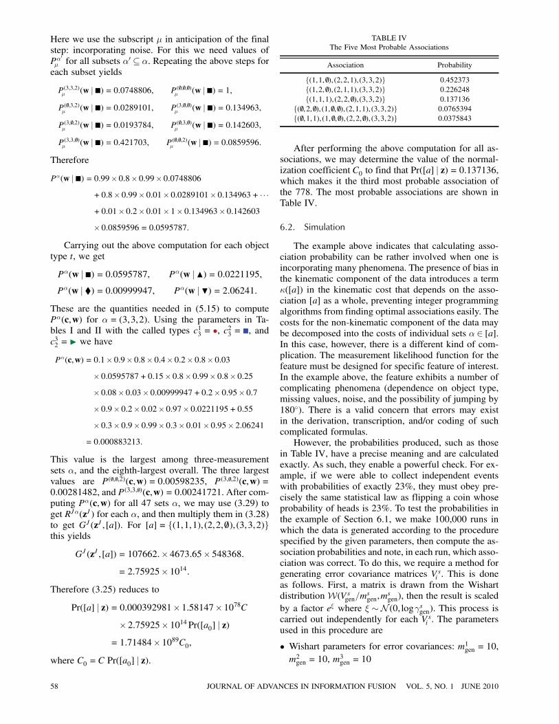
TABLE IVThe Five Most Probable Associations

Association Probability

f(1,1,0/), (2,2,1),(3,3,2)g 0.452373f(1,2,0/), (2,1,1),(3,3,2)g 0.226248f(1,1,1),(2,2,0/),(3,3,2)g 0.137136

f(0/,2,0/), (1,0/,0/), (2,1,1), (3,3,2)g 0.0765394f(0/,1,1),(1,0/,0/), (2,2,0/), (3,3,2)g 0.0375843

After performing the above computation for all as-sociations, we may determine the value of the normal-ization coefficient C0 to find that Pr([a] j z) = 0:137136,which makes it the third most probable association ofthe 778. The most probable associations are shown inTable IV.

6.2. Simulation

The example above indicates that calculating asso-ciation probability can be rather involved when one isincorporating many phenomena. The presence of bias inthe kinematic component of the data introduces a term·([a]) in the kinematic cost that depends on the asso-ciation [a] as a whole, preventing integer programmingalgorithms from finding optimal associations easily. Thecosts for the non-kinematic component of the data maybe decomposed into the costs of individual sets ® 2 [a].In this case, however, there is a different kind of com-plication. The measurement likelihood function for thefeature must be designed for specific feature of interest.In the example above, the feature exhibits a number ofcomplicating phenomena (dependence on object type,missing values, noise, and the possibility of jumping by180±). There is a valid concern that errors may existin the derivation, transcription, and/or coding of suchcomplicated formulas.

However, the probabilities produced, such as thosein Table IV, have a precise meaning and are calculatedexactly. As such, they enable a powerful check. For ex-ample, if we were able to collect independent eventswith probabilities of exactly 23%, they must obey pre-cisely the same statistical law as flipping a coin whoseprobability of heads is 23%. To test the probabilities inthe example of Section 6.1, we make 100,000 runs inwhich the data is generated according to the procedurespecified by the given parameters, then compute the as-sociation probabilities and note, in each run, which asso-ciation was correct. To do this, we require a method forgenerating error covariance matrices Vsi . This is doneas follows. First, a matrix is drawn from the Wishartdistribution W(Vsgen=m

sgen,m

sgen), then the result is scaled

by a factor e» where » »N (0, log°sgen). This process iscarried out independently for each Vsi . The parametersused in this procedure are

² Wishart parameters for error covariances: m1gen = 10,

m2gen = 10, m3

gen = 10

58 JOURNAL OF ADVANCES IN INFORMATION FUSION VOL. 5, NO. 1 JUNE 2010

² Baseline error covariances:

V1gen =

�5 1

1 7

¶,

V2gen =

�6 ¡3¡3 4

¶,

V3gen =

�7 5

5 4

¶

² Scale factors for error covariances: °1gen = 2, °2gen = 3,°3gen = 4

There are some subtleties to the simulation processdue to the diffuse nature of the priors employed, andto the requirement of not leaving extraneous signaturesin the data. There are three places where diffuse priorsoccur: in the number of objects n; in », the center of theregion of objects; and in the bias ¯s of some sensors.Appendix C shows how to simulate data efficiently witha specified number of tracks ns on each sensor, evenwhen the prior ½0 is diffuse. To circumvent directlysampling from diffuse priors for » and ¯s, we imposethe convention that scenes from sensors with diffusebias priors are pre-processed to have a centroid ofzero, and that all the other scenes are pre-processedjointly to have a centroid of zero. This renders thechoices of » and of ¯s for those sensors s with diffusepriors irrelevant because they leave no trace in thedata.

One hundred thousand runs were made for thisscenario, each run producing probabilities for each ofthe 778 possible associations. These associations weregrouped into bins: those with probability less than0.0001, those with probability between 0.0001 and0.001, etc. For example, there were 452,911 associa-tions with probability between 0.001 and 0.01. Of these,1453 were correct associations, i.e., 0.32081%. This iscertainly consistent–it lies between 0.1% and 1%–but we will demonstrate a far more stringent valida-tion.

One may consider the 77,800,000 association eventsas independent flips of biased coins with various prob-abilities pi of coming up heads (meaning “correct as-sociation”). (Technically the events are not completelyindependent but only very nearly so: two events pickedat random have a 1-in-a-100,000 chance of coming fromthe same run, and hence exhibiting dependence.) Wemay consider either the entire data set of flips, or anysubsets we like provided they are chosen without refer-ence to ground truth. The law of large numbers saysthat the number of heads in any such data set willasymptotically approach a Gaussian distribution whosemean equals the sum of pi over the events i, and whosevariance equals the sum of pi(1¡pi). Therefore, letting“tot” denote the total number of associations in a data setand “#” denote the number of these which are correct,

we have

E(#=tot) =1tot

totXi=1

pi and

¾(#=tot) =1tot

vuut totXi=1

pi(1¡pi):(6.5)

We may now make a much more incisive observa-tion about 0.32081% than the fact that it lies between0.1% and 1%. We find that E(#=tot) = 0:32728%, and¾(#=tot) = 0:00848%. Thus, not only is 0.32081% be-tween 0.1% and 1%, and not only is it close to theexpected value 0.32728%, but it is precisely 0.76 stan-dard deviations below the expected value. Furthermore,the large number of trials ensures that the distributionis approximately Gaussian, so we can convert the score³ =¡0:76 into the statement that the number of cor-rect associations lies at the 22nd percentile: i.e., it is aperfectly typical event.

Table V gives similar results for all probability bins.The first two columns specify the range of computedassociation probabilities in the bin. The third columngives the total number of associations (out of 77.8 mil-lion) with computed probabilities in the range of the bin.Column four gives the number of associations in theprobability bin which are correct (and therefore sumsto 100,000), and column five gives the fraction whichare correct (column four divided by column three). Thesixth and seventh columns give the expected value andstandard deviation of the value in column five based on(6.5). Column eight gives the number of standard devi-ations which column five is above or below its expectedvalue (i.e., ³ = (#=tot¡E(#=tot))=¾(#=tot)). Finally, col-umn nine converts column eight into the correspondingpercentile of a Gaussian distribution.

The results in Table V verify the association proba-bility formulas given in this paper in the scenario of Sec-tion 6.1. The most anomalous result is that only 99.42%of the associations with probability in the range 99% to99.9% are correct, compared to an expected value of99.53%, but this is only a 2.2 sigma event: still quitetypical. Similar results hold for events other than com-plete associations. An event of great interest, for exam-ple, is whether the association deemed most probable iscorrect. As shown in Table VI, this occurs 82.8% of thetime.

It is notable that both small and large probabili-ties are reliable–there is no failure in any probabilityrange. Similar results are presented in [10] for a simpler,but denser, scenario (two sensors, kinematic-only data).There, a comparison is made between the exact bias in-tegration formula presented in Section 4 and a method,currently considered state-of-the-art, in which the singlemost likely bias is selected and removed for each associ-ation hypothesis. Although the latter method performedreasonably accurately (17.6%, compared to 23.1% forthe exact method) the probabilities it produced were off

EXACT ASSOCIATION PROBABILITY FOR DATA WITH BIAS AND FEATURES 59

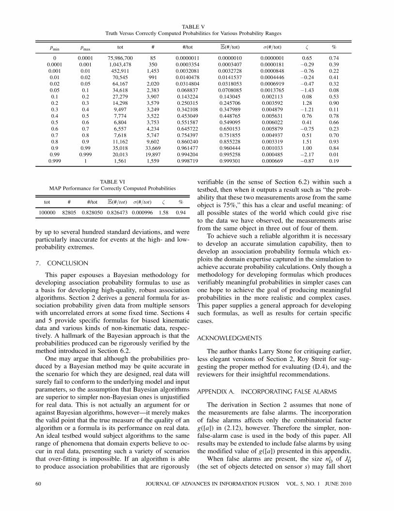
TABLE VTruth Versus Correctly Computed Probabilities for Various Probability Ranges

pmin pmax tot # #/tot E(#=tot) ¾(#=tot) ³ %

0 0.0001 75,986,700 85 0.0000011 0.0000010 0.0000001 0.65 0.740.0001 0.001 1,043,478 350 0.0003354 0.0003407 0.0000181 ¡0:29 0.390.001 0.01 452,911 1,453 0.0032081 0.0032728 0.0000848 ¡0:76 0.220.01 0.02 70,545 991 0.0140478 0.0141537 0.0004446 ¡0:24 0.410.02 0.05 64,167 2,020 0.0314804 0.0318053 0.0006919 ¡0:47 0.320.05 0.1 34,618 2,383 0.068837 0.0708085 0.0013765 ¡1:43 0.080.1 0.2 27,279 3,907 0.143224 0.143045 0.002113 0.08 0.530.2 0.3 14,298 3,579 0.250315 0.245706 0.003592 1.28 0.900.3 0.4 9,497 3,249 0.342108 0.347989 0.004879 ¡1:21 0.110.4 0.5 7,774 3,522 0.453049 0.448765 0.005631 0.76 0.780.5 0.6 6,804 3,753 0.551587 0.549095 0.006022 0.41 0.660.6 0.7 6,557 4,234 0.645722 0.650153 0.005879 ¡0:75 0.230.7 0.8 7,618 5,747 0.754397 0.751855 0.004937 0.51 0.700.8 0.9 11,162 9,602 0.860240 0.855228 0.003319 1.51 0.930.9 0.99 35,018 33,669 0.961477 0.960444 0.001033 1.00 0.840.99 0.999 20,013 19,897 0.994204 0.995258 0.000485 ¡2:17 0.010.999 1 1,561 1,559 0.998719 0.999301 0.000669 ¡0:87 0.19

TABLE VIMAP Performance for Correctly Computed Probabilities

tot # #/tot E(#=tot) ¾(#=tot) ³ %

100000 82805 0.828050 0.826473 0.000996 1.58 0.94

by up to several hundred standard deviations, and wereparticularly inaccurate for events at the high- and low-probability extremes.

7. CONCLUSION

This paper espouses a Bayesian methodology fordeveloping association probability formulas to use asa basis for developing high-quality, robust associationalgorithms. Section 2 derives a general formula for as-sociation probability given data from multiple sensorswith uncorrelated errors at some fixed time. Sections 4and 5 provide specific formulas for biased kinematicdata and various kinds of non-kinematic data, respec-tively. A hallmark of the Bayesian approach is that theprobabilities produced can be rigorously verified by themethod introduced in Section 6.2.

One may argue that although the probabilities pro-duced by a Bayesian method may be quite accurate inthe scenario for which they are designed, real data willsurely fail to conform to the underlying model and inputparameters, so the assumption that Bayesian algorithmsare superior to simpler non-Bayesian ones is unjustifiedfor real data. This is not actually an argument for oragainst Bayesian algorithms, however–it merely makesthe valid point that the true measure of the quality of analgorithm or a formula is its performance on real data.An ideal testbed would subject algorithms to the samerange of phenomena that domain experts believe to oc-cur in real data, presenting such a variety of scenariosthat over-fitting is impossible. If an algorithm is ableto produce association probabilities that are rigorously

verifiable (in the sense of Section 6.2) within such atestbed, then when it outputs a result such as “the prob-ability that these two measurements arose from the sameobject is 75%,” this has a clear and useful meaning: ofall possible states of the world which could give riseto the data we have observed, the measurements arisefrom the same object in three out of four of them.

To achieve such a reliable algorithm it is necessaryto develop an accurate simulation capability, then todevelop an association probability formula which ex-ploits the domain expertise captured in the simulation toachieve accurate probability calculations. Only though amethodology for developing formulas which producesverifiably meaningful probabilities in simpler cases canone hope to achieve the goal of producing meaningfulprobabilities in the more realistic and complex cases.This paper supplies a general approach for developingsuch formulas, as well as results for certain specificcases.

ACKNOWLEDGMENTS

The author thanks Larry Stone for critiquing earlier,less elegant versions of Section 2, Roy Streit for sug-gesting the proper method for evaluating (D.4), and thereviewers for their insightful recommendations.

APPENDIX A. INCORPORATING FALSE ALARMS

The derivation in Section 2 assumes that none ofthe measurements are false alarms. The incorporationof false alarms affects only the combinatorial factorg([a]) in (2.12), however. Therefore the simpler, non-false-alarm case is used in the body of this paper. Allresults may be extended to include false alarms by usingthe modified value of g([a]) presented in this appendix.

When false alarms are present, the size nsD of JsD(the set of objects detected on sensor s) may fall short

60 JOURNAL OF ADVANCES IN INFORMATION FUSION VOL. 5, NO. 1 JUNE 2010

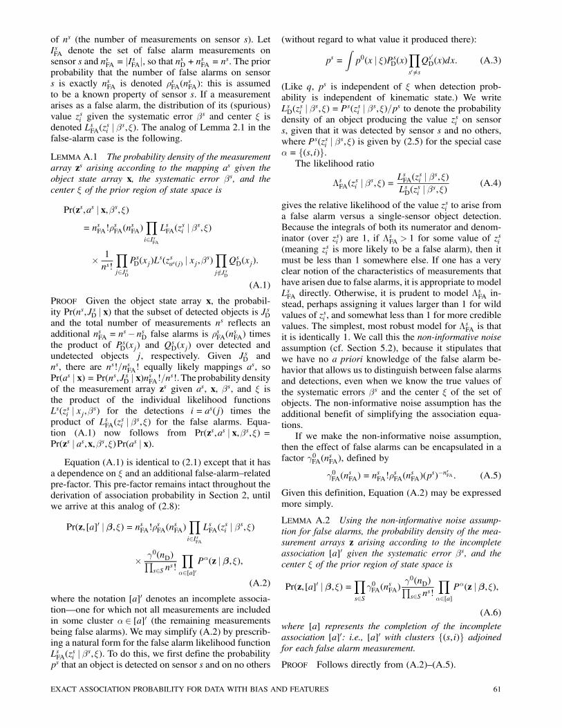
of ns (the number of measurements on sensor s). LetIsFA denote the set of false alarm measurements onsensor s and nsFA = jIsFAj, so that nsD + nsFA = ns. The priorprobability that the number of false alarms on sensors is exactly nsFA is denoted ½sFA(n

sFA): this is assumed

to be a known property of sensor s. If a measurementarises as a false alarm, the distribution of its (spurious)value zsi given the systematic error ¯s and center » isdenoted LsFA(z

si j ¯s,»). The analog of Lemma 2.1 in the

false-alarm case is the following.

LEMMA A.1 The probability density of the measurementarray zs arising according to the mapping as given theobject state array x, the systematic error ¯s, and thecenter » of the prior region of state space is

Pr(zs,as j x,¯s,»)= nsFA!½

sFA(n

sFA)

Yi2IsFA

LsFA(zsi j ¯s,»)

£ 1ns!

Yj2JsD

PsD(xj)Ls(zsas(j) j xj ,¯s)

Yj =2JsD

QsD(xj):

(A.1)

PROOF Given the object state array x, the probabil-ity Pr(ns,JsD j x) that the subset of detected objects is JsDand the total number of measurements ns reflects anadditional nsFA = ns¡ nsD false alarms is ½sFA(n

sFA) times

the product of PsD(xj) and QsD(xj) over detected andundetected objects j, respectively. Given JsD andns, there are ns!=nsFA! equally likely mappings as, soPr(as j x) = Pr(ns,JsD j x)nsFA!=ns!. Theprobability densityof the measurement array zs given as, x, ¯s, and » isthe product of the individual likelihood functionsLs(zsi j xj ,¯s) for the detections i= as(j) times theproduct of LsFA(z

si j ¯s,») for the false alarms. Equa-

tion (A.1) now follows from Pr(zs,as j x,¯s,») =Pr(zs j as,x,¯s,»)Pr(as j x).

Equation (A.1) is identical to (2.1) except that it hasa dependence on » and an additional false-alarm—relatedpre-factor. This pre-factor remains intact throughout thederivation of association probability in Section 2, untilwe arrive at this analog of (2.8):

Pr(z, [a]0 j ¯,») = nsFA!½sFA(nsFA)Yi2IsFA

LsFA(zsi j ¯s,»)

£ °0(nD)Qs2S ns!

Y®2[a]0

P®(z j ¯,»),

(A.2)

where the notation [a]0 denotes an incomplete associa-tion–one for which not all measurements are includedin some cluster ® 2 [a]0 (the remaining measurementsbeing false alarms). We may simplify (A.2) by prescrib-ing a natural form for the false alarm likelihood functionLsFA(z

si j ¯s,»). To do this, we first define the probability

ps that an object is detected on sensor s and on no others

(without regard to what value it produced there):

ps =Zp0(x j »)PsD(x)

Ys0 6=sQs

0D(x)dx: (A.3)

(Like q, ps is independent of » when detection prob-ability is independent of kinematic state.) We writeLsD(z

si j ¯s,») = Ps(zsi j ¯s,»)=ps to denote the probability

density of an object producing the value zsi on sensors, given that it was detected by sensor s and no others,where Ps(zsi j ¯s,») is given by (2.5) for the special case®= f(s, i)g.

The likelihood ratio

¤sFA(zsi j ¯s,») =

LsFA(zsi j ¯s,»)

LsD(zsi j ¯s,»)

(A.4)

gives the relative likelihood of the value zsi to arise froma false alarm versus a single-sensor object detection.Because the integrals of both its numerator and denom-inator (over zsi ) are 1, if ¤sFA > 1 for some value of zsi(meaning zsi is more likely to be a false alarm), then itmust be less than 1 somewhere else. If one has a veryclear notion of the characteristics of measurements thathave arisen due to false alarms, it is appropriate to modelLsFA directly. Otherwise, it is prudent to model ¤sFA in-stead, perhaps assigning it values larger than 1 for wildvalues of zsi , and somewhat less than 1 for more crediblevalues. The simplest, most robust model for ¤sFA is thatit is identically 1. We call this the non-informative noiseassumption (cf. Section 5.2), because it stipulates thatwe have no a priori knowledge of the false alarm be-havior that allows us to distinguish between false alarmsand detections, even when we know the true values ofthe systematic errors ¯s and the center » of the set ofobjects. The non-informative noise assumption has theadditional benefit of simplifying the association equa-tions.

If we make the non-informative noise assumption,then the effect of false alarms can be encapsulated in afactor °0FA(n

sFA), defined by

°0FA(nsFA) = n

sFA!½

sFA(n

sFA)(p

s)¡nsFA : (A.5)

Given this definition, Equation (A.2) may be expressedmore simply.

LEMMA A.2 Using the non-informative noise assump-tion for false alarms, the probability density of the mea-surement arrays z arising according to the incompleteassociation [a]0 given the systematic error ¯s, and thecenter » of the prior region of state space is

Pr(z, [a]0 j ¯,») =Ys2S°0FA(n

sFA)

°0(nD)Qs2S ns!

Y®2[a]

P®(z j ¯,»),

(A.6)

where [a] represents the completion of the incompleteassociation [a]0: i.e., [a]0 with clusters f(s, i)g adjoinedfor each false alarm measurement.

PROOF Follows directly from (A.2)—(A.5).

EXACT ASSOCIATION PROBABILITY FOR DATA WITH BIAS AND FEATURES 61

The incomplete association [a]0 distinguishes be-tween objects detected on only one sensor and falsealarms. Its completion [a] does not, but this can bequite useful in compressing the hypothesis space whenone cares only about which measurements to associate.To obtain the probability of a completion [a], we sum(A.6) over all [a]0 for which [a] is the completion. Thissum acts only on the combinatorial factors °0FA(n

sFA) and

°0(nD). To express this sum we need additional notation.Let n+D be the number of sets ® 2 [a] with at least twoelements, and ns1 be the number of measurements onsensor s which occur by themselves in [a]. We maywrite nD in terms of n+D, by noting that the number ofmeasurements on sensor s which arise from objects de-tected once only is ns1¡ nsFA, so

nD = j[a]0j= n+D +Xs2S

(ns1¡ nsFA): (A.7)

Summing (A.6) over all possible associations [a]0 yield-ing the same [a] amounts to summing over all possiblenumber of false alarms on each sensor (i.e., nsFA = 0 tons1) and accounting for all ways to choose the nsFA falsealarms from ns1 measurements. Thus we introduce thequantity

°(n+D,n1) =n11X

n1FA=0

¢ ¢ ¢nr1X

nrFA=0

°0

Ãn+D +

Xs2S

(ns1¡ nsFA)!

£Ys2S

��ns1

nsFA

¶°0FA(n

sFA)¶, (A.8)

where n1 = (n11,n21, : : : ,n

r1). The probability density

Pr(z, [a] j ¯,») may now be given by a formula identicalto (2.8), but with °0(nD) replaced by °(n+D,n1). Thus wearrive at this analog of Theorem 2.4:

THEOREM A.3 When false alarms may occur, the prob-ability of the association [a] given the measurements zis

Pr([a] j z) = g([a])G(z, [a])Pr([a0] j z), (A.9)

where

g([a]) =°(n+D,n1)°(0,n)

, (A.10)

and n denotes (n1,n2, : : : ,nr).

PROOF This follows from (A.6), and the definition(A.8).

The significance of Theorem A.3 is that the effectof false alarms is entirely encapsulated in the combina-torial factor g([a]), which is independent of the mea-surement data z. Although (A.10) is considerably morecomplicated than (2.11), it can be evaluated explicitlyand stored, if desired, for any priors ½0 and ½sFA. Moretypically, one simply assumes these priors to be Pois-son: Section B.3 gives a simple formula for g([a]) inthis case.

APPENDIX B. PRIOR ON THE NUMBER OF OBJECTS

The discussion preceding Equation (2.4) addressesthe violation of Bayesian methodology one makes whenestimating prior information from the data. This vi-olation occurs when one makes the popular assump-tion that the prior distribution of the number of objects½0(n) is Poisson with the mean number of objects esti-mated from the data. This issue is addressed here. Sec-tion B.1 computes the combinatorial factor g([a]) forseveral choices of prior ½0(n). Section B.2 demonstrateswhy the Poisson prior can work well in practice despiteits questionable validity. Finally, Section B.3 computesg([a]) explicitly for the false alarm case, assuming Pois-son priors.

B.1. The Combinatorial Factor

Poisson priorFor the Poisson prior

½0(n) = e¡ººn

n!, (B.1)

(2.9) simplifies to

°0(nD) = eº(q¡1)ºnD , (B.2)

and therefore (2.11) reduces to

g([a]) = ºnD¡nT : (B.3)

For this prior, the association probability in the absenceof systematic errors (3.2) takes the following, purelymultiplicative form

Pr([a] j z) = Pr([a0] j z)Y®2[a]+

R®(z), (B.4)

where

R®(z) =ºP®(z)Q

(s,i)2® ºPs(zsi ): (B.5)

This form is required for the traditional, efficient solu-tion of the two-sensor association problem, because itallows the cost of an association to be represented as asum of costs over each ® 2 [a]+. In the two-sensor case,one can organize these costs into a cost matrix, and findthe association with Maximal A Posteriori Probability(the MAP association) [7] using efficient integer pro-gramming techniques such as the JVC algorithm [13].The Poisson prior is the only prior on nwhich yields thispurely multiplicative form [17, 18, 19], which makes itquite convenient to use.

To use the Poisson prior, however, requires thatone estimate º from the data. For constant detectionprobabilities PsD, if one considers the probability of thenumber of tracks on each sensor given º, then one getsthe following Maximum Likelihood Estimator of º:

º =nTPs2S P

sD

: (B.6)

62 JOURNAL OF ADVANCES IN INFORMATION FUSION VOL. 5, NO. 1 JUNE 2010

This, then, is a reasonable value of º to use with thePoisson prior in practice.

A useful class of priorsFor any nonnegative integer k and any ¸ 2 [0,1), the

following prior is well defined for n 2 Z:

½0(n) = CI[n¸ k] (n¡ k)!n!

¸n, (B.7)

where the indicator function I[n¸ k] is 1 when n¸ kand 0 otherwise, and C is a normalizing constant. Forthis prior, (2.11) reduces to

g([a]) =(nD ¡ k)!(nT¡ k)!

(1¡ q)nT¡nD , (B.8)

in the limit ¸! 1¡, provided nD ¸ k. This prior has auseful interpretation in the cases k = 0 and k = 1.

Diffuse priorThe diffuse prior is obtained when k = 0. This prior

weights all possible number of objects equally, and onemight think this would be a reasonable, canonical choicefor a prior in the absence of information. In this case,(B.8) is

g([a]) =nD!nT!

(1¡ q)nT¡nD : (B.9)

This diffuse prior does not have the same claim toimpartiality as the diffuse spatial prior, however. Thespatial case has a compelling invariance with respect toEuclidean transformations which has no analog here.

Log-diffuse priorIf one had to guess an integer in the absence of any

information, the guess 5 would be better than 74,936because the latter is so specific. Rather than assuminga uniform distribution for n, we assume a uniformdistribution for logn, in accordance with Benford’s law.This yields the k = 1 case of (B.8):

g([a]) =(nD¡ 1)!(nT¡1)!

(1¡q)nT¡nD : (B.10)

This is the form of g([a]) recommended for generaluse when the computational issues favoring the Poissonprior are not important.

B.2. Justification of the Poisson prior

If we use the Poisson prior, then log(g([a]))varies linearly with nD (aside from a constant off-set): log(g([a])) = log(º)(nD ¡nT). This is the behav-ior that produces the purely multiplicative form (B.4)for Pr([a] j z). An alternative, then, to using the Poissonprior is to linearize log(g([a]) about some point n¤D fora prior one believes is appropriate.

The slope of log(g([a]) for the Poisson prior isconstant,

d

dnDlog(g([a]) = log(º), (B.11)

whereas this slope for the general prior (B.7) is

d

dnDlog(g([a]) = Ã(nD +1¡ k)¡ log(1¡ q)

¼ log�nD+1=2¡ k

1¡q¶, (B.12)

where à denotes the digamma function. Therefore thePoisson prior may, in fact, be regarded as a linearizationof the general prior (B.7) about the point

n¤D = (1¡ q)º+ k¡ 1=2: (B.13)

This is a quite reasonable place to linearize. If º is agood estimate of the number of objects (such as theMLE value º given by (B.6)), then (1¡ q)º is a goodestimate of the number of detected objects nD. Theoffset by ¡1=2 or 1=2 in the cases k = 0 or k = 1,respectively, is negligible.

Therefore, although using the Poisson prior withsome estimate of º based on the data violates Bayesianmethodology, it results in a formula that is fairly accu-rate because it is a linearization of a justifiable diffuseor log-diffuse prior on the number of objects. Becauseit is an artificially tight distribution, however, it will un-derestimate the probabilities of associations with a verylarge or a very small numbers of detected objects nD.

B.3. False Alarm Case

In contrast to ½0(n), it is quite natural to assumethe number of false alarms on a sensor is Poissondistributed. We let

½sFA(nsFA) = e

¡ºsFA (ºsFA)

nsFA

nsFA!: (B.14)

For this prior, (A.5) simplifies to

°0FA(nsFA) = e

¡ºsFA�ºsFAps

¶nsFA: (B.15)

Even with this Poisson assumption, the value ofg([a]) does not simplify much unless we also assumethat ½0(n) is Poisson distributed. If we accept (B.1) and(B.14), however, then the complicated quantity °(n+D,n1)in (A.8) simplifies to

°(n+D,n1) = exp

áº(1¡q)¡

Xs2SºsFA

!

£ ºn+DYs2S

�º+

ºsFAps

¶ns1: (B.16)

Using this, we may write (A.10) as

g([a]) = ºn+D

Ys2S

�º+

ºsFAps

¶ns1¡ns: (B.17)

EXACT ASSOCIATION PROBABILITY FOR DATA WITH BIAS AND FEATURES 63

As in the case without false alarms, the Poissonassumption results in the multiplicative form (B.4) forassociation probability, but with (B.5) replaced by

R®(z) =ºP®(z)Q

(s,i)2®

�º+

ºsFAps

¶Ps(zsi )

: (B.18)

APPENDIX C. SIMULATING A SPECIFIED NUMBEROF MEASUREMENTS

It would seem that the first step in the simulationof an association scenario would be to sample thetotal number of objects n from the prior ½0(n). In thecase of the diffuse and log-diffuse priors describedin Appendix B, this is problematic: these priors haveinfinite mean. This difficulty may be overcome by fixingn, the number of tracks observed on each sensor. Indeed,it is more convenient to gather statistics from runs witha constant value of n anyway, regardless of whether theprior ½0 forces one’s hand. One could imagine usinga rejection method to sample in this way: i.e., onecould sample n from ½0, then generate tracks on eachsensor in the usual way, but reject any scenario thatdoes not end up with n tracks on the sensors. This ishighly inefficient however. This appendix describes anefficient procedure which is statistically equivalent tothe inefficient rejection method.

We begin with the probability of an object beingdetected on some subset ® of S and not on any othersensors:

P® =Zp0(x j »)

Ys2®PsD(x)

Ys=2®QsD(x)dx: (C.1)

It is assumed that this result is independent of ». Inparticular, we are interested in two cases. First, whenPsD(x) is independent of x we have

P® =Ys2®PsDYs=2®QsD: (C.2)

On the other hand, if PsD exhibits as dependence onobject type, as in Section 5.1.1 or 5.1.2, then

P® =Xt

p0(t)Ys2®PsD(t)

Ys=2®QsD(t), (C.3)

which generalizes the formula for q given in (5.10).We define [a] to be the multiset of values of ® for

the ® 2 [a]. That is, if ®= f(1,5),(3,2)g (i.e., accordingto [a] some object produced measurement 5 on sen-sor 1, measurement 2 on sensor 3, and no others), then®= f1,3g. If there are exactly four ® 2 [a] for which®= f1,3g, then we write m(f1,3g) = 4. This multiplic-ity function m is part of the multiset [a]. After somemanipulation, we find that

Pr([a]) = °0(nD)Y®2[a]

(P®)m(®)

m(®)!: (C.4)

Each [a] determines the number of tracks n on thesensors, so we define In([a]) to be 1 if [a] is consistentwith n and 0 otherwise. The conditional probabilityPr([a] j n) is given by

Pr([a] j n) = In([a])Pr([a])P[a]0 In([a]0)Pr([a]0)

: (C.5)

This formula may be used to randomly generate [a]given n. Then, given [a], one may choose a value of[a] from the equally likely possibilities.

Having obtained a random association [a], one mustthen sample a state for each ® 2 [a], bearing in mindthe statistical influence of the fact that the object isdetected on the sensors ® and no others. In the case(C.2) of object-independent detection probabilities PsD,there is no effect on the state: it may be sampled inthe usual fashion. In the case (C.3), where PsD dependson the object type t, the object type must be sampledmore carefully, however. This requires accounting forits dependence on ®. To sample the object type t for anobject detected on sensors s 2 ® but no others, one mustdraw from Pr(t j ®) rather than p0(t), where

Pr(t j ®) = p0(t)Qs2® P

sD(t)

Qs=2® Q

sD(t)

P®

=p0(t)

Qs2® P

sD(t)

Qs=2® Q

sD(t)P

t0 p0(t0)

Qs2® P

sD(t

0)Qs=2® Q

sD(t

0):

(C.6)

When detection probability is a function of objecttype t, the distribution of object types on detectedobjects may differ greatly from p0(t). When formulatingan association scenario, it is helpful to know how manyobjects of each type to expect. The expected value ofnD(t), the number of objects of type t detected, for agiven value of n is

E[nD(t) j n] =X[a]

Pr([a] j n)X®2[a]

Pr(t j ®): (C.7)

When PsD is independent of t, Pr(t j ®) = p0(t), soE[nD(t) j n] reduces to E[nD j n]p0(t).

APPENDIX D. A CORRELATED GAUSSIAN PRODUCTFORMULA

A standard formula for the product of k Gaussiansis

kYi=1

N (x;mi,Vi) =pj2¼WjN (x;¹,W)

kYi=1

N (mi;¹,Vi),

(D.1)where

W =

ÃkXi=1

V¡1i

!¡1and ¹=W

kXi=1

V¡1i mi,

(D.2)

64 JOURNAL OF ADVANCES IN INFORMATION FUSION VOL. 5, NO. 1 JUNE 2010

and therefore

Z kYi=1

N (x;mi,Vi)dx=pj2¼Wj

kYi=1

N (mi;¹,Vi):

(D.3)

Theorem 4.2 requires the evaluation of a productof k Gaussians which is much more complicated than(D.3). Let

v =Z Z

¢ ¢ ¢Z kY

i=1

N0@ pXj=1

Aijxj ;mi,Vi

1Adx1dx2 ¢ ¢ ¢dxp,

(D.4)

where each xj 2Rn, each mi 2Rm, each Vi is a sym-metric positive definite m£m matrix, and each Aij isan m£ n matrix. In evaluating (D.4) the product over ibecomes a sum over i within the argument of the Gaus-sian, which leads to the requirement for computing thefollowing critical quantities:

Ujj 0 =kXi=1

ATijV¡1i Aij 0 for 1· j,j0 · p, (D.5)

bj =kXi=1

ATijV¡1i mi for 1· j · p and

(D.6)

c=kXi=1

mTi V¡1i mi: (D.7)

These may be used to express the integrand in (D.4) asa quadratic form over Rnp. We define

x=

0BBBB@x1

x2...

xp

1CCCCA , U=

0BBBBB@

U11 U12 ¢ ¢ ¢ U1p

U21 U22 ¢ ¢ ¢ U2p

......

. . ....

Up1 Up2 ¢ ¢ ¢ Upp

1CCCCCA and

(D.8)

b=

0BBBB@b1

b2...

bp

1CCCCA ,

so x and b are vectors in Rnp, and U is an np£ np sym-metric positive semi-definite matrix. For a broad classof matrices Aij , U is invertible and we may thereforedefine ¹=U¡1b. The integrand of (D.4) may now bewritten

kYi=1

N0@ pXj=1

Aijxj ;mi,Vi

1A= vN (x;¹,U¡1), (D.9)

provided jUj> 0, where

v =

Ãexp(c¡bTU¡1b)(2¼)mk¡npjUj

kYi=1

jVij!¡1=2

:

(D.10)

D.1 Gaussian Transformations

Theorem 4.3 requires certain formulas for manipu-lating Gaussians. First, for any invertible np£ npmatrixC, a simple algebraic manipulation shows that

N (x;¹,U¡1) = kCkN (Cx;C¹, (C¡TUC¡1)¡1),

(D.11)

where kCk denotes the absolute value of the determinantof C.

We now give a formula for integrating (D.9) overxt+1 through xp only for any 0· t· p. We let xF =(x1,x2, : : : ,xt) denote the free variables, and xI =(xt+1,xt+2, : : : ,xp) denote the variables of integration.We may then decompose U and b into correspondingblocks:

x=

�xFxI

¶, U=

�UFF UFIUIF UII

¶and b=

�bFbI

¶,

(D.12)

where UTFI =UIF . We define the following function ofxF ,

¹0I =U¡1II (bI ¡UIFxF), (D.13)

as well as the Schur complement [12] of UII in U(denoted U¤FF), and related quantities:

U¤FF =UFF ¡UFIU¡1II UIF , (D.14)

b¤F = bF ¡UFIU¡1II bI and (D.15)

¹¤F =U¤¡1FF b

¤F: (D.16)

The Gaussian in (D.9) may now be written as

N (x;¹,U¡1) =N (xF ;¹¤F ,U

¤¡1FF )N (xI;¹

0I ,U

¡1II ),

(D.17)whence Z

N (x;¹,U¡1)dxI =N (xF ;¹¤F ,U

¤¡1FF ): (D.18)

The decomposition (D.12) gives an alternative formulafor v in which the following quantities in (D.10) areexpressed in an alternative fashion:

bTU¡1b= bTI U¡1II bI +b

¤TF U

¤¡1FF b

¤F and

jUj= jUII j jU¤FF j:(D.19)

These matrix identities may also be obtained directlythrough the block matrix inversion formulas [12].

EXACT ASSOCIATION PROBABILITY FOR DATA WITH BIAS AND FEATURES 65

REFERENCES

[1] M. Abramowitz and I. A. StegunHandbook of Mathematical Functions With Formulas,Graphs, and Mathematical Tables.Dover, New York, 1964.

[2] J. Areta, Y. Bar-Shalom and M. LevedhalA hierarchical benchmark association problem in missiledefense.Signal and Data Processing of Small Targets, 2005, 382—393.

[3] Y. Bar-Shalom and H. ChenMultisensor track-to-track association for tracks with de-pendent errors.43rd IEEE Conference on Decision and Control, 2004.

[4] Y. Bar-Shalom and T. E. FortmannTracking and Data Association.Academic Press, San Diego, 1988.

[5] S. Blackman and R. PopoliDesign and Analysis of Modern Tracking Systems.Artech, Boston, 1999.

[6] C-Y. Chong and S. MoriMetrics for feature-aided track association.9th International Conference on Information Fusion, July2006.

[7] C. Y. Chong, S. Mori and K-C. ChangDistributed multitarget multisensor tracking.In Y. Bar-Shalom (Ed.), Multitarget-Multisensor Tracking:Advanced Applications, Artech, Boston, 1990.

[8] O. E. Drummond, D. A. Castanon and M. S. BellovinComparison of 2-D assignment algorithms for sparse, rect-angular, floating point, cost matrices.In Proceedings of the SDI Panels on Tracking, vol. 4, 1990.

[9] J. FerryXMAP: Track-to-track association with metric, feature, andtarget-type data.9th International Conference on Information Fusion, July2006.

[10] J. FerryExact bias removal for the track-to-track association prob-lem.12th International Conference on Information Fusion, July2009.

[11] J. P. Ferry and L. D. StoneTrack-to-track association with missing features.In Proceedings MSS Sensor and Data Fusion, May 2005.

[12] Roger A. Horn and Charles R. JohnsonMatrix analysis.Cambridge University Press, 1985.

[13] R. Jonker and A. VolgenantA shortest augmenting path algorithm for dense and sparselinear assignment problems.Computing, 38 (1987), 325—34.

[14] L. M. Kaplan and W. D. BlairAssignment costs for multiple sensor track-to-track associ-ation.7th International Conference on Information Fusion, June2004.

[15] L. M. Kaplan, W. D. Blair and Y. Bar-ShalomSimulation studies of multisensor track association andfusion methods.In Proceedings of the 2006 IEEE Aerospace Conference,Mar. 2006.

[16] S. Mori and C-Y. ChongEffects of unpaired objects and sensor biases on track-to-track association: problems and solutions.In Proceedings MSS Sensor and Data Fusion, vol. 1, 2000,137—151.

[17] S. Mori and C-Y. ChongTrack-to-track association metric–I.I.D.—Non-Poissoncases.6th International Conference on Information Fusion, July2003.

[18] S. Mori and C-Y. ChongData association hypothesis evaluation for i.i.d. but non-Poisson multiple target tracking.APIE Defense & Security 2004 Symposium on Signal andData Processing for Small Targets, 2004.

[19] S. Mori and C-Y. ChongEvaluation of data association hypotheses: Non-PoissonI.I.D. cases.7th International Conference on Information Fusion, 2004.

[20] S. Mori and C-Y. ChongHybrid multiple hypothesis data fusion for missile defensesystem object tracking and discrimination.In Proceedings MSS Sensor and Data Fusion, May 2005.

[21] K. G. MurtyAn algorithm for ranking all the assignments in order ofincreasing cost.Operations Research, 16, 3 (1968), 682—687.

[22] R. Popp, K. Pattipati and Y. Bar-Shalomm-best S-D assignment algorithm with application to mul-titarget tracking.IEEE Transactions on Aerospace and Electronic Systems, 37,1 (2001), 22—39.

[23] D. B. ReidAn algorithm for tracking multiple targets.IEEE Transactions on Automatic Control, AC-24, 6 (1979),843—854.

[24] R. A. Singer and A. J. KanyuckComputer control of multiple site correlation.Automatica, 7 (1971), 455—463.

[25] R. W. SittlerAn optimal data association problem in surveillance theory.IEEE Transactions on Military Electronics, (1964), 125—139.

[26] L. Stone, T. M. Tran and M. L. WilliamsImprovement in track-to-track association from using anadaptive threshold.12th International Conference on Information Fusion, July2009.

[27] L. D. Stone, M. L. Williams and T. M. TranTrack-to-track association and bias removal.SPIE AeroSense International Conference, Apr. 2002.

66 JOURNAL OF ADVANCES IN INFORMATION FUSION VOL. 5, NO. 1 JUNE 2010

Jim Ferry received his S.B. in mathematics from M.I.T., and his Sc.M. and Ph.D. inapplied mathematics from Brown, where he employed group representation theoryto analyze the global energetics of thermal convection.

He worked for six years at the Center for Simulation of Advanced Rockets at theUniversity of Illinois developing algorithms for simulating multiphase flows withinsolid rocket motors. Since coming to Metron in 2004, he has been the principalinvestigator of projects exploring such topics as cargo analysis, data association,network detection theory, and group tracking on dynamic networks.

EXACT ASSOCIATION PROBABILITY FOR DATA WITH BIAS AND FEATURES 67